Topics in Intelligent Control and Soft Computing

APPLICATION OF FUZZY SET THEORY IN FACILITIES LAYOUT PLANNING

Department of Civil Engineering University of Waterloo

ii

TABLE OF CONTENTS

LIST OF FIGURES ……………………………………………………….…….…. iii

LIST OF TABLES ………………………………………………………………….. v

ABSTRACT ………………………………………………………………………….. 1

INTRODUCTION ………...………………………………………………………….. 2

INTRODUCTION TO FUZZY SET THEORY …………………..………………… 3

Fuzzy Sets …………..……………………………………………….………… 3

Fuzzy Set Operations …………………………………………………………... 4

Fuzzy Linguistic Variables ………..…………………………….……………... 5

Fuzzy Control and Fuzzy Decision-Making System …………...……….……. 5

INTRODUCTION TO GENETIC ALGORITHM …………………………………… 7

LITERATURE REVIEW OF RELATED EFFORTS …………………….……..… 9

THE PROPOSED APPROACH ……………..…………………………………… 10

Generating the Weight Factors ……………………………………………… 13 Establishing the IF-THEN decision rules ………………..………………… 14

Developing a Program for the Inference of the Decision Rules to Generate the Facility Relationship Chart (FRC)……......………………… 15

Developing the Physical Layout of Facilities …….……..………….....…... 21

Evaluating the Generated Layouts ……………………………….....……… 24

COMMENTS AND DISCUSSION ……………………………………….……… 25

CONCLUSION ……………………………………………………………….……. 26

REFERENCES …………………………………………………………………… 27

iii

APPENDICES ……………………………………………………………….……. 30

Appendix A: The Weight Factors Between Each Pair of Facilities …..…. 30

Appendix B: Decision Rules …………………...………………………..….. 33

Appendix C: Visual Basic Program Listing ………………………….…… 36

Appendix D: The Max-Min Firing Rules for Facilities 2 and 4 ……..…..…... 48

Appendix E: The Overall Membership Functions ……………..……………. 63

Appendix F: Solutions Generated by Genetic Algorithms ……...………... 67

iv

LIST OF FIGURES

Fig. 1: The union of the fuzzy sets à and Õ …………………………………… 4

Fig. 2: The intersection of the fuzzy sets à and Õ ……………….……….……. 4

Fig. 3: Membership functions of the temperature linguistic variable ………… 5

Fig. 4: Basic configuration of fuzzy decision-making system .…………...…... 6 Fig. 5: Crossover in strings ………………………………………………………. 8 Fig. 6: Membership functions of material flow (MF) ………………………….. 11 Fig. 7: Membership functions of information flow (IF) ……………………..… 12 Fig. 8: Membership functions of equipment flow (EF) …………..……………… 12 Fig. 9: Membership functions of closeness rating (R) ………..………………… 12 Fig. 10: Membership functions of weight factor (WF) ……………………………. 14 Fig. 11: IF-THEN rules of (a) material flow (MF) and its weight factor (WF); (b) information flow (IF) and its weight factor; and equipment flow (EF) and its weight factor …………………………………………….. 15 Fig. 12: The part of the visual basic program used to perform the max-min rule of inference …………………………………. 16

Fig. 13: (a) Number of input variables; (b) number of membership functions for the material flow ……………………………………………. 17 Fig. 14: Values of the second membership function (low) for the material flow … 17 Fig. 15: The input value of the first variable (MF) between facilities 2 and 4…….. 18 Fig. 16: The input value of the second variable (WF) of (MF) between facilities 2 and 4 ……………………………………….. 18 Fig. 17: The total number of rules between (MF) and its (WF) …….…………… 18 Fig. 18: The membership functions of each variable in rule number 1 ……....… 19

v

Fig. 19: The fuzzy inference and defuzzification methods …………..…………… 19 Fig. 20: Overall membership functions of facilities (2-4) for material flow, information flow, and equipment flow ………………..………….… 20 Fig. 21: Facility relationship chart …………………………………………….…… 21 Fig. 22: The user interface of the genetic algorithm program ………………..…. 21 Fig. 23: Distance between facilities ……………………………………………….. 23 Fig. 24: The selected population size ……………………………………..……… 23 Fig. 25: The selected number of generations per cycle …………………..……. 24 Fig. 26: The selected layout ………………………………………………….……. 25

vi

LIST OF TABLES

Table 1. Relationships and intensity importance of factors among all facilities ……………………………………………...……… 13 Table 2. The weight factors between facilities 1 & 3 (aij) …………………...… 14 Table 3. The average closeness rating values ………………………………… 20 Table 4. Required inputs for each facility …………………………………….…. 22

1

APPLICATION OF FUZZY SET THEORY IN FACILITIES LAYOUT PLANNING

ABSTRACT

The layout of temporary facilities in a construction site deals with the selection of the most efficient layout of these facilities in order to operate efficiently and cost effectively. The layout design seeks the best arrangement of facilities within the available area. In the design process of the layout, many objectives must be considered to effectively utilize people, equipment, space, and energy. This project, therefore, proposes a methodology based on the fuzzy set theory and genetic algorithm technique to improve the layout process of facilities. The main objective of this study is to obtain the closeness rating values between each two facilities in the construction site. To achieve this objective, the fuzzy set theory and genetic algorithms technique were used to investigate the layout of temporary facilities in relation with the building(s) to be built in a construction site. An example application was presented to illustrate the proposed approach and the results were then discussed. In this example, it was assumed that the construction site consists of five temporary facilities. It is also considered that three fuzzy input factors (linguistic variables) will affect the layout process. Each of these variables will have five fuzzy sets ranging from very low to very high. Based on the above assumptions, a visual basic spreadsheet program was written for the fuzzification of the input variables, the fuzzy inference, and the defuzzification of the overall output membership functions. Initially, the fuzzification of the input variables was performed. Afterwards, the minimum operator (max-min composition rule of inference) was used and finally, the defuzzification process was applied using the centroid of the area method to convert the fuzzy output into a crisp value. The final crisp values (closeness ratings) represent the importance of the relationships between each two facilities. Using a genetic algorithm program, these values were then entered to the program along with the facilities and site areas to generate the best possible layout for these facilities in the site. Depending on the importance of relationships among the various facilities in a construction site, this study is expected to provide engineers with an appropriate tool to compare and evaluate different layouts and select the most appropriate and efficient one.

2

INTRODUCTION

The layout problem is one of the most crucial problems in the planning of service facilities, since efficient layout is critical to cost-effective operation of these facilities. Also, site space is a resource that is as important as money, time, material, labor and equipment. Despite of its importance, site planning is often neglected and the attitude of engineers has been that it will be done as the project progresses. Good facility layout, however, is important to promote safe and efficient operations, minimize travel time, decrease material handling, and avoid obstructing material and equipment movements (Tommelein et al. 1992). In the design process of the layout, therefore, many objectives must be considered to effectively utilize people, equipment, space, and energy (Tompkins and White 1984). Traditionally, in planning a layout the architect starts by making a layout diagram for the facility(ies). This diagram normally consists of different activities connected to each other. The design then proceeds by trial and error until a compromise is reached which more or less satisfies all the known factors and restrictions (Whitehead and Eldars 1965). As such, a layout is traditionally developed using relationships among the various facilities. These relationships are based on the judgement of experts that decide the importance of such relationships between each pair of facilities, which ranges from absolutely necessary to undesirable. The decision of experts, however, is vague and usually based on many quantitative or qualitative considerations for the desired closeness, or closeness relationships among the facilities. The flow of materials between facilities and the ease of supervision of employees are examples of such vague issues. Quantitative methods consider the actual transportation cost per unit time or the amount of materials moved per unit time between each two locations (Zouein 1995). Qualitative methods, on the other hand, consider a subjective numerical proximity weight to express the desirability of having any two facilities close to each other on the layout. Both methods are used in this study. In an effort to improve the layout process of facilities, this project investigates the layout of temporary facilities in a construction site in relation with the building(s) to be constructed using the fuzzy set theory (Zadeh 1965; Zadeh 1973) and genetic algorithms technique. An example application was presented to demonstrate the proposed approach and the results were then discussed. It was assumed that the construction site consists of five temporary facilities: offices, warehouse (storage), batch plant, maintenance workshop, and quality control laboratories. It is also considered that three fuzzy input factors (linguistic variables) will affect the decision of the planner of the site. These variables are: 1) material flow (MF); 2) information flow (IF); and 3) equipment flow (EF). Each of these variables will have five fuzzy sets {very low (VL), low (L), medium (M), high (H), and very high (VH)}. A visual basic spreadsheet program was developed for the fuzzification of the input variables, the fuzzy inference, and the defuzzification process. After the fuzzification of the input variables was performed, the minimum operator (Mamdani and Assilian 1975; Mamdani 1976) was used and the defuzzification

3

process was applied using the centroid of the area (COA) method to convert the fuzzy output into a crisp value. The final crisp values represent the closeness rating between each two facilities. These values were used to generate the best layout for the temporary facilities in the construction site using a genetic algorithm program. An introduction about the fuzzy set theory and genetic algorithms was first presented. The approach was explained on an application example to demonstrate its validation. The results along with the best layout obtained by the genetic algorithm technique were then presented and the advantages and drawbacks of the proposed technique were then discussed.

INTRODUCTION TO FUZZY SET THEORY The real world is complex; complexity in the world generally arises from uncertainty in the form of ambiguity. Problems featuring complexity and ambiguity have been addressed subconsciously by humans since they could think; these ubiquitous features pervade most social, technical, and economic problems faced by the human race. The fuzzy set theory was, therefore, introduced by Zadeh (1965) to deal with vague, imprecise, and uncertain problems. Fuzzy set theory has been used as a modelling tool for complex systems that are hard to define precisely, but can be controlled and operated by humans. Humans can make decisions in the absence of clearly defined boundaries based on expertise and general knowledge of the task of the system in consideration. The humans’ actions are based on the IF-THEN rules they develop over years of knowledge and experience. Fuzzy Sets A fuzzy set is a set containing elements that have varying degrees of membership in the set. Unlike the classical, or crisp, sets because members of crisp set would not be members unless their membership was full in that set (i.e., their membership is assigned a value of 1). Elements of a fuzzy set are mapped to a universe of membership value using a function-theoretic form. This function maps elements of a fuzzy set, will be denoted by Ã, to a real numbered value on the interval 0 to 1. A notation of convention for fuzzy sets when the universe of discourse X, is discrete and finite is:

When the universe, X, is continuous and infinite:

++

= L2

2~

1

1~ )()(~xx

xx

A AA µµ

= ∫ )()(~

1

1~

xx

A Aµ

4

)(),( ~~ uu OA µµ

)()()( ~~~ uuu OAN µµµ ∨=

)()()( ~~~ uuu OAN µµµ ∧=

In both notations, the horizontal bar is not a quotient but rather a delimiter. The numerator is the membership value in set à associated with the element of the universe indicated in the denominator. The + signs in the first notation is not the algebric ”add” but are a function-theoretic union. The integral sign in the second notation is not an algebric integral but a continuous function-theoretic union for continuous variables. Fuzzy Set Operations There are three basic operations that can be applied to fuzzy sets: union, intersection, and complement. Assume Ã, Õ, and Ñ are fuzzy sets in U with the membership functions and , respectively, and Ñ equals the union of à and Õ, then: Ñ= à ∪ Õ and ∀u∈U, where ∨ is the maximum as illustrated in Fig. 1 below.

Fig. 1: The union of the fuzzy sets à and Õ (Ñ= à ∪ Õ). Assuming Ñ equals the intersection of à and Õ, then: Ñ= à ∩ Õ and ∀u∈U, where ∧ is the minimum as shown in Fig. 2.

Fig. 2: The intersection of the fuzzy sets à and Õ (Ñ= à ∩ Õ).

)(~ uNµ

à Õ

u

µ

à Õ

u

µ

5

For example, if U={1,2,3,4,5,6,7}, Ã={0.8/3+1/5+0.6/6}, and Õ={0.7/3+1/4+0.5/6}, then Ñ= Ã ∪ Õ={0.8/3+1/4+1/5+0.6/6}, and Ñ= Ã ∩ Õ={0.7/3+0.5/6}. Other fuzzy set operations and properties are explained in Lin and Lee (1996). Fuzzy Linguistic Variables Linguistic variables take on values that are words in natural language, while numerical variables use numbers as values. Since words are usually less precise than numbers, linguistic variables provide a method to characterize complex systems that are ill-defined to be described in traditional quantitative terms (Zadeh1975). A linguistic variable is defined by the name of the variable x and the set term T(x) of the linguistic values of x with each value being a fuzzy number defined on U. For example, if temperature is a linguistic variable, then its term set T(temperature)={high, medium, low, . . . .}, where each term is characterized by a fuzzy set in a universe of discourse U=[0,100], as shown in Fig. 3 (Dweiri and Meier 1996). The figure shows that 70oC belongs to the linguistic variables {high, medium, and low} with membership values of {0.33,0.67,0}, respectively. Using the maximum value to find the fuzzy set (label) that this temperature value belongs to, 70oC belongs to the fuzzy set medium with a membership value of 0.67.

Fig. 3: Membership functions of the temperature linguistic variable. Fuzzy Control and Fuzzy Decision-Making System Fuzzy set theory is very useful in modelling complex and vague systems. It depicts the control actions of the operators when they can only describe their actions using natural language. Fuzzy set theory is a tool that transforms this linguistic control strategy into a mathematical control method. Fuzzy control was first used

50 65 80 70

1

0.67

0.33

Low HighMedium

Temp. oC

µ

6

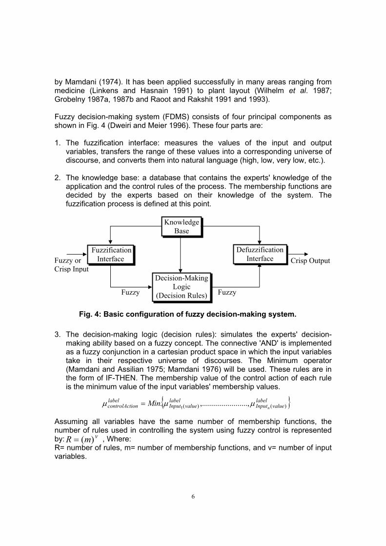
by Mamdani (1974). It has been applied successfully in many areas ranging from medicine (Linkens and Hasnain 1991) to plant layout (Wilhelm et al. 1987; Grobelny 1987a, 1987b and Raoot and Rakshit 1991 and 1993). Fuzzy decision-making system (FDMS) consists of four principal components as shown in Fig. 4 (Dweiri and Meier 1996). These four parts are: 1. The fuzzification interface: measures the values of the input and output

variables, transfers the range of these values into a corresponding universe of discourse, and converts them into natural language (high, low, very low, etc.).

2. The knowledge base: a database that contains the experts' knowledge of the

application and the control rules of the process. The membership functions are decided by the experts based on their knowledge of the system. The fuzzification process is defined at this point.

3. The decision-making logic (decision rules): simulates the experts' decision-

making ability based on a fuzzy concept. The connective 'AND' is implemented as a fuzzy conjunction in a cartesian product space in which the input variables take in their respective universe of discourses. The Minimum operator (Mamdani and Assilian 1975; Mamdani 1976) will be used. These rules are in the form of IF-THEN. The membership value of the control action of each rule is the minimum value of the input variables' membership values.

Assuming all variables have the same number of membership functions, the number of rules used in controlling the system using fuzzy control is represented by: , Where: R= number of rules, m= number of membership functions, and v= number of input variables.

{ }labelvalueInput

labelvalueInput

labelioncontrolAct n

Min )()( ....,..........,.......... µµµ1

=

vmR )(=

Knowledge Base

Decision-Making Logic

(Decision Rules)

Defuzzification Interface

Fuzzification Interface Fuzzy or

Crisp Input Crisp Output

Fuzzy Fuzzy

Fig. 4: Basic configuration of fuzzy decision-making system.

7

INTRODUCTION TO GENETIC ALGORITHMS

Genetic algorithms use the concept of Darwin's theory of evolution to search for solutions for problems in a more "natural" way. Darwin's theory stressed the fact that the existence of all living things is based on the rule of "survival of the fittest." Darwin also postulated that new breeds or classes of living things come into existence through the processes of reproduction, crossover, and mutation among existing organisms (Forrest,1993). First, different possible solutions to a problem are created. These solutions are then tested for their performance (i.e., how good a solution they provide). Among all possible solutions, a fraction of the good solutions is selected, and the others are eliminated (survival of the fittest). The selected solutions undergo the processes of reproduction, crossover, and mutation to create a new generation of possible solutions (which are expected to perform better than the previous generation). This process of production of a new generation and its evaluation is repeated until there is convergence within a generation. The benefit of this technique is that it searches for a solution from a broad spectrum of possible solutions, rather than restrict the search to a narrow domain where results would be normally expected. Genetic algorithms try to perform an intelligent search for a solution from a nearly infinite number of possible solutions (Ross 1996). All genetic algorithms contain three basic operators: reproduction, crossover, and mutation, where all three analogous to their namesakes. Let us consider the overall process of a genetic algorithm before trying to understand the basic processes. First, an initial population of n strings (for n parameters) of length L (the number of bits in each string) is created. The strings are created in a random fashion, i.e., the values of the parameters that are coded in the strings are random values (created by randomly placing the 0s and 1s in the strings). Each of the strings is decoded into a set of parameters that it represents. This set of parameters is passed through a numerical model (fitness function) of the problem space. The numerical model gives out a solution based on the input set of parameters. Based on the quality of this solution, the string is assigned a fitness value. The fitness values are determined for each string in the entire population of strings. With these fitness values, the three genetic operators are used to create a new generation of strings, which is expected to perform better than the previous generations (better fitness values). The new set of strings is again decoded and evaluated, and a new generation is created using the three basic operators. This process is continued until convergence is achieved within a population. Among the three genetic operators, reproduction is the process by which strings with better fitness values receive correspondingly better copies in the new generation, i.e. we try to ensure that better solutions persist and contribute to better offsprings (new strings) during successive generations. This is a way of

8

ensuring the "survival of the fittest" strings. Because the total number of strings in each generation is kept a constant (for computational economy and efficiency), strings with lower fitness values are eliminated. The second operator, crossover, is the process in which the strings are able to mix and match their desirable qualities in a random fashion. After reproduction, crossover proceeds in three simple steps. First, two new strings are selected at random (Fig. 5(a)). Second, a random location in both strings is selected (Fig. 5(b)). Third, the portions of the strings to the right of the randomly selected location in the two strings are exchanged (Fig. 5(c)). In this way information is exchanged and combined. Reproduction and crossover together give genetic algorithms most of their searching power. 1 0 1 1 0 0 1 0 1 1 1 0 1 1 0 0 1 0 0 1 1 0 1 1 0 0 1 1 0 1

0 1 0 0 1 1 0 1 0 1 0 1 0 0 1 1 0 1 0 1 0 1 0 0 1 1 0 0 0 1 (a) (b) (c) The third genetic operator, mutation, helps to increase the searching power. In order to understand the need for mutation, let us consider the case where reproduction of crossover may not be able to find an optimum solution to a problem. During the creation of a generation it is possible that the entire population of strings is missing a vital bit o information (e.g., none of the strings has a 1 at the fourth location) that is important for determining the correct or the most nearly optimum solution. Future generations that would be created using reproduction and crossover would be able to alleviate this problem. Here mutation becomes important. Occasionally, the value at a certain string location is changed, i.e., if there is a 1 originally at a location in the bit string, it is changed to a 0, or vice versa. Mutation thus ensures that the vital bit of information is introduced into generation. Mutation, as it does in nature, takes place very rarely, on the order of once in a thousand bit string locations (a suggested mutation rate is 0.005/bit/generation (Forrest, 1993).

Fig. 5: Crossover in strings. (a) two strings are selected at random to be mated; (b) a random location in the strings is located (here the location is before the last three bit locations); and (c) the string portions following the selected location are exchanged.

9

LITERATURE REVIEW OF RELATED EFFORTS

Various efforts have been described in the literature to deal with the site layout problem. To describe these efforts, it is important to look at several dimensions such as the tightly versus loosely packed arrangement of facilities within the site and the optimization versus heuristic approach used to solve the problem. The effort done by Cheng (1992), for example, proposes a loosely-packed solution to the layout problem using a knowledge-based system. Loosely-packed arrangement of facilities, as opposed to tightly-packed, refers to the situation when spaces are permitted between facilities. Loosely-packed arrangement, therefore, is most suitable for construction sites. Also, heuristic, as opposed to optimum solutions, refers to near-optimum solutions that are based on experience and simplified approaches. Due to the complexity of the problem, mathematical optimization was only successful for a single or very limited number of facilities (Rodriguez-Ramos and Francis 1983; Tommelein et al. 1992). This has contributed to the development of various efforts that use non-traditional techniques based on Artificial Intelligence and also to the wide use of heuristic approaches. The use of Artificial Neural Networks, for example, was proposed by Yeh (1995) to optimize a pre-determined site layout. The model minimizes a total cost function that includes the cost of constructing a facility at the assigned location on site and the cost of interacting with other facilities. The majority of researchers, however, have used heuristic approaches and knowledge-based systems to layout the facilities on a construction site in a loosely-packed manner. CONSITE (Hamiani 1987), for example, arranges facilities according to their importance and identifies their possible positions on the site. Then, it applies rule-based constraints to find the final position of each facility. Another model, SIGHTPLAN (Tommelein 1989; Tommelein et al. 1991, 1992) places temporary facilities on a construction site, one at a time, through a constraint satisfaction search. Dealing with the layout problem from different perspectives, many other researchers are also presented in the literature. The automated layout design program (ALDEP), for example, starts by selecting the first facility at random and places it starting from a given point that represents the top-left corner of the site (Seehof and Evans 1967). The next facility to be placed is the one that has the highest closeness relationship with the first facility. After placing all facilities one after the other, ALDEP uses an objective function to assign a score to the layout and then repeats the process to construct a different layout until user satisfaction. Another model, CORELAP (computerized relationship layout planning), selects the first facility to be the one with highest closeness relationship to all others (Lee and Moore 1967). Next facility to be placed is the one with highest relationship with first selected facility. In case of a tie, the facility with higher relationship to all others is selected and the procedure continues until the layout is completed. A third model, CRAFT (computer relative allocation of facilities techniques) begins with a user

10

provided layout and uses a more detailed method of calculating the desired closeness relationship between facilities by considering distances, travel cost, and material flow between facilities (Armour et al. 1964; Francis and White 1974). It then make a pair-wise location interchange of facilities which are either adjacent or have equal areas, until the layout cost can not be reduced further. In addition to the three basic models, various researchers have developed other models based primarily on these formulations such as (Rodriguez-Ramos 1982, Malakooti 1987, and Yeh 1995). Most of these efforts, however, use some simplified assumptions and do not consider the vagueness and natural language that humans use to control complex systems such as facilities planning. On the other hand, they use only a rectangular site shape and rectangular facilities with a specific aspect ratio. A facility, as such, is dealt with mainly as one block and not as a group of unit areas that can take different shapes, as being dealt with in tightly-packed arrangements. This greatly limits the possible locations in which the facility could be placed within the site. Also, heuristic and knowledge-based approaches are not guaranteed to provide optimum solutions and usually do not include an objective function to evaluate alternative layout solutions. In an attempt to overcome these limitations, this project presents a powerful methodology, based on the fuzzy set theory, to improve the facilities layout process using genetic algorithms layout optimization mechanism. Details of the proposed methodology are described and an example application is then used to validate the approach.

THE PROPOSED APPROACH

The layout problem is complex and vague. It seeks the best arrangement based on the desired closeness relationships among the facilities. These relationships are generated by the designers based on a number of factors. The larger the number of facilities in a site and the number of factors affecting the design, the more complex the layout problem becomes. The approach proposed in this study consists of the following main steps: 1) Generating the weight factors (WF) for all variables between each pair of

facilities. This is achieved using all possible factors that are believed to affect the layout.

2) Establishing the IF-THEN decision rules. 3) Developing a program for the inference of the decision rules established in the

previous step to generate the facility relationship chart (FRC). This program was used to perform the fuzzification, fuzzy inference, and defuzzification. The final crisp values obtained by the defuzzification process were then used to generate the facility relationship chart.

4) Developing the physical layout of the facilities in the construction site using the

11

generated facility relationship chart and a genetic algorithm program. 5) Evaluating the different layouts generated by the genetic algorithm program

using the judgement of the human expert. These steps were applied to an example application. In this example, it was considered that the construction site consists of five temporary facilities in addition to the building(s) to be constructed. These facilities are: 1) Offices, with an area of 160 square meters. 2) Warehouse (storage), with an area of 240 square meters. 3) Batch plant, with an area of 500 square meters. 4) Maintenance workshop, with an area of 120 square meters. 5) Quality control laboratories, with an area of 60 square meters. 6) The buildings to be constructed, which consists of two attached buildings with a

total area of 2880 square meters. As shown in Table 1, the construction site has n*(n-1)/2=6*(6-1)/2=15 relationships among all facilities, where n is the number of facilities in the site. Let us now assume that there are three factors (input variables) affecting the decision of the planner. These factors are: 1) Material flow (MF): defined by the number of parts flowing between each two

facilities in the construction site. This variable is assumed to have five membership functions as shown in Fig. 6.

2) Information flow (IF): defined by the number of communications (oral or reports) between facilities. It is also assumed that this variable has five membership functions as shown in Fig. 7.

3) Equipment flow (EF): defined by the number of material handling equipment (trucks, mixers, etc.) used to transfer materials between facilities. This variable is also assumed to have five membership functions as shown in Fig. 8.

00.20.40.60.8

11.2

0 200 400 600 800 1000 1200 1400 1600

Units /day

MF

(x)

VL VH H M L

Fig. 6: Membership functions of material flow (MF).

X

12

Based on the input variables mentioned earlier, the planner assigns a closeness rating (R) to each decision rule as an output variable. As shown in Fig. 9, the closeness rating (R) is assumed to take six membership functions (X for undesirable, U for unimportant, O for ordinary, I for important, E for especially important, and A for absolutely important).

00.20.40.60.8

11.2

0 1 2 3 4 5 6 7 8

Rating (R)

X E I O U A)( Rµ

Fig. 9: Membership functions of closeness rating (R).

X

00.20.40.60.8

11.2

0 2 4 6 8 10 12 14 16

Num be r of e quipm e nt

EF (

x)

VL VH H M L

Fig. 8: Membership functions of equipment flow (EF).

X

00.20.40.60.8

11.2

0 5 10 15 20 25 30 35 40

Num be r of com m unications /day

IF (

x)

VL VH H M L

Fig. 7: Membership functions of information flow (IF).

X

13

Generating the Weight Factors Assuming the planner was able to collect the information tabulated in Table 1 for the relationships of all factors in the layout, the weight of each factor is calculated as suggested by Saaty (1980). The numbers shown for the intensity importance Table 1. Relationships and intensity importance of factors among all facilities.

Factor 1 Factor 2 Factor 3 Intensity Importance of Factors Facilities MF IF EF 1 over 2 1 over 3 2 over 3

1-2 0 12 0 0.5 1 2 1-3 0 15 0 0.5 1 3 1-4 0 4 1 1 1 1 1-5 0 23 0 0.25 1 4 1-6 0 30 0 0.112 1 9 2-3 1200 13 10 1.5 1 1 2-4 150 3 2 1 1 1 2-5 100 5 1 2 3 2 2-6 1500 7 4 4 1 0.25 3-4 0 3 3 0.8 0.25 0.33 3-5 400 26 2 0.8 3 3 3-6 1000 5 5 4 1 0.25 4-5 0 2 1 1 1 1 4-6 0 0 2 1 1 1 5-6 5 0 1 1.25 1 0.8

of factors (aij), range from 1 for equal importance of factor i over factor j to 9 for absolute importance of factor i over factor j, where aji=1/aij (Saaty 1980). These numbers represent the true preference of each factor with respect to other factors. If the relationship between facilities 1 (offices) and 2 (warehouse) is under consideration, for example, the planner is assigning a value of 2 for the importance of factor 2 over factor 3. This means that there is a range between an equal and a weak importance of factor 2 over factor 3. On the other hand, the value of 9 assigned for the importance of factor 2 over factor 3 (considering the relationship between facilities 1 and 6) indicates an absolute importance of factor 2 over factor 3. The information shown in Table 1, however, were based on the personal judgment of the authors' previous experience in construction projects. Considering the relationship between facility 1 (offices) and facility 3 (batch plant), for example, the intensity importance of factors listed in Table 1 are used to calculate the weights of factors (Pi) shown in Table 2 below. These weights of factors are calculated in the following steps, as described in Saaty (1980):

14

1) Multiplying the n elements in each row of the shaded matrix shown in Table 2 to get the result Xi, where n is the number of factors and equals to 3 in this study.

2) Take the nth root of (Xi) for each row. The result is (Yi). 3) Normalize by dividing each number (Yi) by the sum of all the numbers (∑Yi).

The result is the weight factors Pi. Table 2. The weight factors between facilities 1 & 3 (aij).

i/j 1 2 3 Xi (=1X2X3) Yi (=X^.333) Pi= (WF) =Yi/∑Yi 1 1 0.5 1 0.5 0.794 0.240 2 2 1 3 6 1.817 0.550 3 1 0.333 1 0.333 0.693 0.210 ∑ Yi 3.304

This process is repeated for all pairs of facilities and results are listed in appendix A. The weight factor is considered one of the input factors that will influence the layout. The higher the weight factor, the more important the factor when planning the layout. The weight factor is fuzzified as shown in Fig. 10. Establishing the IF-THEN Decision Rules At this point, the fuzzification process is complete. The next step is to establish the decision-making logic (decision rules). These rules usually take the form of the IF-THEN rules. The number of decision rules between each factor and its weight factor is calculated using the equation: = (5)2 =25 , where R= number of rules, m= number of membership functions, and v= number of input variables. Since we are considering three input variables that will affect the decision of the planner, the total number of rules between each two facilities is equal to 3X25=75 rules. These rules were compiled based on the personal judgment of the authors' previous

00.20.40.60.8

11.2

0 0.2 0.4 0.6 0.8 1 1.2

We ight Factor (WF)

WF(

x)

VL VH H M L

Fig. 10: Membership functions of weight factor (WF).

vmR )(=

15

experience in construction projects. The rules are shown in Fig. 11 and listed in appendix B. MF/WF VL L M H VH IF/WF VL L M H VH EF/WF VL L M H VH

VL U U O O I VL U U U O O VL U U O I I L U O O I E L U U O O I L U O I I E M O O I E E M U O O I E M O I I E E H O I E E A H O O I E A H I I E E A

VH I E E A A VH O I E A A VH I E E A A

(a) (b) (c) U= unimportant, O= ordinary, I= important, E= especially important, A= absolutely important, VL= very low, L= low, M= medium, H= high, and VH= very high. Fig. 11: IF-THEN rules of (a) material flow (MF) and its weight factor (WF); (b)

information flow (IF) and its weight factor; and equipment flow (EF) and its weight factor.

Developing a Program for the Inference of the Decision Rules to Generate the Facility Relationship Chart (FRC) A program using Visual Basic programming language was developed to deal with the inference of the generated IF-THEN decision rules. The program can use both the max-min and max-product composition rules of inference. It also allows the user to chose any of the defuzzification methods such as the centroid of the area (COA), mean of maximum (MOM), smallest of maximum (SOM), or the largest of maximum (LOM). In this study, the max-min composition rule of inference and the centroid of the area (COA) were used for the defuzzification process required to generate the final output crisp values of the facility relationship chart. These values can then be used in the next step to develop the most efficient layout. This fuzzy decision-making process is repeated for each pair of facilities (i.e., 15 times). Parts of the program showing the use of the max-min composition rule of inference and the centroid of the area (COA) method are illustrated in Fig. 12 and Fig. 13, respectively. The complete program is listed in appendix C.

16

If DialogSheets("Dialog3").OptionButtons("MaxMin Option").Value = xlOn Then infrule= "MaxMin" Else infrule = ActiveCell.Value End If Worksheets("data1").Activate: Range("Mf1").Select: ActiveCell.Offset(0, 11).Select For j = 1 To nrul If yfire(j) = 0 Then GoTo newrule If infrule = "MaxMin" Then If mftype(l, r(j)) = "trian" Then x1fir(j) = (x2(l, r(j)) - x1(l, r(j))) * yfire(j) / y2(l, r(j)) + x1(l, r(j)) x2fir(j) = x3(l, r(j)) - (x3(l, r(j)) - x2(l, r(j))) * yfire(j) / y2(l, r(j)) Else x1fir(j) = (x2(l, r(j)) - x1(l, r(j))) * yfire(j) / y2(l, r(j)) + x1(l, r(j)) x2fir(j) = x4(l, r(j)) - (x4(l, r(j)) - x3(l, r(j))) * yfire(j) / y3(l, r(j)) End If Else If mftype(l, r(j)) = "trian" Then x1fir(j) = x2(l, r(j)): x2fir(j) = x2(l, r(j)) Else x1fir(j) = x2(l, r(j)): x2fir(j) = x3(l, r(j)) End If End If newrule: ActiveCell.Value = x1fir(j): ActiveCell.Offset(0, 1).Select: ActiveCell.Value = x2fir(j) ActiveCell.Offset(1, -1).Select Next j

Fig. 12: The part of the visual basic program used to perform the max-min rule of inference. If DialogSheets("Dialog3").OptionButtons("COA Option").Value = xlOn Then TArea = 0: Tmoa = 0 For i = 1 To s1 - 1 area(i) = xinter * ((yover(i + 1) + yover(i)) / 2) moa(i) = area(i) * (xinter / 2 + xover(i)) TArea = TArea + area(i) Tmoa = Tmoa + moa(i) Next i Fout = Tmoa / TArea

Fig. 13: The part of the visual basic program used to perform the COA defuzzification method.

When running the program, the following information are required to be entered to the program as inputs: 1) Number of variables, as shown in the screen capture of Fig. 13 (a) below. The

17

figure shows the number of variables (each variable, its weight factor, and the closeness rating).

2) Number of membership functions for each variable and the values for each membership function. For example, Fig. 13 (b) below shows the number of membership functions for the first variable, which is the material flow, while Fig. 14 shows the x-values of the second membership function (low) of this variable.

(a) (b)

Fig. 13: (a) Number of input variables; (b) number of membership functions for the material flow.

Fig. 14: Values of the second membership function (low) for the material flow.

18

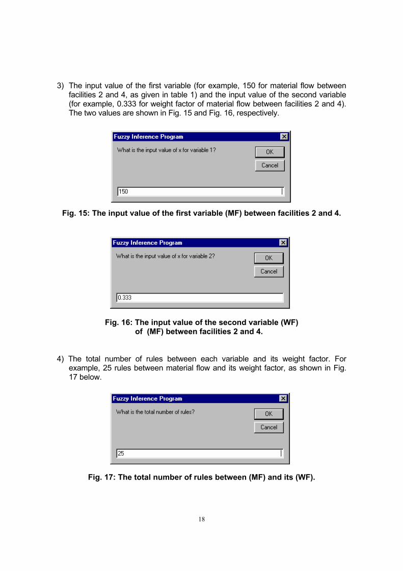
3) The input value of the first variable (for example, 150 for material flow between facilities 2 and 4, as given in table 1) and the input value of the second variable (for example, 0.333 for weight factor of material flow between facilities 2 and 4). The two values are shown in Fig. 15 and Fig. 16, respectively.

Fig. 15: The input value of the first variable (MF) between facilities 2 and 4.

Fig. 16: The input value of the second variable (WF) of (MF) between facilities 2 and 4. 4) The total number of rules between each variable and its weight factor. For

example, 25 rules between material flow and its weight factor, as shown in Fig. 17 below.

Fig. 17: The total number of rules between (MF) and its (WF).

19

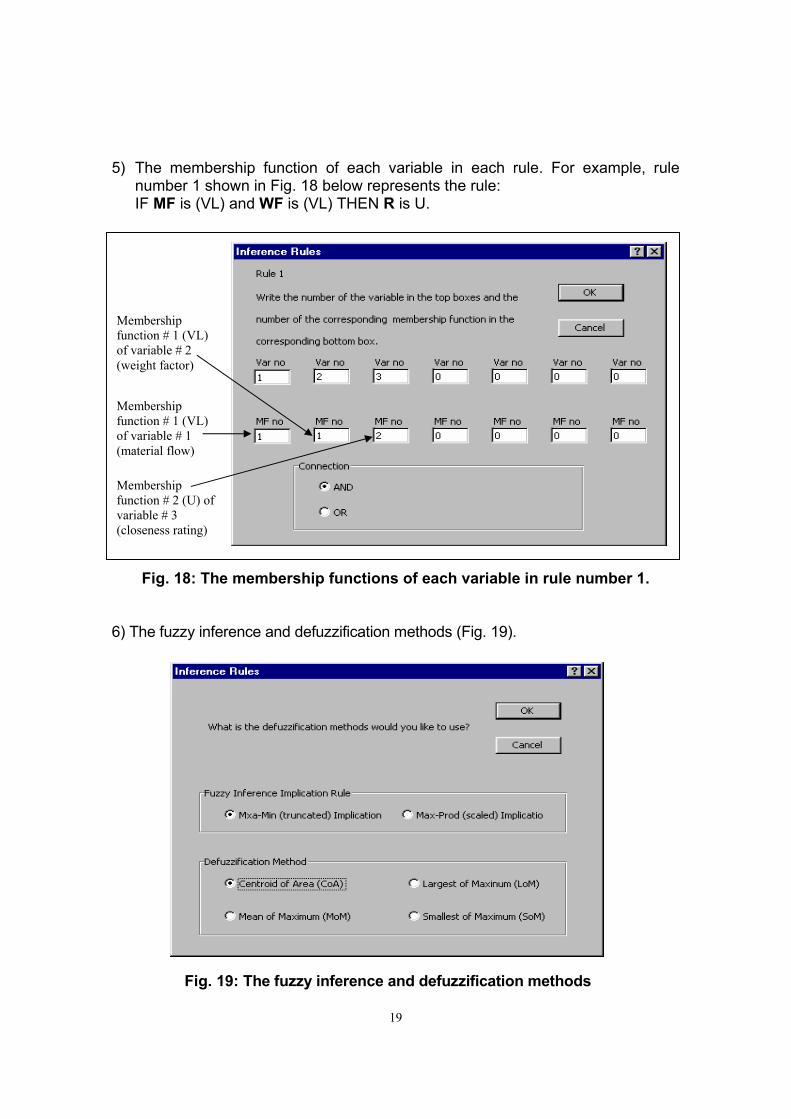
5) The membership function of each variable in each rule. For example, rule number 1 shown in Fig. 18 below represents the rule: IF MF is (VL) and WF is (VL) THEN R is U.

Fig. 18: The membership functions of each variable in rule number 1. 6) The fuzzy inference and defuzzification methods (Fig. 19).

Membership function # 1 (VL) of variable # 1 (material flow)

Membership function # 1 (VL) of variable # 2 (weight factor)

Membership function # 2 (U) of variable # 3 (closeness rating)

Fig. 19: The fuzzy inference and defuzzification methods

20

The input values for each variable shown in Table 1 were then entered to the program for each pair of facilities along with its corresponding weight factor to get the overall membership functions and their output crisp values. For example, Fig.20 illustrates the overall membership functions of facilities 2 and 4. The max-min firing rules for this pair of facilities are shown in appendix D while the overall membership functions of each pair of facilities are listed in appendix E.

Fig. 20: Overall membership functions of facilities (2-4) for material flow, information flow, and equipment flow.

The average of output crisp values (closeness ratings) for each pair of facilities is calculated in Table 3 below. These ratings are tabulated in the facility relationship chart (Fig. 21), which will be used in the next step to generate the facilities' layout in the construction site. Table 3. The average closeness rating values.

( M F/ W F)

0

0.2

0.4

0.6

0.8

1

0 2 4 6 8R at ing ( R )

( IF / W F)

0

0.2

0.4

0.6

0.8

1

0 2 4 6 8R at ing ( R )

( EF / W F)

0

0.2

0.4

0.6

0.8

1

0 2 4 6 8R at ing ( R )

Activity MF/WF IF/WF EF/WF Average1-2 2.638 4.163 2.638 3.1461-3 2.582 4.592 2.421 3.1981-4 3.001 2.759 3.501 3.0871-5 2.150 6.001 2.150 3.4341-6 2.35 6 2.35 3.5672-3 5.523 3.001 5.303 4.6092-4 3.265 2.582 4.001 3.2832-5 4.036 2.972 2.628 3.2122-6 6 2.25 5.5 4.5833-4 2.110 2.405 5.001 3.1723-5 4.100 5.667 2.928 4.2313-6 6.5 2.25 5 4.5834-5 3.001 2.421 3.501 2.9754-6 3.200 2.200 4.200 3.2005-6 3.35 2.05 4.5 3.300

21

Facility Area Facility Name (m2) # 6 5 4 3 2 1

Offices 160 1 3.567 3.434 3.087 3.198 3.146 - Warehouse 240 2 4.583 3.212 3.283 4.609 - Batch plant 500 3 4.583 4.231 3.172 -

Maintenance workshop 120 4 3.2 2.975 - Quality control labs. 60 5 3.3 -

Building to be constructed 5120 6 -

Construction site area = 98.387mx84.971m= 8360 m2.

Fig. 21: Facility relationship chart. Developing the Physical Layout of Facilities After the facility relationship chart is generated as explained in the previous step, a genetic algorithms program was used to generate the layout. The program was developed by Mr. Emad El-Beltagi, a PhD student who is currently working on the program as a part of his research work. The program requires the user to enter the number of facilities to be located in the site, the area of each facility, and the area of the construction site (Fig. 22). The figure shows that construction site is divided into 418 square units (selected as 19X22 units). Each unit has an area of 20 m2.

Fig. 22: The user interface of the genetic algorithm program.

22

As shown in Table 4 below, the user is required to enter to the program the start unit number for fixed facilities in the site (such as roads, building to be constructed, etc.). The program also requires that fixed facilities should be given the number (1), while other facilities to be given the number (0). Table 4 also summarizes the required inputs for each facility in the construction site. Due to the L shape of the building to be constructed in the site, it is divided into two parts (building 1 and building 2). This is to enable the program to place the building in its required location. Table 4. Required inputs for each facility.

Facility Status Start Unit Facility No. Facility Name Area(m2) No. of Units 1=fixed, 0=free for fixed facilities

1 Offices 160 8 0 0 2 Warehouse 240 12 0 0 3 Batch plant 500 25 0 0 4 Workshop 120 6 0 0 5 Quality control 60 3 0 0

Building 1 1440 72 1 113 6 Building 2 1440 72 1 251

The site area = 8360 m2.

To evaluate the goodness of a possible layout, an objective function was constructed by multiplying the desired closeness rating values between each two facilities by the actual distance between them, and summing up for all facilities. The objective function, as such, represents the total travel distance associated with a given site layout. Accordingly, Minimizing this objective function is required in order to arrive at the optimum layout that brings the least travel distance. Evaluating the total travel distance of a given site layout involves determining the distances between them. Considering the simplified site layout of Fig. 23, the distance dab between facilities "a" and "b" is:

95.6)105.6()93(2)(2)( 22 =−+−=−+−= bYaYbXaXabd distance

Using the distance calculations, The total travel distance (objective function) of a site layout with n facilities can be calculated as follows:

∑ ∑−

= +=

=1

1 1

n

iij

n

ijij Rdfunction)(objectivedistancetravelTotal

Where, Rij is the desired closeness rating value between facilities i and j.

23

1 2 3 4 5 6 7 8 9 10 11

1

2

3

4

5

6

7

8

9

10

11

12

Fig. 23: Distance between facilities. In the program, the user is given the flexibility to input the population size and the number of offspring generations, as shown in the screen captures of Figs. 24 and 25, respectively.

Fig. 24: The selected population size.

Distance A-dab

44

2

3

Notes: Origin O (0, 0) Point A (3, 6.5)

Point B (9,10) A

O

B

24

Fig. 25: The selected number of generations per cycle. After entering the facilities data to the program, the values for the closeness rating between each pair of facilities were taken from the results of the fuzzy inference program (Fig. 21) and was input to the program. The next step is to enter the required population size (Fig. 24) and the required number of generations per cycle (Fig. 25), which were selected as 100 and 50, respectively. After all the required inputs were entered as explained above, the genetic algorithms program generated different solutions (layouts) with their corresponding fitness values (scores), listed in appendix F. The best solution, basically, is the one with the minimum score (minimum fitness value). Evaluating the Generated Layouts The final step is to evaluate the best layouts, which is normally performed by the designer. Depending on the judgement of the designer, one layout should finally be selected which may not be the one with the best (minimum) score. Based on the personal experience of the authors, solution number 6 (shown in appendix F) was selected for the layout of the example presented in this study. This solution has a score of 622 as opposed to the solution with the minimum score (595). The selected layout is shown in Fig. 26. The shaded area in the figure represents the L-shaped building to be constructed (facility number 6). It is noticed that the offices (facility number 1) were placed near the building, which is a logical arrangement as compared to real life situations. On the other hand, the workshop (facility number 4) was placed far from the building which is also considered to be a logical placement. This is because there is no strong relation between the workshop and the building to be constructed. Also, the batch plant and the storage (facilities 2 and 3) were placed adjacent to each other. This is because of the strong relationship (closeness rating of 4.609) assigned to these two facilities.

25

4 4 4 4 4 4 3 3 3 3 3 1 1 1 1 3 3 3 3 3 6 6 6 6 6 6 1 1 1 1 2 2 2 3 3 3 3 3 6 6 6 6 6 6 2 2 2 3 3 3 3 3 6 6 6 6 6 6 2 2 2 3 3 3 3 3 6 6 6 6 6 6 2 2 2 6 6 6 6 6 6 5 5 5 6 6 6 6 6 6 6 6 6 6 6 6 6 6 6 6 6 6 6 6 6 6 6 6 6 6 6 6 6 6 6 6 6 6 6 6 6 6 6 6 6 6 6 6 6 6 6 6 6 6 6 6 6 6 6 6 6 6 6 6 6 6 6 6 6 6 6 6 6 6 6 6 6 6 6 6 6 6 6 6 6 6 6 6 6 6 6 6 6 6 6 6 6 6 6 6 6 6 6 6 6 6 6 6 6 6 6 6 6 6 6 6 6 6

Fig. 26: The selected layout.

COMMENTS AND DISCUSSION One of the drawbacks of the proposed approach is the difficulties associated with generating the membership functions of the variables affecting the decision of the planner. Another disadvantage is the problem of establishing the decision rules, which requires a great deal of care and experience. In some situations also, the planner may not efficiently decide the values for the intensity importance of factors. This is particularly true when the number of facilities increases resulting, therefore, in complex relationships between the different facilities. Often, however, site planners have adequate experience to overcome such problems. On the other hand, the main characteristics of the proposed approach that makes it an efficient system for site layout planning include: - It allows the designer (site planner) to use all possible factors affecting the

layout and utilize these factors in a scientific way instead of relying on pure

Score of current layout solution using GA (Gene No. 6) = 622 Best layout solution using GA (Gene No. 0) = 595

Start the site from here

26

judgement; - It provides different alternative solutions to the site layout and considers the

total travel distance as an objective function; - It has been implemented on a commercial spreadsheet program that is

customary to many practitioners in construction; and - This fuzzy decision-making approach can be adapted to many applications

other than the facility layout planning.

CONCLUSION In this project, a methodology was proposed based on the fuzzy set theory to generate the closeness rating values, which represent the relationships between each pair of facilities in a construction site. This was achieved using a visual basic spreadsheet program to utilize its familiar interface and powerful functions. The program performs the fuzzification of the input variables, the fuzzy inference, and the defuzzification process. The final crisp values (closeness ratings) obtained by the defuzzification process were entered into a genetic algorithms program to optimally place facilities within a construction site. An example application was presented to demonstrate the practicality and powerful capabilities of the approach and the results were then discussed. The results of the layout indicated an agreement with the real-life logical arrangement of temporary facilities in construction sites. Finally, the advantages and limitations of the proposed approach were outlined.

27

REFERENCES 1. Armour, G. C., Buffa, E. S., and Vollman, T. E. (1964). "Allocating facilities

with CRAFT." Harvard Business Review, Vol. 42, pp. 136-159. 2. Cheng, M.Y. (1992). “Automated site layout of temporary construction

facilities using geographic information systems (GIS).” Ph.D. Thesis, The University of Texas at Austin, Texas.

3. Dweiri, F. and Meier, F. A. (1996). "Application of fuzzy decision-making in

facilities layout planning." Int. J. Prod. Res., Vol. 34, No. 11, pp. 3207-3225. 4. Forrest, S. (1993). "Genetic algorithms: principles of natural selection

applied to computation." Science, Vol. 261, pp. 872-878. 5. Francis, R.L., and White, J.A. (1974). “Facility layout and location.” Prentice -

Hall, Englewood Cliffs, N.Y. 6. Grobelny, J. (1987a). "The fuzzy approach to facility layout problems."

Fuzzy Sets and Systems, Vol. 23, pp.175-190. 7. Grobelny, J. (1987b). "On one possible 'fuzzy' approach to facility layout

problems." International Journal of Production Research, Vol. 25, pp. 1123-1141.

8. Hamiani, A. (1987). “CONSITE: A knowledge-based expert system

framework for construction site layout.” Ph.D. Thesis, The University of Texas at Austin, Texas.

9. Linkens, D. A., and Hasnain, S. B. (1991). "Self-organizing fuzzy logic

control and application to muscle relaxant anaesthesia." IEE Proceedings-D, Vol. 138, pp. 274-284.

10. Lee, R. C., and Moore, J. M. (1967). "CORELAP-computerized relationship

layout planning." Journal of Industrial Engineering, Vol. 18, pp. 1994-2000. 11. Lin C-T, and Lee, C. S. (1996). "Neural fuzzy systems: a neuro-fuzzy

synergism to intelligent systems." Prentice-Hall, Inc. 12. Malakooti, B. (1987). "Computer-aided facility layout selection (CAFLAS)

with applications to multiple criteria manufacturing planning problem." Large Scale Systems, Vol. 12, No. 2, pp. 109-123.

28

13. Mamdani, E. H. (1974). "Applications of fuzzy algorithms for simple dynamic plant." IEE Proceedings, Vol. 121, pp. 1585-1588.

14. Mamdani, E. H., and Assilian, S. (1975). "An experiment in linguistic

synthesis with a fuzzy logic controller." International Journal of Man-Machine Studies, Vol. 7, pp. 1-13.

15. Mamdani, E. H. (1976). "Advances in the linguistic synthesis of fuzzy

controllers." International Journal of Man-Machine Studies, Vol. 8, pp. 669-678.

16. Raoot, A. D., and Rakshit, A. (1991). "A 'fuzzy' approach to facilities layout

planning." International Journal of Production Research, Vol. 29, pp. 835-857. 17. Raoot, A. D., and Rakshit, A. (1993). "A 'linguistic pattern' approach for

multiple criteria facilities layout problems." International Journal of Production Research, Vol. 31, pp. 203-222.

18. Rodriguez-Ramos, W.E. (1982). “Quantitative techniques for construction

site layout planning.” Ph.D. Thesis, the University of Florida. 19. Rodriguez-Ramos, W.E., and Francis, R.L. (1983). “Single crane location

optimization.” Journal of Construction Division, ASCE, Vol. 109, No. 4, pp. 387-397.

20. Ross, J. T. (1996). "Fuzzy logic with engineering applications." McGraw-

Hill, Inc, New York. 21. Saaty, T. L. (1980). "The analytical hierarchy process." McGraw-Hill, Inc,

New York. 22. Seehof, J. M., and Evans, W. O. (1967). "Automated Layout Design

Program." Journal of Industrial Engineering, Vol. 18, pp. 690-695. 23. Tommelein, I.D. (1989). “ SightPlan: an expert system that models and

augments human decision-making for designing construction site layout.” Ph.D. Thesis, Stanford University, Stanford, California.

24. Tommelein, I.D., Levitt, R.E., and Hayes-Roth, B. and Confrey, T. (1991).

“Sight plan experiments: alternative strategies for site layout design.” Journal of Computing in Civil Engineering, ASCE, Vol. 5, No. 1, pp. 42-63.

29

25. Tommelein, I.D., Levitt, R.E., and Hayes-Roth, B. (1992). “Sight layout modeling: how can artificial intelligence help?” J. Constr. Engrg. and Mngmt., ASCE, Vol. 118, No. 3, pp. 594-611.

26. Tompkins, J. A., and White, J. A. (1984). "Facilities planning." (New York:

Wiley). 27. Whitehead, B. and Eldars, M. Z. (1965). "The planning of single-storey

layouts." Building Science, Pergamon Press, Vol. 1, pp. 127-139. 28. Wivhelm, M. R., Karwowski, W., and Evans, G. W. (1987). "A fuzzy set

Approach to layout analysis." International Journal of Production Research, Vol. 25, pp. 1431-1450.

29. Yeh, I. C. (1995). "Construction site layout using annealed neutral

network." Journal of Computing in Civil engineering, ASCE, Vol. 9, No. 3, pp. 201-208.

30. Zadeh, L.A. (1965). "Fuzzy sets." Information and Control, Vol. 8, pp. 338-

353. 31. Zadeh, L.A. (1973). "Outline of a new approach to the analysis of complex

systems and decision processes." IEEE Transactions on Systems, Man and Cybernetics, SMC-3, pp. 28-44.

32. Zadeh, L. (1975). "The concept of a linguistic variable and its application

to approximate reasoning, parts 1, 2, and 3." Inf. Sci., vol. 8. 33. Zouein, P.P. (1995). “Move schedule: a planning tool for scheduling

space use on construction sites.” Ph.D. Thesis, The University of Michigan, Michigan.

30

APPENDICES

Appendix A: The Weight Factors Between Each Pair of Facilities.

1) Facilities 1 & 2: I/j 1 2 3 Xi (=1X2X3) Yi (=X^.333) Pi= (WF) =Yi/∑Yi 1 1 0.5 1 0.5 0.794 0.250 2 2 1 2 4 1.587 0.500 3 1 0.5 1 0.5 0.794 0.250 ∑ Yi 3.175

2) Facilities 1 & 3:

i/j 1 2 3 Xi (=1X2X3) Yi (=X^.333) Pi= (WF) =Yi/∑Yi 1 1 0.5 1 0.5 0.794 0.240 2 2 1 3 6 1.817 0.550 3 1 0.333 1 0.333 0.693 0.210 ∑ Yi 3.304

3) Facilities 1 & 4:

i/j 1 2 3 Xi (=1X2X3) Yi (=X^.333) Pi= (WF) =Yi/∑Yi 1 1 1 1 1 1.000 0.333 2 1 1 1 1 1.000 0.333 3 1 1 1 1 1.000 0.333 ∑ Yi 3.000

4) Facilities 1 & 5:

i/j 1 2 3 Xi (=1X2X3) Yi (=X^.333) Pi= (WF) =Yi/∑Yi 1 1 0.25 1 0.25 0.630 0.167 2 4 1 4 16 2.520 0.667 3 1 0.25 1 0.25 0.630 0.167 ∑ Yi 3.780

5) Facilities 1 & 6:

i/j 1 2 3 Xi (=1X2X3) Yi (=X^.333) Pi= (WF) =Yi/∑Yi 1 1 0.111 1 0.111 0.481 0.091 2 9 1 9 81 4.327 0.818 3 1 0.111 1 0.111 0.481 0.091 ∑ Yi 5.288

31

6) Facilities 2 & 3: i/j 1 2 3 Xi (=1X2X3) Yi (=X^.333) Pi= (WF) =Yi/∑Yi 1 1 1.5 1 1.500 1.145 0.379 2 0.667 1 1 0.667 0.874 0.289 3 1 1 1 1.000 1.000 0.331 ∑ Yi 3.018

7) Facilities 2 & 4:

i/j 1 2 3 Xi (=1X2X3) Yi (=X^.333) Pi= (WF) =Yi/∑Yi 1 1 1 1 1 1.000 0.333 2 1 1 1 1 1.000 0.333 3 1 1 1 1 1.000 0.333 ∑ Yi 3.000

8) Facilities 2 & 5:

i/j 1 2 3 Xi (=1X2X3) Yi (=X^.333) Pi= (WF) =Yi/∑Yi 1 1 2 3 6.000 1.817 0.540 2 0.5 1 2 1.000 1.000 0.297 3 0.333 0.5 1 0.167 0.550 0.163 ∑ Yi 3.367

9) Facilities 2 & 6:

i/j 1 2 3 Xi (=1X2X3) Yi (=X^.333) Pi= (WF) =Yi/∑Yi 1 1 4 1 4.000 1.587 0.444 2 0.25 1 0.25 0.063 0.397 0.111 3 1 4 1 4.000 1.587 0.444 ∑ Yi 3.572

10) Facilities 3 & 4:

i/j 1 2 3 Xi (=1X2X3) Yi (=X^.333) Pi= (WF) =Yi/∑Yi 1 1 0.8 0.25 0.200 0.585 0.162 2 1.25 1 0.333 0.416 0.747 0.206 3 4 3 1 12.000 2.289 0.632 ∑ Yi 3.621

11) Facilities 3 & 5:

i/j 1 2 3 Xi (=1X2X3) Yi (=X^.333) Pi= (WF) =Yi/∑Yi 1 1 0.8 3 2.400 1.339 0.397 2 1.25 1 3 3.750 1.554 0.461 3 0.333 0.333 1 0.111 0.480 0.142 ∑ Yi 3.373

32

12) Facilities 3 & 6: i/j 1 2 3 Xi (=1X2X3) Yi (=X^.333) Pi= (WF) =Yi/∑Yi 1 1 4 1 4.000 1.587 0.444 2 0.25 1 0.25 0.063 0.397 0.111 3 1 4 1 4.000 1.587 0.444 ∑ Yi 3.572

13) Facilities 4 & 5:

i/j 1 2 3 Xi (=1X2X3) Yi (=X^.333) Pi= (WF) =Yi/∑Yi 1 1 1 1 1 1.000 0.333 2 1 1 1 1 1.000 0.333 3 1 1 1 1 1.000 0.333 ∑ Yi 3.000

14) Facilities 4 & 6:

i/j 1 2 3 Xi (=1X2X3) Yi (=X^.333) Pi= (WF) =Yi/∑Yi 1 1 1 1 1 1.000 0.333 2 1 1 1 1 1.000 0.333 3 1 1 1 1 1.000 0.333 ∑ Yi 3.000

15) Facilities 5 & 6:

i/j 1 2 3 Xi (=1X2X3) Yi (=X^.333) Pi= (WF) =Yi/∑Yi 1 1 1.25 1 1.25 1.077 0.357 2 0.8 1 0.8 0.64 0.862 0.286 3 1 1.25 1 1.25 1.077 0.357 ∑ Yi 3.016

33

Appendix B: Decision Rules.

1) Inference rules between material flow and its weight factor: Rule 1: IF (MF) is VL AND its (WF) is VL THEN Rating (R) is U Rule 2: IF (MF) is VL AND its (WF) is L THEN Rating (R) is U Rule 3: IF (MF) is VL AND its (WF) is M THEN Rating (R) is O Rule 4: IF (MF) is VL AND its (WF) is H THEN Rating (R) is O Rule 5: IF (MF) is VL AND its (WF) is VH THEN Rating (R) is I Rule 6: IF (MF) is L AND its (WF) is VL THEN Rating (R) is U Rule 7: IF (MF) is L AND its (WF) is L THEN Rating (R) is O Rule 8: IF (MF) is L AND its (WF) is M THEN Rating (R) is O Rule 9: IF (MF) is L AND its (WF) is H THEN Rating (R) is I Rule 10: IF (MF) is L AND its (WF) is VH THEN Rating (R) is E Rule 11: IF (MF) is M AND its (WF) is VL THEN Rating (R) is O Rule 12: IF (MF) is M AND its (WF) is L THEN Rating (R) is O Rule 13: IF (MF) is M AND its (WF) is M THEN Rating (R) is I Rule 14: IF (MF) is M AND its (WF) is H THEN Rating (R) is E Rule 15: IF (MF) is M AND its (WF) is VH THEN Rating (R) is E Rule 16: IF (MF) is H AND its (WF) is VL THEN Rating (R) is O Rule 17: IF (MF) is H AND its (WF) is L THEN Rating (R) is I Rule 18: IF (MF) is H AND its (WF) is M THEN Rating (R) is E Rule 19: IF (MF) is H AND its (WF) is H THEN Rating (R) is E Rule 20: IF (MF) is H AND its (WF) is VH THEN Rating (R) is A Rule 21: IF (MF) is VH AND its (WF) is VL THEN Rating (R) is I Rule 22: IF (MF) is VH AND its (WF) is L THEN Rating (R) is E Rule 23: IF (MF) is VH AND its (WF) is M THEN Rating (R) is E Rule 24: IF (MF) is VH AND its (WF) is H THEN Rating (R) is A Rule 25: IF (MF) is VH AND its (WF) is VH THEN Rating (R) is A 2) Inference rules between information flow and its weight factor: Rule 1: IF (IF) is VL AND its (WF) is VL THEN Rating (R) is U Rule 2: IF (IF) is VL AND its (WF) is L THEN Rating (R) is U Rule 3: IF (IF) is VL AND its (WF) is M THEN Rating (R) is U Rule 4: IF (IF) is VL AND its (WF) is H THEN Rating (R) is O Rule 5: IF (IF) is VL AND its (WF) is VH THEN Rating (R) is O

34

Rule 6: IF (IF) is L AND its (WF) is VL THEN Rating (R) is U Rule 7: IF (IF) is L AND its (WF) is L THEN Rating (R) is U Rule 8: IF (IF) is L AND its (WF) is M THEN Rating (R) is O Rule 9: IF (IF) is L AND its (WF) is H THEN Rating (R) is O Rule 10: IF (IF) is L AND its (WF) is VH THEN Rating (R) is I Rule 11: IF (IF) is M AND its (WF) is VL THEN Rating (R) is U Rule 12: IF (IF) is M AND its (WF) is L THEN Rating (R) is O Rule 13: IF (IF) is M AND its (WF) is M THEN Rating (R) is O Rule 14: IF (IF) is M AND its (WF) is H THEN Rating (R) is I Rule 15: IF (IF) is M AND its (WF) is VH THEN Rating (R) is E Rule 16: IF (IF) is H AND its (WF) is VL THEN Rating (R) is O Rule 17: IF (IF) is H AND its (WF) is L THEN Rating (R) is O Rule 18: IF (IF) is H AND its (WF) is M THEN Rating (R) is I Rule 19: IF (IF) is H AND its (WF) is H THEN Rating (R) is E Rule 20: IF (IF) is H AND its (WF) is VH THEN Rating (R) is A Rule 21: IF (IF) is VH AND its (WF) is VL THEN Rating (R) is O Rule 22: IF (IF) is VH AND its (WF) is L THEN Rating (R) is I Rule 23: IF (IF) is VH AND its (WF) is M THEN Rating (R) is E Rule 24: IF (IF) is VH AND its (WF) is H THEN Rating (R) is A Rule 25: IF (IF) is VH AND its (WF) is VH THEN Rating (R) is A 3) Inference rules between equipment flow and its weight factor: Rule 1: IF (EF) is VL AND its (WF) is VL THEN Rating (R) is U Rule 2: IF (EF) is VL AND its (WF) is L THEN Rating (R) is U Rule 3: IF (EF) is VL AND its (WF) is M THEN Rating (R) is O Rule 4: IF (EF) is VL AND its (WF) is H THEN Rating (R) is I Rule 5: IF (EF) is VL AND its (WF) is VH THEN Rating (R) is I Rule 6: IF (EF) is L AND its (WF) is VL THEN Rating (R) is U Rule 7: IF (EF) is L AND its (WF) is L THEN Rating (R) is O Rule 8: IF (EF) is L AND its (WF) is M THEN Rating (R) is I Rule 9: IF (EF) is L AND its (WF) is H THEN Rating (R) is I Rule 10: IF (EF) is L AND its (WF) is VH THEN Rating (R) is E

35

Rule 11: IF (EF) is M AND its (WF) is VL THEN Rating (R) is O Rule 12: IF (EF) is M AND its (WF) is L THEN Rating (R) is I Rule 13: IF (EF) is M AND its (WF) is M THEN Rating (R) is I Rule 14: IF (EF) is M AND its (WF) is H THEN Rating (R) is E Rule 15: IF (EF) is M AND its (WF) is VH THEN Rating (R) is E Rule 16: IF (EF) is H AND its (WF) is VL THEN Rating (R) is I Rule 17: IF (EF) is H AND its (WF) is L THEN Rating (R) is I Rule 18: IF (EF) is H AND its (WF) is M THEN Rating (R) is E Rule 19: IF (EF) is H AND its (WF) is H THEN Rating (R) is E Rule 20: IF (EF) is H AND its (WF) is VH THEN Rating (R) is A Rule 21: IF (EF) is VH AND its (WF) is VL THEN Rating (R) is I Rule 22: IF (EF) is VH AND its (WF) is L THEN Rating (R) is E Rule 23: IF (EF) is VH AND its (WF) is M THEN Rating (R) is E Rule 24: IF (EF) is VH AND its (WF) is H THEN Rating (R) is A Rule 25: IF (EF) is VH AND its (WF) is VH THEN Rating (R) is A

36

Appendix C: Visual Basic Program Listing. Public inp, i, j, k As Integer Public nomf() As Integer Public fout As Double Public nrul As Integer Public nr As Integer Public xinter As Single Public TArea As Single Public mftype() As String Public connect() As String Public x1(), x2(), x3(), x4(), y1(), y2(), y3(), y4() As Single Public x() As Single Public y() As Single Public yfire() As Single Public yover() As Single Public xover() As Single Public v1(), v2(), v3(), v4(), v5(), v6(), v7() As Integer Public m1(), m2(), m3(), m4(), m5(), m6(), m7() As Integer Public z1(), z2(), z3(), z4(), z5(), z6(), z7() As Single Public x1fir(), x2fir() As Single Public Zmin(), Zmax() As Single Public slope() As Single Public Xmin(), Xmax() As Single Sub Data1() Application.ScreenUpdating = False methodofinp = Val(InputBox("Inter 1 for using interface windows, or 2 for using spredsheet", "Fuzzy Inference Program", "1")) If methodofinp = 1 Then inp = Val(InputBox("How many input variables?", "Fuzzy Inference Program", "2")) Else Worksheets("data").Select: Range("NVariables").Select: inp = ActiveCell.Value End If ReDim nomf(inp) As Integer ReDim Xmin(inp), Xmax(inp) As Single k = 0 Worksheets("data").Select: Range("NMF").Select For i = 1 To inp If methodofinp = 1 Then nomf(i) = Val(InputBox("How many membership functions per variable " & i & "?", "Fuzzy Inference Program", "1")) Else nomf(i) = ActiveCell.Value: ActiveCell.Offset(0, 1).Select End If If nomf(i) > k Then k = nomf(i) Next i ReDim mftype(inp, k) As String ReDim x1(inp, k), x2(inp, k), x3(inp, k), x4(inp, k), y1(inp, k), y2(inp, k), y3(inp, k), y4(inp, k) As Single Worksheets("data").Select: Range("MFType").Select

37

For i = 1 To inp Xmax(i) = -10000: Xmin(i) = 10000 For j = 1 To nomf(i) If methodofinp = 1 Then DialogSheets("Dialog1").Labels("Var No label").Caption = "Variable " & i DialogSheets("Dialog1").Labels("Mf No label").Caption = "Membership function " & j DialogSheets("Dialog1").Show If DialogSheets("Dialog1").OptionButtons("Trian Option").Value = xlOn Then mftype(i, j) = "trian" With DialogSheets("Dialog1") x1(i, j) = Val(.EditBoxes("First Val Edit").Caption) If x1(i, j) > Xmax(i) Then Xmax(i) = x1(i, j) If x1(i, j) < Xmin(i) Then Xmin(i) = x1(i, j) y1(i, j) = 0 x2(i, j) = Val(.EditBoxes("Second Val Edit").Caption) If x2(i, j) > Xmax(i) Then Xmax(i) = x2(i, j) If x2(i, j) < Xmin(i) Then Xmin(i) = x2(i, j) y2(i, j) = 1 x3(i, j) = Val(.EditBoxes("Third Val Edit").Caption) If x3(i, j) > Xmax(i) Then Xmax(i) = x3(i, j) If x3(i, j) < Xmin(i) Then Xmin(i) = x3(i, j) y3(i, j) = 0 End With Else mftype(i, j) = "trap" With DialogSheets("Dialog1") x1(i, j) = Val(.EditBoxes("First Val Edit").Caption) If x1(i, j) > Xmax(i) Then Xmax(i) = x1(i, j) If x1(i, j) < Xmin(i) Then Xmin(i) = x1(i, j) y1(i, j) = 0 x2(i, j) = Val(.EditBoxes("Second Val Edit").Caption) If x2(i, j) > Xmax(i) Then Xmax(i) = x2(i, j) If x2(i, j) < Xmin(i) Then Xmin(i) = x2(i, j) y2(i, j) = 1 x3(i, j) = Val(.EditBoxes("Third Val Edit").Caption) If x3(i, j) > Xmax(i) Then Xmax(i) = x3(i, j) If x3(i, j) < Xmin(i) Then Xmin(i) = x3(i, j) y3(i, j) = 1 x4(i, j) = Val(.EditBoxes("Fourth Val Edit").Caption) If x4(i, j) > Xmax(i) Then Xmax(i) = x4(i, j) If x4(i, j) < Xmin(i) Then Xmin(i) = x4(i, j) y4(i, j) = 0 End With End If Else mftype(i, j) = ActiveCell.Value If mftype(i, j) = "trian" Then ActiveCell.Offset(0, 1).Select: x1(i, j) = ActiveCell.Value If x1(i, j) > Xmax(i) Then Xmax(i) = x1(i, j): If x1(i, j) < Xmin(i) Then Xmin(i) = x1(i, j) y1(i, j) = 0: ActiveCell.Offset(0, 1).Select: x2(i, j) = ActiveCell.Value If x2(i, j) > Xmax(i) Then Xmax(i) = x2(i, j): If x2(i, j) < Xmin(i) Then Xmin(i) = x2(i, j) y2(i, j) = 1: ActiveCell.Offset(0, 1).Select: x3(i, j) = ActiveCell.Value If x3(i, j) > Xmax(i) Then Xmax(i) = x3(i, j): If x3(i, j) < Xmin(i) Then Xmin(i) = x3(i, j)

38

y3(i, j) = 0: ActiveCell.Offset(1, -3).Select Else ActiveCell.Offset(0, 1).Select: x1(i, j) = ActiveCell.Value If x1(i, j) > Xmax(i) Then Xmax(i) = x1(i, j): If x1(i, j) < Xmin(i) Then Xmin(i) = x1(i, j) y1(i, j) = 0: ActiveCell.Offset(0, 1).Select: x2(i, j) = ActiveCell.Value If x2(i, j) > Xmax(i) Then Xmax(i) = x2(i, j): If x2(i, j) < Xmin(i) Then Xmin(i) = x2(i, j) y2(i, j) = 1: ActiveCell.Offset(0, 1).Select: x3(i, j) = ActiveCell.Value If x3(i, j) > Xmax(i) Then Xmax(i) = x3(i, j): If x3(i, j) < Xmin(i) Then Xmin(i) = x3(i, j) y3(i, j) = 1: ActiveCell.Offset(0, 1).Select: x4(i, j) = ActiveCell.Value If x4(i, j) > Xmax(i) Then Xmax(i) = x4(i, j): If x4(i, j) < Xmin(i) Then Xmin(i) = x4(i, j) y4(i, j) = 0: ActiveCell.Offset(1, -4).Select End If End If Next j Next i Worksheets("data1").Select Range("Fdata").ClearContents: Range("start").Select Range("Start").Value = "No of Variables": ActiveCell.Offset(0, 1).Select: ActiveCell.Value = inp Range("variable").Select ActiveCell.Value = "Variable No": ActiveCell.Offset(0, 1).Select: ActiveCell.Value = "No. of MF" ActiveCell.Offset(0, 1).Select: ActiveCell.Value = "Xmin": ActiveCell.Offset(0, 1).Select: ActiveCell.Value = "Xmax" For i = 1 To inp Range("variable").Select: ActiveCell.Offset(i, 0).Select ActiveCell.Value = i: ActiveCell.Offset(0, 1).Select: ActiveCell.Value = nomf(i) ActiveCell.Offset(0, 1).Select: ActiveCell.Value = Xmin(i): ActiveCell.Offset(0, 1).Select: ActiveCell.Value = Xmax(i) Next i Range("Mf").Select: ActiveCell.Value = "Variable No": ActiveCell.Offset(0, 1).Select: ActiveCell.Value = "MF No" ActiveCell.Offset(0, 1).Select: ActiveCell.Value = "MF Type": ActiveCell.Offset(0, 1).Select: ActiveCell.Value = "Pint 1" ActiveCell.Offset(0, 1).Select: ActiveCell.Value = "Point 2": ActiveCell.Offset(0, 1).Select: ActiveCell.Value = "Point 3" ActiveCell.Offset(0, 1).Select: ActiveCell.Value = "Point 4": ActiveCell.Offset(0, 1).Select: ActiveCell.Value = "X" ActiveCell.Offset(0, 1).Select: ActiveCell.Value = "Y": ActiveCell.Offset(0, 1).Select: ActiveCell.Value = "Rule no" ActiveCell.Offset(0, 1).Select: ActiveCell.Value = "Yfir": ActiveCell.Offset(0, 1).Select: ActiveCell.Value = "X1fir" ActiveCell.Offset(0, 1).Select: ActiveCell.Value = "X2fir" Range("Mf1").Select For i = 0 To inp - 1 ActiveCell.Value = i + 1: ActiveCell.Offset(0, 1).Select For j = 1 To nomf(i + 1) ActiveCell.Value = j: ActiveCell.Offset(0, 1).Select ActiveCell.Value = mftype(i + 1, j): ActiveCell.Offset(0, 1).Select: ActiveCell.Value = x1(i + 1, j) ActiveCell.Offset(0, 1).Select: ActiveCell.Value = x2(i + 1, j): ActiveCell.Offset(0, 1).Select:

39

ActiveCell.Value = x3(i + 1, j) ActiveCell.Offset(0, 1).Select: ActiveCell.Value = x4(i + 1, j): ActiveCell.Offset(1, -3).Select ActiveCell.Value = y1(i + 1, j): ActiveCell.Offset(0, 1).Select: ActiveCell.Value = y2(i + 1, j) ActiveCell.Offset(0, 1).Select: ActiveCell.Value = y3(i + 1, j): ActiveCell.Offset(0, 1).Select: ActiveCell.Value = y4(i + 1, j) ActiveCell.Offset(1, -5).Select Next j ActiveCell.Offset(0, -1).Select Next i Call equation Call rules Call output Call defuzzy Range("l2").Select End Sub Sub equation() ReDim x(inp - 1) As Single ReDim y(inp - 1, k) As Single ReDim slope(inp, k) As Single Worksheets("data").Select: Range("crispinput").Select For i = 1 To inp - 1 If methodofinp = 1 Then x(i) = Val(InputBox("What is the input value of x for variable " & i & "? ", "Fuzzy Inference Program","")) Else x(i) = ActiveCell.Value: ActiveCell.Offset(1, 0).Select End If Next i Worksheets("data1").Activate: Range("Mf1").Select: ActiveCell.Offset(0, 7).Select For i = 1 To inp - 1 For j = 1 To nomf(i) If mftype(i, j) = "trian" Then If x(i) = x1(i, j) And x(i) = x2(i, j) Then y(i, j) = 1 ElseIf x(i) = x2(i, j) And x(i) = x3(i, j) Then y(i, j) = 1 ElseIf x(i) >= x1(i, j) And x(i) <= x2(i, j) Then slope(i, j) = (y2(i, j) - y1(i, j)) / (x2(i, j) - x1(i, j)) y(i, j) = slope(i, j) * (x(i) - x1(i, j)) ElseIf x(i) >= x2(i, j) And x(i) <= x3(i, j) Then slope(i, j) = (y3(i, j) - y2(i, j)) / (x3(i, j) - x2(i, j)) y(i, j) = slope(i, j) * (x(i) - x2(i, j)) + y2(i, j) Else: y(i, j) = 0 End If Else If x(i) = x1(i, j) And x(i) = x2(i, j) Then y(i, j) = 1 ElseIf x(i) = x3(i, j) And x(i) = x4(i, j) Then y(i, j) = 1 ElseIf x(i) >= x1(i, j) And x(i) <= x2(i, j) Then slope(i, j) = (y2(i, j) - y1(i, j)) / (x2(i, j) - x1(i, j)) y(i, j) = slope(i, j) * (x(i) - x1(i, j))

40

ElseIf x(i) >= x2(i, j) And x(i) <= x3(i, j) Then y(i, j) = 1 ElseIf x(i) >= x3(i, j) And x(i) <= x4(i, j) Then slope(i, j) = (y4(i, j) - y3(i, j)) / (x4(i, j) - x3(i, j)) y(i, j) = slope(i, j) * (x(i) - x3(i, j)) + y3(i, j) Else: y(i, j) = 0 End If End If ActiveCell.Value = x(i): ActiveCell.Offset(0, 1).Select: ActiveCell.Value = y(i, j) ActiveCell.Offset(2, -1).Select Next j Next i End Sub Sub rules() Worksheets("data").Select: Range("Nrules").Select If methodofinp = 1 Then nrul = Val(InputBox("What is the total number of rules? ", "Fuzzy Inference Program", "1")) Else nrul = ActiveCell.Value End If ReDim connect(nrul) As String ReDim v1(nrul), v2(nrul), v3(nrul), v4(nrul), v5(nrul), v6(nrul), v7(nrul) As Integer ReDim m1(nrul), m2(nrul), m3(nrul), m4(nrul), m5(nrul), m6(nrul), m7(nrul) As Integer ReDim z1(nrul), z2(nrul), z3(nrul), z4(nrul), z5(nrul), z6(nrul), z7(nrul) As Single ReDim Zmin(nrul), Zmax(nrul) As Single ReDim yfire(nrul) As Single Worksheets("data").Select: Range("rule1").Select For i = 1 To nrul If methodofinp = 1 Then DialogSheets("Dialog2").Labels("rule No label").Caption = "Rule " & i DialogSheets("Dialog2").Show If DialogSheets("Dialog2").OptionButtons("and Option").Value = xlOn Then connect(i) = "and" End If With DialogSheets("Dialog2") v1(i) = Int(.EditBoxes("First Var Edit").Caption) v2(i) = Int(.EditBoxes("second Var Edit").Caption) v3(i) = Int(.EditBoxes("third Var Edit").Caption) v4(i) = Int(.EditBoxes("Fourth Var Edit").Caption) v5(i) = Int(.EditBoxes("Fifth Var Edit").Caption) v6(i) = Int(.EditBoxes("Sixth Var Edit").Caption) v7(i) = Int(.EditBoxes("Seventh Var Edit").Caption) m1(i) = Int(.EditBoxes("First mf Edit").Caption) m2(i) = Int(.EditBoxes("second mf Edit").Caption) m3(i) = Int(.EditBoxes("third mf Edit").Caption) m4(i) = Int(.EditBoxes("fourth mf Edit").Caption) m5(i) = Int(.EditBoxes("Fifth mf Edit").Caption) m6(i) = Int(.EditBoxes("Sixth mf Edit").Caption) m7(i) = Int(.EditBoxes("Seventh mf Edit").Caption) End With Else connect(i) = ActiveCell.Value: ActiveCell.Offset(0, 1).Select: v1(i) = ActiveCell.Value

41

ActiveCell.Offset(0, 1).Select: m1(i) = ActiveCell.Value ActiveCell.Offset(0, 1).Select: v2(i) = ActiveCell.Value ActiveCell.Offset(0, 1).Select: m2(i) = ActiveCell.Value ActiveCell.Offset(0, 1).Select: v3(i) = ActiveCell.Value ActiveCell.Offset(0, 1).Select: m3(i) = ActiveCell.Value ActiveCell.Offset(0, 1).Select: v4(i) = ActiveCell.Value ActiveCell.Offset(0, 1).Select: m4(i) = ActiveCell.Value ActiveCell.Offset(0, 1).Select: v5(i) = ActiveCell.Value ActiveCell.Offset(0, 1).Select: m5(i) = ActiveCell.Value ActiveCell.Offset(0, 1).Select: v6(i) = ActiveCell.Value ActiveCell.Offset(0, 1).Select: m6(i) = ActiveCell.Value ActiveCell.Offset(0, 1).Select: v7(i) = ActiveCell.Value ActiveCell.Offset(0, 1).Select: m7(i) = ActiveCell.Value End If ActiveCell.Offset(1, -14).Select Next i Worksheets("data1").Activate: Range("Mf1").Select: ActiveCell.Offset(0, 9).Select Select Case inp Case 2 For i = 1 To nrul z1(i) = y(v1(i), m1(i)): Zmin(i) = z1(i): Zmax(i) = z1(i) ActiveCell.Value = i: ActiveCell.Offset(0, 1).Select: ActiveCell.Value = Zmin(i) yfire(i) = Zmax(i): yfire(i) = Zmin(i) ActiveCell.Offset(1, -1).Select Next i Case 3 For i = 1 To nrul Zmin(i) = 1: Zmax(i) = 0 z1(i) = y(v1(i), m1(i)): z2(i) = y(v2(i), m2(i)) If connect(i) = "and" Then If Zmin(i) > z1(i) Then Zmin(i) = z1(i) If Zmin(i) > z2(i) Then Zmin(i) = z2(i) yfire(i) = Zmin(i) ActiveCell.Value = i: ActiveCell.Offset(0, 1).Select: ActiveCell.Value = Zmin(i) Else If Zmax(i) < z1(i) Then Zmax(i) = z1(i) If Zmax(i) < z2(i) Then Zmax(i) = z2(i) yfire(i) = Zmax(i) ActiveCell.Value = i: ActiveCell.Offset(0, 1).Select: ActiveCell.Value = Zmax(i) End If ActiveCell.Offset(1, -1).Select Next i Case 4 For i = 1 To nrul Zmin(i) = 1: Zmax(i) = 0 z1(i) = y(v1(i), m1(i)): z2(i) = y(v2(i), m2(i)): z3(i) = y(v3(i), m3(i)) If connect(i) = "and" Then If Zmin(i) > z1(i) Then Zmin(i) = z1(i) If Zmin(i) > z2(i) Then Zmin(i) = z2(i) If Zmin(i) > z3(i) Then Zmin(i) = z3(i) yfire(i) = Zmin(i) ActiveCell.Value = i: ActiveCell.Offset(0, 1).Select: ActiveCell.Value = Zmin(i) Else

42

If Zmax(i) < z1(i) Then Zmax(i) = z1(i) If Zmax(i) < z2(i) Then Zmax(i) = z2(i) If Zmax(i) < z3(i) Then Zmax(i) = z3(i) yfire(i) = Zmax(i) ActiveCell.Value = i: ActiveCell.Offset(0, 1).Select: ActiveCell.Value = Zmax(i) End If ActiveCell.Offset(1, -1).Select Next i Case 5 For i = 1 To nrul Zmin(i) = 1: Zmax(i) = 0 z1(i) = y(v1(i), m1(i)): z2(i) = y(v2(i), m2(i)): z3(i) = y(v3(i), m3(i)) z4(i) = y(v4(i), m4(i)) If connect(i) = "and" Then If Zmin(i) > z1(i) Then Zmin(i) = z1(i) If Zmin(i) > z2(i) Then Zmin(i) = z2(i) If Zmin(i) > z3(i) Then Zmin(i) = z3(i) If Zmin(i) > z4(i) Then Zmin(i) = z4(i) yfire(i) = Zmin(i) ActiveCell.Value = i: ActiveCell.Offset(0, 1).Select: ActiveCell.Value = Zmin(i) Else If Zmax(i) < z1(i) Then Zmax(i) = z1(i) If Zmax(i) < z2(i) Then Zmax(i) = z2(i) If Zmax(i) < z3(i) Then Zmax(i) = z3(i) If Zmax(i) < z4(i) Then Zmax(i) = z4(i) yfire(i) = Zmax(i) ActiveCell.Value = i: ActiveCell.Offset(0, 1).Select: ActiveCell.Value = Zmax(i) End If ActiveCell.Offset(1, -1).Select Next i Case 6 For i = 1 To nrul Zmin(i) = 1: Zmax(i) = 0 z1(i) = y(v1(i), m1(i)): z2(i) = y(v2(i), m2(i)): z3(i) = y(v3(i), m3(i)) z4(i) = y(v4(i), m4(i)): z5(i) = y(v5(i), m5(i)) If connect(i) = "and" Then If Zmin(i) > z1(i) Then Zmin(i) = z1(i) If Zmin(i) > z2(i) Then Zmin(i) = z2(i) If Zmin(i) > z3(i) Then Zmin(i) = z3(i) If Zmin(i) > z4(i) Then Zmin(i) = z4(i) If Zmin(i) > z5(i) Then Zmin(i) = z5(i) yfire(i) = Zmin(i) ActiveCell.Value = i: ActiveCell.Offset(0, 1).Select: ActiveCell.Value = Zmin(i) Else If Zmax(i) < z1(i) Then Zmax(i) = z1(i) If Zmax(i) < z2(i) Then Zmax(i) = z2(i) If Zmax(i) < z3(i) Then Zmax(i) = z3(i) If Zmax(i) < z4(i) Then Zmax(i) = z4(i) If Zmax(i) < z5(i) Then Zmax(i) = z5(i) yfire(i) = Zmax(i) ActiveCell.Value = i: ActiveCell.Offset(0, 1).Select: ActiveCell.Value = Zmax(i) End If ActiveCell.Offset(1, -1).Select

43

Next i Case 7 For i = 1 To nrul Zmin(i) = 1: Zmax(i) = 0 z1(i) = y(v1(i), m1(i)): z2(i) = y(v2(i), m2(i)): z3(i) = y(v3(i), m3(i)) z4(i) = y(v4(i), m4(i)): z5(i) = y(v5(i), m5(i)): z6(i) = y(v6(i), m6(i)) If connect(i) = "and" Then If Zmin(i) > z1(i) Then Zmin(i) = z1(i) If Zmin(i) > z2(i) Then Zmin(i) = z2(i) If Zmin(i) > z3(i) Then Zmin(i) = z3(i) If Zmin(i) > z4(i) Then Zmin(i) = z4(i) If Zmin(i) > z5(i) Then Zmin(i) = z5(i) If Zmin(i) > z6(i) Then Zmin(i) = z6(i) yfire(i) = Zmin(i) ActiveCell.Value = i: ActiveCell.Offset(0, 1).Select: ActiveCell.Value = Zmin(i) Else If Zmax(i) < z1(i) Then Zmax(i) = z1(i) If Zmax(i) < z2(i) Then Zmax(i) = z2(i) If Zmax(i) < z3(i) Then Zmax(i) = z3(i) If Zmax(i) < z4(i) Then Zmax(i) = z4(i) If Zmax(i) < z5(i) Then Zmax(i) = z5(i) If Zmax(i) < z6(i) Then Zmax(i) = z6(i) yfire(i) = Zmax(i) ActiveCell.Value = i: ActiveCell.Offset(0, 1).Select: ActiveCell.Value = Zmax(i) End If ActiveCell.Offset(1, -1).Select Next i End Select End Sub Sub output() ReDim x1fir(nrul), x2fir(nrul) As Single Dim l As Integer Dim p As String Dim infrule As String l = inp If inp = 2 Then r = m2 If inp = 3 Then r = m3 If inp = 4 Then r = m4 If inp = 5 Then r = m5 If inp = 6 Then r = m6 If inp = 7 Then r = m7 Worksheets("data").Select: Range("infrule").Select If methodofinp = 1 Then DialogSheets("Dialog3").Show If DialogSheets("Dialog3").OptionButtons("MaxMin Option").Value = xlOn Then infrule = "MaxMin" Else infrule = ActiveCell.Value End If Worksheets("data1").Activate: Range("Mf1").Select: ActiveCell.Offset(0, 11).Select For j = 1 To nrul If yfire(j) = 0 Then GoTo newrule If infrule = "MaxMin" Then

44

If mftype(l, r(j)) = "trian" Then x1fir(j) = (x2(l, r(j)) - x1(l, r(j))) * yfire(j) / y2(l, r(j)) + x1(l, r(j)) x2fir(j) = x3(l, r(j)) - (x3(l, r(j)) - x2(l, r(j))) * yfire(j) / y2(l, r(j)) Else x1fir(j) = (x2(l, r(j)) - x1(l, r(j))) * yfire(j) / y2(l, r(j)) + x1(l, r(j)) x2fir(j) = x4(l, r(j)) - (x4(l, r(j)) - x3(l, r(j))) * yfire(j) / y3(l, r(j)) End If Else If mftype(l, r(j)) = "trian" Then x1fir(j) = x2(l, r(j)): x2fir(j) = x2(l, r(j)) Else x1fir(j) = x2(l, r(j)): x2fir(j) = x3(l, r(j)) End If End If newrule: ActiveCell.Value = x1fir(j): ActiveCell.Offset(0, 1).Select: ActiveCell.Value = x2fir(j) ActiveCell.Offset(1, -1).Select Next j Worksheets("overallmf").Activate: Range("firring").Select: Range("firring").ClearContents Range("a1").Select For i = 1 To nrul If yfire(i) = 0 Then GoTo newrul1 ActiveCell.Value = "Rule " & i: ActiveCell.Offset(1, 0).Select: ActiveCell.Value = "X" ActiveCell.Offset(0, 1).Select: ActiveCell.Value = "Y": ActiveCell.Offset(1, -1).Select ActiveCell.Value = x1(l, r(i)): ActiveCell.Offset(0, 1).Select: ActiveCell.Value = 0 ActiveCell.Offset(1, -1).Select: ActiveCell.Value = x1fir(i): ActiveCell.Offset(0, 1).Select ActiveCell.Value = yfire(i): ActiveCell.Offset(1, -1).Select: ActiveCell.Value = x2fir(i) ActiveCell.Offset(0, 1).Select: ActiveCell.Value = yfire(i): ActiveCell.Offset(1, -1).Select If mftype(l, r(i)) = "trian" Then ActiveCell.Value = x3(l, r(i)): ActiveCell.Offset(0, 1).Select: ActiveCell.Value = 0 Else ActiveCell.Value = x4(l, r(i)): ActiveCell.Offset(0, 1).Select: ActiveCell.Value = 0 End If ActiveCell.Offset(-5, 1).Select newrul1: Next i End Sub Sub defuzzy() Dim ymem() As Single Dim Tmoa As Single Dim mfuzzy As String Dim x1max, x1min As Single Dim Yovermax, Xovermax, Xovermin As Single l = inp If inp = 2 Then r = m2 If inp = 3 Then r = m3 If inp = 4 Then r = m4 If inp = 5 Then r = m5 If inp = 6 Then r = m6 If inp = 7 Then r = m7 x1max = -100000: x1min = 100000 For i = 1 To nrul

45

If yfire(i) = 0 Then GoTo newrule2 If x1(l, r(i)) < x1min Then x1min = x1(l, r(i)) If mftype(l, r(i)) = "trian" Then If x3(l, r(i)) > x1max Then x1max = x3(l, r(i)) Else If x4(l, r(i)) > x1max Then x1max = x4(l, r(i)) End If newrule2: Next i If x1max = -100000 And x1min = 100000 Then GoTo writefout Worksheets("data").Select: Range("interval").Select If methodofinp = 1 Then xinter = Val(InputBox("What is the interval value of x for the overall MF variable?", "Fuzzy Inference Program", "0.1")) Else xinter = ActiveCell.Value End If s1 = Int((x1max - x1min) / xinter) + 1 ReDim yover(s1) As Single ReDim xover(s1) As Single ReDim ymem(nrul) As Single ReDim area(s1) As Single ReDim moa(s1) As Single Yovermax = 0 For i = 0 To s1 xover(i) = x1min + i * xinter yover(i) = 0 For j = 1 To nrul If yfire(j) = 0 Then GoTo newrule3 If mftype(l, r(j)) = "trian" Then If xover(i) = x1(l, r(j)) And xover(i) = x1fir(j) Then ymem(j) = yfire(j) If ymem(j) > yover(i) Then yover(i) = ymem(j) ElseIf xover(i) = x3(l, r(j)) And xover(i) = x2fir(j) Then ymem(j) = yfire(j) If ymem(j) > yover(i) Then yover(i) = ymem(j) ElseIf xover(i) >= x1(l, r(j)) And xover(i) <= x1fir(j) Then slope(l, r(j)) = (yfire(j) - y1(l, r(j))) / (x1fir(j) - x1(l, r(j))) ymem(j) = slope(l, r(j)) * (xover(i) - x1(l, r(j))) If ymem(j) > yover(i) Then yover(i) = ymem(j) ElseIf xover(i) >= x1fir(j) And xover(i) <= x2fir(j) Then ymem(j) = yfire(j) If ymem(j) > yover(i) Then yover(i) = ymem(j) ElseIf xover(i) >= x2fir(j) And xover(i) <= x3(l, r(j)) Then slope(l, r(j)) = (y3(l, r(j)) - yfire(j)) / (x3(l, r(j)) - x2fir(j)) ymem(j) = slope(l, r(j)) * (xover(i) - x2fir(j)) + yfire(j) If ymem(j) > yover(i) Then yover(i) = ymem(j) Else: ymem(j) = 0 End If Else If xover(i) = x1(l, r(j)) And xover(i) = x1fir(j) Then ymem(j) = yfire(j)

46

If ymem(j) > yover(i) Then yover(i) = ymem(j) ElseIf xover(i) = x4(l, r(j)) And xover(i) = x2fir(j) Then ymem(j) = yfire(j) If ymem(j) > yover(i) Then yover(i) = ymem(j) ElseIf xover(i) >= x1(l, r(j)) And xover(i) <= x1fir(j) Then slope(l, r(j)) = (yfire(j) - y1(l, r(j))) / (x1fir(j) - x1(l, r(j))) ymem(j) = slope(l, r(j)) * (xover(i) - x1(l, r(j))) If ymem(j) > yover(i) Then yover(i) = ymem(j) ElseIf xover(i) >= x1fir(j) And xover(i) <= x2fir(j) Then ymem(j) = yfire(j) If ymem(j) > yover(i) Then yover(i) = ymem(j) ElseIf xover(i) >= x2fir(j) And xover(i) <= x4(l, r(j)) Then slope(l, r(j)) = (y4(l, r(j)) - yfire(j)) / (x4(l, r(j)) - x2fir(j)) ymem(j) = slope(l, r(j)) * (xover(i) - x2fir(j)) + yfire(j) If ymem(j) > yover(i) Then yover(i) = ymem(j) Else: ymem(j) = 0 End If End If newrule3: Next j If Yovermax < yover(i) Then Yovermax = yover(i) Next i Range("overallmf").ClearContents Worksheets("overallmf").Activate: Range("a10").Select: ActiveCell.Value = "X" ActiveCell.Offset(1, 0).Select: ActiveCell.Value = "Y": ActiveCell.Offset(-1, 1).Select For i = 0 To s1 ActiveCell.Value = xover(i): ActiveCell.Offset(1, 0).Select: ActiveCell.Value = yover(i) ActiveCell.Offset(-1, 1).Select Next i Xovermax = -100000: Xovermin = 100000 For i = 1 To s1 If yover(i) = Yovermax Then If Xovermin > xover(i) Then Xovermin = xover(i) If Xovermax < xover(i) Then Xovermax = xover(i) End If Next i Worksheets("data").Select: Range("mdefuzzy").Select mfuzzy = ActiveCell.Value If methodofinp = 1 Then If DialogSheets("Dialog3").OptionButtons("COA Option").Value = xlOn Then TArea = 0: Tmoa = 0 For i = 1 To s1 - 1 area(i) = xinter * ((yover(i + 1) + yover(i)) / 2) moa(i) = area(i) * (xinter / 2 + xover(i)) TArea = TArea + area(i) Tmoa = Tmoa + moa(i) Next i fout = Tmoa / TArea ElseIf DialogSheets("Dialog3").OptionButtons("MoM Option").Value = xlOn Then fout = (Xovermin + Xovermax) / 2 ElseIf DialogSheets("Dialog3").OptionButtons("LoM Option").Value = xlOn Then fout = Xovermax Else: fout = Xovermin

47

End If Else If mfuzzy = "CoA" Then TArea = 0: Tmoa = 0 For i = 1 To s1 - 1 area(i) = xinter * ((yover(i + 1) + yover(i)) / 2) moa(i) = area(i) * (xinter / 2 + xover(i)) TArea = TArea + area(i) Tmoa = Tmoa + moa(i) Next i fout = Tmoa / TArea ElseIf mfuzzy = "MoM" Then fout = (Xovermin + Xovermax) / 2 ElseIf mfuzzy = "LoM" Then fout = Xovermax Else: fout = Xovermin End If End If writefout: Worksheets("data1").Activate: Range("variable").Select: ActiveCell.Offset(0, 5).Select ActiveCell.Value = "Output Crisp Value = ": ActiveCell.Offset(0, 1).Select ActiveCell.Value = fout End Sub

48

Appendix F: The Solutions Generated by the Genetic Algorithms Program.

Population size= 100 Gene Start of Start of Start of Start of Start of Start of Start of

Number Bldg. 1 Bldg. 2 Batch Plant Storage Offices Workshop Quality Control ScoreGene0 113 251 146 165 31 61 75 595 gene1 113 251 146 165 31 61 75 596 gene2 113 251 120 170 107 174 240 610 gene3 113 251 120 170 79 47 76 615 gene4 113 251 80 33 49 142 36 617 gene5 113 251 125 75 71 60 208 617 gene6 113 251 84 123 97 13 213 622 gene7 113 251 54 164 46 170 237 637 gene8 113 251 7 59 210 16 207 641 gene9 113 251 61 163 33 79 94 648 gene10 113 251 54 170 186 86 63 649 gene11 113 251 59 10 72 121 194 654 gene12 113 251 54 170 185 86 63 656 gene13 113 251 35 166 383 389 216 656 gene14 113 251 145 13 99 378 229 657 gene15 113 251 16 168 141 207 5 663 gene16 113 251 39 34 211 49 164 666 gene17 113 251 38 75 23 207 164 674 gene18 113 251 8 149 61 196 145 680 gene19 113 251 7 59 210 16 216 682 gene20 113 251 6 165 37 64 99 683 gene21 113 251 17 8 125 79 207 684 gene22 113 251 17 8 125 79 207 684 gene23 113 251 32 27 387 210 170 684 gene24 113 251 145 141 50 388 38 685 gene25 113 251 6 152 213 57 146 686 gene26 113 251 83 10 71 57 234 686 gene27 113 251 1 8 125 79 207 688 gene28 113 251 34 19 185 172 74 695 gene29 113 251 54 60 377 168 215 702 gene30 113 251 103 7 216 34 60 705

67

49

gene31 113 251 141 104 10 108 18 707 gene32 113 251 32 25 84 81 189 708 gene33 113 251 6 165 15 79 64 709 gene34 113 251 144 42 53 151 218 710 gene35 113 251 56 27 191 377 165 710 gene36 113 251 75 169 386 393 32 715 gene37 113 251 75 130 4 127 168 715 gene38 113 251 54 151 186 28 382 717 gene39 113 251 31 61 148 174 71 718 gene40 113 251 141 40 5 172 74 726 gene41 113 251 34 19 185 211 90 726 gene42 113 251 55 25 106 9 35 726 gene43 113 251 10 126 151 218 50 731 gene44 113 251 103 31 386 58 240 731 gene45 113 251 12 64 209 7 94 733 gene46 113 251 141 40 5 172 94 734 gene47 113 251 101 9 215 24 36 738 gene48 113 251 58 26 18 75 32 739 gene49 113 251 83 102 46 28 10 739 gene50 113 251 124 32 72 40 388 744 gene51 113 251 144 30 383 23 80 745 gene52 113 251 99 24 52 193 218 748 gene53 113 251 35 144 150 74 399 751 gene54 113 251 33 164 389 383 64 751 gene55 113 251 104 119 59 376 216 753 gene56 113 251 13 19 7 75 48 757 gene57 113 251 141 28 378 194 37 758 gene58 113 251 103 54 217 25 38 761 gene59 113 251 61 28 9 143 24 761 gene60 113 251 80 120 24 70 399 764 gene61 113 251 18 30 4 71 35 764 gene62 113 251 99 14 9 1 216 765 gene63 113 251 1 105 6 123 81 765 gene64 113 251 1 105 6 123 81 765 gene65 113 251 120 170 9 1 240 768 gene66 113 251 1 105 166 64 99 768

68

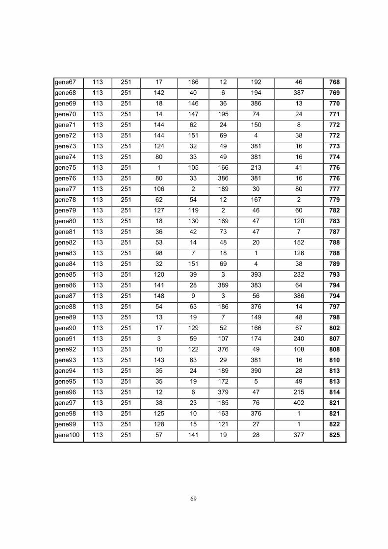
50

gene67 113 251 17 166 12 192 46 768 gene68 113 251 142 40 6 194 387 769 gene69 113 251 18 146 36 386 13 770 gene70 113 251 14 147 195 74 24 771 gene71 113 251 144 62 24 150 8 772 gene72 113 251 144 151 69 4 38 772 gene73 113 251 124 32 49 381 16 773 gene74 113 251 80 33 49 381 16 774 gene75 113 251 1 105 166 213 41 776 gene76 113 251 80 33 386 381 16 776 gene77 113 251 106 2 189 30 80 777 gene78 113 251 62 54 12 167 2 779 gene79 113 251 127 119 2 46 60 782 gene80 113 251 18 130 169 47 120 783 gene81 113 251 36 42 73 47 7 787 gene82 113 251 53 14 48 20 152 788 gene83 113 251 98 7 18 1 126 788 gene84 113 251 32 151 69 4 38 789 gene85 113 251 120 39 3 393 232 793 gene86 113 251 141 28 389 383 64 794 gene87 113 251 148 9 3 56 386 794 gene88 113 251 54 63 186 376 14 797 gene89 113 251 13 19 7 149 48 798 gene90 113 251 17 129 52 166 67 802 gene91 113 251 3 59 107 174 240 807 gene92 113 251 10 122 376 49 108 808 gene93 113 251 143 63 29 381 16 810 gene94 113 251 35 24 189 390 28 813 gene95 113 251 35 19 172 5 49 813 gene96 113 251 12 6 379 47 215 814 gene97 113 251 38 23 185 76 402 821 gene98 113 251 125 10 163 376 1 821 gene99 113 251 128 15 121 27 1 822 gene100 113 251 57 141 19 28 377 825

69