topographic mapping of dissimilarity datasets · fakult¨at f¨ur mathematik/informatik und...
TRANSCRIPT

Topographic Mapping of Dissimilarity Datasets
Dissertationzur Erlangung des Grades einesDoktors der Naturwissenschaften
vorgelegt von
Alexander Hasenfuß
genehmigt von derFakultat fur Mathematik/Informatik und Maschinenbau
der Technischen Universitat Clausthal
Tag der mundlichen Prufung22. September 2009

Die Arbeit wurde angefertigt am Institut fur Informatik an der Technischen Uni-versitat Clausthal.
Dekan der Fakultat: Prof. Dr. J. Dix
Berichterstatterin Prof. Dr. B. Hammer
Mitberichterstatter Prof. Dr. M. Verleysen
Prof. Dr. Th. Villmann

Abstract
A great challenge today, arising in many fields of science, is the proper mappingof datasets to explore their structure and gain information that otherwise wouldremain concealed due to the high-dimensionality. This task is impossible withoutappropriate tools helping the experts to understand the data. A promising wayto support the experts in their work is the topographic mapping of the datasetsto a low-dimensional space where the structure of the data can be visualized andunderstood.
This thesis focuses on Neural Gas and Self-Organizing Maps as particularlysuccessful methods for prototype-based topographic maps. The aim of the thesisis to extend these methods such that they can deal with real life datasets whichare possibly very huge and complex, thus probably not treatable in main memory,nor embeddable in Euclidean space. As a foundation, we propose and investigate afast batch scheme for topographic mapping which features quadratic convergence.This formulation allows to extend the methods to general non-Euclidean settingsin two ways, on the one hand by restricting prototype locations to data points,leading to so-called median variants. On the other hand, continuous prototypeupdates become possible by means of an equivalent formulation of the methodsin terms of pairwise dissimilarities only and the notation of generalized relationalprototypes, leading to so-called relational variants. Since the methods rely on thestandard cost functions of Neural Gas and Self-Organizing Maps (in the version ofHeskes), further extensions to incorporate auxiliary information in terms of labels,and to control the magnification exponent of the resulting prototype distributionbecome possible. The dependency of the models on prototypes allows to include anintuitive patch processing scheme which turns the basic algorithms into a frameworkwhich requires only constant memory and linear time complexity also for the caseof general (quadratic) dissimilarity matrices. The suitability of these methods isdemonstrated in several experiments including an application to text data for whichthe dissimilarity matrix requires almost 250 GB storage capacity.
3

To Baba,with love and thanks

Acknowledgements
I would like to thank my supervisors Barbara Hammer and Thomas Villmann forsimply being the best. I am deeply grateful to them for all.
No love, no friendship can cross the path of our destinywithout leaving some mark on it forever.
– Francois Mauriac (1885 - 1970)
i


Contents
1 Introduction 1
2 Introduction to Topographic Mapping 52.1 Prototype-based Methods . . . . . . . . . . . . . . . . . . . . . . . . 72.2 Self-Organizing Maps . . . . . . . . . . . . . . . . . . . . . . . . . . . 82.3 Topology Representing Networks . . . . . . . . . . . . . . . . . . . . 132.4 The Neural Gas Algorithm . . . . . . . . . . . . . . . . . . . . . . . 142.5 The Magnification Effect . . . . . . . . . . . . . . . . . . . . . . . . . 16
3 Fast Topographic Mapping of Euclidean Data 193.1 Batch Processing for Prototype-based Methods . . . . . . . . . . . . 193.2 Magnification Control for Batch Methods . . . . . . . . . . . . . . . 243.3 Incorporating Additional Information . . . . . . . . . . . . . . . . . 273.4 Processing of Very Large Datasets . . . . . . . . . . . . . . . . . . . 303.5 Experimental Results and Applications . . . . . . . . . . . . . . . . . 32
4 Topographic Mapping of Dissimilarity Data 554.1 Introduction to Dissimilarity Data . . . . . . . . . . . . . . . . . . . 554.2 Prototype-based Methods in Non-Euclidean Spaces . . . . . . . . . . 594.3 Continuous Prototype Updates . . . . . . . . . . . . . . . . . . . . . 664.4 Magnification Control for Relational Methods . . . . . . . . . . . . . 754.5 Processing of Very Large Dissimilarity Datasets . . . . . . . . . . . . 764.6 Experimental Results and Applications . . . . . . . . . . . . . . . . . 79
5 Summary and Outlook 99
References 103
iii


Chapter 1
Introduction
In many fields of science today, massive datasets are collected that have to be exam-ined. A task that is utterly impossible without appropriate automated tools helpingthe experts to understand the data. For example in biomedical sciences, climate re-search, experimental physics, astronomical research, or life sciences, obtained datahas to be grouped, arranged, and illustrated to make it accessible for visual ex-ploration (Keim et al., 2008; Simoff et al., 2008). A promising way to support theexperts in their work is the topographic mapping of the datasets to a low-dimensionalspace where the structure of the data can be visualized and understood. Moreover,those automated tools should present an interpretable visualization of prototypicaldata points to the experts. Then the experts can better control the exploration ofthe data space in the framework of an interactive tool, initiate further experimentswith different settings based on their experience, or manually classify the data tointegrate expert knowledge to the system, for instance.
These requirements are in a perfect way satisfied by prototype-based methodslike Neural Gas and Self-Organizing Maps. Numerous successful applications ofthose methods have been reported in literature as, for instance, substantiated bythe extensive collection of over 7000 references in the Bibliography of Self-OrganizingMap (SOM) Papers (Kaski et al., 1998; Oja et al., 2003; Polla et al., 2007).
Beyond that, a particular challenge in visual analytics is the handling of largedatasets, since especially in this case it is difficult to provide the results in a reason-able time. Unfortunately, the standard formulations of Neural Gas and SOMs arebased on a learning scheme featuring a rate of convergence that is not sufficient fora fast adaptation of the prototypes. Therefore, a fast processing scheme for NeuralGas and SOMs is introduced in the first part of this thesis that accelerates the con-vergence considerably. In addition, useful extensions for the accelerated variantsare presented, which incorporate supplementary information about data into thelearning process, actively control the learning process with regard to the prototypedistribution, and handle even much bigger datasets.
Up to now, we were discussing prototype-based methods which operate in Eu-clidean spaces. But in modern science today, it has become beneficial to applyspecial metrics to measure the pairwise proximities between the objects being re-garded, since Euclidean representations were found to be not descriptive enough tomap the whole structure of the data. Examples for non-Euclidean measures are,for instance, alignment distances from bioinformatics, normalized compression dis-tance from algorithmic information theory, or geodesic distances from graph theory.These special suited dissimilarity measures yield very powerful representations, butin general they originate from non-Euclidean spaces, hence no vector representa-
1

2 Chapter 1 : Introduction
tion is available to work with. The application of the popular standard methodsk-Means, Neural Gas and Self-Organizing Maps that operate in Euclidean spaces istherefore not possible.
A couple of mining tools for non-Euclidean datasets have been proposed: First ofall, the popular kernel approach that has gained a lot of attention in the last decade.By linearizing non-linearities in a kernel-defined feature space, these methods canhandle various complex structured data (Filippone et al., 2008). Kernel functionsproposed for complex structured data are, for instance, Edit distance-based ker-nel functions for strings and graphs (Neuhaus and Bunke, 2006), Fisher Kernel(Saunders et al., 2003) and String Kernel (Lodhi et al., 2002) for text processing,Graph Kernel (Kashima et al., 2004; Bach, 2008), Kernel on pointsets (Parsanaet al., 2008), and Alignment Kernel from bioinformatics (Qiu et al., 2007). Later onin this thesis, we will demonstrate that our proposed prototype-based algorithmscan easily be kernelized and hence are able to make use of the large collection ofavailable kernel functions.
Another popular approach working on dissimilarity data is based on Determin-istic Annealing (Rose, 1998) that was utilized for clustering by Hofmann and Buh-mann (1999), and for a stochastic formulation of Self-Organizing Maps by Graepeland Obermayer (1999).
All these approaches have some drawbacks regarding their applicability for theinterpretable visualization of data: Either they do not provide interpretable out-comes, need too much computational efforts, work only on special classes of dissim-ilarity data, or provide unstable results. But by now there are no simple, robust,and efficient methods for arbitrary dissimilarity datasets.
At this point, the thesis at hand ties up by building the bridge between thestandard prototype-based methods, and the non-Euclidean spaces. An extensionof Neural Gas and Self-Organizing Maps is introduced which can directly work onarbitrary dissimilarity datasets. Since the size of dissimilarity datasets is quadraticin the number of datapoints, these extended methods are also quadratic in theirbasic form and thus they are not applicable to huge datasets. Therefore, we pro-pose a fast and intuitive processing scheme with a linear time and constant spacecomplexity which constitutes one of the few prototype-based methods for very largedissimilarity datasets.
In the first part of the thesis, we lay the technical foundation of the thesis andpresent the standard prototype-based methods. We introduce a fast processingscheme and show its convergence. Furthermore, we propose extensions to incorpo-rate supplementary information about data into the learning process, to activelycontrol the learning process with regard to the prototype distribution, and to handlevery large or streaming datasets using constant memory.
The second part of the thesis deals with dissimilarity data and how to reformu-late the prototype-based methods to work directly on these kind of data. A firstdirect approach is built on the formal notion of cost functions by restricting theflexibility of prototype locations. As an alternative, full flexibility can be achievedby the so-called relational prototypes. We first discuss how to define these proto-types in non-vectorial spaces. Then, based on the possibility to express distancesbetween relational prototypes and data points by only the given dissimilarities be-tween data points, we derive relational variants of the prototype-based standardmethods. Finally, we introduce an approximation scheme to transfer the efficientpatch processing scheme to the non-Euclidean scenario. We demonstrate its ap-plicability in a real-life setting where around 180.000 data objects are processedcorresponding to a full dissimilarity matrix with a size of 250 gigabytes.

3
Finally, it should be mentioned here that the thesis at hand is based on severalscientific research articles to which the author has contributed in the past four years.The thesis is therefore also meant as an extension and an unified presentation ofthe following articles:
Refereed Journals
• Batch and Median Neural GasCottrell, M., Hammer, B., Hasenfuss, A., and Villmann, T.Neural Networks 19:762–771, 2006
• Magnification Control for Batch Neural GasHammer, B., Hasenfuss, A., and Villmann, T.Neurocomputing 70:1225–1234, 2007
• Patch Clustering for Massive Data SetsAlex, N., Hasenfuss, A., and Hammer, B.Neurocomputing 72:1455–1469, 2009
Edited Books
• Median Topographic Maps for Biomedical Data SetsHammer, B., Hasenfuss, A., and Rossi, F.In Similarity-based Clustering and its Application to Medicine and BiologySpringer, 2009
Refereed Conferences
• Magnification Control in Relational Neural GasHasenfuss, A., Hammer, B., Geweniger, T., and Villmann, T.In Proceedings of the 16th European Symposium on Artificial Neural Networks(ESANN 2008), pp. 325–330, 2008
• Patch Relational Neural Gas - Clustering of Huge Dissimilarity DatasetsHasenfuss, A., Hammer, B., and Rossi, F.In Artificial Neural Networks in Pattern Recognition (ANNPR 2008)Springer LNCS 5064:1–12, 2008
• Topographic Processing of Very Large Text Datasets.Hasenfuss, A., Boerger, W., and Hammer, B.In Proc. ANNIE 2008, 2008.
• Single Pass Clustering and Classification of Large Dissimilarity DatasetsHasenfuss, A., and Hammer, B.In Artificial Intelligence and Pattern Recognition (AIPR 2008)pp. 219–223, 2008
• Relational Topographic MapsHasenfuss, A., and Hammer, B.In Advances in Intelligent Data Analysis VII, Proc. IDA 2007Springer LNCS 4723:93–105, 2007
• Neural Gas Clustering for Dissimilarity Data with Continuous PrototypesHasenfuss, A., Hammer, B., Schleif, F.-M., and Villmann, T.In Computational and Ambient Intelligence (IWANN 2007)Springer LNCS 4507:539–546, 2007

4 Chapter 1 : Introduction
• Thinning Mesh AnimationsWinkler, T., Drieseberg, J., Hasenfuss, A., Hammer, B., and Hormann, K.In Proceedings of Vision, Modeling, and Visualization (VMV 2008), 2008
• Relational Neural GasHammer, B., and Hasenfuss, A.In KI 2007: Advances in Artificial IntelligenceSpringer LNAI 4667:190–204, 2007
• Topographic Processing of Relational DataHammer, B., Hasenfuss, A., Rossi, F., and Strickert, M.In Proceedings of 6th Int. Workshop on Self-Organizing Maps (WSOM 2007)
• Intuitive Clustering of Biological DataHammer, B., Hasenfuss, A., Schleif, F.-M., Villmann, T., Strickert, M., andSeiffert, U., In Proceedings of International Joint Conference on Neural Net-works (IJCNN 2007), pp. 1877–1882, 2007
• Accelerating Relational Clustering Algorithms with Sparse Prototype Repre-sentation, Rossi, F., Hasenfuß, A., and Hammer, B.In Proceedings of 6th Int. Workshop on Self-Organizing Maps (WSOM 2007)
• Magnification Control for Batch Neural GasHammer, B., Hasenfuß, A., and Villmann, T.In Proceedings of the 14th European Symposium on Artificial Neural Networks(ESANN 2006), pp. 7–12, 2006
• Supervised Batch Neural GasHammer, B., Hasenfuss, A., Schleif, F.-M., and Villmann, T.In Artificial Neural Networks in Pattern RecognitionSpringer LNAI 4087:33–45, 2006
• Supervised Median ClusteringHammer, B., Hasenfuss, A., Schleif, F.-M., and Villmann, T.In Proceedings of the Artificial Neural Networks in Engineering Conference(ANNIE 2006) 16:623–632, 2006
• Batch Neural GasCottrell, M., Hammer, B., Hasenfuß, A., and Villmann, T.In Proceedings of the 5th Int. Workshop on Self-Organizing Maps (WSOM2005)pp. 275–282, 2005
Chapter 2
Introduction to TopographicMapping
A great challenge today, arising in many fields of science, is the proper mapping ofdatasets to explore their structure and gain information that otherwise would re-main concealed, buried due to the high-dimensionality of the data. In this chapterwe are concerned with the principles of topographic mapping that provides solutionsto this problem.
Usually, a topographic mapping is defined between a high-dimensional inputspace and a low-dimensional map space. The mapping is expected to preserveneighbourhoods to a considerable extent, that is neighbourhoods from input spaceshall be mapped to neighbourhoods in map space, and vice versa. This informaldescription may be sufficient for the present to follow the discussion, later on weshall discuss a more formal framework.
Since the map space is low-dimensional, the mapped data can be visualized eas-ier and often explored better than in the original space. Moreover, the map spaceoften contains a discrete map structure on which the input data is mapped whatleads to particular comfortable and plastic visualizations.
We start by considering some very popular projection techniques that do notexactly focus on a topology-preserving mapping of data but nevertheless shall givea first impression of how data can be projected — and last but not least they arepresented here for historical reasons.
Principal Component Analysis One of the most popular and successful pro-jection technique today is surely the Principal Component Analysis (PCA) thatdates back to the early work of Pearson (1901) and Hotelling (1933). As the namesuggests, PCA’s objective is to determine the most important directions of a givenEuclidean dataset in terms of the variance. The method is based on a linear projec-tion to a subspace using the covariance matrix of data as the linear function thatmaps data to the corresponding subspace spanned by its eigenvectors. That way,the variance of the dataset is optimally preserved by the mapping.
Naturally, by further projecting to the subspace spanned by only a few eigen-vectors corresponding to the largest eigenvalues, one gets the desired dimensionreduction. Note that in this way also the pairwise distances between the datapoints are preserved as good as possible in the projection (cf. Gower, 1966). PCAcan also be linked to the field of neural networks, where Oja’s rule (Oja, 1982, 1992,2008) is a mathematical formalization of Hebbian learning for a single neuron that
5
6 Chapter 2 : Introduction to Topographic Mapping
was shown to perform a principal component analysis on the input data after con-vergence. The converged neuron projects input data to the subspace spanned bythe largest eigenvector of the covariance matrix.
Obviously, the drawback of PCA is its linearity. PCA is not able to providetopology-preserving maps for non-linear datasets and is therefore not suited for to-pographic mapping. Most of the times one will end up with meaningless resultsafter projecting non-linear data — a situation that practitioners usually face whenmessing around with real data. Despite this fact, PCA enjoys great popularity inpractice as attested by the numerous publications of the last 40 years from variousfields, for an overview see e.g. (Jolliffe, 2002).
A generalization of PCA that overcomes the limitations of linearity are the Prin-cipal Curves and Principal Surfaces which provide approximations of data manifoldsby parameterized smooth curves and surfaces (Hastie, 1984; Hastie and Stuetzle,1989). The projection of the data onto the parametric curve or surface is thebest approximation in sense of the mean squared error. Unfortunately, there is nogeneral method to learn the parametric representation of higher dimensional data(Chang and Ghosh, 1999). The original definition of Principal Surfaces has alsolimitations, e.g. problems with self-intersecting data, for an overview see (Ozertem,2008). Chang and Ghosh (2001) proposed a unifying probabilistic model that over-comes several issues.
Multidimensional Scaling In contrast to PCA where vectorial data from aEuclidean space is given, the Multidimensional Scaling (MDS) techniques are con-cerned with pairwise distances between data objects. Their objective is to findsuitable points in a Euclidean space, corresponding to the given pairwise distances,such that those distances are preserved as good as possible by the Euclidean points.Obviously, most of the times some distortion will occur, because in general arbi-trary distances are not isometrically embeddable into Euclidean spaces (Indyk andMatousek, 2004), and even if they are, the dimension of the chosen Euclidean spacemight be too low.
There are many different approaches of MDS, for an excellent overview see (Borgand Groenen, 2005). However, these various variants can be classified into threegroups: Classical Scaling (Torgerson, 1952) the original technique is strongly re-lated to the above introduced PCA as shown by Gower (1966). Essentially, it isa linear model and features the same outcome as PCA when applied to Euclideandistances. Another class is formed by Metric MDS techniques (Torgerson, 1958;Sammon, 1969) which rely on some cost function measuring the distortion error ofthe embedding. These techniques therefore try to preserve the (exact) distances. Incontrast, methods from the third class, the Non-Metric MDS techniques (Kruskal,1964), do not focus on the distances itselves they rather try to keep the ranking ofdistances.
Once again, the focus of multidimensional scaling techniques is not explicitlytopology-preservation. Their objectives are preservation of distances or preservationof ranks regarding distances. Nevertheless, sometimes later on in the experimentswe shall rely on MDS to visualize and explore representative objects that are givenonly by their pairwise distances in between.
In the next section, we are concerned with the basics of prototype-based meth-ods. These methods are based on representative prototypes that are located in dataspace with the aim to characterize a given data distribution as good as possible interms of an error measure. Since prototypes can serve as average representativesfor surrounding data points, the prototype-based methods are very intuitive, practi-
2.1 Prototype-based Methods 7
tioners are able to investigate important characteristics of the data in certain regionsof the data space by analyzing the corresponding representatives. All topographicmapping techniques presented later will therefore be based on prototypes. Havingjustified our decision to focus exclusively on prototype-based methods, we will nowgive a brief introduction about what they are. Moreover, we will introduce two im-portant prototype-based methods, namely Self-Organizing Maps and Neural Gas,which shall play a central role throughout the remaining chapters.
2.1 Prototype-based Methods
Throughout this work, we are exclusively concerned with methods relying on rep-resentative prototypes which are situated within data space in a way that theyapproximate a given data distribution best. These prototype-based approaches of-fer very intuitive learning techniques and their outcomes are meaningful in a waythat they can be interpreted and visualized directly. Practitioners like e.g. biol-ogists, medical scientists, or social scientists are often interested in prototypicalindividuals for further analysis which bear characteristical properties of the data.In this spirit, prototype-based approaches are superior to any other technique andthe right tools to choose. This shall be our motivation to concentrate on thesefruitful approaches leaving aside other models.
Historically issues of that kind were dealt with as part of a far more generalframework in quantization theory (Gersho and Gray, 1992). That’s why we willrely on some nomenclature, definitions, algorithms, and results from that field inthe following. However, the objectives in quantization theory are often differentfrom those in machine learning what justifies an independent treatment of the topic.Only the basics can be transferred, the bigger part has to be built on top anew. Avery recommended reading about all the different facets of quantization theory is thesurvey of Gray and Neuhoff (1998). In what follows, we give some basic definitionsborrowed from quantization theory and introduce the concept of prototype-basedrepresentation in conjunction with central definitions.
Regarding the representation of data by prototypes, the quality of the repre-sentation is usually measured in terms of the quantization error that subsumes thequadratic distances of the data to the nearest prototype. More precisely, let thedata be given by a probability distribution over a manifold V ⊆ �d, described bythe probability density function p. Given a finite collection W = (wi)i∈{1,...,n} from�d of representative prototypes, the prototypes are requested to characterize thedata manifold best when measured by the quantization error
Q(W ) =12
n∑i=1
∫V
χi(W, v) · ‖wi − v‖2p(v) dv, (2.1)
where χi(W, v) is one iff v ∈ {x ∈ �d : ‖wi − x‖ = minwj∈W ‖wj − x‖}, and zeroelse. In this context the set of prototypes W is also called a vector quantizer. Notethat once in a while in the theoretical discussion, we shall also consider countablesets of prototypes.
For a finite set of data points V = {v1, v2, . . . , vm}, drawn with respect tothe underlying probability distribution, the quantization error is estimated by theintra-class variance
Q(W ) =12
n∑i=1
m∑j=1
χi(W, vj) · ‖wi − vj‖2, (2.2)

8 Chapter 2 : Introduction to Topographic Mapping
and we shall also refer to the intra-class variance as the (empirical) quantizationerror (Graf and Luschgy, 2002) from now on.
The prototypes induce a Voronoi diagram {Vi(W ) : wi ∈ W} of �d, whereVi(W ) = {x ∈ �d : ‖wi − x‖ = minwj∈W ‖wj − x‖} is the Voronoi region gen-erated by wi ∈ W . By our definition, the points on a shared border of adjacentprototypes belong to all participating prototypes. The Voronoi diagram is a cover-ing of �d, that is ∪wi∈W Vi = �d. Note that the Voronoi region of a prototype isalso called its receptive field for historical reasons.
We further define the winner index s(v, W ) to be
s(v, W ) = argmini
‖wi − v‖, (2.3)
if it is well-defined. If there are different wi with the same distance to v, ties shallbe broken deterministically, e.g. by consulting the natural order of the indices. Hereand elsewhere we shall omit the set of prototypes W in the notation, leaving χi(v)and s(v), when it can be done without ambiguity.
Naturally the question arises how to algorithmically determine an appropriateset of prototypes for given data. In 1957 Lloyd introduced a prototype-based algo-rithm minimizing the quantization error given a finite set of data that is nowadaysone of the most popular methods operating under the name k-means. After ran-domly initializing the prototypes, it determines in every iteration which points arelocated inside the Voronoi region of each prototype and moves the correspondingprototype to the barycenter of those points. These two operations are repeated un-til a stopping criterion holds. Interestingly, the original method was only publishedas a technical report first, the official journal publication follows not until 1982,see (Lloyd, 1982). Meanwhile, numerous extensions and variations of k-means havebeen published, milestones often cited are e.g. a special online variant by MacQueen(1967), a variant particularly efficient for clustering Hartigan and Wong (1979), andk-means with a growing set of prototypes doubling the number in each step by Lindeet al. (1980). All these k-means derivates determine a set of prototypes, but all ofthem share the common drawback that they easily get stuck in local optima of thecost function they try to optimize. Furthermore, closely linked to this disadvantageis their sensitivity to initialization of the prototypes. Thus, they often provide onlysuboptimal solutions in form of prototypes not faithfully representing given data.Later on, we shall introduce alternative methods overcoming these issues.
Having introduced the basic concepts how to represent data by prototypes ininput space, we are now concerned with a first – and perhaps the most popular –prototype-based technique of topographic mapping, the Self-Organizing Map. Therepresentation of data is no longer done only by prototypes situated in input space,the data is mapped to prototypes in a lower dimensional structure hopefully carryingover much topological information.
2.2 Self-Organizing Maps
Motivated by biological self-organization processes that emerge in neural cell struc-tures, Kohonen (1982, 2001) introduced the concept of Self-Organizing Maps (SOM),modeled as a special artificial neural networks in conjunction with a heuristicallearning rule. Essential part of the concept is the map, a finite structure with afixed topology whose elements shall serve as representatives of the data later on. The

2.2 Self-Organizing Maps 9
term self-organization refers to the ability of the method to reorganize its initial mapand adapt it to the topological characteristics of given input data autonomously.Each element of the map is assigned to a prototype located in input space whichis updated in a vector quantization style but under influence of the neighbourhoodstructure dictated by the map. Those assignments provide the connections betweeneach element of the map and a corresponding Voronoi region of the input space. Bytransferring collective properties of the data within the Voronoi regions in form ofe.g. labels, elements of the map can reflect characteristics of certain regions of theinput space, providing a low-dimensional visualization of high-dimensional data.
Despite its simple and intuitive principle, the Self-Organizing Map has showna robust performance in practice and has proved to be well-suited for many appli-cations. It has raised great interest in different communities and started a largeflow of successive literature. For an extensive collection of over 7000 references seee.g. the Bibliography of Self-Organizing Map (SOM) Papers (Kaski et al., 1998; Ojaet al., 2003; Polla et al., 2007).
Note that Self-Organizing Maps can also be interpreted as discrete approxima-tions of Principal Surfaces (cf. page 6) as pointed out by Mulier and Cherkassky(1995). A related concept are the Elastic Nets, see (Willshaw and von der Malsburg,1976; von der Malsburg and Willshaw, 1977; Durbin and Willshaw, 1987), that showsimilar states of convergence but their ordering process is different (Claussen andSchuster, 2002).
As mentioned before, the Self-Organizing Map is based on a predefined mapstructure with a fixed topology. We refer to this structure in the following as alattice. The lattice is usually chosen as a simple, low-dimensional structure, like arectangular grid, a torus, or a hexagonal grid, to keep the advantage of easy visu-alization. Also more advanced structures like periodical grids in hyperbolic spacefeaturing an exponential growth of elements are sometimes considered (cf. Ritter,1999) but require proper visualization techniques for non-Euclidean structures.
Besides grids also other shapes are possible as lattice structures, e.g. trees areused in the TreeSOM approach (Sauvage, 1997). The lattice can also grow duringprocessing, see the Growing SOM (Bauer and Villmann, 1997) and the GrowingHierarchical Tree SOM (Forti and Foresti, 2006).
The lattice structure needs not to be constructed explicitly for training. Weonly need to know the pairwise distances between the lattice elements induced bythe neighbourhood structure. Here, usually the shortest path distance is chosen,i.e. the shortest path length in a graph-theoretical sense where every arc often haslength one by definition.
More precisely, abstracting from any biological and neural point of view, wedescribe the Self-Organizing Map method as follows:
Formal Description of Self-Organizing Maps
Assume that there is input data given by a probability distribution over a manifoldV ⊂ �d that is described by a probability density function p. As a first ingredient,we introduce a finite collection of prototypes W = (wi)i∈{1,...,n} from �d that servesas a vector quantizer in input space. The second component is a lattice structurefeaturing the same number of elements as W . We identify the elements of the latticestructure with the prototypes of W and denote them also as w1, w2, . . . , wn, whatcan be done formally by a bijective mapping. In doing so, each prototype is in away distinctly connected to an element of the lattice, and vice versa. Since we areonly interested in the pairwise distances of lattice elements, let g(wi, wj) denote thepairwise distance of elements wi and wj in the given lattice structure.
10 Chapter 2 : Introduction to Topographic Mapping
One can imagine the training process of the method as a simultaneous vectorquantization and non-linear projection of the sampled input data whereas bothtechniques influence each other coupled by the connection of prototypes and latticeelements. More formally, the online training algorithm of a Self-Organizing map isgiven as follows:
Training of Self-Organizing Maps The prototypes W = (wi)i∈{1,...,n} fromRd are initialized randomly in input space and are updated in each epoch by therule
Δwi = εt · hλ(g(ws(v), wi)) · (v − wi) (2.4)
for all prototypes wi ∈ W . Thereby, g(·, ·) denotes the pairwise distances in thelattice and ws(v) denotes the winning prototype for the sampled data point v asdefined in (2.3). The parameter λ > 0 controls the neighbourhood range throughthe neighbourhood function hλ(x) = exp(−x/λ). The update is governed by adecreasing step size εt ∈ (0, 1] that usually obeys the condition
∑∞t=1 εt = ∞ and∑∞
t=1 ε2t < ∞, following the work of Robbins and Monro (1951) who introduced
similar conditions in their work on stochastic approximation.During processing the initially large neighbourhood range λ is driven asymptot-
ically to zero changing the characteristics of the updates in every step.
In what follows, we intent to give a brief summary of the theoretical propertiesthat were derived for Self-Organizing Maps. Unfortunately, despite its algorithmicsimplicity and intuitivity, the method has shown to be quite resistant against amathematical treatment. For an overview of the latest achievements see (Cottrellet al., 1994, 1998; Hammer and Villmann, 2003; Fort, 2006). Briefly, the state-of-the-art is a broad theoretical understanding of the one-dimensional case but onlyfew theoretical results about the multi-dimensional case are known.
Theoretical Properties of Self-Organizing Maps Due to the dynamics ofλ, the Self-Organizing Maps show two phases during training (cf. Sadeghi, 2001).In a first phase, the self-organization phase, the initially disordered prototypes andtherefore also the disordered map elements become in some way organized reflectingtopological properties of the input space. In the second phase, the convergencephase, the prototypes converge to their final destinations driven in a fashion ofa special case of the Robbins-Monro algorithm (cf. Sadeghi, 1998), but for finitedatasets they do not minimize exactly the quantization error as pointed out byRynkiewicz (2006) based on previous work by Fort and Pages (1995, 1996).
However, it must be stated here that almost all theoretical results about SOMwere derived only for the one-dimensional case, i.e. one-dimensional input spaceand a one-dimensional lattice in shape of a chain. These results transfer also tosettings where lattice space and data space are separable, i.e. the distributions areindependent for each dimension. There is not much theoretical evidence about thegeneral multidimensional case. Complete proofs of convergence in the general caseare not known so far.
Moreover, it has been shown that in general for a continuous input distributionthere does not exist any cost function that is minimized by the Self-Organizing Mapin a gradient descent fashion (cf. Erwin et al., 1992).
Heskes and Kappen (1993); Heskes (1996, 1999) demonstrated for the generalcase that by slightly changing the winner definition in the update rule (2.4), nom-inating a prototype as winner that minimizes the weighted average distance (also

2.2 Self-Organizing Maps 11
referred to as the local error) to the sampled data point instead, that is
s∗(v, W ) =n
argmini=1
n∑k=1
hλ(g(wi, wk))‖wk − v‖2 , (2.5)
the modified Self-Organizing Map performs a stochastic gradient descent on thecost function
ESOM(W ) =12
n∑i=1
∫hλ(g(ws∗(v), wi)) · ‖wi − v‖2
p(v) dv. (2.6)
Finishing this brief summary of the theoretical properties of SOM, it should bementioned here that despite the lack of theoretical evidence Self-Organizing Mapsperform very robust and reliable in practical applications, surely one good reasonfor their popularity in numerous fields (Kohonen, 2001).
It should also be noted that Bishop et al. (1998a,b) proposed a concurrentmethod, the Generative Topographic Mapping (GTM). GTM is a probability den-sity model which describes the data distribution by latent variables utilizing a gridin a low dimensional latent space and a set of non-linear basis functions that arecombined in data space governed by an adapted transformation. The model is aprobabilistic reformulation of Kohonen’s SOM appropriate to overcome disadvan-tages of the Self-Organizing Map. The GTM model comes up with an explicitcontinuous density model of the input data not only a discrete one as in case ofSOM, a provable convergence in contrast to SOM, and a cost function signalizingthe quality of the map. Nevertheless, a decade after its introduction the GTM hasnot yet displaced the original Self-Organizing Map, maybe owing to its less intuitiveprinciple. The intention of our thesis is topographic mapping by prototype-basedmethods, so we leave it at that brief discussion of GTM.
In the following section, we are concerned with the topology preservation prop-erty of Self-Organizing Maps, a crucial aspect regarding the visualization ability ofa projection method.
Topology Preservation in Self-Organizing Maps
One of the most important issues concerning SOM is the topology preservationfeature that is needed for a meaningful projection of (intrinsic) high-dimensionalinput data into the lower-dimensional lattice space. Since in general the projectionwill take place from a higher to a true lower-dimensional space, naturally sometopological information will be lost in the process due to disrupted neighbourhoods,or new neighbourhoods will be created where there were none before. This is usuallyreferred to as the dimension conflict. But also a mismatch in the topology of datamanifold and the fixed lattice structure will impose errors. As discussed by Vennaand Kaski (2006) these kinds of errors influence the measures trustworthiness anddiscontinuity of the map. Obviously, there is a tradeoff between those measures,thus projection methods cannot optimize both objectives at the same time.
For analyzing the quality of the mapping in terms of topology preservation, onehas to define appropriate measures in a mathematically sound way. This issue isnot trivial, there were various formal frameworks proposed measuring the topologypreservation of a Self-Organizing Map, for a comprehensive overview see (Baueret al., 1999; Villmann, 2004). The most promising approach is the topographicproduct (Bauer and Pawelzik, 1992) defined on rectangular and hexagonal lattice
12 Chapter 2 : Introduction to Topographic Mapping
structures and the more general topographic function (Villmann et al., 1997; Vill-mann, 1997).
In the context of Self-Organizing Maps, we can formally define a topology pre-serving mapping as a pair of suitable forth and back mappings between data andlattice space that are both continuous in the topological sense, i.e. they are neigh-bourhood preserving. If a topology preserving mapping between a data manifoldand a lattice structure exists, we call the lattice a topology preserving map of themanifold. Later on, we will also refer to this kind of lattice as a perfectly topol-ogy preserving map to emphasize its ultimate perfection in contrast to topographicmaps with some topological defects that shall be discussed later. For a formal dis-cussion of topology preservation we need to define suitable neighborhoods on dataand lattice spaces to obtain topological spaces.
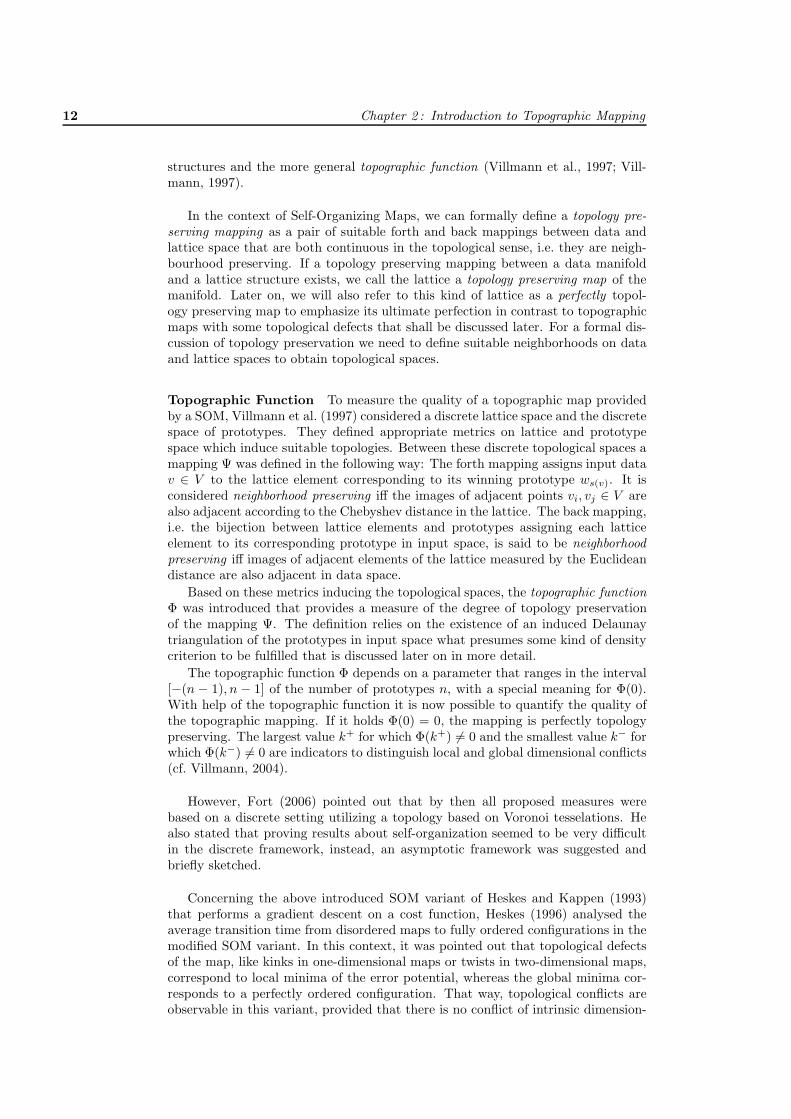
Topographic Function To measure the quality of a topographic map providedby a SOM, Villmann et al. (1997) considered a discrete lattice space and the discretespace of prototypes. They defined appropriate metrics on lattice and prototypespace which induce suitable topologies. Between these discrete topological spaces amapping Ψ was defined in the following way: The forth mapping assigns input datav ∈ V to the lattice element corresponding to its winning prototype ws(v). It isconsidered neighborhood preserving iff the images of adjacent points vi, vj ∈ V arealso adjacent according to the Chebyshev distance in the lattice. The back mapping,i.e. the bijection between lattice elements and prototypes assigning each latticeelement to its corresponding prototype in input space, is said to be neighborhoodpreserving iff images of adjacent elements of the lattice measured by the Euclideandistance are also adjacent in data space.
Based on these metrics inducing the topological spaces, the topographic functionΦ was introduced that provides a measure of the degree of topology preservationof the mapping Ψ. The definition relies on the existence of an induced Delaunaytriangulation of the prototypes in input space what presumes some kind of densitycriterion to be fulfilled that is discussed later on in more detail.
The topographic function Φ depends on a parameter that ranges in the interval[−(n − 1), n − 1] of the number of prototypes n, with a special meaning for Φ(0).With help of the topographic function it is now possible to quantify the quality ofthe topographic mapping. If it holds Φ(0) = 0, the mapping is perfectly topologypreserving. The largest value k+ for which Φ(k+) �= 0 and the smallest value k− forwhich Φ(k−) �= 0 are indicators to distinguish local and global dimensional conflicts(cf. Villmann, 2004).
However, Fort (2006) pointed out that by then all proposed measures werebased on a discrete setting utilizing a topology based on Voronoi tesselations. Healso stated that proving results about self-organization seemed to be very difficultin the discrete framework, instead, an asymptotic framework was suggested andbriefly sketched.
Concerning the above introduced SOM variant of Heskes and Kappen (1993)that performs a gradient descent on a cost function, Heskes (1996) analysed theaverage transition time from disordered maps to fully ordered configurations in themodified SOM variant. In this context, it was pointed out that topological defectsof the map, like kinks in one-dimensional maps or twists in two-dimensional maps,correspond to local minima of the error potential, whereas the global minima cor-responds to a perfectly ordered configuration. That way, topological conflicts areobservable in this variant, provided that there is no conflict of intrinsic dimension-

2.3 Topology Representing Networks 13
ality in principle.
As discussed above, one serious drawback of Self-Organizing Maps is their fixedlattice structure that is very well suited for visualization but lacks of flexibilityin terms of topology. Another type of methods trades easy visualization in fora more flexible lattice structure that is driven by data and not fixed beforehand.The approach is based on so called Topology Representing Networks which shall bediscussed in the following section.
2.3 Topology Representing Networks
In this section, we briefly introduce a topographic mapping approach (Martinetzand Schulten, 1994) that in contrast to Self-Organizing Maps does not depend ona predefined fixed lattice structure. It constructs its lattice structure according tothe given data topology by applying a competitive Hebbian scheme.
More precisely, let M ⊆ �d be a manifold which we suppose for the present to begiven explicitly. Suppose further that there is a finite collection of prototypes W =(wi)i∈{1,...,n} from �d lying in the manifold. We shall show later how prototypes can
be distributed homogeneously over a manifold. We name V(M)i (W ) = Vi(W ) ∩ M
the masked Voronoi region of prototype wi. Because of wi ∈ M and of course wi ∈Vi(W ) the intersection is never empty. Moreover, since the Voronoi diagram V (M)covers �d, the masked Voronoi diagram covers M , i.e. it is M =
⋃ni=1 V
(M)i (W ).
We define a neighbourhood relation of prototypes on the manifold by a non-empty intersection of the corresponding masked Voronoi regions. That way, amasked Voronoi diagram generates a so-called induced Delaunay triangulation, agraph structure on W that is given by the adjacency of the masked Voronoi re-gions, i.e. there is an edge wi
e wj iff V(M)i (W ) ∩ V
(M)j (W ) �= ∅. As shown by
Martinetz and Schulten (1994, Theorem 2), the induced Delaunay triangulation isa perfectly topology preserving map of M . That means, neighbourhoods in themanifold are mapped to neighbourhoods in the graph structure, and vice versa. Itis to be understood here, that obviously the larger the number of prototypes thefiner is the resolution of the map. Note that by definition, also one single prototypewi ∈ M is a perfectly topology preserving map!
At this point the question arises how to determine the induced Delaunay tri-angulation algorithmically. This is not as easy as the construction of the standardDelaunay triangulation via the Voronoi regions. Usually, the manifold M is onlyaccessible by a probability distribution defined on �d, i.e. we can only sample itspoints. Martinetz and Schulten (1994) therefore proposed an iterative Hebbianlearning scheme that always strengthen the connections between first and secondwinner prototype for each sampled point.
Martinetz and Schulten (1994) defined prototypes W ⊆ M to be dense in M iffor every v ∈ M the triangle formed by v and the first and second winner prototyperegarding v lies completely in M , i.e. Δvws(v)ws′(v) ⊆ M . For instance, in convexdatasets the prototypes are always dense according to the above definition. More-over, it was shown that the generated connective structure of a TRN converges tothe induced Delaunay triangulation if the prototypes are lying dense in the man-ifold. The resulting graph structure was also shown to be path-preserving in themanifold M , i.e. two points wi, wj are connected by a path in the graph structureif and only if they are connected by a path in the manifold M .1
1A path in a manifold X from x1 to x2 is a continuous map φ : [a, b]→ M such that φ(a) = x1
and φ(b) = x2.

14 Chapter 2 : Introduction to Topographic Mapping
Thus, under the constraint that the prototypes obey a density criterion regardingthe underlying data manifold, applying a competitive Hebbian scheme by alwaysconnecting the first and second ranked prototypes leads to a graph structure thatrepresents the induced Delaunay triangulation of the data manifold. That way, aperfect topology preservation is obtained. The outcoming lattice can be seen as adiscrete, path preserving representation of the data manifold. In this context, wecall that approach a topology representing network.
Martinetz and Schulten (1994) discussed loosely in this context that a homo-geneous distribution of prototypes can be made dense by increasing the number ofprototypes. Obviously, if the data manifold M has a smooth boundary ∂M , e.g.it is convex, a sufficiently large number of prototypes will be dense in M . Notethat this aspect is of great importance for the algorithmic usage, later on we willpresent a technique capable of generating a homogeneous distribution of prototypesand therefore constituting the foundation of the discussed approach.
It should be noted here that there is a related framework introduced by Fritzke(1995) and Bruske and Sommer (1995) which relies on a growing strategy. Thenumber of prototypes is increased by time and topological connections are drawnusing the same Hebbian scheme as above. Connections as well as prototypes fadeaway during the iteration process if they no longer match the topology best. Lateron Fritzke (1997) applied his approach also successfully to the processing of non-stationary distributions. For some of the latest developments in this direction,namely the Growing Hierarchical Tree SOM, see also (Forti and Foresti, 2006).
One important question concerning the usability of the Topology RepresentingNetwork approach has remained open: We haven’t discussed yet how to get suit-able prototypes lying in the manifold and capturing the subtleties of the topology.Fortunately, there is a reliable vector quantization technique distributing its proto-types exactly as desired, the so-called Neural Gas method. In what follows we willintroduce the principles of Neural Gas.
2.4 The Neural Gas Algorithm
As motivated in the last section, the foundation of Topology Representing Net-works are prototypes which lie dense in the data manifold. As stated by Martinetzand Schulten (1994), a homogeneous distribution of prototypes can always be madedense by simply increasing the number of prototypes. For that reason, methods aresought after that are capable of distributing prototypes homogeneously in the datamanifold. In the following, we will present the very robust and reliable vector quan-tization method Neural Gas that can serve as a basis for Topology RepresentingNetworks (Martinetz and Schulten, 1994). Besides being part of Topology Repre-senting Networks, it also offers great advantage over the popular k-means algorithmand can be used as a substitute (Martinetz et al., 1993).
Neural Gas (NG), introduced by Martinetz et al. (1993), is a vector quantizationtechnique that aims to construct a finite collection W = (wi)i∈{1,...,n} of represen-tative prototypes from �d for a given data manifold M ⊂ �d. Once in a while inthe theoretical discussion, we shall also consider countable sets of prototypes.
In the following, let the data be given by a probability distribution over a man-ifold V ⊆ �d, described by the probability density function p. The prototypes arethen requested to characterize the data manifold best when measured by the quan-tization error (2.1). Technically, Neural Gas utilizes a stochastic gradient descenton a cost function that is based on a ranking scheme, relating the strength of pro-

2.4 The Neural Gas Algorithm 15
totypes updates to their ranks regarding the distances to the sampled data point.Due to its importance for the theory of Neural Gas and all upcoming parts of thiswork, we would like to emphasize the following definition of ranks:
Definition 2.4.1 (Ranking of Prototypes) Let W = (wi)i∈{1,...,n} from �d bea finite collection of prototypes. The rank ki(W, v) of a prototype wi relative to datapoint v ∈ �d is given by the rank function ki :
(�ni=1�
d)×�d→ {0, 1, . . . , n − 1}
defined by
ki(w1, w2, . . . , wn, v) = |{wk : ‖wk − v‖ < ‖wi − v‖}|. (2.7)
Moreover, we require the function to be bijective. If necessary, ties ‖wk − v‖ =‖wi − v‖ shall be broken deterministically. For convenience, we denote also therank function as ki(W, v) in the following. �
We would also like to emphasize the importance of Neural Gas for the thesis athand. It shall serve us as a reference throughout in a way that new techniques areintroduced and discussed on its basis. In the majority of cases, these introducedtechniques are easily transferable to Self-Organizing Maps or k-Means due to theclose relationship between the models. So most of the times, we present only theNeural Gas variant of a technique and settle back by simply referring to the analogyof the procedure. Having set the further course of action, we present the NeuralGas algorithm in the following.
Neural Gas Algorithm
For input data given by a probability distribution that is described by a probabilitydensity function p, Neural Gas performs a stochastic gradient descent on the costfunction
Eλ(W ) =n∑
i=1
∫hλ(ki(W, v)) · ‖wi − v‖2
p(v) dv, (2.8)
through the update rule
Δwi = εt · hλ(ki(W, v)) · (v − wi) (2.9)
for all prototypes wi ∈ W . The parameter λ > 0 controls the neighbourhood rangethrough the neighbourhood function hλ(x) = exp(−x/λ). The update is governedby a decreasing step size εt ∈ (0, 1] that usually obeys the condition
∑∞t=1 εt = ∞
and∑∞
t=1 ε2t < ∞, following the work of Robbins and Monro (1951) who introduced
similar conditions in their work on stochastic approximation.
During processing the initially large neighbourhood range λ is driven asymptot-ically to zero changing the characteristics of the cost function in every step. Dueto the dynamics of λ, Neural Gas is not sensitive to initialization, and most localoptima are supposed to arise only later in the process. Therefore the neighbourhooddynamics prevents the method from getting stuck too early in suboptimal states.Note that for a vanishing neighbourhood range the cost function Eq. (2.8) becomesthe quantization error (2.1), since C(λ) → 1 and hλ(ki(W, v)) → χi(W, v) hold forλ → 0.
For all experiments in this work the initial neighborhood range λ0 was chosenas n/2 as suggested by Martinetz et al. (1993), where n is the number of neuronsused. The neighborhood range λt was decreased exponentially with the number of

16 Chapter 2 : Introduction to Topographic Mapping
adaptation steps t according to λt = λ0 · (0.01/λ0)t/tmax as it was suggested in theoriginal work of Martinetz et al. (1993). The value tmax is the number of epochs ofa training run.
In what follows we are concerned with an inherent but counterintuitive char-acteristic of vector quantizers. The final prototypes do not exactly reproduce theinput data density, instead an asymptotic power law holds. This inherent charac-teristic can pose undesired effects in practical applications and has therefore to bekept in mind while applying vector quantizers.
2.5 The Magnification Effect
It was first demonstrated by Zador (1963, 1982) and stated more precisely by Grafand Luschgy (2000) that vector quantization techniques aiming for a minimizationof the distortion error feature the inherent characteristic that the final prototypedensity � does not exactly match the data density p. Instead, the relation betweenthose densities asymptotically obeys the power law
�(w) ∼ p(w)α, (2.10)
with α �= 1 in general. In this context, the exponent α is called the magnificationexponent. In a more general setting, the magnification characteristic of a certainmethod is called the magnification factor.
The magnification effect might seem counterintuitive at first feel, but it can beeasily observed in experiments when sparsely sampled regions of the input spacewith low probability draw prototypes from dense regions. This is particularly strik-ing in case of outliers in real data.
In general, the magnification effect is an inherent characteristic of the differentmethods and not only vector quantizers suffer from this discrepancy. Although, fora variety of popular methods, the magnification follows a power law with exponentdifferent from one (see Villmann and Claussen, 2006).
As it was shown by Zador (1982) in a more general setting, for vector quantizersminimizing the quadratic distortion error Eq. (2.1), like the popular k-means, itholds
α =d
d + 2, (2.11)
where d denotes the intrinsic data dimensionality (see also Graf and Luschgy, 2000).Martinetz et al. (1993) proved that for a small neighbourhood range 0 < λ n
the Neural Gas algorithm also features a magnification exponent of α = d/(d + 2),what is consistent with the result of Zador (1982) in (2.11).
A magnification factor of one relates to an optimal information transfer andyields maximum entropy of the mapping in an information-theoretical sense. Theprototypes are then exactly adjusted according to the underlying data distribution– the data density equals the prototype density. In that case, the amount of in-formation, which is conserved replacing the points in the receptive fields by theirrepresentative prototypes, is maximized.
It also means that all prototypes have the same probability over the data distri-bution to become winner. For a given data distribution P and magnification factor

2.5 The Magnification Effect 17
one, it then holds
lim|W |→∞
∣∣∣∣∣∫
Vi(W )
v dP (v) −∫
Vj(W )
v dP (v)
∣∣∣∣∣ = 0 for all wi, wj ∈ W ,
where Vi(W ) and Vj(W ) are the corresponding Voronoi regions of the final prototypelocations wi, wj ∈ W after learning, respectively.
A magnification factor one is specific for approaches explicitly optimizing theinformation transfer or related measures (cf. Linsker, 1989).
The reader might be in doubt about the impact of the magnification effect inreal-life data, because for high-dimensional data, Neural Gas is approximately in-formation optimal, since d/(d + 2) → 1 for d → ∞. But almost always the intrinsicdimensionality of real data is very low, i.e. d d. So there is a good justificationto deal with the magnification effect in the real world.
Later on, subsequent to the presentation of each upcoming method, we willdiscuss possibilities to modify the methods in a way that the magnification exponentchanges. That results in an altered distribution of the final prototypes and opensthe field of magnification control allowing for arbitrary control of the magnification.
As discussed above, Neural Gas tends to shift prototypes towards regions wheredata is sparsely sampled. This inherent behaviour might lead to unwanted effectsif, for example, unwanted outliers occur in the dataset (Hodge and Austin, 2004).Here, magnification control can help to suppress the influence of the outlying datapoints.
In practice also the opposite effect is of great interest. For example, if the focuslies on rare events that should be covered by prototypes (Merenyi and Jain, 2004;Villmann et al., 2003; Villmann and Heinze, 2000), magnification control allows toemphasize regions of low density.
In the next chapter, we will discuss how to accelerate the introduced prototype-based methods and also how to apply them efficiently on very large datasets.

18 Chapter 2 : Introduction to Topographic Mapping

Chapter 3
Fast Topographic Mapping ofEuclidean Data
This chapter is concerned with fast variants of prototype-based methods that canbe applied if the given Euclidean dataset is finite. They show a very fast conver-gence compared to the original formulations and can be used as a replacement inall applications where the whole dataset is available in advance. Later on, we willdiscuss also variants that are capable of dealing with very large datasets, and alsowith streaming data or datasets that are gathered over time.
The proofs and concepts in this section shall play an important role for thiswork, because all following parts are based on quite similar reasonings and can betraced back to the proofs and concepts presented here. That’s why we will givemore details here and keep things shorter later on by referencing to this chapter.
3.1 Batch Processing for Prototype-basedMethods
The original Neural Gas method optimizes its cost function by applying a stochasticgradient descent method, that in principle needs many iterations until convergence(Martinetz et al., 1993). However, if a finite dataset {v1, v2, . . . , vm} is given, NeuralGas can be formulated as a faster batch variant as introduced by Cottrell et al.(2005, 2006).
In the finite setting, the cost function of Neural Gas Eq. (2.8) becomes
Eλ(W ) =12
n∑i=1
m∑j=1
hλ(ki(W, vj)) · ‖wi − vj‖2. (3.1)
In every iteration of a batch approach, all prototypes are updated at once takinginto account the whole dataset. The optimal locations of the prototypes musttherefore be calculated in an efficient manner, that’s why we are looking for ananalytic solution.
Obviously,
∂
∂wiEλ(W ) =
∑j
hλ(ki(W, vj))(wi − vj)!= 0
cannot be solved explicitly because of the rank function. As a consequence, thereis no way to directly derive update rules for the optimal prototype locations.
19

20 Chapter 3 : Fast Topographic Mapping of Euclidean Data
For this reason, we introduce a set of hidden variables kij to replace the rankfunction ki(W, vj), where {kij : i ∈ {1, 2, . . . , n}} is a permutation of {0, 1, . . . , n−1} for every j ∈ {1, 2, . . . , m}. This yields
Eλ(W, kij) =12
∑i
∑j
hλ(kij) · ‖wi − vj‖2. (3.2)
That way, an alternating optimization technique (Hathaway and Bezdek, 2003) canbe applied, that, in turn, optimizes the hidden variables kij for fixed prototypelocations wi, and then determines optimal prototype locations wi for fixed hiddenvariables kij , according to the cost function Eq. (3.2).
In Table 3.1 the Batch Neural Gas algorithm is quoted. In the following, we willdiscuss in detail how to get the optimal assignments in each step of the alternatingoptimization. Also a proof of convergence of the algorithm in sense of the costfunction is given.
Algorithm 3.1: Batch Neural Gas
Input
Data V = {v1, v2, . . . , vm} ⊂ �d
Begin
(* Initialize prototypes and neighbourhood range *)
Init wi ∈ �d randomly for all i ∈ {1, . . . , n} and λ0 = n/2, λ = λ0
(* Repeat for a given number of epochs. . . *)
for t := 1 to epochs do
Compute Euclidean distances. . .
d(wi, vj) = ‖wi − vj‖Determine hidden variables as ranks (break ties deterministically). . .
kij = |{ l ∈ {1, . . . , n} : d(wl, vj) < d(wi, vj)}|Update prototype locations. . .
wi =∑
j hλ(kij) · vj/∑
j hλ(kij)
Decrease neighbourhood range. . .
λ = λ0 · (0.01/λ0)t/epochs
endfor;
(* Return representative prototypes *)
Return wi
End.
Optimal Assignments
The first step of the alternating optimization is the determination of optimal as-signments for the hidden variables kij . Given fixed prototype locations, an optimalassignment for the hidden variables kij , in terms of the modified cost function Eλ,turns out to be the ranks of the prototypes, that means
kij = ki(W, vj), (3.3)

3.1 Batch Processing for Prototype-based Methods 21
since that way farther situated prototypes will get lower weights, and vice versa.
Assume W are fixed prototype locations. We say an assignment k′ij is conform
with the ranks ki(W, vj) if there is no pair (k′tj , k
′t′j) with k′
tj < k′t′j and ‖wt − vj‖2
>
‖wt′ − vj‖2. Obviously, kij = ki(W, vj) is conform with the ranks.
Proposition 3.1.1 Let W be fixed prototype locations. Then, the assignmentkij = ki(W, vj) is a global minimizer of Eλ(W, kij), and it is unique up to conformity.
Proof. To verify the claim, we show that all conform assignments are global mini-mizers of Eλ(W, kij), and that it holds Eλ(W, kij) < Eλ(W, k′
ij) for any assignmentk′
ij not conform with the ranks ki(W, vj).
We may assume, without loss of generality, that the fixed prototypes w1, w2, . . . , wn
are subscripted in a way that
‖w1 − vj‖2 ≤ ‖w2 − vj‖2 ≤ . . . ≤ ‖wn − vj‖2
when considering vj . Let t < t′. For any nonnegative η, η′ with η < η′ it then holds
‖wt − vj‖2< ‖wt′ − vj‖2 ⇐⇒
(η′ − η) · ‖wt − vj‖2< (η′ − η) · ‖wt′ − vj‖2 ⇐⇒
η · ‖wt − vj‖2 + η′ · ‖wt′ − vj‖2> η′ · ‖wt − vj‖2 + η · ‖wt′ − vj‖2
(3.4)
Since the set of possible assignments is finite, there must exist a global minimizer,an assignment k∗
ij with Eλ(W, k∗ij) ≤ Eλ(W, kij) for all possible assignments kij .
Let k∗ij be a global minimizer of Eλ for fixed prototypes W . Suppose k∗
ij is notconform with the ranks ki(W, vj). By definition of conformity, there must existat least one pair (k∗
tj , k∗t′j) where k∗
tj > k∗t′j and ‖wt − vj‖2
< ‖wt′ − vj‖2. Let(k∗
tj , k∗t′j) be such a pair and set ηij = hλ(k∗
ij) = exp(−k∗ij/λ). Then, the cost
function can be written as
Eλ(W, k∗ij) =
12
∑j
⎡⎣ ∑
i�=t,i�=t′ηij ‖wi − vj‖2 + ηtj ‖wt − vj‖2 + ηt′j ‖wt′ − vj‖2
⎤⎦ .
Since by assumption k∗ij is not conform with the ranks due to the pair (k∗
tj , k∗t′j),
it holds ηtj < ηt′j and ‖wt − vj‖2< ‖wt′ − vj‖2. Then, according to Eq. (3.4), we
obtain
Eλ(W, k∗ij) >
12
∑j
⎡⎣ ∑
i�=t,i�=t′ηij ‖wi − vj‖2 + ηt′j ‖wt − vj‖2 + ηtj ‖wt′ − vj‖2
⎤⎦
=: Eλ(W, k∗∗ij )
Thus, there is an assignment k∗∗ij with Eλ(W, k∗∗
ij ) < Eλ(W, k∗ij), namely the assign-
ment where positions t and t′ are transposed compared to k∗ij . But then k∗
ij is not aminimizer, what leads to a contradiction. Therefore, the supposition must be false,k∗
ij has to be conform with the ranks. Thus, any global minimizer of Eλ is conformwith the ranks.
Obviously, all conform assignments share the same value when mapped by Eλ.Since there must exist a global minimizer that is always a conform assignment,by definition, all conform assignments are global minimizers of Eλ. In particular,

22 Chapter 3 : Fast Topographic Mapping of Euclidean Data
the assignment kij = ki(W, vj) is a global minimizer of the function Eλ for fixedprototypes, and it is unique up to conformity. �
If ties in the rank determination are broken deterministically, then kij = ki(W, vj)is the only conform assignment, and therefore a unique global minimizer of Eλ(W, kij)for fixed W .
Optimal Prototypes
The second step of the alternating optimization is the determination of optimalprototype locations. It turns out that the optimal prototype locations W for fixedhidden variables kij are given by the update rule
wi =
∑j hλ(kij) · vj∑
j hλ(kij)for all i ∈ {1, 2, . . . , n}. (3.5)
This can be seen as follows: Consider the modified cost function Eλ fromEq. (3.2) with substituted fixed hidden variables. It is differentiable on the wholedomain, and the partial derivatives of this modified cost function are given by
∂
∂wiEλ(W, kij) =
∂
∂wi
12
∑i
∑j
hλ(kij) ‖wi − vj‖2 =∑
j
hλ(kij)(wi − vj)
= wi ·∑
j
hλ(kij) −∑
j
hλ(kij)vj ,
and from∂
∂wiEλ(W, kij)
!= 0 and∑
j hλ(kij) > 0 it follows immediately that critical
points W ∗ are given by
w∗i ·
∑j
hλ(kij) −∑
j
hλ(kij)vj = 0 ⇐⇒ w∗i =
∑j hλ(kij) · vj∑
j hλ(kij).
It is straightforward to verify that the Hessian matrix
H(W, kij) =(
∂2
∂wi∂wjEλ(W, kij)
)i,j∈{1,2,...,n}
is positive definite on the whole domain, because H is a diagonal matrix withpositive diagonal entries
∂2
∂w2i
Eλ(W, kij) =∑
j
hλ(kij) > 0.
Therefore, Eλ is strictly convex on the whole domain, and there exists only onecritical point W ∗ that is a global minimizer of Eλ.
Hence, it follows that the update rule Eq. (3.5) sets the prototypes directly tothe unique global minimum of function Eλ.
Convergence
In the following, it is shown that Batch Neural Gas converges to a local minimumof the cost function Eq. (3.2). The proof is based on the work of Bottou and Bengio(1995).
3.1 Batch Processing for Prototype-based Methods 23
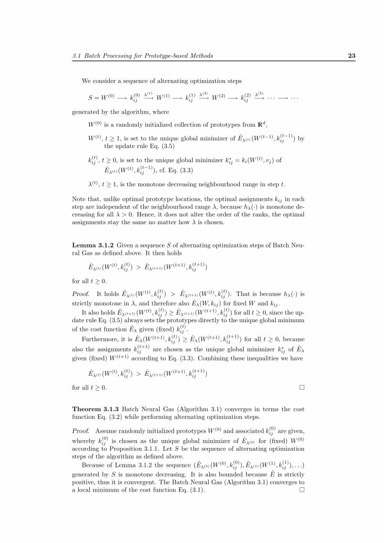
We consider a sequence of alternating optimization steps
S = W (0) −→ k(0)ij
λ(1)−→ W (1) −→ k(1)ij
λ(2)−→ W (2) −→ k(2)ij
λ(3)−→ · · · −→ · · ·
generated by the algorithm, where
W (0) is a randomly initialized collection of prototypes from �d,
W (t), t ≥ 1, is set to the unique global minimizer of Eλ(t) (W (t−1), k(t−1)ij ) by
the update rule Eq. (3.5)
k(t)ij , t ≥ 0, is set to the unique global minimizer k∗
ij = ki(W (t), vj) of
Eλ(t)(W (t), k(t−1)ij ), cf. Eq. (3.3)
λ(t), t ≥ 1, is the monotone decreasing neighbourhood range in step t.
Note that, unlike optimal prototype locations, the optimal assignments kij in eachstep are independent of the neighbourhood range λ, because hλ(·) is monotone de-creasing for all λ > 0. Hence, it does not alter the order of the ranks, the optimalassignments stay the same no matter how λ is chosen.
Lemma 3.1.2 Given a sequence S of alternating optimization steps of Batch Neu-ral Gas as defined above. It then holds
Eλ(t)(W (t), k(t)ij ) > Eλ(t+1)(W (t+1), k
(t+1)ij )
for all t ≥ 0.
Proof. It holds Eλ(t)(W (t), k(t)ij ) > Eλ(t+1)(W (t), k
(t)ij ). That is because hλ(·) is
strictly monotone in λ, and therefore also Eλ(W, kij) for fixed W and kij .It also holds Eλ(t+1)(W (t), k
(t)ij ) ≥ Eλ(t+1)(W (t+1), k
(t)ij ) for all t ≥ 0, since the up-
date rule Eq. (3.5) always sets the prototypes directly to the unique global minimumof the cost function Eλ given (fixed) k
(t)ij .
Furthermore, it is Eλ(W (t+1), k(t)ij ) ≥ Eλ(W (t+1), k
(t+1)ij ) for all t ≥ 0, because
also the assignments k(t+1)ij are chosen as the unique global minimizer k∗
ij of Eλ
given (fixed) W (t+1) according to Eq. (3.3). Combining these inequalities we have
Eλ(t)(W (t), k(t)ij ) > Eλ(t+1)(W (t+1), k
(t+1)ij )
for all t ≥ 0. �
Theorem 3.1.3 Batch Neural Gas (Algorithm 3.1) converges in terms the costfunction Eq. (3.2) while performing alternating optimization steps.
Proof. Assume randomly initialized prototypes W (0) and associated k(0)ij are given,
whereby k(0)ij is chosen as the unique global minimizer of Eλ(0) for (fixed) W (0)
according to Proposition 3.1.1. Let S be the sequence of alternating optimizationsteps of the algorithm as defined above.
Because of Lemma 3.1.2 the sequence (Eλ(0) (W (0), k(0)ij ), Eλ(1)(W (1), k
(1)ij ), . . .)
generated by S is monotone decreasing. It is also bounded because E is strictlypositive, thus it is convergent. The Batch Neural Gas (Algorithm 3.1) converges toa local minimum of the cost function Eq. (3.1). �
24 Chapter 3 : Fast Topographic Mapping of Euclidean Data
As demonstrated by Cottrell et al. (2006), Batch Neural Gas features a quadraticrate of convergence because it is interpretable as a Newton optimization method,in contrast to the simple gradient descent of the original Neural Gas.
Following the same ideas, we can easily derive the Batch SOM algorithm (Koho-nen, 2001) as shown in (Cottrell et al., 2006). The Batch SOM was analyzed by Fortet al. (2002) drawing the conclusions that it has the advantages of simplicity of thecomputation, quickness, better final distortion, no adaptation parameter to tune,and deterministic reproducible results. But it also has serious drawbacks like badorganization, bad visualization, too unbalanced classes, and strong dependency onthe initialization. Theoretical work for the Batch SOM with Heskes’ modificationwas done by Cheng (1997) proving results about convergence and ordering.
In the following, we will discuss how to control the distribution of the finalprototypes to achieve a desired behaviour of the algorithm. This could be e.g. theemphasis of rare events or to get an optimal information-theoretical transfer.
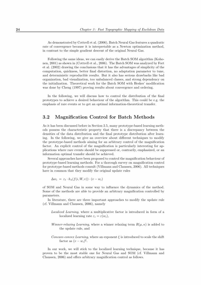
3.2 Magnification Control for Batch Methods
As it has been discussed before in Section 2.5, many prototype-based learning meth-ods possess the characteristic property that there is a discrepancy between thedensities of the data distribution and the final prototype distribution after learn-ing. In the following, we give an overview about different techniques to modifythe prototype-based methods aiming for an arbitrary control of the magnificationfactor. An explicit control of the magnification is particularly interesting for ap-plications where rare events should be suppressed or, contrarily, emphasized, or aninformation optimal transfer should be achieved.
Several approaches have been proposed to control the magnification behaviour ofprototype-based learning methods. For a thorough survey on magnification controlfor prototype-based methods consult (Villmann and Claussen, 2006). All techniqueshave in common that they modify the original update rules
Δwi = εt · hλ(f(i, W, v)) · (v − wi)
of SOM and Neural Gas in some way to influence the dynamics of the method.Some of the methods are able to provide an arbitrary magnification controlled byparameters.
In literature, there are three important approaches to modify the update rule(cf. Villmann and Claussen, 2006), namely
Localized Learning, where a multiplicative factor is introduced in form of alocalized learning rate εi = ε(wi),
Winner-relaxing Learning, where a winner relaxing term R(μ, κ) is added tothe update rule, and
Concave-convex Learning, where an exponent ξ is introduced to scale the shiftfactor as (v − wi)ξ.
In our work, we will stick to the localized learning technique, because it hasproven to be the most stable one for Neural Gas and SOM (cf. Villmann andClaussen, 2006) and offers arbitrary magnification control as follows.

3.2 Magnification Control for Batch Methods 25
Localized Learning in Neural Gas
Given a data distribution density function p, localized learning extends the learningrate in (2.9) by a factor which depends on the local data density:
Δwi = ε0 · p(ws(vj))c · hλ(ki(W, vj)) · (vj − wi) (3.6)
where ε0 > 0 is the learning rate and s(vj) is the winner index (2.3) for data pointvj . Parameter c controls the magnification exponent, where p(ws(vj))c vanishes forc = 0 leading to standard Neural Gas. That way, a local learning factor dependingon the data density at the winner location is added.
As shown by Villmann (2000), Neural Gas with the modified learning rule (3.6)asymptotically obeys the power law
�(wi) ∼ p(wi)α′with α′ = (c + 1) · α = (c + 1) · d
d + 2, (3.7)
where d is the intrinsic dimension of the data. Obviously, an information theoret-ically optimum factor α = 1 is obtained for c = 2/d. Larger values of c emphasizeinput regions with high data density, whereas smaller values put a focus on regionswith rarely sampled data points.
A drawback of the above approach is the need to calculate the density p(ws(vj))at the winning prototype location in each step. Having a transfer of magnificationcontrol to batch variants in mind, it would come in handy to precalculate datadensities at the locations of the data points of the finite dataset and rely only onthese values. With this motivation in mind, we consider the similar learning rule
Δwi = ε0 · p(vj)c · hλ(ki(W, vj))(vj − wi) , (3.8)
where the local density at the location of the sampled data point is taken insteadof that at the location of the winning prototype.
Now, the average of the learning rule (3.8) can be formulated as an integral
〈Δwi〉 ∼∫
p(v)c · hλ(ki(W, v)) · (v − wi) · p(v) dv. (3.9)
Since the magnification factor of localized learning has been derived under theassumption of a continuum of prototypes, where ws(v) = v holds, the average update(3.9) yields exactly the same result as the original one (3.6) proposed by Villmann(2000). Thus, the same magnification factor (3.7) results also for the altered learn-ing rule (3.8).
Moreover, the alternative update (3.8) has the benefit that it performs a stochas-tic gradient descent on the cost function
Eλ(W, c) =1
2C(λ)
n∑i=1
∫V
hλ(ki(W, v)) · ‖wi − v‖2 · p(v)c+1 dv. (3.10)
That is because (cf. Hammer et al., 2007b) the derivative of cost function (3.10)is given by
∂Eλ(W, c)∂wl
=1
C(λ)
∫V
hλ(ki(W, v)) · (wl − v) · p(v)c+1 dv
+1
2C(λ)
n∑i=1
∫V
h′λ(ki(W, v)) · ∂ki(W, v)
∂wl· ‖wi − v‖2 · p(v)c+1dv .

26 Chapter 3 : Fast Topographic Mapping of Euclidean Data
It has been shown in (Hammer et al., 2007b) that the second term vanishes.The first term complies straightforward with the average update rule (3.9). Hence,a stochastic gradient descent on the cost function (3.10) is performed when usingupdate rule (3.8).
Thus, learning schemes which optimize the cost function Eλ(W, c) yield a mapformation with magnification factor α′ as given by Eq. (3.7).
Note that for an application of the learning rule (3.6), the density p of the datadistribution as well as the effective data dimensionality d have to be estimatedfrom the data. These estimations can be done by standard techniques, e.g. Parzenwindow estimators, and the algorithm of Grassberger and Procaccia (1983), but ingeneral those are indeed difficult problems that are widely discussed in literature(Scott, 1992; Tong, 1993).
Transfer of Localized Learning to Batch Neural Gas
The formulation of localized learning by the modified update rule (3.8) that onlyrelies on local densities at data locations opens a way to integrate magnificationcontrol into Batch Neural Gas as follows.
For a given finite dataset V = {v1, v2, . . . , vm} the cost function (3.10) becomes
Eλ(W, c) =1
2C(λ)
n∑i=1
m∑j=1
hλ(ki(W, vj)) · ‖wi − vj‖2 · p(vj)c. (3.11)
As beforehand in (3.2), we substitute the terms ki(W, vj) by hidden variables kij ,where {kij : i ∈ {1, 2, . . . , n}} is a permutation of {0, 1, . . . , n − 1} for every j ∈{1, 2, . . . , m}. This yields
Eλ(W, c, kij) =1
2C(λ)
n∑i=1
m∑j=1
hλ(kij) · ‖wi − vj‖2 · p(vj)c . (3.12)
Batch optimization in turn determines optimum kij , given prototype locations, andoptimum prototype locations, given values kij . With the same arguments as usedbefore (cf. page 20), the optimal assignments kij are given by the ranks for fixedprototype locations W .
It can be seen further by setting the partial derivatives of Eq. (3.12) to zero,
∂Eλ(W, c, kij)∂wi
=1
C(λ)
m∑j=1
hλ(kij)(wi − vj) · p(vj)c != 0 ,
that the optimum prototypes wi for fixed assignments kij are given by the averageof the points weighted by the ranks and local data densities,
wi =
∑j hλ(kij) · p(vj)c · vj∑
j hλ(kij) · p(vj)c. (3.13)
The optimality follows in analogy to the discussion in the context of Batch NeuralGas (cf. page 22).
Hence, we obtain a Batch Neural Gas algorithm with local learning featuring amagnification exponent of (c+1) · d/(d+2) that provides an arbitrary control of themagnification via control parameter c. As discussed beforehand, the intrinsic datadimensionality d and the local data density p(vj) at the positions of the data points
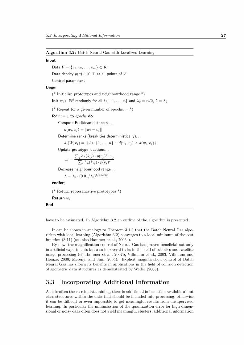
3.3 Incorporating Additional Information 27
Algorithm 3.2: Batch Neural Gas with Localized Learning
Input
Data V = {v1, v2, . . . , vm} ⊂ �d
Data density p(v) ∈ [0, 1] at all points of V
Control parameter c
Begin
(* Initialize prototypes and neighbourhood range *)
Init wi ∈ �d randomly for all i ∈ {1, . . . , n} and λ0 = n/2, λ = λ0
(* Repeat for a given number of epochs. . . *)
for t := 1 to epochs do
Compute Euclidean distances. . .
d(wi, vj) = ‖wi − vj‖Determine ranks (break ties deterministically). . .
ki(W, vj) = |{ l ∈ {1, . . . , n} : d(wl, vj) < d(wi, vj)}|Update prototype locations. . .
wi =
∑j hλ(kij) · p(vj)c · vj∑
j hλ(kij) · p(vj)c
Decrease neighbourhood range. . .
λ = λ0 · (0.01/λ0)t/epochs
endfor;
(* Return representative prototypes *)
Return wi
End.
have to be estimated. In Algorithm 3.2 an outline of the algorithm is presented.
It can be shown in analogy to Theorem 3.1.3 that the Batch Neural Gas algo-rithm with local learning (Algorithm 3.2) converges to a local minimum of the costfunction (3.11) (see also Hammer et al., 2006c).
By now, the magnification control of Neural Gas has proven beneficial not onlyin artificial experiments but also in several tasks in the field of robotics and satelliteimage processing (cf. Hammer et al., 2007b; Villmann et al., 2003; Villmann andHeinze, 2000; Merenyi and Jain, 2004). Explicit magnification control of BatchNeural Gas has shown its benefits in applications in the field of collision detectionof geometric data structures as demonstrated by Weller (2008).
3.3 Incorporating Additional Information
As it is often the case in data mining, there is additional information available aboutclass structures within the data that should be included into processing, otherwiseit can be difficult or even impossible to get meaningful results from unsupervisedlearning. In particular the minimization of the quantization error for high dimen-sional or noisy data often does not yield meaningful clusters, additional information
28 Chapter 3 : Fast Topographic Mapping of Euclidean Data
such as cluster labels or correlation can help to improve the quality. This issue isalso named ‘garbage in - garbage out’ problem of unsupervised learning and is dis-cussed e.g. by Kaski et al. (2005, 2003).
For an integration of additional information into prototype-based methods, wepresume that the additional information is available in form of a class label for eachdata point (cf. Villmann et al., 2006). Without loss of generality, we assume thatthese data labels are embedded in �c by an unary encoding of the c classes. Letthe label that is attached to a data point vj ∈ V be denoted by vL
j ∈ �c, i.e. vLj is
a vector with component (vLj )(k) = 1 iff vL
j represents class k, and (vLj )(k) = 0 else.
Additionally, each prototype wi features a label wLi ∈ [0, 1]c which shall be
adapted during learning depending on the label distribution of the data points inits neighbourhood. By the above construction, we are able to interpret the proto-type labels wL
i as a collection WL =(wL
i
)i∈{1,...,n} of prototypes in the label space
L = [0, 1]c.
To integrate supervision into a prototype-based method, we now substitute theoriginal Euclidean metric in the cost function Eλ(W ) by a combination of the metricin data space and the metric in label space, yielding a new cost function
E∗λ(W, WL, β) =
12
n∑i=1
m∑j=1
hλ(ki(W, vj))·((1 − β) · ‖wi − vj‖2 + β · ∥∥wL
i − vLj
∥∥2)
,
where the weighting of the metric in data space and the metric in label space iscontrolled by parameter β.
In this section, we have chosen Batch Neural Gas as a representative example.Nevertheless the concept can easily be migrated to other prototype-based batchmethods like Batch SOM (Hammer et al., 2006b).
Alternating optimization as introduced beforehand leads to new update rulesfor the prototypes W in data space and the prototypes WL in label space. It caneasily be seen that the cost function separates such that the update rule for theprototypes in data space stays the same as before Eq. (3.5), and the prototypelabels are updated in label space by the same rule, i.e. we have
wLi =
∑j hλ(kij) · vL
j∑j hλ(kij)
for all i ∈ {1, 2, . . . , n}. (3.14)
The optimal assignments kij are determined subject to a modified rank functionthat is based on the combined metric. That way, the additional label informationexerts influence on the prototype updates in data space turning the unsupervisedmethods into a supervised one.
It follows directly from the update rule that the components of each prototypelabel sum up to 1 and are therefore interpretable as probabilities or fuzzy labels.Crisp labels can be obtained by applying e.g. the majority vote principle.
There is another way to interpret the chosen approach of supervision in the Eu-clidean setting. It can easily be seen that if the data space is Euclidean, data spaceand label space can be embedded into �d+c by vectors (
√1 − β · x,
√β · xL). The
squared Euclidean norm then results in ‖(√1 − β · x,√
β · xL)‖2 = (1 − β) · ‖x‖2 +β · ∥∥vL
∥∥2, which yields the same separable cost function as above. Thus, applyingthe standard batch methods on the embedded Euclidean vector set is equivalent tothe supervised batch methods introduced above.

3.3 Incorporating Additional Information 29
All the batch variants of Neural Gas, SOM, and kMeans can be modified likepresented above to incorporate additional label information. The convergence of thesupervised variants is guaranteed for all the methods as shown in (Hammer et al.,2006b). In Algorithm 3.3 a sketch of the Supervised Batch Neural Gas algorithm(Hammer, Hasenfuss, Schleif, and Villmann, 2006b) is shown as a representativeexample.
Algorithm 3.3: Supervised Batch Neural Gas
Input
Data V = {v1, v2, . . . , vm} ⊂ �d
Labels{vL1 , vL
2 , . . . , vLm
} ⊂ �c
Begin
(* Initialize prototypes and neighbourhood range *)
Init wi ∈ �d randomly for all i ∈ {1, . . . , n} and λ0 = n/2, λ = λ0
(* Repeat for a given number of epochs. . . *)
for t := 1 to epochs do
Compute distances. . .
d∗β(wi, vj) = (1 − β) · ‖wi − vj‖2 + β∥∥wL
i − vLj
∥∥2
Determine ranks (break ties deterministically). . .
ki(W, vj) =∣∣∣{ l ∈ {1, . . . , n} : d∗β(wl, vj) < d∗β(wi, vj)
}∣∣∣Update prototype locations. . .
wi =∑
j hλ(kij) · vj/∑
j hλ(kij)
Update prototype labels. . .
wLi =
∑j hλ(kij) · vL
j /∑
j hλ(kij)
Decrease neighbourhood range. . .
λ = λ0 · (0.01/λ0)t/epochs
endfor;
(* Return representative prototypes and prototype labels *)
Return wi and wLi
End.
The introduced modification now allows to incorporate additional informationinto the learning process which turns the original unsupervised methods into su-pervised ones. This supervision helps to improve the quality of the results becausethe receptive fields are influenced by the underlying class information. Especially,when the prototypes are used as a classifier, this leads to a better generalizationability as it can be seen from the experiments in Section 3.5.
Up to now, we have been discussing methods that are capable of dealing withten thousands of datapoints from Euclidean spaces. But nowadays there are manysituations where the practitioner is facing datasets with millions of points. Whilehandling those huge datasets, the computational limits of the standard methods,

30 Chapter 3 : Fast Topographic Mapping of Euclidean Data
even those of the fast batch approaches, quickly arise. In the following, we willpresent a technique to handle even those very large datasets by prototype-basedmethods. The introduced technique is based on patches of smaller size that areconsecutively cut from the dataset. While processing the patches, statistical infor-mation gained from the processing of former patches is taken into account.
3.4 Processing of Very Large Datasets
Twenty month from now, the amount of electronic data stored worldwide will bedoubled—and the rate is accelerating. In many fields, e.g. computational biology,image processing, or particle physics, vast amounts of data are produced from dayto day in experiments. As a consequence, nowadays almost every scientific disci-pline is facing the problem to handle huge data repositories. Here, automatic datamining constitutes an indispensable tool bridging the gap between available dataand desired knowledge which would otherwise be inaccessible. Some of the bigchallenges of real-world data mining have been identified in a panel discussion atthe 2007 SIAM International Conference on Data Mining as follows (Hirsh, 2008):Mining massive data which go beyond the capacities of standard algorithms, min-ing streaming data which is generated in a continuous process and which requiresimmediate feedback, mining heterogeneous data which stem from different sources,applicability of methods and interpretability of the results by researchers outsidethe data mining community, among others. These facts pose particular require-ments towards standard data mining tools concerning their efficiency, flexibility,and interpretability.
Prototype-based techniques, like the above introduced SOM and Neural Gas,possess several striking features because of which they are widely used in appli-cations: training is intuitive and simple, the final classifier represents classes bygeometrically meaningful prototypes, and the algorithms are quite powerful com-pared to more complex alternative clustering algorithms.
The original online variants that sample point for point from the dataset canbe applied to very large datasets without restrictions but due to their convergenceproperties (Martinetz et al., 1993; Kohonen, 2001) the computation time neededmight be beyond practical limits.
In the fast batch variants, all data is used for every iteration over and overagain. But for a reasonable performance it is necessary to hold all data at oncein random-access memory during computation. Unfortunately, those very largedatasets cannot be held at once within memory for processing due to the sheeramount of data.
To fill the gap, a special computation scheme is introduced, relying on a singlepass technique of fixed sized patches. In between processing of the patches a suffi-cient statistic is passed over describing the data distribution in the former patches.The patch size can then be chosen to match the given memory constraints. Theproposed patch versions reduce the computation and space complexity with a smallloss of accuracy. As beforehand, we develop the idea on the basis of Neural Gas togive a concrete and clear representation, how to migrate the idea to SOM or otherprototype-based methods is obvious besides technicalities.
A variant of Neural Gas for very large datasets was introduced by Alex et al.(2009). It is based on a patch processing scheme that splits the dataset into anumber of disjunct patches and applies Batch Neural Gas consecutively on eachpatch. Additionally, each patch is enhanced by the prototypes of the processing ofthe former patch weighted by the sizes of their receptive fields. That way, a suffi-cient statistic of former data is transferred in between the patches. Batch Neural
3.4 Processing of Very Large Datasets 31
Gas in conjunction with this patch scheme shows a very good performance in theexperiments. Moreover, it can easily be parallelized with an almost linear speedupas shown in (Alex and Hammer, 2008). Open questions by now concern with theexistence of bounds on the quantization error and the sufficiency of the statisticsfrom a theoretical point of view.
In the following, the Patch Neural Gas algorithm is presented in more detail, lay-ing the foundations to build on in later chapters about patch schemes for prototype-based methods in non-Euclidean spaces.
Patch Neural Gas
Assume a finite dataset V = {v1, v2, . . . , vm} ⊂ �d is given. During processing ofPatch Neural Gas, np disjoint patches of fixed size p = �m/np� are taken from thedataset V consecutively1, i.e. every patch Pi is a subset of V and it holds
⋃i Pi = V .
The idea of the patch scheme is to add the set of final prototypes Wt−1 fromthe processing of the former patch Pt−1 as additional weighted datapoints to thecurrent patch Pt, forming an extended patch P ∗
t = Pt ∪ Wt−1 to work on further.Every original datapoint vj ∈ V is equipped with a multiplicity m(vj) = 1.
The additional datapoints – as former prototypes – are weighted according to thesize of their receptive fields taking into account possible multiplicities, i.e. howmany datapoints they have been representing in the former patch counted withmultiplicities. The multiplicity m(wi) of a prototype wi ∈ Wt is then given by
m(wi) =∑
v∈P∗t ∩Vi(Wt)
m(v).
Now, the original Batch Neural Gas method must be modified to take intoaccount the multiplicities. Incorporating the multiplicities into the cost function(3.2) yields
Eλ(W, kij) =12
∑i
∑j
hλ(kij) · m(vj) · ‖wi − vj‖2,
since every datapoint vj is weighted with multiplicity mj. The new update rule forthe prototypes derived from the modified cost function in analogy to (3.5) is givenby
wi =
∑j hλ(kij) · m(vj) · vj∑
j hλ(kij) · m(vj)for all i ∈ {1, 2, . . . , n}.
For the processing of each patch, all properties concerning optimal assignments andconvergence follow the same way as in Section 3.1, since the multiplicities can beinterpreted as multiples of a single point.
Picking up the pieces, we obtain the Patch Neural Gas algorithm (Alex, Hasenfuss,and Hammer, 2009) as sketched in Algorithm 3.4.
Using the above introduced technique of patch processing, it is now possible tohandle very large datasets with millions of data points. The technique has shownits strength in several experiments as it can be seen in Section 3.5 and also later onin Section 4.6.
In the next section, we will present experimental results for all of the aboveintroduced methods and techniques.
1The remainder is no further considered here for simplicity. In the practical implementationthe remaining datapoints are simply distributed over the first (M − p · np) patches.

32 Chapter 3 : Fast Topographic Mapping of Euclidean Data
Algorithm 3.4: Patch Neural Gas
Begin
Cut the first Patch P1
Apply Batch Neural Gas on P1 −→ Prototypes W1
Update Multiplicities m(W1)
Repeat for i = 2, . . . , np
Cut patch Pi
Construct Extended Patch P ∗i = Pi ∪ Wi−1
Apply modified Batch Neural Gas with Multiplicities
−→ Prototypes Wi
Update Multiplicities m(Wi)
Return final Prototypes Wnp
End.
3.5 Experimental Results and Applications
In the following, experimental results and applications of the above introducedmethods are presented. The data in the assessment was chosen to cover differentaspects that are common in real-life applications, or to demonstrate the behaviourof the methods in situations which are of theoretical importance. Also, most ofthe times, data that has already been used in literature was chosen to provide acomparison to the state-of-the-art. There emerged already some interesting appli-cations of the methods, most notably Batch Neural Gas has proved its amenitiesin the efficient compression of sequences of 3D models in Computer Graphics bydetermining key-frames in a very fast way (Winkler et al., 2008).
Experimental Results on Batch Methods
We demonstrate the behavior of the algorithms in different scenarios which covercharacteristic situations. All algorithms have been implemented based on the SOMToolbox for Matlab (Vesanto et al., 2000). We used k-means, SOM, and OnlineNeural Gas with default parameters as provided in the toolbox. Batch NG andBatch SOM have been implemented according to the above formulas. Note, that thetraining sets are normalized prior to training using the z-transformation, i.e. datais normalized in a way that the expectation value in each dimension is 0 and thestandard deviation is 1. Initialization of prototypes takes place using small randomvalues. The initial neighborhood rate for neural gas is set to λ = n/2, n being thenumber of neurons, and it is multiplicatively decreased during training. For SOM,we used square lattices of n =
√n × √
n neurons and a rectangular neighborhoodstructure, whereby
√n is rounded to the next integer. Here the initial neighborhood
rate is√
n/2. To measure the quality of the mapping the empirical quantizationerror according to eq. (2.2) was determined.
Synthetic data
The first data set is the two-dimensional synthetic data set from (Ripley, 1996)consisting of 250 data points and 1000 training points. Clustering has been done

3.5 Experimental Results and Applications 33
using n = 2, . . . , 25 prototypes, resp. the closest number of prototypes implementedby a rectangular lattice for SOM. Training takes place for 5n epochs.
The mean quantization error on the test set is shown in Fig. 3.1. For k-means,idle prototypes can be observed for large n. For Batch SOM and standard SOM,the quantization error is worse (ranging from 1.7 for two neurons up to 0.3 for 24neurons, not depicted in the diagram), which can be attributed to the fact that themap does not fully unfold upon the data set and edge effects remain, which couldbe addressed to a small but non-vanishing neighborhood in the convergent phase instandard implementations of SOM which is necessary to preserve topological order.Thus, Batch NG allows to achieve results competitive to NG in this case, however,using less effort. The median variants whose results are also displayed in the figurewill be discussed later on.
Segmentation data
The segmentation data set from the UCI repository consists of 210 (training set)resp. 2100 (test set) 19 dimensional data points which are obtained as pixels fromoutdoor images preprocessed by standard filters such as averaging, saturation, in-tensity, etc. The problem is interesting since it contains high dimensional and onlysparsely covered data. The quantization error obtained for the test set is depictedin Fig. 3.1. As beforehand, SOM suffers from the restriction of the topology. Neu-ral gas yields very robust behavior, whereas for k-means, idle prototypes can beobserved.
Checkerboard
This data set is taken from (Hammer et al., 2005). Two-dimensional data arearranged on a checkerboard (cf. Figure 3.12), resulting in 10 times 10 clusters, eachconsisting of 15 to 20 points. For each algorithm, we train 5 times 100 epochsfor 100 prototypes. Obviously, the problem is highly multimodal and usually thealgorithms do not find all clusters. The number of missed clusters can easily bejudged in the following way: the clusters are labeled consecutively using labels 1and 2 according to the color black resp. white of the data on the correspondingfield of the checkerboard. We can assign labels to prototypes a posteriori based ona majority vote on the training set. The number of errors which arise from thisclassification on an independent test set count the number of missed clusters, since1% error roughly corresponds to one missed cluster.
Online Batch Online Batch BatchNG NG SOM SOM k-Means
quantization errortrain 0.0043 0.0028 0.0127 0.0126 0.0043test 0.0051 0.0033 0.0125 0.0124 0.0050classification errortrain 0.1032 0.0330 0.2744 0.2770 0.1136test 0.1207 0.0426 0.2944 0.2926 0.1376
Table 3.1: Quantization error and classification error on Checkerboard Data forposterior labeling for training and test set (both are of size about 1800). The meanover 5 runs is reported. The best results on the test set is depicted in boldface.
The results are collected in Tab. 3.1. The smallest quantization and classificationerror is obtained by Batch NG. As beforehand, SOM and Batch SOM do not fully

34 Chapter 3 : Fast Topographic Mapping of Euclidean Data
unfold the map in the data. In the same way online NG does not achieve a smallerror because of a restricted number of epochs and a large data set which preventsonline NG from fully exploring the data space. K-means also shows a quite higherror (it misses more than 10 clusters) which can be explained by the existence ofmultiple local optima in this setting, i.e. the sensitivity of k-means with respect toinitialization of prototypes. In contrast, Batch NG finds all but 3 to 4 clusters.Hence, batch versions show much better behavior than their online correspondents,due to a faster convergence of the algorithms. Here, SOM suffers from border effects,whereby the topology mirrors precisely the data topology. Batch NG yields quitegood classification results which are even competitive to supervised prototype-basedclassification results as reported in (Hammer et al., 2005).
Experimental Results on Supervised Methods
Artificial data
The main difference of Batch NG (BNG) with posterior labeling and SupervisedBatch NG (SBNG) consists in the fact that the rank assignments also take intoaccount whether the labels fit. This has the effect that the prototypes of SBNGbetter account for cluster borders of labeled data points, whereas BNG only followsthe overall statistics. The parameter β controls the strength of the label contribu-tion, β = 1 corresponds to the original BNG. This effect can be clearly observedin the following example. We consider two Gaussian clusters labeled by 0 resp. 1,whereby points with x-component at least 0 are dropped for class 0, and pointswith x-component at most 0 are dropped for class 1. Hence, the classes are wellseparated, whereby a couple of data points lies close to the decision boundary. Fig-ure 3.2 shows a typical result of the receptive fields of the prototypes obtained byBNG and SBNG with mixing parameter β = 0.1, respectively.
Thereby, prototypes of BNG are labeled by a majority vote within the receptivefield. Fuzzy labels for SBNG arise automatically during training, these are turnedinto crisp classes based on the largest component of the label vector. Obviously,SBNG well approximates the decision border, whereas BNG yields a couple of errorsat this region. This corresponds to the classification accuracy of 99.1% for SBNGand 97.8% for BNG.
Iris data
We train batch BNG and SBNG using 9 prototypes on the well-known iris dataset,which consists of 150 points characterized by 4 real-valued attributes coming fromthree classes of equal size. Class 1 is well separated from class 2 and 3, but classes2 and 3 slightly overlap. The task here is to train a classifier on a subset of thedata and assess the trained classifier with the remaining part. The accuracy, i.e.the fraction of correctly classified data points, is measured. For each run, the setis randomly divided into a training and test set of equal size, and averages of theaccuracy over 50 runs are reported. The neighborhood range λ is multiplicativelyannealed starting from 4.5 over 100 training epochs. Different values of the mixingparameter β are reported.
The classification accuracy on the training and test set for SBNG and, in com-parison, for BNG with posterior labeling can be observed in Fig.3.3. Obviously,the classification accuracy becomes better for smaller β, i.e. more emphasis of thegiven data labels. Thereby β must not become 0 which corresponds to a pure labeladaptation without adaptation of the prototypes. β = 1 corresponds to the originalBNG. The classification accuracy of the original BNG is inferior compared to thesupervised version due to the overlap of classes 2 and 3 which is not accounted for

3.5 Experimental Results and Applications 35
by the overall statistics of the input vectors. The algorithm reported in (Villmannet al., 2006) (Gaussian approximation) achieves (in a single run with parameterβ = 0.5) a training set accuracy of 0.85 and test set accuracy of 0.91 using 9 pro-totypes, thus it is better than post labeled NG, but worse compared to SupervisedBatch NG for this parameter choice.
Wisconsin breast cancer
The well-known Wisconsin breast cancer data (WDBC) consists of 569 data pointsdescribed by 30 real-valued input features. It originates from medical researchwhere fine needle aspiration biopsy was applied to suspicious breast masses andmicroscope images of the tissues were analyzed. Ten real-valued features describingcharacteristics of cell nuclei like radius, perimeter, fractal dimension, symmetry,concavity, etc. were gathered. For every of the ten features the mean, standarddeviation, and the largest value over all observed cells were calculated leading to30-dimensional data points. The task is to determine whether the sample is benignor malignant. There are 357 benign and 212 malignant samples.
For training 20 prototypes were used and the same parameters as beforehand,starting with an initial neighborhood range 10. The results are presented in Fig.3.4.As before, a larger emphasis on the correctness of the labels yields a better classi-fication accuracy which is superior to BNG. Interestingly, the approach presentedin (Villmann et al., 2006) which relies on a different supervised extension of NG(Gaussian approximation of the rank) achieves an accuracy of 0.92 for the trainingset and 0.91 on the test set for a mixing parameter 0.5, which is in this case worsethan the result obtained by BNG with posterior labeling.
Experimental Results on Magnification Control
For all experiments the initial neighborhood range λ0 is chosen as n/2 with n thenumber of neurons used. The neighborhood range λ(t) is decreasing exponentiallywith the number of adaptation steps t according to λ(t) = λ0 · (0.01/λ0)t/tmax (cf.Martinetz et al., 1993). The value tmax is given by the number of epochs of atraining run.
Control experiment
In a first control experiment we use the setting as proposed e.g. in (Villmann andClaussen, 2006). We use the distribution (x1, . . . , xd,
∏di=1 sin(π·xi)) for d ∈ {1, 2, 3}
and uniformly distributed xi in [0, 1]. Thus, the intrinsic data dimensionality inthese examples is d = d. The number of stimuli is 2500 for d = 1, 5000 for d = 2,and 10000 for d = 3. These numbers account for the fact that the necessary numberof data points to sufficiently sample a d-dimensional data space grows exponentiallywith d. Due to computational complexity a k · 2d - scheme with a large constantk = 2500 was chosen instead of kd.
Optimum information transfer for NG with magnification control can be ex-pected for values which yield α′ = (c + 1) · d/(d + 2) != 1, where c is the controlparameter and d the intrinsic dimensionality of data. Hence, it is c = 2 (d = 1),c = 1 (d = 2), and c = 2/3 (d = 3). We train an NG network with magnificationcontrol for control values c ∈ [−1.5, 3.5] (step size 0.25) such that the overall be-havior of the local learning rule for different c can be observed. An NG networkwith 50 neurons, initial neighborhood range 25 and 200 epochs per training run hasbeen used. The reported results have been averaged over 20 runs. The data densityp(v) has been estimated by a Parzen window estimator with bandwidth given bythe average training point distances divided by 3.

36 Chapter 3 : Fast Topographic Mapping of Euclidean Data
The information theoretic quality of the information transfer of the map can bejudged by counting the balance of patterns in the receptive fields. For equal values,optimum information transfer is achieved. We count the number of data points ofthe training set in the receptive of a given prototype averaged over the number ofdata points and report the entropy thereof. The resulting values are reported inFig. 3.5. The entropy should be maximum for optimum information transfer, i.e.we expect the optimum for c = 2 (d = 1), c = 1 (d = 2), and c = 2/3 (d = 3),respectively. As indicated by the arrows, the experimental optimum of the curves isvery close to the expected theoretical values in all cases, thus confirming the theorypresented in this thesis.
Remote sensing image analysis
In geophysics, geology, astronomy, and many environmental applications airborneand satellite-borne remote sensing spectral imaging has become one of the mostadvanced tools for collecting vital information about the surface of the Earth andother planets. Thereby, automatic classification of intricate spectral signatures hasturned out far from trivial: discrimination among many surface cover classes anddiscovery of spatially small, interesting species proved to be an insurmountable chal-lenge to many traditional methods. Usually, spectral images consist of millions ofdata points such that clustering often becomes a necessary prerequisite for furtherprocessing and inspection. Thereby, it is often crucial to preserve characteristicsfrom spatially small interesting regions which are easily oppressed by standard vec-tor quantization. Here we show that magnification control can help to preserve thecharacteristics of rare classes.
We consider a LANDSAT TM image from the Colorado area, U.S.A., for whicha manually generated label map of surface covers is available. The original imagecovers an area of about 50x50 kilometers yielding approximately 2 million datapoints which can be divided into 14 classes with different surface covers. Dataare 6-dimensional, the thermal band with low resolution was left away. An initialGrassberger-Procaccia analysis yields the intrinsic dimensionality d = 3.1414 (Vill-mann et al., 2003). For the experiments, we randomly selected 17004 data pointswith a representative class distribution. Tab. 3.2 shows the different surface covertypes and their respective percentage. As depicted in Tab. 3.3 dimensions 1, 2, 3,5, and 6 are correlated.2
Therefore, we depict the projection onto dimensions 1 and 4. Data are approx-imately unimodal with several small characteristics at the data borders, as can beseen in Fig. 3.9. The second largest class (1-scotch pine) lies very close to the centerof gravity, the largest one (13-dry meadow) a bit off center. Small extremal classesat the data borders are given by 9-water and 14-alpine vegetation.
We train a neural map with 60 neurons for 100 epochs. The local data densityis estimated by Parzen windows as before. Thereby, we use different control values.The final location of neurons is depicted in Figs. 3.6-3.8 for α = 0.01, α = 0.61 (i.e.standard neural gas), and α = 2. Thereby, the star denotes the center of gravityof the data points. Obviously, the neurons focus on the common effects and movetowards the center of gravity for large values of α, whereas they sample rare effectsat the borders (e.g. class 14 at the upper right corner) for small values of α.
This behavior can be quantified by counting the number of neurons responsiblefor a given class. Thereby, neurons are labeled according to a majority vote ontheir receptive field. The number of hits for every class averaged over 10 runs isdepicted in Fig. 3.10. c = 0 corresponds to standard NG, c = 0.64 is close to the
2This observation is also stressed when training a SOM using the data: the gradients of thecomponent planes of dimensions 1, 2, 3, 5, and 6 look very similar, whereas the gradient of thecomponent plane for dimension 4 is perpendicular.

3.5 Experimental Results and Applications 37
class number percentage surface cover type1 17.30% scotch pine2 10.46% Douglas fir3 5.32% pine/fir4 7.93% mixed pine forest5 4.26% supple/prickle pine6 6.13% aspen/mixed pine forest7 5.05% without vegetation8 8.12% aspen9 0.48% water10 2.83% moist meadow11 3.78% bush land12 7.78% grass/pastureland13 19.77% dry meadow14 0.79% alpine vegetation
Table 3.2: Surface cover classes and their respective percentage
dim 1 2 3 4 5 61 1 0.9564 0.9493 0.4691 0.8162 0.85442 0.9564 1 0.9678 0.5858 0.8448 0.86823 0.9493 0.9678 1 0.4867 0.8339 0.88974 0.4691 0.5858 0.4867 1 0.5783 0.44175 0.8162 0.8448 0.8339 0.5783 1 0.95746 0.8544 0.8682 0.8897 0.4417 0.9574 1
Table 3.3: Correlation coefficients of the data dimensions: Correlated dimensions1, 2, 3, 5, and 6 are shown in bold face.
information theoretic optimum. c → 0 focuses on rare events, whereas large valuesc account for final prototype locations in typical regions, the center of gravity asthe limit. The depicted values are c ∈ {−0.9836,−0.91817,−0.59, 0, 0.64, 2.27, 3.9}which corresponds to a magnification factor α ∈ {0.01, 0.05, 0.25, 0.61, 1.0, 2.0, 3.0}assuming d ≈ 3.1414. One can see that small classes at the borders of the data set(classes 9-water and 14-alpine vegetation) are represented by neurons only for smallvalues c which emphasize rare events. In the limit of large c, class 1 (scotch pine),which is the second largest class and located near the center of gravity, accumulatesmost neurons. Thus, magnification control allows, depending on the control values,to detect rare cover types or, conversely, to focus on the most representative surfacecover type in inspections.
Experimental Results on Patch Processing
We test patch and batch versions of k-means and NG for three different data sets, avery simple four-mode clustering problem, a highly-multimodal benchmark datasetfrom (Cottrell et al., 2006), and a large data set from the 1998 KDD cup data miningcontest which was also tested in (Farnstrom et al., 2000). For all experiments, clustercenters are initialized at random positions close to the origin which, due to datanormalization, constitutes a reasonable center point for all data sets. It can beobserved that the exact position of the initial prototypes has hardly an influence onthe overall results and virtually no influence if averaged over several runs, as done

38 Chapter 3 : Fast Topographic Mapping of Euclidean Data
Batch Patch Batch PatchKM KM NG NG
Mean quantization error (Four Clouds)1.25 1.28 1.25 1.26
Variance ·103
0.07 0.37 0.07 0.1
Mean classification accuracy in % (Checkerboard)patch size 200
87.32 86.38 93.35 90.18patch size 400
85.43 90.76patch size 600
84.47 91.80
Mean quantization error (KDD)patch size 1000
0.468 0.464 0.460 0.462variance ·103
0.265 0.265 0.03 0.012patch size 10000
0.468 0.461variance ·103
0.114 0.011
Table 3.4: Quantization error or classification accuracy, respectively, as obtained bythe different clustering algorithms for the Four Clouds data set, the Checkerboarddata set, and the KDD data set for batch and patch clustering using different patchsizes
in the experiments.
Four Clouds
Data stem from a mixture of four Gaussians with unit variance in two dimensionsas depicted in Fig. 3.11. The set consists of 40000 data points. Training is doneby ten-fold crossvalidation using four clusters and a random (i.i.d.) order of thepoints. Thereby, the results on the training and test sets differ only slightly. Weuse a crossvalidation to evaluate the robustness and sensitivity of the algorithm withrespect to noise. The patch size is 100, and each clustering of a patch includes 20epochs, thereby annealing the neighbourhood of NG from n/2 = 2 to 0. The meanvalue of the quantization error is given in Tab. 3.4. Obviously, the results are almostidentical for all runs due to the simplicity of the data set. Very slight differences ofthe quantization error are due to the fact that the points at the (overlapping) clusterborders are assigned differently. For all methods, the four cluster centers have beenfound in every run, showing no differences between batch- and patch-clustering anddifferent patch sizes, respectively, in the principled location of the cluster centers.
Checkerboard
Data constitute a multimodal distribution with 100 clusters in two dimensions asdepicted in Fig. 3.12 separated into a training and test set. The overall number ofdata points in both, training and test set is about 2000. Training is done using 100neurons. The patch size is chosen as 200, 400, and 600, respectively. The initialneighbourhood size of NG, 10, is annealed to 0 during training. The number ofepochs is 20 for each patch clustering. It is easily possible to evaluate the numberof missed clusters in this task by referring to the classification error of the under-lying checkerboard: we assign the label 0 and 1 to the data points such that a

3.5 Experimental Results and Applications 39
checkerboard-pattern with 100 fields arises. We label the cluster centers based onthe training set and evaluate the classification error of this clustering on the testset. Each percentage of misclassification corresponds to one missed cluster (of 100total clusters). The mean correct classification (in percentage) obtained in ten runsis reported in Tab. 3.4. In this case, the quantization error does not allow to inferthe quality of the clustering due to the large number of comparably small clusters:it is around 0.055 for batch and patch variants of k-means and NG, hardly showingany difference between batch and patch clustering.
The clustering results clearly show the following: the task is quite hard andall methods miss a few cluster centers (ranging from 15 for k-means to 7 for NG).Note that each of the 100 clusters is only represented, on average, by 20 datapoints, and the number of neurons is chosen exactly as 100, i.e. every neuron mustrepresent exactly one center for optimum classification accuracy. In these cases,a clear difference of patch and batch clustering can be observed: overall, patchclustering finds about 3-4 clusters less compared to batch clustering. This effectdepends slightly on the size of the patches, as can be observed in particular for NG.However, for reasonable patch size the loss in accuracy is only minor and it couldeasily be accounted for by using a slightly larger number of cluster centers thannecessary. In this scenario the dependency of k-means on initialization pops out forboth, batch and patch clustering.
Due to the intuitive evaluation of the clustering result by means of the classi-fication error, a comparison to online-neural gas, which can directly be applied tolarge data sets since it adapts the prototypes directly after every pattern, is easilypossible in this scenario: After only one pass through the data, no convergence canbe observed in the sense that the neurons are not located in the cluster centers atall. After about 5 epochs, convergence can be observed. On average, 15 clustersare missed after 5 epochs, about 10 clusters are missed after 10 epochs, about 8clusters are missed after 20 epochs (this setting is comparable to the setting testedfor batch NG, whereby batch NG obtains, on average, slightly better performance),about 5 clusters after 50 epochs, and about 3 after 100 epochs. Thus, several passesover the entire data set are necessary for online NG to show competitive results topatch NG.
KDD Cup Data Mining Contest
This data set stems from the 1998 KDD cup data mining contest, and we usethe same setting as proposed in (Farnstrom et al., 2000). Data contains 95412records with 481 statistical fields which describe statistical information about peoplewho made charitable donations in response to direct mailing requests. For ourexperiments, 56 features from these fields have been selected, including numericalfeatures such as donation amount, income, age; date values, such as donation date,date of birth; and binary values such as income category. Data are preprocessed suchthat only numerical values with zero mean and unit variance result. The number ofclusters was set to 10, as proposed in (Farnstrom et al., 2000), and the number ofepochs is 20. The mean quantization error averaged in a ten-fold crossvalidation isreported in Tab. 3.4 for two different patch sizes corresponding to roughly 1% and10% of the data, respectively. Since the preprocessing in (Farnstrom et al., 2000)has been described only qualitatively, we cannot compare to the results reportedthere, but we test k-means in our setting. Obviously, a slight improvement of NGcompared to k-means can be observed, whereby patch clustering using 10% of thedata only slightly reduces the achieved results. Interestingly, the variance of theresults can be reduced by patch clustering compared to batch clustering, and – asexpected – NG compared to k-means. However, it is clearly demonstrated that forall variants, patch optimization only slightly decreases the overall result whereby
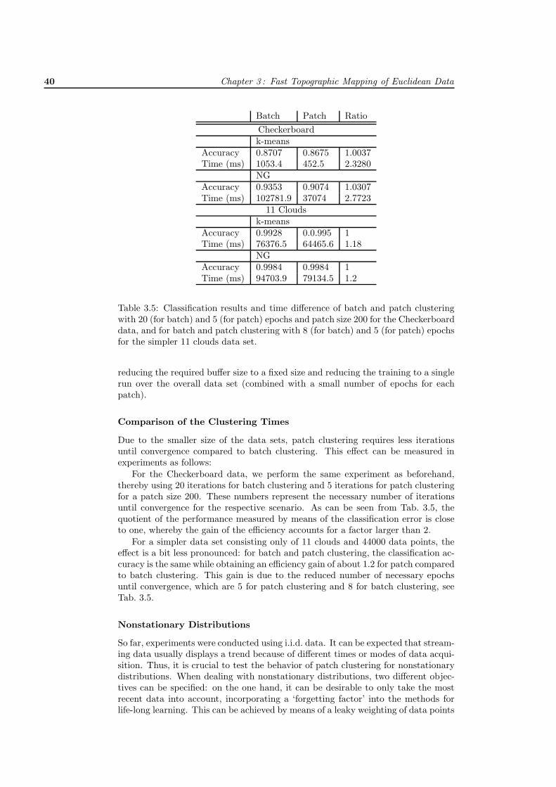
40 Chapter 3 : Fast Topographic Mapping of Euclidean Data
Batch Patch RatioCheckerboardk-means
Accuracy 0.8707 0.8675 1.0037Time (ms) 1053.4 452.5 2.3280
NGAccuracy 0.9353 0.9074 1.0307Time (ms) 102781.9 37074 2.7723
11 Cloudsk-means
Accuracy 0.9928 0.0.995 1Time (ms) 76376.5 64465.6 1.18
NGAccuracy 0.9984 0.9984 1Time (ms) 94703.9 79134.5 1.2
Table 3.5: Classification results and time difference of batch and patch clusteringwith 20 (for batch) and 5 (for patch) epochs and patch size 200 for the Checkerboarddata, and for batch and patch clustering with 8 (for batch) and 5 (for patch) epochsfor the simpler 11 clouds data set.
reducing the required buffer size to a fixed size and reducing the training to a singlerun over the overall data set (combined with a small number of epochs for eachpatch).
Comparison of the Clustering Times
Due to the smaller size of the data sets, patch clustering requires less iterationsuntil convergence compared to batch clustering. This effect can be measured inexperiments as follows:
For the Checkerboard data, we perform the same experiment as beforehand,thereby using 20 iterations for batch clustering and 5 iterations for patch clusteringfor a patch size 200. These numbers represent the necessary number of iterationsuntil convergence for the respective scenario. As can be seen from Tab. 3.5, thequotient of the performance measured by means of the classification error is closeto one, whereby the gain of the efficiency accounts for a factor larger than 2.
For a simpler data set consisting only of 11 clouds and 44000 data points, theeffect is a bit less pronounced: for batch and patch clustering, the classification ac-curacy is the same while obtaining an efficiency gain of about 1.2 for patch comparedto batch clustering. This gain is due to the reduced number of necessary epochsuntil convergence, which are 5 for patch clustering and 8 for batch clustering, seeTab. 3.5.
Nonstationary Distributions
So far, experiments were conducted using i.i.d. data. It can be expected that stream-ing data usually displays a trend because of different times or modes of data acqui-sition. Thus, it is crucial to test the behavior of patch clustering for nonstationarydistributions. When dealing with nonstationary distributions, two different objec-tives can be specified: on the one hand, it can be desirable to only take the mostrecent data into account, incorporating a ‘forgetting factor’ into the methods forlife-long learning. This can be achieved by means of a leaky weighting of data points

3.5 Experimental Results and Applications 41
or prototypes, respectively, for patch clustering. However, we are not interested inthe scenario of life-long learning in this contribution. Rather, we are interested inthe question whether patch clustering can achieve results competitive to full batchclustering also if the consecutive patches are non i.i.d. but display a trend. Thus thequestion is whether the representation of already seen data points by means of pro-totype centers is sufficient even if the prototypes are not yet remotely representativefor the full data set.
We test this question by means of the 11 clouds distribution as beforehand, seeFig. 3.13. We use a data set consisting of 11000 points. The patch size is 1000, i.e. itcorresponds to one mode of the data. We present the data set in three different waysto patch clustering, for comparison: randomly permuted i.i.d. data, data which arestrictly sorted according to the modes (from left to right and bottom to top), anddata which are mixed in such a way that every patch comprises 56% of a specifiedmode and 21% resp. 1% of the immediate two preceding and succeeding modes. Wetrain patch clustering using 100 epochs per patch. The exact data presentation forevery patch as well as the results of patch clustering after every patch are displayedin Figs. 3.14,3.15,3.16. As can be seen, the behavior is very robust with respect tothe final results: in all runs, the final clustering is almost identical with respect tothe given data distribution. Interestingly, the third case, where modes are presentedconsecutively subject to a diffusion process, seems the most difficult setting in thiscase. The clustering is affected by this distribution in the form of a small shift of theideal center of cluster 7 to the right in the final result as can be seen in Fig.3.16 inthe last three patches. However, the receptive fields in the data set are not affectedby this small shift.
As it can be seen from the experiments, the batch variants of the prototype-basedmethods generate results of the same quality as the standard online approaches butmuch faster. Also the extensions to supervision, magnification control, and patchprocessing have shown their benefits in the experiments.
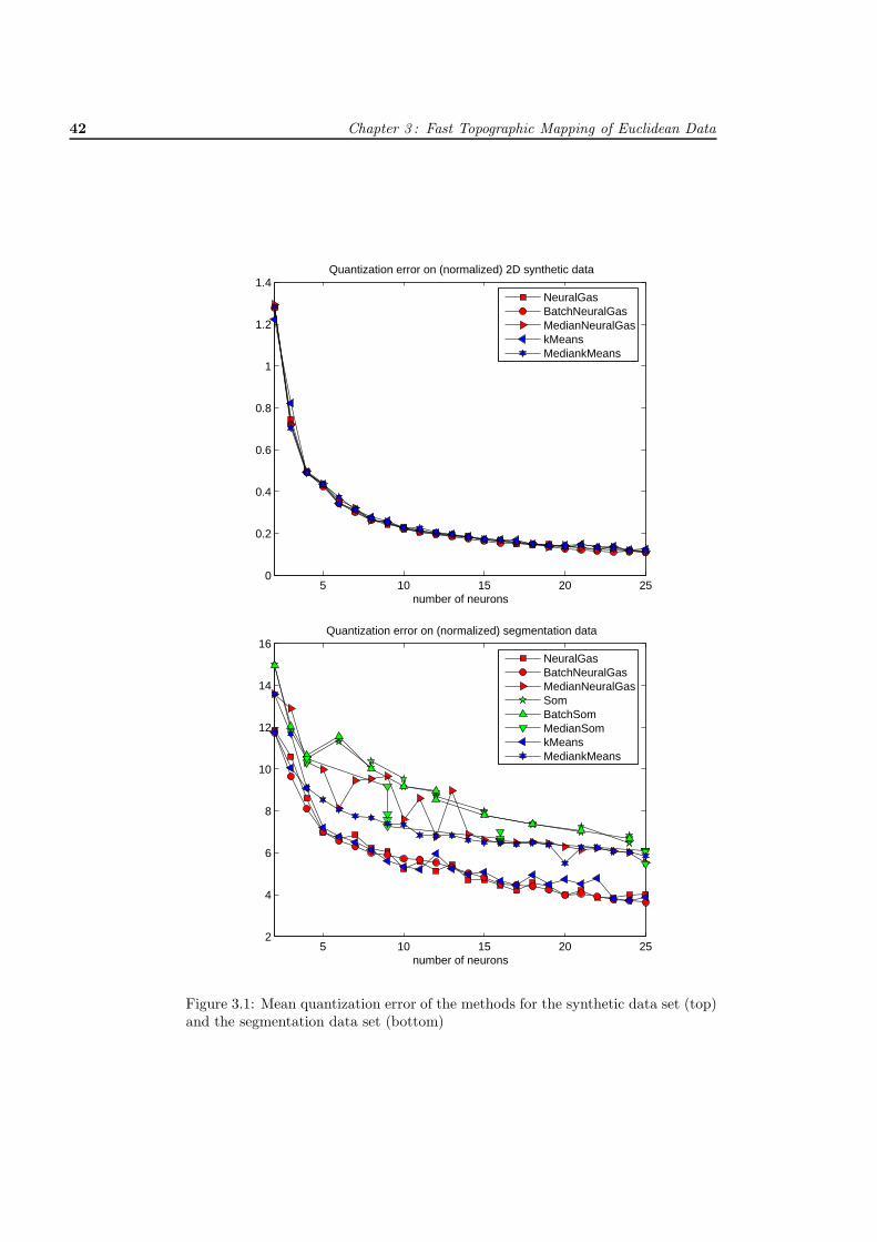
42 Chapter 3 : Fast Topographic Mapping of Euclidean Data
5 10 15 20 250
0.2
0.4
0.6
0.8
1
1.2
1.4Quantization error on (normalized) 2D synthetic data
number of neurons
NeuralGasBatchNeuralGasMedianNeuralGaskMeansMediankMeans
5 10 15 20 252
4
6
8
10
12
14
16Quantization error on (normalized) segmentation data
number of neurons
NeuralGasBatchNeuralGasMedianNeuralGasSomBatchSomMedianSomkMeansMediankMeans
Figure 3.1: Mean quantization error of the methods for the synthetic data set (top)and the segmentation data set (bottom)

3.5 Experimental Results and Applications 43
-1.5 -1 -0.5 0 0.5 1 1.5-2
-1.5
-1
-0.5
0
0.5
1
1.5
2
-1.5 -1 -0.5 0 0.5 1 1.5-2
-1.5
-1
-0.5
0
0.5
1
1.5
2
Figure 3.2: Receptive fields obtained by BNG (left) and SBNG (right) on an artifi-cial two-dimensional data set. Obviously, the incorporation of the label informationfor SBNG yields a better separation of the two classes; the prototype locationsfollow the classification boundary.
0.1 0.3 0.5 0.7 0.90.88
0.9
0.92
0.94
0.96
0.98
SNG TrainSNG TestBSNG TrainBSNG Test
Figure 3.3: Accuracy on the training and test set achieved by Supervised Batch NG(SBNG) and Batch NG (BNG) on the iris dataset for different mixing parametersβ.

44 Chapter 3 : Fast Topographic Mapping of Euclidean Data
0.1 0.3 0.5 0.7 0.90.935
0.945
0.955
0.965
0.975
0.98
SNG Train
SNG Test
BSNG Train
BSNG Test
Figure 3.4: Accuracy on the training and test set achieved by Supervised Batch NG(SBNG) and Batch NG (BNG) on the Wisconsin breast cancer dataset for differentmixing parameters β.
-1 0 1 2 33.8
3.82
3.84
3.86
3.88
3.9
3.92
3.94
d = 1
d = 2
d = 3
Figure 3.5: Entropy of map formation for different values c of magnification controland training sets of intrinsic dimensionality d ∈ {1, 2, 3}. The arrows indicate theexpected optima of the entropy according to the underlying theory.

3.5 Experimental Results and Applications 45
0 50 100 150 200 250 3000
50
100
150
200
250
300
Figure 3.6: Final prototype location for α = 0.01
0 50 100 150 200 250 3000
50
100
150
200
250
300
Figure 3.7: Final prototype location for α = 0.61
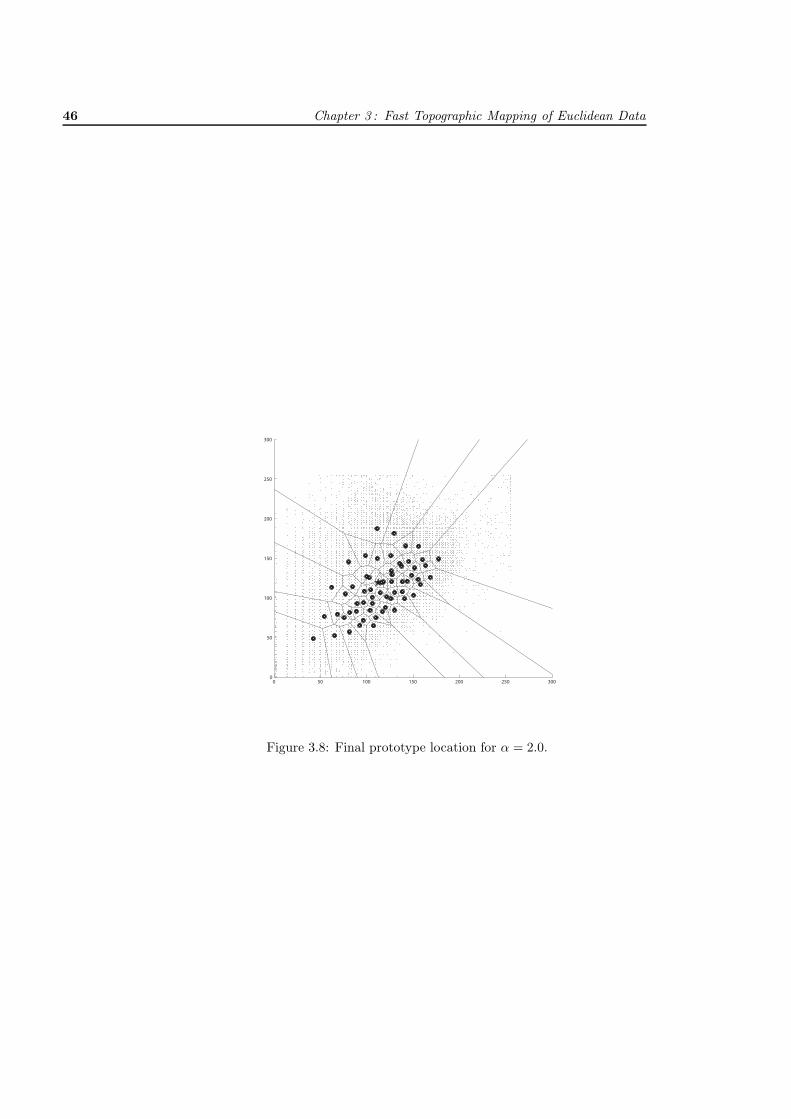
46 Chapter 3 : Fast Topographic Mapping of Euclidean Data
0 50 100 150 200 250 3000
50
100
150
200
250
300
Figure 3.8: Final prototype location for α = 2.0.

3.5 Experimental Results and Applications 47
0 100 200 3000
100
200
300Class 1
0 100 200 3000
100
200
300Class 4
0 100 200 3000
100
200
300Class 7
0 100 200 3000
100
200
300Class 10
0 100 200 3000
100
200
300Class 13
0 100 200 3000
100
200
300Class 2
0 100 200 3000
100
200
300Class 5
0 100 200 3000
100
200
300Class 8
0 100 200 3000
100
200
300Class 11
0 100 200 3000
100
200
300Class 14
0 100 200 3000
100
200
300Class 3
0 100 200 3000
100
200
300Class 6
0 100 200 3000
100
200
300Class 9
0 100 200 3000
100
200
300Class 12
0 100 200 3000
100
200
300All data
Figure 3.9: Location of the classes on the map: a large overlap of the classes can beobserved since many classes are centered around different kinds of forest. Classes 9(water) and 14 (alpine vegetation) , respectively, constitute two extremal classes atthe borders.

48 Chapter 3 : Fast Topographic Mapping of Euclidean Data
-1 0 1 2 30
5
10
15
20Class 1
-1 0 1 2 30
5
10
15
20Class 4
-1 0 1 2 30
5
10
15
20Class 7
-1 0 1 2 30
5
10
15
20Class 10
-1 0 1 2 30
5
10
15
20Class 13
-1 0 1 2 30
5
10
15
20Class 2
-1 0 1 2 30
5
10
15
20Class 5
-1 0 1 2 30
5
10
15
20Class 8
-1 0 1 2 30
5
10
15
20Class 11
-1 0 1 2 30
5
10
15
20Class 14
-1 0 1 2 30
5
10
15
20Class 3
-1 0 1 2 30
5
10
15
20Class 6
-1 0 1 2 30
5
10
15
20Class 9
-1 0 1 2 30
5
10
15
20Class 12
-1 0 1 2 30
5
10
15
20All classes
Figure 3.10: Number of neurons per class in dependence of the control parameterc.

3.5 Experimental Results and Applications 49
Figure 3.11: Mixture of four Gaussian clusters
Figure 3.12: Checkerboard data

50 Chapter 3 : Fast Topographic Mapping of Euclidean Data
Figure 3.13: 11 clouds data set given by a mixture of Gaussians.
-2 -1.5 -1 -0.5 0 0.5 1 1.5 2-2
-1.5
-1
-0.5
0
0.5
1
1.5
2
-2 -1.5 -1 -0.5 0 0.5 1 1.5 2-2
-1.5
-1
-0.5
0
0.5
1
1.5
2
Figure 3.14: Results of patch clustering for i.i.d. data representations (randomlysampled from all clusters) after the first (left) and last (right) patch. The datapresented in the patch are highlighted. Obviously, the cluster centers are almostfixed after the first patch due to the nature of the problem.

3.5 Experimental Results and Applications 51
-2 -1.5 -1 -0.5 0 0.5 1 1.5 2-2
-1.5
-1
-0.5
0
0.5
1
1.5
2
-2 -1.5 -1 -0.5 0 0.5 1 1.5 2-2
-1.5
-1
-0.5
0
0.5
1
1.5
2
-2 -1.5 -1 -0.5 0 0.5 1 1.5 2-2
-1.5
-1
-0.5
0
0.5
1
1.5
2
-2 -1.5 -1 -0.5 0 0.5 1 1.5 2-2
-1.5
-1
-0.5
0
0.5
1
1.5
2
-2 -1.5 -1 -0.5 0 0.5 1 1.5 2-2
-1.5
-1
-0.5
0
0.5
1
1.5
2
-2 -1.5 -1 -0.5 0 0.5 1 1.5 2-2
-1.5
-1
-0.5
0
0.5
1
1.5
2

52 Chapter 3 : Fast Topographic Mapping of Euclidean Data
-2 -1.5 -1 -0.5 0 0.5 1 1.5 2-2
-1.5
-1
-0.5
0
0.5
1
1.5
2
-2 -1.5 -1 -0.5 0 0.5 1 1.5 2-2
-1.5
-1
-0.5
0
0.5
1
1.5
2
-2 -1.5 -1 -0.5 0 0.5 1 1.5 2-2
-1.5
-1
-0.5
0
0.5
1
1.5
2
-2 -1.5 -1 -0.5 0 0.5 1 1.5 2-2
-1.5
-1
-0.5
0
0.5
1
1.5
2
-2 -1.5 -1 -0.5 0 0.5 1 1.5 2-2
-1.5
-1
-0.5
0
0.5
1
1.5
2
Figure 3.15: Results of patch clustering for data presented consecutively mode-wiseaccording to its location in the data set (from left to right and top to bottom)after every patch. The data presented in each patch is highlighted. As can beclearly observed, the cluster centers vary in every patch, however, they are locatedat almost ideal position with respect to all already processed data, resulting in analmost perfect clustering after the final patch.

3.5 Experimental Results and Applications 53
-2 -1.5 -1 -0.5 0 0.5 1 1.5 2-2
-1.5
-1
-0.5
0
0.5
1
1.5
2
-2 -1.5 -1 -0.5 0 0.5 1 1.5 2-2
-1.5
-1
-0.5
0
0.5
1
1.5
2
-2 -1.5 -1 -0.5 0 0.5 1 1.5 2-2
-1.5
-1
-0.5
0
0.5
1
1.5
2
-2 -1.5 -1 -0.5 0 0.5 1 1.5 2-2
-1.5
-1
-0.5
0
0.5
1
1.5
2
-2 -1.5 -1 -0.5 0 0.5 1 1.5 2-2
-1.5
-1
-0.5
0
0.5
1
1.5
2
-2 -1.5 -1 -0.5 0 0.5 1 1.5 2-2
-1.5
-1
-0.5
0
0.5
1
1.5
2

54 Chapter 3 : Fast Topographic Mapping of Euclidean Data
-2 -1.5 -1 -0.5 0 0.5 1 1.5 2-2
-1.5
-1
-0.5
0
0.5
1
1.5
2
-2 -1.5 -1 -0.5 0 0.5 1 1.5 2-2
-1.5
-1
-0.5
0
0.5
1
1.5
2
-2 -1.5 -1 -0.5 0 0.5 1 1.5 2-2
-1.5
-1
-0.5
0
0.5
1
1.5
2
-2 -1.5 -1 -0.5 0 0.5 1 1.5 2-2
-1.5
-1
-0.5
0
0.5
1
1.5
2
-2 -1.5 -1 -0.5 0 0.5 1 1.5 2-2
-1.5
-1
-0.5
0
0.5
1
1.5
2
Figure 3.16: Results of patch clustering for data presented according to its locationin the data set subject to a diffusion process (from left to right and top to bottom,mode-wise presentation with parts of the current, the two preceding, and the twosubsequent clusters) after every patch. The data presented in each patch is high-lighted. As before, the cluster centers vary in every patch. After processing the fulldata set, the cluster centers are located at almost ideal position with respect to allalready processed data. Apart from a small shift of the center of cluster 7 whichdoes not effect its receptive field in the given data set, an almost perfect clusteringafter the final patch is achieved.

Chapter 4
Topographic Mapping ofDissimilarity Data
In this chapter we are concerned with the processing of data that is in general notof Euclidean nature, that means an explicit embedding into Euclidean spaces is notavailable. The classical prototype-based topographic mapping methods introducedabove cannot handle these data since their original formulations are based on vectoroperations in Euclidean spaces. In what follows, we will extend the principles of theabove introduced prototype-based methods to handle those non-vectorial datasets.For the sake of clarity, the techniques are once again demonstrated exemplarily forNeural Gas, but a transfer of the ideas to Self-Organizing Maps is obvious and shallbe sketched where necessary.
4.1 Introduction to Dissimilarity Data
As the name suggests, dissimilarity describes a certain degree of difference betweenobjects that might be measured by arbitrary values. Dissimilarities are not requiredto be distances in a sense that they are metric. We only expect them to be symmet-ric and nonnegative, what is certainly a natural demand.1 Also an object shouldbe self-similar, so we require the dissimilarity to itself to be zero. We formalizedissimilarities by the following definition of dissimilarity measures.
Dissimilarity Measures Given a set of data points V from an arbitrary space.A function d : V × V →� is a dissimilarity measure on V , if it is non-negative,reflexive, and symmetric. That is, for all v, v′ ∈ V it holds
• d(v, v′) ≥ 0 (non-negativity),
• d(v, v′) = 0 (reflexivity), and
• d(v, v′) = d(v′, v) (symmetry).
For convenience, we denote the dissimilarity measure d(vi, vj) defined on a finitedataset V = {v1, v2, . . . , vm} also as dij in the following when it can be done withoutambiguity. �
So by definition, the Euclidean metric is obviously a dissimilarity measures.Further examples of dissimilarity measures used in practical applications are, forinstance,
1Although in the context of psychological experiments there are different opinions whether thedemand of symmetry might be too restrictive.
55

56 Chapter 4 : Topographic Mapping of Dissimilarity Data
• alignment distances from bioinformatics,
• Levenshtein metric from string processing,
• Hamming distance from information theory,
• geodesic distance from geometry,
• Jaccard index and Tanimoto coefficient from statistics, and
• normalized compression distance from algorithmic information theory.
Note that for a finite set V = {v1, v2, . . . , vm} of data points the dissimilaritymeasure can be written as a dissimilarity matrix D = (dij)ij . Typically, we willuse this representation in the following. The set of data points and the structure ofthe underlying mathematical space is in general unknown, in almost all cases onlya dissimilarity matrix is given. For historical reasons, dissimilarity datasets are alsocalled relational data (cf. Hathaway and Bezdek, 1994), because relations betweenobjects are described.
It is to be understood here, that dissimilarity data does not necessarily originatefrom a Euclidean vector space. Even if given data stems from a metric space, likedata gained from Levenshtein metric or alignment distances for instance, it is ingeneral not isometrically embeddable into any Euclidean space (Matousek, 2002;Indyk and Matousek, 2004; Pekalska and Duin, 2005). So almost all of the abovepresented dissimilarity measures are in general non-Euclidean. It is still an activefield of mathematical research which structures are isometrically embeddable into aEuclidean space and which are not, and if they are not, the question arises what arethe bounds on the distortion that has to be accepted for any embedding (cf. Ma-tousek, 2007).
Gram Matrices Given a finite dataset X ⊂ �m×d from a Euclidean space,the corresponding Gram matrix G = XXT = (〈xi xj〉)ij containing the pairwisestandard inner products is always positive definite.
In the following, Gram matrices of indefinite inner products for non-Euclideanspaces are constructed and their eigenspectra are analyzed. It will turn out thatdissimilarity datasets are characterized by the eigenspectra of their correspondingGram matrices, namely the respective number e+ and e− of positive and negativeeigenvalues indicate the ratio between Euclidean and non-Euclidean character ofthe data.
Let Im denote the identity matrix of order m, 1m = (1, 1, . . . , 1)T the vectorof order m, and let J = I − 1
m · 1m1Tm. Furthermore, we denote the element-wise
square operation on a matrix A by A�2 =(a2
ij
)ij
.The corresponding Gram matrix G of a dissimilarity matrix D is then defined
to be
G = −12JD�2J. (4.1)
The inertia of Gram matrix G is defined to be the triple (e+, e−, e0) in whiche+, e−, and e0 are the respective number of positive, negative, and zero eigenvalues,counting algebraic multiplicities. The inertia is invariant under congruence trans-formations and it can be shown that if G has inertia (p, q, z) then there exists a

4.1 Introduction to Dissimilarity Data 57
basis transformation with basis S such that SGST = H , written G � H , where
H =
⎛⎜⎝ Ip
−Iq
0z
⎞⎟⎠ (cf. Meyer, 2000). (4.2)
It should be mentioned here, that the corresponding Gram matrix G with inertia(p, q, z) of a given dissimilarity dataset, as an indefinite inner product matrix, canalways be represented by a set of points X in a suitable Euclidean space �p+q
such that G = ((xi|Hxj))ij = XHXT , where H � G is defined as above, and (.|.)denotes the standard inner product (cf. Gohberg et al., 2005). This representationleads to the theory of pseudo-Euclidean spaces (Goldfarb, 1984), that shall not beconsidered further within this work.
Later on in the experimental section, Table 4.2 shows the inertia of severalnon-Euclidean datasets that are used in the experiments. Moreover, the sortedeigenspectra of the Gram matrices can be visualized as it is done on page 82 to gaindeeper insights into the structure of the non-Euclidean datasets.
Obviously, the prototype-based topographic mapping methods introduced in theprevious chapter cannot handle dissimilarity data since they are based on vectorialupdates. At first feel, a solution would be the prior embedding of given dissimilaritydata into a Euclidean space accepting some distortion. But this approach is mostof the times impracticable because embeddings of good quality are often computa-tionally hard to get (cf. Matousek, 2007).
Spread Transform An alternative approach proposed by Hathaway and Bezdek(1994) for their NERF c-means algorithm relies on a spread transformation of thedissimilarity matrices that converts them to Euclidean distance matrices by
Dγ = D + γ · (1m1Tm − Im)
for a suitable parameter γ > 0. Their method then operates directly on the gen-erated Euclidean distances. However, as discussed later on, the spreading transfor-mation alters the data space significantly in an unprofitable way.
It can be shown, see (Gower and Legendre, 1986), that the minimum spreadingvalue to make a given dissimilarity matrix D Euclidean is given by the largesteigenvalue of the matrix(
0m −JD�2J
−Im −2JDJ
),
where Im denotes the identity matrix of order m, and J = I − 1m · 1m1T
m.
This technique is also used by Roth et al. (2003) to transform dissimilarities intosquared Euclidean distance matrices. Let emin(.) denote the minimum eigenvalueof a given matrix. To make D squared Euclidean, the minimum spreading value is2 · emin(1
2JDJ).
In the experimental section, Table 4.3 shows the minimum spreading values forthe used datasets to become squared Euclidean or Euclidean, respectively.
It should be noted here, that the spreading transformation distorts the originaldissimilarities in a way that the structure of the data space can change considerably.

58 Chapter 4 : Topographic Mapping of Dissimilarity Data
42 44 46 48 50 520
5
10
15
20
25
30
35
40
45
50
41 42 43 44 45 460
5
10
15
20
25
30
35
40
45
50
42 44 46 48 50 520
5
10
15
20
25
30
35
40
45
50
41 42 43 44 45 460
5
10
15
20
25
30
35
40
45
50
42 44 46 48 50 520
5
10
15
20
25
30
35
40
45
50
41 42 43 44 45 460
5
10
15
20
25
30
35
40
45
50
Figure 4.1: Implications of the Spread-Transformation: Local optima of cost func-tion (4.3) reached by repeated runs of Relational Neural Gas (left column) andDeterministic Annealing (right column) on Cat Cortex dataset. First row is onuntouched data, second row on squared-Euclidean spreaded data, and third row onEuclidean spreaded data. The parameters were 5 clusters, 1000 runs, 100 epochsRNG and 300 epochs DA
To empirically demonstrate this effect, we consider the intra-cluster distance, awell-known clustering measure, given by the cost function
E(δ, d) =∑
i
1∑j δij
·∑
j
∑k
δijδikdjk (4.3)
with crisp cluster assignments δij ∈ {0, 1}. It was shown by Roth et al. (2003) thatthe spreading transformation does not alter the local optima of the cost function(4.3), only a constant is added. The global optimization of the cost function is NP-hard (Brucker, 1978), the methods used in the simulation are trying to find goodlocal optima.
As it can be seen from the simulations (cf. Figure 4.1 and Figure 4.2), thealgorithms cannot explore the space efficiently any longer. The distribution of localoptima found by the algorithms over time is altered towards worse local optima.The algorithms even might fail to find the best local optima that they have foundbefore the transformation.
Here, the need for methods arises that are able to process dissimilarity data

4.2 Prototype-based Methods in Non-Euclidean Spaces 59
directly. In the subsequent sections, we will focus on topographic mapping tech-niques for dissimilarity datasets that are based on prototypes and perform exactlyas desired.
Before going into details, we consider briefly a related stochastic approach deal-ing with dissimilarity data that is very popular. A stochastic formulation of Self-Organizing Maps for dissimilarity data was introduced by Graepel and Obermayer(1999). It is based on a cost function which was derived in analogy to the onethat has been proposed by Luttrell (1994) in a general stochastic framework utiliz-ing a folded Markov chain approach and comprising in particular Kohonen’s Self-Organizing Maps. The optimization of the cost function is done by an ExpectationMaximization algorithm (Jaynes, 1957a,b) in combination with a deterministic an-nealing scheme (Rose et al., 1990, 1992; Rose, 1998). A mathematical framework fordeterministic annealing and mean-field approximations in the context of dissimilar-ity data was presented by Hofmann and Buhmann (1999). Successful applicationsof the stochastic approach have been made by Saalbach et al. (2005) to medical datameasured by the Earth Mover’s Distance utilizing a hyperbolic lattice structure.
4.2 Prototype-based Methods inNon-Euclidean Spaces
Up to this point, the introduced methods were based exclusively on Euclideanspaces. But unlike data originating from vector spaces, the important class of rela-tional data is characterized only by pairwise dissimilarities d(vi, vj) given for someunderlying (and in general unknown) data points vi, vj ∈ V . Recall from section 4.1that the only demands made on dissimilarity measures are non-negativity dij ≥ 0,reflexivity dii = 0, and symmetry dij = dji. They are not necessarily metric bynature, and even if given data stems from a metric space, the space might not beisometrically embeddable into any Euclidean space at all (cf. Matousek, 2002).
Obviously, all the classical processing methods as introduced above cannot han-dle relational data since their original formulation is based on prototype updates ina vector space. Now, we are restricted to a discrete space whose structure is char-acterized only by pairwise dissimilarities between its elements. In general, thereare no linear combinations possible and potential prototypes cannot be settled inbetween the data points.
A possible way to circumvent these issues would be accepting a certain degreeof distortion and embed the relational data into a Euclidean space anyway. Amongother techniques, this non-isometrical embedding can be achieved by transformingthe data using a spreading technique (cf. Hathaway and Bezdek, 1994). That way,we end up with Euclidean data points but as discussed above, the structure of thedata space is changing and optimization is getting harder.
In this section, we will follow another way by keeping the given dissimilaritiesas they are and find better suited methods to work directly on them. It will turnout that, for this first approach, we also have to sacrifice a certain amount of ac-curacy. But later on, we will overcome these restrictions by introducing continuousprototype updates.
The key idea of the so-called median approach (Cottrell et al., 2006) is the re-striction of prototype locations to given data points, such that prototype locationsare well defined in the given space.
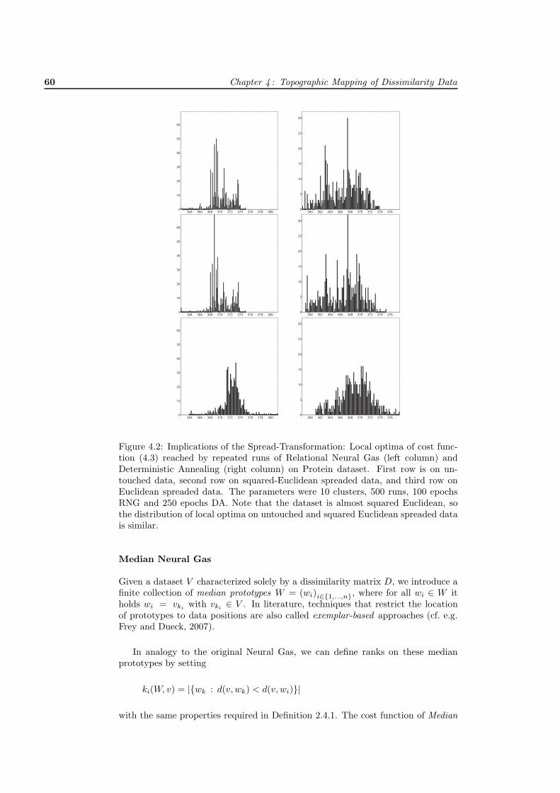
60 Chapter 4 : Topographic Mapping of Dissimilarity Data
364 366 368 370 372 374 376 378 3800
10
20
30
40
50
60
360 362 364 366 368 370 372 374 3760
5
10
15
20
25
30
364 366 368 370 372 374 376 378 3800
10
20
30
40
50
60
360 362 364 366 368 370 372 374 3760
5
10
15
20
25
30
364 366 368 370 372 374 376 378 3800
10
20
30
40
50
60
360 362 364 366 368 370 372 374 3760
5
10
15
20
25
30
Figure 4.2: Implications of the Spread-Transformation: Local optima of cost func-tion (4.3) reached by repeated runs of Relational Neural Gas (left column) andDeterministic Annealing (right column) on Protein dataset. First row is on un-touched data, second row on squared-Euclidean spreaded data, and third row onEuclidean spreaded data. The parameters were 10 clusters, 500 runs, 100 epochsRNG and 250 epochs DA. Note that the dataset is almost squared Euclidean, sothe distribution of local optima on untouched and squared Euclidean spreaded datais similar.
Median Neural Gas
Given a dataset V characterized solely by a dissimilarity matrix D, we introduce afinite collection of median prototypes W = (wi)i∈{1,...,n}, where for all wi ∈ W itholds wi = vki with vki ∈ V . In literature, techniques that restrict the locationof prototypes to data positions are also called exemplar-based approaches (cf. e.g.Frey and Dueck, 2007).
In analogy to the original Neural Gas, we can define ranks on these medianprototypes by setting
ki(W, v) = |{wk : d(v, wk) < d(v, wi)}|
with the same properties required in Definition 2.4.1. The cost function of Median

4.2 Prototype-based Methods in Non-Euclidean Spaces 61
Neural Gas is then given by
Eλ(W ) =n∑
i=1
m∑j=1
hλ(ki(W, vj)) · d(wi, vj)2. (4.4)
For the same reason as given for Batch Neural Gas, we now introduce hidden vari-ables kij to replace the rank function and apply alternating optimization. As before-hand, the optimal assignments are given by the ranks kij = ki(W, v). The optimalprototype locations, however, are now determined by the so-called generalized me-dian (cf. Kohonen and Somervuo, 2002)
w∗i = argmin
vk
∑j
hλ(kij) · d(vj , vk)2 (4.5)
and can be found by exhaustive search. A sketch of the algorithm is given in tableAlgorithm 4.2. It has been shown in (Cottrell et al., 2006) that Median Neural Gasconverges to a (local) optimum of the cost function.
Algorithm 4.1: Median Neural Gas
Input
Dissimilarity matrix D ∈ �m×m
Begin
(* Initialize prototypes *)
Init wi randomly for all i ∈ {1, . . . , n} and λ0 = n/2, λ = λ0
(* Repeat for a given number of epochs. . . *)
for t := 1 to epochs do
Determine ranks (break ties deterministically). . .
ki(W, vj) = |{ l ∈ {1, . . . , n} : d(wl, vj) < d(wi, vj)}|Update prototype locations by generalized median. . .
wi = argminvk
∑j hλ(kij) · d(vj , vk)2
Decrease neighbourhood range. . .
λ = λ0 · (0.01/λ0)t/epochs
endfor;
(* Return representative prototypes *)
Return wi
End.
Despite our focus on Median Neural Gas, it should be noted here, that the me-dian approach can easily be transferred to Self-Organizing Maps (El Golli et al.,2004; Cottrell et al., 2005).
Obviously, the median approach features the inherent drawback that only dis-crete adaptation steps can be performed which can dramatically reduce the repre-sentation quality of the mapping. Furthermore, the complexity of the median batchapproaches is quadratic in the number of data points, what sets up a great obstaclewhen dealing with very large datasets. We will see later on in section 4.2 that this
62 Chapter 4 : Topographic Mapping of Dissimilarity Data
obstacle can be overcome by an elegant patch processing method. For Batch SOMthere are also faster approaches than exhaustive search (Conan-Guez et al., 2006),exploiting characteristics of the grid structure for pre-calculations, reusing earlierresults, and applying early stopping among other intelligent techniques to speed upprocessing.
Another drawback of the median approach is its incapacity to separate proto-types that have been collapsing onto a single location in data space. A quick solutionto the problem consists in adding some noise term to the update rule provoking aseparation by chance. More sophisticated strategies to tackle the issue of collapsingprototypes in median approaches are addressed in (Rossi, 2007) utilizing a branchand bound approach.
Also the integration of additional information can be achieved the same way asdone before. This is realized more precisely in the next section:
Supervised Median Neural Gas
Following Section 3.3, we can also incorporate additional information in form of la-bels given for each data point into the processing of Median Neural Gas (cf. Hammeret al., 2006a). The concept can also easily be migrated to other prototype-basedmedian methods like Median SOM (cf. Hammer et al., 2006a).
Let a dataset V = {v1, v2, . . . , vm} be given indirectly by a dissimilarity measured on V . In addition, there shall be a collection of labels
(vL
i
)i∈{1,...,m} from �c
corresponding to an unary encoding of the classes the data points belong to.Now, we define a new dissimilarity measure
d∗β(vi, vj)2 = (1 − β) · d(vi, vj)2 + β∥∥vL
i − vLj
∥∥2
based on d incorporating also the label space L. Replacing the original dissimilaritymeasure d in the original cost function (4.4) by d∗ yields an extended cost function,namely
E∗λ(W, WL) =
n∑i=1
m∑j=1
hλ(ki(W, vj)) · d∗β(wi, vj)2
= (1 − β) ·n∑
i=1
m∑j=1
hλ(ki(W, vj)) · d(wi, vj)2
+ β ·n∑
i=1
m∑j=1
hλ(ki(W, vj)) ·∥∥wL
i − vLj
∥∥2.
(4.6)
This extended cost function can be optimized by alternating optimization treatingthe different parts separately as shown in Section 3.3.
Note that it can be shown in the same way as presented in (Hammer et al.,2006a) that the Supervised Median Neural Gas algorithm converges.
The introduced modification now allows to incorporate additional informationinto the learning process which turns the original unsupervised methods into super-vised ones. This supervision helps to improve the quality of the results because thereceptive fields are influenced by the underlying class information. Especially, whenthe prototypes are used as a classifier, this leads to a better generalization ability.
As observed beforehand, an important drawback of the median approaches istheir quadratic time complexity in the size of input data. For the processing of

4.2 Prototype-based Methods in Non-Euclidean Spaces 63
very large datasets, arising in numerous fields of applications today, this fact posesa severe limitation of applicability or even the uselessness of the median approaches.
In what follows, we are concerned with an alternative processing scheme thatcircumvents the quadratic time complexity of the median approaches.
Processing of Very Large Dissimilarity Datasets
One of the greatest challenges in data mining today (Yang and Wu, 2006), arisingespecially in the fields of web mining and bioinformatics, is the topographic mappingof very large dissimilarity datasets to explore their structure and gain informationthat otherwise would remain concealed, buried due to the sheer amount of data.These large non-Euclidean datasets cannot be held at once within random-accessmemory during computation, so the batch variants presented above like MedianSelf-Organizing Maps or Median Neural Gas cannot be applied.
Here, we present fast approximate (semi-)supervised versions of SOM and NGfor non-Euclidean data that are able to handle large text datasets by a single passtechnique. The introduced methods are based on patches that can be chosen inaccordance to the size of the available random-access memory. These algorithmsare running in constant space and linear time and provide different visualizations ofthe data space. Moreover, the patch technique opens the way for long-term learningand scalability, what is especially suited for information systems where the databaseis updated perpetually, e.g. in visual search engines etc.
For an illustration of one of the several issues to deal with, we show the storageneeded for dissimilarity matrices due to their quadratic growth in the number ofdata points. The following table shall demonstrate the obvious demands that areposed by some real world large datasets.
Size of Dissimilarity Matrix (Double Precision)
n Size Name of Dataset
5000 190MB Copenhagen Chromosome Dataset10,000 763MB20,000 3.0GB 20 Newsgroup Dataset50,000 18.6GB200,000 300.0GB Large 13 Newsgroup Dataset
Unfortunately, also the time complexity of the Median methods is quadratic. Tocope with very large datasets, it is therefore necessary to accelerate the methodsand reduce their space usage. Fast variants of Median approaches that are able tohandle very large datasets by a single pass technique based on patches chosen inaccordance to the size of the available random-access memory were first introducedby Hasenfuss and Hammer (2008). In the upcoming section, we will introduce thesevariants on the basis of Median Neural Gas, whereby an extension to Median SOMis obvious.
Assume data are given as a dissimilarity matrix D = (dij)i,j=1,...,m with entriesdij = d(vi, vj) representing the dissimilarity of the datapoints vi and vj .
During processing of Patch Median NG, np disjoint patches of fixed size p =�m/np� are taken from the dissimilarity matrix D consecutively,2 where every patch
Pi = (dst)s,t=(i−1)·p+1,...,i·p ∈ �p×p
2The remainder is no further considered here for simplicity. In the practical implementationthe remaining datapoints are simply distributed over the first (M − p · np) patches.

64 Chapter 4 : Topographic Mapping of Dissimilarity Data
is a submatrix of D.The idea of the patch scheme is to add the prototypes from the processing of
the former patch Pi−1 as additional datapoints to the current patch Pi, forming anextended patch P ∗
i to work on further.The additional datapoints – the former prototypes – are weighted according to
the size of their receptive fields, i.e. how many datapoints they have been represent-ing in the former patch. Therefore, every datapoint vj , as a potential prototype, isequipped with a multiplicity mj, that is at first initialized with mj = 1.
But unlike the situation of Patch NG in Euclidean space (Alex et al., 2009),where inter-patch distances can always be recalculated with help of the Euclideanmetric, we are now dealing with an unknown mathematical space. We have toconstruct the extended patch from given dissimilarity data.
Let n be the fixed number of prototypes and let Nk denote the index set ofprototypes of step k pointing onto elements of the dissimilarity matrix D. Theextended patch P ∗
i is then defined as
P ∗i =
⎛⎜⎜⎜⎜⎜⎜⎜⎜⎜⎜⎝
d(Ni−1) d(Ni−1, Pi)
d(Ni−1, Pi)T Pi
⎞⎟⎟⎟⎟⎟⎟⎟⎟⎟⎟⎠
where
d(Ni−1) = (dst)s,t ∈ Ni−1∈ �n×n
d(Ni−1, Pi) = (dst)s ∈ Ni−1,t=(i−1)·p+1,...,i·p ∈ �n×p
denote the inter-distances of former prototypes and the distances between formerprototypes and current patch points, respectively.
Now, the original Median Batch Neural Gas method must be modified to handlethe weighted datapoints. Incorporating the multiplicities into the cost functionyields
E(W ) =n∑
i=1
m∑j=1
hλ(kij) · mj · d(wi, vj)2,
since every datapoint vj is weighted with multiplicity mj . The multiplicity m(wi)of a prototype wi ∈ Wt is given by
m(wi) =∑
v∈P∗t ∩Vi(Wt)
m(v),
the sum of multiplicities of all data points in the receptive field. The new updaterule for the prototypes derived from the modified cost function is
wi = argminvk
p∑j=1
hλ(kij) · mj · d(vj , vk)2.
Picking up the pieces, we yield Algorithm 4.2.

4.2 Prototype-based Methods in Non-Euclidean Spaces 65
Algorithm 4.2: Patch Median Neural Gas (Hasenfuss and Hammer, 2008)
Begin
Cut the first Patch P1
Apply Median Neural Gas on P1 −→ Prototypes N1
Update Multiplicities mj
Repeat for i = 2, . . . , np
Cut patch Pi
Construct Extended Patch P ∗i using Pi and Ni−1
Apply modified Median Neural Gas with Multiplicities
−→ Prototypes Ni
Update Multiplicities mj
Return final prototypes Nnp
End.
Analysis of Complexity
For an analysis of the complexity, we assume at first a fixed patch size p independentof the number of datapoints, as it would be the case when the patch size is chosenaccording to memory limitations. The algorithm then works only on O(m
p · p2) =O(m · p) = O(m) entries of the dissimilarity matrix, compared to O(m2) in theoriginal Median NG method. Moreover, the algorithm uses at most O(p2) = constentries at a specific point in time.
In case of a fixed patch size, also the time complexity is linear, because theMedian NG step is O(p2) what results in O(p2 · m
p ) = O(p · m) = O(m), anadvantage compared to the O(m2) time complexity of the original Median NG.
For a fixed dataset the total number of dissimilarity matrix elements touchedduring processing, compared to an imaginary application of Median NG, is de-creasing in a reciprocal manner for an increasing number of patches. For sake ofsimplicity, we assume here w.l.o.g. that m is completely divisible by p. In detail,for a patch size p chosen independent of the size of the dataset m, the algorithmperforms m
p · p · n log n + p2 = m(n log n + p) ∈ O(m) steps. The original MedianNG in contrast would require m · (n log n + m) ∈ O(m2) processing steps. So theratio
m(n log n + p)m · (n log n + m)
=n logn + m
pn
n log n + m= const + const′ · 1
pn
is a reciprocal function in the number of patches pn.Therefore the method does not only overcome the problem of limited memory,
it also accelerates the processing of datasets, what might be useful in time criticalapplications.
These advantages in space and time complexity are obviously paid back by aloss of accuracy, what is also affirmed in the experiments later on, but the loss turnsout to be small on realistic datasets. Theoretical bounds are not easily obtainable,this is still subject of ongoing research.
Obviously, the above argumentation does not hold if the patch size depends onthe number of datapoints.

66 Chapter 4 : Topographic Mapping of Dissimilarity Data
4.3 Continuous Prototype Updates for Dissimilar-
ity Data
The restriction of prototypes to data point locations as used for the Median tech-niques may induce additional distortion particularly when the data space is sparse.This effect can easily be observed in comparative experiments versus the originalBatch Neural Gas on Euclidean datasets. This drawback of the Median approachesmotivates further research on the possibilities of continuous updates in non-vectorspaces.
First steps towards a continuous update of prototypes were made by Hasen-fuss et al. (2007) with the intention to represent prototypes as combinations ofdata points. Later on, the same authors introduced Relational Neural Gas (RNG)(Hammer and Hasenfuss, 2007) that overcomes the problem of discrete adaptationsteps by using convex combinations of Euclidean embedded data points as proto-types. That way, distance calculations between prototypes and data can be donewithout any knowledge about the embedding. The idea of relational prototypes wasextended to Relational SOM by Hasenfuss and Hammer (2007).
In what follows next, we are concerned with an overview about the relationalapproach. Later on, in the succeeding sections we shall discuss the concepts in moredetail.
For that purpose, we assume that there exists a set of (in general unknown andpresumably high dimensional) Euclidean points V such that dij = ‖vi − vj‖ for allvi, vj ∈ V holds, i.e. we assume there exists an (unknown) isometric embeddinginto a Euclidean space. The key observation is based on the fact that, under theassumptions made, the squared distances ‖wi − vj‖2 between (unknown) embed-ded data points and optimum prototypes can be expressed just in terms of knowndistances dij .
The prototypes in the relational approach are expressed as wi =∑
j αijvj
with∑
j αij = 1. Given a coefficient matrix (αij) ∈ �n×m and a matrix D�2 =(d2
ij
) ∈ �m×m of squared distances, it then holds
‖wi − vj‖2 = (αi∗ · D�2)j − 12· αi∗D�2αT
i∗ (4.7)
what is verified later on in Section 4.3. It should be emphasized here, that thanks to(4.7) the squared distances can be calculated without explicit knowledge of pointsfrom V . Because of this fact, we are able to substitute all terms ‖wi − vj‖2 inBatch NG and Batch SOM by (4.7) and derive new update rules working only ondistances. This allows to reformulate the batch optimization schemes in terms ofrelational data.
Note that, if an isometric embedding into Euclidean space exists, these schemesare exactly equivalent to the batch schemes and will yield identical results. Oth-erwise, the consecutive optimization scheme can still be applied on non-Euclideandata that is not isometrically embeddable into any Euclidean space.
By now, relational methods have been shown beneficial in the field of bioinfor-matics (cf. Hammer et al., 2007a), text processing (cf. Hasenfuss et al., 2008a), andvisualization of discrete musical data (cf. Mokbel et al., 2009).
In the upcoming sections, we will introduce the relational approach in moredetails.

4.3 Continuous Prototype Updates 67
Representation of Distances
In what follows, a representation of distances between relational prototypes anddata points is derived that does not include any knowledge about the data but thedistance matrix. The section is based on the work of Hathaway and Bezdek (1994)who relied on earlier works of Torgerson (1958) and Young and Householder (1938).
Theorem 4.3.1 (Distances between Convex Combinations) Let V be a realinner-product space and V = {v1, v2, . . . , vm} a finite subset of V . Let ‖�‖ =
√〈� �〉denote the canonical norm on V . Furthermore, we denote the matrix of squaredpairwise distances of V by
D�2 =(‖vi − vj‖2
)ij
∈ �m×m.
(a) For the squared pairwise distances between convex combinations over V , i.e.for elements
wi =m∑
j=1
αijvj (where αij ≥ 0 for all i,j andm∑
j=1
αij = 1 for all i),
the following identity holds
‖wi − wj‖2 = αi∗D�2αTj∗ −
12αi∗D�2αT
i∗ −12αj∗D�2αT
j∗. (4.8)
(b) For an element v ∈ V , the distance to a convex combination wi =∑m
j=1 αijvj
over V is given by
‖v − wi‖2 =∑
j
αij‖v − vj‖2 − 12αi∗D�2αT
i∗. (4.9)
Remark Note that the squared distances to convex combinations over V can beexpressed without using the elements from set V directly, only the squared distancesand the coefficients are considered. Thus, the theorem provides a way to handledistance calculations for a set of unknown underlying points, only the squared dis-tances have to be known. Since this situation occurs most of the times in realapplications dealing with non-vectorial datasets, Theorem 4.3.1 turns out to be thekey to sophisticated methods on dissimilarity data.
Proof. (a) In the first step, ‖wi − wj‖2 will be expressed by inner-products.Then, these inner-products will be replaced by distances of elements from V ap-plying the technique of completing the square and using the identity ‖x − y‖2 =〈x − y x − y〉 = 〈x x〉−2 · 〈x y〉+ 〈y y〉. Converting the terms into matrix notationusing D�2
ij = ‖vi − vj‖2 will complete the proof.

68 Chapter 4 : Topographic Mapping of Dissimilarity Data
It directly follows
‖wi − wj‖2 = ‖∑
k
αikvk −∑
k
αjkvk‖2
=
⟨∑k
αikvk
∑k
αikvk
⟩− 2 ·
⟨∑k
αikvk
∑k
αjkvk
⟩+
⟨∑k
αjkvk
∑k
αjkvk
⟩=
∑k
∑l
αikαil 〈vk vl〉︸ ︷︷ ︸=: A(i,j)
−2 ·∑
k
∑l
αikαjl 〈vk vl〉 +∑
k
∑l
αjkαjl 〈vk vl〉︸ ︷︷ ︸=: B(i,j)
= A(i, j) + B(i, j) − 2 ·∑
k
∑l
αikαjl 〈vk vl〉 +∑
k
∑l
αikαjl 〈vk vk〉
+∑
k
∑l
αikαjl 〈vl vl〉−∑
k
∑l
αikαjl 〈vk vk〉︸ ︷︷ ︸=: C(i,j)
−∑
k
∑l
αikαjl 〈vl vl〉︸ ︷︷ ︸=: D(i,j)
=∑
k
∑l
αikαjl‖vk − vl‖2 + (A(i, j) + C(i, j)) + (B(i, j) + D(i, j))
=∑
k
∑l
αikαjl‖vk − vl‖2 − 12
∑k
∑l
αikαil‖vk − vl‖2 − 12
∑k
∑l
αjkαjl‖vk − vl‖2
= αi∗D�2αTj∗ −
12αi∗D�2αT
i∗ −12αj∗D�2αT
j∗.
Because, it holds
−(A(i, j) + C(i, j)) =∑
k
∑l
αikαjl 〈vk vk〉 −∑
k
∑l
αikαil 〈vk vl〉
=12
∑k
∑l
αikαjl 〈vk vk〉 −∑
k
∑l
αikαil 〈vk vl〉 +12
∑k
∑l
αikαjl 〈vk vk〉
(∗)=
12·[∑
k
∑l
αikαjl 〈vk vk〉 − 2 ·∑
k
∑l
αikαil 〈vk vl〉 +∑
k
∑l
αikαil 〈vl vl〉]
=12
∑k
∑l
αikαil ( 〈vk vk〉 − 2 〈vk vl〉 + 〈vl vl〉 )
=12
∑k
∑l
αikαil‖vk − vl‖2
=12αi∗D�2αT
i∗
and similar −(B(i, j) + D(i, j)) = 12αj∗D�2αT
j∗.
In step (∗), the following identity was used,
C(i, j) =∑
k
∑l
αikαjl 〈vk vk〉 =∑
k
αik 〈vk vk〉 =∑
k
∑l
αikαil 〈vk vk〉 ,
that holds because it is∑
t αst = 1 for all s ∈ {1, 2, . . . , n} and therefore it can beleft away or substituted arbitrarily in the above situation.
(b) Applying the same technique as in part (a), it is
‖v − wi‖2 = ‖v −∑
j
αijvj‖2 =∑
j
αij [〈v v〉 − 2 · 〈v vj〉 + 〈vj vj〉]
+
⎛⎝∑
k
∑l
αikαil 〈vk vl〉 −∑
j
αij 〈vj vj〉⎞⎠ =
∑j
αij‖v − vj‖2 + (A(i, j) + C(i, j))
=∑
j
αij‖v − vj‖2 − 12αi∗D�2αT
i∗.

4.3 Continuous Prototype Updates 69
�
Corollary 4.3.2 (Simplified Representation) For the squared distance of anelement vk of a set V = {v1, v2, . . . , vm} to any convex combination wi =
∑mj=1 αijvj
over V , the following simplified identity holds:
‖wi − vk‖2 = (αi∗ · D�2)k − 12· αi∗D�2αT
i∗ (4.10)
Proof. A point vk of the set V = {v1, v2, . . . , vm} can be seen as a convex combi-nation vk =
∑mj=1 δkjvj , where δij denotes the Kronecker delta.
Let δk∗ = (0, . . . , 0, 1, 0, . . . , 0) denote the corresponding coefficient vector. It
then holds ‖wi−vk‖2 = ‖∑mj=1 αijvj−
∑mj=1 δkjvj‖ (4.8)
= αi∗D�2δTk∗− 1
2 ·αi∗D�2αTi∗−
12 · δk∗D�2δT
k∗ = (αi∗ · D�2)k − 12 · αi∗D�2αT
i∗, since (δk∗ · D�2) · δTk∗ = D�2
k∗ · δTk∗ = 0
and also D�2kk = 0. �
Having proved the above theorems for real inner product space, naturally thequestion arises whether there are interesting real inner product spaces to deal with inMachine Learning. Since every normed vector space can be completed to a Banachspace, every real inner product space (as a normed space) can be completed to areal Hilbert space. In turn, every finite dimensional real Hilbert space is norm-isomorphic to a Euclidean space of the same dimension. That means, every realinner product space is isometrically embeddable into a Euclidean space. For thatreason, we will focus our further discussion on Euclidean spaces and non-Euclideanspaces, leaving away the subtleties of norm-isomorphic abstract spaces in between.
Relational Duals of Prototype-based Methods
In the following, we will establish a dual formulation of Batch Neural Gas for dis-similarity data. If given data is isometrically embeddable into a Euclidean space,the dual formulation will generate exactly the same results as Batch NG would dowhen applied to the corresponding points in Euclidean space.
Furthermore, if no Euclidean embedding exists, the algorithm can still be appliedsuccessfully.
Relational Neural Gas (Hammer and Hasenfuss, 2007)
Let there be unknown Euclidean data points V = {v1, v2, . . . , vm} described onlyby squared distances D�2 =
(‖vi − vj‖22
)ij
. For a dual formulation of Batch NeuralGas given only distances, we assume that relational prototypes are expressed asconvex combinations of data points. Without loss of generality, we define
wi =m∑
j=1
αijvj (4.11)
with coefficients αij ≥ 0 for all i,j and∑m
j=1 αij = 1 for all i ∈ {1, . . . , n}.
Due to the nature of the update rule (cf. Eq. (3.5)), prototypes generated byany processing step of Batch Neural Gas are always situated in the convex hull ofdata, so the definition includes all potential prototype locations in the embeddingspace.

70 Chapter 4 : Topographic Mapping of Dissimilarity Data
Also note, that relational prototypes are always defined on a set of points whichwe will refer to as the spanning set, because all possible relational prototype loca-tions are situated in the convex hull spanned by those points.
The update rule of the dual formulation is now given by
αij =hλ(kij)∑j hλ(kij)
(4.12)
for all i ∈ {1, . . . , n} and j ∈ {1, . . . , m}, because inserting Eq. (4.12) into therelational prototype definition Eq. (4.11) yields the same outcome as the originalupdate rule Eq. (3.5), it is
wi =m∑
k=1
αikvk(4.12)=⇒ wi =
m∑k=1
(hλ(kik)∑j hλ(kij)
)vk = Eq. (3.5).
Relational Neural Gas, the dual formulation of Batch NG, handles data givenonly as distances by performing an alternating optimization using the identity fromequation (4.10) to determine the ranks and the dual update rule (4.12) to updatethe relational prototypes, see table Algorithm 4.3 for a sketch of the algorithm.
Algorithm 4.3: Relational Neural Gas
Input
Matrix D�2 ∈ �m×m of squared dissimilarities for (unknown) data points v1, . . . , vm
Begin
(* Initialize relational prototypes wi =∑
j αijvj *)
Init αij ∈ �n×m randomly,
where∑
j αij = 1 for all i ∈ {1, . . . , n} and λ0 = n/2, λ = λ0
(* Repeat for a given number of epochs. . . *)
for t := 1 to epochs do
Compute squared dissimilarities. . .
d(wi, vj) = (αi∗ · D�2)j − 12 · αi∗D�2αT
i∗Determine ranks (break ties deterministically). . .
ki(W, vj) = |{ l ∈ {1, . . . , n} : d(wl, vj) < d(wi, vj)}|Update prototype locations. . .
αij = hλ(ki(W, vj))/∑
l hλ(ki(W, vl))
Decrease neighbourhood range. . .
λ = λ0 · (0.01/λ0)t/epochs
endfor;
(* Return representative prototypes *)
Return αij
End.

4.3 Continuous Prototype Updates 71
Convergence Properties of Relational Neural Gas
In the Euclidean case the convergence properties transfer from the standard batchvariants to the relational approach. That is given data points V = {v1, v2, . . . , vm},a dissimilarity measure d, and let D�2 =
(d(vi, vj)2
)ij
. If (V, d) is isometricallyembeddable into a Euclidean space, Relational NG on D�2 will generate exactlythe same sequence {Wt}t of prototypes while processing as Batch NG does on V asdiscussed above.
Even if we replace the metric ‖x− y‖ by a general dissimilarity measure d(x, y)in all preceding formulas, i.e. a general dissimilarity dataset is given, the relationalmethods will still generate meaningful results as can be seen best from a dualformulation of the cost function (4.14) introduced in the following section. But itmust be stated here that the relational methods might converge to a saddle pointof the cost function, and not always end up in a local optimum like for Euclideanembeddable data. A theoretical framework of convergence and optimality in thenon-Euclidean case is still subject of ongoing research and will not be consideredhere further.
Complexity Issues
Like the median techniques, the serious drawback of the relational approach is itsquadratic time complexity. One solution utilizing a sparse prototype representationwas presented by Rossi et al. (2007). It reduces time complexity by approximat-ing relational prototypes by fewer spanning points and therefore slightly raises thequantization error. Another technique that also accelerates the relational methodsis discussed in a subsequent section. It is based on patches of fixed size and iscapable of processing very large datasets that do not fit into memory at once.
The space needed to store the prototypes of the relational methods is O(n ·m),what is higher compared to the standard approach.
Dual Cost Functions
As introduced in section 3.1, Batch Neural Gas is based on an alternating optimiza-tion scheme, alternately optimizing rank assignments and prototype locations. Inthe following section, we will demonstrate that the original cost function of BNG canbe related to a dual formulation that can be interpreted as a dual constrained opti-mization problem of the intra-cluster distance. For converged prototypes of BatchNeural Gas the original cost function and the dual one with corresponding assign-ments have the same outcome. Moreover, the dual formulation also relates NeuralGas to Deterministic Annealing (Hofmann and Buhmann, 1999) which optimizesthe dual formulation. We derive the dual formulation as follows:
For fixed ranks ki(W, vj) the optimal prototypes w∗i are given by
w∗i =
∑j hλ(ki(W, vj))vj∑j hλ(ki(W, vj))
. (4.13)
For convenience, we abbreviate ki(W, vj) in the following part by kij . Later on inour argumentation, kij will be considered as free parameters of the objective func-tion.
Replacing wi in the cost function (3.1) of BNG by the corresponding optimal
72 Chapter 4 : Topographic Mapping of Dissimilarity Data
prototypes (4.13) of given kij directly yields
E(W ∗, kij) =12
∑i
∑j
hλ(kij)‖w∗i − vj‖2 (4.13)
=12
∑i
∑j
hλ(kij)∥∥∥∥∑
l hλ(kil)vl∑l hλ(kil)
− vj
∥∥∥∥2
=12
∑i
∑j
hλ(kij)(∑
l hλ(kil))2
∥∥∥∥∥∑l
hλ(kil)vl −∑
l
hλ(kil)vj
∥∥∥∥∥2
=12
∑i
∑j
hλ(kij)(∑
l hλ(kil))2 ·⎡
⎣∥∥∥∥∥∑l
hλ(kil)vl
∥∥∥∥∥2
− 2 ·⟨∑
l
hλ(kil)vl
∑l
hλ(kil)vj
⟩+
∥∥∥∥∥∑l
hλ(kil)vj
∥∥∥∥∥2⎤⎦
=12
∑i
1(∑
l hλ(kil))·[∑
s
∑t
hλ(kis)hλ(kit) · (〈vs vt〉 − 2 · 〈vs vt〉 + 〈vt vt〉)]
=12
∑i
1(∑
l hλ(kil))·[∑
s
∑t
hλ(kis)hλ(kit) ·(
12〈vs vs〉 − 〈vs vt〉 +
12〈vt vt〉
)]
=14
∑i
1(∑
l hλ(kil))·[∑
s
∑t
hλ(kis)hλ(kit) · ‖vs − vt‖2
].
Thus, the dual of the cost function (3.1) of Batch NG is given by
14
∑i
1(∑
l hλ(kil))·[∑
s
∑t
hλ(kis)hλ(kit) · ‖vs − vt‖2
]. (4.14)
From the construction it directly follows that for given prototype locations wi andtheir corresponding optimal assignments kij the dual cost function (4.14) has thesame value as the original one (3.1). Note, that the dual formulation is based solelyon the assignments kij and no longer on the distances. The assignments kij cannow be seen as free parameters of a new objective function with the constraint that{k1j , k2j , . . . , knj} is a permutation of {0, 1, . . . , n − 1} for every j ∈ {1, 2, . . . , m}.
As a side effect, the dual cost function constitutes also a descriptive error mea-sure for dissimilarity data to replace the quantization error in non-vectorial spaces.This is an advantage, since only the assignments are needed that could be deriveddirectly from the relational coefficients αij without utilizing the prototype locationswi.
Incorporating Additional Information
Following Section 3.3, we can also incorporate additional information in form of la-bels given for each data point into the relational variants (Hammer and Hasenfuss,2007). As a showcase, we will concentrate on Relational Neural Gas but incorpo-rating additional information into Relational SOM is similar.
Let a dataset V = {v1, v2, . . . , vm} be given indirectly by a dissimilarity measured on V . In addition, there shall be a label vL
j ∈ �c attached to each datapoint vj
corresponding to an unary encoding of the classes the data points belong to.In the context of relational methods as explained above, we assume that the
dataset V is isometrically embeddable into a Euclidean space X = �k for some k.We define a new dissimilarity measure
d∗β(xi, xj)2 = (1 − β) · d(xi, xj)2 + β∥∥xL
i − xLj
∥∥2

4.3 Continuous Prototype Updates 73
on the underlying space X based on d that also incorporates the label space L. Itis based on the original dissimilarity measure d and the Euclidean metric in labelspace L, and that way connects data space X and label space L. Moreover, the newdissimilarity measure d∗β depends on a weighting parameter β ∈ [0, 1], which shallallow us later on to control the influence of the label information on the learningprocess.
In the relational approach, distances between the relational prototypes, betweenrelational prototypes and data points, and also between data points regarded asconvex combinations are according to (4.8) given by
d(xi, xj)2 = αi∗D�2αTj∗ −
12αi∗D�2αT
i∗ −12αj∗D�2αT
j∗,
where D�2 is the matrix of squared dissimilarities.Using this expression to calculate the dissimilarity measure d∗ leads to Algorithm4.3, introduced by Hammer and Hasenfuss (2007).
Algorithm 4.4: Supervised Relational Neural Gas
Input
Matrix D�2 ∈ �m×m of squared dissimilarities for (unknown) data points v1, . . . , vm
Labels{vL1 , vL
2 , . . . , vLm
} ⊂ �c
Begin
(* Initialize relational prototypes wi =∑
j αijvj *)
Init αij ∈ �n×m randomly,
where∑
j αij = 1 for all i ∈ {1, . . . , n} and λ0 = n/2, λ = λ0
(* Repeat for a given number of epochs. . . *)
for t := 1 to epochs do
Compute squared dissimilarities. . .
d∗β(wi, vj) = (1 − β) · ((αi∗ · D�2)j − 12 · αi∗D�2αT
i∗)
+ β∥∥wL
i − vLj
∥∥2
Determine ranks (break ties deterministically). . .
ki(W, vj) =∣∣∣{ l ∈ {1, . . . , n} : d∗β(wl, vj) < d∗β(wi, vj)
}∣∣∣Update prototype locations. . .
αij = hλ(ki(W, vj))/∑
l hλ(ki(W, vl))
Update prototype labels. . .
wLi =
∑j hλ(kij) · vL
j /∑
j hλ(kij)
Decrease neighbourhood range. . .
λ = λ0 · (0.01/λ0)t/epochs
endfor;
(* Return representative prototypes and prototype labels *)
Return αij and wLi
End.
With the introduced modification it is now possible to incorporate additionalinformation into the learning process which turns the original unsupervised meth-

74 Chapter 4 : Topographic Mapping of Dissimilarity Data
ods into supervised ones. This supervision helps to improve the quality of theresults because the receptive fields are influenced by the underlying class informa-tion. Especially, when the prototypes are used as a classifier, this leads to a bettergeneralization ability.
In what follows, another interesting modification of the relational approach isintroduced that is utilizing the popular kernel technique. Particularly complexstructured data can be treated by this technique.
Kernelizing the Relational Methods
Prototype based methods in Euclidean spaces are somewhat restricted by the linearboundaries between the Voronoi regions generated by the prototypes (Aurenham-mer, 1991; Graf and Luschgy, 2000). Although non-linear structures in the data canbe approximated by using more prototypes, this might not be satisfying. Here thekernel approach comes into play, a very popular approach that gained a lot of at-tention in the last decade. By linearizing non-linearities in a kernel-defined featurespace, kernelized methods can handle various complex structured data. The readerhas probably heard of kernels in the context of Support Vector Machines where theyare mainly utilized, but there are a variety of other kernelized methods, e.g. KernelPCA (Scholkopf et al., 1998), Kernelized NERF c-Means (Hathaway et al., 2005),Online Kernel SOM (MacDonald and Fyfe, 2000), Batch Kernel SOM (Villa andRossi, 2007), Online Kernel NG (Qinand and Suganthan, 2004), and the like. Fora recent overview see the survey of Filippone et al. (2008). In what follows we areconcerned with kernelizing the above introduced relational methods.
Let us first introduce briefly the principles and basic terminology used in the ker-nel approach. For an detailed introduction to kernel methods see e.g. the excellentbook of Shawe-Taylor and Cristianini (2004).
The key idea of the kernel approach is a mapping φ : V ⊇ V � v �−→ φ(v) ∈ F ofinput data V from input space V into an (high-dimensional) inner product space Fwhich is called the feature space. The motivation for such an embedding comes withthe hope that non-linear input data is linearized in feature space making it moreaccessible for algorithmic approaches. Kernelized methods process the embeddeddata points in feature space utilizing only the pairwise inner products 〈· ·〉F . Theclou of the kernel approach, also known as the kernel trick, is that there is no needto determine the embedding φ and the inner product 〈· ·〉F explicitly, what wouldoften be a costly operation for complex data structures. The efficient computationof the inner product in feature space can be done indirectly by applying a kernelfunction k : V × V → F , satisfying k(v, v′) = 〈φ(v) φ(v′)〉 for all v, v′ ∈ V , on theoriginal data points from input space.
Hence, to kernelize a method, it has to be reformulated in a way that it isdealing only with pairwise inner products instead of any norm or metric. Forinstance, this can be done by utilizing the canonical representations ‖v‖ =
√〈v v〉or d(v, v′) = ‖v− v′‖ =
√〈v − v′ v − v′〉, respectively (cf. Meyer, 2000). That way,the method is able to operate directly on any inner product space, whereby finitedatasets would be given by Gram matrices. In a last step, the inner product can besubstituted by an arbitrary kernel function enabling the method to work efficientlyon a (possibly high-dimensional and hopefully linearized) feature space. Here, afinite dataset can be given as a kernel matrix (k(vi, vj))ij generated by pairwiseapplications of a kernel function k(·, ·) on the input data V , what is nothing elsethan pairwise inner products 〈φ(vi) φ(vj)〉F from a corresponding feature space F ,and hence a Gram matrix.

4.4 Magnification Control for Relational Methods 75
As it can be seen, kernelizing a method transforms it in a sense into an uni-versal method able to process arbitrary complex structured data via kernel func-tions. Kernel functions proposed for complex structured data are, for instance,Edit distance-based kernel functions for strings and graphs (Neuhaus and Bunke,2006), Fisher Kernel (Saunders et al., 2003) and String Kernel (Lodhi et al., 2002)for text processing, Graph Kernel (Kashima et al., 2004; Bach, 2008), Kernel onpointsets (Parsana et al., 2008), and Alignment Kernel from bioinformatics (Qiuet al., 2007). General approaches dealing with kernelizing of dissimilarity measureswere proposed by Pekalska et al. (2001), and Haasdonk and Bahlmann (2004).
Now kernelizing of the relational methods can be accomplished as discussedabove by replacing the norm in the distance calculations by the corresponding inner-product, enabling the method to operate in a feature space. Then the inner productcan be substituted by a kernel function circumventing the need to calculate map-pings into feature space. In the following we will derive a representation of squareddistances that just depends on entries of a given kernel matrix. These squareddistances between relational prototypes and data points are part of all introducedrelational algorithms. Hence, the substitution provides kernelized relational vari-ants, namely Kernelized Relational k-Means, KRSOM, and KRNG (Hammer andHasenfuss, 2007).
Kernelized Distance Representation Assume that there is a finite datasetV = {v1, v2, . . . , vm} ⊆ V given. Let F be a real inner-product space with in-ner product 〈· ·〉F and φ : V → F a mapping as defined above. We denote thecorresponding Gram matrix of V by K = (kij)ij where kij = 〈φ(vi) φ(vj)〉F . As-sume further that prototypes are convex combinations of projected points in featurespace. Then the identity
‖wi − φ(vj)‖2 = kjj − 2αi∗kTj∗ + αi∗KαT
i∗ (4.15)
holds for any convex combination wi =∑m
j=1 αijφ(vj) over F .
Proof. It is easy to verify, that
‖wi − φ(vj)‖2F =
〈φ(vj) φ(vj)〉 − 2∑
s αis 〈φ(vj) φ(vs)〉 +∑
s
∑t αisαit 〈φ(vs) φ(vt)〉
= kjj − 2∑
s αiskjs +∑
s
∑t αisαitkst = kjj − 2αi∗kT
j∗ + αi∗KαTi∗.
�
Hence in this section we have sketched how to kernelize Relational Neural Gasand Relational SOM. First successful applications of Kernelized Relational SOMhave been made by Boulet et al. (2008) to social network analysis. In the followingsection we are concerned with magnification control for relational methods to pavethe way for outlier suppression, information-optimal transfer, rare event emphasis,and the like also in the relational approach.
4.4 Magnification Control for Relational Methods
In this section we will explore the possibility of magnification control for the rela-tional methods and show how to transfer the ideas from Section 3.2 in the contextof Batch Neural Gas. Especially the behavior of magnification control on non-Euclidean datasets is of great interest, because the established theory does notcover this case. It shall be demonstrated empirically that magnification control is

76 Chapter 4 : Topographic Mapping of Dissimilarity Data
also possible in the non-Euclidean case. The theoretical analysis seems to be difficultor even impossible by adapting the established mathematical techniques and proofs.
As demonstrated by Hasenfuss et al. (2008b), the localized learning techniquecan easily be transferred to RNG by integrating the local density – in analogy toSection 3.2 – into the prototype updates rule (4.12) as follows
αij = (hλ(ki(vj)) · p(vj)m) /∑
j
(hλ(ki(vj)) · p(vj)m) . (4.16)
If a Euclidean embedding of data points exists, this learning rule is equivalent tolocalized learning for Batch Neural Gas (3.13) as it can be seen by inserting therule (4.16) into the prototype representation wi =
∑j αijvj . Thus, the theoretical
guarantees as derived in (Hammer et al., 2007b) hold for this case.For the non-Euclidean case, the theoretical effect of the localized learning rule is
not clear a priori, this issue is still in the focus of ongoing work. We are neverthelessable to see from the experiments that magnification control in this case is surelypossible.
Note that, for optimum αij , the cost function is equivalent to the extendedrelational dual cost function
12·∑
i
∑l,l′
hλ(kil)hλ(kil′ )p(vl)mp(vl′ )md2ll′
/∑l′′
hλ(kil′′ )p(vl′′ )m, (4.17)
which measures the dissimilarities of data points assigned to the same clusters,weighted according to p(vl)m. The denominator accounts for the fact that the sizeof clusters per se is not important.
Obviously, the control parameter m allows to control the relevance of the valued2
ll′ of data points vl in certain regions of the data space. Assume p(vl) measures therelative number of similar points (or local data density, if defined). Then a controlparameter m > 1 emphasizes regions which contain a large number of pairwise sim-ilar data points, whereas m < 1 emphasizes regions with only few pairwise similarpoints.
Hence, the presented modification of the relational methods paves the way tobetter control of their behaviour, what comes in handy for the problem of out-lier suppression and emphasis of rare events, and what could also be utilized in aframework allowing for user interactions to magnify local areas of the data space inreal-time data inspection.
As discussed above, the major drawback of the relational methods is theirquadratic time and space complexity that prevents the usage of the methods inmany real-world applications today. In what follows, we present a technique toprocess also very large non-Euclidean datasets, meaning hundred of thousands oreven millions of objects, by relational methods.
4.5 Processing of Very Large Dissimilarity Datasets
As discussed before in Section 4.2, very large dissimilarity datasets require spe-cial processing schemes for Median methods due to their demands on space andprocessing time, what is also true for Relational approaches.
In the following, we will discuss a special processing scheme for Relational Neu-ral Gas that was introduced by Hasenfuss et al. (2008c). The presented scheme caneasily be migrated to Relational SOM as done by Hasenfuss et al. (2008a).
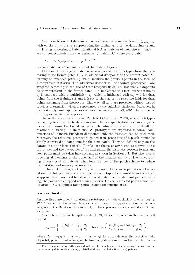
4.5 Processing of Very Large Dissimilarity Datasets 77
Assume as before that data are given as a dissimilarity matrix D = (dij)i,j=1,...,m
with entries dij = d(vi, vj) representing the dissimilarity of the datapoints vi andvj . During processing of Patch Relational NG, np patches of fixed size p = �m/np�are cut consecutively from the dissimilarity matrix D,3 where every patch
Pi = (dst)s,t=(i−1)·p+1,...,i·p ∈ �p×p
is a submatrix of D centered around the matrix diagonal.The idea of the original patch scheme is to add the prototypes from the pro-
cessing of the former patch Pi−1 as additional datapoints to the current patch Pi,forming an extended patch P ∗
i which includes the previous points in the form ofa compressed statistics. The additional datapoints – the former prototypes – areweighted according to the size of their receptive fields, i.e. how many datapointsdo they represent in the former patch. To implement this fact, every datapointvj is equipped with a multiplicity mj , which is initialized with mj = 1 for datapoints from the training set and it is set to the size of the receptive fields for datapoints stemming from prototypes. This way, all data are processed without loss ofprevious information which is represented by the sufficient statistics. Moreover, incontrast to dynamic approaches such as (Prudent and Ennaji, 2005) the number ofprototypes can be fixed a priori.
Unlike the situation of original Patch NG (Alex et al., 2009), where prototypescan simply be converted to datapoints and the inter-patch distances can always berecalculated using the Euclidean metric, the situation becomes more difficult forrelational clustering. In Relational NG prototypes are expressed as convex com-binations of unknown Euclidean datapoints, only the distances can be calculated.Moreover, the relational prototypes gained from processing of a patch cannot besimply converted to datapoints for the next patch. They are defined only on thedatapoints of the former patch. To calculate the necessary distances between theseprototypes and the datapoints of the next patch, the distances between former andnext patch must be taken into account, as shown in Section 4.3. But that meanstouching all elements of the upper half of the distance matrix at least once dur-ing processing of all patches, what foils the idea of the patch scheme to reducecomputation and memory-access costs.
In this contribution, another way is proposed. In between patches not the re-lational prototypes itselves but representative datapoints obtained from a so calledk-approximation are used to extend the next patch. As for standard patch cluster-ing, the points are equipped with multiplicities. On each extended patch a modifiedRelational NG is applied taking into account the multiplicities.
k-Approximation
Assume there are given n relational prototypes by their coefficient matrix (αij) ∈�n×m defined on Euclidean datapoints V . These prototypes are taken after con-vergence of the Relational NG method, i.e. these prototypes are situated at optimallocations.
As can be seen from the update rule (4.12), after convergence in the limit λ → 0it holds
αij −→{
1/|Ri| : vj ∈ Ri
0 : vj �∈ Ri, because
{hλ(kij) = 1 for vj ∈ Ri
hλ(kij) → 0 for vj �∈ Ri
},
where Ri = {vj ∈ V : ‖wi − vj‖ ≤ ‖wk − vj‖ for all k} denotes the receptive fieldof prototype wi. That means, in the limit only datapoints from the receptive fields
3The remainder is no further considered here for simplicity. In the practical implementationthe remaining datapoints are simply distributed over the first (M − p · np) patches.

78 Chapter 4 : Topographic Mapping of Dissimilarity Data
have positive coefficients and equally contribute to the winning prototype that islocated in the center of gravity of its receptive field.
A k-approximation of an optimal relational prototype wi is a subset R′ ⊆ Ri
with |R′| = min{k, |Ri|} such that∑
r′ ∈ R′ ‖wi−r′‖2 is minimized. That means, wechoose the k nearest points from the receptive field of a prototype as representatives.If there are less than k points in the receptive field, the whole field is taken. Thiscomputation can be done in time O(|Ri|·k). For a set W of relational prototypes, werefer to the set containing a k-approximation for each relational prototype wi ∈ Wa k-approximation of W .
These k-approximations in combination with their corresponding coefficients canbe interpreted as a convex-combined point in the relational model, defined just overthe points of the k-approximation. Therefore, if merged into the next patch, thenumber of the prototype coefficients remains limited, and the distances of theseapproximated prototypes to points of the next patch can be calculated using theoriginal equations. This way, only a fraction of the inter-patch distances needs tobe considered.
Construction of Extended Patches
Let Wt be a set of optimal relational prototypes gained in a step t. Assume Nt
denotes the index set of all points included in the union of a k-approximation ofWt pointing onto elements of the dissimilarity matrix D. The extended patch P ∗
t
is then characterized by the distance matrix
P ∗t =
⎛⎜⎜⎜⎜⎜⎜⎜⎜⎜⎜⎝
d(Nt−1) d(Nt−1, Pt)
d(Nt−1, Pt)T Pt
⎞⎟⎟⎟⎟⎟⎟⎟⎟⎟⎟⎠
where
d(Nt−1) = (duv)u,v ∈ Nt−1∈ �nt×nt
d(Nt−1, Pt) = (duv)u ∈ Nt−1,v=(t−1)·p+1,...,t·p ∈ �nt×p
denote the inter-distances of points from the k-approximation and the distancesbetween points from the k-approximation and current patch points, respectively.The size nt is bounded by |Wt| · k.
Integrating Multiplicities
The original Relational Neural Gas method has to be modified to handle data-points vj equipped with multiplicities mj . If these data points originate from ak-approximation of prototypes of the previous patch, the multiplicities are given by
m(wi) =1k·
∑v∈P∗
t ∩Vi(Wt)
m(v),
the sum of multiplicities of all data points in the receptive field divided by k.Incorporating multiplicities into the cost function yields the update rule
αij =mj · hλ(ki(vj))∑t mt · hλ(ki(vt))
for prototype coefficients. The computation of distances is not changed.

4.6 Experimental Results and Applications 79
Patch Relational Neural Gas
Assembling the pieces, we obtain Algorithm 4.5.
Algorithm 4.5: Patch Relational Neural Gas
Begin
Cut the first Patch P1
Apply Relational NG on P1 −→ Relational prototypes W1
Use k-Approximation on W1 −→ Index set N1
Update Multiplicities mj according to the receptive fields
Repeat for t = 2, . . . , np
Cut patch Pt
Construct Extended Patch P ∗t using Pt and index set Nt−1
Apply modified RNG with Multiplicities −→ Relational prototypes Wt
Use k-Approximation on Wt −→ Index set Nt
Update Multiplicities mj according to the receptive fields
Return k-approximation of final prototypes Nnp
End.
Complexity
Obviously, the size of extended patches is bounded by the size of the new patch readfrom the distance matrix and the distances of the at most k · n points representingthe n prototypes of the last run by their k approximation. Assume a boundedextended patch size p independent of the number of datapoints, as it would be thecase when the patch size is chosen according to memory limitations. The algorithmthen works only on O(m
p ·p2) = O(m ·p) = O(m) entries of the dissimilarity matrix,compared to O(m2) in the original RNG method. Moreover, the algorithm uses atmost O(p2) = const entries at a specific point in time.
In case of fixed patch size, also the time complexity is linear, because the RNGstep is O(p2) what results in O(p2 · m
p ) = O(p ·m) = O(m), an advantage comparedto the O(m2) time complexity of the original RNG. Furthermore, the algorithm canbe run in a single pass over the data.
These advantages in space and time complexity are obtained by an approxima-tion of the prototypes. As we will see in experiments, this leads only to a small lossin accuracy.Hence one of the key findings of this section is that the relational methods, despitetheir original quadratic time complexity, can now be applied successfully to the verylarge datasets arising in almost all fields of science today.
In the last section, we will focus on experiments and simulations that shalldemonstrate the benefits of the above presented methods on non-Euclidean datasets.
4.6 Experimental Results and Applications
In this section, we will demonstrate the benefits of the introduced methods onnon-Euclidean datasets.
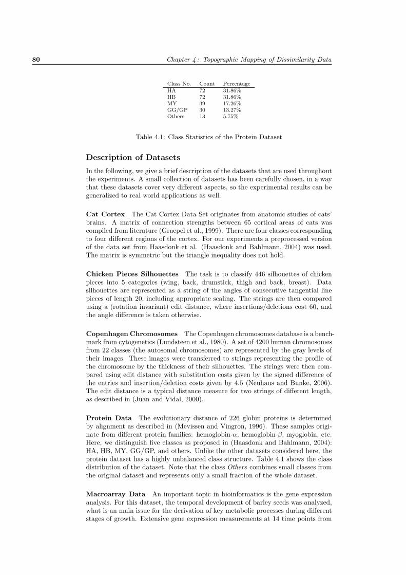
80 Chapter 4 : Topographic Mapping of Dissimilarity Data
Class No. Count PercentageHA 72 31.86%HB 72 31.86%MY 39 17.26%GG/GP 30 13.27%Others 13 5.75%
Table 4.1: Class Statistics of the Protein Dataset
Description of Datasets
In the following, we give a brief description of the datasets that are used throughoutthe experiments. A small collection of datasets has been carefully chosen, in a waythat these datasets cover very different aspects, so the experimental results can begeneralized to real-world applications as well.
Cat Cortex The Cat Cortex Data Set originates from anatomic studies of cats’brains. A matrix of connection strengths between 65 cortical areas of cats wascompiled from literature (Graepel et al., 1999). There are four classes correspondingto four different regions of the cortex. For our experiments a preprocessed versionof the data set from Haasdonk et al. (Haasdonk and Bahlmann, 2004) was used.The matrix is symmetric but the triangle inequality does not hold.
Chicken Pieces Silhouettes The task is to classify 446 silhouettes of chickenpieces into 5 categories (wing, back, drumstick, thigh and back, breast). Datasilhouettes are represented as a string of the angles of consecutive tangential linepieces of length 20, including appropriate scaling. The strings are then comparedusing a (rotation invariant) edit distance, where insertions/deletions cost 60, andthe angle difference is taken otherwise.
Copenhagen Chromosomes The Copenhagen chromosomes database is a bench-mark from cytogenetics (Lundsteen et al., 1980). A set of 4200 human chromosomesfrom 22 classes (the autosomal chromosomes) are represented by the gray levels oftheir images. These images were transferred to strings representing the profile ofthe chromosome by the thickness of their silhouettes. The strings were then com-pared using edit distance with substitution costs given by the signed difference ofthe entries and insertion/deletion costs given by 4.5 (Neuhaus and Bunke, 2006).The edit distance is a typical distance measure for two strings of different length,as described in (Juan and Vidal, 2000).
Protein Data The evolutionary distance of 226 globin proteins is determinedby alignment as described in (Mevissen and Vingron, 1996). These samples origi-nate from different protein families: hemoglobin-α, hemoglobin-β, myoglobin, etc.Here, we distinguish five classes as proposed in (Haasdonk and Bahlmann, 2004):HA, HB, MY, GG/GP, and others. Unlike the other datasets considered here, theprotein dataset has a highly unbalanced class structure. Table 4.1 shows the classdistribution of the dataset. Note that the class Others combines small classes fromthe original dataset and represents only a small fraction of the whole dataset.
Macroarray Data An important topic in bioinformatics is the gene expressionanalysis. For this dataset, the temporal development of barley seeds was analyzed,what is an main issue for the derivation of key metabolic processes during differentstages of growth. Extensive gene expression measurements at 14 time points from

4.6 Experimental Results and Applications 81
day zero after flowering to day 26 in steps of two days were carried out using cDNAmacroarray technology. High signal to noise ratios and high reproducibility betweentwo independently taken experimental series led to a selection of 4824 genes out of11786 genes available on the 12k macroarrays. Thus, a data matrix of 4824 (genes)by 14 (time points) is considered. As common in gene expression analysis, log2-transformed final expression values are considered. Coexpression analysis of theavailable 4824 gene expression time series is required to identify groups of commonlyregulated genes that may have temporal impact on each other. Such a clusteringhelps to extract candidate genes responsible for triggering later events like, forexample, the influence of cell wall degradation factors for lateral tissue nutrition orsubsequent starch accumulation processes.
Wisconsin Diagnostic Breast Cancer The Wisconsin Diagnostic Breast Can-cer database (WDBC) is a standard benchmark set from clinical proteomics (Wol-berg et al., 1995). This dataset is only Euclidean chosen to serve as benchmark.It consists of 569 Euclidean data points described by 30 real-valued input features:digitized images of a fine needle aspirate of breast mass are described by character-istics such as form and texture of the cell nuclei present in the image. The data arelabeled into two classes, benign and malignant.
Analysis of non-Euclidean Datasets
In the following the non-Euclidean datasets are analyzed regarding their Euclidean-ity. For that reason, characteristical properties like eigenvalues of the correspondingGram matrices are shown that have been discussed before in the last section.
The signatures of the dissimilarity matrices (inertia of corresponding Gram ma-trices) for the datasets is shown in Table 4.2. Except for the Protein dataset, alldissimilarity matrices feature a large value e− meaning there are many negativeeigenvalues in the spectra of the corresponding Gram matrices what indicates thatthey might be highly non-Euclidean.
Signature of Non-Euclidean Datasets
Cat Cortex (41,23,1)Chicken Pieces (240,205,1)Copenhagen Chromosomes (1951,2206,43)Macroarray Data (2450,2374,0)Protein Data (218,4,4)
Table 4.2: Inertia (e+, e−, e0) of corresponding Gram matrices
A more detailed view on the structure of the datasets is given by the magnitudeof the eigenvalues. Here, the non-Euclidean datasets used in the experiments areanalyzed by means of their sorted eigenspectra of the respective Gram matrices.The eigenvalues were normalized by the average dissimilarity before visualizationto make them more comparable.
As it can be seen, all datasets feature a few dominant positive eigenvalues andmany eigenvalues around zero, meaning that most structural information is con-tained only in a few dimensions. The negative eigenvalues are of a lower magnitudefor most datasets. It should be noted that the non-Euclidean part cannot be largerthan the Euclidean part, because the dissimilarities are constrained to be positive.

82 Chapter 4 : Topographic Mapping of Dissimilarity Data
Finally, we draw the reader’s attention to the Cat Cortex dataset (see Figure 4.3)which has a strong negative part in its eigenspectrum, so its non-Euclideanity ishigh.
0 10 20 30 40 50 60 70-2
-1
0
1
2
3
4
5
6
Figure 4.3: Cat Cortex Dataset: Eigenspectrum of Gram Matrix
0 50 100 150 200 250 300 350 400 450-20
0
20
40
60
80
100
120
140
Figure 4.4: Chicken Pieces Dataset: Eigenspectrum of Gram Matrix
Just to give an idea, Table 4.3 shows how large the spreading values have to bechosen to transform the dissimilarity into Euclidean or squared Euclidean distances,respectively.
Experimental Results on Dissimilarity Datasets
We demonstrate the performance of the relational algorithms in different scenariosgiven by the above described datasets covering a variety of characteristic situations.
Note that, for all median versions, prototypes situated at identical points ofthe data space do not separate in subsequent runs. Therefore constellations withexactly identical prototypes should be avoided. For the Euclidean and relationalversions this problem is negligible, presumed prototypes are initialized at differentpositions. However, for median versions it is likely that prototypes move to anidentical locations due to the limited number of different positions in data space,in particular for small data sets. To cope with this fact in median versions, we

4.6 Experimental Results and Applications 83
0 500 1000 1500 2000 2500 3000 3500 4000 4500-200
0
200
400
600
800
1000
1200
1400
1600
1800
Figure 4.5: Copenhagen Chromosome Dataset: Eigenspectrum of Gram Matrix
0 50 100 150 200 250-5
0
5
10
15
20
25
30
Figure 4.6: Protein Dataset: Eigenspectrum of Gram Matrix
add a small amount of noise to the distances in each epoch in order to separateidentical prototypes. In all runs, the methods have been applied directly withoutany correction of the given dissimilarity matrices.
For all experiments the initial neighborhood range λ0 is chosen as n/2 with n thenumber of neurons used. The neighborhood range λ(t) is decreased exponentiallywith the number of adaptation steps t according to λ(t) = λ0 · (0.01/λ0)t/tmax
(cf. (Martinetz et al., 1993)). The value tmax is chosen as the number of epochs.
Wisconsin Diagnostic Breast Cancer For training we used 40 neurons and150 epochs per run. The dataset was z-transformed beforehand. The results weregained from repeated 2-fold cross-validations averaged over 100 runs. The mixingparameter of the supervised methods was set to 0.5 for the simulations reported inTable 4.4. Moreover, the data set is contained in the Euclidean space therefore weare able to compare the relational versions introduced in this article to the standardEuclidean methods. These results are shown in Table 4.4. The effect of a variationof the mixing parameter is demonstrated in Fig. 4.7. The results are competitive tosupervised learning with the state-of-the-art-method GRLVQ as obtained in (Schleifet al., 2007).
As one can see, the results of Euclidean and relational clustering are identical, as

84 Chapter 4 : Topographic Mapping of Dissimilarity Data
Minimum Spread Transform
Dataset sq. Euclidean EuclideanCat Cortex 4.9321 (1.4105) 12.7616 (3.6495)Chicken Pieces 36.5429 (1.7107) 98.5631 (4.6142)Copenhagen Chromosomes 851.7972 (6.9389) 1865.9 (15.20)Macroarray Data 0.0028 (0.0031) 23.8977 (24.1545)Protein Data 0 (0) 12.6932 (1.2366)
Table 4.3: Minimum spreading value for the datasets to become squared Euclideanand Euclidean. In parentheses, the spreading value normalized by the averagedissimilarity is given.
k-Means Supervised Median Relational Supervisedk-Means k-Means k-Means Relational
k-Means
AccuracyMean 93.6 93.0 93.0 93.4 93.5StdDev 0.8 1.1 1.0 1.2 1.1
Batch Supervised Median Relational SupervisedNG Batch Batch Batch Relational
NG NG NG Batch NG
AccuracyMean 94.1 94.7 93.1 94.0 94.4StdDev 1.0 0.8 1.0 0.9 1.0
Table 4.4: Classification accuracy on the WDBC database for posterior labeling.The mean accuracy over 100 repeats of 2-fold cross-validation is reported.
expected by the theoretical background of relational clustering. Relational cluster-ing and supervision allow to improve the more restricted and unsupervised medianversions by more than 1% classification accuracy.
Cat Cortex The algorithms were tested in 10-fold cross-validation using 12 neu-rons (three per class) and 150 epochs per run. The results presented show themean accuracy over 250 repeated 10-fold cross-validations per method. The mixingparameter of the supervised methods was set to 0.5 for the simulations reported inTable 4.5. Results for different mixing parameters are shown in Figure 4.8.
Haasdonk and Bahlmann (2004) gained an accumulated error over all classesof at least 10% in leave-one-out experiments with SVMs. Graepel et al. (1999)obtained virtually the same results with the Optimal Hyperplane (OHC) algorithm.In our experiments, the improvement of restricted median clustering by relational
Median Median Relational Relational Supervised Supervised Supervisedk-Means Batch k-Means Batch Median Relational Relational
NG NG Batch NG k-Means Batch NG
AccuracyMean 72.8 71.6 89.0 88.7 77.9 89.2 91.3StdDev 3.9 4.0 3.3 3.0 3.5 3.0 2.8
Table 4.5: Classification accuracy on the Cat Cortex Data Set for posterior labeling.The mean accuracy over 250 repeats of 10-fold cross-validation is reported.

4.6 Experimental Results and Applications 85
0 0.1 0.2 0.3 0.4 0.5 0.6 0.7 0.8 0.90.93
0.935
0.94
0.945
0.95
0.955
0.96
Mixing Parameter
Mea
n A
ccur
acy
on T
est S
ets
Supervised Relational KMeansSupervised Median Batch NGSupervised Relational Batch NG
Figure 4.7: Results of the supervised methods for the WDBC data set with differentmixing parameters applied.
extensions by more than 10% classification accuracy can clearly be observed. Notethat relational clustering works quite well in this case although an interpretationby means of prototypes is not directly possible.
Proteins For training we used 45 neurons and 150 epochs per run. The resultswere gained from repeated 10-fold cross-validations averaged over 100 runs. Themixing parameter of the supervised methods was set to 0.5 for the simulationsreported in Table 4.6.
Unlike the results reported in (Haasdonk and Bahlmann, 2004) for SVM whichuses one-versus-rest encoding, the classification in our setting is given by only oneclustering model. Depending on the choice of the kernel, (Haasdonk and Bahlmann,2004) reports errors which approximately add up to 4% for the leave-one-out error.This result, however, is not comparable to our results due to the different errormeasure. A 1-nearest neighbor classifier yields an accuracy 91.6 for our setting (k-nearest neighbor for larger k is worse; (Haasdonk and Bahlmann, 2004)) which iscomparable to our results.
The Self-Organizing Map variants for dissimilarity datasets were tested againstthe Neural Gas variants. For training we use 29 neurons for Relational Batch NGand Relational Hyperbolic SOM, and a 5x5 grid for standard Relational SOM,respectively. The number of neurons is derived from the hyperbolic grid of depththree (cf. Figure 4.10). The neighborhood range is annealed starting from N/2 to
Median Median Relational Relational Supervised Supervised Supervisedk-Means Batch k-Means Batch Median Relational Relational
NG NG Batch NG k-Means Batch NG
AccuracyMean 76.1 76.3 88.0 89.9 89.4 88.2 90.0StdDev 1.3 1.8 1.8 1.3 1.4 1.7 1.0
Table 4.6: Classification accuracy on the Protein Data Set for posterior labeling

86 Chapter 4 : Topographic Mapping of Dissimilarity Data
0 0.1 0.2 0.3 0.4 0.5 0.6 0.7 0.8 0.90.7
0.75
0.8
0.85
0.9
0.95
Mixing Parameter
Mea
n A
ccur
acy
on T
est S
ets
Supervised Relational KMeansSupervised Median Batch NGSupervised Relational Batch NG
Figure 4.8: Results of the supervised methods for the Cat Cortex Data Set withdifferent mixing parameters applied.
0, N being the number of neurons, in all experiments. The results reported inTable 4.7 are gained from repeated 10-fold stratified cross-validation averaged over100 repetitions and 150 epochs per run. Supervision is included in the cost functionwith mixing parameter 0.5.
Note that the different clusters can easily be identified. The Relational SOMprovides an improved technique to explore dissimilarity data, revealing the struc-tures of interest.
The projections of a Relational SOM with hyperbolic grid structure and of Re-lational BNG with non-metric multidimensional scaling using Kruskal’s normalizedstress1 criterion are shown in figure 4.10 and 4.9. The neurons are depicted accord-ing to majority vote. Obviously, the neurons arrange according to the associatedclass and a very clear two-dimensional representation of the data set is obtained.
Copenhagen Chromosomes The Neural Gas variants for dissimilarity datasetswere tested in 2-fold stratified cross-validation using 100 neurons and 100 epochsper run (cf. (Cottrell et al., 2006)). The results presented are the mean accuracyover 10 times 2-fold cross-validation per method. The mixing parameter of thesupervised methods was set to 0.9.
As it can be seen from Table 4.8, supervised relational neural gas achieves anaccuracy of 0.914 for α = 0.9. This is an improvement by 8% compared to themedian variants.
Median Relational Standard RelationalBatch Batch Relational HyperbolicNG NG SOM SOM
Accuracy Protein Data setMean 89.5 92.4 91.5 91.5StdDev 1.0 0.9 0.8 1.2
Table 4.7: Classification accuracy on the Protein Data Set with posterior labeling
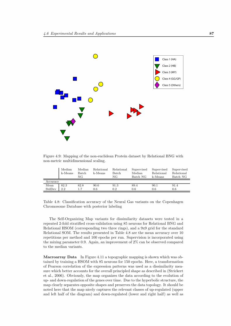
4.6 Experimental Results and Applications 87
Class 1 (HA)
Class 2 (HB)
Class 3 (MY)
Class 4 (GG/GP)
Class 5 (Others)
Figure 4.9: Mapping of the non-euclidean Protein dataset by Relational BNG withnon-metric multidimensional scaling.
Median Median Relational Relational Supervised Supervised Supervisedk-Means Batch k-Means Batch Median Relational Relational
NG NG Batch NG k-Means Batch NG
AccuracyMean 82.3 82.8 90.6 91.3 89.4 90.1 91.4StdDev 2.2 1.7 0.6 0.2 0.6 0.6 0.6
Table 4.8: Classification accuracy of the Neural Gas variants on the CopenhagenChromosome Database with posterior labeling
The Self-Organizing Map variants for dissimilarity datasets were tested in arepeated 2-fold stratified cross-validation using 85 neurons for Relational BNG andRelational HSOM (corresponding two three rings), and a 9x9 grid for the standardRelational SOM. The results presented in Table 4.8 are the mean accuracy over 10repetitions per method and 100 epochs per run. Supervision is incorporated usingthe mixing parameter 0.9. Again, an improvement of 2% can be observed comparedto the median variants.
Macroarray Data In Figure 4.11 a topographic mapping is shown which was ob-tained by training a HSOM with 85 neurons for 150 epochs. Here, a transformationof Pearson correlation of the expression patterns was used as a dissimilarity mea-sure which better accounts for the overall principled shape as described in (Strickertet al., 2006). Obviously, the map organizes the data according to the evolution ofup- and down-regulation of the genes over time. Due to the hyperbolic structure, themap clearly separates opposite shapes and preserves the data topology. It should benoted here that the map nicely captures the relevant classes of up-regulated (upperand left half of the diagram) and down-regulated (lower and right half) as well as

88 Chapter 4 : Topographic Mapping of Dissimilarity Data
Class 1 (HA)
Class 2 (HB)
Class 3 (MY)
Class 4 (GG/GP)
Class 5 (Others)
Figure 4.10: Mapping of the non-euclidean Protein dataset by a Relational SOMwith hyperbolic grid structure.
shapes in between.
Experimental Results on Magnification Control
We test local learning for a Euclidean benchmark, and four non-Euclidean settingsas described in (Neuhaus and Bunke, 2006; Haasdonk and Bahlmann, 2004). Inthe latter cases, local learning can be applied and it can be expected that ‘dense’or ‘sparse’ regions, respectively, of the data are emphasized depending on m dueto the optimized costs (4.17). However, the exact theoretical law of the prototypedensity and its information theoretic optimum is not known. Note that, if D�2
stems from a metric, the concept of dimensionality can be defined for the underly-ing data manifold and the intrinsic data dimensionality can been estimated using a
Median Relational Standard RelationalBatch Batch Relational HyperbolicNG NG SOM SOM
Accuracy Copenhagen Chromosome DatabaseMean 88.8 90.7 89.9 89.4StdDev 1.2 0.5 0.6 0.7
Table 4.9: Classification accuracy of the SOM variants on the Copenhagen Chro-mosome Database with posterior labeling

4.6 Experimental Results and Applications 89
Figure 4.11: Visualization of the macroarray dataset by Relational SOM with hy-perbolic grid structure.
Grassberger-Procaccia analysis (Grassberger and Procaccia, 1983). Similarly, den-sity estimation is possible for separable metric spaces and uniformly continuousdensities by means of histogram estimators (Geffroy, 1974). For simplicity, we com-pute P (v) using a simple Parzen window with bandwidth chosen as a third of theaverage point distance, which gives a rough approximation to the underlying densityfor Euclidean and metric settings, respectively.
For all experiments the initial neighborhood range λ0 was chosen as n/2, n beingthe number of neurons. The neighborhood range λ(t) at epoch t was decreasedaccording to λ(t) = λ0 · (0.01/λ0)t/tmax (cf. (Martinetz et al., 1993)), tmax being thenumber of epochs. If not indicated otherwise, the number of epochs was 100.
Control experiment At first, the experiment from (Hammer et al., 2007b) forEuclidean data was repeated for RNG as control. Data were sampled from thedistribution
(v1, . . . , vd,
d∏j=1
sin(π · vj))

90 Chapter 4 : Topographic Mapping of Dissimilarity Data
-1.5 -1 -0.5 0 0.5 1 1.5 2 2.5 3 3.53.84
3.85
3.86
3.87
3.88
3.89
3.9
3.91
m
Entr
opy
d = 1d = 2d = 3
-1.5 -1 -0.5 0 0.5 1 1.5 2 2.5 3 3.52.2
2.4
2.6
2.8
3
3.2
3.4
3.6
3.8
m
Entr
opy
Figure 4.12: Left: Euclidean benchmark data – Entropy of map formation for dif-ferent values c of magnification control and training sets of intrinsic dimensionalityd ∈ {1, 2, 3} — Right: Chicken Pieces Dataset – Entropy for different magnificationcontrol parameter values c
-1.5 -1 -0.5 0 0.5 1 1.5 2 2.5 3 3.5
3
3.1
3.2
3.3
3.4
3.5
3.6
3.7
m
Entr
opy
-1.5 -1 -0.5 0 0.5 1 1.5 2 2.5 3 3.50
0.1
0.2
0.3
0.4
0.5
0.6
0.7
0.8
0.9
1
m
True
Pos
itive
Rat
e
HAHBMYGG/GPOthers
Figure 4.13: Protein Dataset – Left: Entropy for different magnification controlparameter values c, Right: true positives rates
for d ∈ {1, 2, 3} and uniform vi ∈ [0, 1]. The number of data points was chosen as2500 for d = 1, 5000 for d = 2, and 10000 for d = 3. We trained RNG for controlvalues m ∈ [−1.5, 3.5] and step size 0.25. A NG network with 50 neurons has beenused. The reported results have been averaged over 20 runs.
The information theoretic quality of the map can be judged by computing thebalance of patterns in the receptive fields. For equal values, an optimum informationtransfer is achieved. The values of the map entropy are reported in Fig. 4.12. Theentropy should be maximum for optimum information transfer, i.e. for c = 2 (d = 1),c = 1 (d = 2), and c = 2/3 (d = 3). As indicated by the arrows, the experimentaloptima of the curves are closely situated to the expected theoretical values.
Protein Dataset For the experiment RNG with magnification control parameterc ∈ [−1.5, 3.5] (step size 0.1) and 50 neurons was trained. The results presented inFig. 4.13 are the average over 100 runs. The theoretical optimum c∗ ≈ 0.63 for theEuclidean case as indicated by the arrow in Fig. 4.13 was derived from the estimatedintrinsic dimension d ≈ 3.18. Note that magnification control by localized learningis obviously possible for this non-Euclidean setting. Interestingly, the informationtheoretic optimum of the curve is closely situated to the Euclidean one.
To demonstrate the magnification effect on exterior (small) classes, the truepositives rate for each class is depicted in Fig. 4.13. Apparently, the classificationrate is getting better when focusing on rare events, i.e. for small control parameterc.
Chicken Pieces Silhouettes Dataset We trained a RNG network with mag-nification control using 50 neurons and control parameter c ∈ [−1.5, 3.5] (step size

4.6 Experimental Results and Applications 91
-1.5 -1 -0.5 0 0.5 1 1.5 2 2.5 3 3.52
2.5
3
3.5
4
4.5
m
Entr
opy
-1.5 -1 -0.5 0 0.5 1 1.5 2 2.5 3 3.52.35
2.36
2.37
2.38
2.39
2.4
2.41
2.42
2.43
2.44
m
Entr
opy
Figure 4.14: Chromosome Dataset (left) and CatCortex Dataset (right) – Entropyfor different magnification control parameter values c
0.1). The average over 100 runs for each different value c was taken.The arrow in Fig. 4.13 indicates the theoretical optimum c∗ ≈ 0.54 for the
Euclidean case that was derived from the estimated intrinsic dimension d ≈ 3.72.
Copenhagen Chromosome Database Relational Neural Gas with magnifica-tion control has been trained using 80 neurons for control parameter c ∈ [−1.5, 3.5](step size 0.25).
The results shown in Fig. 4.14 present the average over 10 runs for each differentvalue c. The figure shows very smooth control of the map entropy by localized learn-ing. The observed optimum for the considered metric differs from the correspondingoptimum c∗ ≈ 0.68 (d ≈ 2.93) in the Euclidean case.
Cat Cortex Dataset For the experiment, Relational Neural Gas with magnifica-tion control has been trained using 12 neurons for control parameter c ∈ [−1.5, 3.5](step size 0.1). The results shown in Fig. 4.14 (right) present the average over 100runs. A Grassberger-Procaccia analysis cannot be applied due to the data statisticssuch that the theoretical optimum in the Euclidean case is not known. However,magnification control is clearly possible also in this case.
Experimental Results on Very Large Datasets
To show the overall performance of the proposed patch methods, we have chosensome representative very large dissimilarity datasets. Due to limited computingpower and hardware available, the chosen datasets do not represent real-life hugedatasets, they should be understood as a proof-of-concept that nevertheless caninstantly be transferred to the real problems.
We evaluate the clustering results by means of the classification error for su-pervised settings, whereby class labels are obtained by posterior labeling of proto-types. Note, however, that the goal of the algorithms is meaningful clustering ofdata based on a chosen similarity measure and cost function. Hence, the classi-fication error gives only a hint about the quality of the clustering, depending onwhether the class labels are compatible to the data clusters and chosen metric ornot. We accompany this supervised evaluation be the standard quantization errorof the clustering.
Synthetic Dataset To analyze the relation between the number of patches andthe quantization error on one hand, and the effect of k-approximation of relationalprototypes on the other hand, an artificial dataset from (Cottrell et al., 2006) wastaken. It consists of 1250 datapoints in the Euclidean plane gained from threeGaussian clusters.

92 Chapter 4 : Topographic Mapping of Dissimilarity Data
Effect of k-Approximation For an empirical study of the effect of k-approxima-tion on the quantization error, we trained 50 neurons with the original RelationalNG for 100 epochs, i.e. on average every neuron represents 25 datapoints. Onthe outcoming relational neurons, k-Approximation for k = 1, . . . , 20 were applied.Figure 4.15 shows a comparison of the quantization errors yielded with the differentapproximations to the quantization error gained by the original relational neurons.For each step the average over 10 runs is reported.
As expected, the quantization error decreases with higher numbers k of data-points used to approximate each relational neuron. Concerning the patch approach,applying a k-approximation to the relational neurons of each patch clearly resultsin a loss of accuracy depending on the choice of parameter k. But as can be seenlater on, even with k-approximation the quality of the results is still convincing.
2 4 6 8 10 12 14 16 18 2026
26.5
27
27.5
28
28.5
29
29.5
30
k
Qua
ntiz
atio
nE
rror
Relational NGk-Approximated RNG
Figure 4.15: Quantization error (i.e. E(W ) for λ → ∞) of original relational neuronscompared to different k-approximations on a synthetic dataset
Effect of Patch Sizes Analyzing the relation between the number of patcheschosen and the quantization error, we trained median and relational NG with 20neurons for 50 epochs. The results presented in figure 4.16 show the quantizationerror averaged over 10 runs for each number of patches. As expected, the quantiza-tion error increases with the number of patches used. But compared to the MedianPatch NG approach the presented Patch Relational NG performs very well withonly a small loss even for a larger number of patches used.
Chicken Pieces Silhouettes For training we used 30 neurons. For Patch Me-dian NG the dataset was divided into 4 patches, i.e. a patch size of around 111datapoints. The results reported in Table 4.10 are gained from a repeated 10-foldstratified crossvalidation averaged over 100 repetitions and 100 epochs per run. Thek-approximation for Patch Relational NG was done with k = 3.
Protein Classification The Protein Dataset as described on page 80 is processedby the patch variants of Neural Gas. For training we used 20 neurons. The datasetwas divided into 4 patches, i.e. a patch size of around 57 datapoints. The results
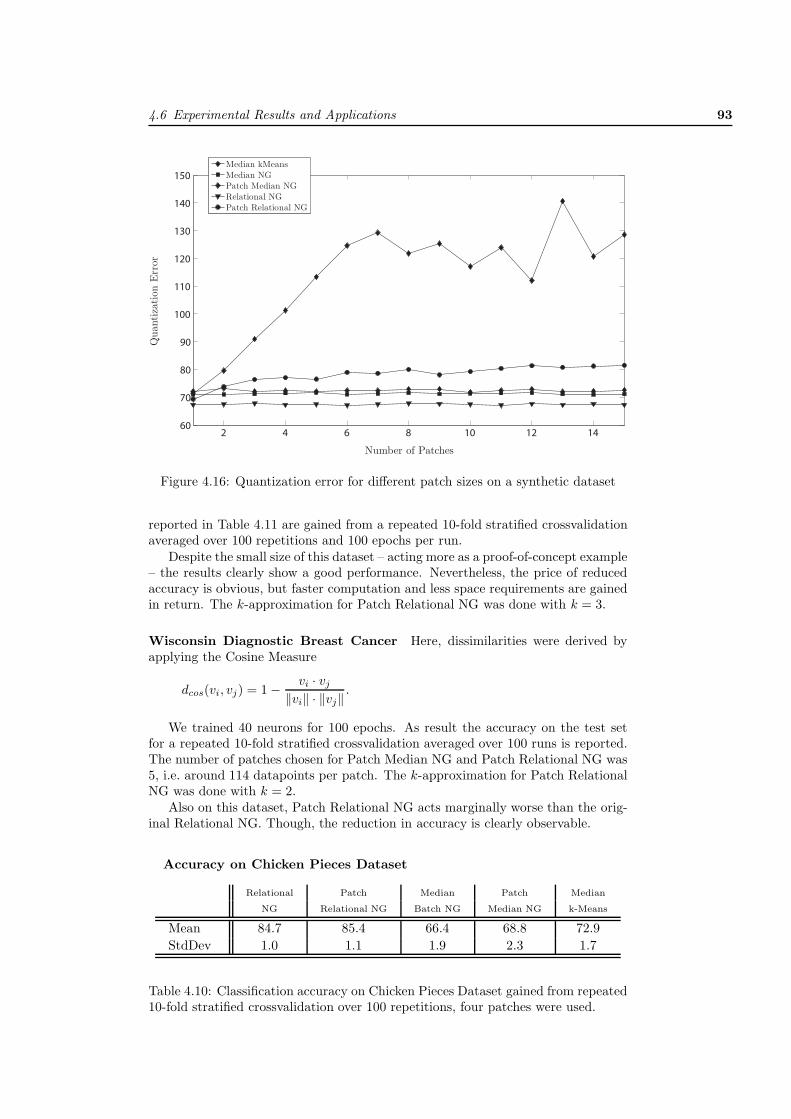
4.6 Experimental Results and Applications 93
2 4 6 8 10 12 1460
70
80
90
100
110
120
130
140
150
Number of Patches
Qua
ntiz
atio
nE
rror
Median kMeansMedian NGPatch Median NGRelational NGPatch Relational NG
Figure 4.16: Quantization error for different patch sizes on a synthetic dataset
reported in Table 4.11 are gained from a repeated 10-fold stratified crossvalidationaveraged over 100 repetitions and 100 epochs per run.
Despite the small size of this dataset – acting more as a proof-of-concept example– the results clearly show a good performance. Nevertheless, the price of reducedaccuracy is obvious, but faster computation and less space requirements are gainedin return. The k-approximation for Patch Relational NG was done with k = 3.
Wisconsin Diagnostic Breast Cancer Here, dissimilarities were derived byapplying the Cosine Measure
dcos(vi, vj) = 1 − vi · vj
‖vi‖ · ‖vj‖ .
We trained 40 neurons for 100 epochs. As result the accuracy on the test setfor a repeated 10-fold stratified crossvalidation averaged over 100 runs is reported.The number of patches chosen for Patch Median NG and Patch Relational NG was5, i.e. around 114 datapoints per patch. The k-approximation for Patch RelationalNG was done with k = 2.
Also on this dataset, Patch Relational NG acts marginally worse than the orig-inal Relational NG. Though, the reduction in accuracy is clearly observable.
Accuracy on Chicken Pieces Dataset
Relational Patch Median Patch Median
NG Relational NG Batch NG Median NG k-Means
Mean 84.7 85.4 66.4 68.8 72.9StdDev 1.0 1.1 1.9 2.3 1.7
Table 4.10: Classification accuracy on Chicken Pieces Dataset gained from repeated10-fold stratified crossvalidation over 100 repetitions, four patches were used.

94 Chapter 4 : Topographic Mapping of Dissimilarity Data
Copenhagen Chromosome Database The methods have been trained using60 neurons for 100 epochs. As result the accuracy on the test set for a repeated2-fold stratified crossvalidation averaged over 10 runs is reported. The number ofpatches chosen for Patch Median NG and Patch Relational NG was 10, i.e. around420 datapoints per patch. The k-approximation for Patch Relational NG was donewith k = 3.
Also on this dataset, Patch Relational NG acts well. Though, the reduction inaccuracy is clearly observable.
Experiments on Very Large Text Datasets
Here, the patch relational methods were applied to very large text datasets (Hasen-fuss et al., 2008a). For all text datasets, the extracted texts were pre-processedby removing stop words and applying word stemming (Porter, 1980). The textdocuments were then compared by the popular Normalized Compression Distance(NCD) (Cilibrasi and Vitani, 2005), a measure based on approximations of the Kol-mogorov Complexity from algorithmic information theory (Li and Vitanyi, 1997).The NCD is defined as
NCD(x, y) =C(xy) − min{C(x), C(y)}
max{C(x), C(y)}
where x and y are the document strings, C(x) denotes the compressed size of x andC(xy) the compressed size of the concatenation of x and y using a real compressor.For our experiments the bzip2 compression method was used.
Reuters Dataset The popular Reuters-21578 dataset is a collection of 21578documents that appeared on the Reuters newswire in 1987. The data was splitaccording to the common ’Modified Apte’ split and the most important class ofeach datapoint’s multilabel was taken as single class label. For the experiment the7 most prominent classes were taken (cf. Ontrup and Ritter, 2001). We traineda Supervised Patch Relational SOM with a hyperbolic grid of 85 neurons on 10patches for 100 epochs using a 5-approximation and a control parameter β = 0.5.Figure 4.17 shows the visualization as a simple projection of the hyperbolic gridinto the Euclidean plane.
20 Newsgroup Dataset The 20 Newsgroups dataset from the UCI repositoryconsists of 20000 newsgroup articles collected from twenty UseNet newsgroups dur-ing 1993, 1000 articles of each newsgroup. The newsgroups were grouped by theiroverall topics into 7 classes. We processed the data by a Supervised Patch Rela-tional SOM with a hyperbolic grid structure of 29 neurons on 60 patches. Training
Accuracy on Protein Dataset
Relational Patch Median Patch Median
NG Relational NG Batch NG Median NG k-Means
Mean 92.62 92.61 79.9 77.7 80.6StdDev 0.92 0.88 1.5 2.4 1.3
Table 4.11: Classification accuracy on Protein Dataset gained from repeated 10-foldstratified crossvalidation over 100 repetitions, four patches were used.
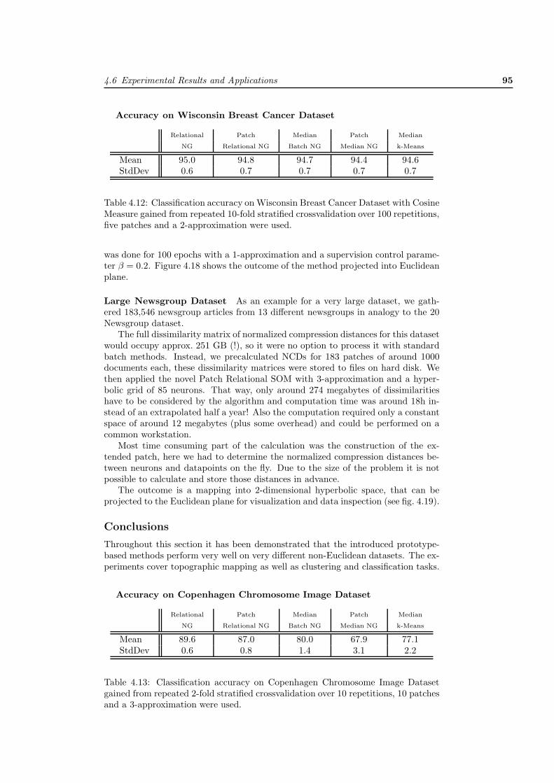
4.6 Experimental Results and Applications 95
Accuracy on Wisconsin Breast Cancer Dataset
Relational Patch Median Patch Median
NG Relational NG Batch NG Median NG k-Means
Mean 95.0 94.8 94.7 94.4 94.6StdDev 0.6 0.7 0.7 0.7 0.7
Table 4.12: Classification accuracy on Wisconsin Breast Cancer Dataset with CosineMeasure gained from repeated 10-fold stratified crossvalidation over 100 repetitions,five patches and a 2-approximation were used.
was done for 100 epochs with a 1-approximation and a supervision control parame-ter β = 0.2. Figure 4.18 shows the outcome of the method projected into Euclideanplane.
Large Newsgroup Dataset As an example for a very large dataset, we gath-ered 183,546 newsgroup articles from 13 different newsgroups in analogy to the 20Newsgroup dataset.
The full dissimilarity matrix of normalized compression distances for this datasetwould occupy approx. 251 GB (!), so it were no option to process it with standardbatch methods. Instead, we precalculated NCDs for 183 patches of around 1000documents each, these dissimilarity matrices were stored to files on hard disk. Wethen applied the novel Patch Relational SOM with 3-approximation and a hyper-bolic grid of 85 neurons. That way, only around 274 megabytes of dissimilaritieshave to be considered by the algorithm and computation time was around 18h in-stead of an extrapolated half a year! Also the computation required only a constantspace of around 12 megabytes (plus some overhead) and could be performed on acommon workstation.
Most time consuming part of the calculation was the construction of the ex-tended patch, here we had to determine the normalized compression distances be-tween neurons and datapoints on the fly. Due to the size of the problem it is notpossible to calculate and store those distances in advance.
The outcome is a mapping into 2-dimensional hyperbolic space, that can beprojected to the Euclidean plane for visualization and data inspection (see fig. 4.19).
Conclusions
Throughout this section it has been demonstrated that the introduced prototype-based methods perform very well on very different non-Euclidean datasets. The ex-periments cover topographic mapping as well as clustering and classification tasks.
Accuracy on Copenhagen Chromosome Image Dataset
Relational Patch Median Patch Median
NG Relational NG Batch NG Median NG k-Means
Mean 89.6 87.0 80.0 67.9 77.1StdDev 0.6 0.8 1.4 3.1 2.2
Table 4.13: Classification accuracy on Copenhagen Chromosome Image Datasetgained from repeated 2-fold stratified crossvalidation over 10 repetitions, 10 patchesand a 3-approximation were used.
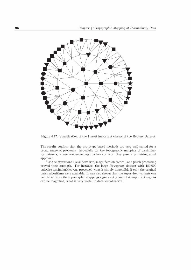
96 Chapter 4 : Topographic Mapping of Dissimilarity Data
Figure 4.17: Visualization of the 7 most important classes of the Reuters Dataset
The results confirm that the prototype-based methods are very well suited for abroad range of problems. Especially for the topographic mapping of dissimilar-ity datasets, where concurrent approaches are rare, they pose a promising novelapproach.
Also the extensions like supervision, magnification control, and patch processingproved their strength. For instance, the large Newsgroup dataset with 180,000pairwise dissimilarities was processed what is simply impossible if only the originalbatch algorithms were available. It was also shown that the supervised variants canhelp to improve the topographic mappings significantly, and that important regionscan be magnified, what is very useful in data visualization.

4.6 Experimental Results and Applications 97
Figure 4.18: Visualization of the UCI 20 Newsgroups Dataset

98 Chapter 4 : Topographic Mapping of Dissimilarity Data
Figure 4.19: Visualization of 183,546 newsgroup articles whose full dissimilaritymatrix would occupy approx. 251 GB, instead Patch Relation SOM was applied to183 patches of around 1000 documents each, reducing drastically the computationtime and space needed.

Chapter 5
Summary and Outlook
The concern of the thesis at hand was the processing of data for topographic map-ping as well as for clustering and classification. Throughout this work we wereexclusively concerned with prototype-based methods because these approaches of-fer very intuitive learning techniques and their outcomes are meaningful in a waythat they can be easily interpreted and visualized. We especially focused on thepopular prototype-based methods Neural Gas and Self-Organizing Maps, two rep-resentative approaches that have shown their benefits in many applications. NeuralGas is a very robust and reliable vector quantization technique that distributesrepresentative prototypes over a given data manifold in a topology-preserving way.Self-Organizing Maps are a very successful topographic mapping technique thatmap high-dimensional data into a low-dimensional structure where the data canbe visualized. Originally, these methods operate on vectorial data in Euclideanspaces. The ultimate goal of this thesis was the application of Neural Gas and Self-Organizing Maps to data given as pairwise dissimilarities between objects whichmeans in general that there is no vectorial representation available.
In the first part of the thesis, we reformulated the original standard methodsNeural Gas and Self-Organizing Maps to run in a so-called batch mode. In thismode, all the data points of a finite dataset are considered at once during eachupdate step of the algorithm. It could be demonstrated that the batch variantsachieve a higher order of convergence, i.e. they perform much faster while obtainingthe same outcome. These fast batch variants can always be used in place of theoriginal ones if the datasets are given in advance.
Next, a few useful extensions of Batch Neural Gas and Batch Self-OrganizingMaps were introduced. The first extension aimed for a better control on how theprototypes are distributed according to the data density. We discussed a modifi-cation of the update rules that allows for an arbitrary control of the magnificationbehaviour. This opened the way for outlier suppression, emphasis of rare events,and information optimal maps. In future work, the concept could also be extendedto user-interactive magnification of local regions, what would be particularly suitedfor sophisticated visualization tools in visual analytics.
If further information about the data in form of class labels is available, theadditional information can be incorporated into the learning process. It was shownthat this supervision helps to improve the classification ability as well as the qualityof the topographic maps for visualization.
Especially for the handling of very large datasets, we applied a special process-
99

100 Chapter 5 : Summary and Outlook
ing scheme that is based on patches. In principle this scheme can be applied to allprototype-based methods what is still subject of ongoing work. By taking patchesof fixed size one by one, this extension is able to process arbitrary large datasets.Beyond that, the scheme can also be applied to non-stationary distributions inthe context of life-long learning systems e.g. in pattern recognition for vision androbotics, or in clustering of data streams.
The main part of the thesis deals with the processing of dissimilarity datasetsthat are in general of non-Euclidean character. In particular, we adapted theprototype-based methods Neural Gas and Self-Organizing Maps to be able to workon non-vectorial datasets. In a first step, we introduced exemplar-based variantsthat use datapoints as representative prototypes. Unfortunately, the exemplar-based techniques feature the inherent drawback that the prototypes can only beplaced on fixed discrete locations what are in general suboptimal positions, partic-ularly if the data space is sparse. Therefore the main result of the thesis dealt witha further variant that overcomes those limitations.
How to do continuous updates in non-vectorial discrete spaces is not obvious atfirst feel. For that reason, we assumed an existing embedding into an Euclideanspace and introduced prototypes as convex combinations of data points. Based onthis assumption, we were able to derive update rules that only rely on the dissim-ilarities between data objects, and not on any vectorial representation. This ledstraightforward to Relational Neural Gas and Relational SOM which showed an ex-cellent performance on non-Euclidean dissimilarity datasets in the experiments. Wealso proposed extensions for magnification control and supervision. Furthermore,the patch scheme was adapted to the relational approach what rendered it possi-ble to generate prototype-based topographic mappings of very large dissimilaritydatasets that are far too large to compute all the pairwise dissimilaritites in ad-vance. To present viewable prototypes to the practitioner, the relational prototypescan be approximated by one or more nearest data points which are then presentedinstead as representatives.
All in all, the relational methods that were developed within this thesis arevery well suited for a broad range of applications in bioinformatics, experimentalphysics, web mining, robotics, and many other fields of science. Because of theirsimplicity, the practitioner only needs to define a dissimilarity measure for the dataobjects at hand and yet she has a collection of tools available providing her withintuitive prototype-based topographic mapping and clustering techniques. It shouldbe noted here that the crucial point in that process is the evaluation of the defineddissimilarity measures. This evaluation has to be done by experts in the field whocan be supported by proper visualizations of prototypes and data generated by therelational methods.
The research that was done in this thesis opens the way to interesting researchdirections. We would like to mention just a few:
Since the proposed relational methods showed excellent performance in practisealso on non-Euclidean datasets, it would be very interesting to accompany thealgorithms by a deeper mathematical investigation of their behaviour in pseudo-Euclidean spaces.
Obviously, for all relational methods the choice of an appropriate metric ordissimilarity measure is crucial for their performance. Since an optimum choice de-pends very much on the application at hand, it would be valuable to study whetheran adaptation of the metrics is possible in this framework. Alternatively, an al-

101
gorithm to pick an appropriate metric from a given finite set of metrics could befruitful, which could be based on general principles like clustering quality, for in-stance. Moreover, experts could be provided with a toolbox of metrics for commondata structures or application areas such as they are already partially available inbioinformatics. A combination of these three approaches in an interactive frame-work seems to be very promising for the next generation of data analysis tools.
As it was demonstrated, the patch paradigm constitutes an intuitive and effi-cient tool which turns standard prototype-based methods into an applicable modelfor huge datasets. Unfortunately, it seems that formal guarantees for the approxi-mation quality are difficult to obtain. Since the parameter k of the k-approximationis important for the quality of the results, heuristical approaches are imaginable toautomatically determine k such that a proper balance between accuracy and effi-ciency is obtained according to the application at hand. Also a variation of thepatch size over the course of learning seems to be useful, since more informationshould be preserved in earlier stages of the process. It has been demonstrated thatnon-stationary distributed incoming data can be handled using the patch scheme.Thus, the patch methods contribute not only to the processing of very large datasetsbut they also opens the way to life-long learning.
The methods developed within this thesis provide one of the rare linear prototype-based schemes for the processing of dissimilarity datasets which are suitable for dataanalysis in many different fields of science. To finally prove this claim it remainsto apply and evaluate the methods together with experts from different applicationfields. For this reason, the methods should be integrated into a toolbox that pro-vides nearly parameter free and robust access to the proposed algorithms for thepractitioners.

102 Chapter 5 : Summary and Outlook

Bibliography
N. Alex and B. Hammer. Parallelizing single patch pass clustering. In Proc. Euro-pean Symposium on Artificial Neural Networks (ESANN 2008), pages 227–232,2008.
N. Alex, A. Hasenfuss, and B. Hammer. Patch clustering for massive data sets.Neurocomputing, 72(7-9):1455–1469, 2009.
F. Aurenhammer. Voronoi diagrams - a study of a fundamental geometric datastructure. ACM Computing Surveys, 23(3):345–405, 1991.
F. R. Bach. Graph kernels between point clouds. In Proc. ICML ’08, pages 25–32.ACM, 2008.
H.-U. Bauer and K. Pawelzik. Quantifying the neighborhood preservation of self-organizing feature maps. IEEE Transactions on Neural Networks, 3(4):570–579,1992.
H.-U. Bauer and T. Villmann. Growing a hypercubical output space in a self-organizing feature map. IEEE Transactions on Neural Networks, 8:218–226, 1997.
H.-U. Bauer, M. Herrmann, and T. Villmann. Neural maps and topographic vectorquantization. Neural Networks, 12:659–676, 1999.
C. M. Bishop, M. Svensen, and C. K. I. Williams. Developments of the generativetopographic mapping. Neurocomputing, 21:203–224, 1998a.
C. M. Bishop, M. Svensen, and C. K. I. Williams. GTM: the generative topographicmapping. Neural Computation, 10(1):215–234, 1998b.
I. Borg and P. J. Groenen. Modern Multidimensional Scaling – Theory and Appli-cations. Springer, New York, 2005.
L. Bottou and Y. Bengio. Convergence properties of the kmeans algorithm. In Ad-vances in Neural Information Processing Systems, volume 7. MIT Press, Denver,1995.
R. Boulet, B. Jouve, F. Rossi, and N. Villa. Batch kernel SOM and related Laplacianmethods for social network analysis. Neurocomputing, 71(7–9):1257–1273, 2008.
P. Brucker. On the complexity of clustering algorithms. In R. Henn, B. Corte,and W. Oletti, editors, Optimierung und Operations Research – Lecture Notes inEconomics and Mathematical Systems, pages 44–55. Springer, 1978.
J. Bruske and G. Sommer. Dynamic cell structure learns perfectly topology pre-serving map. Neural Computation, 7(4):845–865, 1995.
K. Chang and J. Ghosh. A unified model for probabilistic principal surfaces. IEEETransactions on Pattern Analysis and Machine Intelligence, 23(1):22–41, 2001.
103

104 BIBLIOGRAPHY
K. Chang and J. Ghosh. Probabilistic principal surfaces. In Proc. IEEE Interna-tional Joint Conference on Neural Networks, 1999.
Y. Cheng. Convergence and ordering of Kohonen’s batch map. Neural Computation,9(8):1667–1676, 1997.
R. Cilibrasi and M. Vitani. Clustering by compression. IEEE Transactions onInformation Theory, 51(4):1523–1545, 2005.
J. C. Claussen and H. G. Schuster. Asymptotic level density of the elastic netself-organizing feature map. In ICANN ’02: Proceedings of the InternationalConference on Artificial Neural Networks, pages 939–944. Springer, 2002.
B. Conan-Guez, F. Rossi, and A. E. Golli. Fast algorithm and implementation ofdissimilarity self-organizing maps. Neural Networks, 19(6):855–863, 2006.
M. Cottrell, J. Fort, and G. Pages. Two or three things that we know about theKohonen algorithm. In Proc. European Symposium on Artificial Neural Networks(ESANN 1994), pages 235–244, 1994.
M. Cottrell, J. C. Fort, and G. Pages. Theoretical aspects of the SOM algorithm.In Neurocomputing, pages 119–138, 1998.
M. Cottrell, B. Hammer, A. Hasenfuß, and T. Villmann. Batch neural gas. InProceedings of the 5th Workshop on Self-Organizing Maps (WSOM 2005), pages275–282, 2005.
M. Cottrell, B. Hammer, A. Hasenfuß, and T. Villmann. Batch and median neuralgas. Neural Networks, 19:762–771, 2006.
R. Durbin and D. Willshaw. An analogue approach to the travelling salesmanproblem using an elastic net method. Nature, 326:689–691, 1987.
A. El Golli, B. Conan-Guez, and F. Rossi. A self organizing map for dissimilaritydata. In D. Banks, L. House, F. R. McMorris, P. Arabie, and W. Gaul, editors,Classification, Clustering, and Data Mining Applications (Proceedings of IFCS2004), pages 61–68, 2004.
E. Erwin, K. Obermayer, and K. Schulten. Self-organizing maps: ordering, conver-gence properties and energy functions. Biol. Cybern., 67:47–55, 1992.
F. Farnstrom, J. Lewis, and C. Elkan. Scalability for clustering algorithms revisited.SIGKDD Explorations, 2(1):51–57, 2000.
M. Filippone, F. Camastra, F. Masulli, and S. Rovetta. A survey of kernel andspectral methods for clustering. Pattern Recognition, 41(1):176–190, 2008.
J. Fort, P. Letremy, and M. Cottrell. Advantages and drawbacks of the batchkohonen algorithm. In Proc. European Symposium on Artificial Neural Networks(ESANN 2002), pages 223–230, 2002.
J.-C. Fort. SOM’s mathematics. Neural Networks, 19(6-7):812–816, 2006.
J.-C. Fort and G. Pages. On the a.s. convergence of the Kohonen algorithm with ageneral neighborhood function. Ann. Appl. Probab., 5(4):1177–1216, 1995.
J.-C. Fort and G. Pages. Quantization vs. organization in the Kohonen S.O.M. InProc. European Symposium on Artificial Neural Networks (ESANN 1996), pages85–89, 1996.

BIBLIOGRAPHY 105
A. Forti and G. L. Foresti. Growing hierarchical tree SOM: An unsupervised neuralnetwork with dynamic topology. Neural Networks, 19(10):1568–1580, 2006.
B. J. Frey and D. Dueck. Clustering by passing messages between data points.Science, 315:972–976, 2007.
B. Fritzke. A growing neural gas network learns topologies. In Advances in NeuralInformation Processing Systems 7, pages 625–632. MIT Press, 1995.
B. Fritzke. A self-organizing network that can follow non-stationary distributions.In W. Gerstner, A. Germond, M. Hasler, and J.-D. Nicoud, editors, ArtificialNeural Networks (ICANN 1997), volume 1327 of Lecture Notes in ComputerScience, pages 613–618, Berlin, 1997. Springer.
J. Geffroy. Sur l’estimation d’une densite dans un espace metrique.C.v.Acad.Sci.Paris Ser.A, 278:1449–1452, 1974.
A. Gersho and R. M. Gray. Vector Quantization and Signal Compression. KluwerAcademic Publishers, 1992.
I. Gohberg, P. Lancaster, and L. Rodman. Indefinite Linear Algebra and Applica-tions. Birkhauser, 2005.
L. Goldfarb. A unified approach to pattern recognition. Pattern Recognition, 17(5):575–582, 1984.
J. Gower and P. Legendre. Metric and euclidean properties of dissimilarity coeffi-cients. Journal of Classification, 3(1):5–48, 1986.
J. C. Gower. Some distance properties of latent root and vector methods used inmultivariate analysis. Biometrika, 53:325–338, 1966.
T. Graepel and K. Obermayer. A stochastic self-organizing map for proximity data.Neural Computation, 11(1):139–155, 1999.
T. Graepel, R. Herbrich, P. Bollmann-Sdorra, and K. Obermayer. Classification onpairwise proximity data. In Advances in neural information processing systems(NIPS), pages 438–444, 1999.
S. Graf and H. Luschgy. Foundations of Quantization for Probability Distributions.Springer, Berlin, 2000.
S. Graf and H. Luschgy. Rates of convergence for the empirical quantization error.Ann. Probab., 30(2):874–897, 2002.
P. Grassberger and I. Procaccia. Measuring the strangeness of strange attractors.Physica D, 9:189–208, 1983.
R. M. Gray and D. L. Neuhoff. Quantization. IEEE Transactions on InformationTheory, 44(6):2325–2383, 1998.
B. Haasdonk and C. Bahlmann. Learning with distance substitution kernels. In Pat-tern Recognition - Proc. of the 26th DAGM Symposium, volume 3175 of LectureNotes in Computer Science, pages 220–227, Berlin, 2004. Springer.
B. Hammer and A. Hasenfuss. Relational neural gas. In J. Hertzberg, M. Beetz, andR. Englert, editors, KI 2007: Advances in Artificial Intelligence, volume 4667 ofLecture Notes in Artificial Intelligence, pages 190–204, Berlin, 2007. Springer.

106 BIBLIOGRAPHY
B. Hammer and T. Villmann. Mathematical aspects of neural networks. In Proc.European Symposium on Artificial Neural Networks (ESANN 2003), pages 59–72,2003.
B. Hammer, M. Strickert, and T. Villmann. Supervised neural gas with generalsimilarity measure. Neural Processing Letters, 21:21–44, 2005.
B. Hammer, A. Hasenfuss, F.-M. Schleif, and T. Villmann. Supervised median clus-tering. In C. H. Dagli, editor, Smart Systems Engineering: Infra-Structure Sys-tems Engineering, Bio-Informatics and Computational Biology, and EvolutionaryComputation, Proceedings of the Artificial Neural Networks in Engineering Con-ference (ANNIE 2006), volume 16 of Intelligent Engineering Systems ThroughArtificial Neural Networks, pages 623–632, New York, 2006a. ASME Press. ISBN0-7918-0256-6.
B. Hammer, A. Hasenfuss, F.-M. Schleif, and T. Villmann. Supervised batch neu-ral gas. In F. Schwenker and S. Marinai, editors, Artificial Neural Networks inPattern Recognition, Second IAPR Workshop (ANNPR 2006), volume 4087 ofLecture Notes in Artificial Intelligence, pages 33–45, Berlin, 2006b. Springer.
B. Hammer, A. Hasenfuß, and T. Villmann. Magnification control for batch neuralgas. In Proceedings of the 14th European Symposium on Artificial Neural Networks(ESANN 2006), pages 7–12, 2006c.
B. Hammer, A. Hasenfuss, F. Rossi, and M. Strickert. Topographic processingof relational data. In Proceedings of the 6th International Workshop on Self-Organizing Maps (WSOM 2007), 2007a.
B. Hammer, A. Hasenfuss, and T. Villmann. Magnification control for batch neuralgas. Neurocomputing, 70(7–9):1225–1234, 2007b.
J. A. Hartigan and M. A. Wong. A K-means clustering algorithm. Applied Statistics,28:100–108, 1979.
A. Hasenfuss and B. Hammer. Relational topographic maps. In M. R. Berthold,J. Shawe-Taylor, and N. Lavrac, editors, Advances in Intelligent Data AnalysisVII, Proceedings of the 7th International Symposium on Intelligent Data Analysis(IDA 2007), volume 4723 of Lecture Notes in Computer Science, pages 93–105,Berlin, 2007. Springer.
A. Hasenfuss and B. Hammer. Single pass clustering and classification of largedissimilarity datasets. In Artificial Intelligence and Pattern Recognition (AIPR2008), pages 219–223, 2008.
A. Hasenfuss, B. Hammer, F.-M. Schleif, and T. Villmann. Neural gas clusteringfor dissimilarity data with continuous prototypes. In F. Sandoval, A. Prieto,J. Cabestany, and M. Grana, editors, Computational and Ambient Intelligence –Proceedings of 9th International Work-Conference on Artificial Neural Networks(IWANN 2007), volume 4507 of Lecture Notes in Computer Science, pages 539–546, Berlin, 2007. Springer.
A. Hasenfuss, W. Boerger, and B. Hammer. Topographic processing of very largetext datasets. In C. H. Dagli, editor, Smart Systems Engineering: ComputationalIntelligence in Architecting Engineering Systems (ANNIE 2006), volume 18 ofIntelligent Engineering Systems Through Artificial Neural Networks, pages 525–532, New York, 2008a. ASME Press.

BIBLIOGRAPHY 107
A. Hasenfuss, B. Hammer, T. Geweniger, and T. Villmann. Magnification control inrelational neural gas. In Proceedings of the 16th European Symposium on ArtificialNeural Networks (ESANN 2008), pages 325–330, 2008b.
A. Hasenfuss, B. Hammer, and F. Rossi. Patch relational neural gas - clusteringof huge dissimilarity datasets. In L. Prevost, S. Marinai, and F. Schwenker,editors, Artificial Neural Networks in Pattern Recognition, Third IAPR Workshop(ANNPR 2008), volume 5064 of Lecture Notes in Artificial Intelligence, pages 1–12, Berlin, 2008c. Springer.
T. Hastie. Principal Curves and Surfaces. PhD thesis, Stanford University, 1984.
T. Hastie and W. Stuetzle. Principal curves. Journal of the American StatisticalAssociation, 84:502–516, 1989.
R. J. Hathaway and J. C. Bezdek. Convergence of alternating optimization. Neural,Parallel Sci. Comput., 11(4):351–368, 2003.
R. J. Hathaway and J. C. Bezdek. Nerf c-means: Non-euclidean relational fuzzyclustering. Pattern Recognition, 27(3):429–437, 1994.
R. J. Hathaway, J. M. Huband, and J. C. Bezdek. Kernelized non-euclidean rela-tional fuzzy c-means algorithm. In The 14th IEEE International Conference onFuzzy Systems, pages 414–419, 2005.
T. Heskes. Transition times in self-organizing maps. Biological Cybernetics, 75(1):49–58, 1996.
T. Heskes. Energy functions for self-organizing maps. In E. Oja and S. Kaski,editors, Kohonen Maps, pages 303–315. Elsevier, Amsterdam, 1999.
T. Heskes and B. Kappen. Error potentials for self-organization. In IEEE Interna-tional Conference on Neural Networks, volume 3, pages 1219–1223, 1993.
H. Hirsh. Data mining research: Current status and future opportunities. StatisticalAnalysis and Data Mining, 1(2):104–107, 2008.
V. Hodge and J. Austin. A survey of outlier detection methodologies. ArtificialIntelligence Review, 22(2):85–126, 2004.
T. Hofmann and J. M. Buhmann. A theory of proximity based clustering: Structuredetection by optimization. Pattern Recognition, 33:617–634, 1999.
H. Hotelling. Analysis of a complex statistical variable into principal components.J. Educational Psychology, 24:417–441, 1933.
P. Indyk and J. Matousek. Low-distortion embeddings of finite metric spaces. InHandbook of Discrete and Computational Geometry, pages 177–196. CRC Press,2004.
E. T. Jaynes. Information theory and statistical mechanics. Physical Review, 106(4):620–630, 1957a.
E. T. Jaynes. Information theory and statistical mechanics ii. Physical Review, 108(2):171–190, 1957b.
I. Jolliffe. Principal Component Analysis. Springer, New York, 2002.
A. Juan and E. Vidal. On the use of normalized edit distances and an efficient k-nn search technique (k-aesa) for fast and accurate string classification. In ICPR2000, volume 2, pages 680–683, 2000.

108 BIBLIOGRAPHY
H. Kashima, K. Tsuda, and A. Inokuchi. Kernels for graphs. In B. Schoelkopf,K. Tsuda, and J. Vert, editors, Kernel Methods in Computational Biology, pages155–170. MIT Press, 2004.
S. Kaski, J. Kangas, and T. Kohonen. Bibliography of self-organizing map (SOM)papers: 1981-1997. Neural Computing Surveys, 1:102–350, 1998.
S. Kaski, J. Nikkila, M. Oja, J. Venna, P. Toronen, and E. Castren. Trustworthinessand metrics in visualizing similarity of gene expression. BMC Bioinformatics, 4(48), 2003.
S. Kaski, J. Nikkila, E. Savia, , and C. Roos. Discriminative clustering of yeaststress response. In U. Seiffert, L. Jain, and P. Schweizer, editors, Bioinformaticsusing Computational Intelligence Paradigms, pages 75–92. 2005.
D. A. Keim, F. Mansmann, D. Oelke, and H. Ziegler. Visual analytics: Combiningautomated discovery with interactive visualizations. In J.-F. Boulicaut, M. R.Berthold, and T. Horvath, editors, Discovery Science, volume 5255 of LectureNotes in Computer Science, pages 2–14. Springer, 2008.
T. Kohonen. Self-Organizing Maps. Springer, 2001.
T. Kohonen. Self-organized formation of topologically correct feature maps. Bio-logical Cybernetics, 43:59–69, 1982.
T. Kohonen and P. Somervuo. How to make large self-organizing maps for nonvec-torial data. Neural Networks, 15:945–952, 2002.
J. B. Kruskal. Multidimensional scaling by optimizing goodness of fit to a nonmetrichypothesis. Psychometrika, 29:1–27, 1964.
M. Li and P. Vitanyi. An Introduction to Kolmogorov Complexity and Its Applica-tions. Springer, 1997.
Y. Linde, A. Buzo, and R. Gray. An algorithm for vector quantizer design. IEEETransactions on Communications, 28:84–94, 1980.
R. Linsker. How to generate maps by maximizing the mutual information betweeninput and output signals. Neural Computation, 1:402–411, 1989.
S. P. Lloyd. Least squares quantization in PCM. IEEE Transactions on InformationTheory, 28(2):129–137, 1982.
H. Lodhi, C. Saunders, J. Shawe-Taylor, N. Cristianini, and C. Watkins. Textclassification using string kernels. Journal of Machine Learning Research, 2:419–444, 2002.
C. Lundsteen, J. Phillip, and E. Granum. Quantitative analysis of 6985 digitizedtrypsin G-banded human metaphase chromosomes. Clinical Genetics, 18:355–370,1980.
S. P. Luttrell. A Bayesian analysis of self-organizing maps. Neural Computation, 6(5):767–794, 1994.
D. MacDonald and C. Fyfe. The kernel self-organising map. In R. J. Howlett andL. C. Jain, editors, Proc. KES 2000, volume 4, pages 317–320. IEEE, 2000.
J. B. MacQueen. Some methods for classification and analysis of multivariate ob-servations. In Proc. 5th Berkeley Symposium on Mathematical Statistics andProbability, volume 1, pages 281–297, 1967.

BIBLIOGRAPHY 109
T. Martinetz and K. Schulten. Topology representing networks. Neural Networks,7(3):507–522, 1994.
T. Martinetz, S. Berkovich, and K. Schulten. ‘Neural gas’ network for vector quanti-zation and its application to time series prediction. IEEE Transactions on NeuralNetworks, 4(4):558–569, 1993.
J. Matousek. Lectures on Discrete Geometry. Springer, New York, 2002.
J. Matousek. Open problems on low-distortion embeddings of finite metric spaces.http://kam.mff.cuni.cz/∼matousek/metrop.ps, 2007.
E. Merenyi and A. Jain. Forbidden magnification? ii. In Proc. European Symposiumon Artificial Neural Networks (ESANN 2004), pages 57–62, 2004.
H. Mevissen and M. Vingron. Quantifying the local reliability of a sequence align-ment. Protein Engineering, 9:127–132, 1996.
C. Meyer. Matrix Analysis and Applied Linear Algebra. SIAM Society for Industrialand Applied Mathematics, Philadelphia, 2000.
B. Mokbel, A. Hasenfuss, and B. Hammer. Graph-based representation of symbolicmusical data. In A. Torsello, F. Escolano, and L. Brun, editors, Graph-BasedRepresentation in Pattern Recognition (GbRPR 2009), volume 5534 of LectureNotes in Computer Science, pages 42–51, Berlin, 2009. Springer.
F. Mulier and V. Cherkassky. Self-organization as an iterative kernel smoothingprocess. Neural Computation, 7(6):1165–1177, 1995.
M. Neuhaus and H. Bunke. Edit distance-based kernel functions for structuralpattern classification. Pattern Recognition, 39(10), 2006.
E. Oja. Oja learning rule. Scholarpedia, 3(3):3612, 2008.
E. Oja. A simplified neuron model as a principal component analyzer. Journal ofMathematical Biology, 15:267–273, 1982.
E. Oja. Principal components, minor components, and linear neural networks.Neural Networks, 5(6):927–935, 1992.
M. Oja, S. Kaski, and T. Kohonen. Bibliography of self-organizing map (SOM)papers: 1998-2001 addendum. Neural Computing Surveys, 3:1–156, 2003.
J. Ontrup and H. Ritter. Hyperbolic self-organizing maps for semantic navigation.In Advances in neural information processing systems 14 (NIPS), pages 1417–1424, 2001.
U. Ozertem. Locally Defined Principal Curves and Surfaces. PhD thesis, OregonHealth & Science University, 2008.
M. Parsana, S. Bhattacharya, C. Bhattacharya, and K. R. Ramakrishnan. Kernelson attributed pointsets with applications. In J. Platt, D. Koller, Y. Singer, andS. Roweis, editors, Advances in Neural Information Processing Systems 20, pages1129–1136. MIT Press, Cambridge, MA, 2008.
K. Pearson. On lines and planes of closest fit to systems of points in space. Philo-sophical Magazine, 2(6):559–572, 1901.
E. Pekalska and R. P. W. Duin. The Dissimilarity Representation for PatternRecognition. World Scientific Publishing, 2005.
110 BIBLIOGRAPHY
E. Pekalska, P. Paclik, and R. P. W. Duin. A generalized kernel approach todissimilarity-based classification. Journal of Machine Learning Research, 2:175–211, 2001.
M. Polla, T. Honkela, and T. Kohonen. Bibliography of self-organizing map (SOM)papers: 2002-2005 addendum. Neural Computing Surveys, 2007.
M. F. Porter. An algorithm for suffix stripping. Program, 14(3):130–137, 1980.
Y. Prudent and A. Ennaji. An incremental growing neural gas learns topology. InProc. IJCNN 2005, 2005.
A. K. Qinand and P. N. Suganthan. Kernel neural gas algorithms with applicationto cluster analysis. In Proc. ICPR 2004, volume 17(4), pages 617–620. IEEE,2004.
J. Qiu, M. Hue, A. Ben-Hur, J.-P. Vert, and W. S. Noble. A structural alignmentkernel for protein structures. Bioinformatics, 23(9):1090–1098, 2007.
B. Ripley. Pattern Recognition and Neural Networks. Cambridge, 1996.
H. Ritter. Self-organizing maps in non-euclidean spaces. In E. Oja and S. Kaski,editors, Kohonen Maps, pages 97–108. 1999.
H. Robbins and S. Monro. A stochastic approximation method. Annals of Mathe-matical Statistics, 22(3):400–407, 1951.
K. Rose. Deterministic annealing for clustering, compression, classification, re-gression, and related optimization problems. In Proceedings of the IEEE, pages2210–2239, 1998.
K. Rose, E. Gurewitz, and G. Fox. A deterministic annealing approach to clustering.Pattern Recognition Letters, 11(9):589–594, 1990.
K. Rose, E. Gurewitz, and G. Fox. Vector quantization by deterministic annealing.IEEE Transactions on Information Theory, 38(4):1249–1257, 1992.
F. Rossi. Model collisions in the dissimilarity SOM. In Proc. European Symposiumon Artificial Neural Networks (ESANN 2007), pages 25–30, 2007.
F. Rossi, A. Hasenfuß, and B. Hammer. Accelerating relational clustering algo-rithms with sparse prototype representation. In Proceedings of 6th InternationalWorkshop on Self-Organizing Maps (WSOM 2007), 2007.
V. Roth, J. Laub, M. Kawanabe, and J. M. Buhmann. Optimal cluster preserv-ing embedding of nonmetric proximity data. IEEE Trans. Pattern Analysis andMachine Intelligence, 25:2003, 2003.
J. Rynkiewicz. Self-organizing map algorithm and distortion measure. Neural Net-works, 19(6-7):830–837, 2006.
A. Saalbach, T. Twellmann, A. Wismuller, J. Ontrup, H. Ritter, and T. W. Nat-tkemper. A hyperbolic topographic mapping for proximity data. In Proc. ofthe IASTED International Conference on Artifical Intelligence and Applications,pages 106–111. ACTA Press, 2005.
A. A. Sadeghi. Convergence in distribution of the multi-dimensional kohonen algo-rithm. Journal of Applied Probability, 38(1):136–151, 2001.

BIBLIOGRAPHY 111
A. A. Sadeghi. Asymptotic behavior of self-organizing maps with nonuniform stimulidistribution. The Annals of Applied Probability, 8(1):281–299, 1998.
J. W. Sammon. A nonlinear mapping for data structure analysis. IEEE Trans.Comput., 18(5):401–409, 1969.
C. Saunders, J. Shawe-Taylor, and A. Vinokourov. String kernels, Fisher kernelsand finite state automata. In Advances in Neural Information Processing Systems15, pages 633–640. MIT Press, 2003.
V. Sauvage. The T-SOM (tree-SOM). In AI ’97: Proceedings of the 10th AustralianJoint Conference on Artificial Intelligence, pages 389–397, 1997.
F.-M. Schleif, B. Hammer, and T. Villmann. Margin based active learning for LVQnetworks. Neurocomputing, 70(7-9):1215–1224, 2007.
B. Scholkopf, A. Smola, and K.-R. Muller. Nonlinear component analysis as a kerneleigenvalue problem. Neural Computation, 10(5):1299–1319, 1998.
D. W. Scott. Multivariate Density Estimation: Theory, Practice, and Visualization.John Wiley & Sons, 1992.
J. Shawe-Taylor and N. Cristianini. Kernel Methods for Pattern Analysis. Cam-bridge University Press, 2004.
S. J. Simoff, M. H. Boehlen, and A. Mazeika, editors. Visual Data Mining – The-ory, Techniques and Tools for Visual Analytics, volume 4404 of Lecture Notes inComputer Science. Springer, 2008.
M. Strickert, U. Seiffert, N. Sreenivasulu, W. Weschke, T. Villmann, and B. Ham-mer. Generalized relevance LVQ (GRLVQ) with correlation measures for geneexpression analysis. Neurocomputing, 69:651–659, 2006.
H. Tong. Dimension Estimation and Models. World Scientific Publishing, 1993.
W. S. Torgerson. Multidimensional Scaling: I. Theory and Method. Psychometrika,17(4):401–419, 1952.
W. S. Torgerson. Theory & Methods of Scaling. Wiley, 1958.
J. Venna and S. Kaski. Local multidimensional scaling. Neural Networks, 19(6-7):889–899, 2006.
J. Vesanto, J. Himberg, E. Alhoniemi, and J. Parhankangas. SOM toolbox forMATLAB 5. Report A57, Helsinki University of Technology, April 2000.
N. Villa and F. Rossi. A comparison between dissimilarity SOM and kernel SOMfor clustering the vertices of a graph. In Proc. WSOM 2007, 2007.
T. Villmann. Controlling strategies for the magnification factor in the neural gasnetwork. Neural Network World, 10(4):739–750, 2000.
T. Villmann. Neural Maps and Learning Vector Quantization for Data Mining –Theory and Applications. Habilitationsschrift, University of Leipzig, 2004.
T. Villmann. Topologieerhaltung in selbstorganisierenden neuronalen Merkmal-skarten. Ph.d. thesis, University of Leipzig, 1997.
T. Villmann and J. C. Claussen. Magnification control in self-organizing maps andneural gas. Neural Computation, 18(2):446–469, 2006.

112 BIBLIOGRAPHY
T. Villmann and A. Heinze. Application of magnification control for the neuralgas network in a sensorimotor architecture for robot navigation. In H.-M. Gross,K. Debes, and H.-J. Bohme, editors, SOAVE 2000 – Selbstorganisation von adap-tivem Verhalten, pages 125–134. VDI-Verlag, 2000.
T. Villmann, R. Der, M. Herrmann, and T. Martinetz. Topology preservation in self-organizing feature maps: exact definition and measurement. IEEE Transactionson Neural Networks, 8(2):256–266, 1997.
T. Villmann, E. Merenyi, and B. Hammer. Neural maps in remote sensing imageanalysis. Neural Networks, 16(3-4):389–403, 2003.
T. Villmann, B. Hammer, F. Schleif, T. Geweniger, and W. Herrmann. Fuzzyclassification by fuzzy labeled neural gas. Neural Netw., 19(6):772–779, 2006.
C. von der Malsburg and D. J. Willshaw. How to label nerve cells so that theycan interconnect in an ordered fashion. Proceedings of the National Academy ofSciences of the United States of America, 74(11):5176–5178, 1977.
R. Weller. Inner sphere trees for proximity and penetration queries. Technicalreport, TU Clausthal, 2008.
D. J. Willshaw and C. von der Malsburg. How patterned neural connections can beset up by self-organization. Proceedings of the Royal Society of London. SeriesB, Biological Sciences, 194(1117):431–445, 1976.
T. Winkler, J. Drieseberg, A. Hasenfuss, B. Hammer, and K. Hormann. Thinningmesh animations. In O. Deussen, D. Keim, and D. Saupe, editors, Proceedings ofVision, Modeling, and Visualization (VMV 2008), 2008.
W. Wolberg, W. Street, D. Heisey, and O. Mangasarian. Computer-derived nuclearfeatures distinguish malignant from benign breast cytology. Human Pathology,26:792–796, 1995.
Q. Yang and X. Wu. 10 challenging problems in data mining research. InternationalJournal of Information Technology & Decision Making, 5(4):597–604, 2006.
G. Young and A. S. Householder. Discussion of a set of points in terms of theirmutual distances. Psychometrika, 3:19–21, 1938.
P. L. Zador. Development and Evaluation of Procedures for Quantizing MultivariateDistributions. Ph. D. Dissertation, Stanford University, 1963.
P. L. Zador. Asymptotic quantization error of continuous signals and the quan-tization dimension. IEEE Transactions on Information Theory, 28(2):139–148,1982.
Proximity — so close but still so far away. . .