topology and groupoids · a group. particular kinds of categories are the groupoids, of which in...
TRANSCRIPT

TOPOLOGY ANDGROUPOIDS:
A Geometric Account of General Topology,Homotopy Types and the Fundamental Groupoid
Ronald Brown, B.A., M.A., D.Phil., FLSW

This updated version first published in 2006 bywww.groupoids.org.uk
Deganwy, United Kingdom
Original version first published by McGraw-Hill in 1968 under the title Elements of
Modern Topology.
Second revised, updated and expanded version first published by Ellis Horwood
Limited in 1988 under the title Topology: A Geometric Account of General Topology,
Homotopy Types and the Fundamental Groupoid.
Version corrected January 20, 2020 by Taras Kolomatski
Printing and distribution by Createspaceavailable from amazon
c© 2006 R. Brown
COPYRIGHT NOTICEThis book is copyright. Subject to statutory exception, and the provision ofrelevant collective licensing arrangements, no reproduction may take placeof any part without the written permission of the author or his agents.
Contents
Preface to the first edition vii
Preface to the second edition x
Preface to the third edition xviii
1 Some topology on the real line 1
1.1 Neighbourhoods in R . . . . . . . . . . . . . . . . . . . . . . 1
1.2 Continuity . . . . . . . . . . . . . . . . . . . . . . . . . . . . 4
1.3 Open sets, closed sets, closure . . . . . . . . . . . . . . . . . 10
1.4 Some generalisations . . . . . . . . . . . . . . . . . . . . . . 14
2 Topological spaces 19
2.1 Axioms for neighbourhoods . . . . . . . . . . . . . . . . . . 20
2.2 Open sets . . . . . . . . . . . . . . . . . . . . . . . . . . . . 22
2.3 Product spaces . . . . . . . . . . . . . . . . . . . . . . . . . 27
2.4 Relative topologies and subspaces . . . . . . . . . . . . . . . 30
2.5 Continuity . . . . . . . . . . . . . . . . . . . . . . . . . . . . 33
2.6 Other conditions for continuity . . . . . . . . . . . . . . . . 38
2.7 Comparison of topologies, homeomorphism . . . . . . . . . 41
2.8 Metric spaces and normed vector spaces . . . . . . . . . . . 45
2.9 Distance from a subset . . . . . . . . . . . . . . . . . . . . . 57
iii

iv TOPOLOGY AND GROUPOIDS
2.10 Hausdorff spaces . . . . . . . . . . . . . . . . . . . . . . . . 59
3 Connected spaces, compact spaces 65
3.1 The sum of topological spaces . . . . . . . . . . . . . . . . . 65
3.2 Connected spaces . . . . . . . . . . . . . . . . . . . . . . . . 68
3.3 Components and locally connected spaces . . . . . . . . . . 72
3.4 Path-connectedness . . . . . . . . . . . . . . . . . . . . . . . 77
3.5 Compactness . . . . . . . . . . . . . . . . . . . . . . . . . . 82
3.6 Further properties of compactness . . . . . . . . . . . . . . 88
4 Identification spaces and cell complexes 97
4.1 Introduction . . . . . . . . . . . . . . . . . . . . . . . . . . . 97
4.2 Final topologies, identification topologies . . . . . . . . . . 101
4.3 Subspaces, products, and identification maps . . . . . . . . 105
4.4 Cells and spheres . . . . . . . . . . . . . . . . . . . . . . . . 113
4.5 Adjunction spaces . . . . . . . . . . . . . . . . . . . . . . . . 118
4.6 Properties of adjunction spaces . . . . . . . . . . . . . . . . 126
4.7 Cell complexes . . . . . . . . . . . . . . . . . . . . . . . . . 131
5 Projective and other spaces 141
5.1 Quaternions . . . . . . . . . . . . . . . . . . . . . . . . . . . 141
5.2 Normed vector spaces again . . . . . . . . . . . . . . . . . . 146
5.3 Projective spaces . . . . . . . . . . . . . . . . . . . . . . . . 147
5.4 Isometries of inner product spaces . . . . . . . . . . . . . . 152
5.5 Simplicial complexes . . . . . . . . . . . . . . . . . . . . . . 158
5.6 Bases and sub-bases for open sets; initial topologies . . . . . 162
5.7 Joins . . . . . . . . . . . . . . . . . . . . . . . . . . . . . . . 168
5.8 The smash product . . . . . . . . . . . . . . . . . . . . . . . 177
5.9 Spaces of functions, and the compact-open topology . . . . 181
CONTENTS v
6 The fundamental groupoid 201
6.1 Categories . . . . . . . . . . . . . . . . . . . . . . . . . . . . 202
6.2 Construction of the fundamental groupoid . . . . . . . . . . 207
6.3 Properties of groupoids . . . . . . . . . . . . . . . . . . . . . 215
6.4 Functors and morphisms of groupoids . . . . . . . . . . . . 219
6.5 Homotopies . . . . . . . . . . . . . . . . . . . . . . . . . . . 225
6.6 Coproducts and pushouts . . . . . . . . . . . . . . . . . . . 234
6.7 The fundamental groupoid of a union of spaces . . . . . . . 240
7 Cofibrations 253
7.1 The track groupoid . . . . . . . . . . . . . . . . . . . . . . . 254
7.2 Fibrations of groupoids . . . . . . . . . . . . . . . . . . . . . 262
7.3 Examples . . . . . . . . . . . . . . . . . . . . . . . . . . . . 278
7.4 The gluing theorem for homotopy equivalences of closed
unions . . . . . . . . . . . . . . . . . . . . . . . . . . . . . . 284
7.5 The homotopy type of adjunction spaces . . . . . . . . . . . 291
7.6 The cellular approximation theorem . . . . . . . . . . . . . 304
8 Some combinatorial groupoid theory 313
8.1 Universal morphisms . . . . . . . . . . . . . . . . . . . . . . 314
8.2 Free groupoids . . . . . . . . . . . . . . . . . . . . . . . . . 325
8.3 Quotient groupoids . . . . . . . . . . . . . . . . . . . . . . . 331
8.4 Some computations . . . . . . . . . . . . . . . . . . . . . . . 334
9 Computation of the fundamental groupoid 341
9.1 The Van Kampen theorem for adjunction spaces . . . . . . . 341
9.2 The Jordan Curve Theorem . . . . . . . . . . . . . . . . . . 354
10 Covering spaces, covering groupoids 361
10.1 Covering maps and covering homotopies . . . . . . . . . . . 362
10.2 Covering groupoids . . . . . . . . . . . . . . . . . . . . . . . 367
10.3 On lifting sums and morphisms . . . . . . . . . . . . . . . . 371

vi TOPOLOGY AND GROUPOIDS
10.4 Existence of covering groupoids . . . . . . . . . . . . . . . . 375
10.5 Lifted topologies . . . . . . . . . . . . . . . . . . . . . . . . 381
10.6 The equivalence of categories . . . . . . . . . . . . . . . . . 389
10.7 Induced coverings and pullbacks . . . . . . . . . . . . . . . 395
10.8 Applications to subgroup theorems in group theory . . . . . 401
11 Orbit spaces, orbit groupoids 411
11.1 Groups acting on spaces . . . . . . . . . . . . . . . . . . . . 411
11.2 Groups acting on groupoids . . . . . . . . . . . . . . . . . . 417
11.3 General normal subgroupoids and quotient groupoids . . . . 421
11.4 The semidirect product groupoid . . . . . . . . . . . . . . . 425
11.5 Semidirect product and orbit groupoids . . . . . . . . . . . 428
11.6 Full subgroupoids of orbit groupoids . . . . . . . . . . . . . 433
12 Conclusion 439
A Functions, cardinality, universal properties 445
A.1 Functions . . . . . . . . . . . . . . . . . . . . . . . . . . . . 445
A.2 Finite, countable and uncountable sets . . . . . . . . . . . . 450
A.3 Products and the axiom of choice . . . . . . . . . . . . . . . 456
A.4 Universal properties . . . . . . . . . . . . . . . . . . . . . . 459
Glossary of terms from set theory 467
Bibliography 472
Glossary of symbols 495
Index 501

Preface to the first edition
This book is intended as a textbook on point set and algebraic topologyat the undergraduate and immediate post-graduate levels. In particular,I have tried to make the point set topology commence in an elementarymanner suitable for the student beginning to study the subject.
The choice of topics given here is perhaps unusual, but has the aim ofpresenting the subject with a geometric flavour and with a coherent out-look. The first consideration has led to the omission of a number of topicsimportant more from the point of view of analysis, such as uniform spaces,convergence, and various alternative kinds of compactness. The secondconsideration, together with restriction of space, has led to the omission ofhomology theory, of the theory of manifolds, and of any complete accountof simplicial complexes. It has also led to the omission of topics which areimportant but not exactly germane to this book; for example, I have not in-cluded accounts of paracompactness or the theory of continua, nor proofsof the Tychonoff theorem or the Tietze extension theorem.
I felt, on the other hand, that the general direction of this book shouldbe towards homotopy theory, since this subject links naturally with thepoint set topology and also occupies a central role in modern developments.However, in homotopy theory there are a number of ideas and construc-tions which are important in many applications (particularly the ideas ofadjunction space, cell complex, join, and homotopy extension property)but for which no elementary account has appeared. One of my aims, then,has been to cover this sort of topic, and so to supplement existing accounts,rather than provide a new reference book to contain everything a younggeometer ought to know. At the same time, I have tried to show that pointset topology has its main value as a language for doing ‘continuous geome-try’; I believe it is important that the subject be presented to the student inthis way, rather than as a self-contained system of axioms, definitions, andtheorems which are to be studied for their own sake, or for their interesta generalisations of facts about Euclidean space. For this reason, I havekept the point set topology to the minimum needed for later purposes, and
vii

viii TOPOLOGY AND GROUPOIDS
at the same time emphasised general processes of construction which leadto interesting topological spaces, and for which other structures, such asmetrics or uniformities, are largely irrelevant.
The language of point set topology is geometric. On the other hand,the notions of category and functor are algebraic: they play in modernmathematics the unifying role which has earlier been given to the notion ofa group. Particular kinds of categories are the groupoids, of which in turngroups are special cases. The algebra of groupoids has been developedrecently by P. J. Higgins. In 1965, I discovered the utility of this algebra forcomputing the fundamental group, and this has led me to include in thelast four chapters of this book an account of the elements of the algebra ofcategories and groupoids. The treatment given in these chapters is quitenovel, in that this algebra is used in an essential way and not just as aconvenient, but not entirely necessary, general language. The writing ofthese chapters gave me great pleasure as I found the way in which thevarious topological nations of sum, adjunction space, homotopy, coveringspace, are modelled by the corresponding notions for groupoids. The mostimportant feature here is probably the way in which the computations ofthe fundamental group derive from a general property of the fundamentalgroupoid (that it sends ‘nice’ pushouts to pushouts). This contrasts withthe usual rather ad hoc computation via simplicial complexes.
The development of these last four chapters has meant that I have hadto cut down on some other topics. For example, I have had to relegatethe accounts of k-spaces, infinite cell complexes, and function spaces tothe Exercises. A further reason for playing down these topics was that therecent development of the theory of quasi-topological spaces is likely tolead to a radical change in their exposition (cf. [Spa63] and a forthcomingbook by Dyer and Eilenberg). I have also relegated to the Exercises thediscussion of group-like structures and exact sequences, and have omittedan account of the major properties of the Whitehead product. The reasonsbehind this were lack of space, the difficulty of presenting computations,and, finally, the feeling that these topics needed reconsideration in the lightof the preceding work on groupoids.
The material in this book would more than cover a two-term under-graduate course in point set and algebraic topology. Such a course couldinclude, for the point set topology, all of chapters 1 to 3 and some ma-terial from chapters 4 and 5. This could be followed by a course on thefundamental groupoid comprising chapter 6 and parts of chapters 8 or 9;naturally, more could be covered if this were linked with a course on cate-gories and functors.
The last four chapters, with supporting parts of chapters 4 and 5, wouldprobably be suitable for a two-term M.Sc. course. Alternatively, the purely

PREFACE TO THE FIRST EDITION ix
algebraic parts of the last four chapters would cover the elements (but withnot enough algebraic applications) of a one-term course on groupoids.
The Appendix contains an account of functions, cardinality, and some‘universal constructions’ which are used from chapter 4 onwards. On pages467 to 471 (of this edition) is a Glossary of those terms from set theorywhich are used in the book but not defined in the main text.
This book is not self-contained—in particular, it will be assumed at cer-tain points that the reader is familiar with the usual accounts of vectorspaces and of groups.
On the other hand, a more ‘topological’ account of elementary analysisis by no means universal. For this reason, and in order to motivate theaxioms for a topological space, I have started the book with an account ofthe elementary topological notions on the real line R.
In the earlier chapters, I have included among the exercises a fair num-ber of straightforward verifications or simple tests of the reader’s under-standing. Apart from a few simple definitions and verifications, no resultsfrom the exercises are used in the text; this means that occasionally a re-sult from an exercise is actually proved later in the text. However, there aresome cross-references among the exercises themselves. Exercises from laterchapters are usually more difficult than those from earlier ones—exercisesof technical difficulty are marked with an asterisk.
Cross-references are always given in square brackets; thus [6.5.12]refers to 5.12 of §5 of chapter 6. The end of a Proof is denoted by thesymbol �.
I would like to thank Dr W. F. Newns for reading through much of themanuscript and for many suggestions which resulted in improved exposi-tion and in the removal of errors. I would also like to thank Professor G.Horrocks and Dr R. M. F. Moss for their comments on some of the chapters.I am indebted to Dr P. J. Higgins for conversations and letters; for sendingme notes of a course on groupoids he gave at King’s College, London in1965; and for writing his paper, [Hig63].
I would also like to thank Dr W. Gilbert, P. R. Heath, D. Pitt, T. Poston,Dr E. Rees, and E. E. Thompson for help in proofreading.
RONALD BROWN
Hull, 1968

x TOPOLOGY AND GROUPOIDS

Preface to the second
edition
When the first edition of this book ended its print-run in 1972, I did nottake up the publisher’s offer to reprint it with corrections, owing to an ideathat I could improve on the book in some key aspects of organisation. Thisidea turned out to be a misconception.
It is true that one particular criticism had some justice, namely the feel-ing that there was a jump in level of abstraction at chapter 6, which in-troduces the idea of category. Thus there was the possibility of making atwo-volume work, with maybe more complete material in each. The dif-ficulty was the close cross-links, in substance and in spirit, between thetwo parts. So the present edition makes no attempt to change the originalglobal conception.
A further difficulty in making major changes was that the original manu-script had been written with a vision and energy which by the mid-1970shad turned into a research programme arising out of the work on groupoidswhich had gone into the text. In particular, the notion of higher homotopygroupoids and higher dimensional Van Kampen theorems began to takeshape with the help of colleagues and research students, and I found itimpossible to take up the task of reshaping the text.
However, a good deal of the material in the book is still unavailableelsewhere. Also, the categorical spirit in which the book was written,and in particular the use of universal properties, has not penetrated manyother books in topology at this level. This is quite surprising in view ofthe comment in W. S. Massey’s excellent 1967 book on algebraic topology([Mas67]): ‘This method of characterising various mathematical structuresas solutions to universal mapping problems seems to be one of the truly uni-fying mathematical principles to have emerged since 1945, and it should bebrought into the mathematics curriculum as early as possible.’ For exam-ples of the use of universal properties in computer science, see the articles
xi

xii TOPOLOGY AND GROUPOIDS
in [PAPR86], which is the proceedings of a conference on category theoryand computer programming.
A further surprise to me has been that twenty years after the publica-tion of the first edition the theory of the fundamental groupoid still is nottaken by many topologists as a necessary and convenient generalisation ofthe theory of the fundamental group. Thus no other English language texton topology in print has followed the exposition given here. It thereforeseemed essential to make this exposition available for a judgement to bepossible on the convenience or elegance of this approach. Also much hashappened since the previous edition was published, so that it is now pos-sible to put the methods more in context, and to add extra applications.There is a new section on the Jordan Curve Theorem in which the proofuses the Van Kampen theorem for non-connected spaces in an essentialway. There are mew section on covering morphisms of groupoids, and newsections on the fundamental groupoid, and hence on the fundamental gr-oup, of an orbit space. The notion of fibration of groupoid is used in anessential way.
The exposition given here lends credence to the view that groupoidsform a natural context for discussing a key question in mathematics, therelation between local and global phenomena. This idea is confirmed inthe area of differential geometry by the following quotation from the intro-duction to [Mac87]:
‘The concept of groupoid is one of the means by which the twen-tieth century reclaims the original domain of applications of thegroup concept. The modern rigorous concept of group is far toorestrictive for the range of geometrical applications envisagedin the work of Lie. There have thus arisen the concepts of Liepseudogroup, of differentiable and Lie groupoid, and of prin-cipal bundle—as well as various related infinitesimal conceptssuch as Lie equation, graded Lie algebra and Lie algebroid—by which mathematics seeks to acquire a rigorous language bywhich to study the geometric phenomena associated with geo-metrical transformations which are only locally defined.’
It thus seems that the notion of groupoid gives a more flexible and pow-erful approach to the notion of symmetry.
I will be pleased if the exposition of this book can be improved in radicalways. Young mathematicians should be aware of the temporary mature ofmathematical exposition. The attempt to form a ‘final view’ reminds one ofthe schoolboy question: what would happen if you laid worms in a straightline from Marble Arch to Picadilly Circus? Answer: one of them would bebound to wiggle and spoil it all.

PREFACE TO THE SECOND EDITION xiii
Some might argue that the groupoid worm has here not only wiggledfrom its accustomed place in topology, but become altogether too big forits boots, to which a worm, after all, has no rights. But I hope many willfind it interesting to trace through this first attempt to answer, in part, thequestions: Is it possible to rewrite homotopy theory, substituting the wordgroupoid for the word group, and making other consequential changes? Ifthis is done, is the result more pleasing?
These questions, both of the form ‘What if. . . ?’, came to acquire for mea force and an obsession when pursued into the topic of higher homotopygroupoids. The scribbling of countless squares and cubes and their compo-sitions lead to a conviction in 1966 that the standard group theory, once itwas rephrased as a groupoid theory, had a generalisation to higher dimen-sions. Gradually, collaborations with Chris Spencer in 1971–1974, withPhilip Higgins since 1974, with J.-L. Loday from 1981, and work of myresearch students, A. Razak Salleh, Keith Dakin, Nick Ashley, David Jones,Graham Ellis and Ghaffar Mosa, at Bangor, and Philip Higgins’ research stu-dents Jim Howie and John Taylor at London and Durham, made the theorytake shape. In this way a worry of the algebraic topologists of the 1930sas to why the higher homotopy group were abelian, and so less compli-cated than the fundamental group, came to seem a genuine question. Thesurprising answer is that the higher homotopy groupoids are non-abelian,and are just right for doing many aspects of homotopy theory. In particular,they satisfy a version of the Van Kampen theorem which enables explicitand direct computations to be made. It will be interesting to see if thehigher dimensional theory will come to bear a relation to the standard gr-oup theory similar to that of many-variable to one-variable calculus.
But the higher dimensional theory is a story in which we cannot embarkin this book. We now give the changes that have been made in this newedition.
A section on function spaces in the category of k-spaces has been addedthe chapter 5. One of the reasons is that the material is quite difficult tofind elsewhere. Another reason for its inclusion is that it will suggest to thereader that there are still matters to be decided on the appropriate settingfor our intuitive notions of continuity. In any case, the generalisation fromspaces to k-spaces makes the proofs if anything simpler.
I am grateful to a number of people for comments, particularly EldonDyer and Peter May who suggested that chapter 7 needed clarification,and Daniel Grayson who suggested the notation [(X, i), (Y,u)] now used inchapter 7 to replace the original X//u, which was non-standard and toobrief. (But this double slash is used in a new context in chapter 9.) Inthe event, chapter 7 has been completely revised to make use of the termcofibration rather than HEP. The idea of fibration of groupoid, which came

xiv TOPOLOGY AND GROUPOIDS
to light towards the end of the writing of the first edition and so appearedthere only in an exercise, has now been incorporated into the main text.However, I have not included fibrations of spaces, since to do so wouldhave enlarged the text unduly, or force the omission of material for whichno other textbook account is available.
In chapter 8, an error in section 8.2 has been corrected. Also freegroupoids have now been used to define the notion of path in a graph.An exercise on the computation of the fundamental group of a union ofnon-connected spaces has now been incorporated into the text, as an illus-tration of the methods and because of its intrinsic importance. This resultis used in a new section which gives a proof of the Jordan Curve Theorem,and some new results on the Phragmen-Brouwer Property.
In chapter 9, section 9.4 on the existence of covering groupoids hasbeen rewritten to give a clearer idea of the notion of action of groupoidson sets. Section 9.5 includes some results on topologising the fundamen-tal groupoid. The relation between covering spaces of X and coveringgroupoids of πX has been clarified by adding section 9.6, which gives an ac-count of the equivalence of the categories of these objects. This enables analgebraic account of the theory of regular covering spaces. Section 9.7 givesa new account of pullbacks of covering spaces and covering morphisms, us-ing exact sequences. Section 9.8 gives an account of the Nielsen-Schreierand Kurosch subgroup theorems, using groupoid versions, due to Hasseand Higgins, of the more traditional covering space proofs.
Sections 9.9 to 9.10 give the first account in any text of the theoryof the fundamental groupoid of an orbit space. This uses work of JohnTaylor an Philip Higgins, and is a good illustration of the utility of thegroupoid methods, since a group version is considerably more awkward inthe statement of results and in the proofs. I am grateful to Ross Geogheganwho, in a review of a paper by M. A. Armstrong, pointed out the desirabilityof having Armstrong’s results on the computation of the fundamental groupof an orbit space available in a text.
The Bibliography has been extended for this edition. It would be im-possible to make such a Bibliography complete, and I apologise in advancefor any omissions or lack of balance. The main intention has been to showthe subject matter of this book as part of a wide mathematical scene; occa-sionally it is used to give the reader an opportunity to explore some aspectswhich are not so well represented in texts; other times, the Bibliographyis used to acknowledge clear debts. The Notes at the ends of chapters,and referential material in the text have the aim of giving an impressionof what the subject is about, of how mathematics is an activity involvingpeople, and that it is a subject in a state of active development, even in itsfoundations.

PREFACE TO THE SECOND EDITION xv
I would like to thank the following for helpful comments and criticisms:Philip Higgins, Alan Pears, Guy Hirsch, Peter May, Terry Wall, Frank Adams,Jim Dugundji, R. E. Mosher. I also thank all those who wrote and pointedout misprints and obscurities.
I would like to conclude this preface on a personal note, which I hopemay be of use to readers starting on, or aspiring to, a career in mathe-matical research, and wondering what that might entail. There is little inprint on the methodology of mathematical research. There is material onproblem solving, but there is little on evaluation, on problem choice, or onproblem and concept formulation. There is material on the psychology ofinvention, but not so much on the training and development of invention,nor so much on the ends to which one should harness whatever inventionone has. There are autobiographies available, but some perhaps give theimpression that to do research in mathematics it is helpful to be a genius inthe first place.
At the time of writing the first edition of this book, I was not clear asto what direction I wanted to take in my research, and to some extentwriting the book was a displacement activity, distracting attention fromthe necessity of decision. However, as the book progressed and I tried tomake the exposition clear, difficulties in the subject began to emerge. Asdraft succeeded draft, I became clearer about what I did not know, anda new range of possibilities began to arise. The original intention was astandard exposition of known, but scattered, material. This turned into anidiosyncratic treatment which itself suggested a new research line whichhas kept me busy ever since.
So I would like to commend to readers the idea that writing and rewrit-ing mathematics with an intention to make things clear, well organised andcomprehensible, and perhaps with some particular formal changes in mind,may in itself be a stimulus to further mathematical activity. These ideas areconfirmed by some remarks of the composer Maurice Ravel, who arguedfor copying from other composers. If you have something to contribute,then this will appear of itself, and if you have no new ideas in this area,then at the least you will have made things clear to yourself. Thus the qual-ity of your understanding is improved. There is also the simple joy of awell-crafted work.
There is also an argument for the quality of misunderstanding. It maybe easy for you to feel that you do not understand because you are stupid.But your lack of understanding may be a reaction to a lack of clarity inthe current expositions, or a feeling that the current expositions requiresomething more to carry conviction. These expositions may prove results,but not explain them in a way you find agreeable. The only way to tell is totry and write an account for yourself, and see if you can make the matter

xvi TOPOLOGY AND GROUPOIDS
clearer. For example, the material on the gluing theorem in chapter 7 wasmy response to a lack of understanding of the complicated proofs in theliterature of results such as 7.5.3 (Corollary 2). By the time of the finaldraft, I was clear why these results were true.
The account of groupoids which has dominated both editions of thisbook came about in the following way. It was annoying to have a Van Kam-pen theorem which did not compute the fundamental group of a circle. Ifound that the account of the Van Kampen theorem given by [Olu58] couldbe generalised to yield this computation (see [Bro64]). So I started an ex-position of Olum’s non-abelian cohomology, with the laudable motivationthat this would also introduce cohomological ideas to the reader. Unfortu-nately, when I looked at the 30 pages of my draft, I had to admit that theywere pretty boring.
At the same period I had been pursuing some references on free groups.These lead me to the article [Hig63], which introduced free products withamalgamation of groupoids. So it seemed reasonable to set an exercise onthe fundamental groupoid π(U ∪ V) of a union of spaces. Since the resultwas not in the literature as such, it seemed reasonable to write out a solu-tion. The solution turned out to have the qualities of elegance, concisionand clarity which I had been hoping for, but had not obtained, in my pre-vious account. This suggested that the exposition should be turned roundto give groupoids a central rather than peripheral role, particularly in viewof a warm reception to a seminar I gave on the topic to the London Alge-bra Seminar in 1965. In 1967, I met Professor G. W. Mackey of HarvardUniversity who told me of his work using groupoids in ergodic theory. Thissuggested that the groupoid concept had a wider application than I hadenvisaged, and so I also worked up chapter 9 on covering spaces, empha-sising the groupoid viewpoint. It is perhaps only now possible to see themany disparate strands of work in which the notion of groupoid is usefullyinvolved (cf. the survey article [Bro87]).
I would like to acknowledge here the help of two people who startedme on a mathematical career. I have a great debt to the late Professor J.H. C. Whitehead, who was patient with my hesitancies and confusions. Hismany successes in exposing the formalities underlying geometric phenom-ena are a background to this text, and one part of my aims was to givean exposition of his lemmas on the homotopy type of adjunction spaces.From him I also absorbed the attitude of not giving up a mathematical ideauntil its essentials had been extracted, whatever the apparent relevance orotherwise to current fashions.
My second debt is to Professor M. G. Barratt, who initiated me intothe practicalities and impracticalities of mathematical research. As to theimpracticalities, I once got a ten-page letter from him which ended: ‘Dawn

PREFACE TO THE SECOND EDITION xvii
breaks; I hope nothing else does!’ As to the practicalities, I remember think-ing to myself after a long session with Michael: ‘If Michael Barratt can tryout one damn fool thing after another, why can’t I?’ This has seemed areasonable way of proceeding ever since. What is not so clear is why thereally foolish projects (such as higher homotopy groupoids, based on flimsyevidence, and counter to current traditions) have turned out the most fun.
My thanks also go to Ellis Horwood and his staff. The production of thisnew edition has been greatly assisted by their expertise and enthusiasm.
RONALD BROWN
March, 1988

xviii TOPOLOGY AND GROUPOIDS

Preface to the third edition
The second edition of this book went out of print in 1994 or so, partlydue to the publisher Ellis Horwood Ltd being sold. The final impetus fora new version came with funding from a Leverhulme Emeritus Fellowship,2002–2004.
Background to the approach in this bookThe republishing of this text is intended to make available material un-
available in other texts. The retitling of the book and some chapters isintended to show a major emphasis of this and previous editions: the mod-
elling of geometry, principally topology, by the algebra of groupoids. The waythis modelling works illustrates some important general principles, whichare worth explaining.
The process of understanding some geometry may, over many years, gothrough the stages
geometry // underlyingprocesses
// algebra // algorithms // computation
each of which has its own interest, character and problems. The algebragives a precise, but possibly not total, expression of what we envision as theunderlying processes. The end product, some computations, will hopefullygive some specific answers to geometrical questions. The computationsmay be by hand, or if sufficiently complex, in a computer implementa-tion. The success of the computations in answering geometrical questions‘proves’ the methodology, in the old sense of ‘prove’ as ‘test’.
In choosing algebra to model geometry there is a tendency to take thealgebraic structures which are to hand—groups, rings, fields, and so on—but a certain eclecticism is necessary, and one should allow the geometry,an intuition for the underlying processes, and a feeling for mathematicalstructures, to formulate the algebra so that it expresses our intuitions. Ex-perience shows that in this way understanding and modes of computationare increased. Possibly more importantly, we may in this way find new
xix
xx TOPOLOGY AND GROUPOIDS
forms of algebra, algorithms and modes of computation, of general signifi-cance. In this way, mathematics develops language for description, verifica-tion, deduction and calculation, and that is a major reason for its necessityin science and technology.
This book shows the use of groupoids for this aim and in this context ofbasic algebraic topology.
The chief difference between groupoids and groups is that in groupoidsthere is a partial multiplication which is defined under geometric condi-tions: two arrows compose if and only if the end point of one is the initialpoint of the other. The arrows a,b in the diagram
xa−→ y
b−→ z
‘compose’ to give an arrow ba : x→ z. This corresponds to the compositionof journeys. Conversely, the analysis of a journey through various placesrequires precisely this notion of partial composition. So, to express our in-tuitions, we are, if we so allow ourselves, forced into considering groupoidsrather than just groups. The theory of groupoids has added to group theorya spatial component, coming from the geography of the places we visit in ajourney. For this reason, groupoids can model more of the geometry thangroups alone. This leads not only to more powerful theorems with simplerand more natural proofs, but also to new theorems and new landscapes.
The process of modelling needs more explanation. We prove that thefundamental groupoid takes certain constructions on spaces to analogousconstructions on groupoids. The use of analogy is fundamental to math-ematics, though not always acknowledged publicly. When we note that2+3 = 3+2 and 2×3 = 3×2 are examples of the commutative law, we aremaking an analogy between addition and multiplication of numbers. Wethen note that the commutative law applies to many situations, for examplealso to the addition of vectors. But numbers are not analogous to vectors,so how does this analogy come about? This seems to be an anomaly.
We mentioned above an analogy between certain constructions onspaces and constructions on groupoids. Yet spaces are very different fromgroupoids: they are different types of mathematical structure, withoutmany analogies between the way they are defined. How can we makeanalogies between constructions on them?
The answer is a very important principle. In mathematics, and in manyareas, analogies are not between objects themselves, but between the re-lations between objects. We will define many constructions by their rela-tions to all other objects of the same type—this is called a ‘universal prop-erty’. A certain construction on topological spaces which we call ‘pushout’is defined by its relation to all topological spaces; a certain construction

PREFACE TO THE THIRD EDITION xxi
on groupoids which we also call ‘pushout’ is defined by its relation to allgroupoids. Further, relations between topological spaces are given by thecontinuous functions between them. Relations between groupoids are de-fined by the morphisms between groupoids. Once the term pushout is de-fined in each context, the analogy between the two definitions will be com-pletely clear. However the construction of a pushout in spaces is necessarilydifferent in detail from the construction of a pushout of groupoids. Thuswithout the universal properties, the analogy might not be seen. All this isthe essence of the ‘categorical approach’, and explains why category theory,which we use explicitly or implicitly, has been a major unifying force in themathematics of the 20th century.
As an instance, the fact that the fundamental group of the circle is aninfinite cyclic group is seen as an analogy between the following two dia-grams (which are both pushouts!)
{0, 1}
��
// {0}
��[0, 1] // S1
spaces
{0, 1}
��
// {0}
��I // Z
groupoids
The left hand diagram shows the circle as obtained from the unit interval[0, 1] by identifying, in the category of spaces, the two end points 0, 1. Theright hand diagram shows the infinite group of integers as obtained fromthe finite groupoid I, again by identifying 0, 1, but this time in the categoryof groupoids. The right hand diagram is not available for groups.
The groupoid I with its special arrow ι : 0 → 1 has the following prop-erty: if g is an arrow of a groupoid G then there is a unique morphismg : I → G whose value on ι is g. Thus the groupoid I with ι plays forgroupoids the same role as does for groups the infinite cyclic group Z withthe element 1: they are each free on one generator in their respective cat-egory. However we can draw a complete diagram of the elements of I asfollows:
0::
ι))1
ι−1
ii dd
whereas we cannot draw a complete picture of the elements of Z.The analogy between the above pushouts of spaces and groupoids gen-
eralises to the analogy between a space Y obtained from a space X by iden-tifying various points of a discrete subspace, and a groupoid H obtained

xxii TOPOLOGY AND GROUPOIDS
from a groupoid G by identifying various objects of G. The necessary alge-bra of groupoids for this is developed in Chapter 8, and the relation withtopology in Chapter 9.
A necessary background to this method of universal properties is the no-tion of a category, which we give in Chapter 6, developing just that amountof theory needed for our results. We also develop some simple set theoreticexamples of universal properties in the Appendix.
Other analogies we make are in Chapter 10, between covering maps ofspaces, and covering morphisms of groupoids; and in Chapter 11, betweenorbit spaces under the action of a group, and orbit groupoids under theaction of a group. Here also we prove the main result by verifying the re-quired universal property of an orbit groupoid, and go on to examine waysof constructing and calculating orbit groupoids. This approach is not onlyeasier to follow and more efficient, but also can suggest wider possibilitiesfor investigation.
The types of problems in this book which we translate from topology toalgebra using groupoids come largely under the heading of local-to-global
problems. These problems are an important feature of mathematics andscience. Much of algebraic topology is about methods for solving suchproblems. The distinctive nature of the fundamental group in these meth-ods of algebraic topology is that it gives a nonabelian invariant, and theuse of groupoids gives an extra power to this aspect. This power is alsoshown by the increasing use of groupoids in many fields of mathematicsand physics, partly through allowing not only a more flexible approach tosymmetry than groups alone, but also allowing for an algebra correspond-ing to transitions. Forms of multiple groupoids yield higher dimensionalnonabelian methods for local-to-global problems.
With regard to the index, we take the line as in previous editions that itis better to be over- rather under-indexed, so that the index can possibly actas a guide, particularly in the e-version, with hyperref. Thus ‘topologicalgroup’ appears in the index under ‘topological’ and under ‘group’. We mayhave failed on this principle in a number of instances, for which apologiesin advance.
The changes for this edition are modest but significant.
1) We have already mentioned the retitling of the book and some chapters,and there has been a division of each the previous last two chapters intotwo, in order to give a clearer structure to the content.
2) Corrections have been made where known and found, and the diagramshave been improved where possible.
Finally, even if this is obvious to you, we must mention a major socialchange in freedom of mathematics information since the last edition ofthis book, namely the use since the 1980s of TEX and LATEX, and of course

PREFACE TO THE THIRD EDITION xxiii
the growth of the Internet. These together have led in mathematics to:free electronic journals; free independent Internet encyclopaedias; searchengines; the notion of e-book; the preprint arXiv; and many others. Thismeans that a reader with access to the Internet can follow up and evaluatetopics and concepts in a way not dreamt of in the 1980s. Hence if you wantto follow up any reference to wider reading given in this book, you are welladvised also to check out for yourself using Internet resources.
Acknowledgements
I have been greatly helped by a number of organisations and people.
The Leverhulme Foundation awarded me a Leverhulme Emeritus Fel-lowship for 2002–2004, part of whose aim was to publish this new edition.This book will also be a foundation for a book again supported in thatperiod by the Fellowship, authored with Philip Higgins and Rafael Sivera,entitled Nonabelian algebraic topology. It will include an exposition of workof the author and Philip Higgins over the period 1974–2005 on applica-tions of crossed complexes and related higher order groupoids in algebraictopology and the cohomology of groups.
Booksurge LLC have the organisation which makes this book readilyavailable, in terms of printing and price.
La Monte Yarrol made a first draft of the LATEX for the whole book in1994. Peilang Wu revised this draft in 2003, and Gareth Evans has re-vised and overseen the final production version, during 2005-6. They bothgreatly improved the diagrams.
John Robinson and Ben Dickins designed the cover. For more informa-tion on the origin of the sculpture ‘Journey’, see www.popmath.org.uk.
I have been fortunate in many happy collaborations on the ‘groupoidproject’.
Philip Higgins introduced me to groupoids. This resulted in a long col-laboration, fully employing his algebraic mastery and expository skills. His1971 book ‘Categories and groupoids’, which overlaps this one, is availableas a downloadable reprint.
Jean-Louis Loday showed how to take nonabelian methods in a newdirection, yielding in particular a nonabelian tensor product of groups withhomotopical and algebraic applications.
Jean Pradines and Kirill Mackenzie introduced me to Lie groupoids.
Tim Porter and Chris Wensley at Bangor have helped me enormouslyover the years: Tim particularly in algebraic and categorical background,and Chris in computational methods. Many research students have ven-tured into this groupoid territory, made important contributions and oftenbecame collaborators: Phil Heath (Hull), Lew Hardy, Tony Seda, RazakSalleh, Keith Dakin, Nick Ashley, Andy Tonks, Ghafar Mosa, Fahd Al-Agl,

xxiv TOPOLOGY AND GROUPOIDS
Osman Mucuk, Ilhan Icen, Anne Heyworth, Emma Moore.I also thank Alexander Grothendieck for an exuberant correspondence
in the years 1982–1991: he described this as a baton rompu, which roughlymeans ‘ranging over this and that’, and indeed it dealt with many mattersof mathematics and life.
RONALD BROWN
Deganwy, January 2006

Does the pursuit of truth give you as much pleasure as before? Surely itis not the knowing, but the learning, not the possessing but the acquiring,not the being there but the getting there, that afford the greatest satisfac-tion. If I have clarified and exhausted something, I leave it in order to goagain into the dark. Thus is that insatiable man so strange; when he hascompleted a structure it is not in order to dwell in it comfortably, but tostart another.
Karl Friedrich Gauss
I am a part of all that I have met;Yet all experience is an arch wherethro’Gleams that untravelled world, whose margin fadesFor ever and for ever when I move.How dull it is to pause, to make an end,. . . . . . . . . . . . . . . . . .And this gray spirit yearning in desireTo follow knowledge like a shining star,Beyond the utmost bounds of human thought.. . . . . . . . . . . . . . . . . .Come, my friends,’Tis not too late to seek a newer world.. . . . . . . . . . . . . . . . . .Made weak by time and fate, but strong in willTo strive, to seek, to find, and not to yield.
Alfred Lord Tennyson, Ulysses
Alice laughed. ‘There’s no use trying,’ she said, ‘one can’t believe impossiblethings.’
‘I daresay you haven’t had much practice,’ said the Queen. ‘When Iwas your age, I always did it for half-an-hour a day. Why, sometimes I’vebelieved as many as six impossible things before breakfast.’
Lewis Carroll, Through the looking glass

Chapter 1
Some topology on the real
line
In this chapter, we introduce the system of neighbourhoods of points on thereal line R; this presents R with structure additional to its usual structuresof addition, multiplication, and order. This additional structure makes R atopological space, and the study of this and other topological spaces is thesubject matter of this book.
There are several reasons for giving this example of a topological spacebefore a definition of such an object. First of all, we hope in this way tofamiliarise the reader with some of the techniques and terminology whichwill recur constantly. Secondly, the real line is central to mathematics, inthe way that atoms are central to physics, and cells to biology. So timedevoted to this example is well spent.
1.1 Neighbourhoods in R
Definition Let N be a subset of R, and let a ∈ R. Then N is a neighbour-
hood of a if there is a real number δ > 0 such that the open interval abouta of radius δ is contained in N; that is, if there is a δ > 0 such that
]a− δ,a+ δ[ ⊆ N.
EXAMPLES
1. R itself is a neighbourhood of any a in R.2. The closed interval [0, 1] is a neighbourhood of 1
2, but not of 0, nor of 1.
3. The set {0} consisting of 0 alone is not a neighbourhood of 0.
1

2 [1.1] TOPOLOGY AND GROUPOIDS
4. [0, 1[ ∪ ]1, 2] is not a neighbourhood of 1.5. [0, 1] ∪ [2, 3] ∪ ]3 6
7, 8[ is a neighbourhood of 2π.
6. The set Q of rationals is not a neighbourhood of any a ∈ R: for anyinterval ]a − δ,a + δ[ (where δ > 0) must contain irrational as well asrational points, and so ]a− δ,a+ δ[ cannot be contained in Q.7. This is a mildly pathological example. For each integer n > 0, let
Xn = {x ∈ R : (2n + 1)−1 < |x| < (2n)−1}.
Let X be the union of {0} and the sets Xn for all n > 0 [cf. Fig. 1.1]. Then Xis not a neighbourhood of 0, since any interval about 0 contains points notin X (in addition, of course, to points of X).
− 12
− 13
0 15
14
13
12
Fig. 1.1
The notion of neighbourhood is useful in formulating the definition ofsomething being true ‘near’ a given point. In fact, let P be a property whichapplies to real numbers, and may or may not hold for any given real num-ber. Let a be in R. We say P holds near a, or is valid near a, if P holds forall points in some neighbourhood of a.
For example, let f : R → R be the function x 7→ x2 + x3. Then f ispositive near the point 1 (since f(x) > 0 for all x > 0); but it is not true thatf is positive near 0, or near −1.
There is still no notion of absolute nearness, that is, of a point x being‘near a’. This is to be expected; the only definition of x being near a thatmakes sense is that x is near a if x is in some neighbourhood of a. But anyx in R is then near a.
At this stage we could still dispense with the arbitrary neighbourhoodsand work entirely with intervals. However, the elegance and flexibility ofthe general notion will appear as we proceed.
We now derive some simple properties of neighbourhoods.
1.1.1 Let a ∈ R, and let M, N be neighbourhoods of a. Then M ∩ N is a
neighbourhood of a.
Proof Since M, N are neighbourhoods of a, there are real numbers δ, δ ′ >0 such that
]a− δ, a+ δ[ ⊆M, ]a− δ ′, a+ δ ′[ ⊆ N.
Let δ ′′ = min(δ, δ ′). Then
]a − δ ′′, a+ δ ′′[ ⊆M ∩N

SOME TOPOLOGY ON THE REAL LINE [1.1] 3
and so M ∩N is a neighbourhood of a. ✷
1.1.2 Let a ∈M ⊆ N ⊆ R. If M is a neighbourhood of a, then so also is N.
Proof If M is a neighbourhood of a, then there is a δ > 0 such that ]a −
δ, a+ δ[ ⊆M. Hence ]a− δ, a+ δ[ ⊆ N, and the result follows. ✷
1.1.3 An open interval is a neighbourhood of any of its points.
Proof Suppose first that I is an open interval of the form ]a,b[ where a,b ∈R. Let x ∈ I, and let δ = min(x−a,b−x). Then δ is positive and ]x−δ, x+
δ[ ⊆ I, whence I is a neighbourhood of x.The proofs for the other kinds of open intervals are also simple. ✷
Clearly 1.1.3 is false if the word ‘open’ is removed.A point a in R determines the sets N which are neighbourhoods of a.
Also a set A determines the set of points of which A is a neighbourhood;this set is called the interior of A, and is written IntA; thus x ∈ IntAif and only if A is a neighbourhood of x. Since x belongs to any of itsneighbourhoods, IntA is a subset of A.
EXAMPLES
8. If I is an open interval, then Int I = I.9. If A is finite then IntA is empty.10. If A = [a,b] then IntA = ]a,b[.11. If A = Q the set of rationales, then IntA = ∅.12. If A = R \Q, then IntA = ∅.
1.1.4 If A ⊆ B, then IntA ⊆ IntB.
Proof If A is a neighbourhood of x, then so also, by 1.1.2, is B. ✷
1.1.5 If N is a neighbourhood of a, then so also is IntN.
Proof LetN be a neighbourhood of a, and let δ > 0 be such that ]a−δ, a+δ[ ⊆ N. Then ]a − δ, a+ δ[ ⊆ IntN, by 1.1.4 and since the interior of anopen interval is the same interval. So IntN is a neighbourhood of a. ✷
EXERCISES
1. Let a ∈ R and let N be a subset of R. Prove that the following conditions are
equivalent.
(a) N is a neighbourhood of a.
(b) There is a δ > 0 such that [a− δ, a+ δ] ⊆ N.
(c) There is an integer n > 0 such that [a− n−1, a+ n−1] ⊆ N.

4 [1.2] TOPOLOGY AND GROUPOIDS
2. Prove that if A is a countable set of real numbers, then IntA = ∅.
3. Prove that Int(A ∩ B) = IntA ∩ IntB.
4. Does Int(A ∪ B) = IntA ∪ IntB?
5. Let (An) be a sequence of subsets of R. Does
Int
(⋂
n
An
)=⋂
n
IntAn?
6. Let C be a neighbourhood of c ∈ R, and let a + b = c. Prove that there are
neighbourhoods A of a, B of b such that x ∈ A and y ∈ B implies x+ y ∈ C.
7. Write down and prove a similar result to that of Exercise 6, but with c = ab.
8. Let C be a neighbourhood of c, where c 6= 0. Prove that there is a neighbourhood
C ′ of c−1 such that if x is in C ′, then x−1 is in C.
9. Prove that Int(IntA) = IntA.
10. Let A1 = [−1, 1[\{0}, A2 = {2}, A3 = Q∩ [3, 4], and let A = A1∪A2∪A3. Show
that exactly fourteen distinct subsets of R may be constructed from A by means of
the operations Int and complementation with respect to R.
1.2 Continuity
In this section, we define continuity of real functions (that is, functionswhose domain and range are subsets of R). This definition is entirely interms of neighbourhoods. In this section, we shall usually take the rangeof a real function to be R itself, but the definitions and results are the sameas for the general case, when the range is any subset of R.
Let f : A→ R be a function, where A is a subset of R. Let a ∈ A.
fa
N
f[M]
M a
f
Fig. 1.2
Definition C The function f is continuous at a if for each neighbourhoodN of f(a) there is a neighbourhood M of a such that f[M] ⊆ N. Further, fis continuous if f is continuous at each a in A.

SOME TOPOLOGY ON THE REAL LINE [1.2] 5
In this definition, f[M] is the image‡ of the setM by f. So the definitioncan be restated:
Definition C ′ The function f is continuous at a if, for each neighbourhoodN of f(a), there is a neighbourhood M of a such that for all x ∈ R
x ∈M ∩A⇒ f(x) ∈ N.
The statement f[M] ⊆ N is equivalent toM∩A ⊆ f−1[N]. Suppose nowthat A is a neighbourhood of a. Then M ∩ A is a neighbourhood of a, sothat f[M] ⊆ N implies that f−1[N] is a neighbourhood of a. On the otherhand, we always have
ff−1[N] ⊆ N.
So if f−1[N] is a neighbourhood of a, then f−1[N] is itself a neighbour-hood M of a such that f[M] ⊆ N. This shows that if A is a neighbourhoodof a, we can restate Definition C as:
Definition C ′′ The function f is continuous at a if, for every neighbourhoodN of f(a), f−1[N] is a neighbourhood of a.
This last definition has only one quantifier, whereas Definition C hastwo, and Definition C′ has three. Thus Definition C′′ is the easiest to un-derstand, but we emphasise that it applies only to the case when A, thedomain of f, is a neighbourhood of a.
Another advantage of Definition C′′ is that it is easy to negate. Wesuppose A is a neighbourhood of a: then f is not continuous at a if, forsome neighbourhood N of f(a), f−1[N] is not a neighbourhood of a. Thisis illustrated in the examples which follow.
EXAMPLES
1. Let l ∈ R and let f : R → R be the constant function x 7→ l. Leta ∈ R. The domain of f is R, which is a neighbourhood of a. If N isa neighbourhood of l, then f−1[N] = R, which is a neighbourhood of a.Therefore, f is continuous at a, and since a is arbitrary, f is a continuousfunction.2. Let f : R → R be the identity function x 7→ x. Let a ∈ R. The domainof f is a neighbourhood of a, and f(a) = a. If N ′ is a neighbourhood off(a), then f−1[N] = N, so that f−1[N] is a neighbourhood of a. Thus f is acontinuous function.3. Consider the function
f : R→ R
‡See A.1.5 of the Appendix.

6 [1.2] TOPOLOGY AND GROUPOIDS
x 7→{
0, x < 1
2, x > 1.
Here again, R is a neighbourhood of 1. In this case, f is not continuousat 1. For let N = [1,→ [. Then N is a neighbourhood of f(1) = 2, butf−1[N] = [1,→[ which is not a neighbourhood of 1.
N
2
1
1
Fig. 1.3
4. Consider the function
f : [1,→[ → Rx 7→ 2.
Here the domain of f is [1,→[ , which is not a neighbourhood of 1; so toprove continuity at 1, we must use Definition C. Let N be a neighbourhoodof 2. Then
f[R] = {2}
which is a subset of N. Since R is a neighbourhood of 1, we have provedcontinuity at 1. This example should be compared carefully with Example3.
N2
1
Fig. 1.4
5. Let f : R → R be defined as follows. If α is a rational number andis, in its lowest terms, p/q where p,q are integers such that q > 0, thenf(α) = 1/q (in particular, f(0) = 1). If β is irrational, then f(β) = 0. Weprove that f is not continuous at any rational number, but is continuous atany irrational number.

SOME TOPOLOGY ON THE REAL LINE [1.2] 7
Let α = p/q be such that f(α) = 1/q. Let N = ]0,→[. Then N is aneighbourhood of f(α), but f−1[N] contains no irrational numbers and sois not a neighbourhood of α. Therefore f is not continuous at α.
In order to prove that f is continuous at an irrational number β, we usethe fact that rational numbers of high denominators are needed to approx-imate closely an irrational number.
Let N be a neighbourhood of 0 = f(β). We prove that M = f−1[N] isa neighbourhood of β. Certainly, M contains all irrational numbers, sincethese are all sent to 0 by f, and we show that all rational numbers closeenough to β are also contained in M.
Let n be a positive integer such that
[−n−1,n−1] ⊆ N;
such an integer exists since N is a neighbourhood of 0 [cf. Exercise 1 ofSection 1.1]. Let m be an integer such that β ∈ [m,m + 1]. There are onlya finite number of rational numbers p/q which are in [m,m + 1] and aresuch that 0 < q 6 n. One of these, say r, will be closest to β. Let
|β− r| = δ, I = ]β− δ,β+ δ[.
Since β is irrational, δ is positive. Also, all rational numbers p/q in I satisfyq > n. Hence
f[I] ⊆ ] − n−1,n−1[, whence I ⊆M.
ThereforeM is a neighbourhood of β, and f is continuous at β.
Examples 1, 2, and 5 show that some functions are proved continuousby working directly with the definition. More usually, though, we constructcontinuous functions by taking a basic stock of continuous functions andgiving rules for making more complicated continuous functions from thoseof the basic stock.
We take from analysis the definitions and continuity of the functions sinand log. These, with the identity function and the constant function, formour basic stock. Let f : A→ R, g : B→ R be functions; then f + g, f.g, f/gare respectively the functions
x 7→ f(x) + g(x), x 7→ f(x).g(x), x 7→ f(x)/g(x)
with respective domains A ∩ B, A ∩ B, (A ∩ B) \ {x ∈ B : g(x) = 0}. Let A,B be subsets of R, and let a ∈ A ∩ B.
1.2.1 (Sum, product, and quotient rule.) If f, g are continuous at a, so also
are f+ g, f.g; if f/g is defined at a, then it is continuous at a.

8 [1.2] TOPOLOGY AND GROUPOIDS
We omit the proof, which is given, for example, in many analysis books[cf. also Exercise 1 following, and Sections 2.5, 2.8].
1.2.2 (Restriction rule) Let f : A→ R be a real function continuous at a ∈ A.
Let B be a subset of A containing a. Then f | B is continuous at a.
Proof Let g = f | B. Let N be a neighbourhood of g(a) = f(a). Since fis continuous at a, there is a neighbourhood M of a such that f[M] ⊆ N.
Theng[M] = g[M ∩ B] = f[M ∩ B] ⊆ f[M] ⊆ N.
So g[M] ⊆ N, and g is continuous at a. ✷
The restriction rule can be used to deduce Example 4 from Example 1.Let f : A → R, g : B → R be real functions, and let h : A ∩ f−1[B] → R
be the composite function x 7→ g(f(x)).
1.2.3 (Composite rule) If a ∈ A ∩ f−1[B], f is continuous at a and g is
continuous at f(a), then h is continuous at a.
Proof Let N be a neighbourhood of h(a). Since g is continuous at f(a),there is a neighbourhood M of f(a) such that g[M] ⊆ N. Since f is contin-uous at a, there is a neighbourhood L of a such that f[L] ⊆M. It is easy toverify that
h[L] = g[f[L]],
whence h[L] ⊆ N. Therefore h is continuous at a. ✷
1.2.4 (Inverse rule.) Let f : A → R be a real function which is injective, so
that f has an inverse f−1 : f[A] → A. If A is an interval and f is continuous,
then f−1 is continuous.
For a proof see many books on a first course in analysis. This resultis also a consequence of general theorems on connectivity and compact-ness [cf. Chapter 3]. The assumption that A is an interval is essential [cf.Exercise 4 of Section 1.2].
EXAMPLES
6. By repeated application of 1.2.1 to the identity function and constantfunctions, we can prove in turn the continuity of x 7→ xn (n > 0), polyno-mial functions, and rational functions.7. The continuity of cos, tan, sec, cosec follows easily from 1.2.1 and 1.2.3.For example, cos is the composite of sin and x 7→ π/2 − x, and tan is thequotient sin / cos.
By 1.2.2, sin | [−π/2,π/2] is continuous; but this function is injective, soits inverse sin−1 is continuous by 1.2.4. Similarly, we derive the continuity

SOME TOPOLOGY ON THE REAL LINE [1.3] 9
of cos−1, and tan−1. The function log is injective and continuous; therefore,its inverse exp is continuous. The function n
√is continuous, since it is the
inverse of x 7→ xn if n is odd, and of x 7→ xn (x > 0) if n is even. So wecan prove continuity of functions such as
x 7→ (sin x)1/n + log x+ x17.
EXERCISES
1. Prove 1.2.1 by use of Exercises 6, 7 of Section 1.1.
2. Prove the following ‘Sandwich Rule’ (also called the Squeeze Rule). Let λ,µ :
A → R be two functions continuous at a ∈ A and such that λ(a) = µ(a). Let
f : A→ R be a function such that for some neighbourhood M of a
x ∈M ∩A⇒ λ(x) 6 f(x) 6 µ(x).
Then f is continuous at a.
Use this rule to prove the continuity of the function
x 7−→{x sin x−1 x 6= 0
0 x = 0.
3. Let f : A→ R be a function, let a ∈ A, and let N be a neighbourhood of a. Prove
that if f | N ∩A is continuous at a, then so also is f.
4. Let f be the function
x 7−→{
x 0 6 x 6 1
x− 1 2 < x 6 3.
Prove that f is continuous and injective, but that f−1 is not continuous at 1.
5. Let f : [a,b]→ [c,d] be a monotonic bijection. Prove that f is continuous.
6. Let f : R→ R. Prove that f is continuous if and only if for every subset A of R
f−1[IntA] ⊆ Int f−1[A].
7. Let f : A → R be a real function and let a ∈ A. Prove the equivalence of the
following statements:
(a) f is continuous at a.
(b) for all ε > 0, there is a δ > 0 such that
f ]a− δ,a+ δ[ ⊆ ]a− ε,a+ ε[.
(c) For all positive integers m there is a positive integer n such that
f ]a− n−1,a+ n−1[ ⊆ ]a−m−1,a +m−1[.
8. Prove the following ‘gluing rule’. Let A = A1 ∪ A2 ⊆ R, a ∈ A1 ∩ A2. Let
f : A → R be a function such that f | A1, f | A2 are continuous at a. Then f is
continuous at a. Prove also that f is continuous if f | A1, f | A2 are continuous and
A1 \A2 ⊆ IntA1, A2 \A1 ⊆ IntA2.
9. Prove that the set of all continuous functions [0, 1]→ R is uncountable.

10 [1.3] TOPOLOGY AND GROUPOIDS
1.3 Open sets, closed sets, closure
In this section, we introduce some more topological concepts on the realline R.
First we consider the open sets. A subset U of R is open if U is a neigh-bourhood of each of its points. Now for any set U, IntU is the set of pointsof which U is a neighbourhood. So U is open if and only if U = IntU.
Examples of open sets are the empty set (which has no points and so isa neighbourhood of each of them) and, by 1.1.3, any open interval. Otherexamples may be constructed by means of the following results.
1.3.1 The union of any family of open sets is open.
Proof Let (Ui)i∈J be a family of subsets of R such that each Ui is open,and let U =
⋃i∈JUi. If U is empty, it is open, if not, let u ∈ U; we prove
that U is a neighbourhood of u.First, u ∈ Ui for some i. Since Ui is open, it is a neighbourhood of u.
Therefore U, which contains Ui, is also a neighbourhood of u. ✷
1.3.2 A subset of R is open if and only if it is the union of a countable set of
disjoint open intervals.
Proof The union of any family of open intervals is open by 1.1.3 and 1.3.1.To prove the converse, let U be an open set. If U is empty the result is
true since U is the union of the empty family of intervals.Suppose U is not empty. Two points x, y of U are called equivalent,
written x ∼ y, if the closed interval with end points x, y is contained in U.It is easily verified that ∼ is an equivalence relation on U. By the definitionof ∼, the equivalence classes are intervals of R (that is, if x,y belong to anequivalence class E, and x < y, then any point z such that x < z 6 y alsobelongs to E). These equivalence classes are also disjoint and cover U.
Now the open intervals of R are exactly those intervals of R which donot contain any of their end points—this is a non-trivial fact about R beinga consequence of the completeness of the order relation (see the Glossaryunder bounded and interval). So to prove the theorem let E be one of theabove intervals and let a be an end point of E. If a ∈ U then, for someδ > 0, ]a − δ,a + δ[ is contained in U and hence also in E, and this isabsurd. Therefore a /∈ U and so a /∈ E. Thus E is an open interval.
Let ϕ be the function which sends each element of Q ∩ E to its equiv-alence class. Then ϕ is a surjection to the set of equivalence classes sinceeach non-empty open interval of R contains a rational number. Since Q∩Uis countable it follows that the number of equivalence classes is countable.
✷

SOME TOPOLOGY ON THE REAL LINE [1.3] 11
The simple criterion 1.3.2 allows some pathological and complicatedexamples. For example, in Fig. 1.1 the union of all the sets Xn, that is, theset X \ {0}, is an open set.
EXAMPLE The Cantor Set. This is a subset K of I = [0, 1] such that I \ K isopen.
The middle-third of a closed interval [a,b] is the open interval,
]a+ (b − a)/3,b− (b− a)/3[ .
If (Iα) is a family of disjoint closed intervals, and U =⋃Iα, then the
middle-third of U is the union of the middle-thirds of each Iα.Now let I = [0, 1]; we define sets Xn, In by induction. First, X1 is the
middle third of I and
I1 = I \ X1.
Suppose Xn, In have been defined, and In is a finite union of disjoint closedintervals. Then Xn+1 is defined to be the union of Xn and the middle-thirdof In, and we set In+1 = I\Xn+1. The construction is illustrated in Fig. 1.5.
It is easy to prove by induction that In is the union of 2n closed intervalseach of length 3−n, that Xn is a union of disjoint open intervals, and that
I ⊇ I1 ⊇ I2 ⊇ · · · ; X1 ⊆ X2 ⊆ X3 ⊆ · · · .
Let X =⋃
n>1 Xn so that X is open. The Cantor set is
K = I \ X =⋂
n>1
In.
There is a convenient representation of the points of K by ternary dec-imals. We recall (see any book on analysis) that each point of I can berepresented as
.a1a2a3 . . . =
∞∑
n=1
an3−n, an = 0, 1, or 2.
The points of X1 have a1 = 1, and those of I1 of a1 = 1 or 2. The points ofX2 have a1 = 1 or a2 = 1, while for I2 neither a1 nor a2 can be 1. In fact, itis not hard to prove by induction that the points of In are exactly those realnumbers whose representation as ternary decimals .a1a2 . . . have no 1’s inthe first n places. So the points of K are represented by ternary decimals.a1a2 . . . with an 6= 1 for all n > 1; and the points of X are represented byternary decimals .a1a2 . . . in which at least one of the an is 1.

12 [1.3] TOPOLOGY AND GROUPOIDS
I
X1
I1
X2
I2
X3
I3
Fig. 1.5
This completes our account of the Cantor set.
The open sets in R generalise the open intervals. The correspondinggeneralisations of the closed intervals are the closed sets: a subset C of Ris closed if R \ C is open. Thus a closed interval [a,b] is closed since itscomplement is ]←,a[ ∪ ]b,→[ which is open. Corresponding to 1.3.1, wehave,
1.3.3 The intersection of any family of closed sets is closed.
Proof Let (Cα) be a family of closed sets, and let C =⋂Cα. We must
prove that R \ C is open.
By the De Morgan laws,
R \ C =⋃
(R \ Cα).
But Cα is closed, so that R\Cα is open, and⋃(R\Cα) is open by 1.3.1. ✷
A corollary of 1.3.3 is that the Cantor set K is closed: for K =⋂
n>1 In,and R \ In is open, since it is the union of open intervals.
There are subsets of R which are neither open nor closed, for example,the half-open interval [0, 1[. A natural question is: which subsets of R areboth open and closed?
1.3.4 The only subsets of R which are both open and closed are ∅ and R.
Proof Let U be a non-empty, open, proper subset of R.
By 1.3.2, U is the union of a family of disjoint open intervals. Since Uis neither ∅ nor R, one of these intervals has an end point, say a. Nowa ∈ R \ U, but R \ U cannot be a neighbourhood of a since a is the endpoint of an interval contained in U. Therefore R\U is not open, so U is notclosed. ✷

SOME TOPOLOGY ON THE REAL LINE [1.3] 13
The open sets U and R are characterised by the property: U = IntU.There is another operation on subsets of R which characterises the closedsets.
Let A be a subset of R. We divide the points of R into three sets. First,we have the interior points of A; these form a set IntA which has alreadybeen discussed. Second, we have the exterior points of A, which form a setExtA; these are the points which are interior to R \A, so that x ∈ ExtA ifand only if R \A is a neighbourhood of x. Finally, the points which remainform the frontier FrA.
For example, let A = [0, 1[. The interior of A is ]0, 1[, the exterior of Ais ]←, 0[ ∪ ]1,→[, and the frontier of A consists of the points 0 and 1.
The closure A of a set A is obtained by adding to IntA the points of thefrontier of A; that is,
A = IntA ∪ FrA.
In fact A ⊆ A, so that A = A ∪ FrA. We prove A ⊆ A as follows: Letx ∈ A. If x ∈ IntA, then certainly x ∈ A. Suppose x ∈ A \ IntA: then Ais not a neighbourhood of x, and neither is R \ A; hence x ∈ FrA, and sox ∈ A.
We set out the definitions of these operators in terms of neighbour-hoods:
(a) x ∈ IntA ⇔ A is a neighbourhood of x ⇔ some neighbourhood of xdoes not meet R \A.
(b) x ∈ ExtA⇔ R \A is a neighbourhood of x⇔ some neighbourhood ofx does not meet A.
(c) x ∈ FrA⇔ every neighbourhood of x meets both A and R \A.
(d) x ∈ A⇔ every neighbourhood of x meets A.
It is necessary to explain why (d) defines A. Suppose first that x ∈ A,and that N is a neighbourhood of x. If x ∈ A, then x ∈ N ∩ A and soN meets A; if x ∈ FrA, then N meets A by (c). So if x ∈ A then everyneighbourhood of x meets A.
Conversely, suppose every neighbourhood of x meets A. If x ∈ A, thenx ∈ A; and if x ∈ R \ A, then every neighbourhood of x meets both A andR \ A, so that x ∈ FrA. In either case, x ∈ A.
The closure operation is probably the most important of these topologi-cal operators—when we define closure for subsets of a general topologicalspace, we shall take (d) above as the definition.
We conclude this section by proving:
1.3.5 A subset A of R is closed if and only if A = A.

14 [1.4] TOPOLOGY AND GROUPOIDS
Proof Suppose A is closed. Then R \ A is open, so that ExtA = R \ A.Hence
A = IntA ∪ FrA = R \ ExtA = A.
Conversely, suppose A = A. Then
R \A = ExtA = Int(R \A).
Therefore R \A is open, and A is closed. ✷
EXERCISES
1. Prove that the Cantor set K is uncountable.
2. Prove that the function
f : K → [0, 2]∞∑
1
an3−n 7→
∞∑
1
an2−n
is continuous, increasing, and surjective.
3. Let Xn be as in the construction of the Cantor set K. Prove that Xn \ Xn−1 is
the union of 2n−1 open intervals Xn,p each of length 3−n. Prove that the function
f of Exercise 2 takes the same value at the end points of each Xn,p. Deduce that f
extends to a continuous function g : I → I which is constant on each Xn,p. Sketch
the graph of g.
4. Determine the exterior, frontier, and closure of the following subsets of R: (i) Q,
(ii) R \Q, (iii) {0}, (iv) {n−1 : n a positive integer}, (v) Z.
5. Let A be a subset of R. Prove that
R \ A = Int(R \A).
6. Let A be a subset of R. Prove that if C is a closed set containing A, then C
contains A.
7. LetA be an open subset of R and f : A→ R a function. Prove that f is continuous
if and only if f−1[U] is open for each open set U of R.
8. Prove that any closed set of R is the intersection of countably many open sets.
[Use 1.3.2.]
1.4 Some generalisations
The idea of neighbourhood on which much of the previous sections wasbased, is applicable to other situations and this will of course be discussedin detail in later chapters. Here we wish to prepare the reader for the fullscale axiomatics of the next chapter by showing some other examples ofneighbourhoods.

SOME TOPOLOGY ON THE REAL LINE [1.4] 15
There is an easy generalisation to the Euclidean plane R2 = R× R. Letus identify R2 with C, the set of complex numbers. Then, we can define inC a neighbourhood of a complex number a to be any subset N of C whichcontains a set
B(a, δ) = {z ∈ C : |z− a| < δ}
for some δ > 0. Here the ‘open ball’ B(a, δ) replaces what in R was theopen interval ]a − δ,a + δ[. As will be clear later, most of the previousdiscussions and definitions go through without change. In particular, wecan define continuity for functions with domain and range subsets of eitherR or C, since all that is needed for the definition of continuity is the notionof neighbourhood.
a
δ
Fig. 1.6
Similarly, there is the notion of an open ball B(a, δ) in R3, namely, theset of points z whose Euclidean distance from a is less than δ. Given thenotion of open ball, we can again define a neighbourhood of a in R3 to beany subset of R3 containing an open ball B(a, δ) for some δ > 0. Thesedefinitions of neighbourhood find their proper place in the definition ofneighbourhoods in metric spaces and in normed vector spaces.
These ideas also lead to definitions of neighbourhoods for subsets A ofR3; vis., if a ∈ A, then a neighbourhood in A of a is a set N ∩ A where Nis a neighbourhood of a in the above sense of neighbourhoods for pointsof R3. For example, in Fig. 1.7 which pictures the 2-sphere (a) and Mobius
band (b), a neighbourhood in A of a is any subset of A containing a ‘disc’about a such as that shown.
D
b
D1
aN∩A
(a)
D1
ba
A =MA = S2
(b)
Fig. 1.7

16 [1.4] TOPOLOGY AND GROUPOIDS
These examples are simple. But we can also give examples of neighbour-hoods where it is not easy to visualise the whole set.
Consider the Mobius band M. This has only one edge, and this edgeE can be considered as a (somewhat twisted) circle. If we cut a disc Dout of the 2-sphere S2, then the edge of this disc is again a circle, E ′ say.Let us suppose that these are models (in cloth perhaps) in R3 and thatwe have arranged the models so that E and E ′ have the same length. Itwould then seem reasonable to produce a new model by stitching E to E ′
and so joining the two models. Unfortunately, as experiment will show, thewhole thing gets hopelessly tangled. The point is, that this sort of modelmaking is impossible in R3—an extra dimension is needed. (The proof ofthis assertion is very difficult and we will not give it.)
S2 \D
D ′1
D1E ′
b ′
E
b
M
Fig. 1.8
The question is: can we anyway say what we mean by this stitchingprocess without having to produce the result as a subset of R3? One of theproperties of the model we should like is that if in Fig. 1.7 the point b ′ ofS2 is identified with b in M, then the curve shown should be continuous.This can be arranged by defining neighbourhoods suitably. First, the modelK should, as a set, be the union ofM and S2 \D (we suppose S2 andM aredisjoint). If a ∈ K \ E, then a ∈ S2 \D, or a ∈M \ E; about a we can finddiscs contained in S2 \D orM\E as the case may be, and a neighbourhoodof a in K shall be any subset of K containing some such disc. For a pointb on E the situation is different. Suppose b is identified with b ′ on E ′.About b and b ′ consider ‘half-discs’ D1 and D ′
1 (Fig. 1.8). Then any subsetof K containing D1 ∪ (D ′
1 \ E) is to be a neighbourhood in K of b, and allneighbourhoods of b in K are to be obtained by this construction for somehalf-discs D1, D ′
1. It is easy to see that this definition gives the required

SOME TOPOLOGY ON THE REAL LINE [1.4] 17
continuity for curves through b and b ′.We must now leave the particular examples and go forward to the gen-
eral theory. Examples of the type of the last one will be discussed again inchapter 4.
NOTES
The Cantor set is not used elsewhere in this book, but in many branchesof topology it furnishes a source of examples and constructions. For exam-ple, it can be used in the construction of fractals and space filing curves([Man77]).

18 [1.4] TOPOLOGY AND GROUPOIDS

Chapter 2
Topological spaces
In section 2.1 of this chapter, we give the axioms for a topological space:the topological spaces are the objects of study of the rest of this book.
A topological space consists of a set X and a ‘topology’ on X. The im-portance for science of the notion of a topology is that it gives a precisebut general sense to the intuitive ideas of nearness and continuity. As wesaw in chapter 1 the basis of both these ideas is that of neighbourhood,and so it is this idea of neighbourhood which we axiomatise at first. It willappear quickly that there are equivalent ways of defining a topology, forexample by means of open sets, or of closed sets. These definitions do nothave the same intuitive appeal as the neighbourhood definition, but theyare logically simpler and in some cases give the best method of defining atopology.
The type of structure of the real line R with its neighbourhoods of pointsis that for each r in R we have a set of subsets of R called neighbourhoodsof r. More precisely, we have a function r 7→ N(r) where N(r) is the set ofneighbourhoods of r.
The way to generalise this structure is apparent. We consider a set Xand a function N : x 7→ N(x) assigning to each x in X a set N(x) of subsetsof X called neighbourhoods of x. The function N will be a topology on X ifit satisfies suitable axioms.
The question of what axioms are suitable can not be decided on a priori
grounds. The decision rests on the character of (a) the theory derived fromthe axioms, and (b) the examples of objects which satisfy the axioms. Weshall see in later chapters how the theory presented here gives a languagewhich is essential for certain aspects (in fact the topological aspects!) ofgeometry.
19

20 [2.1] TOPOLOGY AND GROUPOIDS
2.1 Axioms for neighbourhoods
Let X be a set and N a function assigning to each x in X a non-empty setN(x) of subsets of X. The elements of N(x) will be called neighbourhoods
of x with respect to N (or, simply, neighbourhoods of x). The function N iscalled a neighbourhood topology if Axioms N1–N4 below are satisfied; andthen X with N is called a topological space.
The following axioms must hold for each x in X.
N1 If N is a neighbourhood of x, then x ∈ N.
N2 If N is a subset of X containing a neighbourhood of x, then N is a neigh-
bourhood of x.
N3 The intersection of two neighbourhoods of x is again a neighbourhood of
x.
N4 Any neighbourhood N of x contains a neighbourhood M of x such that
N is a neighbourhood of each point of M.
We allow the empty topological space in which X = ∅ and N is theempty function from ∅ to {∅}, the set of subsets of ∅.
EXAMPLE The real line R with its neighbourhoods of points is a topologicalspace. The first three axioms have been verified in section 1.1, and we nowverify N4. Let N be a neighbourhood of x ∈ R; there is a δ > 0 such that]x − δ, x+ δ[ ⊆ N. Let M = ]x− δ, x + δ[. Then M is a neighbourhood ofeach of its points, and so N is a neighbourhood of each point of M.
This neighbourhood topology on R is called the usual topology on R.
The first three axioms for neighbourhoods have a clear meaning. Thefourth axiom has a very important use in the structure of the theory, that oflinking together the neighbourhoods of different points of X.
Intuitively, Axiom N4 can be expressed as follows: a neighbourhood of
x is also a neighbourhood of all points sufficiently close to x. Another way ofexpressing the axiom is that each point is inside any of its neighbourhoods.To explain what is meant by this, we introduce the notion of the interior ora subset of X.
Any point x in X determines its neighbourhoods, which are subsets ofX. On the other hand, given a subset A of X we can find those points ofwhich A is a neighbourhood—the set of all such points is called the interior
of A and is written IntA.
2.1.1 IntA ⊆ A.
2.1.2 If A ⊆ B ⊆ X, then IntA ⊆ IntB.
2.1.3 IntA is a neighbourhood of any of its points.
2.1.4 Int(IntA) = IntA.

TOPOLOGICAL SPACES [2.1] 21
Proof If IntA = ∅, then 2.1.1–2.1.3 (and so 2.1.4) are trivially satisfied.Suppose then x ∈ IntA, so that A is a neighbourhood of x.
By Axiom N1, x ∈ A. Hence IntA ⊆ A. Further, if A ⊆ B then B is alsoa neighbourhood of x (Axiom N2), so that x ∈ IntB. Hence IntA ⊆ IntB.
Let M be a neighbourhood of x such that M ⊆ A and A is a neighbour-hood of each point ofM (such anM exists by Axiom N4). ThenM ⊆ IntA,and so IntA is a neighbourhood of x, by Axiom N2. This proves 2.1.3.
By 2.1.3, IntA ⊆ Int(IntA). By 2.1.1 and 2.1.2 Int(IntA) ⊆ IntA. ✷
The sentence ‘each point is inside any of its neighbourhoods’ means thatif N is a neighbourhood of x, then x belongs to IntN. Also, IntN is again aneighbourhood of x. Thus Axioms N1–N4 imply:
N4 ′ If N is a neighbourhood of x, then so also is IntN.This axiom implies Axiom N4, since, by definitionN is a neighbourhood
of each point of IntN.
EXERCISES
1. Let X be a set with a neighbourhood topology. Prove that if A, B are subsets of
X then,
IntA ∩ IntB = Int(A ∩ B)IntA ∪ IntB ⊆ Int(A ∪ B).
Prove also that if (Xλ)λ∈L is a family of subsets of X then,
Int⋂
λ∈L
Xλ ⊆⋂
λ∈L
IntXλ.
2. Let 6 be an order relation on the set X. Let x ∈ X and N ⊆ X. We say that N is
a neighbourhood of x if there is an open interval I of X such that
x ∈ I ⊆ N.
Prove that these neighbourhoods of points of X form a neighbourhood topology
on X. This topology is called the order topology on X. What is the order topology
on R?
3. Prove that the following are neighbourhood topologies on a set X.
(a) The discrete topology: N is a neighbourhood of x if and only if x ∈ N ⊆ X.
(b) The indiscrete topology: N is a neighbourhood of x ∈ X if and only if N = X.
For what X do these topologies coincide? Let x ∈ X. What is Int{x} if X has the
discrete topology?, the indiscrete topology?
4. Prove that the order topology on Z is the discrete topology, but that the order
topology on Q is not discrete.
5. Let 6 be a partial order on the set X. Discuss the possibility, or impossibility, of
using 6 to define a neighbourhood topology on X.

22 [2.2] TOPOLOGY AND GROUPOIDS
6. Let X be an uncountable set. Prove that the following define distinct neighbour-
hood topologies on X.
(a) N is a neighbourhood of x ∈ X if x ∈ N ⊆ X and X \N is finite.
(b) N is a neighbourhood of x ∈ X if x ∈ N ⊆ X and X \N is countable.
Can either of these topologies be the discrete topology?
7. Let X = Z and let p be a fixed integer. A set N ⊆ Z is a p-adic neighbourhood
of n ∈ Z if N contains the integers n +mpr for some r and all m = 0, ±1, ±2, . . .(so that in a given neighbourhood r is fixed but m varies). Prove that the p-adic
neighbourhoods form a neighbourhood topology on Z, the p-adic topology. Is this
topology the same as the order topology?, the discrete topology?, the indiscrete
topology?
The reader familiar with ring theory should develop two generalisations of the
p-adic topology on Z. First, replace the ring Z by an arbitrary ring R, so that now
p ∈ R. Second, replace the element p by any ideal P of R. What is the P-adic
topology in R if (a) P = R, (b) P = {0}?
8. Prove that Axioms N1–N4 are independent.
2.2 Open sets
Let N be a neighbourhood topology on the set X. A subset U of X is open(with respect to N) if U is a neighbourhood of each of its points. Thus U isopen if and only if U = IntU.
2.2.1 Let x ∈ X and N ⊆ X; N is a neighbourhood of x if and only if there is
an open set U such that
x ∈ U ⊆ N.
Proof If N is a neighbourhood of x, then IntN is an open set such thatx ∈ IntN ⊆ N. Conversely, if U is an open set such that x ∈ U ⊆ N, then Uis a neighbourhood of x and hence so also is N. ✷
The most important properties of open sets are given by:
2.2.2 The open sets of X satisfy
O1 X and ∅ are open sets.
O2 If U, V are open sets, then U ∩ V is open.
O3 If (Uλ)λ∈L is any family of open sets, then⋃
λ∈LUλ is open.
Proof The relation Int∅ ⊆ ∅ implies that Int∅ = ∅; thus ∅ is open. Ifx ∈ X, then x has at least one neighbourhood N; but N ⊂ X and so X is aneighbourhood of x. Thus X is open.
If U∩V is empty, then it is open. If it is not empty, let x ∈ U∩V . Then Uand V are both neighbourhoods of x, and hence U ∩ V is a neighbourhoodof x. Thus U ∩ V is open.

TOPOLOGICAL SPACES [2.2] 23
Let U =⋃
λ∈LUλ. If U is empty, it is open. If not, let x ∈ U. Thenx ∈ Uλ for some λ ∈ L, and Uλ, being open, is a neighbourhood of x. ButUλ ⊆ U. So U also is a neighbourhood of x. ✷
We now show that the innocent seeming properties O1, O2, O3 sufficeto axiomatise topological spaces in terms of open sets.
Let U be a set of subsets of X, called open sets, satisfying O1, O2, O3.For each x ∈ X a set M(x) of U-neighbourhoods of x is defined by:
N ∈M(x)⇔ N ⊆ X and there is a U ∈ U such that x ∈ U ⊆ N.
(Compare 2.2.1.) The function x 7→M(x) is said to be associated with U.M is a neighbourhood topology on X. The Axioms N1, N2 are imme-
diately verified while Axiom N3 follows from O2. Also, if x ∈ U ∈ U, thenU ∈M(x), and this implies Axiom N4.
We now prove:
2.2.3 U is the set of open sets of M.
Proof Certainly, each U ∈ U is open with respect to M. Suppose, con-versely, that U ⊆ X and U is open with respect to M. If U = ∅, then U ∈ U.If U 6= ∅, then for each x ∈ U there is a set Ux in U such that x ∈ Ux ⊆ U.Let U ′ be the union of these Ux for all x in U. Then U′ ⊆ U since eachUx ⊆ U; and U ⊆ U ′ since each x in U belongs to Ux. So U = U ′. Hence,U =
⋃x∈UUx belongs to U by O3. ✷
Suppose N is a neighbourhood topology on X, and U is the set of opensets of N. It is immediate from 2.2.1 that N is the neighbourhood topologyassociated with U. Since 2.2.1 is a consequence of Axiom N4, we haveshown another use for this axiom—it ties together the neighbourhoods andthe open sets.
A set of subsets of X called open sets and satisfying O1, O2, O3 is calledan open set topology on X. We have proved that the structures of open settopology and neighbourhood topology determine one another: so topologymay be developed using either as a starting point.
As we shall see later, topological spaces may be axiomatised in terms ofother structures, for example, closed sets, closure, interior, or the relationA ⊆ IntB. We shall use the word topology to denote the set of these equiv-alent structures, and shall be more specific when necessary. A topologicalspace will be a set with a topology; thus a topological space carries all thesestructures, and may be defined by any one of them.
A topological space is really a pair (X,T) where T is a topology on X. Itis often convenient to use the symbol X to denote this pair. Such a notationcauses confusion only when we are considering two topologies on the sameset X. In such case, we shall write XT for the topological space consistingof the set X and the topology T. We call X the underlying set of XT .

24 [2.2] TOPOLOGY AND GROUPOIDS
Closed sets, closure
Let X be a topological space. A subset C of X is closed if X \ C is open.
2.2.4 The closed sets of X satisfy
C1 X and ∅ are closed sets.
C2 If C, D are closed sets, then C ∪D is closed.
C3 If (Cλ)λ∈L is a family of closed sets of X, then⋂
λ∈L Cλ is a closed set.
This is immediate from O1, O2, O3 and the De Morgan laws.If C is a set of subsets of a set X, called closed sets, which satisfy C1, C2,
C3, then the set U of complements with respect to X of the elements of C isa set of open sets satisfying O1, O2, O3; thus C determines a topology onX, and C is exactly the set of closed sets of this topology. Thus topologicalspaces may be axiomatised in terms of closed sets.
Let X be a topological space and let A ⊆ X. The closure of A is the setA of points x in X such that every neighbourhood of x meets A.
2.2.5 X \A = Int(X \A).
Proof Each of the following statements is obviously equivalent to its suc-cessor.
(a) x ∈ X \A.(b) There is a neighbourhood N of x not meeting A.(c) There is a neighbourhood N of x such that N ⊆ X \A.(d) X \A is a neighbourhood of x.(e) x ∈ Int(X \A). ✷
2.2.6 A ⊆ A.2.2.7 If A ⊆ B, then A ⊆ B.2.2.8 A is a closed set.2.2.9 If A is a closed set, then A = A.
2.2.10 A = A.
Proof Let x ∈ A. Then any neighbourhood N of x meets A (since x ∈ N).So x ∈ A, and 2.2.6 is proved.
2.2.7 is obvious. For 2.2.8, X \ A = Int(X \ A), and Int(X \ A) is openby 2.1.4. Hence A is closed.
Suppose A is a closed set and x /∈ A. Then X \A is a neighbourhood ofx not meeting A. So x /∈ A. Thus A ⊆ A and so A = A.
Finally, 2.2.10 follows from 2.2.8 and 2.2.9. ✷
2.2.11 If A,B ⊆ X, then A ∪ B = A ∪ B.

TOPOLOGICAL SPACES [2.2] 25
Proof This can be deduced from 2.2.5 and Exercise 1 of Section 2.1. Alter-natively, we argue as follows.A ∪ B is closed and contains A ∪ B. Hence A ∪ B ⊂ A ∪ B. On the
other hand, A ⊆ A ∪ B implies A ⊆ A ∪ B; similarly, B ⊆ A ∪ B, whenceA ∪ B ⊆ A ∪ B. ✷
EXERCISES
1. What are the open sets of Xwhen X is discrete, that is, has the discrete topology?,
is indiscrete, that is, has the indiscrete topology? What is the closure of {x}, x ∈ X,
in these cases?
2. Let X be a topological space and let A ⊆ X. Prove that IntA is the union of all
open sets U such that U ⊆ A, and A is the intersection of all closed sets C such that
A ⊆ C.
3. Let X be a topological space, and let A ⊆ X. A point x in X is called a limit point
of A if each neighbourhood of x contains points of A other than x. The set of limit
points of A is written A. Prove that A = A∪ A, and that A is closed⇔ A ⊆ A. Give
examples of non-empty subsets A of R such that (i) A = ∅, (ii) A 6= ∅ and A ⊆ A,
(iii) A is a proper subset of A, (iv) A 6= ∅ but A ∩ A = ∅.
4. Let X be a topological space and let A ⊆ B ⊆ X. We say that A is dense in B if
B ⊆ A, and A is dense if A = X. Prove that if A is dense in X and U is open then
U ⊆ A ∩U.
5. Let I = [0, 1]. Define an order relation 6 on I2 = I× I by
(x, y) 6 (x ′,y ′)⇔ y < y ′ or (y = y ′ and x 6 x ′).
The television topology on I2 is the order topology with respect to 6 (the name is
due to E. C. Zeemann). Let A be the set of points (2−1, 1−n−1) for positive integral
n. Prove that in the television topology on I2
A = A ∪ {(0, 1)}.
6. A topological space is separable if it contains a countable, dense subset. Which
of the following topological spaces are separable? (i) Q with the order topology, (ii)
R with the usual topology, (iii) I2 with the television topology, (iv) an uncountable
set with the indiscrete topology, (v) the spaces defined in Exercise 6 of Section 2.1.
7. Prove that if A is the closure of an open set, then A = IntA. Prove that at most
fourteen distinct sets can be constructed from A by the operations of closure and
complementation.
8. For any subset A of a topological space X, define ExtA (the exterior of A), BdA
(the boundary of A) and FrA (the frontier of A) as follows:
ExtA = Int(X \A),
BdA = A \ IntA,
FrA = BdA ∪Bd(X \A).
Prove that the following relations hold:

26 [2.3] TOPOLOGY AND GROUPOIDS
(i) A = IntA ∪ FrA = A ∪ FrA = A ∪Bd(X \A).
(ii) Int(BdA) = ∅.
(iii) Bd(IntA) = ∅.
(iv) Bd(BdA) = BdA.
(v) FrA = A ∩ (X \A).
(vi) FrA is closed. If A is closed then BdA = FrA.
(vii) Fr(Fr(FrA)) = Fr(FrA) ⊂ FrA.
(viii) FrA = ∅⇔ A is both open and closed.
(ix) BdA = A ∩ (X \A).
(x) BdA is closed⇔ A is the union of a closed and an open set.
(xi) Ext(ExtA) = IntA.
(xii) ExtExtExtExtA = ExtExtA.
9. A topological space H is defined as follows. The underlying set of H is R, and for
each x ∈ H and N ⊆ H, N is a neighbourhood of x⇔ there are real numbers x ′, x ′′
such that
x ∈ [x ′, x ′′[ ⊆ N.
Prove that H is a topological space and that (i) each interval [a,b[ is both open
and closed, (ii)H is separable, (iii) ifA ⊆ H, then A\A is countable. (This topology
on R is the half-open topology.)
10. Let X be a non-empty set and i : P(X) → P(X) a function such that for all
A,B ∈ P(X)
(i) i(A) ⊆ A(ii) i(i(A)) = i(A)
(iii) i(X) = X
(iv) i(A ∩ B) = i(A) ∩ i(B).For each x in X, define A to be a neighbourhood of x if x ∈ i(A). Prove that
these neighbourhoods form a topology N on X. Which of the axioms (i)–(iv) are
essential in the proof?
*11. With the notation of Exercise 10, prove that i is the interior operator for the
topology N.
*12. Let X be a non-empty set and ✁ a relation on subsets of X such that
(i) ∅✁∅, X✁ X
(ii) A ⊂ A ′, A ′✁ B ′ and B ′ ⊂ B imply A✁ B
(iii) A✁ B implies A ⊂ B.
(iv) A✁ B and A ′✁ B ′ imply A ∩A ′
✁ B ∩ B ′
(v) Ai ✁ Bi for all i ∈ I implies ∪i∈IAi ✁ ∪i∈IBi.
For each x ∈ X, A ⊆ X define A to be a neighbourhood of x if {x} ✁ A. Prove
that these neighbourhoods define a topology on X for which A✁ B⇔ A ⊆ IntB.
*13. Show how to axiomatise topologies using the closure operator. [Use 2.2.5 and
Exercise 10.]

TOPOLOGICAL SPACES [2.3] 27
2.3 Product spaces
Let X, Y be topological spaces. We consider the problem of defining areasonable topology on the set X × Y. For example, if X = Y = R, thisis the problem of finding the notion of ‘nearness’ in the Euclidean planeR2 = R× R.
We consider the abstract situation. Let x ∈ X, y ∈ Y; we wish to defineneighbourhoods of (x,y) in X × Y in such a way that Axioms N1–N4 aresatisfied.
An obvious first attempt is to say that the neighbourhoods of (x,y) shallbe the setsM×N forM,N neighbourhoods of x, y respectively. This wouldcorrespond to the intuitive idea ‘(x,y) is near to (x ′,y′) if x is near to x ′ andy is near to y′’. However, with this definition Axiom N2 is not satisfied: theset P in the following figure is not of the form M×N for any sets M ⊆ X,N ⊆ Y.
Y
Ny (x,y)
M×N
x M X
P
Fig. 2.1
We therefore make a virtue of necessity. The sets M × N as above wecall the basic neighbourhoods of (x,y), and we define a neighbourhood of
(x,y) in X× Y to be any subset of X× Y containing a basic neighbourhoodof (x,y). We show that with these neighbourhoods X × Y is a topologicalspace.
Let P be a neighbourhood of (x,y), and M×N a basic neighbourhoodof (x,y) contained in P. Clearly, (x,y) ∈ P, and if P ⊆ Q then Q is aneighbourhood of (x,y). This verifies Axioms N1 and N2.
Let M0 = IntM, N0 = IntN. Then M0 ×N0 is a basic neighbourhoodof (x,y) and of any (x ′,y′) ∈ M0 × N0. Hence, P is a neighbourhood ofany (x ′,y′) ∈M0 ×N0. This verifies Axiom N4.
Finally, let P ′ be a neighbourhood of (x,y) containing the basic neigh-bourhoodM ′×N ′ of (x,y). Then (M∩M ′)× (N∩N ′) = (M×N)∩ (M ′×

28 [2.3] TOPOLOGY AND GROUPOIDS
N ′) ⊆ P∩P ′, and so P∩P ′ is a neighbourhood of (x,y). This verifies AxiomN3 and completes the proof that X× Y is a topological space.
The product X1 × · · · ×Xn of n topological spaces X1, . . . ,Xn is definedinductively by
X1 × · · · × Xn = (X1 × · · · × Xn−1)× Xn.
It is easily shown that a set P ⊆ X1 × · · · × Xn is a neighbourhood of(x1, . . . xn) if and only if there are neighbourhoods Mi of x, i = 1, . . . ,n,such that M1 × · · · ×Mn ⊆ P. In particular, the product topology of Rn =
R× · · · × R is called the usual topology on Rn.
Let X, Y be topological spaces.
2.3.1 If U, V are open in X, Y respectively, then U× V is open in X× Y.
2.3.2 If C, D are closed in X, Y respectively, then C×D is closed in X× Y.
Proofs U is a neighbourhood of each x in U, V is a neighbourhood of eachy in V . So U× V is a neighbourhood of each (x,y) in U× V .
That C×D is closed is immediate from the formula
(X× Y) \ (C×D) = (X× (Y \D)) ∪ ((X \ C)× Y).
✷
2.3.3 A set U is open in X× Y ⇔ there are sets Uλ, Vλ (λ ∈ L) open in X, Yrespectively such that U =
⋃λ∈LUλ × Vλ.
Proof The implication⇐ is clear from 2.3.1 and property O3 of open sets.
In order to prove the implication ⇒, let U be open in X × Y. For eachλ ∈ U there is a basic neighbourhoodM×N of λ such thatM×N ⊆ U. LetUλ = IntM, Vλ = IntN. Then Uλ, Vλ are open and U =
⋃λ∈UUλ × Vλ.
✷
EXAMPLE Let α = (a,b) ∈ R2, and let r > 0. The open ball about α of
radius r is the set
B(α, r) = {(x,y) ∈ R2 : (x − a)2 + (y− b)2 < r2}.
This open ball is an open set: For, let α ′ = (a ′,b ′) ∈ B(α, r) and let s =√(a ′ − a)2 + (b ′ − b)2. Then s < r. Let 0 < δ < (r − s)/
√2, M = ]a ′ −
δ,a ′ + δ[, N = ]b ′ − δ,b ′ + δ[. Then M ×N ⊆ B(α, r) and so B(α, r) is aneighbourhood of α ′.

TOPOLOGICAL SPACES [2.3] 29
M×N
α′
r
α
Fig. 2.2
2.3.4 Let A ⊆ X, B ⊆ Y. Then
Int(A× B) = IntA× IntB,
A× B = A× B.
Proof The relation IntA × IntB ⊆ Int(A × B) follows from the fact thatIntA× IntB is an open set contained in A×B. On the other hand, suppose(x,y) ∈ Int(A×B). ThenA×B is a neighbourhood of (x,y) and so containsa basic neighbourhood M×N of (x,y). Thus, M ⊆ A, N ⊆ B and so A, Bare neighbourhoods of x, y respectively. Hence, (x,y) ∈ IntA× IntB.
The proof of the second relation is left as an exercise to the reader. ✷
We recall that the projections p1 : X × Y → X, p2 : X × Y → Y are thefunctions (x,y) 7→ x, (x,y) 7→ y.
2.3.5 If U is open in X× Y, then p1[U] is open in X, p2[U] is open in Y.
Proof We prove only that p1[U] is open in X. This is clear if p1[U] (and soU) is empty.
Suppose x ∈ p1[U]. Then there is a y in Y such that (x,y) ∈ U. SinceU is open, it contains a basic neighbourhood M × N of (x,y). So M =
p1[M×N] ⊆ p1[U]. Hence, p1[U] is a neighbourhood of x. ✷
It is not true that the projection of a closed set of X×Y is closed [Exercise3].

30 [2.4] TOPOLOGY AND GROUPOIDS
EXERCISES
1. State which of the following sets of points (x,y) of R2 are (a) open, (b) closed,
(c) neither open nor closed. (i) |x| < 1 and |y| < 1, (ii) |x|+ |y| 6 1, (iii) x2+y2 > 1,
(iv) |xy| < 1, (v) sinπx = 0, (vi) one of x, y is rational, (vii) y = sin(1/x), x 6= 0,
(viii) there is an integer n > 0 such that xy = 1/n, (ix) there are integers p, q such
that q > 0, p/q is in its lowest terms, and x = p/q, y = 1/q.
2. Find the closure and interior of each of the sets of Exercise 1.
3. Prove that the set {(x,y) ∈ R2 : xy = 1} is closed in R2 but that its projections in
R are not closed.
4. Prove the second relation in 2.3.4.
5. Let A ⊆ X × Y, x ∈ X, and let Ax = {y ∈ Y : (x,y) ∈ A}. Prove that Ax is open
(closed) in Y if A is open (closed) in X× Y. Give examples of subsets A of R2 such
that (i) A is not open but Ax is open for each x in R, (ii) A is not closed but Ax is
closed for each x in R.
6. Let A ⊆ R3 be the set of points
{((2+ cosαt) cos t, (2+ cosαt) sin t, sinαt) : t ∈ R}.
Prove that A is closed if and only if α is a rational multiple of π, and that if A is
not closed then A is the anchor ring
{(x, y, z) ∈ R3 : ((x2 + y2)12 − 2)2 + z2 = 1}.
7. Prove directly that the open sets given by 2.3.3 satisfy the Axioms O1, O2, O3 for
an open set topology on X× Y.
8. Prove that if X, Y are separable spaces, then so also is X× Y.
9. Prove that X × Y is discrete (indiscrete) if and only if both X and Y are discrete
(indiscrete).
2.4 Relative topologies and subspaces
Let X be a topological space and A a subset of X. We consider the problemof defining a topology on A so that A becomes a topological space. Thetheory here works out slightly simpler if the topology is defined in terms ofopen sets rather than in terms of neighbourhoods.
The induced, or relative, topology on A (with respect to X) is that inwhich the open sets are the sets U ∩A where U is an open set of X. Thesesets U∩A are called open in A. (Thus open in Xmeans the same as open.)
We must verify that this does define a topology.
(a) Axiom O1 is trivially verified, since A ∩∅ = ∅, A ∩ X = A.
(b) Let V , V ′ be open in A. Then V = U∩A, V ′ = U ′ ∩A where U, U ′ areopen in X. Hence, V ∩ V ′ = U ∩U ′ ∩A is open in A.

TOPOLOGICAL SPACES [2.4] 31
(c) Let (Vλ)λ∈L be a family of sets open in A, and let V be the union of thisfamily. For each λ ∈ L, there is an open set Uλ such that Vλ = Uλ ∩A. So
V =⋃
λ∈L
(Uλ ∩A) =(⋃
λ∈L
Uλ
)∩A
is open in A.
EXAMPLE Let X = R, A = [0, 1[. Then A itself is open in A, and [0, 12[ is
open in A; neither of these sets are open in X. On the other hand ] 12, 1[ is
open in A and open in X.
Let X be a topological space. A topological space A which is a subsetof X and whose topology is the relative topology as a subset of X is calleda subspace of X. A subset of X is usually assumed to have the relativetopology (if it has a topology at all) and so to be a subspace of X. Therelative topologies on N, Z, Q as subsets of R are called the usual topologies
on these sets. In the case of N, Z, the usual topologies are the discretetopologies: for, if n ∈ Z, then
{n} = Z∩ ]n−1
2,n+
1
2[ ;
hence {n} is open in Z and so any subset of Z is open in Z. A similarargument applies to N.
For the rest of this section, we suppose that A is a subspace of thetopological space X.
Let a ∈ A. The neighbourhoods of a for the topology of A are calledneighbourhoods in A of a.
2.4.1 Let a ∈ A. A set N ⊆ A is a neighbourhood in A of a ⇔ there exists
M, a neighbourhood in X of a, such that N =M ∩A.
Proof ⇐ Let N = M ∩ A, where M is a neighbourhood in X of a. ThenIntM is open in X and so (IntM) ∩ A is open in A. Hence N is a neigh-bourhood in A of a since a ∈ (IntM) ∩A ⊆ N.
⇒ Let N be a neighbourhood in A of a. Then there is a set V open inA such that a ∈ V ⊂ N. Also, V = U ∩ A where U is open in X. Then,M = U ∪N is a neighbourhood in X of a such that M ∩A = N. ✷
For example, if X = R, A = [0, 1], then [0, 12[ is a neighbourhood in A of
0; and if A = {0} then A itself is a neighbourhood in A of 0.
Again, let X = R, A = {(x,y) ∈ R2 : x2 + y2 = 1}. The thickened part ofA in Fig. 2.3 is a neighbourhood in A of P, but is not a neighbourhood inA of Q.

32 [2.4] TOPOLOGY AND GROUPOIDS
P
A
Q
Fig. 2.3
A subset C of A is closed in A if C is closed in the topology of A, that is,if A \ C is open in A. Also, if C ⊆ A, then we denote by
ClA C
the closure of C with respect to the relative topology of A. This operationis very simply related to the closure C of C in X.
2.4.2 If C ⊆ A, then
ClA C = C ∩A.
Proof Suppose M is a subset of X. Since C is contained in A, we haveM meets C if and only if M ∩ A meets C. It follows from this and 2.4.1that if x ∈ A, then all neighbourhoods in A of x meet C if and only if allneighbourhoods in X of x meet C. ✷
2.4.3 If C ⊆ A, then C is closed in A if and only if there is a set D closed in
X such that C = D ∩A.
Proof If C is closed in A, then C = ClA C and so C = C ∩ A. The resultfollows (with D = C).
Conversely, if C = D ∩ A where D is closed in X, then C ⊆ D and soC ⊆ D. It follows easily that C = C∩A and so C = ClA C. This shows thatC is closed in A. ✷
2.4.4 If A is closed in X, then any set closed in A is also closed in X. The
same holds with the word closed replaced by open.
Proof The first part follows from 2.4.3 and the fact that the intersection oftwo closed sets is closed. The second part is similar. ✷

TOPOLOGICAL SPACES [2.5] 33
EXERCISES
1. Prove that the relation ‘X is a subspace of Y’ is a partial order relation for topo-
logical spaces.
2. Prove that the set {x ∈ Q : −√2 6 x 6
√2} is both open and closed in Q.
3. Let A be the subspace of R of points 1/n for n ∈ Z \ {0}. Prove that A is discrete,
but that the subspace of A ∪ {0} of R is not discrete.
4. Prove that a subspace of a discrete space is discrete, and a subspace of an indis-
crete space is indiscrete.
5. Let A be the subspace [0, 2] \ {1} of R. Prove that [0, 1[ is both open and closed
in A.
6. Let x ∈ X and let A be a neighbourhood (in X) of x. Prove that the neighbour-
hoods in A of x are exactly the neighbourhoods in X of x which are contained in
A.
7. Let 6 be an order relation on the set X. If A ⊆ X then the restriction of 6 is an
order relation on A. Show that it is not necessarily true that if A, X have the order
topologies, then A is a subspace of X. What is the order topology on Q?
8. Let A, B be subspaces of X, Y respectively. Prove that A × B is a subspace of
X× Y.
9. Let A be a subspace of X, and let Int, IntA denote respectively the interior oper-
ators for X, A. Prove that if B ⊆ X, then
(IntB) ∩A ⊆ IntA(B ∩A).
Give an example for which (IntB) ∩A 6= IntA(B ∩A).10. Let A be a subspace of X, and let Cl, ClA denote respectively the closure oper-
ators for X, A. Prove that if B ⊆ X, then
ClA(B ∩A) ⊆ (ClB) ∩A.
Give an example for which ClA(B ∩A) 6= (ClB) ∩A.
*11. A setA ⊆ X is locally closed if, for each a inA, there existsN, a neighbourhood
in X of a, such that N ∩ A is closed in N. Prove that A is locally closed⇔ A is the
intersection of a closed set and an open set of X.
12. Write an account of relative topologies inverting the order of the present sec-
tion; that is, define neighbourhoods in A using 2.4.1, prove that these neighbour-
hoods form a topology on A, and show that the sets open in A are as defined here.
*13. Let H be the real line with the half-open topology [Exercise 9 of Section 2.2].
Prove that the subspace {(x, x) ∈ H×H : x ∈ H} of H×H is not separable.
2.5 Continuity
One of the main reasons for studying the concept of a topological space isthat it provides the most natural context for dealing with continuity. In this

34 [2.5] TOPOLOGY AND GROUPOIDS
section, we define continuity for functions X→ Y, where X, Y are topolog-ical spaces, and we give also a number of important rules for constructingcontinuous functions.
Let XS, YT be topological spaces with underlying sets X, Y and topolo-gies S, T respectively. By a function XS → YT is meant the triple (f, S,T)
consisting of a function f : X→ Y and the two topologies S, T. The purposeof this notation is that two functions (f, S,T), (f ′, S ′,T ′) are equal if andonly if f = f ′, S = S ′, T = T ′. However, we make an abuse of language anddenote such a function (f, S,T) also by f.
Let X, Y be topological spaces, and f : X → Y a function. We say f iscontinuous if, for all x in X, N is a neighbourhood of f(x) implies f−1[N] isa neighbourhood of x. This condition is obviously equivalent to: for all xin X, if N is a neighbourhood of f(x), then there is a neighbourhood M ofx such that f[M] ⊆ N.
A map X→ Y is simply a continuous function X→ Y.
2.5.1 Let X, Y be topological spaces. Any constant function X→ Y is contin-
uous.
Proof Let f : X → Y be a constant function and let x ∈ X. If N is aneighbourhood of f(x), then f−1[N] = X which is a neighbourhood of x. ✷
2.5.2 Let X be a topological space. The identity 1x : X→ X is continuous.
This follows easily from the rule 1−1X [N] = N for N ⊆ X.
2.5.3 Let f : X → Y be a map and let A ⊆ X, B ⊆ Y be such that f[A] ⊆ B.
Then f | A,B, the restriction‡ of f, is a map.
Proof Let g = f | A,B, let a ∈ A and let M be a neighbourhood in B off(a). Then there exists N, a neighbourhood in Y of f(a), such that M =
N ∩ B. Since f is a map, f−1[N] is a neighbourhood in X of a. Henceg−1[M] = f−1[N] ∩A is a neighbourhood in A of a. ✷
A corollary of 2.5.3 is that, if A ⊂ X, then the inclusion function i : A→X is a map: for i = 1X | A.
2.5.4 If f : X→ Y, g : Y → Z are maps, so also is gf : X→ Z.
Proof Let x ∈ X and let N be a neighbourhood of gf(x). Then
(gf)−1[N] = f−1g−1[N]
and so (gf)−1[N] is a neighbourhood of x.
‡See A.1.4 of the Appendix.

TOPOLOGICAL SPACES [2.5] 35
2.5.5 If X, Y are topological spaces, then the projections p1 : X × Y → X,p2 : X× Y → Y are maps.
Proof Let N be a neighbourhood of x = p1(x,y). Then p−11 [N] = N× Y is
a neighbourhood of (x,y). ✷
Now, functions f : Z → X, g : Z → Y determine uniquely a function(f,g) : Z→ X× Y whose components are f, g, that is, (f,g) is z 7→ (fz,gz).
2.5.6 Let f : Z→ X, g : Z→ Y be maps. Then (f,g) : Z→ X× Y is a map.
Proof Let h = (f,g), so that h sends z 7→ (f(z),g(z)). Let P be a neighbour-hood of h(z), and letM×N be a basic neighbourhood of h(z) contained inP. Then h−1[P] contains the set
h−1[M×N] = {z ∈ Z : f(z) ∈M, g(z) ∈ N}
= f−1[M] ∩ g−1[N].
It follows that h−1[P] is a neighbourhood of z. �
This result can also be expressed: a function h : Z→ X×Y is continuous
⇔ p1h,p2h are continuous. The implication ⇒ follows from 2.5.4 and2.5.5, while the converse implication follows from 2.5.6 since p1h,p2h arethe components f, g of h.
There are a number of useful corollaries of 2.5.6.
2.5.7 The diagonal map ∆ : X→ X× X is continuous.
2.5.8 The twisting function T : X× Y → Y ×X which sends (x,y) 7→ (y, x) is
continuous.
2.5.9 If f : X → X′, g : Y → Y ′ are continuous, then so is f × g : X × Y →X′ × Y ′.
Proofs The diagonal map ∆ is simply (1X, 1X), and so is continuous. Thetwisting map T is (p2,p1), where p1, p2 are the projections of X×Y. Finally,f× g = (fp1,gp2), and so f× g is continuous. ✷
EXAMPLES
1. We use some of these results to prove a sum and product rule for mapsX→ R. Let f,g : X→ R be maps. Then f+ g, f.g are the functions
X(f,g)−→ R× R
+−→ R, X(f,g)−→ R× R
.−→ R
respectively where +, . denote the addition and multiplication functions(x,y) 7→ x + y, (x,y) 7→ xy. We shall prove later (see p. 53) that theselatter functions are continuous—the continuity of f + g, f.g follows.

36 [2.5] TOPOLOGY AND GROUPOIDS
2. The following type of example will occur frequently in later chapters.Suppose F : X× X→ X is a map, and consider the function
G : X× X→ X
(x,y) 7→ F(y, F(x,y)).
Then G is a map since it is the composite of the maps
X× X 1×∆−→ X× X× X T×1−→ X× X× X 1×F−→ X× X F−→ X
(x,y) 7→ (x,y,y) 7→ (y, x,y) 7→ (y, F(x,y)) 7→ G(x,y).
3. Let S1 = {(x,y) ∈ R2 : x2 + y2 = 1}, and consider the function
f : [0, 1[→ S1
t 7→ (cos 2πt, sin 2πt).
Then f is a bijection, and it is continuous since its components are continu-ous. However f−1 is not continuous since M = [0, 1
2] is a neighbourhood in
[0, 1[ of 0, but f[M] is not a neighbourhood in S1 of f(0) = (1, 0). This con-firms the intuitive idea that breaking a loop of string is a non-continuousprocess.
1
12
0
M
f
f[M]
Fig. 2.4
Continuity of a function is a ‘local’ property in the following sense.
2.5.10 Let X, Y be topological spaces and f : X → Y a function such that
each x ∈ X has a neighbourhood N such that f | N is continuous. Then f is
continuous.
Proof Let x ∈ X and let M be a neighbourhood of f(x). Let N be a neigh-bourhood of x such that f | N is continuous. Then
(f | N)−1[M] = f−1[M] ∩N ⊆ f−1[M].
Since f | N is continuous, (f | N)−1[M] is a neighbourhood in N of x,and so is also a neighbourhood in X of x (since N is a neighbourhood of x).Therefore, f−1[M] is a neighbourhood in X of x. ✷
Finally, we prove two versions of the ‘gluing rule’.
TOPOLOGICAL SPACES [2.5] 37
2.5.11 Let X, Y be topological spaces and f : X→ Y a function. Let X = A∪Bwhere A \ B ⊆ IntA, B \ A ⊆ IntB. If f | A, f | B are continuous, then f is
continuous.
Proof Let x ∈ X and let P be a neighbourhood of f(x).Suppose first x ∈ A ∩ B. By continuity of f | A, f | B and 2.4.1 there are
neighbourhoods M, N of x in X such that
f−1[P] ∩A = (f | A)−1[P] =M ∩A,f−1[P] ∩ B = (f | B)−1[P] = N ∩ B.
SoM∩N ⊆ (M∩A)∪(N∩B) = f−1[P], and hence f−1[P] is a neighbourhoodof x.
Suppose next x ∈ A \ B. Then A is a neighbourhood of x and henceso also is M ∩ A where M is constructed as above. A fortiori, f−1[P] is aneighbourhood of x. A similar argument applies if x ∈ B \A. ✷
2.5.12 Let X, Y be topological spaces and f : X → Y a function. Let A, B be
closed subsets of X such that X = A ∪ B. If f | A, f | B are continuous, so also
is f.
Proof Since A, B are closed and have union X, the set A \ B = X \ B isopen, and so A \ B ⊆ IntA. Similarly, B \ A ⊆ IntB. So the result followsfrom 2.5.11. ✷
EXERCISES
1. Prove the continuity of the following functions R3 → R.
(i) (x, y, z) 7→ P(x,y, z) where P is a polynomial.
(ii) (x, y, z) 7→ sin xz+ cos(x+ y+ z).
2. Let F,G : X× X→ X be maps. Prove the continuity of the functions
(i) X× X× X→ X, (x,y, z) 7→ F(G(y, z), x).
(ii) X× X× X→ X× X, (x,y, z) 7→ (F(x, z),G(y, y)).
3. Let X = A ∪ B, Y be topological spaces and let f : X→ Y be a function such that
f | A, f | B are continuous. Prove that f is continuous if
(A \ B) ∩ (B \A) = ∅, (A \ B) ∩ (B \A) = ∅.
4. Let X be a topological space and let f,g : X → R be maps. Prove that the
following functions X→ R are maps.
(i) x 7→ |f(x)|
(ii) x 7→ f(x)/g(x) (if g(x) is never 0)

38 [2.6] TOPOLOGY AND GROUPOIDS
(iii) x 7→ max{f(x),g(x)}, x 7→ min{f(x), g(x)}.
5. Prove that X has the discrete topology ⇔ for all spaces Y any function X→ Y is
continuous. Find a similar characterisation of the indiscrete topology.
6. Let x0 ∈ X, y0 ∈ Y and let X∨Y be the subspace X× {y0}∪ {x0}×Y of X× Y. Let
i1 : X→ X∨Y, i2 : Y → X∨Y be the functions x 7→ (x,y0), y 7→ (x0,y) respectively.
Prove that a function f : X∨ Y → Z is continuous⇔ fi1, fi2 are continuous.
2.6 Other conditions for continuity
The set of neighbourhoods at a point x in a topological space X contains‘large’ neighbourhoods, for example X itself. However, for many purposes,such as deciding continuity, it is only necessary to look at ‘small’ neighbour-hoods of x, or at neighbourhoods of a particular type. For example, in X×Yit is the basic neighbourhoodsM×Nwhich are important. The precise wayof expressing these notions is in terms of a base for the neighbourhoods ofx.
A base for the neighbourhood at x ∈ X is a set B(x) of neighbourhoods ofx such that if N is a neighbourhood of x then N contains some B of B(x).
EXAMPLES
1. The set of all neighbourhoods of x is a base for the neighbourhoods atx. So also is the set of all open neighbourhoods of x.2. The intervals ]− 1/n, 1/n[ for positive integral n form a base for theneighbourhoods of 0 in R. So also do the closed intervals [−1/n, 1/n].3. The basic neighbourhoods M×N of (x,y) in X× Y form a base for theneighbourhoods of (x,y).4. Let M be a neighbourhood of x. The neighbourhoods N of x such thatN ⊆M form a base for the neighbourhoods of x.
If we have such a base B(x) for each x ∈ X, then the function B : x 7→B(x) is called a base for the neighbourhoods of X. Our main result on basesis the following.
Let B, B ′ be bases for the neighbourhoods of X, X′ respectively. Letf : X→ X′ be a function.
2.6.1 f is continuous⇔ for each x in X and N ∈ B ′(f(x)), there is an M ∈B(x) such that f[M] ⊆ N.
Proof The proof is simple.⇒ Let x ∈ X, N ∈ B ′(f(x)). Then f−1[N] is a neighbourhood of x and
so there is an M ∈ B(x) such that M ⊆ f−1[N]. This implies f[M] ⊆ N.⇐ Let x ∈ X and let P be a neighbourhood of f(x). Then there exists
N ∈ B ′(f(x)) such that N ⊆ P. By assumption there is an M ∈ B(x) such

TOPOLOGICAL SPACES [2.6] 39
that M ⊆ f−1[N]. So f−1[P], which contains f−1[N], is a neighbourhood ofx. ✷
The argument here is similar to that of 2.5.6.The continuity of a function can also be described in terms of open
sets, closed sets, or closure. This fact, which is of vital importance later,is contained in the following omnibus theorem (in which (a)–(d) are theimportant conditions).
Let X, Y be topological spaces and f : X→ Y a function.
2.6.2 The following conditions are equivalent.
(a) f is continuous.
(b) If U is open in Y, then f−1[U] is open in X.
(c) If C is closed in Y, then f−1[C] is closed in X.
(d) If A is a subset of X, then
f[A] ⊆ f[A].
(e) If B is a subset of Y, then
f−1[B] ⊆ f−1[B].
(f) If D is a subset of Y, then
f−1[IntD] ⊆ Int f−1[D].
Proof (a) ⇒ (b) If f−1[U] is empty, then it is open. Otherwise, let x ∈f−1[U]. Then f(x) ∈ U and so U is a neighbourhood of f(x). Hence f−1[U]is a neighbourhood of x.(b)⇒ (a) This follows easily from the fact that if N is a neighbourhood off(x), then IntN is open.(b)⇔ (c) This is a simple consequence of
f−1[Y \ C] = X \ f−1[C].
(a) ⇒ (d) Let y ∈ f[A] so that y = f(x) where x ∈ A. Let N be a neigh-bourhood of y. Then f−1[N] meets A since f−1[N] is a neighbourhood of x.Hence N meets f[A], and so y ∈ f[A].(d)⇒ (e) Let A = f−1[B] so that f[A] ⊆ B. Then
f[A] ⊆ f[A] ⊆ B
whence f−1[B] = A ⊆ f−1[B].(e)⇔ (f) This is an immediate consequence of the rules
f−1[Y \D] = X \ f−1[D],
X \ f−1[D] = Int(X \ f−1[D]).

40 [2.6] TOPOLOGY AND GROUPOIDS
(f)⇒ (b) Let U be open in Y, so that U = IntU. Then
f−1[U] = f−1[IntU] ⊆ Int f−1[U].
So f−1[U] = Int f−1[U] and f−1[U] is open. ✷
It should be confessed that 2.6.2 is useful to solve rigorously some ear-lier exercises, particularly those of section 2.3. For example, to prove thatthe set A = {(x,y) ∈ R2 : |xy| < 1} is open in R2, we consider the func-tion f : R2 → R which sends (x,y) 7→ |xy|. Then f is continuous andA = f−1] − 1, 1[. Since ] − 1, 1[ is open in R, A is open in R2. The readershould work again through the Exercises in Section 2.3 to show how 2.6.2can be used.
EXAMPLES
5. Let f,g : X→ Rn be maps. Then the set A of points on which f, g agreeis closed in X. For let h = f− g : X→ Rn; then h is continuous (as we shallprove later), {0} is closed in Rn and so, by 2.6.2(c), A = h−1[{0}] is closedin X.6. Let f : X → R be a map and let A ⊆ X × R be the graph of f. Then A isclosed in X×R since A is the set of points of X× R on which the maps p2,fp1 agree.
For example, the set {(x,y) : y = x2 + ex + sin x} is closed in R2.7. The function x 7→ x/|x| is a continuous function R 6=0 → R. The graph ofthis function is closed in R 6=0 × R, but not in R2.8. Let X be the graph of the function x 7→ sinπ/x (x 6= 0). Then X is closedin Z = R 6=0 × R, but not in R2. In fact, let J = {(0,y) ∈ R2 : −1 6 y 6 1};we prove that X, the closure of X in R2, is X ∪ J.
J
N
Fig. 2.5
First, sinπ/x assumes all values in [−1, 1] for x in any interval [1/(n +
1), 1/n] (n is a positive integer); therefore, if z ∈ J, then any neighbour-hood N of z meets X. That is, X ∪ J ⊆ X.
Second, | sinπ/x| 6 1 (x 6= 0); therefore, if (x,y) ∈ X, then |y| 6 1.

TOPOLOGICAL SPACES [2.7] 41
Third, X is closed in Z and hence X = Z ∩ X [2.4.2]. So the only pointsof X which are not in X are the points of J.
EXERCISES
1. Let A be subspace of X and let B be a base for the neighbourhoods of X. Con-
struct from B a base of the neighbourhoods of A.
2. Let B(x), B ′(x ′), be bases for the neighbourhoods of x ∈ X, x ′ ∈ X ′ respectively.
Prove that the sets M × N for M ∈ B(x), N ∈ B ′(x ′), form a base for the neigh-
bourhoods of (x, x ′) ∈ X× X ′, and that the sets M ×M for M ∈ B(x) form a base
for the neighbourhoods of (x, x) ∈ X× X.
3. A topological space X is said to satisfy the first axiom of countability if there is
a base B for the neighbourhoods of X such that B(x) is countable for each x in
X. Prove that the following satisfy the first axiom of countability: R, Q, a discrete
space, a space with a countable number of open sets.
4. Prove that subspaces and (finite) products of spaces satisfying the first axiom of
countability also satisfy the first axiom of countability.
5. A topological space X has a countable base for the neighbourhoods at x. Prove
that there is a base for the neighbourhoods of x of sets Bn, n ∈ N, such that
Bn ⊇ Bn+1, n ∈ N.
6. Deduce Exercises 9 and 10 of Section 2.4 from 2.6.2(e), (f).
7. Prove that the continuity of f : X → Y is not equivalent to the condition: if
A ⊆ X, then Int f[A] ⊆ f[IntA].8. Give an example of X, Y, a map f : X→ Y and subsetsA of X, and B, D of Y such
that f[A] 6= f[A], f−1[B] 6= f−1[B], f−1[IntD] 6= Int f−1[D]. [Let X have the discrete
topology.]
9. Let f,g : X→ R be maps. Prove that the sets
{x ∈ X : f(x) > g(x)}, {x ∈ X : f(x) 6 g(x)}
are closed in X.
10. Deduce the version 2.5.12 of the gluing rule from 2.6.2(c). Generalise this rule
to the case when X is the union of n closed sets C1, . . . ,Cn.
Is this rule true if the sets Ci need not be closed? if their number is not finite?
11. Let f : X→ R be a map and let A = {(x, 1/(f(x)) ∈ X×R : f(x) 6= 0}. Prove that
A is closed in X×R.
12. A map f : X → Y is closed if f maps closed sets of X to closed sets of Y, and is
open if f maps open sets of X to open sets of Y. Give examples of X, Y, f for which
(i) f is neither open nor closed, (ii) f is open but not closed, (iii) f is closed by not
open, (iv) f is both open and closed.
2.7 Comparison of topologies, homeomorphism
There is partial order on the set of topologies on a set X defined as follows.Let S, T be topologies in X. We say S is finer than T (and T is coarser than

42 [2.7] TOPOLOGY AND GROUPOIDS
S) if the identity function i : XS → XT is continuous. In such a case wewrite S > T (or T 6 S). Clearly, this relation is transitive and reflexive.
Let S, T be topologies on X. If N ⊆ X, then i−1[N] = N. So we have: Sis finer then T if and only if for each x in X each T-neighbourhood of x is also
an S-neighbourhood of x. It follows easily that 6 is also an anti-symmetricrelation, which is to say that if S > T and T > S then S = T, and theneighbourhoods of any x in X are the same for S as for T.
By 2.6.2 this relation can also be described in terms of open, or ofclosed, sets: S > T ⇔ each set open for T is also open for S ⇔ eachset closed for T is also closed for S.
The finest topology on X is the discrete topology and the coarsest topol-ogy is the indiscrete topology.
Two topologies S, T on X may be incomparable, in which case S is nei-ther finer nor coarser then T. For example, let X = {x,y}, let S be thetopology whose open sets are ∅, {x}, X and let T be the topology whoseopen sets are ∅, {y}, X. Clearly, S and T are incomparable.
Let X, Y be topological spaces. A function f : X → Y is a homeomor-
phism if (i) f is a bijection, and (ii) for all x in X, M is a neighbourhoodof x ⇔ f[M] is a neighbourhood of f(x). Clearly (i) and (ii) are equivalentto (i) and (ii ′): for all x in X, N is a neighbourhood of f(x) ⇔ f−1[N] is aneighbourhood of x.
This definition, though possibly the most intuitive, is not the most el-egant or useful. Better conditions for homeomorphism are given in 2.7.1:let X, Y be topological spaces and f : X→ Y a function.
2.7.1 The following conditions are equivalent.
(a) f is a homeomorphism.
(b) f is continuous, a bijection, and f−1 : Y → X is continuous.
(c) f is continuous and there is a continuous function g : Y → X such that
gf = 1X, fg = 1Y .
Proof (b) is obviously equivalent to (a). Given (b) then g = f−1 satisfiesgf = 1X, fg = 1Y . Conversely, if g exists as in (c), then fmust be a bijectionand g must be f−1. So (c) implies (b). ✷
This shows that we may replace (ii) in the definition of homeomorphismby (ii ′): U is open in X ⇔ f[U] is open in Y, or similar conditions involvingf−1, or closed sets.
It is important to note that a continuous bijection need not be a home-omorphism. For example, let S, T be topologies on a set X. The identityi : XS → XT is a homeomorphism⇔ S = T; and i is continuous ⇔ S > T.The relation S > T does not imply S = T.
If f : X → Y is a homeomorphism we write f : X ≈ Y, and if a homeo-morphism f : X ≈ Y exists we say that X is homeomorphic to Y or X is of

TOPOLOGICAL SPACES [2.7] 43
the same homeomorphism type as Y and write X ≈ Y. We leave the readerto check that the relation X ≈ Y is an equivalence relation.
2.7.2 Any two open intervals of R are homeomorphic.
Proof First let a,b ∈ R (a < b) and consider the function
f : ]0, 1[→ ]a,b[
t 7→ a(1− t) + bt.
Then f is continuous, a bijection, and with continuous inverse s 7→ (s −a)/(b − a). Thus, f is a homeomorphism. It follows that all bounded openintervals in R are homeomorphic.
We now show that any interval in R is homeomorphic to a boundedinterval. Consider the function
g : R→ ]− 1,+1[
r 7→ r/(1+ |r|).
Then g is continuous, a bijection and with inverse s 7→ s/(1− |s|), which iscontinuous. Let I be an interval of R. Then g[I] is a bounded interval andg | I, g[I] is a homeomorphism. ✷
This example illustrates that to prove two spaces are homeomorphic,one simply constructs a homeomorphism from one to the other. It is usuallymore difficult to prove that two given spaces are not homeomorphic.
Topology is often characterised as the study of those properties of spaceswhich are not changed under homeomorphism. For this reason, homeo-morphic spaces are also called topologically equivalent.
Fig. 2.6
Topology has also been called ‘rubber sheet geometry’, because if a sur-face X is constructed from sheets of rubber, then elastic deformations suchas pulling and squashing, do not change the homeomorphism type of X. Asan example, Fig. 2.6 illustrates surfaces in R3 which are all topologicallyequivalent.
One final definition will be needed later. Let X, Y be topological spaces.A function f : X → Y is an embedding if its restriction f | X, f[X] is a home-omorphism. For example, any inclusion mapping of a subspace into a total

44 [2.7] TOPOLOGY AND GROUPOIDS
space is an embedding and, in general, an embedding is the composite of ahomeomorphism and an inclusion map.
EXAMPLE Let X Y be topological spaces, and let y ∈ Y. The functionf : X→ X× Y, x 7→ (x,y), is an embedding. First, f is continuous, since itscomponents are the identity map and the constant map x 7→ y. Second, theinverse of f | X, f[X] is simply the restriction of the projection p1 : X×Y → Yand so this inverse is continuous.
The following gluing rule is often useful for constructing homeomor-phisms (cf. Section 4 of Chapter 4).
2.7.3 Let X = X1 ∪ X2, Y = Y1 ∪ Y2 be topological spaces such that X1, X2
are closed in X and Y1, Y2 are closed in Y. Let f1 : X1 → Y1, f2 : X2 → Y2 be
homeomorphisms which restrict to the same homeomorphism f0 : X1 ∩ X2 →Y1 ∩ Y2. Then the function
f : X→ Y
x 7→{f1x, x ∈ X1
f2x, x ∈ X2
is well-defined and is a homeomorphism.
Proof The function f is well-defined since f1, f2 agree on X1 ∩ X2. Thecontinuity of f follows from 2.5.12. A similar argument shows that f−1 isdefined and continuous. ✷
EXERCISES
1. Construct homeomorphisms between the subsets A, B of R2 in each of the fol-
lowing cases.
(i) A = R2, B = {(x,y) : y > 0},
(ii) A = {(x,y) : x2 + y2 6 1}, B = {(x,y) : |x| 6 1, |y| 6 1},
(iii) A = {(x,y) : y > 0}, B = {(x,y) : y > x2},
(iv) A = R2, B = {(x,y) : x2 + y2 < 1},
(v) A = {(x,y) : y > 0 and |x| 6 1}, B = {(x,y) : y > 0 and |x| 6 (1+ |y|)−1},
(vi) A = {(x,y) : y 6= 0}, B = {(x,y) : y < 0 or y > 1}.
2. Let S1 = {z ∈ C : |z| = 1}, let α ∈ R be irrational. Prove that the function
f : R→ S1 × S1, t 7→ (e2πiαt, e2πit), is not an embedding.
3. Let f : [0, 1] → [a,b] be an order preserving bijection. Prove that f is a homeo-
morphism.
[In Exercises 4–7 it should be assumed that if f : [a,b]→ R is a map, then Im f
is a closed, bounded interval.]

TOPOLOGICAL SPACES [2.8] 45
4. Let f : [0, 1] → [0, 1] be a homeomorphism. Prove that f(0) is 0 or 1, and that
f]0, 1[ = ]0, 1[.
5. Prove that [0, 2] is not homeomorphic to [−1, 0[ ∪ ]1, 2].
6. Prove that there is no continuous surjection [0, 1] → ]0, 1[; construct a continu-
ous surjection ]0, 1[ → [0, 1].
7. Let X ⊆ R be the union of the open intervals ]3n, 3n + 1[ and the points 3n + 2
for n = 0, 1, 2, . . . . Let Y = (X \ {2})∪ {1}. Prove that there are continuous bijections
f : X→ Y, g : Y → X, but that X, Y are not homeomorphic.
8. Is the half-open topology on R finer, coarser, or incomparable to the usual topol-
ogy on R?
9. Let A, the anchor ring, be the set of points in R3
(cos θ(2+ cosϕ), sinθ(2 + cosϕ), sinϕ), θ,ϕ ∈ R.
Construct a homeomorphism from A to the torus S1 × S1.
10. Let E2 = {(x,y) ∈ R2 : x2 + y2 6 1}. The space S1 × E2 is called the solid torus.
Prove that the 3-sphere
S3 = {(x1, . . . ,x4) ∈ R4 : x21 + · · ·+ x24 = 1}
is the union of two spaces each homeomorphic to a solid torus and with intersection
homeomorphic to a torus. [Consider the subspaces of S3 given by x21 + x22 6 x23 + x
24
and by x21 + x22 > x23 + x
24.]
11. Construct the homeomorphism f : I2 → I2 (where I2 = I× I) such that f maps
I× {0, 1} ∪ {0}× I onto {0}× I. [We use this in chapter 7.]
2.8 Metric spaces and normed vector spaces
Let K denote either the real numbers, the complex numbers or the quater-nions. The reader not familiar with quaternions may simply not considerthem at this stage—in fact the only property of K we use is that K is a field(with non-commutative multiplication if K is the quaternions) and that foreach element α ∈ K there is defined an absolute value, or modulus, |α| ∈ Rwith the properties:
(a) |α| > 0 if α 6= 0, and |0| = 0,
(b) |αβ| = |α| |β|,(c) |α+ β| 6 |α|+ |β|, for all α,β ∈ K.
We shall be considering vector spaces V over K. Now, it is usual in ele-mentary work to write αx for the multiple of the vector x in V by the scalarα in K—this is expressed by saying that V is considered as a left vectorspace over K. However, it turns out that in the case K is non-commutativeit is more convenient to write xα instead of αx—that is, to consider V as aright vector space over K, with scalar multiplication a function V ×K→ V .

46 [2.8] TOPOLOGY AND GROUPOIDS
Given such a right vector space, we can always define left scalar multipli-cation by αx = xα, v ∈ V ,α ∈ K. However, if α,β ∈ K, x ∈ V , then
β(αx) = (αx)β = (xα)β = x(αβ) = (αβ)x.
So we obtain the usual associativity rule β(αx) = (βα)x if and only if K iscommutative. Thus a vector space over R or C can, and will, be consideredas both a left and a right vector space, while a vector space over the quater-nions H will be considered only as a right vector space. To cover all cases,we frame our axioms for normed spaces in terms of right vector spaces.
Let V be any right vector space over K. A norm on V is a function
‖ ‖ : V → R
such that for any x,y in V and α in K:NVS1 ‖x‖ > 0 if x 6= 0,NVS2 ‖xα‖ = |α|‖x‖,NVS3 ‖x+ y‖ 6 ‖x‖+ ‖y‖.Then V with such a norm is called a normed vector space. Intuitively, a normgives a measure of the size of elements of V . From the formal viewpoint,the three axioms tie in the norm with the addition and scalar multiplicationof the vector space structure on V .
The following examples show the importance of this concept.
EXAMPLES
1. The field K itself is a normed vector space over K with norm ‖x‖ =
|x|, x ∈ K.2. More generally, the n-dimensional vector space Kn over K has manynorms of which two are particularly important. (i) The Euclidean norm ormodulus on Kn is written |x| and is defined by
|(x1, . . . , xn)| =
{n∑
i=1
|xi|2
} 1
2
, xi ∈ K.
The verification of Axioms NVS1 and NVS2 is trivial, while Axiom NVS3 fol-lows from the well-known Cauchy-Schwarz inequality [cf. Section 5.4].The resulting normed vector space is called n-dimensional Euclidean space
if K = R, n-dimensional unitary space if K = C, and n-dimensional symplec-
tic space if K = H, the field of quaternions. (ii) The Cartesian norm on Kn
is defined by
‖(x1, . . . , xn)‖ = max{|x1|, . . . , |xn|}, xi ∈ K.
The verification that this is a norm is very simple and is left to the reader.

TOPOLOGICAL SPACES [2.8] 47
As a further example, let p be a real number such that p > 1, and let
‖(x1, . . . , xn)‖ ={
n∑
i=1
|xi|p
} 1
p
, xi ∈ K.
This defines a norm on Kn, Axiom NVS3 being the generalised Minkowskiinequality proved in many books on analysis.3. Let C be a vector space over R of all maps [0, 1] → R. There are twonorms on C which are important in analysis, the sup norm defined by
‖f‖S = sup{|f(x)| : x ∈ [0, 1]}
and the integral norm defined by
‖f‖I =∫1
0
|f(x)| dx.
The verification that the sup norm is a norm is entirely trivial—the continu-ity of any f in C is used only to show that ‖f‖S is well defined. On the otherhand, the continuity of any f in C is used in an essential way in showingthat for the integral norm, ‖f‖I > 0 if f 6= 0.
As we shall see in the next section, a norm on a vector space V induces ina natural way a topology on V , and also on subsets of V . However, a subsetof V need not be a vector space, and so not a normed vector space. For thisreason, we widen our outlook and consider the more general concept of ametric space.
Let X be any set. A metric on X is a function d : X× X→ R>0 with thefollowing properties.M1 d(x,y) = 0⇔ x = y
M2 d(x,y) = d(y, x)M3 d(x, z) 6 d(x,y) + d(y, x).
A set X with a metric d is called a metric space, and is denoted by Xd orsimply X.

48 [2.8] TOPOLOGY AND GROUPOIDS
EXAMPLES
4. Let V be a normed vector space and X a subset of V . Then the function
d(x,y) = ‖x− y‖, x,y ∈ X
is a metric on X. In particular, V itself will always be taken to have thismetric.5. Let X be a set, and define d(x,y) to be 0 if x = y and 1 otherwise. Thisis the discrete metric on X.6. Let Xd be a metric space. Then we can define a new metric on X by
d ′(x,y) = min{1,d(x,y)}.
We can in a metric space define generalisations of open and of closedintervals in R. Let X be a metric space with metric d. Let a ∈ X, r > 0. Theopen ball about a of radius r is the set
B(a, r) = {x ∈ X : d(x,a) < r}.
The closed ball about a of radius r is the set
E(a, r) = {x ∈ X : d(x,a) 6 r}
and the sphere about a of radius r is
S(a, r) = {x ∈ X : d(x,a) = r}.
The closed ball is sometimes called a cell, or disc.In a normed vector space V , the sets B(0, 1), E(0, 1), S(0, 1) are called
the standard ball, cell and sphere and are written B(V), E(V), S(V). Inparticular, if V = Rn with the Euclidean norm, these are denoted by Bn,En, Sn−1. The standard 1-cell E1 is of course the interval [−1, 1]. If V = Rn
with the Cartesian norm, then E(V) is the n-fold product of [−1, 1] withitself, and is written Jn.
The following diagram illustrates E(V) when V = R2 with respectivelythe Cartesian, Euclidean, ‖ ‖1, and ‖ ‖3/2, norms.
Fig. 2.7
Let X be a metric space and let a ∈ X, r > 0.

TOPOLOGICAL SPACES [2.8] 49
2.8.1 (a) If a ′ ∈ B(a, r) then there is a δ > 0 such that
B(a ′, δ) ⊆ B(a, r).
ra
a ′
δ
Fig. 2.8
(b) If a ′ ∈ X \ E(a, r), then there is a δ > 0 such that
B(a ′, δ) ⊆ X \ E(a, r).
Proof Let a ′ ∈ B(a, r). Then δ = r−d(a ′,a) is positive. Also if x ∈ B(a ′, δ)then d(x,a) 6 d(x,a ′) + d(a ′,a) < δ + r − δ = r. This proves (a). Theproof of (b) is similar and is left to the reader. ✷
Metric topologies
We now show how a metric d on X defines a topology on X.
Definition A set N ⊆ X is a neighbourhood of a ∈ X if there is a realnumber r > 0 such that B(a, r) ⊆ N.
We verify Axioms N1–N4. The relation d(a,a) = 0 implies a ∈ B(a, r);this verifies Axiom N1. The verification of Axioms N2 and N3 is simple andis left to the reader. By 2.8.1 an open ball is a neighbourhood of each of itspoints; so the verification of Axiom N4 is immediate.
Thus the neighbourhoods on X form a topology on X called the topologyinduced by d or the metric topology. Clearly, the open balls B(a, r), all r > 0,form a base for the neighbourhoods of a; so also do the open balls B(a, r)for r rational and positive, or for r of the form 1/n, n a positive integer.This proves that X has a countable base for the neighbourhoods at eachpoint. Notice also that E(a, r/2) ⊆ B(a, r), so the closed balls of radiusr > 0 also form a base for the neighbourhoods of r.

50 [2.8] TOPOLOGY AND GROUPOIDS
EXAMPLES
7. The usual metric on R is the metric d(x,y) = |x − y|. The topologyinduced by d is clearly the usual topology on R. Similarly, the fields C, Hof complex numbers and quaternions have topologies induced by d(x,y) =|x− y|.8. The Cartesian norm on Kn induces the product topology. This is provedas follows. If Ni is a neighbourhood in K of ai, then Ni ⊃ B(ai, ri) forsome ri > 0. Let a = (a1, . . . ,an), δ = min{r1, . . . , rn}. Then
N1 × · · · ×Nn ⊇ B(a, δ).
This shows that each product neighbourhood of a is a metric neighbour-hood of a. The converse is trivial since
B(a, r) = B(a1, r)× · · · × B(an, r).
9. Let X be a set and let d be the discrete metric on X. Then, if a ∈ X, theopen balls about a are given by
B(a, r) =
{X, r > 1
{a}, 0 < r 6 1.
Hence, any set containing a is a neighbourhood of a. That is, the discretemetric induces the discrete topology.10. There is no metric on X inducing the indiscrete topology (unless |||
|
X 6
1). However, let us define a pseudo-metric to be a function d : X×X→ R>0
satisfying Axioms M2, M3 and the following weak form of Axiom M1.
M1 ′ d(x, x) = 0.
A pseudo-metric induces a topology on X in the same way as does a metric,since Axiom M1 ′ is enough to show that a ∈ B(a, r). The indiscrete topol-ogy on X is induced by the indiscrete pseudo-metric given by d(x,y) = 0 forall x,y ∈ X.
It is clear from 2.8.1(a) that the open balls of X are open sets, and from2.8.1(b) that the closed balls of X are closed sets. However, the closed ballis not necessarily the closure of the open ball, since in Example 9 above
B(a, 1) = {a}, E(a, 1) = X.
Let X, Y be metric spaces and f : X→ Y a function. We can use 2.6.1 togive another description of the continuity of f, namely, f is continuous ⇔for each a ∈ X and each ε > 0, there is a δ > 0 such that
fB(a, δ) ⊆ B(fa, ε).

TOPOLOGICAL SPACES [2.8] 51
Further, we may replace here any open ball by a closed ball, and also restrictany or both of ε, δ to rational numbers 1/n for n a positive integer.
Let d, e be metrics on X. The metrics are equivalent if they induce thesame topology on X or, what is the same thing, if the identity 1 : Xd → Xe
is a homeomorphism. Let subscripts (e.g., Bd,Be) be used to distinguishthe balls for the two metrics. Then d, e are equivalent if and only if for each
a ∈ X
(a) for each ε > 0 there is a δ > 0 such that Bd(a, δ) ⊆ Be(a, ε), and
(b) for each ε > 0 there is a δ > 0 such that Be(a, δ) ⊆ Bd(a, ε).
EXAMPLE
11. Let d : R× R→ R>0 be defined by
d(x,y) =|x− y|
1+ |x− y|.
Then d is a metric on R; the only verification which is non-trivial is of thetriangle inequality M3, and this is proved as follows:
Let x 6= z. Then
d(x, z) = (1+ |x− z|−1)−1
6 (1+ (|x− y|+ |y− z|)−1)−1
= |x− y|(1+ |x− y|+ |y− z|)−1 + |y− z|(1+ |x− y|+ |y− z|)−1
6 d(x,y) + d(y, z).
This metric d is equivalent to the usual metric. For it is easily seen that
|x− y| < ε⇔ d(x,y) < ε(1+ ε)−1 ⇒ d(x,y) < ε.
Let B(x, ε) be the open ball for the metric d. Then
]x− ε, x + ε[ = B(x, ε(1 + ε)−1) ⊂ B(x, ε)
and this implies the equivalence of the two metrics. ✷
A metric d on a set X is bounded if there is a real number r such thatd(x,y) 6 r for all x,y in X. The last example shows that R admits anequivalent bounded metric, and a similar argument applies to any metricspace X. It is also easy to check that the metric d ′ of Example 6 of p. 48 isa bounded metric equivalent to the given one.
There is a very useful continuity criterion for additive and bi-additivemaps on normed vector spaces. Let U,V ,W be normed vector spaces. A

52 [2.8] TOPOLOGY AND GROUPOIDS
function f : V →W is additive if f(x+ y) = f(x) + f(y) for all x,y ∈ V; andg : U× V →W is bi-additive if
g(x,y+ y′) = g(x,y) + g(x,y′),
g(x + x ′,y) = g(x,y) + g(x ′,y)
for all x, x ′ ∈ U, y,y′ ∈ V .
2.8.2 (a) An additive function f : V → W is continuous if there is a real
number r > 0 such that
‖f(x)‖ 6 r‖x‖ for all x ∈ V .
(b) A bi-additive function g : U × V → W is continuous if there is a real
number r > 0 such that
‖g(x,y)‖ 6 r‖x‖‖y‖ for all x ∈ U,y ∈ V .
Proof We prove (b) first. Let ε > 0, (a,b) ∈ U×V . Let ‖X‖, ‖y‖ < δ whereδ < 1. Then
‖g(a+ x,b+ y) − g(a,b)‖ 6 ‖g(x,y)‖+ ‖g(a,y)‖ + ‖g(x,b)‖6 r{‖x‖‖y‖+ ‖a‖‖y‖+ ‖b‖‖x‖}< rδ{1+ ‖a‖+ ‖b‖} since δ < 1
= kδ say, where k > 0.
So g[B(a, δ) × B(b, δ)] ⊆ B(g(a,b), ε) if δ < ε/k. This proves continuity ofg.
We use (b) to prove (a). If f : V → W is additive and satisfies ‖f(x)‖ 6r‖x‖, then g : V × K → W defined by g(x, λ) = f(x)λ is bi-additive andsatisfies ‖g(x, λ)‖ 6 r|λ|‖x‖. Since f = gi where i : V → V×K is x 7→ (x, 1),the continuity of g implies that of f. ✷
It is easy to give a direct proof of (a), and we leave this to the reader.
Remark For f linear and g bilinear the converses of 2.8.2(a) and (b) aretrue. However we do not need this fact and so leave its proof as an exercise.
EXAMPLES
12. Let V × V be given the norm
‖(x,y)‖ = max{‖x‖, ‖y‖}.

TOPOLOGICAL SPACES [2.8] 53
The axioms for a norm are easily verified. The addition map V × V → Vgiven by (x,y) 7→ x+ y is additive and satisfies
‖x+ y‖ 6 ‖x‖+ ‖y‖ 6 2‖(x,y)‖.Therefore addition is continuous.13. Let f : Rn × Rm → V be bilinear, that is, f is additive and also
f(λx,y) = f(x, λy) = λf(x,y) for λ ∈ R.
Let ej, j = 1, . . . ,n denote the standard basis elements of Rn, and letRn,Rm,Rl have Euclidean or Cartesian norm. This implies that if x =∑λjej, then |λj| 6 ‖x‖. Hence if x =
∑nj=1 λjej, y =
∑mi=1 µiei, then
‖f(x,y)‖ 6∑
i,j
|λj||µi|‖f(ej, ei)‖
6 ‖x‖‖y‖∑
i,j
‖f(ej, ei)‖.
It follows that f is continuous.14. A similar, and simpler, argument to that of the last example showsthat if Rn has the Euclidean or Cartesian norms, then any linear functionRn → V is continuous. This implies that the Euclidean and Cartesian normsare equivalent (that is, define the same metric topology), since the identityRn → Rn is continuous whichever of these norms we put on each Rn.Actually it can be proved, as an application of compactness, that on a finite
dimensional normed vector space any two norms are equivalent. [Exercise 11of Section 3.5.]15. The sup norm ‖ ‖S and the integral norm ‖ ‖I on the space C of con-tinuous functions [0, 1] → R are not equivalent. For let 0 < r 6 1 and letfr : [0, 1] → R be the function whose graph is shown in Fig. 2.9. Then‖fr‖S = 1, but ‖fr‖I = r/2, Hence fr ∈ EI(0, r/2) but fr /∈ ES(0, 12 ). ThusEI(0, r/2) * ES(0,
12) for any 0 < r 6 1. So the two norms are not equiva-
lent.
0 r 1
1
Fig. 2.9

54 [2.8] TOPOLOGY AND GROUPOIDS
16. Let V1,V2 be the same vector space V but with norms ‖ ‖1, ‖ ‖2 respec-tively. If we apply 2.8.2(b) to the two identity maps V1 → V2, V2 → V1 wesee that these norms are equivalent if there are real numbers r, s > 0 suchthat
‖x‖1 6 r‖x‖2, ‖x‖2 6 s‖x‖1.
(This sufficient condition is also necessary—cf. the Remark on p. 52). Thisgives another proof that in Rn the Euclidean norm ‖ ‖2 and the Cartesiannorm ‖ ‖∞ are equivalent, since for any x in Rn
‖x‖∞ 6 ‖x‖2 6√n‖x‖∞.
In this section, we have shown that every metric on a set X induces atopology on X. On the other hand, not every topology on X is inducedby a metric. One example of this, the indiscrete topology, has been givenalready, and other examples will be given later. The characterisation ofmetric topologies has been completely solved (for an account of this see[Kel55], [Eng68]), but this kind of problem is outside the scope of thisbook.
Products and subspaces
Let X, Y be metric spaces. On X× Y we can define a metric by
d((x,y), (x ′,y′)) = max{d(x, x ′),d(y,y′)}.
The verification of the axioms for a metric is simple, and is left to the reader.The topology on X×Y induced by this metric is simply the product topology,as is easily seen from the formula
B(a, r)× B(b, r) = B((a,b), r) ⊆ B(a, s)× B(b, t)
where r = min{s, t}.
Let X be a metric space with metric d and let A be a subset of X. LetdA = d | A × A. It is easily verified that dA is a metric on A. The openballs in X we write B(a, r) and in A, BA(a, r). Clearly
BA(a, r) = B(a, r) ∩A.
Fig. 2.10 gives a picture of a subset A of R2 (with the Euclidean metric)and various open balls in A.

TOPOLOGICAL SPACES [2.8] 55
Fig. 2.10
2.8.3 The metric topology on A is its relative topology as a subset on X.
Proof Let a ∈ A. If N is a neighbourhood of a in X, then N ⊇ B(a, r) forsome r > 0 and so N ∩ A ⊇ BA(a, r). Thus each subspace neighbourhoodof a is also a metric neighbourhood.
Conversely, supposeM is a neighbourhood of a for the metric dA. ThenM ⊇ BA(a, r) for some r > 0. Let
N = B(a, r) ∪M.
Then N is a neighbourhood of a in X and N∩A =M. Therefore,M is alsoa subspace neighbourhood of a. ✷
Because of this proposition, a subspace A of a metric space X will meana subset with the metric dA and the metric topology.
EXERCISES
1. Let X be a metric space. Prove that the topology of X is discrete if and only if for
each x in X there is an r > 0 such that B(x, r) = {x}.
2. Let f : R>0 → R>0 be a continuous function such that
(i) f(x) = 0⇔ x = 0,
(ii) x 6 x ′ ⇒ f(x) 6 f(x ′),
(iii) f(x + x ′) 6 f(x) + f(x ′).
Let d be a metric on X. Show that the composition e = fd is a metric on X equivalent
to d. Show also that the function x 7→ x/(1 + x) satisfies conditions (i), (ii), and
(iii) above.
3. Let X,Y be metric spaces. Show that the following formulae define metrics on
X× Y whose metric topology is the product topology.
(a) d((x,y), (x ′,y ′)) = d(x, x ′) + d(y,y ′),
(b) d((x, y), (x ′,y ′)) = [{d(x, x ′)}2 + {d(y, y ′)}2]12 .

56 [2.8] TOPOLOGY AND GROUPOIDS
4. In Euclidean space two open balls meet if the distance between their centres is
less than the sum of their radii. Is this true in an arbitrary metric space? in an
arbitrary normed vector space?
5. Let d : X× X→ R>0 be a metric on X. Prove that d is continuous.
6. Let d be a metric on X. Prove that the metric topology is the coarsest topology T
on X such that each function dx : XT → R>0, y 7→ d(x,y), is continuous.
7. Let V be a normed vector space over K, and let a ∈ V, α ∈ K (α 6= 0). Prove
that the functions V → V given by x 7→ x+ a, x 7→ xα are homeomorphisms. Prove
also that any open ball in V is homeomorphic to V.
8. Let V be a normed vector space and let a ∈ V, r > 0. Prove that B(a, r) is the
interior of E(a, r), and E(a, r) is the closure of B(a, r).
9. Let A,B be subsets of the normed vector space V. Prove that if one of A,B is
open, then so also is
A+ B = {a+ b : a ∈ A,b ∈ B}.10. Let V1, . . . ,Vn, V be normed vector spaces over R. We say u : V1×· · ·×Vn → V
is multilinear if, for any λ,µ ∈ R, and xi,x′i ∈ Vi (i = 1, . . . ,n)
u(x1, . . . , λxi + µx′i, . . . ,xn) = λu(x1, . . . , xi, . . . , xn) + µu(x1, . . . ,x
′i, . . . , xn).
Prove that such a multilinear map is continuous ⇔ there is a real number r > 0
such that for all xi ∈ Vi
‖u(x1, . . . , xn)‖ 6 r‖x1‖ · · · ‖xn‖.
(This applies to normed vector spaces over K, since such objects are also, by restric-
tion of the field, normed vector spaces over R.)
[Exercise 10 implies the necessity of the condition for equivalent norms given in
Example 16, p. 54.]
11. Let V1,V2 be the same vector space V with distinct, but equivalent, norms
‖ ‖1, ‖ ‖2 respectively. Construct homeomorphisms
B(V1)→ B(V2), E(V1)→ E(V2), S(V1)→ S(V2).
12. Let f : En → En be a map such that f | Bn,Bn is a homeomorphism. Prove that
f[Sn−1] ⊆ Sn−1.
13. Brouwer has proved the following theorem known as the Invariance of Domain
[cf. [Nag65], [Spa66]]. Let A,B be subsets of Rn and f : A→ B a homeomorphism.
Then f[IntA] ⊆ IntB.
Use the Invariance of Domain to prove (i) (Invariance of Dimension). If f : Rm →Rn is a homeomorphism, then m = n. (ii) If f : En → En is a homeomorphism,
then f | Bn,Bn and f | Sn−1, Sn−1 are defined and are homeomorphisms.
14. Let p be a prime number. For each n ∈ N define νp(n) to be the exponent of
p in the decomposition of n into prime numbers. If x = ±m/n is any non-zero
rational number, with m,n ∈ N, define
νp(x) = νp(m) − νp(n).

TOPOLOGICAL SPACES [2.9] 57
Finally, if x,y are rational numbers define
d(x,y) =
{p−νp(x−y), x 6= y0, x = y.
(i) Prove that d is a metric on Q and that d satisfies the following strong form of
the triangle inequality
d(x, z) 6 max{d(x,y),d(y, z)}.
The topology induced by d is called the p-adic topology.
(ii) Prove that the topology induced by d on Z is the p-adic topology of Exercise 7
of Section 2.1.
(iii) Justify the following statement: in the p-adic topology on Q, small rational
numbers are those which are multiples of large powers of p.
*15. A subset A of Rm is convex if for any x,y in A the line segment joining x to y
(that is, the set of points (1 − t)x + ty, 0 6 t 6 1) is contained in A. This exercise
outlines a proof that any two open convex subsets A,B of Rm are homeomorphic.
The steps are as follows:
(i) There is a homeomorphism f : Rm → Bm such that f[A] is convex. So we may
suppose A is bounded. Let a ∈ A. Then, there is a real number δ > 0 such that
B(a, δ) ⊆ A.
(ii) For each x in A, x 6= 0, let
r(x) = sup{λ ∈ R : λ(x− a) ∈ A}.
Then r(x) is well-defined and non-zero, and the function x 7→ r(x) is continuous.
(iii) The function x 7→ a+ (δ/r(x))(x − a) is a homeomorphism A→ B(a, δ).
(iv) A,B are homeomorphic.
2.9 Distance from a subset
Let X be a metric space with metric d, and let A be a (non-empty) subsetof X. For each x ∈ X we define the distance of x from A to be
dist(x,A) = inf{d(x,a) : a ∈ A}.
2.9.1 The function x 7→ dist(x,A) is a continuous function X→ R>0.
Proof We prove that for any ε > 0 there is a δ > 0 such that
d(x,y) 6 δ⇒ | dist(x,A) − dist(y,A)| 6 ε. (*)
For any a in A
d(x,a) 6 d(x,y) + d(y,a),
d(y,a) 6 d(y, x) + d(x,a).

58 [2.9] TOPOLOGY AND GROUPOIDS
We apply infa∈A to each of these inequalities to obtain
dist(x,A) 6 d(x,y) + dist(y,A),
dist(y,A) 6 d(y, x) + dist(x,A).
whence| dist(x,A) − dist(y,A)| 6 d(x,y).
This proves (*) with δ = ε. ✷
2.9.2 x ∈ A⇔ dist(x,A) = 0.
Proof The inverse image of {0} under x 7→ (x,A) is a closed set containingA, and so containing A. Thus x ∈ A⇒ d(x,A) = 0.
On the other hand, if x /∈ A, then there is a closed ball E(x, r), r > 0,not meeting A. Hence dist(x,A) > r. ✷
2.9.3 Let A,B be disjoint closed sets in X. There are disjoint open sets U,V
in X such that A ⊆ U, B ⊆ V .
Proof Let f : X → R be the function x 7→ dist(x,A) − dist(x,B), and letU = f−1[R<0], V = f−1[R>0]. By 2.9.1, U and V are open, and they areclearly disjoint. If x ∈ A, then dist(x,B) > 0 since B is closed and A,B aredisjoint. Therefore, f(x) < 0 and so x ∈ U. Thus A ⊆ U and, similarly,B ⊆ V . ✷
In a topological space, we say a subset N is a neighbourhood of a subsetA if there is an open set U such that A ⊆ U ⊆ N. We can express 2.9.3succinctly as: in a metric space, disjoint closed sets have disjoint neighbour-hoods. A topological space with this property is called normal—examplesof non-normal spaces are given in the Exercises.
EXERCISES
1. A topological space X is called T1 if, for each x in X, the set {x} is closed; and X
is called Hausdorff if distinct points of X have disjoint neighbourhoods. Prove that
a metric space is Hausdorff, and that a Hausdorff space is T1.
2. A subset A of a topological space X is called a Gδ-set if A is the intersection of a
countable number of open sets of X. Prove that a closed subset of a metric space is
a Gδ-set.
3. Give examples of (i) a metric space X and a subset A of X which is not a Gδ-set,
(ii) a topological space X and a closed subset A of X which is not a Gδ-set.
4. Let X be the unit interval [0, 1] with the following topology. The neighbourhoods
of t for 0 < t 6 1 are the usual ones. The neighbourhoods of 0 are the usual
ones and also the sets N \ A where N is a usual neighbourhood of 0 and A is a set
{x1, x2, x3, . . . } of points xn such that xn 6= 0 for any n, and xn → 0 as n → ∞.
Prove that this defines a topology on X, and that X is Hausdorff but not normal.

TOPOLOGICAL SPACES [2.10] 59
5. Prove that a topological space X is T1 ⇔ for each x,y in X there is a neighbour-
hood of x not containing y.
6. Let X be a metric space, A a subset of X, and r > 0. We define
B(A, r) = {x ∈ X : dist(x,A) < r}.
If B(A, r) ⊆ N ⊆ X for some r > 0, then N is a neighbourhood of A. Prove that the
converse of this implication is false.
7. Generalise the notion of a base for the neighbourhoods of a point to the notion
of a base for the neighbourhoods of a set. Give an example of a subset A of R such
that A does not have a countable base for its neighbourhoods.
2.10 Hausdorff spaces
We recall [Exercise 1 of Section 2.9] that a topological space X is Haus-dorff if distinct points of X have disjoint neighbourhoods.‡ The followingcharacterisation of this property is more aesthetic, and often more useful.
2.10.1 A topological space X is Hausdorff if and only if the diagonal
∆(X) = {(x, x) ∈ X× X : x ∈ X}
is closed in X× X.
Proof Let ∆ = ∆(X). The following statements are each equivalent to theirsuccessors (since x 6= x ′ ⇔ (x, x ′) /∈ ∆).
(a) X is Hausdorff.
(b) if x 6= x ′, then there exist neighbourhoods M,M ′ of x, x ′ such thatM ∩M ′ = ∅.
(c) if x 6= x ′, then there exist neighbourhoods M,M ′ of x, x ′ such that(M×M ′) ∩∆ = ∅.
(d) if x 6= x ′, then (X× X) \ ∆ is a neighbourhood of (x, x ′).
(e) ∆ is closed in X× X.
‡A standard joke is that X is Hausdorff if any two points can be housed off from each other.

60 [2.10] TOPOLOGY AND GROUPOIDS
X
M ′
∆
(x, x ′)
M X
Fig. 2.11
✷
2.10.2 Let f,g : Y → X be maps of the topological space Y to the Hausdorff
space X. Then the set A of points on which f,g agree is closed in Y.
Proof A = (f,g)−1[∆(X)]. ✷
2.10.3 Subspaces, and products, of Hausdorff spaces are Hausdorff.
Proof Let A be a subspace of the Hausdorff space X. Then
∆(A) = ∆(X) ∩ (A×A).
Therefore, ∆(A) is closed in A×A, and so A is Hausdorff.Let X, Y be Hausdorff spaces and let
T : X× X× Y × Y → X× Y × X× Y(x, x ′,y,y′) 7→ (x,y, x ′,y′).
Then T is a homeomorphism and
T [∆(X)× ∆(Y)] = ∆(X× Y).
Therefore, ∆(X× Y) is closed in X× Y × X× Y. ✷
2.10.4 Let f : Y → X be a continuous injection and let X be Hausdorff. Then
Y is Hausdorff.
Proof Since f is an injection
∆(Y) = (f× f)−1[∆(X)].

TOPOLOGICAL SPACES [2.10] 61
Therefore, ∆(Y) is closed in Y × Y. ✷
This result has two important special cases.
(a) A finer topology than a Hausdorff topology is also Hausdorff.
(b) If X and Y are homeomorphic and X is Hausdorff, then so also is Y.
In this book, the spaces of main interest will all be Hausdorff. But thereader should beware of thinking that non-Hausdorff spaces are of littleimportance. In the Exercises we sketch the construction of two importantclasses of non-Hausdorff spaces, firstly the Zariski topology and, secondly,the sheaf of germs of functions.
EXERCISES
1. Write down proofs of 2.10.2, 2.10.3, and 2.10.4 using directly the definition of
Hausdorff spaces.
2. The Zariski topology on Rn (or on Cn) is that in which C is closed if and only if
there is a set of polynomials in n variables such that C is the set of points on which
all these polynomials vanish. In the case n = 1, this is the topology in which C is
closed ⇔ C = R or C is finite. The Zariski topology on R is not Hausdorff. (The
proof that the Zariski topology on Rn is not Hausdorff requires knowledge of the
ideal theoretic properties of polynomial rings—cf. [ZS60, Ch. VII §3].)
3. The sheaf of germs of functions. Let X, Y be topological spaces. For each x ∈ X let
F(x) denote the set of continuous functions from some neighbourhood of x to Y. An
equivalence relation ∼ is defined in F(x) by f ∼ g ⇔ f,g agree on some neighbour-
hood of x. The set of equivalence classes is written G(x), and G =⋃
x∈X G(x).
An element of G(x) is called a function-germ or germ at x, and G is the sheaf
of germs of continuous functions. If f ∈ F(x), the germ of f (that is the equivalence
class of f) is written fx. The value of fx at x is well-defined by fx(x) = f(x). Let
U be an open set containing x, and let f : U → Y be continuous. Then f defines
a germ fy for each y ∈ U and the set fU = {fy : y ∈ U} is defined to be a basic
neighbourhood of fx. The topology on G is that in which a neighbourhood of fx is
any set containing a basic neighbourhood.
Prove that G is in fact a topological space, and that G is non-Hausdorff even if
X = Y = R. (If f,g : R → R are such that f(x) = g(x) for x 6 a, f(x) 6= g(x) for
x > a, then fa, ga are germs which do not have disjoint neighbourhoods.)
Prove that if X = Y = R the above construction can be varied by replacing the
word continuous by (i) integrable, (ii) differentiable, (iii) of class C∞, (i.e., with
derivatives of all orders), (iv) polynomial, (v) analytic (i.e., expressible locally by
power series). Prove that in the last two cases the corresponding sheaf of germs is
a Hausdorff space.
4. Let X be a topological space. Let (xn)n>0 be a sequence of points of X. If
Y ⊆ X, we say (xn) is eventually in Y if there is a number n0 such that n > n0
implies xn ∈ Y. If x ∈ X, we say xn → x as n → ∞, or (xn) has limit x, (or,
briefly, (xn) → x) if for any neighbourhood N of x, (xn) is eventually in N. Let

62 [2.10] TOPOLOGY AND GROUPOIDS
L = {0} ∪ {n−1 : n ∈ N>0} have it relative topology as a subset of R. Prove that
(xn) → x if and only if the function g : L → X which sends n−1 7→ xn, 0 7→ x
is continuous. Prove also that if X is Hausdorff, then the conditions (xn) → x,
(xn)→ y, imply x = y.
5. Consider the following conditions on a space X: (a) X is Frechet, that is, if x ∈ Xand A ⊆ X, then x ∈ A if and only if there is a sequence of points (xn) of A such
that (xn)→ x. (b) X is sequential, that is a subset U of X is open if and only if every
sequence converging to a point of U is eventually in U. (c) A subset U of X is open
if and only if U ∩ A is open in A for every countable subset A of X. Prove that (a)
is satisfied if X satisfies the first axiom of countability [Exercise 3 of Section 2.6],
and that (a) ⇒ (b) ⇒ (c). [Use Exercise 5 of Section 2.6 for the proof that first
countable implies Frechet.]
6. Let X be a sequential space, let Y be a space and f : X → Y a function. Prove
that the following conditions are equivalent, (a) f is continuous, (b) fg : L → Y is
continuous for all continuous functions g : L → X, (c) for all x in X and sequences
(xn) in X, (xn)→ x implies (fxn)→ fx.
7. Let X be the space of Exercise 4 of Section 2.9 but defined using Q∩ [0, 1] instead
of [0, 1]. Prove that X is not sequential, but that X satisfies (c) of Exercise 5.
8. Let X be the set [0, 1] retopologised as follows. The neighbourhoods of t in ]0, 1]
are the usual neighbourhoods. The neighbourhoods of 0 are the usual neighbour-
hoods and also any set containing {0}∪U where U is the usual open neighbourhood
of L∗ = L \ {0}. Prove that X is sequential but not Frechet. Prove also that X \ L∗ is
not sequential.
9. Give an example of a topological space X which is not indiscrete, and in which
limits of sequences are not unique.
10. Let X be an uncountable set with the topology that C ⊆ X is closed if C is
countable or if C = X. Let g : L → X be continuous. Prove that there is an integer
n0 such that n > n0 ⇒ g(n−1) = g(0). Prove also that in X limits of sequences are
unique. Let Y be the underlying set of X with the discrete topology. Let f : X → Y
be the identity function. Prove that f is not continuous, but fg is continuous for all
continuous functions g : L→ X.
11. Prove that the space X of Exercise 10 is not a pseudometric space. [A pseudo-
metric space satisfies the first axiom of countability.]
12. Let X be an uncountable set and let x0 ∈ X. Let X have the topology in which a
subset C of X is closed if C is countable or if x0 ∈ C. Prove that this is a topology
and that X with this topology is a Hausdorff, non-metric space.
13. Let △ ⊆ R2 be the set of points inside and on the right-angled triangle ABC,
which we suppose has a right-angle at A and satisfies AC > AB. This exercise
outlines the construction of a continuous surjection f : [0, 1] → △. Let D on BC be
such that AD is perpendicular to BC. Let a = .a1a2a3 . . . be a binary decimal, so
that each an is 0 or 1. Then we construct a sequence (Dn) of points of△ as follows:
D1 is the foot of the perpendicular from D onto the hypotenuse of the larger or
smaller of the triangles ADB, ADC according as a1 = 1 or 0 respectively. This
construction is now repeated using D1 in place of D and the appropriate triangle of
ADB, ADC in place of ABC. For example, Fig. 2.12 illustrates the points D1 to D5
for the binary decimal .10110 . . . .

TOPOLOGICAL SPACES [2.10] 63A
D2
D4
B D C
D5
D3
D1
.10110 ↔ D5
Fig. 2.12
The reader should give a decent inductive definition of the sequence (Dn) and
prove in turn: (i) the sequence (Dn) tends to a limit D(a) in △; (ii) if λ ∈ [0, 1] is
represented by distinct binary decimals a,a ′ then D(a) = D(a ′); hence, the point
D(λ) in △ is uniquely defined; (iii) if f : [0, 1]→ △ is the function λ 7→ D(λ) then f
is surjective. (iv) f is continuous.
14. Using the previous exercise, prove the existence of continuous surjections from
[0, 1] to the sets (i) E2, (ii) I2, (iii) In.
15. Prove that there is a continuous surjection R→ Rm.
NOTES
Most books on topology start with the axioms for open sets. However theidea of neighbourhood seems more intuitive, and was found earlier. Youwould find it helpful to look up some of the history of set theory and oftopology, in order to see the roots of our subject in analysis and in geometry.(See for example [Man64], the historical notes in [Bou66], and [Wil49].)
The modern theory of locales axiomatises the main properties of the lat-tice of open sets of a space, and gives a broader context in which to discussthe notion of continuity. The theory of locales has been called pointless
topology. (See [Joh83], [Joh82]).
A variety of axiomatisations for topological spaces are listed in the Ex-ercises of [Vai60]. Topological spaces are not adequate to deal with thenotion of uniform continuity—for this, there is needed the concept of uni-form space which may be found for example in [DK70], [Bou66]. A generalaccount of the type of axiom system of which uniform spaces and topolog-ical spaces form a particular example is given in [Csa63]. The relationbetween convergence and topologies is best shown by means of the fil-ters of [Bou66]. Spaces whose topology can be defined by sequences arediscussed, for example, by [Fra65]. For an account of the general theoryof sheaves see [God58]; applications of sheaves to algebraic topology are

64 [2.10] TOPOLOGY AND GROUPOIDS
given in [Swa64] and to algebraic geometry in [Hir66] (but none of thesebooks on sheaves is for the beginner in topology).
The results on maps into products given on p. 35 are extended in latersections by using universal properties in section A.4.
The idea of a sheaf has lead to an important generalisation of a topol-ogy, namely a Grothendieck topology, in which the inclusions of open setsare replaced by more general maps (cf. [Sch72], [Joh02]). This illustratesthe maxim that a good concept turns up in various disguises, generalisa-tions, and ramifications. However, an understanding of this particular no-tion requires a grounding in category theory (see chapter 6, and [Mac71],[HS79], [Sch72]).

Chapter 3
Connected spaces, compact
spaces
3.1 The sum of topological spaces
Let X1,X2 be disjoint subspaces of a topological space X, and suppose X =
X1 ∪ X2. In general, it is not possible to recover the topology of X fromthe topologies of X1,X2. For example, if a 6= b, then the set {a,b} has fourdistinct topologies, while the sets {a}, {b} have each only one topology.
A case when the topology of X is determined by the topologies of X1,X2
is when U is open in X if both U ∩ X1 is open in X1 and U ∩ X2 is open inX2. In this case, we say X is a topological sum of X1,X2 and we write
X = X1 ⊔ X2.
The open sets of X1 ⊔ X2 are then simply the unions U1 ∪ U2 for U1 openin X1, U2 open in X2.
EXAMPLE Let X = [0, 2] \ {1} with its usual topology as a subspace of R.Then X = [0, 1[ ⊔ ]1, 2]. On the other hand, [0, 2] itself is not [0, 1] ⊔ ]1, 2].
Intuitively, a sum should be thought of as a space which is in two pieces.But one should bear in mind that any X is X ⊔∅.
3.1.1 Let X1,X2 be disjoint subspaces of the topological space X such that
X = X1 ∪ X2. The follows conditions are equivalent.
(a) X = X1 ⊔ X2,
(b) X1,X2 are both open in X,
65

66 [3.1] TOPOLOGY AND GROUPOIDS
(c) X1 is both open and closed in X,
(d) X1 ∩ X2 = ∅ and X1 ∩ X2 = ∅.
Proof That (a) ⇒ (b) is immediate from the definition of X1 ⊔ X2, while(b)⇔ (c) follows from the fact that X1 = X \ X2.
If X1 is open and closed in X, then so also is X2. Hence, X1 = X1,X2 = X2, and so (c)⇒ (d). Conversely, X1 ∩ X2 = ∅ implies X2 is open, sothat X1 is closed, while X1 ∩ X2 = ∅ implies X1 is open. Thus (d)⇒ (c).
Finally we prove that (c)⇒ (a). Let Uα be open in Xα, α = 1, 2. ThenUα is open in X and so U1 ∪U2 is open in X. �
The most useful property of the sum X1⊔X2 is concerned with functionsX1 ⊔ X2 → Y. Let i1 : X1 → X1 ⊔ X2, i2 : X2 → X1 ⊔ X2 be the two inclusionfunctions.
3.1.2 If f1 : X1 → Y, f2 : X2 → Y are maps, then there is a unique map
f : X1 ⊔ X2 → Y such that f i1 = f1, f i2 = f2.
Proof We suppose f1, f2 given. Then f : X1 ⊔ X2 → Y given by x 7→ fα(x)
for x ∈ Xα (α = 1, 2) is the only function X1 ⊔ X2 → Y such that f i1 = f1,f i2 = f2. We prove that f is continuous.
Let U be open in Y. Then
f−1[U] = (f−1[U] ∩ X1) ∪ (f−1[U] ∩ X2)
= f−11 [U] ∪ f−1
2 [U].
Therefore, f−1[U] is open in X1 ⊔ X2. �
The situation of 3.1.2 is summed up in the diagram
X1
i1 //
f1
""❊❊❊
❊❊❊❊
❊❊❊❊
❊❊❊❊
X1 ⊔ X2
f
��✤✤✤✤✤
oo i2X2
f2
||②②②②②②②②②②②②②②②
Y
in which the dotted arrow indicates a function to be constructed.
A consequence of 3.1.2 is that a function f : X1 ⊔ X2 → Y is continuousif f i1, f i2 are continuous. This fact is used in the proof of the next result,in which {1, 2} is a discrete space.
3.1.3 Let X1,X2 be subspaces of X. Then X = X1 ⊔X2 if and only if there is a
map f : X→ {1, 2} such that Xα = f−1[α], α = 1, 2.

CONNECTED SPACES, COMPACT SPACES [3.1] 67
Proof Suppose X = X1 ⊔ X2. Define f : X → {1, 2} by f[Xα] = α, α = 1, 2.Then for α = 1, 2 f iα : Xα → {1, 2} is a constant function, and hencecontinuous. Therefore f is continuous.
Now suppose that f : X → {1, 2} is continuous, and Xα = f−1[α], α =
1, 2. Then X1,X2 are disjoint and have union X. Also {1} is open and closedin {1, 2} and so X1 is open and closed in X. �
3.1.4 Let Y be any space with underlying set X1 ∪ X2 such that X1 ∩ X2 = ∅and the inclusions jα : Xα → Y, α = 1, 2 are continuous. Then the topologyof X1 ⊔ X2 is finer than that of Y.
Proof Let f : X1 ⊔ X2 → Y be the identity function, so that f iα = jα,α = 1, 2. By 3.1.2, f is continuous. �
This result is expressed roughly by: X1⊔X2 has the finest topology suchthat the inclusions iα : Xα → X1 ⊔ X2 are continuous.
We shall need in chapter 4 to form a sum of spaces X1,X2 which are notdisjoint. For this we take the universal property 3.1.2 as a definition.
Definition A sum of topological spaces X1,X2 is a pair of maps i1 : X1 → X,i2 : X2 → X which is ϕ-universal: that is, if f1 : X1 → Y, f2 : X2 → Y are anymaps, then there is a unique map f : X→ Y such that f i1 = f1, f i2 = f2.
The usual universal argument [Appendix §4] shows that the space X isthen uniquely defined up to a homeomorphism. For this reason, we denotea sum simply by X1 ⊔ X2.
A sum X1 ⊔ X2 can always be constructed: Its underlying set is to be asum of the underlying sets of X1,X2, so that we have injections i1 : X1 →X1 ⊔ X2, i2 : X2 → X1 ⊔ X2. The open sets of X1 ⊔ X2 are to be the sets
i1[U1] ∪ i2[U2] = U1 ⊔U2
for U1 open in X1,U2 open in X2. We leave the reader to verify that thisdoes define a sum.
If fα : Xα → Y are maps (α = 1, 2) then the map X1 ⊔ X2 → Y definedby f1, f2 is written (f1, f2)
t.
EXERCISES
1. Prove that if X1,X2 are metrisable, then X1 ⊔ X2 is metrisable.
2. Let X1,X2 be subspaces of X such that X = X1 ⊔ X2. Let f : Y → X be a map.
Prove that Y is the sum of f−1[X1] and f−1[X2].

68 [3.2] TOPOLOGY AND GROUPOIDS
3. Let X1,X2,X3 be topological spaces. Prove that there are homeomorphisms,
X1 ⊔ X2 → X2 ⊔ X1,
X1 ⊔ (X2 ⊔ X3)→ (X1 ⊔ X2) ⊔ X3,
X1 × (X2 ⊔ X3)→ (X1 × X2) ⊔ (X1 × X3).
4. Prove that the following properties hold for X1 ⊔ X2 if and only if they hold for
both X1 and X2: separable, first axiom of countability, Hausdorff.
5. Let X0,X1,X2 be subspaces of X such that X = X1 ∪ X2, X0 = X1 ∩ X2 and
X \ X0 = (X1 \ X2) ⊔ (X2 \ X1).
Prove that a function f : X→ Y is continuous if f | X1, f | X2 are continuous.
3.2 Connected spaces
Let X be a topological space. A pair {X1,X2} of subspaces of X is called apartition of X if X1,X2 are non-empty, disjoint, and X = X1⊔X2. Intuitively,X has a partition if it falls into two bits. This leads to the definition; Xis connected if it has no partition, and otherwise is disconnected. We haveimmediately from 3.1.1 and 3.1.3:
3.2.1 Let X be a topological space. The following conditions are equivalent.
(a) X is connected.
(b) If a subset A of X is open and closed in X, then A = ∅ or A = X.
(c) If X = A ∪ B where A ∩ B = ∅,A ∩ B = ∅ then A = ∅ or B = ∅.
(d) If f : X→ {1, 2} is continuous, then f is constant.
The last condition is probably the most useful.
A subset Y of a topological space X is connected if Y with its inducedtopology is a connected space. The connectedness of Y can be describedin terms of the closure operator in X: Let A,B ⊆ Y, and let B, ClY B bethe closures of B in X, Y respectively. Then ClY B = Y ∩ B [2.4.2], so thatA ∩ B = A ∩ ClY B; and, similarly, A ∩ B = ClY A ∩ B. So Y is connected ifand only if the conditions Y = A ∪ B, A ∩ B = A ∩ B = ∅ imply A = ∅ orB = ∅.
The connectedness of Y can also be described in terms of the open setsof X [cf. Exercises 6, 7, 8].
It is to be expected from the fact that connectedness involves the opensets of X that connectedness is a topological invariant: that is, if X is home-omorphic to Y, then X is connected if and only if Y is connected. In fact,we prove a stronger result.

CONNECTED SPACES, COMPACT SPACES [3.2] 69
3.2.2 If X is connected, and f : X→ Y is continuous, then Im f is connected.
Proof Let f ′ = f | X, Im f. If Im f is disconnected, then there is continuoussurjection g : Im f → {1, 2}, and gf ′ : X → {1, 2} is a continuous surjection.This implies that X is disconnected. �
A discrete space with more than one point is disconnected, while ∅ and{a} are connected spaces. By 1.3.4, the real line R is connected. Any openinterval of R is homeomorphic to R and hence is connected by 3.2.2.
3.2.3 If A is dense in a topological space X, and A is connected, then X is
connected.
Proof Let A be connected and dense in X. Let f : X→ {1, 2} be continuous.Then f | A is continuous and hence constant, say with value 1. By 2.6.2(d)
f[A] ⊆ f[A] = {1} = {1}.
Since A = X, this implies that f is constant. ✷
A corollary of 3.2.3 is that if A ⊆ B ⊆ A ⊆ X and A is connected,then B is connected— for the proof replace X in 3.2.3 by B with its relativetopology.
3.2.4 A subset X of R is connected if and only if X is an interval.
Proof If X is empty or a singleton, it is both an interval and is connected.So suppose X has more than one point.
If X is an interval of R, then X is contained in the closure of an openinterval, and so is connected by the remark following 3.2.3.
Suppose, conversely, that X is connected. If X contains at most onepoint, then it is an interval. If X contains points a,b with a < b, letx ∈ ]a,b[ and suppose x /∈ X. Then the set
X ∩ ]←, x] = X ∩ ]←, x[
is a non-empty proper subset of X both open and closed in X. This con-tradicts the assumption that X is connected. Hence, x ∈ X, and so X is aninterval. ✷
A very direct way of proving that an interval X of R is connected isto show that any map f : X → {0, 1} is constant—an outline proof is asfollows. Let x,y ∈ X and suppose for example x < y and fx = 0. Lets = sup{z : x 6 z 6 y and fz = 0}. It is easy to prove that fs = 0 and toderive a contradiction from the assumption s < y. Hence fy = 0, and sofx = fy.

70 [3.2] TOPOLOGY AND GROUPOIDS
EXAMPLES
1. The interval I = [0, 1] is connected. The function t 7→ e2πit is a continu-ous surjection I→ S1. Hence S1 is connected.2. Let f : A → R be a map where A is an interval of R. By the last tworesults, Im f is an interval. Hence f takes any value between two givenvalues.3. A space is totally disconnected if its only (non-empty) connected sub-sets consist of single points. Examples of totally disconnected spaces arediscrete spaces, Q, R \Q and also
L = {0} ∪ {n−1 : n a positive integer}.
(The notation L will be standard for this space.) The proof that the lastthree space are totally disconnected is easy using 3.2.4.
3.2.5 Let (Aλ)λ∈Λ be a family of connected subspaces of X, whose intersectionis non-empty. Then
A =⋃
λ∈Λ
Aλ
is connected.
Proof Let f : A → {1, 2} be continuous. Then f | Aλ is constant (since Aλ
is connected) and so f is constant (since⋂
λ∈Λ
Aλ 6= ∅). Therefore, A is
connected. ✷
(a) (b)
Fig. 3.1
For example, the space illustrated in (a) of Fig. 3.1 is connected, be-ing the union of two spaces, homeomorphic to S1 and meeting in a singlepoint. By two applications of 3.2.5, the space illustrated in (b) of Fig. 3.1is connected.
3.2.6 If X, Y are connected, then so also is X× Y.
Proof Let X, Y be connected and let f : X × Y → {1, 2} be continuous. Weprove that f is constant.
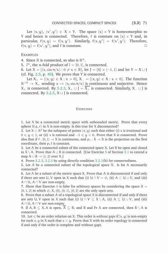
CONNECTED SPACES, COMPACT SPACES [3.3] 71
Let (x,y), (x ′,y′) ∈ X × Y. The space {x} × Y is homeomorphic toY and hence is connected. Therefore, f is constant on {x} × Y and, inparticular, f(x,y) = f(x,y′). Similarly, f(x,y′) = f(x ′,y′). Therefore,f(x,y) = f(x ′,y′), and f is constant. ✷
EXAMPLES
4. Since R is connected, so also is Rn.5. In, the n-fold product of I = [0, 1], is connected.6. Let X = {(x, sinπ/x) : 0 6= x ∈ R}, let J = {0} × [−1, 1] and let Y = X ∪ J(cf. Fig. 2.5, p. 40). We prove that Y is connected.
Let X+ = {(x,y) ∈ X : x > 0}, X− = {(x,y) ∈ X : x < 0}. The functionR>0 → X+ sending x 7→ (x, sinπ/x) is continuous and surjective. HenceX+ is connected. By 3.2.3, X+ ∪ J = X+ is connected. Similarly, X− ∪ J isconnected. By 3.2.5, X ∪ J is connected.
EXERCISES
1. Let X be a connected metric space with unbounded metric. Prove that every
sphere S(a, r) in X is non-empty. Is this true for X disconnected?
2. Let X ⊂ R2 be the subspace of points (x, y) such that either (i) x is irrational and
0 6 y 6 1, or (ii) x is rational and −1 6 y < 0. Prove that X is connected. Prove
also that if f : [0, 1]→ X is continuous, and p1 : X→ R is the projection on the first
coordinate, then p1f is constant.
3. Let A be a connected subset of the connected space X. Let B be open and closed
in X \ A. Prove that A ∪ B is connected. [Use Exercise 5 of Section 3.1 to extend a
map A ∪ B→ {1, 2} over X.]
4. Prove 3.2.3, 3.2.5 by using directly condition 3.2.1(b) for connectedness.
5. Let A be a connected subset of the topological space X. Is Int A necessarily
connected?
6. Let A be a subset of the metric space X. Prove that A is disconnected if and only
if there are sets U,V open in X such that (i) U ∩ V = ∅, (ii) A ⊂ U ∪ V, and (iii)
A ∩U, A ∩ V are non-empty.
7. Show that Exercise 6 is false for arbitrary spaces by considering the space X =
{0, 1, 2} in which ∅, X, {0}, {0, 1}, {0, 2} are the only open sets.
8. Prove that a subset A of a topological space X is disconnected if and only if there
are sets U,V open in X such that (i) U ∩ V ⊆ X \ A, (ii) A ⊆ U ∪ V, and (iii)
A ∩U,A ∩ V are non-empty.
9. If A,B ⊆ X,A is open, A ⊆ B, and B and Fr A are connected, then B \ A is
connected.
10. Let 6 be an order relation on X. This order is without gaps if ]x,y[ is non-empty
for each x,y in X such that x < y. Prove that X with its order topology is connected
if and only if the order is complete and without gaps.

72 [3.3] TOPOLOGY AND GROUPOIDS
3.3 Components and locally connected spaces
Let X be a topological space and let x ∈ X. The component of x in X is C(x),the union of all connected sets containing x. By 3.2.5, C(x) is connected;therefore, C(x) is the largest connected set containing x. But C(x) is alsoconnected [3.2.3]. Therefore, C(x) = C(x). This proves:
3.3.1 The component of x in X is a closed subset of X.
A component need not be open. For example, in the space L the componentof 0 is {0}, which is closed but not open in L. Again, the components ofpoints of Q are not open in Q. An obvious question is therefore: underwhat conditions are the components always open?
Definition A space X is locally connected at a point x in X if the connectedneighbourhoods of x form a base for the neighbourhoods at x. (This issometimes expressed as: x has a base of connected neighbourhoods.) Thespace X is locally connected if it is locally connected at each x in X. Thus Xis locally connected if, for each x in X, each neighbourhood of x contains aconnected neighbourhood of x.
One more definition: if A ⊆ X, the components of A are the componentsof the points of the subspace A. So the components of A are subsets of A,except that the empty set ∅ has no components.
3.3.2 X is locally connected if and only if the components of each open set of
X are open sets of X.
Proof Suppose X is locally connected, V is open in X, C is a component ofV , and x ∈ C. Since V is a neighbourhood of x, and X is locally connected,there is a connected neighbourhood U of x such that U ⊆ V . Therefore,U ⊆ C, and C is a neighbourhood of x. Therefore, C is open.
For the converse, we start with a neighbourhood V of x which we maysuppose to be open (otherwise we replace V by IntV). The component ofV which contains x is open in X (by assumption), and so is a connectedneighbourhood of x contained in V . ✷
A special case of 3.3.2 is that, if X is locally connected, then each com-ponent of X is open.
EXAMPLES
1. The following spaces are not locally connected: the rationals, Q; theirrationals, R \Q; and L = {0} ∪ {1/n : n ∈ N,n 6= 0}.
2. A connected set need not be locally connected: the space Y = X ∪ J ofExample 6, p. 71, is not locally connected, since points of J have no ‘small’connected neighbourhoods [cf. Fig. 3.2].

CONNECTED SPACES, COMPACT SPACES [3.3] 73
z
N
J ∩N
Fig. 3.2
In fact we leave as an exercise for the reader the detailed proof of thefollowing statement: if z ∈ J, there is in Y a neighbourhood N of z suchthat the component of z in N is N ∩ J.3. Let X consist of the line segment joining (1, 1) in R2 to the points ofL × {0} [Fig. 3.3]. Then X is connected, but not locally connected, since(0, 0) has no ‘small’ connected neighbourhoods. (Here also, we leave adetailed proof to the reader.) Is X \ {(1, 1)} connected?
(0, 0)
(1, 1)
Fig. 3.3
4. A discrete space is locally connected and also totally disconnected.
Cut points
Let f : X→ Y be a homeomorphism. If C is a component of a point x of X,then f[C] is a component of f(x) in Y: this follows from the fact that A ⊆ X

74 [3.3] TOPOLOGY AND GROUPOIDS
is connected if and only if f[A] is connected. Consequently, f induces abijection of the components of X to the components of Y. So the number ofcomponents of X is a topological invariant of X. However, this is not a verysubtle invariant, since it fails to distinguish different connected spaces.
Definition Let X be connected space, and k a natural number or N. Apoint x in X is a cut point of order k if X \ {x} has k components.
Let X be connected, and f : X→ Y a homeomorphism. A point x in X isa cut point of order k in X if and only if f(x) is a cut point of order k in Y.Therefore, the number of cut points of order k is a topological invariant ofX.
EXAMPLES
5. The closed interval [0, 1] has two cut points of order 1; the half-openinterval [0, 1[ has one cut point of order 1; the open interval ]0, 1[ has nocut points of order 1. Therefore, no two of the spaces [0, 1], [0, 1[ and ]0, 1[
are homeomorphic.6. The following 1-dimensional‡ spaces can be distinguished by the num-bers of cut points of various orders:
Fig. 3.4
7. These methods however fail to distinguish between the following spaces:
Fig. 3.5
However, if we remove two points from the first space, two componentsare left, while with the second space we can get one, two, or three compo-nents by removing different pairs of points. Hence, the two spaces are nothomeomorphic.8. The space Rn has cut points of order 1 only if n > 1. That is, if a ∈ Rn,then Rn\{a} is connected if n > 1. For let x,y ∈ Rn\{a}, and let z ∈ Rn\{a}
be such that the lines L,M joining z to x,y respectively do not pass througha (this is possible since n > 1). Then L ∪M is a connected set containing xand y, so that x and y belongs to the same component of Rn \ {a}.
‡The term 1-dimensional is to be understood at this stage only intuitively.

CONNECTED SPACES, COMPACT SPACES [3.3] 75
x
L
z
a
y
M
Fig. 3.6
This proves that Rn is not homeomorphic to R1 if n 6= 1. It is muchmore difficult to prove the Invariance of Dimension: if Rm is homeomor-phic to Rn, then m = n. All the present proofs of this theorem, as of theInvariance of Domain, use techniques of homology theory or of subdivisionsof simplicial complexes.
Actually, a stronger result than the Invariance of Dimension is true: iff : Rm → Rn is a continuous bijection, then m = n and f is a homeomor-phism.9. Another problem is to distinguish between surfaces, for example the 2-sphere S2 and the torus T2 = S1×S1. This latter space is homeomorphic tothe anchor ring [Fig. 3.7(ii)].
(i) S2 (ii) T2
B
A
Fig. 3.7
Since removing points is a useful method for distinguishing1-dimensional spaces, it seems reasonable that to distinguish 2-dimensionalspaces we need to remove 1-dimensional subspaces (supposing also that weknow what the words 1-dimensional and 2-dimensional mean). For exam-ple, let A be the meridian circle on T2; then T2\A has only one component.On the other hand, it seems likely that if B is any subspace of S2 homeo-morphic to S1, then S2 \ B has two components. This is equivalent to theJordan Curve Theorem: if B is a subspace of R2 homeomorphic to S1 (i.e., Bis a simple closed curve in R2) then R2 \ B has two components. We provethis in chapter 9.
As we shall see in chapter 9, S2 and T2 can be distinguished by their

76 [3.3] TOPOLOGY AND GROUPOIDS
fundamental groups.10. If two spaces are homeomorphic, they must have the same ‘local’ prop-erties. Let X be the graph of x 7→ sin(π/x), and let Y = X∪{(0, 0)}. Then Y isconnected, and any point of Y is a cut point of order 2. But Y is not home-omorphic to R, since R is locally connected, and Y is not locally connectedat (0, 0).11. We can also define local cut points. A point x in X is a local cut point oforder k if each neighbourhood V of x contains a connected neighbourhoodU of x such that U \ {x} has k components. If X is homeomorphic to Y, thenX and Y must have the same number of local cut points of order k for eachk = 1, 2, . . . . The spaces of Fig. 3.8 are distinguished by the fact that onehas a local cut point of order 4, and the other does not.
Fig. 3.8
By the use of homology theory these methods can be generalised tohigher dimensional spaces.
EXERCISES
1. Prove that if X has a finite number of components, then each component is open.
2. Prove that the space X of Exercise 2 of Section 3.2 is not locally connected.
3. Decide whether or not the following 1-dimensional spaces are homeomorphic
Fig. 3.9
4. Construct a locally connected subspace X of R2 in which for each r > 0 there is
an x in X such that B(x, r) (the open ball in X) is not connected.
5. Prove that Rn is locally connected.
6. Let X = (L× I) \ ({0}×]0, 1[). Prove that the components of (0, 0) and (0, 1) in X
are single points. Let f : X→ {1, 2} be continuous. Prove that f(0, 0) = f(0, 1).
7. Let X be the subspace of R2
{0} ∪ {(x, x sinπ/x) : x 6= 0}
with the Euclidean metric. Prove that if r > 0 is sufficiently small then B(0, r) (the
open ball in X) is not connected.
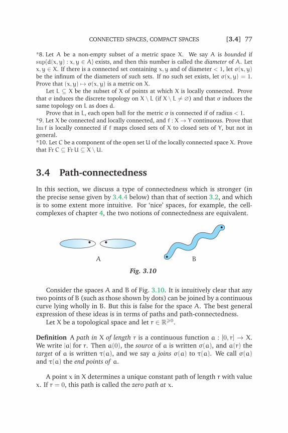
CONNECTED SPACES, COMPACT SPACES [3.4] 77
*8. Let A be a non-empty subset of a metric space X. We say A is bounded if
sup{d(x,y) : x,y ∈ A} exists, and then this number is called the diameter of A. Let
x,y ∈ X. If there is a connected set containing x,y and of diameter < 1, let σ(x, y)
be the infinum of the diameters of such sets. If no such set exists, let σ(x,y) = 1.
Prove that (x,y) 7→ σ(x, y) is a metric on X.
Let L ⊆ X be the subset of X of points at which X is locally connected. Prove
that σ induces the discrete topology on X \ L (if X \ L 6= ∅) and that σ induces the
same topology on L as does d.
Prove that in L, each open ball for the metric σ is connected if of radius < 1.
*9. Let X be connected and locally connected, and f : X→ Y continuous. Prove that
Im f is locally connected if f maps closed sets of X to closed sets of Y, but not in
general.
*10. Let C be a component of the open setU of the locally connected space X. Prove
that FrC ⊆ FrU ⊆ X \U.
3.4 Path-connectedness
In this section, we discuss a type of connectedness which is stronger (inthe precise sense given by 3.4.4 below) than that of section 3.2, and whichis to some extent more intuitive. For ‘nice’ spaces, for example, the cell-complexes of chapter 4, the two notions of connectedness are equivalent.
A B
Fig. 3.10
Consider the spaces A and B of Fig. 3.10. It is intuitively clear that anytwo points of B (such as those shown by dots) can be joined by a continuouscurve lying wholly in B. But this is false for the space A. The best generalexpression of these ideas is in terms of paths and path-connectedness.
Let X be a topological space and let r ∈ R>0.
Definition A path in X of length r is a continuous function a : [0, r] → X.We write |a| for r. Then a(0), the source of a is written σ(a), and a(r) thetarget of a is written τ(a), and we say a joins σ(a) to τ(a). We call σ(a)and τ(a) the end points of a.
A point x in X determines a unique constant path of length r with valuex. If r = 0, this path is called the zero path at x.

78 [3.4] TOPOLOGY AND GROUPOIDS
It is important to note that a path in X is not just a set of points, but is afunction. For example, the two paths [0, 1]→ R given by t 7→ t and t 7→ t2
are distinct paths in R joining 0 to 1. Our illustrative figures should thenshow the graph of a path—but it is usually more convenient to illustratethe image of the path.
We now consider two simple operations on paths. The reverse of a patha : [0, r]→ X is the path
−a : [0, r]→ X
t 7→ a(r− t).
Thus |− a| = |a| and −a joins τ(a) to σ(a).
σ(a)
a
τ(a)
τ(−a)
−a
σ(−a)
Fig. 3.11
The reverse of a path is always defined. On the other hand, the sum
b + a of two paths is defined if and only if the final point of a coincideswith the initial point of b (that is, if and only if τ(a) = σ(b)). In such case,b+ a is the path
b+ a : [0, |b|+ |a|]→ X
t 7→{a(t), 0 6 t 6 |a|
b(t− |a|), |a| 6 t 6 |a|+ |b|.
Clearly the condition τ(a) = σ(b) is essential for b + a to be defined; andwith this condition, b+ a is continuous by the gluing rule [2.5.12].
σ(b + a) = σ(a)
a
τ(a) = σ(b)
b
τ(b + a) = τ(b)
Fig. 3.12
We use the additive notation because of its convenience in dealing withdifferences (b− c is a good abbreviation of b+ (−c)). Our convention thatb + a means first a then b [Fig. 3.12] is related to the convention that thecomposition gf of functions means first apply f, then apply g.

CONNECTED SPACES, COMPACT SPACES [3.4] 79
The reader should be warned that addition of paths is not commutative:if b + a is defined, then a+ b need not be defined. And even if both b + a
and a+ b are defined, they are in general unequal.
Definition A topological space X is path-connected if for any x,y in X, thereis a path in X joining x to y.
EXAMPLE
1. We recall that a subset A of a normed vector space V is convex if, for anyx,y in A, the line segment
[x,y] = {(1− t)x+ ty : 0 6 t 6 1}
is contained in A. A convex set A is path-connected, since if x,y ∈ A thent 7→ (1− t)x+ ty is a path in A from x to y of length 1. Examples of convexsets are B(x, r), E(x, r). For example, if y, z ∈ B(x, r) and 0 6 t 6 1, then
‖(1− t)y+ tz− x‖ 6 ‖(1− t)(y− x)‖+ ‖t(z− x)‖< (1− t)r+ tr = r
whence (1− t)y+ tz ∈ B(x, r). Again, any interval of R is convex.
Other examples of path-connected sets may be constructed from thefollowing results.
3.4.1 Let f : X→ Y be continuous and surjective. If X is path-connected, thenso also is Y.
Proof Let y,y′ ∈ Y; then there are points x, x ′ in X such that f(x) = y,f(x ′) = y′. Since X is path-connected, there is a path a joining x to x ′.Then fa joins y to y′. ✷
3.4.1 (Corollary 1) Let X be homeomorphic to Y. Then X is path-connected ifand only if Y is path-connected.
3.4.2 Let (Aλ)λ∈Λ be a family of path-connected subspaces of X such that⋂λ∈ΛAλ is non-empty. Then A =
⋃λ∈ΛAλ is path-connected.
Proof Let x,y ∈ A, z ∈⋂
λ∈ΛAλ, and suppose x ∈ Aλ, y ∈ Aµ. SinceAλ is path-connected, there is a path a joining x to z. Since Aµ is path-connected, there is a path b joining z to y. Then b + a is a path joining xto y. ✷
3.4.3 If X, Y are path-connected, then X× Y is path-connected.

80 [3.4] TOPOLOGY AND GROUPOIDS
Proof Let (x,y), (x ′,y′) ∈ X× Y. Let a be a path in X joining x to x ′, b bea path of Y joining y to y′. Then t 7→ (a(t),y) joins (x,y) to (x ′,y), andt 7→ (x ′,b(t)) joins (x ′,y) to (x ′,y′). The sum of these paths joins (x,y) to(x ′,y′). ✷
We can use 3.4.2 to define path-components of X: if x ∈ X, then thepath-component of x is the union of all path-connected subsets P of X suchthat P contains x. This union will be a path-connected by 3.4.2, and willcontain x. Hence it is the largest path-connected subset of X containing x.
A path-component need not be closed. To show this, we consider a littlethe relationship between the two kinds of connectedness.
3.4.4 If X is path-connected, then X is connected.
Proof Let x,y ∈ X, and let a be a path joining x to y. Then Ima is by 3.2.2a connected set containing x and y. Hence x and y belong to the samecomponent of X. Thus X has only one component, and must be connected.
✷
EXAMPLE
2. Let Y = X ∪ J be the connected space of Example 2, p. 72 and Example6, p. 71. Then Y is not path-connected.
Proof Let g : Y → {0, 1} be the function which sends points of J to 0 andpoints of X to 1. Of course, g is not continuous, but we prove that for anypath f : [0, r]→ Y, the composite gf is continuous.
Let x ∈ [0, r]. If fx ∈ X, then fx has a neighbourhood N which doesnot meet J; hence there is a neighbourhood M of x such that f[M] ⊂ N,whence gf[M] = {1}; continuity of gf at x follows easily.
On the other hand, suppose fx ∈ J. As stated on p. 72, there is aneighbourhood (in Y) of fx such that the component of fx in N is N ∩ J.Therefore, there is a connected neighbourhood M of x such that f[M] ⊆N ∩ J. Hence, gf[M] = {0}, and continuity of gf at x follows easily.
We have now proved that gf is continuous. Since [0, r] is connected itfollows that gf is constant. So Im f is contained either in X or in J, and Y isnot path-connected. ✷
The philosophy of local path-connectedness is different from that oflocal connectedness. The definition of the former concept that first suggestsitself is that a space X is locally path-connected if each point x in X has abase of path-connected neighbourhoods. However, because of extensionsof this property to higher-dimensional kinds of connectedness, we take adifferent definition which, it turns out, is equivalent to the above.

CONNECTED SPACES, COMPACT SPACES [3.5] 81
Definition A space X is locally path-connected if, for each point x in X, anyneighbourhood of U of x contains a neighbourhood V of x such that anytwo points of V can be joined by a path in U.
3.4.5 A space X is locally path-connected ⇔ each point of X has a base of
open path-connected neighbourhoods.
Proof The implication ⇐ is trivial, and so we prove the implication ⇒.Let x ∈ X and let U be an open neighbourhood of x. Let U′ be the path-component of U containing x.
Let y ∈ U′. Then U is a neighbourhood of y, and so U contains aneighbourhood V of y such that any two points of V can be joined by a pathinU. This implies that V is contained inU′. HenceU′ is a neighbourhood ofy. Therefore (since x ∈ U′) U′ is an open, path-connected neighbourhoodof x. ✷
EXERCISES
1. In the following, X is a subspace of R2 and x0, x1 are points of X. Write down, if
possible, explicit paths in X joining x0 to x1.
(i) X = {(x,y) ∈ R2 : |x| > 1 or |y| > 1}, x0 = (−2, 0), x1 = (2, 0).
(ii) X = {(x,y) ∈ R2 : x+ y 6= 1}, x0 = (4,−5), x1 = (−6, 8).
(iii) X = {(x,y) ∈ R2 : [x] = [y]}, x0 = (− 12,−1), x1 = (1, 3
2).
(iv) X = {(x,y) ∈ R2 : [x] + [y] = 1}, x0 = ( 32, 0), x1 = (0, 3
2).
2. Let V be a normed vector space over R. A ‘bent line’ in V is the union of a finite
number of line segments [ui,ui+1], i = 1, . . . ,n − 1, and such a bent line is said to
join u1 to un. A subset A of V of ‘polygonally connected’ if, for any two points u, v
of A, there is a bent line joining u to v and lying wholly in A.
Prove that any open, connected subset of V is polygonally connected. Give
examples of subsets of R2 which are path-connected but not polygonally connected.
3. Let X = {a,b, c} with the topology whose open sets are ∅, {c}, {a, c}, {b, c},X.
Prove that X is path-connected.
4. Prove that X is locally path-connected if and only if the path-components of each
open set of X are open. Give an example of a space which is path-connected but not
locally path-connected.
5. Prove that two points x,y in X lie in the same path-component if and only if they
can be joined by a path of length 1.
6. Let V be a normed vector space over R of dimension > 1. Prove that S(V) is
path-connected.
7. Prove that if X is a countable subset of Rn (n > 1), then Rn\X is path-connected.
8. Let X1,X2 be subsets of X such that X = IntX1 ∪ IntX2. Prove that, if X is
path-connected, then each path-component of X1 meets X2.

82 [3.5] TOPOLOGY AND GROUPOIDS
3.5 Compactness
The reader will certainly be aware of the importance for mathematics ofthe distinction between finite and infinite sets. As examples, consider thestatements (a) the sum of elements of a set of A of real numbers is well-defined, (b) a setA of real numbers has a least element, (c) the intersectionof the elements of a set A of open sets is open. Each of these is true ifA is finite but may be false if A is infinite. This wide range of techniquesapplicable to finite sets but not infinite ones is the reason for the importanceof the notion of a compact space in topology.
In order to define compactness we need some preliminary definitions.
Let X be a topological space. A cover of X is a set A of sets such that theunion of the elements of A contains X. A subcover of A is a subset B of Asuch that B covers X. A cover A of X is open if each set of A is open in X.
EXAMPLES
1. Let k ∈ R>0, and let A be the set of intervals ]x−k, x+k[ for each x ∈ R.Then A is an open cover of R. Similarly, in any metric space X, the set ofall open balls B(x, k), x ∈ X, is an open cover of X.2. Let X be a metric space and let x ∈ X. The set of open balls B(x,n) forall positive n in N is an open cover of X.3. The set of intervals ]1/n, 1] for n a positive integer, is an open cover of]0, 1].4. If A is an open cover of Y, and f : X → Y is continuous, then the set off−1[A] for all A in A is an open cover of X.5. For any topological space X, the set {X} is an open cover of X as is {X,∅}.
Definition A topological space X is compact if every open cover of X has afinite subcover.
This means of course, that to prove a space X is compact we have tostart with any open cover A of X and construct a finite subcover of A. Toprove X non-compact, we have to produce an open cover A of X withoutfinite subcover.
EXAMPLES
6. An infinite discrete space X is not compact, since the set of singletons{x} for each x in X is an open cover of X without finite subcover.7. Any finite space X is compact, since any open cover of X is a finite set.8. The interval ]0, 1] is not compact—the open cover of Example 3 has nofinite subcover.9. If X is a metric space with unbounded metric, then X is not compact. Toprove this, let x ∈ X and consider the open cover of Example 2. This cover

CONNECTED SPACES, COMPACT SPACES [3.5] 83
has a finite subcover if and only if X = B(x,n) for some n, in which case Xhas bounded metric.10. The previous example has a converse, namely, that if X is a non-compact metric space, then X admits an equivalent unbounded metric. Theproof of this theorem is not as simple as that of its converse.
Compactness is a topological invariant. In fact, we have the strongerresult.
3.5.1 Let X be compact and f : X → Y continuous and surjective. Then Y is
compact.
Proof Let A be an open cover of Y. Since f is continuous the set B of setsf−1[A] for all A in A is an open cover of X. Since X is compact, B hasa finite subcover C. The set of A in A for which f−1[A] is in C is a finitesubcover of A. ✷
3.5.2 Remark
Let C be a subspace of the topological space X. Then we have covers of Cby sets open in X, and by sets open in C. We distinguish these by callingthem open covers of the set C, and of the space C, respectively. An opencover of the space C clearly consists of sets A ∩ C for A in an open coverof the set C. So the statements (a) every open cover of the space C has afinite subcover, and (b) every open cover of the set C has finite subcover,are equivalent, and either may be used as a criterion for compactness of C.
3.5.3 Remark
Let A be a cover of the space X. A refinement of A is a cover B of X suchthat each set of B is contained in some set of A. Suppose B is an opencover which refines an open cover A. Then, if B has a finite subcover, soalso does A. Thus, when trying to construct finite subcovers of an opencover A we may at will replace A by an open refinement.
The next theorem gives the simplest non-trivial example of a compactspace. (The proof given here is due to R. M. F. Moss and G. Roberts.)
3.5.4 The unit interval I is compact.
Proof Let A be an open cover of I. For each x in I we choose an intervalUx, open in I, such that Ux contains x and is contained in some set of A.The set B of these intervals Ux is an open cover of I which refines A. ByRemark 3.5.3, we may assume from that start that each element of A is aninterval.

84 [3.5] TOPOLOGY AND GROUPOIDS
Let f : I→ {0, 1} be the function defined by fx = 0 if [0, x] can be coveredby a finite number of sets of A, and fx = 1 otherwise. We shall prove thatf is constant on each set of A.
Let U ∈ A, let x ∈ U and suppose fx = 0. Then [0, x] is covered by afinite subset B of A and so for any y in U, since U is an interval [0,y] iscovered by the finite set B ∪ {U}. Thus we have shown, as required, that fis 0 either on all or none of U.
It follows immediately that f is continuous; therefore, f is constant(since I is connected) and the image of f is {0} (since f0 = 0). Hence[0, 1] can be covered by a finite number of sets of A. ✷
It is instructive to examine the failure of similar attempts to prove thatthe intervals ]0, 1] and [0, 1[ are compact (they are non-compact by Example8 and a similar example for [0, 1[). The proof for ]0, 1] breaks down becausewe cannot prove that the unique value of f is 0. The proof for [0, 1[ breaksdown because f1 is not defined.
3.5.5 A closed subset of a compact space is compact.
Proof Let C be a closed subset of the compact space X and, applying 3.5.2,let A be an open cover of the set C. Since X \ C is open,
A′ = A ∪ {X \ C}
is an open cover of X. By compactness of X, A′ has a finite subcover B say.
Here B is an open cover of X, and so an open cover of the set C. IfB does not contain X \ C, then B is a finite subcover of A. In any case,B \ {X \ C} is certainly a finite subcover of A. ✷
The next theorem has a slightly complicated formulation—this is due tothe fact that we wish to include in one theorem (and one proof) a numberof highly important special cases.
3.5.6 Let B,C be compact subsets of X, Y respectively, and let W be a cover
of B × C by sets open in X × Y. Then B,C have open neighbourhoods U,Vrespectively such that U× V is covered by a finite number of sets of W.
Proof The proof is carried out in two steps, first when B has a single pointb, and next for B arbitrary.
Step 1− B = {b}

CONNECTED SPACES, COMPACT SPACES [3.5] 85
cNc Wc
{b}× C
Mc
b X
Fig. 3.13
For each c in C there are open neighbourhoods of Mc of b (in X), Nc
of c (in Y) such that Mc × Nc is contained in some set Wc of W. The set{Nc : c ∈ C} is an open cover of the set C which, by compactness, has afinite subcover {Nf : f ∈ F}. Let
U =⋂
f∈F
Mf, V =⋃
f∈F
Nf.
Since F is finite, U is an open neighbourhood of b. Clearly,
{b}× C ⊆ U× V ⊆⋃
f∈F
Wf.
Step 2− B arbitrary
By step 1, for each b in B there are open neighbourhoods Ub of b (inX), Vb of C (in Y), such that Ub × Vb is contained in a finite union, say⋃{Wf : f ∈ Fb}, of sets of W. The set {Ub : b ∈ B} is an open cover of B
which, by compactness, has a finite subcover {Ug : g ∈ G}. Let
U =⋃
g∈G
Ug, V =⋂
g∈G
Vg.
Then U,V are open neighbourhoods of B,C respectively and U× V is con-tained in the union of the finite number of sets Wf, f ∈ Fg,g ∈ G. ✷
3.5.6 (Corollary 1) The product of compact spaces is compact.
Proof This follows from 3.5.6 by taking B = X, C = Y (and so U = X,V = Y). ✷
3.5.6 (Corollary 2) Let B,C be compact subsets of X, Y respectively, and letW

86 [3.5] TOPOLOGY AND GROUPOIDS
be an open subset of X×Y containing B×C. Then B,C have open neighbour-hoods U,V respectively such that U× V ⊆W.
Proof This is the case of 3.5.6 when W = {W}. ✷
3.5.6 (Corollary 3) If B,C are disjoint compact subsets of the Hausdorff space
X, then B,C have disjoint open neighbourhoods.
Proof In 3.5.6 (Corollary 2), let X = Y and W = (X× X) \∆[X] where ∆ isthe diagonal of X × X;W is open since X is Hausdorff. Since B and C aredisjoint, B × C is contained in W. By 3.5.6 (Corollary 2), B,C have openneighbourhoods U,V such that U× V ⊆W. Hence U ∩ V = ∅. ✷
3.5.6 (Corollary 4) A compact subset of a Hausdorff space is closed.
Proof Let C be a compact subset of the Hausdorff space X, and let x ∈ X\C.By 3.5.6 (Corollary 3), x and C have disjoint neighbourhoods. Hence X \Cis open. ✷
As an application of these rules we prove
3.5.7 A subset of Euclidean n-space Rn is compact if and only if it is closedand bounded.
LetA be a closed, bounded subset of Rn. Let Jr be the subspace of Rn ofpoints (x1, . . . , xn) such that |xi| 6 r—thus Jr is the product of the interval[−r, r] with itself n times [cf. Exercise 8 of Section 2.4]. The interval [−r, r]is homeomorphic to [0, 1] (if r > 0) and so is compact. By 3.5.6 (Corollary1), Jr is compact. Since A is bounded, it is contained in Jr for some r. ThusA is a closed subset of a compact space and so is compact.
The converse follows from Example 9 and 3.5.6 (Corollary 4). ✷
EXAMPLES
11. The Cantor set K [The Example of Section 1.3] is a closed, boundedsubset of R and so is compact.12. The subsets of Rn (with the Euclidean norm)
Sn−1 = {x ∈ Rn : ‖x‖ = 1},
En = {x ∈ Rn : ‖x‖ 6 1}
are both closed, bounded subsets of Rn and so are compact.13. If X is indiscrete, then any subset A of X is compact, but A will beclosed in X only if A = ∅ or A = X.

CONNECTED SPACES, COMPACT SPACES [3.5] 87
14. Let W be the subspace of R2 of points (x,y) such that y > |x|. LetB = {0}, C = ]0, 1]. Then W is an open set of R2 containing B×C but, if Uis a neighbourhood of 0, then W does not contain even U× C.
A map f : X → Y of spaces is called closed if f[C] is closed in Y for eachclosed set C of X. For example, a continuous bijection f : X→ Y is closed ifand only if f is a homeomorphism.
3.5.8 Any map from a compact space to a Hausdorff space is closed.
Proof Let f : X → Y be a map where X is compact and Y is Hausdorff. LetC be closed in X. Then C is compact [3.5.5] whence f[C] is compact [3.5.1]and so f[C] is closed [3.5.6 (Corollary 4)]. ✷
3.5.8 (Corollary 1) A continuous bijection from a compact space to a Haus-
dorff space is a homeomorphism.
Proof If f is a closed bijection, then f−1 is continuous. ✷
The following proposition is required later; the simple proof is left as anexercise.
3.5.9 A topological space which is a finite union of compact spaces is itself
compact.
There is a characterisation of compactness by means of closed sets whichis of great importance in some contexts but not, as it turns out, in this book.For this reason it has been left as an exercise [Exercise 10].
There is a generalisation of 3.5.6 which uses the product topology de-fined in section 5.7:
3.5.10 (Tychonoff ’s theorem) The topological product of any family of com-
pact spaces is compact.
This theorem is of great importance in functional analysis and in a fur-ther study of some of the topics in this book. However the theorem is notessential to our present purposes, and so we refer the reader to [Kel55] or[Dug68] for a proof.
EXERCISES
1. Give an example of a space with two points in which not all compact sets are
closed.
2. Prove that R with the Zariski topology is compact.
3. Prove that a discrete space is compact if and only if it is finite.

88 [3.6] TOPOLOGY AND GROUPOIDS
4. Use the result of sections 3.2 and 3.5 to prove that if a,b ∈ R (a < b) and
f : [a,b]→ R is continuous, then Im f is a closed, bounded interval.
5. Let X be a compact topological space, and f : X → R a continuous function.
Prove that there are elements a,b in X such that f(a) = inf(Im F), f(b) = sup(Im f).
Deduce that if f(x) > 0 for all x in X, then there is a positive real number r such
that f(x) > r for all x in X.
6. Let X = R × Y where Y is an indiscrete space with two elements a,b. Prove
that in X the sets A = [0, 1[×{a} ∪ [1, 2]× {b}, B = [0, 1] × {a}∪ ]1, 2] × {b} are both
compact, but A ∩ B is non-compact.
7. Let (Ci)i∈I be a family of closed, compact subsets of X. Prove that ∩i∈ICi is
compact.
8. Let A,B be non-empty subsets of the metric space X. Let
dist(A,B) = inf{(d(a,b) : a ∈ A,b ∈ B}.
Prove that ifA,B are disjoint and closed, andA is compact, then there is an element
a of A such that
dist(A,B) = dist(a,B) > 0.
9. Prove that I2 with the television topology is compact, connected and Hausdorff.
10. Prove that the following conditions on a topological space X are equivalent. (i)
X is compact. (ii) If (Ci)i∈I is a family of closed subsets of X such that ∩i∈ICi = ∅,
then ∩a∈ACa = ∅ for some finite subset A of I. (iii) If (Ci)i∈I is a family of closed
subsets of X such that ∩a∈ACa 6= ∅ for all finite subsets A of I, then ∩i∈ICi 6= ∅.
11. Let F : Rn → V be a linear isomorphism, where Rn is Euclidean space and
V is a normed vector space over R. Prove that the function h : Sn−1 → R which
sends x 7→ ‖f(x)‖ is continuous, and that there is a positive real number δ such that
h(x) > δ for all x in Sn−1. Show that for all y in V, |f−1(y)| 6 δ−1‖y‖. Finally, prove
that f is a homeomorphism.
12. Prove that n-dimensional complex space Cn is linearly homeomorphic to R2n.
Prove that, if V is a finite dimensional normed vector space over R or C, then all
norms on V are equivalent. [This theorem is proved in [Die60] by completeness
methods. An advantage of such methods is that they also prove that any finite
dimensional subspace of a normed vector space V is closed in V.]
13. Let Xn be the subset {n−1}× [−n,n] of R2 and let Y = R2 \∪n>1Xn. Prove that
Y is connected but not path-connected.
*14. Let ϕ : X × C → R be a map where C is compact. Prove that the function
x 7→ supc∈C ϕ(x, c) is a continuous function X→ R.
3.6 Further properties of compactness
The basic results on compactness are given in the last section. The moretechnical results of this section will be used in later chapters, but the studyof these results can be omitted till they are needed.

CONNECTED SPACES, COMPACT SPACES [3.6] 89
Locally compact spaces, normal spaces
Definition A topological space X is locally compact if each x in X has a baseof compact neighbourhoods.
EXAMPLES
1. Euclidean n-space Rn is locally compact since, if x ∈ Rn, then the closedballs E(x, r) for r > 0 are compact and form a base for the neighbourhoodsof x.2. The space Q of rational numbers is not locally compact since a neigh-bourhood of 0 in Q cannot be closed in R and so cannot be compact.
In the literature, it is common to define a space X to be locally compactif each point of X has a compact neighbourhood. We have not adopted thisdefinition for two reasons:(i) It would be contrary to the general spirit of local properties. If P is aproperty of topological spaces, it is usual to say X is locally P if each pointof X has a base of neighbourhoods with property P.(ii) The property of locally compact spaces needed later is exactly the onewe have taken for a definition.
For Hausdorff spaces the two definitions are equivalent. This is an easyconsequence of the following result.
3.6.1 A compact Hausdorff space is locally compact.
Proof Let X be compact and Hausdorff, let x ∈ X and let W be an openneighbourhood of x. We must find a compact neighbourhood of x containedin W.
Let C = X\W. Then C is closed in X and so is compact. By 3.5.6 (Corol-lary 3), x and C have disjoint open neighbourhoods M,N say. The closureM of M is contained in X \ N which is itself contained in W. Also M iscompact (since it is closed in X) and is a neighbourhood of x. ✷
Definition A topological space X is normal if disjoint closed sets of X havedisjoint neighbourhoods.
It is immediate from 3.5.5 and 3.5.6 (Corollary 3) that any compact,Hausdorff space is normal. We showed in section 2.9 that any metric spaceis normal.
Normal spaces have another property important in many parts of topol-ogy, for example in metrisation theorems and in the theory of ANRs. Thefollowing theorem will be found in many texts.
3.6.2 (Tietze extension theorem) A space X is normal if and only if for any
closed subspaceC of X any map f : C→ I extends over X (i.e., is the restriction
of a map X→ I).

90 [3.6] TOPOLOGY AND GROUPOIDS
The proof that the extension condition implies normality is easy sincelet C = C1 ∪ C2 where C1,C2 are disjoint, non-empty closed subsets of Xand let f : C → I be 0 on C1 and 1 on C2. Let g : X→ I be an extension off over X. Then, for each r in ]0, 1[, the sets
g−1[0, r[, g−1]r, 1]
are disjoint open sets containing C1,C2 respectively; in fact for various rthese sets form a kind of ‘continuous family’ of open sets between C1 andC2. One word of warning—it is not always possible to find g such thatC1 = g−1[0], C2 = g−1[1]; conditions for this will be mentioned in theExercises.
Proper maps
Definition Let f : X → Y be a map of topological spaces. Then f is proper
if, for all spaces Z,f× 1 : X× Z→ Y × Z
is a closed map.
By taking Z to consist of a single point, we see that a proper map isalways closed. Similarly, to say that a constant map X → {y} is proper isequivalent to saying that for all Z the projection X × Z → Z is closed. Theresult on proper maps that we shall need (in section 5.8) is the followingand its corollary.
3.6.3 If f : X → Y is a closed map such that f−1[y] is compact for each y in
Y, then f is proper.
Proof Let h = f×1 : X×Z→ Y×Z, let C be a closed subset of X×Z, and letD = h[C]—we must prove thatD is closed, i.e., that the setD′ = (Y×Z)\Dis open.
Let (y, z) ∈ D′. Since the complement of f[X] × Z is open, we mayassume y ∈ f[X]. Let C′ = (X×Z)\C, so that C′ is open. It is easily verifiedthat
f−1[y]× {z} ⊆ C′
and so, by our assumptions and 3.5.6 (Corollary 2), there are open setsU,V such that
f−1[y]× {z} ⊆ U× V ⊆ C′.
Let U′ = X \ U, V ′ = Z \ V . Then C ⊆ (U′ × Z) ∪ (X× V ′) and so
D = h[C] ⊆ (f[U′]× Z) ∪ (f[X]× V ′) = Q say.

CONNECTED SPACES, COMPACT SPACES [3.6] 91
Since f is a closed map, Q is a closed set. Therefore,Q′ = (Y ×Z) \Q is anopen set contained in D′. But y /∈ f[U′], nor does z ∈ V ′, so it follows that(y, z) ∈ Q′. Hence D′ is open. ✷
The converse of 3.6.3 is true [see the Exercises], but will not be neededhere.
3.6.3 (Corollary 1) Any map from a compact space to a Hausdorff space is
proper.
Proof Let f : X→ Y be a map where X is compact and Y is Hausdorff. Thenf is closed by 3.5.8. If y ∈ Y, then {y} is closed in Y; hence f−1[y] is closedin X and so f−1[y] is compact. ✷
Lebesgue covering lemma
Let X be a metric space and A an open cover of X. We consider the followingquestion: is there a real number r > 0 such that the open cover Br =
{B(x, r) : x ∈ X} refines A? Clearly the set of all r for which this is so isan interval L of R, and L may be empty. If L is non-empty, then the realnumber l = sup L is called the Lebesgue number of the cover, A (we allowthe rather boring case l = ∞, which, intuitively, means A has lots of largesets).
EXAMPLES
3. If A = Br then the Lebesgue number of A is r.4. Let X = R, and let A consist of the open intervals ]n,n + 2[ for eachn ∈ Z. Then the Lebesgue number of A is 1
2.
5. Let X = ]0, 1[ and let A consist of the open intervals ]n−1, 1[ for allpositive integral n. Then A has no Lebesgue number.6. Let X = [0, 2]\ {1}, and let A consist of the intervals [0, 1[ and ]1, 2]. ThenA has no Lebesgue number.
3.6.4 (Lebesgue covering lemma) If X is a compact metric space, then any
open cover of X has a Lebesgue number.
Proof Let A be an open cover of X. Since X is compact, A has a finite sub-cover and any refinement of this is a refinement of A. So we may assumeA finite.
For each A in A and x in X let
fA(x) = dist(x,X \A),
f(x) = max{fA(x) : A ∈ A}.
Each fA is continuous and hence f is continuous.

92 [3.6] TOPOLOGY AND GROUPOIDS
If x ∈ X then x ∈ A for some A in A and for that A, fA(x) > 0 (sinceX \A is closed). Hence f(x) > 0 for all x in X.
The set f[X] is a compact and hence closed subset of R. Therefore,r = inf f[X] belongs to f[X], and so r > 0.
If x ∈ X then f(x) > r whence fA(x) > r for some A in A and so, bydefinition of fA, B(x, r) ⊆ A. This proves that the cover Br refines A. ✷
We now illustrate the main type of application of 3.6.4. Let a : [0, r] →Z be a path in a topological space Z. A subdivision of a is a sequencea1, . . . ,an (for some n) of paths in Z such that
a = an + · · ·+ a1. (*)
Such a subdivision is usually denoted by the expression (*).
3.6.4 (Corollary 1) Let U be an open cover of Z and a : [0, r]→ Z a path in Z.
Then there is a subdivision a = an + · · ·+ a1 such that for each i = 1, . . . ,n,
Imai is contained in some set of U.
Proof Let δ be the Lebesgue number of the covering {a−1[U] : U ∈ U} ofthe compact metric space [0, r]. Let n be an integer such that 0 < r/n < 1
2δ,
and let ai+1 be the path t 7→ a(t + ir/n), i = 0, . . . ,n − 1 of length r/n.Then clearly a = an + · · · + a1. Further, for each i = 0, . . . ,n − 1, theinterval [ir/n, (i+ 1)r/n] is contained in some set a−1[U], U ∈ U; hence
Imai = a[ir/n, (i+ 1)r/n] ⊆ U.
✷
Compactifications
If K is a compact space, then removing points from K is liable to produce anon-compact space. The idea of compactification is the reverse procedure—given a space X, can points be added to X to produce a compact space?There are a variety of such compactifications. They will not be used else-where in this book, but their importance is such that a brief survey shouldbe given of the ramifications.
The simplest compactification is the Alexandroff one-point compactifica-
tion X+ of X. Here X+ = X ∪ {ω}, where ω is a point not in X, with thetopology in which X is a subspace and the neighbourhoods of ω are thecomplements in X+ of closed compact subsets of X. A precise definitionis given in Exercise 6, and the principal properties are summarised in Ex-ercises 6–17. From these properties it can be shown that the one-pointcompactification of Rn is homeomorphic to the n-sphere Sn.

CONNECTED SPACES, COMPACT SPACES [3.6] 93
Another important compactification, but for which it is difficult to finda textbook exposition, is the Freudenthal compactification X∧. The intuitiveidea is that the open interval ]0, 1[ should be compactified by adding twoends, for example by adding 0 and 1 to give the closed interval [0, 1]. Theplane should be compactified by adding one end, as in the Alexandroff com-pactification. On the other hand, the following infinitely branched space iscompactified with an infinite number of ends.
Fig. 3.14
The definition of the ends of a space involves the number of componentsremaining when compact subsets are removed. The Freudenthal compacti-fication X∧ is defined for a Hausdorff space X which has a base of open sets(chapter 5) with compact boundary. Then X∧ \ X is a compact space con-taining X as a subspace and such that X∧\X is zero-dimensional. For a goodaccount in English, see [Hou74]. The number of ends of a covering spaceof a cell complex (see chapter 10) has important relations to group theory(see the articles [Hou74], [SW79] and the introductory article [Sch79]).The most striking recent result in the area is [Dun85].
A very large compactification of a space X is the Stone-Cech compact-ification βX. There is a map i : X → βX with the property that (i) βX iscompact and Hausdorff, (ii) if g : X → Y is any map to a compact Haus-dorff space Y, then there is a unique map g′ : βX→ Y such that g′i = g. Itis this universal property which gives this compactification its importance,particularly in analysis. The map i : X→ βX is an embedding if and only ifX is completely regular, that is, X is T0 and for each point x of X and closedsubset A of X not containing x, there is a continuous function f : X→ [0, 1]
such that f(x) = 0 and f[A] = {1}. For more information, see [Wal74]and [Joh82]. The reader should be warned that β applied to even a sim-ple space such as the positive integers N yields a horrendously complicatedspace which has been the subject of many papers.

94 [3.6] TOPOLOGY AND GROUPOIDS
For information on other compactifications, follow up the references in[IK87].
EXERCISES
1. Prove that the product of two locally compact spaces is locally compact.
2. Prove that a closed subspace of a locally compact space is locally compact, but
that an arbitrary subspace of a locally compact space need not be locally compact.
3. Let A be a compact subspace of a locally compact space, and let W be a neigh-
bourhood of A. Prove that there is a compact neighbourhood M of A such that
M ⊆W.
4. A space X is a k-space if a subset A of X is closed in X if and only if A ∩ C is
closed in C for every compact subset C of X. Prove that a locally compact space if
a k-space, as is any sequential space [Exercise 5 of Section 2.10]. Prove that the
space X of Exercise 4 of Section 2.9 is not a k-space.
5. Show that the following statement is true if f is open but not in general: if X is
locally compact and f : X→ Y is a continuous surjection, then Y is locally compact.
*6. The Alexandroff 1-point compactification. Let X be a topological space, letω be a
point not in X and let X∗ = X∪ {ω}. Define a neighbourhood topology on X∗ by (i) if
x ∈ X andM is a neighbourhood in X of x, thenM andM∪{ω} are neighbourhoods
in X∗ of x; (ii) if A is a closed compact subset of X, then X∗ \A is a neighbourhood
of ω. Prove (a) X∗ is compact and X is a subspace of X∗, (b) X is locally compact
and Hausdorff ⇔ X∗ is Hausdorff, (c) if X∗ is Hausdorff and i1 : X → X∗1 is any
homeomorphism into a compact Hausdorff space X∗1 such that the image of i1 is
the complement of a single point of X∗1, then there is a unique homeomorphism
g : X∗ → X∗1 such that gi = i1, where i : X→ X∗ is the inclusion. Prove also that, if
X is compact, then X∗ = X ⊔ {ω}. [The point ω is called the point at infinity of X∗.]
7. Given an open cover U of X, prove that the following prescription defines a topo-
logical space X′. (i) X′ = X∪ {ω} whereω is a point not belonging to X, (ii) if x ∈ Xthen any subsetN of X′ such that x ∈ N is a neighbourhood of x, (iii) a subsetM of
X′ is a neighbourhood of ω if and only if ω ∈M and X′ \M is contained in a finite
union of sets of U. Prove that with this topology on X′, the set {ω} is open in X′ if
and only if U has a finite subcover.
8. Let X′ be the space defined by an open cover of X as in the previous exercise.
Prove that the projection X × X′ → X′ is closed if and only if {ω} is open in X′.
Deduce that if a constant map X→ {y} is proper, then X is compact.
9. Let f : X→ Y be continuous and injective. Then the following are equivalent: (a)
f is proper; (b) f is closed; (c) f is a homeomorphism onto a closed subspace of Y.
10. Let f : X → Y be continuous, let B ⊆ Y and let A = f−1[B]. Prove that, if f is
proper, then so also is f | A,B.
11. Prove that, if f : X→ Y is proper, then f is closed and f−1[y] is compact for each
y in Y.
12. Prove that if f : X→ X′, g : Y → Y′ are proper then so also if f× g. Deduce that
if f : X→ X′ is proper and X is Hausdorff, then Im f is Hausdorff.
13. Let f : X → Y, g : Y → Z be continuous. Prove that (a) if f,g are proper and
Im f is closed, then gf is proper; (b) if gf is proper and f is surjective, then g is

CONNECTED SPACES, COMPACT SPACES [3.6] 95
proper; (c) if gf is proper and g is injective then f is proper; (d) if gf is proper and
Y is Hausdorff then f is proper. Deduce that (e) if f is proper, so also is f | A for any
closed subset A of X, (f) if X is Hausdorff and f : X→ Y, g : X→ Z are proper, then
(f,g) : X→ Y × Z is proper.
14. Prove that if f : X → Y is continuous, Im f is a Hausdorff k-space and f−1[K] is
compact for every compact subset K of Im f, then f is proper.
15. Let X,Y be locally compact, Hausdorff spaces and X∗,Y∗ their Alexandroff com-
pactifications. Let f : X→ Y be continuous and let f∗ : X∗ → Y∗ be the extension of
f which sends the point at infinity to the point at infinity. Prove that f is proper and
has closed image if and only if f∗ is continuous.
16. Prove the following (i) if C is closed in the normal space X then there is a map
f : X→ I such that C = f−1[0] if and only if C is a Gδ-set; (ii) if C1,C2 are disjoint,
closed Gδ-sets in the normal space X, then there is a map f : X → I such that
C1 = f−1[0], C2 = f−1[1]. [You should assume the Tietze extension theorem.]
17. A continuum is a compact, connected space. Read the proof of the following
theorem in [HY61] (Theorem 2.9): If a,b are two points of a compact Hausdorff
space X, and if X is not the union of two disjoint open sets one containing a and
the other containing b, then X contains a continuum containing a and b.
18. A subset Q of X is a quasicomponent of X if for any partition {X1,X2} of X,Q
is contained in X1 or in X2, and Q is maximal with respect to this property. Prove
that (i) the quasicomponents of X cover X, (ii) each quasicomponent of X is closed,
(iii) every component of X is contained in a quasicomponent, (iv) in a compact,
Hausdorff space the components and quasicomponents coincide.
NOTES
The first three chapters of [HY61] form excellent supplementary readingto the topics we have discussed, particularly for the results on continua(i.e., compact, connected spaces). Most other books on general topologyare biased more towards analysis. For more results on proper maps and, inparticular, for solutions of some of the exercises, see [Bou66]; however, theproofs there use filters in an essential way. The Tietze extension theoremhas led to a large theory of retracts which is surveyed in [Hu65]. Thistheorem is also used in the metrisation problem—the problem of findingnecessary and sufficient conditions of a topological character for a space tobe metrisable. An account of the solution of this is given in [Kel55]. In thiscontext, an important role is played by the paracompact spaces, althoughthe use of these spaces in topology is beginning to be taken over by the useof partitions of unity, cf. [Mok64], [Dol63], [Eng68].
For a review of many properties of topological spaces, and for examples,counterexamples, and tables of relationships, see [SS78].
The exercises on proper maps and the 1-point compactification coverimportant material. I owe a number of these to W. F. Newns. For moreinformation and hints, see [Bou66], [Str76] and [Jam84]. The paper

96 [3.6] TOPOLOGY AND GROUPOIDS
[Why42] suggests the excellent term compact map instead of proper map.For the notion of compactifying a map, see [Why42], the references there,[Her71], [Fir74], [Dyc72], [Dyc76], [Dyc84] and [Jam84]. Indeed, trac-ing back the references in [Dyc84] will show the large amount of studythat has gone into the notion of proper or, equivalently, perfect, map. Asequential version of proper maps is given in [Bro73].

Chapter 4
Identification spaces and
cell complexes
4.1 Introduction
In chapter 1, we considered briefly some examples of topological spacesobtained by identifications. In this chapter, we shall discuss this process infull generality. But first we shall consider some examples in order to clarifythe set-theoretic processes involved.
EXAMPLES
1. The interval [0, 2] can be thought of as obtained by joining two intervalsof length 1. The circle S1 is obtained from [0, 1] by identifying 0 and 1
[Fig. 4.1].
Fig. 4.1
2. From the square I2 = I × I we can obtain two spaces by identifying twoopposite sides according to the schemes shown in Fig. 4.2 (the figures haveused topological license in stretching and bending).
97

98 [4.1] TOPOLOGY AND GROUPOIDS
(a) (b)
Fig. 4.2
The arrows on the sides indicate whether the sides should be stuck togetherin the same or in opposite senses. In (a) the sides are stuck together in thesame sense and the result is the cylinder S1 × I. In (b), the sides are stucktogether in the opposite sense, and the result is the Mobius band.
3. By identifying two pairs of sides of I2 we can obtain the torus (or anchor
ring), which is simply S1 × S1 [cf. Exercise 9 of Section 2.7].
Fig. 4.3
4. If we try and identify the sides of I2 according to the scheme of Fig. 4.4then, by making one identification, we obtain a cylinder but the final iden-tification cannot be represented properly in three dimensions. We do infact obtain a space as we shall show in detail later; this space is called theKlein bottle and is homeomorphic to the space constructed at the end ofchapter 1. There is a 3-dimensional model of the Klein bottle [Fig. 4.5],but this model has ‘self-intersections’ which the ‘real’ Klein bottle does nothave.

IDENTIFICATION SPACES AND CELL COMPLEXES [4.1] 99
Fig. 4.4
Fig. 4.5
This last example illustrates a general principle, namely, that it may bepossible to describe a space Y as obtained by identifications from a simplespace X, and this description may be adequate to show us the properties ofY even though Y cannot be visualised.
We have to formulate in general the notion of constructing a space Y byidentifications from a given space X. For the moment, let us forget aboutthe topologies on X and Y.
In X, we suppose, given a relation R, where the interpretation of aRb isthat a shall be identified with b. But if a is to be identified with b then bmust be identified with a; and if, further, b is to be identified with c then amust also be identified with c. Also a is ‘identified’ with itself. This showsthat we must consider not only R but also the equivalence relation E gen-erated by R [Appendix A.4], and that the totality of points of X identifiedwith a given point a of X are the points b such that bEa; the set of such bis, of course, the equivalence class clsa.
The equivalence classes of E form a set of disjoint, non-empty, subsetsof X whose union is X. This set X/E of equivalence classes shall be the setY. There is a function f : X → Y which sends a 7→ clsa. Clearly, f is a

100 [4.2] TOPOLOGY AND GROUPOIDS
surjection. So we have passed from the original relation R to a surjectionf : X→ Y, characterised by the universal property A.4.6 of the Appendix.
Conversely, suppose given a surjective f : X → Y, where Y is now anyset. Then the relation aEfb ⇔ f(a) = f(b) is an equivalence relation in Xwhose equivalence classes are the sets f−1[y] for each y in Y. The functionf identifies all the elements of f−1[y] to the point y. This shows that thenotions of set with identifications and surjective function are closely related.
We shall need a generalisation of the above identifications. Supposethere is given a family (Xα)α∈A of sets and for each α,β inA a relation Rαβ
from Xα to Xβ; that is Rαβ is a subset of Xα×Xβ, and aRαβbmeans a ∈ Xα,and (a,b) ∈ Rαβ. The following result shows that there is a set Y obtainedfrom the family (Xα) by identifying a with b whenever a ∈ Xα, b ∈ Xβ,and aRαβb. The set Y is characterised, as in the case of identifications in asingle set, by a ϕ-universal property.
4.1.1 There is a set Y and a family (fα : Xα → Y)α∈A of functions such that
(a) for all a,b, aRαβb⇒ fαa = fβb,
(b) if (gα : Xα → Z)α∈A is a family such that for all a,b
aRαβb⇒ gαa = gβb,
then there is a unique function g∗ : Y → Z such that
g∗fα = gα for all α in A.
Proof Let X =⊔
α∈A
Xα be the sum of the family, and let iα : Xα → X be the
injections. In X we define a relation R by
iα(a)Riβ(b)⇔ aRαβb.
Let E be the equivalence relation generated by R, let Y = X/E and letf : X→ Y be the projection. Let fα = fiα : Xα → Y.
The functions gα define a function g : X → Z such that giα = gα, α inA. By (b), for any a,b in X, aRb⇒ ga = gb. So g defines g∗ : Y → Z suchthat g∗f = g, whence g∗fα = g∗fiα = giα = gα, α in A.
If g ′ : Y → Z satisfies g ′fα = gα, then g ′fiα = giα. Hence g ′f = g andso g ′ = g∗. ✷
These considerations may, initially, seem abstract. However we shall seethat the main point of spaces with identifications is that they give a meansof constructing functions, and this is both a necessary and a sufficient con-dition for their utility. Put in another way, we have moved from a localconsideration—what happens in a given space—to a global consideration—the relation of this space to other spaces. This widening of the point of viewhas proved very fruitful in mathematics.
IDENTIFICATION SPACES AND CELL COMPLEXES [4.2] 101
4.2 Final topologies, identification topologies
We have now treated the set theoretic part of the notion of identificationspace, and shown that it can be subsumed under the general notion of afamily (Xα)α∈A of sets and a family
(fα : Xα → Y)α∈A
of functions. In specific situations, (fα) is often the universal family con-structed in 4.1.1, but for the moment this fact is irrelevant.
We now suppose that each Xα is a topological space and we constructfrom (fα) a reasonable topology on Y. The problem centres of course onthe word reasonable. In the case considered in 4.1.1, the specific virtue of Ywas that we could construct functions from Y. So the topology on Y whichwe choose is that which enables us to decide whether or not functions fromY are continuous.
Definition A topology F on Y is said to be final with respect to the functions(fα) if, for any topological space Z and function g : YF → Z, we have g iscontinuous if and only if gfα : Xα → Z is continuous for each α in A.
EXAMPLE
1. Suppose, for example, that we are in the situation of 4.1.1 and (fα :
Xα → Y) is a family satisfying the ϕ-universal property considered there.Let each Xα be a topological space and let Y have the final topology. Thenwe have: if (gα : Xα → Z)α∈A is any family of continuous functions such
that
aRαβb⇒ gαa = gβb
then there is a unique continuous function g∗ : Y → Z such that g∗fα =
gα,α ∈ A. In fact, the universal property ensures that there exists g∗ : Y →Z, such that g∗fα = gα, α ∈ A. The continuity of g∗ follows from the factthat Y has the final topology.
We shall show that a final topology always exists, but we first point outsome simple consequences.
4.2.1 If F is the final topology on Y with respect to (fα) then
(a) each fα : Xα → YF is continuous,
(b) if T is any topology on Y such that each fα : Xα → YT is continuous, then
F is finer than T.
Proof (a) The identity 1 : YF → YF is continuous and hence 1fα : Xα →Y is continuous for each α in A. Since 1fα = fα, it follows that fα iscontinuous.

102 [4.2] TOPOLOGY AND GROUPOIDS
(b) Let g : YF → YT be the identity function. Then gfα = fα : Xα → YT iscontinuous for each α in A. Hence g is continuous, and so F is finer thanT. ✷
We now show that the final topology exists. We suppose given (Xα) and(fα) as before.
4.2.2 The final topologyF on Y with respect to (fα) exists and is characterised
by either of the following conditions:
(a) If U ⊆ Y, then U is open in F if and only if f−1α [U] is open in Xα for each
α in A.
(b) The same as (a), but with ‘open’ replaced by ‘closed’.
Proof First we show that (a) does define a topology. Clearly ∅, Y are openin F. If U,V are open in F, then
f−1α [U ∩ V ] = f−1
α [U] ∩ f−1α [V ]
which is open in Xα, and so U ∩ V belongs to F. Similarly, the formulaf−1α [⋃Ui] =
⋃f−1α [Ui], shows that the union of any family of sets open in
F is again open in F. Therefore (a) does define a topology. The proof that(b) also defines a topology in terms of closed sets is similar, and the relationf−1α [Y \U] = Xα \ f−1
α [U] shows that these topologies are the same.
We now prove that this topology is the final topology. Clearly, eachfα : Xα → YF is continuous. Suppose g : YF → Z is a function where Z is atopological space.
If g is continuous, then so also is each composite gfα. Suppose, con-versely, that each gfα is continuous. Let U be open in Z. Then
f−1α g−1[U] = (gfα)
−1[U]
and, therefore, f−1α g−1[U] is open in Xα. It follows that g−1[U] is open in
YF. Hence g is continuous, as we were required to prove. ✷
EXAMPLE
2. Let X =⊔
α∈A Xα be the sum of the underlying sets of the family(Xα)α∈A of topological spaces, and let iα : Xα → X be the injections. Thefinal topology on X with respect to (iα) is called the sum topology. Such atopology was defined in chapter 3 when the indexing set was finite—clearlythe definitions coincide in this case.
By means of the topological sum we can reduce final topologies withrespect to a family (fα) to final topologies with respect to a single functionf. In fact, with the assumptions as for 4.2.1, 4.2.2 we have:

IDENTIFICATION SPACES AND CELL COMPLEXES [4.2] 103
4.2.3 Let X be the sum of spaces (Xα) and let f : X → Y be the functiondetermined by (fα). Then the final topologies on Y with respect to f and with
respect to (fα) coincide.
Proof Let iα : Xα → X be the injection. Let g : Y → Z be a function whereZ is a topological space. Then
gfα = gfiα
since fiα = fα. Also gf is continuous if and only if each gfiα is continuous.Thus the conditions (a) g is continuous if and only if gf is continuous, and(b) g is continuous if and only if each gfα is continuous, are equivalent. ✷
We now concentrate attention on the case of a single function f : X→ Y.Let Y have the final topology with respect to f. Let Y1 = Y \ f[X]. If y ∈ Y1then f−1[y] is empty, and so {y} is both open and closed in Y. Also, f[X] isopen and closed in Y. Therefore, Y is the topological sum of f[X] and thediscrete space Y1. This shows that the case of major interest is when f is asurjection.
Let X, Y be topological spaces and f : X → Y a function. We say f isan identification map if f is a surjection and Y has the final topology withrespect to f. This topology on Y is also called the identification topology
with respect to f, and we say Y is an identification space of f.There is a useful characterisation of identification topologies in addition
to those given by the definition and by 4.2.2. A subset A of X is saturated
(more precisely, saturated with respect to f, or f-saturated) if f−1f[A] = A.For example, any set f−1[B] is saturated.
Let f : X → Y be an identification map. If B is a subset of Y thenff−1[B] = B (since f is surjective). Also, if A is saturated, then f[A] =
ff−1f[A]. Hence the open sets of Y are the sets f[V ] for all saturated open sets
V of X; and the same statement holds with open replaced by closed.There is a difficulty in the description of neighbourhoods in Y. LetA ⊆ Y
and suppose N is a neighbourhood of A. Then there is an open set U suchthat A ⊆ U ⊆ N whence
f−1[A] ⊆ f−1[U] ⊆ f−1[N].
So N is a neighbourhood of A implies f−1[N] is a neighbourhood of f−1[A].The converse of this last implication is false: for suppose f−1[N] is a neigh-bourhood of f−1[A]. Then we can find an open set V such that f−1[A] ⊆V ⊆ f−1[N], but it may be impossible to find such a V which is saturatedwith respect to f [Exercise 1 of Section 4.3].
The following result gives a useful class of identification maps.

104 [4.2] TOPOLOGY AND GROUPOIDS
4.2.4 Let f : X → Y be a continuous surjection. If f is an open map, or aclosed map, then f is an identification map.
Proof Suppose that f is an open map. Let U be a subset of Y. By conti-nuity, if U is open in Y then f−1[U] is open in X. On the other hand f is asurjection, so ff−1[U] = U. Hence f−1[U] is open if and only if U is open.
A similar proof applies with open replaced by closed. ✷
4.2.4 (Corollary 1) A continuous surjection from a compact space to a Haus-
dorff space is an identification map.
Proof Such a function is a closed map, by 3.5.8 (Corollary 1). ✷
A consequence of 4.2.4 (Corollary 1) is that if X is compact and f : X→Y is a surjection, then there is at most one Hausdorff topology on Y suchthat f is continuous. If such a Hausdorff topology exists, it is clearly themost ‘reasonable’ topology on Y. Unfortunately, the identification topologyneed not be Hausdorff, nor need it be, when X is not compact, the most‘reasonable’ Hausdorff topology.
Since identification topologies are special cases of final topologies, wecan apply to identification topologies the results of 4.2.2. We illustrate thisin the proof of our next result, which can also be proved directly from thedefinition.
4.2.5 The composite of identification maps is an identification map.
Proof Let f : X → Y, g : Y → Z be identification maps. Then gf : X → Z
is certainly continuous and surjective. We show that if h : Z→ W and hgfare continuous, then h is continuous.
Suppose then hgf : X→W is continuous. Then hg is continuous (sincef is an identification map) and h is continuous (since g is an identificationmap). ✷
EXERCISES
1. Let X,Y be topological spaces and f : X → Y an injection. Prove that f is an
identification map if and only if f is a homeomorphism.
2. Let f : X→ Y be an identification map. What is the topology of Y if X is discrete?
indiscrete?
3. Prove that the following maps are identification maps
(i) The projections X× Y → X, X× Y → Y.
(ii) {(x,y) ∈ R2 : xy = 0}→ R, (x,y) 7→ x.
(iii) {(x,y) ∈ R2 : x2y2 = 1}→ R 6=0, (x,y) 7→ x.
(iv) I→ S1, t 7→ e2πit.

IDENTIFICATION SPACES AND CELL COMPLEXES [4.3] 105
4. Let Y have the final topology with respect to f : X → Y. Prove that f | X, f[X] is
an identification map.
5. Let X, Y be topological spaces and f : X → Y a continuous surjection. Suppose
that each point y in Y has a neighbourhood N such that f | f−1[N],N is an identi-
fication map. Prove that f is an identification map. Deduce that the covering map
p : R→ S1, t 7→ e2πit
is an identification map.
6. Let A be a subspace of X. A retraction of X onto A is a map r : X → A such that
r | A is the identity. Prove that a retraction of X onto A is an identification map.
Deduce that the map
Rn+1 \ {0}→ Sn, x 7→ x/|x|
is an identification map.
7. Prove that if f : X→ Y, f ′ : X ′ → Y ′, g : Y → Z are open surjections, then so also
are gf : X→ Z and f× f ′ : X× X ′ → Y × Y ′.
8. Let f : X → Y be an identification map. For each A ⊂ X, let f†[A] = {a ∈ A :
f−1f[a] ⊆ A}. Prove that the following conditions are equivalent. (i) f is a closed
map. (ii) If A is closed in X, then also is f−1f[A]. (iii) If A is open in X, then so also
is f†[A]. (iv) For each y in Y, every neighbourhood N of f−1[y] contains a saturated
neighbourhood of f−1[y].
9. Let f : X→ Y be an identification map, and let Rf = {(x, x ′) ∈ X× X : fx = fx ′}.
Prove that, if Y is Hausdorff, then Rf is closed in X × X. Prove that if f is an open
map, and Rf is closed in X× X, then Y is Hausdorff.
10. Prove the following ‘transitive law’ for final topologies. Suppose there are given
functions fαλ : Xαλ → Yλ for each λ in Λ and α in Aλ, and functions gλ : Yλ → Z for
each λ inΛ, and a topology for each Xαλ. Prove that if Yλ has the final topology with
respect to (fαλ)α∈Aλ, then the final topology on Zwith respect to (gλ)λ∈Λ coincides
with the final topology with respect to the family of composites (gλfαλ)λ∈Λ,α∈Aλ.
Show that 4.2.3 and 4.2.5 are corollaries of this transitive law.
11. Let Σ be a set of subspaces of X and for each S ∈ Σ let iS : S→ X be the inclu-
sion. The final topology on X with respect to (iS)S∈Σ is called the fine topology with
respect to Σ (or the weak topology with respect to Σ); and the set X with this topol-
ogy is written XΣ. Prove that: (i) Each inclusion iS : S → XΣ is a homeomorphism
into. (ii) If X ∈ Σ then X = XΣ. (iii) Σ is a set of subspaces of XΣ, and (XΣ)Σ = XΣ.
(iv) The identity XΣ → X is continuous.
12. Let Σ,Σ ′ be sets of subspaces of X,X ′ respectively. Let f : X→ X ′ be a function
such that for each S of Σ (i) there is an S ′ of Σ ′ such that f[S] ⊂ S ′, (ii) f | S is
continuous. Prove that f : XΣ → X ′Σ is continuous. Suppose now that X = X ′: prove
that XΣ = XΣ′ if both Σ is a refinement of Σ ′ and Σ ′ is a refinement of Σ.
4.3 Subspaces, products, and identification maps
The following result is important in itself and will also help the discussionof examples of identification spaces.

106 [4.3] TOPOLOGY AND GROUPOIDS
Let f : X→ Y be an identification map, and let A ⊆ X. Then A, f[A] aresubspaces of X, Y respectively, and we ask: is g = f | A, f[A] an identifica-tion map?
4.3.1 The following conditions are equivalent.
(a) g = f | A, f[A] is an identification map,
(b) each g-saturated set which is open in A is the intersection of A with an
f-saturated set open in X,
(c) as for (b) but with ‘open’ replaced by ‘closed’.
Proof We state an elementary exercise in set theory [Exercise 5 of SectionA.1 of the Appendix]: if U ⊆ f[A] and V ⊆ Y, then
U = f[A] ∩ V ⇔ g−1[U] = A ∩ f−1[V ].
(a)⇒ (b) Let U ′ be open in A and g-saturated. Then U = g[U ′] is open inf[A], whence U = f[A] ∩ V where V is open in Y. So
U ′ = g−1g[U ′] = g−1[U] = A ∩ f−1[V ].
Clearly, f−1[V ] is open in X and f-saturated.(b) ⇒ (a) Let U be a subset of f[A] such that g−1[U] is open in A. Bycondition (b), g−1[U] = A ∩ f−1[V ] for some V open in Y. Hence U =
f[A] ∩ V , and so U is open in f[A].The proof of (a)⇔ (c) is the same as the above but with the word ‘open’
replaced by ‘closed’. ✷
4.3.1 (Corollary 1) Each of the following conditions implies that g = f |
A, f[A] is an identification map.
(a) For all U, if U is g-saturated and open in A, then f−1f[U] is open in X.
(b) As for (a), but with ‘open’ replaced by ‘closed’.
(c) The set A is f-saturated and open in X.
(d) As for (c), but with ‘open’ replaced by ‘closed’.
Proof We give the proof only for cases (a) and (c).(a) For any subset U of A
g−1g[U] = A ∩ f−1f[U].
So condition (b) of 4.3.1 is satisfied.(c) We reduce this to case (a). Let U be g-saturated and open in A. Then
f−1f[U] ⊂ f−1f[A] = A

IDENTIFICATION SPACES AND CELL COMPLEXES [4.3] 107
whencef−1f[U] = g−1g[U] = U.
Also U is open in X since A is open in X. ✷
EXAMPLES
1. Consider the subspace of R2
X = I× {0} ∪ I× {1}.
Let Y = [0, 1[ ∪ {y0,y1} where y0,y1 are distinct points not in [0, 1[.
X
·y1·y0
YFig. 4.6
Let f : X→ Y be the function
(t, ε) 7→
t, t 6= 1
y0, t = 1, ε = 0
y1, t = 1, ε = 1.
Thus f identifies (t, 0) with (t, 1) for each t in [0, 1[. Let
I0 = [0, 1[ ∪ {y0}, I1 = [0, 1[ ∪ {y1}.
Let f0 : I × {0} → I0 be the restriction of f. It is an easy deduction from4.3.1 (Corollary 1a) that f0 is an identification map. Since f0 is a bijection,it is therefore a homeomorphism [Exercise 1 of Section 4.2]. Thus I0 is(both as a set and topologically) essentially I with 1 renamed y0. Similarremarks apply to I1.
From this we have that the sets
]t, 1[ ∪ {y0}, t ∈ [0, 1[
form a base for the neighbourhood of y0, and there is a similar base forthe neighbourhood of y1. Hence every neighbourhood of y0 meets everyneighbourhood of y1; that is, Y is not Hausdorff.2. Let A be a subset of the topological space X. Then X with A shrunk to
a point is a topological space, written X/A, which is obtained from X byidentifying all of A to a single point. More precisely, the elements of X/Aare the equivalence classes in X under the equivalence relation generatedby
x ∼ y⇔ x ∈ A and y ∈ A.

108 [4.3] TOPOLOGY AND GROUPOIDS
These equivalence classes are therefore the sets {x} for x in X \A and also,when A is non-empty, the set A.
It is convenient to identify the point x of X\A with the point {x} of X/A,and so to regard X\A as a subset of X/A. This causes confusion only whenA ∈ X \A, in which case we can always replace the equivalence class A bysome point not in X \ A. Let f : X→ X/A be the projection
x 7→{x, x ∈ X \A
A, x ∈ A.
We give X/A the final topology with respect to f.Now f is surjective and so an identification map. If A is empty, or con-
sists of a single point, then X/A can be identified with X.The set X\A is f-saturated and f is the identity on X\A. By 4.3.1 (Corol-
lary 1), X \A is a subspace of X/A if A is open or is closed in X.The application of Example 1 of Section 4.2 is important: if g : X→ Z is
any map such that g[A] consists of a single point of Z, then there is a unique
map g∗ : X/A→ Z such that g∗f = g.
The following terminology is convenient. A function g : X → Z isconstant on A if g | A is a constant map; also g shrinks A to a point ifg is constant on A, is surjective, and g | X \ A is injective. Thus, in thelatter case, the function g∗ : X/A → Z defined by g is a bijection. Theuniversal property of 4.1.1 and Example 1 above shows that if g : X → Z,g ′ : X → Z′ are two identification maps which shrink A to a point, thenthere is a unique homeomorphism h : Z→ Z′ such that hg = g ′.3. We consider a special case of the last example. Let Y be any space. Thecone on Y is
CY = Y × I/Y × {0}.
The point v of CY which is the set Y × {0} is called the vertex of CY.
Y
v
Fig. 4.7
Let B be a subspace of Y, let i : B× I→ Y × I be the inclusion function,and let p ′ : B × I → CB, P : Y × I → CY be the identification maps. Then

IDENTIFICATION SPACES AND CELL COMPLEXES [4.3] 109
pi[B × {0}] is the vertex of CY and so there is a unique map g : CB → CYsuch that gp ′ = pi. Also, g is injective. We now show that g need not bean embedding.
Y × I CY B× I CB
v v ′
Fig. 4.8
Let Y = I, B = [0, 1[, and let v, v ′ be the vertices of CY,CB respec-tively. The difference between the topologies of CY and CB is illustrated inFig. 4.8. The neighbourhoods in CY of v look as expected, but the shadedset in CB is a neighbourhood of v ′ since it is the image of a saturated openneighbourhood of B × {0}. (A detailed justification of these pictures is leftas an exercise.)
In this case, it might be considered more reasonable to give CB thetopology which makes g : CB → CY an embedding. Actually, in chapter5 we shall discuss the coarse topology which behaves better with regard tosubspaces than does the identification topology. Until chapter 5 we shallneed a topology on CY for which we can construct continuous functionsfrom CY to some other space. For these purposes the identification topologyis the best.
We shall see in section 4.6, that when Y is compact Hausdorff so also isCY; in this case, the coarse and identification topologies on CY coincide.
Products of identification maps‡
Let f : X → Y, f ′ : X′ → Y ′ be identification maps. It is not true in generalthat f× f ′ : X× X′ → Y × Y ′ is an identification map—an example is givenbelow. However we can prove:
4.3.2 Let f : X → Y be an identification map and let B be locally compact.
Then
f× 1 : X× B→ Y × Bis an identification map.
Proof Let W ⊆ X× B be open and saturated with respect to
h = f× 1.
‡The main result here and its application in 4.6.6 are not needed until chapter 7.

110 [4.3] TOPOLOGY AND GROUPOIDS
We must prove that h[W] is open in Y × B.
To this end, let (y0,b0) ∈ h[W] and suppose y0 = fx0. Then (x0,b0) ∈W since W is saturated. Let B0 be the subset of B such that
{x0}× B0 = ({x0}× B) ∩W;
this is the ‘x0-section’ of W. Since W is open, B0 is a neighbourhood of b0.Since B is locally compact, B0 contains a compact neighbourhood C of b0.
Let U ⊆ X be the largest set such that U× C ⊆W, that is,
U = {x ∈ X : {x}× C ⊆W}.
Then
(y0,b0) ∈ f[U]× C ⊆ h[W].
So to prove that h[W] is a neighbourhood of (y0,b0), it is sufficient to provethat f[U] is a neighbourhood of y0.
CB0
W
B
b0 U× C
x0
U X
Fig. 4.9
U is open in X Let x ∈ U so that {x} × C ⊆ W. Since C is compactand W is open, there is a neighbourhood M of x such that M × C ⊂ W[3.5.6 (Corollary 2)]. This implies that M ⊆ U, by definition of U. So U isopen.
U is f-saturated We have U ⊆ f−1f[U] and
f−1f[U]× C = h−1h[U× C] ⊆ h−1h[W] =W.
So f−1f[U] ⊆ U, by definition of U. Hence f−1f[U] = U.
It follows that f[U] is a neighbourhood of y0. ✷
EXAMPLE

IDENTIFICATION SPACES AND CELL COMPLEXES [4.3] 111
4. We now show that 4.3.2 is false without some assumptions on B. Let f :Q→ Q/Z be the identification map and let h = f×1 : Q×Q→ (Q/Z)×Q.Then h is not an identification map.
Proof For each n in Z let rn =√2/(|n| + 1)—thus rn is irrational and
rn → 0 as n→∞. Let An be any open subset of [n,n+1]×R such that theclosure of An meets {n,n + 1} × R in the two points (n, rn) and (n, rn+1)
(such a set An is shaded in Fig. 4.10.) Let A be the union of these sets An,n ∈ Z, and let B = A ∩ (Q × Q). Then B is closed in Q × Q and saturatedwith respect to h. We leave it as an exercise to the reader to prove that in(Q/Z)×Q the point (f0, 0) belongs to the closure of h[B]. ✷
(n, rn)(n + 1, rn+1)
Fig. 4.10
The fact that 4.3.2 is false in general has led to suggestions for chang-ing the maps used in topology, or for changing the product topology. [cf.Section 5.9].

112 [4.3] TOPOLOGY AND GROUPOIDS
EXERCISES
1. Let A be the subset L \ {0} of I and let p : I→ I/A be the identification map. Let
N = [0, 12] ∪ {1}. Prove that N is a saturated neighbourhood of 0, but p[N] is not a
neighbourhood of p0.
2. Let f : R→ [−1, 1] be the function
x 7→{sin 1/x x 6= 0
0 x = 0
and let [−1, 1] have the identification topology with respect to f. Prove that the
subspace [−1, 1] \ {0} has its usual topology but the only neighbourhood of 0 is
[−1, 1].
3. Let A,B be subsets of X such that A is closed and A ⊆ B. Prove that B/A is a
subspace of X/A.
4. Let A ⊆ X. Prove that X \ A is a subspace of X/A if and only if the following
condition holds: a subset U of X \A is open in X \A if and only if U = V ∩ (X \A)
where V is open in X and V either contains A or does not meet A. Give an example
of X, A for which this condition holds, yet A is neither open nor closed in X. Give
an example of X, A for which this does not hold.
5. Let A be a subspace of X. Prove that X/A is Hausdorff if (i) X \ A is Hausdorff,
(ii) X \ A is a subspace of X/A, and (iii) if x ∈ X \ A then x and A have disjoint
neighbourhoods in X. Prove that if X = [0, 2],A = ]1, 2], then X/A is not Hausdorff.
6. Let A be a closed subset of X and let B be a proper subset of A. Let X ′ = X \ B,
A ′ = A \ B. Prove that X ′/A ′ is homeomorphism to X/A.
7. Let f : X → Y be an identification map and let A ⊆ X. Suppose that there is a
map u : X→ A such that for all x ∈ X, fux = fx. Prove that f[A] = Y and g = f | A
is an identification map.
8. [This and the following exercises use the notation of Exercises 11 and 12 of
Section 4.2.] Let Σ be a set of subspaces of X and let A ⊆ X. The restriction of Σ
to A is the set Σ | A = {S ∩ A : S ∈ Σ}. So we can form the space AΣ|A. On the
other hand, A with its relative topology as a subset of XΣ determines a space AΣ
say. Prove that the identity function AΣ|A → AΣ is continuous. Prove also that if A
and each S of Σ is closed in X, then AΣ|A = AΣ and AΣ is a closed subspace of XΣ.
9‡. For any space X, let CX denote the set of compact subspaces of X, and write kX
for XCX. Refer to the definition of a k-space in Exercise 4 of Section 3.6 in order to
prove that X is a k-space if and only if X = kX. Prove also that (i) X,kX have the
same compact subspaces, (ii) kX is a k-space, (iii) the topology of kX is the finest
topology T on the underlying set of X such that X and XT have the same compact
subspaces. ‡
10. Prove that a closed subspace of a k-space is a k-space.
11. Prove that an identification space of a k-space is a k-space.
12. The weak product of spaces X,Y is the space X ×W Y = k(X × Y). Prove that
X ×W Y has the fine topology with respect to the sets A × B for A compact in X,
‡In this and the following exercises, all spaces are assumed to be Hausdorff.

IDENTIFICATION SPACES AND CELL COMPLEXES [4.4] 113
B compact in Y. Prove also that (i) X ×W Y = kX ×W kY, (ii) the weak product
is associative and commutative, (iii) the projections from X ×W Y to X and Y are
continuous, (iv) if X × Y = X ×W Y, then X and Y are k-spaces, (v) the diagonal
map X→ X×W X is continuous if and only if X is a k-space, (vi) X×W Y = X× Y if
X and Y satisfy the first axiom of countability.
13. Prove that if X is a k-space and Y is a locally compact, then X× Y is a k-space.
[Use 4.2.3 to represent X as an identification space of a topological sum of compact
spaces, and then apply 4.3.2.]
14. A function f : X → Y of spaces is called k-continuous if f | C is continuous for
each compact subspace C of X. Prove that the following are equivalent. (i) f : X→ Y
is k-continuous, (ii) f : kX→ Y is continuous, (iii) f : kX→ kY is continuous. Prove
also that the identity X→ X is k-continuous and that the composite of k-continuous
functions is again k-continuous. Prove that if f : X→ Y, g : X→ Z are k-continuous,
then so also if (f, g) : X→ Y × Z.
15. A function f : X→ Y is called a k-identification map if f is k-continuous and for
all Z and all functions g : Y → Z, g is k-continuous if gf is k-continuous. Prove that
f : X → Y is a k-identification map if and only if f : kX → kY is an identification
map.
16. Let f : X→ Y be a k-identification map and letQ satisfy: each compact subspace
of Q is locally compact. Prove that f× 1 : X×Q→ Y ×Q is a k-identification map.
17. Let f : X → Y be an identification map. Suppose also that X,Q and X ×Q are
k-spaces. Prove that Y ×Q is a k-space if and only if f × 1 : X× Q → Y × Q is an
identification map. Hence give an example of k-spaces Y,Q such that Y ×Q is not
a k-space.
4.4 Cells and spheres
In this section, we shall be considering real n-space Rn with its Euclideannorm, written | |, and its Cartesian norm, written ‖ ‖. The map
i : Rn → Rn+1
x 7→ (x, 0)
is called the natural inclusion—it is a linear homeomorphism onto theclosed subspace Rn × {0} of Rn+1. Also i is norm preserving, that is
|i(x)| = |x|,‖i(x)‖ = ‖x‖, x ∈ Rn. (4.4.1)
We have already defined the standard n-cell, n-ball, and (n− 1)-sphereas
En = {x ∈ Rn : |x| 6 1},
Bn = {x ∈ Rn : |x| < 1},
Sn−1 = {x ∈ Rn : |x| = 1}.
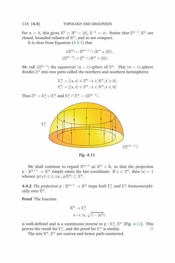
114 [4.4] TOPOLOGY AND GROUPOIDS
For n = 0, this gives E0 = B0 = {0}, S−1 = ∅. Notice that Sn−1,En areclosed, bounded subsets of Rn, and so are compact.
It is clear from Equation (4.4.1) that
i[En] = En+1 ∩ (Rn × {0}),
i[Sn−1] = Sn ∩ (Rn × {0}).
We call i[Sn−1] the equatorial (n − 1)-sphere of Sn. This (n − 1)-spheredivides Sn into two parts called the northern and southern hemispheres
En+ = {(x, t) ∈ Sn : x ∈ Rn, t > 0},
En− = {(x, t) ∈ Sn : x ∈ Rn, t 6 0}.
Thus Sn = En+ ∪ En− and En+ ∩ En− = i[Sn−1].
En+
i[S(n−1)]
Fig. 4.11
We shall continue to regard Rn+1 as Rn × R, so that the projectionp : Rn+1 → Rn simply omits the last coordinate. If x ∈ Sn, then |x| = 1
whence |p(x)| 6 1, i.e., p[Sn] ⊆ En.
4.4.2 The projection p : Rn+1 → Rn maps both En+ and En− homeomorphi-
cally onto En.
Proof The function
En → En+
x 7→ (x,√1− |x|2)
is well-defined and is a continuous inverse to p | En+,En [Fig. 4.11]. This
proves the result for En+, and the proof for En− is similar. ✷
The sets Bn,En are convex and hence path-connected.

IDENTIFICATION SPACES AND CELL COMPLEXES [4.4] 115
4.4.3 Sn is path-connected for n > 1.
Proof From 4.4.2, En+,En− are path-connected. But En+ ∩ En− is non-empty
for n > 1, and so Sn is path-connected by 3.4.2. ✷
There is an important connection between cells, spheres, and the coneconstruction. We recall that for any topological space X, the cone on X is
CX = X× I/X× {0}.
4.4.4 There is a homeomorphism h : CSn−1 → En.
Proof The function
k : Sn−1 × I→ En
(x, t) 7→ tx
is continuous and surjective. Since all the spaces concerned are compactand Hausdorff, k is an identification map. Also k shrinks Sn−1 × {0} to thepoint 0 of En. It follows that k defines a homeomorphism h : CSn−1 → En.
✷
For any space X, let the suspension of X be
SX = CX/X× {1}.
Thus SX is obtained from X× I by shrinking to a point first X× {0} and thenX× {1}. Let l be the composite of the identification maps X×I→ CX→ SX;by 4.2.5, l is an identification map.
The picture for SX is Fig. 4.12 in which each section X × {t}, t 6= 0, 1
is homeomorphic to X under the projection X × {t} → X. The subspacesX × [ 1
2, 1], X × [0, 1
2] are mapped by l to subspaces C+X,C−X. By an easy
application of (d) of 4.3.1 (Corollary 1), l restricts to an identification mapX× [0, 1
2]→ C−X and so we have an identification map
X× I→ X× [0, 12]→ C−X
(x, t) 7→ (x, t/2) 7→ l(x, t/2)

116 [4.4] TOPOLOGY AND GROUPOIDSr+
r−
C+X
C−X
X× { 12}
Fig. 4.12
which shrinks to a point X× {0}. It follows that there is a homeomorphismCX → C−X. A similar argument (using the homeomorphism I → [ 1
2, 1]
given by t 7→ 1 − t/2) shows that there is a homeomorphism CX → C+X;on X× {1} both of these homeomorphisms send (x, 1) 7→ (x, 1
2).
The argument of the last paragraph generalises the representation of Sn
as the union of its Northern and Southern hemispheres. In fact, by the lastparagraph, 4.4.2, and 4.4.4, we can construct the homeomorphisms
En+ → C+Sn−1, En− → C−Sn−1
which on i[Sn−1] are given by (x, 0) 7→ (x, 12). By the gluing rule for home-
omorphisms [2.7.3] these homeomorphisms define a homeomorphism
Sn → SSn−1.
The composite
En h−1
−→ CSn−1 p−→ SSn−1
(where p is the identification map) is injective on Bn and shrinks theboundary Sn−1 of En to a point. It follows that En/Sn−1 is homeomor-phic to SSn−1, and hence there is a homeomorphism
k : En/Sn−1 → Sn.
This homeomorphism sends the shrunken Sn−1 to the South Pole P =
(0, . . . , 0,−1) of Sn. Further, Bn is a subspace of En/Sn−1 and k maps Bn

IDENTIFICATION SPACES AND CELL COMPLEXES [4.4] 117
homeomorphically onto Sn \ {P}. For this reason, we write
Sn = e0 ∪ en
where er denotes an open r-cell, or r-ball, that is, a space homeomorphic toBr. In the case of Sn, e0 = {P}, en = Sn \ {P}.
It might be expected that Sn \ {x} is homeomorphic to Bn for any pointx of Sn. This is in fact true, and is a consequence of the homogeneity of Sn
by which is meant that for any points x,y of Sn there is a homeomorphismσ : Sn → Sn such that σ(x) = y [cf. Exercise 5 of Section 5.4].
We conclude this section by proving a simple result which will have amore general analysis in chapter 5.
4.4.5 There is a homeomorphism Em × En → Em+n.
Proof Let ‖ ‖ denote the Cartesian norm on Rn and let
Jn = {x ∈ Rn : ‖x‖ 6 1}.
Thus Jn is the n-fold product of the interval [−1, 1] with itself. The associa-tivity of the product shows that Jm× Jn is homeomorphic to Jm+n. So ourresult is proved if we exhibit a homeomorphism from Em to Jm.
Consider the function
f : Em → Jm
x 7→{‖x‖−1|x|x, x 6= 0
0, x = 0.
Then f is a bijection, and is continuous certainly at all x 6= 0. We prove f iscontinuous at 0.
The closed ball about 0 of radius r in the Euclidean norm is rEm, and inthe Cartesian norm is rJm. Also
f−1[rJm] = rEm
But the sets rEm, and also the sets rJm, taken for all r > 0 form bases forthe neighbourhoods of 0. Therefore, f is continuous at 0.
A similar argument shows that f−1 is continuous. ✷
Now Ei is a subset of Ri, i = m,n,m+n, so that Em×En is a subset ofRm+n. Let ‘interior’ mean the interior operator on these Euclidean spaces.Then the homeomorphism h : Em × En → Em+n constructed above mapsthe interior of Em × En bijectively onto the interior of Em+n, that is, itmaps Bm × Bn bijectively onto Bm+n. Therefore, h maps the boundary

118 [4.5] TOPOLOGY AND GROUPOIDS
of Em × En bijectively onto the boundary of Em+n; hence h restricts to ahomeomorphism
Sm−1 × En ∪ Em × Sn−1 → Sm+n−1. (4.4.6)
EXERCISES
1. Let x0 ∈ Sn and let Π be the hyperplane in Rn+1 which is perpendicular to x0and which passes through the origin. Let s : Sn \ {x0} → Π be the stereographic
projection defined as follows: if x ∈ Sn \ {x0} then s(x) is the unique point of Π such
that s(x), x, and x0 are collinear. Let p : Rn+1 → Π be the perpendicular projection
onto Π. Prove that for each x ∈ Sn \ {x0}
s(x) = p(x)/(1 − cos θ)
where θ is the angle between x and x0. Prove also that s is a homeomorphism.
2. Prove that En+ is a retract of Sn. Prove also that each point x of Sn has a base B
for the neighbourhoods (in Sn) of x such that each element of B is a retract of Sn.
3. Let the points of Rp+q+2 be denoted by (x, y) where x ∈ Rp+1, y ∈ Rq+1. Define
subsets A+,A− of Sp+q+1 by
A+ = {(x,y) ∈ Sp+q+1 : |x| > |y|},
A− = {(x,y) ∈ Sp+q+1 : |x| 6 |y|}.
Prove that A+ is homeomorphic to Sp × Eq+1, A− is homeomorphic to Ep+1 × Sq,
and A+ ∩A− is homeomorphic to Sp × Sq.
4. Let X be a topological space and let x0 ∈ X. Define the reduced cone and reduced
suspension respectively by
ΓX = X× I/(X× {0} ∪ {x0}× I),
ΣX = X× I/(X× {0, 1} ∪ {x0}× I).
Prove that ΓSn−1 is homeomorphic to En, and that ΣSn−1 is homeomorphic to Sn.
4.5 Adjunction spaces
Arbitrary identification spaces are so general that it is difficult to say any-thing about them. We therefore concentrate attention on a special kind ofidentification space—the adjunction spaces—which occur commonly andfor which we can prove useful theorems.
Suppose there is given a topological space X, a closed subspace A of Xand a map f : A→ B. The adjunction space
B f⊔ X

IDENTIFICATION SPACES AND CELL COMPLEXES [4.5] 119
is obtained by ‘gluing’ X to B by means of f. More precisely, we have arelation from X to B given by
x ∼ b⇔ x ∈ A and fx = b.
The elements of B f⊔ X are then the equivalence classes of B⊔X under theequivalence relation generated by ∼.
Let F : B ⊔ X→ B f⊔ X be the projection. We have a diagram
Af //
i
��
B
i
��X
f// B f⊔ X
(4.5.1)
in which i is the inclusion and i, f are composites
Bi1 // B ⊔ X F // B f⊔ X, X
i2 // B ⊔ X F // B f⊔ X.
Clearly, diagram (4.5.1) is commutative, that is, fi = if, since if a ∈ Ai2(a) ∼ i1f(a) in B ⊔ X.
An equivalence class of B ⊔ X either contains a single element i2(x) forx in X \A or is {i1(b)}∪ i2f−1[b] for b in B. It is usual, therefore, to identifyx in X \A and b in B with their corresponding equivalence classes in B⊔X,and so to regard B f⊔ X as the union of the sets B and X\A. This conventioncauses confusion only when B meets X \A.
The topology on B f⊔ X is to be the final topology with respect to i, f or,equivalently, the identification topology with respect to
F : B ⊔ X→ B f⊔ X.If g : B f⊔ X → Y is any map, then we can construct a commutative
diagram of maps
Af //
i
��
B
i ′
��X
f ′// Y
(4.5.2)
where i ′ = gi, f ′ = gf. The converse of this statement gives a method ofconstructing maps from B f⊔ X to Y.

120 [4.5] TOPOLOGY AND GROUPOIDS
4.5.3 If i ′ : B → Y, f ′ : X → Y are maps such that f ′i = i ′f, then there is aunique map g : B f⊔ X→ Y such that
gi = i ′, gf = f ′.
Proof Let x ∈ X, b ∈ B. The condition f ′i = i ′f ensures that
x ∼ b⇒ f ′(x) = i ′(b).
The result is immediate from Example 1 of Section 4.2. ✷
In the usual way, the ‘universal’ property 4.5.3 characterises i, f up to ahomeomorphism—if the maps f ′, i ′ of diagram (4.5.2) are universal thenthe map g : B f⊔ X→ Y of 4.5.3 is a homeomorphism. This type of universalproperty occurs in diverse situations and so deserves a name. Suppose weare given a commutative diagram of maps of topological spaces
X0
i1 //
i2
��
X1
u1
��X2 u2
// X
(4.5.4)
Then we say (u1,u2) is a pushout of (i1, i2), and also that the square (4.5.4)is a pushout, if the following property holds: if u′
1 : X1 → X′, u′2 : X2 → X′
are maps such that u′1i1 = u′
2i2, then there is a unique map u : X → X′
such that uu1 = u′1, uu2 = u′
2. As usual, this property characterises thepair (u1,u2) up to a homeomorphism of X. For this reason, it is commonto make an abuse of language and refer to X as the pushout of (i1, i2). Insuch case, we write
X = X1 i1⊔ i2 X2.
(In chapter 7 we shall need the notion of a weak pushout: the definitionof this is the same as that of pushout except that the word unique is omitted.Of course, the property that (4.5.4) is a weak pushout does not characterise(u1,u2) up to a homeomorphism of X.)
We shall, as above, restrict the term adjunction space to a pushout of apair (f, i) in which i is an inclusion of a closed subspace; and, of course, weare abbreviating B f⊔ i X to B f⊔ X. The map f is called the attaching map
of the adjunction space.
One of the good features of adjunction spaces is shown in the followingresult.

IDENTIFICATION SPACES AND CELL COMPLEXES [4.5] 121
4.5.5 (a) i is a closed map. (b) f | X \A is an open map.
Proof (a) Let C be closed in B and let C′ = i[C]. Then
i−1[C′] = C, f−1[C′] = f−1[C].
The first set is closed in B (trivially) and the second set is closed in X be-cause f is continuous and A is closed in X. Since B f⊔ X has the finaltopology with respect to i, f, it follows from 4.2.2(b) that C′ is closed inB f⊔ X.(b) Let U be open in X \ A and let U ′ = f[U]. Then
i−1[U ′] = ∅, f−1[U ′] = U.
These sets are open in B,X respectively, and so U ′ is open in B f⊔ X. ✷
It is immediate from 4.5.5 that i is a homeomorphism onto a closedsubspace, and f | X \ A is a homeomorphism onto an open subspace ofB f⊔ X. So if we identify B and X \ A with the corresponding subsets ofB f⊔ X, we obtain:
4.5.5 (Corollary 1) B is a closed subspace, and X \ A is an open subspace, of
B f⊔ X.
In some cases, adjunction spaces can be regarded as identificationspaces.
4.5.6 If f : A→ B is an identification map, then so also is f : X→ B f⊔ X.
Proof Clearly f is surjective. We prove that B f⊔ X has the final topologywith respect to f. Suppose g : B f⊔ X → Y is such that gf : X → Y iscontinuous. Then gfi = gif is continuous. Since f is an identification map,the continuity of gif implies the continuity of gi. Finally, the continuity ofgf and gi implies the continuity of g. ✷

122 [4.5] TOPOLOGY AND GROUPOIDS
EXAMPLES
1. If A is empty, then B f⊔ X = B⊔X. If A = X, then B f⊔ X = B. If A = B,then B 1⊔ X = X.2. Suppose X = B∪C, A = B∩C where B,C are closed in X. Let j : A→ B
be the inclusion. Then
X = B j⊔ C.
The only problem here is one of topology; the fact that X has the finaltopology with respect to the inclusions B → X, C → X is a consequence ofthe Gluing Rule [2.5.12].3. Let B be the space consisting of a single point b, let A be non-empty, andlet f : A → B be the unique map. Clearly, f is an identification map, andtherefore so also is f : X → B f⊔ X. Since f simply shrinks A to a point itfollows that B f⊔ X is homeomorphic to X/A; the only difference betweenthese spaces is that in B f⊔ X the point A of X/A has been replaced by b.4. Many common identification spaces can be regarded as adjunctionspaces. For example, let A1,A2 be closed in X and let ϕ : A1 → A2 bea homeomorphism which is the identity on A1 ∩A2. Let f : A1 ∪A2 → A2
be the identity on A2 and ϕ on A1—the given conditions ensure that f iswell-defined and continuous. Let Y = A2 f⊔ X. It is easy to prove that f isan identification map, and it follows that f : X→ Y is an identification map.Thus Y is obtained from X by the identifications a1 ∼ ϕa1 for all a1 ∈ A1.5. One of our principal examples of adjunction spaces is when X = En,the standard n-cell, and A = Sn−1, the standard (n − 1)-sphere. Thus, letn = 1. Then E1 = [−1, 1], S0 = {−1,+1} and B f⊔ En can be pictured asone of the spaces in Fig. 4.13.
B B
Fig. 4.13
For n > 1, and even for n = 2, it is usually impossible to visualiseB f⊔ En. But some special cases are of interest. First of all let B consist ofa single point: B f⊔ En is homeomorphic to En/Sn−1 which, as we haveseen in section 4.4, is homeomorphic to Sn.
Second, consider the function
f : S1 → B
z 7→ Re(z)

IDENTIFICATION SPACES AND CELL COMPLEXES [4.5] 123
where B = [−1, 1]. Then B f⊔ E2 is homeomorphic to S1. The picture forthis is Fig. 4.14 (which may be thought of as illustrating the operation ofzipping up a purse).
Fig. 4.14
Third, let f : S1 → S1 be the function z 7→ z2. Then f identifies thepoints ±z for z in S1 and f is an identification map. Therefore S1 f⊔ E2 ishomeomorphic to S2 with antipodal points identified. This space is a modelof the real projective plane P2(R) of chapter 5.6. A pointed space is a topological space X and a point x0 of X, called thebase point such that {x0} is closed in X. Let X, Y be pointed spaces. Thewedge of X and Y is the space X ∨ Y obtained from X and Y by identifyingx0 with y0. Fig. 4.15 illustrates S1 ∨ S2 (for some choice of base points)and S2 ∨ S2 can be thought of as two tangential 2-spheres in R3.
Fig. 4.15
If we take the boundary of a square and identify opposite sides accord-ing to the schemes of either Fig. 4.3 or Fig. 4.4 on p. 98, then the result isessentially S1 ∨ S1.7. Let T2 be the torus and let g : I2 → T2 be the identification map by whichopposite edges of I2 are identified. Let h : E2 → I2 be a homeomorphismwhich maps S1 onto the boundary of I2 (in fact any homeomorphism E2 →I2 does this), and let f = gh : E2 → T2. Then f[S1] is essentially a subsetS1 ∨ S1 of T2 (the the last example). Since f is an identification map wecan say that T2 is homeomorphic to (S1 ∨ S1) f⊔ E2 where f is a mapS1 → S1 ∨ S1.
We have shown how to construct spaces using adjunction spaces. On

124 [4.5] TOPOLOGY AND GROUPOIDS
the other hand, it may help us to grasp the topology of a given space Q ifwe can represent Q as an adjunction space or, at least, a homeomorph ofB f⊔ X. This can give a ‘structure’ to the spaceQ, in showing how it is madeup from smaller and often better understood pieces put together in a welldefined way. Further, by 4.5.3, we then know how to construct continuousfunctions on Q in terms of continuous functions on these smaller pieces Band X. We will see that constructing particular mathematical structures aspushouts occurs widely in mathematics.
Suppose there is given then a closed subspace B ofQ, a closed subspaceA of X and a map f ′ : X→ Q such that f ′[A] ⊆ B. Consider the diagram
Af //
i
��
B
i ′
��X
f ′// Q
(4.5.7)
in which i, i ′ are the given inclusions, and f is the restriction of f ′. We thenask for conditions which ensure that (4.5.7) is a pushout.
Suppose (4.5.7) is a pushout of spaces and maps. Then there is a home-omorphism k : Q → B f⊔ X such that kf ′ = f, ki ′ = i. Because of theconstruction of B f⊔ X it follows that h = f ′ | X\A,Q\B is a bijection. Also,
if this map h is a bijection, then (4.5.7) is a pushout of sets—if f : X → Y,
i : B → Y are functions such that fi = if, then there is a unique function
g : Q→ Y such that gi ′ = i, gf ′ = f, where g is i on B and x 7→ fh−1(x) onQ \ B.
Suppose then h = f ′ | X \A,Q \B is a bijection and, as before, that B isclosed in Q, A is closed in X.
4.5.8 The square (4.5.7) is a pushout if f ′[X] is closed in Q and f ′ | X, f ′[X]is an identification map. These conditions hold if X is compact and Q is
Hausdorff.
Proof The last statement is clear. For the first statement, we have to provethat Q has the final topology with respect to i ′, f ′.
Let C be a subset of Q such that i ′−1[C], f ′−1[C] are closed in B,X re-spectively. Then B ∩ C = i ′−1[C] is closed in B and hence is closed in Q.Also if
C′ = C ∩ f ′[X] = f ′f ′−1[C],

IDENTIFICATION SPACES AND CELL COMPLEXES [4.5] 125
then C′ is closed in f ′[X] (since f ′ | X, f ′[X] is an identification map) andtherefore C′ is closed in Q). Therefore
C = (B ∩ C) ∪ C′
is closed in Q. ✷
We shall need the notion of attaching a number of spaces: this is asimple extension of previous results, so we sketch the theory, leaving thedetails as exercises.
Let B be a topological space, let (Xλ)λ∈Λ be a family of spaces, and foreach λ in Λ let Aλ be a closed subset of Xλ and let fλ : Aλ → B be a map.The adjunction space
Q = B (fλ)⊔ (Xλ)
is obtained by identifying each aλ of Aλ with fλ(aλ) in B. Thus Q is anidentification space of the sum of B and all the Xλ. Providing the Xλ aredisjoint and do not meet B, the underlying set of Q can be identified withthe union of B and all the Xλ\Aλ. There is an inclusion i : B→ Q, and thereare maps fλ : Xλ → Q. The topology of Q is the final topology with respectto the family consisting of i and all fλ. The maps i and fλ | Xλ \ Aλ areclosed and open maps respectively. The adjunction spaceQ is characterisedby the universal property: if iλ : Aλ → Xλ is the inclusion, and i ′ : B → Y,gλ : Xλ → Y are maps such that gλiλ = i ′fλ, λ ∈ Λ, then there is a uniquemap g : Q → Y such that gi = i ′, gfλ = gλ, λ ∈ Λ. In the case Λ is finite,say Λ = {1, . . . ,n}, we write
Q = B f1⊔ X1 · · · fn⊔ Xn.
This notation is unambiguous since fi is a map to B.
EXERCISES
1. LetQ be the subspace of R2 which is the union of {0}× [0, 2] and the set {(x,y) ∈R2 : 0 < x 6 1/π, sin 1/x 6 y 6 2}. Let B be the boundary of the subset Q of R2.
Prove that B is closed in Q, that Q \ B is homeomorphic to B2, but that Q is not
homeomorphic to B f⊔ E2 for any f : S1 → B.
2. Let B be a topological space and let fλ : Aλ → B be maps, where Aλ is a closed
subset of Xλ and λ = 1, 2. Let i1 : B → B f1⊔ X1 be the inclusion. Characterise the
adjunction space
Q ′ = (B f1⊔ X1) if2⊔ X2
by a universal property and prove that Q ′ is homeomorphic to B f1⊔ X1 f2⊔ X2.
Generalise this result to arbitrary finite indexed families (fλ), (Xλ).

126 [4.6] TOPOLOGY AND GROUPOIDS
3. Let B be a closed subspace of Q. For each λ = 1, . . . ,n let fλ : Xλ → Q be a map,
and let Aλ be a closed subspace of Xλ such that (i) fλ[Aλ] ⊆ B, (ii) fλ | Xλ \ Aλ is
injective, (ii) the sets fλ[Xλ \Aλ] are disjoint and cover Q \ B, (iv) fλ | Xλ, fλ[Xλ] is
an identification map. Prove that a function g : Q → Y is continuous if and only if
g | B, gfλ is continuous, λ = 1, . . . ,n. Prove also that there is a homeomorphism
Q→ B f1⊔ X1 · · · fn⊔ Xn
which is the identity on B.
4. Let B f⊔ X be an adjunction space, where f : A → B. Prove that B is a retract
(see p. 127) of B f⊔ X if and only if there is a map g : X → B such that g | A = f.
Deduce that if A is a retract of X then B is a retract of B f⊔ X.
4.6 Properties of adjunction spaces
Throughout this section we suppose given an adjunction space B f⊔ X andthe pushout square
Af //
i
��
B
i
��X
f// B f⊔ X
Let F : B ⊔ X→ B f⊔ X be the identification map.
4.6.1 Let B′,X′ be subspaces of B,X respectively such that X′ ⊇ A and B′ ⊇f[A]. Let g = f | A,B′. Then B′
g⊔ X′ is a subspace of B f⊔ X.
Proof We have to prove that the restriction of F
F′ : B′ ⊔ X′ → F[B′ ⊔ X′]
is an identification map, and for this we can use 4.3.1.Notice that F is injective on (B \B′)⊔ (X \X′). Suppose that U ⊆ B⊔ X
and U ′ = U ∩ (B′ ⊔ X′). Then U is F-saturated⇔ U ′ is F′-saturated (sinceall the identifications take place in B′ ⊔ X′). So 4.3.1 applies, and F′ is anidentification map. ✷
We now consider the connectivity of B f⊔ X.
4.6.2 If A is non-empty and X and B are connected then B f⊔ X is connected.
Proof The space B f⊔ X is the union of the sets B and f[X] both of whichare connected. But B meets f[X] (since A is non-empty); therefore B f⊔ Xis connected [3.2.5]. ✷

IDENTIFICATION SPACES AND CELL COMPLEXES [4.6] 127
4.6.3 If A is non-empty and X and B are path-connected then B f⊔ X ispath-connected.
The proof of 4.6.3 is similar to that of 4.6.2.
4.6.4 If B f⊔ X and A are connected then B is connected.
Proof Suppose that B is not connected and that i ′ : B → Y is a map ontothe discrete space Y = {1, 2}. Since A is connected, i ′f : A → Y is constantwith value 1 say. Let f ′ : X→ Y be the constant function with value 1. Theni ′f = f ′i.
By the pushout property 4.5.3, there is a map g : B f⊔ X→ Y such thatgf = f ′, gi = i ′. The last condition shows that g is surjective; hence B f⊔ Xis not connected. ✷
If B,X are compact then so also is the sum B ⊔ X and hence B f⊔ X iscompact.
The question of whether B f⊔ X is Hausdorff is important but ratherdelicate. It is true that if B and X are normal then so also is B f⊔ X [cf.Exercise 6 and also [Hu64]]. We shall prove not this but instead a resultinvolving the placing of A in X which is satisfied in many cases [cf. Section7.3].
We recall that a retraction of X onto A is a map r : X → A such thatr | A is the identity. If such a retraction exists we say A is a retract of X. Toprove that A is a retract of X it is of course sufficient to produce a retractionX→ A—it is rather harder to prove that A is not a retract of X. A retractionX → A is surjective: so A is not a retract of X if X is connected and A isnot connected. For example, S0 is not a retract of E1. We shall later be ableto prove that S1 is not a retract of E2; the proof that Sn is not a retract ofEn+1 for any n is beyond the scope of this book.
We say A is a neighbourhood retract of X if A is a retract of some neigh-bourhood of A in X. This neighbourhood may always be taken to be takento be open since, if A ⊆ IntN and r : N→ A is a retraction, then so also isr | IntN.
EXAMPLES
1. A space X is a retract of itself. If x ∈ X then {x} is a retract of X. Theproduct of retractions is a retraction; hence for any Y, {x}× Y is a retract ofX× Y.2. Sn is a neighbourhood retract of En+1 since the map
En+1 \ {0}→ Sn
x 7→ x/|x|
is a retraction.

128 [4.6] TOPOLOGY AND GROUPOIDS
3. L is not a neighbourhood retract of I. For supposeN is a neighbourhoodof L in I and r : N → L is continuous. For some ε > 0, N contains[0, ε], which is connected. Hence r is constant on [0, ε] and so cannot be aretraction.
4.6.5 The adjunction space B f⊔ X is Hausdorff if the following conditions
hold:
(a) B and X are Hausdorff,
(b) Each x ∈ X \ A has a neighbourhood closed in X and not meeting A,
(c) A is a neighbourhood retract of X.
Proof Let Q = B f⊔ X and let y1,y2 ∈ Q. In order to find disjoint neigh-bourhoods W1,W2 of y1,y2, we distinguish three cases.
(i) Suppose y1,y2 ∈ X \ A. Since X \ A is Hausdorff there are disjoint setsW1,W2 which are neighbourhoods in X\A of y1,y2. But X\A is open in Q[4.5.5 (Corollary 1)]. So W1,W2 are also neighbourhoods in Q of y1,y2.(ii) Suppose y1 ∈ X \ A, y2 ∈ B. Let W1 be a neighbourhood of y1 closedin X and not meeting A. Then W1 is also a neighbourhood in Q of y1.
Let W2 = Q \W1. Then
i−1i[W2] = B, f−1[W2] = X \W1
which are open in B,X respectively. Hence W2 is open in Q.(iii) Suppose y1,y2 ∈ B. Since B is Hausdorff there are in B disjoint openneighbourhoods V1,V2 of y1,y2. Then f−1[V1], f
−1[V2] are open in A, butnot necessarily open in X. We therefore use the neighbourhood retractionto enlarge them into sets open in X.
Let r : N→ A be a retraction where N is open in X. Let
V ′i = r
−1f−1[Vi], i = 1, 2.
Then V ′1,V
′2 are disjoint open sets open in N and so open in X. Notice also
that because r is a retraction
V ′i \A = V ′
i \ f−1[Vi], i = 1, 2.
Let Wi be the subset of Q
Wi = Vi ∪ (V ′i \A), i = 1, 2.
Then i−1[Wi] = Vi, and
f−1[Wi] = f−1[Vi] ∪ (V ′
i \A)
= V ′i .

IDENTIFICATION SPACES AND CELL COMPLEXES [4.6] 129
ThereforeWi is open in Q. Clearly, y1 ∈W1, y2 ∈W2. ✷
(The existence, for each A closed in X and each x ∈ X \ A , of a closedneighbourhood of x not meeting A is one of the standard separation ax-ioms. Such a space X is called T3 by [Bou66], who also calls X regular if itis T3 and Hausdorff. The opposite terminology is used by [Kel55].)
EXAMPLES
4. If X is a metric space and A is closed in X then condition (b) of 4.6.5is always satisfied. For suppose x ∈ X \ A; then dist(x,A) = ε > 0 [2.9.2]and E(x, ε/2) is a closed neighbourhood of x not meeting A. The conditionis also satisfied if X is Hausdorff and A is compact [3.5.6 (Corollary 3)]. Iffollows (for either reason!) that, if f : Sn−1 → B and B is Hausdorff, thenB f⊔ En is Hausdorff.5. Let X, Y be topological spaces and let f : X → Y be a map. Let f ′ :
X× {0}→ Y be the map (x, 0) 7→ f(x). Since X× {0} is a closed subspace ofX× I we can define the adjunction space [Fig. 4.16]
M(f) = Y f′⊔ (X× I).
Y
X× {1}
Fig. 4.16
This is the mapping cylinder of f. It is a construction of great use in chapter7. If X is Hausdorff, then so also is X× I. It is easy to verify the conditions(b) and (c) of 4.6.5 with A,X replaced by X× {0}, X× I. Hence, if X and Y
are Hausdorff, then so also is M(f).
The mapping cone of f is
C(f) =M(f)/X× {1}.
We can prove by a similar method that if X and Y are Hausdorff, then soalso is C(f).

130 [4.6] TOPOLOGY AND GROUPOIDS
Our next result will become vital when we come to consider homotopiesof maps of adjunction spaces in chapters 7 and 9.
4.6.6 Let Y be a locally compact space. In the following diagrams let the first
square be a pushout; then the second square is a pushout.
Af //
i
��
B
i
��X
f// Q
A× Y f× 1 //
i× 1
��
B× Y
i× 1
��X× Y
f× 1// Q× Y
Proof As sets, Q = B⊔ (X \A), Q×Y = (B×Y)⊔ (X \A)×Y. So the onlyproblem is the topology on Q×Y. But since the map F : B⊔ X→ Q definedby i, f is an identification map, so also is F × 1 : (B ⊔ X) × Y → Q × Y, by4.3.2. This completes the proof. ✷
The main utility of this result is that to specify a map Q × Y → Z it issufficient to give a commutative diagram
A× Y f× 1 //
i× 1
��
B× Y
j
��X× Y
g// Z
For further properties of adjunction spaces we refer the reader to §3 ofchapter IV of [Hu64] and also to [Mic66].
EXERCISES
1. Prove that the adjunction space B f⊔ X is a T1-space if B and X are T1-spaces.
2. Let X be a non-normal space. Prove that there are disjoint, closed subsets A,B
of X such that (X/A)/B is not Hausdorff.
3. Prove that R/Z does not satisfy the first axiom of countability.
4. Prove the following generalisation of 4.6.5: an adjunction space B (fλ)⊔ (Xλ)
is Hausdorff if for each λ in Λ (i) B and Xλ are Hausdorff, (ii) each x in Xλ \ Aλ
has a neighbourhood closed in Xλ and not meeting Aλ, (iii) Aλ is a neighbourhood
retract of Xλ.

IDENTIFICATION SPACES AND CELL COMPLEXES [4.7] 131
5. Let X, Y be spaces and let x0 ∈ X, y0 ∈ Y. Prove that if P is the subspace
X× {y0} ∪ {x0}× Y of X× Y then the square of inclusions
{(x0,y0)} //
��
{x0}× Y
��X× {y0} // P
is a pushout square. Deduce that if x0,y0 are taken as base points of X,Y respec-
tively, then P is homeomorphic to X∨ Y.
6. Prove that an adjunction space B f⊔ X is normal if B and X are normal. Give an
example showing the converse is false. [Assume the Tietze Extension Theorem.]
7. Let the space X be the union of a family (Xi)i∈N of subspaces such that (i) for
each i ∈ N, Xi is a closed subset of Xi+1, (ii) a set C is closed in X if and only if
C ∩ Xi is closed in Xi for each i in N. Prove that if each Xi is a normal space, then
so also is X. [Assume the Tietze Extension Theorem.]
8. Let A be a closed subspace of X, and let f : A → B, g : B → C be maps. Prove
that the spaces
C g⊔ (B f⊔ X), C gf⊔X
are homeomorphic.
9. Let i : A→ X, j : X → Y be inclusions of closed subspaces, and let f : A → B be
a map. Prove that the spaces
B f⊔ Y, (B f⊔ X) f⊔ Y
are homeomorphic.
10. Let A be a closed subspace of X and f : A→ B a map. Prove that the subspace
L = (B f⊔ X) × {0} ∪ B × I of M = (B f⊔ X) × I is homeomorphic to (B × I) f×1⊔(X× {0} ∪A× I), where f× 1 : A× I→ B× I. Hence show that if X× {0} ∪A× I is
a retract of X× I, then L is a retract of M.
4.7 Cell complexes
In order to emphasise the intuitive ideas, we shall restrict ourselves to finitecell complexes. Indeed the theory for infinite cell complexes involves, in themain, arranging the topologies so that theorems and proofs for the finitecase carry over almost without change to the infinite case.
There are two useful ways of thinking about cell complexes: (a) con-structive, (b) descriptive. In the first approach, we simply construct cellcomplexes by starting in dimension −1 with the empty set ∅, and then at-tach cells to ∅ in order of increasing dimension. In the second approach,we suppose there is given a topological space X, and seek to describe X in

132 [4.7] TOPOLOGY AND GROUPOIDS
a useful way as the union of open cells. In both approaches, a vital role isplayed by the sequence of skeletons, the n-skeleton being the union of allcells of dimension 6 n.
The constructive approach
We construct a sequence of spaces Kn such that Kn ⊆ Kn+1, n > −1. Thespace K−1 is to be the empty set. Suppose that Kn−1 has been constructed.We suppose given maps
fn1 , . . . , fnrn
: Sn−1 → Kn−1.
Then Kn is to be the adjunction space
Kn−1fn1⊔ En · · · fnrn⊔ En.
For n > 0, we allow the case r = 0, when Kn = Kn−1. In fact, since weare dealing only with finite cell complexes, we shall assume that for someN, Kn = Kn−1 for n > N, and define K = KN. Note that if K0 is empty, soalso is K.
Let us consider the intuitive picture, in low dimensions, of a non-emptycell complex. The 0-skeleton K0 is a non-empty, finite, discrete space. The1-skeleton K1 is formed by attaching to K0 a finite number (possibly 0) of1-cells by means of maps f11, . . . , f
1r1
: S0 → K0. Now S0 is the discrete space{−1,+1}. So for each i = 1, . . . , r1 the map f1i is either constant or maps totwo distinct points of K0. Thus a representative picture for K1 is Fig. 4.17,where the dots denote elements of K0.
Fig. 4.17
Next we form K2 by attaching a finite number of 2-cells to K1 by meansof maps f21, . . . , f
2r2
: S1 → K1. It can be shown that if K1 has 1-cells (i.e., ifK1 6= K0) then there is an uncountable number of maps S1 → K1. It is evenpossible to construct an uncountable set of spaces of the form I f⊔ E2, notwo of which are homeomorphic.

IDENTIFICATION SPACES AND CELL COMPLEXES [4.7] 133
The pictures in Fig. 4.18 are of two simple cell complexes of the formE1
f⊔ E2, where K0 = {−1,+1}, K1 = E1. In (a), f[S1] = {+1}; in (b),f[S1] = {0}.
(a) (b)Fig. 4.18
It may be felt that, because of the wide latitude in the attaching maps,cell complexes are bizarre spaces, and that the attaching maps should berestricted in some way, for example to be the embeddings. However, manyimportant spaces, for example the projective spaces, have natural cell struc-tures in which the attaching maps are not embeddings. Also we shall beconsidering homotopies of attaching maps in chapter 7 and any restrictionon these maps would be inconvenient.
The burden of this section is that cell complexes are always ‘good’spaces, although additional restrictions on the attaching maps might makethem ‘better’. In any case, by results of the last section, a cell complex isalways a compact, Hausdorff space.
The descriptive approach
We recall that an open n-cell (also called an n-ball) is a space e homeomor-phic to the standard n-ball Bn. The dimension of e is the natural numberdim e = n. However the proof that this dimension is well-defined is non-trivial, and depends on the Invariance of Dimension: if f : Rm → Rn is ahomeomorphism, thenm = n. Since Bn is homeomorphic to Rn, it followsthat if e is homeomorphic to Bm and to Bn then m = n; hence dim e iswell-defined.
An idea which occurred early in topology is that of a decomposition ofa space Q by open cells. In this, Q is given as the union
⋃λ∈Λ eλ, where eλ
is an open nλ-cell and the sets eλ are disjoint.The difficulty has always been what to do with such a decomposition,
since it gives relatively little information on the space Q. For example,the ‘bad’ space Q of Exercise 1 of Section 4.5 has a decomposition withtwo 0-cells, two 1-cells and one 2-cell. The two spaces of Fig. 4.19 havedecompositions with one 0-cell, and two 1-cells. Yet by simple local cutpoint arguments they are not homeomorphic.

134 [4.7] TOPOLOGY AND GROUPOIDS
Fig. 4.19
Let us consider what we are given with a decomposition by open cells,Q =
⋃λ∈Λ eλ. For each λ in Λ, there is a homeomorphism kλ : Bnλ → eλ.
Since dim eλ = nλ is uniquely defined, for each natural number n the n-skeleton of Q is well-defined by
Qn =⋃
nλ6n
eλ.
J. H. C. Whitehead realised that a satisfactory theory could be built byassuming the extra condition that the homeomorphism kλ : Bnλ → eλextends to a map hλ : Enλ → Q such that hλ[Snλ−1] ⊆ Qnλ−1. Thisensures that eλ is part of the adjunction of a closed nλ-cell to Qnλ−1; ittakes us to the situation considered before and, from the technical point ofview, allows proofs by induction on the skeletons.
The last sentence is not quite correct. The reason for this is that ifthe number of cells is infinite then the cells do not uniquely determine thetopology ofQ. For example, anyQ has a decomposition in which each pointof Q is a 0-cell. Therefore we restrict ourselves to the finite case, whichretains the geometric ideas without additional topological difficulties.
It is convenient in defining a cell complex to keep the above maps hλ aspart of the structure. It is also necessary to assume that Q is Hausdorff.
Let Q be a non-empty Hausdorff topological space. A cell structure onQ is a finite set of maps
hλ : Enλ → Q, λ ∈ Λ,
called the characteristic maps. Let
eλ = hλ[Bnλ ].
The n-skeleton of the cell structure is
Qn =⋃
nλ6n
eλ.

IDENTIFICATION SPACES AND CELL COMPLEXES [4.7] 135
Then we require that the characteristic maps satisfy:
CS1 hλ | Bnλ , eλ is a bijection.
CS2 the eλ are disjoint and Q =⋃
λ eλ,
CS3 hλ[Snλ−1] ⊆ Qnλ−1.
A cell complex is a space Q with a cell structure on it. It is usual to denotethe cell complex simply by Q.
The space En is compact and Qn−1 is Hausdorff. Therefore Exercise 3of Section 4.5 implies that Qn is homeomorphic to an adjunction space,
Qn−1f1⊔ En · · · fn⊔ En
where fi is a map Sn−1 → Qn−1. This shows how the present definitionlinks with the constructive approach considered first.
Another easy consequence of the definition is that
eλ = hλ[Enλ ] :
for the continuity of hλ implies that
hλ[Enλ ] = hλ[Bnλ ] ⊆ hλ[Bnλ ];
on the other hand h[Enλ ] is a compact, and hence closed, set containingeλ.
4.7.1 Let Q be a cell complex and g : Q→ X a function to a topological space
X. The following conditions are equivalent.
(a) g is continuous.
(b) ghλ is continuous for each characteristic map hλ.
(c) g | eλ is continuous for each cell eλ.
Proof Obviously (a)⇒ (b) and (a)⇒ (c). Also (c)⇒ (b) since hλ[Enλ ] =
eλ. Since Enλ is compact and Q is Hausdorff, the map hλ | Enλ , eλ is anidentification map.
To complete the proof we show that (b)⇒ (a). The proof is by inductionon the skeletons.
Since Q0 is discrete, g | Q0 is certainly continuous. But if g | Qn−1
is continuous, then by Exercise 3 of Section 4.5 so also is g | Qn. SinceQ = Qn for some n, it follows that g is continuous. ✷
In order to extend the present theory to infinite cell complexes, it isnecessary to take the last result as one of the properties characterising thetopology of Q.

136 [4.7] TOPOLOGY AND GROUPOIDS
The smallest integer n such that Q = Qn is called the dimension of thecell complex Q. The methods which are used to prove the invariance of di-mension can also prove that the dimension of a cell complex is a topologicalinvariant.
Our next result shows one of the ways in which cell complexes are ‘nice’spaces.
4.7.2 If Q is a cell complex, then the following conditions are equivalent.
(a) Q1 is connected,
(b) Q is path-connected,
(c) Q is connected.
Proof Clearly, (b)⇒ (c). We prove also (c)⇒ (a)⇒ (b).
(c) ⇒ (a) The n-sphere Sn is connected for n > 1. Further Qn+1
is homeomorphic to a space obtained by attaching (n + 1)-cells to Qn.Therefore by 4.6.4, if Qn+1 is connected and n > 1, then Qn is connected.But Qn+1 = Q for some n. So the result follows by downward induction.
(a) ⇒ (b) By 4.6.3 and induction on the skeletons, if Q1 is path-connected then so also is Q. So it is sufficient to prove the more generalresult that each path-component of Q1 is both open and closed in Q1.
Let P be a path-component of Q1. If P contains no 1-cells of Q, the Pconsists of an isolated point, which is certainly both open and closed in Q1.We suppose then that P contains more than one point.
A point x of P must belong to e1 for some open cell e1, for otherwise xwould be an isolated point. On the other hand, each e1 is path-connected(since it is the continuous image of E1) and so e1 is either contained in ordisjoint from P. Therefore P is the union of a finite number of e1, and so Pis closed.
We now prove P is open. Let x ∈ P. If x ∈ Q0, then the set N, consistingof x and all open 1-cells e1 such that x ∈ e1, is a path-connected neighbour-hood of x, and so N ⊆ P. If x ∈ Q1 \Q0, then x belongs to some open 1-celle1; clearly e1 is contained in P, and therefore P is a neighbourhood of x. ✷
Let Q be a cell complex with characteristic maps hλ, λ ∈ Λ. Let P be anon-empty subset of Q and let M be the set of λ in Λ such that the imageof hλ is contained in P. For each λ in M, let gλ : Enλ → P be the restrictionof hλ : Enλ → Q. We say P is a subcomplex of Q if the characteristic mapsgλ, λ ∈M, form a cell structure on P. In this case P is covered by the opencells eλ for λ inM and Q\P is covered by the open cells eλ for λ in M\Λ.
EXAMPLES
1. The n-skeleton Qn of Q is a subcomplex of Q.

IDENTIFICATION SPACES AND CELL COMPLEXES [4.7] 137
2. The intersection and the union of a family of subcomplexes of Q areagain subcomplexes of Q.3. Let X be any subset of Q. Then the intersection of all subcomplexes ofQ containing X is the smallest subcomplex of Q containing X.
Let P, R be cell complexes and let f : P → R be a continuous function.We say f is a cellular map if
f[Pn] ⊆ Rn, n > 0.
4.7.3 Let Q,R be cell-complexes, let P be a subcomplex of Q and let f : P → R
be a cellular map. Then the adjunction space R f⊔ Q can be given the structure
of a cell-complex.
Proof The open cells of R f⊔ Q are the open cells of R and ofQ\P. In orderto describe the characteristic maps, let f : Q → R f⊔ Q, i : R → R f⊔ Q bethe usual maps. Let hλ, λ ∈ Λ, be the characteristic maps of Q; gλ, λ ∈M,those of P; and kν,ν ∈ N, those of R. If eν is an open cell of R, then itscharacteristic map in R f⊔ Q is to be ikν. If eλ is an open cell of Q \P, thenits characteristic map in R f⊔ Q is to be fhλ.
The conditions CS1 and CS2 are obviously satisfied, as is CS3 for themaps ikν, ν ∈ N. Since f is cellular, so also is f. Hence CS3 is satisfied forthe maps fhλ, λ ∈ Λ \M. ✷
We now show that the product of cell complexes is a cell complex. LetP,Q be cell complexes with characteristic maps fλ, λ ∈ Λ, gµ, µ ∈ Mrespectively. Since P is the union of disjoint open cells eλ, and Q is theunion of disjoint open cells eµ, P×Q is the union of the disjoint sets eλ×eµ.But eλ × eµ is an open (nλ + nµ)-cell. So the n-skeleton (P ×Q)n is welldefined and
Pm ×Qn ⊆ (P ×Q)m+n.
Suppose that eλ is an open m-cell of P, and eµ is an open n-cell ofQ. Let hmn : Em+n → Em × En be the homeomorphism constructed in4.4.5—we recall that
hmn[Sm+n−1] = Sm−1 × En ∪ Em × Sn−1.
Let kλµ be the composite
Em+n hmn−→ Em × En fλ×gµ−→ P ×Q.
Then kλµ maps Bm+n bijection onto eλ×eµ and kλµ[Sm+n−1] is containedin Pm−1×Qn∪Pm×Qn−1 which is itself contained in (P×Q)m+n−1. Thisshows that the kλµ are characteristic maps for a cell structure on P ×Q.

138 [4.7] TOPOLOGY AND GROUPOIDS
When exhibiting a space as a cell complex it is common practice towrite it simply as the union of open cells, and say afterwards what are thecharacteristic maps. For example, the m-sphere has a cell structure withone m-cell and one 0-cell, and we therefore write
Sm = e0 ∪ em.
Also, if em is an open m-cell of a cell complex Q with characteristic maph : Em → Q, we make an abuse of language and call h | Sm−1,Qm−1 theattaching map of em. In particular, we say that the cell em of Sm is attachedby the constant map.
Consider now Sm × Sn. If we take Sm = e0 ∪ em, Sn = e0 ∪ en, thenwe can write
Sm × Sn = e0 ∪ em ∪ en ∪ em+n.
Here both em and en are attached by constant maps, so that e0 ∪ em ∪ enis homeomorphic to Sm ∨ Sn. Thus Sm × Sn is, up to homeomorphism,(Sm ∨ Sn) ∪ em+n. The attaching maps of the (m + n)-cell is a map w :
Sm+n−1 → Sm ∨ Sn called the Whitehead product map. [cf. Exercise 2 ofSection 5.7 for a generalisation of this map].
EXERCISES
1. Prove that the composite, and product, of cellular maps is cellular. Is the diago-
nal map Q→ Q×Q cellular?
2. Prove that if Q1,Q2 are cell complexes, then so also is Q1 ⊔ Q2.
3. Let Q,R be cell complexes, let i : P → Q be the inclusion of the subcomplex P of
Q, and let f : P → R be cellular. Prove that if K is a cell complex and i ′ : R → K,
f ′ : Q→ K are cellular maps such that i ′f = f ′i, then the unique map g : R f⊔Q→ K
such that gf = f ′, gi = i ′ is cellular.
4. Read an account of the classification of surfaces [for example in [Cai61]] and
give cell structures for the normal forms of surfaces.
The following exercises outline a part of the theory of infinite cell complexes.
5. LetQ be a non-empty, not necessarily Hausdorff, space, and suppose given on Q
a cell structure {hλ}λ∈Λ in the sense of the definition on p. 131 except that Λ is not
supposed finite. We say Q is a CW-complex if the following axioms hold:
CW1 A set C ⊆ Qn is closed in Qn if and only if C ∩Qn−1 is closed in Qn−1 and
h−1λ [C] is closed in En for each λ such that nλ = n.
CW2 A set C ⊆ Q is closed in Q if and only if C ∩Qn is closed in Qn for each n.
Let Λn = {λ ∈ Λ : nλ = n} and let Λn have the discrete topology. Define
q : Qn−1 ⊔ (Λn × En) → Qn to be x 7→ x on Qn−1 and (λ, e) 7→ hλe on Λn × En.
Prove that CW1 is equivalent to: Qn has the identification topology with respect to
q.
In the following exercises, Q denotes a CW-complex with cell structure {hλ}λ∈Λ.

IDENTIFICATION SPACES AND CELL COMPLEXES [4.7] 139
6. Prove that a function f : Qn → Y is continuous if and only if f | Qn−1 is con-
tinuous and fhλ : En → Y is continuous for each λ in Λ with nλ = n. Prove that
a function f : Q → Y is continuous if and only if f | Qn is continuous for each n.
Deduce that f : Q → Y is continuous if and only if fhλ is continuous for each λ in
Λ.
7. Let C be a closed subset of Q and g : C → I any map. Prove that g extends to
a map f : Q → I and thus prove that Q is normal. Prove that each point of Q is
closed, and hence show that Q is Hausdorff. [You may assume the Tietze extension
theorem.]
8. Prove that any compact subset of Q is contained in a finite union of cells eλ. [If
C ⊂ Q meets an infinite number of cells, choose points ci of C, i = 1, 2, . . . , which
lie in distinct cells eλi. Define gci = 1/i and extend g over Q by Exercise 7.]
9. A CW-complex Q is said to be locally finite if each point x of Q has a neighbour-
hood N such that N is contained in a finite subcomplex of Q. Prove that Q is locally
finite if and only if it is, as a topological space, locally compact.
10. Prove that a CW-complex is a k-space. Prove that if P,Q are CW-complexes
then P ×Q, with the cell structure given in the present section, is a CW-complex if
and only if P ×Q is a k-space. Hence show that P ×Q is a CW-complex if P or Q
is locally finite. [Prove first that the weak product space P ×W Q of Exercise 12 of
Section 4.3 is always a CW-complex.]
NOTES
The idea of adjunction space is due to J. H. C. Whitehead, for whom theconcept evolved over a period of about ten years. I heard it said that hetook a year to prove that the product of CW-complexes one of which islocally finite is also a CW-complex. The result 4.6.6 on the product of anidentification map is essentially due to Whitehead.
There are various books which deal with the case of infinite cell com-plexes, that is, CW-complexes. For applications of these complexes in alge-braic topology, see [Spa62] and [Whi78], as well as the basic paper on thetopic, [Whi49].
The fact that 4.6.6 is false without the locally compact assumption leadR. Brown in his thesis ([Bro61]) to suggest Hausdorff k-spaces as an appro-priate tool for topology. See also [Bro63], [Bro64] and section 5.9. Thus4.6.6 gives one indication that the notion of topological space should notbe regarded as the final setting for the concept of continuity.

140 [4.7] TOPOLOGY AND GROUPOIDS

Chapter 5
Projective and other spaces
5.1 Quaternions
In this section, we construct the algebra H of quaternions, and we showthat H is a field. The word field is here used in a slightly more generalsense than is usual, since the multiplication of H is non-commutative. Infact, the term skew field is often used in this context.
As a set, and in fact as a vector space over R, H is just R× R3. Thus, ifq ∈ H then q = (λ, x) where λ is real and x is in R3; we call λ the real part
of q, x the vector part of q and write
Re (q) = λ, Ve (q) = x.
It is convenient to identify (λ, 0) with λ and (0, x) with x, and so to write
q = λ+ x.
We shall, as far as possible, keep this convention of using Greek letters forthe real part, and Roman letters for the vector part, of a quaternion. Thusthe addition and scalar multiplication of the vector space structure of H isgiven by
(λ+ x) + (λ ′ + x ′) = λ+ λ ′ + x+ x ′.
λ ′(λ+ x) = λ ′λ + λ ′x.
We now define a distributive multiplication on H. To do this it suffices todefine the product xy of vectors, since the product of quaternions q = λ+x,r = µ+ y must then, by distributivity, be defined by
qr = λµ+ λy+ µx+ xy (5.1.1)
141

142 [5.1] TOPOLOGY AND GROUPOIDS
However, xy will not be a vector—in terms of the usual scalar and vectorproduct in R3 we set
xy = −x · y+ x× y (5.1.2)
The scalar and vector product of vectors are bilinear. It follows fromthis and (5.1.1), (5.1.2) that multiplication of quaternions is bilinear—thatis, for any quaternions q, r, s and real number λ
q(r + λs) = qr+ λ(qs),
(r+ λs)q = rq+ λ(sq).(5.1.3)
One of the points of definition (5.1.2) is that it replaces the non-associative vector product by an associative product. By well-known rules
x(yz) = x(−y · z + y× z)= −(y · z)x − x · y× z+ x× (y× z)= −x · y× z − (y · z)x+ (x · z)y − (x · y)z
and a similar computation gives the same value for (xy)z. Hence x(yz) =(xy)z. It follows from this and (5.1.1) that for any quaternions q, r, s
q(rs) = (qr)s;
that is, multiplication of quaternions is associative.A vector a of R3 is a unit vector if a · a = 1; this is clearly equivalent to
a2 = −1. Two vectors a,b are orthogonal, that is a · b = 0, if and only ifab is a vector. In such case
ab = a× b = −b× a = −ba.
Conversely, if ab = −ba, then by (5.1.2) a · b = 0 and so a and b areorthogonal.
The ordered set a,b, c of vectors is said to form a right-handed or-
thonormal system if a,b, c are of unit length, are mutually orthogonal, anda× b = c.
5.1.4 The set of vectors a,b, c is a right-handed orthonormal system if and
only if
(a) a2 = b2 = c2 = −1,
(b) abc = −1.
Proof Condition (a) holds if and only if a,b, c are of unit length. If furthera,b are orthogonal and a× b = c, then
−1 = c2 = (a× b)c = abc.

PROJECTIVE AND OTHER SPACES [5.1] 143
Conversely, given (a) and (b), then
ab = −abc2 = c.
Thus ab is a vector and so a · b = 0, a× b = c. Clearly c is orthogonal to aand b. ✷
Suppose that a,b, c form a right-handed orthonormal system. Thenclearly
ab = c = −ba, bc = a = −cb, ca = b = −ac. (5.1.5)
Now any vector x of R3 can be written uniquely as
x = x1a+ x2b+ x3c, x1, x2, x3 ∈ R.
Therefore, the product xy of vectors is determined uniquely by 5.1.4(a),(5.1.5) and the condition of bilinearity—in fact, these rules imply the ex-pression (5.1.2) for xy. Now any quaternion q can be written uniquelyas
q = q0 + q1a+ q2b+ q3c, qi ∈ R.
The rules given allow us to work out the product of q and q′ = q′0 + q
′1a+
q′2b+ q
′3c—we write out the complete formula for the one and only time:
qq′ = q0q′0 − q1q
′1 − q2q
′2 − q3q
′3
+(q0q′1 + q1q
′0 + q2q
′3 − q3q
′2)a
+(q0q′2 + q2q
′0 + q3q
′1 − q1q
′3)b
+(q0q′3 + q3q
′0 + q1q
′2 − q2q
′1)c.
(5.1.6)
The real number 1 acts on the quaternions as identity: 1q = q1 = q forany quaternion q. We prove that for any non-zero quaternion q there is aquaternion q−1 such that qq−1 = q−1q = 1.
Let q = λ + x. The conjugate of q is defined by
q = λ− x.
If x,y are vectors then
xy = x · y− x× y= y · x+ y× x= yx
= yx.
It follows from this and (5.1.1) that for any quaternions q, r,
qr = rq. (5.1.7)

144 [5.1] TOPOLOGY AND GROUPOIDS
Notice also that q+ r = q+ r and that if λ is real then λq = λq.Let |x| denote, as usual, the square root of x · x. Then, if q = λ + x, we
have
qq = λ2 + x · x = qq. (5.1.8)
So we may define the modulus of q to be
|q| = (qq)1
2 .
Thus |q| is the Euclidean norm of q when q is considered as an element ofR4 (under the identification R× R3 = R4).
Let q, r ∈ H. Then
|qr|2 = (qr)(qr) = qrrq
= q|r|2q = qq|r|2
= |q|2|r|2.
This proves the important rule
|qr| = |q||r|.
Clearly, q = 0 if and only if |q| = 0. Therefore, if q 6= 0
q(q/|q|2) = (q/|q|2)q = 1;
so we write q−1 = q/|q|2, and call this quaternion the inverse of q.
The quaternions satisfy all the usual axioms for a field, except that themultiplication is not commutative. We also regard H as carrying the struc-tures of vector space over R, the conjugation function q 7→ q, the modulusq 7→ |q| and also the topology induced by this modulus (this topology is, ofcourse, the usual topology for R × R3). Thus H, like R and C, has a richstructure and this is its advantage and interest.
For any unit vector x the set of quaternions λ + µx for λ,µ ∈ R isa subfield of H isomorphic to the complex numbers under the functionλ + µx 7→ λ + µi. In particular, if we let i be the vector (1, 0, 0) of H andidentify i with the complex number i, then we can regard C as a subfieldof H. We emphasise, however, that the elements of C do not commute withthe elements of H since, if j is the vector (0, 1, 0) of H, then ij = −ji.
There are two generalisations of the quaternions. The Cayley numbers,or octonions, O, are the elements of R8 with a distributive multiplicationwith identity which also satisfies |xy| = |x||y|, x,y ∈ R8. Also, for any x 6= 0
in R8, there is an element x−1 such that xx−1 = x−1x = 1. However, thismultiplication is non-associative. An account of the Cayley numbers, and

PROJECTIVE AND OTHER SPACES [5.2] 145
also a proof that the only multiplications on Rn which are bilinear and satisfy|xy| = |x||y|, are for n = 1, 2, 4, 8, and in these cases the resulting algebras are
isomorphic to R,C,H, and O, is given in [Alb63] (cf. also [Kur63]).A multiplication on Rn is said to have divisors of zero if there are non-
zero elements x,y of Rn such that xy = 0. It is true that Rn has a bilinear
multiplication with no divisors of zero only for n = 1, 2, 4, or 8. [cf. [Mil58].]A different type of generalisation of the quaternions is the sequence of
Clifford algebras Cn, n > 1. These are associative, but have divisors of zerofor n > 2. They are closely related to orthogonal transformations of Rm.For an account of octonions and Clifford algebras, see [Por69].
EXERCISES
1. Let q be a quaternion and let y be a vector orthogonal to Ve(q). Prove that
qy = yq.
2. Let q, r be quaternions such that |q| = |r|, Req = Re r. Prove that there is a unit
quaternion s such that qs = sr.
3. Let y be a unit vector. Prove that the mapping R3 → R3 given by x 7→ yxy is
reflection in the plane through the origin and perpendicular to y.
4. For any quaternion q, let Lq : H → H be the function x 7→ qx. Prove that Lq is
R-linear and that
LqLq = |q|2L1.
Let Lq denote also the 4 × 4 real matrix of Lq with respect to a basis 1, a,b, c of Hwhere a,b, c is a right-handed orthonormal set. Prove that Lq is the transpose of
Lq and deduce that det(Lq) = |q|4.
5. Since C is a subfield of H, we can regard H as a right vector space over C. Prove
that H is of dimension 2 over C with basis 1, j (where j = (0, 1, 0)). Prove that the
function Lq : H → H of the previous exercise is C-linear and that if q = z + jw
(z,w ∈ C) then Lq has matrix
Mq =
[z −w
w z
]
Prove that Mq′Mq = Mqq′ . Hence such that H is isomorphic to the vector space
C2 over C with multiplication given by
(z ′,w ′)(z,w) = (z ′z− w ′w,w ′z+ z ′w).
6. An integer n is said to be a 4-square if there are integers n1,n2,n3,n4 such that
n = n21 + n
22 + n
23 + n
24. Prove that the product of 4-square integers is 4-square. [It
may be proved also that any prime number is 4-square.]
7. Let a,b, c be quaternions. Prove that the equation
aq+ qb = c
has a unique solution for q if 2aRe (b) + a2 = |b|2 6= 0.

146 [5.2] TOPOLOGY AND GROUPOIDS
5.2 Normed vector spaces again
Let K denote one of the fields R,C, or H. We write d = d(K) for thedimension of K as a vector space over R, so that
d(R) = 1, d(C) = 2, d(H) = 4. (5.2.1)
Let V be a vector space over K. The theory of linear dependence, basesand dimension of V is usually given for the case K is commutative andV is a left vector space over K. However, the change from left to rightvector spaces is purely formal, and the usual proofs of the basis theoremsdo not use the commutativity of the field. We therefore assume this theoryas known. The reason for using right vector spaces will be clear later whendiscussing the matrix of a linear transformation.
An example of a finite dimensional vector space over K is of course Kn;the standard ordered basis of Kn consists of the elements e1, . . . , en wherethe j-th coordinate of ei is δij. Any n-dimensional vector space over K isisomorphic to Kn.
Now R is a subfield of K and so Kn can be considered as a vector spaceover R. The dimension of this vector space is nd: as vector spaces over R,K is isomorphic to Rd, whence, by associativity, Kn is isomorphic to Rnd.
Let V be a vector subspace (over K) of Kn. If we consider Kn as a vectorspace over R, then V is also a vector subspace over R. We distinguishthe two notions of a subspace as K-subspace and R-subspace respectively.This distinction is necessary since when K 6= R not all R-subspaces areK-subspaces.
Thus C2 is a vector space of R-dimension 4. Any C-subspace of C2 is ofR-dimension 0, 2, or 4, but there are R-subspaces of C2 of R-dimension 1 or3. It is not even true that every 2-dimensional R-subspace is a C-subspace.For example, the R-subspace U spanned by (1, 0) and (0, i) contains (1, 0),but not (i, 0). Therefore, U is not a C-subspace of C2.
For the rest of this section let V be a finite dimensional normed vectorspace over K. Then V is also a finite dimensional normed vector space overR; therefore, any two norms on V are equivalent [Exercise 12 of Section3.5], and any linear function from V to a normed vector spaceW is contin-uous. (We are here assuming a theorem not proved in the text—the readerwho does not wish to use this theorem may instead assume that V has, forexample, the Euclidean norm with respect to some basis.)
If V is n-dimensional over K, then V is nd-dimensional over R, and so[cf. Exercise 11 of Section 2.8] there are homeomorphisms
E(V) ≈ End, B(V) ≈ Bnd, S(V) ≈ Snd−1.

PROJECTIVE AND OTHER SPACES [5.3] 147
The intersection of anm-dimensional K-subspaceU with S(V) is the sphereS(U), which we call a great K-sphere in S(V); here S(U) is homeomorphicto Smd−1.
Let U be a K-subspace of V . We can, by choosing a basis for U andextending it over V , find a linear function p : V → V such that pp = p andImp = U. If q = 1 − p, then q is linear and U = q−1[0]. Therefore U isclosed in V . Also, if Uc = p−1[0], then V is the direct sum U⊕Uc—we callUc a complementary subspace of U.
We end this section with a remark on the special case V = Kn withthe Euclidean norm. An element ϕ ∈ K can be written as a d-tuple(ϕ1, . . . ,ϕd) of elements of R, and an element of Kn is an n-tuple(ϕ1, . . . ,ϕn) of elements of K. The forementioned isomorphism Φ : Kn →Rnd of vector spaces over R is simply
(ϕ1, . . . ,ϕn) 7→ (ϕ11,ϕ
12, . . . ,ϕ
nd).
Since |ϕ|2 = |ϕ1|2 + · · · + |ϕd|
2, this isomorphism is norm preserving, thatis, |Φ(x)| = |x|. Therefore, in this case, it is reasonable to identify E(Kn)
with End, B(Kn) with Bnd, and S(Kn) with Snd−1.
5.3 Projective spaces
Let V be an (n + 1)-dimensional normed vector space over K. We write V∗
for V \ {0}.By a line in V∗ is meant the set U∗ = U \ {0} for any K-subspace U of
V of dimension 1. More precisely, this is a line in V through the origin 0
but with 0 excluded; however we shall have no need of other lines. Theexclusion of 0 is a technical convenience for describing the topology on theset of lines.
If x ∈ V∗, we write px for the line in V∗ spanned by x, that is,
px = {xϕ : ϕ ∈ K∗}.
If l is any line in V∗ and x ∈ l then l = px.The projective space of V is P(V), the set of all lines in V∗. In particular,
if V = Kn+1 (with the Euclidean norm) then P(V) is written Pn(K) and iscalled n-dimensional projective space over K.
We relate this definition of Pn(K) with the common definition in termsof homogeneous coordinates. It is often said that a point in Pn(K) is givenby homogeneous coordinates [x1, . . . , xn+1] where xi ∈ K, not all of the xiare 0, and the convention is made that for any ϕ ∈ K∗
[x1ϕ, . . . , xn+1ϕ] = [x1, . . . , xn+1].

148 [5.3] TOPOLOGY AND GROUPOIDS
This is the same as saying that the homogeneous coordinates of a point isthe set of (n+ 1)-tuples (x1ϕ, . . . , xn+1ϕ) for all ϕ ∈ K∗. This set is simplypx where x = (x1, . . .xn+1). Thus the two definitions of projective spaceagree.
The fundamental map is the function
p : V∗ → P(V)
x 7→ px.
Clearly, p is a surjection. We give P(V) the identification topology withrespect to p.
5.3.1 The fundamental map is an open map.
Proof Let A be open in V∗. We prove that p−1p[A] is open in V∗. Nowp−1p[A] is the union of the sets Aϕ = {aϕ : a ∈ A} for all ϕ ∈ K∗. So wehave only to show that each such Aϕ is open.
Let xϕ ∈ Aϕ so that x ∈ A. Then B(x, r) ⊂ A for some r > 0. Thisimplies that B(xϕ, r|ϕ|) ⊆ Aϕ—hence Aϕ is open. ✷
5.3.2 If U is any K-subspace of V , then P(U) is a closed subspace of P(V).
Proof Any line in U∗ is also a line in V∗—therefore P(U) is a subset ofP(V). Further, the fundamental map pV : V∗ → P(V) sends U∗ onto P(U).Now U∗ is a closed, saturated subset of V∗. Therefore by 4.3.1 (Corollary1) the restriction pV | U∗,P(U) is an identification map. ✷
5.3.3 Let U,W be K-subspaces of V such that V = U ⊕ W and W is of
K-dimension 1. Then U† = P(V) \ P(U) is homeomorphic to U.
Proof Letw be a non-zero element ofW. Each element of V can be writtenuniquely in the form x+wϕ where x ∈ U and ϕ ∈ K; and x+wϕ belongsto U if and only if ϕ = 0.
The inverse image of U† under the fundamental map p is the open setV∗\U∗. Let r : V∗\U∗ → U be defined by r(x+wϕ) = xϕ−1, x ∈ U,ϕ ∈ K.Then r is continuous and r(v) = r(vψ) for any v ∈ V∗ \ U∗, ψ ∈ K∗.Therefore r defines a map r ′ : U† → U such that r ′p = r, since V∗\U∗ → U†
is an identification map, by 4.3.1.
Let q : U→ U† be defined by x 7→ p(x +w). Then q is continuous andr ′q = 1, qr ′ = 1 [cf. Fig. 5.1.] ✷

PROJECTIVE AND OTHER SPACES [5.3] 149W
w xϕ−1 +wU+w
x+wϕ
U 0 xϕ−1
Fig. 5.1
Remark As a special case of the last result, let V = Kn+1, U = Kn × {0},and let us identify P(U) with Pn+1(K). We can then state 5.3.3 as: Pn(K) isobtained from the n-dimensional space U by adding ‘at infinity’ a projective(n − 1)-space Pn−1(K). The reason for the words ‘at infinity’ here are thatif ϕ tends to 0, then p(x + wϕ) tends to the point px of P(U), while thecorresponding point xϕ−1 of U ‘tends to infinity’.
5.3.4 P(V) is a Hausdorff space.
Proof By 5.3.3, it is sufficient to prove that any two (distinct) points ofP(V) belong to a set U† for U a K-subspace of V of dimension n.
Let px,py be distinct points of P(V). Let x1, . . . , xn+1 be a basis for Vsuch that x1 = x, x2 = x + y, and let U be the K-subspace spanned byx2, x3, . . . , xn+1. Clearly U is of dimension n, and x,y ∈ V∗ \ U∗, so thatpx,py ∈ U†. ✷
Remark The preceding results extend on the whole to the case that V is ofinfinite dimension. The main difficulty that occurs is that a subspace U ofV need not be closed in V , and that even if U is closed there may not bea continuous projection map p : V → V such that pp = p and Imp = U.However, it is a consequence of the Hahn-Banach theorem [cf. [Sim63]]that, if U is a finite dimensional subspace of V , then such a projection mapdoes exist, and this is the essential fact for the previous proofs.
5.3.5 P(V) is a path-connected, compact space.
Proof If dimV = 1, then P(V) has only one point and so is path-connected.If dimV > 1, then V∗ is path-connected, and hence so also is P(V).
The sphere S(V) is homeomorphic to Sd(n+1)−1 and so is compact. Ifpx is a point of P(V) then px = p(x|x|−1), and x|x|−1 ∈ S(V). Therefore pmaps S(V) onto P(V), whence P(V) is compact. ✷

150 [5.3] TOPOLOGY AND GROUPOIDS
The map hV = p | S(V) : S(V) → P(V) is called the Hopf map of V . Itsrole in describing the structure of projective spaces is shown by the nextresult.
5.3.6 Let U be a K-subspace of V of dimension n. There is a homeomorphism
P(V)→ P(U) h⊔ E(U).
Proof We have already seen that U† = P(V) \P(U) is homeomorphic to U;but it is difficult from this to see howU† is attached to P(U) since there is nomore of U to describe the attaching. However there is a homeomorphism
g : B(U)→ U,
x 7→ x(1− ‖x‖)−1.
Let q : U → U† be the map x 7→ p(x + w) of 5.3.3, where w is a point ofV \U. Then if x ∈ B(U)
qg(x) = p(x(1− ‖x‖)−1 +w)
= p(x+w(1 − ‖x‖)),
and this suggests considering the map
f : E(U)→ P(V)
x 7→ p(x+w(1 − ‖x‖)).
Clearly, f | S(U),P(U) is the Hopf map x 7→ p(x), while
f | B(U),P(V) \ P(U) = qg
which is a homeomorphism. Since E(U) is compact, and P(V) is Hausdorff,the theorem follows from 4.5.8. ✷
As an important corollary we have:
5.3.7 Projective n-space Pn(K) has a cell structure in which
Pn(K) = e0 ∪ ed ∪ e2d ∪ · · · ∪ end.
Proof The proof is by induction. The result is clearly true for n = 0, sinceP0(K) consists of a single point. Suppose the result is true for n − 1. LetU = Kn× {0}, let k : Edn → E(U) be a homeomorphism, and let f : E(U)→Pn(K) be the map constructed in the proof of 5.3.6. Then we can takefk : Edn → Pn(K) as characteristic map for the dn-cell of Pn(K). ✷

PROJECTIVE AND OTHER SPACES [5.3] 151
The case n = 1 of 5.3.7 is particularly simple. A cell complex e0 ∪ ed ishomeomorphic to Sd; hence there is a homeomorphism
P1(K)→ Sd.
The attaching map of the n-cell in 5.3.7 is the Hopf map h : Snd−1 →Pn−1(K) (provided we identify Pn−1(K) and P(Kn × {0})). The inverseimages of h of points of Pn−1(K) are exactly the intersection of S(Kn) =
Snd−1 with lines in Kn; each such sphere is a great K-sphere, and a fortiori
a great R-sphere, homeomorphic to Sd−1; these spheres are disjoint andcover Snd−1. This is represented symbolically by the diagram
Sd−1 → Snd−1 h−→ Pn−1(K).
In particular, let n = 2. We have a covering of S2d−1 by disjoint greatK-spheres homeomorphic to Sd−1. The identification space determined bythis covering is homeomorphic to P1(K) and so to Sd. Therefore we have adiagram
Sd−1 → S2d−1 → Sd
in which the map S2d−1 → Sd is also called a Hopf map, and is written h.The previous constructions can be followed through in detail to give a
formula for h : S2d−1 → Sd, but it is a rather complicated one. It is betterto define maps a,b
Sdb←− Ed a−→ P1(K)
(sϕ, 1 − 2t2) 7→tϕ 7→ p(ϕ,√
(1− t2))
where s = 2t√(1− t2), 0 6 t 6 1, ϕ ∈ K and |ϕ| = 1. Then ax = ay if and
only if bx = by. Therefore a and b define a homeomorphism P1(K)→ Sd.We leave the reader to check that the composite S2d−1 → P1(K)→ Sd is
S2d−1 → Sd
(ϕ,ψ) 7→ (2ϕψ, |ψ|2 − |ϕ|2)(5.3.8)
where ϕ,ψ are elements of K such that |ϕ|2 + |ψ|2 = 1.In particular, let K = R, and identify R2 with C. Then the map (5.3.8)
is identical with S1 → S1, z 7→ −iz2.
EXERCISES
1. Let V be a normed vector space over K and let x,y in V be of modulus 1. Prove
that if r = dist(x,py), and s = r/(r + 2), then the two sets B(x, s),B(y, s) are
mapped into disjoint open neighbourhoods of px, py by p : V∗ → P(V).

152 [5.4] TOPOLOGY AND GROUPOIDS
2. If U is a K-subspace of V of dimension m + 1, then P(U) is called an m-
dimensional projective subspace of P(V). Prove that if P1,P2 are projective sub-
spaces of P(V), then, under the ordering of subspaces by inclusion, P1,P2 have a
least upper bound P1 ∨ P2 and a greatest lower bound P1 ∧ P2, and that
dimP1 + dimP2 = dimP1 ∧ P2 + dim P1 ∨ P2.
3. Prove that if V = Rn, then V∗ is homeomorphic to R× Sn−1.
4. Let Hn,p,q denote the ‘quadric’ in Rn defined by the equation
x21 + x22 + · · ·+ x2p − x2p+1 − · · ·− x2p+q = 1 (p+ q 6 n).
Prove that Hn,p,q is homeomorphic to Sp−1 × Rn−p.
5. Let H ′n,p denote the ‘quadric’ in Pn(R) defined by the equation in homogeneous
coordinates
x20 + x21 + · · ·+ x2p−1 − x
2p − · · ·− x2n = 0 (1 6 p 6 n).
Prove that H ′n,1 and H ′
n,n are homeomorphic to Sn−1; for 2 6 p 6 n − 1, H ′n,p is
homeomorphic to the subspace obtained by identifying each point (y, z) of Sp−1 ×Sn−p with its opposite (−y,−z). Prove that every point H ′
n,p has a neighbourhood
homeomorphic to Rn−1. Prove also that H ′3,2 is homeomorphic to S1 × S1.
6. A topological group consists of a topological space G and a group structure on G
such that the function G×G, (x,y) 7→ xy−1, is continuous. Prove that K∗ and S(K)
are topological groups.
7. An action (or operation) of the topological group G on the right of a space X is a
function X×G→ X, written (g,g) 7→ xg, such that if e is the identity element of G
then (i) xe = x for all x in X, (ii) if x ∈ X, g,h ∈ G, then x(gh) = (xg)h. Given such
an action, the orbit space of X is the space X/G whose elements are the equivalence
classes under the relation x ∼ y ⇔ there is a g in G such that xg = y; the topology
of X/G is the identification topology with respect to the projection p : X → X/G.
Prove that p is an open map. Show that 5.3.1 is a consequence (when G = K∗,
X = V∗).
8. Let U,U† be as in 5.3.3. Prove that there is a commutative diagram
U† ×K∗s //
p1
��
V∗
p
��U†
i// P(V)
in which s is an embedding, i is the inclusion and p1 is the projection of the product.
5.4 Isometries of inner product spaces
The object of this section is to give a brief description of some spaces ofisometries—these spaces are among the central objects of mathematics.

PROJECTIVE AND OTHER SPACES [5.4] 153
Since there are very good treatments of inner product spaces available(e.g., [Hal60], [Por69], [Sim63]) we shall state without proofs the resultswe need. But first we want to record a remark about matrices over a non-commutative field.
Let V be a (right) vector space over K, let f : V → V be a linear functionand let v1, . . . , vn be a basis for V . Then for i = 1, . . . ,n we can write
fvj =
n∑
i=1
vifij
where the elements fij belong to K. The function (i, j) 7→ fij is an n × nmatrix f over K. Suppose further g : V → V is linear with matrix g. Then itis easy to check that
gfvj =∑
h,i
vhghfij
and it follows that gf, the matrix of gf, is the product gf of the matrices ofg and f. This result is false for left vector spaces over a non-commutativefield.
Let V be a (right) vector space over K. An inner product on V is afunction
V × V → K
(x,y) 7→ (x | y)
satisfying the following axioms: (all x,y, z ∈ V , ϕ ∈ K).
IPS 1 (x | y+ z) = (x | y) + (x | z),IPS 2 (x | yϕ) = (x | y)ϕ,IPS 3 (x | y) = (y | x),IPS 4 x 6= 0⇒ (x | x) > 0.
These are the usual axioms for an inner product with due allowancemade for the fact that we have right instead of left vector spaces. It is easyto prove from the axioms that | | defined by |x| =
√(x | x) is a norm on V .
The standard inner product on Kn is defined by
(x | y) =
n∑
i=1
ϕiψi
for x = (ϕ1, . . . ,ϕn), y = (ψ1, . . . ,ψn).Let x,y ∈ V . We say x,y are orthogonal if (x | y) = 0. A subset X of
V is a orthogonal set if any two distinct elements of X are orthogonal; and

154 [5.4] TOPOLOGY AND GROUPOIDS
X is an orthonormal set if it is orthogonal and each x in X satisfies |x| = 1.In particular, an orthonormal basis for a subspace U of V is an orthonormalset which is also a basis for U. If X is a subset of V , then X⊥ is the subspaceof V of all y such that (y | x) = 0 for all x in X.
We now state without proof the basic results on inner product spaces.
5.4.1 If U is a vector subspace of V with a finite orthonormal basis, then Vis the direct sum of U and U⊥.
5.4.2 If V is finite dimensional then V has an orthonormal basis.
Let W be another inner product space. A function f : V → W is calledan isometry if (a) f is a (linear) isomorphism of vector spaces, (b) for allx,y in V , (fx | fy) = (x | y).
5.4.3 Let f : V → W be a linear isomorphism. The f is an isometry⇔ |fx| = |x| for all x ∈ V .
5.4.4 Let v1, . . . , vn be a an orthonormal basis for V . (a) If f : V → W islinear then fv1, . . . , fvn is an orthonormal basis for W if and only if f is anisometry. (b) If w1, . . . ,wn is an orthonormal basis for W, then there is aunique isometry f : V →W such that fvi = wi, i = 1, . . . ,n.
5.4.5 If V is n-dimensional, then there is an isometry f : V → Kn.
5.4.6 Let f : V → V be linear, let v1, . . . , vn be an orthonormal basis for Vand let A be the matrix of f with respect to this basis. Then f is an isometry
if and only if AtA = I (where I is the unit matrix).
The set of all isometries V → V is written G(V)—it is clear that G(V) isa group under composition.
Let Mn(K) denote the (right) vector space of all n × n matrices overK. Then Mn(K) is isomorphic to Kn2
and this isomorphism determinesan inner product structure on Mn(K)—thus Mn(K) becomes a topologicalspace. With this topology, the product functionMn(K)×Mn(K)→Mn(K)
which sends (A,B) 7→ AB is continuous since it is R-bilinear [Example 13of Section 2.8].
The group G(Kn) will be identified with the topological subspace of
Mn(K) of matrices A such that AtA = I. The group G(K) is particularly
simple. If [ϕ] is a 1× 1 matrix, then
[ϕ] ∈ G(K)⇔ ϕϕ = 1⇔ |ϕ| = 1.

PROJECTIVE AND OTHER SPACES [5.4] 155
Therefore G(K) is homeomorphic to the sphere S(K) = Sd−1.
If K is commutative, that is, if K = R or C, then the determinant func-
tion det : Mn(K) → K is defined. If A ∈ G(Kn), then AtA = I and it
follows easily that ϕ = detA satisfies ϕϕ = 1. Hence det defines a mor-phism of groups
det : G(Kn)→ S(K).
The kernel of this morphism, that is the set ofA inG(Kn) with determinant+1, is called the special group of isometries and is written SG(Kn).
The groups G(Kn) are given particular names in the three cases K = R,C, or H.
(a) G(Rn) is called the orthogonal group and is written O(n). In this casedet is a morphism O(n) → {−1,+1}, and the special orthogonal groupSO(n) is also called the group of rotations of Rn.
(b) G(Cn) is called the unitary group and is written U(n). In this case, detis a morphism U(n)→ S1 whose kernel is SU(n).
(c) G(Hn) is called the symplectic group and is written Sp(n). (There isanother family of groups, the group of spinors and special spinors—thesegroups are written Pin(n) and Spin(n) and are closely related to O(n) andSO(n) respectively; cf. [Por69].)
These three families of groups are related. In fact, Cn is isomorphic asnormed vector space over R to R2n; hence, by 5.4.3, any isometry f : Cn →Cn defines an isometry λn(f) : R2n → R2n. So λn defines an injectionmorphism of groups
λn : U(n)→ O(2n).
5.4.7 There is an isomorphism of groups
µ : S1 → SO(2).
Proof Let µ be the composite of λ1 with the isomorphism S1 → U(1) de-fined previously. Let R2 have R-basis the complex numbers 1, i. If z ∈ S1,then µ(z) is the function R2 → R2, x 7→ zx. So if z = cosα+ i sinα, we findthat µ(z) has matrix [
cosα − sinα
sinα cosα
].
On the other hand, it is easily checked (using the equations A−1 = At,detA = 1) that any element A of SO(2) must be of this form. ✷
A similar argument works for H and C: since Hn is isomorphic asnormed vector space over C to C2n, there is an injective morphism ofgroups Sp(n)→ U(2n).

156 [5.4] TOPOLOGY AND GROUPOIDS
5.4.8 There is an isomorphism of groups
S3 → SU(2).
The proof is similar to that of 5.4.7 and is left to the reader.
Next we show how to determine SO(3) in terms of S3. We first need toshow that every element of SO(3) is a rotation about an axis.
5.4.9 Let f ∈ SO(3). Then there is an orthonormal basis a,b, c for R3 such
that with respect to this basis f has matrix
1 0 0
0 cosα − sinα
0 sinα cosα
.
Proof Let A be the matrix of f with respect to some orthonormal basis. LetAtA = I and detA = 1. Hence At(A − I) = I− At and so
det(A − I) = detAt(A − I)
= det(I −At)
= − det(A − I).
Therefore det(A − I) = 0. Hence there is a non-zero element a of R3, suchthat (A− I)a = 0, that is fa = a. Replacing a by a/|a| if necessary, we maysuppose |a| = 1.
Let b, c be an orthonormal basis of the plane U through the origin andorthogonal to a. Since f is an isometry and fa = a, we have f[U] ⊆ U.Therefore g = f | U,U is defined and is an isometry. The equation fa = aimplies that detg = det f = 1. Therefore g has matrix with respect to b, c
[cosα − sinα
sinα cosα
]
and the matrix for f follows. ✷
The form of the matrix of 5.4.9 shows that f is a rotation through angleα about the axis a.
5.4.10 There is a surjective morphism
ν : S3 → SO(3)
with kernel the quaternions +1,−1.

PROJECTIVE AND OTHER SPACES [5.4] 157
Proof Let q be a unit quaternion, and let x ∈ R3. Define
r = qxq.
Then
2Re(r) = r + r
= qxq+ qxq
= q(x + x)q
= 0 since Re(x) = 0.
Therefore r is a vector. It follows that x 7→ qxq defines a function νq :
R3 → R3—clearly νq is linear. It is also an isomorphism since it has inversex 7→ qxq.
Let x ∈ R3. Then
|νqx| = |qxq| = |q||x||q| = |x|.
Therefore νq is an isometry.In fact, we can find a formula for νq.Suppose q = cosα + a sinα where a is a unit vector. Let a,b, c be a
right-handed orthonormal system in R3. Then an easy check shows that
νqa = a
νqb = b cos 2α+ c sin 2α (*)
νqc = −b sin 2α+ c cos 2α.
Therefore νq is a rotation about the axis a through an angle 2α. In partic-ular, νq belongs to SO(3) and any element of SO(3) is of the form νq forsome q in S3.
The function ν is a homeomorphism, since if q, r ∈ S3, then
νqr(x) = qr x qr
= qr x rq
= νqνr(x).
It follows that νq = νr ⇔ νqr−1 = 1. If q = cosα + a sinα, then itfollows from (*) that νq = 1 if and only if α = nπ, n ∈ Z. Therefore,νq = 0⇔ q = ±1, and so νq = νr ⇔ q = ±r. ✷
5.4.10 (Corollary 1) There is a homeomorphism
SO(3)→ P3(R).

158 [5.5] TOPOLOGY AND GROUPOIDS
Proof The space SO(3) is Hausdorff since it is a subspace of the normedvector space M3(R). Since S3 is compact, and ν is continuous, the spaceSO(3) is obtained, like P3(R), by identifying antipodal points of S3. ✷
This result gives, of course, a cell structure for SO(3). In fact, cell struc-tures have been given for all the coset spaces G(Kn)/G(Km), 0 6 m < n;for an excellent account of this, see [SE62].
EXERCISES
1. Prove the assertions 5.4.1—5.4.6.
2. Prove that G(Kn) is closed, bounded subset of Mn(K). Deduce that G(Kn) is
compact. [Use the equation AtA = I.]
3. Let an be the point (0, . . . , 0, 1) of Kn. Define
ρn : G(Kn)→ S(Kn), f 7→ fan.
Prove that ρn is continuous and surjective, and that ρ−1n [an] is a subgroup of G(Kn)
isomorphic to G(Kn−1). Prove also that if K is commutative then ρn restricts to
a continuous surjection qn : SG(Kn) → S(Kn) such that q−1n [an] is a subgroup of
SG(Kn) isomorphic to SG(Kn−1).
4. Prove that the groups SO(n), SU(n), U(n), Sp(n) are connected. [Use the pre-
vious result and induction.]
5. Let U,V be two vector subspaces of Kn of the same dimension. Prove that there
is an isometry σ : Kn → Kn such that σ[U] = V. Prove also that if x,y ∈ Sn−1, then
there is a rotation σ of Rn such that σx = y.
6. Let U be a subspace of Rn of dimension (n − 1), so that Rn = U ⊕ U⊥. The
function x + y 7→ x − y (x ∈ U, y ∈ U⊥) is called reflection in the hyperplane U.
Prove that such a reflection is an isometry of Rn, and also that any isometry of Rn
with U as its set of fixed points is a reflection in U.
7. Prove that all elements of O(n) are products of reflections. [Use induction.]
5.5 Simplicial complexes
Although cell complexes form a highly useful class of spaces, they are notrestrictive enough for many purposes. In this section we discuss the sim-plicial complexes—these can be regarded as cell complexes but with a par-ticular kind of attaching map of the cells. For applications of simplicialcomplexes we refer the reader to [HW60], [Lef49], [Cai61], or [Spa66].The purpose of this section is mainly to link our results with the theoriesdescribed in these books.
A subset A of Rk is called an n-simplex if there are points a0, . . . ,an inA such that A consists of all points which can be written uniquely in theform
a = t0a0 + · · · + tnan
PROJECTIVE AND OTHER SPACES [5.5] 159
where0 6 ti, t0 + · · · + tn = 1.
In such case A is said to be spanned by a0, . . . ,an and the numberst0, . . . , tn are called the barycentric coordinates of the point a = t0a0 +
· · ·+ tnan. (The reason for the latter name is that a is the centre of gravity,or barycentre, of the particle system with weight ti at ai, i = 0, . . . ,n.) Thepoints a0, . . . ,an are called the vertices of A—we will see below that thevertices are determined by the set A.
5.5.1 Let A be an n-simplex with vertices a0, . . . ,an. Let b0, . . . ,bm bepoints of A and let s0, . . . , sm be positive real numbers whose sum is 1. Then
the point b = s0b0 + · · · + smbm belongs to A, and b = ai0 if and only if
b0 = · · · = bm = ai0 .
Proof Since bj ∈ A, we can write
bj =
n∑
i=0
tjiai, tji > 0,∑
j
tji = 1.
It follows thatb =
∑
i,j
sjtjiai.
But sjtji > 0 and∑
i,j
sjtji =∑
j
sj∑
i
tji =∑
j
sj = 1.
Therefore b ∈ A.Suppose that b = ai0 . Then for i 6= i0
∑
j
sjtji = 0.
Since the sj are positive, it follows that tji = 0, i 6= i0, and so
b0 = · · · = bm = ai0 .
Conversely, this last condition clearly implies b = ai0 . ✷
5.5.1 (Corollary 1) If A is a simplex spanned by both a0, . . . ,an and
b0, . . . ,bm, then m = n and the bj are a rearrangement of the ai.
Proof Since b0, . . . ,bm are vertices of A, we can write uniquely
ai =∑
j
sjbj, si > 0, s0 + · · · + sm = 1.

160 [5.5] TOPOLOGY AND GROUPOIDS
By 5.5.1, if sji 6= 0 then bj = ai. Hence there is a unique ji such thatbji = ai. ✷
IfA is an n-simplex then n is determined byA—we call n the dimension
of A.Another obvious consequence of 5.5.1 is that an n-simplex A is convex,
and is in fact the smallest convex subset of Rk containing the vertices of A.Let A be the simplex with vertices a0, . . . ,an. A face of A is a sim-
plex spanned by any subset of {a0, . . . ,an}. For example, the verticesa0, . . . ,ai−1, ai+1, . . .an span an (n − 1)-simplex which is often written∂iA—it is the face opposite the i-th vertex.
Suppose that a = t0a0 + · · · + tnan, where the ti are barycentric coor-dinates, and suppose t0 6= 1. Let
a ′ = (1− t0)−1(t1a1 + · · · + tnan).
Then a ′ belongs to the face ∂0A of A opposite a0 and
a = t0a0 + (1− t0)a′.
Thus the points of A are the points of the line segments joining a0 to thepoints of the (n− 1)-simplex ∂0A. This gives an inductive description of ann-simplex and justifies the following pictures of n-simplexes for n 6 3.
Fig. 5.2
If A is an n-simplex, then A, the boundary of A, is the union of all facesof A of dimension < n (this is not necessary the topological boundary BdAof the set A).
5.5.2 If A is an n-simplex, then there is a homeomorphism A → En which
maps A homeomorphically onto Sn−1.
Proof We first construct a homeomorphism from A to an n-simplex B inRn. Let B have vertices b0, . . . ,bn where b0 = n− 1
2 (−1, . . . ,−1) andb1, . . . ,bn is the standard basis of Rn [cf. Fig. 5.3]. If A has verticesa0, . . . ,an define
f : A→ B, t0a0 + · · ·+ tnan 7→ t0b0 + · · ·+ tnbn;

PROJECTIVE AND OTHER SPACES [5.5] 161
clearly f is a homeomorphism which maps A onto B.
A homeomorphism g : B → En is now constructed by radial projectionfrom the origin. ✷
It follows from 5.5.2 that instead of using (En, Sn−1) as the standardmodel from which to construct cell complexes, we could use instead (A, A)
for any n-simplex A—this is the method we shall use when showing that asimplicial complex can be given a cell structure.
0 b1
b0
b2
Fig. 5.3
One further point will explain the utility of simplicial methods. A mapf : A → B from an n-simplex A to an m-simplex B is called linear if thebarycentric coordinates of fa are linear functions of the barycentric coordi-nates of a in A. It is obvious that an m-simplex is linearly homeomorphicto an n-simplex if and only ifm = n. The corresponding statement withoutthe word linearly is true but is much more difficult to prove—it constitutesin fact the Invariance of Dimension.
A simplicial complex K is a finite set of simplices of Rk (for some k) withthe following properties:
SIM 1 If A ∈ K then any face of A belongs to K.
SIM 2 Any two simplices of K meet in a common face (possibly empty).
The space of K is |K|, the union of all the simplices of K, with the topologyas a subspace of Rk.
In Fig. 5.4, (a) and (b) are pictures of the simplicial complexes but (c)is not; however (c) can be made into a simplicial complex by adding extrasimplices.
If K is a simplicial complex, then Kn is the subset of K of all simplicesof dimensions 6 n.

162 [5.6] TOPOLOGY AND GROUPOIDS
(a) (b) (c)
Fig. 5.4
5.5.3 If K is a simplicial complex, then |K| has a cell structure whose open
cells are A \ A for each simplex A of K.
Proof It is clear from 5.5.2 that A \ A is an open cell, for each simplex Aof K. Also if A is of dimension n, then we can take A itself as a model ofthe n-cell; the inclusion A → |K| is then a characteristic map for A whichmaps A into the (n− 1)-skeleton of |K|. ✷
5.6 Bases and sub-bases for open sets; initial
topologies
The aim of this section is the construction of the initial topology on X withrespect to a family of functions from X; this important construction is akind of ‘dual’ to that of final topologies in chapter 4. Before proceedingwith the definitions we need some of the theory of bases and sub-bases.
If B is a base for the neighbourhoods of a topological space X then B
defines the topology on X completely (since a subset N of X is a neighbour-hood of a point x of X if and only if N contains a set B of B(x)). We nowconsider the converse problem: let X be a set and B : x 7→ B(x) a func-tion assigning to each x in X a non-empty set of subsets of X; under whatconditions is B a base for the neighbourhoods of a topology on X?
5.6.1 For a function B as above, B is a base for the neighbourhoods of a
topology on X if and only if the following conditions hold:
(a) If x ∈ X and B ∈ B(x) then x ∈ B.
(b) If B,B′ ∈ B(x) then B ∩ B′ contains a set of B(x).
(c) If B ∈ B(x) then B contains a set M such that x ∈ M and also if y ∈ Mthen M contains a set B′ of B(y).

PROJECTIVE AND OTHER SPACES [5.6] 163
Proof The topology defined by B, if it exists, is such that N is a neigh-bourhood of x if and only if N contains a set of B(x). Then (a), (b), and(c) are simply restatements of the Axioms N1, N3, and N4 respectively forneighbourhoods. (Notice, by the way, that (a) is a consequence of (c).) ✷
In the case when each element of B(x) is an open neighbourhood of x inthe topology defined by B, then we call B an open base for the neighbour-hoods of X: the conditions for B to be an open base for the neighbourhoodsof a topology on X are clearly 5.6.1 (a), (b), and also (c’): if B ∈ B(x) then
B ∈ B(y) for each y in B.
We now consider similar questions for open sets.
5.6.2 Let X be a topological space and U an open cover of X. The following
conditions are equivalent:
(a) each open set of X is a union of elements of U,
(b) for each x in X, the set U(x) of elements of U which contain x is a base for
the neighbourhoods of x.
Proof (a)⇒ (b) If N is a neighbourhood of x, then N contains an open setU such that x ∈ U. Since U is a union of elements of U there is a set Ux inU such that x ∈ Ux. Hence x ∈ Ux ⊆ N.
(b) ⇒ (a) If U is an open set of X, then for each x in U there is anelement Ux of U(x) such that x ∈ Ux ⊆ U. Hence U =
⋃x∈UUx. ✷
If U is an open cover of X satisfying either of the conditions (a), (b)of 5.6.2, then we say U is a base for the open sets of the topology of X, or,simply, a base for the topology of X. Conversely, given a set U of subsets ofX, we wish to know under what circumstances U is a base for a topologyon X—if this topology exists it will clearly be unique.
5.6.3 A cover U of X by subsets of X is a base for a topology on X if and only
if for each U,V in U and x in U ∩ V there is a W in U such that
x ∈W ⊆ U ∩ V .
Proof The forward implication is easy, by 5.6.1(b).For the converse implication, let U(x) be for each x in X the set of ele-
ments of U which contain x. Then it is immediate that x 7→ U(x) is an openbase for the neighbourhoods of a topology on X. ✷
EXAMPLES
1. Let X, Y be topological spaces. The sets U × V for U open in X, V openin Y form a base for the product topology on X× Y.2. Let X be a metric space. The open balls B(x, r) for all x in X and r > 0
form a base for the metric topology on X.

164 [5.6] TOPOLOGY AND GROUPOIDS
3. The intervals ]a,b[ for a,b in Q form a base for the usual topology of R.A generalisation of the notion of base for a topology is that of sub-base:
this is a set V of subset of a topological space X such that the set of finiteintersections of elements of V is a base for the topology of X.
5.6.4 If X is a set and V any set of subsets of X, then V is a sub-base for a
unique topology on X.
Proof Let U be the set of finite intersections of elements of V. Then X ∈ U
(since X is the intersection of the empty set of elements of V!) and soU covers X. Also, the intersection of two elements of U again belongs toU—so U is a base for a topology T on X, by 5.6.3.
Any topology on X which has V as a sub-base has U as a base, andtherefore coincides with T. This proves uniqueness of the topology. ✷
We shall next characterise continuity of functions in terms of bases andsub-bases. However, for the applications of our results that we have inmind, it is helpful to have a more general kind of function than that con-sidered before.
Let X, Y be sets. By a partial function from X to Y, written
f : X Y,
we shall mean a triple consisting of X, Y and a subset F of X × Y with theproperty that if (x,y), (x,y′) ∈ F, then y = y′. If (x,y) ∈ F, we writey = fx. The domain Df of f is the set of x in X such that fx is defined—thus we have extended the definition of function given in the Appendix byallowing the domain of f to be any subset of X.
If f : X Y, g : Y Z are partial functions as above, then the com-posite gf : X Z has domain the set of x in X such that fx ∈ Dg, and gfsends x 7→ gfx. The definitions of f[A] and f−1[A] for a set A and functionf : X Y apply without change.
Let X, Y be topological spaces and f : X Y a partial function. For ourpurposes it is convenient to say that f is continuous if f−1[U] is open in Xfor each open set U of Y. Since Df = f−1[Y], this implies that Df is open inX. It is easy to prove that the composite of continuous partial functions isagain continuous.
5.6.5 Let f : X Y be a partial function where X, Y are topological spaces.
The following conditions are equivalent:
(a) f is continuous,
(b) if U is a base for the topology of Y, then f−1[U] is open in X for each U in
U,

PROJECTIVE AND OTHER SPACES [5.6] 165
(c) if V is a sub-base for the open sets of Y, then f−1[V ] is open in X for eachV in V.
Proof The implications (a)⇒ (b)⇒ (c) follow from the definition of con-tinuity.
The implication (b) ⇒ (a) follows from the (easily verified) fact thatthe inverse image of a union of sets is the union of their inverse images.The implication (c) ⇒ (b) follows from the fact that the inverse image ofan intersection of sets is the intersection of their inverse images. ✷
Suppose now that we are given a set X, a family (Xλ)λ∈Λ of topologicalspaces and for each λ in Λ a partial function
fλ : X Xλ.
A topology I on X is initial with respect to (fλ) if it has the following prop-erty: for any topological space Y a function k : Y XI is continuous if andonly if the composite fλk : Y Xλ is continuous for each λ in Λ.
5.6.6 If I is an initial topology on X with respect to (fλ) then I is the coarsest
of the topologies J on X such that each fλ : XJ Xλ is continuous.
Proof Since the identity function 1 : XI → XI is continuous, it follows thatfλ = fλ1 is continuous. Suppose T is any topology on X such that eachfλ : XT Xλ is continuous. Let k : XT → XI be the identity function. Thenfλk = fλ : XT Xλ, and so k is continuous. ✷
It follows from 5.6.6 that there is at most one initial topology on X withrespect to (fλ).
5.6.7 The initial topology on X with respect to (fλ) exists and is the topologywhich has as a sub-base the sets
f−1λ [U], all U open in Xλ, all λ in Λ.
Proof Let I be the topology on X with the above sub-base. We prove that Iis initial.
Let k : Y XI be a function where Y is a topological space, and supposefirst that k is continuous. By 5.6.5 each fλ : XI Xλ is continuous andhence fλk : Y Xλ is continuous.
Suppose, conversely, that each fλk : Y Xλ is continuous. Then again,because the sets f−1
λ [U] for U open in Xλ form a sub-base for I, the functionk is continuous. ✷
In the first two of the following examples the initial topologies are takenwith respect to functions whose domains are X itself.

166 [5.6] TOPOLOGY AND GROUPOIDS
EXAMPLES
4. Let X be a subset of the topological space X1 and let i : X → X1 be theinclusion. The initial topology on X with respect to i has a sub-base the setsi−1[U] for U open in X1. But i−1[U] = U ∩ X; so the initial topology withrespect to i is simply the relative topology on X.
More generally, if X1 is a topological space and i : X → X1 is an injec-tion, then the initial topology with respect to i is that which makes i anembedding.5. Let (Xλ)λ∈Λ be a family of topological spaces, and let X be the productof their underlying sets. The product topology on X is the initial topologywith respect to the family of projections pλ : X→ Xλ.
Suppose that U ⊆ Xλ. Then p−1λ [U] consists of all points x in X such
that xλ ∈ U (the other coordinates of x being unrestricted). That is, p−1λ [U]
is the product
∏
µ∈Λ
U ′µ where U ′
µ =
{Xµ, µ 6= λU, µ = λ.
A finite intersection of such sets, say p−1λ1
[U1]∩· · ·∩p−1λn
[Un], is the product
∏
µ∈Λ
U ′′µ where U ′′
µ =
{Xµ, µ 6= λ1, . . . , λnUi, µ = λi, . . . , λn.
Thus if Λ is finite, say Λ = {1, . . . ,n}, then a base for the open sets of Xconsists of all products U1 × · · · × Un for Ui open in Xi, and the producttopology is that defined in section 2.3. However, if Λ = {1, 2, . . . }, then abase for the open sets of X consists of all products U1 × U2 × · · · in whichUi is open in Xi and Ui = Xi for all but a finite number of i.6. Let M be a topological space, and let X be a set. An M-chart on X is aninjective partial function f : XM whose image is open inM. AnM-atlas
for X is a family A = {fα}α∈A ofM-charts for X such that if fα, fβ : XMare charts in A, then fα, f
−1β : M M is continuous. Given such an M-
atlas A, let X have the initial topology with respect to all M-charts in A.Then f−1
α : M X is continuous, since fβf−1α is continuous for all β ∈ A.
Hence fα maps its domain homeomorphically to its image. Topologies con-structed from atlases in this way are a basic part of the theory of manifolds,in which the space M, the model space for the manifold, is usually taken tobe a Euclidean space Rn or a suitable Banach space. Such a space is calleda manifold modelled on V—these spaces are important in many branchesof topology, geometry, and analysis. In fact, the notion of a topology arosefrom the need to describe such spaces as Riemann surfaces, where the no-tion of neighbourhood is clear locally, as in the definition of manifold.

PROJECTIVE AND OTHER SPACES [5.6] 167
There is a useful ‘transitive law’ for initial topologies.
5.6.8 Suppose there is given a set X; a family
(fλ : X Xλ)λ∈Λ
of partial functions from X; and for each λ in Λ a family
(gλµ : Xλ → Xλµ)µ∈Mλ
of partial functions from Xλ. If Xλ has the initial topology with respect to
(gλµ)µ∈Mλ, then the initial topologies on X with respect to (fλ) and (gλµfλ)
coincide.
Proof Let k : Y X be a function where Y is a topological space. SinceXλ has the initial topology the functions gλµfλk, µ ∈Mλ, are continuous ifand only if fλk is continuous; the result follows easily. ✷
5.6.8 (Corollary 1) Let i : X→ X1 be an inclusion function and let fλ : X1
Xλ, λ ∈ Λ be a family of functions where Xλ is a topological space. If X1 has
the initial topology with respect to (fλ), then the initial topology on X withrespect to (fλi) is the subspace topology.
EXERCISES
1. A space X is second countable, or satisfies the second axiom of countability, if there
is a countable base for the open sets of X. Prove that if a space is second countable
then it is separable and first countable. Prove also that a separable metric space is
second countable.
2. Prove that any open cover of a second countable space has a countable sub-cover.
3. Let U be an open cover of X. For each U in U let iU : X X be the inclusion
x 7→ x, x ∈ U. Prove that X has the initial topology with respect to the family
(iU)U∈U.
4. Let X be a set, (Xλ)λ∈Λ a family of topological spaces, and (fλ : X Xλ)λ∈Λ a
family of functions. Let Z be the topological product of the family (Xλ)λ∈Λ and let
f : X Z be the unique function such that pλf = fλ, λ ∈ Λ. Prove that the initial
topology with respect to f is the same as the initial topology with respect to (fλ).
Given this topology on X, is f an open map?
5. Let C be a set of functions Y → X where Y,X are spaces. If C ⊆ Y, U ⊆ X
let MC(C,U) denote the set of functions f in C such that f[C] ⊆ U (when C can
be understood from the context we abbreviate this to M(C,U)). The compact-open
topology on C is that which has as a sub-basis for the open sets the sets MC(C,U)
for all compact subsets C of Y and open subsets U of X. In the following, C will
have the compact-open topology. Prove that (i) if D is a subset of C and D has the
compact-open topology, then D is a subspace of C; (ii) if X is Hausdorff, then C is

168 [5.7] TOPOLOGY AND GROUPOIDS
Hausdorff; (iii) if C contains all the constant functions Y → X, and C is Hausdorff,
then X is Hausdorff; (iv) if Y is discrete, and C consists of all functions Y → X, then
C is homeomorphic to the topological product∏
y∈Y X of the family y 7→ X, y ∈ Y.
6. Let X be the topological product of the family of spaces Xλ, λ ∈ Λ, and let A
be the topological product of the subspace Aλ of Xλ for λ ∈ Λ. Prove that A is a
subspace of X. Which of the following are true? (i) If each Aλ is open in Xλ then A
is open in X. (ii) If each Aλ is closed in Xλ then A is closed in X. (iii) The closure
of A is the product of the closures of the Aλ. (iv) The interior of A is the product
of the interiors of the Aλ. (v) The boundary of A is the product of the boundaries
of the Aλ.
7. Let X be the product of uncountably many copies of the real line R. Let 0 be the
element of X with all components 0. Prove Prove that {0} is not a Gδ-set in X.
8. Read a proof of the Tychonoff theorem: any topological product of compact spaces
is compact. In particular, examine proofs which use ultrafilters, and investigate
further the uses of ultrafilters in constructing ‘non-standard’ models of the natural
numbers. [See many books on general topology.]
5.7 Joins
The join X ∗ Y of two topological spaces X, Y arises in a natural way whenX, Y are disjoint subspaces of some normed vector space V . Consider theline segments [x,y] for x in X, y in Y and suppose X, Y are so placed in Vthat two such line segments [x,y], [x ′,y′] meet, if they meet at all, only inend points.
Y
X
(a)
Y
X
(b)
y0
X
y1
(c)
Fig. 5.5
The union of the line segments [x,y], x ∈ X,y ∈ Y with its topology asa subspace of V , is then called the join of X and Y and is written X ∗ Y—thepoints of X ∗ Y are thus the sums
rx+ sy, x ∈ X, y ∈ Y, r, s > 0, r+ s = 1.
This construction has several awkward features. First of all it is onlydefined for subsets of a normed space. Second, it is not even defined for all

PROJECTIVE AND OTHER SPACES [5.7] 169
such subsets—for example, to define S1 ∗ S1 it is necessary to embed twocopies of S1 in some space in such a way that the above curious conditionon line segments holds. Thirdly, it is not obvious that the resulting space isindependent of the embeddings.
We shall generalise the above construction in two ways. First, we give acanonical definition for topological spaces. Second, we give the definitionfor the join of n spaces X1, . . . ,Xn.
Let X1, . . . ,Xn be topological spaces. The join
X = X1 ∗ · · · ∗ Xn
shall as a set consist of all 2m-tuples, 1 6 m 6 n,
x = (ri1 , xi1 , . . . , rim , xim)
where 1 6 i1 < i2 < · · · < im 6 n, rij > 0, ri1 + · · ·+rij = 1, and xij ∈ Xij .This looks rather formidable—we therefore write x in the form
x = r1x1 + · · ·+ rnxn
where ri > 0, r1 + · · · + rn = 1, xi ∈ Xi and it is agreed that if ri = 0 thenthe term rixi is to be ignored. This convention agrees well with our earlierdescription of X ∗ Y for subspaces of a normed vector space. Notice alsothat the conditions on the ri say that the point (r1, . . . , rn) belongs to the(n − 1)-simplex ∆n−1 in Rn spanned by the standard basis vectors of Rn.
We have also to define a topology on X—we do this by means of initialtopologies as defined in the previous section. Consider the functions
ξi : X→ I ηi : X Xi
r1x1 + · · ·+ rnxn 7→ ri r1x1 + · · · + rnxn 7→ xi
Here ηi has domain ξ−1i ]0, 1]. If x ∈ X, we call the points ξix and ηix (when
defined) the coordinates of x; the functions ξi, ηi are called the coordinate
functions. If f : Z → X is a function, then the functions ξif, ηif are calledthe coordinates of f.
The join topology on X = X1 ∗ · · · ∗Xn is the initial topology with respectto the coordinate functions. Thus a function f : Z→ X is continuous if andonly if its coordinates are continuous; so with this topology we are wellplaced for deciding continuity of a function into the join. However the onlyfunctions out of the join of whose continuity we can be assured are thecoordinate functions ξi, ηi. The difficulties this leads to will be mentionedlater.
As an application of this topology we prove:

170 [5.7] TOPOLOGY AND GROUPOIDS
5.7.1 Let 1 6 i 6 n. There is a canonical homeomorphism
a : (X1 ∗ · · · ∗ Xi) ∗ (Xi+1 ∗ · · · ∗ Xn)→ X1 ∗ · · · ∗ Xn.
Proof Let a be the function which sends
x = r(r1x1 + · · · + rixi) + s(ri+1xi+1 + · · ·+ rnxn)7→ rr1x1 + · · · + rrixi + sri+1xi+1 + · · · + srnxn
where of course xi ∈ Xi, (r, s) ∈ ∆1, (r1, . . . , ri) ∈ ∆i−1, (ri+1, . . . , rn) ∈∆n−i−1. The coordinates of a (considered as a function into X1 ∗ · · · ∗ Xn)are given by
ξj : x 7→{rrj, j 6 i
srj, j > iηj : x 7→ xj, j = 1, . . . ,n
where x is as above; notice that if r = 0, then the term r(r1x1 + · · · + rixi)does not occur, but we interpret rrj as 0.
Suppose that j 6 i. Then ηj is the composite of the coordinate functions
x 7→ r1x1 + · · ·+ rixi 7→ xj
and so ηj is continuous. The points x for which r 6= 0 form an open setand on this set ξj is the product of the coordinate function x 7→ r and thecomposite x 7→ r1x1 + · · ·+ rixi 7→ rj; hence ξi is continuous on this set. Ifr = 0, then ξj is given by x 7→ 0, and the continuity of ξj at such points isproved in a similar way to that of the sandwich rule [Exercise 2 of Section1.2]; we leave details to the reader. The proof for j > i is similar.
The inverse of a sends the point
y = r1y1 + · · ·+ rnyn (yi ∈ Xi, (r1, . . . , rn) ∈ ∆n−1)
to the point
r(s1y1 + · · ·+ siyi) + s(si+1yi+1 + · · ·+ snyn),
where r = r1 + · · ·+ ri, s = ri+1 + · · · + rn,
sj =
{r−1rj if r 6= 0
0 if r = 0, 1 6 j 6 i, sk =
{s−1rk if s 6= 0
0 if s = 0, i+ 1 6 k 6 n.
The coordinates of a−1, as a function into the two-fold join, are thusy 7→ r, y 7→ s, which are both clearly continuous, and also y 7→ s1y1+ · · ·+siyi, y 7→ si+1yi+1 + · · · + snyn. The checking of the continuity of these

PROJECTIVE AND OTHER SPACES [5.7] 171
last two functions into the i-fold and (n− i)-fold joins respectively is left tothe reader. ✷
In the future we shall leave details proofs of continuity which are similarto the above as exercises for the reader.
5.7.1 (Corollary 1) There is a homeomorphism
X1 ∗ (X2 ∗ X3)→ (X1 ∗ X2) ∗ X3.
Proof This is immediate from 5.7.1 since both spaces are homeomorphicto X1 ∗ X2 ∗ X3. ✷
(We leave the reader to work out the formula for this homeomorphism.)
5.7.2 If X1, . . . ,Xn are Hausdorff, then so also is X1 ∗ · · · ∗ Xn.
Proof By 5.7.1 and induction it is sufficient to prove the result for the casen = 2. We say sets A,A ′ separate x, x ′ if A,A ′ are disjoint neighbourhoodsof x, x ′ respectively. Let
x = rx1 + sx2, x ′ = r ′x ′1 + s′x ′2
be points of X1 ∗ X2. If r 6= r ′, then the set ξ1−1[U], ξ1
−1[U ′] for any setsU,U ′ which separate r, r ′ in I, separate x, x ′. Suppose r = r ′ 6= 0, x1 6= x ′1.Let V1,V
′1 separate x1, x
′1. Then η1
−1[V1], η1−1[V ′
1] separate x, x ′. A similarargument applies for the remaining case
s = s ′ 6= 0, x2 6= x ′2.
This completes the proof. ✷
We define the function
J : X1 × · · · × Xn × ∆n−1 → X1 ∗ · · · ∗ Xn
(x1, . . . , xn, r1, . . . rn) 7→ r1x1 + · · ·+ rnxn.
5.7.2 (Corollary 1) If X1, . . . ,Xn are compact and Hausdorff, then J is an
identification map.
Proof Clearly J is always surjective; it is also continuous because its com-ponents are continuous. The (n − 1)-simplex ∆n−1 is a closed, boundedsubset of Rn and so is compact. Therefore J is a continuous surjection froma compact space to a Hausdorff space, and so J is an identification map. ✷
Without the condition of compactness 5.7.2 (Corollary 1) is false [cf.Exercise 3], and so we have two topologies for the join, one convenient

172 [5.7] TOPOLOGY AND GROUPOIDS
for maps into the join, the other convenient for maps from the join, and ingeneral these topologies are distinct. Not only that, the join, when giventhe identification topology, need not be associative. This awkwardness canbe resolved by working not in topological spaces and continuous maps butin k-spaces and continuous maps, with a revised notion of product (seesection 5.9). So we have an interesting example of the way in which atechnical awkwardness can suggest an entirely new approach. However adiscussion of any of these topics would take us too far afield, and so weshall often assume when dealing with joins that the spaces concerned arecompact and Hausdorff.
We now give some particular examples. Let e denote the unique pointof E0. The following function
X× I→ X× E0
(x, r) 7→ rx+ (1− r)e
is continuous because its coordinates are continuous; also it shrinks X× {0}
to a single point e of X× E0. So this map induces a continuous bijection
CX→ X ∗ E0.
Hence when X is compact and Hausdorff, CX is homeomorphic to X ∗ E0
[cf. Fig. 5.5(a)].
Suppose now Y = S0 [cf. Fig. 5.5(c)]. For convenience, let us denotethe points 1,−1 of S0 by e+, e− respectively. The function
X× I→ X ∗ S0
(x, r) 7→{(2− 2r)x+ (2r− 1)e+, r > 1
2
2rx+ (1 − 2r)e−, r 6 12
is continuous because its coordinates are continuous; also it shrinks X× {1}
to the point e+, and X × {0} to the point e− of X × S0. Hence this mapinduces a continuous bijection
SX→ X ∗ S0
which is a homeomorphism if X is compact and Hausdorff.
An alternative way of dealing with CX and SX is to use the bijectionsCX → X ∗ E0, SX → X ∗ S0, together with the join topologies, to definetopologies on CX and SX. These topologies we call the coarse topologies.As pointed out before, the coarse topologies are convenient for maps into,rather than from, these spaces.

PROJECTIVE AND OTHER SPACES [5.7] 173
The join is also convenient when dealing with spheres. From the pre-vious paragraphs and 5.7.1 we see that the n-fold join of S0 with itself ishomeomorphic to the (n−1)-th suspension of S0; by section 4.4 this n-foldjoin is homeomorphic to Sn−1.
There is another relationship between joins and spheres. The sphereSp+q+1 may be taken as consisting of all pair (x,y) such that
x ∈ Rp+1, y ∈ Rq+1 and |x|2 + |y|2 = 1.
With this coordinatisation, we define
k : Sp+q+1 → Sp ∗ Sq
(x,y) 7→ rx ′ + sy′
where x ′ = x/|x|, y′ = y/|y|, rπ/2 = sin−1 |x|, sπ/2 = sin−1 |y|. Notice thatthese definitions imply that r+ s = 1, that x ′ is defined only for x 6= 0 (andso for r 6= 0), and that y′ is defined for y 6= 0 (and so for only s 6= 0). Itfollows that k is well-defined; k is continuous because its coordinates arecontinuous. Also k is a bijection because it has inverse
rx ′ + sy′ 7→ (x ′ sin rπ/2,y′ sin sπ/2)
where, as usual, x ′ sin rπ/2, y′ sin sπ/2 are taken as 0 when, respectively,r, s are 0. Since all the spaces concerned are compact and Hausdorff, itfollows that k is a homeomorphism. We shall see that this result is relatedto the existence of the homeomorphism of 4.4.5.
5.7.3 If A,B are subspaces of X, Y respectively, then A ∗ B is a subspace of
X ∗ Y.
Proof This is an easy consequence of the transitive law for initial topolo-gies. ✷
5.7.3 (Corollary 1) The maps
X→ X ∗ Y Y → X ∗ Yx 7→ 1.x y 7→ 1.y
are embeddings.
Proof This follows from 5.7.3 since, for example, the image of X under thegiven map is the subspace X ∗∅ of X ∗ Y. ✷
We shall use the maps of 5.7.3 (Corollary 1) to identify X, Y with thecorresponding subspaces of X ∗ Y.

174 [5.7] TOPOLOGY AND GROUPOIDS
Let us consider again the picture of X ∗ Y [Fig. 5.6]. By the top half ofX∗Y we mean the subspace of points rx+sy such that s > 1
2. By the bottom
half of X ∗ Y we mean the subspace of points rx+ sy such that r > 12. It is
intuitively clear from the picture that the top half of X ∗ Y is bijective withCX × Y, and the bottom half of X ∗ Y is bijective with X× CY. Actually weprove the following result.
X× Y
X
Y
Fig. 5.6
5.7.4 There is a homeomorphism
ν : X ∗ Y ∗ E0 → (X ∗ E0)× (Y ∗ E0)
which restricts to a homeomorphism
X ∗ Y → (X ∗ E0)× Y ∪ X× (Y ∗ E0).
Proof The unique point of E0 is written e.
Consider first the case X = {x}, Y = {y}. We have then to produce, inessence, a homeomorphism
∆1 ∗ E0 → ∆1 × ∆1
that is, a homeomorphism from a triangle to a square.

PROJECTIVE AND OTHER SPACES [5.7] 175
y
12x+ 1
2y
x
e
(e,y)
(x,y)
(e, e)
(x, e)
Fig. 5.7
This is done by splitting the triangle into two and mapping each halflinearly onto one of the triangles into which the square is divided by adiagonal [Fig. 5.7].
We now consider the general case. Points of X ∗ Y ∗ E0 are rx + sy +
te where (r, s, t) ∈ ∆2, x ∈ X, y ∈ Y; points of (X ∗ E0) × (Y ∗ E0) are(ux + ve,u′y+ v ′e) where (u, v), (u′, v ′) ∈ ∆1, x ∈ X, y ∈ Y. We require afunction which sends
x 7→ (x, e), y 7→ (e,y),
e 7→ (e, e), 12x+ 1
2y 7→ (x,y).
Hence for r 6 s (and so for r 6 12) we have
rx+ sy+ te = 2r(12x+ 1
2y) + (s − r)y+ te
7→ 2r(x,y) + (s− r)(e,y) + t(e, e)
= (2rx+ (s − r+ t)e, (r + s)y+ te)
while for s 6 r (and so for s 6 12) we have
rx+ sy+ te 7→ ((r + s)x+ te, 2sy+ (r− s + t)e).
These formulae agree for r = s and so define ν. The detailed proof ofcontinuity of ν (as a function into the product) is left to the reader.
The inverse of ν is defined as follows. If u′ 6 u then
(ux + ve,u′y+ v ′e) = u′(x,y) + v(e, e) + (u− u′)(x, e)
7→ u′(12x+ 1
2y) + ve + (u− u′)x
= (u− 12u′)x+ 1
2u′y+ ve
while, if u 6 u′, then
(ux + ve,u′y+ v ′e) 7→ 12ux + (u′ − 1
2u)y + v ′e.

176 [5.7] TOPOLOGY AND GROUPOIDS
Again the proof of continuity is left to the reader.
Notice also that v(rx+ sy+ te) ∈ (X ∗E0)× Y ∪X× (Y ∗E0) if and onlyif t is either 0, or r − s for r 6 s, or s − r for s 6 r, and one of the last twoconditions can hold only if r = s (since t > 0), that is, only if t = 0; butt = 0 if and only if rx + sy + te ∈ X ∗ Y. This proves the last part of theresult. ✷
5.7.4 (Corollary 1) If X, Y are compact Hausdorff, there is a homeomorphism
µ : C(X ∗ Y)→ CX× CY
which restricts to a homeomorphism
X ∗ Y → CX× Y ∪ X× CY.
Proof This is immediate from 5.7.4, the associativity of the join and thefact that Z ∗ E0 is homeomorphic to CZ if Z is compact and Hausdorff. ✷
Since Sp+q+1 is homeomorphic to Sp ∗ Sq, and CSn is homeomorphicto En+1, there is also a homeomorphism
Sp+q+1 → Ep+1 × Sq ∪ Sp × Eq+1,
a fact we have prove by a different method in section 4.4.
EXERCISES
1. Prove that if K, L are cell complexes, then the topological space K∗L can be given
the structure of a cell complex.
2. Let X,Y be compact, Hausdorff spaces. Prove that if SX,SY have base point the
‘top’ vertex, then there is a homeomorphism
SX× SY → (SX∨ SY) w⊔ C(X ∗ Y)
for some map w : X ∗ Y → SX∨ SY. (This map w is called the Whitehead product
map.) [Let p : CX → SX = CX/X be the identification map. Use 4.5.8 on the
composite C(X ∗ Y) µ−→ CX×CY p×p−→ SX× SY].
3. Show that the map J : X1 × X2 × ∆1 → X1 ∗ X2 of 5.7.2 (Corollary 1) is not in
general an identification map. [Use 5.7.3.]
4. Let X,Y be compact and Hausdorff. Let p : X × {1} × Y → X be the projection.
Prove that X ∗ Y is homeomorphic to
X p⊔ (CX× Y).

PROJECTIVE AND OTHER SPACES [5.8] 177
5. Let Zn denote the space obtained from
En × Sn−1 ∪ Sn−1 × En
by the identifications (x,y) = (y, x) (x ∈ En,y ∈ Sn−1). Prove that Zn is homeo-
morphic to Sn−1 ∗ Pn−1(R). [Define f : En × Pn−1(R)→ Zn as follows. Let x ∈ En,
y ∈ Pn−1(R). Draw a line through x parallel to y. This will meet Sn−1 in z, z ′ say,
where z, z ′ are named so that z is at least as near to x as z ′ is. Define f(x, y) to be
the equivalence class of (2x− z, z). Now use Exercise 4 and 4.5.8.]
6. The symmetric square of a space X is obtained from X × X by identifying (x, y)
with (y, x) for all x,y in X. Prove that if An denotes the symmetric square of En,
then An is homeomorphic to CZn, where Zn is as in the previous exercise. Deduce
that the symmetric square of Sn is homeomorphic to a mapping cone C(f) for a map
f : Sn−1 ∗ Pn−1(R)→ Sn. [cf. [JTTW63]]
5.8 The smash product
We recall that a pointed space is a topological space X and point x0 ofX, called the base point, such that {x0} is closed in X. We shall find itconvenient to denote both the base point x0 of a pointed space X and theset {x0} by ·. Note also that we use the same symbol for a pointed spaceand the underlying topological space.
The wedge of pointed spaces X, Y is the subspace of the product X × Ydefined by
X∨ Y = X× · ∪ ·× Y.(It is easy to prove that X∨ Y is homeomorphic to the space obtained fromX⊔ Y by identifying the two base points to a single point.) Thus the wedgeconsists of the ‘axes’ of the product X× Y.
The smash product of pointed spaces X, Y is the identification space
X ||||
Y = X× Y/X∨ Y
with the set X ∨ Y taken as base point of X ||||
Y. (This space has also beencalled the reduced join, smashed product, collapsed product; other notationsused are X∧ Y, X ⊲⊳ Y.)
5.8.1 If X, Y are Hausdorff spaces then so also is X ||||
Y.
Proof Clearly X∨Y is closed in X ||||
Y and (X×Y)\(X∨Y) is an open subsetof X |||
|
Y. Hence any two points of this subset are separated in X ||||
Y. Tocomplete the proof we have only to show that the base point of X |||
|
Y isseparated from any other point (x,y).
Let U·,U be disjoint open neighbourhoods of ·, x respectively, and letV·,V be disjoint open neighbourhoods of ·,y respectively. Then U· × Y ∪

178 [5.8] TOPOLOGY AND GROUPOIDS
X×V·, U×V are disjoint open neighbourhoods of X∨Y, (x,y) respectively.Also these neighbourhoods are saturated with respect to the identificationmap X× Y → X |||
|
Y. Therefore their images separate · and (x,y). ✷
X× V·(·, ·)
U· × Y
(x,y)U× V
X
Y
Fig. 5.8
5.8.2 For any pointed spaces X, Y,Z there is a bijection
a : X ||||
(Y ||||
Z)→ (X ||||
Y) ||||
Z
which is continuous if X is locally compact, or Y and Z are compact and
Hausdorff. Further a−1 is continuous if Z is locally compact or X and Y are
compact and Hausdorff. Hence a is a homeomorphism if X and Z are locally
compact, or if two of X, Y,Z are compact and Hausdorff.
Proof Each of the composites
X× Y × Z 1×p−→ X× (Y ||||
Z)p−→ X |||
|
(Y ||||
Z),
X× Y × Z p×1−→ (X ||||
Y)× Z p−→ (X ||||
Y) ||||
Z
shrinks to a point of the subspace
·× Y × Z ∪ X× ·× Z ∪ X× Y × ·
of X× Y ×Z. The existence of the bijection a is immediate. By 4.6.6, 1× pis an identification map if X is locally compact, and p×1 is an identificationmap if Z is locally compact. By 3.6.3 (Corollary 1), 1×p is closed if Y and Zare compact and Hausdorff, and hence, in this case, 1×p is an identification

PROJECTIVE AND OTHER SPACES [5.8] 179
map. A similar result holds if X and Y are compact and Hausdorff. Thecontinuity of a and a−1 in the various cases follows (since also a compactHausdorff space is locally compact). ✷
For any pointed space X, the reduced suspension of X is
ΣX = X |||| S1.
The reason for this name is that if p ′ : I → S1 is the map t 7→ e2πit, thenthe composite
X× I1×p′
−→ X× S1p−→ X |||
| S1
is an identification map (1× p ′ is an identification map by 3.6.3 (Corollary1)) which shrinks to a point the subspace X × I ∪ · × I of X × I. But thesuspension SX is obtained from X × I by shrinking each of X × {0}, X × {1}
to a point. It follows that ΣX is homeomorphic to
SX/ ·×I.
We shall prove below that ΣSn−1 is homeomorphic to Sn where Sn−1
has base point en−1 = (1, 0, . . . , 0). In the case n = 2, the following pictureshows how S2 is represented as S1 |||
| S1—each point of S2 is described bycoordinates (x,y) for x,y ∈ S1, with (x,y) = e2 the base point of S2 if x ory is e1.
y
(x,y)
x
e2
Fig. 5.9
More generally we prove
5.8.3 There is a homeomorphism
Sm |||| Sn → Sm+n.
Proof By the last part of section 4.7, the product Sm × Sn has a cell struc-ture
e0 ∪ em ∪ en ∪ em+n

180 [5.8] TOPOLOGY AND GROUPOIDS
in which the subcomplex e0 ∪ em ∪ en is Sm ∨ Sn. It follows that Sm |||| Sn
has a cell structure e0 ∪ em+n. The attaching map of the (m + n)-cell isconstant, and so e0 ∪ em+n is homeomorphic to Sm+n. ✷
In the case where X, Y are compact and Hausdorff there is a simplerelation between the join X∗Y and Σ(X |||
|
Y). Let R be the subspace of X∗Yof points rx+ sy where x, or y, or both x and y, are at the base point.
X
Y
R
Fig. 5.10
5.8.4 There is a bijection
k : Σ(X ||||
Y)→ (X ∗ Y)/R
which is continuous and which is a homeomorphism if X, Y are compact and
Hausdorff.
Proof The identification map
X× Y × ∆1 → X× Y × S1 → (X ||||
Y)× S1 → Σ(X ||||
Y)
has exactly the effect of shrinking to a point the subspace
·× Y × ∆1 ∪ X× ·× ∆1 ∪ X× Y × ∆1.
The compositeX× Y × ∆1 → X ∗ Y → (X ∗ Y)/R
is continuous and has exactly the same effect. However it can be shownusing Exercise 5 of Section 4.3 that (X ∗ Y)/R is Hausdorff if X and Y areHausdorff. So if X and Y are compact Hausdorff, then the latter compositeis an identification map. This proves the result. ✷
The conditions imposed for this result show the desirability of somefresh approach, for example that outlined in the next section.
EXERCISES

PROJECTIVE AND OTHER SPACES [5.9] 181
1. Prove that any space with base point X is homeomorphic to X |||| S0.
2. Prove that for any spaces with base point X,Y, the spaces X ||||
Y and Y ||||
X are
homeomorphic.
3. Prove that if K,L are cell complexes with base points vertices of K,L respectively,
then K ||||
L can be given the structure of a cell complex.
5.9 Spaces of functions, and the compact-open
topology
The problem of finding a suitable topology for spaces of continuous func-tions Y → Z has occupied a large amount of literature on general topology.It is a problem crucial in many applications. For example we like to say thatthe output of a radio is a continuous function of the position of the volumeknob. But the output of a radio is a signal, which itself can be describedas a function of time. Again, we would like to know if the solution of adifferential equation which itself has parameters depends continuously onthese parameters. The solution is some kind of function. Thus in both caseswe need to know what it means for a family of functions to be a continuous
family.
One criterion for topologising sets of functions arises as follows. Sup-pose X, Y,Z are topological spaces and f : X × Y → Z is a continuousfunction. If x ∈ X, then the function f(x,−) : Y → Z given by y 7→ f(x,y) iscontinuous. Let ZY denote the set of all continuous functions Y → Z. Thenx 7→ f(x,−) defines a function
f : X→ ZY .
The problem is whether there is a topology on all such sets ZY such thatthe correspondence f 7→ f defines a bijection
e : ZX×Y → (ZY)X.
If this can be done, then the continuous functions f : X×Y → Z are preciselythose which define continuous functions f : X→ ZY .
For example, if f : R × R → R is given by (x,y) 7→ x2 + y2, then inorder to picture f we draw the contours f−1[c], for c ∈ R, as in Fig. 5.11(i).
However for each x ∈ R, f(x) : R → R is a function and the graphs of thefunctions y 7→ x2 + y2 of this family are given in Fig. 5.11(ii). The aim isto be able to say in mathematical terms what is clear from the picture, thatthis family of parabolas f(x) ‘varies continuously with x’.

182 [5.9] TOPOLOGY AND GROUPOIDS
(i) (ii)
Fig. 5.11
Strangely, the general case of this problem has proved not entirelytractable within the traditional outlook of general topology, that is, usingtopological spaces and continuous functions. In this section we describeone method of dealing with this difficulty.
A space X is called a k-space if X has the final topology with respectto all maps C → X for all compact Hausdorff spaces C. In such case, afunction f : X → Y is continuous if and only if ft : C → Y is continuousfor all compact Hausdorff spaces C and maps t : C → X. (The use of theletter k is traditional. It was introduced because the German for compact iskompakte.)
At first sight this definition seems ridiculous, since a property of a spaceX is described by reference to a large class of spaces. However, as shouldbe clear from earlier chapters, this procedure is in the modern spirit andcan be convenient precisely because of this global reference. The followingresult shows however that in order to test for a k-space we need look onlyat a set of test spaces C.
5.9.1 Let X be a space. Then the following are equivalent:
(a) X is a k-space;
(b) there is a set CX of maps t : Ct → X for compact Hausdorff spaces Ct such
that a set A is closed in X if and only if t−1(A) is closed in Ct for all t ∈ CX;
(c) X is an identification space of a space which is a sum of compact Hausdorff
spaces.
Proof (a)⇒ (b) The set CX is constructed as follows. Since X is a k-space,for each non-closed subset B of X there is a compact Hausdorff space CB
and map t : CB → X such that t−1[B] is not closed in CB. Choose one suchCB and one such t for each non-closed B, and let CX be the set of all theset. That this set has the required property is clear.
(b) ⇒ (c) Suppose CX given as in (b). Let K be the sum of the spacesCt for all t ∈ CX, and let it : Ct → K be the inclusion. Let p : K→ X be the

PROJECTIVE AND OTHER SPACES [5.9] 183
unique map such that pit = t for all t ∈ CX. Then property (b), and thedefining property of the sum implies that a function f : X → Y to a spaceY is continuous if and only if fp is continuous. Hence p is an identificationmap.
(c) ⇒ (a) Suppose p : K → X is an identification map where K is asum
⊔α∈A Cα of compact Hausdorff spaces Cα. Let iα : Cα → K be the
inclusion. Let f : X → Y be a function to a topological space Y such thatft : C → X is continuous for all test maps t : C → X. Then in particular,f iα : Cα → Y is continuous for all a ∈ A. Hence fp : K→ Y is continuous.Since p is an identification map, f is continuous. Hence X is a k-space. ✷
5.9.1 (Corollary 1) Let X be a k-space and let Y be locally compact and Haus-
dorff. Then X× Y is a k-space.
Proof Let p : K → X, q : M → Y be identification maps where K is asum of compact Hausdorff spaces Cα, α ∈ A, and M is a sum of compactHausdorff spaces Dβ, β ∈ B. Since K is locally compact, it follows from4.3.2 that r = 1 × q : K ×M → K × Y is an identification map. Similarly,s = p × 1 : K × Y → X × Y is an identification map. Hence sr = p × q :
K ×M → X × Y is an identification map. But K ×M is a sum of compactHausdorff spaces Cα ×Dβ. By 5.9.1(c), X× Y is a k-space. ✷
5.9.1 (Corollary 2) Any identification space of a k-space is a k-space.
Proof Let X be a k-space and let q : X → Y be an identification map. By5.9.1 there is an identification map p : K → X such that K is a sum ofcompact Hausdorff spaces. Then qp : K → Y is an identification map.Hence Y is a k-space, by 5.9.1. ✷
Examples are known of pairs of k-spaces whose product is not a k-space[Exercise 10].
It is clear that a compact Hausdorff space is a k-space. The followingresult gives a useful family of other examples of k-spaces. We say that aspace is first countable if it satisfies the first axiom of countability, that is, ifeach point of the space has a countable base of neighbourhoods.
5.9.2 The following are k-spaces: (a) any locally compact, Hausdorff space;
(b) any first countable space.
Proof (a) Let X be a locally compact, Hausdorff space. Then each pointof X has a basis of compact, Hausdorff neighbourhoods. It follows that Xhas the final topology with respect to all inclusions of compact Hausdorffsubspaces of X. Therefore X is a k-space.
(b) Let X be a first countable space. This means that each point x of X

184 [5.9] TOPOLOGY AND GROUPOIDS
has a countable base B(x) of neighbourhoods of x. Let these neighbour-hoods be written Bn(x), n ∈ N. Then it is easy to define a new base B′
n(x),n ∈ N, of neighbourhoods of x such that B′
n(x) ⊇ B′n+1(x) for all n. All
one has to do is set B′0(x) = B0(x) and B′
n(x) = B′n−1(x) ∩ Bn(x), for all
n ∈ N. Now let N+ be N ∪ {ω} with the topology in which if n ∈ N thenany subset of N+ containing n is a neighbourhood of n, while a subset Nof N is a neighbourhood of ω if and only if ω ∈ N and N contains all but afinite number of elements of N. Essentially, N+ is the Alexandroff one-pointcompactification of the discrete space N (cf. Exercise 6 of Section 3.6). LetA be the set of all continuous functions N+ → X. We claim X has the finaltopology with respect to this set A of functions.
For the proof, let g : X → Y be any function and suppose that gf :
N+ → Y is continuous for all f in A. Suppose g is not continuous. Thenthere is a point x in X and neighbourhood W of g(x) such that for noneighbourhood M of x is it true that g[M] ⊆ W. In particular, for eachn ∈ N there is a point xn in B′
n(x) such that g(x) /∈ W. Define f : N+ → X
by f(n) = xn, f(ω) = x. By the construction of the sets B′n(x), the function
f is continuous. However, the function gf is clearly not continuous, and sowe have a contradiction. ✷
Since all metric spaces satisfy the first axiom of countability, we have alot of useful examples of k-spaces. The following are some known examplesof spaces which are not k-spaces: (a) an uncountable product of copies ofthe real line R (the proof is not easy, but may be found as part of a strongerresult in [Bro63]); (b) consider the identification space, often called thewedge,
WA =
(⊔
α∈A
I× {α}
)/
(⊔
α∈A
{0}× {α}
)
where I is the unit interval and A is a set. Then WA is a k-space since itis an identification of such a space. However if A is countable and B isuncountable then the product WA × WB is not a k-space. A proof is inessence given in [Dow52], which says that this space is not a CW-complex;(c) the space X of Exercise 8 of Section 2.10. The last example is theone of which it is easiest to verify that it is not a k-space, but we do notgive the proof here. It is because the examples of spaces which are notk-spaces are somewhat weird that the restriction to k-spaces is not goingto be unreasonable. A further justification for the method is the idea thatcompact Hausdorff spaces are the most easily comprehended, and so it isreasonable to use these as test spaces for more general kinds of spaces.
There is a method of constructing for any space X an associated k-spacekX. We simply let kX have the same underlying set as X, but the topologyon kX is the final topology with respect to all continuous maps C → X

PROJECTIVE AND OTHER SPACES [5.9] 185
for all compact Hausdorff spaces C, and where X has its given topology.By the basic properties of final topologies as in section 4.2, the identitymap i : kX → X is continuous and, for all compact Hausdorff spaces C, idetermines by composition a bijection between the set of continuous mapsC → kX and the set of continuous maps C → X. It follows that kX itself isa k-space. In other words, kkX = kX.
For any spaces Y,Z let K(Y,Z) denote the set of functions Y → Z suchthat ft : C → Z is continuous for all compact Hausdorff spaces C andcontinuous functions t : C→ Y. In other words,
K(Y,Z) = ZkY .
The elements of K(Y,Z) will be called k-maps Y → Z. For example, theidentity function Y → kY is a k-map but in general is not a map. If f : Y → Z
is a k-map, then so also is f : Y → kZ, while f : kY → kZ is a map, i.e. iscontinuous. It is convenient to topologise in the first instance the set ofk-maps.
By a test map (on Y) we mean a map t : C → Y for some compactHausdorff space C. Given such a test map and an open set U of Z, wedefine
W(t,U) = {f ∈ K(Y,Z) : ft[C] ⊆ U}.
These sets are to form a sub-basis for the test-open topology on K(Y,Z).
Note that if Y is Hausdorff, then the image t[C] of a test map t : C→ Y
is also compact Hausdorff. Thus in this case the set of W(t,U) defines thesame topology as does the sub-base consisting of the set of W(C,U) = {f ∈K(Y,Z) : f[C] ⊆ U} for all compact subsets C of Y and open subsets U of Z;this topology on the function space K(Y,Z), or the corresponding relativetopology on a subspace, is known as the compact-open topology.
However, it is necessary to deal with non-Hausdorff spaces. For ex-ample, they arise commonly as identification spaces. It may not be easyor even possible to prove that a given space is, or is not, Hausdorff. Theproblems of dealing with spaces which are not Hausdorff force one to thetest-open topology, and this often allows the technical question of whetheror not a given space is Hausdorff simply to be avoided. Most texts on topol-ogy deal with the compact-open topology, but the more general case causesonly a slight extra difficulty in the proofs.
The intuitive idea for the compact-open topology is illustrated for thecase Y = Z = R as follows. Let C = [a,b] be a closed interval in R andlet U = ]c,d[ be an open interval. Then W(C,U) consists of those mapsf : R → R such that f[C] ⊆ U. The graph of such a map is shown in thefollowing picture.

186 [5.9] TOPOLOGY AND GROUPOIDS
C X
U
Y
C×U f
Fig. 5.12
Now let us go to our main problem. We suppose given spaces X, Y,Z.Our aim is to construct a bijection
e : K(X× Y,Z)→ K(X,K(Y,Z)), (1)
where all the function spaces have the test-open topology. The proof isgiven in a series of partial results.
5.9.3 Let x ∈ X, f ∈ K(X × Y,Z). Then the function f(x,−) : y 7→ f(x,y) is
an element of K(Y,Z).
Proof Let t : C → Y be a test map. Then i × t : {x} × C → X × Y,(x,y) 7→ (x, ty), is also a test map, and hence f(i × t) is continuous. Itfollows easily that f(x,−)t : C→ Z is continuous. ✷
5.9.4 Let f ∈ K(X × Y,Z), and let the function f : X → K(Y,Z) be given by
x 7→ f(x,−). Then f ∈ K(X,K(Y,Z)).
Proof Let s : B→ X be a test map. We have to prove that fs : B→ K(Y,Z)
is continuous. Let b ∈ B, and suppose W(t,U) is a sub-basic neighbourhood
of fs(b) = f(sb,−), where U is open in Z and t : C→ Y is a test map. Thens× t : B×C→ X× Y is also a test map. Hence g = f(s× t) : B×C→ Z iscontinuous. Further, g[{b}×C] ⊆ U. Hence {b}×C is contained in the openset g−1[U]. By 3.5.6 (Corollary 2), b has an open neighbourhood V suchthat V ×C ⊆ g−1[U]. It follows that for each v ∈ V , f(sv,−) maps t[C] into
U. Hence fs[V ] ⊆ W(t,U). That is, we have proved that fs is continuous.✷
Up to now, we have not used the Hausdorff property of the test spacesC. This is used at the next and most subtle point, namely in proving that

PROJECTIVE AND OTHER SPACES [5.9] 187
the function e of (1) is surjective. For this we introduce the evaluation map
ε : K(Y,Z)× Y → Z
(f,y) 7→ fy.
Note here an important aspect of function spaces. In the early days offunctions, people always thought of f(x) as meaning that f was fixed and xwas a variable. Now we think of both f and x as varying, and may even onoccasion want to keep x fixed and let f vary.
5.9.5 Let t : C→ Y be a test map. Then the composite
ε(1 × t) : K(Y,Z)× C→ Z
is continuous.
Proof Let δ = ε(1× t), let (f, c) ∈ K(Y,Z)×C, and let U be an open neigh-bourhood of z = δ(f, c). Then ft(c) = z ∈ U. Since ft is continuous, thereis an open neighbourhood V of c such that ft[V ] ⊆ U. Since C is compactHausdorff, it is locally compact, and so there is a compact neighbourhoodB of c contained in V . Then ft[B] ⊆ U. Let s = t | B : B → Y. Then B iscompact Hausdorff and so s is a test map. By definition of W(s,U),
δ[W(s,U)× B] ⊆ U.
Since W(s,U) is a neighbourhood of f and B is a neighbourhood of c, itfollows that δ is continuous. ✷
5.9.5 (Corollary) If Y is locally compact and Hausdorff, then
ε : K(Y,Z)× Y → Z
is continuous.
Proof If y ∈ Y then y has a compact Hausdorff neighbourhoodNy, since Yis locally compact and Hausdorff. By 5.9.5, ε | K(Y,Z)×Ny is continuous.Hence ε is continuous. ✷
5.9.6 A function f : X × Y → Z is in K(X × Y,Z) if and only if f(s × t) :
B× C→ Z is continuous for all test maps s : B→ X, t : C→ Y.
Proof ⇒ If s, t are test maps, then so also is s × t : B × C → X × Y, andhence f(s× t) is continuous.

188 [5.9] TOPOLOGY AND GROUPOIDS
⇐ Let u : D→ X×Y be a test map. Then s = p1u : D→ X, t = p2u : D→ Yare also test maps. By assumption,
f(s× t) : D×D→ Z
is continuous. But fu = f(s × t)∆, where ∆ : D → D ×D is the diagonal.Hence fu is continuous. ✷
We give a corollary of 5.9.6 which will be used later, although it is notnecessary for the immediate problem.
5.9.6 (Corollary) If X and Y are spaces, then
k(kX× kY) = k(X× Y).
Proof Since the identity functions kX→ X, kY → Y are continuous, so alsois the identity function
kX× kY → X× Y,and hence the identity k(kX× kY)→ k(X× Y) is continuous. To prove theidentity f : k(X× Y)→ k(kX× kY) continuous we use 5.9.6. Let s : B→ X,t : C→ Y be test maps. Then
s× t : B× C→ kX× kY
is a test map, as is s× t : B× C→ k(kX× kY). By 5.9.6, f is continuous. ✷
5.9.7 Let g ∈ K(X,K(Y,Z)). Let g : X×Y → Z be defined by (x,y) 7→ (gx)y.
Then g ∈ K(X× Y,Z).
Proof Using 5.9.4, it is sufficient to suppose given test maps s : B → X,t : C→ Y, and prove that g(s× t) is continuous. Consider the commutativediagram
B× C s× t //
s× 1
��
X× Y g // Z
X× C g× 1 // K(Y,Z) × C.
ε(1 × t)
OO
We are given that gs is continuous, and by 5.9.3 ε(1 × t) is continuous.Hence g(s× t) is continuous. ✷
It is now simple to prove our main result.

PROJECTIVE AND OTHER SPACES [5.9] 189
5.9.8 (Exponential law for k-maps) The exponential map
e : K(X× Y,Z)→ K(X,K(Y,Z))
f 7→ (x→ (y 7→ f(x,y))
is a well defined bijection.
Proof It is proved in 5.9.2 that e : f 7→ f is well defined. The previousresult, 5.9.5, shows that e′ : g 7→ g is also well defined. Clearly e and e′
are mutual inverses. Therefore e is a bijection. ✷
Useful applications for this theorem come from specialising to caseswhere the set of k-maps coincides with the set of maps. First note thatif Y and Z are spaces then the set ZY of continuous maps Y → Z is a subsetof K(Y,Z). We therefore give ZY the relative topology.
5.9.9 If X, Y are k-spaces such that X × Y is a k-space, then the ‘topological
exponential map’
eT : ZX×Y → (ZY)X
is defined and is a bijection. In particular, eT is a bijection if
(a) X and Y are both first countable spaces, or
(b) X is a k-space and Y is locally compact, or
(c) X is locally compact and Y is a k-space.
Proof The conditions given first ensure that ZX×Y = K(X × Y,Z), thatZY = K(Y,Z), and that (ZY)X = K(X,K(Y,Z)). This implies that eT isa bijection. By 5.9.2, conditions (a), (b) or (c) ensure that X and Y arek-spaces. It remains to show that they ensure that X× Y is a k-space.
If X and Y are first countable spaces, so also is X× Y. Hence in this caseX×Y is a k-space. In cases (b) and (c), X×Y is a k-space, by 5.9.1 (Corollary1). ✷
One can do a little better than 5.9.9(b) and show that eT is bijectiveassuming only that Y is locally compact and Hausdorff.
It turns out that instead of looking for conditions which ensure that thetopological exponential map eT is a bijection, it is more useful to sidestepthese technical problems and work in a convenient class of spaces. This is aclass in which all the properties one would reasonably like to use do in facthold.
This raises the general question: what is the purpose of the theory of
topological spaces? A rough and ready answer is that the theory is intendedto give a useful, convenient and adequate setting for our notions of continu-ity. These vague words can be defined only in terms of the way the theoryworks in practice, and the sort of applications that arise in other areas of

190 [5.9] TOPOLOGY AND GROUPOIDS
mathematics. There is a danger that, when a theory has been around agood while, then it acquires a certain sanctity—in spite of increasing com-plications in the use of the theory, it can still be difficult to see how a theorycan be found which works better. At such a stage, it is important to considerthe basic requirements for, and purposes of, the theory. That is, why was itworked out in the first place? The study of this kind of question is an areawhich tends to be neglected in the teaching of mathematics, where it canbe forgotten that often the important question is not: What is the answer?,but instead is: What is the question? In research, evaluation of work done,and problem formulation, can be more important than problem solution.
The advance from metric spaces to topological spaces was important forseveral reasons. One was that the proofs often were improved and clearer,because the essential features of the problems were revealed by workingwith a topology rather than a metric. The other, and the clincher, was thatmany spaces arose in a natural way with a topology rather than a metric,and even when a metric did exist, it was not always possible to find onewhich was related to the geometric situation.
Since Hausdorff’s famous book Mengenlehre was published, topologicalspaces have come to play a central role in mathematics. The problem isthat now the theory is becoming a bit ragged round the edges, as shownby the difficulty of finding an adequate and convenient theory of functionspaces within the context of topological spaces and continuous maps.
Attempting to find a function space topology satisfying the exponentialcorrespondence leads to a messy theory for topological spaces and contin-uous maps, with all sorts of technical conditions which seem inappropriateand which divert attention from what is really going on. Thus we have ananomaly, and it is right that an anomaly should be a starting point for anew direction rather than an irritant.
One appropriate method in this case turns out to be to replace all spacesby k-spaces, by applying k to everything in sight. This idea is best expressedusing the categorical language of the next chapter. But we can say enoughhere to be able to see how the method works out.
Let Y,Z be k-spaces. We define K(Y,Z) to be the space obtained fromthe space K(Y,Z) by applying k. So the underlying sets of K(Y,Z) and ofK(Y,Z) are the same but the second space has the larger topology. Theimportant point is that K(Y,Z) is now a k-space.
Further we have to change the product topology, because there is noguarantee that the ordinary product of k-spaces is a k-space. So we definefor any spaces
X×k Y = k(X× Y).
This we call the k-product of X and Y. See Exercise 1 for its key property.

PROJECTIVE AND OTHER SPACES [5.9] 191
5.9.10 Let X, Y, and Z be k-spaces. Then the exponential correspondence
eK : K(X×k Y,Z)→ K(X,K(Y,Z))
is defined and is a homeomorphism.
Proof Since X and Y are k-spaces, we have equalities of sets
K(X×k Y,Z) = K(X ×k Y,Z), K(X,K(Y,Z)) = K(X,K(Y,Z)).
It follows from 5.9.8 that eK is a well defined bijection. It remains to provethat eK is a homeomorphism. Here we use the fact that eK is defined andis a bijection for all k-spaces X, Y,Z, and in particular we can replace X, Yand Z by function spaces of the form K(Y,Z).
We wish to prove that eK is continuous. But eK corresponds to a map
e′ : K(X×k Y,Z)×k X→ K(Y,Z)
which itself corresponds to the evaluation map
e′′ : K(X×k Y,Z)×k X×k Y → Z.
Since e′′ is continuous, it follows that e′ is continuous and hence, by thesame argument, that eK is continuous.
Let d be the inverse bijection to eK, so that d is a function
K(X,K(Y,Z))→ K(X×k Y,Z).
To prove that d is continuous it is sufficient to prove that the correspondingfunction
d ′ : K(X,K(Y,Z))×k X×k Y → Z
is continuous. Now for x ∈ X, y ∈ Y, we have
(dg)(x,y) = (gx)(y).
It follows thatd ′(g, x,y) = (gx)(y).
This says that d ′ is the composite
K(X,K(Y,Z))×k X×k YεX×k1Y−→ K(Y,Z)×k Y
εY−→ Z
where εX and εY are the evaluation maps. But evaluation maps are con-tinuous on these spaces. So d ′ is continuous. Hence d is continuous. Thisproves that eK is a homeomorphism. ✷

192 [5.9] TOPOLOGY AND GROUPOIDS
We now make a deduction from the fact that eK is always a bijection.
5.9.10 (Corollary) Let X and Y be k-spaces and let f : Y → Z be an identifi-
cation map. Then 1×k f : X×kY→ X×k Z and f×k 1 : Y ×k X→ Z×k X are
identification maps.
Proof It is sufficient to prove that f ×k 1 is an identification map. By5.9.1 (Corollary 2) we know that Z is a k-space. Let g : Z ×k X → W
be any function to a k-space W such that g(f×k 1) is continuous. We haveto prove that g is continuous.
Consider the diagrams
Y ×k Xf×k 1 //
l
$$❍❍❍
❍❍❍❍
❍❍❍❍
❍❍❍❍
Z×k X
g
��W
Yf //
l′
""❊❊❊
❊❊❊❊
❊❊❊❊
❊❊❊ Z
g ′
��K(X,W)
By assumption, l = g(f ×k 1) is continuous. Hence the corresponding mapl′ : Y → K(X,W) is continuous. Let g ′ : Z → K(X,W) be the functioncorresponding to g. Then g ′f = l′, and so g ′f is continuous. Since f is anidentification map, g ′ is continuous. Hence g is continuous. This provesthat f×k 1 is an identification map. ✷
We shall not use greatly here the fact that eK is a homeomorphism ratherthan just a bijection. However the proof of the previous results does illus-trate nicely how the fact that 5.9.8 is valid for all spaces can be used. Wenow give some further illustrations of the use of the powerful result 5.9.10.
For the remainder of this section, we assume that all spaces concernedare k-spaces.
We first examine the composition function.
5.9.11 The composition function
c : K(Z,W)×k K(Y,Z)→ K(Y,W)
(g, f) 7→ gf
is continuous.
Proof Consider the function
c′ : K(Z,W)×k K(Y,Z)×k Y →W
(g, f,y) 7→ gf(y).

PROJECTIVE AND OTHER SPACES [5.9] 193
Then c′ is the composition
K(Z,W)×k K(Y,Z)×k Y1×kεY−→ K(Z,W)×k Z
εZ−→W.
It follows that c′ is continuous. But under the exponential correspondence,c′ corresponds to c. Hence c is continuous. ✷
Now we can show how K(Y,Z) behaves with regard to maps on Y andon Z. Let g : Z → W, f : Y → Z be maps of k-spaces. Then g and f induceby composition functions
g∗ : K(Y,Z)→ K(Y,W), f∗ : K(Z,W)→ K(Y,W)
h 7→ gh, k 7→ kf.
5.9.12 The induced functions g∗ and f∗ are continuous. Further,
(a) if g is a homeomorphism into, so also is g∗;
(b) if f is an identification map, then f∗ is a homeomorphism into.
Proof These induced functions are the composites of the composition func-tion c of 5.9.11 with the maps
K(Y,Z)→ K(Z,W)×k K(Y,Z), K(Z,W)→ K(Z,W)×k K(Y,Z)
h 7→ (g,h) k 7→ (k, f)
respectively.
We now prove (a). Let g : g[Z] → Z be the inverse of the restrictionof g. Then g is continuous, by the assumption on g. Let M be the imageof g∗. Since g is injective, so also is g∗ and hence g∗ restricts to a contin-uous bijection K(Y,Z) → M. Let m : M → K(Y,Z) be the inverse of thisrestriction. We wish to prove m is continuous. For this it is sufficient toprove that the corresponding map m ′ : M ×k Y → Z is continuous. Butm(gh)(y) = gh(y), so that m ′ is the composition
M×k Yε−→ g[Z]
g−→ Z
which is continuous. It follows that m is continuous.
We now prove (b). Let N be the image of f∗. Since f is surjective, f∗
is injective, and so restricts to a continuous bijection K(Z,W) → N. Letn : N → K(Z,W) be the inverse of this restriction. We wish to prove nis continuous. For this it is sufficient to prove that the corresponding mapn ′ : N×k Z → W is continuous. Now n ′ is given by (kf, z) 7→ k(z) so that

194 [5.9] TOPOLOGY AND GROUPOIDS
n ′ is defined by the commutative diagram
N×k Y1×k f //
ε
$$❍❍❍
❍❍❍❍
❍❍❍❍
❍❍❍❍
N×k Z
n ′
��W.
But ε is continuous and 1×kf is an identification map, by 5.9.10 (Corollary).It follows that n ′ is continuous. Hence n is continuous. ✷
One application of the last result is to make the results of the previ-ous two sections more convenient. By working entirely with k-spaces, andusing the identification topology on joins and smash products, one can ob-tain associativity of the join and also relations between the join and smashproduct without making the compact Hausdorff assumptions used earlier.Indeed we do not have to bother to verify whether or not spaces might beHausdorff, since the methods work in any case. This makes the results ap-plicable in a wide variety of situations. However we shall not pursue thistopic in this text.
We shall not use the results on function spaces elsewhere, except tohint at them in chapter 7. But the basic ideas are so important, and sowidely applied, yet difficult to find in textbooks, that it seemed essentialto include an introduction to these topics. As explained above, they arealso interesting as showing some limitations of a traditional approach. Itis hoped that this will encourage the reader in a critical and questioningattitude.
Another reason for including an account of function spaces is that thenotion of an ‘object of maps’ is proving to be increasingly important inmathematics. For applications in mechanics see [Law66], and in computerscience, see [PAPR86], where the exponential map is referred to as curry-
ing.
In many situations where one has a structure of a specific kind, then fortwo objects X and Y with this structure, one looks for an object S(X, Y) withthe same kind of structure and whose underlying set is the set of structurepreserving maps X → Y. For example, if X and Y are abelian groups, thenthe set of group homomorphisms X → Y has the structure of an abeliangroup, by addition of values.
There are however many situations when such an object S(X, Y) doesnot seem to exist. For example, if X and Y are groups, then the set ofhomomorphisms X → Y is not even closed under the product defined bymultiplication of values. In such cases, there are the options of accepting
PROJECTIVE AND OTHER SPACES [5.9] 195
the situation, or of seeking a more convenient kind of structure in which towork. In the case of groups, it is possible to enlarge the point of view tothat of groupoids, and recover a ‘groupoid of morphisms’.
There is one extension of the exponential law which is becoming in-creasingly important, and which deals with the problem of topologisingspaces of partial maps. Let X and Y be topological spaces. The set of con-tinuous partial functions X Y is written P(X, Y). We would like to knowwhat it may mean for a family of partial maps to be continuous, that is, wewould like a topology on P(X, Y) satisfying a kind of exponential law.
This is obtained by a device which first came into extensive use in thethe theory of toposes ([Joh02], [BW85]). Let Y be a set. By Y+ we meanY ∪ {ω} where ω is a point not belonging to Y. A partial function f : X Ydetermines uniquely a function f+ : X→ Y+ defined by
f+(x) =
{f(x) if x ∈ Df
ω otherwise.
This gives a bijection between the functions X → Y+ and the partial func-tions X Y.
This device enables us to topologise certain spaces of partial maps bytopologising Y+ and using standard topologies on spaces of maps to Y+.Two standard topologies on Y+ have been used in this situation, both givenin [BB78b].
Let Y be a topological space. The space Y∼ is the set Y+ with the topol-ogy on which C is closed in Y∼ if and only if C = Y∼ or C is closed in Y . Itis easy to verify that this does indeed define a topology on Y∼ . Note thatapart from the empty set, all open sets of Y∼ include the point ω. So Y∼ isa Hausdorff space if and only if Y is empty. If X is a topological space, thenthe maps X → Y∼ are bijective with the partial maps X Y with closeddomain. This gives a procedure for topologising spaces of maps with closeddomain; applications of this method are given in [BB78b]. Note that weobtain an exponential law of a different form: let KPC(X, Y) be the set ofpartial k-maps with closed domain. Then for all spaces X, Y,Z
KPC(X× Y,Z) ∼= K(X× Y,Z∼) ∼= K(X,K(Y,Z∼)) ∼= K(X,KPC(Y,Z)).
Another topology on Y+ gives a space Y∧, say, in which a set U is open inY∧ if and only if U = Y∧ or U is open in Y. Then the maps X → Y∧ arebijective with the partial maps X Y with open domain. This method iselaborated in [AB80], and it gives the same topology on the space of suchpartial maps as was first introduced in [Ehr80]. In this setup it is not soclear how best to handle partial k-maps with open domain. The difficultyis that t : C → X is a test map and V is open in X, then t−1[V ] need not be

196 [5.9] TOPOLOGY AND GROUPOIDS
compact. Of course it will be locally compact, and this possibly gives themethod of dealing with the situation. (cf. [Vog71]). However, just to givean idea of the theory we stick to the case of maps, so that the exponentiallaw is valid only under restrictive circumstances.
Suppose then that X and Y are Hausdorff. Then the test-open topologyon ZX×Y coincides with the compact-open topology. Let PO(X,Z) be the setof partial maps X → Y with open domain. Topologise PO(X,Z) so that thenatural map PO(X,Z) → (Z∧)X is a homeomorphism. Then the topologyon PO(X,Z) has as a sub-base the sets WO(C,U) of partial maps f : X Zsuch that C is a subset of the domain of f and f[C] ⊆ U, for all compactsubsets C of X and open subsets U of Z. The exponential correspondenceis of the form
PO(X× Y,Z) ∼= (Z∧)X×Y ∼= ((Z∧)Y)X ∼= (PO(Y,Z))X.
This is valid if for example X and Y satisfy the conditions of 5.9.9. Thisresult has its uses even when Z is a singleton {1}. Then PO(Y,Z) is bijectivewith the set O(Y) of open sets of Y, since a partial map Y {1} is entirelydetermined by its domain. This gives a topology on O(Y) with sub-base theset of
W(C) = {U ∈ O(Y) : C ⊆ U}for all compact subsets C of Y . Hence if X and Y are Hausdorff and locallycompact we get a homeomorphism
O(X× Y) ∼= (O(Y))X.
This says that an open setU in X×Y can in these circumstances be regardedas a continuously X-indexed family x 7→ Ux of open sets of Y, where Ux =
{y ∈ Y : (x,y) ∈ U}.The case for introducing spaces of partial maps is strong. Such maps
occur in elementary analysis. For example the functions
sin−1 x,√x, log x, (x− 1)−1 + (x + 3)−1
are all sensibly considered as partial maps R R . Thus it is surprisingthat the algebra and topology of such partial maps has been relatively littleconsidered. For example, it is difficult to find a book on functional analysisin which partial functions rate a mention. One of the reasons may be thedifficulty of such a study, which is illustrated by the fact that it is not knownhow to topologise in a sensible way the set of all partial maps X Y.
If Y is a singleton, then the partial maps X Y are bijective with thesubsets of X . So the problem of topologising spaces of partial maps includesthe problem of topologising the set P(X) of subsets of a space X . There is a

PROJECTIVE AND OTHER SPACES [5.9] 197
large literature on the topologies for spaces of closed subsets (such spacesare called hyperspaces), but not so much on the general problem. Thus it isnot so clear what it might mean for a family of closed to have limit pointan open set, say.
An even more worrying question is the following. Let Aλ be the subsetof X = S1 × S1 of points (e2πit, e2πiλt) for all t ∈ R . It is known that Aλ isclosed in X if λ is rational, and is dense in X if λ is irrational. What is notso clear is whether or not the function λ 7→ Aλ should be expected to becontinuous. On the one hand, the set Aλ seems to jump about from closedto dense, and so seems unlikely to be conveniently regarded as a continuousfunction of λ . On the other hand, Aλ is given by a formula involvingstandard and well-behaved functions (e.g. the exponential function ez) andso ought, as a function of λ, to be not only continuous, but even analytic!
One attempt to begin a resolution of these questions is the thesis[Har86], which is based on work in [Joh83]. Again, it seems that theproblem is not resolvable within the context of topological spaces. But the‘correct’ solution is not clear.
EXERCISES
1. Let X,Y,Z be k-spaces. Prove that the projections p1 : X ×k Y → X and p2 :
X ×k Y → Y are continuous, and that if f1 : Z → X and f2 : Z → Y are maps, then
there is a unique map f : Z→ X×k Y such that p1f = f1, p2f = f2.
2. Let U be a sub-base for the topology of Y. Prove that the sets W(t,U) for all
test maps t : C → X and all U ∈ U form a sub-base for the test-open topology on
K(X, Y). [Take the proof of a similar result from [Dug68] or [Jam84] and modify it
for the new situation.]
3. Use Exercises 1 and 2 to prove that the map
K(X, Y × Z)→ K(X, Y)×K(X,Z)
given by f 7→ (p1f,p2f) is a homeomorphism.
4. Prove that for all spaces X, Y,Z, the test-open topology on K(X × Y,Z) has as a
sub-base the sets W(s× t,U) for all test maps s : C→ X, t : D→ Y. [The hint here
is the same as for Exercise 2. I do not know if there is a result combining the results
of Exercise 2 and Exercise 3.]
5. Use Exercise 4 to prove that the function
K(X,Z)×K(Y, T)→ K(X× Y,Z× T)
which sends (f,g) 7→ f× g is a homeomorphism into.
6. Use Exercises 2 and 4 to prove that the exponential map e of 5.9.8 is a homeo-
morphism.

198 [5.9] TOPOLOGY AND GROUPOIDS
7. Let X and Y be topological spaces and let C be any set of functions X → Y. For
any test map t : C→ X, and open subset U of Y, let WC(t,U) be the set of elements
f of C such that ft[C] ⊆ U. The test-open topology on C is defined like the test-open
topology on K(X, Y) but using WC in place of W. Prove that if D is a subset of C and
D also has the test-open topology, then D is a subspace of C. Prove also that: (i) if
Y is Hausdorff, then C is Hausdorff; (ii) if C contains all constant functions, and C is
Hausdorff, then Y is Hausdorff; (iii) if X is discrete, then K(X, Y) is homeomorphic
to the topological product∏
x∈X Y of the constant family x 7→ Y.
8. Let f : X → W be a k-map and let g : Z → Y be continuous. Prove that
f and g induce by composition continuous maps K(X,g) : K(X,Z) → K(X, Y),
K(f, Y) : K(W, Y)→ K(X, Y). Prove that if g is a homeomorphism into, then so also
is K(X, g); and that K(f, Y) is a homeomorphism into if f is surjective and for each
test map s : B → W there is a test map t : C → X and a surjective map r : C → D
such that sr = ft.
9. Prove that the composition map c : K(Z,W) × K(Y,Z) → K(Y,W) is a k-map.
[Use the methods of 5.9.11.]
10. Let X ×S Y be the product set X× Y with the final topology with respect to all
inclusions {x} × Y → X× Y for all x ∈ X and all maps 1 × t : X× C→ X× Y for all
test maps t : C→ Y. Prove that k(X×S Y) = k(X×Y) , and that ZX×SY is a subspace
of K(X× Y,Z) . Hence show that the exponential map
eS : ZX×SY → (ZY)X
is a homeomorphism. [This is the exponential law for topological spaces proved in
the Hausdorff case in [Bro64] and in the general case in [BT80].]
11. Sketch the family of curves ft : x 7→ log(x + t) for all t ∈ R, and show how
the exponential law for partial maps with open domain makes t 7→ ft a continuous
family of such maps.
12. Let Q be the space of rational numbers and let Q/Z be the space Q with the
subspace of integers shrunk to a point. Prove that Q and Q/Z are k-spaces such
that the usual cartesian product Q×Q/Z is not a k-space.
13. Show how to obtain general versions of the results on joins and smash products
by using the k-product and identification topologies on k-spaces and joins.
NOTES
The combination of algebra, topology and geometry given in sections 5.1to 5.5 is further developed in the text Topological geometry ([Por69]). Thestudy of groups of isometries leads naturally to the study of Lie groups([Che46]), topological groups ([Pon46]; [Bou66, chapter 4]; [Hig63]; forexample). For a survey of some of their uses, see [Her66]. For examplesof the uses of the groups SU(1) and SU(3) in the physics of fundamentalparticles, see the story of the ‘eight-fold way’ in, for example, [Pic86].
The idea of a group, because of its utility for expressing in mathematicalterms our intuitive ideas of symmetry, is a fundamental concept in mathe-matics and its applications. But, as explained in the preface to the second

PROJECTIVE AND OTHER SPACES [5.9] 199
edition of this book, there are strong indications that the idea of a groupshould be properly subsumed in the idea of ‘groupoid’ (see the next fewchapters, the survey article [Bro82], and the books [Hig66] and [Mac05]).
The ideas of section 5.9 have a curious history. It was J. H. C. Whiteheadwho first recognised the importance of dealing with products of identifica-tion maps, and so formulated essentially 4.3.2. The idea of a Hausdorffk-space began to crop up in the late 1950s, the weak product X×k Y beganto be used, and [Kel55] uses functions continuous on compact subsets indealing with function spaces.
The author in his thesis ([Bro61], which was widely circulated) provedresults analogous to those of 5.9.10 and its corollaries, but in the Hausdorffcase, as a by-product of studies of the homotopy type of function spaces(for the meaning of the words homotopy type, see section 6.5). The paper[Bro63] writes “It may be that the category of Hausdorff k-spaces is ade-quate and convenient for all purposes of topology”, while [Bro64] states“These results show that we cannot obtain a convenient category of spacessimply by changing the product topology.” (For the notion of category, seethe next chapter.) The paper [Bro64] points out that “the category of Haus-dorff spaces and continuous maps does not have all the formal propertiesone would like. Specifically, there is no product and function space topol-ogy such that
XZ×Y ∼= (XY)Z, (X× Y)Z ∼= XZ × YZ
for all X, Y,Z. (Another difficulty, discussed in [Bro63] is that the productof identification maps is not in general an identification map.)” The papergoes on to show that “these difficulties disappear in the category of Haus-dorff spaces and functions continuous on compact subspaces”, and that analternative strategy is “replacing the usual subspace, product and function-space topologies by the corresponding weak topologies”.
The term ‘convenient category of spaces’ was adopted in the paper[Ste67]. This paper lists the desirable properties of a convenient categoryof spaces to be that: (Y × Z)X = YX × ZX; ZX×Y = (ZY)X; the productof identification maps is an identification map; a product of a sum is asum of products; a sum of identification maps is an identification map (infact a new terminology is used). The papers [Bro63], [Bro64] are cited in[Ste67].
The method of dealing with the non-Hausdorff case was found by anumber of writers—see for example [Cla68], [Day68, Day72], [Vog71],[BT80] and the references in [Her72, Her71]. See [Whi78] for a consistentuse of (Hausdorff) k-spaces in homotopy theory.
The study in the large of categories relevant to the considerations oftopology is part of the subject of categorical topology. One part of this sub-ject deals with categories with a suitable ‘function space object’. These

200 [5.9] TOPOLOGY AND GROUPOIDS
are called closed categories (cf. [Mac71]), and they have increased in im-portance. For example, see [Law86] for a discussion related to physics;[LS86] for uses in logic; [PAPR86] for applications in computer program-ming; [Bro87] for applications to groupoids and groups.

Chapter 6
The fundamental groupoid
The topological invariants discussed in chapter 3 were not very subtle. Onereason for this lies in the nature of the invariants; a set of numbers is not asubtle mathematical structure, and in order to probe further we need betterstructures to model the geometric properties of spaces.
The invariants we want come from a study of paths in a space. Thepaths on X with their addition form a category—this is an algebraic object,defined by [EM45], which is basic to the study of much recent mathemat-ics. From the category PX of paths on X we obtain another category πXwhich, because of its extra properties, is called a groupoid. This fundamen-
tal groupoid πX, and its various subgroupoids, give a useful algebraic modelof X.
We have now use the word ‘model’ twice—a precise expression of theidea is given by the notion of a functor which is a sort of homomorphismbetween categories. Any functor of topological spaces, such as the fun-damental groupoid, gives rise to a topological invariant of any space X.Algebraic topology may be defined as the study of functors from the cate-gory of topological spaces to a category of algebraic objects (e.g., groups,rings, groupoids, etc.).
The importance of the study of categories and functors is that it givesa mathematics of mathematical structures. The algebraic structures whichhave been found useful to systematise our mathematical techniques havealso been found to lead to new mathematical structures which are inter-esting and useful in their own right. This multiple level of mathematicaldiscourse is one of the fascinations of the subject.
Categories and functors are a good tool for making analogies acrossareas of mathematics, such as between topology and algebra. As for mostmathematics, such analogies are not between the structures, the objects,
201

202 [6.1] TOPOLOGY AND GROUPOIDS
themselves, but between the relations among the objects of each kind. Thatis, we make analogies between structures of relations. In particular, thenotion of pushout which we have used previously for topological spaceswill now be developed for groupoids.
The high point of this chapter is in section 6.7, where we use methodsbuilt up in this and previous chapters to show that the fundamental groupπ(S1, 1) of the circle S1 is an infinite cyclic group, i.e. is isomorphic tothe additive group of integers. The next two diagrams show an analogybetween topology and algebra:
{0, 1}
��
// {0}
��[0, 1] // S1
{0, 1}
��
// {0}
��I // Z
spaces groupoids
The left hand diagram shows the circle as obtained from the unit interval[0, 1] by identifying, in the category of spaces, the two end points 0, 1. Theright hand diagram shows the infinite group of integers as obtained fromthe finite groupoid I again by identifying 0, 1, but this time in the categoryof groupoids. So we have one verification that groupoids can give a usefulmodelling of the topology.
It was finding this modelling that led to the commitment of this book tothe theory of groupoids, and which in turn led to new higher dimensionaldevelopments treated elsewhere.
Of course the above result on the circle is just a start. The modelling ofthe geometry of pushouts of spaces by pushouts of groupoids is continuedin chapters 8 and 9.
6.1 Categories
A category C consists of
(a) a class‡ Ob(C), called the class of objects of C,
(b) for each x,y in Ob(C) a set C(x,y) called the set of morphisms in C from
x to y,
‡For the distinction between sets and classes, see the Glossary of terms from set theory.

THE FUNDAMENTAL GROUPOID [6.1] 203
(c) a function, called composition, which to each g in C(y, z) and to each fin C(x,y) assigns an element gf in C(x, z); that is, composition is a function
C(y, z)× C(x,y)→ C(x, z).
These terms must satisfy the axioms:
CAT 1 (Associativity) If h ∈ C(z,w), g ∈ C(y, z), f ∈ C(x,y) then
h(gf) = (hg)f.
CAT 2 (Existence of identities) For each x in Ob(C) there is an element 1xin C(x, x) such that if g ∈ C(w, x), f ∈ C(x,y) then
1xg = g, f1x = f.
We shall always assume that the various sets C(x,y) are disjoint andshall write C also for the union of these sets: thus ‘f is an element of C’and ‘f ∈ C’ both mean ‘f ∈ C(x,y) for some objects x,y of C’. Then thestructure of a category can be roughly stated as: a category is a set C witha multiplication which is associative and has two-sided identities, but suchthat the multiplication is partial, i.e., is not everywhere defined.
If f ∈ C(x,y) then we also write f : x → y, or xf−→ y; the notation
x → y simply denotes some element of C(x,y). For each x in Ob(C) theidentity in C(x, x) is unique, since if 1x, 1
′x are both identities in C(x, x)
then
1x = 1x1′x = 1 ′
x.
It is usually convenient to abbreviate 1x to 1 (this means that from equa-tions such as fg = 1, gf = 1 we cannot deduce fg = gf since 1 may denotedifferent identities in each equation).
The definition of a category, and the notation, is suggested by Examples2-5 below. In the first example, we show that the paths in a topologicalspace form a category in which composition of paths is written as addition.
EXAMPLES
1. Let X be a topological space. The category PX of paths on X has theset X as its set of objects, and for any x,y in X the set PX(x,y) is the setof paths in X from x to y. Composition of paths b,a is written, as before,b+a. The identity in PX(x, x) is the zero path 0x. Finally, addition of pathsis associative since if c,b,a are paths of lengths r,q,p respectively, thenc + (b + a) is defined if and only if (c + b) + a is defined, and both paths

204 [6.1] TOPOLOGY AND GROUPOIDS
are given by
t 7→
at, if 0 6 t 6 p
b(t− p), if p 6 t 6 p + q
c(t − p− q), if p + q 6 t 6 p + q+ r.
2. Let Set be the category whose objects are all sets and whose morphismsX → Y are simply the functions from X to Y, and whose composition isthe usual composition of functions. The axioms for a category are clearlysatisfied, the identity in Set(X,X) being the identity function 1X.3. Let Top be the category whose objects are all topological spaces andwhose morphisms X → Y are the maps, that is, the continuous functions,X→ Y. Again the axioms are obviously satisfied.
Here we already see the double use of the idea of category. (a) Gen-eral statements about topological spaces and continuous functions can inmany cases be regarded as statements of an algebraic character about thecategory Top, and this is often convenient, particularly when it brings outanalogies between constructions for topological spaces and constructionsfor other mathematical objects. (b) The category PX of paths on X is re-garded as an algebraic object in its own right, as much worthy of study asan example of a category as are examples of groups, rings or fields.4. The category of all groups and all morphisms (i.e., homomorphisms) ofgroups is written Grp.5. On the other hand, if G is group, then G is also a category with oneobject—namely, the identity 1 of G—with morphisms 1 → 1 the elementsof G, and with composition the multiplication of G. Actually, for this con-struction one needs only that G is a monoid, that is, the multiplication isassociative and has a two-sided identity.
Let C,D be categories. We say D is a subcategory of C if
(a) each object of D is an object of C, i.e., Ob(D) ⊆ Ob(C).
(b) for each x,y in Ob(D), we have D(x,y) ⊆ C(x,y).
(c) composition of morphisms in D is the same as that for C, and
(d) for each x in Ob(D) the identity in D(x, x) is the identity in C(x, x).
The subcategory D of C is called full if
D(x,y) = C(x,y)
for all objects x,y of D; and D is a wide subcategory if Ob(D) = Ob(C).For example, we can obtain full subcategories of any category C by takingOb(D) to be any class of objects of C, and then defining D(x,y) = C(x,y)
for all x,y in Ob(D). In this way, we obtain the full subcategories of Top

THE FUNDAMENTAL GROUPOID [6.1] 205
whose objects are all Hausdorff spaces, all metrisable spaces, or all com-pact spaces. On the other hand, we obtain a wide subcategory of Top bysuitably restricting the maps, for example to be open, or closed, or identifi-cation maps. In fact, any property P of continuous functions defines a widesubcategory of Top (in which the morphisms X → Y are the continuousfunctions X → Y which have property P) provided only that any identitymap has property P, and that the composite of two maps with property P
also has property P.Let C be a category, and suppose f,g are morphisms in C such that
gf = 1, an identity morphism. Then we call g a left-inverse of f and f aright-inverse of g; we also say that g is a retraction, and f a co-retraction.
6.1.1 Let f : x→ y, g1,g2 : y→ x be morphisms in C such that
g1f = 1x, fg2 = 1y.
Then g1 = g2. If, further, gf = 1x, then g = g1.
Proof g1 = g11y = g1(fg2) = (g1f)g2 = 1xg2 = g2. Similarly, g = g2 andso g = g1. ✷
This result can be stated: if f has a left and a right inverse, then f hasan unique two-sided inverse. Such a morphism f is called invertible, oran isomorphism, and the unique inverse of f is written f−1 or, when usingadditive notation, −f. If there is an isomorphism x→ y, then we say x andy are isomorphic. It is easy to prove that any identity is an isomorphism;the inverse of an isomorphism is an isomorphism; and the composite gf oftwo isomorphisms is an isomorphism. Note that in the last case (gf)−1 =
f−1g−1. It follows from these remarks that the relation ‘x is isomorphic toy’ is an equivalence relation on the objects of C.
A category whose objects form a set and in which every morphism isan isomorphism is called a groupoid. For example, a group, regarded as acategory with one object, is also a groupoid.
The category PX of paths on X is not a groupoid since if a is a path inX of positive length then there is no path b such that b + a is a zero path.This is an awkward feature of PX. Another awkward feature is that even forsimple spaces (e.g., X = I) PX(x,y) can be uncountable. In the next sectionwe shall show how to avoid both of these difficulties by constructing fromPX the fundamental groupoid πX of X.
EXERCISES
1. Prove that (i) the composite of retractions is a retraction, (ii) the composite of co-
retractions is a co-retraction, (iii) the composite of isomorphisms is an isomorphism.

206 [6.1] TOPOLOGY AND GROUPOIDS
2. Let a,b, c be morphisms such that ba, cb are defined and are isomorphisms.
Prove a,b, c are isomorphisms.
3. A graph Γ is a set Ob(Γ) and for each x,y in Ob(Γ) a set Γ(x,y) called the set
of edges from x to y—the sets Γ(x,y) are supposed disjoint. A path in Γ from x
to y consists of either the empty sequence ∅ → Γ(x, x) if x = y or a sequence
(an, . . . ,a1), such that (i) ai ∈ Γ(xi, xi+1), (ii) x1 = x, xn+1 = y; the set of paths
from x to y is written PΓ(x, y). These paths are multiplied by the rule that if
a = (an, . . . ,a1), b = (bm, . . . ,b1) (a ∈ PΓ(x,y), b ∈ PΓ(y, z))
then ba = (bm, . . . ,b1,an, . . . ,a1); also the empty sequence in PΓ(x, x) is to act as
identity. Prove that PΓ is a category. (This is the category freely generated by Γ .)
4. Let C be a category. Prove that a category Cop, the opposite or dual of C, is
defined as follows. (i) Ob(Cop) = Ob(C), (ii) if x,y ∈ Ob(Cop) then Cop(x,y) =
C(y, x) (however, the elements of Cop(x,y) are written f∗ for each f in C(y, x)), (iii)
the composition in Cop is defined by g∗f∗ = (fg)∗.
5. Let C be a category. A morphism f : C → D in C is called monic (and a mono)
if for all A in Ob(C) and g,h : A → C in C, the relation fg = fh implies g = h; f
is called epic (and an epi) if for all B in Ob(C) and all g,h : D → B, the relation
gf = hf implies g = h [cf. Exercises 2, 3 of Section A.1]. Prove that (i) a co-
retraction is monic and a retraction is epic, (ii) an isomorphism is both epic and
monic, (iii) the composition of monos is monic, the composition of epics is epic.
Give an example of a category in which some morphism is epic and monic but not
an isomorphism.
6. Prove that f in C is monic⇔ f∗ in Cop is epic.
7. An object P of a category C is called initial in C if C(P,X) has exactly one element
for all objects X of C; and P is final if C(X,P) has exactly one element for all objects
X of C. Prove that all initial objects in C are isomorphic, as are all final objects. If P
is both initial and final, then P is called a zero object. Prove that (i) the categories
Set and Top have initial and final objects, but no zero, (ii) the category of groups,
and the category of vector spaces over a given field, both have a zero object.
8. Prove that in the category Grp of groups, a morphism f : G → H is monic if and
only if it is injective; less trivially, f is epic if and only if f is surjective. [Suppose
f is not surjective and let K = Im f. If the set of cosets H/K has two elements,
then K is normal in H and it is easy to prove f is not epic. Otherwise there is
a permutation γ of H/K whose only fixed point is K. Let π : H → H/K be the
projection and choose a function θ : H/K → H such that πθ = 1. Let τ : H → K be
such that x = (τx)(θπx) for all x in H and define λ : H → H by x 7→ (τx)(θγπx).
The morphisms α,β of H into the group P of all permutations of H, defined by
α(h)(x) = hx, β(h) = λ−1α(h)λ satisfy αh = βh if and only if h ∈ K. Hence
αf = βf].
9. Prove that in the category of Hausdorff spaces and continuous functions, a map
f : X→ Y is epic if and only if Im f is a dense subset of Y.
10. For sets X, Y define a relation from X to Y to be a triple (X, Y,R) where R is a
subset of X× Y. If R is a subset of X× Y, S is a subset of Y × Z, let SR be the subset
of X × Z of pairs (x, z) such that for some y in Y, (x,y) ∈ R and (y, z) ∈ S. Using
this product, define the composite of a relation from X to Y and a relation from Y

THE FUNDAMENTAL GROUPOID [6.2] 207
to Z, and prove that sets and relations between sets form a category containing Set
as a wide subcategory. [An obvious question seems to be: what do the conditions
epic, monic, iso imply about a relation in this category?]
11. Let C be a category and let f : C→ D be a morphism in C. Prove that f induces
functions for each X in Ob(C)
fX : C(X,C)→ C(X,D) fX : C(D,X)→ C(C,X)
g 7→ fg g 7→ gf.
Prove that the following conditions are equivalent: (i) f is an isomorphism, (ii) fX is
a bijection for each X in Ob(C), (iii) fX is a bijection for each X in Ob(C). Prove also
that f is monic if fX is injective for all X, and f is epic if and only if fX is injective
for all X. Under what conditions is fX surjective for all X, fX surjective for all X?
6.2 Construction of the fundamental groupoid
The fundamental groupoid πX will be a groupoid such that the set πX(x,y)is a set of equivalence classes of PX(x,y). In order to define the equivalencerelation, we consider first two paths a,b in PX(x,y) of the same length r.A homotopy rel end points of length q from a to b is defined to be a map
F : [0, r]× [0,q]→ X
such that
F(s, 0) = a(s), F(s,q) = b(s), s ∈ [0, r]F(0, t) = x, F(r, t) = y, t ∈ [0,q].
(6.2.1)
(0, 0)
(0,q)
(r, 0)
(r,q)
F
a
b
x y
Fig. 6.1
Notice that for each t in [0,q] the path Ft : s 7→ F(s, t) is a path inPX(x,y); the family (Ft) can be thought of as a ‘continuous family of paths’between F0 = a and F1 = b. Alternatively, we can think of F as a ‘deforma-tion’ of a into b.
We use the notation F : a ∼ b to mean that F is a homotopy rel endpoints from a to b (of some length). There is a unique homotopy of length0 from a to a. If F : a ∼ b is a homotopy of length q, then −F, defined by

208 [6.2] TOPOLOGY AND GROUPOIDS
(s, t) 7→ F(s,q− t), is a homotopy b ∼ a. If F : a ∼ b, G : b ∼ c are of lengthq,q′ respectively where a,b, c are of length r, then the sum of F and G
G+ F : [0, r]× [0,q+ q′]→ X
(s, t) 7→{F(s, t), if 0 6 t 6 q
G(s, t− q), if q 6 t 6 q+ q′
is continuous by the gluing rule [2.5.12] and is a homotopy a ∼ c.
Two paths a,b of the same length are called homotopic rel end points,written a ∼ b, if there is a homotopy F : a ∼ b. We abbreviate homotopicrel end points to homotopic since in the case of paths we have no need ofother homotopies. Then it is clear from the previous paragraph that therelation a ∼ b is an equivalence relation.
Let F : [0, r]× [0,q]→ X be a homotopy a ∼ b. Then there is a homotopyF′ : a ∼ b of length 1, namely
F′ : [0, r]× I→ X
(s, t) 7→ F(s,qt).
So for the rest of this chapter we restrict our attention to homotopies oflength 1.
It is convenient to have a flexible notation for homotopies. We think ofa homotopy F (of length 1) as a function t 7→ Ft where Ft is a path, andthen abbreviate t 7→ Ft to Ft. This enables us to say, for example, that if Ftis a homotopy a ∼ b, then F1−t is a homotopy b ∼ a.
For any real number r > 0 and x in X, let rx denote the constant path atx of length r. When no confusion can be caused, we abbreviate rx to r. Inparticular, for any path a and r > 0, the paths a+ r, r+ a are well defined.
We can now state the basic lemmas on homotopies of paths.
6.2.2 Let a,b ∈ PX(x,y), c,d ∈ PX(y, z) where |a| = |b|, |c| = |d|.
(a) If a ∼ b, then −a ∼ −b.
(b) If a ∼ b, and c ∼ d, then c+ a ∼ d + b.
(c) For any r > 0, a+ r ∼ r+ a.
Proof (a) Let F be a homotopy a ∼ b. Then
(s, t) 7→ F(|a|− s, t)
is a homotopy −a ∼ −b.

THE FUNDAMENTAL GROUPOID [6.2] 209
(b) Let F : a ∼ b, G : c ∼ d. Then
H : [0, |c|+ |a|]× I→ X
(s, t) 7→{F(s, t), if s 6 |a|
G(s− |a|, t), if |a| 6 s
is a homotopy c+ a ∼ d + b [cf. Fig. 6.2].
(0, 0)
(0, 1)
(|a|, 0) (|a|+ |c|, 0)
F GH
xa
b
y
c
d
z
Fig. 6.2
(c) Let |a| = r ′. We define [cf. Fig. 6.3]
F : [0, r+ r ′]× I→ X
(s, t) 7→
x, if 0 6 s 6 tr
a(s− tr), if tr 6 s 6 tr+ r ′
y, if tr+ r ′ 6 s 6 r + r ′.
✷
It should be noticed that in the homotopy H of 6.2.2(b) the point y isfixed (that is, H(|a|, t) = y for all t in I). However, there are homotopiesc + a ∼ d + b which do not have this property. This fact is exploited in thenext result.
a (r ′, 0) (r + r ′, 0)
(tr, t) y
x
(tr+ r ′, t)(0, t)
(r, 1)
Fig. 6.3
6.2.3 If a ∈ PX(x,y) and |a| = r, then
−a+ a ∼ 2rx, a− a ∼ 2ry.

210 [6.2] TOPOLOGY AND GROUPOIDS
Proof It is a little simpler to define a homotopy 2rx ∼ −a + a. We define[cf. Fig. 6.4]
F : [0, 2r]× I→ X
(s, t) 7→
a(s), if 0 6 s 6 rt
a(2rt− s), if rt 6 s 6 2rt
x, if 2rt 6 s 6 2r.
a −a (2r, 1)
(2rt, t)(rt, t)
x
(0, t)
(r, 1)
Fig. 6.4
Clearly F is well-defined, continuous, and a homotopy 2rx ∼ −a + a. Itfollows that −a+ a ∼ 2rx. On replacing a by −a we find a− a ∼ 2ry. ✷
The path Ft of the proof of 6.2.3 is depicted for various t in Fig. 6.5. Ofcourse, a, and −a should really be superimposed.
x y x x x
a−a
Fig. 6.5
We now define an equivalence relation between paths of various lengths.Let a,b ∈ PX(x,y). We say a,b are equivalent if there are real numbers,r, s > 0, such that r+a, s+b are homotopic (in which case, r, smust satisfy|a| + r = |b| + s). This relation is obviously reflexive and symmetric (sincehomotopy is reflexive and symmetric). It is also transitive; for given homo-topies r+a ∼ s+b, s ′+b ∼ t+ c (where a,b, c are paths and r, s, s ′, t > 0)then there are homotopies
s ′ + r+ a ∼ s ′ + s+ b = s + s ′ + b ∼ s+ t+ c.

THE FUNDAMENTAL GROUPOID [6.2] 211
The definition of equivalence of paths is non-canonical (that is, it in-volves choices) and this is perhaps unaesthetic. An alternative definitionyielding the same equivalence classes is suggested in Exercise 5.
EXAMPLES
1. Let a in P(x,y) be of length r > 0. Let r ′ > 0. Then a is equivalent to apath of length r ′, namely, the path b : s 7→ a(sr/r ′). A specific homotopyr ′ + a ∼ r+ b is given by
F : (s, t) 7→{a(rs/λt), if 0 6 s 6 λt
y, if λt 6 s 6 r+ r′
where λt = r(1− t) + r′t [cf. Fig. 6.6].
This argument does not show that any path a in PX(x, x) is equivalentto a path of length 0 since, if we take r ′ = 0 in the formula for F(s, t), thenF is continuous if and only if a is constant. However, any constant path r isequivalent to a zero path since r = r+ 0.2. Equivalent paths of the same length are in fact homotopic. This can beproved by constructing for any r, s > 0 a homeomorphism G : [0, r] × I →[0, r+s]× I which is the identity on {0}× I∪ [0, r]× I and which maps {r}× Ihomeomorphically onto [r, r+ s]× I ∪ {r+ s}× I. So if F : [0, r+ s]× I→ Xis a homotopy s + a ∼ s + b where a,b have length r, then the compositeFG is a homotopy a ∼ b.
a (r, 0) (r+ r ′, 1)
(λt, t)
b (r ′, 1) (r+ r ′, 1)
Fig. 6.6
However this result, although it is interesting and will be used in chap-ter 7, is not essential to this chapter. So we only state that in Fig. 6.7 G willbe the identity on the shaded areas, and on the remaining part will mapeach line segment [z,w] linearly onto [z,w′]. Further details are left to thereader.

212 [6.2] TOPOLOGY AND GROUPOIDS
(0, 0) (r, 0) (r + s, 0)
zw
w′
w
(0, 1) (r, 1) w′ (r + s, 1)
Fig. 6.7
If two paths a,b are equivalent we write a ∼ b—the last two examplesshow that this will cause no confusion. The equivalence classes of pathsfrom x to y are called path classes from x to y, and the set of these pathclasses is written πX(x,y). The class of the zero path at x is written 0, orto avoid ambiguity, 0x. By Example 1, the zero path class 0x includes allconstant paths at x.
6.2.4 A negative and sum of path classes is defined by
− clsa = cls(−a), a ∈ PX(x,y), b ∈ PX(y, z)clsb + clsa = cls(b+ a).
Proof Suppose a,a ′ are equivalent paths in PX(x,y); then there are con-stant paths r, r ′ such that r+ a, r ′ + a ′ are homotopic. Hence
r− a ∼ −a+ r = −(r + a) ∼ −(r ′ + a ′) ∼ r ′ − a ′.
Therefore − clsa is well-defined.
Suppose further that b,b ′ are equivalent paths in PX(y, z) and that s+b,s ′ + b ′ are homotopic, where s, s ′ > 0. Then
r+ s + b+ a ∼ r+ s ′ + b ′ + a
∼ s ′ + b ′ + r+ a
∼ s ′ + b ′ + r ′ + a ′
∼ s ′ + r ′ + b ′ + a ′.
✷
6.2.5 Addition of path classes is associative. Further if α ∈ πX(x,y) then
α+ 0x = 0y + α = α,
−α+ α = 0x, α− α = 0y.

THE FUNDAMENTAL GROUPOID [6.2] 213
Proof The first statement is obvious, since addition of paths is associative.The equations α + 0x = 0y + α = α are immediate from the relationsa+ 0x = 0y + a = a for paths a in P(x,y).
The last equations are immediate from 6.2.3 and the fact that the zeropath class at x contains all constant paths at x. ✷
We have now shown that πX is a groupoid whose objects are the pointsof X and whose morphisms x → y are the path classes from x to y—thisgroupoid is called the fundamental groupoid of X.
EXAMPLES
3. If X consists of a single point, then πX has one object x say and πX(x, x)consists only of the zero path class. More generally, if the path-componentsof X consist of single points, then
πX(x,y) =
{∅, if x 6= y{0x}, if x = y.
A groupoid with this property is called discrete.4. Let X be a convex subset of a normed vector space, and let a,b be twopaths in X from x to y of the same length r. Then a and b are homotopic,since
F : [0, r]× I→ X
(s, t) 7→ (1− t)a(s) + b(s)
is a homotopy a ∼ b. It follows easily that any two paths from x to y areequivalent; so πX(x,y) has exactly one element for all x,y in X. A groupoidwith this property is called 1-connected, and also a tree groupoid; and if πXis a tree groupoid we say X is 1-connected (this, of course, implies X is pathconnected). For example, the unit interval I is 1-connected, since it is aconvex subset of R.5. If each path-component of X is 1-connected then, for each x,y in X,πX(x,y) contains not more than one element; we then say X, and alsoπX, is simply-connected. Thus X is simply-connected means that any twopaths in X with the same end points are equivalent. A groupoid G is calledsimply-connected if G(x,y) has not more than one element for all objectsx,y of G.6. We have at this stage no techniques for showing that πX(x,y) can evercontain more than one element. That is, we cannot yet show that PX(x,y)can contain non-equivalent paths. However, anyone who has tied elasticround sticks will find it reasonable to suppose that the two paths in R2 \E2
shown in Fig. 6.8 are not equivalent. A proof of this fact will appear laterwhen we have techniques for computing the fundamental groupoid.

214 [6.2] TOPOLOGY AND GROUPOIDS
a
E2
b
Fig. 6.8
EXERCISES
In these exercises, X is assumed to be a topological space.
1. Let x,y, z ∈ X, and let a in PX(x,y), b in PX(y, z) be paths of length 1. Define
the path b.a of length 1 in PX(x, z) by
(b.a)(t) =
{a(2t), if 0 6 t 6 1
2
b(2t− 1), if 126 t 6 1.
Prove that b.a is well-defined, and that b.a ∼ b+a. Let 1 denote as usual a constant
path of length 1. Prove that a.1 ∼ a ∼ 1.a, that a.(−a) ∼ 1, (−a).a ∼ 1, and that if
also c ∈ P(z,w) then
c.(b.a) ∼ (c.b).a.
2. If α : I→ R>0 is continuous, let
J(α) = {(s, t) ∈ R2 : 0 6 t 6 1, 0 6 s 6 α(t)}.
Prove that J(α) is compact.
Let a,b be paths from x to y in X. A wavy homotopy F : a ∼∼ b is a map
F : J(α) → X for some map α : I → R>0 such that α(0) = |a|,α(1) = |b| and for
0 6 t 6 1F(0, t) = x, F(s, 0) = a(s), 0 6 s 6 |a|
F(α(t), t) = y, F(s, 1) = b(s), 0 6 s 6 |b|.
Prove that ∼∼ is an equivalence relation, and that a ∼∼ b if and only if a and b are
equivalent.
3. Let a,b be paths from x to y of the same length r. A weak homotopy F : a ∼W b
is a function F : [0, r] × I → X satisfying the usual conditions for a homotopy a ∼ b
except that F is only separately continuous, that is, for each s the function t 7→ F(s, t)
is continuous, and for each t the function s 7→ F(s, t) is continuous.
Let a,b : I → S1 be paths s 7→ e2πis, s 7→ 1, respectively. Prove that the map
(s, t) 7→ exp(2πist), (s 6= 0), (0, t) 7→ 1 is a weak homotopy b ∼W a. [This example
shows that weak homotopy gives an uninteresting theory.]
4. Let a,b be paths of length r in X,Y respectively and let c be the path X × Y,
s 7→ (a(s),b(s)). Prove that c is equivalent to b ′ + a ′ where a ′ is the path s 7→(a(s),b(0)) and b ′ is the path s 7→ (a(r),b(s)).

THE FUNDAMENTAL GROUPOID [6.3] 215
5. If a : [0, r]→ X is a path in X, let a be the map
R>0 → X
s 7→{as, if 0 6 s 6 r
ar, if r 6 s.
Prove that the two paths a,b in PX(x,y) are equivalent if and only if there is a map
F : R>0 × I→ X such that there is an r0 > 0 such that for all (s, t) ∈ R>0 × I
F(s, 0) = as; F(s, 1) = bs;
F(0, t) = x;
F(s, t) = y for all s > r0.
6. Let Y be a subspace of X and i : Y → X the inclusion. Assume that if a,b are
paths in Y with the same end points, then the paths ia, ib are equivalent in X. Let
P(X, Y) be the set of paths in X whose end points lie in Y. For a,b ∈ P(X, Y) write
a ≈ b if there are real numbers r, s > 0 and a map F : [0,u]× I→ X such that
F0 = r+ a, F1 = s+ b,
Ft(0), Ft(u) ∈ Y.Prove that ≈ is an equivalence relation on P(X, Y) and that the set of equivalence
classes is a groupoid.
7. Define an equivalence relation ≡ among paths in PX as follows. (i) If a is a
path and r > 0, then a + r ≡ r + a ≡ a. (ii) If a ∈ PX(x,y) then a − a ≡ 0y,
−a+ a ≡ 0x. (iii) If a,b ∈ PX(x,y), then a ≡ b if we can write a = an + · · · + a1,
b = bn+ · · ·+b1 and ai = bi, i = 1, . . .n by rules (i) and (ii). Prove that addition of
paths induces an addition of equivalence classes by which these equivalence classes
form a groupoid. [This should perhaps be called the semi-fundamental groupoid of
X.]
6.3 Properties of groupoids
In this section, we prove some basic properties of groupoids and apply themto the fundamental groupoid of a space. We shall use additive notation and,in particular, −a will denote the inverse (or negative) of an element a of agroupoid G. This enables us to write a − b for a + (−b) (when defined);and to write a− b− c for both (a− b) − c and a− (c+ b) = a+ (−b− c).Of course we shall also in this chapter write the operation in a group asaddition, but this does not mean that the groups which arise will all becommutative—we do not suppose a+ b = b+ a.
Let G be a groupoid. A subgroupoid of G is a subcategory H of G suchthat a ∈ H⇒ −a ∈ H; that is, H is a subcategory which is also a groupoid.We say H is full (wide) if H is a full (wide) subcategory. We can construct

216 [6.3] TOPOLOGY AND GROUPOIDS
full subgroupoids H of G by taking H to be the full subcategory of G on anysubset of Ob(G). Thus we allow the empty subgroupoid of G. Further, thefull subgroupoid of G on one object x of G is written G(x)—this groupoidhas one zero and a+ b is defined for all a,b in G(x). A groupoid with onlyone object is called a group [cf. Example 5 of Section 6.1] and, in particular,G(x) is called the object group (or vertex group) at x.
If X is a topological space and x ∈ X, then πX(x) is a group calledthe fundamental group of X at x (this group will often be written π(X, x)).More generally, if A is any set then the full subgroupoid of πX on the setA ∩ X is written πXA. The elements of πXA are all path classes, that is allequivalence classes of paths in X, joining points of A ∩ X. The use of πXAfor sets A not contained in X will prove convenient later.
A groupoid G is called connected if G(x,y) is non-empty for all objectsx,y of G. In particular, πX is connected if and only if X is path-connected.
Let x0 be an object of G, and let Cx0 be the full subgroupoid of G onall objects y of G such that G(x,y) is not empty. If x,y are objects of Cx0,then G(x,y) is non-empty since it contains elements b+a for b in G(x0,y),a in G(x, x0). It follows that Cx0 is connected. Clearly, Cx0 is the maximal,connected subgroupoid of G with x0 as an object, and so we call Cx0 thecomponent ofG containing x0. The set of components of G is written π0(G).
6.3.1 Let x,y, x ′,y′ be objects of the connected groupoid G. There is a bijec-
tion
ϕ : G(x,y)→ G(x ′,y′)
which if x = y, x ′ = y′ can be chosen to be an isomorphism of groups.
Proof Since G is connected we can choose a : x→ x ′, b : y→ y′ in G. Wedefine
x ′ϕc// y′
xc//
a OO
y
bOO
ϕ : G(x,y) → G(x ′,y′)
c 7→ b+ c− a
ψ : G(x ′,y′) → G(x,y)
d 7→ −b+ d + a.
Clearly ϕψ = 1, ψϕ = 1 and so ϕ is a bijection.If x = y, x ′ = y′ then let a = b so that ϕ sends c 7→ a + c − a. If
c, c′ ∈ G(x, x) (which is G(x)) then
ϕc+ϕc′ = a+ c− a+ a+ c′ − a
= a+ c+ c′ − a
= ϕ(c + c′).

THE FUNDAMENTAL GROUPOID [6.3] 217
Therefore ϕ is an isomorphism. ✷
Thus the object groups of a connected groupoid are all isomorphic. Forthis reason we shall sometimes speak loosely of the object group of a con-nected groupoid. The isomorphismG(x)→ G(x ′) which sends c 7→ a+c−ais written a××. If x = x ′, then a×× is simply an inner automorphism of G(x).
6.3.2 Let x, x ′ belong to the same component of G. Then a×× = b×× : G(x)→G(x ′) for all a,b : x→ x ′ if and only if G(x) is abelian.
Proof We first note that
(−b + a)×× = (−b)××a×× = (b××)−1a××.
Thus b−1×× a×× is an inner automorphism of G(x). Also if c : x→ x, then
(b××)−1(b + c)×× = c××
and every inner automorphism of G(x) is of the form b−1×× a××. But the inner
automorphisms of a group are trivial if and only if the group is abelian. ✷
These definitions and results apply immediately to the fundamentalgroupoid πX. The components of πX are the groupoids πX0 for X0 a path-component of X. If α is a path class in πX from x to x ′ then α determinesan isomorphism α×× : π(X, x) → π(X, x ′) of fundamental groups, and α×× isindependent of the choice of α if and only if π(X, x) is abelian.
We now give some examples of groupoids.
EXAMPLES
1. Let X be any set. The discrete groupoid on X is also written X; it has Xas its set of objects, one zero for each element of X, and no other elements.Notice that if X is given the discrete topology, then this groupoid is πX.2. LetG be a tree groupoid, so that G(x,y) has exactly one element say ayxfor all objects x,y of G. Then azy + ayx is the unique element of G(x, z)and so we have the addition rule
azy + ayx = azx. (*)
Conversely, given any set Xwe can form an essentially unique tree groupoidG such that Ob(G) = X by choosing distinct elements ayx for each x,y inX and then taking G(x,y) to consist solely of ayx, with the addition rule(*). Notice that a tree groupoid with n objects has n2 elements of which nare zeros. Tree groupoids with two objects 0, 1 will be important, and willbe denoted ambiguously by I, the unique element of I(0, 1) being written ı.
If X is 1-connected and A ⊆ X, then πXA is a tree groupoid. In particu-lar, the fundamental groupoid of I on the set {0, 1} is exactly I—in symbols
πI{0, 1} = I.

218 [6.4] TOPOLOGY AND GROUPOIDS
3. Let G be a connected groupoid and T a tree groupoid which is a widesubgroupoid of G (we recall that wide means that T ,G have the same ob-jects). Let x0 be an object of G and for each object x of G let τx be theunique element of T(x0, x). If a ∈ G(x,y), then there is a unique elementa ′ of G(x) such that
a = τy + a ′ − τx.
If, further, b ∈ G(y, z) then
b+ a = τz + b′ − τy + τy + a ′ − τx
= τz + b′ + a ′ − τx.
Therefore
(b + a)′ = b ′ + a ′.
This shows that G can be recovered from T and the group G(x0).4. A groupoid G is totally disconnected if
G(x,y) = ∅ for x 6= y.
Such a groupoid is determined entirely by the family (G(x)), x ∈ Ob(G),of groups. If X is a space, and A consists of exactly one point in each path-component of X, then πXA is totally disconnected. A totally disconnectedgroupoid is sometimes called a bundle of groups.
EXERCISES
1. Let E be a subset of X × X. Let C be defined by Ob(C) = X and for each x,y in
X, let
C(x,y) =
{∅, (x, y) /∈ E{(y, x)}, (x, y) ∈ E.
Prove that if E is a transitive relation on X, then an associative, partial multiplication
on C is defined by the rule
(z,y)(y, x) = (z, x) whenever (x,y), (y, z) ∈ E.
Prove that if, further, E is reflexive then C is a category and that if E is an equivalence
relation then C is a groupoid.
2. Find conditions on a groupoid G for G to have initial or final objects.
3. To what extent can 6.3.1, 6.3.2 be generalised to categories?
*4. Let A be the category of complete, Archimedean, ordered fields in which the
morphisms K → L are the Archimedean functions f : K → L such that f(1) = 1,
f(x + y) = fx + fy, f(xy) = fxfy, for all x,y ∈ K. Prove that A is a 1-connected
groupoid.

THE FUNDAMENTAL GROUPOID [6.4] 219
6.4 Functors and morphisms of groupoids
It is usual when defining an algebraic object to define the mappings ormorphisms of that object—that is, it is usual to define a category of thegiven objects. Now we agree to regard categories themselves as particularalgebraic objects. Therefore we must define the mappings or morphisms ofcategories—these morphisms are known as functors.
Groupoids are special cases of categories and functors of groupoids willbe called groupoid morphisms. Actually, the main line of our applicationsis to the case of groupoids. However, we will have applications of functorsof categories; further, many of our results are of general interest for cate-gories and have applications outside the topics of this book. Some of theseapplications will be indicated in the exercises, and in this way we hope toshow how these ideas run into the main stream of mathematics.
Let C,D be categories. A functor Γ : C → D assigns to each object xof C an object Γx of D and to each morphism f : x → y in C a morphismΓf : Γx → Γy in D; Γf is often called the morphism induced by f. Thesemust satisfy the axioms.
FUN 1 If 1 : x → x is an identity in C then Γ1 : Γx → Γx is the identity inD; that is, Γ1x = 1Γx.
FUN 2 If f : x→ y, g : y→ z are morphisms in C, then
Γ(gf) = ΓgΓf.
Clearly we have an identity functor 1 : C → C and if Γ : C → D, ∆ :
D → E are functors, then we can form the composite functor ∆Γ : C → E.Thus we can form the category Cat of all categories and functors. (Thereis a logical difficulty here, since it seems that Cat being a category mustbe one of its own objects, and from this one can obtain a contradiction byconsidering the category of all categories which do not have themselves asobjects. For a brief mention of ways round this difficulty, see the Glossary,under class.)
Before giving examples of functors we prove one elementary result.
6.4.1 Let Γ : C → D be a functor. Then Γf is a retraction, a co-retraction or
isomorphism if f is respectively a retraction, co-retraction or isomorphism.
Proof A relation gf = 1 implies ΓgΓf = 1. ✷
EXAMPLES
1. If X is a space, then PX is a category. Suppose f : X → Y is a map ofspaces. If a is a path in X from x to y then the composite fa is a path in Y

220 [6.4] TOPOLOGY AND GROUPOIDS
from fx to fy. If a is a zero path, then so also is fa. If b+ a is defined in Xthen fb+ fa is defined in Y and
fb + fa = f(b + a).
Therefore f determines a functor Pf : PX→ PY.2. Let us proceed further with the last example. If f is the identity X→ X,then so also is Pf : PX→ PX. Further, it is easy to check that if f : X→ Y, g :
Y → Z are maps then P(gf) = PgPf. Thus P is a functor Top→ Cat. From6.4.1 we deduce that if X is homeomorphic to Y, then PX is isomorphic toPY. Thus PX is a topological invariant of X (though not a very tractableone).3. For any space X, there is a functor p : PX→ πX which is the identity onobjects and sends each path in X to its equivalence class.4. Let G,H be groupoids. A functor G → H will also be called a mor-
phism of groupoids. So we obtain the category Grpd of all groupoids andmorphisms of groupoids.
6.4.2 The fundamental groupoid is a functor
π : Top→ Grpd .
Proof Let f : X → Y be a map of spaces and Pf : PX → PY the cor-responding functor of path categories. Suppose first of all that a,b aretwo homotopic paths in X of length r from x to x ′. Then there is a mapF : [0, r] × I → X such that F0 = a, F1 = b and F(0, t) = x, F(r, t) = x ′
for all t ∈ I. It is easily checked that the composite fF : [0, r] × I → Y is ahomotopy fa ∼ fb.
If a,b are equivalent paths in X from x to x ′, then there are constantpaths r, s such that r + a, s + b are homotopic, whence
r + fa = f(r + a) ∼ f(s+ b) = s + fb
and so fa is equivalent to fb. Thus we have a well defined function
πf : πX→ πY
clsa 7→ cls fa
and it is clear that πf is a morphism of groupoids. The verification of thefunctorial relations π1 = 1, π(gf) = πgπf, is left to the reader. ✷
6.4.2 (Corollary 1) If X is homeomorphic to Y, then πX is isomorphic to πY.
Proof This is immediate from 6.4.1 and 6.4.2. ✷

THE FUNDAMENTAL GROUPOID [6.4] 221
Of course, before 6.4.2 (Corollary 1) can be used it is necessary to beable to compute πX—the techniques for this are given in chapter 9.
EXAMPLE
5. The fundamental group π(X, x) is only defined for a space X and point xof X, so that the fundamental group is in no sense a functor Top→ Grp. Inorder to obtain a functor, one introduces the category Top• of pointed spaces
(or spaces with base point). A pointed space is a pair (X, x) where x ∈ X andX is a topological space. A pointed map (X, x) → (Y,y) is determined bythe two pointed spaces and a map f : X → Y such that fx = y (but such apointed map is usually written f). To any pointed space (X, x) we can assignthe fundamental group π(X, x) and to any pointed map f : (X, x) → (Y,y)
we can assign f∗ : π(X, x) → π(Y,y), the restriction of πf : πX → πY tothe appropriate object groups—this defines the fundamental group func-tor Top• → Grp. Since it is easier to specify a group than a groupoid, thefundamental group is often the useful topological invariant (of a pointedspace). For example, if X, Y are path-connected spaces, and X, Y have fun-damental groups Z,Z2 respectively, then we know immediately that X isnot homeomorphic to Y.
6.4.3 Let f : C→ D be a functor. Then f is an isomorphism⇔ the functions
Ob(C)→ Ob(D), C(x,y)→ D(fx, fy), x,y ∈ Ob(C)
induced by f are all bijections.
Proof The implication⇒ is easy since an inverse g of f induces an inverseto each of the functions induced by f.
For the converse, define g : D→ C to be the given inverse of f on Ob(D)
and on each D(x ′,y′). Then it is easy to check that g is a functor, and is aninverse to the functor f. ✷
Consider now the case of groupoids. If f : G → H is a morphism, thenf induces a morphism of object groups G(x) → H(fx) which is written fxor, simply, f. If f is an isomorphism then so also is each fx; but it is nottrue that if each fx is an isomorphism and f is bijective on objects then fis an isomorphism—for example, G could be totally disconnected and Hconnected.
The groupoid I gives rise to some simple and useful morphisms. Let Gbe any groupoid and let a ∈ G(x,y). Then a morphism a : I→ G is definedon objects by a0 = x, a1 = y, and on non-zero elements by
aı = a, a(−ı) = −a

222 [6.4] TOPOLOGY AND GROUPOIDS
where, as defined earlier, ı is the unique element of I(0, 1). The check thata is a morphism is easy since I has only four elements, two of them zeros.Notice that a is the only morphism I→ G which sends ı to a.
Products of categories
Let C1,C2 be categories. The product C1 × C2 is defined to have as objectsall pairs (x1, x2) for x1 in Ob(C1), x2 in Ob(C2) and to have as elements thepairs (a1,a2) for a1 in C1, a2 in C2—thus the set C1×C2 is just the cartesianproduct of the two sets. Also, if a1 : x1 → y1 in C1, a2 : x2 → y2 in C2, thenwe take in C1 × C2
(a1,a2) : (x1, x2)→ (y1,y2).
The composition is defined as one would expect by
(b1,b2)(a1,a2) = (b1a1,b2a2)
whenever both b1a1,b2a2 are defined. It is very easy to show that C1 × C2
is a category.Notice also that if a1,a2 have inverses a−1
1 ,a−12 then (a1,a2) has inverse
(a−11 ,a−1
2 ). It follows that if C1,C2 are both groupoids then so also is C1 ×C2.
Let p1 : C1 × C2 → C1, p2 : C1 × C2 → C2 be the obvious projectionfunctors. Then we have the universal property: if f1 : D→ C1, f2 : D→ C2
are functors then there is a unique functor f : D→ C1×C2 such that p1f = f1,
p2f = f2. The proof is easy and is left to the reader. As usual, this propertycharacterises the product up to isomorphism.
The functor π : Top→ Grpd preserves products in the following sense.
6.4.4 If X = X1 × X2 then πX is isomorphic to πX1 × πX2.
Proof The projections pr : X→ Xr (r = 1, 2) induce morphisms
πpr : πX→ πXr
which, by the universal property determine
f : πX→ πX1 × πX2.
In fact f is the identity on objects and is defined on elements by
f(clsa) = (clsp1a, clsp2a)
for any path a in X.

THE FUNDAMENTAL GROUPOID [6.4] 223
Let x = (x1, x2), y = (y1,y2) belong to X. We prove that f induces abijection
πX(x,y)→ πX1(x1,y1)× πX2(x2,y2).
Let a,b be paths in X from x to y and suppose first that there are ho-motopies F1 : p1a ∼ p1b, F2 : p2a ∼ p2b. Then it is easy to check that
F : [0, r]× I→ X1 × X2
(s, t) 7→ (F1(s, t), F2(s, t))
is a homotopy F : a ∼ b. Suppose next only that
f(clsa) = f(clsb).
Then we know that p1a is equivalent to p1b, p2a is equivalent to p2b.Because p1a,p2a have the same length, as do p1b,p2b, we can find realnumbers r, s > 0 large enough so that both r+ p1a is homotopic to s+p1band r + p2a is homotopic to s + p2b. It follows that r + a is homotopic tos+ b and so clsa = clsb. Thus f is injective.
In order to prove that f is surjective, let clsa1 ∈ πX1, clsa2 ∈ πX2;we may suppose a1,a2 are both of length 1. The path a = (a1,a2) thensatisfies p1a = a1, p2a = a2, and so
f(clsa) = (clsa1, clsa2).
Therefore f is surjective. ✷
The proof of 6.4.4 shows a little more than stated—in fact the mor-phisms
πX1πp1←− π(X1 × X2)
πp2−→ πX2
are a product of groupoids in the sense of the universal property.The coproduct G = G1⊔G2 of groupoids G1,G2 is a simple construction.
For simplicity, let us suppose that G1,G2 have no common elements orobjects. Then we define
Ob(G) = Ob(G1) ∪Ob(G2)
and define
G(x,y) =
G1(x,y) if x,y ∈ Ob(G1)
G2(x,y) if x,y ∈ Ob(G2)
∅ otherwise.
(The modification of this construction when G1,G2 are not disjoint is leftto the reader.)
The functor π : Top→ Grpd also preserves coproducts.

224 [6.4] TOPOLOGY AND GROUPOIDS
6.4.5 There is an isomorphism of groupoids
π(X1 ⊔ X2)→ πX1 ⊔ πX2.
The proof is left to the reader.
EXERCISES
1. Let C be a category and let X ∈ Ob(C). Define CX : C → Set by CXC = C(X,C)
for C ∈ Ob(C), and if f : C→ D is a morphism in C, let
CXf : C(X,C)→ C(X,D)
g 7→ fg.
Prove that CX is a functor.
2. Let C,D be categories. A contravariant functor Γ : C → D assigns to each object
C of C an object ΓC of D and to each morphism f : C → D in C a morphism
Γf : ΓD → ΓC in D subject to the axioms (i) Γ1C = 1ΓC, (ii) if f : C → D,
g : D → E in C, then Γ(gf) = ΓfΓg. Prove that the contravariant functors C → D
are determined by the functors Cop → D (where Cop is the dual category of C). [A
functor as defined in the text is often called covariant.]
3. Prove that if X ∈ Ob(C), then there is a contravariant functor CX : C→ Set such
that CXC = C(C,X).
4. Let Γ : C → Set be a functor and let C ∈ Ob(C). An element u of ΓC is called
universal (for Γ) if the function
C(C,X)→ ΓX, f 7→ (Γf)u
is bijective for all X in Ob(C). If such a u exists, we say Γ is representable and that
(C,u)—or simply C—represents Γ . Prove that if (C,u), (C1,u1) represent Γ , then
there is a unique morphism f : C → C1 such that (Γf)u = u1, and this f is an
isomorphism.
5. The definition of the previous exercise is applied to a contravariant functor C→Set by considering the corresponding (covariant) functor Cop → Set. Write out the
definition in detail.
6. Let C be a category and let X ∈ Ob(C). Which objects of C represent CX,CX?
7. Let R be an equivalence relation in a topological space C and for each space X let
ΓX be the set of maps f : C → X such that cRc1 ⇒ fc = fc1. If g : X → Y is a map,
let Γg : ΓX → ΓY be defined by composition. Prove that Γ is a functor represented
by (C,p) where p : C→ C/R is the identification map.
8. For which functors are the product, sum of sets universal?
9. Let Γ : Grp→ Set be the functor which assigns to each groupG its underlying set,
and to each morphism the corresponding function. Prove that Γ is representable.
(This functor is called the forgetful functor from Grp to Set.)
10. Let Γ : Top → Set be the functor which assigns to each topological space its
underlying set and to each map the corresponding function. Prove that Γ is repre-
sentable. (This functor is called the forgetful functor from Top to Set.)

THE FUNDAMENTAL GROUPOID [6.5] 225
11. Let V be the category of vector spaces over a given field and let Λ be a set. If V
is a vector space, let ΓV be the set of all functions Λ→ V. Prove that this defines a
representable functor Γ : V→ Set.
12. Let P• : Set → Set be the contravariant functor assigning to each set X the
set P(X) and to each functor f : X → Y the function P(Y) → P(X), A 7→ f−1[A].
Prove that P• is representable. Is the similar (covariant) functor P•, in which P•(f) :
P(X)→ P(Y) sends A 7→ f[A], representable?
13. Let R be an integral domain (i.e., a commutative ring with identity and no
divisors of zero). Let K be the category of fields and morphisms of fields (i.e.,
functions such that f(1) = 1, f(x + y) = f(x) + f(y), f(xy) = fxfy). Let Γ : K→ Set
assign to each field K the set of morphisms R→ K. Prove that Γ is representable.
14. The product of pointed spaces (X, x), (Y,y) is the pointed space
(X× Y, (x,y)).
Prove that the fundamental group of the product of pointed spaces is isomorphic to
the product of their fundamental groups.
15. Define and construct coproducts of categories.
16. Let X,Y be topological spaces. Are the following statements true: P(X × Y) is
isomorphic to PX× PY? P(X ⊔ Y) is isomorphic to PX ⊔ PY?
6.5 Homotopies
In defining the fundamental groupoid we have used homotopies of paths.In describing the invariance properties of the fundamental groupoid wemust use homotopies of maps.
Let X, Y be topological spaces. A map F : X× [0,q]→ Y will be called ahomotopy of length q; for such F, the initial map and the final map of F arerespectively the functions
f : X→ Y g : X→ Y
x 7→ F(x, 0) x 7→ F(x,q).
We say F is a homotopy from f to g, and we write
F : f ≃ g.
If a homotopy (of some length) F : f ≃ g exists then we say f,g are homo-
topic and write f ≃ g.
6.5.1 The relation f ≃ g is an equivalence relation on maps X→ Y.
The proof is a simple generalisation of the argument for homotopies ofpaths, and is left to the reader. It should be emphasised that the homotopies

226 [6.5] TOPOLOGY AND GROUPOIDS
of section 6.2 were more restricted since the end points of the paths had tobe fixed during the homotopy (this kind of homotopy is subsumed underthe notion of homotopy relA which we use in chapter 7).
There is a continuous surjection λ : I → [0,q]; so if F : X × [0,q] → Y
is a homotopy of length q, then G = F(1 × λ) : X × I → Y is a homotopyof length 1. Also F and G have the same initial and the same final maps.So in discussing homotopies of maps it is sufficient to restrict ourselves tohomotopies of length 1, and this we shall do for the rest of this chapter. Wealso denote a homotopy of length 1 by Ft : X→ Y (where t ∈ I).
6.5.2 Let f :W → X, g0,g1 : X→ Y, h : Y → Z be maps. If g0 ≃ g1, then
hg0f ≃ hg1f :W → Z.
Proof Let gt : g0 ≃ g1 be a homotopy. Then hgtf is a homotopy hg0f ≃hg1f. ✷
6.5.3 Let f0 ≃ f1 : X→ Y, g0 ≃ g1 : Z→W. Then f0 × g0 ≃ f1 × g1.
Proof If ft : f0 ≃ f1, gt : g0 ≃ g1, then the required homotopy is ft × gt.The detailed proof of continuity of ft×gt (as a function X×Z×I→ Y×W)is left to the reader [cf. Example 2, p. 36]. ✷
Let f : X→ Y, g : Y → X be maps. If
fg ≃ 1Y
then we say g is a right homotopy inverse of f, that f is a left homotopy inverse
of g, and that X dominates Y. If g is both a left and a right homotopy inverseof f, then g is called simply a homotopy inverse of f; further f is called ahomotopy equivalence and we write f : X ≃ Y. If a homotopy equivalenceX → Y exists, then we say X, Y are homotopy equivalent (or of the samehomotopy type) and we write X ≃ Y. (In much of the literature this relationis written ≡). This relation is easily seen to be an equivalence relation ontopological spaces.
EXAMPLES
1. Let Y be a convex subset of Rn and let f0, f1 : X → Y be maps. Thenft = (1− t)f0 + tf1 is a homotopy f0 ≃ f1.2. A map is inessential if it is homotopic to a constant map—otherwise it isessential. For example, any map to a convex subset of Rn is inessential, byExample 1.

THE FUNDAMENTAL GROUPOID [6.5] 227
3. A space X is contractible if it is of the homotopy type of a space with onlyone point. In fact, X is contractible if and only if the identity map 1X : X→ X
is inessential.
Proof ⇒ Suppose f : X ≃ Y has homotopy inverse g, where Y is a singlepoint space. Then gf ≃ 1X and gf is a constant map. Therefore 1X isinessential.⇐ Let 1X ≃ f where f : X → X is a constant map with value x say. Let
Y = {x}, let i : Y → X be the inclusion and let f ′ : X→ Y be the unique map.Then f ′i = 1Y and if ′ = f ≃ 1X. ✷
It follows from these examples that any convex subset of Rn is con-tractible.4. Let ft : X → Y be a homotopy. Then for each x in X the map t 7→ ftx isa path in Y from f0x to f1x and so f0x, f1x lie in the same path-componentof Y. It follows easily that, if X has more than one path-component, then1 : X→ X is an essential map.5. Let y, z ∈ S1 and let g,h : S1 → S1 × S1 be the maps x 7→ (x,y),x 7→ (x, z) respectively [Fig. 6.9]. Then it is easy to prove that g ≃ h—infact if a is any path of length 1 in S1 from y to z, then ft : x 7→ (x,at) is ahomotopy g ≃ h. However, if k is the map x 7→ (y, x), then it is true thatg is not homotopic to k, but the proof needs more theory than we have yetdeveloped—in particular, we need to know that S1 is not simply-connected.
g
h
k
S1 × {y}
S1 × {z}
Fig. 6.9
We must now investigate the concept in the algebra of groupoids corre-sponding to homotopy of maps of spaces. For this it is convenient first tosay something about functors on a product of categories.
Let F : C × D → E be a functor, where C,D,E are categories. If 1x isthe identity at x in C, then let us write F(x,b) for F(1x,b) where b is anymorphism in D. Similarly, let us write F(a,y) for F(a, 1y) for any object yof D and a morphism a of C. Then, as is easily verified, F(x, ) is a functorD → E (called the x-section of F) and F( ,y) is a functor C → E (called they-section of F). These two functors determine F. If a : x → x ′, b : y → y′
are morphisms in C,D respectively then we have a commutative diagram

228 [6.5] TOPOLOGY AND GROUPOIDS
F(x,y)F(a,y)
//
F(x,b)
��
F(a,b)
$$❍❍❍
❍❍❍❍
❍❍❍❍
❍❍❍❍
F(x ′,y)
F(x ′,b)
��F(x,y′)
F(a,y′)// F(x ′,y′)
(6.5.4)
since F(1x′a,b1y) = F(a,b) = F(a1x, 1y′b).
6.5.5 Suppose for each x in Ob(C) and y in Ob(D) we are given functors
F(x, ) : D→ E, F( ,y) : C→ E
such that F(x,y) is a unique object of E. Suppose for each a : x→ x ′ in C and
b : y → y′ in D the outer square of (6.5.4) commutes. Then the diagonal
composite F(a,b) makes F a functor C×D→ E. All functors C×D→ E arise
in this way.
Proof The verification of FUN 1 for F is easy since
F(1x, 1y) = F(1x,y)F(x, 1y)
= 1F(x,y)1F(x,y)
= 1F(x,y).
The verification of FUN 2 involves a diagram of four commutative squares,and is left to the reader. The last statement is clear from the discussionpreceding 6.5.5. ✷
In order to model the notion of homotopy we need a model for cate-gories of the unit interval. This is provided by the tree groupoid I.
Let C and E be categories. A homotopy (or natural equivalence) of func-tors from C to E is a functor
F : C× I→ E.
The initial functor of F is then f = F( , 0) and the finial functor of F isg = F( , 1); we say f is a homotopy from f to g and write F : f ≃ g. If sucha homotopy from f to g exists then we say f,g are homotopic and writef ≃ g.‡
‡This definition of homotopy was pointed out to me by P. J. Higgins. I am grateful toW. F. Newns for suggesting that the emphasis be placed on this definition (rather than that bythe function θ as below) and for other helpful comments on this section and section 6.7.

THE FUNDAMENTAL GROUPOID [6.5] 229
According to 6.5.5, in order to specify a homotopy F it is sufficient togive the initial and final functors f and g of F, and also for each object x of Ca functor F(x, ) : I→ E in such a way that the outside of (6.5.4) commutes.However, the functors F(x, ) : I → E are entirely specified by invertibleelements θx of E where θx = F(x, ı). In these terms, (6.5.4) becomes (withb = ı)
fxfa //
θx
��
fy
θy
��gx
ga// gy
the commutativity of which asserts
(ga)(θx) = (θy)(fa). (6.5.6)
Since θx is invertible this shows that g is determined by f and θ. Thus,given any functor f : C→ E and for each object x of C an invertible elementθx of E with initial point fx, then there is a homotopy f ≃ g where g isdefined by (6.5.6). We call θ a homotopy function from f to g and writealso θ : f ≃ g.
The function θ also gives rise to the useful diagram
C(x,y)f //
g
$$■■■
■■■■
■■■■
■■■■
E(fx, fy)
θ(x,y)
��E(gx,gy)
(6.5.7)
in which θ(x,y) is the bijection a ′ 7→ (θy)a ′(θx)−1. The commutativity of(6.5.7) is immediate from (6.5.6) with a ′ = fa.
6.5.8 Homotopy of functors is an equivalence relation.
Proof (a) The function x 7→ 1fx is a homotopy function f ≃ f.(b) If θ is a homotopy function f ≃ g, then x 7→ (θx)−1 is a homotopyfunction g ≃ f.(c) If θ,ϕ are homotopy functions f ≃ g, g ≃ h respectively then x 7→ ϕxθx
is a homotopy function f ≃ h. ✷
The proof of the following proposition is left as an exercise.

230 [6.5] TOPOLOGY AND GROUPOIDS
6.5.9 Let f : C → D, g : D → E, h : E → F be functors and suppose g ≃ g ′.Then hgf ≃ hg ′f.
Exactly as for topological spaces we have the notions of homotopy in-
verse of a functor, and homotopy equivalence of categories. Further, allthese notions apply a fortiori to groupoids and morphisms of groupoids.
The utility for topology of these notions is shown by:
6.5.10 If f,g : X → Y are homotopic maps of spaces, then the induced mor-
phisms πf,πg : πX→ πY are homotopic.
Proof Let F : X× I→ Y be a homotopy from f to g. Consider the composite
πX× I→ πX× πI ϕ−→ π(X× I)πF−→ πY
in which the first morphism is inclusion (since I ⊆ πI) and the secondmorphism is the isomorphism constructed in 6.4.4. We prove that the com-posite G is a homotopy πf ≃ πg.
Let α ∈ πX(x,y), let a ∈ α be of length 1, and let cε be a constant pathat ε of length 1 for ε = 0, 1. Then
G(α, ε) = (πF)ϕ(α, ε)
= (πF)(cls(a, cε))
= cls F(a, cε)
=
{cls fa, if ε = 0
cls ga, if ε = 1.
✷
6.5.10 (Corollary 1) If f : X → Y is a homotopy equivalence of spaces, then
πf : πX→ πY is a homotopy equivalence of groupoids.
6.5.11 Let f : C→ C be a functor such that f ≃ 1. Then for all objects x,y of
C
f : C(x,y)→ C(fx, fy)
is a bijection.
Proof This is immediate from the commutativity of (6.5.7) and the factthat θ(x,y) is a bijection. ✷
6.5.12 Let f : C → E be a homotopy equivalence of categories. Then for all
objects x,y of C, f : C(x,y) → E(fx, fy) is a bijection. Hence, if further f is
bijective on objects then f is an isomorphism.

THE FUNDAMENTAL GROUPOID [6.5] 231
Proof Let g : E → C be a homotopy inverse of f, so that gf ≃ 1, fg ≃ 1.Consider the functions,
C(x,y)f−→ E(fx, fy)
g−→ C(gfx,gfy)f−→ E(fgfx, fgfy).
By 6.5.11, the composites of the first two, and of the last two, functions arebijections. It follows easily that each function is a bijection. The last partfollows from this and 6.4.3. ✷
6.5.12 (Corollary 1) If f : X → Y is a homotopy equivalence of spaces, then
for each x in X, πf : π(X, x) → π(Y, fx) is an isomorphism of fundamental
groups.
The application of this result to spaces must wait until we can com-pute more readily the fundamental groupoid. However 6.5.10 (Corollary1) focuses attention on the homotopy type of groupoids and so, more gen-erally, of categories. The rest of this section is devoted to a simple resultwhich enables us to replace a given category by a simpler but homotopi-cally equivalent category. This process is especially useful for computationsof the fundamental groupoid—in fact πX has an embarrassingly large num-ber of objects, so any simplification of πX is welcome.
Let F : C × I → E be a homotopy, where C and E are categories. Thehomotopy is called constant if F(x, ι) is an identity for all objects x of C. Letθ be the homotopy function defined by F (so that θx = F(x, ι), x ∈ Ob(C)).Then clearly F is constant if and only if θx is an identity of E for all x.
Suppose that D is a subcategory of C. Then we say F is a homotopy relD
if F | D × I is a constant homotopy, or, equivalently, if θx = 1 for all x inOb(D). In such case, the initial and final functors f,g of F are said to behomotopic relD, written f ≃ g relD; these functors must of course agree onD, but this alone, or even with the existence of a homotopy f ≃ g, is notenough to ensure f ≃ g relD.
A subcategory D of C is a deformation retract of C if there is a functorr : C → D such that ir ≃ 1C relD, where i : D → C is the inclusion.Such a functor r is called a deformation retraction. It is a retraction, sinceir | D = 1C | D = i and so ri = 1D. Further, if F is the homotopy ir ≃ 1Cand a : x→ x ′ is an element of C, then by (6.5.4) with b = ı : 0→ 1
F(x ′, ı)ir(a) = aF(x, ı).
In particular, let a = F(x ′, ı) : rx ′ → x ′; then F(x, ı) = 1 since F is relD. Sowe obtain
F(x ′, ı)r(a) = a
whence rF(x ′, ı) = 1. This shows that rF is the constant homotopy r ≃ r.

232 [6.5] TOPOLOGY AND GROUPOIDS
We note also that if D is a deformation retract of C then i : D → C is ahomotopy equivalence.
To characterise deformation retracts we need a further definition. Asubcategory D of C is representative in C if each object of C is isomorphic toan object of D.
6.5.13 A subcategory D of C is a deformation retract of C if and only if D
is a full, representative subcategory of C. In fact, if D is a full representative
subcategory of C and if we define θx = 1x for each object x of D, and choose
θy for any other object y of C to be an isomorphism of some x in Ob(D) with
y, then θ determines a deformation retraction r : C → D and a homotopy
ir ≃ 1 relD, where i : D→ C is the inclusion.
Proof We leave the proof of ‘only if’ as an exercise. That θ can be chosenfollows from the fact that D is representative in C. By the remarks following(6.5.6), θ−1 determines a homotopy 1C ≃ g for some functor g, and thishomotopy is relD by construction. Now gy is an object of D for eachobject y of C; since D is full it follows that ga ∈ D for each element a of C.Therefore, we can write g = ir for some functor r : C→ D. ✷
6.5.13 (Corollary 1) Any groupoid is of the homotopy type of a totally dis-
connected groupoid.
Proof Let G be a groupoid and H a full subgroupoid of G consisting of oneobject group in each component of G. By 6.5.13, the inclusion H → G is ahomotopy equivalence. ✷
This shows that the interesting invariant of homotopy type of a space Xis a groupoid consisting of one object group in each path-component of X.It would thus seem likely that groupoids which are not totally disconnectedare of little interest.
We shall see later that this view is not valid. In fact, groupoids andgroupoid morphisms carry information (essentially of a graph theoreticcharacter) which it is more difficult to describe in terms of groups alone.
The situation is analogous to that of vector spaces. Vector spaces are ofcourse characterised up to isomorphism by a single cardinal number, thedimension of the vector space. This does not imply that vector spaces canreasonably be excised from the mathematical literature. One of the rea-sons is that morphisms of vector spaces, and vector spaces with additionalstructure, are of considerable importance in mathematics.

THE FUNDAMENTAL GROUPOID [6.5] 233
EXERCISES
1. Prove that a category HTop is defined as follows: the objects of HTop are the
topological spaces; the maps X → Y are the homotopy classes of maps X → Y;
composition is defined by
(clsg)(cls f) = cls(gf).
Define HGrpd similarly and prove that π : Top → Grpd determines a functor
HTop→ HGrpd.
2. For any space X, let π0X be the set of path components of X. Prove that π0
determines a functor HTop→ Set. Deduce that if X ≃ Y, then ||||
(π0X) = ||||
(π0Y).
3. Prove that if X,X ′, Y, Y ′ are spaces and X ≃ X ′, Y ≃ Y ′ then X × Y ≃ X ′ × Y ′,
X ⊔ Y ≃ X ′ ⊔ Y ′.
4. Prove that if Y is contractible then any maps X → Y are homotopic. Prove that
if X and Y are contractible then any map X → Y is a homotopy equivalence. Prove
also that a retract of a contractible space is contractible. Prove results for groupoids
similar to those of this and the preceding two exercises.
5. Let VK be the category of finite dimensional vector spaces over a given field K.
Let K be the full subcategory of VK on the vector spaces Kn, n > 0. Prove that K is
a deformation retract of VK.
6. Let I→ be the category with two objects 0, 1 and only one non-identity element
ı : 0→ 1. If F : C× I→ → E is a functor, then f = F( , 0) and g = F( , 1) are called the
initial and final functors of F, and F is called a morphism, or natural transformation,
from f to g. Prove that there is a category Fun(C,E), whose objects are the functors
C→ E, whose morphisms are the morphisms of functors and such that the invertible
elements of this category are the homotopies.
7. Let V be the category of vector spaces over a (commutative) field K. For each
object V of V let V∗ = V(V,K), considered again as a vector space over K, and let
gV = V∗∗; let θV : V → V∗∗ be the function v 7→ (λ 7→ λv). Prove that g is a
functor V→ V and that θ determines a morphism 1V → g such that θV is invertible
if V is of finite dimension. [This example was a crucial one in the development of
category theory. For a discussion, see the fundamental paper [EM45] of Eilenberg
and Mac Lane.]
8. Let Γ : C → Set be a functor represented by (C,u) and let ∆ : C → Set be any
functor. Prove that the function
Fun(Γ ,∆)→ ∆C,
F 7→ F(C, ı)(u)
is a bijection. (This says that the natural transformations of a representable functor
are entirely determined by their values on the universal element.)
9. Prove that, if C,D are objects of C, then there is a bijection
Fun(CC,CD)→ C(D,C).
10. Prove that a functor Γ : C → Set is representable by C if and only if there is a
homotopy Γ ≃ CC.

234 [6.6] TOPOLOGY AND GROUPOIDS
11. Let D be a category. Prove that if D assigns to each pair of x,y of D the set
D(x,y) and to each pair of morphisms a : x→ x ′, b : y→ y ′ the morphism
D(a,b) : D(x ′,y)→ D(x,y ′)
c 7→ bca,
then D is a functor Dop ×D→ Set.
*12. Let C,D be categories and Γ : Cop×D→ Set a functor such that for each object
C of C the functor Γ(C, ) is representable by (∆C,uC). Prove that the function
C 7→ ∆C of objects extends uniquely to a functor ∆ : C→ D such that the bijection
D(∆C,D)→ Γ(C,D)
f 7→ Γ(C, f)(uC)
is a homotopy D(∆× 1) ≃ Γ (where D is as in Exercise 11).
13. Let C,D,E be categories. Prove that there is an isomorphism of categories
Fun(C,Fun(D,E))→ Fun(C×D,E).
14. A functor f : C → D induces for all objects x,y of C a function f : C(x,y) →D(fx, fy). If this function is injection for all x,y then f is called faithful; if it is
surjective for all x,y then f is called full; finally if each object z of D is isomorphic
to some object fx, then f is called representative. Prove that f is a homotopy equiv-
alence of categories if and only if f is full, faithful and representative. Prove also
that if g is a homotopy inverse of f, and if θ is a homotopy function fg ≃ 1D, then
we can choose a homotopy function ϕ : gf ≃ 1C such that fϕ = θf, gθ = ϕg.
15. Let both the path functor P and the fundamental groupoid functor π be consid-
ered as functors Top→ Cat. Prove that the assignment to each topological space X
of the projection p• : PX→ πX defines a natural transformation P → π.
6.6 Coproducts and pushouts
We have already used in several categories the idea of a coproduct. Itseems reasonable to formulate now the general definition. We shall alsodefine pushouts in a general category—there is a close relation betweencoproducts and pushouts which is presented briefly in the Exercises.
Let C be a category. A coproduct (or sum) of two objects C1,C2 of C is adiagram
C1i1−→ C
i2←− C2 (6.6.1)
of morphisms of C with the followingϕ-universal property: for any diagram
C1v1−→ C′ v2←− C2

THE FUNDAMENTAL GROUPOID [6.6] 235
of morphisms of C, there is a unique morphism v : C→ C′ such that
vi1 = v1, vi2 = v2.
The usual universal argument shows that this property characterises co-products up to isomorphism. If (6.6.1) is a coproduct in C it is usual towrite
C = C1 ⊔ C2
and by an abuse of language, to refer to C (rather than i1, i2) as the co-product of C1 and C2.
This definition is of course a simple extension to arbitrary categoriesof definitions encountered already in the categories Set,Top, and Grpd—ineach of these categories, any two objects have a coproduct. This is alsotrue in the category Grp, but the proof, which will be given in chapter 8, isnon-trivial.
We now discuss pushouts. A diagram
C0
i1 //
i2
��
C1
u1
��C2 u2
// C
(6.6.2)
of morphisms of C is called a pushout (of i1, i2) if(a) The diagram is commutative: that is u1i1 = u2i2.(b) u1,u2 are ϕ-universal for property (a); that is, if the diagram
C0
i1 //
i2
��
C1
v1
��C2 v2
// C′
(6.6.3)
of morphisms of C is commutative, then there is a unique morphism v :
C→ C′ such that vu1 = v1, vu2 = v2.The usual universal argument shows that if (6.6.2) is a pushout, then
(6.6.3) is a pushout if and only if there is an isomorphism v : C→ C′ suchthat vuα = vα, α = 1, 2. Thus a pushout is determined up to isomorphismby i1, i2.

236 [6.6] TOPOLOGY AND GROUPOIDS
If (6.6.2) is a pushout it is usual to write
C = C1 i1⊔ i2 C2
and, by an abuse of language, to refer to C itself as the pushout of i1, i2.It is important to note that we have not asserted that pushouts exist for
any C and i1, i2. The existence of arbitrary pushouts is to be regarded as agood property of the category C. In the exercises we give a condition forpushouts to exist—here we are more concerned with giving useful lemmasfor proving that a particular diagram is a pushout.
Suppose given in C a commutative diagram
Ch //
f
��
El //
k
��
G
m
��D
g// F
n// H
(6.6.4)
Then the outer part of this diagram is also a commutative square which wecall the composite of the two individual squares. The abstract algebra ofsuch compositions is a ‘double category’, since there are possible composi-tions both horizontally and vertically [cf. [Ehr65]]. But we shall need onlythe horizontal composition.
6.6.5 In any category C, the composite of two pushouts is a pushout.
Proof We use the notation of (6.6.4). Suppose given a commutative dia-gram
Clh //
f
��
G
v
��D
u// K
By the pushout property for the first square, there is a unique morphismw : F→ K such that
wg = u, wk = vl.
The two maps w and v determine, by the pushout property of the secondsquare, a unique map x : H→ K such that
xn = w, xm = v;

THE FUNDAMENTAL GROUPOID [6.6] 237
it follows thatxng = u, xm = v.
To complete the proof we must show that x is the only morphism satisfyingthese last equations.
Suppose that x ′ satisfies
x ′ng = u, x ′m = v.
Then x ′ng = u, x ′nk = x ′ml = vl. By uniqueness of the construction ofw, x ′n = w. Further, by uniqueness of the construction of x, x ′ = x. ✷
Suppose, in particular, that C is the category Top and that f : C → Dis the inclusion of the closed subspace C of D. Then F,H are adjunctionspaces and 6.6.5 can be stated as
G l⊔ (E h⊔ D) = G lh⊔ D.
Other applications of 6.6.5 (mainly to groupoids) will occur later.Our next result says, roughly, that a retract of a pushout is a pushout.
Now the term retract is meaningful in any category, so in order to givemeaning to the last sentence it is enough to define morphisms of commu-tative squares.
Consider the following cubical diagram of morphisms of C.
C0
i1 //
c0 ❅❅❅
❅❅❅❅
i2
��
C1
c1
❅❅❅
❅❅❅❅
u1
��
D0
j2
��
j1 // D1
v1
��
C2 u2
//
c2 ❅❅❅
❅❅❅❅
C
c
❅❅❅
❅❅❅❅
❅❅
D2 v2// D
//
�� ��❁❁❁
❁❁❁❁ 1
32
(6.6.6)
Let us write C for the back square (in direction 3) and D for the front square(in direction 3), both of which we suppose commutative. If the wholediagram is commutative, then it is called a morphism c : C → D. Clearlywe have an identity morphism C → C, and the composite of morphisms isagain a morphism.
So we have a category C✷ of commutative squares and morphisms ofsquares and in this category the notion of retraction is well-defined.

238 [6.6] TOPOLOGY AND GROUPOIDS
6.6.7 Let C,D be commutative squares in C such that D is a pushout. If thereis a retraction D→ C then C is a pushout.
Proof Let c : C→ D, d : D→ C be morphisms such that dc = 1C. Supposealso (referring to the diagram (6.6.6)) that we are given morphisms
C1w1−→ C′ w2←− C2
such that w1i1 = w2i2. Consider the morphisms
D1w1d1−→ C′ w2d2←− D2.
Since d is a map of squares, d1j1 = i1d0, d2j2 = i2d0. Hence
(w1d1)j1 = (w2d2)j2.
Since D is a pushout, there is a unique morphism x : D→ C′ such that
xv1 = w1d1, xv2 = w2d2.
Let w = xc : C→ C′. Then for α = 1, 2
wuα = xcuα = xvαcα = wαdαcα = wα
as we required.Suppose w′ : C→ C′ also satisfied w′
αuα = wα, α = 1, 2. Then
w′dvα = w′uαdα = wαdα = xvα, α = 1, 2.
Hence w′d = x and so w′ = w′dc = xc = w. ✷
EXERCISES
1. Let C be a category and let C1,C2 be objects of C. Let C be the category whose
objects are diagrams C1i1−→ C
i2←− C2 (written (i1, i2,C)) and whose morphisms
(i ′1, i′2,d
′) are morphisms f : C → C of C such that fiα = i ′α, α = 1, 2. Prove
that an initial object of C ′ [Exercise 7 of Section 6.1] is a coproduct diagram C1 →C1 ⊔ C2 ← C2.
2. Let C be a category and let C1,C2 be objects of C. A product of C1,C2 is a point
in the category C ′′ of diagrams (p1,p2,C) (where p1 : C → C1, p2 : C → C2) and
morphisms of such diagrams. Prove that the category of groups admits products.
3. Prove that if a category has an initial object and arbitrary pushouts, then it has
coproducts.
4. Let f,g : A→ B be morphisms in C. A coequaliser of f,g is a morphism c : B→ C
for some C such that c is ϕ-universal for the property cf = cg. Prove that the
categories Set,Top,Grp all admit arbitrary coequalisers.

THE FUNDAMENTAL GROUPOID [6.7] 239
5. Prove that if a category C has coproducts and coequalisers, then it has arbitrary
pushouts.
6. Let f : A→ B, g : B→ C be morphisms in C. Prove that the square
Af //
gf
��
B
g
��C
1// C
is a pushout if f is epic.
7. Prove that if in diagram (6.6.4) the composite square is a pushout, and g is epic,
then the right-hand square is a pushout.
8. Prove that the category of pointed spaces has a coproduct. [This coproduct is
called the wedge and is written X∨ Y.]
9. The square category ✷ has four objects 0, 1, 2, 3 and it has non-identity mor-
phisms i1 : 0 → 1, i2 : 0 → 2, u1 : 1 → 3, u2 : 2 → 3, u : 0 → 3 with the rule
u1i1 = u2i2 = u. Prove that this does specify a category, that an object of C✷ cor-
responds to a functor C : ✷ → C, and that a morphism of squares corresponds to a
morphism of functors ✷→ C.
10. The wedge category ∨ has three objects 0, 1, 2 and two non-identity morphisms
i1 : 0 → 1, i2 : 0 → 2. Prove that a commutative square in a category C can
be regarded as a morphism Γ → Γ ′ of functors ∨ → C such that Γ ′ is a constant
functor.
11. Let Γ : C → D be a functor. A morphism η : Γ → Γ ′ of functors is said to
be a colimit of Γ if (i) Γ ′ : C → D is a constant functor, (ii) η is ϕ-universal for
morphisms of Γ to a constant functor: that is, if δ : Γ → ∆ is a morphism such that
∆ is constant then there is a unique morphism δ ′ : Γ ′ → ∆ such that δ ′η = δ. Prove
that a pushout square in C can be regarded as a colimit of a functor ∨→ C.
12. Let U be an open cover of a space X. Regard U as a subcategory of Top with
objects the elements of U and morphisms all inclusions U→ V such that U,V ∈ U.
Prove that the inclusion functor U→ Top has as colimit a morphism to the constant
functor with value X.
13. Given categories C and D there is a category whose objects are the morphisms
of functors C → D—this category is essentially Fun(I→,Fun(C,D)) and it is iso-
morphic to Fun(C × I→,D). In any case, the notion of a retract of a morphism of
functors is well defined. Prove that a retract of a colimit is again a colimit. [This
generalises 6.6.7.]
14. The dual of a construction for categories is obtained in a category by carrying
out this construction in the opposite category Cop and the transferring the construc-
tion to C by means of the obvious contravariant functor D : Cop → C. In this way
a coproduct C1 ⊔ C2 in Cop becomes a product C1 ⊓ C2 in C; a pushout in Cop be-
comes a pullback in C; coequaliser becomes equaliser; colimit becomes limit; initial
object becomes terminal object and vice versa. Write out the definitions in C of these
constructions and discuss their properties.

240 [6.7] TOPOLOGY AND GROUPOIDS
6.7 The fundamental groupoid of a union
of spaces
Throughout this section let X be a topological space and let X0,X1,X2 besubspaces of X such that X0 = X1 ∩ X2 and the interiors of X1,X2 coverX. Our aim is to determine the groupoid πX, and also certain of its fullsubgroupoids, in terms of the groupoids πXi, i = 0, 1, 2 and the morphismsinduced by inclusions. The general interpretation of the theorem which weprove must, however, wait until chapter 9 when the necessary algebraictheory of groupoids has been developed. It is hoped that the reader will bynow be so familiar with the concept of pushout that the theorem will haveits appeal even with only one example of its use in computations. Thisexample is in any case a crucial example, namely the computation of thefundamental group of the circle.
By 2.5.11, the following square of inclusions
X0
i1 //
i2
��
X1
u1
��X2 u2
// X
(6.7.1)
is a pushout in the category of topological spaces. We denote this squareby X.
Let A be any set. If i : Y → X is the inclusion of a subspace Y of X, theni induces a morphism
πYA→ πXA
which should be denoted by πiA, but which we shall denote simply by i.We shall also denote Pi : PY → PX by i ′.
A set A is called representative in X if A meets each path-component ofX. Our main result is the following.
6.7.2 If A is representative in X0,X1,X2, then the square
πX0Ai1 //
i2
��
πX1A
u1
��πX2A u2
// πXA

THE FUNDAMENTAL GROUPOID [6.7] 241
is a pushout in the category of groupoids.
We write the above square of groupoid morphisms as πXA.
In using this theorem, it is usual to take X to be path-connected—otherwise the result is used on each path-component of X at a time. Also,we shall assume that A is a subset of X, since any points of A not in X areirrelevant to the theorem. The sort of picture for X1,X2 is the following,in which shading is used to distinguish X1,X2; points of A are denoted bydots; and the components of X1,X2 should be thought of as complicatedspaces (for example, a real projective space) rather than the simple subsetsof R2 shown.
Fig. 6.10
The proof of 6.7.2 is in two parts—the case A = X, and the generalcase. The first case is the only one involving topology.
Proof of 6.7.2—the case A = X
Consider the following three diagrams:
PX0//
��
PX1
u′1
��PX2
u′2
// PX
πX0//
��
πX1
u1
��πX2 u2
// πX
πX0//
��
πX1
v1
��πX2 v2
// G
PX πX
We know that the first two diagrams are commutative. Suppose also thatthe third is commutative. We wish to prove that there is a unique morphism

242 [6.7] TOPOLOGY AND GROUPOIDS
v : πX→ G such that vu1 = v1, vu2 = u2.
Step 1. We know that the projections pλ : PXλ → πXλ (λ = 0, 1, 2) and p :
PX→ πX are morphisms (a word we use here for functor). Let wλ = vλpλ(λ = 1, 2). We use w1,w2 to construct a morphism w : PX→ G.
Let a be a path of X and suppose first of all that Ima is contained inone or other of X1,X2. Then a is u′
1b1 or u′2b2 for a unique path bλ in Xλ
and we define
wa = wλbλ.
This definition is sensible because if Ima is contained in X1∩X2 = X0, thenb1 = i1b, b2 = i2b for a path b in X0 and
w1b1 = w1i1b = w2i2b = w2b2.
Next, suppose a is any path in X. By a corollary of the Lebesgue coveringtheorem [3.6.4 (Corollary 1)] there is a subdivision
a = an + · · · + a1
such that Imai is contained in one or other of X1,X2 for each i = 1, . . . ,n.Then wai is well-defined and we set
wa = wan + · · · +wa1.
The usual arguments of superimposing subdivisions show that wa is inde-pendent of the subdivision, and that if a,b are paths such that b + a isdefined then
w(b + a) = wb+wa.
Clearly w : PX→ G is a morphism, in fact, the only morphism such that
wu′1 = w1, wu′
2 = w2.
It is also clear that w maps constant paths to zeros of G, since both w1 andw2 do so.
(This part of the proof does not use the inverse of G. In effect we haveproved that PX is a pushout in Cat.)
We next show that w maps equivalent paths to the same element of G.We know that this is true for w1,w2.
Step 2. Consider the rectangle R in R2 and a map F : R→ X such that Im Fis contained in Xλ (λ = 1 or 2). The map F determines on the sides of Rpaths a,b, c,d [Fig. 6.11], such that a = u′
λaλ, . . . ,d = u′λdλ.

THE FUNDAMENTAL GROUPOID [6.7] 243
a
b
c
dR
Fig. 6.11
Since R is convex
bλ + aλ ∼ dλ + cλ
whence
wb +wa = wλ(bλ + aλ) = wλ(dλ + cλ) = wd +wc.
Step 3. This step is a quite simple cancellation argument.
Let a,b be paths in X and let F : [0, r]× I→ X be a homotopy a ∼ b. TheLebesgue covering lemma shows that we can, by a grid composed of lines
{(ri/n, t) : t ∈ I}, i = 0, . . . ,n
{(s, j/n) : s ∈ [0, r]}, j = 0, . . . ,n
subdivide [0, r]× I into rectangles so small that each is mapped by F into X1
or X2. Let aj be the path s 7→ F(s, j/n)
ajci,j
aj+1,i
ci+1,j
aj,i
Fig. 6.12
so that a0 = a, an = b. The vertical lines determine a subdivision
aj = aj,n−1 + · · ·+ aj,0
and also paths ci,j : t 7→ F(ri/n, t+ j/n) such that
aj+1,i + ci,j ∼ ci+1,j + aj,i.

244 [6.7] TOPOLOGY AND GROUPOIDS
Therefore
waj =
n−1∑
i=0
waj,i
=
n−1∑
i=0
{−wci+1,j +waj+1,i +wci,j} by Step 2
= −wcn,j +
n−1∑
i=0
waj+1,i +wc0,j
= waj+1
the first and last terms being zero since c0,j, cn,j are constant paths. Henceby induction wa = wb.
Step 4. Let a,b be equivalent paths in X. Then there are constant paths r, ssuch that r+ a is homotopic to s+ b. It follows that
wa = w(r + a) = w(s + b) = wb.
Thus w maps equivalent paths to the same element of G and so definesa morphism v : πX → G such that vp = w. Thus for any path a in Xλ
(λ = 1, 2)
vuλ(clsa) = v clsu′λa = wu′
λa = wλa
= vλ(clsa)
whence
vuλ = vλ.
Step 5. Let v ′ : πX→ G be any morphism such that
v ′uλ = vλ, λ = 1, 2.
Then
v ′pu′λ = v ′uλpλ
= vλpλ
= wλ.
Since v ′p is a morphism it follows that
v ′p = w = vp.

THE FUNDAMENTAL GROUPOID [6.7] 245
Since p : PX(x,y) =→ πX(x,y) is surjective for each x,y in X, it followsthat
v ′ = v.
✷
Proof of 6.7.2—the general case
For this it is sufficient, by 6.6.7, to prove that the square πXA is a retractof πX. We do this by constructing retractions rλ : πXλ → πXλA (λ = 0, 1, 2
or ) consistent with the various morphisms induced by inclusion.Since A is representative in X0 we can choose for each x in X0 a path
class θ0x in πX0 from some point of A ∩ X0 to x. Since A is representativein X1 and in X2 we can choose for each x in Xλ \ X0 (λ = 1, 2) a path classθλx in πXλ from some point of A ∩ Xλ to x, and we extend θλ over all ofXλ by setting θλx = iλθ0x for x in X0. In all cases, set θλx = 0x wheneverx ∈ A ∩ Xλ. Finally, for any x in X we define
θx =
{u1θ1x, if x ∈ X1
u2θ2x, if x ∈ X2.
Then θ is well-defined. Further, θλ (λ = 0, 1, 2, ) defines, by 6.5.13, aretraction rλ : πXλ → πXλA; these morphisms define a retraction r : πX→πXA. ✷
As will be clear from chapter 9, 6.7.2 can often be interpreted to give in-formation on the fundamental groups themselves. For example, if X0,X1,X2
are path-connected, then we can take A = {x0} where x0 is a point of X0,and then 6.7.2 determines completely the fundamental group π(X, x0). Butwe shall want to use 6.7.2 when X0 at least is not path-connected, and inthis case it is useful to carry out a further retraction. The main lemma forthis purpose is the following.
6.7.3 Let C,D be categories and f : C → D a functor such that Ob(f) is
injective. Then any full representative subcategory C ′ of C gives rise to a
pushout square
Cr //
f
��
C ′
f ′
��D
r ′// D ′
(*)
in which f ′ is a restriction of f and r, r ′ are deformation retractions.

246 [6.7] TOPOLOGY AND GROUPOIDS
Proof Let D ′ be the full subcategory of D whose objects are those equal tofx for x in Ob(C ′), and those not equal to fx for any x in Ob(C); that is
Ob(D ′) = f[Ob(C ′)] ∪ (Ob(D) \ f[Ob(C)]).
Then we have a commutative diagram
C ′ i //
f ′
��
C
f
��D ′
j// D
in which i, j are inclusions and f ′ is a restriction of f. We choose a defor-mation retraction r : C→ C ′ and a homotopy function θ : ir ≃ 1 relC ′ as ispossible by 6.5.13.
For each y in Ob(D) let ϕy = fθx if y = fx and otherwise let ϕy = 1y.Thus ϕf = fθ; ϕy is invertible, has initial point in Ob(D ′) and has finalpoint y; further, ϕy = 1y if y ∈ Ob(D ′). It follows that ϕ is a homotopyfunction jr ′ ≃ 1 relD ′ where r ′ : D→ D ′ is a deformation retraction.
If a ∈ C(x, x ′) then
f ′r(a) = f((θx ′)−1a(θx))
= (ϕfx ′)−1fa(ϕfx)
= r ′f(a).
Therefore f ′r = r ′f and the square (*) commutes.To prove (*) to be a pushout suppose there is given a commutative
diagram
Cr //
f
��
C ′
u
��D
v// E
If there is a functor w : D ′ → E such that wr ′ = v then
w = wr ′j = vj
and so there is at most one such w. On the other hand, let w = vj. Then
wf ′ = vjf ′ = vfi = uri = u.

THE FUNDAMENTAL GROUPOID [6.7] 247
Further ϕy, and hence also vϕy, is the identity if y 6= fx for any x, while ify = fx then
vϕf(x) = vfθ(x) = urθ(x) = u(1) = 1.
It follows that vϕ is the constant homotopy function and so
wr ′ = vjr ′ = v.
This proves that the square is a pushout. ✷
We apply this result to the situation at the beginning of this section.Thus we are given subspaces X1,X2 of X whose interiors cover X. FurtherX0 = X1 ∩ X2, and A is a subset of X representative in X0,X1,X2. Notethat if X is path-connected then each path component of one of the spacesX1,X2 meets the other space [Exercise 8 of Section 3.4]—it is then commonand convenient to take A as one point in each path-component of X0, butthis assumption is not essential. The main point is that A may be chosen ina way appropriate to the geometry of the situation. This is the advantageof using the groupoid πXA rather than just the fundamental group at somepoint.
6.7.4 Let A ′ be a subset of A ∩ X1 representative in X1 and let A1 = A ′ ∪(A \ X1). Then there is a pushout diagram
πX0Ai1 //
i2
��
πX1Ar // πX1A1
u1
��πX2A u2
// πXAr ′
// πXA1
(*)
in which r, r ′ are deformation retractions.
Proof If we insert the induced morphism πX1A → πXA in (*) we obtaintwo squares. The left-hand square is a pushout by 6.7.2. To prove theright-hand square a pushout we use 6.7.3 with the substitutions C = πX1A,D = πXA, C ′ = πX1A
′ = πX1A1. Then we have
Ob(D ′) = A ′ ∪ (A \ (A ∩ X1)) = A′ ∪ (A \ X1) = A1.
Finally, (*) itself is a pushout, since it is the composite of two pushouts. ✷
The result will be used in chapter 9 to prove the Van Kampen theoremon the fundamental group of an adjunction space. The interpretation ofthat theorem in general requires a lot of preliminary algebra. Here we finish

248 [6.7] TOPOLOGY AND GROUPOIDS
this chapter by showing that 6.7.4 enables us to determine the fundamentalgroup of a circle—this gives us our first simple example of a path-connectedbut not simply-connected space.
6.7.5 There is an isomorphism
π(S1, 1) ≃ Z.
Proof
X
−1
ϕ1
ϕ2
1
X1
−1
θ1
1
X2
−1
θ2
1
Fig. 6.13
We use complex number notation. Let X1 = S1 \ {i}, X2 = S1 \ {−i},A = {−1, 1}, A1 = {1}. Then X1,X2 are simply connected (they are bothhomeomorphic to ]0, 1[) while X0 is the topological sum of two simply-connected components. Therefore πX2A is isomorphic to the groupoid I
while πX0A is isomorphic to the discrete groupoid {0, 1}. Thus by 6.7.4 wehave a pushout
{0, 1} //
��
0
��I
g// π(S1, 1)
in which 0 is the trivial group and g is specified completely as a morphismby the fact that
g(ı) = ϕ, say.
The above pushout implies the following: if f : I→ K is any morphism to a
group K, then there is a unique morphism h : π(S1, 1)→ K such that hg = f.In particular, letting f : I→ Z be the morphism such that f(ı) is the element1 of Z, there is a unique morphism h : π(S1, 1)→ Z such that h(ϕ) = 1.
Let k : Z → π(S1, 1) be the morphism n 7→ nϕ. Clearly hk(1) = 1 andso hk = 1 : Z→ Z. On the other hand,
khg(ı) = kf(ı) = k(1) = ϕ = g(ı).

THE FUNDAMENTAL GROUPOID [6.7] 249
Therefore khg = g and so, by the uniqueness part of the universal property,kh = 1 : π(S1, 1)→ π(S1, 1). ✷
The proof also shows that ϕ is a generator of π(S1, 1). In order todetermine ϕ, let θi be the unique element of πXi(1,−1) (i = 1, 2) and letϕi = uiθi in πS1(1,−1). The retraction r ′ satisfies
r ′ϕ2 = −ϕ1 +ϕ2
and so if we take the isomorphism πX2A → I to be that which sends θ2 toı we deduce that
ϕ = −ϕ1 +ϕ2.
Clearly ϕ is the class of the path t 7→ e2πit of length 1.
6.7.5 (Corollary 1) S1 is not a retract of E2.
Proof If r : E2 → S1 were a retraction, then so also would be r : πE2(1)→πS1(1). Since a retraction is surjective this is clearly impossible. ✷
EXERCISES
1. Prove that the fundamental group of the torus S1 × S1 is isomorphic to Z × Z.
Prove also that the two maps S1 → S1 × S1 which send x 7→ (x,a), x 7→ (a, x)
respectively are not homotopic.
2. The coproduct in the category of groups exists [cf. chapter 8]—it is called the
free product and it written ∗. Prove that the fundamental group of S1 ∨ S1 is
isomorphic to Z ∗ Z.
3. Suppose there is given the commutative square of 6.7.3 in which r, s are defor-
mation retractions and f ′ is the restriction of f. Suppose also that θ,ϕ are homotopy
functions ir ≃ 1 relC ′, js ≃ 1 relD ′ respectively. Prove that the square is a pushout
if the following condition holds: if y ∈ Ob(D) and ϕy 6= 1, then there are objects
x1, . . . xn of C such that ϕy = (fθxn) · · · (fθx1).4. Suppose that in the situation of 6.7.2, A1,A2 are subsets of A representative in
X1,X2 respectively, and that A∩X0 = A1∩A2. Prove that there is a pushout square
πX0A//
��
πX1A1
��πX2A2
// πXA0
5. Prove that Sn−1 is a retract of En if and only if there is a map En → En without
fixed points.

250 [6.7] TOPOLOGY AND GROUPOIDS
6. Let the open cover U of the space X be regarded as a category as in Exercise
12 of Section 6.6. The fundamental groupoid functor restricts to a functor π | U :
U→ Grpd. Prove that if U has a subcover V such that U consists of all intersections
V ∩ V ′ for V,V ′ in V, then the functor π | U has as colimit a morphism to the
constant functor with value πX.
7. [This exercise requires knowledge of ordinals and transfinite induction.] Let U
be an open cover of X such that the intersection of two elements of U belongs to
U. We say U is stratified if there is a function f from U to the ordinals such that
fU < fU ′ whenever U is a proper subset of U ′. Prove U is stratified if U is finite
or is well-ordered by inclusion. Let U be stratified, and let A be a subset of X
representative in each U of U. Prove that the functor U → Grpd, U 7→ πUA has
as colimit a morphism to the constant functor with value πXA. [Use the previous
exercise and Exercises 12, 13 of Section 6.6. See [BR84] for a better result.]
8. Let σX be the semi-fundamental groupoid of X as constructed in Exercise 7 of
Section 6.2. Investigate whether or not theorems corresponding to 6.7.2, 6.7.4 hold
for σ.
9. Prove that the coproduct of trivial groups is trivial. Deduce that in the situation
of 6.7.2, if X0,X1,X2 are 1-connected, then so also is X = X1 ∪ X2.
NOTES
The Bibliography gives a number of books on category theory which willenhance the introductory account given here. The reader is urged to lookat the original paper defining categories ([EM45]), and to read the Presi-dential address [Mac65].
Groupoids have been known since [Bra26]. The paper [Bro87] givesa survey of their widespread use in mathematics, which includes grouptheory, differential topology, ergodic theory, differential topology, algebraicgeometry, functional analysis, homotopy theory, Galois theory, and othersareas. Thus there is evidence that the groupoid concept is an extension ofthe notion of group which gives considerably more flexibility and powerwithout any loss. Such a view has not yet appeared in many texts.
The fundamental group of a union K ∪ L of simplicial complexes K, Lsuch that K, L and K ∩ L are all connected was described in terms of gen-erators and relations in [Sei31]. The fundamental group of a kind of ad-junction space was given by [Kam33] (apparently not knowing of Seifert’spaper); Van Kampen stated results more general than those of Seifert, sincehe dealt also with the case of non-connected intersection, but the nameVan Kampen, or Seifert-Van Kampen, has usually been applied to any the-orem on the fundamental group of a union of spaces. The proofs of theresults in Van Kampen’s paper are difficult to follow, partly because he didnot have the language to describe properly the situations in which he wasinterested, and to use their formal properties.

THE FUNDAMENTAL GROUPOID [6.7] 251
The modern version of the theorem and proof for the fundamental gr-oup was given in [Cro59]. By this time, the notion of universal propertywas well used and understood. A version in terms of non-abelian cohomol-ogy was given in [Olu58], and this was generalised to the non-connectedcase in [Bro65]. Another cohomological formulation for a general non-connected union is given in [Wei61]. The paper [BHK83] derives the mainresult of section 6.7 using non-abelian cohomology with coefficients in agroupoid.
The results of section 6.7 and the general Van Kampen theorem given insection 9.1 are taken from [Bro67]. A general formulation of the theoremfor the fundamental groupoid of infinite unions is given in [Raz76] andwith a different proof in [BR84]. This proof goes back in spirit to the proofof [Cro59], and has a key advantage in that its deformation steps generaliseto higher dimensions1 .
One way of formulating the conclusion of 6.7.2 is that it calculates the“homotopy 1-type” of a space. and it can do this because groupoids havestructure in dimensions 0 and 1.
As explained in the Preface to the second edition of this book, writingup this material on the fundamental groupoid suggested that there shouldbe a higher dimensional version of Van Kampen’s theorem. The intuitivebasis for this idea is explained in [Bro82]. To express this theorem, andto prove it, one needs various notions of higher homotopy groupoids. Oneform of these is the ω-groupoids of [BH78] and [BH81]; another is thecatn-groups of [Lod82] which were used by [BL87] to formulate and provea Van Kampen theorem for cubical diagrams of spaces, with powerful ap-plications. It was possibly a general reluctance to make the extension fromgroups to groupoids that prevented models of these kinds being discoveredearlier. On the other hand, whereas the proof of the Van Kampen theoremfor filtered spaces in [BH81] does follow the intuitive lines of the proof indimension 1, a number of new ideas are needed to make the methods workin all dimensions. The main problem is that although it is clear what ismeant by the composite of the edges of a square, it is by no means clearwhat is meant by the composite of the faces of a cube. That is, the prob-lem is to generalise Steps 2 and 3 of the proof of 6.7.2. For this reason,the general case needs considerable algebraic development of the theory ofω-groupoids. Full details and background are given in [BHS11].
The theorem for n-cubes of spaces given in [BL87] uses in its proofa gamut of techniques from algebraic topology; it is, though, limited topointed spaces. See [Bro84].
1For an introduction to this, see the following preprint:http://groupoids.org.uk/pdffiles/brouwer-honor.pdf

252 [6.7] TOPOLOGY AND GROUPOIDS

Chapter 7
Cofibrations
In the last chapter, we introduced the notion of homotopy type of spaces.This is a coarser notion than homeomorphism type—more spaces are of thesame homotopy type than are of the same homeomorphism type. Hence ina given class of spaces there are fewer homotopy types than homeomor-phism types and so the determination of homotopy types can be expectedto be easier. In rough terms, although we will not be able to justify thisstatement here, by passing to homotopy classes the classification problemis in many cases reduced from an uncountable problem to a countable one.Thus there is a countable set of homotopy types of (finite) 2-dimensionalcell complexes but an uncountable set of homeomorphism types.
The obvious question arises: how do we determine whether or not twospaces are of the same homotopy type? This is a difficult problem, andeven for simply connected cell complexes of dimension 5 it is a problem ofcurrent research (cf. [Bau88]). There are two useful techniques.
First, to prove X, Y are not of the same homotopy type we constructhomotopy type invariants. For example S1 is not of the homotopy type of apoint because S1 has fundamental group Z, which is not isomorphic to thetrivial group. On the other hand S2 and S3 both have trivial fundamentalgroup, yet are not of the same homotopy type. The proof of this requiresother invariants, for example homology groups, with which we do not dealin this book.
Second, to prove X and Y are of the same homotopy type, we mustconstruct a homotopy equivalence X→ Y. For this, we need to know some-thing about X and Y. A common case is that X and Y are given as repeatedadjunction spaces, and because of this we take as our main aim the discus-sion of the homotopy type of adjunction spaces. The main tool used is agluing theorem for homotopy equivalences. To prove this theorem we need
253
254 [7.1] TOPOLOGY AND GROUPOIDS
the notion of cofibration, and to conceptualise the proof it is convenient touse the track groupoid and the operations of this groupoid. These opera-tions are important in their own right. We obtain these operations from themore general situation of a fibration of groupoids. This has the advantageof applicability in other situations.
7.1 The track groupoid
For those who have studied section 5.9, which topologises the space YX ofcontinuous functions X→ Y, we can define the track groupoid πYX simplyas the fundamental groupoid of the space YX, and this gives us a theoryfor the category of k-spaces equivalent to that exposed below. However, togive an independent version, we define the track groupoid analogously tothe fundamental groupoid, but replacing paths by homotopies.
We refer the reader back to section 6.5 for the notion of a homotopyF : f ≃ g of length q, where f and g are maps X → Y and q > 0. Thenwe define −F : g ≃ f by (−F)(x, t) = F(x,q − t). If further G : g ≃ h is ahomotopy of length r, then we define G+ F : f ≃ h of length q+ r by
(G + F)(x, t) =
{F(x, t) if 0 6 t 6 q,
G(x, t− q) if q 6 t 6 q+ r.
Note that G+F is continuous by 2.5.12 since X× [0,q] and X× [q,q+ r] areclosed subspaces of X × [0,q+ r]. There is also a constant homotopy f ≃ fof length 0 for any map f. So, analogously to the case of paths, we obtaina category PYX whose objects are the maps X → Y and whose morphismsfrom f to g are the homotopies, of various lengths, from f to g.
We now wish to construct from this category a groupoid. In the case ofpaths we used the notion of ‘homotopic rel end points’. In the present case,we need the notion of two homotopies F,G : f ≃ g of the same length qbeing homotopic rel end maps, which means that there is a map
H : X× [0,q]× I→ Y
such that for all x in X, s in [0,q] and t in I
H(x, s, 0) = F(x, s) H(x, s, 1) = G(x, s)
H(x, 0, t) = fx H(x,q, t) = gx.
This amounts to saying that if Ht denotes the map (x, s) 7→ H(x, s, t), thenH0 = F, H1 = G and each Ht is a homotopy f ≃ g of length q.

COFIBRATIONS [7.1] 255
We now define a constant homotopy of length q to be a map C : X ×[0,q] → Y such that C(x, 0) = C(x, t) for all x in X, t in [0,q]. Such ahomotopy is denoted ambiguously by q. Then two homotopies F and Gare equivalent if there are real numbers q, r such that q + F, r + G are ho-motopic rel end maps. This is an equivalence relation, and it is shown bymethods only formally different from those of chapter 6 that these equiva-lence classes form a groupoid. This groupoid we call a track groupoid andwrite it
πYX.
The components of this groupoid are the homotopy classes of maps X→ Y.The set of these homotopy classes is written
[X, Y].
We shall make essential use of the fact that these objects depend functorially
on X and on Y. This means that if h : Y → Z and i : A → X are maps, thenthere are induced morphisms of groupoids
h∗ : πYX → πZX, i∗ : πYX → πYA
defined as follows. If f : X→ Y is a map, and so an object of πYX, then
h∗(f) = hf, i∗(f) = fi.
If F : X × [0,q] → Y is a homotopy representing an element cls F of πYX,then we set
h∗(cls F) = clshF, i∗(cls F) = cls F(i× 1),
where i× 1 : A× [0,q]→ X× [0,q] is given by (a, t) 7→ (ia, t). It is easy tocheck that h∗ and i∗ are well-defined morphisms of groupoids. Further, thefollowing functorial rules are satisfied: if also g : Z → W and j : B → A,then
(gh)∗ = g∗h∗, (ij)∗ = j∗i∗,
while if h is the identity, so also is h∗, and if i is the identity, so also is i∗.
Spaces and groupoids each have a notion of homotopy. It is naturaltherefore to ask how the above constructions of h∗ and i∗ behave withregard to homotopies.
7.1.1 If h ≃ k : Y → Z, then h∗ ≃ k∗ : πYX → πZX. If i ≃ j : A → X, then
i∗ ≃ j∗ : πYX → πYA.

256 [7.1] TOPOLOGY AND GROUPOIDS
Proof Let F : h ≃ k, G : i ≃ j be homotopies, and suppose for conveniencethat both homotopies are of length 1. The homotopy F∗ : h∗ ≃ k∗ is definedon an object f of πYX, i.e. for a map f : X → Y, to be the class of thehomotopy (x, t) 7→ F(f× 1). That is,
F∗(f) = cls F(f× 1).
To prove that F∗ is a homotopy of morphisms of groupoids, we have toshow that if H is a homotopy f ≃ g, then the homotopies kH+ F(f× 1) andF(g× 1) + hH are homotopic rel end maps.
•hg
F(g × 1)// •
kg
•hf
hH OO
F(f× 1)// • kf
kHOO
Define G : X× I× I→ Z by G(x, s, t) = F(H(x, s), t). Then
G(x, s, 0) = h(H(x, s)), G(x, s, 1) = k(H(x, s)),
G(x, 0, t) = F(fx, t), G(x, 1, t) = F(gx, t).
Of course G itself is not the required homotopy, but we can easily manufac-ture the right one from G. We subdivide a square in two ways as shown inFig. 7.1 and define a map ϕ : I× I→ I× I by mapping the two parts of theleft hand square to the two triangles of the right hand square so that thesolid thick lines are shrunk to the two vertices, while the middle verticalline is mapped to the diagonal. Let H = G(1 × ϕ). Then H is the requiredhomotopy.
Fig. 7.1
The proof that i∗ ≃ j∗ is similar and is left to the reader. ✷
We now give some motivation for our next constructions and defini-tions.

COFIBRATIONS [7.1] 257
Many geometric problems can be translated into factorisation problemsfor maps. A typical such factorisation problem is the following. Supposegiven three spaces A,X, Y and two out of three of the maps in the diagram:
A
i
��⑧⑧⑧⑧⑧⑧⑧⑧⑧⑧⑧⑧⑧
u
��❅❅❅
❅❅❅❅
❅❅❅❅
❅❅
Xf // Y.
(*)
The problem is to decide whether or not the third map can exist.An example of this type of problem is to decide if a subspace A of X is a
retract of X. Then in diagram (*) we take i to be the inclusion, Y = A, andu to be the identity. A retraction X→ A is simply a map f such that fi = 1.For example, we can ask: is the n-sphere Sn a retract of the n-cell En+1?The answer is: no. For n = 0, the proof is easy, since E1 is connected andS0 is not. For n = 1, a proof can be given by considering the diagram
S1
i
��⑧⑧⑧⑧⑧⑧⑧⑧⑧⑧⑧⑧
1
��❄❄❄
❄❄❄❄
❄❄❄❄
❄❄
E2 f //❴❴❴❴❴❴❴❴❴❴❴ S1
and applying the fundamental group functor for some base point. Thisleads to a diagram of morphisms of groups
Z
���������������
1
��❅❅❅
❅❅❅❅
❅❅❅❅
❅
0 //❴❴❴❴❴❴❴❴❴❴ Z.
Clearly there is no dotted morphism making this diagram commute, and sothe retraction f : E2 → S1 cannot exist. There is a similar proof, using thenth homology group, for the general case—for details, see any book on thehomology theory of spaces, for example [HW60], [Mas67], [Mun75]. Notethat the intuitive interpretation of this result for n = 1 is that the skin ofa drum cannot be deformed to the rim of the drum, without breaking theskin.
It is a cliche that such a negative result, namely the non-existence ofa retraction, can be used to deduce positive results. In this case we can

258 [7.1] TOPOLOGY AND GROUPOIDS
deduce the Brouwer fixed point theorem: Every map g : En+1 → En+1 hasa fixed point. For suppose g does not have a fixed point, that is, there isno x in En+1 such that gx = x. For each x in En+1 let fx be the point inSn such that fx, x and gx lie in that order on a line. We leave the readerto prove that f is well defined and continuous. But then f is a retractionEn+1 → Sn, which we already know cannot exist. So g must have a fixedpoint. This proves the Brouwer Fixed Point Theorem. This theorem hasa range of applications in mathematics, because it is possible to transformmany useful existence problems into the problem of the existence of a fixedpoint of some map.
Now we get back to our main aims. We wish to study in diagram (*)the case where i and u are given, and the problem is the existence of themap f. This is in general a difficult problem, and we follow the standardpractice in mathematics of introducing some simplifying procedure. In thiscase, we fix i, and then ask: is the existence of f independent of the choice
of u in its homotopy class? That is, if fi = u and u ≃ v, must there be a gsuch that gi = v? In order to study this question, and to use the relevantcondition on i, it is convenient to introduce some broader considerations.
Let Top denote the category of topological spaces and continuous maps.Let A be a topological space. The category TopA of topological spaces underA has objects the maps i : A → X for all topological spaces X. Since wekeep A fixed in what follows, we can where convenient write such a mapas (X, i). In the category TopA a morphism f : (X, i)→ (Y,u) consists of thepairs (X, i), (Y,u) and a map f : X→ Y such that fi = u. Thus it is commonto write a morphism in TopA as a commutative diagram
A
i
��⑧⑧⑧⑧⑧⑧⑧⑧⑧⑧⑧⑧⑧
u
��❅❅❅
❅❅❅❅
❅❅❅❅
❅❅
Xf
// Y.
We refer to f as a map under A. The composition in TopA is the obviousone: the composite of f : (X, i) → (Y,u) and g : (Y,u) → (Z,w) is gf :
(X, i)→ (Z,w). It is clear that TopA becomes in this way a category.
We now define homotopy in TopA. Let f,g : (X, i) → (Y,u) be mapsunder A. A homotopy under A is a homotopy F : f ≃ g of maps of spacessuch that F(ia, t) = ua for all a ∈ A and t ∈ I. If i is an inclusion, it iscommon in the literature to refer to F also as a homotopy relA, and weshall often use this terminology.
Many of the previous constructions on homotopies can also be carried

COFIBRATIONS [7.1] 259
out for homotopies under A. In particular, homotopy under A is an equiva-lence relation on the set of maps (X, i)→ (Y,u) under A; the set of homo-topy classes is written
[(X, i), (Y,u)].
As suggested above, one of our major tools will be an analysis of how theset [(X, i), (Y,u)] depends on the homotopy class of u. For example, it willbe useful to know whether a homotopy α : u ≃ v determines a bijection
α || || : [(X, i), (Y,u)] → [(X, i), (Y, v)].
If this is so, then the domain of α || || is non-empty if and only if its rangeis non-empty, and so the existence of a factorisation of u through i willdepend only on the homotopy class of u. We will impose on i the conditionof being a cofibration, and this will imply the existence of the bijection asabove. In order to apply the cofibration condition, it is convenient to definea particular kind of morphism of groupoids called a fibration. These will bestudied in the next section.
We can use homotopies under A to define a track groupoid under A
which we shall write
π(Y,u)(X,i).
We shall not make too much use of this groupoid, but there is one specialcase which it is worth relating to a body of standard work in homotopytheory.
We write a singleton space as ·. Let X and Y be pointed spaces. Thenwe have unique pointed maps i : ·→ X, u : · → Y mapping the element of· to the respective base points. A map X → Y under · is simply a pointedmap. A homotopy under A of pointed maps is called a pointed homotopy.We write
π·YX
for the track groupoid π(Y,u)(X,i). We abbreviate [(X, i), (Y,u)] to [X, Y]·.The constant pointed map X→ Y is also written ·.
Recall that ΣX is the reduced suspension of a pointed space X (cf. Sec-tion 5.8).
7.1.2 There is a bijection
(π·YX)(·)→ [ΣX, Y]·.
Hence [ΣX, Y]· obtains a group structure from that on the object group
(π·YX)(·).
260 [7.1] TOPOLOGY AND GROUPOIDS
Proof The elements of G = (π·YX)(·) can be represented by homotopies oflength 1, i.e. by maps f : X × I → Y. The condition that f is a homotopyunder · is that f[·× I] = ·, where we ambiguously write · for any base point.The condition that f is a homotopy of the constant map · to itself is thatf[X× I] = ·. But ΣX is the space obtained from X× I by identifying
·× I ∪ X× I
to a point. So the representatives f of length 1 of elements of G are bijectivewith the pointed maps f : ΣX→ Y. Under this correspondence, a homotopyft of such representatives corresponds to a homotopy ft of pointed mapsΣX→ Y, by 4.3.2, and since I is locally compact. So the required bijectionis constructed.
The transfer of the group structure from (π·YX)(·) to [ΣX, Y]· is imme-diate. ✷
It is convenient to identify these groups by means of this bijection. Thetrack group [ΣX, Y]· plays an important role in homotopy theory. In particu-lar, if X = Sn−1, we obtain the nth homotopy group πn(Y, ·), so that π1(Y, ·)is essentially the fundamental group of Y at the base point. The calculationof these homotopy groups, even for the case Y = S2, is very difficult andhas not been completed. For further information, see [Whi78], and otherbooks on homotopy theory.
It is a striking fact that the group [ΣΣX, Y]· is abelian, and in particularthe higher homotopy groups πn(Y, ·) are abelian for n > 2 (see Exercise12). See Chapter 12 for more comments on this area.
EXERCISES
1. Let i : X → ΓX be the embedding x 7→ (x, 1) from the pointed space X to the
subset X × 1 of the reduced cone ΓX. Let u : X → Y be a pointed map. Prove that
the set S = [(ΓX, i), (Y,u)] may be identified with (π·YX)(·,u). Let β ′′,β ′,β be
elements of S. By using this identification, and a description of ΣX as Γ+X ∪ Γ−Xcorresponding to the description of the unreduced suspension SX given on p. 115–
117, show how the element −β ′+β becomes an element d(β ′,β) of [ΣX, Y]·, called
the difference element. Prove that d(β ′′,β ′) + d(β ′,β) = d(β ′′,β).
2. Suppose further to the previous exercise, that
α ′,α ∈ [ΣX,Y]· = (π·YX)(·).
Then with these identifications, β + α can be regarded as an element of
[(ΓX, i), (Y,u)], and is then written β ⊥ α. Prove that (i) (β ⊥ α) ⊥ α ′ = β ⊥(α+ α ′), (ii) β ⊥ 0 = β, (iii) d(β,β ⊥ α) = α.

COFIBRATIONS [7.1] 261
3. Let C be a category which admits coproducts. Prove that for any objects
C1,C2,C3 of C there are isomorphisms
C1 ⊔ C2 → C2 ⊔ C1, C1 ⊔ (C2 ⊔ C3)→ (C1 ⊔ C2) ⊔ C3.
Prove also that if 0 is an initial object of C then there are isomorphisms
C1 → C1 ⊔ 0, C1 → 0 ⊔ C1.
4. Suppose further to the previous exercise that for each pair (C1,C2) of C we
choose a specific coproduct and write this coproduct C1 ⊔ C2. Prove that ⊔ is a
functor C × C → C, and interpret the isomorphisms of the previous exercises as
natural equivalences of functors.
5. Let A,B,C be objects of the category C. Let CA,B denote the functor X 7→C(A,X)×C(B,X) from C to Set, and let CC denote as usual the functor X 7→ C(C,X).
Prove that C is a coproduct ofA and B if and only if there is a natural equivalence of
functors CC ≃ CA,B. Use this and similar results to give another solution to Exercise
3.
6. A comultiplication on an object A of C is a morphism c : A→ A ⊔A. Prove that
a comultiplication on A induces a natural transformation CA,A → CA. On the other
hand, any such natural transformation is called a natural multiplication on the sets
C(A,X), X ∈ Ob(C). Prove, conversely, that any natural multiplication on these sets
is induced by a comultiplication A→ A ⊔A.
7. Let c : A → A ⊔ A be a comultiplication on the object A of C. We say c is
associative if the following diagram commutes
A ⊔A 1 ⊔ c // A ⊔ (A ⊔A)
a
��
A
c77♦♦♦♦♦♦♦♦
c ''❖❖❖❖
❖❖❖
A ⊔Ac ⊔ 1
// (A ⊔A) ⊔A
where a is the isomorphism given by Exercise 3. Prove that c is associative if and
only if the multiplication induced on each C(A,X), for X ∈ Ob(C), is associative.
8. Let c : A → A ⊔ A be a comultiplication on the object A of C, and for each
X in C let cX : C(A,X) × C(A,X) → C(A,X) be the induced multiplication. A
natural identity for cX is for each X an element eX of C(A,X) which is an identity
for the multiplication cX and which is natural, i.e., for any morphism f : X → Y
the induced function f∗ : C(A,X) → C(A, Y) maps eX to eY . Find necessary and
sufficient conditions on c for the induced natural multiplications to have a natural
identity. Further, supposing that cX has a natural identity, define a natural inverse
on C(A,X), X ∈ Ob(C) and find necessary and sufficient conditions on c for cX to
have a natural inverse.
9. Prove that, in the category HTop· of pointed spaces and homotopy classes of
pointed maps, the set [ΣA,X]· for all pointed spaces X, has a natural group structure
(that is, a natural multiplication which is associative and has natural identity and

262 [7.2] TOPOLOGY AND GROUPOIDS
inverse). Prove that the wedge of pointed spaces is a coproduct in HTop·. Give an
explicit formula for a comultiplication ΣA → ΣA ∨ ΣA which induces the above
natural group structure.
10. Dualise (in the sense of Exercise 14 of Section 6.6) Exercises 3–8. [Here the
dual of a comultiplication A→ A ⊔A is a multiplication A ⊓A→ A.]
11. Let S be a set with two functionsm0,m1 : S×S→ S; we writemi(x,y) = x+iy,
x,y ∈ S. These additions induce additions in S× S be the usual rule
(x,y) +i (x′,y ′) = (x+i x
′,y+i y′).
We say that mi is a morphism for m1−i if mi(z+1−i w) =mi(z) +1−imi(w) for all
z,w ∈ S× S. Prove that m0 is a morphism for m1 if and only if
(x+1 x′) +0 (y+1 y
′) = (x+0 y) +1 (x′ +0 y
′)
for all x, x ′,y,y ′ ∈ S and that this is equivalent to m1 is a morphism for m0. Sup-
pose that these equivalent conditions hold. Suppose further that there are elements
00 and 01 in S which are zeros for +0 and +1 respectively. Prove that 00 = 01. Prove
also that +0 = +1, and that both additions are associative and commutative.
12. Prove that the group structure on [ΣA,X]· is natural with respect to maps of
A in the sense that a pointed map f : A → B induces a morphism of groups
f∗ : [ΣB,X]· → [ΣA,X]·, cls g 7→ cls(g(Σf)). Deduce that [Σ2A,X]· has two mul-
tiplications each of which is a morphism for the other; hence, show that these two
multiplications coincide and are commutative. Express these facts as statements
about Σ2A and its coproducts.
7.2 Fibrations of groupoids
Let p : E → B be a morphism of groupoids. We say p is a fibration if thefollowing condition holds: for all objects x of E and elements b in B withinitial point px, there is an element e of E with initial point x and such thatpe = b.
E
p
��B
•x
e @@✂✂
✂
✂✂
✂
•b//px
Recall that we use additive notation in groupoids, so that a : x→ y andb : y→ z have a sum b+ a : x→ z.
EXAMPLES

COFIBRATIONS [7.2] 263
1. An isomorphism E → B is a fibration. In particular, an identity mor-phism B → B is a fibration. The projection p1 : B × F → B from a productis a fibration. The proof is easy. Let x = (y, z), so that p1x = y. If b in Bhas initial point y, then e = (b, 0z) is an element of B× F with initial pointx and such that pe = b.2. Let Zn be the cyclic group of order n, with generator written t, so thatthe elements of Zn are 0, t, 2t, . . . , (n − 1)t. Define a morphism p : I→ Zn
by its value on ı ∈ I(0, 1), namely pı = t. Then p(−ı) = (n− 1)t. It followsthat p is a fibration if and only if n = 1 or 2. Note that p is surjective ifn = 3.3. Let E and B be groups and let p : E → B be a morphism. Then pis a fibration if and only if p is surjective. Thus groupoids have a richertheory than that of groups since there is a greater variety of morphisms ofgroupoids than there is of groups. More examples of this variety will arisein the next two chapters.4. We will later give useful conditions on a map i : A→ X of spaces for theinduced morphism
i∗ : πYX → πYA
to be a fibration of groupoids.Let p : E → B be a morphism of groupoids. If u is an object of B,
we write p−1[u] for the subgroupoid of E with objects those x in Ob(E)such that px = u, and with elements those e in E such that pe = 0u. Thefollowing result contains our basic construction of an operation, or action,arising from a fibration of groupoids.
7.2.1 Let p : E→ B be a fibration of groupoids. Then there is an assignment
to each b ∈ B(u, v) of a function
b || || : π0p−1[u]→ π0p
−1[v]
with the properties that
(a) if b is a zero, then b || || is the identity;
(b) if b ∈ B(u, v), c ∈ B(v,w), then (c+ b) || || = c || ||b || || ;
(c) each function b || || is a bijection.

264 [7.2] TOPOLOGY AND GROUPOIDS
Proof The construction of b || || is as follows.
• y
•
e @@��
�
��
�
d��✤✤
✤
✤
x
• e′//❴❴ ❴❴x ′ • y′
•b//u = px • v
Let x be an object of E such that px = u, so that x represents an element ofπ0p
−1[u]. By the fibration condition, there is an element e in E with initialpoint x and such that pe = b. Let y be the final point of e. We claim thatthe class clsy of y in π0p
−1[v] is independent of the choices that have beenmade.
To this end, suppose x ′ is another object of E such that px ′ = u and alsocls x ′ = cls x as elements of π0p
−1[u]. Then there is an element d ∈ E(x, x ′)such that pd = 0u. Choose an element e′ in E with initial point x ′ and suchthat pe′ = b. Let y′ be the final point of e′. Then
p(e′ + d− e) = b + 0u − b = 0v.
Hence clsy = clsy′ in π0p−1[v]. This shows that b || || is well defined.
If b = 0u and px = u, then p(0x) = b. This proves (a).
If further c ∈ B(v,w), px = u, and e ∈ E(x,y) satisfies pe = b, choose fin E with initial point y and such that pf = c. Then p(f+ e) = c+ b, and ifz is the final point of f, then
c || ||b || || (cls x) = c || || (clsy) = cls z = (c + b) || || (cls x).
This proves (b).
The proof of (c) is now easy, since (a) and (b) imply that (b || || )−1 =
(−b) || || . ✷
We express 7.2.1 by saying that the groupoid B acts, or operates, on thefamily of sets π0p
−1[u], u ∈ Ob(B). We will use actions of groupoids onfamilies of sets in a different context in section 10.4.
We now come to a topological application of fibrations of groupoids.Let i : A → X be a map of spaces. We say i is a cofibration if the followingcondition holds for all spaces Y: if f : X → Y is a map, q > 0, and G :

COFIBRATIONS [7.2] 265
A × [0,q] → Y is a homotopy with initial map fi, then there is a homotopyH : X × [0,q] → Y with initial map f such that H(i × 1) = G. We will givemany examples of cofibrations in the next section. In this section we shallshow that a cofibration i : A→ X is an embedding, with closed image if X isHausdorff. In the case where i is an inclusion we say that f : X→ Y extends
fi, and that a homotopy H on X extends the homotopy H(i × 1). For thisreason, it is also common to say that if an inclusion A→ X is a cofibration,then the pair (X,A) has the homotopy extension property, which is oftenabbreviated to HEP.
Here is an example of an inclusion which is not a cofibration. Let X =
L ∪ [−1, 0] and let A = [−1, 0]. The inclusion i : A → X extends to theidentity 1 : X→ X. But the homotopy (a, t) 7→ a− ta− t (which deforms ito the constant map at −1) does not extend to a homotopy of 1 : X→ X.
−1 0 1
Fig. 7.2
7.2.2 Let i : A→ X be a cofibration. Then the induced morphism
i∗ : πYX → πYA
is a fibration of groupoids.
Proof Let f : X → Y be a map and let b be an element of πYA with initialpoint fi. Then b has a representative G which is a homotopy of fi. By thecofibration condition, there is a homotopy H of f such that H(i × 1) = G.The class e of H in πYX satisfies i∗(e) = b. ✷
The reader will have noted that the cofibration condition is strongerthan is required to obtain i∗ is a fibration. The exercises explore variousweakenings of the cofibration condition, although only one of these weak-enings has been found to be generally useful.
In the definition of cofibration we use homotopies of arbitrary length q.But the condition for a cofibration is satisfied for homotopies of any lengthif it is satisfied for homotopies of length 1. So it is usually convenient torestrict attention to such homotopies.

266 [7.2] TOPOLOGY AND GROUPOIDS
Let i : A→ X be a map. Consider the diagram
A× 0i× 1 //
ε0
��
X× 0
ε0
��A× I
i× 1// X× I
(7.2.3)
where as often in this chapter we find it convenient to denote a space {x}by x, and where ε0 denotes the inclusion. A map f : X → Y is determinedby the map f ′ : X × 0 → Y sending (x, 0) 7→ fx; similarly, u : A → Y isdetermined by u′ : A × 0 → Y. A homotopy U of u : A → Y is a mapU : A × I → Y whose restriction to A × 0 is u′. Thus the condition thati : A → X is a cofibration is equivalent to the condition that (7.2.3) is aweak pushout, a condition which is the same as the pushout condition butwithout the uniqueness [cf. p. 120].
Let M(i) be the mapping cylinder of i; that is, M(i) is the adjunctionspace (X× 0) i×1⊔ (A× I), and is given by the pushout diagram
A× 0i× 1 //
ε0
��
X× 0
��A× I //M(i).
Then diagram (7.2.3) determines a map µ :M(i)→ X× I.
7.2.4 Let i : A→ X be a map. The following conditions are equivalent.
(a) The map i is a cofibration.(b) If Y is a space and G :M(i)→ Y is a map, then there is a mapH : X×I→Y such that Hµ = G.
(c) There is a map ρ : X × I → M(i) such that ρµ = 1—that is, µ is a
coretraction.
Proof (a)⇔ (b) This is a restatement of the cofibration condition.(b)⇔ (c) This is a special case of the following proposition: If j : C→ Z
is a map, then j is a coretraction if and only if for any map g : C → Y, there
is a map f : Z → Y such that fj = g. The proof is as follows. If r : Z→ C isa map such that rj = 1, then gr : Z→ Y satisfies grj = g. For the converse,take Y = C and g = 1. Then there is a map r : Z→ C such that rj = 1. ✷

COFIBRATIONS [7.2] 267
For part of our next corollary, we need a definition. Let C and D besubspaces of a space W. We say C and D satisfy the gluing property if forany space Y, any maps C → Y and D → Y which agree on C ∩D define amap on C ∪D; this is equivalent to saying that the square of inclusions
C ∩D //
��
C
��D // C ∪D
is a pushout.
7.2.4 (Corollary 1) Let i : A→ X be a cofibration. Then
(a) i is an embedding;
(b) the pair i[A]× I, X× 0 of subspaces of X× I satisfies the gluing property;
and
(c) if further X is Hausdorff, then i is a closed map.
Proof Condition (b) of 7.2.4 implies that µ :M(i)→ X×I is an embedding.Since M(i) is defined as a pushout, this proves (b). Also the composite
A→ A× 1→M(i)→ X× I
is an embedding. Since the map X → X × 1 → X × I is an embedding, itfollows that i : A→ X is an embedding, which proves (a).
If X is Hausdorff then so also is X × I, and hence µ[M(i)], which is thesubset of X× I on which the identity and µρ agree, is closed in X × I. Thisproves (c). ✷
Because of this last result, in the case that i is a cofibration we think ofM(i) as a subspace of X× I and picture M(i) as in Fig. 7.3.
A× 1
X× 0
Fig. 7.3

268 [7.2] TOPOLOGY AND GROUPOIDS
7.2.4 (Corollary 2) Let i : A→ X be a cofibration and let B be a space. If i is
closed, or B is locally compact, then 1× i : B×A→ B× X is a cofibration.
Proof Since i is a cofibration, the map µ : M(i) → X × I is a coretractionwith retract ρ, say. Then
1× µ : B×M(i)→ B× X× I
is a coretraction with retract 1 × ρ. Now comes the subtle point, namelythat we need the natural map
M(1× i)→ B×M(i)
to be a homeomorphism, that is we need that the diagram
B×A× 0 //
��
B× X× 0
��B×A× I // B×M(i)
(*)
is a pushout. This is true if B is locally compact, by 4.6.6. On the otherhand, if i is a closed cofibration, then by the gluing rule 2.5.12 for contin-uous functions, the diagram
B× i[A]× 0 //
��
B× X× 0
��B× i[A]× I // B× µ[M(i)]
is also a pushout. It follows that (*) is a pushout. ✷
In order to apply the consequences of the fact that if i : A → X is acofibration, then p = i∗ : πYX → πYA is a fibration of groupoids, we needto identify π0p
−1[u]. The main result is the following.
7.2.5 Let i : A → X be a cofibration. Let u : A → Y be a map. Let p = i∗ :
πYX → πYA. Then there is a canonical bijection
π0p−1[u] ∼= [(X, i), (Y,u)].

COFIBRATIONS [7.2] 269
Proof Both sets are sets of equivalence classes of maps f : X→ Y such thatfi = u. On the left, the equivalence relation is homotopic by homotopies
H such that H(i × 1) is homotopic rel end maps to the constant homotopy.
On the right, the equivalence relation is homotopic under A, that is, byhomotopies H ′ such that H ′(i× 1) is the constant homotopy. The followinglemma shows that these two equivalence relations are the same.
7.2.5 (Lemma) Let i : A → X be a cofibration. Let H : X × I → Y be a
homotopy f ≃ g, and let G be a homotopy rel end maps G = H(i × 1) to a
homotopy G ′ : u ≃ v. Then H is homotopic rel end maps to a homotopy H ′
such that H ′(i× 1) = G ′.
Proof Since i is a cofibration, we may assume that i is an inclusion of asubspace, and that M(i) = A× I ∪ X× 0. We next prove that
W = A× I× I ∪ X× I× I ∪ X× I× 0
is a retract of Z = X × I × I. To prove this, choose a homeomorphismϕ : I× I→ I× I such that (see Fig. 7.4)
ϕ[I× I ∪ I× 0] = I× 0.
Fig. 7.4
Then 1 × ϕ : X × I × I → X × I × I is a homeomorphism mapping Wto A × I × I ∪ X × I × 0. But i × 1 : A × I → X × I is a cofibration, by7.2.4 (Corollary 2), since I is locally compact, and this implies that anymap on A× I× I∪X× I× 0 extends over Z. Hence any map onW extendsover Z.
To apply this last fact, we need to specify a map on W. Define
H ′ : X× I× 0→ Y by (x, s, 0) 7→ H(x, s);
f ′ : X× 0× I→ Y by (x, 0, t) 7→ f(x);
g ′ : X× 1× I→ Y by (x, 1, t) 7→ gx.
These are all continuous, agree on their common domains, and are definedon closed subspaces of their union which we write T , say, which is consid-ered as a subspace of X× I× I. Hence they define a map K on T . Now 1×ϕ

270 [7.2] TOPOLOGY AND GROUPOIDS
maps T homeomorphically to X × I × 0, a space which with A × I × I hasthe gluing property. Hence T and A × I × I have the gluing property. SoH ′, f ′,g ′ and G define a map on W. This extends to a map H on X× I× I,and H is a homotopy of H rel end maps as required. ✷
To go back to the main result, the lemma with u = v and G ′ the constanthomotopy shows that these two equivalence relations are identical. ✷
The following is immediate from 7.2.1, 7.2.2, and 7.2.5.
7.2.5 (Corollary 1) Let i : A → X be a cofibration and let Y be a topological
space. Then the track groupoid πYA acts on the family of sets [(X, i), (Y,u)],
for maps u : A → Y, in the sense that if α ∈ πYA(u, v), then there is a
bijection
α || || : [(X, i), (Y,u)]→ [(X, i), (Y, v)]
such that 0 || || = 1 and β || ||α || || = (β + α) || || if further β ∈ πYA(v,w).Also, if α || || (cls f) = cls g, then any representative of α extends to a homo-
topy f ≃ g. ✷
Now we exploit the ‘functorial’ dependence of the sets [(X, i), (Y,u)] onthe space-under-A (Y,u). Suppose that f : Y → Z is a map of spaces. Thenf determines by composition a function
f∗ : [(X, i), (Y,u)]→ [(X, i), (Z, fu)]
cls g 7→ cls fg.
It is clear that if f is a homeomorphism, then f∗ is a bijection. Our next aimis the following more subtle result.
7.2.6 Let i : A → X be a cofibration. Let f : Y → Z be a homotopy equiva-
lence. Then for each map u : A→ Y the function
f∗ : [(X, i), (Y,u)]→ [(X, i), (Z, fu)]
is a bijection.
Proof Let g : Z → Y be a homotopy inverse of f, so that gf ≃ 1, fg ≃ 1.Consider the functions
[(X, i), (Y,u)]f∗−→ [(X, i), (Z, fu)]
g∗−→ [(X, i), (Y,gfu)]
f∗−→ [(X, i), (Y, fgfu)].
We shall prove below that the composites of the first two functions, andof the last two functions, are bijections. It follows easily that each of thefunctions is a bijection (cf. Exercise 2 of Section 6.1).

COFIBRATIONS [7.2] 271
In order to prove that the composites g∗f∗ and f∗g∗ are bijections, weuse the following two lemmas.
7.2.6 (Lemma 1) Let i : A → X be a cofibration, and let f, f ′ : Y → Zbe homotopic maps. Then for each map u : A → Y there is an element
θ ∈ πZA(fu, f ′u) such that the following diagram commutes:
[(X, i), (Y,u)]f∗ //
f ′∗
##●●●
●●●●
●●●●
●●●●
●●●●
●●●●
[(X, i), (Z, fu)]
θ || ||
��[(X, i), (Z, f ′u)].
(7.2.7)
Proof Let Ft : Y → Z be a homotopy f ≃ f ′, and let θ be the class in πZA
of the homotopy Ftu. Then for each g : (X, i)→ (Y,u) the homotopy Ftg isa homotopy fg ≃ f ′g which extends the homotopy Ftu : A→ Z. It followsthat θ || || (cls fg) = cls f ′g. ✷
7.2.6 (Lemma 2) If f ≃ 1 : Y → Y, then for each map u : A→ Y the function
f∗ : [(X, i), (Y,u)] → [(X, i), (Y, fu)]
is a bijection.
Proof In diagram (7.2.7) we take Y = Z and f ′ = 1. The result followssince f ′∗ = 1 and θ || || is a bijection. ✷
This now completes the proof of 7.2.6. ✷
Note that this proof is an analogue of the proof of 6.5.12. The idea forthe proof of 7.2.6 arose in the following way.
In texts on homotopy theory, one studies the homotopy groups πn(Y,y).Here π1(Y,y) is the fundamental group of Y based at y, while for alln > 1, the set πn(Y,y) can be identified with the set of homotopy classes[(Sn, i), (Y, j)] of maps under AwhereA is a singleton {a}, ia is a given basepoint x, say, of the n-sphere Sn, and ja = y. This set of homotopy classesis more clearly written as [(Sn, x), (Y,y)]. One of the early results is usuallythat a homotopy equivalence f : Y → Z of spaces induces an isomorphismfn : πn(Y,y)→ πn(Z, fy) of the nth homotopy groups for all n > 1 and ally ∈ Y. This result is proved by showing that the fundamental groupoid πYacts on the family of groups πn(Y,y).

272 [7.2] TOPOLOGY AND GROUPOIDS
There were many developments in homotopy theory which involved re-placing the sphere Sn in the definition of homotopy groups by a generalspace X with a chosen base point x, say. The above result on the effect of ahomotopy equivalence on homotopy groups then straightforwardly gener-alises to give that a homotopy equivalence f : Y → Z induces a bijection ofsets
f∗ : [(X, x), (Y,y)]→ [(X, x), (Z, fy)]
if the inclusion {x}→ X is a cofibration.The final generalisation is to replace the inclusion {x} → X by a gen-
eral cofibration A → X. Essentially the same proof then gives 7.2.6; allthat is needed is to set up an appropriate notation which will allow theproof to be transcribed. The advantage of the new format is that it is moresymmetrical—there are two variables X and Y of roughly similar status. Itoften happens in mathematics that reformulating a result to make it lookmore pleasing can also make the result more powerful and useful. Ourpresent example will be exploited in section 7.4 to prove the gluing theoremfor homotopy equivalences. We can also prove immediately the followingresult.
7.2.8 Let f : (X, i) → (Y,u) be a map under A and suppose that i : A → X
and u : A → Y are cofibrations. Let f : X → Y be a homotopy equivalence of
spaces. Then f : (X, i)→ (Y,u) is a homotopy equivalence under A.
Proof By 7.2.6, but with some roles reversed, the map
f∗ : [(Y,u), (X, i)] → [(Y,u), (Y,u)]
is a bijection. Hence there is a map g : (Y,u)→ (X, i) such that f∗(cls g) =cls 1Y . This says that fg ≃ 1 under A. But f : X → Y is a homotopyequivalence. Let g ′ be a homotopy inverse of f. Then
gf = 1Xgf ≃ (g ′f)(gf) = g ′(fg)f ≃ g ′1Yf = g′f ≃ 1X.
So we have proved that g also is a homotopy inverse of f as maps of spaces;but we have not yet proved that gf ≃ 1 under A.
However we can now apply the same argument to g : (Y,u)→ (X, i) tofind a map f ′ : (X, i) → (Y,u) such that gf ′ ≃ 1 under A. We then obtainhomotopies under A
gf ≃ gfgf ′ ≃ g1Yf ′ = gf ′ ≃ 1X.
This completes the proof. ✷
Here is an application of the last result which will be useful later insection 7.4. Let i : A→ X be an inclusion. We say A is a deformation retract

COFIBRATIONS [7.2] 273
of X if there is a retraction r : X → A such that ir : X → X is homotopic to1X under A. In this case, a homotopy 1X ≃ ir under A is called a retracting
homotopy of X into A and r is called a deformation retraction. Another wayof stating these ideas is to say that A is a deformation retract of X if theinclusion i gives a homotopy equivalence i : (A, 1A) → (X, i) of spacesunder A.
Clearly, to prove A is a deformation retract of X it is sufficient to exhibitsuch a retracting homotopy, that is, to exhibit a homotopy Rt : X→ X underA such that
R0 = 1X, R1[X] ⊆ A.
For example, 0 is a deformation retract of I. More generally, if a is apoint of the convex set X in a normed space, then a is a deformation retractof X since the homotopy (x, t) 7→ (1 − t)x + ta is a retracting homotopy ofX onto a.
If A is a deformation retract of X, then of course the inclusion i : A→ Xis a homotopy equivalence. The converse is false. For example, let X = CL(Fig. 7.5). In section 7.5 it is proved that CY is contractible for any spaceY. So X is contractible and hence the inclusion {(0, 0)} → X is a homotopyequivalence. But (0, 0) is not a deformation retract of X. The reason, ex-pressed intuitively, is that in deforming X to (0, 0), all points (n−1, 0) haveto move at least to the vertex of the cone, and so, by continuity, the point(0, 0) also cannot remain stationary in such a deformation.
However, the converse is true if i is a cofibration.
0
CL
Fig. 7.5
7.2.8 (Corollary 1) Let i : A→ X be an inclusion which is both a cofibration
and a homotopy equivalence. Then A is a deformation retract of X.
Proof This is immediate from 7.2.8 and the fact that i defines a map(A, 1A)→ (X, i) of spaces under A. ✷
7.2.8 (Corollary 2) Let i : A→ X be an inclusion which is a cofibration. Then

274 [7.2] TOPOLOGY AND GROUPOIDS
X× 0 ∪A× I is a deformation retract of X× I.
Proof The inclusion j : X×0∪A×I→ X×I is a homotopy equivalence sinceboth spaces contain X × 0 as a deformation retract. So the result followsfrom the previous corollary if we can prove j is a cofibration. For this it issufficient to show that B = (X × I × 0) ∪ (X × 0 ∪ A× I) × I is a retract ofD = X× I× I.
There is a homeomorphism ψ : I × I → I × I which maps I × 0 ∪ 0 × Ito I × 0. Then 1 × ψ : D → D maps B to C = X × I × 0 ∪ A × I × I. Buti × 1 : A × I → X × I is a cofibration (7.2.4 (Corollary 2)), and so C is aretract of D. Hence B is a retract of D. ✷
There is a more direct proof of this corollary [Exercise 6], but the aboveproof is an instructive use of the previous ideas.
We now return to fibrations of groupoids to explain the exact sequences
of a fibration. We give some applications of these to homotopy of spaces,but in fact the idea is purely algebraic. There are a number of algebraicapplications, some of which we indicate in the Exercises. One reason forgiving some results in this area is that the idea of exact sequence is sopervasive in algebraic topology, and some other areas of mathematics, thatit is worthwhile giving an impression of the method.
The statement of the next result is long since it contains a lot of smallindividual points. The proofs are quite simple. The value of the result is insystematising a number of related facts. Also, it suggest that whenever youcome across a fibration of groupoids, it is useful to consider the family ofexact sequences and to see what consequences can be drawn from it.
7.2.9 (The exact sequences of a fibration of groupoids) Let p : E→ B be a
fibration of groupoids. Let x be an object of E, and let Fx be the fibre p−1[0y]
of p over y = px . Then there is a sequence of maps of three groups and three
pointed sets
Fx(x)i′−→ E(x)
p′
−→ B(y)∂−→ π0Fx
i∗−→ π0Ep∗−→ π0B
in which i ′ is the restriction of the inclusion i : Fx → E, p ′ is the restriction
of p, i∗ and p∗ are the induced maps, and ∂ is given by ∂α = α || || x, where x
denotes the component of x in Fx and α || || is given by the operation of B(px)on π0Fx of 7.2.1. The above sequence has the following properties:
(a) i ′ is injective and i ′[Fx(x)] = p′−1[0y];
(b) ∂α = ∂β if and only if there is a γ ∈ E(x) such that p ′γ = −β+ α;
(c) if u denotes the component in Fx of an object u of Fx, then i∗u = i∗v if
and only if there is an α ∈ B(y) such that α || || u = v;

COFIBRATIONS [7.2] 275
(d) if y denotes the component of y in B then
i∗[π0Fx] = p−1∗ [y].
Proof (a) The injectivity of i ′ is clear, since i is injective. Also, by definitionof Fx, pi[Fx] = {0x}, and so i ′[Fx(x)] ⊆ p ′−1[0y]. We have to prove thereverse inclusion. But this is clear, since if γ ∈ E(x) and pγ = 0y, thenγ ∈ Fx.
(b) Let ∂α = ∂β. Then α || || x = β || || x . This means that if α ∈ E(x,u),β ∈ E(x, v) satisfy pα = α, pβ = β, then u and v lie in the same component
of Fx, that is there is an element δ ∈ Fx(v,u). Let γ = −α + δ + β ∈ E(x).Then pγ = −α+ β.
uδ
v
α
β
x
β
α
y
Fig. 7.6
Conversely, if −α+ β = pγ where γ ∈ E(x), then from (pγ) || || x = x, wededuce (−α) || ||β || || (x) = x. So α || || x = β || || x, and hence ∂α = ∂β.
(c) Let u and v be objects of Fx, so that pu = pv = y. If i∗u = i∗v,then there is an α ∈ E(u, v), and so α = pα ∈ B(y) satisfies α || || u = v.Conversely, if there is an α ∈ B(y) such that α || || u = v, then by definition ofthe operation α || || there is an element α ∈ E(u, v) and so i∗u = i∗v.
(d) Let u be an object of Fx. Then pu = y and so i∗u ∈ p−1∗ [y]. Suppose
conversely that v is an object of E whose component v ′ in E satisfies p∗v′ =
y. This means that pv and y belong to the same component of B and sothere is an element α ∈ B(pv,y). Since p is a fibration, there is an elementα in E starting at v and such that pα = α. Let u be the final point of α.Then u is an object of Fx and i∗u = v ′. ✷
Here are some applications of the exact sequence to homotopy theory.The second of these will be used in section 7.6.
7.2.10 Let the inclusion i :A→ X of A in X be a cofibration, and suppose that
r and s are two retractions X → A which are homotopic. Then r and s are
homotopic under A.

276 [7.2] TOPOLOGY AND GROUPOIDS
Proof Consider the fibration of groupoids i∗ : πAX → πAA with base pointin πAX the retraction r : X→ A. Part of the exact sequence of the fibrationis
πAX(r)i∗−→ πAA(1)
∂−→ [(X, i), (A, 1)].
LetHt be a homotopy r ≃ s. Let α be the class in πAA(1A) of the homotopyGt = Ht | A. Then α || || (cls r) = cls s. But α = i∗γ where γ is the class inπAX(r) of the homotopy x 7→ Gtrx. So α || || (cls r) = cls r. Hence r ≃ s underA. ✷
Another way of expressing the conclusion of 7.2.10 is that the naturalmap [(X, i), (A, 1)]→ [X,A] is injective.
7.2.11 Let a be a point of a space X and suppose that the inclusion i : {a}→ Xis a cofibration. Let f : X→ Y be an inessential map. Then there is a homotopy
under {a} of f to a constant map.
Proof Let Ht be a homotopy of f to a constant map. Then the sum of Ht
and the homotopy (x, t) 7→ H1−t(a) is a homotopy Kt : f ≃ g such that gis constant and f(a) = g(a) = y, say. Consider the fibration of groupoidsi∗ : πYX → πY{a} and its fibre Fg determined by the base point g of πYX.Part of the exact sequence of the fibration at this base point is
πYX(g)i∗−→ πY{a}(h)
∂−→ [(X,a), (Y,y)]
where h is the restriction of g, i.e. h(a) = y. Let α be the class in πY{a}(h)
of the homotopy (a, t) 7→ Kt(a). Then α || || (cls f) = clsg. But α = i∗γ whereγ is the class of the homotopy (x, t) 7→ Kt(a). Hence α || || (cls f) = cls f. Socls f = cls g and hence f is homotopic to g under {a}. ✷
7.2.12 Let X, Y be pointed spaces, regarded as spaces under {a}. Suppose that
the inclusion i : {a} → X is a cofibration. Then the group π(Y, ·) operates onthe set [X, Y]· so that if Y is path-connected then the map [X, Y]· → [X, Y] is
surjective and two elements α,β of [X, Y]· have the same image in [X, Y] if and
only if there is an element γ ∈ π(Y, ·) such that γ · α = β.
Proof Since the map i is a cofibration, the induced morphism i∗ : πYX →πY· is a fibration of groupoids. Part of the exact sequence of this fibrationis
πY·(·)→ [(X, ·), (Y, ·)]→ [X, Y]→ [·, Y].
We can identify πY·(·) with the fundamental group π(Y, ·) of Y at the basepoint ·. The result now follows from 7.2.9, since if Y is path-connected then[·, Y] is a singleton. ✷

COFIBRATIONS [7.2] 277
Another application of the exact sequence is for the case of pointedspaces X, Y with subspace i : A → X such that i is a cofibration. As basepoint of YX we take the constant pointed map X → Y. The identificationsof section 7.1 then yield the exact sequence of sets of pointed homotopyclasses:
[Σ(X/A), Y]· → [ΣX, Y]· → [ΣA, Y]· → [X/A, Y]· → [X, Y]· → [A, Y]·
in which the exactness is as given in 7.2.9.

278 [7.3] TOPOLOGY AND GROUPOIDS
EXERCISES
1. (i) Prove that if A is a deformation retract of B, and B is a deformation retract
of C, then A is a deformation retract of C.
(ii) Prove that if A is a deformation retract of X and B is a deformation retract of Y,
then A× B is a deformation retract of X× Y.
2. Let (X, i), (X ′, i ′) be spaces underA. Let f : X→ X ′ be a map underA. Prove that
if f is a homotopy equivalence under A, then f induces a bijection [(X ′, i ′), (Y,u)]→[(X, i), (Y,u)]. Use such a homotopy equivalence to construct an action of πYA on
the family of sets [(X ′, i ′), (Y,u)] in the case i : A → X is a cofibration and f is a
homotopy equivalence under A.
3. Prove that π(Y × Z)A is isomorphic to πYA × πZA. Use this fact to prove that if
f ≃ f ′ : Y →W, then f∗ ≃ f ′∗ : πYA → πWA.
4. A map i : A → X is said to be a weak cofibration, or to have the weak homotopy
extension property (written WHEP), if for any map f : X → Y and any F of u = fi :
A → Y, there is a real number r > 0 such that the homotopy F + r of u extends
to a homotopy of f. Prove that if j : A → Z is a cofibration, and there are maps
g : X → Z, h : Z → X under A such that hg ≃ 1X under A, then i is a weak
cofibration.
5. Prove that if i : A→ X is a map, then i∗ : πYX → πYA is a fibration of groupoids
if and only if for any map f : X → Y and any homotopy H of u = fi, then H is
homotopic rel end map to a homotopy K such that K extends to a homotopy of f.
[If this property holds for all Y and all maps f, then we say i has the rather weak
homotopy extension property. This property, which was introduced in the exercises of
the first edition of this book, has been further studied by [Kie77]. See also Exercise
7 of Section 7.5.]
6. Let A be a subspace of X and let ρ : X × I → X × 0 ∪ A × I be a retraction.
Let ρ1 and ρ2 be the two components of ρ. Define Rt : X × I → X × I by (x, s) 7→(ρ1(x, st), s(1 − t) + tρ2(x, s)). Prove that Rt is a homotopy rel X× 0 ∪ A× I such
that R0 = 1, Rt : (x, s) 7→ ρ(x, s).
7. Compare the 5-lemma for a map of fibrations of groupoids given in [Bro70] with
treatments of the 5-lemma in books on algebraic topology or homological algebra.
8. Let C and D be subspaces of a topological space W. Prove that C and D have
the gluing property if and only if for all subsets U of C ∪D, U is open in C ∪D if
and only if U ∩ C and U ∩D are open in C and D respectively.
7.3 Examples
It is convenient to define a cofibred pair (X,A) to be a space X and subspaceA of X such that the inclusion of A into X is a cofibration. The pair is closed
if A is closed in X. In much of the literature, a cofibred pair is called a pairwith the homotopy extension property. We shall derive our main examplesof cofibrations from the trivial examples that for any space X the pairs (X,X)and (X,∅) are both cofibred, together with the following basic example.

COFIBRATIONS [7.3] 279
7.3.1 The pair (I, {0, 1}) is cofibred.
x ′ (12, 0)
x x ′
x
(12, 2) = z
Fig. 7.7
Proof Recall that we write I for {0, 1}. We have to construct a retractionI × I → I × 0 ∪ I × I. The latter space is shown in thick lines in Fig. 7.7.Let z be the point (1
2, 2) in R2, and regard I × I as a subset of R2. For each
x in I × I let x ′ be the unique point of I × 0 ∪ I × I such that z, x, x ′ arecollinear. Then ρ : x 7→ x ′ is the required retraction. We leave the reader towork out a formula for ρ (e.g. by writing x = (1
2+ s, 2 − t) where |s| 6 1
2
and 1 6 t 6 2) and so to prove that ρ is continuous. ✷
In 7.2.4 (Corollary 2) we gave one way of constructing a new cofibrationfrom an old one. Here are some other ways of generating cofibrations.
7.3.2 The composite of cofibrations is a cofibration.
7.3.3 If (X,A) and (Y,B) are closed cofibred pairs, then so also is (X×Y,A×B).
7.3.4 Let (X,A) be a closed cofibred pair, and let f : A → B be a map. Then
(B f⊔ X,B) is a closed cofibred pair.
7.3.5 For any spaces X,B, the pair (B ⊔ X,B) is a closed cofibred pair.
Proof of 7.3.2 Let i : A → X and j : X→ U be cofibrations. Let f : U→ Y
be a map and let G : A × I → Y be a homotopy with initial map fji. Sincei is a cofibration, there is a homotopy H of fj extending G, and since j is acofibration there is a homotopy K of f extending K. Then K extends G andso ji is a cofibration. ✷
Proof of 7.3.3 By 7.2.4 (Corollary 2) the maps i× 1 : A× B→ X× B and1 × j : X × B → X × Y are cofibrations and hence by the previous result

280 [7.3] TOPOLOGY AND GROUPOIDS
i× j = (1× j)(i× 1) is a cofibration. Clearly i× j is also closed. ✷
Remark 7.3.6 In order to prove 7.3.4 we need a method of constructinghomotopies on adjunction spaces. First, it is convenient to stick to homo-topies of length 1 and to write a homotopy H : X× I→ Y as Ht : X→ Y (itbeing understood that 0 6 t 6 1), and to say Ht is a homotopy Ht : H0 ≃H1. Second, suppose there is given a pushout
Af //
i
��
B
i
��X
f // B f⊔ X.
Since I is locally compact we can apply 4.6.6 which, with the above nota-tion, becomes: if we are given a commutative square
Af //
i
��
B
Gi
��X
Fi// Y
in which Ft and Gt are homotopies, then there is a unique homotopy Ht :
B f⊔ X→ Y such that
Htf = Ft, Hti = Gt.
That is, the pushout property allows us to define not only maps but also ho-
motopies.
Proof of 7.3.4 Let g : B f⊔ X → Y be a map and let Kt be a homotopy ofgi. Then Ktf is a homotopy of gfi which, since i is a cofibration, extends toa homotopyHt of gf. By the previous remark, K and Ht define a homotopyGt of g as required. ✷
Proof of 7.3.5 This follows from 7.3.4 on taking A = ∅. A direct proof iseasy. ✷
EXAMPLES
COFIBRATIONS [7.3] 281
1. For any A, the inclusion A× 0→ A× I is a cofibration.
Proof We know that the inclusion I → I is a cofibration. By 7.3.5, theinclusion 0 → I is a cofibration. By 7.3.3 the inclusion 0 → I is a cofi-bration. The identity A → A is a cofibration. So the result follows from7.2.4 (Corollary 2). ✷
2. Let f : A→ B be a map. Regard the mapping cylinder M(f) of f [Exam-ple 5 of Section 4.6] as (A ⊔ B) f′⊔ (A × I) where f ′ : A × I → B maps(a, 0) 7→ fa, (a, 1) 7→ a. We claim that: the inclusions A ⊔ B → M(f),A→M(f), B→M(f) are closed cofibrations.
Proof It follows from 7.3.1 and 7.3.3 that the inclusion A× I→ A× I is aclosed cofibration. The result now follows from 7.3.4 and 7.3.2. ✷
3. For any A the inclusion A→ CA of A into the cone on A, which identi-fies A with the subset A× 1 of CA, is a closed cofibration.
Proof This follows from the previous example since CA = M(f) wheref : A→ {v} is the constant map. ✷
4. Two maps i : A → X and j : B → Y are called homeomorphic if thereare homeomorphisms h : A → B and k : X → Y such that jh = ki. It isclear that in such cases, i is a cofibration if and only if j is a cofibration,and i is closed if and only if j is closed. Now the inclusion Sn−1 → En ishomeomorphic to the inclusion Sn−1 → CSn−1. By the previous example,the inclusion Sn−1 → En is a closed cofibration. This, with 7.3.4, showsthat for any B and any map f : Sn−1 → B, the inclusion B → B f⊔ En is aclosed cofibration.5. Let X be a cell complex and let A be a subcomplex of X. Then theinclusion A→ X is a closed cofibration.
Proof The cell complex X is obtained from A by adjoining in order of in-creasing dimension those cells of X which are not already in A. So thisexample follows from the previous example and the fact that a compositeof closed cofibrations is a closed cofibration. ✷
6. However, not all inclusions of closed subspaces are closed cofibrations,as we showed earlier by an example.
We now derive a useful condition for a pair (X,A) to be closed cofibred.This will imply a useful product rule for cofibrations. However, this rulewill not be used until the last part of section 7.5, and so the reader maytherefore wish to turn directly to applications of cofibrations in the nextsection.
Consider a pair (X,A). By a Strøm structure on (X,A) is meant a pair(w,h) consisting of a map w : X→ I such that w[A] = {0}, and a homotopyh : X × I → X rel A of the identity 1X such that h(x, t) ∈ A whenever

282 [7.3] TOPOLOGY AND GROUPOIDS
t > w(x). (See [Str66], [Str69]).
7.3.7 Let (X,A) be a pair where A is closed in X. Then (X,A) is cofibred if
and only if (X,A) admits a Strøm structure.
Proof Suppose (X,A) is cofibred, so that there is a retraction
ρ : X× I→ X× {0} ∪A× I.
We write ρ = (ρ1, ρ2) where ρ1 and ρ2 are the components of ρ. Define themap
w : X→ I, x 7→ supt∈I
(t − ρ2(x, t)).
We postpone till the end of this section the proof thatw is continuous. Thatw(x) > 0 follows from ρ2(x, 0) = 0. Clearly w[A] = {0}. Suppose w(x) = 0;then ρ2(x, t) > t for all t whence ρ(x, t) ∈ A× I for all t > 0. Since A× Iis closed, this implies that ρ(x, t) ∈ A× I for t = 0; but ρ(x, 0) = (x, 0), sothat x ∈ A.
Let h = ρ1. Then h is a homotopy rel A of the identity map on X.Suppose t > w(x). Then ρ2(x, t) > 0, and so ρ1(x, t) ∈ A.
Suppose conversely that (w,h) is a Strøm structure on (X,A). Then aretraction ρ : X× I→ X× {0} ∪A× I is defined by
ρ(x, t) =
{(h(x, t), 0) t 6 w(x)
(h(x, t), t−w(x)) t > w(x).
Hence (X,A) is cofibred. ✷
The following result is a simple corollary of the last characterisation.
7.3.8 Let (X,A) and (Y,B) be closed cofibred pairs. Then the pair
(X× Y,A× Y ∪ X× B)
is also a closed cofibred pair.
Proof Let (w,h) and (u, k) be Strøm structures for the pairs (X,A) and(Y,B) respectively. Define v : X× Y → I by
v(x,y) = min(w(x),u(y)).
Define l : X× Y × I→ X× Y by
l(x,y, t) = (h(x, min(u(y), t)), k(y, min(w(x), t)).

COFIBRATIONS [7.3] 283
Then (l, v) is a Strøm structure for the pair (X × Y,A× Y ∪ X× B). ✷
Remark Let w : X → I be a map and let A = w−1[0]. Then A is theintersection of the sets w−1[0,n−1[ for all 0 6= n ∈ N. Thus A is a Gδ-set(the intersection of a countable family of open sets). It may be proved [cf.Exercise 16 of Section 3.6] that if A is a closed Gδ-set in a normal space X,then there is a map w : X→ I such that A = w−1[0].
Another general result which implies the product rule 7.3.8 is the fol-lowing result due to [Lil73], following a suggestion in an exercise of thefirst edition that a result with similar assumptions should be true. We leavethe reader to go through the proof (cf. [Jam84, Proposition 6.14]).
7.3.9 Let (X,A), (X,B) and (X,A∩B) be closed cofibred pairs. Then (X,A∪B) is a closed cofibred pair. ✷
In order to complete the proof of 7.3.7, and so of 7.3.8, we have acontinuity rule to prove. This follows from the following more generalresult.
7.3.10 Let ϕ : X× C→ R be a map, let C be compact and define
w : X→ R
x 7→ supc∈C
ϕ(x, c).
Then w is well defined and continuous.
Proof For each x in X, ϕ[x×C] is a compact and hence bounded subset ofR. Therefore w is well defined.
Suppose that wx = r and that N = [r − ε, r + ε] is a neighbourhood ofr. By definition of r, c ∈ C⇒ ϕ(x, c) 6 r, and so
x× C ⊆ ϕ−1]←, r+ ε[.
By 3.5.6 (Corollary 2) there is an open neighbourhood U1 of x such that
U1 × C ⊆ ϕ−1]←, r+ ε[
and this implies thatw[U1] ⊆ ]←, r+ ε[. (*)
However, there is a c in C such that ϕ(x, c) ∈ IntN and so there is aneighbourhood U2 of x such that
ϕ[U2 × c] ⊆ N. (**)

284 [7.4] TOPOLOGY AND GROUPOIDS
So, if y ∈ U1 ∩ U2, then (*) implies w(y) 6 r + ε while (**) impliesw(y) > r− ε; hence w[U1 ∩U2] ⊆ N. ✷
EXERCISES
1. Give an example of an inclusion i : A → X and maps u, v : A → Y such that
u ≃ v and u extends over X, but v does not extend over X.
2. Let A,B be disjoint closed subsets of X such that there are maps λ,µ : X→ [0, 1]
with A = λ−1[0], B = µ−1[0]. Prove that there is a map ν : X → [0, 1] such that
A = ν−1[0], B = ν−1[1].
3. Suppose given the pushout square of remark 7.3.6. Let u : B → Y be a map.
Prove that the function
f∗ : [(B f⊔ X, i), (Y,u)]→ [(X, i), (Y,uf)]
clsg 7→ clsgf
is a bijection.
4. Give all the details of the proof that in the proof of 7.3.8, (l, v) is a Strøm struc-
ture as stated.
5. Let (w,h) be a Strøm structure for (X,A). Prove that if Rt is a retracting ho-
motopy (rel A) of X onto A, then it may be assumed that w is everywhere less
than 1. Hence show that if (X,A) and (Y,B) are closed cofibred pairs and B is a
deformation retract of Y, then X× B ∪A× Y is a deformation retract of X× Y.
7.4 The gluing theorem for homotopy
equivalences of closed unions
In 2.7.3 we proved a rather trivial gluing theorem for homeomorphisms.The main objective of this section is a gluing theorem for homotopy equiv-
alences. This theorem is useful for constructing homotopy equivalences,since it is often easy to recognise that ‘pieces’ of a map are homotopy equiv-alences, while, as we shall see, the process of constructing the homotopyinverse of the map obtained by gluing the pieces is not so straightforward.
In order to explain the proof, it is useful to introduce the category Top2
whose objects are the maps i : X0 → X of spaces and whose maps i → j,where j : Y0 → Y, are the commutative diagrams of maps
X0
f0 //
i
��
Y0
j
��X
f// Y.
(7.4.1)

COFIBRATIONS [7.4] 285
Such a diagram is sometimes written (f0, f) : i→ j. The composition in thecategory Top2 is the ‘horizontal’ composition:
(g0,g)(f0, f) = (g0f0,gf).
In this category a map (f0, f) is an isomorphism if and only if it is a home-omorphism of maps in the sense defined in Example 4 of Section 7.3.
As usual in topological situations, we have a notion not only of maps(in this case, maps of maps) but also of homotopies of maps (again, ofmaps of maps). Let (f0, f) and (g0,g) be maps i → j of maps. A homotopy
(h, k) : (f0, f) ≃ (g0,g) is a pair of homotopies ht : f0 ≃ g0 and kt : f ≃ gsuch that jht = kti for all t ∈ I. This means that each (ht, kt) is a map ofmaps i→ j.
Again, as is usual when homotopy has been defined, we have the no-tions of homotopic maps of maps, homotopy equivalence of maps, domina-
tion, and so on. We leave the reader to write down the definitions and basicproperties of these notions following the scheme of chapter 6.
The notion of homotopy equivalence of maps is more restrictive thanthe notion of just a pair of homotopy equivalences. That is, in the diagram(7.4.1), if we are given that both f0 and f are homotopy equivalences, itdoes not follow that (f0, f) is a homotopy equivalence of maps. Of coursewe know that f0 has a homotopy inverse g0 and that f has a homotopyinverse g, but there is no reason why (g0,g) should be a map j → i, andeven if this is so, there is still no reason why there should be homotopies ofmaps of the required form.
However this does follow if i and j are cofibrations, and this is our firstmain result, and a crucial step in the proof of the main gluing theorem.
7.4.2 Suppose in the diagram (7.4.1) that f0 and f are homotopy equiva-
lences and that i and j are cofibrations. Then (f0, f) : i → j is a homotopy
equivalence of maps.
Actually our proof will give more information on the homotopies involved.This information is used in the proof of the gluing theorem 7.4.3, and it alsoimplies that 7.4.2, with the next addendum, does generalise 7.2.8, whichdealt with homotopy equivalences under A.
7.4.2 (Addendum) Let g0 : Y0 → X0 be any homotopy inverse of f0 and let
H0t : f0g0 ≃ 1, K0
t : g0f0 ≃ 1 be homotopies. Then g0 extends to a homotopyinverse g of f such that the homotopy fg ≃ 1 extends H0
t while the homotopy
gf ≃ 1 extends the sum
K0 + g0H0f0 − g0f0K0

286 [7.4] TOPOLOGY AND GROUPOIDS
of the homotopies
g0f0 = g0f01X0≃ g0f0g0f0 ≃ g01Y0
f0 ≃ 1X0
determined by H0t and K0
t.
Proof Consider the diagram
Y0g0 //
j
��
X0
f0 //
i
��
Y0
j
��Y
g//❴❴❴❴❴ X
f// Y.
We first work in the category of maps under Y0, and consider the inducedmaps of sets of homotopy classes
[(Y, j), (X, ig0)]f∗−→ [(Y, j), (Y, fig0)]
a || ||−→ [(Y, j), (Y, j)]
where α is the class in πYY0 of the homotopy jH0t : jf0g0 ≃ j. Since f is a
homotopy equivalence, f∗ is a bijection [(7.2.7)]. Also α || || is a bijection. Sothere is a homotopy class cls g in [(Y, j), (X, ig0)] such that
α || || f∗(cls g) = cls 1Y . (*)
Then in the first place gj = ig0. Also (*) in conjunction with 7.2.6 showsthat there is a homotopy fg ≃ 1 which agrees on Y0 with the given homo-topy H0
t : f0g0 ≃ 1.
We next prove that g is a homotopy equivalence. This follows fromthe fact that f is a homotopy equivalence and fg ≃ 1, since if g ′ is anyhomotopy inverse of f then
gf = 1X(gf) ≃ g ′f(gf) = g ′(fg)f ≃ g ′1Yf ≃ 1X.
(This argument is really the same as that in 6.1.1 which proves that anyright inverse of an isomorphism is itself an isomorphism. At that stage, theargument seems trivial. At this stage, it acquires some real power.)
Now we can apply to g instead of f the argument which produced g.This shows that there is a map f ′ : X→ Y which agrees with f0 on X0, andthat there is a homotopy Kt : gf ′ ≃ 1 which agrees on X0 with the givenhomotopy K0
t : g0f0 ≃ 1.

COFIBRATIONS [7.4] 287
Finally we can apply again the kind of trick which proved g is a ho-motopy inverse of f. That is we have homotopies determined by Ht andKt
gf1X ≃ gfgf ′ ≃ gf ′ ≃ 1X.
This proves 7.4.2 and the addendum. ✷
We leave it as an exercise for the reader to deduce 7.2.8.Our main gluing theorem is an easy consequence of 7.4.2, and in fact
the statement of the theorem is almost as long as the proof.
7.4.3 (The gluing theorem 1: closed subspaces) Let f : X → Y be a map of
spaces. Suppose that:
(a) X and Y are each given as the union of closed subspaces
X = X1 ∪ X2, Y = Y1 ∪ Y2
where X1 ∩ X2 = X0, Y1 ∩ Y2 = Y0, say.
(b) f(Xn) ⊆ Yn for n = 0, 1, 2.
(c) The restrictions of f
f0 : X0 → Y0, f1 : X1 → Y1, f2 : X2 → Y2
are homotopy equivalences.
(d) Each inclusion X0 → X1, X0 → X2, Y0 → Y1, Y0 → Y2 is a cofibration.
Then f is a homotopy equivalence.
Proof The main point is that we apply 7.4.2 and its addendum, with X andY replaced first by X1 and Y1, and then by X2 and Y2. This allows us to startwith a homotopy inverse g0 of f0 and to construct homotopy inverses g1,g2
of f1, f2 extending g0. Since all the subspaces are closed, the maps g1 andg2 define a map g : Y → X.
Further, if we choose homotopies f0g0 ≃ 1, g0f0 ≃ 1, then for n = 1, 2
the homotopies fngn ≃ 1, gnfn ≃ 1 may be chosen to agree with eachother on the subspaces Y0 and X0 respectively, because of the specific for-mulae given in the addendum to 7.4.2. So the homotopies on the subspacesdefine also homotopies fg ≃ 1, gf ≃ 1, and the gluing theorem is proved.
✷
Note that the proof of the theorem gives also information similar tothat in the addendum to 7.4.2. It would be possible to make this clearer bysetting up a category of triads (X;X1,X2) and their maps and homotopies.However, for the purposes of this book, such formality would take us toofar afield, and would not bring too much benefit.
For an application of the gluing theorem, we first recall the suspensionSX of a space X as defined in section 4.4. We shall need the fact that SX
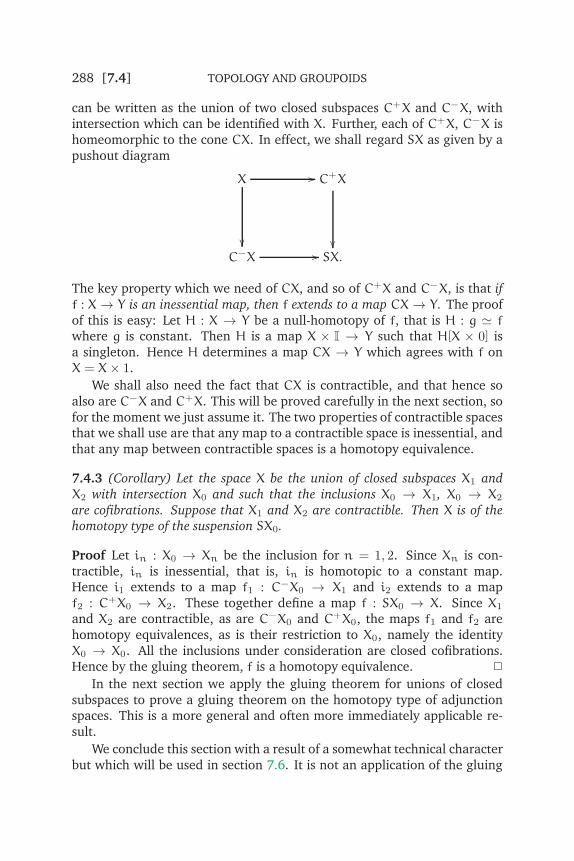
288 [7.4] TOPOLOGY AND GROUPOIDS
can be written as the union of two closed subspaces C+X and C−X, withintersection which can be identified with X. Further, each of C+X, C−X ishomeomorphic to the cone CX. In effect, we shall regard SX as given by apushout diagram
X //
��
C+X
��C−X // SX.
The key property which we need of CX, and so of C+X and C−X, is that if
f : X→ Y is an inessential map, then f extends to a map CX→ Y. The proofof this is easy: Let H : X → Y be a null-homotopy of f, that is H : g ≃ fwhere g is constant. Then H is a map X × I → Y such that H[X × 0] isa singleton. Hence H determines a map CX → Y which agrees with f onX = X× 1.
We shall also need the fact that CX is contractible, and that hence soalso are C−X and C+X. This will be proved carefully in the next section, sofor the moment we just assume it. The two properties of contractible spacesthat we shall use are that any map to a contractible space is inessential, andthat any map between contractible spaces is a homotopy equivalence.
7.4.3 (Corollary) Let the space X be the union of closed subspaces X1 and
X2 with intersection X0 and such that the inclusions X0 → X1, X0 → X2
are cofibrations. Suppose that X1 and X2 are contractible. Then X is of thehomotopy type of the suspension SX0.
Proof Let in : X0 → Xn be the inclusion for n = 1, 2. Since Xn is con-tractible, in is inessential, that is, in is homotopic to a constant map.Hence i1 extends to a map f1 : C−X0 → X1 and i2 extends to a mapf2 : C+X0 → X2. These together define a map f : SX0 → X. Since X1
and X2 are contractible, as are C−X0 and C+X0, the maps f1 and f2 arehomotopy equivalences, as is their restriction to X0, namely the identityX0 → X0. All the inclusions under consideration are closed cofibrations.Hence by the gluing theorem, f is a homotopy equivalence. ✷
In the next section we apply the gluing theorem for unions of closedsubspaces to prove a gluing theorem on the homotopy type of adjunctionspaces. This is a more general and often more immediately applicable re-sult.
We conclude this section with a result of a somewhat technical characterbut which will be used in section 7.6. It is not an application of the gluing

COFIBRATIONS [7.4] 289
theorem, but is placed here because it requires the notion of maps andhomotopies of maps which were defined at the beginning of the section.
Let i : A → X and j : B → Y be two inclusions of subspaces. By a mapof pairs f : (X,A) → (Y,B) is meant a map of maps (f0, f) : i → j, that isa map f : X → Y such that f[A] ⊆ B, and where f0 denotes the restrictionf | A,B. By a homotopy f ≃ g of such maps we mean simply a homotopy ofmaps as defined previously, and this is just a homotopy ft such that f0 = f,f1 = g, and ft[A] ⊆ B for all t. We say f is deformable into B if there is ahomotopy f ≃ g such that g[X] ⊆ B. If also the homotopy is under A thenwe say that f is deformable into B under A.
7.4.4 Let f : (X,A)→ (Y,B) be a map of pairs such that f is deformable into
B. Assume that the inclusion i :A→ X is a cofibration. Then f is deformable
into B under A.
Proof Let j : B → Y denote the inclusion. Let ft be a homotopy (f0, f) ≃(g0,g) such that g[X] ⊆ B. Let α denote the class in πBA of the restrictionof the homotopy ft to a homotopy f0 ≃ g0. Let β = j∗α in πYA. Weconsider the diagram
[(X, i), (B,g0)](−α) || || //
j∗
��
[(X, i), (B, f0)]
j∗
��[(X, i), (Y, jf0)]
β || || // [(X, i), (Y, jg0)](−β) || || // [(X, i), (Y, jf0)].
Let θ in [(X, i), (Y, jf0)] be the class of f : X→ Y so that
β || || (θ) = cls g.
But g[X] ⊆ B and so g = jg ′, where g ′ is the restriction of g to a mapX → B. Let ϕ = cls g ′. Then β || || (θ) = j∗ϕ and so since the above diagramis commutative
θ = (−β) || ||β || || (θ)
= (−β) || || j∗(ϕ)
= j∗(−α) || || (ϕ).
So if h : X → B represents (−α) || || (ϕ) then jh represents θ = cls f. Hence fis homotopic under A to jh. ✷

290 [7.5] TOPOLOGY AND GROUPOIDS
It should be confessed that a simpler proof of this result is possible[Exercise 5], but the above proof is given here as another illustration of theuse of the operations.
EXERCISES
1. Generalise 7.4.3 to the case where X is the union of closed subspaces X1, . . . ,Xn
such that if X0 is the intersection of the Xi then
(i) each inclusion X0 → Xi is a cofibration,
(ii) Xi ∩ Xj = X0 if i 6= j,and similar conditions hold for Y.
2. Let f : (X,A) → (Y,B) be a map of pairs such that B is a deformation retract of
Y. Prove that f is deformable into B under A.
3. Let the inclusion A → X be a cofibration, let B ⊆ Y and let Ft be a homotopy
such that (i) F1[X] ⊆ B, (ii) F0 and F1 agree on A, (iii) F0 mapsA homeomorphically
to B. Prove that F0 is homotopic to F1 relA. [Model the proof of 7.4.4.]
4. Prove 7.2.8 (Corollary 1), 7.2.11 and 7.2.12 using the previous exercise.
5. Let Rt : X× I→ X× I be a retracting homotopy of X× I onto W = X× 1∪A× I,so that R0 = 1, Rt[X× I] ⊆W and Rt is a homotopy rel W. Let Ft : (X,A)→ (Y,B)
be a homotopy deforming F0 into B. Prove that the homotopy (x, t) 7→ FRt(x, 0)
deforms F0 into B rel A.
6. Let f : (X,A) → (Y,B) be a map of cofibred pairs. Prove that f has a right
homotopy inverse if (i) f : X→ Y is a homotopy equivalence and the restriction f0 :
A → B of f has a right homotopy inverse, or (ii) there is a map g : (Y,B) → (X,A)
such that fg ≃ 1Y and f0g0 ≃ 1B.
7. Prove that {0} is not a deformation retract of CL.

COFIBRATIONS [7.5] 291
7.5 The homotopy type of adjunction spaces
Suppose we are given an adjunction space B f⊔ X so that we have a pushout
Af //
i
��
B
i
��X
f// B f⊔ X.
(7.5.1)
In this section we shall apply the gluing theorem from the previous sectionto show that if i is a cofibration then the homotopy type of B f⊔ X dependsonly on the homotopy class of f and on the homotopy types of B and of themap i.
We first need some simple lemmas on deformation retracts.
7.5.2 Let A ⊆ D ⊆ X and let D be a deformation retract of X. Then B f⊔ Dis a deformation retract of B f⊔ X.
Proof Let Rt : X→ X be a retracting homotopy of X onto D. Let
Ft = fRt : X→ B f⊔ X, Gt = i : B→ B f⊔ X.
Then Fti = Gtf (since D contains A); by Remark 7.3.6, Ft and Gt define ahomotopy Ht : B f⊔ X→ B f⊔ X. It is easily checked that Ht is a retractinghomotopy of B f⊔ X onto B f⊔ D. ✷
Intuitively, 7.5.2 is ‘obvious’, since the homotopy which retracts X downontoD also retracts B f⊔ X onto B f⊔ D. But this last statement, although itcontains the essential idea, is not accurate and also does not indicate whythe resulting homotopy is continuous.
7.5.2 (Corollary 1) If A is a deformation retract of X, then B is a deformation
retract of B f⊔ X.
Proof Take A = D in (7.5.1). ✷
We recall that {0} is a deformation retract of I. It follows easily that, forany A, A × 0 is a deformation retract of A × I; so the following result isimmediate.
7.5.2 (Corollary 2) For any A, the vertex of the cone CA is a deformation
retract of CA.
A similar argument shows that if f : A → B is a map then B is a defor-

292 [7.5] TOPOLOGY AND GROUPOIDS
mation retract of the mapping cylinder [Example 2 of Section 7.3]
M(f) = B f′⊔ (A× I)
where f ′ : A × 0 → B is (a, 0) 7→ fa. In fact, if r : A × I → A × 0 is themap (a, t) 7→ (a, 0), then r is a deformation retraction, and therefore soalso is the map q :M(f)→ B which is defined by the maps 1B and f ′r. Letj : A →M(f) be the map a 7→ (a, 1) by which we identify A as a subspaceof M(f). Then we have a commutative diagram,
M(f)
q
��✺✺✺
✺✺✺✺
✺✺✺
A
j
DD✠✠✠✠✠✠✠✠✠✠
f// B
in which j is an inclusion and q is a deformation retraction. This ‘factorisa-tion’ of f is very useful.
7.5.3 The map f : A → B is a homotopy equivalence if and only if A is a
deformation retract of M(f).
Proof We know that q is a homotopy equivalence. Therefore, j is a homo-topy equivalence if and only if f is a homotopy equivalence. But (M(f),A)
is cofibred [Section 7.3]. By 7.2.8 (Corollary 1) j is a homotopy equivalenceif and only if A is a deformation retract of M(f). ✷
This result shows that two spaces are of the same homotopy type if andonly if there is a third space containing each as a deformation retract.
Consider again the adjunction space B f⊔ X of diagram (7.5.1). In orderto study the homotopy type of this space it is convenient to use some auxil-iary space, namely, M(f), M(f)∪X and M(f); these spaces are representedin the following figure.

COFIBRATIONS [7.5] 293
B f⊔ X M(f)
M(f) ∪ XM(f)
q
j ′
B
A
B
X A
X A
BB
X
Fig. 7.8
By 4.6.1 M(f) ∪ X is a subspace of M(f)—we write j ′ for the inclusionmap. Let q : M(f) → B f⊔ X be the standard deformation retraction. Itturns out that if (X,A) is cofibred then qj ′ is a homotopy equivalence, andtherefore, in this case, B f⊔ X can be replaced by M(f) ∪ X. The gluingtheorem 7.4.3 may then be conveniently applied to the union M(f) ∪ X.
7.5.4 If (X,A) is cofibred, then
p = qj ′ :M(f) ∪ X→ B f⊔ X
is a homotopy equivalence relB.
Proof We know q is a homotopy equivalence relB. 7.2.8(Corollary 2)yields that X × 1 ∪ A × I is a deformation retract of X × I. By 7.5.2 withA,D,X replaced by A× 1, X× 1∪A× I, X× I respectively (and with X× 1
identified with X), M(f) ∪ X is a deformation retract of M(f). Thus j ′ alsois a homotopy equivalence relB. ✷
As a simple example of the previous result, let X = S2, let A consist ofthe North and South Poles of S2, and let B consist of a single point. Then theadjunction space B f⊔ X is simply S2 with North and South Poles identified.On the other hand, M(f) ∪ X is homeomorphic to S2 with an arc C joiningthe North to the South Pole. 7.5.4 shows that the map M(f) ∪ X→ B f⊔ Xwhich shrinks C to a point is a homotopy equivalence.

294 [7.5] TOPOLOGY AND GROUPOIDS
B f⊔ X M(f) ∪ XFig. 7.9
The preceding result is false without some assumptions on the pair(X,A) [cf. the Example on p. 298].
We now show that the homotopy type of M(f) ∪ X depends only on thehomotopy class of f.
Suppose that ft : f0 ≃ f1 is a homotopy of maps A→ B. Let
F :M(f0) ∪ X→M(f1) ∪ X
be the identity on B and on X, and on the part A × ]0, 1] of the mappingcylinder be given by
F(a, t) =
{f2ta, 0 < t 6 1
2
(a, 2t− 1), 126 t 6 1
(where (a, 1) is identified with a). The map F is illustrated for the caseX = A = {a} in Fig. 7.8 which amalgamates the pictures of M(f0), M(f1).The proof of the continuity of F is left as an exercise.
a
a
f0a f1aB
Fig. 7.10
7.5.5 The above map F is a homotopy equivalence rel(B ∪ X).
Proof Let G = F | M(f0),M(f1), and let iε : B → M(fε) (ε = 0, 1) be theinclusion. Since G is the identity on B, Gi0 = i1. Since i0, i1 are homotopy

COFIBRATIONS [7.5] 295
equivalences, so also is G. Since G | B ∪ A, B ∪ A is the identity, and(M(fε),B∪A) is cofibred, G is actually a homotopy equivalence rel(B∪A)[7.2.8 (Corollary 1)]. Since F is the identity on X, it follows that F is ahomotopy equivalence rel(B ∪ X). ✷
7.5.5 (Corollary 1) If (X,A) is cofibred and f0 ≃ f1 : A → B, then there is a
homotopy equivalence
B f0⊔ X→ B f1⊔ X relB.
Proof This follows from 7.5.5 and 7.5.4. ✷
As a simple application of this fact, note that if B is path-connected thenB f⊔ E1 (where f : S0 → B) is always of the homotopy type of B∨ S1.
We now show the dependence of the homotopy type of B f⊔ X on the ho-motopy types of B and of the map i : A→ X. Suppose given a commutativediagram of maps
Af //
ϕ0
��❄❄❄
❄❄❄❄
❄
i
��
B
ϕ2
❅❅❅
❅❅❅❅
❅
i��
C
j
��
g // D
j
��
Xf
//
ϕ1��❄
❄❄❄❄
❄❄❄ Q
ϕ
��❄❄❄
❄❄❄❄
❄
Yg
// R
(7.5.6)
where i and j are inclusions of closed subspaces.
7.5.7 (Gluing theorem for adjunction spaces) Suppose i and j are closed
cofibrations and the front and back squares of (7.5.6) are pushouts, deter-mining Q and R as adjunction spaces
Q = B f⊔ X, R = D g⊔ Y.
Suppose that ϕ0, ϕ1, and ϕ2 are homotopy equivalences. Then the map
ϕ : B f⊔ X→ D g⊔ Y
determined by ϕ0,ϕ1,ϕ2 is a homotopy equivalence.

296 [7.5] TOPOLOGY AND GROUPOIDS
Proof The main point of the proof is to replace the adjunction spaces Q =
B f⊔ X, R = D g⊔ Y by the corresponding homotopy pushoutsQ ′ =M(f)∪X,R ′ =M(g) ∪ Y. The diagram (7.5.6) determines a map ψ : Q ′ → R ′ whichagrees with ϕ1 on X, with ϕ2 on B, and with ϕ0 × 1 on A× ]0, 1[. There isa commutative diagram
M(f)ψ2
//
q
��
M(g)
q′
��B
ϕ2// D
in which ψ2 is the restriction of ψ and the vertical maps are the standarddeformation retractions. Since ϕ2, q and q′ are homotopy equivalences, itfollows that ψ2 is a homotopy equivalence.
We now apply the gluing theorem 7.4.3 with
X0 = A, X1 =M(f), X2 = X,
Y0 = C, Y1 =M(g), Y2 = Y
to the map ψ. The cofibration and homotopy equivalence conditions for7.4.3 are satisfied. It follows that ψ is a homotopy equivalence.
However the following diagram is commutative:
M(f) ∪ X ψ //
p
��
M(g) ∪ Y
p ′
��B f⊔ X ϕ // D g⊔ Y
where the vertical maps are the homotopy equivalences of 7.5.4. Since alsoψ is a homotopy equivalence, it follows that ϕ is a homotopy equivalence.
✷
7.5.7 (Corollary 1) Let (ϕ0,ϕ1) : i → j be a homotopy equivalence of maps
where i : A → X and j : C → Y are closed cofibrations. Let g : C → D be a
map. Then the induced map
ϕ : D gϕ0⊔ X→ D g⊔ Y

COFIBRATIONS [7.5] 297
determined by (ϕ0,ϕ1) is a homotopy equivalence.
Proof This is the case B = D, ϕ2 = 1 of 7.5.7. ✷
7.5.7 (Corollary 2) Let i : A→ X be a closed cofibration and let f : A→ B be
a homotopy equivalence. Then the induced map
f : X→ B f⊔ X
is a homotopy equivalence.
Proof This is the following special case of 7.5.7:
A1 //
1��❅
❅❅❅❅
❅❅❅
i
��
A
f
❆❆❆
❆❆❆❆
❆
i��
A
i
��
f // B
i
��
X1
//
1 ��❄❄❄
❄❄❄❄
❄ Xf
❅❅❅
❅❅❅❅
❅
Xf
// Q.
Since f and the identity maps A → A and X → X are homotopy equiva-lences, it follows that f is a homotopy equivalence. ✷
7.5.7 (Corollary 3) If i : A → X is a closed cofibration and A is contractible,
then the identification map p : X→ X/A is a homotopy equivalence.
Proof This is the case of the previous corollary when B consists of a singlepoint. ✷
This last corollary has the following simple proof. Let Ft : A → A bea homotopy such that F0 = 1 and F1 is constant. Let i : A → X be theinclusion. Then iFt extends to a homotopy Gt : X → X such that G0 = 1
and G1[A] is a single point of A. Therefore, G1 defines a map g : X/A→ X
such that gp = G1—whence gp ≃ 1X. Also, since Gt[A] ⊆ A, Gt definesa homotopy Ht : X/A → X/A such that H1p = pGt. Here H0 = 1X/A andH1p = pG1 = pgp, whence H1 = pg. This proves that g is a homotopyinverse of p.
Similar proofs can be given for some other cases of 7.5.7 (Corollary 2)(this remark is useful in the solution of Exercise 8).

298 [7.5] TOPOLOGY AND GROUPOIDS
7.5.7 (Corollary 2) is often useful when combined with 4.5.8 as follows.Suppose given a Hausdorff space Q, a closed subspace B of Q and a closedsubspace A of the compact space X. Let h : X → Q be a map such thath[A] ⊆ B and h | X \A,Q \ B is defined and is a bijection. Let f = h | A,B.Finally, let (X,A) be cofibred.
7.5.8 Under these conditions, if f : A → B is a homotopy equivalence, then
so also is h : X→ Q.
Proof By 4.5.8 there is a homeomorphism g : B f⊔ X → Q such thatgf = h. By 7.5.7 (Corollary 2) f is a homotopy equivalence. Therefore h isa homotopy equivalence. ✷
The previous results are false without some conditions on the pair(X,A).
EXAMPLE
1. Consider the subspaces of R
Y = {0} ∪⋃
n>1
[1
2n,
1
2n− 1
], B = {0, 1}∪
⋃
n>1
[1
2n+ 1,1
2n
].
Let i : L→ B be the inclusion, let f = q :M(i)→ B, A =M(i), X = A ∪ Y.Then B f⊔ X ∼= B i⊔ Y ∼= I. But X is not path-connected (draw the pictureand compare with Example 2, p. 80). So f is not a homotopy equivalenceeven though f is.
We now give some applications of the preceding results, first of all usingonly 7.5.5 (Corollary 1).
(i) (ii) (iii)
a
a a a
a
a
a
Fig. 7.11
The dunce’s hat is obtained from a triangle by identifying the sides ac-cording to the pattern shown in the above figure. Two steps in the iden-tification are shown; the final step is the identification of the two thicklydrawn circles in (iii). The following, somewhat intuitive, discussion showsthat the dunce’s hat is contractible.

COFIBRATIONS [7.5] 299
We can think of the dunce’s hat as a adjunction space S1 f⊔ ∆2 wheref : ∆2 → S1 is determined by the identification shown in (i). In fact,regarding each side a of ∆2 as a map of a line segment onto S1, we canwrite
f = a+ a− a.
It is clear that f is homotopic to the obvious homeomorphism g : ∆2 → S1.But S1 g⊔ ∆2 is homeomorphic to E2. By 7.5.5 (Corollary 1), the dunce’shat is of the homotopy type of E2 and so is contractible.
Our next applications are to joins and smash products. For the remain-der of this section all spaces will be assumed pointed, compact, and Hausdorff.
The base points of X, Y are to be x0,y0 respectively. The base point of X ∗ Ywill then be e = 1
2x0 +
12y0; the base point of SX will be the top vertex v1
(i.e., the set X×1). We will also identify X∨Y with the space obtained fromX⊔ Y by identifying the base point of X with that of Y. In CZ we identify Zwith the subspaceZ× 1 by the map z 7→ (z, 1).
7.5.9 There is a homotopy equivalence
S(X× Y)→ (X ∗ Y)∨ SX∨ SY.
Proof
C−
D
C+
ν1
ν0
S(X × Y) Z = X ∗ Y ∪CX ∪ CY
α
X
Y
e
Fig. 7.12
The points of S(X×Y) we write as (z, t) for z in X×Y and t in I, so that(z, 0) = v0, (z, 1) = v1, for any z in X × Y. Let C−, C+, D be respectivelythe set of points (z, t) such that t > 3
4, t 6 1
4, 1
46 t 6 3
4. Obviously, we
have a homeomorphism from S(X× Y) to
W = (X× Y × I) ∪ C(X × Y × 0) ∪ C(X× Y × 1)
in which, C−, C+, D are mapped to C(X×Y×1), C(X×Y×0) and X×Y×Irespectively. So we now replace S(X× Y) by W.
300 [7.5] TOPOLOGY AND GROUPOIDS
Consider the maps
p : C(X× Y × 0)→ CX p ′ : C(X× Y × 1)→ CY
(x,y, 0, t) 7→ (x, t), (x,y, 1, t) 7→ (y, t),q : X× Y × I→ X ∗ Y
(x,y, s) 7→ (1− s)x + sy.
Clearly p,p ′ agree with q on X× Y× I; therefore, these maps define a map
α :W → Z = X ∗ Y ∪ CX ∪ CY.
Now p,p ′ are homotopy equivalences, since they each are maps from acontractible space to a contractible space. By 7.5.8 α is a homotopy equiv-alence (in 7.5.8 take X = W, A = C(X × Y × 0) ∪ C(X × Y × 1); thefact that (X,A) is cofibred is an easy consequence of results of section7.3). We complete the proof by showing that Z is of the homotopy typeof (X ∗ Y)∨ SX∨ SY.
The inclusion t : X → X ∗ Y is homotopic to the constant map c withvalue y0, since a homotopy i ≃ c is given by
(x, t) 7→ (1− t)x + ty0
(in Fig. 7.12, the shaded face of X ∗ Y is homeomorphic to CX, and thishomotopy is simply sliding X up the cone). Also, c itself is homotopicto the constant map with value e (such a homotopy is given by (x, t) 7→(1 − t)y0 + te). Since i is the attaching map of the cone CX and CX/X ishomeomorphic to SX, it follows from 7.5.5 (Corollary 1) that Z is of thehomotopy type of
((X ∗ Y)∨ SX) ∪ CY.A similar argument shows that this space is of the homotopy type of (X ∗Y)∨ SX∨ SY. ✷
A pointed space X is called well-pointed if (X, {x0}) is cofibred. We recallthat all spaces are assumed compact and Hausdorff.
7.5.10 There is an identification map
X ∗ Y → Σ(X ||||
Y)
which is a homotopy equivalence if X and Y are well-pointed.
Proof We proved in chapter 5 that Σ(X ||||
Y) is homeomorphic to an identi-fication space (X ∗ Y)/R. Thus, to complete the proof we have only to showthat if X, Y are well-pointed then R is contractible and (X ∗Y,R) is cofibred.

COFIBRATIONS [7.5] 301
X
y0
L
x0
Y
R
Fig. 7.13
Let L be the subspace of R of points rx0+sy0. Then R is the union of twocones with a common ‘generator’ L. The inclusion L → CX is a homotopyequivalence, since both L and CX are contractible. Also (X × I,X × 0 ∪x0 × I) is cofibred by 7.3.8 and hence so also does (CX,Cx0) = (CX, L).By 7.2.8 (Corollary 1) L is a deformation retract of CX. Similarly, L is adeformation retract of CY and it follows that L is a deformation retract ofR. Therefore, R is contractible, since L is contractible.
Let J : X× Y × ∆1 → X ∗ Y be the identification map of 5.7.2 (Corollary1). Then
J−1[R] = x0 × Y × ∆1 ∪ X× y0 × ∆1 ∪ X× Y × ∆1.
Now 7.3.7 applied to the product of the three pairs (X, x0), (Y,y0) and(∆1,∆1) show that (X×Y×∆1, J−1[R]) is cofibred. Since J is an identificationmap, it follows that (X ∗ Y,R) is cofibred, and the proof is complete. ✷
7.5.11 If X is well-pointed then the identification map
SX→ ΣX = SX/Sx0
is a homotopy equivalence.
Proof By an argument similar to that in 7.5.10 the pair (SX, Sx0) is cofi-bred. Since Sx0 is contractible, the result follows. ✷
7.5.12 If X and Y are well-pointed then there is a homotopy equivalence
Σ(X× Y)→ Σ(X ||||
Y)∨ ΣX∨ ΣY.
Proof As base point of X × Y we take (x0,y0) where x0,y0 are the basepoints of X, Y respectively. By 7.3.2, X× Y is well-pointed and so Σ(X × Y)is of the same homotopy type as S(X× Y). Similarly, we have a map
(X ∗ Y)∨ SX∨ SY → Σ(X ||||
Y)∨ ΣX∨ ΣY

302 [7.5] TOPOLOGY AND GROUPOIDS
which is a homotopy equivalence on each ‘summand’ of the wedge. By twoapplications of the gluing theorem 7.4.3, this map is a homotopy equiva-lence (we leave the reader to verify the necessary cofibration conditions).The result now follows from 7.5.9. ✷
7.5.12 (Corollary 1) There is a homotopy equivalence
Σ(Sm × Sn)→ Sm+n+1 ∨ Sm+1 ∨ Sn+1.
Proof This is the case X = Sm, Y = Sn of 7.5.12. ✷
EXERCISES
1. Let X,Y,Z be spaces and h : X → Z a map. (i) Let f : X → Y be a map; prove
that there is a map g : Y → Z such that gf ≃ h if and only if h extends over M(f).
(ii) Let g : Y → Z; prove that there is a map f : X → Y such that gf ≃ h if and
only if jh : X → M(g) is deformable into Y (where j : Z → M(g) is the inclusion).
Interpret these statements in the case X = Z, h = 1.
2. Let L have base point 0, and let CL have the same base point as L. Prove that
CL ∨ CL is not contractible. [Let Z = CL ∨ CL and let v1, v−1 be the vertices of
the two cones of Z. Let Ft be a homotopy Z → Z such that F0 = 1, F1 is constant.
Without loss of generality it may be assumed that Ft0 takes the values v1, v−1. Let
αε = inf{t : Ft(0) = vε} for ε = 1,−1. Show that either assumption α1 < α−1,
α−1 < α1 leads to a contradiction.]
3. (i) Let f : L → L× CL be the map x 7→ (x, 0). Prove that f : I → (L × CL) f⊔ Iis not a homotopy equivalence. (ii) Prove that if e ∈ Sn, then Sn/(Sn \ {e}) is
contractible.
4. Prove that if X,Y are compact and Hausdorff then there is a homotopy equiva-
lence
SX× Y/v1 × Y → (X ∗ Y)∨ SX.Deduce that if, further, X, Y are well-pointed, then there is a homotopy equivalence
ΣX× Y/ ·×Y → Σ(X ||||
Y)∨ ΣX.
5. Let X1, . . . ,Xn be compact, Hausdorff, well-pointed spaces. For any non-empty
subset N of {1, . . . ,n} let Zn denote the smash product of the spaces Xi for i in N.
Prove that there is a homotopy equivalence from Σ(X1 × · · · × Xn) to the wedge of
the spaces ΣZN for all non-empty subsets N of {1, . . . ,n}.
6. Let A be a set of m points in Sn (n > 1). Prove that Sn/A has the homotopy
type of the wedge of Sn with (m− 1) circles.
7. Let A be a closed subspace of X. Prove that the following conditions are equiv-
alent: (i) There is a map v : X → I and a homotopy ψt : 1X ≃ ψ1 relA such that
v[A] = {0}, and for all x ∈ X, vx < 1 implies ψ1x ∈ A. (ii) There is a neighbourhood
V of A in X, a map u : X→ I such that u[X \ V] = {1} and u[A] = {0}, and a homo-
topy ϕt : V → X relA such that ϕ0 is the inclusion V → X and ϕ1[V] ⊆ A. [If these
equivalent conditions hold, we say A is a WNDR (weak neighbourhood deformation
retract) of X.]

COFIBRATIONS [7.5] 303
8. Let i : A → X be the inclusion of the closed subspace A of X and let A be
identified as usual with the subspace A × 1 of M(i). Let p : M(i) → X be the
projection. Prove that the following conditions are equivalent: (i) A is a WNDR of
X, (ii) there is a homotopy ht :M(i)→M(i) of the identity relA such that
h1[A× I] ⊆ A, ht[a× I] ⊆ a× I, a ∈ A,
(iii) p :M(i)→ X is a homotopy equivalence relA, (iv) there is a homotopy equiv-
alence M(i)→ X relA, (v) (X,A) has the WHEP. [cf. [Pup67].]
9. Consider the following properties of a pair (X,A), which we label as the rather,
very and completely WHEP. (RWHEP) If f : X → Y is a map and Ut : A → Y is a
homotopy of f | A, then Ut is homotopic rel end maps to a homotopy which extends
to a homotopy of f. (VWHEP) If f : X → Y is a map, u = f | A and u ≃ v, then
some homotopy u ≃ v extends to a homotopy of f. (CWHEP) If u, v : A → Y are
maps and u ≃ v, then u extends over X if and only if v extends over X. Prove that
WHEP ⇒ RWHEP⇒ VWHEP ⇒ CWHEP. Prove also that CWHEP is not a property
invariant under homotopy equivalence of pairs.
10. Show that 7.5.7 (Corollary 3) is true if (X,A) satisfies only the VWHEP.
11. Let f : (X,A) → (Y,B) have homotopy inverse g such that fg ≃ 1 relB. Prove
that if (Y,B) has the VWHEP, then so also does (X,A).
12. Let (X,A), (Y,B) have the WHEP, and let Z = (X × Y)/(X × B ∪ A × Y), with
the usual base point. Prove that (Z, ·) has the WHEP.
13. If f : X → Y is a map, then there is an inclusion map f ′ : Y → C(f) where C(f)
is the mapping cone [Example 5 of Section 4.5]. The following sequence of maps
Xf−→ Y
f′−→ C(f)f′′−→ C(f ′)
f′′′−→ C(f ′′) −→ · · · f(n)
−→ C(f(n−1))
is called the (unpointed, or free) Puppe sequence; here f(n) is defined inductively by
f(n) = (f(n−1)) ′. Prove that there is a diagram, commutative up to homotopy
C(f ′)f ′′′ //
g
��
C(f ′′)
g ′
��SX
Sf// SY
in which g,g ′ are homotopy equivalences.
14. Prove a result similar to that of the previous exercise for the pointed case, in
which C is replaced by Γ and S by Σ.
15. A sequence A1a1←− A2
a2←− A3 ←− · · · of pointed sets and pointed functions is
called exact if for each i > 2, Imai = a−1i−1[·]. A sequence X1
f1−→ X2f2−→ X3 −→ · · ·
of pointed maps of pointed spaces is called exact if the induced sequence of sets
[X1,Z]·f∗1←− [X2,Z]·
f∗2←− [X3,Z]· ←− · · ·

304 [7.6] TOPOLOGY AND GROUPOIDS
is exact for any pointed space—here the base point of [Xn,Z]· is the class of the
constant map and f∗i is clsg 7→ clsgfi. Prove that the (pointed) Puppe sequence is
exact. Deduce that for any pointed map f : X→ Y there is an exact sequence
Xf−→ Y
f′−→ Γ(f) −→ ΣXΣf−→ ΣY
Σf′−→ ΣΓ(f) −→ · · · .
Prove further that if X is a closed subspace of Y, f : X→ Y is the inclusion and (Y,X)
is cofibred, then there is an exact sequence
Xf−→ Y
p−→ Y/X −→ ΣXΣf−→ ΣY −→ Σ(Y/X) −→ · · · .
16. Compare the last sequence with the sequence of sets in the proof of 7.2.12.
17. Let i : X → Y be the inclusion of the closed subspace X of Y. Let (Y,X) be a
pointed pair cofibred. We say X is retractile in Y if Σi : ΣX→ ΣY has a left-homotopy
inverse. Prove that the following conditions are equivalent: (i) X is retractile in Y,
(ii) ΣX is a retract of ΣY, (iii) for each Z the following sequence is exact
0→ [Σ(Y/X),Z]·p∗
−→ [ΣY,Z]·i∗−→ [ΣX,Z]· → 0
where 0 denotes a trivial group [cf. [Jam84]].
18. Prove that if X,Y are well-pointed, then X∨ Y is retractile in X× Y.
19. Let f : X → Y be a pointed map. Prove that Y is retractile in Γ(f) if and only if
Σf is inessential.
20. Let X,Y be well-pointed, compact, and Hausdorff. The homotopy equivalences
X ∗Y → Σ(X ||||
Y), SX→ ΣX, SY → ΣY and the Whitehead product map w : X ∗Y →SX ∨ SY determine a Whitehead product map w ′ : Σ(X |||
|
Y) → ΣX ∨ ΣY uniquely
up to homotopy. Prove that Σw ′ is inessential [cf. [Ark62]].
21. Let X, Y be well-pointed, and let Z = ΣX ∨ ΣY. Let ρ1 : Σ(X × Y) → Z be
i1(Σp1) where p1 : X × Y → X is the projection and i1 : ΣX → Z is the inclusion.
Let ρ2 : Σ(X × Y) → Z be defined similarly as i2(Σp2). Prove that the following
sequence
0→ [Σ(X ||||
Y),Z]·p∗
−→ [Σ(X× Y),Z]· i∗−→ [Z,Z]· → 0
is exact, and that if w ′ is defined as in the previous exercise then
p∗(clsw ′) = −σ2 − σ1 + σ2 + σ1 where σi = cls ρi.
7.6 The cellular approximation theorem
As motivation for the work of this section we consider the following ques-tion: suppose X, B are cell complexes, A is a subcomplex of X and f : A→B is a map; is then B f⊔ X of the homotopy type of a cell complex? Weknow that B f⊔ X is a cell complex if f is a cellular map. Also we knowthat the homotopy type of B f⊔ X depends only on the homotopy classof f (by 7.5.5 (Corollary 1) and since (X,A) is cofibred). Our questionis thus answered by the cellular approximation theorem, a special case of

COFIBRATIONS [7.6] 305
which asserts that any map f : A → B is homotopic to a cellular map. Theword approximation here is used in a rough sense only—we will not beconcerned with questions of metrics nor with a real number ε > 0.
The main technical work is in the following result; the elegant formula-tion of the proof is due to J. F. Adams.
7.6.1 The following statements are true for each n > 1.
α(n) Any map Sr → Sn with r < n is inessential.
β(n) Any map Sr → Sn with r < n extends over Er+1.
γ(n) Let B be path-connected and let Q be formed by attaching a finitenumber of n-cells to B. Then any map
(Er, Sr−1)→ (Q,B)
with r < n is deformable into B.
The proof is by induction by means of the implications
γ(n)⇒ α(n)⇔ β(n)⇒ γ(n+ 1)
the only difficult step being the proof of β(n)⇒ γ(n + 1). The start of theinduction—the proof of γ(1)—is easy; in fact, since E0 consists of a singlepoint and S−1 is the empty set, γ(1) is equivalent to the statement that Qis path-connected, and this is a special case of 4.6.3.
Proof of γ(n)⇒ α(n)
Let f : Sr → Sn be a map such that r < n. Let p : Er → Sr be anidentification map which shrinks the boundary Sr−1 of Er to a point x ofSr, and let e0 = {fx}. Then Sn has a cell structure
Sn = e0 ∪ en
and so fp : Er → Sn defines a map
g : (Er, Sr−1)→ (e0 ∪ en, e0).
The hypothesis γ(n) implies that g is deformable into e0. By 7.4.2 g isdeformable into e0 relSr−1. Throughout this homotopy Sr−1 is mapped tothe point fx, and so, by Remark 7.3.6, this homotopy defines a homotopyf ≃ f ′ : Sr → Sn rel{x} such that f ′ is constant. Thus f is inessential. ✷
Proof of α(n)⇔ β(n)
The proof depends on the fact that there is a homeomorphism Er+1 → CSr
which is the identity on Sr (where Sr is identified with the subset Sr × 1 of

306 [7.6] TOPOLOGY AND GROUPOIDS
CSr). Let p : Sr × I → CSr be the identification map and let g : Sr → Xdenote a constant map.
A homotopy g ≃ f : Sr → X is a map Sr × I → X which is (x, 0) 7→ gx
on Sr × 0 and (x, 1) 7→ fx on Sr × 1. Since g is constant, such a homotopydefines an extension CSr → X of f. Conversely, if f : Sr → X is a map andF : CSr → X is an extension of f, then the composite Fp is a homotopy g ≃ fsuch that g is constant. ✷
Proof of β(n)⇒ γ(n+ 1)
Let Ir denote the boundary of the r-cube Ir, that is, the set of points x of Ir
which have at least one coordinate with a value 0 or 1. The pairs (Er, Sr−1)
and (Ir, Ir) are homeomorphic and so we can assume β(n) in the form thatany map Ir+1 → Sn with r < n extends over Ir+1. Further, since (Ir+1, Ir+1)
is cofibred, we can by (7.2.7) assume that this is true not only for Sn butalso for any space of the homotopy type of Sn.
We assume that
Q = B k1⊔ En+1
k2⊔ En+1 · · · km
⊔ En+1.
Let ki : En+1 → Q be the usual extension of ki : Sn → B. We use thesemaps to define an open cover of Q.
Let Ui be the image under ki of the set {x ∈ En+1 : |x| < 23}, and
let U ′i be the image under ki of the set {x ∈ En+1 : |x| > 1
3}. Let U =
B ∪U ′1 ∪ · · · ∪U ′
m. Then Ui and U are open in Q and we set
U = {U,U1, . . . ,Um}.
Notice that U ∩ Ui is homeomorphic to the space of points x in En+1 suchthat 1
3< |x| < 2
3, and this space is homeomorphic to Sn × ]1
3, 23[. Hence
U ∩Ui is of the homotopy type of Sn, and so we have(*): β(n) can be applied for maps into U ∩Ui rather than Sn.
U ′i Ui U ∩Ui
Fig. 7.14
Suppose now we are given a map
f : (Ir, Ir)→ (Q,B)

COFIBRATIONS [7.6] 307
where r < n+ 1. We must prove that f is deformable into B.By means of hyperplanes in Rr with equations of the the form
xj = s/N, s = 1, . . . ,N− 1, j = 1, . . . , r
we may subdivide Ir into cubes of diameter 6√r/N. By the Lebesgue
covering lemma, N may be chosen so large that each such cube is mappedby f into some set of U.
Let A be the union of all cubes J of all dimensions in this subdivisionsuch that f[J] ⊆ U. Let Kq be the union of all cubes J of dimension 6 q(so that K−1 = ∅, K0 consists of isolated points, and Kr = Ir), and letKq = Kq ∪A.
A
f−1[U]
Fig. 7.15
We construct maps gq : Kq → Q by induction on q so that the followingconditions are fulfilled:1q) gq agrees with f on A, and gq | Kq−1 = gq−1,2q) if x ∈ Kq and fx ∈ Ui then gqx ∈ U ∩Ui.To start the induction we define g−1 to be f | A—clearly conditions 1−1)
and 2−1) are satisfied. Suppose gq has been defined and satisfies 1q) and2q); we extend gq over Kq+1.
Let Jq+1 be a (q + 1)-cube of Kq+1 which is not contained in A. Thenfor some unique i, f[Jq+1] ⊆ Ui and it follows from 2q) that
gq[Jq+1] ⊆ U ∩Ui.
But q + 1 6 r < n + 1, whence q < n. By (*) above, gq extends to a mapJq+1 → U∩Ui, and we define gq+1 : Kq+1 → Q to agree on Jq+1 with thismap. Clearly, conditions 1q+1) and 2q+1) are satisfied, so the induction iscomplete.
Let g = gr : Ir → Q. We prove that f ≃ g.

308 [7.6] TOPOLOGY AND GROUPOIDS
The map ki : En+1 → Q maps the set of points x with |x| < 23
bijectivelyonto Ui: we suppose there is given a linear structure on Ui by means ofthis bijection. We then define a homotopy ht : Ir → Q by
htx =
{fx, fx ∈ no Ui
(1− t)fx+ tgx, fx ∈ some Ui.
Each r-cube Jr in the given subdivision of Ir is mapped by f into U or intosome Ui; thus the formula for ht shows that ht is continuous on Jr. Sincethere cubes from a cover of Ir by closed subsets, this implies the continuityof ht, as a function Ir × I→ Q.
Clearly h0 = f. We prove that h1 = g.Suppose J is an r-cube of the subdivision and x ∈ J. If fx belongs to
some Ui, then the formula for h1 shows that h1x = gx. Suppose fx belongsto no Ui (in which case h1x = fx). Then f[J] is contained in no Ui and sof[J] ⊆ U. Hence x ∈ A and so h1x = fx = gx.
Since Ir ⊆ A the homotopy ht is rel Ir; hence ht defines a homotopyf ≃ g where g : (Ir, Ir)→ (Q,B) is the map defined by g.
Finally, Img ⊆ U and B is a deformation retract of U. Therefore, g isdeformable into B [cf. Exercise 2 of Section 7.4]. ✷
The cellular approximation theorem itself is a consequence of the fol-lowing deformation theorem. (We recall now that the r-skeleton of a cellcomplex K is written Kr.)
7.6.2 Let L be a space and (Lr)r>0 a sequence of subspaces of L such that for
all r > 0
(a) Lr ⊆ Lr+1,
(b) any map (Er+1, Sr)→ (L, Lr) is deformable into Lr+1.
Let K be a cell complex, A a subcomplex of K and f : K→ L a map such that
f[Ar] ⊆ Lr, r = 0, 1, . . . .
Then f is homotopic relA to a map g : K→ L such that
g[Kr] ⊆ Lr, r = 0, 1, . . . .
Proof Let Kr = A ∪ Kr. We construct a sequence of maps fr : K → L andhomotopies fr−1 ≃ fr such that1r), f
r[Ks] ⊆ Ls, 0 6 s 6 r,2r), f
r agrees with fr−1 on Kr−1,3r), f
r−1 ≃ fr relKr−1.The induction is started with f−1 = f when the above conditions are vacu-ously satisfied.

COFIBRATIONS [7.6] 309
By condition (b) any map (Er+1, Sr) → (L, Lr) is deformable intoLr+1 rel Sr. It follows easily, using Remark 7.3.6, that if er+1 is any (r+ 1)-cell of K \ A then fr | Kr ∪ er+1 is deformable into Lr+1 relKr. By ap-plying this to each (r + 1)-cell of K \ A in turn we obtain a homotopyfr | Kr+1 ≃ f ′ relKr such that f[Kr+1] ⊆ Lr+1. Since (K,Kr+1) is cofibredthis homotopy extends to a homotopy fr ≃ fr+1 relKr. Clearly, fr+1 satis-fies 1r+1), 2r+1), 3r+1).
Since K = KN for some N, the map g = fN is the required map. ✷
7.6.2 (Corollary 1) (the cellular approximation theorem). Let K, L be com-
plexes and A a subcomplex of K. If f : K → L is a map such that f | A is
cellular, then f is homotopic relA to a cellular map.
Proof This follows from 7.6.1 γ(n) and 7.6.2 with Lr = Lr. ✷
EXERCISES
1. Let L0 be a subcomplex of L such that for all r > 0 any map (Er+1, Sr)→ (L, L0)
is deformable into L0. Prove that L0 is a deformation retract of L.
2. Let f0, f1 : K → L be cellular maps and A a subcomplex of K. Suppose that
F : f0 ≃ f1 is a homotopy such that for all t ∈ I, Ft[Ar] ⊆ Lr+1, r = 0, 1, . . .. Prove
that F is homotopic relA× I∪K× I to a homotopy G : f0 ≃ f1 such that for all t ∈ I,Gt[K
r] ⊂ Lr+1, r = 0, 1, . . ..
3. Let i : K2 → K be the inclusion of the 2-skeleton of the cell complex K. Prove
that for any subset A of K2, i induces an isomorphism πK2A→ πKA.
4. Prove that Sn is simply connected for n > 1. Prove also that for any point x of
Sn the ith homotopy group πi(Sn,x) [cf. Section 7.1] is 0 for i < n.
5. Prove the cellular approximation theorem for (infinite) CW-complexes.
6. Let K be a connected subcomplex of the complex L. Let j : K→ L be the inclusion
and let x ∈ K0, e ∈ Sr. Prove that any map (Er+1, Sr) → (L,K) is homotopic to a
map h such that he = x.
7. Continuing the notation of the previous exercise, suppose that j∗ : πr(K, x) →πr(L, x) is injective. Let h : (Er+1, Sr) → (L,K) be a map such that he = x. Prove
that h1 : Sr → K is inessential rel e, and hence show that h is homotopic rel e to a
map k such that k[Sr] = {x}.
8. Suppose further to the previous exercise, that j∗ : πr+1(K, x) → πr+1(L, x) is
surjective. Prove that h is deformable into K.
9. Let j : K → L be the inclusion map of the subcomplex K of L. Let K, L be
connected, and suppose j∗ : πr(K, x) → πr(L,x) is an isomorphism for all r > 1
(where x ∈ K0). Prove that K is a deformation retract of L.
10. Let f : K → K ′ be a map of connected complexes such that f∗ : πr(K, x) →πr(K
′, fx) is an isomorphism for all r > 1 (where x ∈ K0). Prove that f is a homo-
topy equivalence.

310 [7.6] TOPOLOGY AND GROUPOIDS
NOTES
The papers [DE72, Sol08], where the second has later citations, giveinteresting results on the condition LEC, which is that for a space X thediagonal ∆ : X→ X × X is a cofibration. For example the first paper showsthat if i : A→ X is a cofibration, then i is injective with closed image whichhas a “halo”.
The notion of cofibration of spaces has a dual version, that of fibration.
For an account of these, see many books on algebraic topology or homotopytheory. The notion of fibration of groupoids [Bro73] was borrowed fromthe notion of fibration of spaces, using the idea that the groupoid I is forgroupoids a kind of model of the unit interval. Fibrations of spaces and ofgroupoids generalise the covering maps of spaces and covering morphismsof groupoids which will be treated in chapter 10. The notion of action of agroupoid on sets generalises the notion of action of a group on a set, whichis important in many branches of mathematics.
The way in which the notion of homotopy occurs in different contextshas lead to a number of abstract homotopy theories (for example [Qui67],[Kam72a], [Mey84], [Bau88]), [KP97]. These have the usual advantagesof abstractions in mathematics, namely of (i) covering several examples atthe same time, (ii) suggesting the possibility of similar methods coveringnew examples, and (iii) simplifying proofs, by allowing the concentrationon essential features. In particular, the gluing theorem for homotopy equiv-alences has been proved in these theories (cf. [Shi84]).
The dual of the gluing theorem is called the cogluing theorem in[BH70]. It is shown in [Hea70] that the gluing theorem follows fromthe cogluing theorem. See [Hea78] for more information on the use ofgroupoid methods in homotopy theory.
The papers [Rut72], [Rut74] give further results on joins and homotopytypes.
The notion of double mapping cylinder is an example of a homotopy
pushout. The general theory of constructions (particularly limits and col-imits) ‘up to homotopy’ is playing an important role in a number of areasof mathematics, such as the applications of algebraic topology to algebraicgeometry (cf. [BK72], [Vog73], [CP86] for some basic results and ideasin this area). For other proofs of the gluing lemma, but with different as-sumptions, see [SW57], [Die71], [Fuc83], [Jam84]. A generalisation of7.2.8 which includes a result both for fibrations and cofibrations is given in[Lam80].
Track groups (i.e. the object groups of πYX) were first studied exten-sively in [Bar55a], [Bar55b], who gave the remarkable calculation that ifX = Y = Sr ∪ er+1, (r > 2), where the cell is attached by a map Sr → Sr of

COFIBRATIONS [7.6] 311
degree 2, then the group of homotopy classes of pointed maps X→ Y, withaddition given by the representation of X as Σ(Sr−1 ∪ er), is cyclic of order4. The easier part of this work, showing that the group concerned was anextension of Z2 by Z2, involved the construction of exact sequences whichwere later generalised to the relative case by [SW57], and also given anelegant formulation by [Pup58] (cf. Exercise 15 of Section 7.5).
The results of section 7.3 have a long history—see the references in[Pup58] and the papers of Strøm ([Str66], [Str69], [Str72]).
I am indebted to conversations with D. Grayson on the notation andstyle of the revision of this chapter.

312 [7.6] TOPOLOGY AND GROUPOIDS

Chapter 8
Some combinatorial
groupoid theory
In this chapter we must build up some of the constructions on groupoidsused in the next chapter to describe various of the groupoids which arise asπXA (for ‘nice’ spaces X) by application of the van Kampen theorem 6.7.2.
Here we encounter the fact that in the first instance groupoids are morecomplicated than groups, so this seems to make for extra difficulties. Onthe other hand, we find that we can use one construction on groupoidsto describe several constructions on groups, such as free groups and freeproducts of groups. The extra ‘spatial component’ to groupoids given by theobjects of a groupoid, allows for constructions on groupoids which modelthe geometry, and make clearer the analogies between between the prop-erties of constructions on spaces and constructions on groupoids.
A key construction on groupoids is to take a groupoid G with object setX and change the object set X by a function σ : X → Y. We will obtaina new groupoid Uσ(G) and a morphism σ : G → Uσ(G) which has a ϕ-universal property, i.e. we can construct morphisms from Uσ(G). Thisconstruction will turn out to imply the constructions of free groupoids andof free products of groupoids, and will also usefully model, as we showin the next chapter, identifications of spaces by changing a discrete wellplaced subspace.
A standard example of such an identification is the changing of the unitinterval [0, 1] by identifying 0 and 1. It is not so clear how to do this mod-elling if you allow only one base point, that is, to consider only groups.
Another construction we need is the analogue of quotient groups by anormal subgroup. This construction is more interesting than in the case
313
314 [8.1] TOPOLOGY AND GROUPOIDS
of groups, and a generalisation of it will be applied in Chapter 11, Section11.3, in connection with orbit spaces under the action of a group. Theunderlying graph structure of a groupoid allows groupoids better to modelthe geometry under consideration than groups alone.
In essence, this chapter sets up some of the basic combinatorialgroupoid theory required for applications.
All these constructions are used in section 9.1 for computing fundamen-tal groups of adjunction spaces, and then for more geometric applications.
8.1 Universal morphisms
We have seen that groupoids model well the product and sum of topolog-ical spaces. In this section, we construct what in full could be called ϕ-universal groupoids with respect to Ob, but which we shall find convenientto call simply universal groupoids and universal morphisms. The universalproperties developed here are a special case of a more general theory in-volving what are called opfibrations of categories, which are important inmany areas of mathematics, and which, as discussed in the Notes at theend of the chapter, tend to have a different terminology from that we usehere.
Certainly the analogy should be borne in mind with the situation for fi-nal topologies, where the forgetful functor giving the underlying set Top→Sets is an opfibration. However, in an algebraic category such as that ofgroupoids the construction of the universal objects is radically differentfrom that for spaces.
Let G be a groupoid, X a set and
σ : Ob(G)→ X
a function. We shall construct from G and σ a groupoid U and morphismσ : G→ U such that (i) Ob(U) = X and (ii) σ is exactly σ on objects.
Our exposition gives the construction first and the universal propertyafterwards, although there is a case for taking the opposite order!
The idea of this construction is as follows (we use multiplicative nota-tion for groupoids throughout most of this chapter). Let a1 ∈ G(x1,y1),a2 ∈ G(x2,y2). Then a2a1 is defined if and only if y1 = x2; in such a case,a morphism σ : G→ U will satisfy
σa2σa1 = σ(a2a1).
Suppose, however, that y1 6= x2 but σy1 = σx2. Then σa2σa1 will bedefined in U but will not necessarily be σb for any b. So, in order to

SOME COMBINATORIAL GROUPOID THEORY [8.1] 315
constructU fromG and σ, we must have a method of constructing elementssuch as σa2σa1. This is done by means of ‘words’ in the elements of G.
Let x, x ′ ∈ X. A word of length n (n > 1) from x to x ′ is a sequence
a = (an, . . . ,a1)
of elements of G such that, if ai ∈ G(xi, x ′i), i = 1, . . . ,n, then(a) x ′i 6= xi+1, i = 1, . . . ,n − 1,(b) σx ′i = σxi+1, i = 1, . . . ,n − 1,(c) σx1 = x, σx ′n = x ′,(d) no ai is the identity.These conditions ensure that no product ai+1ai is defined in G, but thatσai+1σai will be defined in U.
x1
a1
y1
σ σ
x2
a2
y2
Fig. 8.1
The set of all words from x to x ′ of length > 1 is writtenU(x, x ′); exceptthat, if x = x ′, we also include in U(x, x) the empty word of length 0 whichwe write ( )x (and thus suppose that ( )x 6= ( )y when x 6= y).
We now define by induction on length a multiplication
U(x ′, x ′′)×U(x, x ′)→ U(x, x ′′).
The empty word in U(x, x) is to act as identity; that is, if a ∈ U(x, x ′) then
( )x′a = a,a( )x = a.
Suppose that a is as above and b = (bm, . . . ,b1) ∈ U(x ′, x ′′), where bj ∈G(yj,y
′j). We define ba to be, in the various cases:
(bm, . . . ,b1,an, . . . ,a1) if y1 6= x ′n,
(bm, . . . ,b2,b1an,an−1, . . . ,a1) if y1 = x ′n but b1an 6= 1,
(bm, . . . ,b2)(an−1, . . . ,a1) by induction if y1 = x ′n and b1an = 1.

316 [8.1] TOPOLOGY AND GROUPOIDS
This can be expressed as: multiply the two words by putting them end toend, computing in G and cancelling identities where possible.
The definition of multiplication shows that
(an, . . . ,a1)(a−11 , . . . ,a−1
n ) = ( )x′ ,
(a−11 , . . . ,a−1
n )(an, . . . ,a1) = ( )x.
Thus each word has a left and right inverse.We now show that multiplication is associative.
xn
anx ′n z1
c1z ′1
xn−1
an−1x ′n−1 y1
b1y ′1 z2
c2z ′2
Fig. 8.2
Let c = (cr, . . . , c1) ∈ U(x ′′, x ′′′) where ck ∈ G(zk, z ′k). If b is of length0 then certainly c(ba) = ca = (cb)a; this is true, similarly, if a or c is oflength 0. Suppose that m = 1; we check the value of c(ba) and (cb)a ineach case that can arise. These values are
(cr, . . . , c1,b1,an, . . . ,a1) if x ′n 6= y1, y′1 6= z1,
(cr, . . . , c1,b1an,an−1 . . . ,a1) if y′1 6= z1, x ′n = y1, b1an 6= 1,
(cr, . . . , c1b1,an, . . . ,a1) if y′1 = z1, c1b1 6= 1, x ′n 6= y1,
(cr, . . . , c1)(an−1, . . . ,a1) if y′1 6= z1, b1an = 1,
(cr, . . . , c2)(an, . . . ,a1) if x ′n 6= y1, c1b1 = 1,
(cr, . . . , c1b1an,an−1, . . . ,a1) if y′1 = z1, x ′n = y1, c1b1an 6= 1,
(cr, . . . , c2)(an−1, . . . ,a1) if y′1 = z1, x ′n = y1, c1b1an = 1.
If m > 1 we proceed by induction. Write b = b ′′b ′ with b ′,b ′′ shorterthan b. Then
c(ba) = c((b ′′b ′)a) = c(b ′′(b ′a)) = (cb ′′)(b ′a)
= ((cb ′′b ′)a = (cb)a
as was to be shown.So if we take X as the set of objects of U we have proved that U is a
groupoid.

SOME COMBINATORIAL GROUPOID THEORY [8.1] 317
Notice that if x or x ′, does not belong to Imσ, then U(x, x ′) is eitherempty (if x 6= x ′), or contains the identity alone (if x = x ′). Thus U =
U ′ ⊔ U ′′ where U ′ is the full subgroupoid on Imσ and U ′′ is the discretegroupoid on X \ Imσ.
The groupoid U depends on G and on σ, and we therefore write Uσ(G)
for U.
We define a morphism σ : G → Uσ(G) to be σ on objects and to bedefined for a in G(x1, x
′1) by
σa =
{(a), a 6= 1
( )σx1, x1 = x ′1 and a = 1.
Thus σ is injective on the set of non-identities of G and also maps no non-identity to an identity. It is immediate from the definition of the multipli-cation of Uσ(G) that σ is a morphism.
Although the above construction of Uσ(G) gives a good idea of its struc-ture, the important property of Uσ(G) from a general point of view is thatσ satisfies a ϕ-universal property.
Let us, temporarily, identify the set of objects Ob(G) of a groupoid Gwith the wide subgroupoid of G whose elements are all identities: thus weregard Ob(G) as a subgroupoid ofG. (A reader who dislikes this conventionmay instead call this wide subgroupoid Id(G), and replace suitably Ob byId in what follows.)
A morphism f : G→ H of groupoids is said to be universal, or simply tobe a universal morphism if the following square:
Ob(G)Ob(f)
//
i
��
Ob(H)
j
��G
f// H
in which the vertical morphisms are inclusions, is a pushout (in the categoryof groupoids). A useful restatement of this definition is:
8.1.1 A morphism f : G→ H of groupoids is universal with respect to Ob(f)
if and only if for any morphism g : G → K of groupoids and any function
τ : Ob(H)→ Ob(K) such that
Ob(g) = τOb(f)

318 [8.1] TOPOLOGY AND GROUPOIDS
there is a unique morphism g∗ : H → K such that Ob(g∗) = τ and g∗f = g,as shown in the diagram:
Gf
//
g
**Hg∗
//❴❴❴❴❴❴ K
Ob(G)Ob(f)
// Ob(H)τ
// Ob(K)
Proof Let k be the inclusion Ob(K)→ K. Clearly the function τ : Ob(H)→Ob(K) and the morphism τ ′ : Ob(H)→ K determine each other by the ruleτ ′ = kτ. The condition Ob(g) = τOb(f) is equivalent to gi = τ ′ Ob(f), andthe condition Ob(g∗) = τ is equivalent to g∗j = τ ′. So the result followsfrom the definition of pushouts. ✷
From now on we will often abbreviate ‘universal with respect to Ob(f)’simply to ‘universal’.
The pushout property ensures that if f : G → H is universal, then H isdetermined up to isomorphism by Ob(f) and G. On the other hand, givenG and σ : Ob(G) → X, there is a universal morphism f : G → H withOb(f) = σ. This is a consequence of:
8.1.2 Let G be a groupoid and σ : Ob(G) → X a function. The morphism
σ : G→ Uσ(G) is universal.
Proof We use 8.1.1. Let g : G → K be a morphism and τ : X → Ob(K) afunction such that Ob(g) = τσ. Let U = Uσ(G).
We wish a morphism g∗ : U → K such that Ob(g∗) = τ. Thus g isdetermined on the identities of U by τ. An element of U which is not anidentity is a word
a = (an, . . . ,a1), ai ∈ G(xi, x ′i)
such that σx ′i = σxi+1, i = 1, . . . ,n − 1. If n = 1, then we set
g∗(a1) = ga1;
this is the only definition consistent with g∗σ = g. If n > 1, then
gx ′i = τσx′i = τσxi+1 = gxi+1;
therefore we can set
g∗a = gan . . .ga1
= g∗(an) . . .g∗(a1)

SOME COMBINATORIAL GROUPOID THEORY [8.1] 319
the product on the right being defined in K. Clearly, this is the only possibledefinition of a morphism g∗ consistent with g∗σ = g, Ob(g∗) = τ. Tocomplete this proof we verify that this g∗ is a morphism.
Suppose a is as above, b is a word (bm, . . . ,b1) where bj ∈ G(yj,y′j)
and ba is defined. The equation g∗(ba) = g∗bg∗a is clearly true if m or nis 0. Suppose it is true for m = p − 1, n = q − 1. Then for m = p, n = q,referring to the definition of ba, we find that g∗(ba) is
gbm . . .gb1gan . . .ga1 if y1 6= x ′n,
gbm . . .gb2g(b1an)gan−1 . . .ga1 if y1 = x ′n, b1an 6= 1,
g∗((bm, . . . ,b2)(an−1, . . . ,a1)) if y1 = x ′n, b1an = 1.
This is the same as g∗bg∗a by the inductive hypothesis and the fact that gis a morphism. ✷
From now on, we identify each non-identity a1 of G with its image (a1)in Uσ(G).
Let f : G → H be a morphism. We say f is strictly universal if for anymorphism g : G → K such that Ob(g) factors through Ob(f), there is aunique morphism g∗ : H → K such that g∗f = g (this is the same as thecondition in 8.1.1 except that we drop the requirement that Ob(g∗) = τ).
8.1.3 A morphism f : G → H is strictly universal if and only if f is universal
and Ob(f) is surjective.
Proof Suppose f : G → H is a 0-identification. Let σ = Ob(f). The givenuniversal properties imply that there is an isomorphism f∗ : H → Uσ(G)such that f∗f = σ, Ob(f∗) = 1 the identity on Ob(H). It follows easilythat σ : G → Uσ(G) is a 0-identification. This implies that σ = Ob(f) issurjective, for otherwise the condition g∗σ = g does not always determineg∗ on the identities of Uσ(G) which are not images by σ of identities of G.
Suppose given g : G → K and τ : Ob(H) → Ob(K) such that Ob(g) =
τOb(f). Since f is a 0-identification there is a unique morphism g∗ : H→ Ksuch that g∗f = g and Ob(g∗) = τ. But the last condition is redundant,since g∗f = g implies Ob(g∗)Ob(f) = Ob(g) = τOb(f) and so, since Ob(f)is surjective, that Ob(g∗) = τ. ✷
This shows that a strictly universal morphism is analogous to an identi-fication map of topological spaces.
EXAMPLES
1. Let G be a groupoid and σ the unique function from Ob(G) to a singlepoint set {x}. ThenUσ(G) is a groupoid with only one object, that is, Uσ(G)

320 [8.1] TOPOLOGY AND GROUPOIDS
is a group. This group is called the universal group of G and is written UG.The morphism σ : G → UG is universal for morphisms from G to groups,i.e., if g : G → K is a morphism to a group K, then there is a uniquemorphism g∗ : UG→ K such that g∗σ = g. By the construction of UG, theelements of this group are the identity and also all words (an, . . . ,a1) suchthat ai ∈ G, no ai is the identity and no ai+1ai is defined in G.2. In particular, consider the groupoid I with two objects 0, 1 and two non-identities ı, ı−1 from 0 to 1, and 1 to 0 respectively. A word of length n inUI is
ı ı . . . ı or ı−1ı−1 . . . ı−1
and these we can write ın and ı−n respectively. Clearly, there is an isomor-phism UI→ Z which sends ı±n 7→ n.
Notice that the computation of π(S1, 1) in 6.7.5 is now easy—it is im-mediate from 6.7.4 that there is a strictly universal morphism I→ π(S1, 1).3. LetA be a set. A free group onA is a group FA and a function λ : A→ FA
which is universal for functions from A into groups, that is, if µ : A→ G isany function to a group G then there is a unique morphism µ∗ : FA → G
such that µ∗λ = µ. We prove that a free group on A always exists.
Proof Let A be regarded as a discrete groupoid, let FA be the universalgroup of A× I. In the following diagram
Ai //
µ
!!❈❈❈
❈❈❈❈
❈❈❈❈
❈❈❈ A× I
µ′
��✤✤✤✤✤
σ // FA
µ∗
||③③③③③③③
G
i is the function a 7→ (a, ı), σ is the universal morphism and µ is a givenfunction to a group G. The elements µa of G define uniquely a morphismµ′ : A × I → G which sends (a, ı) 7→ µa (so that µ′i = µ). Since µ′ is amorphism to a group, µ′ defines uniquely µ∗ : FA→ G such that µ∗σ = µ′.Hence µ∗σi = µ′i = µ.
Suppose µ : FA→ G is any morphism such that µσi = µ. Then µσ = µ′
whence µ = µ∗. This shows that FA with σi : A→ FA is a free group on A.(We generalise this later to the existence of free groupoids on a graph.) ✷
In the above proof, note that each (a, ı) is a non-identity of A × I; so σis injective on Im i, whence λ = σi is injective. Let us identify each a in Awith λa, so that (λa)−1 is written a−1 (note that a−1 = σ(a, ı−1)). Thenthe non-identity elements of FA are uniquely written as products
aεnn . . .aε1
1 , ai ∈ A, εi = ±1

SOME COMBINATORIAL GROUPOID THEORY [8.1] 321
such that for no i is it true that both ai = ai+1 and εi+1 = −εi.4. Let G,H be groupoids, and let
Gj1−→ K
j2←− H
be morphisms. We say these morphisms present K as the free product ofG and H if the following property is satisfied: if g : G → L, h : H → Lare any morphisms which agree on Ob(G) ∩Ob(H), then there is a uniquemorphism k : K → L such that kj1 = g, kj2 = h. We prove that such a free
product always exists.
Proof Let X = Ob(G) ∪Ob(H) and let
σ : Ob(G) ⊔Ob(H)→ X
be the function defined by the two inclusions into X. Note that σ is alwaysa surjection, and σ is a bijection if and only if Ob(G), Ob(H) are disjoint.
In the following diagram
Gi1 //
j1""❉
❉❉❉❉
❉❉❉❉
❉❉❉❉
❉ G ⊔H
σ
��
Hi2oo
j2||③③③③③③③③③③③③③③
K
i1, i2 are the injections of the coproduct, K = Uσ(G ⊔ H) and j1 = σi1,j2 = σi2. The universal property for j1, j2 is trivial to verify. ✷
Notice that the universal property of the free product can also be ex-pressed by saying that the following square is a pushout
Ob(G) ∩Ob(H)i2 //
i1
��
H
j2
��G
j1// K
where i1, i2 are the inclusions.
The free product of G and H is usually written G ∗H. In particular, letG, H be groups (supposed to have the same object). Then it is clear thatthe injections into the free product G ∗H form a coproduct of groups. If G, H

322 [8.1] TOPOLOGY AND GROUPOIDS
have no common elements, then the elements of G ∗H are the identity andall products
kn . . . k2k1
where (i) each ki belongs to one or other of G, H, (ii) no ki is an identity,(iii) for no i do ki, ki+1 belong to the same group. (When we write G ∗ Hfor groups G, H we will always assume that this is the coproduct of groupsin the above sense.)
The aim of the rest of this section is to determine the universal group ofany connected groupoid. This is useful for the topological applications inChapter 9.
8.1.4 The composite of universal morphisms is universal.
Proof This is immediate from the definition and the fact that a compositeof pushouts is a pushout 6.6.5. ✷
8.1.4 (Corollary 1) Let G be a groupoid and σ : Ob(G) → X, τ : X → Y
functions. Then UτUσ(G) is isomorphic to Uτσ(G).
Proof This is clear from previous results. ✷
8.1.4 (Corollary 2) Let G,H be groupoids. Then the groups
U(G ⊔H), U(G ∗H), UG ∗UHare all isomorphic.
Proof Let X be a set with one object. Consider the commutative diagram
{x,y}
%%▲▲▲▲
▲▲▲▲
▲▲▲▲
▲▲▲▲
▲▲Ob(G) ⊔Ob(H)
σoo
��
τ // Ob(G) ∪Ob(H)
ww♥♥♥♥♥♥♥♥♥♥♥♥♥♥
♥♥♥♥♥♥♥
X
in which the downward functions are constant, τ is the inclusion on Ob(G)
and on Ob(H), and σ maps Ob(G) to x and Ob(H) to y (where x 6= y).Then we obtain a diagram of universal morphisms.
UG ⊔UH
��
G ⊔Hoo //
��
G ∗H
��UG ∗UH U(G ⊔H) U(G ∗H)

SOME COMBINATORIAL GROUPOID THEORY [8.1] 323
By 8.1.4 (Corollary 1), all of the bottom groups in this diagram are isomor-phic. ✷
We now show how to determine UG for any connected groupoid G.First we prove:
8.1.5 Let G be a connected groupoid and T a wide, tree subgroupoid of G.
Then for any object x0 of G, the canonical morphism
G(x0) ∗ T → G
determined by the inclusions, is an isomorphism.
Proof Let ji : G(x0) → G, j2 : T → G be the two inclusions. Each elementa of G(x,y) can be written uniquely as
τya′τ−1
x
for a ′ ∈ G(x0) and τy, τx ∈ T . Therefore, morphisms f1 : G(x0) → K,f2 : T → K which agree on x0 define a morphism f : G→ K by
fa = f2(τy)f1(a′)f2(τ
−1x )
and f is the only morphism such that fj1 = f1, fj2 = f2. ✷
The proof of 8.1.5 shows that the isomorphism G → G(x0) ∗ T is givenby a 7→ τya
′τ−1x (a ∈ G(x,y)).
8.1.6 If T is a tree groupoid, then UT is a free group. If further T has n
objects, then UT is a free group on (n − 1) elements.
Proof Let x0 be an object of T and for each object x of T let τx be theunique element of T(x0, x). Let A be the set of these τx for all x 6= x0, andin the groupoid A × I let ıx, ı
−1x denote respectively (τx, ı) and its inverse
(τx, ı−1).
Let f : A × I → T be the morphism which sends ıx 7→ τx, so thatσ = Ob(f) simply identifies all (τx, 0) to x0. In Uσ(A × I) the only non-identity words are ıx, ı
−1x , ıyı
−1x (x 6= y). So the morphism ϕ : Uσ(A× I)→
T which sends ıx 7→ τx, ı−1x → τ−1
x , ıyı−1x 7→ τyτ
−1x is an isomorphism
such that ϕσ = f. Therefore f is strictly universal. Hence the composite
A × If→ T → UT is strictly universal and so UT is isomorphic to FA, the
free group on A. Finally, if T has n objects, then A has (n − 1) elements.✷
8.1.6 (Corollary 1) If G is a connected groupoid and x0 is an object of G, then
UG is isomorphic to G(x0) ∗ F where F is a free group.
Proof By 8.1.4 (Corollary 2), 8.1.5 and 8.1.6 it is enough to find a widetree subgroupoid T of G. This can be done by choosing for each object

324 [8.1] TOPOLOGY AND GROUPOIDS
x 6= x0 of G an element τx of G(x0, x) and defining T to have all elementsτx, their inverses and their products. The only element of T(x,y) is thenτyτ
−1x and so T is a wide, tree subgroupoid of G. ✷
EXERCISES
1. Define the coproduct ⊔α∈AGα for an arbitrary family in (i) the category of
groupoids, (ii) the category of groups. Prove that if (Gα)α∈A is a family of groupoids,
then the universal group of their coproduct is isomorphic to the coproduct (i.e., free
product) of their universal groups. Hence show that, if G is a groupoid, then UG is
isomorphic to the free product of the groups UGα for all components Gα of G.
2. Let C be a category, let X be a set and σ : Ob(C) → X a surjection. Prove that
there is a category U and a functor σ : C→ U such that (i) Ob(U) = X, Ob(σ) = σ,
(ii) if τ : C → D is any functor such that Ob(τ) factors through σ, then there is a
unique functor τ : U→ D such that τ∗σ = τ.
3. Let f : G → H be a morphism of groupoids such that Ob(G) = Ob(H) = X and
Ob(f) = 1X. Let σ : X → Y be a surjection. Prove that there is a unique morphism
f ′ : Uσ(G) → Uσ(H) such that f ′σ = σf, and that f ′ is injective (on elements) if f
is.
4. Prove that if f : G → H is a strictly universal morphism then f is epic in the
category of groupoids.
5. Prove that if f : G → H, g : H → K are morphisms of groupoids such that gf is
strictly universal and f is epic, then g is strictly universal.
6. A groupoid G is called the internal free product of subgroupoids Gλ if (i) each
identity of G lies in some Gλ, (ii) for each non-identity element x of G there is
a unique sequence λ1, . . . , λn (n > 1) with λi 6= λi+1, and unique non-identity
elements xi in Gλisuch that x = xnxn−1 . . . x1. Prove that G is the internal free
product of the Gλ if and only if the canonical morphism ⊔λGλ → G is strictly
universal. Prove that in such a case, any two distinctGλ meet in a discrete groupoid.
7. Let (Gλ) be a family of subgroups of the groupoid G such that any element x of
G is a product of elements of various Gλ. Prove that G is the internal free product
of the Gλ if and only if the following condition is satisfied: if xi ∈ Gλi(i = 1, . . . ,n;
n > 1) with λi 6= λi+1 (i = 1, . . . ,n − 1) and if xn . . . x1 is defined in G and is an
identity element, then at least one of the xi is an identity element.
8. Suppose there is given a square of groupoid morphisms which is a pushout in
the category of groupoids.
G0
i1 //
i2
��
G1
u1
��G2 u2
// G
Suppose also that σ1 = Ob(u1) and σ2 = Ob(u2) are surjective. Prove that the

SOME COMBINATORIAL GROUPOID THEORY [8.2] 325
following square in which j1 = σ∗1i1, j2 = σ∗2i2, v1 = u∗1, v2 = u∗
2, is also a pushout.
G0
j1 //
j2
��
Uσ1(G1)
v1
��Uσ2
(G2) v2// G
9. Suppose that the first square of the previous exercise is a pushout, that G0,G1
are discrete and that Ob(i2) is surjective. Prove that u2 : G2 → G is a universal
morphism.
10. Let G ′ be a subgroupoid of G and let f : G→ H be a universal morphism. Prove
that there is a subgroupoid H ′ of H such that f restricts to a universal morphism
G ′ → H ′.
11. Compare our exposition of the construction of Uσ(G) with that in [Hig05], and
with the several proofs of normal form theorems for free groups and free products
of groups in [Coh89].
8.2 Free groupoids
The free groupoids generalise the free groups. As the reader will by nowhave expected, free groupoids are defined by means of a universalproperty—to express this we need a little of the language of graph theory.
A graph Γ consists of a set Ob(Γ) of objects (or vertices) and for each x,y in Ob(Γ) a set Γ(x,y) (often called the set of edges from x to y). As usualwe write γ : x → y for γ ∈ Γ(x,y), and x is the initial, y is the final pointof γ. The sets Γ(x,y) for various x, y in Ob(Γ) are supposed disjoint. Inparticular, if x 6= y then Γ(x,y) does not meet Γ(y, x), so that the graphs weare concerned with are often called oriented or directed graphs. As we didfor categories, we shall usually write Γ for the union of the sets Γ(x,y) forany x,y in Ob(Γ), so that a ∈ Γ , or a is an element of Γ , means a ∈ Γ(x,y)for some x,y in Ob(Γ).
An object x of a graph Γ is called discrete (in Γ) if there are no elementsof Γ with initial or final point x. The graph is discrete if all its objects arediscrete.
Let Γ ,∆ be graphs. A graph morphism f : Γ → ∆ assigns to x in Ob(Γ)
and object fx of Ob(∆) and to each a in Γ(x,y) an element fa in ∆(fx, fy).It is easy to verify that the graphs and graph morphisms form a category.
If Ob(Γ) ⊆ Ob(∆), Γ ⊆ ∆ and the inclusion Γ → ∆ is a graph morphism,then we say Γ is a subgraph of ∆: further, Γ is wide in ∆ if Ob(Γ) = Ob(∆);and Γ is full in ∆ if Γ(x,y) = ∆(x,y) for all x,y in Ob(Γ).

326 [8.2] TOPOLOGY AND GROUPOIDS
Suppose Γ ′ is a subgraph of Γ and f : Γ → ∆ is a graph morphism.Then by f[Γ ′] we mean the subgraph ∆ ′ of ∆ whose objects are fx for x inOb(Γ ′), and such that ∆ ′(w, z) is the union of the sets f[Γ ′(x,y)] for all x,yin Ob(Γ ′) such that fx = w, fy = z. In particular, Im f is defined to be thegraph f[Γ ].
The coproduct in the category of graphs is clearly the disjoint union.There is a graph 2 which has two objects 0, 1 and one element ι : 0 → 1.If γ is an element of a graph Γ then there is a unique morphism of graphsγ : 2→ Γ such that γ(ι) = γ.
Given a graph Γ , its dispersion D(Γ) is obtained as a disjoint union ∆ ofcopies of the graph 2, one for each element of Γ , and of a discrete graphon the discrete objects of Γ . The following picture gives an example of thisconstruction:
wc
&&▼▼▼▼
▼▼ y
x
a88qqqqqq
b
&&▼▼▼▼
▼▼
pe
&&▲▲▲▲
▲▲ z
u q
wcc ′
''❖❖❖❖❖
❖ ya
xc xa
a′ 77♦♦♦♦♦♦
pee′
''◆◆◆◆◆
◆ xbb′
''◆◆◆◆◆
◆
u qe zb
Γ D(Γ)
There is a graph morphism ϕ : D(Γ)→ Γ which re-identifies the objects ofD(Γ) to give Γ again: thus D(Γ) has the same discrete objects as Γ but foreach element a : x→ y of Γ there is an element a ′ : xa → ya of D(Γ), andϕ sends xa 7→ x,a ′ 7→ a.
If C is a category then C defines a graph, also written C, simply byforgetting about the composition of elements of C. If f : C→ D is a functor,then f defines also a graph morphism C → D—the converse, of course, isfalse. Since groupoids are special kinds of categories, these remarks applyalso to groupoids and morphisms of groupoids. In particular, we can talkabout subgraphs of a groupoid. Notice that if f : G → H is a morphism ofgroupoids then Im f is a subgraph of H but not usually a subgroupoid. Forexample, if f : I → Z is the strictly universal morphism, then Im f has onlythree elements 0, 1,−1.
Let Γ be as above a graph in a groupoid G. The subgroupoid of Ggenerated by Γ is the intersection of all subgroupoids of G which contain Γ :it is thus the smallest subgroupoid of G containing Γ , and its elements areclearly all identities at points of Ob(Γ) and all products
an . . .a1

SOME COMBINATORIAL GROUPOID THEORY [8.2] 327
which are well defined in G and for which ai ∈ Γ or a−1i ∈ Γ .
We come now to free groupoids. Let Γ be a graph in a groupoid G.We say G is free on Γ if Γ is wide in G and for any groupoid H, any graphmorphism f : Γ → H extends uniquely to a morphism G→ H; and if such Γexists, we say G is a free groupoid.
The free groupoid on the graph 2 is clearly the unit interval groupoid I,and the free groupoid on a discrete graph ∆ is the discrete groupoid on theobjects of ∆. The free groupoid on a coproduct of graphs is the coproductof the free groupoids on each.
8.2.1 Let Γ be a graph in a groupoid G. The following conditions are equiva-lent:
(a) G is free on Γ .
(b) If ϕ : D(Γ) → Γ is the dispersion of Γ , then the induced morphism ϕ :
F(D(Γ))→ G is strictly universal.
(c) Γ generates G and the non identity elements of G can be written uniquely
as products
aεnn . . .aε1
1
such that ai ∈ Γ , εi = ±1 and for no i is it true that both ai = ai+1 and
εi = −εi+1.
Proof We prove (a)⇔ (b)⇔ (c).
(a) ⇒ (b) Let σ = Ob(ϕ). Suppose h : F(D(Γ)) → H is a morphism andτ : Ob(G)→ Ob(H) is a function such that
Ob(h) = τσ.
We first construct from h and τ a graph morphism f : Γ → H.
On objects, f is to be τ; on elements fa = h(a ′). Clearly, f is a graphmorphism. By the assumption that G is free on Γ , f extends uniquely to amorphism h∗ : G→ H. If a ∈ Γ then
h∗ϕ(a ′) = h∗a = fa = h(a ′);
it follows that h∗ϕ = h. Since Γ is wide inGwe must also have Ob(h∗) = τ.
If h : G → H is any morphism such that hϕ = h, then h extends f andso h = h∗. This proves that ϕ is strictly universal.
(b)⇒ (a) Let f : Γ → H be a graph morphism and let τ = Ob(f). We definea morphism h : F(D(Γ)) → H by a ′ 7→ fa. Then Ob(h) = τσ and so thereis a unique morphism h∗ : G → H such that Ob(h∗) = τ and h∗ϕ = h.Thus Ob(h∗) = Ob(f) and for each element a of Γ , h∗a = h(a ′) = fa. Thisshows that h∗ extends f.

328 [8.2] TOPOLOGY AND GROUPOIDS
Let h : G → H be any morphism extending f. Since Γ is wide in G, wehave Ob(h) = Ob(f). Further, if a ∈ Γ , then
hϕ(a ′) = ha = fa
whence hϕ = h. If follows that h = h∗.(b)⇔ (c) This follows from the explicit construction of Uσ(A× I). ✷
8.2.1 (Corollary 1) Let G be a free groupoid on Γ . If f : G → H is strictly
universal, then H is free on f[Γ ]. In particular, UG is a free group.
Proof This follows from 8.2.1 and 8.1.4. ✷
8.2.1 (Corollary 2) Let G be a free groupoid on Γ and let ∆ be a subgraph of
Γ . If H is the subgroupoid of G generated by ∆, then H is free on ∆.
Proof We use 8.2.1(c). First of all, ∆ is certainly wide in H. Next, if a isa non-identity of H, then, since ∆ generates H, a is a product aεn
n . . .aε1
1
such that ai ∈ ∆ and εi = ±1.If for some i we have ai = ai+1, εi = −εi+1, then we can cancel
aεi+1
i+1 aεi
i . Further, we can repeat such cancellations until no relation ofthis form holds. However, since ∆ ⊆ Γ and G is free on Γ , the resultingexpression for a is unique (by 8.2.1(c)). It follows again from 8.2.1(c) thatH is free on ∆. ✷
In fact, any subgroupoid of a free groupoid is free, but this is moredifficult to prove [cf. Section 10.8].
Let G be a free groupoid on Γ . The cardinality of the set of elements ofΓ is called the rank of G. Now it is easy to see from 8.2.1(b) or (c) that noelement of Γ is an identity of G; so, if f : G → H is strictly universal, thenf is injective on the elements of Γ and hence G and H have the same rank.But it may be proved that two free groups are isomorphic if and only if theyhave the same rank [CF63, p. 48]. So the rank of G depends only on G andnot on the particular choice of Γ freely generating G.
IfG,G ′ are two free groupoids on a graph Γ , then the universal propertyshows that there is a unique isomorphismG→ G ′ which is the identity of Γ .On the other hand, given a graph Γ , then 8.2.1(b) shows how to constructa free groupoid FΓ on Γ , while 8.2.1(c) exhibits the elements of FΓ .
Because of the form of elements given in 8.2.1(c), elements of the freegroupoid FΓ on Γ are called paths in Γ , and if w ∈ FΓ(x,y), then w is calleda path from x to y. The graph Γ is called circuit free (or a forest) if all theobject groups of FΓ are trivial, Γ is called a tree if FΓ is a tree groupoid; andΓ is connected if FΓ is connected.
We shall need the following result which is basic in graph theory, butwhose proof is expressed nicely in groupoid language.

SOME COMBINATORIAL GROUPOID THEORY [8.2] 329
8.2.2 If Γ is a connected graph, then Γ contains a tree T which is wide in Γ .
Proof The result is trivial if Ob(Γ) is empty, so we suppose Ob(Γ) non-empty. Let T be the set of all trees contained in Γ ; T is non-empty since itcontains for example a tree with one object and no edges.
Clearly T is partially ordered by inclusion. We claim that an element ofT is maximal in T if and only if it is wide in Γ .
For the proof of the claim, suppose first that T is an element of T whichis wide in Γ . Suppose a is an element of Γ(x,y) such that a does not belongto T .
Let w be the unique element of FT(y, x). Then wa is a non-trivial ele-ment of the group FΓ(x, x), and so T ∪ {a} is not a tree. This contradictionshows that T is maximal.
Suppose, conversely, that T is a tree in Γ which is not wide in Γ . Letx ∈ Ob(T), y ∈ Ob(Γ) \ Ob(T). Since Γ is connected, there is an elementw ∈ FΓ(x,y). Write w = aεn
n . . .aε1
1 as in 8.2.1(c), so that w is a pathtraversing objects x = x1, x2, . . . , xn, xn+1 = y. Let xi be the first of theseobjects which does not lie in T . Let T ′ be obtained from T by adjoiningthe object xi+1 and the edge ai. Then FT ′ is connected. Also FT ′ is a treegroupoid since if u ∈ FT ′(x), then 8.2.1(c) shows that u ∈ FT(x), andhence u = 1, since T is a tree. Since T ′ contains T , it follows that T is notmaximal.
We now show that the set T has a maximal element. If Γ is finite thenthe set T is finite, and so has a maximal element. If Γ is not finite, we mustapply Zorn’s Lemma (cf. Glossary).
Let C be any non-empty ordered subset of T, and let C be the union ofthe elements of C. If x,y ∈ Ob(C), then x,y ∈ Ob(C′) for some C′ in C.Hence FC′(x,y), and so FC(x,y), is non-empty. If u, v ∈ FC(x,y), then by8.2.1(c), u, v ∈ FC′′(x,y) for some C′′ in C containing C′. Hence u = v. SoFC is a tree groupoid, and so C ∈ T.
Hence any non-empty ordered subset of T has an upper bound in T. ByZorn’s Lemma, T has a maximal element T . Then T is wide in Γ . ✷
8.2.3 If G is a connected, free groupoid then each object group G(x) of Gis free. If further G is of rank n1 and has n0 objects, then G(x) is of rank
n1 − n0 + 1.
Proof Let x ∈ Ob(G) and let Γ be a graph freely generating G. It followsfrom 8.2.2 that G contains a tree groupoid T such that T ∩ Γ generates T .For each y in Ob(G) there is a unique element ty of T(x,y). By 6.5.11 (seealso 6.7.3), these elements define retractions r : T → {x}, r ′ : G→ G(x).

330 [8.3] TOPOLOGY AND GROUPOIDS
Let ∆ be the wide subgraph of Γ whose elements are those a in Γ whichdo not lie in T . Let H be the (free) subgroupoid of G generated by ∆. Weclaim that G is the free product T ∗H.
Let us grant this claim for the moment. Consider the diagram
Ob(G) //
��
Tr //
��
{x}
��H
i// G
r ′// G(x)
in which the left-hand square of inclusions is a pushout, since G = T ∗ H,and the right-hand square is a pushout, by 6.7.3. Therefore the compositesquare is a pushout. It follows that r ′i : H→ G(x) is strictly universal, andso G(x) is a free group on r ′[∆].
If G is of rank n1 then Γ has n1 elements. If G has n0 objects thenΓ ∩ T has n + 0 − 1 elements. Then ∆, and so also r ′[∆], has n1 − (n0 − 1)
elements—hence G(x) is of rank n1 − n0 + 1.
To complete the proof we must show that G = T ∗ H. Let t : T → K,h : H → K be morphisms which agree on Ob(G). Let Γ ′ = Γ ∩ T , sothat T is free on Γ ′. Then t,h restrict to graph morphisms t ′ : Γ ′ → K,h ′ : ∆→ K which (since they agree on objects and Γ ′ ∩∆ has no elements)together define a graph morphism f : Γ → K. Since G is free on Γ , f extendsuniquely to a morphism k : G→ K. However k | T extends t ′, k | H extendsh ′. Therefore k | T = t, k | H = h and this proves that t and h extend to amorphism k : G→ H.
If k : G→ H also extends t and h, then k |Γ= f and it follows that k = k.✷
EXERCISES
1. Prove that a groupoid G is free if and only if each component of G is free.
2. Prove that a simply-connected groupoid is free.
3. Prove that the coproduct, and free product of free groupoids is free.
4. Give another proof of 8.2.3 using 8.2.1(b), Exercise 3 of Section 6.7, and Exer-
cise 9 of Section 8.1.
5. Give another proof of 8.2.1 (Corollary 2) using Exercise 10 of Section 8.1.

SOME COMBINATORIAL GROUPOID THEORY [8.3] 331
8.3 Quotient groupoids
Let G be a groupoid. A subgroupoid N of G is called normal if N is wide inG and, for any objects x,y of G and a in G(x,y),
aN(x)a−1 ⊆ N(y)
that is,a××[N(x)] ⊆ N(y).
This last condition implies that (a−1)××[N(y)] ⊆ N(x) and hence, since(a−1)×× = (a××)
−1, we will in fact have
a××[N(x)] = N(y).
EXAMPLE
1. Let f : G → H be a morphism. Then Ker f, the wide subgroupoid ofG whose elements are all k in G such that fk is an identity of H, is anormal subgroupoid of G. In fact, it is obvious that Ker f is wide in G, andnormality follows from
f(aka−1) = fafkfa−1 = fafa−1 = 1, k ∈ N(x), a ∈ G(x,y).
We note also that if Ob(f) is injective then Ker f is totally disconnected.A morphism f : G → H is said to annihilate a subgraph Γ of G if f[Γ ] is
a discrete subgroupoid of H. Thus Ker f is the largest subgroupoid annihi-lated by f.
8.3.1 Let N be a totally disconnected, normal subgroupoid of G. Then there
is a groupoid G/N and a morphism p : G → G/N such that p annihilates Nand is universal for morphisms from G which annihilate N.
Proof We define Ob(G/N) = Ob(G). If x,y ∈ Ob(G) we define G/N(x,y)
to consist of all cosetsaN(x), a ∈ G(x,y).
If a ∈ G(x,y), b ∈ G(y, z) then, by normality,
bN(y)aN(x) = baN(x)N(x)
= baN(x).
Therefore, multiplication of cosets again gives a coset. The associativity ofmultiplication is obvious. The identity element of G/N(x, x) is the coset

332 [8.3] TOPOLOGY AND GROUPOIDS
N(x) and the inverse of aN(x) is a−1N(y) (a ∈ G(x,y)). So G/N is agroupoid.
The morphism p : G→ G/N is the identity on objects, and on elementsis defined by a 7→ aN(x)—clearly p is a morphism and Kerp = N.
The universal property of p is that if f : G → H is any morphism whichannihilates N, then there exists a unique morphism f∗ : G/N → H suchthat f∗p = f. Now the cosets of N are exactly the equivalence classes of theelements of G under the relation a ∼ b ⇔ ab−1 is defined and belongs toN; so a ∼ b ⇔ pa = pb. The universal property follows easily from A.4.6.
✷
Remark 8.3.1 is true on the assumption only thatN is normal [cf. Exercise2]; we need this more complicated construction of G/N in chapter 11, andgive it there. We call G/N a quotient groupoid of G.
The usual homomorphism theorem for groups (that if f : G → H is amorphism then Im f is isomorphic to G/Ker f) is false for groupoids, onereason being that Im f need not be a subgroupoid of H; for example, thestrictly universal morphism f : I→ Z has I/Ker f isomorphic to I. Howeverwe do have:
8.3.2 Let f : G→ H be a morphism such that Ob(f) is injective. Then Im f is
a subgroupoid of H and the canonical morphism
G/Ker f→ Im f
is an isomorphism.
Proof To prove that Im f is a subgroupoid of H, it is sufficient to prove thatif c,d ∈ Im f and d−1c is defined in H, then d−1c ∈ Im f.
Suppose c = fa, d = fb where a ∈ G(x,y), b ∈ G(z,w). Since d−1cis defined, fy = fw, which implies (since Ob(f) is injective) that y = w.Hence, b−1a is defined and d−1c = f(b−1a) which belongs to Im f.
Since f annihilates Ker f, which is a wide, totally disconnected and nor-mal subgroupoid of G, there is a canonical morphism f ′ : G/Ker f → H
such that f ′p = f. Since f ′ is defined by f ′(aKer f) = fa, it is clear thatIm f ′ = Im f. Let f ′′ : G/Ker f→ Im f be the restriction of f ′. Then Ob(f ′′)
is bijective, and for each a,b ∈ G
f ′′(aKer f) = f ′′(bKer f)⇔ fa = fb
⇔ aKer f = bKer f.
It follows from 6.4.3 that f ′′ is an isomorphism. ✷
We now consider relations in a groupoid. Suppose given for each objectx of the groupoid G a set R(x) of elements of G(x)—thus R can be regarded

SOME COMBINATORIAL GROUPOID THEORY [8.3] 333
as a wide, totally disconnected subgraph of G. The normal closure N(R) ofR is the smallest wide normal subgroupoid of G which contains R. This ob-viously exists since the intersection of any family of normal subgroupoidsof G is again a normal subgroupoid of G. Further, N(R) is totally discon-nected since the family of object groups of any normal subgroupoid N of Gis again a normal subgroupoid of G.
Alternatively, N = N(R) can be constructed explicitly. Let x be an objectof G. By a consequence of R at x is meant either the identity of G at x, orany product
ρ = a−1n ρnan . . .a−1
1 ρ1a1 (*)
for which ai ∈ G(x, xi) and ρi, or ρ−1i , is an element of R(xi). Clearly, N(x),
the set of consequences of R at x, is a subgroup of G(x) and the family Nof these groups is a wide totally disconnected subgroupoid of G containingR. Also N is normal, since if a ∈ G(y, x) then
a−1ρa = (ana)−1ρn(ana) . . . (a1a)
−1ρ1a1a
is an element of N(y). On the other hand, any normal, wide subgroupoidof G which contains R must clearly contain all products such as (*) and somust contain N. Hence N = N(R).
The projection p : G → G/N(R) clearly has the universal property :if f : G → H is any morphism which annihilates R then there is a unique
morphism f ′ : G/N(R)→ H such that f ′p = f. We call G/N(R) the groupoidG with the relations ρ = 1, ρ ∈ R.
In applications, we are often given G, R as above and wish to describethe object groups of G/N(R). These are determined by the following result.
8.3.3 Let G be connected, let x ∈ Ob(G) and let r : G→ G(x) be a deforma-
tion retraction. Let H = G/N(R). Then H(x) is isomorphic to the group G(x)
with the relations
r(ρ) = 1, ρ ∈ R.
Proof The deformation retraction r and the morphism p : G → H de-termine as in 6.7.3 a deformation retraction s : H → H(x) such that thefollowing square is a pushout
Gr //
p
��
G(x)
p ′
��H
s// H(x)
(**)

334 [8.4] TOPOLOGY AND GROUPOIDS
where p ′ is the restriction of p. We verify that p ′ satisfies the requireduniversal property.
Let f : G(x) → K be a morphism such that f annihilates r[R], i.e. frannihilates R. Then there is a unique morphism g : H → K such thatgp = fr. Since (**) is a pushout, there is a unique morphism f ′ : H(x)→ Ksuch that f ′p ′ = f, f ′s = g. To complete the proof we must show that thelast condition is redundant as far as the uniqueness of f ′ is concerned.
Let f ′′ : H(x) → K be any morphism such that f ′′p ′ = f. Then f ′′sp =
f ′′p ′r = fr = gp. But p is surjective, so that f ′′s = g. The pushout propertyof (**) now implies that f ′′ = f ′. ✷
EXERCISES
1. Prove that there are morphisms f : I → Z, g : I → Z2 such that Ker f = Kerg
and Im f is not (graph) isomorphic to Img.
2. Let N be any normal subgroupoid of the groupoid G. Prove that there is a
groupoid G/N and morphism p : G → G/N such that p annihilates N and is uni-
versal for this property. [The elements of G/N are equivalence classes of elements
of G under the relation a ∼ b if and only if a = xby for some x,y in N.]
3. Prove that if f : G → H is a morphism with kernel N, then f = pf ′ where
p : G → G/N is the projection and f ′ : G/N → H has discrete kernel. If f ′ is an
isomorphism onto Im f, then we shall call f a projection.
4. Prove that any morphism f can be factored as f = f2f1 where Ob(f1) is the
identity and f2 is faithful [for faithful, cf. Exercise 14 of Section 6.5].
5. Prove that any f : G → H can be factored as f = gr where r is a deformation
retraction and Kerg is totally disconnected.
6. Prove that any deformation retraction is a projection.
7. Prove that if f : G→ H is faithful, then f = gr where r is a deformation retraction
and Ker g is discrete.
8. Prove that any projection is a deformation retraction followed by projection g
with Ob(g) = 1.
9. Prove that the category of groupoids admits coequalisers and deduce that any
morphisms G0 → G1, G0 → G2 have a pushout.
8.4 Some computations
We conclude this chapter with a computation of a pushout of groupoidswhich arises in the determination of the fundamental group of the unionof two connected spaces with non connected intersection, for example asshown in Fig. 8.3.

SOME COMBINATORIAL GROUPOID THEORY [8.4] 335
Fig. 8.3
Note that one of the problems of attempting to solve this question withthe fundamental group alone is that a choice of base point is then required.It is clear that a base point should be in a component of the intersection ofthe two pieces, but it is not clear which component to choose. We thereforeavoid a decision by choosing a set of base points, one in each component ofthe intersection, and so work with groupoids. This strategy of avoidance ofdecision seems to be optimal.
The formulae that we obtain are stated in Van Kampen’s paper on thefundamental group ([Kam33]) but his proof even of the connected case isdifficult to follow.
8.4.1 Suppose given a pushout of groupoids
Ci //
j
��
A
u
��B
v // G
(1)
such that (a) all the groupoids have the same set J of objects, (b) i, j,u, vare the identity on objects, and (c) A and B are connected groupoids, and
C is totally disconnected. Let p be a chosen element of J = Ob(C). Let
r : A → A(p), s : B → B(p) be retractions obtained by choosing elements
αx ∈ A(p, x), βx ∈ B(p, x), for all x ∈ J, with αp = 1, βp ∈ 1. Let
fx = (uαx)−1(vβx) in G(p), and let F be the free group on the elements fx,
x ∈ J, with the relation fp = 1. Then the object group G(p) is isomorphic tothe quotient of the free product group
A(p) ∗ B(p) ∗ F
by the relations
(riγ)fx(sjγ)−1f−1
y = 1 (2)
for all x ∈ J and all γ ∈ C(x).

336 [8.4] TOPOLOGY AND GROUPOIDS
Proof We first remark that the pushout (1) implies that the groupoid Gis isomorphic to the quotient of the free product groupoid A ∗ B by therelations (iγ)(jγ)−1 for all γ ∈ C. The problem is to interpret this fact interms of the object group at p of G.
To this end, let T , S be the tree subgroupoids of A,B respectively gen-erated by the elements αx,βx, x ∈ J. The elements αx,βx, x ∈ J, defineisomorphisms
ϕ : A→ A(p) ∗ T , ψ : B→ B(p) ∗ S
where if g ∈ G(x,y) then
ϕg = αy(rg)α−1x , ψg = βy(sg)β
−1x .
So G is isomorphic to the quotient of the groupoid
H = A(p) ∗ T ∗ B(p) ∗ S
by the relations(ϕiγ)(ψjγ)−1 = 1
for all γ ∈ C. By 8.3.3, the object group G(p) is isomorphic to the quotientof the group H(p) by the relations
(rϕiγ)(rψjγ)−1 = 1
for all γ ∈ C.Now if J′ = J \ {p}, then T , S are free groupoids on the elements αx,βx,
x ∈ J′, respectively. By 8.2.1 (Corollary 1), T ∗ S is the free groupoid on allthe elements αx,βx, x ∈ J′. It follows from 8.2.3, that (T ∗ S)(p) is the freegroup on the elements rβx = α−1
x βx = fx, x ∈ J′. Let fp = 1 ∈ F. Since
rϕiγ = riγ, rψjγ = fy(sjγ)f−1x ,
the result follows. ✷
There is a consequence of the above computation which we shall usein the next chapter in proving the Jordan Curve theorem. First, if F and Hare groups, recall that we say that F is a retract of H if there are morphismsı : F→ H, ρ : H→ F such that ρı = 1. This implies that F is isomorphic to asubgroup of H.
8.4.1 (Corollary) Under the situation of 8.4.1, the free group F is a retract of
G(p). Hence if J = Ob(C) has more than one element, then the group G(p) is
not trivial, and if J has more than two elements, then G(p) is not abelian.
Proof Let M = A(p) ∗ B(p) ∗ F, and let ı ′ : F → M be the inclusion. Letρ′ : M → F be the retraction which is trivial on A(p) and B(p) and is the

SOME COMBINATORIAL GROUPOID THEORY [8.4] 337
identity on F. Let q :M→ G(p) be the quotient morphism. Then it is clearthat ρ′ preserves the relations (2), and so ρ′ defines uniquely a morphismρ : G(p) → F such that ρq = ρ′. Let ı = qi ′. Then ρı = ρ′i ′ = 1. So F is aretract of G(p).
The concluding statements are clear. ✷
Here is another application of the Van Kampen theorem for the funda-mental groupoid, namely to HNN-extensions of groups. This construction isnamed after the initial letters of the authors of the paper which introducedthe construction ([HNN49]).
Our approach also shows the advantage of the use of groupoids: be-cause there is a homotopy theory of groupoids, we can make analogues ingroupoid theory of constructions for spaces, particularly double mappingcylinders.
Let G be a group and let iA : A → G, iB : B → G be inclusions of twosubgroups of G. Suppose given an isomorphism θ : A → B. The aim is toconstruct a new group H = G∗θ which contains A,B as subgroups and inwhich there is an element t ∈ H which conjugates A to B, that is for alla ∈ A we have tat−1 = θa in H.
To this end we form the pushout of groupoids
A× Ii //
j
��
G
ϕ
��A× I
ψ// H.
(8.4.2)
Here j is the inclusion; i is the morphism defined by (a, 0) 7→ iAa, (a, 1) 7→iBθa; and ϕ,ψ are defined by the pushout, so that ϕi = ψj. Hence fora ∈ A, ψ(a, 0) = ϕi(a, 0) = ϕa, ψ(a, 1) = ϕi(a, 1) = ϕθa.
Note that if e denotes the identity element of the group G, and a ∈ A,then, in the multiplication in A × I, we have (a, 1)(e, ı) = (e, ı)(a, 0). Lett = ψ(e, ı) ∈ H. So in H
t(ϕa) = ψ(e, ı)ψ(a, 0)
= ψ((e, ı)(a, 0))
= ψ((a, 1)(e, ı))
= (ψ(a, 1))t
= ϕ(θa)t.
Hence t(ϕa)t−1 = ϕ(θa) in H.

338 [8.4] TOPOLOGY AND GROUPOIDS
Note that this result and construction makes sense whether or not iA :
A → G is injective and whether or not θ is an isomorphism. However itis a standard result of combinatorial group theory, see for example [LS77],that if iA is injective and θ is an isomorphism, then ϕ is also injective. It isin these circumstances that H is called an HNN-extension and written G∗θ.
This is a corollary of a more general result on graphs of groups [Ser80],which has been put in a powerful way in terms of a normal for the elementsof the fundamental groupoid of a graph of groups in [Hig76]. This itselfhas been generalised to the fundamental groupoid of a graph of groupoids inEmma Moore’s Bangor thesis [EJM01] (which is available for download).A consequence of her results is that in the situation of 8.4.1, if i, j areinjective, then so also are u, v.
NOTES
Most of the results on groupoids are due to Higgins ([Hig64], [Hig66],[Hig05]) but the proof of 8.4.1 is new. The proof of the associativity of themultiplication of the words of Uσ(G) is borrowed from the treatment offree products of groups in [Lan65]. The construction of arbitrary colimitsof categories and groupoids is given in [Hig05], and indeed is a special caseof results of [Hig63]. The reader is invited to compare these approaches tothe construction of Uσ(G) with the standard constructions in combinatorialgroup theory of free groups and free products, and the derivation of normalforms. For example [Coh66] discusses four methods for obtaining these.The paper [Hig76] has a very elegant treatment of normal forms for thefundamental groupoid of graph of groups, and a computational form ofthis is in Emma Moore’s thesis [EJM01].
The term ‘combinatorial groupoid theory’ seems appropriate though isnon standard, and it is an area which needs development. It certainlyincludes methods of covering groupoids as presented in Chapter 9, and in[Hig05]. Other contributions are [Bra04, Hum94]. The latter paper, and[EJM01], also deal with computational aspects.
There is an important general theory of fibred, opfibred (or cofibred)and bifibred categories which was initiated by Grothendieck and devel-oped strongly by Jean Benabou. These notions are discussed in for example[Bor94], [Joh02], [Tay99]. In particular, the functor Ob from groupoids tosets is, in these terms, a bifibration (both fibration and opfibration) of cat-egories. Unfortunately, the terminology is not entirely stable (the last citedbooks use the terms ‘prone, supine’ for what was previously called ‘carte-sian, cocartesian’), so we have decided to stick with the terminology ofHiggins which dates back to 1963. However, similar ideas occur in module

SOME COMBINATORIAL GROUPOID THEORY [8.4] 339
theory, with notions of ‘change of ring’, and in the theory of Mackey func-tors, but there again with a different terminology. An account is also givenin [BHS11, Appendix B]. The work of Higgins on universal morphisms ofgroupoids was a stimulus for later work on ‘induced crossed modules’,which are structures which carry homotopical information in dimensions0,1 and 2. The general problem is to develop language and modes of calcu-lation to describe how mathematical structures with information at variouslevels are changed in high levels when changes are made in a low level.

340 [8.4] TOPOLOGY AND GROUPOIDS

Chapter 9
Computation of the
fundamental groupoid
In this chapter we compute the fundamental groupoid of some useful ad-junction spaces, and hence of cell complexes, by applying the methods de-veloped in chapter 8. We then develop some geometric applications, toknots, the Phragmen-Brouwer property, and the Jordan Curve Theorem.
9.1 The Van Kampen theorem for adjunction
spaces
In Section 6.7 we proved a van Kampen theorem for the fundamentalgroupoid πXA when X is given as a union of open subsets.
Suppose given an adjunction space W f⊔ Z as in the pushout square
Yf //
i
��
W
i
��Z
f// W f⊔ Z.
(9.1.1)
Our object is to determine the groupoid
π(W f⊔ Z)B
for certain (useful) B.
341

342 [9.1] TOPOLOGY AND GROUPOIDS
In chapter 7, we studied the homotopy type of W f⊔ Z and showed itsdependence on the homotopy types of W and (Z, Y) if (Z, Y) is cofibred.This is a local condition on Y in Z. To determine the fundamental groupoidπ(W f⊔ Z) as a pushout, we also need some local conditions—these con-ditions are essentially in dimensions 0 and 1, and are described in terms ofthe natural map
p :M(f) ∪ Z→W f⊔ Zand its induced morphism of fundamental groupoids.
Suppose that C is a subset of Z representative in Z and in Y, that D is asubset of W representative in W, and that f[C] ⊆ D. Let
g = f | C ∩ Y,D, B = D g⊔ C.
Under these conditions we have:
9.1.2 (The Van Kampen theorem) The following square
πYCf //
i
��
πWD
i
��πZC
f// π(W f⊔ Z)B
(9.1.3)
is a pushout if and only if the morphism
p : π(M(f) ∪ Z)A→ π(W f⊔ Z)B
in which A = D ∪ C, is a homotopy equivalence of groupoids. In particular,
(9.1.3) is a pushout if (Z, Y) is cofibred.
Proof Let X =M(f) ∪ Z, X2 = X \W, X1 =M(f), X0 = X1 ∩ X2.
W
X X2
W
X1
Fig. 9.1

COMPUTATION OF THE FUNDAMENTAL GROUPOID [9.1] 343
The interiors of X1,X2 cover X and so we are in the position to apply 6.7.4to give us a pushout isomorphic to (9.1.3).
Let A ′ = D, so that in the notation of 6.7.4, A1 = D ∪ (C \ Y). Thenp :M(f) ∪ Z→W f⊔ Z maps A1 bijectively onto B. Further A ′, and hencealso A1, is representative in X1. Indeed, A1 meets each path componentof W because D is representative in W. Also C ∩ Y is representative in Yand each point c of C ∩ Y can be joined by the path down the mappingcylinder of fc, which belongs to D; this path is shown as a thick line in X1
in Fig. 9.1. Notice also that if θc is the class in πX1A of this path, thenp(θc) is the identity at fc in πW.
Consider the following diagram in which (i) Q =W f⊔ Z, (ii) the frontsquare is the pushout determined by A1 and the above elements θc as in6.7.4, (iii) the back square is (9.1.3).
πYC //
∼=""❉
❉❉❉❉
❉❉❉
��
πWD
��
πX0A
i2
��
ri1 // πX1A1
u1
��
∼=p
cc●●●●●●●●●
πZA //
∼= !!❉❉❉
❉❉❉❉
❉ πQB
πX2A su2
// πXA1
pcc❋❋❋❋❋❋❋❋
(9.1.4)
The left-hand square is induced by inclusions and so is commutative.The right-hand square is induced by p and its restrictions, so the right-handsquare is commutative. The commutativity of the top and bottom squaresis a consequence of p(θc) = 1 (c ∈ C ∩ Y). Thus (9.1.4) is commutative.
Each morphism marked ∼= is induced by a homotopy equivalence and isbijective on objects. Therefore these morphisms are isomorphisms. Hence,each of the following statements is equivalent to its successor: (a) (9.1.3)is a pushout, (b) (9.1.4) determines an isomorphism of its front square toits back square, (c) p : πXA1 → πQB is an isomorphism.
However, the last morphism is bijective on objects so (c) is equivalentto (d) p : πXA1 → πQB is a homotopy equivalence. Since πXA1 is adeformation retract of πXA, (d) itself is equivalent to (e) p : πXA → πQBis a homotopy equivalence.
This proves the main part of 9.1.2. The last statement of 9.1.2 follows

344 [9.1] TOPOLOGY AND GROUPOIDS
from 7.5.4. ✷
9.1.2 (Corollary 1) LetW,Z be closed inW∪Z, let (Z,W∩Z) be cofibred and
let B be a set representative in W ∩ Z, W, Z. Then the square of morphisms
induced by inclusions
π(W ∩ Z)B //
��
πWB
��πZB // π(W ∪ Z)B
is a pushout.
Proof This is a consequence of 9.1.2 with f : Y →W the inclusion. ✷
This result is, of course, similar to 6.7.2, and is in many cases moreconvenient to use than the earlier result.
9.1.2 (Corollary 2) Suppose the assumptions of 9.1.2 (Corollary 1) hold and
also π(W ∩Z)B is discrete. Then π(W ∪Z)B is isomorphic to the free product
of groupoids
πZB ∗ πWB.
Proof From the pushout square of 9.1.2 (Corollary 1) it is easy to deducethe morphism πZB⊔ πWB→ π(W∪Z)B determined by the two inclusionsof Z,W into W ∪ Z is a universal morphism. ✷
Remark Even this corollary is false without some local assumptions on Yin Z (or in W). For example, let H be the subspace of R2 which is theunion of all circles centre (1/n, 0) for n a positive integer—this space hasbeen called the ‘Hawaiian earring’. Let 0 = (0, 0) be the base point of H.The space CH is contractible and so the group π(CH, 0) is trivial. However,[Gri54], [Gri56] has shown that π(CH ∨ CH, 0) is non-trivial and in factcan be generated only by an uncountable number of elements. Again, thefundamental group of H∨H is not the free product π(H, 0) ∗ π(H, 0).

COMPUTATION OF THE FUNDAMENTAL GROUPOID [9.1] 345
a
X
Fig. 9.2
However the space X of Fig. 9.2 formed by joining two Hawaiian ear-rings together does have has its fundamental group isomorphic to π(H, 0) ∗π(H, 0)—this is easy to prove from 9.1.2 (Corollary 2) by taking W,Z to beleft- and right-hand halves of X meeting in {a}. In this case, the obviousmap X→ H∨H induces a morphism π(X,a)→ π(H∨H, 0) which is injec-tive but not surjective (the proof of this statement is not easy—cf. [Gri54]and [MM86]).
Suppose now that we are in the situation of 9.1.2, that (Z, Y) is cofibred,that C ⊆ Y and B = D = f[C].
9.1.2 (Corollary 3) If further πYC, πWD are discrete then
f : πZC→ π(W f⊔ Z)D
is a universal morphism.
Proof This follows from 9.1.2 and the definition of a universal morphism.✷
We can derive a number of useful results from this. For example, ifD consists of a single point d (and the other assumptions of 9.1.2 (Corol-lary 3) hold) then the fundamental group π(W f⊔ Z,d) is isomorphic toU(πZC), the universal group of πZC. In particular, if Z is path-connectedand c0 ∈ C, then
π(W f⊔ Z,d) ∼= π(Z, c0) ∗ F
where F is a free group with one generator for each element of C other thanc0.
We now derive the fundamental group of a cell complex, first dealingwith the 1-dimensional case.
9.1.5 If K is a connected cell complex and v ∈ K0, then the groupoid πK1K0
is a free groupoid and the fundamental group π(K1, v) is a free group on
r1 − r0 + 1 generators where rn is the number of n-cells of K, n = 0, 1.

346 [9.1] TOPOLOGY AND GROUPOIDS
Proof K1 is obtained by adjoining 1-cells to K0, that is,
K1 = K0f⊔ (Λ× E1)
where Λ is a discrete set and f : Λ × S0 → K0 is the attaching map. LetC = Λ×S0; since K1 is connected, f[C] = K0. Since π(Λ×S0)C and πK0K0
are discrete groupoids (and also (Λ×E1,Λ×S0) is cofibred) the morphism
f : π(Λ× E1)C→ πK1K0
is a universal morphism. But π(Λ × E1)C is isomorphic to Λ × I. So theresult follows from the discussion of free groupoids in section 8.2. ✷
Notice that 9.1.5 also gives the generators of πK1K0 as follows. Foreach λ in Λ let ıλ denote the unique path class in π(λ× E1)C from (λ,−1)
to (λ,+1). Then the generators of πK1K0 are the elements f(ıλ), λ in Λ;thus if v0, v1 are vertices of K joined by a 1-cell, then the path class inπK(v0, v1) determined by the characteristic map of this 1-cell is one of thesegenerators.
9.1.5 (Corollary 1) The fundamental group of the circle, π(S1, 1) is isomor-
phic to Z, with generator the class of the path
I→ S1
t 7→ e2πit.
Proof This is immediate from 9.1.2 and the previous remark, since thegiven path is a characteristic map for the 1-cell of S1. ✷
We now show that π(K2, v) is isomorphic to π(K1, v) with relations foreach 2-cell. Let us suppose
K2 = K1g⊔ (M× E2)
where g :M× S1 → K1. Suppose also that K1 is connected. For each m inM, let vm = g(m, e) where e = (1, 0) and let
ρm = g(ım) ∈ π(K1, vm)
where ım is a generator of the fundamental group of M× S1 at (m, e). Letv be an element of K1 and let am be an assigned element of πK1(v, vm)
(with am = 1 if perchance vm = v).
9.1.6 The fundamental group π(K2, v) is isomorphic to the free group
π(K1, v) with the relations
a−1m ρmam = 1, m ∈M.
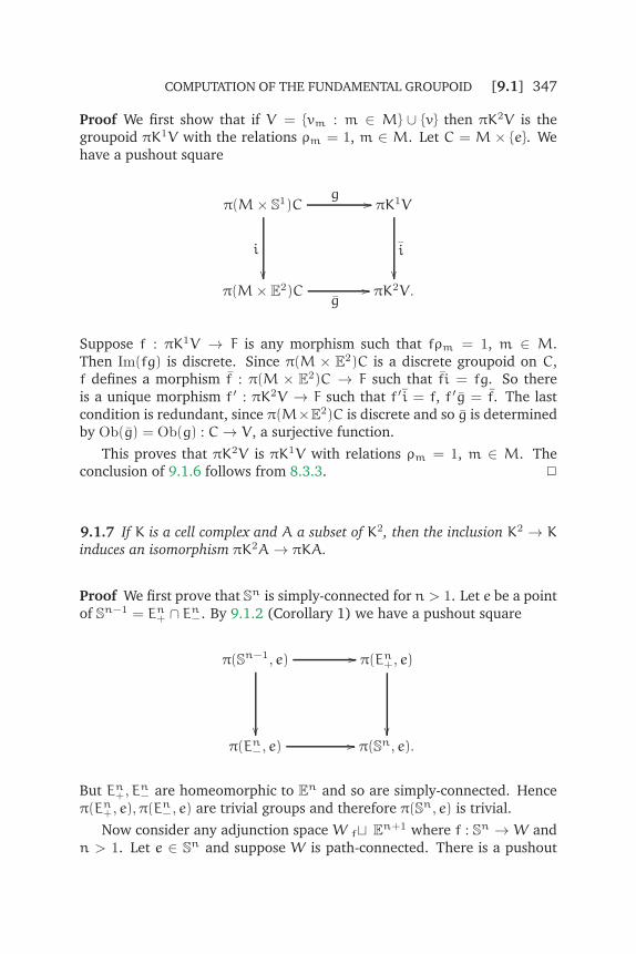
COMPUTATION OF THE FUNDAMENTAL GROUPOID [9.1] 347
Proof We first show that if V = {vm : m ∈ M} ∪ {v} then πK2V is thegroupoid πK1V with the relations ρm = 1, m ∈ M. Let C = M × {e}. Wehave a pushout square
π(M× S1)Cg //
i
��
πK1V
i
��π(M× E2)C
g// πK2V .
Suppose f : πK1V → F is any morphism such that fρm = 1, m ∈ M.Then Im(fg) is discrete. Since π(M × E2)C is a discrete groupoid on C,f defines a morphism f : π(M × E2)C → F such that fi = fg. So thereis a unique morphism f ′ : πK2V → F such that f ′ i = f, f ′g = f. The lastcondition is redundant, since π(M×E2)C is discrete and so g is determinedby Ob(g) = Ob(g) : C→ V , a surjective function.
This proves that πK2V is πK1V with relations ρm = 1, m ∈ M. Theconclusion of 9.1.6 follows from 8.3.3. ✷
9.1.7 If K is a cell complex and A a subset of K2, then the inclusion K2 → Kinduces an isomorphism πK2A→ πKA.
Proof We first prove that Sn is simply-connected for n > 1. Let e be a pointof Sn−1 = En+ ∩ En−. By 9.1.2 (Corollary 1) we have a pushout square
π(Sn−1, e) //
��
π(En+, e)
��π(En−, e)
// π(Sn, e).
But En+,En− are homeomorphic to En and so are simply-connected. Hence
π(En+, e),π(En−, e) are trivial groups and therefore π(Sn, e) is trivial.
Now consider any adjunction space W f⊔ En+1 where f : Sn → W andn > 1. Let e ∈ Sn and suppose W is path-connected. There is a pushout

348 [9.1] TOPOLOGY AND GROUPOIDS
square
π(Sn, e)f //
i
��
π(W, fe)
i
��π(En+1, e)
f// π(W f⊔ En+1, fe).
Since the two left-hand groups are trivial, i is an isomorphism. ✷
In order to compute the fundamental group of spaces, it is clearly neces-sary to compute maps π(S1, e)→ π(K1, fe). The following result is crucial.
9.1.8 Let f : S1 → S1 be the map z 7→ zn, n an integer. Then the induced
morphism f : π(S1, e)→ π(S1, e) of additive groups is multiplication by n.
Proof The result is clearly true if n = 0, since f is then constant, or if n = 1,since f is then the identity. Suppose n > 1; let w be the complex numbere2πi/n and let wr = e2πir/n, r = 0, 1, . . . ,n − 1. Let Xr be the subset of S1
of points e2πiθ, r/n 6 θ 6 (r + 1)/n, let Cr consist solely of wr,wr+1 andlet C = {wr : 0 6 r < n}. Since Xr is simply-connected there is a uniqueelement ır in πXr(w
r,wr+1). The morphism πXrCr → πS1C induced byinclusion is injective and so we regard πXrCr as a subgroupoid of πS1C. Agenerator a of π(S1, e) where e = w0, is then given by
a = ın−1 + · · ·+ ı0.
The map f : S1 → S1 determines by restriction f ′ : Xr → S1; clearlyf ′ır = a. Therefore,
fa = f(ın−1 + · · · + ı0) = a+ · · ·+ a = na.
If n < 0, let m = −n. The z 7→ zn is the composite of g : z 7→ z−1 andz 7→ zm. But if b : I→ S1 is the path t 7→ e2πit, then gb is t 7→ e−2πit, thatis, gb = −b. Hence, in π(S1, e), ga− fa; therefore fa = −ma = na. ✷
If f : S1 → S1 is a map such that f : π(S1, 1)→ π(S1, 1) is multiplicationby n, then we say f is of degree n.
EXAMPLES
1. Let K = S1 ∨ · · · ∨ S1 be a wedge of n circles, with the cell structuree0 ∪ e11 ∪ · · · ∪ e1n. Let v be the vertex of K. Then π(K, v) is a free group onn-generators, the generators being the classes of the loops which pass onceround one of the circles.

COMPUTATION OF THE FUNDAMENTAL GROUPOID [9.1] 349
2. The fundamental group of the real projective plane P2(R) and the realprojective n-space Pn(R) (n > 1) are the same, by 9.1.7 and the fact thatP2(R) can be identified with the 2-skeleton of Pn(R). Also, P2(R) = S1 f⊔E2 where f : S1 → S1 is of degree 2 [Section 5.3]. It follows that thefundamental group of P2(R) is the group Z/2Z = Z2.3. We can also state that the fundamental groups of S2 and S1 × S1 are 0
and Z × Z respectively. It follows that no two of the spaces S2, S1 × S1,Pn(R) are of the same homotopy type; a fortiori, no two of these spaces arehomeomorphic.4. The Klein bottle has a cell structure K = e0 ∪ e11 ∪ e12 ∪ e2. From Fig. 4.4,p. 98, it is clear that, if {a,b} is a set of generators of π(K1, v) as givenin 9.1.5, then the relation determined by the 2-cell of K is abab−1. Thusπ(K, v) is a free group on two generators a,bwith the relation abab−1 = 1.
It is a simple consequence of 9.1.2 that if we form a pushout of spacesQ = B f⊔ (X × I) by attaching a cylinder X × I to B by means of a mapf : X × I → B then the fundamental groupoid of Q, on an appropriateset, may be described as a pushout of groupoids in a manner analogous to(8.4.2). We leave the reader to describe this precisely.
The last result on HNN-extensions, and our earlier proofs that that thefundamental group of a circle is infinite cyclic, show that some groups arewell described as constructed from groupoids. On the other hand, it issometimes convenient to regard groups as object groups of groupoids. Asan example, consider the trefoil group Tr = gp〈x,y | x3y−2〉. This is knownto be an infinite group, but from this viewpoint it is not so easy to find anormal form for its elements.
A different way into its structure comes from seeing the trefoil group asa fundamental group of a cell complex given as a double mapping cylinder.Let the unit circle S1 have base point e, say, and consider the double map-ping cylinder M = M(3, 2) of the maps S1 → S1 given by z 7→ z3, z 7→ z2
respectively. This spaceM contains two copies of S1 with base points e3, e2,say. Let E be the set of these base points. Then the fundamental groupoid
T = π(M,E) has a presentation with three generators x ∈ T(e3), y ∈ T (e2),w ∈ T(e3, e2) with the relation wx3 = y2w. An advantage of this ‘Trefoil
groupoid’ T over the Trefoil group Tr is that the generator w acts as a kindof ‘separator’ of the generators x, y for any well defined word in these gen-erators not containing consecutive symbols u,u−1, for u = x,y,w or theirinverses. For this reason, it is easy to give a normal form for words, and weleave this as an exercise for the reader.
Notice also that the double mapping cylinder M as above is a cell com-plex. By contrast, the pushout P of the two maps S1 → S1 as above is noteven Hausdorff, and it is not clear what might be its fundamental groupoid.

350 [9.1] TOPOLOGY AND GROUPOIDS
By contrast, the groupoid T is easily understood: it is the double mappingcylinder in the category of groupoids of the two morphisms Z → Z givenby multiplication by 2 and by 3 respectively.
We now give an intuitive account of the computation of the fundamentalgroup of the complement of a graph embedded in Euclidean space R3. Thiscomputation is important in knot theory.
By a graph in R3 we mean a cell complex K of dimension 1 which isembedded in R3. Such a graph is usually represented by a diagram withvertices, overpasses, edges and crossings as in Fig. 9.3.
v
u
zx
y
Fig. 9.3
In order to avoid wildness problems, for example edges which wind in-finitely often round others (see [FA49]) we suppose given a 1-dimensionalcomplex K and an embedding i : K × E2 → R3. That is, the edges of thegraph are taken to have a certain thickness.
The diagram D of the embedding can be regarded as the projection ofi[K× E2] onto R2 by the mapping (x,y, z) 7→ (x,y), and it is supposed thatthe embedding is arranged so that the diagram has edges crossing onlyat double points. This conforms with our picture. The diagram allows usto divide the embedded graph into vertices, namely the images of v × E2
where v is a vertex of K at which more than two edges meet, and overpasses,namely the edges between vertices, between crossings, or between verticesand crossings. Thus the overpasses are labelled by letters in Fig. 9.3. Wealso orient the graph by choosing a direction for each overpass as shown.
9.1.9 Under the above circumstances, the fundamental group π(R3 \ i[K ×E2],p) has a presentation with a generator for each overpass and relations of
two types:
(a) at each vertex v there is a relation xε1
1 xε2
2 . . . xεrr = 1, where the xi are the
edges at the vertex and the sign εi is +1 if the arrow for xi points towards the
vertex, and −1 otherwise;

COMPUTATION OF THE FUNDAMENTAL GROUPOID [9.1] 351
(b) at each crossing with overpass x crossing y and z as shown in Fig. 9.4 (ii),there is a relation y = xzx−1.
(i) (ii)
xy
z
Fig. 9.4
A proof goes roughly as follows. Imagine the graph i[K× E2] as part ofa slice S = R2× [−ε, ε] of R3, while S is regarded as the intersection of twohalf spaces H+ = R2× [−ε,→[ and H− = R2× ]←, ε]. Surround each vertexv by a solid ball Ev and each crossing c by a solid ball Dc as in Fig. 9.5.
Ev Dc
Fig. 9.5
Let X be the union of i[K × E2] and all the balls Ev and Dc. Arrange theseso that H+ \ X and H− \ X intersect in a non connected space with onecomponent for each region into which the diagram of the graph divides theplane. By 6.7.2 and 8.4.1, the fundamental group R3 \ X is a free groupwith one generator for each edge ei of the diagram between crossings orvertices. Now replace the balls Ev and Dc with their intersection withi[K× E2] excised. It is easy to see that Ev contributes a relation as given ateach vertex. The balls Dc contribute two relations. One of these ‘continues’an overpass while the other is the relation we want; that is in the situationshown in Fig. 9.6,
xi
xl
xm
xj
Fig. 9.6
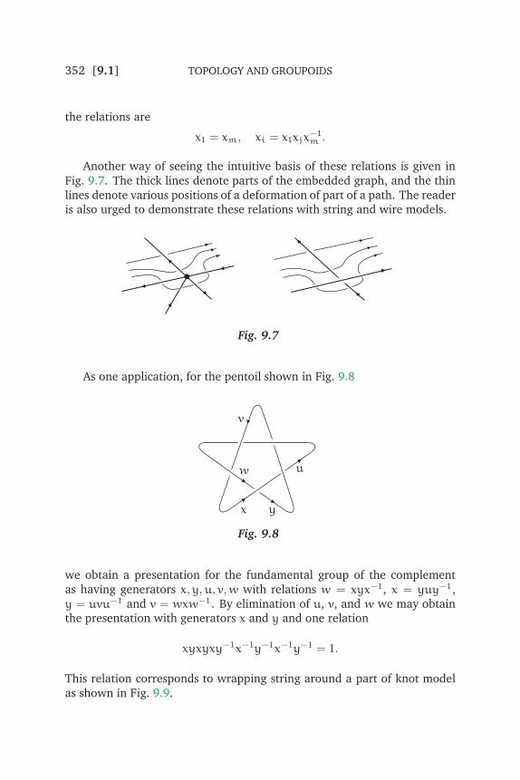
352 [9.1] TOPOLOGY AND GROUPOIDS
the relations are
xl = xm, xi = xlxjx−1m .
Another way of seeing the intuitive basis of these relations is given inFig. 9.7. The thick lines denote parts of the embedded graph, and the thinlines denote various positions of a deformation of part of a path. The readeris also urged to demonstrate these relations with string and wire models.
Fig. 9.7
As one application, for the pentoil shown in Fig. 9.8
v
w u
x y
Fig. 9.8
we obtain a presentation for the fundamental group of the complementas having generators x,y,u, v,w with relations w = xyx−1, x = yuy−1,y = uvu−1 and v = wxw−1. By elimination of u, v, and w we may obtainthe presentation with generators x and y and one relation
xyxyxy−1x−1y−1x−1y−1 = 1.
This relation corresponds to wrapping string around a part of knot modelas shown in Fig. 9.9.

COMPUTATION OF THE FUNDAMENTAL GROUPOID [9.1] 353
x
y
Fig. 9.9
If you wrap string around a model of the pentoil in precisely this way, andthen tie the ends together, the loop will disentangle itself from the knot,thus demonstrating the calculation. (See [Bro88].)
For further information on knots and links, consult also [Kau87]. Forrelations of the fundamental group to the important area of configurationspaces (these are spaces of n distinct points in a space X) see also [Bir75].
EXERCISES
1. Prove that 9.1.7 is a consequence of the cellular approximation theorem.
2. Prove that the spaces Pn(H) are simply-connected.
3. Prove that S1 is not a retract of Pn(R), n > 1.
4. Let X = Y ∪ Z where Z, Y are path-connected and (X,Y) is cofibred. Let
a0,a1, . . . ,an be points one in each path-component of Y ∩ Z. Let i, j be the in-
clusions of Y ∩ Z into Y,Z respectively. Let αr ∈ πY(a0,ar), βr ∈ πZ(a0,ar),
r = 0, . . . ,n, with α0 = 1, β0 = 1. Let F be a free group on elements γr, r = 0, . . . ,n
with the relation γ0 = 1. Prove that π(X,a0) is isomorphic to the free product of
the groups π(Y,a0), π(Z,a0) and F with the relations
α−1r (iρr)αr = γr(β
−1r (jρr)βr)γ
−1r
for all ρr ∈ π(Y ∩ Z,ar) and r = 0, . . . ,n. [Here γr corresponds to the element
(uβ−1r )(vαr) of π(X,a0) where u, v are the inclusions of Y,Z respectively into X.]
5. Let K,L be 1-dimensional (finite) cell complexes. Prove that if ϕ : πKK0 → πLL0
is any morphism, then there is a map f : K → L such that πf = ϕ. Prove also
that if f, g : K → L are cellular maps such that πf ≃ πg : πKK0 → πLL0, then f is
homotopic to g.
6. Extend the results 9.1.5, 9.1.6, 9.1.7 to (infinite) CW-complexes. Prove that if G
is any group, then there is a CW-complex K and a vertex x of K such that π(K,x) is
isomorphic to G. Deduce that if G is any groupoid then there is a CW-complex K
such that πKK0 is isomorphic to G. [You may assume that if G is any group then
there is a free group F and a free subgroup R of F such that G is isomorphic to F/R.]
7. Prove that R2 and Rn for n > 2 are not homeomorphic.
354 [9.2] TOPOLOGY AND GROUPOIDS
8. Let p : z 7→ zn + an−1zn−1 + · · · + a1z+ a0 and q : z 7→ zn be polynomials with
ai ∈ C. For r > 0 let Cr = {z ∈ R2 : |z| = r}. Prove that for r large enough, p and q
restrict to homotopic maps Cr → R2 \ {0}. Prove that for any r > 0 this restriction
of q is essential and hence show that the polynomial p has a root. [This is known
as the Fundamental Theorem of Algebra.]
9.2 The Jordan Curve Theorem
The Jordan Curve Theorem states that if C is a subset of the plane R2
such that C is homeomorphic to the circle S1, then R2 \ C has exactly twocomponents, one of them bounded and the other unbounded, and eachwith C as boundary. The set C is called a simple closed curve in R2. Thebounded component of R2 \ C is of course called the inside of the curve,and the unbounded component is called the outside of the curve.
This theorem is a classic instance of a result which at first sight seemsintuitively obvious, but which needs some sophisticated machinery for itsproof. In fact the theorem is not quite so obvious intuitively. Considerfor example the computer generated simple closed curve in R2 shown inFig. 9.10. How do you determine the inside and outside? (I am indebtedto S. J. Abas for this diagram.)
Any method you choose for this curve might be defeated by a morecomplicated example. In any case, if you try and work out the inside andoutside for this case, you begin to see the prospective complications of theproblem.
In this section we shall use the final results of the last section to give acomplete proof of the theorem; we also draw further consequences of themethod. For this reason, we take what might seem a circuitous route to thetheorem, by introducing a property which a space may or may not have.

COMPUTATION OF THE FUNDAMENTAL GROUPOID [9.2] 355
Fig. 9.10
A topological space X is said to have the Phragmen-Brouwer property
(here abbreviated to PBP) if X is connected and the following holds: if D
and E are disjoint, closed subsets of X, and if a and b are points in X\ (D∪E)which lie in the same component of X\D and in the same component of X\E,
then a and b lie in the same component of X \ (D ∪ E). To express this moresuccinctly, we say a subset D of a space X separates the points a and b if aand b lie in distinct components of X \D. Thus the PBP is that: if D and Eare disjoint closed subsets of X and a,b are points of X not in D ∪ E suchthat neither D nor E separate a and b, then D ∪ E does not separate a andb1 .
A standard example of a space not having the PBP is the circle S1, sincewe can take D = {+1}, E = {−1}, a = i, b = −i. This example is typical,as the next result shows. But first we remark that our criterion for thePBP will involve fundamental groups, that is will involve paths, and so weneed to work with path-components rather than components. However,if X is locally path-connected, then components and path-components ofopen sets of X coincide, and so for these spaces we can replace in the PBP‘component’ by ‘path-component’. This explains the assumption of locallypath-connected in the results that follow.
1Some corrections to this Section and to a published paper are given inhttps://arxiv.org/abs/1404.0556

356 [9.2] TOPOLOGY AND GROUPOIDS
9.2.1 Let X be a path-connected and locally path-connected space whose fun-damental group (at any point) does not have the integers Z as a retract. Then
X has the PBP.
Proof Suppose X does not have the PBP. Then there are disjoint, closedsubsets D and E of X and points a and b of X \ (D ∪ E) such that D ∪ Eseparates a and b but neither D nor E separates a and b. Let X1 = X \D,X2 = X \ E, X0 = X \ (D ∪ E) = X1 ∩ X2. Let J be a subset of X0 suchthat a,b ∈ J and J meets each path-component of X0 in exactly one point.Since D and E do not separate a and b, there are elements α ∈ πX1(a,b)
and β ∈ πX2(a,b). Since X is path-connected, the set J is representative inX0, X1 and X2. By 6.7.2 the following diagram of morphisms induced byinclusions is a pushout of groupoids:
πX0Ji1 //
i2
��
πX1J
u1
��πX2J u2
// πXJ.
Since X1 and X2 are path-connected and J has more than one element, itfollows from (8.4.1) (Corollary) that πXJ has the integers Z as a retract. ✷
As an immediate application we obtain:
9.2.2 The following spaces have the PBP: the sphere Sn for n > 1; S2 \ {a}
for a ∈ S2; Sn \A if A is a finite set in Sn and n > 2. ✷
In each of these cases the fundamental group is trivial.An important step in our proof of the Jordan Curve Theorem is to show
that if A is an arc in S2, that is a subspace of S2 homeomorphic to the unitinterval I, then the complement of A is path-connected. This follows fromthe following more general result.
9.2.3 Let X be a path-connected and locally path-connected Hausdorff spacesuch that for each x in X the space X \ {x} has the PBP. Then any arc in X has
path-connected complement.
Proof Suppose A is an arc in X and X \A is not path-connected. Let a andb lie in distinct path-components of X \A.
By choosing a homeomorphism I→ A we can speak unambiguously ofthe mid-point of A or of any subarc of A. Let x be the mid-point of A, sothat A is the union of sub-arcs A ′ and A ′′ with intersection {x}. Since X is
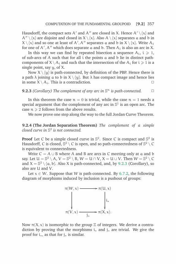
COMPUTATION OF THE FUNDAMENTAL GROUPOID [9.2] 357
Hausdorff, the compact sets A ′ and A ′′ are closed in X. Hence A ′ \ {x} andA ′′ \ {x} are disjoint and closed in X \ {x}. Also A \ {x} separates a and b inX \ {x} and so one at least of A ′,A ′′ separates a and b in X \ {x}. Write A1
for one of A ′,A ′′ which does separate a and b. Then A1 is also an arc in X.
In this way we can find by repeated bisection a sequence Ai, i > 1,of sub-arcs of A such that for all i the points a and b lie in distinct path-components of X \Ai and such that the intersection of the Ai for i > 1 is asingle point, say y, of X.
Now X \ {y} is path-connected, by definition of the PBP. Hence there isa path λ joining a to b in X \ {y}. But λ has compact image and hence liesin some X \Ai. This is a contradiction. ✷
9.2.3 (Corollary) The complement of any arc in Sn is path-connected. ✷
In this theorem the case n = 0 is trivial, while the case n = 1 needs aspecial argument that the complement of any arc in S1 is an open arc. Thecase n > 2 follows from the above results.
We now prove one step along the way to the full Jordan Curve Theorem.
9.2.4 (The Jordan Separation Theorem) The complement of a simple
closed curve in S2 is not connected.
Proof Let C be a simple closed curve in S2. Since C is compact and S2 isHausdorff, C is closed, S2 \ C is open, and so path-connectedness of S2 \ Cis equivalent to connectedness.
Write C = A ∪ B where A and B are arcs in C meeting only at a and bsay. Let U = S2 \ A, V = S2 \ B, W = U ∩ V , X = U ∪ V . Then W = S2 \ Cand X = S2 \ {a,b}. Also X is path-connected, and, by 9.2.3 (Corollary), soalso are U and V .
Let x ∈ W. Suppose that W is path-connected. By 6.7.2, the followingdiagram of morphisms induced by inclusion is a pushout of groups:
π(W, x) //
��
π(U, x)
i∗
��π(V , x)
j∗// π(X, x).
Now π(X, x) is isomorphic to the group Z of integers. We derive a contra-diction by proving that the morphisms i∗ and j∗ are trivial. We give theproof for i∗, as that for j∗ is similar.

358 [9.2] TOPOLOGY AND GROUPOIDS
Let f : S1 → U be a map and let g = if : S1 → X. Choose a homeomor-phism h : S2 \ {a} → R2 which takes b to 0 and such that hg maps S1 intoR2 \ {0}. Since hg[S1] is compact, there is only one unbounded componentof R2\g[S1], and we may assume this contains 0. Again since hg[S1] is com-pact, there is an r > 0 such that hg[S1] ⊆ B(0, r). Choose a point y in R2
such that ‖y‖ > r. Then there is a path λ, say, joining 0 to y in R2 \ hg[S1],since 0 lies in the unbounded component of this set.
Define G : S1 × I→ R2 by
G(z, t) =
{hg(z) − λ(2t) if 0 6 t 6 1
2,
(2− 2t)hg(z) − y if 126 t 6 1.
Then G is well-defined. Also G never takes the value 0 (this explains thechoices of λ and y). So G gives a homotopy in R2 \ {0} from hg to theconstant map at −y. So hg is inessential and hence g is inessential. Thiscompletes the proof that i∗ is trivial. ✷
As we shall see, the Jordan Separation Theorem is used in the proof ofthe Jordan Curve Theorem.
9.2.5 (Jordan Curve Theorem) If C is a simple closed curve in S2, then the
complement of C has exactly two components, each with C as boundary.
Proof As in the proof of 9.2.4, write C as the union of two arcs A and Bmeeting only at a and b say, and let U = S2 \ A, V = S2 \ B. Then U andV are path-connected and X = U ∪ V = S2 \ {a,b} has fundamental groupisomorphic to Z. AlsoW = U∩V = S2\C has at least two path-components,by 9.2.4.
IfW has more than two path-components, then the fundamental groupG of X contains a copy of the free group on two generators, by 8.4.1 (Corol-lary), and so G is non-abelian. This is a contradiction, since G ∼= Z. So Whas exactly two path-components P and Q, say, and this proves the firstpart of 9.2.5.
Since C is closed in S2 and S2 is locally path-connected, the sets P andQ are open in S2. It follows that if x ∈ P \ P then x /∈ Q, and hence P \ P iscontained in C. So also is Q \Q, for similar reasons. We prove these setsare equal to C.
Let x ∈ C and let N be a neighbourhood of x in S2. We prove N meetsP \ P. Since P \ P is closed and N is arbitrary, this proves that x ∈ P \ P.
Write C in a possibly new way as a union of two arcs D and E intersect-ing in precisely two points and such that x is in the interior with respect toD of D. Choose points p in P and q in Q. Since S2 \ E is path-connected,there is a path λ joining p to q in S2 \E. Then λ must meetD, since p and q

COMPUTATION OF THE FUNDAMENTAL GROUPOID [9.2] 359
lie in distinct path-components of S2\E. In fact if s = sup{t ∈ I : λ[0, t] ⊆ P},then λ(s) ∈ P \ P. It follows that N meets P \ P.
So P \ P = C and similarly Q \Q = C. ✷
NOTES
There are many books containing a further discussion of this area. For moreon the Phragmen-Brouwer property, see [Why42] and [Wil49].Wilder lists five other properties which he shows for a connected and lo-cally connected metric space are each equivalent to the PBP. The aboveproof of the Jordan Curve Theorem is adapted from [Mun75]; because hedoes not have our Van Kampen theorem for non-connected spaces, he isforced into rather special covering space arguments to prove his replace-ments for 9.1.9 (Corollary) and for 9.2.1. As far as I am aware, 9.2.1 and9.2.2 are not previously published.
A different kind of proof of the Jordan Curve Theorem is given in[Mae84]; this uses only the Brouwer Fixed Point Theorem and the TietzeExtension Theorem.
An important strengthening of the Jordan Curve Theorem is the Schoen-flies Theorem: if C is a simple closed curve in S2 then each component of
S2 \ C is homeomorphic to R2; in fact, there is a homeomorphism h : R2 →R2 which takes C to the standard circle S1. For more information onthis area, see for example [Moi77], [Bin83], [Sie05], and the web sitewww.maths.ed.ac.uk/~aar/jordan/.
For exercises in this area, see [Mun75].An important part of algebraic topology deals with braids, links and
mapping class groups [Bir75], but the results on groupoids given in thisbook have hardly been used in that area.

360 [9.2] TOPOLOGY AND GROUPOIDS

Chapter 10
Covering spaces, covering
groupoids
The notion of a covering space is of interest for several reasons. First, the
construction of a covering space X from a given space X (which we give in
section 10.5) is useful since the structure of X is in a sense simpler than that
of X (X has a ‘smaller’ fundamental group than X). Second, the method ofstudying a given space X by means of particular kinds of maps into X isof wide importance in topology—the covering maps onto X exemplify this,and indeed form a particular example of the fibre maps whose ramifica-tions extend through topology, differential geometry, analysis, and evenalgebra. Third, and most important from the point of view of this book, thetopology is here very nicely modelled in the notion of covering morphismof groupoids. With this account, we give a further aspect of combinatorialgroupoid theory, and one which is important for applications to topologyand to group theory. It may be that the results of the next chapter will alsocome to be seen in this light.
These results also imply that the fundamental group of the circle is in-finite cyclic, and indeed this is the classical method of proof. However thegroupoid viewpoint adds new insight to this and other results.
The main result is the equivalence of categories between the categoryof covering maps of a ‘locally nice’ space X and the category of coveringmorphisms of the fundamental groupoid πX. In this way, we really doshow a tight analogy between topology and algebra. The method of proofgives tighter results than those usually given, and has also been applied toother situations, such as when X is a topological group.
We shall use additive notation for groupoids in this chapter.
361

362 [10.1] TOPOLOGY AND GROUPOIDS
10.1 Covering maps and covering homotopies
Throughout this chapter all spaces will be assumed locally path-connected
(or proved to be so). This assumption is not essential for all the results (foran alternative approach see [HW60] or [Spa66]) but it does seem to leadto a smoother theory; also the study of covering maps for spaces which arenot locally path-connected is something of a curiosity.
Definitions Let p : X→ X be a map of topological spaces. A subset U of Xis called canonical (with respect to p) ifU is open, path-connected, and each
path-component of p−1[U] is open in X and is mapped by p homeomorphi-cally onto U; each path-component of p−1[U] is also called canonical. Themap p is called a covering map if each x in X has a canonical neighbour-
hood; and in such case X is called a covering space of X. The covering map
p is called connected if both X and X are path-connected.
The local picture of a covering map is thus that of Fig. 10.1(a).
}(a)
U
p
p−1[U]
(b)
−1 1
q
Fig. 10.1
EXAMPLES
1. Consider the map p : R→ S1, t 7→ e2πit. The sets
U1 = S1 \ {1}, U−1 = S1 \ {−1}
form an open cover of S1. The path-components of p−1[U1] (respectivelyp−1[U−1]) are open intervals ]n,n+ 1[ (respectively ]n− 1
2,n+ 1
2[ ) for all
n ∈ Z. So p is a covering map. A good picture of p is obtained by writingp = qr where r : R → R2 × R is t 7→ (pt, t) and q : R2 × R → R2 is theprojection. Thus the image of r is the helix of Fig. 10.1(b).

COVERING SPACES, COVERING GROUPOIDS [10.1] 363
2. Let f : S1 → S1 be the map z 7→ zn, where n is a non-zero integer. Itis easily proved by using the sets U1,U−1 of Example 1 that f is a coveringmap.
3. If p : X→ X is a covering map, then for each x in X the subspace p−1[x]
of X is a discrete space—this follows from the fact that if U is a canonical
set then the path-components of p−1[U] are open in X. It follows that thefundamental map p : Rn+1
∗ → Pn(R) is not a covering map.4. However, let i : Sn → Rn+1
∗ be the inclusion so that h = pi is theHopf map. Let Ui be the subset of Pn(R) of points px such that the ithcoordinate of x is non-zero. The sets Ui, i = 1, . . .n+1 form an open coverof Pn(R). The path-components of h−1[Ui] are two open hemispheres of Sn
each of which is mapped homeomorphically by h onto Ui. (For example,h−1[Un+1] = Sn \ Sn−1.) Therefore, h is a covering map.
Let p : X→ X be a covering map. If the diagram of maps
X
p
��Y
f
@@�������������
h// X
is commutative, then we say f is a lifting of h, or that f covers h. We shallsee that the central properties of covering maps are concerned with liftings;for example, we have the following covering homotopy property.
10.1.1 Let p : X → X be a covering map and suppose given a commutative
diagram of maps (in which i is z 7→ (z, 0))
Zf //
i
��
X
p
��Z× [0, r]
H// X
so that H is a homotopy of pf. Then H is covered by a unique homotopy
F : Z× [0, r]→ X of f.
Proof Since Z is locally path-connected, each path-component of Z is openin Z. Therefore, it is sufficient to work in each path-component of Z at atime, that is, to assume Z is path-connected.

364 [10.1] TOPOLOGY AND GROUPOIDS
Step 1. Suppose that ImH is contained in a canonical subset U of X.Since Z is path-connected, Im f is contained in a path-component V ofp−1[U]. Let pV be the inverse of the homeomorphism p | V ,U. Thenthe map
F : Z× [0, r]→ X
(z, t) 7→ pVH(z, t)
is a homotopy of f which covers H. Since Z × [0, r] is path-connected, it isalso the only such homotopy of f.
Step 2. Suppose that the homotopy H is a sum
H = Hn + · · ·+H1
such that the image of each Hi is contained in a canonical subset of X.By Step 1, we can define inductively unique homotopies Fi : fi ≃ fi+1,i = 1, . . . ,n, such that f1 = f and Fi covers Hi. Clearly,
F = Fn + · · ·+ F1
is a homotopy of f which covers H. If F′ is any other homotopy of f whichcovers H, then the given subdivision of H determines a subdivision F′ =
F′n + · · · + F′1. It follows by induction that F′i = Fi, i = 1, . . . ,n and soF′ = F.
Step 3. Let z ∈ Z. We use Step 2 to show that the result is true with Zreplaced by some neighbourhood Mz of z.
For each t in [0, r] there are open neighbourhoodsMt,Nt of z, t respec-tively such that H[Mt×Nt] is contained in a canonical subset of X. The set{Nt : t ∈ [0, r]} is an open cover of [0, r] which, by compactness, has a finitesubcover {Nt : t ∈ A} say. Let
M =⋂
t∈A
Mt
and let Mz be an open path-connected neighbourhood of z contained inM.
Let l be the Lebesgue number of the cover {Nt : t ∈ A} and let n bean integer such that 0 < r/n < l/2. For each i = 1, . . . ,n the intervalLi = [(i − 1)r/n, ir/n] is contained in some Nt, t ∈ A, and so H[Mz × Li]is contained in a canonical subset of X.
Let Hzi be the homotopy
Mz × [0, r/n]→ X
(w, t) 7→ H(w, (i − 1)r/n+ t)

COVERING SPACES, COVERING GROUPOIDS [10.1] 365
and let
Hz = H |Mz × [0, r] = Hzn + · · ·+Hz
1.
By Step 2, Hz is covered by a unique homotopy Fz of f |Mz.
Step 4. Let F : Z × [0, r] → X be the function (z, t) 7→ Fz(z, t). Theuniqueness part of the above argument shows that for each z ∈ Z
F |Mz × [0, r] = Fz.
Since Mz is a neighbourhood of z, it follows that F is continuous. Clearly, Fis the unique homotopy of f covering H. ✷
Our main use of the covering homotopy property is to prove the follow-ing path lifting property.
10.1.2 Let p : X → X be a covering map, let x ∈ X and let x = px. Thenpaths a,b in X with initial point x lift uniquely to paths a, b with initial point
x; and a is equivalent to b if and only if a is equivalent to b.
Proof The existence and uniqueness of a (and also b) is immediate from10.1.1 by taking Z to consist of a single point z and defining
fz = x, H(z, t) = at, t ∈ [0, r], r = |a|.
Suppose next that a,b are paths from x to y of length rwhich are homo-topic rel end points. Then, twisting the usual way of writing a homotopy,there is a map
H : I× [0, r]→ X
such that
H(s, 0) = x, H(s, r) = y, s ∈ I
H(0, t) = at, H(1, t) = bt, t ∈ [0, r].
Let f : I → X be the constant map with value x. Then H is a homotopy ofpf and so, by 10.1.1, H is covered by a unique homotopy F of f.
The paths in X
t 7→ F(0, t), t 7→ F(1, t)
have initial point x and cover a,b respectively; so these paths are a, b re-spectively. The path s 7→ F(s, r) covers the constant path at y and so (byuniqueness) is itself constant; the path s 7→ F(s, 0) is constant by definitionof F. Therefore, F (suitably twisted) is a homotopy rel end points a ≃ b.

366 [10.1] TOPOLOGY AND GROUPOIDS
Finally, if there are real numbers s, s ′ > 0 such that s + a, s ′ + b arehomotopic rel end points, then s+ a, s ′ + b cover s+ a, s ′ + b respectively,and hence a is equivalent to b. ✷
Remark In fact, we shall use only the consequence 10.1.2 of 10.1.1 and not10.1.1 itself. A simpler proof of 10.1.1 can be given in the case Z = [0,q]
by subdividing the rectangle [0,q]× [0, r] into rectangles so small that eachis mapped by H into a canonical subset of X. But the interest of 10.1.1is that, provided the word uniqueness is omitted, it applies to many othersituations. For example, the fundamental map Kn+1
∗ → Pn(K) satisfiesthis weaker covering homotopy property—this follows from Exercise 8 ofSection 5.3 and results of [Dol63] (see also [Spa66, 2.7.12]).
EXERCISES
1. Which of the following maps are covering maps?
(i) R→ R, x 7→ x2.
(ii) R→ R, x 7→ x3.
(iii) R∗ → R∗, x 7→ x2.
(iv) S1 → S1, eiθ 7→ e2i|θ| (−π < θ 6 π).
(v) ]0, 3[→ S1, t 7→ e2πit.
2. Let f : Y ′ → Y, g : X → X ′ be homeomorphisms and let p : Y → X be a covering
map. Prove that gpf : Y ′ → X ′ is a covering map.
3. Let p : X → X be a covering map, let f : Y → X be a map, let i : A → Y be an
inclusion and let G : A× I→ X be a homotopy of f | A. Prove that, if H : Y × I→ X
is a homotopy of pf which agrees with pG on A, then H is covered by a homotopy
F of f such that F extends G. Deduce that for any map u : A → X, p induces an
injection p∗ : [(Y, i), (X,u)]→ [(Y, i), (X,pu)].
4. Prove that 10.1.1 is true without the assumption that Z is locally path-connected.
5. Let p : X→ X be a covering map and let f : Y → X be a map. Let
Xf = {(y, x) ∈ Y × X : fy = px}
and let pf : Xf → Y be the restriction of Xf of the projection Y × X→ Y. Prove that
Xf is locally path-connected. Prove also that pf is a covering map. Prove also that f
lifts to X if and only if there is a map s : Y → Xf such that pfs = 1.
6. Let p : X → X be a covering map and let i : A → X be the inclusion of the
subspace A of X. Prove that if q = p | p−1[A],A then there is a homeomorphism
g : Xi → p−1[A] such that qg = pi (where Xi,pi are as in the previous exercise).
7. Let G be the sheaf of germs of continuous functions from R to R [Exercise 3 of
Section 2.10]. Prove that the projection p : G → R, fx 7→ f(x), is not a covering
map.

COVERING SPACES, COVERING GROUPOIDS [10.2] 367
8. Give another proof of 10.1.1 on the following lines. First prove it is true when Z
consists of a single point. In the general case, we then have that for each z in Z then
map H | {z}× [0, r] lifts to a homotopy F | {z}× [0, r] of f | {z}. So we have a function
F : Z× [0, r]→ X. Prove that F is continuous by supposing that F is non-continuous
and obtaining a contradiction by considering the infinum of the set of t such that F
is not continuous at some (z, t).
9. Let p : X → X be a connected covering map which is non-trivial (i.e., it is not
a homeomorphism). Let Y = X × X × X × · · · be the countable product of X with
itself, and let Xn be the n-fold product of X with itself. Let Yn = Xn × Y. Define
pn : Yn → Y by (x1, . . . , xn,x1, x2, . . . ) 7→ (px1, . . . ,pxn, x1, x2, . . . ). Prove that pnis a covering map. Let
Z = ⊔n>1Yn
and let Z be the countably infinite topological sum of Y with itself. Let q = ⊔pn :
Z→ Z and let r : Z→ Y be the obvious projection. Prove that q and r are covering
maps but that the composite rq is not a covering map.
10.2 Covering groupoids
In this section we shall show how covering spaces are modelled in the cat-egory of groupoids.
Let G be a groupoid. For each object x of G the star of x in G, denotedby StG x, is the union of the sets G(x,y) for all objects y of G. Thus StG x
consists of all elements of G with initial point x. When no confusion willarise we abbreviate StG x to St x.
Definition Let p : G → G be a morphism of groupoids. We say p is a
covering morphism if for each object x of G the restriction of p
StGx→ StG px
is bijective; in such case, we call G a covering groupoid of G. The covering
morphism p is called connected if both G and G are connected.
For any morphism p : G → G and object x of G we call the subgroup
p[G(x)] of G(px) the characteristic group of p at x—by an abuse of lan-
guage, we also refer to this group as the characteristic group of G, x. If p
is a covering morphism, then p maps G(x) isomorphically onto this charac-teristic group; also, if a ∈ G(px), then there is a unique element a of St x
such that pa = a, but a will be a loop, that is a will belong to G(x), if and
only if a itself belongs to the characteristic group of G, x.
The sense in which a characteristic group of a covering morphism p
characterises p will be discussed later.

368 [10.2] TOPOLOGY AND GROUPOIDS
EXAMPLES
1. Recall that I is a simply-connected groupoid with two objects 0, 1 andone element ı of I(0, 1). If 0 denotes ambiguously the zero of I at 0 or 1, wehave
StI 0 = {0, ı}, StI 1 = {0,−ı}.
In the group Z2 (which has one object 0 say)
StZ20 = {0, 1}.
Hence if p : I → Z2 is the unique morphism such that pı = 1, then p is acovering morphism. Also each characteristic group of p is trivial.2. In the group Z3 (with one object 0)
StZ30 = {0, 1,−1}.
Hence, although the morphism p : I→ Z3 which sends ı to 1 and −ı to −1
is surjective on the elements, p is not a covering morphism.3. For groups, the only covering morphisms are isomorphisms.
We now show the utility for topology of covering morphisms.
10.2.1 Let p : X → X be a covering map, let A be a subset of X and let
A = p−1[A]. Then the induced morphism
πp : πXA→ πXA
is a covering morphism.
Proof Let x ∈ A and let px = x. For each path a in Xwith initial point x, let
a denote the unique covering path of X with initial point x. If the final point
of a is in A, then the final point of a is in A. Also, the equivalence class ofa depends only on the equivalence class of a (by 10.1.2). So the functionclsa 7→ cls a is inverse to the restriction of p which maps St x 7→ St x. ✷
Once more we obtain:
10.2.1 (Corollary 1) The circle S1 has fundamental group isomorphic to the
integers Z.
Proof Let p : R→ S1 be the covering map t 7→ e2πit so that
p ′ = πp : πRZ→ π(S1, 1)
is a covering morphism. Now πRZ is 1-connected: so for each n ∈ Z thereis a unique element τn of πR(0,n). Of course, τ1 is represented by the pathI → R, t 7→ t, while τn+1 − τn—the unique element of πR(n,n + 1)—is

COVERING SPACES, COVERING GROUPOIDS [10.2] 369
represented by the path I→ R, t 7→ t+ n. It follows from the definition ofp that
p ′(τn+1 − τn) = p′τ1.
Hence, if τ = p ′τ1, then
p ′τn = p ′(τn − τn−1) + · · · + p ′(τ2 − τ1) + p′τ1
= nτ.
Since p ′ is a covering morphism, p ′τn 6= 0, and so
nτ 6= 0.
Also, if a ∈ π(S1, 1), then a = p ′τn for some n and hence
a = nτ.
This shows that π(S1, 1) is an infinite cyclic group with generator τ. ✷
10.2.1 (Corollary 2) For n > 1, real projective n-space Pn(R) has fundamen-
tal group isomorphic to Z2.
Proof The Hopf map h : Sn → Pn(R) is a covering map, and by the proofof 9.1.7 Sn is 1-connected for n > 1. Let x,−x be antipodal points of Sn
and let x = hx = h(−x). By 10.2.1, the morphism
πh : πSn{x,−x}→ π(Pn(R), x)
is a covering morphism. However, the groupoid πSn{x,−x} is isomorphicto I. It follows that the group π(Pn(R), x) has two elements, and so isisomorphic to Z2. ✷
We give in this section some simple results on covering groupoids.
10.2.2 Let p : G→ G be a covering morphism such that G is connected. If a,
b are any elements of G, then p−1[a], p−1[b] have the same cardinality.
Proof Suppose c ∈ G(x,y). It is an easy deduction from the definition ofcovering morphism that the functions
p−1[c]→ p−1[x], p−1[c]→ p−1[y]
which send an element of p−1[c] to its initial and its final point respectively,are both bijections.
Suppose now a ∈ G(x, x1), b ∈ G(y,y1). Since G is connected, there isan element c in G(x,y) and we deduce
||||
p−1[a] = ||||
p−1[x] = ||||
p−1[y] = ||||
p−1[b].

370 [10.2] TOPOLOGY AND GROUPOIDS
✷
In particular, if p−1[a] has n elements for each a in G, then we call pan n-fold covering morphism. We shall see later that for connected coveringmorphisms, this number n is the index in G(px) of the characteristic group
of p at x (x ∈ Ob(G)).
10.2.3 Let r : K → H, q : H → G be morphisms of groupoids. If q and r
are covering morphisms, so also is qr. If q and qr are covering morphisms, so
also is r. If r and qr are covering morphisms and Ob(r) is surjective, then qis a covering morphism.
Proof Let x ∈ Ob(K) and consider the composite (qr)′ = q′r ′
StK xr′
−→ StH rxq′
−→ StG qrx
where q′, r ′ are induced by q, r. Clearly, if any two of q′, r ′, and q′r ′ arebijections, then so is the third. For the last part one needs that any y inOb(H) is rx for some x. ✷
It is not hard to prove for spaces the result corresponding to the onepart of 10.2.3. The other part is more tricky (it is false in general) and willbe left till an exercise in section 10.5.
10.2.4 If r : Z → Y, q : Y → X are maps of spaces such that qr and q are
covering maps, then r is a covering map.
Proof Let x ∈ X, let U be a canonical neighbourhood of x for the map q,and let V be a canonical neighbourhood of x for the map qr. Let W be anopen, path-connected neighbourhood of x contained in U ∩ V . Clearly, Wis canonical for both q and qr (since any open, path-connected subset of acanonical set is again canonical).
For each y in q−1[x], let Wy be the path-component of q−1[W] whichcontains y—these sets Wy are disjoint and open in Y. Clearly,
r−1q−1[W] =⋃
{r−1[Wy] : y ∈ q−1[W]}
and the sets r−1[Wy] are disjoint and open in Z. Therefore, each path-component W ′ of r−1[Wy] is also a path-component of r−1q−1[W]. Butqr |W ′,W and q |Wy,W are homeomorphisms. Therefore r |W ′,Wy is ahomeomorphism. ✷

COVERING SPACES, COVERING GROUPOIDS [10.3] 371
EXERCISES
1. Let f : S1 → S1 be the map z 7→ zn, where n is a non-zero integer. Prove that the
induced map πf : π(S1, 1)→ π(S1, 1) is multiplication by n.
2. Let p : G → G be a covering morphism. Prove that if G is connected and G is
non-empty then Ob(p) is surjective.
3. Prove that a 1-fold covering morphism is an isomorphism.
4. Let p : X→ X be a covering map of spaces such that X is path-connected. Prove
that the sets p−1[x] have the same cardinality for all x in X, and that if X is non-
empty then p is surjective.
5. Let r : Z→ Y, q : Y → X be covering maps such that q−1[x] is finite for each x in
X. Prove that qr is a covering map.
6. Show that the notion of covering morphism for groupoids extends to functors
of categories in such a way that if p : X → X is a covering map of spaces, then
Pp : PX→ PX is a covering functor of categories.
10.3 On lifting sums and morphisms
Let p : G → G be a covering morphism. Because of the analogy with the
fundamental groupoid of covering spaces, we say that an element a of G
covers, or is a lifting, of pa; similarly, we say a sum an+ · · ·+a1 in G covers,or is a lifting, of pan+ · · ·+pa1. The basic property of covering morphisms
is that not only elements of G but also sums in G can be lifted into G.
10.3.1 Let x be an object of G and let px = x. If
a = an + · · · + a1
belongs to St x, then there are unique elements an, . . . , a1 of G such that
(a) pai = ai, i = 1, . . . ,n
(b) a = an + · · ·+ a1 is defined and belongs to St x.
Proof Since p : St y → Stpy is bijective for each object y of G, the ele-ments ai are uniquely defined by the inductive conditions (i) pai = ai, (ii)a1 ∈ St x, (iii) ai ∈ St xi where x1 = x and xi is the final point of ai−1 fori > 1. ✷
As mentioned in the last section, the characteristic group of G, x (that is,
the subgroup p[G(x)] of G(px)) plays an important rule in the theory. Therelationship of these groups for various x is described in the next result.
First we need a definition: subgroups C of G(x), D of G(y) are calledconjugate (in G) if there is an element c of G(x,y) such that
c+ C− c = D.

372 [10.3] TOPOLOGY AND GROUPOIDS
This relation implies easily that −c+D+ c = C.
10.3.2 Let C be the characteristic group of G, x.
(a) If D is the characteristic group of G, y, and x, y lie in the same component
of G, then C and D are conjugate.
(b) If D is a subgroup of G(y) and D is conjugate to C, then D is the charac-
teristic group of G, y for some y.
Proof (a) Let a be an element of G(x, y) and let a = pa. If c ∈ C, then
c is covered by an element c of G(x). By 10.3.1, a + c − a is covered by
a + c − a, which is an element of G(y). Therefore a+ c− a belongs to D.This proves (a).
(b) Suppose a + C − a = D where a ∈ G(x,y). Let a be an element ofSt x covering a, let y be the final point of a, and let D ′ be the characteristic
group of G, y. We prove that D = D ′.
If d ∈ D, then d = a + c − a, where c ∈ C. It follows that d is coveredby an element a + c − a of G(y), whence d ∈ D ′. Conversely, if d ∈ D ′,
then d is covered by an element d of G(y), whence d = a + c − a wherec = p(−a+ d+ a) ∈ C. ✷
We shall now show the sense in which the characteristic group of G, x is
characteristic. It is convenient to work in the category of pointed groupoids:a pointed groupoidG, x consists of a groupoidG and object x ofG. A pointed
morphism G, x → H,y of pointed groupoids consists of G, x and H,y anda morphism f : G → H such that fx = y; such a pointed morphism isusually called a morphism G, x → H,y and is often denoted simply byf. The characteristic group of a pointed morphism f : G, x → H,y is thecharacteristic group of f at x.
If p : G, x → G, x is a pointed morphism, then we say p is a covering
morphism if the morphism p : G → G is a covering morphism. Similarly, ifwe are given a commutative diagram of pointed morphisms
G, x
p
��F, z
f
>>⑤⑤⑤⑤⑤⑤⑤⑤⑤⑤⑤⑤⑤
f// G, x
then we say f is a lifting of f.

COVERING SPACES, COVERING GROUPOIDS [10.3] 373
10.3.3 Let p : G, x → G, x be a covering morphism, and f : F, z → G, x a
morphism such that F is connected. Then f lifts to a morphism f : F, z→ G, xif and only if the characteristic group of f is contained in that of p; and if this
lifting exists, then it is unique.
Proof Suppose first that f exists; the relation pf = f implies
f[F(z)] ⊆ p[G(x)]
and this proves the necessity of the condition.
Suppose, conversely, that the characteristic group of f is contained in the
characteristic group C of p. Since p restricts to an isomorphism G(x)→ C,the morphism
f : F(z)→ G(x)
lifts uniquely to a morphism
f : F(z)→ G(x).
For each object v of F let τv be an element of F(z, v) (with τz = 0). Ifa ∈ F(u, v) then a can be written uniquely as
a = τv + a′ − τu
with a ′ ∈ F(z); and if, further, b ∈ F(v,w), then (b + a)′ = b ′ + a ′. Noweach element fτv is covered by a unique element fτv of St x; so we define
fa = fτv + fa′ − fτu
and it follows that
fb + fa = fτw + fb ′ + fa ′ − fτu
= fτw + f(b + a)′ − fτu
= f(b + a).
Therefore f is a morphism.
Clearly f lifts f. Also any morphism which lifts f must agree with f onF(z) and on the elements τv; therefore, such a lifting must coincide with f.This proves the uniqueness of the lifting. ✷
10.3.3 (Corollary 1) If p : G, x → G, x and q : H, y → G, x are connected
covering morphisms with characteristic groups C,D respectively, and if C ⊆
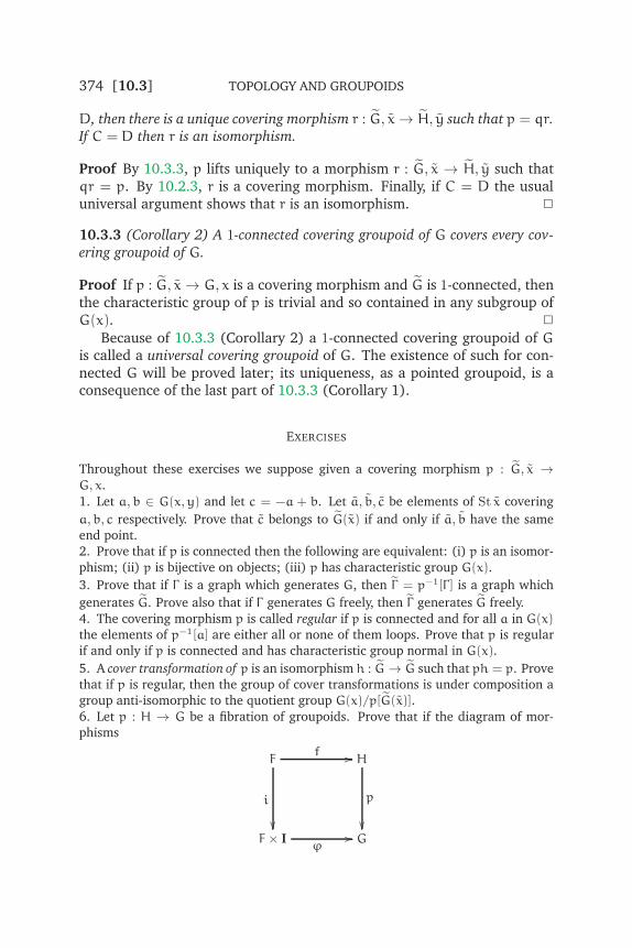
374 [10.3] TOPOLOGY AND GROUPOIDS
D, then there is a unique covering morphism r : G, x→ H, y such that p = qr.If C = D then r is an isomorphism.
Proof By 10.3.3, p lifts uniquely to a morphism r : G, x → H, y such thatqr = p. By 10.2.3, r is a covering morphism. Finally, if C = D the usualuniversal argument shows that r is an isomorphism. ✷
10.3.3 (Corollary 2) A 1-connected covering groupoid of G covers every cov-
ering groupoid of G.
Proof If p : G, x→ G, x is a covering morphism and G is 1-connected, thenthe characteristic group of p is trivial and so contained in any subgroup ofG(x). ✷
Because of 10.3.3 (Corollary 2) a 1-connected covering groupoid of Gis called a universal covering groupoid of G. The existence of such for con-nected G will be proved later; its uniqueness, as a pointed groupoid, is aconsequence of the last part of 10.3.3 (Corollary 1).
EXERCISES
Throughout these exercises we suppose given a covering morphism p : G, x →G, x.
1. Let a,b ∈ G(x,y) and let c = −a + b. Let a, b, c be elements of St x covering
a,b, c respectively. Prove that c belongs to G(x) if and only if a, b have the same
end point.
2. Prove that if p is connected then the following are equivalent: (i) p is an isomor-
phism; (ii) p is bijective on objects; (iii) p has characteristic group G(x).
3. Prove that if Γ is a graph which generates G, then Γ = p−1[Γ ] is a graph which
generates G. Prove also that if Γ generates G freely, then Γ generates G freely.
4. The covering morphism p is called regular if p is connected and for all a in G(x)
the elements of p−1[a] are either all or none of them loops. Prove that p is regular
if and only if p is connected and has characteristic group normal in G(x).
5. A cover transformation of p is an isomorphism h : G→ G such that ph = p. Prove
that if p is regular, then the group of cover transformations is under composition a
group anti-isomorphic to the quotient group G(x)/p[G(x)].
6. Let p : H → G be a fibration of groupoids. Prove that if the diagram of mor-
phisms
Ff //
i
��
H
p
��F× I
ϕ// G

COVERING SPACES, COVERING GROUPOIDS [10.4] 375
is commutative, where i is given by a 7→ (a, 0), then there is a morphism ψ : F×I→H such that ψi = f, pψ = ϕ. Prove further that if p is a covering morphism then
ψ is unique. [This is the covering homotopy property for fibrations and coverings of
groupoids; it would be possible, and indeed reasonable, to use this as the definition
of these terms.]
7. Let H and K be groupoids. The groupoid GPD(H,K) is defined to have objects
the morphisms H → K and morphisms from f to g the pairs (h, f) where h is a
homotopy f ≃ g. Make this construction explicit by defining the sum of homotopies
and verifying that this does give a groupoid. Prove that if H,K are groups, then
the object group of GPD(H,K) at the morphism f : H → K is isomorphic to the
centraliser of f[H] in K.
8. Prove that if also G is a groupoid, then there is a bijection
θ : Grpd(G×H,K)→ Grpd(G, GPD(H,K)).
[This is a lengthy exercise.]
9. Let p : K → L be a morphism of groupoids. Show how p induces through
composition a morphism p∗ : GPD(H,K)→ GPD(H,L) such that if p is a fibration,
then so also is p∗. Interpret the exact sequence of this fibration for specific cases.
10.4 Existence of covering groupoids
Our main purpose in this section is to prove that if x is an object of theconnected groupoid G, then any subgroup of G(x) is the characteristic gr-
oup of some covering morphism G, x → G, x. We shall deduce this from amore general construction of covering groupoids which is of considerableimportance even for the case G is a group.
LetG be a groupoid. An action ofG on a set consists of a set S, a functionw : S → Ob(G), and a partial function G × S S, (g, s) 7→ g · s, whichfor each x,y ∈ Ob(G), assigns to an element (g, s), where g ∈ G(x,y)and s ∈ w−1[x], an element g · s ∈ w−1[y]. The following rules are to besatisfied.
10.4.1 (i) If x ∈ Ob(G), s ∈ w−1[x], then 0x · s = s.(ii) If g ∈ G(x,y), h ∈ G(y, z), s ∈ w−1[x], then
(h+ g) · s = h · (g · s).
We also say G acts on S via w, and that S is a G-set.
EXAMPLE
1. Let p : G→ G be a covering morphism of groupoids, and let S = Ob(G),w = Ob(p). Then we obtain an action of G on S via w by assigning to s ∈ S

376 [10.4] TOPOLOGY AND GROUPOIDS
and g ∈ StG ps the target of the unique lift of g with source s. This actionis one of the essential features of 10.2.2.
It follows from the rules for an action that an element g ∈ G(x,y)
defines a bijection g || || : w−1[x] → w−1[y], s 7→ g · s. The action is said
to be transitive if for all x,y in Ob(G), s ∈ w−1[x], t ∈ w−1[y], there is ag ∈ G(x,y) such that g · s = t. In this case, all the sets w−1[x], x ∈ Ob(G),have the same cardinality.
If s ∈ w−1[x], the group of stability of s is the subgroup Gs of G ofelements g such that g · s = s. Such an element g is said to stabilise, or fix,s, and s is said to be a fixed point of g.
Given such an action, the semidirect product groupoid S ⋊ G is definedto be the groupoid with object set S and elements of (S⋊G)(s, t) the pairs(s,g) such that g ∈ G(ps,pt) and g · s = t. The addition in S⋊G is definedto be
(t,h) + (s,g) = (s,h+ g).
s
(s,g)
t = g · s
(t,h)
h · t
10.4.2 (a) The above construction makes S⋊G a groupoid.
(b) The projection p : S⋊G→ G, given on objects by w : S→ Ob(G) and on
elements by (s,g) 7→ g, is a covering morphism of groupoids.
(c) The groupoid S⋊G is connected if and only if the action is transitive.
(d) If s ∈ S, then the object group (S ⋊ G)(s) is mapped by p isomorphically
to Gs, the group of stability of s.
(e) The action ofG on S determined by the covering morphism p is the original
action.
Proof The proof of (a) is easy. Associativity is easily checked. The zero ats is (s, 0ps), and the negative of (s,g) is (g · s,−g).
It is clear from the definition that p is a morphism of groupoids. Also pis a covering morphism, because if g ∈ G(x,y), s ∈ w−1[x], then (s,g) isthe unique element of S⋊G which has source s and projects to g.
For (c), we need only note that (S⋊G)(s, t) is non-empty if and only ifthere is a g in G such that g · s = t.
For (d), (S⋊G)(s) consists of those (s,g) such that g · s = s, and so thisobject group is mapped by p to Gs.
Finally, (e) is clear. ✷
To use this result, we need a supply of actions of a groupoid. Here is away of obtaining a transitive action.

COVERING SPACES, COVERING GROUPOIDS [10.4] 377
10.4.3 Let x be an object of the connected groupoid G, and let C be a sub-group of the object group G(x). Let S be the set of (left) cosets
a+ C = {a+ c : c ∈ C}
for a in StG x. Let w : S → Ob(G) send a + C to the final point of a. Then
G acts transitively on S by g · (a + C) = g + a + C. The corresponding
connected covering morphism p : S⋊G, x→ G, x, where x is the coset C, has
characteristic group C. Further, p−1[x] is the set G(x)/C of left cosets of C in
G(x).
Proof Suppose a ∈ G(x,y), g ∈ G(y, z). Thenw(a+C) = y,w(g+a+C) =z. The rules 10.4.1(i) and (ii) are clearly satisfied. The action is transitive,because if a+C, b+C are cosets, and g = b− a, then g+ a+C = b+ C.It follows that S⋊G is connected.
The required characteristic group consists of the elements a of G suchthat the coset a+C is defined and is C, and this holds if and only if a ∈ C.Hence the characteristic group is C.
The final statement is obvious. ✷
The pointed groupoid constructed in 10.4.3 is sometimes in the litera-ture written Tr(G,C). It could also be written (G/C) ⋊ G. It is commonlycalled the covering groupoid of G based on the subgroup C of G(x). Theresults of the previous section show that a pointed, connected coveringmorphism is determined up to isomorphism by its characteristic group, sothe particular construction of Tr(G,C) is not always needed.
10.4.3 (Corollary 1) Any connected groupoid has a universal covering
groupoid.
Proof If G is a connected groupoid, and x ∈ Ob(G), then a universal cov-ering groupoid of G is Tr(G, 0x), where 0x is the trivial subgroup of G(x).Notice that in this case the set on which G acts is simply StG x, and theaction is via the target map τ : StG x→ Ob(G). ✷
The universal covering groupoid of G constructed in this corollary iscalled the universal covering groupoid of G based at x. Note that there is nounique universal covering groupoid of G, but only a family StG x ⋊ G ofthem indexed by the objects of G.
10.4.3 (Corollary 2) A connected covering morphism G, x→ G, x is an n-fold
covering if and only if its characteristic group has index n in G(x).
Proof By 10.3.3 (Corollary 1) G is isomorphic to Tr(G,C) where C is the
characteristic group of G, x. ✷

378 [10.4] TOPOLOGY AND GROUPOIDS
Here is a nice application of the idea of an action of a groupoid ona set. Let H be a groupoid, and let N be a totally disconnected normalsubgroupoid of H. Then we can form the quotient groupoid H/N (section8.3), which has the same objects as H, but the elements of (H/N)(x,y)are the cosets h + N(x), or, equally, N(y) + h, for all h ∈ H(x,y). It isconvenient to write such a coset as h + N, or N + h. There is a quotient
morphism p : H→ H/N sending an element h to the coset h+N. Note thatthe star of H/N at x consists of the cosets h+N(x) for all h in StH x.
Now we give an action of the groupoid H × H on the set H/N via thefunction w : H/N → Ob(H) × Ob(H) which sends an element h + N ∈(H/N)(x,y) to the pair (x,y). If a ∈ H(x,u), b ∈ H(y, v), and h + N ∈(H/N)(x,y), then we define
(a,b) · (h+N) = b + h− a+N ∈ (H/N)(u, v).
This can be conveniently represented by the diagram
xa //
h+N
��
u
b + h− a+N
��y
b// v.
The rules for an operation are easy to verify, using the normality of N,which gives h+N = N+ h for all h in H. Hence if h+N = k +N then
b+ h− a+N = b + h+N − a
= b + k +N− a
= b + k − a+N
so that the operation is well defined. Clearly (0x, 0y) · (h +N) = h +N. Iffurther c ∈ H(u,w), d ∈ H(v, z), then
(c,d) · (b + h− a+N) = d + b+ h− a− c+N
= (c+ a,d+ b) · (h+N),
as required.
Let (x,y) be an object ofH×H. Then the group of stability of the actionat (x,y) consists of pairs (a,b) ∈ H(x)×H(y) such that b+h−a+N = h+N,or, equivalently,
b + h+N = h+ a+N.

COVERING SPACES, COVERING GROUPOIDS [10.4] 379
Let �NH be the semidirect product groupoid (H/N) ⋊ (H × H). Then theobject group of �NH at the object (x, x) consists of pairs (a,b) such thata,b ∈ H(x) and a +N(x) = b +N(x). Thus (�NH)(x, x) is isomorphic tothe semidirect product group N(x)⋊H(x), which consists of pairs (n,a) ∈N(x)×H(x) with addition
(n,a) + (n ′,a ′) = (−a ′ + n + a ′ + n ′,a+ a ′)
the isomorphism being given by
(a,b) 7→ (−b + a,b).
A special case of this construction is when N is trivial, i.e. consistsonly of the zeros of H. Then we write 0 for N, and find that (�0H)(x) isisomorphic to H(x).
Going back to the general case, let ψ be the composite
�NH→ H×H→ H
of the covering morphism and the first projection. If x is an object of H,then the groupoid ψ−1[0x] is precisely the covering groupoid Tr(H,N(x))of H determined by the subgroup N(x) of H(x). Thus the groupoid �NH
gives a global description of the union of all the covering groupoids ofH determined by the subgroups N(x) for all objects x of H. This globaldescription is, of course, restricted to the case of normal subgroups. Wewill study this case further under the term regular covering groupoids insection 10.6.
We will use these constructions in the next section to give a convenienttopology on the groupoid (πX)/N for a normal totally disconnected sub-groupoid of the fundamental groupoid πX, for suitable X.
Remark In the theory of groups it is embarrassing that a subgroup C of agroup G determines a quotient group G/C if C is normal in G, but in thegeneral case it seems to determine nothing. In fact the action of G on theset of cosets G/C is important, and this action is nicely represented in thetheory of groupoids by the covering morphism (G/C) ⋊ G → G. Thus ifwe regard a group as a groupoid, then a subgroup of a group determines astructure of the same type. More generally, actions of groups on sets playan important role in the applications of groups, for example in enumerationquestions such as determining the numbers of necklaces with given num-bers of beads of various colours, and in chemistry determining the numbersof isomers of a given type. Some problems involving group actions are con-veniently formulated in terms of the exact sequence of a covering discussedin the exercises.

380 [10.4] TOPOLOGY AND GROUPOIDS
EXERCISES
1. Let p : G→ G be a covering morphism of groupoids and let x ∈ Ob(G). Let S be
the set p−1[px]. Show that the exact sequence of a fibration specialises to the exact
sequence
0→ G(x)→ G(px)→ S→ π0G→ π0G,
where exactness is formulated in section 7.2 for a fibration of groupoids. Show how
in the case G is a group, this sequence includes the information given by Lagrange’s
theorem on the index of a subgroup.
2. Let G be a group acting on a set S and let H be a group acting on a set T . Let
θ : G → H be a morphism of groups, and let ϕ : S → T be a function. Assume
that for all g ∈ G and s ∈ S, ϕ(g · s) = (θg) · (ϕs). Show that the function
ψ : S⋊ G→ T ⋊H given by (s,g) 7→ (ϕs, θg) is a morphism of groupoids and that
ψ is a fibration if and only if θ is surjective.
3. Continuing the notation of Exercise 2, let K = Kerθ, let s ∈ S and let F =
ϕ−1[ϕs]. Show that if g ∈ K then g · F ⊆ F, and that ψ−1[ϕs] = F ⋊ K. Assume
now that θ is surjective. Show how the exact sequence of a fibration gives rise to
an exact sequence of groups and pointed sets
1→ Ks → Gs → Hϕs → F/K→ S/G→ T/H
and describe the exactness properties in detail. Interpret this exact sequence in the
case that T is a singleton.
4. Assume that θ : G → H is an epimorphism of groups and that K = Kerθ. Let
G,H and K act on themselves by conjugation. Prove that if s ∈ G then there is an
exact sequence
1→ CK(s)→ CG(s)→ H→ [K]→ [G]→ [H]
where CG(s), the centraliser of s in G, is the set of g ∈ G such that g + s = s + g,
and [G] is the set of conjugacy classes of G. [Exercises 2, 3, 4 are from [HK82].]
5. Let H be a groupoid with object set X. An admissible section of H is a function
u : X → H such that ux has source x for all x ∈ X and the function sending x to
τux, the target of ux, is a bijection X → X. Prove that the set Γ(H) of admissible
sections of H is a group under the product vu : x 7→ vτux+ux. Prove that Γ(H) acts
on X by u · x = τux. Let G be a group acting on X. Prove that there is a bijection
between the set of morphisms f : G → Γ(H) such that (fg) · x = g · x for all x ∈ X,
and the set of morphisms X ⋊ G → H which are the identity on X. [The group of
admissible sections has an old history in work of [Ehr80].]
6. Let p : Y → X be a function of sets X,Y and let H be a groupoid with object set
Y. Define a groupoid p!(H) with object set X and an action of p!(H) on Y via p as
follows. The elements from x to x ′ are the functions u : p−1[x]→ H such that u(y)
has source y and target in p−1[x ′] and y 7→ τu(y) is a bijection p−1[x] → p−1[x ′].
The addition is given by
v+ u : y 7→ v(τuy) + u(y).

COVERING SPACES, COVERING GROUPOIDS [10.5] 381
The action is u · y = τu(y). Generalise Exercise 5 to obtain, for G a groupoid on X
operating on Y via p, a bijection of morphisms f : G→ p!(H) which are the identity
on objects and satisfy f(g) · y = g · y, and morphisms f∗ : Y ⋊G→ H which are the
identity on objects. [Exercises 5 and 6 are in [Cha77].]
7. Prove that a subgroup C of a free group G is free, and that if G is of rank r and
C is of index n in G, then C is of rank nr−n+ 1. [Construct G = Tr(G,C) and use
Exercise 2 of Section 10.3 and 8.2.1(c).]
8. Let R be a ring and I a left ideal of R; then, considering I simply as a subgroup of
the abelian group R, we can form the groupoid Tr(R, I). What additional structure
can be put on this object by using the multiplication? [This is more of a research
project than an exercise! Are the algebroids of [Mit85] relevant?]
9. Let G be a groupoid and let Cov(G) be the category whose objects are covering
morphisms p : G → G and whose morphisms from p : G → G to p ′ : G ′ → G are
determined by p,p ′ and a morphism r : G → G ′ such that p ′r = p. Prove that
Cov(G) is equivalent to the category Fun(G,Set) [Exercise 6 of Section 6.6]. [If
p : G → G is a covering morphism, define a factor Lp : G → Set which on objects
sends x 7→ p−1[x], and if a ∈ G(x,y), x ∈ p−1[x], then Lp(a)(x) is to be the target
of the element a which starts at x and covers a.]
10.5 Lifted topologies
In this section we apply the previous results to prove the existence of liftingsof maps and the existence of covering spaces—that is, we prove topologicaltheorems corresponding to 10.3.3 and 10.4.1. However this correspon-
dence is not complete since the existence of a covering map X→ X impliesa local condition on X. (We recall that all spaces are, in any case, assumedlocally path-connected.)
We introduce some useful language. If f : H → G is a morphism ofgroupoids, and x ∈ Ob(G), then χf(x) denotes G(x) if f−1[x] is empty, andotherwise denotes the intersection of the characteristic groups of f at y forall y ∈ f−1[x]. Thus χf is a wide, totally disconnected subgroupoid of G.
The notion of characteristic group and of χf will be used for maps ofspaces. More precisely, if f : Y → X is a map, then the characteristic group
of f at y is simply the characteristic group of πf : πY → πX at y; and thisgroup is also called the characteristic group of f : Y,y → X, fy or even, byan abuse of language, the characteristic group of Y,y. Similarly, we writeχf for χπf, so that χf is a subgroupoid of πX.
Let X be a space and let χ be any wide subgroupoid of πX. A subset Uof X is called weakly χ-connected if for all x in U the characteristic groupat x of the inclusion U → X is contained in χ(x). Clearly, any subset of aweakly χ-connected set is again weakly χ-connected.
We say X itself is semi-locally χ-connected if each x in X has a weakly

382 [10.5] TOPOLOGY AND GROUPOIDS
χ-connected neighbourhood; if χ is simply connected, this is also expressedas: X is semi-locally simply-connected. Our first result shows the utility ofthese definitions.
10.5.1 Let p : X→ X be a covering map. Then X is semi-locally χp-connected.
Proof Let U be a canonical subset of X. If x ∈ U and x ∈ p−1[x] then
the inclusion i : U, x → X, x lifts to a map U, x → X, x. So the morphismπU, x → πX, x lifts, and it follows that the characteristic group of U, x iscontained in the characteristic group of p at x. This is true for all x inp−1[x] and so the characteristic group of U, x is contained in χp(x).
Thus any canonical subset of X is weakly χp-connected. By definition ofcovering map, any x in X has a canonical neighbourhood. ✷
The following corollary is immediate.
10.5.1 (Corollary 1) If X is path-connected and has a 1-connected covering
space, then X is semi-locally simply-connected.
It may be proved using the methods of chapter 9 that the Hawaiian ear-ring [cf. Fig. 9.2, p. 344] is not semi-locally simply-connected (the originbeing a ‘bad’ point) and so this space has no 1-connected covering space.
Suppose now that X is a space and
q : G→ πX
is a covering morphism of groupoids. Let X be semi-locally χq-connected,and let
X = Ob(G), p = Ob(q) : X→ X.
We shall use q to ‘lift’ the topology of X to a topology on X.Let U be the set of all open, path-connected, weakly χq-connected sub-
sets of X. If U is any element of U consider the diagram
G
q
��πU
i
>>⑤⑤
⑤⑤
⑤⑤
⑤
i// πX
where i is induced by inclusion. By 10.3.3, i lifts to a morphism i : πU→ G;
the set i[U] is a subset U of X which we call a lifting of U. The set of all such
liftings ofU for allU in U is written U. Since X is semi-locally χq-connected,
the set U covers X.

COVERING SPACES, COVERING GROUPOIDS [10.5] 383
We need a lemma about these liftings.
Let V be path-connected and g : V → X a map such that g[V ] is con-
tained in a set U of U. Let g ′ : πV → G be a lifting of πg : πV → πX, and
let U be a lifting of U.
10.5.2 If g = Ob(g ′), and g[V ] has one point in common with U, then
g[V ] ⊆ U.
Proof Let x = gv be an element of g[V ] ∩ U and let x = px = gv. Considerthe diagram
G, x
q
��πV , v
g ′
66❧❧❧❧❧❧❧❧❧❧❧❧❧❧❧❧❧❧❧❧❧❧❧❧❧❧
g ′′// πU, x
i
<<②②②②②②②②②②②②②②
i// πX, x
in which g ′′ is induced by the restriction of g and i is a lifting of the mor-phism i induced by inclusion. Both g ′ and ig ′′ are liftings of πg : πV , v →πX, x. But V is path-connected, and so g ′ = ig ′′ (by 10.3.3). It follows that
g[V ] ⊆ U. ✷
A corollary of 10.5.2 is that if two liftings of an element U of U havea point in common, then they coincide—that is, two liftings of U eithercoincide or are disjoint.
We now prove that U is a base for the open sets of a topology on X
[cf. 5.6.3]. Let U, V be respectively liftings of elements of U, V of U, and
suppose w ∈ U ∩ V. Let w = pw and let W be an open path-connected setsuch that w ∈ W ⊆ U ∩ V; then W is weakly χq-connected and so has a
lifting W such that w ∈ W. By 10.5.2, W is contained in both U and V and
hence W ⊆ U ∩ V .
This completes the proof that U is a base for the open sets of a topology
on X. This topology on X will be called the topology of X lifted by q orsimply the lifted topology.
Suppose now that X has this topology.
10.5.3 Let f : Z → X be a map. If πf : πZ → πX lifts to a morphism
f ′ : πZ→ G, then
f = Ob(f ′) : Z→ X
is continuous and is a lifting of f : Z→ X. All liftings of f arise in this way.

384 [10.5] TOPOLOGY AND GROUPOIDS
Proof Let z ∈ Z and let U be a lifting of a setU of U such that fz ∈ U. ThenU is a neighbourhood of fz and so there is an open neighbourhood V of z,which may be assumed path-connected, such that f[V ] ⊆ U. Let j : V → Z
be the inclusion. Then f ′π(j) is a lifting of π(fj). By 10.5.2, f[V ] ⊆ U. Thisproves continuity of f.
If f : Z→ X is any lifting of f, then πf lifts πf, and so all liftings arise inthe above way. ✷
On the other hand, the lifted topology is relevant to the case of a givencovering map.
10.5.4 Let p : X→ X be a covering map. The topology of X is that of X lifted
by πp : πX→ πX.
Proof LetU be a canonical subset of X. If U is a path-component of p−1[U],
then the inclusion U → X lifts to a map U → X with image U. It follows
that U is a lifting of U. Clearly, these liftings U for all canonical subsets U
of X form a base for the open sets of the given topology on X.
On the other hand, let U be the set of open, path-connected, weakly χp-connected subsets of X. We know that each canonical subset of X belongs
to U. Let U ∈ U, and let U be a lifting of U. Because each point of U
has a canonical neighbourhood contained in U, it is easy to prove that U is
open in X and is mapped by p homeomorphically on to U. Therefore U iscanonical. Hence the lifted topology coincides with the given topology. ✷
By combining 10.5.4 with 10.5.3 and the corollaries to 10.3.3 we obtainthe following results.
10.5.4 (Corollary 1) If p : X, x → X, x and q : Y, y → X, x are connectedcovering maps with characteristic groups C,D respectively, and if C ⊆ D,
then there is a unique map r : X, x → Y, y such that p = qr. Further, r is a
covering map, and is a homeomorphism if C = D.
10.5.4 (Corollary 2) A 1-connected covering space of X covers every covering
space of X.
Because of 10.5.4 (Corollary 2) a 1-connected covering space of X iscalled a universal covering space of X. It is a special case of the last part of10.5.4 (Corollary 1) that any two universal covering spaces of a connectedspace X are homeomorphic.
We now show that the lifted topology does give rise to a covering space.
Let q : G → πX be a covering morphism, let X = Ob(G), p = Ob(q).Suppose also that X is semi-locally χq-connected and that U is the set ofopen, path-connected, weakly χq-connected subsets of X.
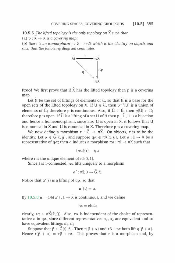
COVERING SPACES, COVERING GROUPOIDS [10.5] 385
10.5.5 The lifted topology is the only topology on X such that
(a) p : X→ X is a covering map;
(b) there is an isomorphism r : G → πX which is the identity on objects and
such that the following diagram commutes.
Gr //
q
❅❅❅
❅❅❅❅
❅❅❅❅
❅❅πX
πp
��πX
Proof We first prove that if X has the lifted topology then p is a coveringmap.
Let U be the set of liftings of elements of U, so that U is a base for theopen sets of the lifted topology on X. If U ∈ U, then p−1[U] is a union of
elements of U; therefore p is continuous. Also, if U ∈ U, then p[U] ∈ U;
therefore p is open. If U is a lifting of a setU of U then p | U,U is a bijection
and hence a homeomorphism; since also U is open in X, it follows that U
is canonical in X and U is canonical in X. Therefore p is a covering map.
We now define a morphism r : G → πX. On objects, r is to be the
identity. Let α ∈ G(x, y), and suppose qα ∈ πX(x,y). Let a : I → X be arepresentative of qα; then a induces a morphism πa : πI→ πX such that
(πa)(ı) = qα
where ı is the unique element of πI(0, 1).Since I is 1-connected, πa lifts uniquely to a morphism
a ′ : πI, 0→ G, x.
Notice that a ′(ı) is a lifting of qα, so that
a ′(ı) = α.
By 10.5.3 a = Ob(a ′) : I→ X is continuous, and we define
rα = cls a;
clearly, rα ∈ πX(x, y). Also, rα is independent of the choice of represen-tative a in qα, since different representatives a1,a2 are equivalent and sohave equivalent liftings a1, a2.
Suppose that β ∈ G(y, z). Then r(β+α) and rβ+ rα both lift q(β+α).Hence r(β + α) = rβ + rα. This proves that r is a morphism and, by

386 [10.5] TOPOLOGY AND GROUPOIDS
definition of r, (πp)r = q. By 10.2.3, r itself is a covering morphism. This
implies that for each x, y in X
r : G(x, y)→ πX(x, y)
is injective. It is also surjective, since any γ in πX(x, y) is covered by an
element γ of StGx; if γ ∈ G(x, y′) then ry = ry′ and so y = y′. Hence r
is an isomorphism. This proves that (a) and (b) are satisfied by the liftedtopology.
The uniqueness of a topology satisfying (a) and (b) follows from 10.5.4:since r is the identity on objects, the topology of X lifts by q and by πp to
the same topology on X. ✷
We now discuss covering spaces of cell complexes.
10.5.6 Let p : X → X be a finite covering map and let X be a cell complex.
Then X can be given a cell structure for which p is a cellular map.
Proof Let hα : Enα → X be a characteristic map for an nα-cell of X. By10.5.3, 10.5.4, and since Enα is 1-connected, hα lifts to a map hα : Enα →X. Since Enα is compact and X is Hausdorff, hα is a closed map; it is alsoinjective on Bnα (since hα is) and so hα maps Bnα homeomorphically to
a subset enα of X. That is, the open cells of X are liftings of the open cells
of X. By the uniqueness of liftings of maps, these cells of X are disjoint;
clearly they cover X.
It is clear that Xn = p−1[Xn]. It follows that for each lifting hα of hα,
we have hα[Sn−1] ⊆ Xn−1. The number of liftings of hα is finite. So the
maps hα are characteristic maps of a cell structure on X. The cellularity ofp is obvious. ✷
A similar result is true for any covering space of a cell complex. But if
the covering is infinite then the number of cells of X is infinite, and so itis necessary for this to discuss the topology of infinite cell complexes. Thegeneral topology useful for proving a covering space of a CW-complex is aCW-complex is given in [Mas67, p. 183–184].
We now give an entertaining application of these results on coveringspaces.
10.5.7 If n > 2 there is no map f : Sn → S1 such that f(−x) = −fx for all x
in Sn.

COVERING SPACES, COVERING GROUPOIDS [10.5] 387
Proof Suppose there is such an f and consider the diagram
Snf //
h
��
S1
k
��Pn(R)
g ′
==④④
④④
④④
④
g//❴❴❴❴❴ S1
in which h is the Hopf map and k is the map z 7→ z2. Both h, k are coveringmaps which identify antipodal points of the spheres they are defined on.
By the given condition on f, kf(−x) = kfx for all x in Sn. Therefore fdefines a map g : Pn(R) → S1 such that gh = kf. Since Pn(R), S1 havefundamental groups Z2, Z respectively, any characteristic group of g is 0.So g lifts to a map g ′ such that kg ′ = g. Notice that
kg ′h = gh = kf
so that g ′h and f are liftings of the same map. Hence g ′h and f agree at allpoints if they agree at one.
Let x ∈ Sn. Then the points g ′hx, fx are either the same or antipodalpoints. In the latter case, g ′h(−x) = g ′hx = −fx = f(−x). So g ′h, f agreeat either x or −x. Hence they agree everywhere, i.e., g ′h = f. But thisimplies that f(−x) = fx, and so we have a contradiction. ✷
10.5.7 (Corollary 1) Let n > 2 and let g : Sn → R2 be a map. Then there
exists a point x0 in Sn such that g(x0) = g(−x0).
Proof Let h : Sn → R2 be the map x 7→ g(x)−g(−x). Then h(−x) = −h(x)for all x in Sn.
Suppose there is no x0 in Sn such that g(x0) = g(−x0). Then h(x0) isnever zero, and so the map f : Sn → S1, x 7→ h(x)/‖h(x)‖, is well-defined.But then f(−x) = −f(x) for all x in Sn; this is impossible by 10.5.7. ✷
The above result with R2 replaced by Rn is known as the Borsuk-UlamTheorem. However, this more general theorem cannot be proved with themethods treated in this book.
Here is a nice application of the lifted topology.
10.5.8 Let X be a semi-locally simply connected space, and let N be a to-
tally disconnected normal subgroupoid of πX. Then the set of elements of the
quotient groupoid (πX)/N may be given a topology such that the projection
q = (σ, τ) : (πX)/N → X × X is a covering map and for x ∈ X the target

388 [10.5] TOPOLOGY AND GROUPOIDS
map τ : StπX x→ X is the covering map determined by the subgroup N(x) ofπ(X, x). Further there is a canonical isomorphism of groupoids
π((πX)/N) ∼= �NπX.
Hence the fundamental group of the space (πX)/N at x is isomorphic to the
semidirect product group N(x)⋊ π(X, x).
Proof Let H = πX. In section 10.4 we constructed a covering groupoid�NH of the product groupoid H × H such that �NH has object set H/N.We now use 10.5.5 to lift the topology of X to give a topology on the ob-ject set H/N of �NH. The formulae for the fundamental groupoid andfundamental group follow.
In order to identify the subspace St(πX)/N x of (πX)/Nwith the covering
space XN,x of X we have to examine in more detail the lifted topology on(πX)/N. This topology has a basis of sets (πV) + g + (πU) for g : x → y
in (πX)/N and U and V canonical neighbourhoods of x and y (where πUand πV also denote here their images in (πX)/N). The restriction of thistopology to St(πX)/N x has a basis of sets (πV) + g, for g ∈ St(πX)/N x. Sothe subspace topology is the lifted topology, as required. ✷
It is also true that (πX)/N is what we call a topological groupoid—thatis, all the structure maps of this groupoid are continuous for the given
topology. Thus all the covering spaces XN,x of X are nicely tied togetherin the one topological groupoid structure (πX)/N. However, we do notprove this here, but refer the reader to [BD75]. For more information ontopological groupoids, we refer the reader to [Mac05] and the referencesin [Bro87].
Finally for this section, we should mention an important fact about uni-versal covers of surfaces. Many readers will be familiar with the classifi-cation of compact, connected surfaces without boundary, as given in many
texts. The universal cover S of such a surface S is known to be either thesphere S2 or the plane R2. For a proof, see for example [Sti80]. The keypoint of the proof is to show that the universal cover of the orientable sur-face of genus two is R2.
EXERCISES
1. Prove that if q : X → X, r : Y → Y are covering maps, then so also is q × r :
X× Y → X× Y.
2. Let q : X→ πX be a covering morphism and let X be semi-locally χq-connected.
Let U be a set of open, path-connected weakly χq-connected subsets of X such that
U is a base for the open sets of X. Let U be the set of liftings of elements of U. Prove
that U is a base for the open sets of the lifted topology on X = Ob(G).

COVERING SPACES, COVERING GROUPOIDS [10.6] 389
3. Let r : Z → Y, q : Y → X be covering maps. Prove that qr : Z → X is a covering
map if and only if X is semi-locally Xqr-connected.
4. Prove that the Borsuk-Ulam Theorem does imply 10.5.7 (Corollary 1).
5. Prove that no subspace of R2 is homeomorphic to S2.
6. Let n > 2 and g : Sn → R2 be a map such that g(−x) = −g(x) for all x in Sn.
Prove that there is a point x0 in Sn such that g(x0) = 0.
10.6 The equivalence of categories
In this section we give a more sophisticated and comprehensive view of theprevious material by showing that there is a complete ‘translation system’from covering spaces to covering groupoids. The ‘translation system’ or dic-tionary is given by an equivalence of categories. This itself is illustrative of amodern trend in mathematics. Very often an equivalence of categories canhold a lot of information, giving two different views of what is essentiallythe same kinds of objects. Each view can be more appropriate and use-ful in some circumstances than the other. The interplay can then be quitepowerful. In our particular case, the equivalence between covering spacesof X and covering groupoids of πX gives a complete translation betweentopology and algebra, and in an elegant form. This translation is importantbecause of the wide occurrence of covering spaces in mathematics. For asurvey of this, see [Mag76] and [DD77, DD79].
We now define the categories we wish to prove equivalent. First we givethe topological example.
Let X be a Hausdorff, locally connected space. The category CovTop(X)
of covering spaces of X has objects the covering maps p : Y → X and hasas arrows or morphisms the commutative diagrams of maps, where p andq are covering maps,
Yf //
p
��❅❅❅
❅❅❅❅
❅❅❅❅
❅ Z
q
��⑦⑦⑦⑦⑦⑦⑦⑦⑦⑦⑦⑦
X.
It is convenient to write such a diagram as a triple (f,p,q). The compositionin CovTop(X) is then given by (g,q, r)(f,p,q) = (gf,p, r). Note that wemake no assumption that X, Y or Z are connected. By 10.2.4, f also is acovering map.
Let G be a groupoid. The category CovGrp(G) of covering morphismsof G has objects the covering morphisms p : H → G and has as arrows or

390 [10.6] TOPOLOGY AND GROUPOIDS
morphisms the commutative diagrams of morphisms, where p and q arecovering morphisms,
Hf //
p
❅❅❅
❅❅❅❅
❅❅❅❅
❅❅K
q
��⑦⑦⑦⑦⑦⑦⑦⑦⑦⑦⑦⑦⑦
G.
Again it is convenient to write such a diagram as a triple (f,p,q), and thecomposition is as in the topological case. By 10.2.3, f also is a coveringmorphism.
Now we come to our main result.
10.6.1 If X is a Hausdorff, locally connected and semi-locally 1-connected
space, then the fundamental groupoid functor π induces an equivalence of
categories
π! : CovTop(X)→ CovGrp(πX).
Proof If p : Y → X is a covering map of spaces, then π(p) : πY → πX is acovering morphism of groupoids, by 10.2.1. Since π is a functor, we alsoobtain the functor π!.
To prove π! an equivalence of categories, we construct a functor ρ :
CovGrp(πX)→ CovTop(X) and prove that there are homotopies of functors1 ≃ ρπ!, 1 ≃ π!ρ. The technical work for this has already been done, and itis simply a matter of assembling the facts.
Let q : G → πX be a covering morphism of groupoids. We suppose
the space X is given. Let X = Ob(G), and let p = Ob(q) : X → X. By
10.5.5, there is a topology on X making p a covering map, and there is
an isomorphism r : G → πX. We have to prove that this topology on X isnatural with respect to morphisms in the category CovGrp(πX), and that ralso is natural.
Let (f,q, s) be a morphism in CovGrp(πX), where f : G → H. Let U bethe set of all open, path-connected, subsets U of X such that the inclusionU → X maps the fundamental group of U trivially. In section 10.5 we
showed how to lift the cover U to give covers Uq, Us of X = Ob(G) and
Y = Ob(H) respectively. These covers are bases for the topologies of X and
Y respectively. Let x ∈ X, and suppose Us is an element of Us containing fx.
Then U = s[Us] belongs to U and U lifts to an element Uq of Uq containing

COVERING SPACES, COVERING GROUPOIDS [10.6] 391
x. Further f[Uq] = Us. So f : X → Y is continuous. This defines ρ onmorphisms, and it is clear that ρ is a functor.
The homotopy of functors r : 1 ≃ π!ρ is defined in essence in 10.5.5.The only extra fact which has to be proved is that r is natural. So let(f,q, s) be a morphism in CovGrp(πX) as above. We have to prove that thefollowing diagram is commutative:
Gr //
f
��
πX
π(Ob(f))
��H
r // πY.
This requires examining the definition of r. Let α be an element of G whichstarts at x. Let a : I→ X be a representative of qα ∈ πX. Then a induces amorphism πa : πI→ πX such that (πa)(ı) = qα. Further, πa lifts uniquely
to a morphism a ′ : πI, 0 → G, x. Then rα is the class of the path Ob(a ′) :
I → X. Let β = fα, and apply the same process to give b ′ : πI, 0 → H, fx,where b = Ob(f)a. Since b ′ is uniquely determined by b, it follows thatrf(α) = π(Ob(f))r(α).
Finally we have to construct a homotopy θ : 1 ≃ ρπ!. But X = Ob(πX)
and the topology of X is precisely the lifted topology. So in fact 1 = ρπ!. Sothe proof is complete. ✷
The significance of this result is that it shows that the functor π! allowsus to translate a topological problem on covering spaces to an algebraicproblem on covering groupoids. This is one of those rare examples of acomplete and faithful translation. Usually a functor ‘forgets’ some of theoriginal formulation. Such forgetting has the advantage of translating aproblem into a simpler one, and one possibly with more opportunities forcalculation, but it does mean that some of the original geometry is lost.
As one example of the use of this translation, we will study the auto-morphisms of an object of the category CovGrp(G). This gives the group of
covering isomorphisms of a covering morphism, and our results will then, byvirtue of the equivalence of categories, yield results on the automorphismsof an object of CovTop(X). But first we solve a more general problem forwhich we require some notation.
Let A be a group, and let F,C be subgroups of A. We define
MA(F,C) = {a ∈ A : F ⊆ a+ C− a}.
Let us temporarily write this set asM. In general it is not true that a,b ∈Mimplies a+b ∈M. However, this is true if F = C, in which case the addition

392 [10.6] TOPOLOGY AND GROUPOIDS
gives M the structure of a monoid (i.e. it satisfies the associativity and unitaxioms, but inverses need not exist); in general, M is not in this case agroup. To obtain a group in this case we consider the usual normaliser of Fin A, namely
NA(F) = {a ∈ A : F = a+ F− a}.
Then NA(F) is the largest subgroup of A in which F is a normal subgroup.
10.6.2 Let Z,G,H be connected groupoids, and let p : H → G be a covering
morphism. Let f : Z → G be a morphism of groupoids, and let L(f,p) be the
set of liftings of f to morphisms Z → H. Let z ∈ Ob(Z), x ∈ Ob(H) and
suppose px = fz. Let
A = G(px), F = f[Z(z)], C = p[H(x)].
Then there is a surjection ϕ from MA(F,C) to L(f,p) with the property that
ϕa = ϕb if and only if there is an element c ∈ C such that b = a+ c.
Proof Let M = MA(F,C) and let a ∈ M. Then a lifts uniquely to anelement a in StG x. Let y be the end point of a. By 10.3.2, the characteristicgroup of p at y is a + C − a. Since F ⊆ a + C − a, it follows from 10.3.3that f lifts uniquely to a morphism f such that f(z) = y. We set ϕ(a) = f.
a
y x
a
Fig. 10.2
If f : Z → H is any lifting of f, then since H is connected, there is anelement a in H(x, f(z)). If a = pa then ϕ(a) = f. This proves that ϕ issurjective.
Suppose now that a,b ∈ M, and that a, b are lifts of a,b starting at x.If b = a+ c where c ∈ C, then c has a lift c ∈ H(x) and then a+ c also liftsb, and has the same target as a. Hence ϕ(a) = ϕ(b). On the other hand, ifϕ(a) = ϕ(b) then a and b have the same target and so c = −a+ b is welldefined. Let c = p(c). Then b = a+ c. This proves the result. ✷
In the case f = p we can make the result a bit stronger. Recall thata covering isomorphism h : H → H of a covering morphism p : H → Gis an isomorphism of groupoids such that ph = p. Clearly the set of thesecovering isomorphisms forms under composition a group, and we write thisgroup as Aut(p).

COVERING SPACES, COVERING GROUPOIDS [10.6] 393
10.6.3 Let p : H → G be a covering morphism of connected groupoids, letx ∈ Ob(H) and let C = p[H(x)] be the characteristic group of p at x . Then
Aut(p) is anti-isomorphic to the quotient of the group NG(px)(C) by its nor-
mal subgroup C.
Proof Let A = G(px). Then N = NA(C) is the normaliser of C in A andC is normal in N so that the quotient group N/C is well defined. We knowthat if a,b ∈ N then ϕ(a),ϕ(b) are morphisms h, k : H→ H, say, such thatph = h, pk = k. We now prove that ϕ(b + a) = hk.
Let a, b ∈ StH x have final points y and u, and lift a,b respectively.Then h(x) = y, k(x) = u, and so h(u) = hk(x). Hence h(b) ∈ H(y,hk(x)).But h(b) + a is defined, belongs to StH x, and lifts b+ a. Since phk = p, itfollows that ϕ(b + a) = hk.
Since ϕ(0) is the identity H→ H, and ϕ is an anti-morphism, it followsthat h = ϕ(a) is an isomorphism. The result follows. ✷
The next result is useful when combined with the previous one. First,we say that an element g of a groupoid G is a loop if it belongs to somevertex group of G, i.e. if g has the same source and target. As motivationfor the result, consider the following picture of two graphs whose labellingsshow how they cover the space X = S1 ∨ S1 consisting of a wedge of twocircles labelled a and b.
a
b
a
b
a
b
a
b
a
b
a
b
Fig. 10.3
In the first example, the edges with a given label are either all or none ofthem loops. In the second example, the edges labelled a consist of one loopand two non loops.
10.6.4 Let p : H → G be a covering morphism of groupoids. Consider the
following conditions:
(a) for all loops a in G, either all or no lifts of a are loops;
(b) for all objects x of H, the characteristic group p[H(x)] is normal in G(px).
Then (a)⇒ (b), and if H is connected, (b)⇒ (a).
Proof (a) ⇒ (b) Let x be an object of H and let C = p[H(x)]. Let c ∈ C,a ∈ G(px). We need to prove that −a + c + a ∈ C. Let b ∈ H(x,y) lift a.

394 [10.6] TOPOLOGY AND GROUPOIDS
By (a), c lifts to an element d of H(y). Then −b + d + b belongs to H(x)and is mapped by p to −a+ c+ a. Hence −a+ c+ a ∈ C.
d
y
b
x p
a
c
Fig. 10.4
(b) ⇒ (a) Let x,y be objects of H such that p(x) = p(y), and let c ∈C = p[H(x)]. Since H is connected, there is an element b in H(x,y). Leta = p(b). Now −a + c + a ∈ C, since C is normal in G(px), and so−a+ c+ a = p(e) where e ∈ H(x). Then
p(b+ e− b) = a− a+ c+ a− a = c.
But b+ e− b belongs to H(y) and is a loop. So c lifts also to a loop at y. ✷A covering morphism p : H → G of groupoids is called regular if H and
G are connected and one of the conditions (a) or (b) of the previous resultis satisfied.
10.6.4 (Corollary 1) If p : H→ G is a regular covering morphism of groupoids,
and C is a characteristic group of p at an object x of H, then the group of cov-
ering isomorphisms of p is anti-isomorphic to the quotient group H(x)/C.
Proof This is immediate from 10.6.3 and 10.6.4. ✷
We can now use the equivalence of categories to translate these ideasand results to the topological case. Let p : Y → X be a covering map. If aspace Z, and also Y and X, are path connected, then the set of lifts of a mapf : Z→ X to a map Z→ Y can be entirely determined from 10.6.2, by con-sidering the corresponding problem for the fundamental groupoids. Also,p is called regular if the corresponding covering morphism of groupoidsπp : πY → πX is a regular covering morphism. So we immediately obtain:
10.6.4 (Corollary 2) Let p : Y → X be a regular covering map of spaces. Let
y ∈ Y. Then the group Aut(p), of homeomorphisms h : Y → Y such that
ph = p, is anti-isomorphic to the quotient group of the fundamental group
π(X,py) by the normal subgroup p∗[π(Y,y)]. In particular, if X is connected
and Y is a universal cover of X, then the group of homeomorphisms h : Y → Y
such that ph = p is anti-isomorphic to the fundamental group π(X, x) at any
point x in X. ✷
The importance of this last result is that the fundamental group is shown

COVERING SPACES, COVERING GROUPOIDS [10.7] 395
to occur as a group of automorphisms. This links two basic motivating ex-amples for group theory, namely symmetry groups and fundamental groups.This link has proved useful in a number of areas of mathematics. There iseven a proof of the Van Kampen theorem for the fundamental group en-tirely in terms of covering spaces, see for example [DD77, DD79]. Howevera proof of theorem 6.7.2 in this spirit is not available in the literature.
There is also a notion of symmetry groupoid, whose applications to dif-ferential geometry and topology were initiated by [Ehr80]. For furtherreferences on this, see [Mac05] and the survey article [Bro73].
EXERCISES
1. Prove that a connected 2-fold covering morphism is regular.
2. We say two covering spaces Y,Z of X = S1∨S1 are equivalent if Y is homeomor-
phic to Z. Find representatives of all equivalence classes of 3-fold covering spaces of
X. Which of these are regular? For each connected 3-fold covering, use the method
of proof of the Nielsen–Schreier theorem (see 10.8.2) to give a subgroup H of the
fundamental group F of X at the base point, such that H determines the covering.
In the regular cases, write down the quotient group F/H.
3. Carry out a similar exercise to the previous one but for 4-fold covering spaces of
S1 ∨ S1.
4. Illustrate the application of 10.6.2 and 10.6.3 by explicit examples for the case
G and Z are groups.
5. With reference to the paragraph before 10.6.2, give an example where a,b ∈Mbut a + b /∈M. Also, give an example of a group G, subgroup H of G and element
g ∈ G such that g+H− g is a proper subset of H. [An example of this type is given
in [Ros78, p. 62].]
6. Construct regular and non-regular but connected 3-fold coverings of the graphs
shown in Fig. 10.5:
Fig. 10.5
10.7 Induced coverings and pullbacks
In this section we deal with the important topics of restricting coverings tosubspaces, and pulling back coverings.
We have already defined pushouts in any category. The dual notion ofpullback arose earlier than pushout, in the theory of fibre spaces, and in fact

396 [10.7] TOPOLOGY AND GROUPOIDS
suggested the term pushout for the dual term. We have defined pullbacksin a general category in an exercise in chapter 6. Here we take a moreconcrete approach.
Suppose given two maps f : A → X and p : Y → X. The pullback of fand p, also called the fibre product, is the subspace P of A× Y given by
P = A f×p Y = {(a,y) ∈ A× Y : fa = py}.
It is common to write also P = A ×X Y, since we can think of A and Y asspaces over X.
There is a diagram
Pf //
p
��
Y
p
��A
f // X
(10.7.1)
in which p : (a,y) 7→ a, f : (a,y) 7→ y. Then the diagram (10.7.1) iscommutative: pf = fp. It is also a pullback in the following sense: givenany commutative diagram
P ′ f ′ //
p ′
��
Y
p
��A
f // X
there is a unique map r : P ′ → P such that fr = f ′, pr = p ′. Here r is simplythe restriction of the map (p ′, f ′).
If f is injective then the point (a,y) of P is determined entirely by theelement y ∈ p−1f[A]. If further f is an embedding, then the map P →p−1f[A], (a,y) 7→ y, is a homeomorphism with inverse y 7→ (f−1p(y),y).This makes the important point that if f is the inclusion of a subspace A ofX, then we may identify A×X Y with p−1[A].
10.7.2 If p : Y → X is a covering map, then for any map f : A → X, the
induced map p : A ×XY → A is also a covering map. Further, if p is an n-fold
covering map, so also is p.
Proof We prove that if U is a canonical open set in X, then f−1[U] is acanonical open set in A. Suppose then that ϕ : p−1[U] → U × F is a

COVERING SPACES, COVERING GROUPOIDS [10.7] 397
homeomorphism of the form y 7→ (py,ϕ2y), with inverse ψ, where F is adiscrete space. Then we may define maps
ϕ′ : p−1f−1[U]→ f−1[U]× F, ψ ′ : f−1[U]× F→ p−1f−1[U],
(a,y) 7→ (a,ϕ2y), (a, z) 7→ (a,ψ(fa, z))
and check that
ψ ′ϕ′(a,y) = ψ ′(a,ϕ2y) = (a,ψ(fa,ϕ2y))
= (a,ψ(py,ϕ2y)) = (a,ψϕy) = (a,y),
ϕ′ψ ′(a, z) = ϕ′(a,ψ(fa, z)) = (a,ϕ2ψ(fa, z)) = (a, z).
This proves that p is a covering map and also the statement about n-coverings. ✷
There are similar notions of pullback for groupoids. Let f : L → G andp : H→ G be groupoid morphisms. The pullback square defined by f and pis the diagram
Qf //
p
��
H
p
��L
f // G
(10.7.3)
in which Q is the subgroupoid of the product groupoid L×H of pairs (l,h)(of elements or objects) such that fl = ph. The groupoid Q is also calledthe fibre product of L and H over G, and is written L×GH. The morphismsf and p are given respectively by (l,h) 7→ l, (l,h) 7→ h. We shall also needthe fact that:
10.7.4 If f : L → G and p : H → G are morphisms of groupoids, and p is a
covering morphism, then p : L×G H→ L is also a covering morphism.
Proof This is a straightforward check. Let Q = L ×G H and let (x,y) ∈Ob(Q). Then fx = py. We have to prove that p : StQ(x,y) → StL x isbijective. Let l ∈ StL x. Since p is a covering morphism, and fx = py,there is an element h ∈ StH y such that fl = ph. Clearly p(l,h) = l, and(l,h) ∈ StQ(x,y). Also (l,h) is the only such element, since p is a coveringmorphism. ✷
One special case of the pullback construction is important. Let p : H→G be a morphism and let f : L → G be the inclusion of the subgroupoid Lof G. Then the element (l,h) of L×G H can be identified with the element

398 [10.7] TOPOLOGY AND GROUPOIDS
h, subject to the sole condition that ph ∈ L. Hence we can identify L×G Hand p−1[L].
As may be expected, it is of interest to compare pullbacks of spaces andpullbacks of the corresponding fundamental groupoids.
10.7.5 Suppose given a pullback (10.7.1) of spaces. Then there is an induced
morphism of groupoids
θ : π(A×X Y)→ πA×πX πY
which is the identity on objects. Further, if p is a covering map of spaces, then
θ is an isomorphism.
Proof The morphism θ is determined by the morphisms π(p), π(f), and theproperties of the pullback of groupoids. Clearly θ is the identity on objects.
Consider the diagram
πPθ //
πp
$$❍❍❍
❍❍❍❍
❍❍❍❍
❍❍❍❍
πA×πX πY
(πp)
��πA.
We know that πp and (πp) are covering morphisms. It follows that θ isa covering morphism. But θ is the identity on objects. Therefore θ is anisomorphism. ✷
Suppose then that (10.7.1) is a pullback of spaces and that p is a cov-ering morphism. Our aim is to find information on πP. By the last result,it is sufficient to prove a result about pullbacks of covering morphisms ofgroupoids. The result we want is conveniently expressed in terms of anexact sequence.
10.7.6 Suppose that (10.7.3) is a pullback of groupoids and that p is a cov-ering morphism. Let (l,y) ∈ Ob(Q), so that fl = py = x, say. Then there is
a sequence
Q(l,y)i−→ L(l) ×H(y) δ−→ G(x)
∆−→ π0Qq−→ π0L×π0G π0H
in which
(1) i is the inclusion;
(2) L(l)×H(y) acts on the set G(x) by (λ, η) · γ = fλ + γ− pη, and ∂ is the
function (λ, η) 7→ fλ− pη;

COVERING SPACES, COVERING GROUPOIDS [10.7] 399
(3) ∆γ = cls(l, z) where z is the end point of the lift γ of γ with initial pointy;
(4) q : cls(b, z) 7→ (clsb, cls z).
This sequence is exact in the sense that:
(a) i is a monomorphism and ∂(λ, η) = ∂(µ, ξ) if and only if (−λ + µ,−η +
ξ) ∈ Q;
(b) ∆γ = ∆δ if and only if there are elements λ ∈ L(l), η ∈ H(y) such that
δ = fλ + γ− pη;
(c) Im∆ = q−1(cls l, clsy);(d) q is surjective.
Proof The functions in the sequence are well defined so that it only re-mains to verify exactness.(a) The morphism i is an inclusion and so a monomorphism. By definitionof ∂, we have ∂(λ, η) = ∂(µ, ξ) if and only if fλ − pη = fµ − pξ. This isequivalent to f(−λ + µ) = p(−η + ξ), which is itself equivalent to (−λ +µ,−η+ ξ) ∈ Q.(b) Suppose δ = fλ + γ − pη as given. If γ ∈ H(y, z) covers γ, then γ − η
covers γ − pη and has initial point y, so that z = ∆γ = ∆(γ − pη). If
λ ∈ H(z,w) covers fλ, then (λ, λ) joins (l, z) to (l,w) in Q, and so ∆(γ −
pη) = ∆(fλ+ γ− pη).Suppose conversely that ∆γ = ∆δ. Let γ ∈ H(y, z) cover γ and let
δ ∈ H(y,w) cover δ. Since (l, z), (l,w) lie in the same component of Q,there are elements λ ∈ L(l, l), κ ∈ H(z,w) such that fλ = pκ. Let η =
−δ+ κ + γ ∈ H(y). Then
fλ = pκ = pδ+ pη− pγ = δ+ pη− γ
which gives δ as required.(c) Note that if γ ∈ H(y, z) covers γ ∈ G(x), then
q∆(γ) = (cls l, cls z) = (cls l, clsy).
Suppose conversely that q(cls(b,w)) = (cls l, clsy). Then fb = pw andthere are elements λ ∈ L(l,b), κ ∈ H(y,w). Let η ∈ H(z,w) lift fλ, and letγ = −fλ + pη. Then γ ∈ G(x) and −η + κ belongs to H(y, z) and lifts γ.Hence ∆(γ) = cls(l, z). But cls(l, z) = cls(b,w) since (λ, η) : (l, z) → (b,w)
in Q.(d) Finally we prove that q is surjective. Let clsb ∈ π0L, clsw ∈ π0H besuch that cls fb = clspw in π0G. Then there is an element κ : pw → fb
in G. Let η : w → z lift κ. Then (b, z) is an object of Q and q(cls(b, z)) =(clsb, cls z) = (clsb, clsw). ✷
10.7.6 (Corollary 1) If L and H are connected groupoids, then there is a

400 [10.7] TOPOLOGY AND GROUPOIDS
bijection from π0Q to the set of distinct double cosets
f[L(l)]γp[H(y)]
for γ ∈ G(x).
Proof This just says that the orbits of the action of L(l)×H(y) on G(x) arethese double cosets. ✷
10.7.6 (Corollary 2) Suppose that L and H are connected groupoids and that
H is simply connected, so that p : H → G is a universal covering morphism.
Then the pullback Q = L ×G H is connected if and only if f : L(l) → G(x) is
surjective; andQ is simply connected if and only if f : L(l)→ G(x) is injective.
Proof Since H is 1-connected and L is connected, the exact sequence of10.7.6 becomes
1→ Q(l,y)→ L(l)→ G(x)→ π0Q→ 1,
from which the statements follow immediately. ✷
These results on pullbacks of covering morphisms of groupoids have,by 10.7.5, immediate applications to pullbacks of covering maps of spaces.We leave the reader to make the obvious conclusions.
We refer the reader to the exercises for a different treatment of theexact sequence in 10.7.6; it is deduced from the sequence for a coveringof groupoids by using the notion of homotopy pullback. This treatmentis more elegant but would have taken us too far afield. The advantageof the use of homotopy pullbacks is that one obtains exact sequences forany pair of morphisms of groupoids L → G, H → G, and in particularthere are exact sequences for the case L,G,H are groups. It is shown in[BHK83] how the exact sequence of 10.7.6 can be used in conjunction withnon-abelian cohomology with coefficients in a groupoid to deduce the VanKampen theorem for the fundamental groupoid.
EXERCISES
1. [Exercises 1–5 are taken from [BHK84].] Let f : L → G and p : H → G be
morphisms of groupoids. The homotopy pullback Z = Z(f,p) is defined as follows.
The objects of Z are to consist of all triples (l,γ, y) where l ∈ Ob(L), y ∈ Ob(H),
and γ : fl → py in G. An element of Z((l,γ, y), (l ′,γ ′,y ′)) is a triple (γ, λ, η)
such that λ ∈ L(l, l ′), η ∈ H(y,y ′) and pη + γ = γ ′ + fλ. Define r : Z → L × H by
(l,γ,y) 7→ (l,y) on objects, (γ, λ, η) 7→ (λ, η) on elements. Prove that r is a covering
morphism and that the induced function π0Z→ π0L×π0Gπ0H is surjective. Explain
how Z derives from an action of the groupoid L×H.

COVERING SPACES, COVERING GROUPOIDS [10.8] 401
2. Continuing the notation of Exercise 1, let Q = L×G H be the pullback of f and
p. Define ϕ : Q→ Z by (l,y) 7→ (l, 1fl,y) on objects, (λ, η) 7→ (1, λ, η) on elements.
Prove thatϕ is full and faithful and that the induced morphism π0ϕ : π0Q→ π0Z is
injective. Prove that π0ϕ is surjective, and hence that ϕ is a homotopy equivalence,
if and only if for each object (l, γ,y) of Z there are elements λ : l → l ′ in L,
η : y ′ → y in H such that fl ′ = py ′ and γ = pη+ fλ. Use this result, Exercise 1, and
the exact sequence of a fibration to deduce 10.7.6.
3. Let G be a group and let L and H be subgroups of G. For γ ∈ G let κγ :
H ∩ γ−1Lγ → L × H send η 7→ (γηγ−1,η). By considering the exact sequence at
the base point (1,γ, 1) of the homotopy pullback of the inclusions L → G, H → G,
prove that G is bijective with the disjoint union of the cosets (L × H)/ Imκγ for γ
in a set of representatives of the double cosets LγH. Hence show that if G is finite
and |G| denotes the order of G then
|G| = |L||H|(Σγ|H ∩ γ−1Lγ|−1).
4. Let L and H be subgroups of the group G such that G = LH. Let γ ∈ L∩H. Prove
that there is an exact sequence
1→ CL∩H(γ)→ CL(γ) ×CH(γ)→ CG(γ)→ [L ∩H]→ [L]×[G] [H]→ 1
where CG(γ) is the centraliser of γ in G and [G] is the set of conjugacy classes of G.
[Let the given groups act on their underlying sets by conjugation and consider the
induced morphisms of groupoids L⋊ L→ G⋊G← H⋊H.]
5. Let f : L → G be a morphism of groupoids and let Pf = Z(f, 1G). Define i :
L → Pf by l 7→ (l, 1fl, fl) on objects and λ 7→ (λ, fλ) on elements. Prove that i is a
homotopy equivalence. Define p : Pf → G by (l,γ,y) 7→ y on objects and (λ, η) 7→ η
on elements. Prove that pi = f and that p is a fibration of groupoids. Interpret the
exact sequence of the fibration p in the case f is the inclusion of a subgroup of the
group G.
6. Let Set· be the category of pointed sets: thus an object of Set· is a pair (X, x)
where x ∈ X, and a morphism (X, x) → (Y,y) is a pair (f, x) where f : X → Y is a
function and f(x) = y. Let p : Set· → Set be the ‘forgetful’ functor which on objects
sends (X, x) 7→ X and on morphisms sends (f, x) 7→ f . Prove that p is a covering
morphism. Let q : G→ G be any covering morphism of groupoids. Prove that there
is a functor q ′ : G→ Set and an isomorphism r : G→ G×Set Set· such that pr = q.
10.8 Applications to subgroup theorems in
group theory
We give some other applications of covering spaces to what are called sub-
group theorems. The general problem is the following. Let H be a subgroup
of the group G and suppose that information on G is given: deduce useful
information on H. The classical result of this type is that a subgroup of afree group is also a free group.

402 [10.8] TOPOLOGY AND GROUPOIDS
Covering morphisms give a method for dealing with this kind of prob-lem. For if H is a subgroup of the group G, then H is a vertex group of the
covering morphism p : G → G determined by H. If the information on G
can be lifted to information on G, then the problem may be changed intoone of obtaining information on a vertex group of a groupoid from infor-mation on the groupoid itself. Before going ahead with the theory, we workout a specific example.
For the rest of this section we use multiplicative notation for the com-position in groups and in groupoids.
EXAMPLE
1. Let F be the free group on the two elements x and y. Let H be thenormal subgroup of F generated by the elements x3, y2, and xyxy. Thequotient group F/H is well known to be the permutation group S3 on the set{1, 2, 3}, where x represents the cyclic permutation (123) and y representsthe transposition (23). Thus H is the kernel of the quotient morphism q :
F → S3. The directed graph X = {x,y} which generates F can be picturedas the wedge of two circles. Fig. 10.6(i) (do not pay attention to the dotsfor the moment) is a picture of what is called the Cayley graph of the groupS3 for the generators x,y. What it shows is how the generators act on theelements of the group. So an arrow labelled x is an arrow w → xw, and
an arrow labelled y is an arrow w→ yw, for w ∈ S3. We call this graph X.
Then X = p−1[X] where p : F→ F is the covering morphism determined by
the subgroup H of F, so that F = S3 ⋊ F, where S3 is here taken as a set onwhich F acts.
(i)
1 x
yx
y
y y
x xx x
y y
(ii)
Fig. 10.6
We shall prove below that F is the free groupoid on the graph X. Hencewe can use the methods of section 8.2 to obtain a basis for the vertex group
F(1) of F, a vertex group which is isomorphic to H. We choose a maximal
tree T in X, for example that given by Fig. 10.6(ii). This tree determines a
retraction r : F → F(1), where we may identify F(1) and H, and the basis

COVERING SPACES, COVERING GROUPOIDS [10.8] 403
for H consists of the elements of r[∆] where ∆ consists of the edges of X notin T . In this instance the basis for H is then given by the seven elements
yy, y−1xyx, x−1yx−1y, xxx, y−1xxxy, xyxy, y−1x−1yx−1
where in the above the elements which come from ∆ are written in boldtype.
Another interesting feature which can be drawn from Fig. 10.6(i) is thatof an identity among relations. Write r = x3, s = y2, t = xyxy. These areelements of the free group F. The following wordw in F, in which vu meansu−1vu,
w = t(s−1)xyty−1xy(r−1)ys−1(s−1)x
−1y−1
tx
represents a path in X which starts from the base point 1, then goes out toa base point, as represented by a dot, of a 2-cell of our planar diagram of
X, goes once round the 2-cell, and then returns to the base point 1, beforetraversing another such path, till each 2-cell has been traversed once. Adirect check shows that w = r, so that wr−1 = 1 in F. This word wr−1
in r, s, t and their inverses and conjugates is called an identity among the
relations for the presentation 〈x,y : r, s, t〉 of the group S3. These ideas arethe start of a 2-dimensional theory corresponding to that of free groups andfundamental groupoids. For more information, see [BH82] and [Bro70].
Now we return to subgroup theorems. The key result for our purposesis the following, which links the methods of universal groupoids of chapter8 with those of covering morphisms. We use the notion of pullback fromthe last section.
10.8.1 Let f : L → G be a universal groupoid morphism, and let p : G → G
be a covering morphism. Consider the pullback diagram
L×G Gf //
p
��
G
p
��L
f // G.
Then f is universal.
Proof We use the description of universal groupoid morphisms given in
section 8.1. Let h be a non-identity element of G. We prove that h hasa unique representation as a product h = (fqn) · · · (fq1) where the qi are

404 [10.8] TOPOLOGY AND GROUPOIDS
non-identities in Q = L ×G G and no product qi+1qi exists in Q. Letg = ph. Since f is universal, and ph is not an identity ofG, there is a uniquerepresentation ph = (fln) · · · (fl1) where the li are non-identities in L andno product li+1li exists in L. Hence we can uniquely write h = hn · · ·h1
where phi = fli. Setting qi = (li,hi) gives the required representation.
We still have to prove this representation is unique. Suppose also h =
(fq′m) · · · (fq′
1), where the q′i satisfy conditions similar to those for the qi.
Since p is a covering morphism, the pq′i are not identities in L. Also the
product (fq′i+1)(fq
′i) exists in H, and therefore the product (pq′
i+1)(pq′i)
does not exist in L. Therefore m = n and pq′i = li, since f is universal. It
now follows that q′i = qi for all i. Hence f is universal. ✷
10.8.1 (Corollary 1) Let p : H→ G be a covering morphism and suppose that
G is the free groupoid on a graph X. Then H is the free groupoid on the graph
p−1[X].
Proof Let ϕ : D(X) → X be the dispersion of the graph X (see section8.2). According to 8.2.1(a), the induced morphism ϕ : F(D(X)) → G isstrictly universal. Let Q be the pullback F(D(X)) ×G H. It is easy to check
that Q may be identified with F(D(X)) where X has one element x for eachelement of p−1[X]. By 10.8.1, f : Q → H is universal. Hence H is free onp−1[X]. ✷
10.8.1 (Corollary 2) Let the groupoid G be given as the free product G1 ∗ · · ·∗Gn of groupoids G1, . . . ,Gn. Let p : H → G be a covering morphism. Then
the groupoid H is the free product of the groupoids p−1[G1], . . . ,p−1[Gn].
Proof This again is a simple consequence of 10.8.1, since a free productmay be described in terms of 0-identification morphisms, as in section 8.1.
✷
Now we can give our first subgroup theorem. Recall that the index[G : L] of a subgroup L of a group G is the number of cosets of L in G.
10.8.2 (Nielsen-Schreier theorem) A subgroup L of a free group G is itself a
free group. Further, if G is of rank r and L is of index i in G, then L is of rankl = ri− i+ 1. Hence
[G : L] =l− 1
r − 1.
Proof Let X be a basis of G. Let p : H → G be the covering morphismdetermined by the subgroup L of G. By 10.8.1 (Corollary 1), H is the freegroupoid on p−1[X]. By 8.2.3, the vertex groups of H are also free groups.This proves the first part of the theorem. The second part follows also from

COVERING SPACES, COVERING GROUPOIDS [10.8] 405
8.2.3, since if X has r elements, then p−1[X] has ri elements and i vertices.✷
Note also that the method of proof of 8.2.3, which involves choosinga maximal tree in the generating graph p−1[X], also gives a method ofwriting down generators of the characteristic group L. This is essentiallythe procedure we followed in our example which involved the symmetricgroup S3.
A more elaborate analysis gives another famous theorem of group the-ory.
10.8.3 (Kurosch theorem) Let the groupG be given as a free product ∗λ∈ΛGλ,
where the Gλ are subgroups of G. Let L be a subgroup of G. Then L may be
written as a free product
(∗λ,µLλ,µ) ∗ F
with the following properties:
(a) each Lλ,µ (λ ∈ Λ, µ ∈ Mλ) is of the form L ∩ x−1λµG
λxλµ, where, as µ
varies in Mλ, xλµ runs through a (suitably chosen) set of representatives ofthe double cosets GλxL of L and Gλ in G;
(b) F is a free group; if Λ is finite with l elements, and L has finite index i in
G, then F has rank li− i−m+1 where m is the total number of double cosets
GλxL (λ ∈ Λ).
Proof Let p : H → G be the covering morphism determined by the sub-group L of G. If 1 denotes the coset L of G/L, then p maps the object groupH(1) isomorphically to L. According to 10.8.1 (Corollary 2), we can writeH as a free product ∗λHλ where Hλ = p−1[Gλ]. The remainder of the proofis similar to that of 9.1.8; in that result, we were amalgamating two con-nected groupoids, and identifying the vertex group of the result. Here weare amalgamating a number of possibly non-connected groupoids, but theamalgamation is only by identifying objects.
For each λ let Hλµ (µ ∈ Mλ) be the components of Hλ. Then Hλ =
∗µHλµ and therefore H = ∗λ,µHλµ. Now Hλµ may be written Kλµ ∗ Tλµwhere Kλµ is an arbitrary vertex group of Hλµ and Tλµ is a wide treegroupoid in Hλµ. Hence H = K ∗ T where K = ∗λµKλµ is totally dis-connected and T = ∗λµTλµ is free. We can write T = T ′ ∗ F′ where T ′ isa tree groupoid generated by elements from various Tλµ and F′ is a freegroup at the object 1.

406 [10.8] TOPOLOGY AND GROUPOIDS
We now argue as in the proof of 8.2.3. Consider the diagram
Ob(H) //
��
T ′ r //
��
{1}
��K ∗ F′ // H
r ′ // H(1).
The left-hand square of inclusions is a pushout, and the right-hand square,where r and r ′ are retractions determined by T ′, is also a pushout by 6.7.3.Hence the composite K ∗ F′ → H(1) is universal. Let Lλµ = pr ′[Kλµ],F = p[F′]. Then
L = p[H(1)] = (∗λµLλµ) ∗ F.We now have to verify the stated description of Lλµ. By 10.7.6 (Corol-
lary 1) the components of Hλ correspond to the distinct double cosetsGλxL. There is a unique element hλµ of T ′ from the object 1 of H tothe unique object of Kλµ, and xλµ = phλµ lies in the double coset GλxL
corresponding to the component Hλµ. Hence
Lλµ = pr ′[Kλµ] = x−1λµp[K
λµ]xλµ.
But p[Kλµ] is the stabiliser in Gλ of the coset xλµL, i.e.
p[Kλµ] = Gλ ∩ xλµLx−1λµ,
which gives immediately the stated formula (a) for Lλµ.In the finite case Hλ has i objects and a finite number mλ of compo-
nents. So ∗µTλµ is freely generated by i − mλ elements, and hence T isfreely generated by li−m elements, wherem is the sum of themλ. HenceF′, and so also F, is freely generated by li −m− (i− 1) elements. ✷
The above proofs are taken from [Hig05]. It should be emphasised thatthe proofs follow some traditional lines (compare with [Mas67], [SW79])but the reformulation in terms of covering groupoids allows for a moregeometric view of the algebra, while at the same time avoiding using topo-logical information, for example that a covering space of a CW-complex isalso a CW-complex. Once again we can see that groupoids model the ge-ometry more closely than do groups. A further advantage of the groupoidproofs is that they have analogues for topological groups: see [BH75] and[Nic81].
The groupoid methods have also led to more general results even in theabstract case. A notable example of this is the following result for whoseproof we refer the reader to [Hig66] and [Hig05].

COVERING SPACES, COVERING GROUPOIDS [10.8] 407
10.8.4 (Higgins’ theorem) Let G,B be groups with free decompositions G =
∗λGλ, B = ∗λBλ (λ ∈ Λ), and let ψ : G→ B be a group morphism such that
ψ[Gλ] = Bλ for all λ ∈ Λ. Let H be a subgroup of G such that ψ[H] = B.
Then H has a decomposition H = ∗λHλ such that ψ[Hλ] = Bλ for all λ ∈ Λ.
The following corollary was first given a topological proof by Stallings(for an account, see [SW79]).
10.8.4 (Corollary: Grushko’s theorem) Let B be a group with a free decompo-
sition B = ∗λBλ, and let F be a free group. Let ϕ : F→ B be an epimorphism.Then F has a decomposition F = ∗λFλ such that ϕ[Fλ] = Bλ for all λ.
An interesting consequence of Grushko’s theorem is that if B is a freegroup of rank n and X is a subset of B with n elements which generates B,then X generates B freely. We leave the proof to the reader. Another proofof this result uses Nielsen transformations (see [LS77]).
Braun in [Bra04] has proved a conjecture of Higgins which combinesthe Kurosch Theorem and the Higgins Theorem as follows:
10.8.5 (Higgins’ conjecture) Let Θ : G =∏∗
λ∈ΛGλ → B =∏∗
λ∈Λ Bλ be a
group homomorphism such that GλΘ = Bλ for all λ ∈ Λ. Let H ⊆ G be
a subgroup such that HΘ = B. Then H =∏∗
λ∈ΛHλ such that HλΘ = Bλ
where Hλ =∏∗
xλ(H ∩ Gxλ
λ ) ∗ Fλ such that xλΘ = 1 for all xλ, and for each
λ the xλ runs through a suitable set of representatives of double cosets GλxH
such that GλH is represented by 1. Furthermore, the Fλ are free.
There is another proof of 10.8.1 which also yields a result for the casethat p is a fibration of groupoids. This proof uses the sophisticated state-ment that the pullback functor
p∗ : Grpd /G→ Grpd /G
has a right adjoint p∗ if and only if p is a fibration of groupoids. An ap-plication of this to the case that p is an epimorphism of groups is given in[BH87] (see also [HK88]). However the study of adjoint functors, and theimportant result that if Γ and ∆ are functors such that Γ is a left adjoint of∆ then Γ preserves colimits and ∆ preserves limits, would take us too farafield.
EXERCISES
1. Let F be the free group on two generators x and y, and let G be the dihedral
group with generators x,y and relations x4 = y2 = xyxy = 1. Let q : F→ G be the

408 [10.8] TOPOLOGY AND GROUPOIDS
quotient morphism given by the identity on the generators, and let H be the kernel
of q. Find a free basis for H. Can you formulate and prove a generalisation of this
for the general dihedral group?
2. Carry out a similar exercise to the previous one but for the group Z2 × Z2 with
generators x, y and relations x2 = y2 = xyx−1y−1 = 1. For this presentation, find
an identity among the relations, in an analogous manner to that found for the group
S3.
3. Compare the method of proof of the Nielsen-Schreier theorem given here in
terms of groupoids with proofs found in books on group theory using Schreier
transversals. Indeed, show that a choice of Schreier transversal is equivalent to
the choice of maximal tree as explained here.
4. Let the group G be the free product Z3 ∗ Z2 of cyclic groups of order 3 and 2
respectively, with generators x,y say. Let q : G → S3 be the morphism which is
the identity on the generators, where S3 has the generators given earlier. Let H be
the kernel of q. Find a free decomposition of H in accordance with the Kurosch
theorem.
5. Let B be a free group of rank n and let X be a generating subset of B such that X
has n elements. Prove that X generates B freely.
6. Read from a category theory text the theory of adjoint functors as far as the
result on preservation of limits and colimits referred to above. Discuss the existence
of some left and right adjoints to some standard functors, such as (i) the functor
Top → Set which sends a topological space to its underlying set, (ii) the functor
Grpd→ Set which sends a groupoid to its object set.
NOTES
A number of books on homotopy theory or algebraic topology show the linkbetween covering spaces and fibrations. A different approach to coveringspaces which does not use paths is given in [Che46]. The relation of cov-ering spaces to other areas of mathematics is shown there and in [DD77],[Mag76], [BG82].
Covering spaces form one of the older parts of algebraic topology, partlybecause of the link with Riemann surfaces. By contrast, the developmentof covering groupoids is in the latter half of the 20th century. Higgins in[Hig64] introduces the groupoid Tr(G,C) for C a subgroup of the groupG, and mentions the generalisation to groupoids. In fact, these methodswere suggested to him by a reading of [HW60] on covering spaces (privatecommunication). Higgins defined covering groupoids, but assuming con-nectedness, in lecture notes and in [Hig05]. An equivalent definition wasindependently given in [GZ67] which also shows the connection betweencovering groupoids of a group G and functors G→ Set. However the simi-
lar construction of a groupoid G for the case of a group operating on a setappears in [Rei32], (without any applications) and in [Ehr65, p. 49-50].

COVERING SPACES, COVERING GROUPOIDS [10.8] 409
Indeed the collected works of Ehresmann ([Ehr80]) show his long interestin the idea that mathematical structure can be seen as a category operatingon a set, or, equivalently, as what he calls a hypermorphism of categories.
An earlier groupoid proof of the subgroup theorems is due to [Has60].Another interesting relation is between graphs, groups and surfaces—
see [Big74], [Big84] and [Whi84]. In particular, the Cayley graph of agroup G with a set X of generators is seen as the 1-skeleton of the universal
cover p : K → K of a CW-complex such that K0 is a single point, K1 has1-cells in one-one correspondence with the elements of X, and K has fun-
damental group G. Thus the Cayley graph K1 is a directed graph withoutloops whose edges are labelled via the map with the elements of X.
Covering spaces have an important generalisation to branched covering
spaces, or covering spaces with singularities. These occur in the theory ofRiemann surfaces, in knot theory, and in low-dimensional topology. Formore information, see [vE86], [Fox57], [Hun82], [Lin80], [Whi84].
It is not hard to prove that a connected covering space of a connectedtopological group has the structure of a topological group. Thenon-connected case is more tricky. This was studied by [Tay54], and wasre-examined by [BM94] using the equivalence of categories of section 10.6in an essential way.

410 [10.8] TOPOLOGY AND GROUPOIDS

Chapter 11
Orbit spaces, orbit
groupoids
In this chapter we give an introduction to the notion of orbit space by the
action of a discrete group, and the corresponding notion of orbit groupoid
of the action of a group on a groupoid. This gives another example ofthe utility of the groupoid viewpoint: under reasonable conditions, thefundamental groupoid of an orbit space X/G is isomorphic to the orbitgroupoid (πX)//G of the induced action on the fundamental groupoid. Thisseems the best possible result! The proof, as for the Van Kampen theoremin previous chapters, is by verifying the appropriate universal property. Wethen give general methods of calculation of orbit groupoids to determinesome topological examples.
11.1 Groups acting on spaces
In this section we show some of the theory of a group acting on a space andthe associated notion of orbit space. It is difficult to exaggerate the impor-tance of these ideas. The idea of a group action is related to basic intuitionson the notion of symmetry, and specific groups occur naturally as acting onspaces. For example, in chapter 5 we discussed various groups of isome-tries on the spaces Kn for K the reals, complex numbers, or quaternions.Let G be such a group of isometries. Then each element g of G is a functiong : Kn → Kn and so if x ∈ Kn then g(x) is defined. It is convenient towrite g · x instead of g(x) as the basic notation for a group action. Thereason for the changed notation is that for a general action of a group Gon Kn we may have distinct elements g,h of G such that for all x in Kn
411

412 [11.1] TOPOLOGY AND GROUPOIDS
g · x = h · x. Thus in general the elements of G act as functions on Kn butare not themselves functions on Kn. This distinction is important.
Associated with an action of a group G on a set X will be an orbit set
written X/G, whose elements are the orbits of the action, namely the classesof X under the equivalence relation x ∼ y if and only if there is a g in Gsuch that y = g ·x. Thus the orbits are the sets in X swept out by the actionof G. The very word orbit calls to mind the origin of the word in celestialmechanics, where the group acting is the additive group R of real numbers,so that an element t ∈ R acts on the position of a planet at time s to givethe position at time t + s. The orbit of the planet is then the totality of allits positions throughout time. Thus the theory of group actions on a spaceis also part of the study of dynamical systems.
In this section we give an introduction to these ideas. We show some ofthe theory of a group G acting on a topological space X, and describe theorbit topological space, which is written X/G.
There arises the problem of relating topological invariants of the orbitspace X/G to those of X and the group action. In particular, it is a compli-cated and interesting question to find, if at all possible, relations betweenthe fundamental groups and groupoids of X and X/G. This we shall dofor a particular family of actions which arise commonly, namely the discon-tinuous actions. The resulting theory generalises that of regular coveringspaces, and has a number of important applications. A useful special caseof a discontinuous action is the action of a finite group on a Hausdorff space(see below); there are in the literature many interesting cases of discontin-uous actions of infinite groups (see [Bea83]).
We now come to formal definitions.
Let G be a group, with its group operation written as multiplication,and let X be a set. An action of G on X is a function G × X → X, written(g, x) 7→ g · x, satisfying the following properties for all x in X and g,h inG:
11.1.1 (i) 1 · x = x,(ii) g · (h · x) = (gh) · x.
Thus the first rule says that the identity of G acts as identity, and thesecond rule says that two elements of G, acting successively, act as theproduct of the two elements.
There are some standard notions associated with such an action. First,an equivalence relation is defined on X by x ∼ y if and only if there isan element g of G such that y = g · x. This is an equivalence relation.Reflexivity follows since G has an identity. Symmetry follows from theexistence of inverses in G, using 11.1.1(i), (ii). Transitivity follows from

ORBIT SPACES, ORBIT GROUPOIDS [11.1] 413
the product of two elements in G being inG. The equivalence classes underthis relation are the orbits of the action. The set of these orbits is writtenX/G.
Suppose given an action of the group G on the set X. If x ∈ X, then thegroup of stability of x is the subgroup of G
Gx = {g ∈ G : g · x = x}.
The elements of Gx are said to stabilise x, that is, they leave x fixed by theiraction. If Gx is the whole of G, then x is said to be a fixed point of theaction. The set of fixed points of the action is often written XG. The actionis said to be free if all groups of stability are trivial.
Another useful condition is the notion of effective action of a group. Thisrequires that if g,h ∈ G and for all x in X, g · x = h · x, then g = h. In thiscase the elements of G are entirely determined by their action on X.
We now turn to the topological situation. Let X be a topological space,and letG be a group. An action ofG on X is again a functionG×X→ Xwiththe same properties as given in 11.1.1, but with the additional conditionthat when G is given the discrete topology then the function (g, x) 7→ g · xis continuous. This amounts to the same as saying that for all g ∈ G, thefunction g || || : x 7→ g · x is continuous. Note that g || || is a bijection withinverse (g−1) || || , and since these two functions are continuous, each is ahomeomorphism.
Let X/G be the set of orbits of the action and let p : X → X/G be thequotient map, which assigns to each x in X its orbit. For convenience we willwrite the orbit of x under the action as x. So the defining property is thatx = y if and only if there is a g in G such that y = g ·x. Now a topology hasbeen given for X. We therefore give the orbit space X/G the identificationtopology with respect to the map p. This topology will always be assumedin what follows. The first result on this topology, and one which is used alot, is as follows.
11.1.2 The quotient map p : X→ X/G is an open map.
Proof Let U be an open set of X. For each g ∈ G the set g ·U, by which ismeant the set of g · x for all x in U, is also an open set of X, since g || || is ahomeomorphism, and g ·U = g || || [U]. But
p−1p[U] =⋃
g∈G
g ·U.
Since the union of open sets is open, it follows that p−1p[U] is open, andhence p[U] is open. ✷

414 [11.1] TOPOLOGY AND GROUPOIDS
Definition An action of the group G on the space X is called discontinuousif the stabiliser of each point of X is finite, and each point x in X has aneighbourhood Vx such that any element g of G not in the stabiliser of xsatisfies Vx ∩ g · Vx = ∅.
Suppose G acts discontinuously on the space X. For each x in X choosesuch an open neighbourhood Vx of x. Since the stabiliser Gx of x is finite,the set
Ux =⋂
{g · Vx : g ∈ Gx}
is open; it contains x since the elements of Gx stabilise x. Also if g ∈ Gx
then g ·Ux = Ux. We say Ux is invariant under the action of the group Gx.On the other hand, if h 6∈ Gx then
(h ·Ux) ∩Ux ⊆ (h · Vx) ∩ Vx = ∅.
An open neighbourhoodU of x which satisfies (h·U)∩U = ∅ for h 6∈ Gx
and is invariant under the action of Gx is called a canonical neighbourhood
of x. Note that any neighbourhood N of x contains a canonical neighbour-hood: the proof is obtained by replacing Vx in the above by N ∩ Vx. Theimage in X/G of a canonical neighbourhood U of x is written U and calleda canonical neighbourhood of x.
In order to have available our main example of a discontinuous action,we prove:
11.1.3 An action of a finite group on a Hausdorff space is discontinuous.
Proof Let G be a finite group acting on the Hausdorff space X. Then thestabiliser of each point of X is a subgroup of G and so is finite.
Let x ∈ X. Let x0, x1, . . . , xn be the distinct points of the orbit of x, withx0 = x. Suppose xi = gi · x, gi ∈ G, i = 1, . . . ,n, and set g0 = 1. Since Xis Hausdorff, we can find pairwise disjoint open neighbourhoods Ni of xi,i = 0, . . . ,n. Let
N =⋂
{g−1i ·Ni : i = 0, 1, . . .n}.
Then N is an open neighbourhood of x. Also, if g ∈ G does not belongto the stabiliser Gx of x, then for some j = 1, . . . ,n, g · x = xj, whenceg ·N ⊆ Nj. Hence N ∩ g ·N = ∅, and the action is discontinuous. ✷
Our main result in general topology on discontinuous actions is the fol-lowing.
11.1.4 If the group G acts discontinuously on the Hausdorff space X, then
the quotient map p : X → X/G has the path lifting property: that is, if
a : I→ X/G is a path in X/G and x0 is a point of X such that p(x0) = a(0),
then there is a path a : I→ X such that pa = a and a(0) = x0.

ORBIT SPACES, ORBIT GROUPOIDS [11.1] 415
Proof If there is a lift a of a then there is an element g of G such thatg ·a(0) = x0 and so g · a is a lift of a starting at x0. So we may ignore x0 inwhat follows.
Since the action is discontinuous, each point x of X/G has a canoni-cal neighbourhood. By the Lebesgue covering lemma [3.6.4], there is asubdivision
a = an + · · · + a1of a such that the image of each ai is contained in a canonical neighbour-hood. So if the path lifting property holds for each canonical neighbour-hood in X/G, then it holds for X/G.
Now p : X → X/G is an open map. Hence for all x in X the restrictionpx : Ux → Ux of p to a canonical neighbourhood Ux is also open, andhence is an identification map. So we can identify Ux with the orbit space(Ux)/Gx. The key point in this case is that the group Gx is finite.
Thus it is sufficient to prove the path lifting property for the case ofthe action of a finite group G, and this we do by induction on the order ofG. That is, we assume that path lifting holds for any action of any propersubgroup of G on a Hausdorff space, and we prove that path lifting holdsfor the action of G. The case |G| = 1 is trivial.
Again let a be as in the proposition, and we are assuming G is finite.Let F be the set of fixed points of the action. Then F is the intersection forall g ∈ G of the sets Xg = {x ∈ X : g · x = x}. Since X is Hausdorff, the setXg is closed in X, and hence F is closed in X. So p[F] is closed, since
p−1p[F] =⋃
g∈G
g · F = F.
Let A be the subspace of I of points t such that a(t) belongs to p[F]; that is,A = a−1p[F]. Then A is closed.
The restriction of the quotient map p to p ′ : F → p[F] is a homeomor-phism. So a | A has a unique lift to a map a | A : A → X. So we have toshow how to lift a | (I \A) to give a map a | I \A and then show that thefunction a : I→ X defined by these two parts is continuous.
In order to construct a | I \A, we first assume A = {1}.Let S be the set of s ∈ I such that a | [0, s] has a lift to a map as starting
at x. Then S is non-empty, since 0 ∈ S. Also S is an interval. Let u = sup S.Suppose u < 1. Then there is a y ∈ X \ F such that p(y) = a(u). Choosea canonical neighbourhood U of y. If u > 0, there is a δ > 0 such thata[u− δ,u+ δ] ⊆ U. Then u− δ ∈ S and so there is a lift au−δ on [0,u− δ].Also the stabiliser of y is a proper subgroup of G, since y /∈ F, and so by theinductive assumption there is a lift of a | [u− δ,u+ δ] to a path starting atau−δ(u−δ). Hence we obtain a lift au+δ, contradicting the definition of u.

416 [11.1] TOPOLOGY AND GROUPOIDS
We get a similar contradiction to the case u = 0 by replacing in the aboveu − δ by 0. It follows that u = 1. We are not quite finished because all wehave thus ensured is that there is a lift on [0, s] for each 0 6 s < 1, but thisis not the same as saying that there is a lift on [0, 1[. We now prove thatsuch a lift exists.
By the definition of u, and since u = 1, for each integer n > 1 there is alift an of a | [0, 1− n−1]. Also there is an element gn of G such that
gn · an+1(1 − n−1) = an(1− n−1).
Hence an and gn · (an+1 | [1− n−1, 1− (n + 1)−1]) define a lift of a |
[0, 1− (n + 1)−1]. Starting with n = 1, and continuing in this way, gives alift of a | [0, 1[. This completes the construction of the lift on I \ A in thecase A = {1}.
We now construct a lift of a | I \ A in the general case. Since A is closed,I \A is a union of disjoint open intervals each with end points in {0, 1}∪A.So the construction of the lift is obtained by starting at the mid-point of anysuch interval and working backwards and forwards, using the case A = {1},which we have already proved.
The given lift of a | A and the choice of lift of a | I \A together define alift a : I→ X of a and it remains to prove that a is continuous.
Let t ∈ I. If t /∈ A, then a is continuous at t by construction. Supposethen t ∈ A so that y = a(t) ∈ F. Let N be any neighbourhood of y. ThenN contains a canonical neighbourhood U of y. If g ∈ G then g · y = y,and so U is invariant under the action of G. Hence p−1p[U] = U. Since ais continuous, there is a neighbourhood M of t such that a[M] ⊆ U. Sincepa = a it follows that a[M] ⊆ p−1[U] = U. This proves continuity of a,and the proof of the proposition is complete. ✷
In our subsequent results we shall use the path lifting property ratherthan the condition of the action being discontinuous.
EXERCISES
1. Let λ ∈ R and let the additive group R of real numbers act on the torus T =
S1 × S1 by
t · (e2πiθ, e2πiϕ) = (e2πi(θ+t), e2πi(ϕ+λt))
for t, θ,ϕ ∈ R. Prove that the orbit space has the indiscrete topology if and only if
λ is irrational. [You may assume that the group generated by 1 and λ is dense in Rif and only if λ is irrational.]
2. Let G be a group and let X be a G-space. Prove that the quotient map p : X →X/G has the following universal property: if Y is a space and f : X → Y is a map
such that f(g · x) = f(x) for all x ∈ X and g ∈ G, then there is a unique map
f∗ : X/G→ Y such that f∗p = f.

ORBIT SPACES, ORBIT GROUPOIDS [11.2] 417
3. Let X,Y,Z be G-spaces and let f : X → Z, h : Y → Z be G-maps (i.e. f(g · x) =g·f(x) for all g ∈ G and x ∈ X, and similarly for h). LetW = X×ZY be the pullback.
Prove that W becomes a G-space by the action g · (x,y) = (g · x,g · y). Prove also
that if Z = X/G and f is the quotient map, then W/G is homeomorphic to Y.
11.2 Groups acting on groupoids
Our aim now is to determine the fundamental groupoid of the orbit spaceX/G. In general it is difficult to say much. However we can give reasonableand useful conditions for which the question can be completely answered.From our point of view the result is also of interest in that our statementand proof use groupoids in a crucial way. This use could be overcome, butat the cost of complicating both the statement of the theorem and its proof.
In order to make the transition from the topology to the algebra, it isnecessary to introduce the notion of a group acting on a groupoid.
Let G be a group and let Γ be a groupoid. We will write the groupstructure on G as multiplication, and the groupoid structure on Γ as addi-tion. An action of G on Γ assigns to each g ∈ G a morphism of groupoidsg || || : Γ → Γ with the properties that 1 || || = 1 : Γ → Γ , and if g,h ∈ G then(hg) || || = h || || g || || . If g ∈ G, x ∈ Ob(Γ), a ∈ Γ , then we write g · x for g || || (x),g · a for g || || (a). Thus the rules 11.1.1 apply also to this situation, as well asthe laws 11.1.1 (iii) g · (a + b) = g · a+ g · b, and (iv) g · 0x = 0g·x for allg ∈ G, x ∈ Ob(Γ), a,b ∈ Γ such that a+ b is defined.
The action of G on Γ is trivial if g || || = 1 for all g in G.
11.2.1 Let G be a group acting on a groupoid Γ . An orbit groupoid of the
action is a groupoid Γ//G together with a morphism p : Γ → Γ//G such that:
(a) If g ∈ G, γ ∈ Γ , then p(g · γ) = p(γ).(b) The morphism p is universal for (a), i.e. if ϕ : Γ → Φ is a morphism of
groupoids such that ϕ(g · γ) = ϕ(γ) for all g ∈ G, γ ∈ Γ , then there is a
unique morphism ϕ∗ : Γ//G→ Φ of groupoids such that ϕ∗p = ϕ.
The morphism p : Γ → Γ//G is then called an orbit morphism.
The universal property (b) implies that Γ//G, if it exists, is unique up toa canonical isomorphism. At the moment we are not greatly concerned withproving any general statement about the existence of the orbit groupoid.One can argue that Γ//G is obtained from Γ by imposing the relations g·γ =
γ for all g ∈ G and all γ ∈ Γ ; however we have not yet explained quotientsin this generality. We will later prove existence by giving a construction
of Γ//G which will be useful in interpreting our main theorem. But ournext result will give conditions which ensure that the induced morphismπX→ π(X/G) is an orbit morphism, and our proof will not assume general

418 [11.2] TOPOLOGY AND GROUPOIDS
results on the existence of the orbit groupoid. The reason we can do this isthat our proof directly verifies a universal property.
First we must point out that if the group G acts on the space X, then Gacts on the fundamental groupoid πX, since each g in G acts as a home-omorphism of X and g || || : πX → πX may be defined to be the inducedmorphism. This is one important advantage of groupoids over groups: bycontrast, the group G acts on the fundamental group π(X, x) only if x is afixed point of the action.
Suppose now that G acts on the space X. Our purpose is to give condi-tions on the action which enable us to prove that
p∗ : πX→ π(X/G)
determines an isomorphism (πX)//G→ π(X/G), by verifying the universalproperty for p∗. We require the following conditions:
11.2.2 (a) The projection p : X → X/G has the path lifting property: i.e. if
a : I→ X/G is a path, then there is a path a : I→ X such that pa = a.
(b) If x ∈ X, then x has an open neighbourhood Ux such that
(i) if g ∈ G does not belong to the stabiliser Gx of x, then Ux ∩ (g ·Ux) = ∅;
(ii) if a and b are paths in Ux beginning at x and such that pa and pb are
homotopic rel end points in X/G, then there is an element g ∈ Gx such that
g · a and b are homotopic in X rel end points.
xb
g · yg · a
ay
Fig. 11.1
For a discontinuous action, 11.2.2(b)(i) trivially holds, while 11.2.2(a)holds by virtue of 11.1.4. However, 11.2.2(b)(ii) is an extra condition. Itdoes hold if X is semi-locally simply-connected, since then for sufficientlysmall U and x, g · y ∈ U, any two paths in U from x to g · y are homo-topic in X rel end points; so 11.2.2(b)(ii) is a reasonable condition to use inconnection with covering space theory.
A neighbourhoodUx of x ∈ X satisfying 11.2.2(a) and (b) will be calleda strong canonical neighbourhood of x. The image p[Ux] of Ux in X/G willbe called a strong canonical neighbourhood of px.
11.2.3 If the action of G on X satisfies 11.2.2(a) and (b) above, then the
induced morphism p∗ : πX → π(X/G) makes π(X/G) the orbit groupoid of
πX by the action of G.

ORBIT SPACES, ORBIT GROUPOIDS [11.2] 419
Proof Let ϕ : πX → Φ be a morphism to a groupoid Φ such that ϕ(g ·γ) = ϕ(γ) for all γ ∈ πX and g ∈ G. We wish to construct a morphismϕ∗ : π(X/G)→ Φ such that ϕ∗p = ϕ.
Let a be a path in X/G. Then a lifts to a path a in X. Let [b] denotethe homotopy class rel end points of a path b. We prove that ϕ[a] in Φ isindependent of the choice of a in its homotopy class and of the choice oflift a; hence we can define ϕ∗[a] to be ϕ[a].
Suppose given two homotopic paths a and b in X/G, with lifts a andb which without loss of generality we may assume start at the same pointx in X. (If they do not start at the same point, then one of them may betranslated by the action of G to start at the same point as the other.) Leth : I × I → X/G be a homotopy rel end points a ≃ b. The method nowis not to lift the homotopy h itself, but to lift pieces of a subdivision of h;it is here that the method differs from that used in the theory of coveringspaces given in section 10.1.
Subdivide I × I, by lines parallel to the axes, into small squares eachof which is mapped by h into a strong canonical neighbourhood in X/G.This subdivision determines a sequence of homotopies hi : ai−1 ≃ ai, i =1, 2, . . . ,n, say, where a0 = a, an = b. Keep i fixed for the present. Eachhi is further expressed by the subdivision as a composite of homotopies hij
(j = 1, 2, . . . ,m) as shown in the following picture in which for conveniencethe boundaries of the hij are labelled:
e1//
hi1
❴❴❴❴❴❴
hij
ej// ❴❴❴❴❴❴em//
him
ai−1
x = c0 OO
ai
d1
// ❴❴❴❴❴❴
c1OO cj−1 OO
dj
//
cjOO
❴❴❴❴❴❴
OOcm−1
dm
//
cmOO
Choose lifts ai−1, ai of ai−1, ai respectively; express ai−1 as a sumai−1 = dm + · · · + d1 and ai as a sum ai = em + · · · + e1 where dj lifts djand ej lifts ej. Choose for each j a lift cj of cj (with c0 the constant path atx). For fixed j choose f,g,h ∈ G such that g · dj has the same initial pointas cj−1 and the sums
f · cj + g · dj, h · ej + cj−1
are defined. This is possible because of the boundary relations between theprojections in X/G of the various paths.
Now our assumption 11.2.2(b)(ii) implies that there is an element k ∈G such that the following paths in X
k · (f · cj + g · dj), h · ej + cj−1

420 [11.2] TOPOLOGY AND GROUPOIDS
are homotopic rel end points in X. On applying ϕ to homotopy classes ofpaths in X and using equations such as ϕ(g · γ) = ϕ(γ) we find that
ϕ[ej] + ϕ[cj−1] = ϕ[h · ej] +ϕ[cj−1]
= ϕ[h · ej + cj−1]
= ϕ[k · (f · cj + g · dj)]= ϕ[k · f · cj] +ϕ[g · dj]= ϕ[cj] +ϕ[dj].
This proves thatϕ[ej] = ϕ[cj] + ϕ[dj] −ϕ[cj−1].
It follows easily thatϕ[ai−1] = ϕ[ai],
and hence by induction on i that ϕ[a] = ϕ[b].From this it follows that ϕ∗ : π(X/G) → Φ is a well defined function
such that ϕ∗p = ϕ. The uniqueness of ϕ∗ is clear since p∗ is surjective onelements, by the path lifting property of 11.2.2(a). The proof that ϕ∗ is amorphism is simple. This completes the proof of 11.2.3. ✷
In the next sections, we introduce some further constructions in thetheory of groupoids and groups acting on groupoids, in order to interpret11.2.3 in a manner suitable for calculations. Once again, we will find thatan apparently abstract result involving a universal property can, when ap-propriately interpreted, lead to specific calculations.
EXERCISES
1. Let G and Γ be groupoids and let w : Γ → Ob(G) be a morphism where Ob(G)
is considered as a groupoid with identities only. An action of G on Γ via w is an
assignment to each g ∈ G(x,y) and γ ∈ w−1[a] an element g · γ ∈ w−1[b] and with
the usual rules: h · (g ·γ) = (hg) ·γ; 1 ·γ = γ; g · (γ+ δ) = g ·γ+g · δ. In this case Γ
is called a G-groupoid. Show how to define a category of G-groupoids so that this
category is equivalent to the functor category Fun(G,Set).
2. Prove that if Γ is a G-groupoid via w, then π0Γ becomes a G-set via π0(w).
3. If Γ is a G-groupoid via w, then the action is trivial if for all a,b ∈ Ob(G),
g,h ∈ G(a,b) and γ ∈ w−1[a], we have g · γ = h · γ. Prove that the action is
trivial if for all a ∈ Ob(G), the action of the group G(a) on the groupoid w−1[a] is
trivial. Prove also that Γ contains a unique maximal subgroupoid ΓG on which G
acts trivially. Give examples to show that ΓG may be empty.
4. Continuing the previous exercise, define a G-section of w to be a morphism s :
Ob(G) → Γ of groupoids such that ws = 1 and s commutes with the action of G,
where G acts on Ob(G) via the source map by g · a = b for g ∈ G(a,b). Prove
that ΓG is non-empty if w has a G-section, and that the converse holds if G is

ORBIT SPACES, ORBIT GROUPOIDS [11.3] 421
connected. Given a G-section s, let ΓG(s) be the set of functions u : Ob(G) → Γ
such that wu = 1 and u commutes with the action of G (but we do not assume u is
a morphism). Show that ΓG(s) forms a group under addition of values, and that if
G is connected and a ∈ Ob(G), then ΓG(s) is isomorphic to the group Γ(sa)G(a) of
fixed points of Γ(sa) under the action of G(a).
11.3 General normal subgroupoids and quotient
groupoids
The theory of quotient groupoids is modelled on that of quotient groups,but differs from it in important respects. In particular, the First Isomor-phism Theorem of group theory (that every surjective morphism of groupsis obtained essentially by factoring out its kernel) is no longer true forgroupoids, so we need to characterise those groupoid morphisms (calledquotient morphisms) for which this isomorphism theorem holds. The nexttwo propositions achieve this; they were first proved in [Hig63].
Let f : K → H be a morphism of groupoids. Then f is said to be aquotient morphism if Ob(f) : Ob(K) → Ob(H) is surjective and for all x,yin Ob(K), f : K(x,y)→ H(fx, fy) is also surjective. Briefly, we say f is object
surjective and full.
11.3.1 Let f : K → H be a quotient morphism of groupoids. Let N = Ker f.The following hold:
(a) If k, k ′ ∈ K, then f(k) = f(k ′) if and only if there are elements m,n ∈ Nsuch that k ′ = m+ k + n.
(b) If x is an object of K, then H(fx) is isomorphic to the quotient group
K(x)/N(x).
Proof (a) If k, k ′ satisfy k ′ = m + k + n where m,n ∈ N, then clearlyf(k) = f(k ′).
Suppose conversely that f(k) = f(k ′), where k ∈ K(x,y), k ′ ∈ K(x ′,y′).Then f(x) = f(x ′), f(y) = f(y′).
xk // y
m
��✤✤✤✤✤
x ′
n
OO✤✤✤✤✤
k ′// y′
Since f : K(y,y′) → H(fy, fy′) is surjective, there is an element m ∈K(y,y′) such that f(m) = 0f(y). Similarly, there is an element n ∈ K(x ′, x)

422 [11.3] TOPOLOGY AND GROUPOIDS
such that f(n) = 0f(x). It follows that if
n ′ = −k ′ +m+ k + n ∈ K(x ′),
then f(n ′) = 0f(x′), and so n ′ ∈ N. Hence k ′ = m + k + n − n ′, wherem,n − n ′ ∈ N. This proves (a).
(b) By definition of quotient morphism, the restriction f ′ : K(x)→ H(fx)
is surjective. Also by (a), if f ′(k) = f ′(k ′) for k, k ′ ∈ K(x), then there arem,n ∈ N(x) such that k ′ = m+ k+ n. Since N(x) is normal in K(x), thereis an m ′ in N(x) such that m + k = k +m ′. Hence k ′ +N(x) = k +N(x).Conversely, if k ′ +N(x) = k +N(x) then f ′(k ′) = f ′(k). So f ′ determinesan isomorphism K(x)/N(x)→ H(fx). ✷
We recall the definition of normal subgroupoid.
Let G be a groupoid. A subgroupoid N of G is called normal if N is widein G (i.e. Ob(N) = Ob(G)) and, for any objects x,y of G and a ∈ G(x,y),aN(x)a−1 ⊆ N(y), from which it easily follows that
aN(x)a−1 = N(y).
We now prove a converse of the previous result. That is, we supposegiven a normal subgroupoid N of a groupoid K and use 11.3.1(a) as amodel for constructing a quotient morphism p : K→ K/N.
The object set of K/N is to be π0N, the set of components of N. Recallthat a normal subgroupoid is, by definition, wide in K, so that π0N is also aquotient set of X = Ob(K). Define a relation on the elements of K by k ′ ∼ kif and only if there are elements m,n in N such that m + k + n is definedand equal to k ′. It is easily checked, using the fact that N is a subgroupoidof K, that ∼ is an equivalence relation on the elements of K. The set ofequivalence classes is written K/N. If clsk is such an equivalence class,and k ∈ K(x,y), then the elements cls x, clsy in π0N are independent of thechoice of k in its equivalence class. So we can write cls k ∈ K/N(cls x, clsy).Let p : K → K/N be the quotient function. So far, we have not usednormality ofN. Not surprisingly, normality is used to give K/N an additionwhich makes it into a groupoid.
Suppose
clsk1 ∈ (K/N)(cls x, clsy), cls k2 ∈ (K/N)(clsy, cls z).
Then we may assume k1 ∈ K(x,y), k2 ∈ K(y′, z), where y ∼ y′ in π0N. Sothere is an element l ∈ N(y,y′), and we define
cls k2 + cls k1 = cls(k2 + l+ k1).

ORBIT SPACES, ORBIT GROUPOIDS [11.3] 423
We have to show that this addition is well defined. Suppose then
k ′1 =m1 + k1 + n1,
k ′2 =m2 + k2 + n2,
where m1,n1,m2,n2 ∈ N. Choose any l′ such that k ′2 + l
′ + k ′1 is defined.
Then we have the following diagram, in which a,a ′ are to be defined:
• k1//
n1 OO
• l//
m1��
• k2//
a
��
n2OO
•
m2��
a ′
��
•k ′1
// •l′// •
k ′2
// •
Let a = n2 + l′ +m1 − l. Then a ∈ N, and l = −a+n2 + l
′ +m1. Since Nis normal there is an element a ′ ∈ N such that a ′ + k2 = k2 − a. Hence
k2 + l+ k1 = k2 − a+ n2 + l′ +m1 + k1
= −a ′ + k2 + n2 + l′ +m1 + k1
= −a ′ −m2 + k′2 + l
′ + k ′1 − n1.
Since a ′,m2,n1 ∈ N, we obtain cls(k2 + l+ k1) = cls(k ′2 + l
′ + k ′1) as was
required.Now we know that the addition on K/N is well defined, it is easy to
prove that the addition is associative, has identities, and has inverses. Weleave the details to the reader. So we know that K/N becomes a groupoid.
11.3.2 Let N be a normal subgroupoid of the groupoid K, and let K/N be the
groupoid just defined. Then(a) the quotient function p : k 7→ cls k is a quotient morphism K → K/N of
groupoids;
(b) if f : K → H is any morphism of groupoids such that Ker f contains N,
then there is a unique morphism f∗ : K/N→ H such that f∗p = f.
Proof The proof of (a) is clear. Suppose f is given as in (b). If m + k + n
is defined in K and m,n ∈ N, then f(m + k + n) = f(k). Hence f∗ is welldefined on K/N by f∗(cls k) = f(k). Clearly f∗p = f. Since p is surjectiveon objects and elements, f∗ is the only such morphism. ✷
In order to apply these results, we need generalisations of some factson normal closures which were given in section 8.3 for the case of a family

424 [11.3] TOPOLOGY AND GROUPOIDS
R(x) of subsets of the object groups K(x), x ∈ Ob(K), of a groupoid K. Theargument here is based on [Hig05, Exercise 4, Chapter 12].
Suppose that R is any set of elements of the groupoid K. The normal
closure of R in K is the smallest normal subgroupoidN(R) of K containing R.Clearly N(R) is the intersection of all normal subgroupoids of K containingR, but it is also convenient to have an explicit description of N(R).
11.3.3 Let 〈R〉 be the wide subgroupoid of K generated by R. Then the normalclosure N(R) of R is the subgroupoid of K generated by 〈R〉 and all conjugates
khk−1 for k ∈ K, h ∈ 〈R〉.
Proof Let R be the subgroupoid of K generated by 〈R〉 and all conjugateskhk−1 for k ∈ K, h ∈ 〈R〉. Clearly any normal subgroupoid of K containing
R contains R, so it is sufficient to prove that R is normal.
Suppose then that k + a− k is defined where k ∈ K and a ∈ R so that
a = r1 + c1 + r2 + c2 + · · · + rl + cl + rl+1
where each ri ∈ 〈R〉 and each ci = ki + hi − ki is a conjugate of a loop hi
in 〈R〉 by an element ki ∈ K.
•kl��
hl
�� •ki−1
��
hi−1
�� •k1��
h1
��
• x •k
oorl+1
//•rl
// · · ·ri
//•ri−1
// · · · //•r1
//• xk
//•
Then a is a loop, since k + a− k is defined, and so also is
b = r1 + r2 + · · ·+ rl+1.
Letdi = k + r1 + · · ·+ ri + ci − ri − · · ·− r1 − k
so that di is a conjugate of a loop in 〈R〉 for i = 1, . . . , l. Then it is easilychecked that
k+ a− k = d1 + · · ·+ dl + k+ b− kand hence k+ a− k ∈ R. ✷
Notice that the loop b in the proof belongs to 〈R〉 rather than to R, andthis shows why it is not enough just to take N(R) to be the subgroupoidgenerated by R and conjugates of loops in R.
The elements of N(R) as constructed above may be called the conse-
quences of R.

ORBIT SPACES, ORBIT GROUPOIDS [11.4] 425
EXERCISES
1. Let f : G → H be a groupoid morphism with kernel N. Prove that the following
are equivalent: (i) f is a quotient morphism; (ii) f is surjective and any two vertices
of G having the same image in H lie in the same component of G.
2. Prove that a composite of quotient morphisms is a quotient morphism.
3. Let H be a subgroupoid of the groupoid G with inclusion morphism i : H →G. Let f : G → H be a morphism with kernel N. Prove that the following are
equivalent: (i) f is a deformation retraction; (ii) f is piecewise bijective and fi = 1H;
(iii) f is a quotient morphism, N is simply connected, and fi = 1H.
4. Suppose the following diagram of groupoid morphisms is a pushout
//
f
��
g
��//
and f is a quotient morphism. Prove that g is a quotient morphism.
5. Let f,g : H → G be two groupoid morphisms. Show how to construct the
coequaliser c : G→ C of f,g as defined in Exercise 4 of Section 6.4. Show how this
gives a construction of the orbit groupoid. [Hint: First construct the coequaliser
σ : Ob(G) → Y of the functions Ob(f), Ob(g), then construct the groupoid Uσ(G),
and finally construct C as a quotient of Uσ(G).]
11.4 The semidirect product groupoid
We next give the definition of the semidirect product of a group with agroupoid on which it acts. Let G be a group and let Γ be a groupoid with Gacting on the left. The semidirect product groupoid Γ⋊G has object set Ob(Γ)and arrows x→ y the set of pairs (γ,g) such that g ∈ G and γ ∈ Γ(g · x,y).The sum of (γ,g) : x→ y and (δ,h) : y→ z in Γ ⋊G is defined to be
(δ,h) + (γ,g) = (δ+ h · γ,hg).

426 [11.4] TOPOLOGY AND GROUPOIDS
This is easily remembered from the following picture.
•
•
(δ,h)
;;✈✈✈✈✈✈✈✈✈✈✈✈✈ •δ
OO✤✤✤✤h · y
OO✤✤✤✤
zOO✤✤✤✤
•
(γ,g)
;;✈✈✈✈✈✈✈✈✈✈✈✈✈ •γ
OO✤✤✤✤g · x
OO✤✤✤✤
yOO✤✤✤✤
•
h · γ
OO✤✤✤✤h · g · x
OO✤✤✤✤
•x
g//❴❴❴❴❴❴ •
h//❴❴❴❴❴❴ •
11.4.1 The above addition makes Γ ⋊G into a groupoid and the projection
q : Γ ⋊G→ G, (γ,g) 7→ g,
is a fibration of groupoids. Further:
(a) q is a quotient morphism if and only if Γ is connected;
(b) q is a covering morphism if and only if Γ is discrete;
(c) q maps (Γ ⋊ G)(x) isomorphically to G for all x ∈ Ob(Γ) if and only if Γhas trivial object groups and G acts trivially on π0Γ .
Proof The proof of the axioms for a groupoid is easy: we have
(γ,g) = (γ,g) + (0x, 1)
= (0g·x) + (γ,g),
−(γ,g) = (g−1 · (−γ),g−1).
We leave the reader to check associativity.To prove that q is a fibration, let g ∈ G and x ∈ Ob(Γ). Then (0g·x,g)
has source x and maps by q to g.We now prove (a). Let x,y be objects of Γ . Suppose q is a quotient
morphism. Then q maps (Γ ⋊ G)(x,y) surjectively to G and so there is anelement (γ,g) such that q(γ,g) = 1. So g = 1 and γ ∈ Γ(x,y). This provesΓ is connected.
Suppose Γ is connected. Let g ∈ G. Then there is a γ ∈ Γ(g · x,y), andso q(γ,g) = g. Hence q is a quotient morphism.
We now prove (b). Suppose Γ is discrete, so that Γ may be thought ofas a set on which G acts. Then Γ ⋊G is simply the covering groupoid of theaction as constructed in section 10.4. So q is a covering morphism.
Let x be an object of Γ . If γ is an element of Γ with source x then (γ, 1)
is an element of Γ ⋊G with source x and which lifts 1. So if q is a coveringmorphism then the star of Γ at any x is a singleton, and so Γ is discrete.

ORBIT SPACES, ORBIT GROUPOIDS [11.4] 427
The proof of (c) is best handled by considering the exact sequence basedat x ∈ Ob(Γ) of the fibration q. This exact sequence is (by 7.2.9)
1→ Γ(x)→ (Γ ⋊G)(x)q′
−→ G→ π0Γ → π0(Γ ⋊G)→ 1.
It follows that q′ is injective if and only if Γ(x) is trivial. Exactness alsoshows that q′ is surjective for all x if and only if the action of G on π0Γ istrivial. ✷
Here is a simple application of the definition of semidirect productwhich will be used later.
11.4.2 Let G be a group and let Γ be a G-groupoid. Then the formula
(γ,g) · δ = γ+ g · δ
for γ, δ ∈ Γ , g ∈ G, defines an action of Γ ⋊G on the set Γ via the target map
τ : Γ → Ob(Γ).
Proof This says in the first place that if (γ,g) ∈ (Γ ⋊ G)(y, z) and δ hastarget y, then γ + g · δ has target z, as is easily verified. The axioms foran action are easily verified. The formula for the action also makes sense ifone notes that
(γ,g)(δ, 1) = (γ+ g · δ,g).✷
If X is a G-space, and x ∈ X, let σ(X, x,G) be the object group of thesemidirect product groupoid πX⋊G at the object x. This group is called byRhodes in [Rho66] and [Rho68] the fundamental group of the transforma-
tion group (although he defines it directly in terms of paths). The followingresult from [Rho68] gives one of the reasons for its introduction.
11.4.2 (Corollary) If X is a G-space, x ∈ X, and the universal cover Xx exists,
then the group σ(X, x,G) has a canonical action on Xx.
Proof By 10.5.8, we may identify the universal cover Xx of X at x withStπX x. The function πX → πX, δ 7→ −δ, transports the action of πX ⋊ Gon πX via the target map τ to an action of the same groupoid on πX via thesource map σ. Hence the object group (πX⋊G)(x) acts on StπX x by
(γ,g) ∗ δ = −((γ,g) · (−δ)) = g · γ− γ.
The continuity of the action follows easily from the detailed descriptionof the lifted topology (see also the remarks on topological groupoids after10.5.8). ✷

428 [11.5] TOPOLOGY AND GROUPOIDS
EXERCISES
1. Suppose the groupoid G acts on the groupoid Γ viaw : Γ → Ob(G) as in Exercise
1 of Section 11.2. Define the semidirect product groupoid Γ ⋊ G to have object
set Ob(Γ) and elements the pairs (γ,g) : x → y where g ∈ G(wx,wy) and γ ∈Γ(g · x,y). The sum in Γ ⋊G is given by (δ,h) + (γ,g) = (δ+ h · γ,hg). Prove that
this does define a groupoid, and that the projection p : Γ ⋊G→ G, (γ,g) 7→ g, is a
fibration of groupoids. Prove that the quotient groupoid (Γ⋊G)/Kerp is isomorphic
to (π0Γ ⋊G).2. Let G and Γ be as in Exercise 1, and let the groupoid H act on the groupoid ∆
via v : ∆ → Ob(H). Let f : G → H and θ : Γ → ∆ be morphisms of groupoids
such that vθ = Ob(f)w and θ(g · γ) = f(g) · θ(y) whenever the left-hand side is
defined. Prove that a morphism of groupoids (θ, f) : Γ ⋊ G → ∆ ⋊ H is defined
by (γ,g) 7→ (θ(γ), f(g)). Investigate conditions on f and θ for (θ, f) to have the
following properties: (i) injective, (ii) connected fibres, (iii) quotient morphism,
(iv) discrete kernel, (v) covering morphism. In the case that (θ, f) is a fibration,
investigate the exact sequences of the fibration.
3. Generalise the corollary to 11.4.2 from the case of the universal cover to the case
of a regular covering space of X determined by a subgroup N of π(X,x).
4. Let E : 1→ A→ Ep−→ G→ 1 be an exact sequence of groups. Prove that there
is an action of G on a connected groupoid Γ and an object x of Γ such that the above
exact sequence E is isomorphic to the exact sequence of the fibration Γ ⋊G→ G at
the object x. [Hint: the groupoid Γ is the action groupoid of the right action of E on
the set G via p.] [cf. [BD75].]
11.5 Semidirect product and orbit groupoids
Now we start using the semidirect product to compute orbit groupoids. Thenext two results may be found in [HT82], [Tay82] and [Tay88].
11.5.1 Let N be the normal closure in Γ ⋊G of the set of elements of the form
(0x,g) for all x ∈ Ob(Γ) and g ∈ G. Let p be the composite
Γi−→ Γ ⋊G
ν−→ (Γ ⋊G)/N,
in which the first morphism is γ 7→ (γ, 1) and the second morphism ν is the
quotient morphism. Then
(a) p is a surjective fibration;
(b) p is an orbit morphism and so determines an isomorphism
Γ//G ∼= (Γ ⋊G)/N;
(c) the function Ob(Γ) → Ob(Γ//G) is an orbit map, so that Ob(Γ//G) may
be identified with the orbit set Ob(Γ)/G.

ORBIT SPACES, ORBIT GROUPOIDS [11.5] 429
Proof Let ∆ = (Γ ⋊G)/N. We first derive some simple consequences of thedefinition of ∆. Let γ ∈ Γ(x,y), g,h ∈ G. Then
(0g·y,g) + (γ, 1) = (g · γ,g), (1)
(γ, 1) + (0x,h) = (γ,h). (2)
It follows that in ∆ we have
ν(h · γ, 1) = ν(γ,g). (3)
Note also that the set R of elements of Γ ⋊ G of the form (0g·x,g) is asubgroupoid of G, since
(0hg·x,h) + (0g·x,g) = (0hg·x,hg),
and −(0g·x,g) = (0x,g−1). It follows that π0N = π0R = Ob(Γ)/G, the
set of orbits of the action of G on Ob(Γ). Hence Ob(p) is surjective. Thisproves (c), once we have proved (b).
We now prove easily that p : Γ → ∆ is a fibration. Let (γ,g) : x → y
in Γ ⋊ G be a representative of an element of ∆, and suppose νz = νx,where z ∈ Ob(Γ). Then z and x belong to the same orbit and so there is anelement h in G such that h · x = z. Clearly h · γ has source z and by (3),p(h · γ) = ν(γ,g).
Suppose now g ∈ G and γ : x → y in Γ . Then by (3) p(g · γ) = p(γ).This verifies 11.2.1(a).
To prove the other condition for an orbit morphism, namely 11.2.1(b),suppose ϕ : Γ → Φ is a morphism of groupoids such that Φ has a trivialaction of the group G and ϕ(g · γ) = ϕ(γ) for all γ ∈ Γ and g ∈ G. Defineϕ′ : Γ ⋊ G → Φ on objects by Ob(ϕ) and on elements by (γ,g) 7→ ϕ(γ).That ϕ is a morphism follows from the trivial action of G on Φ, since
ϕ′((δ,h) + (γ,g)) = ϕ(γ+ h.δ)
= ϕ(γ) +ϕ(h.δ)
= ϕ(γ) +ϕ(δ)
= ϕ′(δ,h) +ϕ′(γ,g).
Also ϕ′(0x,g) = ϕ(0x) = 0ϕx, and so N ⊆ Kerϕ′. By 11.3.2(b), there is aunique morphism ϕ∗ : (Γ ⋊G)/N→ Φ such that ϕ∗ν = ϕ′. It follows thatϕ∗p = ϕ∗νi = ϕ′i = ϕ. The uniqueness of ϕ∗ follows from the fact that pis surjective on objects and on elements.
Finally, the isomorphism Γ//G ∼= ∆ follows from the universal property.✷
In order to use the last result, we analyse the morphism p : Γ → Γ//G insome special cases. The construction of the orbit groupoid given in 11.5.1is what makes this possible.

430 [11.5] TOPOLOGY AND GROUPOIDS
11.5.2 The orbit morphism p : Γ → Γ//G is a fibration whose kernel isgenerated as a subgroupoid of Γ by all elements of the form γ− g · γ where g
stabilises the initial point of γ. Furthermore,
(a) if G acts freely on Γ , by which we mean no non-identity element of G fixes
an object of Γ , then p is a covering morphism;
(b) if Γ is connected and G is generated by those of its elements which fix
some object of Γ , then p is a quotient morphism; in particular, p is a quotient
morphism if the action of G on Ob(Γ) has a fixed point;
(c) if Γ is a tree groupoid, then each object group of Γ//G is isomorphic to the
factor group of G by the (normal) subgroup of G generated by elements which
have fixed points.
Proof We use the description of p given in 11.5.1, which already impliesthat p is a fibration.
Let R be the subgroupoid of Γ⋊G consisting of elements (0g·x,g), g ∈ G.LetN be the normal closure of R. By the construction of the normal closurein 11.3.3, the elements of N are sums of elements of R and conjugates ofloops in R by elements of Γ⋊G. So let (0g·x,g) be a loop in R. Then g·x = x.Let (γ,h) : x→ y in Γ ⋊G, so that γ : h · x→ y. Then we check that
(γ,h) + (0x,g) − (γ,h) = (γ− hgh−1 · γ,hgh−1).
Writing k = hgh−1, we see that (γ − k · γ, k) ∈ N if k stabilises the initialpoint of γ.
Now γ ∈ Kerp if and only if (γ, 1) ∈ N. Further, if (γ, 1) ∈ N then(γ, 1) is a consequence of R and so (γ, 1) is equal to
(γ1 − k1 · γ1, k1) + (γ2 − k2 · γ2, k2) + · · · + (γr − kr · γr, kr)
for some γi, ki where ki stabilises the initial point of γi, i = 1, . . . , r. Leth1 = 1, hi = k1 . . .ki−1 (i > 2), δi = hi.γ, gi = hikih
−1i , i > 1. Then
(γ, 1) = (δ1 − g1 · δ1 + δ2 − g2 · δ2 + · · ·+ δr − gr · δr, 1)
and so γ is a sum of elements of the form δ − g · δ where g stabilises theinitial point of δ. This proves our first assertion.
The proof of (a) is simple. We know already that p : Γ → Γ//G is afibration. If G acts freely, then by the result just proved, p has discretekernel. It follows that if x ∈ Ob(Γ), then p : StΓ x → StΓ//G px is injective.Hence p is a covering morphism.
Now suppose Γ is connected and G is generated by those of its elementswhich fix some object of Γ . To prove p a quotient morphism we have toshow that for x,y ∈ Ob(Γ), the restriction p ′ : Γ(x,y) → (Γ//G)(px,py) issurjective.

ORBIT SPACES, ORBIT GROUPOIDS [11.5] 431
Let (γ,g) be an element x → y in Γ ⋊ G, so that γ : g · x → y inΓ . Using the notation of 11.5.1, we have to find δ ∈ Γ(x,y) such thatpδ = ν(γ,g). As shown in 11.5.1, ν(γ,g) = ν(γ, 1). By assumption, g =
gngn−1 . . .g1 where gi stabilises an object xi, say. Since Γ is connected,there are elements
δ1 ∈ Γ(x1, x), δi ∈ Γ(xi, (gi−1 . . .g1) · x), i > 1.
The situation is illustrated below for n = 2.x
δ1
x1
g1 · δ1
g1 · x
δ2
x2
g2 · δ2
g2g1 · x
γ
y
Fig. 11.2
Let
δ = γ+ (gn · δn − δn) + · · · + (g1 · δ1 − δ1) : x→ y.
Then p(δ) = ν(γ, 1). This proves (b).
For the proof of (c), let x be an object of Γ . Since Γ is a tree groupoid,the projection (Γ ⋊G)(x)→ G is an isomorphism which sends the element(0x,g), where g · x = x, to the element g. Also if g fixes x and h ∈ G thenhgh−1 fixes h ·x. Thus the image of N(x) is the subgroup K of G generatedby elements of G with a fixed point, and K is normal in G. Let x denote theorbit of x. By 11.3.1(b), and 11.5.1, the group (Γ//G)(x) is isomorphic tothe quotient of (Γ ⋊ G)(x) by N(x). Hence (Γ//G)(x) is also isomorphic toG/K. ✷
In 11.5.2, the result (a) relates the work on orbit groupoids to workon covering morphisms. The result (b) will be used below. The result(c) is particularly useful in work on discontinuous actions on Euclidean orhyperbolic space.
In the case of a discontinuous action of a group G on a space X whichsatisfies the additional condition 11.2.2(b), and which has a fixed point x,we obtain from 11.5.2 a convenient description of π(X/G, x) as a quotientof π(X, x). In the more general case, π(X/G, x) has to be computed as aquotient of σ(X, x,G) = (πX ⋊ G)(x), as given in 11.5.1. Actually the casecorresponding to 11.5.2(c) was the first to be discovered, for the case ofsimplicial actions [Arm65]. The general case followed from the fact that if
X has a universal cover Xx at x, then σ(X, x,G) acts on Xx with orbit spacehomeomorphic to X/G.

432 [11.5] TOPOLOGY AND GROUPOIDS
We give next two computations for actions with fixed points.
EXAMPLE
1. Let the group Z2 = {1,g} act on the circle S1 in which g acts by reflectionin the x-axis. The orbit space of the action can be identified with E1+, whichis contractible, and so has trivial fundamental group.
To see how this agrees with the previous results, let Γ = πS1, G = Z2. Itfollows from 11.2.3 that the induced morphism πS1 → π(S1/G) is an orbitmorphism, and so π(S1/G) ∼= Γ//G. By 11.5.1, p : Γ → Γ//G is a quotientmorphism, since the action has a fixed point 1 (and also −1). Let the twoelements a± ∈ Γ(1,−1) be represented by the paths [0, 1]→ S1, t 7→ e±iπ t
respectively. The non trivial element g of G satisfies g · a+ = a−. Hencethe kernel of the quotient morphism p : Γ(1) → (Γ//G)(p1) contains theelement −a− + a+. But this element generates Γ(1) ∼= Z. So we confirmthe fact that (Γ//G)(p1) is the trivial group. ✷
Before our next result we state and prove a simple group theoretic re-sult. First let H be a group. It is convenient to write the group structure onH as multiplication. The abelianisation Hab of H is formed from H by im-posing the relations hk = kh for all h, k ∈ H. Equivalently, it is the quotientof H by the (normal) subgroup generated by all commutators hkh−1k−1,for all h, k ∈ H.
11.5.3 The quotient (H×H)/K of H×H by the normal subgroup K of H×Hgenerated by the elements (h,h−1) is isomorphic to Hab.
Proof We can regard H × H as the group with generators [h], 〈k〉 for allh, k ∈ H and relations [hk] = [h][k], 〈hk〉 = 〈h〉〈k〉, [h]〈k〉 = 〈k〉[h] forall h, k ∈ H, where we may identify [h] = (h, 1), 〈k〉 = (1, k), [h]〈k〉 =(h, k). Factoring out by K imposes the additional relations [h]〈h−1〉 = 1, orequivalently [h] = 〈h〉, for all h ∈ H. It follows that (H×H)/K is obtainedfrom H by imposing the additional relations hk = kh for all h, k ∈ H. ✷
Definition (The symmetric square of a space) Let G = Z2 be the cyclicgroup of order 2, with non-trivial element g. For a space X, let G act on theproduct space X×X by interchanging the factors, so that g · (x,y) = (y, x).The fixed point set of the action is the diagonal of X×X. The orbit space iscalled the symmetric square of X, and is written Q2X.
11.5.4 Let X be a connected, Hausdorff, semi-locally 1-connected space, and
let x ∈ X. Let 〈x〉 denote the class in Q2X of (x, x). Then the fundamental
group π(Q2X, 〈x〉) is isomorphic to π(X, x)ab, the fundamental group of X at
x made abelian.

ORBIT SPACES, ORBIT GROUPOIDS [11.6] 433
Proof Since G = Z2 is finite, the action is discontinuous. Because of theassumptions on X, we can apply 11.2.3, and hence also the results of thissection. We deduce that p∗ : π(X)×π(X)→ π(Q2X) is a quotient morphismand that if x ∈ X, z = p(x, x), then the kernel of the quotient morphism
p ′ : π(X, x)× π(X, x)→ π(Q2X, z)
is the normal subgroup K generated by elements (a,b) − g · (a,b) = (a −
b,b − a), a,b ∈ πX(y, x), for some y ∈ X. Equivalently, K is the normalclosure of the elements (c,−c), c ∈ π(X, x). The result follows. ✷
11.6 Full subgroupoids of orbit groupoids
To prepare for our next application to orbit groupoids, we give the follow-ing result, due to Taylor [Tay88]. First recall that a morphism θ : Σ → Γ
of groupoids is full if for all x,y ∈ ObΣ, θ is surjective as a functionΣ(x,y)→ Γ(θx, θy).
11.6.1 Let θ : Σ → Γ be a morphism of G-groupoids, and consider the fol-lowing diagram induced by θ:
L
θ ′
��
⊳ // Σ⋊G
θ⋊ 1
��N
⊳// Γ ⋊G
where: L is the normal subgroupoid of Σ⋊G generated by the elements (0x,g)
for x ∈ Ob(Σ), g ∈ G, and similarly for N and Γ ; and θ ′ is the restriction of
θ⋊ 1. Suppose
(*) the image of Ob(θ) meets each component of the fixed point groupoid of
each g ∈ G,
and θ is full, and injective on objects. Then θ ′ is full.
Proof Let x,y ∈ Ob(Σ) and let ν ∈ N(θx, θy). We have to prove ν = θλ
for some λ ∈ L(x,y).Write ν = νr+· · ·+ν1 where each νi is of the form (0u,g) or a conjugate
of such an element. We may assume this sum is minimal in the sense thatno intermediate vertex of the νi is in the image of Ob θ, since otherwise wemay restrict to a part of the sum. Note that ν1 : z→ θy for some z ∈ Ob Γ .

434 [11.6] TOPOLOGY AND GROUPOIDS
If ν1 = (0u,g) for some u,g, then 0u : g · z→ θy and hence u = g · z =θy. So z = g−1 · θy = θ(g−1 · y). By minimality, ν = ν1, and so z = θx.Hence θy = θ(g · x) so that, as θ is injective on objects, y = g · x and soν = θ ′(0x,g) where (0x,g) ∈ L(x,y).
If ν1 = (γ,h)+ (0u,g) − (γ,h) for some object u of Γ , then ν1 is a loop,and so ν1 : θy → θy. Hence again, ν = ν1, θx = θy, and so x = y. Sinceν is a loop, so also is (0u,g), and so the object u must be a fixed point ofg. By hypothesis (*), there is an element β : u→ v of Γ such that g · β = β
and v = θz for some z. Now
ν1 = (γ,h) + (β, 1) − (β, 1) + (0u,g) + (β, 1) − (β, 1) − (γ,h)
= (δ,h) + (0v,g) − (δ,h)
where δ = γ+ h · β : h · θv→ v.
θx−(γ,h)
//
−(δ,h)
❅❅❅
❅❅❅❅
❅❅❅❅
❅❅❅❅
❅❅❅ u
(0u,g) // u(γ,h)
// θx
v
(β, 1)
OO
(0v,g)// v
(δ,h)
>>⑦⑦⑦⑦⑦⑦⑦⑦⑦⑦⑦⑦⑦⑦⑦⑦⑦⑦
(β, 1)
OO
Since θ is full, there exists τ ∈ Σ(h · z, x) such that θτ = δ. The elementλ = (τ,h) + (0z,g) − (τ,h) then lies in L(x, x) and θ ′λ = ν, as required. ✷
11.6.2 Let θ : Σ → Γ be an injective, full G-morphism, and suppose that
the image of Ob(Σ) meets each component of the fixed point groupoid of each
element of G. Then the induced morphism
θG : Σ//G→ Γ//G
is injective.
Proof We use the isomorphisms Σ//G → (Σ ⋊ G)/L, Γ//G → (Γ ⋊ G)/Ngiven by 11.5.1. In the following diagram:
Σ⋊G
θ⋊ 1
��
τ // (Σ⋊G)/L
θ∗
��Γ ⋊G
τ ′// (Γ ⋊G)/N

ORBIT SPACES, ORBIT GROUPOIDS [11.6] 435
τ, τ ′ are the quotient morphisms, and θ∗ is the induced morphism. Then θinjective implies θ⋊ 1 is injective, as is easily checked. Let τ(γ,g), τ(δ,h) ∈Σ ⋊ G be such that θ∗τ(γ,g) = θ∗τ(δ,h). Then τ ′(θγ,g) = τ ′(θδ,h). Sothere exists ν1,ν2 ∈ N such that
(θγ,g) = ν1 + (θδ,h) + ν2.
Now ν1,ν2 have vertices in the image of ObΣ. So, by the previous propo-sition, there exists λ1, λ2 ∈ L which map to ν1,ν2 respectively, and α =
λ1+(δ,h)+λ2 is defined in Σ⋊G, has the same source and target as (γ,g),and maps by θ ⋊ 1 to the same as does (γ,g). Since θ ⋊ 1 is injective,(γ,g) = α, so τ(γ,g) = τ(δ,h), and so θ∗ is injective. ✷
If A is a subset of Ob Γ , then ΓA will denote as usual the full sub-groupoid of Γ on the object set A.
11.6.2 (Corollary 1) Let A be a G-invariant subset of Ob Γ which contains at
least one vertex from each component of the fixed point groupoid of each group
element. Then (ΓA)//G is a full subgroupoid of Γ//G so that the restrictionof the orbit morphism Γ → Γ//G to ΓA → (Γ//G)(A/G) is itself an orbit
morphism.
Proof The inclusion i : ΓA→ Γ is injective and full, and hence so too is theinduced morphism i∗A : ΓA→ Γ//G, by 11.6.2. Thus i∗A embeds (ΓA)//G inΓ//G as a full subgroupoid. ✷
11.6.2 (Corollary 2) If the action of G on X satisfies the conditions of 11.2.2,
andA is a G-stable subset of Xmeeting each path component of the fixed point
set of each element of G, then π(X/G)(A/G), the fundamental groupoid of
X/G on the set A/G, is canonically isomorphic to the orbit groupoid
(πXA)//G of πXA.
The results of this section answer some cases of the following question:
Question Suppose p : K → H is a connected covering morphism, and x ∈Ob(K). Then p maps K(x) isomorphically to a subgroup of the group H(px).
What information in addition to the value of K(x) is needed to reconstruct the
group H(px)?
There is an exact sequence
0→ K(x)→ H(px)→ H(px)/p[K(x)]→ 0
in which H(px) and K(x) are groups while H(px)/p[K(x)] is a pointed setwith base point the coset p[K(x)]. Suppose now that p is a regular covering

436 [11.6] TOPOLOGY AND GROUPOIDS
morphism. Then the group G of covering transformations of p is anti-isomorphic to H(px)/p[K(x)], by 10.6.4 (Corollary 1). Also G acts freely onK.
11.6.3 If p : K → H is a regular covering morphism, then p is an orbit
morphism with respect to the action on K of the group G of covering trans-formations of p. Hence if x ∈ Ob(K), then H(px) is isomorphic to the object
group (K ⋊G)(x).
Proof Let G be the group of covering transformations of p. Then G actson K. Let q : K → K//G be the orbit morphism. If g ∈ G then pg = p,and so G may be considered as acting trivially on H. By the condition11.2.1(a), there is a unique morphism ϕ : K//G → H of groupoids suchthat ϕq = p. By 11.5.2(a), q is a covering morphism. By 10.2.3, ϕ isa covering morphism. But ϕ is bijective on objects, because p is regular.Hence ϕ is an isomorphism.
Since G acts freely on K, the group N(x) of 11.5.1 is trivial. So thedescription of H(px) follows from 11.5.1(b). ✷
The interest of the above results extends beyond the case where G isfinite, since general discontinuous actions occur in important applicationsin complex function theory, concerned with Fuchsian groups and Kleiniangroups. Unfortunately, a description of these applications would take us toofar beyond our allotted space, and we simply refer the reader to [Bea83]and [IK87].
Another important type of result in the area of Fuchsian groups is thetheorem of Macbeath and Swan (for a recent account see [RT85]) whichsays that if G acts on the connected space X and V is a connected openneighbourhood of x ∈ X such that GV = X, then there is an exact sequenceof the form
1→ N→ π(X, x)→ Γ → G→ 1
where Γ is a group given by a presentation in terms of the intersections ofV with its transforms by elements of G. This result yields presentations ofG for example for special linear groups over number fields. Related resultsare also obtained by means of groups acting on graphs ([Ser80]).
However the utility of groupoid methods in these areas has only recentlybeen found.
Finally, we should mention the book [Mon87], which relates in a geo-metric spirit the notions of covering space, group actions, tessellations andthe modern theory of orbifolds.
EXERCISES

ORBIT SPACES, ORBIT GROUPOIDS [11.6] 437
1. Let Xn be the n-fold product of X with itself, and let the symmetric group Snact on Xn by permuting the factors. The orbit space is called the n-fold symmetric
product of X and is written QnX. Prove that for n > 2 the fundamental group of
QnX at an image of a diagonal point (x, . . . ,x) is isomorphic to the fundamental
group of X at x made abelian.
2. Investigate the fundamental groups of quotients of Xn by the actions of various
proper subgroups of the symmetric group for various n and various subgroups. [Try
out first the simplest cases which have not already been done in order to build up
your confidence. Try and decide whether or not it is reasonable to expect a general
formula.]
NOTES
The results in this chapter arose in the following circuitous way. In studyinggroup actions, [Rho66, Rho68] introduced σ(X, x,G), which he called thefundamental group of the transformation group. This construction was thenused by Armstrong in a series of papers from 1966 to 1984 (see the ref-erences in [Arm65]), to describe the fundamental group of an orbit spaceof a discontinuous action. [BD75] pointed out that σ(X, x,G) is isomor-phic to the object group at x of the semidirect product πX ⋊ G. This ideawas developed by [Tay82], [Tay88] and [HT82] in relation to Armstrong’sresults.
The path lifting property 11.1.4 for the quotient map by the action ofa discontinuous group is taken in essence from [Bre72, Theorem 6.2], butwith more detail given. The proof of 11.2.3 is taken from [BH86] and is es-sentially a groupoid version of a result of [Arm82], which is there expressedin terms of Rhodes’ fundamental group of a transformation group.
Another important topic is the relation between an action of a group Gon a space X, the fundamental group of X, and a so-called fundamental re-
gion, by which is meant a connected open set whose translates by the actionof G cover X. The paper [RT85] gives a proof of results which Macbeathand Swan have applied to give presentations of special linear groups ofrings of algebraic integers. For more information, see the references in thecited paper.
For work on fibre bundles, see [Ste51], [Hus66], [Mac05] and [IK87].

438 [11.6] TOPOLOGY AND GROUPOIDS

Chapter 12
Conclusion
The initial aim for this book in the 1960s was to give an account of someknown basic ideas in algebraic topology, particularly homotopy type andthe fundamental group. It then became an exploration of the use ofgroupoids in this area, for reasons explained in the Prefaces. The presentretitling and reorganisation emphasise this direction. The length of time tomake such changes does suggest the difficulty in recognising a change ofparadigm, even for a person involved in the change!
This use of the word ‘paradigm’ comes from the famous book of ThomasKuhn on ‘The structure of scientific revolutions’ [Kuh62]. This is discussedin relation to mathematics in Corfield’s book [Cor03]. You are invited toinvestigate the topic of paradigms and revolutions in mathematics!
It may seem strange to discuss matters of this type in a text—professional mathematicians may argue that this is a distraction from get-ting on with stating and proving theorems. However this book is also ad-dressed to the beginner, and matters of methodology are important at var-ious stages of any activity. Human beings rarely perform an activity wellwithout some mode of analysis and some knowledge at a higher level.
Einstein wrote in 1916 [Ein90]:
When I think of the ablest students whom I have encounteredin teaching—i.e., those who have distinguished themselves bytheir independence and judgement and not only mere agility—I find that they have a concern for the theory of knowledge.They like to start discussions concerning the aims and meth-ods of the sciences, and showed unequivocally by the obstinacywith which they defend their views that this subject seemed im-portant to them.
439

440 [12] TOPOLOGY AND GROUPOIDS
This is not really astonishing. For when I turn to science notfor some superficial reason such as money-making or ambi-tion, and also not (or at least exclusively) for the pleasure ofthe sport, the delights of brain-athletics, then the followingquestions must burningly interest me as a disciple of science:What goal will be reached by the science to which I am ded-icating myself? To what extent are its general results ‘true’?What is essential and what is based only on the accidents of de-velopment?. . . Concepts which have proved useful for orderingthings easily assume so great an authority over us, that we for-get their terrestrial origin and accept them as unalterable facts.They then become labelled as ‘conceptual necessities’, ‘a pri-ori situations’, etc. The road of scientific progress is frequentlyblocked for long periods by such errors. It is therefore not justan idle game to exercise our ability to analyse familiar concepts,and to demonstrate the conditions on which their justificationand usefulness depend, and the way in which these developed,little by little. . .
For some, the main fascination in mathematics is the challenge of prob-lems. Certainly, the solution of a famous problem will give the solver fame,in at least the mathematical world. Yet problems can be stated only at agiven level of conceptualisation; so others see the progress of mathematicsas strongly involving the development of a rigorous language for:description; verification; deduction; and calculation.It can be argued that it is the development of such a language which hasbeen the main contribution of mathematics to culture, science and technol-ogy over the centuries.
The elaboration of concepts is a key to this development. The problemsof doing this are indicated by Alexander Grothendieck, who in correspon-dence with me in the 1980s, refers to ‘the difficulty of bringing new con-cepts out of the dark’, and again to the fact that ‘mathematics was held backfor centuries for lack of the trivial concept of zero’. Elsewhere he suggeststhat solving a problem is not like cracking a nut with a hammer, but morelike gradually softening the shell with water till it can be peeled away. Theimmediate fame of Grothendieck was also that he developed new languageto invent and describe structures which could then be used to solve wellknown problems. This made it easier for many to judge his achievementagainst known targets. His enduring fame will be in the new worlds andmethods he opened up.
Shakespeare’s Theseus in ‘A Midsummer Night’s Dream’ describes therole of the poet as:

CONCLUSION [12] 441
The Poet’s eye in a fine frenzy rollingDoes glance from heaven to earth, from earth to heaven,And as imagination bodies forth the forms of things unknownThe Poet’s pen turns them to shapes, and gives to airy nothingA local habitation and a name.
The last line could also be seen as relating to the mathematicians theoriesand concepts.
In the preface to this edition we argued the case for the importance ofanalogy in mathematics, and that we obtain analogies in mathematics notbetween objects but between relations between objects. In so doing we tryto find the landscape, the structures, in which these objects lie. The sloganof Ehresmann [Ehr66] was ‘to find the structure of everything’! This searchfor new structures to express intuitions is for some of us a main part of thefascination of mathematics; the solution of already formulated problems isa useful test of the new concepts, more exciting is the view of new problemsand questions.
Many mathematical structures have been found as a result of tryingto understand, to make things clear, or even through laziness, to get oneexposition instead of several. In obtaining such an exposition, one is againexploiting or finding analogies. This is the main point of abstract ideas inmathematics.
The fact that the Van Kampen theorem for the fundamental groupoidgave complete information on the fundamental group even in the non-connected case was a surprise to me, as it seemed to conflict with currentmethods in algebraic topology and homological algebra. These latter meth-ods tend to give information in the form of exact sequences, and so do notyield complete information. For example, they seemed unlikely to be ableto yield 8.4.1.
On the other hand the groupoid results seem to obtain their power be-cause a groupoid has structure in the two dimensions 0 and 1, and this iswhat is required in order to model the geometric identifications. This sug-gested that higher dimensional results could be obtained by using algebraicgadgets which had structure in a wider range of dimensions, so replacingexact sequences by computations of colimits. Such a replacement wouldprobably not be complete, but it is of interest to see to what extent this phi-losophy can lead to the investigation of interesting new algebraic gadgetsfor modelling geometry.
Another input was the proof of the cellular approximation theorem insection 7.6. This proof seemed to have elements of a higher dimensionalanalogue of the proof of 6.7.2; that proof produced an algebraic resultbecause it had an algebraic structure to match the geometry. An analogous

442 [12] TOPOLOGY AND GROUPOIDS
algebraic structure was lacking in higher dimensions.
Thus we have an anomaly: the examination and unpacking of thisanomaly has suggested a variety of new ideas.
The earliest move towards higher dimensional algebraic structures inhomotopy theory was the definition of the homotopy groups πn(X, x) of aspace X with base point x in [C32]. However it was quickly proved thatthese groups are abelian for n > 2, and this was thought to make themnot a sensible model of higher dimensional phenomena. For example, itseemed unlikely that they could be handled by techniques of generators andrelations in a manner similar to techniques available for the fundamentalgroup. [H. Hopf told E. Dyer in 1966 of his embarrassment that he hadurged Cech to withdraw his full paper on higher homotopy groups for the1932 International Congress, so that all that was published was a briefparagraph.]
The striking early results in this area were the proof by Hopf in 1930that the ‘Hopf map’ S3 → S2 is essential, and the results of Hurewicz in1935 linking homotopy and homology (see for example [Whi78, Hat02]for both these results). Such results inspired important work on higher ho-motopy groups, so that the initial disappointment with their abelian naturecame to be looked on as a quirk of history.
The generalised Van Kampen theorems as given in [BH78] and [BL87]bring to homotopy theory a novel style of result, involving ‘higher homo-topy groupoids’, in which the basic tools are non-abelian. As sample re-sults, the first paper gives the relative Hurewicz theorem (a tough nut inbasic homotopy theory) in the form of a relation between the relative ho-motopy group πn(X,A, x) and the absolute homotopy group πn(X∪CA, x)which is deduced from such a Van Kampen theorem, while the second pa-per introduces a non-abelian tensor product of groups which yields newcomputations of some third homotopy groups including new proofs thatπ3(S2, x) ∼= Z and π4(S3, x) ∼= Z2. These methods suggest the existence ofa truly non-abelian homotopy theory whose extent is yet to be determined.
The key to these developments was the observation that groupoids havea composition ab which is defined under geometric conditions: the finalpoint of b must be the initial point of a. From this starting point, it is easyto see how to consider partially defined compositions of squares in twodirections. It is this partial composition which allows non abelian structuresin higher dimensions.
One interest in the development of new methods in homotopy theory isthe wide occurrence of the notion of ‘deformation’ as a tool for the clas-sification of structures. Indeed it was for the classification of solutionsof dynamical problems such as the motion of three bodies under gravi-tational forces, these solutions being regarded as paths in a suitable phase

CONCLUSION [12] 443
space, that was one of the influences that led Poincare to work out the no-tion of fundamental group in the first place. Another was the notion ofmonodromy in complex variable theory. There is now a body of work ongroupoids, monodromy and holonomy.
There seems to be a lot of mileage in the naive approach that, since 1-dimensional phenomena in homotopy theory are well modelled by the fun-damental groupoid, then n-dimensional phenomena should be modelledby n-dimensional groupoids. These latter algebraic structures are generali-sations of groups. In view of the wide occurrence of groups in mathematics,it will be interesting to see what impact such an approach to generalisedgroups will have on other areas of mathematics.
We have explored the influence of groupoids only in one area. Thepaper ‘From groups to groupoids’, [Bro87], gives more history and explainswider impacts. For the area of Lie groupoids, see for example [Mac05].For the impact on physics, and functional analysis, see [Con94] and laterwork on ‘Non commutative geometry’, as well as [Pat99]. The book [BJ01]shows the use of groupoids in the important area of Galois theory. Thebook [MLM94] gives a wider framework for ‘internal groupoid’.
Our chapter 8 is titled ‘Combinatorial groupoid theory’, a novel term: itrepresents at this stage, and as far it is distinct from combinatorial grouptheory, a small subject. Two books which apply such ideas in directionsother than Higgins, [Hig05], and this one, are [Coh89] and [DV96]. Thereis also a large subject of ‘computational group theory’. There is clearly workto be done to test an extension of this!
The diagram of the relation of groupoids to other areas of mathematicsgiven on the back cover suggests further areas of work.
It is up to the reader to use this book to form a judgement on the extentof the present and future utility of the groupoid concept. There is a trapof suggesting that these results can be obtained in other ways. On this Iwould like to quote G.-C. Rota:
“What can you prove with exterior algebra that you cannot prove with-out it?” Whenever you hear this question raised about some new piece ofmathematics, be assured that you are likely to be in the presence of some-thing important. In my time, I have heard it repeated for random vari-ables, Laurent Schwartz’ theory of distributions, ideles and Grothendieck’sschemes, to mention only a few. A proper retort might be: “You are right.There is nothing in yesterday’s mathematics that could not also be provedwithout it. Exterior algebra is not meant to prove old facts, it is meant todisclose a new world. Disclosing new worlds is as worthwhile a mathemat-ical enterprise as proving old conjectures.” (Indiscrete Thoughts, p.48)
A major work is to return to the roots of algebraic topology in geome-try and analysis, and see if new outlooks can provide methods to answer

444 [12] TOPOLOGY AND GROUPOIDS
questions of the pioneers. What may be the applications of these new non-abelian methods to higher dimensional local-to-global problems? This con-cluding chapter may be the end of the beginning.

Appendix A
Functions, cardinality,
universal properties
A.1 Functions
Let A,B be sets. A subset F of A× B is called functional if for each a ∈ A,there is exactly one b ∈ B such that (a,b) ∈ F. A function f from A to B
will consist of the set A, the set B and a functional subset F of A× B; moreprecisely, f is the triple (A,B, F). The set A is a domain of f, the set B is thecodomain of f, and the functional subset F of A× B is the graph of f. (Thecodomain is sometimes called the range of f, but the word range is alsoused for what we shall call the image of f.) If a ∈ A then the element b ofB such that (a,b) ∈ F is called the value of f on a, and is written f(a), or fa,or even fa; we also say f sends, or maps, a to fa. In order to emphasise the
fact that f depends on both A and B we often write f : A → B, or Af→ B,
for f. When a particular name is not required, a function from A to B iswritten simply A→ B.
Our definition ensures that two functions f : A → B, f ′ : A ′ → B′ areequal if and only if they have the same domain (i.e., A = A ′), the samecodomain (i.e., B = B′) and the same graph.
Functions are often defined by formulae. Thus the formulae 2x2 + sinxdefines a function R → R whose value on a real number x is 2x2 + sin x;this function we denote by
R→ R
x 7→ 2x2 + sin x
and when the domain and codomain can be understood from the context
445

446 [A.1] TOPOLOGY AND GROUPOIDS
we shall often denote such a function simply by x 7→ 2x2 + sin x. Wealso allow that the domain of a function specified in this way shall bethe maximum domain on which the formula gives a unique answer; thusx 7→ log x + (x2 − 1)−1 denotes a function with domain {x ∈ R : x > 0 andx 6= 1}.
A.1.1 Let f : A → B, g : B → C be functions. The composite of these twofunctions is the function
gf : A→ C
x 7→ gfx.
Sometimes, when extra clarity is essential, we write g◦f for gf. If h : C→ Dis another function, then we have the associative law
h(gf) = (hg)f.
The identity function on A is the function
1, or 1A : A→ A
x 7→ x.
If f : A→ B, then f1A = f, 1Bf = f.
A.1.2 A function f : A → B is surjective (and is a surjection) if for each bin B, there is an a in A such that fa = b; f is injective (and is an injection)if for all a,a ′ in A, fa = fa ′ implies a = a ′. Finally, f is bijective (and is abijection) if f is injective and surjective. For example, the identity 1 : A→ Ais a bijection.
A.1.3 Let f : A → B, g : B → A be functions such that gf = 1A. Then wecall g a left-inverse of f, and f a right inverse of g. If a ∈ A, then a = gfa,and so g is surjective. If a,a ′ ∈ A and fa = fa ′, then a = gfa = gfa ′ = a ′;so f is injective.
Suppose further that fg = 1B. Then f is surjective, g is injective. Thusthe two relations gf = 1A, fg = 1B imply that both f and g are bijective. Ifthese two relations hold, we say g is an inverse of f. This inverse is uniquebecause if, further, g ′f = 1A then
g ′ = g ′1B = g ′fg = 1Ag = g.
If g is the inverse of f, then f is the inverse of g, and we write
g = f−1, f = g−1.

APPENDIX: FUNCTIONS, CARDINALITY, UNIVERSAL PROPERTIES [A.1] 447
Suppose now f : A→ B is a bijection. Then the subset {(fa,a) ∈ B×A :
a ∈ A} is functional and so defines a function g : B→ A which sends eachb in B to the unique a in A such that b = fa. Thus g is the inverse of f.
A.1.4 Let f : A → B be a function, let A ′ ⊆ A, B′ ⊆ B and suppose thata ∈ A ′ implies fa ∈ B′. The function
A ′ → B′
a 7→ fa
is called the restriction (or cut down) of f to A,B and is written
f | A ′,B′.
We also write f | A ′,B (i.e., in case B′ = B) simply as f | A ′.In particular, the restriction
1A | A ′ : A ′ → A
of the identity function is called the inclusion function of A ′ into A. It isclearly injective. We emphasise that if A ′ 6= A, then the inclusion functionA ′ → A is not the same as the identity function A ′ → A ′, since thesefunctions have different codomains.
A.1.5 Let f : A→ B be a function and let X, Y be any sets. The image of Xby f is the subset f[X] of B consisting of the elements f(a) for all a in A∩X.That is,
f[X] = {b ∈ B : ∃a ∈ A ∩ X such that f(a) = b}.
We note that f[X] = f[X∩A]; but it is convenient to allow f[X] to be definedfor any set X, rather than restrict X to be a subset of A. The set f[A] iscalled the image of f and is written Im f.
The inverse image of Y by f is the set f−1[Y] of elements a of A suchthat f(a) ∈ Y. That is,
f−1[Y] = {a ∈ A : f(a) ∈ Y}.In this case, f−1[Y] = f−1[Y∩Im f], but again it is convenient to allow f−1[Y]
to be defined for any set Y.The purpose of the square bracket notation f[X] is to avoid ambiguity
between the image of a set and the value of the function. For example, f[∅]
is always the empty set, but if A = {∅}, then f(∅) will be an element of B,not necessarily empty.
We shall make use of some abbreviations. For any y, we write f−1[y] forf−1[{y}]. In some circumstances we omit the square brackets. For example,f−1f[X] means f−1[f[X]], and if [a,b[ is an interval of R, then f[a,b[ meansf[[a,b[ ], and f−1[a,b[ means f−1[[a,b[ ].

448 [A.1] TOPOLOGY AND GROUPOIDS
EXAMPLES In the following examples we consider only functions whosedomains are subsets of R.1. Let f be the function x 7→ x2. Then
f[−2, 1] = [0, 4], f−1[−2, 4] = [0, 2].
2. Let f be the function x 7→ − log x. Then
f[0, 3] = [− log 3,→[, f−1[0, 1[ = ]e−1, 1].
A.1.6 We use in this book a number of relations between images andinverse images, and union and intersection. We state these here and leaveto the reader their proof and illustration with examples. Let f : A → B,g : B→ C be functions, X, Y sets and (Xj)j∈J a family of sets.
A.1.6(1) f−1f[X] ⊇ X ∩A.
A.1.6(2) ff−1[Y] = Y ∩ f[A].
A.1.6(3) f[⋃
j∈J
Xj] =⋃
j∈J
f[Xj].
A.1.6(4) f[⋂
j∈J
Xj] ⊆⋂
j∈J
f[Xj].
A.1.6(5) f−1[⋃
j∈J
Xj] =⋃
j∈J
f−1[Xj].
A.1.6(6) f−1[⋂
j∈J
Xj] =⋂
j∈J
f−1[Xj].
A.1.6(7) (gf)[X] = gf[X].
A.1.6(8) (gf)−1[Y] = f−1g−1[Y].
A.1.6(9) f−1[B \ Y] = A \ f−1[Y].
Remark There are two other definitions of function than the one adoptedhere. The first, and usual, definition is that a function is a set F of orderedpairs with the property that (x,y), (x,y′) ∈ F⇒ y = y′. That is, a functionis identified with its graph. From F we can recover the domain of F, namelythe set {x : ∃y such that (x,y) ∈ F}, and the image of F, namely the set {y :
∃ x such that (x,y) ∈ F}. There are definite advantages to this definition,particularly in analysis; for example, the inverse of an injective function is

APPENDIX: FUNCTIONS, CARDINALITY, UNIVERSAL PROPERTIES [A.1] 449
easy to define. However, this definition is not sufficient for our purposes.We really do require that two functions A → B, A ′ → B′ are the same ifand only if they have the same graphs, and A = A ′, B = B′. In fact, whenA,B are sets with structures, the functions will be indexed also with thesestructures.
A compromise between the two definitions, with the advantages of both,is to define a function to be a triple f = (A,B, F) where F is a subset of A×Bsuch that (x,y), (x,y′) ∈ F ⇒ y = y′. The domain of f is then a subset ofA. A function f : A→ B is then called a mapping if its domain is all of A.
This definition is in fact required in one part of chapter 5, and a functionof this type will then be written f : A B and called a partial function fromA to B. For the rest of the book we require the domain of a function A→ Bto be all of A and so we keep to the first definition given.
EXERCISES
1. Let f : A→ B, g : B→ C be functions. Prove that
(a) If f and g are injective, so is gf.
(b) If f and g are surjective, so is gf.
(c) If f and g are bijective, so is gf.
(d) If gf is surjective, so also is g.
(e) If gf is injective, so also is f.
2. Let f : A→ B be a function.
(a) Prove that f is surjective if and only if for all C and all functions g,g ′ : B→ C,
the relation gf = g ′f implies g = g ′.
(b) Prove that f is injective if and only if for all C and all functions g,g ′ : C → A,
the relation fg = fg ′ implies g = g ′.
3. Prove the relations given in A.1.6.
4. Let f : X→ X ′, g : Y → Y ′ be functions. We define the cartesian product of f and
g to be the function
f× g : X× Y → X ′ × Y ′
(x,y) 7→ (fx,gy).
Prove that
(a) f× g is injective⇔ f,g are injective,
(b) f× g is surjective⇔ f,g are surjective.
Prove also that if f ′ : X ′ → X ′′, g ′ : Y ′ → Y ′′ then
(g ′ × f ′)(g× f) = g ′g× f ′f,

450 [A.2] TOPOLOGY AND GROUPOIDS
and that 1X × 1Y = 1X×Y .
5. Let f : X → Y be a function, let A ⊆ X and let g = f | A, f[A]. Prove that if
U ⊆ f[A], V ⊆ Y, then
U = f[A] ∩ V ⇔ g−1[U] = A ∩ f−1[V].
A.2 Finite, countable and uncountable sets
We shall not attempt an account of all the properties we need of the basicstructures of mathematics (that is, such structures as N, Z, Q, R). In thissection, we begin by starting without proof some results on counting whichare particularly relevant. The details are in many books.
For each natural number n > 0, Nn denotes the set of natural numberless than n; N0 denotes the empty set.
A.2.1 If there is a bijection Nm → Nn, then m = n.
This result implies that the following definition makes sense. Let n ∈ N.A set X has n elements if there is a bijection Nn → X. Such a bijectionf : Nn → X labels the elements of X as f(0), . . . , f(n − 1) and so, in effect,counts them. By A.2.1, such a counting process leads to a unique answer.
A set X is finite if X has n elements for some natural number n.
A.2.2 A subset X of N is finite if and only if X is bounded above.
Here by X is bounded above is meant that there is a natural numbergreater than every element of X. In such case, the set X has a greatestelement. But N itself has no greatest element. Therefore, N if infinite, thatis, N is not finite.
Another consequence of A.2.2 and of its proof is that if X is a finitesubset of N with n elements, then every subset Y of X is finite with at mostn elements. Further, if Y has n elements, then Y = X. An immediateconsequence is:
A.2.3 If X is a finite set with n elements, then every subset Y of X is finite
with at most n elements. Further, if Y has n elements, then Y = X.
The process of comparing a set X with Nn generalises to arbitrary sets.Two sets X and Y have the same cardinality, written |||
|
X = ||||
Y, if there is abijection X → Y. This relation between sets is an equivalence relation [cf.Glossary].
A set X is countably infinite if ||||
X = |||| N; X is countable if X is finite
or countably infinite; and otherwise, X is uncountable. We shall prove laterthat uncountable sets exist.

APPENDIX: FUNCTIONS, CARDINALITY, UNIVERSAL PROPERTIES [A.2] 451
A.2.4 Any subset of N is countable.
Consequently, any subset of a countable set is again countable. Butthere are non-finite proper subsets of N, for example N \ {0}, the set of evennumbers, the set of prime numbers, and so on; all these must, by A.2.4, becountably infinite. Thus the last part of A.2.3 does not generalise to infinitesets. In fact, though we do not prove this, a set X is infinite if and only ifthere is a proper subset Y of X such that |||
|
X = ||||
Y.When X is a finite set, we write |||
|
X for the number of elements of X. Itis not hard to prove, and we leave it as an exercise to the reader, that if Xand Y are finite then
||||
(X× Y) = ||||
X · ||||
Y
and that if also X and Y are disjoint, then
||||
(X ∪ Y) = ||||
X+ ||||
Y.
It might be thought that if X, Y are countably infinite, then X × Y is notcountable. Surprisingly, this is false.
A.2.5 N× N and N have the same cardinality.
Proof Consider the function
f : N× N→ N
(x,y) 7→ 2x3y.
Clearly, f is an injection, and so N× N is countable. But N× N is not finitesince it contains the infinite set N×{0}. Therefore N×N is countably infinite.
✷
A more elementary proof of A.2.5 is suggested in Exercise 14 of SectionA.2. We use A.2.5 to prove two important results (A.2.7 and A.2.8). Firstwe need:
A.2.6 Let X be countable and f : X → Y a surjection. Then Y is countable,
and is finite if X is finite.
Proof If X is empty, then so also is Y and the result follows. We supposethen that X is non-empty.
We first note that there is a surjection g : N → X. In fact, if X isinfinite, then there is a bijection g : N→ X; if X is finite, there is a bijectione : Nn → X for some n > 0, and the function
g : N→ X
m 7→{e(m), m < n
e(n − 1), m > n

452 [A.2] TOPOLOGY AND GROUPOIDS
is a surjection.The function h = fg : N → Y is a surjection. Hence for each y in
Y, the set h−1[y] is non-empty, and so has a smallest element k(y). Thenhk(y) = y, whence the function k : Y → N is injective [A.1.6]. So Y iscountable by A.2.4.
If X is finite, then k[Y] ⊆ Nn, and so Y is finite. ✷
We say a family (Xλ)λ∈L is countable if L, the set of indices, is countable;and (Xλ)λ∈L is finite if L is finite.
A.2.7 The union of a countable family of countable sets is countable.
Proof Let (Xλ)λ∈L be a countable family such that each Xλ is countable.Let X =
⋃λ∈L Xλ, M = {λ ∈ L : Xλ 6= ∅}. Then M is countable and
X =⋃
λ∈M Xλ. If M = ∅, then X = ∅ and the result follows. So supposeM 6= ∅.
As shown in the proof of A.2.6, there is a surjection f : N →M and foreach λ in M there is a surjection gλ : N→ Xλ. Consider the function
g : N× N→ X
(m,n) 7→ gf(m)(n).
We prove that g is a surjection; this implies by A.2.6 and A.2.5 that X iscountable.
Let x ∈ X. Then x ∈ Xλ for some λ ∈ M; further, λ = f(m) for somem ∈ N and x = gλ(n) for some n ∈ N. Thus x = gf(m)(n). ✷
A.2.8 The set Q of rational numbers is countable.
Proof Any rational number is of the formm/n or −m/n form,n in N andn 6= 0. Let X = {(m,n) ∈ N × N : n 6= 0}. Then X is a subset of N × N andso is countable.
Let Q>0 (Q60) denote the set of non-negative (non-positive) rationalnumbers. The function (m,n) 7→ m/n is a surjection X → Q>0. ThereforeQ>0 is countable. Similarly, Q60 is countable and so Q = Q>0 ∪ Q60 iscountable. ✷
In order to construct uncountable sets from countable ones we needthe operation P(X), the power of a set X. By definition, P(X) is the setof all subsets of X. For example, if X is empty, then P(X) consists of oneelement, the empty set. If X = {0, 1}, then P(X) consists of ∅, {0}, {1},X. Inthe exercises we shall suggest a proof that when X is finite
||||
P(X) = 2××X.
Here we prove:

APPENDIX: FUNCTIONS, CARDINALITY, UNIVERSAL PROPERTIES [A.2] 453
A.2.9 For any set X there is an injection X → P(X), but no bijection X →P(X).
Proof The function x 7→ {x} is an injection X→ P(X).Suppose f : X → P(X) is a bijection with inverse g : P(X) → X. We
derive a contradiction by a marvellous argument due to G. Cantor.
For each x in X, f(x) is a subset of X. So it makes sense to ask whetheror not x ∈ f(x). Let
A = {x ∈ X : x /∈ f(x)} (*)
and let a = g(A) so that f(a) = A. We now ask: does a ∈ A? If a ∈ A,then by (*) a /∈ f(a). Since f(a) = A, we have a contradiction. On theother hand, if a /∈ A, then, since A = f(a), we have a /∈ f(a). So a ∈ A by(*), and we still have a contradiction. This shows that a bijection X→ P(X)cannot exist. ✷
This result implies that P(N) is uncountable.
A.2.10 The set R of real numbers is uncountable.
Proof It is sufficient to prove that R has an uncountable subset. For thiswe construct an injection
χ : P(N)→ R.
For any subset X of N we define the characteristic function of X
χx : N→ {0, 1}
n 7→{0 if n /∈ X1 if n ∈ X.
Clearly, χX = χX′ if and only if X = X′. We now define
χ : P(N)→ R
X 7→∞∑
n=0
χX(n)/22n.
Certainly the series for χ(X) is convergent, and so χ(X) is a well-definedreal number. In fact, χ(X) is a binary decimal of the form
n0.0n10n20n30 · · · . (**)
It follows that if χ(X) = χ(X′), then χX(n) = χX′(n) for all n in N, whenceX = X′ (the presence of the 0’s in (**) ensures that there is no difficultywith repeated 1’s). ✷

454 [A.2] TOPOLOGY AND GROUPOIDS
The argument of A.2.10 can be refined to show that |||| R = |||
|
P(N), butwe do not need this fact.
The reader should keep well aware of the intuitive meaning of A.2.10.The rational numbers are ‘dense’ in the real line in the sense that there arerational numbers arbitrarily close to any real number; also between anytwo rational numbers there is another. Thus the rational numbers appearto fill up the real line. But this is illusory: by A.2.10 there are many morereal numbers than rational numbers.
A further point is that very little is known about the irrational numbers,and particularly about the non-algebraic numbers (for whose definition seeExercise 14). It can be argued that by the process of mathematical reason-ing we can acquire at most a countable number of facts about R; yet R isuncountable and so its properties must remain largely unexplored.
A.2.11 The sets R× R and R have the same cardinality.
Proof Let A = ]0, 1]. The function
f : Z×A→ R
(n,a) 7→ n+ a
is a bijection. Also Z is countably infinite (the function n 7→ 2n (n > 0),n 7→ −2n − 1 (n < 0) is a bijection Z → N) and so there is a bijectiong : Z×Z→ Z. We shall prove below that there is a bijection h : A×A→ A;the composite
R× Rf−1×f−1
−→ Z×A× Z×A 1×T×1−→ Z× Z×A×A g×h−→ Z×A f−→ R
in which T is the bijection (a,n) 7→ (n,a), is the required bijection R×R→R.
Let B be the set of all sequences (mr)r>0 of natural numbers. We con-struct a bijection i : A→ B as follows. Each a in A can be written uniquelyas a binary decimal,
.a1a2a3 · · ·where at = 0 or 1 and the expression does not end in repeated 0’s (thatis, it is false that ar = 0 for r sufficiently large). We define i(a) to be thesequence (mr)r>0 such that m0 is the number of 0’s between the decimalpoint and the first 1, and mr (r > 0) is the number of 0’s between the rthand the (r + 1)st 1. For example, if a = .01100101 · · · then i(a) is initiallythe sequence 1, 0, 2, 1, · · · .
There is an obvious bijection j : B × B → B, where (lr) = j((mr), (nr))
is the sequence m0,n0,m1,n1, · · · , that is, l2r = mr, l2r+1 = nr. The

APPENDIX: FUNCTIONS, CARDINALITY, UNIVERSAL PROPERTIES [A.2] 455
composite
A×A i×i−→ B× B j−→ Bi−1
−→ A
is the required bijection. ✷
EXERCISES
1. Prove that the function x 7→ x/(1 + |x|) is a bijection R→ ] − 1, 1[.
2. Let a,b be real numbers such that a < b. Construct a bijection [0, 1]→ [a,b].
3. Construct bijections [0, 1]→ [0, 1[ → ]0, 1[.
4. Let X, Y be disjoint sets such that ||||
X = ||||
Y = |||| R. Prove that |||
|
(X ∪ Y) = |||| R.
5. Let X, Y be finite sets with m,n elements respectively. Prove that YX, the set of
all functions X→ Y, has nm elements.
6. Let A be a set. For each subset X of A define the characteristic function of X
χX : A→ {0, 1}
a 7→{0 if a /∈ X1 if a ∈ X.
Prove that the function X 7→ χX is a bijection P(A) → {0, 1}A. Deduce that if
||||
A = n, then ||||
P(A) = 2n.
7. Continuing the notion of Exercise 6, prove that if X and X1, · · · ,Xn are subsets
of A then
(a) χ(A \ X) = 1− χ(X),
(b) χ(X1 ∩ · · · ∩ Xn) = χ(X1)χ(X2) · · ·χ(Xn),
(c) χ(X1 ∪ · · · ∪ Xn) = 1− (1− χ(X1))(1− χ(X2)) · · · (1− χ(Xn)).
Use the characteristic function to verify that
X ∩ (X1 ∪ · · · ∪ Xn) = (X ∩ X1) ∪ · · · ∪ (X ∩ Xn).
8. We define the projections
p1 : X× Y → X p2 : X× Y → Y
(x,y) 7→ x (x,y) 7→ y.
Let ∆ : Z→ Z× Z be the diagonal map z 7→ (z, z). Prove that the functions
ρ : (X× Y)z → Xz × Yz σ : Xz × Yz → (X× Y)z
f 7→ (p1f,p2f) (f, g) 7→ (f × g)∆
satisfy ρσ = 1, σρ = 1. Deduce that if l,m,n are natural numbers, then
(lm)n = lnmn.
9. Let X, Y be disjoint sets. Prove that there is a bijection
ZX∪Y → ZX × ZY .
Deduce that if l,m,n are natural numbers, then
lm+n = lmln.

456 [A.3] TOPOLOGY AND GROUPOIDS
10. Let X,Y,Z be sets. Prove that the exponential map
e : XZ×Y → (XY)Z
f 7→ (z 7→ (y 7→ f(z, y)))
is a bijection. (The notation means that e(f) is the function such that e(f)(z)(y) =
f(z,y).) Deduce that if l,m,n are natural numbers, then
lnm = (lm)n.
11. Let X, Y be finite sets withm,n elements respectively wherem 6 n. Determine
the number of bijections X→ X and the number of injections X→ Y.
12. Read the proof of A.2.10 given in [Die60, 2.2.17].
13. Prove that the function
f : N×N→ N
(x,y) 7→ 12(x+ y)(x+ y+ 1) + y
is a bijection.
14. A real number α is called algebraic if α satisfies an equation
αn + a1αn−1 + · · ·+ an−1α+ an = 0
where ai ∈ Z. Prove that the set of algebraic numbers is countable.
15. Prove that the plane R× R is not the union of countably many lines.
A.3 Products and the axiom of choice
Let (Xλ)λ∈L be a family of sets and let X be the set of all families x =
(xλ)λ∈L such that xλ ∈ Xλ. Then X is called a product of the family (Xλ)λ∈L
and is denoted by∏
λ∈L
Xλ.
The elements xλ of Xλ is called the λth coordinate of x. Thus we havefunctions
pλ : X→ Xλ
x 7→ xλ;
the function pλ is called the λth projection. (Note that a family (xλ)λ∈L
such that xλ ∈ Xλ is a function x : L→ X′ where X′ =⋃
λ∈L X, and that xλis the same as x(λ), the value of x at λ.)

APPENDIX: FUNCTIONS, CARDINALITY, UNIVERSAL PROPERTIES [A.3] 457
Suppose, in particular, that L = {0, 1}. The function∏
λ∈L
Xλ → X0 × X1
x 7→ (x0, x1)
is a bijection, and this shows that the product∏
λ∈L Xλ is a reasonablegeneralisation of the cartesian product X0 × X1.
If one of the sets Xλ is empty, then so also is∏
λ∈L Xλ. The converse ofthis statement is the Axiom of Choice.
Axiom of Choice. If∏
λ∈L Xλ is empty, then one of the sets Xλ is empty. Or,alternatively, if each set Xλ is non-empty, then
∏λ∈L Xλ is non-empty.
We shall discuss later why this is an axiom rather than a theorem. Forthe moment, we illustrate the axiom by a simple consequence.
Let X, Y be sets. We say ||||
Y 6 ||||
X if there is an injection Y → X.
A.3.1 Let X, Y be sets and f : X→ Y a surjection. Then ||||
Y 6 ||||
X.
Proof We suppose X is non-empty, so that Y is non-empty. Then for each yin Y the set f−1[y] is non-empty. By the Axiom of Choice there is an elementk of
∏y∈Y f
−1[y].
Now k is a function Y → X. Since k(y) ∈ f−1[y] for each y ∈ Y, itfollows that fk = 1Y . Therefore, k is injective and so |||
|
Y 6 ||||
X. ✷
The reader should compare this proof carefully with that of A.2.6. InA.2.6 an injection k : Y → N was constructed explicitly using properties ofthe natural numbers; no such method is available here and we must relyinstead on the Axiom of Choice.
The following theorem was proved by Cantor using the Axiom of Choice.Later, proofs were found not using this axiom, and for this reason the the-orem is known as the Schroder-Berstein theorem.
A.3.2 Let X, Y be sets. If ||||
X 6 ||||
Y and ||||
Y 6 ||||
X, then ||||
X = ||||
Y.
On the other hand, the proof of the following theorem does involve theAxiom of Choice.
A.3.3 If X and Y are sets, then either ||||
X 6 ||||
Y or ||||
Y 6 ||||
X.
Neither of these theorems is essential for this book, and so we omit theproofs.
For any set X there is a set Y such that ||||
Y > ||||
X (for example, Y =
P(X)). An obvious problem is to determine all infinite cardinalities. Without present notation we can state only the following result.

458 [A.4] TOPOLOGY AND GROUPOIDS
A.3.4 There are sets AN, and An for each n in N, such that A0 = N and
||||
A0 < ||||
A1 < · · · < ||||
An < · · · < ||||
AN.
Further, if X is not finite and has cardinality less than that of AN, then ||||
X =
||||
An for some n in N.
There are also greater cardinalities than that of AN, but to describethese, and also to prove A.3.2, the theory of ordinal numbers is required[cf., for example, the Appendix to [Kel55]].
We can now ask: where, if anywhere, in the list given in A.3.2 does thecardinality of R fall? We have already proved that |||
| R > N; Cantor spenta large portion of his life trying to prove the
Continuum Axiom: |||| R = |||
|
A1.
It is now known that his attempts were bound to fail, although we candescribe only roughly why this is so.
In order to decide whether or not this axiom, and the Axiom of Choice,can be proved, it is first necessary to describe precisely what is meant bya proof. This involves setting up carefully the system of logic used in ournormal arguments. Second, within this system it is necessary to constructa Set Theory; such a theory is an axiomatic system, with undefined termssuch as set, membership, and so on, together with axioms guaranteeingthe existence or non-existence of certain sets and governing the use of theundefined terms.
Once Set Theory is set up in this way, we can then ask: do the Axiomof Choice and the Continuum Axiom follow from the other axioms of SetTheory? It was proved by P. Cohen in 1962 that these two axioms areindependent of each other and of the other axioms of Set Theory. Thismeans that for each of these axioms we obtain three theories, in which theaxiom is either asserted, or denied, or simply left out (and so there are ninetheories from these two axioms!).
Few of these theories have been investigated, and there are other vari-eties of Continuum Axiom which are the subject of current research. TheAxiom of Choice plays an important role in many branches of mathematics,and we shall use it without further mention. The Continuum Axiom hassome (possibly undesirable) consequences in measure theory. There arealso applications in general topology of other Axioms. For a further discus-sion of these topics we refer the reader to [God47], [Coh66], [Joh02], and[IK87].

APPENDIX: FUNCTIONS, CARDINALITY, UNIVERSAL PROPERTIES [A.4] 459
A.4 Universal properties
One purpose of this section is to give an abstract characterisation of theproduct of sets and to introduce the ‘dual’ notion of sum of sets (the worddual is explained in chapter 6). The kind of argument used is of importancein discussing adjunction spaces and computations of the fundamental gr-oup. I suggest you read through this section quickly and return to masterit when you find the methods are needed.
Let (Xλ)λ∈L be a family of sets. We have seen that associated with theproduct
∏λ∈L Xλ is a family of projections
pλ :∏
λ∈L
Xλ → Xλ.
The crucial property of these projections is that they determine completelyfunctions into the product.
A.4.1 Let Y be a set and let there be given a family of functions
fλ : Y → Xλ, λ ∈ L.
Then there is a unique function f : Y →∏
λ∈L Xλ such that
pλf = fλ, λ ∈ L.
Proof An element x of∏Xλ is determined completely by its family of ‘co-
ordinates’ xλ = pλx. Therefore, we can define f by saying that for each yin Y, f(y) is to have coordinates fλ(y) for each λ ∈ L. This is equivalent topλf(y) = fλ(y). ✷
We now show that this property characterises the product in a certainsense.
A.4.2 Let p ′λ : X′ → Xλ, λ ∈ L be a family of functions. Then the following
conditions are equivalent.
(a) There is a bijection p ′ : X′ →∏Xλ such that
pλp′ = p ′
λ, λ ∈ L.
(b) For any Y and any family of functions fλ : Y → Xλ, λ ∈ L, there is a
unique function f : Y → X′ such that
p ′λf = fλ, λ ∈ L.

460 [A.4] TOPOLOGY AND GROUPOIDS
Proof In order to bring out the structure of the argument we make somedefinitions. All families in what follows will be indexed by L; the family(Xλ) is given.
By an object we mean a pair (Y, (fλ)) consisting of a set Y and a familyfλ : Y → Xλ of functions. Such an object is abbreviated to (Y, fλ). By a map
f : (Y, fλ)→ (Z,gλ) of objects we mean a function f : Y → Z such that
gλf = fλ, all λ ∈ L.
We then have the following properties.(i) The identity 1 : (Y, fλ)→ (Y, fλ) is a map.(ii) If f : (Y, fλ)→ (Z,gλ) and g : (Z,gλ)→ (W,hλ) are maps, then so alsois gf : (Y, fλ)→ (W,hλ). (Since hλgf = gλf = fλ.)(iii) If f : (Y, fλ) → (Z,gλ) is a map, and f : Y → Z is a bijection, thenf−1 : (Z,gλ) → (Y, fλ) is a map. (The relation gλf = fλ implies thatfλf
−1 = gλff−1 = gλ.)
Let X =∏Xλ. The property A.4.1 can now be stated as: for any object
(Y, fλ) there is exactly one map f : (Y, fλ)→ (X,pλ). Similarly, the property(b) above can be stated: for any object (Y, fλ) there is exactly one map f :
(Y, fλ)→ (X′,p ′λ).
We now show that (b) ⇒ (a). By A.4.1 there is exactly one map p ′ :
(X′,p ′λ) → (X,pλ). By (b) there is exactly one map p : (X,pλ) → (X′,p ′
λ).By (ii), p ′p : (X,pλ) → (X,pλ) is a map; but there is only one map(X,pλ) → (X,pλ) and by (i) this is the identity. Hence p ′p = 1. Simi-larly, pp ′ : (X′,p ′
λ) → (X′,p ′λ) is a map and so pp ′ = 1. These relations
show that p ′ is a bijection, while the relations given in (a) simply state thatp ′ is a map.
We now show that (a) ⇒ (b). Since p ′ is a bijection it has an inverse,which we write p : X → X′. By (iii), p : (X,pλ) → (X′,p ′
λ) is a map. Let(Y, fλ) be an object. By A.4.1 there is a unique map f : (Y, fλ) → (X,pλ)
and by (ii) pf : (Y, fλ) → (X′,p ′λ) is a map. So we have constructed a map
as required, but we must show that this is unique.Suppose then g : (Y, fλ) → (X′,p ′
λ) is a map. Then p ′g : (Y, fλ) →(X,pλ) is a map and hence p ′g = f. It follows that g = pp ′g = pf. �
The property A.4.1 of the product is called a universal property, and themethod of proof of A.4.2 will be called the usual universal argument.
The important thing about a product is that it has projections whichsatisfy the universal property. There is in many cases no canonical choicefor the actual set we take as the product: for example, if L consists ofthree elements 1,2,3, then we can take for the product either
∏λ∈L Xλ (as
defined above) or
(X1 × X2)× X3, or X1 × (X2 × X3)
APPENDIX: FUNCTIONS, CARDINALITY, UNIVERSAL PROPERTIES [A.4] 461
and there seems no reason to prefer one to another. The fact that ineach case we have projections satisfying the universal property ensures thatthere are bijections between any two of these sets.
We therefore now define a product of the family (Xλ)λ∈L of sets to be aset X with projections pλ : X→ Xλ, λ ∈ L, such that the universal propertyof A.4.1 holds. The set X is then also written
∏λ∈L Xλ.
In the case L is finite, say L = {1, . . . ,n}, then a product of X1, . . . ,Xn iswritten X1 × · · · × Xn. If fλ : Y → Xλ, λ = 1, . . . ,n is a family of functions,then the unique function f : Y → X1×· · ·×Xn such that pλf = fλ is written(f1, . . . , fn), and fλ is called the λth component of f.
Sum of sets
We shall also need the less familiar construction of the sum (also called thedisjoint union, or coproduct) of sets. We define this ab initio by a universalproperty.
Let (Xλ)λ∈L be a family of sets. A sum of the family is a set X togetherwith functions iλ : Xλ → X, called injections, with the following property:for any Y and any family of functions fλ : Xλ → Y, λ ∈ L, there is a uniquefunction f : X→ Y such that fiλ = fλ, λ ∈ L.
The formal difference between the definitions of product and sum arethat we are given maps from the product and into the sum. So we distin-guish between the two universal properties by saying that the product isι-universal (ı for initial) and the sum is ϕ-universal (ϕ for final).
A.4.3 Let iλ : Xλ → X (λ ∈ L) be a sum of the family (Xλ)λ∈L, and let
i ′λ : Xλ → X′ (λ ∈ L) be a family of functions. Then the following conditions
are equivalent.
(a) There is a bijection i ′ : X→ X′ such that
i ′iλ = i ′λ, λ ∈ L.
(b) X′ and the family (i ′λ)λ∈L is a sum of the family (Xλ)λ∈L.
Proof The method of proof is similar to that of A.4.2 and we only outlineit.
An object (Y, fλ) is defined to be a pair consisting of a set Y and a familyfλ : Xλ → Y of functions. A map f : (Y, fλ) → (Z,gλ) is defined to be afunction f : Y → Z such that
ffλ = gλ, λ ∈ L.
The properties analogous to (i), (ii), (iii) in the proof of A.4.2 are easilyverified.

462 [A.4] TOPOLOGY AND GROUPOIDS
The object (X, iλ) is thus a sum if and only if there is exactly one map(X, iλ)→ (Y, fλ) for any object (Y, fλ). The remainder of the proof is anal-ogous to that of A.4.2 and is left to the reader. ✷
If iλ : Xλ → X is a sum then we write
X =⊔
λ∈L
Xλ.
In particular, if L = {1, . . . ,n} then we write
X = X1 ⊔ · · · ⊔ Xn.
We must now show that sums exist. Suppose first of all that the family(Xλ) consists of disjoint sets. Let X =
⋃λ∈L Xλ and let iλ : Xλ → X be the
inclusion. Then, clearly, we have a sum of the family, since first a functionf : X→ Y is completely determined by the functions fλ = f | Xλ = f iλ, andsecond, any such family defines a function f. Thus for families of disjointsets, we can always take
⊔λ∈L Xλ to be the union
⋃λ∈L Xλ.
The situation is different if the sets are not disjoint. For example, twofunctions f1 : X1 → Y, f2 : X2 → Y define a function f : X1 ∪ X2 → Y suchthat f | X1 = f1, f | X2 = f2 if and only if f1, f2 agree on X1∩X2, a conditionwhich is vacuous if X1 ∩ X2 = ∅ but not otherwise.
A.4.4 Any family (Xλ)λ∈L of sets has a sum.
Proof The idea of the proof is to replace the given family by a family ofdisjoint sets and then take the union. In fact we replace Xλ by X′
λ = Xλ×{λ};then X′
λ meets X′µ if and only if λ = µ.
Let X =⋃
λ∈L X′λ and let
iλ : Xλ → X
x 7→ (x, λ).
Let fλ : Xλ → Y be a family of functions. Then the function
f : X→ Y
(x, λ) 7→ fλ(x)
is well-defined and is the only function X→ Y whose composite with eachiλ is fλ. ✷
A.4.4 (Corollary 1) If iλ : Xλ → X is a sum, then each iλ is injective.
Proof If iλ : Xλ → X is the sum constructed in A.4.4, then it is obvious thateach iλ is injective. If i ′λ : Xλ → X′ is any sum, then there is a bijectioni ′ : X→ X′ such that i ′iλ = i ′λ, and it follows that each i ′λ is injective. ✷

APPENDIX: FUNCTIONS, CARDINALITY, UNIVERSAL PROPERTIES [A.4] 463
In the case of a finite family X1, . . . ,Xn, the function f : X1⊔· · ·⊔Xn → Ysuch that f iλ = fλ, λ = 1, . . . ,n, is sometimes written
(f1, . . . , fn)t.
Equivalence relations
We need in chapter 4 some facts on equivalence relations in addition tothose given in the Glossary.
Let R be a relation on a set A. We define a new relation E on A byaEb⇔ there is a sequence a1, · · · ,an of elements of A such that
(a) a1 = a, an = b,
(b) for each i = 1, . . . ,n− 1,
aiRai+1 or ai+1Rai or ai = ai+1.
A.4.5 The relation E is the smallest equivalence relation on A containing R.
Proof We first prove that E is an equivalence relation. Let a,b, c ∈ A.Clearly aEa, since the sequence a,a satisfies (a) and (b). Suppose aEb,and that a1, . . . ,an satisfies (a) and (b). Then the sequence an, . . . ,a1ensures that bEa.
Finally, if aEb and bEc, then by splicing together two sequences weobtain that aEc.
Suppose E ′ is an equivalence relation containing R. We have to provethat E is contained in E ′, i.e., that aEb⇒ aE ′b.
Let aEb, and let a1, . . . ,an be a sequence satisfying (a) and (b). Now E ′
contains R. So aiE′ai+1 for each i = 1, . . . ,n − 1 (by (b)). Hence a1E
′an,i.e., aE ′b. ✷
Because of A.4.5, we call E the equivalence relation generated by R. Letp : A→ A/E be the projection a 7→ clsa. Then p can be characterised by aϕ-universal property.
A.4.6 (a) For all a,b in A, aRb⇒ pa = pb.
(b) If f : A→ B is any function such that
aRb⇒ fa = fb all a,b in A.
then there is a unique function f∗ : A/E→ B such that
f∗p = f.

464 [A.4] TOPOLOGY AND GROUPOIDS
Proof The proof of (a) is obvious, since R ⊆ E and
pa = pb ⇔ clsa = clsb ⇔ aEb.
Let f : A→ B be a function, and let Ef be the relation on A given by
aEfb ⇔ fa = fb.
Then Ef is an equivalence relation. Suppose also aRb ⇒ fa = fb. ThenEf contains R and so Ef contains E. Hence if clsa = clsb, then fa = fb.Therefore the function
f∗ : A/E→ B
clsa 7→ fa
is well-defined, and clearly f∗p = f. The uniqueness of f∗ follows from thefact that p is surjective. ✷
The usual universal argument shows that if p ′ : A→ A ′ is any functionsatisfying A.4.6(a) and (b) (with p replaced by p ′) then there is a uniquebijection p∗ : A/E → A ′ such that p∗p = p ′. Also, given a bijection p∗ :
A/E → A ′ for some A ′, then p ′ = p∗p satisfies A.4.6(a) and (b) (with preplaced by p ′);
Ap //
f
❇❇❇
❇❇❇❇
❇❇❇❇
❇❇❇ A/E
p∗ //
f∗
��
A ′
B
(for if f : A→ B satisfies aRb⇒ fa = fb, then we can construct f∗ : A/E→B such that f∗p = f, and then take f∗(p∗)−1 : A ′ → B).
EXERCISES
1. Prove that for any sets X1,X2,X3, there are bijections
X1 ⊔ X2 → X2 ⊔ X1,
X1 ⊔ (X2 ⊔ X3)→ (X1 ⊔ X2) ⊔ X3,
X1 × (X2 ⊔ X3)→ (X1 × X2) ⊔ (X1 × X3).
2. Let f1 : X1 → Y1, f2 : X2 → Y2 be functions. The function
f1 ⊔ f2 : X1 ⊔ X2 → Y1 ⊔ Y2
is by definition (i1f1, i2f2)t. Prove that

APPENDIX: FUNCTIONS, CARDINALITY, UNIVERSAL PROPERTIES [A.4] 465
(a) f1 ⊔ f2 is injective⇔ f1, f2 are injective.
(b) f1 ⊔ f2 is surjective⇔ f1, f2 are surjective.
Prove also that if g1 : Y1 → Z1, g2 : Y2 → Z2, then
(g1 ⊔ g2)(f1 ⊔ f2) = g1f1 ⊔ g2f2.
3. An n-diagram is defined to be a pair of functions
{x}j−→ X
f−→ X
such that x ∈ X and j is the inclusion. A map of n-diagrams is a commutative
diagram,
{x}j //
g ′
��
Xf //
g
��
X
g
��{x ′}
j ′// X ′
f ′// X ′
Let N be the n-diagram {0}→ Ns→ N where s is the function n 7→ n+ 1. Prove that
N is ϕ-universal: that is, if X is any n-diagram, then there is a unique map N → X
of n-diagrams. Show that this property expresses the principle of inductive (or
recursive) definition of a function. Show that if also N ′ is ϕ-universal, then there
are unique maps ϕ : N → N ′, ψ : N ′ → N such that ϕψ, ψϕ are the respective
identity maps.
Deduce from the ϕ-universal property the following: if h : N × Y → Y is a
function, and y0 ∈ Y, then there is a unique function k : N→ Y such that
k(0) = y0, k(n+ 1) = h(n, k(n)), n ∈ N.
Show that the ϕ-universal property implies the following form of the principle
of induction: if A ⊆ N and (i) 0 ∈ A, (ii) for all n, n ∈ A⇒ n+ 1 ∈ A, then A = N.
NOTES
The most important use of the principle of induction is to define functions.It seems reasonable therefore to axiomatise the natural numbers in a waywhich immediately allows such a definition. The above universal propertydoes exactly this. For more information, seek information on natural num-
ber objects. But note that we have shown in Chapter 6 that the integers Zcan be defined by a pushout from the finite groupoid I. It is easy to de-fine the natural numbers by an analogous pushout in the category of smallcategories.
As explained in the Preface to this edition, the notion of universal ar-gument has proved very fruitful for obtaining analogies. This suggests the

466 [A.4] TOPOLOGY AND GROUPOIDS
principle, which is quite well established, that in general definitions shouldif possible be given in terms of universal properties; afterwards, the spe-cific construction should, even must, be given, but this may seem to havea certain ad hoc nature, and the construction should not be the definition.Of course, in this book we have offended against this principle in a numberof places, sometimes for pedagogic reasons, and the reader is invited torewrite those parts in a different order, and to evaluate where the payofffor using universal properties is clear!

Glossary of terms from set
theory
Agree Two functions f,g : X → Y agree at a point x in X if f(x) = g(x);and f,g agree on a subset A of X if f | A = g | A.
Anti-symmetric cf. Relation.
Belongs to Synonyms for a belongs to A are: a is a member of A, a is anelement of A, a is in A, A contains a, a ∈ A, A ∋ a.
Bounded Let X be a set and 6 a partial order relation on X. Let A be asubset of X. An upper bound for A is an element u of X such that a ∈ A⇒a 6 u. A supremum, sup A, for A is an upper bound u for A such that ifv is any upper bound for A then u 6 v. The terms lower bound, infinum
(inf A) are defined as for upper bound and supremum but with 6 replacedby >. The set A is bounded above if it has an upper bound, bounded below
if it has a lower bound, and bounded if it is bounded above and below. Theorder relation is complete if every non-empty subset of X which is boundedabove has a supremum (and this implies that every non-empty subset of Xwhich is bounded below has an infinum).
Cartesian product The Cartesian product of two sets A,B is the set A× Bof all ordered pairs (a,b) for a in A, b in B.
Class There is a necessity to rescue set theory from some rather simplecontradictions. One way of doing this is by distinguishing classes and sets.Here class is the general notion and a set is a class which is a member ofsome other class [cf. [Kel55]]. A more useful method for category theoryis to assume axioms postulating the existence of ‘universes’ [cf. [Son62]].Another approach is to axiomatise category theory instead of set theory [cf.[Law66]]. See also [Bla84].
Classifier notation This is the notation {x : P(x)}; it denotes the set of all
467

468 TOPOLOGY AND GROUPOIDS
x having property P(x) (if such exists; otherwise it has no denotation). Wewrite {x ∈ A : P(x)} for {x : P(x) and x ∈ A}. If A can be understood fromthe context it is common to abbreviate {x ∈ A : P(x)} to {x : P(x)}. If a ∈ A,then the set {x ∈ A : x 6= a} is written A6=a.
Commutative The following diagrams of functions
Af //
g
��
B
h
��C
k// D
Al //
n��❄
❄❄❄❄
❄❄❄❄
❄❄❄ B
m
��C
are commutative if hf = kg (in the first case) and n = ml (in the secondcase). This definition is extended to more complicated diagrams in theobvious way.
Complement If A is a subset of B, the complement of A in B is the differ-ence B \A. When B can be understood from the context, we refer to B \Asimply as the complement of A.
Complete See Bounded.
De Morgan laws Let A,B,X be sets, and let (Ai)i∈I be a family of subsetsof X. The De Morgan laws are:
X \ (A ∪ B) = (X \A) ∩ (X \ B), X \ (A ∩ B) = (X \A) ∪ (X \ B)
X \⋃
i∈I
Xi =⋂
i∈I
(X \ Xi), X \⋂
i∈I
Xi =⋃
i∈I
(X \ Xi).
Difference If X,A are sets, the difference of X and A is the set X \ A =
{x ∈ X : x /∈ A}. The difference satisfies
X \ (X \A) = X ∩A.
Disjoint Two sets A,B are disjoint if A ∩ B = ∅.
Distributivity law If A,B,X are sets, and (Xi)i∈I is a family of sets, then
X ∩ (A ∪ B) = (X ∩A) ∪ (X ∩ B)X ∩
⋃
i∈I
Xi =⋃
i∈I
(X ∩ Xi)

GLOSSARY OF TERMS FROM SET THEORY 469
Element An object or member of a set.
Empty set The set ∅ with no elements.
Equality Two sets are equal if and only if they have the same elements.
Equivalence relation An equivalence relation on a setA is a relation whichis symmetric, transitive, and reflexive on A. If ∼ is an equivalence relationon A, then for each a ∈ A the set clsa = {b ∈ A : b ∼ a} is called theequivalence class of a. Two sets clsa, clsb either coincide, or are disjoint.The set of all such equivalence classes is written A/ ∼. The function A →A/ ∼, a 7→ clsa is called the projection. We also abbreviate a ∈ clsa ∈ A/ ∼to a ∈∈ A/ ∼.
Factors Let n : A→ C be a function and B a set. It is possible that there arefunctions I : A → B, m : B → C such that n = ml. The existence of suchl,m is expressed by saying n factors through B. Given m, the existence ofsuch an l is expressed by saying n factors through l. Given l, the existenceof such an m is expressed by saying n factors through l. This definition isextended to other categories [cf. chapter 6] than Set in the obvious way.
Family A family (Xλ)λ∈L with indexing set L is a function λ 7→ Xλ withdomain L. We allow the empty family, in which L = ∅. The restriction ofλ 7→ Xλ to a subset of L is called a subfamily of (Xλ)λ∈L.
Greatest element See Maximal element.
Inclusion See Subset.
Integers The set Z of integers has elements 0,±1,±2, . . .; Z may be con-structed from the set N of natural numbers.
Intersection The intersection of two sets A,B is the set A ∩ B of elementsbelonging to both A and B; thus
A ∩ B = {x : x ∈ A and x ∈ B}.
The intersection of a non-empty family of sets (Xλ)λ∈L is the set
⋂
λ∈L
Xλ = {x : x ∈ Xλ for all λ ∈ L}.
The intersection of an empty family is defined only when we are dealingwith families of subsets of a fixed set X, and then the intersection is X itself.
Interval Let X be a set and 6 an order relation on X. A subset A of X isan interval if the conditions x 6 z 6 y and x,y ∈ A imply z ∈ A. Particularintervals of X are X itself, the empty set and the subsets of X given by

470 TOPOLOGY AND GROUPOIDS
[x,y] = {z : x 6 z 6 y}, [x,→[ = {z : x 6 z}
]←, x] = {z : z 6 x}, [x,y[ = {z : x 6 z < y}
]x,y] = {z : x < z 6 y}, ]x,→[ = {z : x < z < y}]x,→[ = {z : x < z}, ]←, x[ = {z : z < x}
for x,y in X such that x 6 y. The first three intervals are closed, the next twohalf-open and the last three, as well as X and ∅, are open. The completeness
of the order is equivalent to the fact that any interval of X is of one of theforms given above. An interval [x,→[ is also written X>x; similar notationsare used for other intervals involving → or ←. The end points of a non-empty interval ]x,y] are x and y; then end point of ]←, x] is x; similar termsare applied to the other intervals.
Least element See Maximal element.
Maximal element Let X be a set, 6 a partial order relation on X, and A asubset of X. An element a of A is maximal if no element of A is larger thana, i.e., if a ′ ∈ A and a 6 a ′ implies a = a ′. An element a of A is a greatestelement if a is larger than every element of A, i.e., if a ′ ∈ A implies a ′ 6 a.A greatest element is maximal, and is unique. A maximal element need notbe a greatest element, nor need it be unique; however it will have bothof these properties if 6 is an order relation, and in this case the maximalelement of A (when it exists) is written max A. The terms minimal, least,min A are defined as for maximal, greatest, max A, but with 6 replaced by>, and larger replaced by smaller.
Meet Two sets A,B meet if A ∩ B 6= ∅; in such case we also say A meetsB, B meets A.
Natural number The set N of natural numbers has elements 0, 1, 2, . . . ;Nmay be described axiomatically or constructed explicitly.
Order relation A partial order relation on X is a relation which is transi-tive, anti-symmetric, and reflexive on X. A partial order is an order relation
if it is a total relation. A partial order is often written 6, in which casex < y means x 6 y and x 6= y, while y > x means x 6 y.
Ordered pair Intuitively, the ordered pair (a,b) consists of the elementsa,b taken in order. The crucial property is that (a,b) = (a ′,b ′) if and onlyif a = a ′, b = b ′. This property may be derived from the definition
(a,b) = {{a}, {a,b}}.
Point The word point is a geometric synonym for element, object.
Positive Greater than 0.
Proper See Subset.

GLOSSARY OF TERMS FROM SET THEORY 471
Rational number A rational number is a ratio m/n for m,n integers andn 6= 0. The set Q of all rational numbers may be constructed from Z.
Real number The set R of real numbers satisfies axioms given, in manybooks; R may be constructed from Q by Dedekind sections or Cantor se-quences.
Reflexive See Relation.
Relation A relation on A is a subset R of A×A. If (x,y) ∈ R we write alsoxRy. The relation R is reflexive if xRx for all x ∈ A; symmetric if xRy⇒ yRx
for all x,y ∈ A; anti-symmetric if xRy and yRx ⇒ x = y for all x,y ∈ A;transitive if xRy and yRz⇒ xRz for all x,y, z ∈ A; total on A if xRy or yRxfor all x,y ∈ A.
Sequence A family with indexing set a subset of N.
Set A set is a ‘collection of objects viewed as a whole’. A rigorous treatmentof sets requires an axiomatic theory [cf. [IK87]]. The set whose elementsare exactly x1, x2, . . . , xn is written {x1, x2, . . . , xn}.
Subset The set A is a subset of B if every element of A is an element of B,that is, if ∀x x ∈ A ⇒ x ∈ B. Synonyms for A is a subset of B are: A ⊆ B,B ⊇ A, A is contained in B, A is included in B, B contains A. The set A isa proper subset of B if A ⊆ B and A 6= B.
Symmetric See Relation.
Total See Relation.
Transitive See Relation.
Union The union of two sets A,B is the set A∪B whose elements are thoseof A and those of B. That is,
A ∪ B = {x : x ∈ A or x ∈ B}.
The union of a family (Xλ)λ∈L of sets is the set
⋃
λ∈L
Xλ = {x : x ∈ Xλ for some λ ∈ L};
in particular, the union of the empty family is the empty set.
Zorn’s lemma This lemma, which is equivalent to the Axiom of Choice,states that if T is a partially ordered set such that any ordered subset hasan upper bound in T, then T contains a maximal element.

472 TOPOLOGY AND GROUPOIDS

Bibliography
General reference:
For a general background and history of many of the topics in this book,we refer to [IK87].
[Alb63] Albert, A. (ed.). Studies in modern algebra. Mathematical Asso-ciation of America, Englewood Cliffs (1963). 145
[IK87] Iyanaga, S. and Kawada, Y. (eds.). Encyclopaedic dictionary of
mathematics. MIT Press, Cambridge, Mass. and London, Eng-land, third edition (1987). Produced by Mathematical Societyof Japan; reviewed by K. O. May. 94, 436, 437, 458, 471
[PAPR86] Pitt, D., Abramsky, S., Poigne, A. and Rydeheard, D. (eds.). Cat-
egory theory and computer programming: Tutorial and workshop,
Guildford, U.K., September 1985, Lecture Notes in Computer Sci-
ence, Volume 240. Springer-Verlag, Berlin (1986). xii, 194, 200
[AB80] Abd-Allah, A. and Brown, R. ‘A compact-open topology onpartial maps with open domain’. J. London Math. Soc. 21 (2)(1980) 480–486. 195
[Ark62] Arkowitz, M. ‘The generalized Whitehead product’. Pacific J.
Math. 12 (1962) 7–24. 304
[Arm65] Armstrong, M. A. ‘On the fundamental group of an orbit space’.Proc. Camb. Phil. Soc. 61 (1965) 639–646. 431, 437
[Arm82] Armstrong, M. A. ‘Lifting homotopies through fixed points’.Proc. Roy. Soc. Edinburgh A93 (1982) 123–128. (Also 96 (1984)201–205). 437
[ABS64] Atiyah, M. F., Bott, R. and Schapiro, A. ‘Clifford modules’. Topol-
ogy 3 Suppl. (1964) 3–38.
473

474 TOPOLOGY AND GROUPOIDS
[BW85] Barr, M. and Wells, C. Toposes, triples and theories. Springer-Verlag, Berlin-Heidelberg-New York (1985). 195
[Bar55a] Barratt, M. G. ‘Track groups I’. Proc. London Math. Soc. 5 (3)(1955) 71–106. 310
[Bar55b] Barratt, M. G. ‘Track groups II’. Proc. London Math. Soc. 5 (3)(1955) 285–329. 310
[Bau88] Baues, H. J. Algebraic homotopy. Cambridge University Press,Cambridge (1988). 253, 310
[Bea83] Beardon, A. F. The geometry of discrete groups, Graduate Texts
in Mathematics, Volume 91. Springer-Verlag, Berlin-Heidelberg-New York (1983). 412, 436
[BHRW84] Bentley, H. L., Herrlich, H., Rajagopalan, M. and Wolff, H.Categorical topology: Proceedings conference Toledo, Ohio, 1983.Heldermann-Verlag, Berlin (1984).
[Big74] Biggs, N. Algebraic graph theory, Cambridge tracts in mathemat-
ics, Volume 67. Cambridge University Press, London (1974).409
[Big84] Biggs, N. ‘Homological coverings of graphs’. J. London Math.
Soc. 30 (2) (1984) 1–14. 409
[Bin83] Bing, R. H. The geometric topology of 3-manifolds, Amer. Math.
Soc. Coll. Publ., Volume 40. American Mathematical Society,Providence, R.I. (1983). 359
[Bir75] Birman, J. S. Braids, links and mapping class groups. Annals ofMathematics Studies. Princeton Univ. Press, Princeton (1975).353, 359
[Bla84] Blass, A. ‘The interaction between category theory and set the-ory’. In J. W. Gray (ed.), ‘Mathematical Applications of CategoryTheory’, Contemporary Mathematics, Volume 30. AMS AnnualMeeting (89th: January 5–9, 1983: Denver, Colo.), AmericanMathematical Society (1984), 5–29. 467
[Boa60] Boas, R. P. A primer of real functions, Carus Mathematical
Monographs, Volume 13. Mathematical Association of America(1960). Distributed by John Wiley & Sons, Inc.
[BG82] Bongart, K. and Gabriel, P. ‘Covering spaces in representationtheory’. Inv. Math. 65 (1982) 331–378. 408

BIBLIOGRAPHY 475
[BB78a] Booth, P. I. and Brown, R. ‘On the application of fibred mappingspaces to exponential laws for bundles, ex-spaces and other cat-egories of maps’. Gen. Top. Appl. 8 (1978) 165–179.
[BB78b] Booth, P. I. and Brown, R. ‘Spaces of partial maps, fibred map-ping spaces and the compact-open topology’. Gen. Top. Appl. 8(1978) 181–195. 195
[BT80] Booth, P. I. and Tillotson, J. ‘Monoidal closed categories andconvenient categories of topological spaces’. Pacific J. Math. 88(1980) 33–53. 198, 199
[Bor94] Borceux, F. Handbook of categorical algebra. 2, Encyclopedia ofMathematics and its Applications, Volume 51. Cambridge Uni-versity Press, Cambridge (1994). Categories and structures. 338
[BJ01] Borceux, F. and Janelidze, G. Galois theories, Cambridge Stud-
ies in Advanced Mathematics, Volume 72. Cambridge UniversityPress, Cambridge (2001). 443
[Bou66] Bourbaki, N. General topology. Addison-Wesley, Reading, Mass.(1966). 63, 95, 129, 198
[BK72] Bousfield, A. K. and Kan, D. Homotopy limits: completions and
localisations, Lecture Notes in Math., Volume 304. Springer-Verlag, Berlin-Heidelberg-New York (1972). 310
[Bra26] Brandt, H. ‘Uber eine Verallgemeinerung des Gruppenbegriffes’.Math. Ann. 96 (1926) 360–366. 250
[Bra04] Braun, G. ‘A proof of Higgins’s conjecture’. Bull. Austral. Math.
Soc. 70 (2) (2004) 207–212. 338, 407
[Bre67] Bredon, G. E. Sheaf theory. McGraw-Hill, New York (1967).
[Bre72] Bredon, G. E. Introduction to compact transformation groups.Academic Press, New York-London (1972). 437
[Bro61] Brown, R. Function spaces and FD-complexes. D. Phil. Thesis,Oxford University (1961). 139, 199
[Bro63] Brown, R. ‘Ten topologies for X × Y’. Quart J. Math. Oxford
14 (2) (1963) 303–319. 139, 184, 199
[Bro64] Brown, R. ‘Function spaces and product topologies’. Quart J.
Math. Oxford 15 (2) (1964) 238–250. xvi, 139, 198, 199

476 TOPOLOGY AND GROUPOIDS
[Bro65] Brown, R. ‘On a method of P. Olum’. J. London Math. Soc. 40(1965) 303–304. 251
[Bro67] Brown, R. ‘Groupoids and van Kampen’s theorem’. Proc. London
Math. Soc. 17 (3) (1967) 385–340. 251
[Bro70] Brown, R. ‘Fibrations of groupoids’. J. Alg. 15 (1970) 103–132.278, 403
[Bro73] Brown, R. ‘Sequentially proper maps and a sequential compact-ification’. J. London Math. Soc. 7 (2) (1973) 515–522. 96, 310,395
[Bro82] Brown, R. ‘Higher dimensional group theory’. In R. Brownand T. L. Thickstun (eds.), ‘Low-Dimensional Topology’, London
Mathematical Society Lecture Note Series, Volume 46. CambridgeUniversity Press (1982), 215–238. 199, 251
[Bro84] Brown, R. ‘Some non-abelian methods in homotopy theoryand homological algebra’. In H. L. Bentley et al. (eds.), ‘Cate-gorical Topology: Proceedings conference Toledo, Ohio, 1983’,Heldermann-Verlag, Berlin (1984), 108–146. 251
[Bro86] Brown, R. ‘Convenient categories of topological spaces: histori-cal note’. Preprint 86.4, U.C.N.W. Pure Maths. (1986).
[Bro87] Brown, R. ‘From groups to groupoids: A brief survey’. Bull.
London Math. Soc. 19 (1987) 113–134. xvi, 200, 250, 388, 443
[Bro88] Brown, R. ‘How mathematics gets into knots’. London Mathe-matical Society (1988). Video. 353
[BD75] Brown, R. and Danesh-Naruie, G. ‘The fundamental groupoid asa topological groupoid’. Proc. Edinburgh Math. Soc. 19 (1975)237–244. 388, 428, 437
[BH75] Brown, R. and Hardy, J. P. L. ‘Subgroups of free topologicalgroups and free products of topological groups’. J. London Math.Soc. 10 (2) (1975) 431–440. 406
[BH70] Brown, R. and Heath, P. R. ‘Coglueing homotopy equivalences’.Math. Z. 113 (1970) 313–362. 310
[BH87] Brown, R. and Heath, P. R. ‘Lifting amalgamated sums and othercolimits of groups and topological groups’. Math. Proc. Camb.
Phil. Soc. 101 (1987) 273–280. 407

BIBLIOGRAPHY 477
[BHK83] Brown, R., Heath, P. R. and Kamps, H. K. ‘Groupoids and theMayer-Vietoris sequence’. J. Pure Appl. Alg. 30 (1983) 109–129.251, 400
[BHK84] Brown, R., Heath, P. R. and Kamps, H. K. ‘Coverings ofgroupoids and Mayer-Vietoris type sequences’. In H. L. Bentleyet al. (eds.), ‘Categorical Topology: Proc. Conf. Toledo, Ohio,1983’, Heldermann-Verlag, Berlin (1984), 147–162. 400
[BHS11] Brown, R., Higgins, P. and Sivera, R. Nonabelian Algebraic
Topology: Filtered Spaces, Crossed Complexes, Cubical Homotopy
Groupoids. European Mathematical Society, Zurich (2011). 251,339
[BH78] Brown, R. and Higgins, P. J. ‘On the connection between thesecond relative homotopy groups of some related spaces’. Proc.
London Math. Soc. 36 (3) (1978) 193–212. 251, 442
[BH81] Brown, R. and Higgins, P. J. ‘Colimit theorems for relative ho-motopy groups’. J. Pure Appl. Alg. 22 (1981) 11–41. 251
[BH86] Brown, R. and Higgins, P. J. ‘On the fundamental groupoid ofan orbit space’. Preprint 86.13, U.C.N.W. Pure Math. (1986).437
[BH82] Brown, R. and Huebschman, J. ‘Identities among relations’.In R. Brown and T. L. Thickstun (eds.), ‘Low-DimensionalTopology’, London Mathematical Society Lecture Note Series, Vol-ume 46. Cambridge University Press (1982), 153–202. 403
[BL87] Brown, R. and Loday, J.-L. ‘Van Kampen theorems for diagramsof spaces’. Topology 26 (1987) 311–335. 251, 442
[BM94] Brown, R. and Mucuk, O. ‘Covering groups of non-connectedtopological groups revisited’. Math. Proc. Camb. Phil. Soc. 115(1994) 97–110. 409
[BN79] Brown, R. and Nickolas, P. ‘Exponential laws for topological cat-egories, groupoids and groups, and mapping spaces of colimits’.Cah. Top. Geom. Diff. 20 (1979) 1–20.
[BR84] Brown, R. and Razak Salleh, A. ‘A van Kampen theorem forunions of non-connected spaces’. Arch. Math. 42 (1984) 85–88.250, 251

478 TOPOLOGY AND GROUPOIDS
[Cai61] Cairns, S. S. Introductory topology. Ronald Press, New York(1961). 138, 158
[CM82] Chandler, B. and Magnus, W. The history of combinatorial group
theory: a case study in the history of ideas, Studies in the History
of Mathematics and the Natural Sciences, Volume 9. Springer-Verlag, Berlin-Heidelberg-New York (1982).
[Cha77] Chase, S. ‘On representation of small categories and some con-structions in algebra and combinatorics’. Preprint, Cornell Uni-versity (1977). 381
[Che46] Chevalley, C. Theory of Lie groups. Princeton Univ. Press, Prince-ton (1946). 198, 408
[Cla68] Clark, A. ‘Quasitopology and compactly generated spaces’.Preprint, Brown University (1968). 199
[CJ64] Cockroft, W. H. and Jarvis, T. M. ‘An introduction to homotopytheory and duality I’. Bull. Soc. Math. Belgique 16 (1964) 407–428. (Also 17 (1965) 3–26).
[Coh89] Cohen, D. E. Combinatorial group theory: a topological ap-
proach, London Mathematical Society Student Texts, Volume 14.Cambridge University Press, Cambridge (1989). 325, 443
[Coh66] Cohen, P. Set theory and the continuum hypothesis. W. A. Ben-jamin, New York (1966). 338, 458
[Con94] Connes, A. Noncommutative geometry. Academic Press Inc., SanDiego, CA (1994). 443
[CP86] Cordier, J.-M. and Porter, T. ‘Vogt’s theorem on categories ofhomotopy coherent diagrams’. Math. Proc. Cambridge Phil. Soc.
100 (1986) 65–90. 310
[Cor03] Corfield, D. Towards a philosophy of real mathematics. Cam-bridge University Press, Cambridge (2003). 439
[Cro59] Crowell, R. H. ‘On the van Kampen theorem’. Pacific J. Math. 9(1959) 43–50. 251
[CF63] Crowell, R. H. and Fox, R. H. Knot theory. Ginn & Co., Boston(1963). Reprint Springer-Verlag, Berlin-Heidelberg-New York(1982). 328

BIBLIOGRAPHY 479
[Csa63] Csazar, A. Foundations of general topology. Pergamon Press,Oxford (1963). 63
[Day68] Day, B. J. Relationship of Spanier’s quasi-topological spaces to
k-spaces. M. Sc. dissertation, Sydney (1968). 199
[Day72] Day, B. J. ‘A reflection theorem for closed categories’. J. Pure
Appl. Algebra 2 (1972) 1–11. 199
[DK70] Day, B. J. and Kelly, G. M. ‘On topological quotient maps pre-served by pullback and products’. Proc. Camb. Phil. Soc. 67(1970) 553–558. 63
[DV96] Dicks, W. and Ventura, E. The group fixed by a family of injec-
tive endomorphisms of a free group, Contemporary Mathematics,Volume 195. American Mathematical Society, Providence, RI(1996). 443
[Die71] Dieck, T. tom. ‘Partitions of unity in the theory of fibrations’.Comp. Math. 23 (1971) 159–167. 310
[Die60] Dieudonne, J. Foundations of modern analysis. Academic Press,New York (1960). 88, 456
[Dol63] Dold, A. ‘Partitions of unity in the theory of fibrations’. Ann.
Math. 78 (1963) 223–255. 95, 366
[Dol66] Dold, A. Halbexacte homotopiefunktoren, Lecture Notes in Math.,Volume 12. Springer-Verlag, Heidelberg (1966).
[Dol72] Dold, A. Lectures on algebraic topology. Springer-Verlag, Heidel-berg (1972).
[DT78] Dostal, M. and Tindell, R. ‘The Jordan curve theorem revisited’.Jber. d. Dt. Math.-Verein. 80 (1978) 111–128.
[DD77] Douady, A. and Douady, R. Algebres et theories Galoisiennes,Volume 1. CEDIC, Paris (1977). 389, 395, 408
[DD79] Douady, A. and Douady, R. Algebres et theories Galoisiennes,Volume 2. CEDIC, Paris (1979). 389, 395
[Dow52] Dowker, C. H. ‘The topology of metric complexes’. Amer. J.
Math. 74 (1952) 555–577. 184
[Dug68] Dugundji, J. Topology. Allyn and Bacon, New York (1968). 87,197

480 TOPOLOGY AND GROUPOIDS
[Dun85] Dunwoody, M. J. ‘The accessibility of finitely presented groups’.Invent. Math. 81 (1985) 449–457. 93
[Dyc72] Dychoff, R. ‘Factorisation theorems and projective spaces intopology’. Math. Z. 127 (1972) 256–264. 96
[Dyc76] Dychoff, R. ‘Categorical methods in dimension theory’. InE. Binz and H. Herrlich (eds.), ‘Categorical Topology, Proceed-ings 1975’, Lecture Notes in Math., Volume 540. Springer-Verlag(1976), 115–119. 96
[Dyc84] Dychoff, R. ‘Total reflections, partial products, and hereditaryfactorisations’. J. Pure Appl. Alg 17 (1984) 101–113. 96
[DE72] Dyer, E. and Eilenberg, S. ‘An adjunction theorem for locallyequiconnected spaces’. Pacific. J. Math. 41 (1972) 669–685.310
[Eck62] Eckmann, B. ‘Homotopy and cohomology theory’. In ‘Proc. Inter.Congress of Mathematicians Stockholm’, (1962), 59–73.
[Ehr65] Ehresmann, C. Categories et structures. Dunod, Paris (1965).236, 408
[Ehr66] Ehresmann, C. ‘Categories topologiques’. Proc. Kon. Akad. v.
Wet. 69 (1966) 133–175. 441
[Ehr80] Ehresmann, C. ‘Oeuvres completes et commentees / CharlesEhresmann’. Issued as supplement to Cahiers de Topologie etGeometrie Differentielle in 4 parts from 1980–1984. (1980).With commentary by Andree Charles Ehresmann. 195, 380,395, 409
[EM45] Eilenberg, S. and Mac Lane, S. ‘The general theory of naturalequivalences’. Trans. Amer. Math. Soc. 58 (1945) 231–294. 201,233, 250
[ES52] Eilenberg, S. and Steenrod, N. E. Foundations of algebraic topol-ogy. Princeton Univ. Press, Princeton (1952).
[Ein90] Einstein, A. (1916) Quoted in Math. Intelligencer 12 (2) (1990)31. 439
[EJM01] Emma J. Moore. Graphs of groups: word computations and free
crossed resolutons. Ph.D. Thesis, University of Wales, Bangor(2001). 338

BIBLIOGRAPHY 481
[Eng68] Engelking, R. Outline of general topology. Translated from thePolish by K. Sieklucki. North-Holland Publishing Co., Amster-dam (1968). 54, 95
[Eps62] Epstein, D. B. A. ‘The theory of ends’. In M. K. Fort, Jr. (ed.),‘Topology of 3-manifolds and Related Topics’, Prentice-Hall, En-glewood Cliffs (1962), 110–117.
[Fir74] Firby, P. A. ‘On compactification of mappings’. Proc. Edinburgh
Math. Soc. 19 (1974) 105–108. 96
[Fox57] Fox, R. H. ‘Covering spaces with singularities’. In ‘Algebraic Ge-ometry and Topology, a Symposium in Honour of S. Lefschetz’,Princeton Univ. Press (1957), 243–257. 409
[Fox61] Fox, R. H. ‘A quick trip through knot theory’. In ‘The Topologyof 3-Manifolds and Related Topics’, Prentice-Hall, EnglewoodCliffs (1961).
[FA49] Fox, R. H. and Artin, E. ‘Some wild cells and spheres in three-dimensional space’. Ann. Math. 50 (1949) 264–265. 350
[Fra65] Franklin, S. P. ‘Spaces in which sequences suffice’. Fundamenta
Mathematicae 57 (1965) 107–115. 63
[Fre64] Freyd, P. Abelian categories. Harper and Row, New York (1964).
[FP90] Fritsch, R. and Piccinini, R. A. Cellular structures in topology,Cambridge Studies in Advanced Mathematics, Volume 19. Cam-bridge University Press, Cambridge (1990).
[Fuc83] Fuchs, M. ‘Extending local homotopy equivalences’. Rend. Circ.
Mat. Palermo 32 (1983) 217–223. 310
[GZ67] Gabriel, P. and Zisman, M. Categories of fractions and homotopy
theory. Springer-Verlag, Heidelberg (1967). 408
[God47] Godel, K. ‘What is Cantor’s continuum problem’. Amer. Math.
Month. 54 (1947) 515–525. 458
[God58] Godement, R. Topologie algebrique et theorie des faisceaux. Actu-alites Sci. Ind. No. 1252. Publ. Math. Univ. Strasbourg. No. 13.Hermann, Paris (1958). 63
[Gri54] Griffiths, H. B. ‘The fundamental group of two spaces with acommon point’. Quart. J. Math. Oxford 5 (2) (1954) 175–190.(Correction 6 (2) (1955) 154–155). 344, 345

482 TOPOLOGY AND GROUPOIDS
[Gri56] Griffiths, H. B. ‘Infinite products of semi-groups and local con-nectivity’. Proc. London Math. Soc. 6 (3) (1956) 455–480. 344
[Hae84] Haefliger, A. ‘Groupoid d’holonomie et classifiants’. Asterisque
116 (1984) 70–97.
[HQ84] Haefliger, A. and Quach Ngcoc Du. ‘Appendice: unepresentation du groupe fondamental d’une orbifold’. Asterisque
116 (1984) 98–107.
[Hal58] Halmos, P. R. Finite dimensional vector spaces. van Nostrand,Princeton (1958).
[Hal60] Halmos, P. R. Naive set theory. van Nostrand, Princeton (1960).153
[Har86] Harasani, H. A. Topos theoretic methods in general topology.Ph.D. thesis, University of Wales, Bangor (1986). 197
[Has60] Hasse, M. ‘Einige bemerkungen uber graphen, kategorien undgruppoide’. Math. Nachr. 22 (1960) 255–270. 409
[Hat02] Hatcher, A. Algebraic topology. Cambridge University Press,Cambridge (2002). 442
[Hau14] Hausdorff, F. Grundzuge der Mengenlehre. Veit & Co., Leipzig(1914). Reprint Chelsea, New York (1949).
[Hea70] Heath, P. R. ‘Induced homotopy equivalences on mappingspaces and duality’. Canadian J. Math. 22 (1970) 697–700.310
[Hea73] Heath, P. R. ‘Groupoid operations and fibre homotopy equiva-lence. I’. Math. Z. 130 (1973) 207–233.
[Hea78] Heath, P. R. An introduction to homotopy theory via groupoids
and universal constructions, Queen’s papers in pure and applied
mathematics, Volume 49. Queen’s University, Kingston, Ont.(1978). 310
[HK82] Heath, P. R. and Kamps, K. H. ‘On exact orbit sequences’. Ill. J.
Math. 26 (1982) 149–154. 380
[HK88] Heath, P. R. and Kamps, K. H. ‘Lifting colimits of (topological)groupoids and (topological) categories’. Preprint, Fern Univer-sitat (1988). 407

BIBLIOGRAPHY 483
[Her66] Hermann, R. Lie groups for physicists. W. A. Benjamin, Inc., NewYork-Amsterdam (1966). 198
[Her71] Herrlich, H. ‘Categorical topology’. Gen. Top. Appl. 1 (1971)1–15. 96, 199
[Her72] Herrlich, H. ‘A generalisation of perfect maps’. In ‘Proc. ThirdPrague Symp. General Topology’, Prague (1972), 187–191. 199
[Her83] Herrlich, H. ‘Are there convenient subcategories of Top?’ Gen.Top. Appl. 15 (1983) 263–271.
[Her87] Herrlich, H. ‘Topological improvements of structured sets’.Topology Appl. 27 (1987) 145–155.
[HS79] Herrlich, H. and Strecker, G. E. Category theory, Sigma Series in
Pure Mathematics, Volume 1. Heldermann Verlag, Berlin, sec-ond edition (1979). 64
[Hig63] Higgins, P. J. ‘Algebras with a scheme of operators’. Math. Nach.
27 (1963) 115–132. ix, xvi, 198, 338, 421
[Hig64] Higgins, P. J. ‘Presentations of groupoids, with applications togroups’. Proc. Camb. Phil. Soc. 60 (1964) 7–20. 338, 408
[Hig66] Higgins, P. J. ‘Grushko’s theorem’. J. Algebra 4 (1966) 365–372.199, 338, 406
[Hig74] Higgins, P. J. Introduction to topological groups, London Mathe-
matical Society Lecture Note Series, Volume 15. Cambridge Uni-versity Press, Cambridge (1974).
[Hig76] Higgins, P. J. ‘The fundamental groupoid of a graph of groups’.J. London Math. Soc. 13 (2) (1976) 145–149. 338
[Hig05] Higgins, P. J. ‘Categories and groupoids’. Reprints in Theory and
Applications of Categories 7 (2005) 1–195. 325, 338, 406, 408,424, 443
[HT82] Higgins, P. J. and Taylor, J. ‘The fundamental groupoid and ho-motopy crossed complex of an orbit space’. In K. H. Kamps et al.
(eds.), ‘Category Theory: Proceedings Gummersbach 1981’,Lecture Notes in Math., Volume 962. Springer-Verlag (1982),115–122. 428, 437

484 TOPOLOGY AND GROUPOIDS
[HNN49] Higman, G., Neumann, B. H. and Neumann, H. ‘Embeddingtheorems for groups’. J. London Math. Soc. 24 (1949) 247–254.337
[Hil53] Hilton, P. J. An introduction to homotopy theory. CambridgeUniversity Press, London (1953).
[Hil65] Hilton, P. J. Homotopy theory and duality. Gordon and Breach,New York (1965).
[HW60] Hilton, P. J. and Wylie, S. Homology theory, an introduction to
algebraic topology. Cambridge University Press, London (1960).158, 257, 362, 408
[Hir66] Hirzebruch, F. Topological methods in algebraic geometry.Springer-Verlag, Heidelberg (1966). 64
[HY61] Hocking, J. G. and Young, G. S. Topology. Addison-Wesley, Read-ing Mass. (1961). 95
[Hoe86] Hoehnke, H.-J. ‘66 Jahre brandtches gruppoid, HeinrichBrandt 1886–1986’. Wissenschaftliche Beitrage, Martin-Luther-Universitat, Halle/S. (1986).
[Hou72] Houghton, C. H. ‘Ends of groups and the associated first coho-mology groups’. J. London Math. Soc. 6 (2) (1972) 81–92.
[Hou74] Houghton, C. H. ‘Ends of locally compact groups and their cosetspaces’. J. Australian Math. Soc. 17 (1974) 274–284. 93
[Hou75] Houghton, C. H. ‘Wreath products of groupoids’. J. London
Math. Soc. 10 (2) (1975) 179–188.
[Hou81] Houghton, C. H. ‘Homotopy classes of maps to an asphericalcomplex’. J. London Math. Soc. (2) (1981) 332–348.
[Hu59] Hu, S. T. Homotopy theory. Academic Press, New York (1959).
[Hu64] Hu, S. T. Elements of general topology. Holden-Day, San Fran-cisco (1964). 127, 130
[Hu65] Hu, S. T. Theory of retracts. Wayne State University Press, De-troit (1965). 95
[Hum94] Humphries, S. P. ‘Quotients of Coxeter complexes, fundamentalgroupoids and regular graphs’. Math. Z. 217 (2) (1994) 247–273. 338

BIBLIOGRAPHY 485
[Hun82] Hunt, J. H. V. ‘Branched coverings as uniform completions ofunbranched coverings (resume)’. Contemp. Math (1982) 141–155. 409
[HW48] Hurewicz, W. and Wallman, H. Dimension theory. PrincetonUniv. Press (1948).
[Hus66] Husemoller, D. Fibre bundles. McGraw-Hill, New York (1966).437
[Jam58] James, I. M. ‘The intrinsic join’. Proc. London Math. Soc. 8 (3)(1958) 507–535.
[Jam84] James, I. M. General topology and homotopy theory. Springer-Verlag, Berlin-Heidelberg-Tokyo (1984). 95, 96, 197, 283, 304,310
[JT66] James, I. M. and Thomas, E. ‘Note on the classification of crosssections’. Topology 4 (1966) 351–360.
[JTTW63] James, I. M., Thomas, E., Toda, H. and Whitehead, G. W. ‘Onthe symmetric square of a sphere’. J. Math. Mech. 12 (1963)771–776. 177
[Joh79] Johnstone, P. T. ‘A topological topos’. Proc. London Math. Soc.38 (3) (1979) 237–271.
[Joh82] Johnstone, P. T. Stone spaces, Cambridge Studies in Advanced
Mathematics, Volume 3. Cambridge University Press, Cambridge(1982). 63, 93
[Joh83] Johnstone, P. T. ‘The point of pointless topology’. Bull. American
Math. Soc. (New Series) 8 (1983) 409–419. 63, 197
[Joh02] Johnstone, P. T. Sketches of an elephant: a topos theory com-
pendium Volume 1, Oxford Logic Guides, Volume 43. Oxford Sci-ence Publications, Oxford (2002). 64, 195, 338, 458
[Kam33] Kampen, E. H. Van. ‘On the connection between the fundamen-tal groups of some related spaces’. Amer. J. Math. 55 (1933)261–267. 250, 335
[Kam72a] Kamps, K. H. ‘Kan-Bedingungen und abstrakte homotopietheo-rie’. Math. Z. 124 (1972) 215–236. 310
[Kam72b] Kamps, K. H. ‘Zur homotopietheorie von gruppoiden’. Arch.
Math. 23 (1972) 610–618.
486 TOPOLOGY AND GROUPOIDS
[Kam87] Kamps, K. H. ‘Note on the gluing theorem for homotopy equiv-alences and van Kampen’s theorem’. Cah. Top. Geom. Diff. Cat.
28 (1987) 303–306.
[KP97] Kamps, K. H. and Porter, T. Abstract homotopy and simple ho-
motopy theory. World Scientific Publishing Co. Inc., River Edge,NJ (1997). 310
[Kau87] Kauffman, L. H. On knots, Annals of Mathematical Studies, Vol-ume 115. Princeton Univ. Press, Princeton, NJ (1987). 353
[Kel55] Kelley, J. L. General topology. van Nostrand, Princeton (1955).54, 87, 95, 129, 199, 458, 467
[Kel69] Kelly, G. M. ‘Monomorphisms, epimorphisms and pullbacks’. J.
Austr. Math. Soc. 9 (1969) 124–142.
[Kie77] Kieboom, R. W. ‘On the rather weak and very weak homotopy-extension properties’. Arch. Math. 28 (1977) 308–311. 278
[Kuh62] Kuhn, T. The structure of scientific revolutions. University ofChicago Press, Chicago (1962). 439
[Kur63] Kurosch, A. G. General algebra. Chelsea Publishing Co., NewYork (1963). Trans. from the Russian by K. Hirsch. 145
[Lam80] Lam, S. P. ‘A note on ex-homotopy equivalence’. Proc. Ned. Akad.
v. Wetensch. 42 (1980) 33–37. 310
[Lam77] Lamartin, W. F. ‘On the foundations of k-group theory’. Diss.Math. 146, Warsaw (1977).
[LS86] Lambek, J. and Scott, P. J. Introduction to higher order categori-
cal logic, Cambridge Studies in Adv. Math., Volume 7. CambridgeUniversity Press, Cambridge (1986). 200
[Lan65] Lang, S. Algebra. Addison-Wesley, Reading Mass. (1965). 338
[Law66] Lawvere, F. W. ‘The category of categories as a foundation formathematics’. In ‘Proceedings of the Conference on CategoricalAlgebra, La Jolla, 1965’, Springer-Verlag, Heidelberg (1966),1–20. 194, 467
[Law86] Lawvere, F. W. ‘Introduction’. In F. W. Lawvere and S. H.Schanuel (eds.), ‘Categories in Continuum Physics: Buffalo1982’, Lecture Notes in Math., Volume 1174. Springer-Verlag,Berlin-Heidelberg-New York (1986). 200

BIBLIOGRAPHY 487
[Lef49] Lefschetz, S. Introduction to topology. Princeton Univ. Press,Princeton (1949). 158
[Lil73] Lillig, J. ‘A union theorem for cofibrations’. Arch. Math. 24(1973) 410–415. 283
[Lin80] Lines, D. ‘Revetements ramifies’. Ens. Math. 26 (1980) 173–182. 409
[Lod82] Loday, J.-L. ‘Spaces with finitely many nontrivial homotopygroups’. J. Pure Appl. Algebra 24 (2) (1982) 179–202. 251
[LS77] Lyndon, R. C. and Schupp, P. E. Combinatorial group theory,Erg. d. Mat. u.i. Grendz., Volume 89. Springer-Verlag, Berlin-Heidelberg-New York (1977). 338, 407
[Mac65] Mac Lane, S. ‘Categorical algebra’. Bull. Amer. Math. Soc. 71(1965) 40–106. 250
[MLM94] Mac Lane, S. and Moerdijk, I. Sheaves in geometry and logic.Universitext. Springer-Verlag, New York (1994). A first intro-duction to topos theory, Corrected reprint of the 1992 edition.443
[Mac87] Mackenzie, K. Lie groupoids and Lie algebroids in differential
geometry, London Mathematical Society Lecture Note Series, Vol-ume 124. Cambridge University Press, Cambridge (1987). xii
[Mac05] Mackenzie, K. General Theory of Lie Groupoids and Lie Alge-
broids, London Mathematical Society Lecture Note Series, Volume213. Cambridge University Press, Cambridge (2005). 199, 388,395, 437, 443
[Mac66] Mackey, G. W. ‘Ergodic theory and virtual groups’. Math. Ann.
166 (1966) 187–207.
[Mac71] MacLane, S. Categories for the working mathematician.Springer-Verlag, New York (1971). Graduate Texts in Mathe-matics, Vol. 5. 64, 200
[Mae84] Maehara, R. ‘The Jordan Curve Theorem via the Brouwer fixedpoint theorem’. Amer. Math. Month. (1984) 641–643. 359
[Mag76] Magid, A. ‘Covering spaces of algebraic curves’. Amer. Math.
Month. 83 (1976) 614–621. 389, 408

488 TOPOLOGY AND GROUPOIDS
[Man77] Mandelbrot, B. B. Fractals: form, chance and dimension. W. H.Freeman, San Francisco (1977). 17
[Man64] Manheim, J. H. The genesis of point set topology. PergamonPress, Oxford (1964). 63
[Mas67] Massey, W. M. Algebraic topology: an introduction. Harcourt,Brace & World, Inc., New York (1967). xi, 257, 386, 406
[Mey84] Meyer, J.-P. ‘Bar and cobar constructions I’. J. Pure Appl. Alg. 33(1984) 163–207. 310
[Mic66] Michael, E. A. ‘c-spaces’. J. Math. Mech. 15 (1966) 983–1102.130
[Mil58] Milnor, J. W. ‘Some consequences of a theorem of Bott’. Ann.
Math. 68 (1958) 444–449. 145
[Mil63] Milnor, J. W. Morse theory, Annals of Mathematics Studies, Vol-ume 51. Princeton Univ. Press, Princeton (1963).
[Mil65] Milnor, J. W. Topology from the differentiable viewpoint. Univer-sity Press of Virginia, Charlottesville (1965).
[Mit65] Mitchell, B. Theory of categories. Academic Press, New York(1965).
[Mit85] Mitchell, B. On the Galois theory of separable algebroids. Mem.Amer. Math. Soc. 333, Providence, R.I. (1985). 381
[Moi77] Moise, E. E. Geometric topology in dimensions 2 and 3. Springer-Verlag, New York (1977). 359
[Mok64] Mokobodzki, G. ‘Nouvelle methode pour demontrer la para-compacite des espaces metrisables’. Ann. Inst. Fourier Grenoble
14 (2) (1964) 539–542. 95
[Mon87] Montesinos, J. M. Classical tessellations and three-manifolds.Springer-Verlag, Berlin-Heidelberg-New York (1987). 436
[MZ55] Montgomery, D. and Zippin, L. Topological transformation
groups. Interscience, New York (1955).
[MM86] Morgan, J. W. and Morrison, I. ‘A van Kampen theorem for weakjoins’. Proc. London Math. Soc. 53 (3) (1986) 562–576. 345
[Mun75] Munkres, J. R. Topology: a first course. Prentice-Hall, EnglewoodCliffs (1975). 257, 359

BIBLIOGRAPHY 489
[Nag65] Nagata, J.-I. Modern dimension theory. North-Holland, Amster-dam (1965). 56
[Neu65] Neuwirth, L. P. Knot groups, Annals of Mathematics Studies, Vol-ume 56. Princeton Univ. Press, Princeton (1965).
[Nic81] Nickolas, P. ‘A Kurosch theorem for topological groups’. Proc.
London Math. Soc. 42 (3) (1981) 461–477. 406
[Olu58] Olum, P. ‘Non-abelian cohomology and van Kampen’s theorem’.Ann. Math. 68 (1958) 658–667. xvi, 251
[Pat99] Paterson, A. L. T. Groupoids, inverse semigroups, and their oper-
ator algebras, Progress in Mathematics, Volume 170. BirkhauserBoston Inc., Boston, MA (1999). 443
[Pea75] Pears, A. R. The dimension theory of general spaces. CambridgeUniversity Press, Cambridge (1975).
[Pic86] Pickering, A. Constructing quarks: a sociological history of parti-
cle physics. U. Chicago Press (1986). 198
[Pon46] Pontrjagin, L. Topological groups. Princeton Univ. Press, Prince-ton (1946). 198
[PP79] Popescu, N. and Popescu, L. The theory of categories. EdituriAcad. Bucharest (1979).
[Por69] Porteous, I. Topological geometry. van Nostrand, New York(1969). 145, 153, 155, 198
[Pup58] Puppe, D. ‘Homotopie-Mengen und ihre induzierten Abildun-gen I’. Math. Zeit. 69 (1958) 299–344. 311
[Pup67] Puppe, D. ‘Bemerkung uber die Erweiterung von Homotopien’.Archiv d. Math. 18 (1967) 81–88. 303
[Qui67] Quillen, D. Homotopical algebra, Lecture Notes in Math., Vol-ume 43. Springer-Verlag, Berlin-Heidelberg-New York (1967).310
[Raz76] Razak Salleh, A. Union theorems for groupoids and double
groupoids. Ph.D. thesis, University of Wales, Bangor (1976).251
[RT85] Razak Salleh, A. and Taylor, J. ‘On the relation between thefundamental groupoids of the classifying space and the nerve ofan open cover’. J. Pure Appl. Alg. 37 (1985) 81–93. 436, 437

490 TOPOLOGY AND GROUPOIDS
[Rei32] Reidemeister, K. Einfuhrung die kombinatorische topologie. F.Vieweg & Sohn, Braunschweig, Berlin (1932). Reprint Chelsea,New York (1950). 408
[Rei83] Reinhart, B. L. Differential geometry of foliations. Erg. d. Mat. u.i.Grendz. Springer-Verlag, Berlin-Heidelberg-New York (1983).
[Rho66] Rhodes, F. ‘On the fundamental group of a transformation gr-oup’. Proc. London Math. Soc. 16 (3) (1966) 635–650. 427,437
[Rho68] Rhodes, F. ‘On lifting transformation groups’. Proc. Amer. Math.
Soc. 19 (1968) 905–908. 427, 437
[Ros78] Rose, J. S. A course in group theory. Cambridge University Press,Cambridge (1978). 395
[Rut72] Rutter, J. ‘Fibred joins of fibrations and maps I’. Bull. London
Math. Soc. 4 (1972) 187–190. 310
[Rut74] Rutter, J. ‘Fibred joins of fibrations and maps II’. J. London
Math. Soc. 8 (1974) 453–459. 310
[Sch72] Schubert, H. Categories. Springer-Verlag, Berlin-Heidelberg-New York (1972). 64
[Sch79] Schupp, P. E. ‘Groups acting on trees, ends and cancellationdiagrams’. Math. Intell. 1 (1979) 205–214. 93
[SW79] Scott, G. P. and Wall, C. T. C. ‘Topological methods in grouptheory’. In C. T. C. Wall (ed.), ‘Homological group theory (Proc.Sympos., Durham, 1977)’, London Math. Soc. Lecture Note Ser.,Volume 36. Cambridge Univ. Press, Cambridge (1979), 137–203. 93, 406, 407
[Sei31] Seifert, H. ‘Konstruction drei dimensionaler geschlossenerRaume’. Berichte Sachs. Akad. Leipzig, Math.-Phys. Kl. 83 (1931)26–66. 250
[ST34] Seifert, H. and Threllfall, W. Lehrbuch der topologie. TeubnerVerlagsgesellschaft, Stuttgart (1934).
[ST80] Seifert, H. and Threllfall, W. Textbook of topology. AcademicPress, New York-London (1980). Translated from the Germanby M. A. Goldman.

BIBLIOGRAPHY 491
[Ser80] Serre, J.-P. Trees. Springer-Verlag, Berlin-Heidelberg-New York(1980). Translated from the French by J. Stillwell. 338, 436
[Shi84] Shitanda, Y. ‘Sur la theorie d’homotopie abstrait’. Mem. Fac. Sci.
Kyushu Univ. A38 (1984) 183–198. 310
[Sie05] Siebenmann, L. ‘The Osgood-Schoenflies theorem revisited’.Hopf Archive (2005) 21 pages. 359
[Sim63] Simmons, G. F. Introduction to topology and modern analysis.McGraw-Hill, New York (1963). 149, 153
[Sma63] Smale, S. ‘A survey of some recent developments in differentialtopology’. Bull. Amer. Math. Soc. 69 (1963) 131–145.
[Sol08] Solomon, A. ‘A note on kieboom’s pullback theorem for cofi-brations’. Cah. Top. Geometrique Diff. 49 (2) (2008) 120–141.310
[Son62] Sonner, J. ‘On the formal definition of categories’. Math. Z. 80(1962) 163–176. 467
[Spa62] Spanier, E. H. ‘Secondary operations on mappings and coho-mology’. Ann. Math. 75 (1962) 260–282. 139
[Spa63] Spanier, E. H. ‘Quasi-topologies’. Duke Math J. 30 (1963) 1–14.viii
[Spa66] Spanier, E. H. Algebraic topology. McGraw-Hill, New York(1966). 56, 158, 362, 366
[SW57] Spanier, E. H. and Whitehead, J. H. C. ‘Carriers and S-theory’. In‘Algebraic Geometry and Topology, a Symposium in Honour ofS. Lefschetz’, Princeton Univ. Press, Princeton (1957), 330–360.310, 311
[SW83] Spencer, C. B. and Wong, Y. L. ‘Pullback and pushout squaresin a special double category with connection’. Cah. Yop. Geom.
Diff. 24 (1983) 161–192.
[SS78] Steen, L. A. and Seebach Jr., J. A. Counterexamples in topol-
ogy. Springer-Verlag, Berlin-Heidelberg-New York, second edi-tion (1978). 95
[Ste51] Steenrod, N. E. The topology of fibre bundles. Princeton Univ.Press, Princeton (1951). 437

492 TOPOLOGY AND GROUPOIDS
[Ste67] Steenrod, N. E. ‘A convenient category of topological spaces’.Michigan Math. J. 14 (1967) 133–152. 199
[SE62] Steenrod, N. E. and Epstein, D. B. Cohomology operations, An-nals of Mathematics Studies, Volume 50. Princeton Univ. Press,Princeton (1962). 158
[Sti80] Stillwell, J. Classical topology and combinatorial group theory,Graduate Texts in Mathematics, Volume 72. Springer-Verlag,Berlin-Heidelberg-New York (1980). 388
[Str76] Strecker, G. E. ‘Perfect sources’. In E. Binz and H. Herrlich(eds.), ‘Categorical Topology, Proceedings 1975’, Lecture Notes
in Math., Volume 540. Springer-Verlag, Heidelberg (1976),605–624. 95
[Str66] Strøm, A. ‘Note on cofibrations’. Math. Scand. 19 (1966) 11–14.282, 311
[Str69] Strøm, A. ‘Note on cofibrations II’. Math. Scand. 22 (1969)130–142. 282, 311
[Str72] Strøm, A. ‘The homotopy category is a homotopy category’.Arch. Math. 23 (1972) 435–441. 311
[Swa64] Swan, R. G. The theory of sheaves. University of Chicago Press,Chicago (1964). Notes by R. Brown of lectures given at Oxfordin 1958 by R. G. Swan. 64
[Tay82] Taylor, J. Group actions on ω-groupoids and crossed complexes,
and the homotopy groups of orbit spaces. Ph.D. thesis, Universityof Durham (1982). 428, 437
[Tay88] Taylor, J. ‘Quotients of groupoids by the action of a group’.Math. Proc. Camb. Phil. Soc. 103 (1988) 239–249. 428, 433,437
[Tay99] Taylor, P. Practical foundations of mathematics, Cambridge Stud-
ies in Advanced Mathematics, Volume 59. Cambridge UniversityPress, Cambridge (1999). 338
[Tay54] Taylor, R. L. ‘Covering groups of non-connected topologicalgroups’. Trans. Amer. Math. Soc. (1954) 753–768. 409
[Tod62] Toda, H. Composition methods in homotopy groups of spheres,Annals of Mathematics Studies, Volume 49. Princeton Univ.Press, Princeton (1962).

BIBLIOGRAPHY 493
[Vai60] Vaidyanathaswamy, R. Set topology. Chelsea Publishing Co.,New York (1960). 63
[vE86] van Est, W. T. ‘Revetements ramifies’. Bull. Soc. Math. Belgique
38 (1986) 151–169. 409
[C32] Cech, E. ‘Hoherdimensionale Homotopiegruppen’. In ‘Verhand-lungen des Internationalen Mathematiker-Kongresses Zurich1932’, Volume 2. International Congress of Mathematicians(4th: 1932: Zurich, Switzerland), Walter Saxer, Zurich (1932),203. Reprint Kraus, Nendeln, Liechtenstein (1967). 442
[Vog71] Vogt, R. M. ‘Convenient categories of topological spaces forhomotopy theory’. Arch. Math. 22 (1971) 545–555. 196, 199
[Vog72] Vogt, R. M. ‘A note on homotopy equivalences’. Proc. Amer.
Math. Soc. 32 (1972) 627–629.
[Vog73] Vogt, R. M. ‘Homotopy limits and colimits’. Math. Z. 134 (1973)11–52. 310
[Wal74] Walker, R. C. The Stone-Cech compactification, Erg. d. Mat. u.i.
Grendz., Volume 82. Springer-Verlag, Berlin-Heidelberg-NewYork (1974). 93
[Wal65] Wall, C. T. C. ‘Topology of smooth manifolds’. J. London Math.Soc. 40 (1965) 1–20.
[Wei61] Weinzweig, A. E. ‘The fundamental group of a union of spaces’.Pacific J. Math. 11 (1961) 763–776. 251
[Whi84] White, A. T. Graphs, groups and surfaces, North-Holland Mathe-
matics Series, Volume 8. North-Holland, Amsterdam-New York(1984). 409
[Whi78] Whitehead, G. W. Elements of homotopy theory, Graduate Texts
in Mathematics, Volume 61. Springer-Verlag, Berlin-Heidelberg-New York (1978). 139, 199, 260, 442
[Whi49] Whitehead, J. H. C. ‘Combinatorial homotopy I’. Bull. Amer.Math. Soc. 55 (1949) 213–245. 139
[Why42] Whyburn, G. T. Analytic topology, AMS Colloquium Publications,Volume 28. American Mathematical Society, New York (1942).96, 359

494 TOPOLOGY AND GROUPOIDS
[Why66] Whyburn, G. T. ‘Compactification of mappings’. Math. Ann. 166(1966) 168–174.
[Wig67] Wigner, E. P. ‘The unreasonable effectiveness of mathematics inthe natural sciences’. In ‘Symmetries and Reflections: ScientificEssays of Eugene P. Wigner’, Bloomington Indiana Press (1967),222–237.
[Wil49] Wilder, R. L. Topology of manifolds, AMS Colloquium Publica-
tions, Volume 32. American Mathematical Society, New York(1949). 63, 359
[Wus84] Wussing, H. The genesis of the abstract group concept. MIT Press,Cambridge, Mass. (1984). Translated by A. Shenitzer.
[ZS60] Zariski, O. and Samuel, P. Commutative algebra. van Nostrand,Princeton, NJ (1958–1960). 61

Glossary of symbols
Standard spaces
C complex numbers 15I unit interval 11H quaternions 141L {0} ∪ {n−1 : n = 1, 2, . . .} 62N natural numbers (including 0) 470Q rational numbers 471R real numbers 471Z integers 469K one of C, R, H 45
I {0, 1} 160Kn standard n-dimensional space over K 46Bn unit Euclidean ball 48En unit Euclidean disc 48Sn−1 unit Euclidean sphere 48Jn n-cube 48T2 torus 98Mn(K) n× n matrices 154∆n standard n-simplex 169
∆n simplicial boundary of ∆n 160Pn(K) projective space 147
O(n) orthogonal group 155SO(n) special orthogonal group 155
U(n) unitary group 155SU(n) special unitary group 155Sp(n) symplectic group 155
495

496 TOPOLOGY AND GROUPOIDS
Subsets
[x,y]]←, x]
]x,y[
X>x
intervals in ordered set 469
X6=x X \ {x} 468X \ A complement of A in X 468[x,y] segment in normed space 79B(a, r) ball of radius r 48E(a, r) closed ball of radius r 48S(a, r) sphere of radius r 48B(V) unit ball 48E(V) closed unit ball 48S(V) unit sphere 48
V∗ V 6=0 147
Topological operations on subsets
IntA interior 20
A closure 24ExtA exterior 25BdA boundary 25FrA frontier 25
A derived set 25ClA C relative closure 32IntA C relative interior 33
Operations on spaces and sets
X1 × X2 Cartesian product of sets (spaces) 457 (27)X1 ⊔ X2 sum of sets (spaces) 462 (65)∏
α∈A
Xα product of a family of sets (spaces) 456 (166)
⊔
α∈A
Xα sum of a family of sets (spaces) 462 (102)
P(X) set of subsets of X 452∆(P) diagonal of X 59SX suspension of X 115ΣX reduced suspension of X 118, 179CX cone of X 108ΓX reduced cone of X 118X ∗ Y join 168

GLOSSARY OF SYMBOLS 497
X ||||
Y smash product 177X∨ Y wedge 123, 177X1 i1⊔ i2 X2 pushout of i1, i2 120, 236Bf ⊔ X adjunction space 118X/A X with A shrunk to a point 107M(f) mapping cylinder 129C(f) mapping cone 129M(f) ∪ X mapping cylinder union X 292X ∪ en X union a cell 138Xn n-fold Cartesian productKn n-skeleton of a cell complex 132C(x) component of the point x 72Br cover by balls of radius r 91XY function space 181X×W Y weak product 112XΣ X with a weak topology 105
X covering of X 361G(V) isometry group 154P(V) projective space 147
f map to a function space 181kX k-space of a space 184K(Y,Z) space of k-maps 185W(t,U) sub-basic set in test-open topology 185W(C,U) sub-basic set in compact-open topol-
ogy185
ε evaluation map 187e exponential map 189K(X, Y) 190X×k Y k-product 190Y+ 195Y∼ 195
Y∧ 195KPC(X, Y) partial k-maps with closed domain 195PO(X,Z) partial k-maps with open domain 196O(Y) set of open sets of Y 196
Functions
f : A→ B function from A 445f : A B partial function 164, 449f | A ′,B′ restriction of f 447f | A ′ restriction of f 447

498 TOPOLOGY AND GROUPOIDS
f[A] image of A by f 447f−1[A] inverse image of A by f 447Im f image of f 447x 7→ fx function 4451 identity function 446f× g product function 449(f,g) function into product 35, 461pα : X1×X2 → Xα projection 29, 456iα : Xα → X1 ⊔ X2 injection 461∆ : X→ X× X diagonal map 35i : B→ B f⊔ X 119f : X→ B f⊔ X 119p : X∗ → P(V) fundamental map 148h : S(V)→ P(V) Hopf map 150ξα : X1 ∗ X2 → I coordinate function of join 169η : X1 ∗ X2 Xα coordinate function of join 169
Paths, homotopies
|a| length of a 77σ(a) final point of a 77τ(a) initial point of a 77−a reverse of a 78b+ a sum of b and a 78PX category of paths 203πX fundamental groupoid 213πXA fundamental groupoid on A ∩ X 216π(X, x) fundamental group 216Cop opposite category 206πn(Y, ·) nth homotopy group 260Ft homotopy 207, 226a ∼ b homotopy of paths 207a ∼ b equivalence of paths 210f ≃ g homotopy of maps 225G+ F sum of homotopies 208, 254f ≃ g relA homotopy rel A 258πXY track groupoid 254
h∗ : πYX → πZX induced morphism 255i∗ : πYX → πYA induced morphism 255[X, Y] set of homotopy classes 255[(X, i), (Y,u)] set of homotopy classes under A 259α || || operation of homotopy α 270

GLOSSARY OF SYMBOLS 499
Categories, groupoids
Ob(C) Objects of a category 202Set sets 204Top topological spaces 204
TopA the category of spaces under A 258Grp groups 204Grpd groupoids 220Top· pointed spaces 221HTop homotopy category 233C× D product of categories 222I tree groupoid on two objects 217I→ a subcategory of I 233Fun(C,D) functor category 233G(x) object group at x 216Cx component of x 216Γ : C→ D functor 219a×× conjugacy function 217Cx,Cx functors to Set 224
C functor to Set 234Uσ(G) universal groupoid 317σ giving a final structure; 317
0-identification morphismU(G) universal group 320FA free group on A 320G ∗H free product of G and H 321Im f Image of f 326Ob(Γ) objects of a graph Γ 325FΓ free groupoid on Γ 328Ker f Kernel of f 331G/N quotient groupoid 331N(R) groupoid of consequences 333StG x star of x in G 367
G covering groupoid 367Tr(G,H) translation groupoid 377χf characteristic groupoid of f 381GS group of stability of s 376S⋊G semidirect product groupoid 376✷NH (H/N)⋊ (H×H) 379CG(S) centraliser of s 380[G] set of conjugacy classes 380CovTop(X) category of covering maps of X 389

500 TOPOLOGY AND GROUPOIDS
CovGrp(G) category of covering morphisms of G 389π! functor induced by π 390MA(F,C) 391NA(F) normaliser of F in A 392L(f,p) set of liftings of f 392Aut(p) group of covering isomorphisms of p 394Af×p Y pullback space 396A×x Y pullback space 396p, f maps from pullback 396
L×G H pullback groupoid 397S3 symmetric group on {1, 2, 3} 402g || || action of g 413X/G orbit space 413Γ//G orbit groupoid 417Q2X symmetric space 432Hab abelianisation of H 432QnX symmetric product 437
Miscellaneous
cls x equivalence class of x 469x ∈∈ E x ∈ cls x ∈ E 469Re(q) Real part of a quaternion 141Ve(q) Vector part of a quaternion 141q conjugate of q 143|x| Euclidean norm of x 46‖x‖ norm of x 46d(K) dimension of K over R 146(x | y) inner product 153U⊥ orthogonal space of U 154
U† subset of P(V) 148dist(x,A) distance of x from A 57X cardinality of X 450Zn integers mod n 263

Index
1-connected, 213
abelianisation, 432
abstract homotopy theory, 310
action
effective, 413
free, 413
transitive, 376
trivial, 417
action of a group, 152, 412
discontinuous, 414
on a groupoid, 417
on a space, 413
action of a groupoid, 263, 375
on a groupoid, 420
adjoint functor, 407
adjunction space, 118
for an arbitrary family, 125
product with Y, 130
subspace of, 126
admissible section, 380
Alexandroff compactification, 92, 94
algebraic number, 456
anchor ring, 30, 45, 75, 98
annihilate a subgraph, 331
anomaly, 442
associativity, of coproduct, 260
of words, 316
Axiom of Choice, 457
ball, 48
open in a metric space, 48
open in R2, 28
open r-, 48, 117
standard n-, 48, 113
barycentric coordinates, 159
base, 38, 162, see also open base for neigh-
bourhoods
for neighbourhoods, 38, 162
for open sets, 163
bijective, 446
Borsuk-Ulam theorem, 387
boundary
of a simplex, 160
of a subset, 25
bounded metric, 51, 82
bounded set, 77
branched covering, 409
Brouwer fixed point theorem, 258
canonical neighbourhood, 414
canonical subset, 362
Cantor set, 11–12, 86
cardinality, 450
cartesian norm, 46
cartesian product
of functions, 449
of sets, 457, 467
category, 202
closed, 200
convenient, 199
double, 236
dual, 206
freely generated by a graph, 206
full sub-, 204
of categories, 219
of commutative squares, 237
of covering maps, 389
of covering morphisms, 389
of groupoids, 220
of groups, 204
of paths, 203
501

502 TOPOLOGY AND GROUPOIDS
of pointed spaces, 221
of sets, 204
of topological spaces, 204
representative sub-, 232
wide sub-, 204
Cayley graph, 402
Cayley numbers, 144
Cech, 442
cell, 48
open r-, 117
standard n-, 48, 113
cell complex, 131–135
cell structure, 134
of adjunction space, 137
of covering space, 386
of Klein bottle, 349
of product, 137
of projective space, 150
of sphere, 138
cellular approximation theorem, 304, 309
cellular map, 137, 138
centraliser, 380
characteristic function, 453
characteristic group, 367, 381
characteristic map, 134
χ-connected, 381
circuit free graph, 328
class, 219
Clifford algebra, 145
closed category, 200
closed map, 41, 87
closed pair, 278
closed set, 24
and continuity, 39
in final topology, 102
in R, 12
in relative topology, 32
locally, 33
closure, 39
and continuity, 39
in R, 13
in relative topology, 32
of product set, 30
co-retraction, 205
coarse topology, 172
coarser topology, 41
codomain, 445
coequaliser, 238
coequalisers of groupoids, 334
cofibration, 253, 264
weak, 278
cofibred pair, 278
cogluing theorem, 310
collapsed product, see smash product
compact space, 82
locally, 89
compact-open topology, 167, 181, 185
compactification, 92
Alexandroff one-point, 92, 94
Freudenthal, 93
Stone-Cech, 93
complementary subspace, 147
completely regular, 93
complex
cell, 135
CW-, 138
product, 137
simplicial, 161
sub-, 136
complex numbers, 15, 45
component, see also path-component, quasi-
component
of a groupoid, 216
of a space, 72
composite, see composition
composition
horizontal, 285
in a category, 203
of cofibrations, 279
of commutative squares, 236
of continuous functions, 34
of covering maps, 367, 370
of covering morphisms, 370
of functions, 446
of identification maps, 104
comultiplication, 261
cone, 108, 115
mapping, 129
reduced, 118
configuration space, 353
conjugacy class, 380
conjugate quaternion, 143

INDEX 503
conjugate subgroups, 371
connected, see also path connected, 1-
connected
covering map, 362
covering morphism, 367
graph, 328
groupoid, 216
space, 68
connectivity
in order topology, 71
of adjunction space, 126
of cell complex, 136
of product, 70
of pullback groupoid, 400
of subsets of R, 69
of union, 70
consequence, 333, 424
constant function, 5, 34
constant homotopy, 231, 255
constant on A, 108
constant path, 77, 208
continuity
composite rule for, 8, 34
inverse rule for, 8
local property of, 36
of evaluation map, 187
of lifted map, 383
product rule for, 7, 35
quotient rule for, 7
restriction rule for, 8, 34
sum rule for, 7
continuous family, 181
continuous function, 4, see also separately
continuous
from R to R, 5
from X to Y, 34
continuous partial function, 164
continuum, 95
continuum axiom, 458
contractible space, 227
convenient category, 199
convenient class, 189
convex set, 57, 79, 160, 226
coordinates
barycentric, 159
in join, 169
in product, 456
coproduct, see also sum
for graphs, 326
in a category, 234
of categories, 225
of groupoids, 223
of groups, 249, 321
of sets, 461
coset, 331, 377
countability
first axiom of, 41, 62, 113, 130, 167,
183, 189
of rational numbers, 452
of unions, 452
second axiom of, 167
countable family, 452
countable set, 450
cover, 82, 371
cover transformation, 374
covering groupoid, 367
based on a subgroup, 377
universal, 374, 377
covering homotopy property, 363, 375
covering map, 362
regular, 394
covering morphism, 367
n-fold, 370
regular, 374, 394
covering space, 362
of a cell complex, 386
universal, 384
cut point, 74
local, 76
CW-complex, 138
cylinder
mapping, 129
deformable into B, 289
deformation, 207
deformation retract
for categories, 231
for spaces, 273
deformation retraction, 273
degree of a map, 348
dense, 25, 69
determinant, 155

504 TOPOLOGY AND GROUPOIDS
diagonal map, 35, 455
diameter, 77
difference element, 260
dimension
of a cell, 133
of a cell complex, 136
of a simplex, 160
of K over R, 146
directed graph, 325
disc, 48
disconnected space, 68
discontinuous action, 414
discrete groupoid, 213, 217
discrete metric, 48
discrete object of a graph, 325
discrete topology, 21
disjoint, 468
disjoint union, 461
dispersion of a graph, 326
distance from a subset, 57
divisors of zero, 145
domain
invariance of, 56, 75
of a function from A to B, 445
of a partial function, 164
dominates, 226
double coset, 400
dunce’s hat, 298
edge of graph, 206, 325
effective action, 413
eight-fold way, 198
element
of category, 203
of graph, 325
of set, 469
embedding, 43
ends, 93
epic morphism, 206
of groupoids, 324
equaliser, 239
equatorial sphere, 114
equivalence relation, 463, 469
generated by, 463
equivalent homotopies, 255
equivalent metrics, 51
equivalent paths, 210
essential map, 226
Euclidean norm, 46
Euclidean space, 46
evaluation map, 187
eventually in a set, 61
exact sequence
of a covering morphism, 400
of a fibration of groupoids, 274
of a pullback of groupoids, 398
exact sequences, 303
exponential map, 189, 456
topological, 189
extend, 265
extension property for homotopies, 265
exterior, 25
for subsets of R, 13
face of a simplex, 160
factorisation problems for maps, 257
faithful functor, 234
fibration
of groupoids, 254, 262
of spaces, 310
fibre bundle, 437
fibre product, 396
final point, 77
final topology, 101
fine topology, 105
finer topology, 41
finite family, 452
finite set, 450
first countable space, 183
fixed point, 376
fixed point theorem, 258
forest, 328
fractal, 17
Frechet topological space, 62
free action, 413
free group, 320
subgroups of, 404
free groupoid, 327
free product of groupoids, 249, 321
internal, 324
free product of groups, 249, 321, 335
subgroups of, 405

INDEX 505
Freudenthal compactification, 93
frontier, 25
for subsets of R, 13
Fuchsian group, 436
full functor, 234
full subcategory, 204
full subgraph, 325
function, 445
additive, 52
bi-additive, 52
bijective, 446
identity, 446
inclusion, 447
injective, 446
inverse, 446
partial, 164, 449
restriction, 447
surjective, 446
twisting, 35
functor, 201, 219
adjoint, 407
contravariant, 224
covariant, 224
faithful, 234
full, 234
representable, 224
representative, 234
fundamental group, 216
of a transformation group, 427
of cell complex, 345
of complement of graph, 350
of CW-complex, 353
of Klein bottle, 349
of orbit space, 431
of product, 225
of projective space, 349, 369
of S1, 248, 346, 368
of symmetric product, 437
of symmetric square, 432
of torus, 249, 349
fundamental groupoid, 201, 213
of a sum, 224
of a union, 240
of adjunction space, 341
of an orbit space, 418
of covering map, 368
of I, 217
on a set, 216
fundamental map, 148
fundamental region, 437
Fundamental Theorem of Algebra, 354
G-set, 375
Gδ-set, 58, 95, 283
generate a groupoid, 326
freely, 327
generate an equivalence relation, 463
germ, 61
gluing property for subspaces, 267
gluing rule
for continuous functions, 9, 36
for homeomorphisms, 44
gluing theorem for adjunction spaces, 295
gluing theorem for homotopy equivalences,
253, 287
graph, 206, 325
Cayley, 206, 325
circuit free, 328
connected, 328
coproduct, 326
directed, 325
dispersion of, 326
freely generating in a category, 206
oriented, 325
tree, 328
graph in R3, 350
graph morphism, 325
group
action on a space, 152, 412
coproduct of, 321
free, 320
fundamental, 216
homotopy, 260
isometry, 154
Lie, xii, 198
object, 216
orthogonal, 155
special orthogonal, unitary and spinor,
155
stability, 376, 413
symplectic, 155
topological, 152

506 TOPOLOGY AND GROUPOIDS
track, 260
unitary, 155
universal, 320
vertex, 216
groupoid, 201, 205
1-connected, 213
action of a, 263
connected, 216
covering, 367
discrete, 213, 217
free, 327
free product, 321
fundamental, 213
higher homotopy, xi, 251, 442
normal sub-, 331
operation of a, 263
orbit, 417
pointed, 372
quotient, 331, 332, 421
semi-fundamental, 215, 250
semidirect product, 376
simply connected, 213
topological, 388
totally disconnected, 218
track, 254
tree, 213, 217
groups
free product of, 321
Grushko’s theorem, 407
Hahn-Banach theorem, 149
half-open topology, 26, 33
Hausdorff property
of adjunction spaces, 128
of CW-complex, 139
of join, 171
of metric space, 58
of product, 60
of projective space, 149
of smash product, 177
of subspace, 60
of X/A, 112
Hausdorff topological space, 58
Hawaiian earring, 344, 382
hemisphere, 114
Higgins’ conjecture, 407
Higgins’ theorem, 407
higher homotopy groupoid, xiii, 251, 442
HNN-extension, 337
homeomorphic maps, 281
homeomorphism, 42
homeomorphism into, 43
homogeneous coordinates, 147
homotopic rel end maps, 254
homotopy
constant, 255
of functors, 228
rel D, 231
of maps, 225
from adjunction spaces, 280
rel A, 258
of maps of maps, 285
of maps of pairs, 289
of paths, 207
wavy, 214
weak, 214
pointed, 259
retracting, 273
under A, 258
homotopy classes of maps, 255
homotopy equivalence
of categories, 229
of maps, 285
of spaces, 226
homotopy extension property, 265
rather, very, completely weak, 303
weak, 278
homotopy function, 229
homotopy group, 260, 271, 442
homotopy inverses, 226, 230
homotopy pullback, 400
homotopy pushout, 310
homotopy theory
abstract, 310
homotopy type, 226
homotopy type of adjunction space, 291
Hopf map, 150
and covering spaces, 363
horizontal composition, 285
Hurewicz theorem, 442
identification map, 103

INDEX 507
identification topology, 103
identity
among relations, 403
function, 446
in a category, 203
natural, 261
image of a function, 445, 447
inverse, 447
image of a morphism, 332
inclusion function, 447
incomparable topologies, 42
indiscrete pseudo-metric, 50
indiscrete topology, 21
induced morphisms, 255
induced topology, 30
inessential map, 226
infinite set, 450
initial point, 77
initial topology, 165
injection, 446
inner product, 153
inside of a simple closed curve, 354
integral norm, 47
interior, 20
and continuity, 39
and product set, 29
for subsets of R, 3
internal free product of groupoids, 324
invariance
of dimension, 56, 75, 133
of domain, 56, 75
invariant subset, 414
inverse
natural, 261
inverse function, 446
inverse image, 447
inverse in a category, 205
invertible morphism, 205
isometry, 154
isomorphism, 205
join, 168
join topology, 169
weak, 177
Jordan Curve Theorem, 354, 358
Jordan Separation Theorem, 357
k-continuous function, 113, 185
k-identification map, 113
k-product, 190
k-space, 182
k-space, 94, 112–113
K-subspace, 146
Klein bottle, 349
Kurosch theorem, 405
Lebesgue covering lemma, 91
Lebesgue number, 91
LEC, 310
length of homotopy, 207
length of path, 77
length of word, 315
Lie group, xii, 198
lifted topology, 381, 383
lifting, 363, 371
limit point, 25
line in V∗, 147
linear function, 153
linear map of simplices, 161
local-to-global, xxii
locally closed, 33
locally compact, 89
locally path-connected, 81
loop, 367, 393
manifold, 166
map, 34
attaching, 120
cellular, 137
characteristic, 134
closed, 39, 87
covering, 105, 362
diagonal, 35, 455
essential, 226
evaluation, 187
exponential, 189, 456
Hopf, 150
identification, 103
inessential, 226
k-identification, 113
linear, 161
of spaces, 34
open, 41, 104, 105

508 TOPOLOGY AND GROUPOIDS
pointed, 221
proper, 90
test, 185
under A, 258
map of pairs, 289
mapping cone, 129
mapping cylinder, 129
maps
homeomorphic, 281
metric, 47
bounded, 51, 83
discrete, 48
metric topology, 49
metrisable, 95
Minkowski inequality, 47
Mobius band, 15, 98
monic, 206
monoid, 204
morphism
epic, 206
in a category, 202
monic, 206
of commutative squares, 237
of functors, 233
of graphs, 325
of groupoids, 219
covering, 367
epic, 324
n-fold covering, 370
orbit, 417
pointed, 372
strictly universal, 319
multiplication
natural, 261
multiplication of quaternions, 142
n-dimensional groupoid, 443
natural equivalence, 228
natural identity, 261
natural inverse, 261
natural multiplication, 261
natural transformation, 233
near, 2
neighbourhood, 19, see also base for neigh-
bourhoods
in a subset, 31
in identification topology, 103, 112
in product, 27
in R, 1
of a set, 58
neighbourhood retract, 127
neighbourhood topology, 20
Nielsen–Schreier theorem, 395, 404
norm, 46–47
normal closure, 333, 424
normal space, 58, 59, 89, 95
normal subgroupoid, 331
normaliser, 392
normality
of adjunction space, 131
of compact Hausdorff space, 89
of CW-complex, 139
of metric space, 58
normed vector space, 46, 146
Northern hemisphere, 114
object
discrete in a graph, 325
of a category, 202
of a graph, 325
object group, 216
object of maps, 194
octonions, 144
open base for neighbourhoods, 163
open cover, 82
open map, 42, 104, 105
open set, 22
and continuity, 39
in final topology, 102
in identification topology, 104
in product topology, 28, 166
in R, 10
in relative topology, 30
open set topology, 23
operation of a groupoid, 263, see also ac-
tion
orbifold, 436
orbit, 411
orbit groupoid, 417
orbit morphism, 417
orbit space, 152, 411
order topology, 21

INDEX 509
and connectivity, 71
and subspaces, 33
oriented graph, 325
orthogonal group, 155
orthogonal set, 153
orthonormal, 154
outside of a simple closed curve, 354
overpass, 350
p-adic topology, 22, 57
pair, 278
closed, 278
cofibred, 278
map of, 289
partial function, 164, 195, 449
partial multiplication, 203
partition, 68
path
in a graph, 206, 328
in a space, 77
path class, 212
path lifting property, 365, 415
path-component, 80
path-connected space, 79
paths
equivalent, 210
homotopic rel end points, 208
sum of, 78
pentoil, 352
Phragmen-Brouwer property, 355
point, 470
pointed groupoids and morphisms, 372
pointed homotopy, 259
pointed map, 221
pointed space, 123
power set, 452
product
free, 321
in a category, 238
of adjunction space and I, 131
of categories, 222
of cell complexes, 137
of cells, 117
of closed map and 1, 90
of closed sets, 28
of closures, 29
of compact spaces, 85, 88
of cones, 176
of connected spaces, 70
of covering maps, 388
of discrete spaces, 30
of Hausdorff spaces, 60
of identification maps, 109–110, 113,
192
of indiscrete spaces, 30
of interiors, 29
of k-spaces, 184
of k-spaces, 113
of locally compact spaces, 94
of open maps, 105
of open sets, 28
of path-connected spaces, 79
of pointed spaces, 225
of sets, 456, 461
of spaces (finite number), 28
of spaces (infinite number), 166
of suspensions, 176
smash, 177
product topology, 28, 166
projection for equivalence classes, 469
projection morphism, 334
projection of groupoids, 334
projection of product, 456
projective space, 147
proper map, 90
pseudo-metric, 50
indiscrete, 50
pullback, 239, 395
homotopy, 400
pullback of groupoids, 397
Puppe sequence, 303
pushout, xx
in a category, 235
of spaces, 120
weak, 120
quadric, 152
quasi-topological space, viii
quasicomponent, 95
quaternions, 141
quotient groupoid, 331, 421
quotient morphism, 421

510 TOPOLOGY AND GROUPOIDS
rank of a free group, 328
rank of a free groupoid, 328
reduced cone, 118, 259
reduced join, 177
reduced suspension, 118, 179, 259, 299–
302
refinement, 83
reflection, 158
regular
completely, 93
regular covering groupoid, 379
regular covering map, 394
regular covering morphism, 374, 394
regular topological space, 129
relation, 471
from X to Y, 99, 206
in a groupoid, 332, 417
relative Hurewicz theorem, 442
relative topology, 30
representable functor, 224, 233
representative functor, 234
representative set, 240
representative subcategory, 232
restriction, 447
retract, 127
not S1 in E2, 249, 257
not S1 in En+1, 258
not S1 in Pn(R), 353
of colimit, 239
retractile, 304
retracting homotopy, 273
retraction, 127
deformation, 273
for commutative square, 237
in a category, 205
is an identification map, 105
right-handed orthonormal system, 142
rotation, 155
sandwich rule, 9
saturated, 103
Schoenflies theorem, 359
Schreier transversal, 408
Schroder-Berstein theorem, 457
section, 227
semi-fundamental groupoid, 215, 250
semi-locally χ-connected, 381
semi-locally simply-connected, 382
semidirect product groupoid, 376, 425,
428
separability
of product, 30
of subspace, 33
separable space, 25, 26, 167
separate, 171, 214
separates, 355
sequential space, 62
set, 471
sets
product of, 461
sum of, 461
sheaf of germs, 61, 366
shrink to a point, 108
shrunk to a point, 107
simple closed curve, 354
simplex, 158
simplicial complex, 161
simply connected, 213
skeleton, 134
smash product, 177
solid torus, 45
source, 77
Southern hemisphere, 114
space, see also topological space
Euclidean, 46
inner product, 153
metric, 47
normed, 46
orbit, 152, 413
projective, 147
symplectic, 46
under A, 258
unitary, 46
space-filling curve, 17
special orthogonal, spinor and unitary
groups, 155
sphere, 48
and joins, 173
and smash product, 179
equatorial, 114
great K-, 147
standard n-, 48, 113

INDEX 511
spinor group, 155
stability group, 376, 413
star in a groupoid, 367
stereographic projection, 118
Stone-Cech compactification, 93
Strøm structure, 281
strong canonical neighbourhood, 418
sub-base for open sets, 164
subcategory, 204
full, 204
representative, 232
wide, 204
subcomplex, 136
subgraph, 325
full, 325
wide, 325
subgroup
conjugate, 371
subgroup theorem, 401
subgroupoid, 215, see also subcategory
normal, 331
subspace (metric), 55
subspace (topological), 31
for initial topology, 167
of adjunction space, 126
of Hausdorff space, 60
of identification space, 105
of join, 173
of k-space, 112
of metric space, 55
of order topology, 33
of product, 33
subspace (vector), 146
subspace of cone, 108
sum
in a category, 234
of homotopies, 208
of paths, 78
of sets, 461
of spaces (finite number), 65, 66
of spaces (infinite number), 102
sum topology, 65, 102
sup norm, 47
surjective, 446
suspension, 115–117
and join, 173
coarse topology for, 172
of product, 299–302
reduced, 179
symmetric product, 437
symmetric square, 177, 432
symmetry, xii
symplectic group, 155
symplectic space, 46
T1 topological space, 58, 130
T3 topological space, 129
target, 77
television topology, 25, 88
test map, 185
test-open topology, 185
Tietze extension theorem, 89, 95, 131,
139
topological exponential map, 189
topological group, 152
topological groupoid, 388
topological invariant, 68
topological space, 20
compact, 82
completely regular, 93
connected, 68
covering, 362
disconnected, 68
first countable, 41, 62, 113, 130,
167, 189
Frechet, 62
Hausdorff, 58, 59
locally compact, 89
locally connected, 72
locally path-connected, 81
normal, 58, 89, 95
path-connected, 79
regular, 129
second countable, 167
semi-locally χ-connected, 381
semi-locally simply connected, 382
separable, 25, 26, 30, 33, 167
sequential, 62
simply connected, 213
T1, 58, 130
T3, 129
totally disconnected, 70

512 TOPOLOGY AND GROUPOIDS
topologically equivalent, 43
topology, 23
coarse, 109, 172
compact-open, 167
discrete, 21
final, 101
fine, 105
half-open, 26, 33
identification, 103
indiscrete, 21
induced, 30
initial, 165
join, 169
lifted, 381, 383
metric, 49
neighbourhood, 20
open set, 23
order, 21, 33, 71
p-adic, 22, 57
product, 28, 166
relative, 30
sum, 65, 102
television, 25, 88
test-open, 185
usual
on N, Z, Q, 31
on R, 20
on Rn, 28
weak, 105
for join, 177
Zariski, 61
topos, 195
torus, 45, 75, 98, 249, 349
totally disconnected groupoid, 218
totally disconnected space, 70
track group, 260
track groupoid, 254
track groupoid under A, 259
transitive action, 376
transitive law
for final topology, 105
for initial topology, 167
transitive relation, 471
tree, 328
tree graph, 328
tree groupoid, 213, 217
triad, 287
trivial action, 417
Tychonoff’s theorem, 87, 168
uncountable set, 450
underlying set, 23
unitary group, 155
unitary norm, 46
unitary space, 46
universal
argument, 460
final, 461
initial, 461
morphism, 317
property, xx, 460
with respect to Ob(f), 317
universal cover of surface, 388
universal covering groupoid, 374, 377
universal covering space, 384
universal element, 224
universal group, 320
universal property, xi
usual metric on R, 50
usual topology
on N, Z, Q, 31
on R, 20
on Rn, 28
Van Kampen, 250
Van Kampen’s theorem, 342
vertex
of a graph, 325
of cone, 108
of simplex, 160
of suspension, 176
vertex group, 216
weak cofibration, 278
weak homotopy extension property, 278,
303
weak neighbourhood deformation retract,
302
weak product, 112, 139, 199
weak pushout, 120
weak pushout and cofibrations, 266
weak topology, 105
INDEX 513
for join, 177
weakly χ-connected, 381
wedge, 123
as coproduct, 239
well-pointed space, 300
WHEP, 278, 303
Whitehead product, 138, 304
Whitehead, J. H. C., 134
wide subcategory, 204
wide subgraph, 325
wildness problems, 350
word, 315
worm, xii
Zariski topology, 61
zero object, 206
Zorn’s lemma, 329

514 TOPOLOGY AND GROUPOIDS
End Note
This book is typeset using the math fonts given by the package eulervm.These fonts do not go well with the standard Computer Modern text fonts.Of the ones which do match well, we have chosen Charter, from Micropress.We hope you like the result.The following is extracted from the documentation on Euler-VM:
With Donald Knuth’s assistance and encouragement, HermannZapf, one of the premier font designers of this century, was com-missioned to create designs for Fraktur and script, and for asomewhat experimental, upright cursive alphabet that wouldrepresent a mathematician’s handwriting on a blackboard andthat could be used in place of italic. The designs that resultedwere named Euler, in honor of Leonhard Euler, a prominentmathematician of the eighteenth century. Zapf’s designs wererendered in METAFONT code by graduate students at Stanford,working under Knuth’s direction.
Euler Virtual Math (Euler-VM) is a set of virtual fonts basedprimarily on the Euler fonts.