topology optimization of antennas and waveguide...
TRANSCRIPT

Topology Optimization ofAntennas and Waveguide Transitions
Emadeldeen Hassan
PhD thesis, 2015Department of Computing ScienceUmeå UniversitySE-901 87 UmeåSweden

Department of Computing ScienceUmeå UniversitySE-901 87 UmeåSweden
copyright c 2015 Emadeldeen Hassan
UMINF: 15.07ISSN: 0348-0542ISBN: 978-91-7601-255-0
Cover picture: Courtesy of NASA/JPL-Caltech
Electronic version available at http://umu.diva-portal.org/Printed by Print & Media, Umeå UniversityUmeå, Sweden 2015

AbstractThis thesis introduces a topology optimization approach to design, from scratch, efficientmicrowave devices, such as antennas and waveguide transitions. The design of these devicesis formulated as a general optimization problem that aims to build the whole layout of thedevice in order to extremize a chosen objective function. The objective function quantifiessome required performance and is evaluated using numerical solutions to the 3D Maxwell’sequations by the finite-difference time-domain (FDTD) method. The design variables arethe local conductivity at each Yee edge in a given design domain, and a gradient-basedoptimization method is used to solve the optimization problem. In all design problems,objective function gradients are computed based on solutions to adjoint-field problems,which are also FDTD discretization of Maxwell’s equations but solved with different sourceexcitations. For any number of design variables, the computation of the objective functiongradient requires one solution to the original field problem and one solution to the associatedadjoint-field problem. The optimization problem is solved iteratively using the globallyconvergent Method of Moving Asymptotes (GCMMA).
By the proposed approach, various design problems, including tens of thousands of designvariables, are formulated and solved in a few hundred iterations. Examples of solved designproblems are the design of wideband antennas, dual-band microstrip antennas, widebanddirective antennas, and wideband coaxial-to-waveguide transitions. The fact that the proposedapproach allows a fine-grained control over the whole layout of such devices results in noveldevices with favourable performance. The optimization results are successfully verified with acommercial software package. Moreover, some devices are fabricated and their performanceis successfully validated by experiments.


SammanfattningDenna avhandling introducerar en topologioptimeringsmetod för att, från grunden, utformaeffektiva mikrovågsenheter, som exempelvis antenner och vågledarövergångar. Problemet attutforma dessa enheter formuleras här som ett optimeringsproblem som syftar till att bestäm-ma hela layouten för enheten med avsikt att minimera eller maximera en vald målfunktion.Denna målfunktion kvantifierar önskade prestanda och utvärderas med hjälp av numeriskafinita-differens tidsdomänslösningar (FDTD) till Maxwells ekvationer i 3D. Designvariablernaär den lokala konduktiviteten för varje kant i beräkningsnätet i ett givet designområde och engradientbaserad optimeringsmetod löser optimeringsproblemet. I alla utformningsproblemberäknas målfunktionens gradient med hjälp av lösningar till ett adjungerat fältproblem, somockså är en FDTD-diskretisering av Maxwells ekvationer men med en annan excitation.Oavsett antalet designvariabler, kräver beräkningen av målfunktionsgradienten en lösning tilldet ursprungliga fältproblemet samt en lösning av det adjungerade fältproblemet. Optime-ringsproblemet löses iterativt med den globalt konvergenta versionen av optimeringsmetodenMMA (Method of Moving Asymptotes).
Med användning av den föreslagna metoden formuleras och löses ett flertal olika design-problem med tiotusentals designvaribler i ett par hundra iterationer. Till exempel utformasplana bredbandsantenner, dubbelbands mikrostripantenner, riktade bredbandsantenner, samtbredbandiga övergångar från koaxialkablar till vågledare. Det faktum att den föreslagna me-toden tillåter en detaljerad kontrol över utformningen av enheterna möjliggör nyskapandeutformningar med utmärkta prestanda. Förutom att korsvalidera prestandan av de optimeradeenheterna med ett kommersiellt mjukvarupaket så har några av de optimerade enheternaäven tillverkats, och deras prestanda har utvärderats experimentellt med resultat som välöverensstämmer med de beräknade.


AcknowledgementsFirst and foremost, I am thankful to Allah, the most gracious most merciful.
I am grateful to my scientific advisor Martin Berggren for his great guidance, support, andinvaluable knowledgeable discussions. I would like to extend my deepest thanks to EddieWadbro for the fruitful discussions not only on research but on many areas in life, as well. Ialso like to express my deep thanks to Daniel Noreland for the valuable discussions. I thankan anonymous person who is keen to share his knowledge.
I would like to thank my colleagues in the design and optimization group, my colleaguesat UMIT research lab, and my colleagues at the department of computing science, for thefriendly working environment.
I find no words that can express my gratitude to my parents, and I ask Allah to reward them.I appreciate my wife, who was keen to create and give all kind of support during this work.
The PhD work was in part supported financially by the Swedish Research Council. Thecomputations were performed on resources provided by the Swedish National Infrastructurefor Computing (SNIC) at the center for scientific and technical computing at Lund University(Lunarc) and at the High Performance Computing Center North (HPC2N) at Umeå University.


PrefaceThis thesis consists of an introductory chapter and the following papers:
I. Emadeldeen Hassan, Eddie Wadbro, and Martin Berggren, Topology optimization ofUWB monopole antennas, In 7th European Conference on Antennas and Propagation(EuCAP2013), 1429–1433, Gothenburg, Sweden, Apr. 2013.
II. Emadeldeen Hassan, Eddie Wadbro, and Martin Berggren, Topology optimization ofmetallic antennas, IEEE Transactions on Antennas and Propagation, vol. 62, no. 5, pp.2488-250, May 2014.
III. Emadeldeen Hassan, Eddie Wadbro, and Martin Berggren, Patch and ground planedesign of microstrip antennas by material distribution topology optimization, Progressin Electromagnetics Research B, vol. 59, pp. 89-102, 2014.
IV. Emadeldeen Hassan, Daniel Noreland, Robin Augustine, Eddie Wadbro, and Mar-tin Berggren, Topology Optimization of Planar Antennas for Wideband Near-FieldCoupling, submitted.
V. Emadeldeen Hassan, Eddie Wadbro, and Martin Berggren, Time-Domain SensitivityAnalysis for Conductivity Distribution in Maxwell’s Equations, Dept. of ComputingScience, Umeå University, Technical Report UMINF 15.06, 2015.
VI. Emadeldeen Hassan, Daniel Noreland, Eddie Wadbro, and Martin Berggren, TopologyOptimization of Coaxial-to-Waveguide Transitions, submitted.
ix


1 Introduction
1.1 MotivationThe complexity of emerging wireless systems raises the demands on antenna designs. Exam-ples of such demands are multi-frequency band operation, compactness, and reduced energyconsumption. Moreover, there is a growing interest in using microwaves in detection andimaging systems. Microwave imaging can either complement or replace some of the currentlyused imaging systems. The design of proper antennas is a key element for such systems tofunction efficiently.
1.2 Antenna conceptsAntennas are the parts of transmitting or receiving systems that can radiate or receive electro-magnetic waves [1]. Usually, antenna characteristics are described in the frequency domain.The concept of antenna radiation can be illustrated with the simplified model shown in Fig-ure 1. A signal source Vs launches voltage and current waves .V inc; I inc/ that propagate alonga lossless transmission line. The transmission line has a real characteristic impedance Zcthat may depend on the frequency f . Examples of transmission lines are coaxial cables,waveguides, striplines, and microstrip lines [2]. An ideal antenna should accept all the incidentwaves .V inc; I inc/, that is, the reflected waves .V ref; I ref/ back to the source should be zero,and convert all the accepted waves to electromagnetic waves .E ;H / in a surrounding mediumwith intrinsic impedance .
An antenna connected to the end of a transmission line is seen by the transmission line as aload with a frequency dependent impedance Za. For an antenna to radiate ideally, the antennaequivalent impedance, Za, should satisfy two conditions. Firstly, the impedance Za shouldintroduce no ohmic losses. Secondly, the impedance Za should equal the transmission lineimpedance Zc in the operational frequency band in order to maximize the radiated power.The first condition might be satisfied by using materials with very low ohmic losses, such asgood conductors or good dielectrics. The second condition is typically fulfilled by findinga suitable structure, which generally has physical dimensions related to the frequency ofoperation. Finding suitable antenna structures is the goal for most antenna design problems.
Standard antennas have structures that can take on a variety of physical forms. They canbe as simple as a single radiating dipole, or far more complicated structures consisting oftwo-dimensional or three-dimensional geometric shapes [3]. Figure 2 shows some standardantenna configurations. Generally, the characteristics of the radiated electromagnetic wavesdepend on the antenna configuration.
Antenna characteristics can be roughly divided into near-field characteristics and far-field characteristics. Two of the commonly used near-field characteristics are the reflectioncoefficient and the radiation efficiency. The antenna reflection coefficient, S11, can be definedas the ratio of the amplitudes of the reflected and incident voltage waves at the antennaterminal,
S11 DV ref
a
V inca: (1)
1

.V inc; I inc/
.V ref; I ref/
ZcVs Za
Za Zc
Za no ohmic loss
.E ;H /
Figure 1: A simplified model of an antenna,Za, connected to a lossless transmissionline with characteristic impedance Zc.
A reference value of jS11j D 10 dB, that is, 20 log10 jS11j D 10, is conventionally usedby antenna engineers as an upper bound to express satisfactory antenna performance. Theantenna input impedance Za is related to the reflection coefficient at the antenna terminalthrough the expression
Za D Zc1C S11
1 S11: (2)
Note that when S11 is zero, the antenna and the transmission line are matched, that is,Za D Zc. However, the use of the reflection coefficient (or the input impedance) alone toevaluate the antenna radiation can be misleading, since lossy antennas can be easily matchedto the transmission line. The antenna radiation efficiency, e, accounts for the amount of powerloss inside the antenna structure. The radiation efficiency, e, is defined as
e DP rad
P rad C P loss; (3)
where P rad and P loss are the power radiated by the antenna and the power loss inside theantenna structure, respectively.
Two of the widely used far-field characteristics of an antenna are the directivity and the fieldpolarization. The directivity measures the relative spatial distribution of the radiated poweraround the antenna. Directive antenna radiates more power in some directions than in others,which may be a requirement for some systems. The antenna polarization is an indication ofthe orientation of the radiated field (conventionally the electric field) in a certain direction.
1.3 Antenna analysisThe goal of antenna analysis is to determine some of the radiation characteristics for a givenantenna structure. Generally, the interaction between electromagnetic waves and any structurecan be predicted by the 3D Maxwell’s equations together with constitutive laws for thematerials involved. Hence, for antenna analysis, solutions to Maxwell’s equations are needed.For linear, isotropic, and non-dispersive media, the differential form of Maxwell’s equations
2

(a) Dipole (b) Monopole (c) Helix
(d) Aperture (e) Microstrip (f) Planar Monopole
(g) Horn (h) Dielectric resonator antenna (DRA)
I
Figure 2: Some standard antenna configurations.
can be written as
@
@tH Cr E D 0; (4a)
@
@tE C E C J r H D 0; (4b)
where E ,H , and J are the electric field, the magnetic field, and the electric current source,respectively. The constitutive parameters , , and denote, respectively, permeability,permittivity, and conductivity of the medium. The antenna structure can be described directlythrough the constitutive parameters or implicitly by imposing suitable boundary conditions.
For simple antenna structures, such as dipoles or standard microstrip antennas, approximatesolutions to Maxwell’s equations can be used to obtain fast models that describe some antennacharacteristics. However, for complex antenna structures, full-wave solutions to Maxwell’sequations are required to obtain reliable analysis.
Currently, there are many accurate numerical methods that solve the 3D Maxwell’s equa-tion, such as the finite element methods (FEM), the method of moments (MoM), and thefinite difference time domain (FDTD) method [4]. Each numerical method has advantagesand limitations concerning the computational cost, the level of accuracy, and the materialmodelling. But generally, antenna radiation characteristics can be accurately predicted byusing any of these methods.
3
Initial antenna strucureparametrized with p
Evalute the performance(Solve Maxwell’s equations)
Update designvariables p
Satisfying?
Final designis reached
yes
no
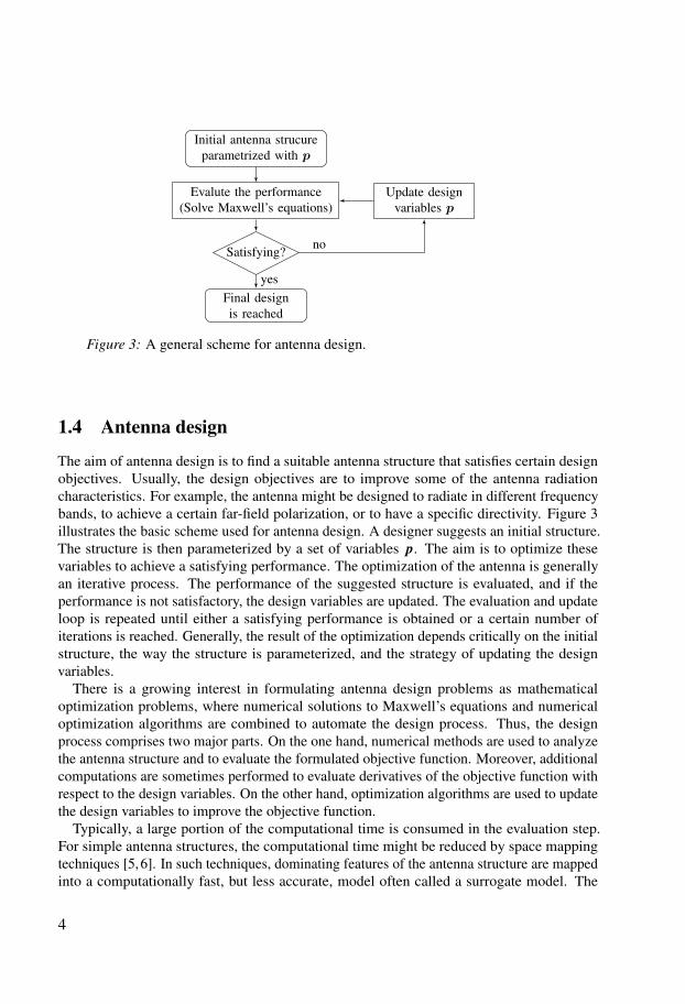
Figure 3: A general scheme for antenna design.
1.4 Antenna design
The aim of antenna design is to find a suitable antenna structure that satisfies certain designobjectives. Usually, the design objectives are to improve some of the antenna radiationcharacteristics. For example, the antenna might be designed to radiate in different frequencybands, to achieve a certain far-field polarization, or to have a specific directivity. Figure 3illustrates the basic scheme used for antenna design. A designer suggests an initial structure.The structure is then parameterized by a set of variables p. The aim is to optimize thesevariables to achieve a satisfying performance. The optimization of the antenna is generallyan iterative process. The performance of the suggested structure is evaluated, and if theperformance is not satisfactory, the design variables are updated. The evaluation and updateloop is repeated until either a satisfying performance is obtained or a certain number ofiterations is reached. Generally, the result of the optimization depends critically on the initialstructure, the way the structure is parameterized, and the strategy of updating the designvariables.
There is a growing interest in formulating antenna design problems as mathematicaloptimization problems, where numerical solutions to Maxwell’s equations and numericaloptimization algorithms are combined to automate the design process. Thus, the designprocess comprises two major parts. On the one hand, numerical methods are used to analyzethe antenna structure and to evaluate the formulated objective function. Moreover, additionalcomputations are sometimes performed to evaluate derivatives of the objective function withrespect to the design variables. On the other hand, optimization algorithms are used to updatethe design variables to improve the objective function.
Typically, a large portion of the computational time is consumed in the evaluation step.For simple antenna structures, the computational time might be reduced by space mappingtechniques [5,6]. In such techniques, dominating features of the antenna structure are mappedinto a computationally fast, but less accurate, model often called a surrogate model. The
4
optimization is carried out mainly using the surrogate model, with the possibility of updatingthat model during the optimization to align with the original problem and capture more physics.However, some antenna structures are too complex to lend their features to a surrogate model.Evaluation of such antennas, therefore, requires accurate solutions to Maxwell’s equations,which are usually computationally expensive. Thus, when optimizing complex antennas, it isessential to use efficient optimization algorithms.
1.5 Optimization algorithmsStaring from an initial guess for the design variables, optimization algorithms seek a solutionof a formulated optimization problem by generating a sequence of updated design variables.In each step of this procedure, optimization algorithms use the available information about theoptimization problem to update the design variables in order to improve the objective function.In electromagnetic design problems, two classes of optimization algorithms are typically used:metaheuristics and gradient-based algorithms.
Metaheuristics are high-level problem-independent heuristic optimization algorithms thatderive heuristic optimization strategies from a metaphor [7]. A metaphor might be a biologicalsystem, individual and collective behavior, or a physical process. Typical examples ofmetaheuristics are genetic algorithms, particle swarm optimization, and simulated annealing[8–11]. Metaheuristics only use information about the value of the objective function, whichmake them simple to use as a black-box software. In these algorithms, the design variablesare updated using heuristics that typically include some stochastic parts. The stochasticparts allow these algorithms to avoid being trapped into a local optimum while searchingfor a solution. Because of their simplicity of use, these methods are frequently used in theelectromagnetic community for design problems that are generally characterized by a smallnumber of design variables [12–14]. Further, most of the commercial software packages usedfor electromagnetic analysis are provided with one or more of those optimization algorithms.However, the small amount of information contained in a usually sparse sampling of objectivefunction values, together with the stochastic parts employed to update the design variables,make metaheuristics inefficient for optimization problems with a large number of designvariables [15].
On the other hand, gradient-based optimization algorithms can efficiently handle optimiza-tion problems that have a large number of design variables. In gradient-based optimizationalgorithms, the design variables are updated based on the necessary conditions of optimalityof the mathematical optimization problems. Information about the objective function andits derivatives with respect to the design variables are used to find the new updates. If theHessian of the objective function (the matrix of second derivatives) is available to a lowcomputational cost, optimization algorithms based on second derivatives, such as Newtonmethods, are preferred because of their fast local convergence. However, computing theHessian of the objective function is often expensive, which is why optimization problems areoften solved by first-order methods such as steepest descent, quasi-Newton, and sequentialconvex approximations methods [16, 17]. First-order methods, besides requiring the objectivefunction value, require the gradient vector (the derivatives of the objective function withrespect to the design variables). The objective function gradient can be evaluated by methods
5

such as finite difference approximations and adjoint-field methods [18–26]. The latter, ifaccessible, are vastly more accurate and efficient to use, especially when the number ofvariables is large. Basic versions of gradient-based optimization algorithms are usually onlylocally convergent; that is, the algorithm will converge to a local optimum if it is initializedsufficiently close to that optimum. By adding a globalization strategy to a locally convergentalgorithm, the algorithm can be made to converge to a local optimum regardless of the initialstarting point [16].
Gradient-based optimization algorithms have been used to solve electromagnetic problemssuch as inverse scattering problems [18–23, 27, 28], filter designs [29–31], and optimizationof magnetic devices [32–35]. However for antenna optimization problems, metaheuristicshave dominated the scene, and only a few works have used gradient-based optimizationalgorithms [36–40]. One reason for this lack of progress is the difficulty in formulatingthe design problem as an optimization problem for which the gradient information can becomputed in an efficient way. Another reason is the tendency of gradient-based methods toconverge to local optima, and it may well happen that the optimization algorithm is trappedin a poor local optimum. Nevertheless, once the optimization problem is formulated, a well-designed gradient-based optimization algorithm will typically find at least a local optimum,which cannot be guaranteed if metaheuristics are used instead.
1.6 Topology optimizationDesign optimization methods can be classified, based on the generality of how the designdomain is parameterized, into three groups: sizing, shape, and topology optimization. Insizing optimization, a structure is parameterized by a set of design variables that express, forinstance, height, width, or thickness of parts of the structure. In shape optimization, the designvariables are used to parameterize the shape of the boundary of a given structure [13, 41–43].
The term topology optimization is often used to label the most general type of designoptimization methods, in which the shapes as well as the connectivity of individual parts of thedevice are subject to design. In topology optimization, design variables are typically used todescribe a function that can spatially describe any structure in one, two, or three dimensionalspace. The most common way of carrying out topology optimization, which is used in thisthesis, is through the material distribution approach. This approach was originally developedto design load-carrying elastic structures [44–47], but the method has been successfullyextended also to other physical disciplines such as acoustics and optics [48–51]. In thisapproach, a density function is used to express the distribution of a material in a given domain.Typically, the density function is sampled into a density vector p D Œp1; p2; ; pM . Eachcomponent pi of the density vector is assigned to an element i in the design domain toindicate presence, pi D 1, or absence, pi D 0, of a material. During the optimization of aparticular objective function, the components of the density vector are allowed to take anyvalue between 0 and 1, but by the end of the process the vector p must hold binary valuesonly, that is, pi D 0 or 1 for all i . Instead of optimizing directly over a density function, analternative topology optimization technique relies on a representation of the geometry throughlevel sets: the device boundary is defined as the zero-level contour of a higher-dimensionalscalar function [52].
6

For topology optimization problems, the number of design variables can easily reachthousands and even millions for 2D and 3D design problems [53, 54]. The large number ofdesign variables means that gradient-based optimization techniques are in practice neededto solve such problems. A main reason for this choice is that the gradient of the objectivefunction contains a massive amount of information, and gradients can in many cases be veryefficiently computed by using solutions of associated adjoint-field problems, as discussed inPaper V. To use gradient-based optimization techniques, the design variables are required tovary continuously between the extreme values (that is, requires pi 2 Œ0; 1 for all i ). However,the appearance of intermediate values (values that are neither 0 nor 1, also called “gray values”)in the final design could lead to ambiguous representation of the obtained design. Techniquessuch as solid isotropic material with penalization (SIMP) [45] or artificial damping [55]can be used to suppress these intermediate values in the final design. In contrast, in thisthesis the intermediate values of the design variables are strongly self-penalized through theoptimization problem formulation itself, and techniques are proposed to promote intermediatevalues during the optimization process.
Topology optimization techniques have been used to design electromagnetic devices byoptimizing permittivity or permeability distributions. For example, topology optimizationhave been used to design magnetic devices by Dyck et al. [32, 33], to design dielectricsubstrates for bandwidth improvement of patch antennas by Kiziltas et al. [36], and to designdielectric resonator antennas to operate with enhanced bandwidth by Nomura et al. [37].Recently, topology optimization using the material distribution approach has been used todesign metallic devices by Erentok and Sigmund [39], where they reported some difficultiesin the interpolation of the conductivity between a good dielectric and a good conductor. Tomitigate the interpolation issue in material distribution problems solved by the finite-elementmethod, Aage et al. [27] proposed an implicit impedance boundary condition, which isalso used by Nomura et al. [31]. Topology optimization of metallic devices has also beenrecently addressed by Zhou et al. [38] and Yamasaki et al. [56], using level set methods. Theprevious contributions to topology optimization of metallic devices, mentioned above, reliedon frequency domain methods, and will therefore be efficient only for the optimization ofdevices operating over a narrow frequency band.
1.7 Finite-difference time-domain method (FDTD)In his 1966 seminal paper [57], Yee introduced a time-domain numerical technique forthe solution of the Maxwell’s equations in first-order form. The algorithm was based ona central-difference approximation of Maxwell’s equations, with staggered grids for theelectric and magnetic fields, solved alternatively at each time step in a leap-frog manner. Allimplementations of the FDTD method at that time suffered from limitations with respectto the termination of unbounded simulation domains. Mur [58] introduced a stable second-order accurate absorbing boundary condition for the FDTD method. Then, the perfectlymatched layer (PML) was introduced by Berenger [59], which solved many of the previouslyproblematic issues with domain termination. Various variants of Berenger’s PML have beenproposed either to ease the numerical implementation or to account for the absorption ofevanescent waves [60, 61].
7

x
y
z
(i,j,k)
Ex(i+12,j,k)
Ey(i,j+ 12,k)
Ez(i,j,k+ 12)
Hx(i,j+ 12,k+ 1
2)
Hy(i+ 12,j,k+ 1
2)
Hz(i+ 12,j+ 1
2,k)∆x
∆y
∆z
1Figure 4: The distribution of the electric and magnetic fields in the basic Yee cell.
Currently, the FDTD method has firmly established itself as one of the most popularmethods in computational electromagnetics. Its popularity is mainly due to:
The ease of implementation.
The efficiency in terms of low memory footprint due to the explicit time stepping.
The wide availability of inexpensive and powerful computing resources such as thegraphics processing units (GPUs).
The increasing interest of modeling inhomogeneous materials.
The wideband data that are potentially available from one simulation.
The FDTD method divides the computational domain into small cubical cells. For eachcell, the six field components are located to match the curl operator. Figure 4 shows Yee’scell for a cube .i; j; k/ with dimension x, y, and z. The electric field componentsare located centered and parallel to the cell edges, while the magnetic field components arelocated centered and normal to the cell faces. Objects are typically represented explicitlyin the Yee grid by their constitutive parameters. The conductivity and the permittivity havethe same spatial distribution as the discretized electric field, and the permeability has thespatial distribution of the discretized magnetic field. The staggered electric and magnetic gridsgive uncertainty about the actual boundary of objects in the Yee grid, and simulated objectstypically have mesh-dependent effective size [62]. More details about the FDTD method canbe found in standard text books [63–65].
Besides being only a second-order-accurate method, a main drawback with the FDTDmethod is the need to use fine grids to accurately model curved objects and small geometricalfeatures. This is due to the Cartesian grid, which leads to a staircase approximation of anygeometry inside the analysis domain. There are several suggested remedies to circumventthe effects of the errors introduced by the staircase approximations, but all generally involve
8

coax
c cd
D
.x/ W
W W
1
out
Wout;1
Win;1
Win,coaxWout,coax
y
z
Figure 5: An illustration of the design problem formulation.
additional arithmetic operations at the boundary cells and sometimes cause instabilities.Generally, the material distribution approach to topology optimization a priori requires thedesign domain to be discretized using fine uniform grids to describe the details of the geometry.This requirement may leave out the main drawbacks of the FDTD method when it is usedwith topology optimization techniques, since the grid size usually need to be small.
2 Thesis summary
This thesis introduces a gradient-based topology optimization approach to design metallicelectromagnetic devices. The focus is to apply the approach to optimize antennas and waveg-uide transitions; however, the approach can be tailored to design various other electromagneticdevices as well.
2.1 Basic problem setup
The basic problem setup is schematically shown in Figure 5. A design domain holdsa conductivity distribution .x/ that defines the conductive parts of a device of unknowntopology, with x representing a point in the design domain. The device could be an antennaor a waveguide transition, depending on whether the analysis domain 1 is an openspace or a waveguide, respectively. A coaxial transmission line couples signals, through anaperture in the xy plane, to and from the analysis domain. The boundary coax is used tointroduce wave energyWin,coax into the coaxial cable, and to measure the wave energyWout,coaxleaving the analysis domain through the coaxial cable. The coaxial cable has an inner corewith diameter d , a metallic shield with diameterD, and is filled with a material with dielectricconstant c and permeability c. Wave energies Win,1 and Wout,1, as illustrated in Figure 5,might enter or leave the analysis domain, respectively, through the boundary out.
9
Inside the analysis domain, assuming no sources inside 1, the 3D Maxwell’s equationsgovern the relation between the electric field E and the magnetic fieldH ,
@
@tH Cr E D 0; (5a)
@
@tE C E r H D 0: (5b)
Inside the lossless coaxial cable, under the assumption that only the TEM mode is supported,the following 1D transport equation is satisfied (PaperII),
@
@t.V ˙ZcI /˙ c
@
@z.V ˙ZcI / D 0; (6)
where V , I , c D 1=pcc, and Zc are the potential difference, the current, the phase velocity,
and the characteristic impedance of the coaxial cable, respectively. The two terms V CZcI
and V ZcI constitute two signals travelling inside the coaxial cable in the positive andnegative z directions, respectively.
Supplied with appropriate initial and boundary conditions, equations (5a), (5b), and (6)can be solved for the electric field E , the magnetic fieldH , the current I , and the potentialdifference V .
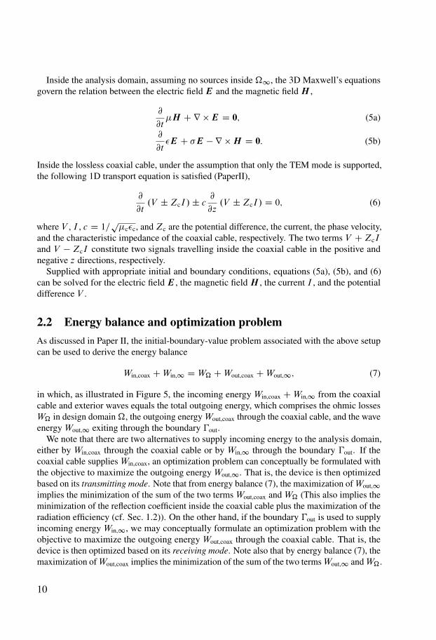
2.2 Energy balance and optimization problemAs discussed in Paper II, the initial-boundary-value problem associated with the above setupcan be used to derive the energy balance
Win,coax CWin,1 D W CWout,coax CWout,1; (7)
in which, as illustrated in Figure 5, the incoming energy Win,coax CWin,1 from the coaxialcable and exterior waves equals the total outgoing energy, which comprises the ohmic lossesW in design domain, the outgoing energyWout,coax through the coaxial cable, and the waveenergy Wout,1 exiting through the boundary out.
We note that there are two alternatives to supply incoming energy to the analysis domain,either by Win,coax through the coaxial cable or by Win,1 through the boundary out. If thecoaxial cable supplies Win,coax, an optimization problem can conceptually be formulated withthe objective to maximize the outgoing energy Wout,1. That is, the device is then optimizedbased on its transmitting mode. Note that from energy balance (7), the maximization ofWout,1implies the minimization of the sum of the two terms Wout,coax and W (This also implies theminimization of the reflection coefficient inside the coaxial cable plus the maximization of theradiation efficiency (cf. Sec. 1.2)). On the other hand, if the boundary out is used to supplyincoming energy Win,1, we may conceptually formulate an optimization problem with theobjective to maximize the outgoing energy Wout,coax through the coaxial cable. That is, thedevice is then optimized based on its receiving mode. Note also that by energy balance (7), themaximization ofWout,coax implies the minimization of the sum of the two termsWout,1 andW.
10

Both formulations thus tend to minimize the losses in order to maximize the correspondingobjective function.
The second alternative is computationally more efficient when time-domain numericalmethods are used, since the full-time history of the observed signal is needed to efficientlycompute the gradient of the objective function by adjoint-field methods, as described inPaper V. Observation of the outgoing signal in the coaxial cable requires less memory thanobservation of the outgoing waves Wout;1. Therefore, the second choice is adopted toformulate the conceptual optimization problem
max.x/2Œmin;max
Wout,coax . .x// ;
s.t. the governing equations;exterior wave sources .Win;1/ ;
Win,coax D 0;
(8)
where min and max represent physical conductivities of a low-loss dielectric and a goodconductor, respectively. The outgoing energy in the coaxial cable can be computed, using thesignal V ZcI in expression (6), as follow
Wout,coax D1
4Zc
Z T
0
.V ZcI /2 dt; (9)
where T denotes the length of the observation time interval.
2.3 Numerical treatmentThe FDTD method is used to numerically solve the time-domain Maxwell’s equations with theopen space radiation condition simulated using a uniaxial perfectly matched layer (UPML) [60,61]. The design variables are the conductivity value at each Yee edge i in the design domain.
Let be a vector that holds the conductivity components at each Yee edge inside thedomain . We introduce the normalized density vector p, whose components are mapped tothe physical conductivities through
i D 10.c1pic2/ S/m; (10)
where the scalars c1 and c2 are selected to control the physical conductivity range Œmin; max.In the numerical experiments in this thesis, we observed a very low sensitivity in the objectivefunction to variations in conductivities below min D 104 S/m or above max D 105 S/m.Therefore, we usually use expression (10) with c1 D 9 and c2 D 4.
Based on the FDTD method, a discrete version of optimization problem (8) can be writtenas
maxp
W out,coax .p/ ;
s.t. the discretized governing equations;
exterior wave sourcesW
in;1
;
W in,coax D 0;
(11)
11

with the discrete objective function defined as
W out,coax.p/ D
1
Zm
NXnD0
.V nC1 OZcInC 1
2z /2t; (12)
where V nC1, InC 1
2z , and OZc are the potential difference, the current, and the characteristic
impedance of the discrete coaxial cable model proposed in Paper II; Zm Dpc=c ; N is
the total number of time steps used in the simulation; and t is the time step used in theFDTD method. An efficient technique to implement the exterior wave sources W
in;1 in theFDTD method is to use the total-field scattered-field formulation [63]. To control the frequencyspectrum of the incoming waves, throughout this thesis, we used a time-domain truncated sincsignal that is usually modulated to the center of the frequency band of interest [66].
To solve optimization problem (11) by a gradient-based optimization algorithm, the gradientof the objective function (12) is required. In Paper V, the adjoint-field method and theFDTD discretization of Maxwell’s equations are used to derive the following expression forthe gradient of objective function (12),
@W out,coax
@iD 3
NXnD1
ENni
En 1
2
i CEnC 1
2
i
2t; (13)
where i denotes the index of an arbitrary Yee-edge inside the design domain; is thespatial discretization step; Ei is the discrete electric field obtained from the FDTD solutionto equations (5) and (6); and Ei is a discrete adjoint electric field obtained by solving anadjoint-field problem. The adjoint-field problem is similar to the FDTD discretization ofequations (5), except that the adjoint-field problem is excited through the boundary coax, atthe bottom of the coaxial cable, using the expression
V n12 C OZcI
n1z D V NnC1 OZcI
NnC 12
z for n D 1; : : : ; N; (14)
where V n12 and I n1z are the discrete potential difference and the current inside the coaxial
cable of the adjoint problem. Note that the left side of expression (14) constitutes a signalpropagating inside the coaxial cable in the positive z direction, and that the right side is thetime-reversed signal that propagates in the negative z direction for the original-field problem.In other words, the time-reversed received signal in the original-field problem constitutes theincoming signal for the adjoint-field problem.
Thus, by using two FDTD solutions, the objective function and the gradient vector canbe computed for any number of design variables inside the design domain . In this thesis,the globally convergent method of moving asymptotes (GCMMA) [67] is used to updatethe design variables. The GCMMA is a first-order gradient-based optimization method thatbelong to the class of sequential convex approximation methods [17, ch4].
12
σmin σmaxσmed
0
0.2
0.4
0.6
0.8
1
Conductivity (S/m)
Norm
alized
energy
loss
∗ ∗∗ ∗
∗∗∗∗ ∗
∗ ∗∗ ∗ ∗
∗ ∗ ∗ ∗ ∗ ∗∗∗∗∗∗∗ ∗
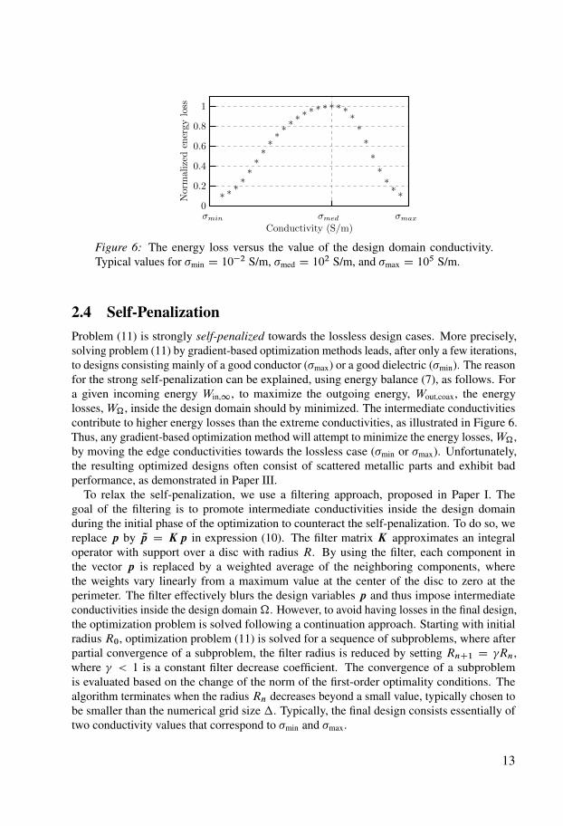
Figure 6: The energy loss versus the value of the design domain conductivity.Typical values for min D 10
2 S/m, med D 102 S/m, and max D 10
5 S/m.
2.4 Self-PenalizationProblem (11) is strongly self-penalized towards the lossless design cases. More precisely,solving problem (11) by gradient-based optimization methods leads, after only a few iterations,to designs consisting mainly of a good conductor (max) or a good dielectric (min). The reasonfor the strong self-penalization can be explained, using energy balance (7), as follows. Fora given incoming energy Win,1, to maximize the outgoing energy, Wout,coax, the energylosses, W, inside the design domain should by minimized. The intermediate conductivitiescontribute to higher energy losses than the extreme conductivities, as illustrated in Figure 6.Thus, any gradient-based optimization method will attempt to minimize the energy losses,W,by moving the edge conductivities towards the lossless case (min or max). Unfortunately,the resulting optimized designs often consist of scattered metallic parts and exhibit badperformance, as demonstrated in Paper III.
To relax the self-penalization, we use a filtering approach, proposed in Paper I. Thegoal of the filtering is to promote intermediate conductivities inside the design domainduring the initial phase of the optimization to counteract the self-penalization. To do so, wereplace p by Qp D Kp in expression (10). The filter matrix K approximates an integraloperator with support over a disc with radius R. By using the filter, each component inthe vector p is replaced by a weighted average of the neighboring components, wherethe weights vary linearly from a maximum value at the center of the disc to zero at theperimeter. The filter effectively blurs the design variables p and thus impose intermediateconductivities inside the design domain. However, to avoid having losses in the final design,the optimization problem is solved following a continuation approach. Starting with initialradius R0, optimization problem (11) is solved for a sequence of subproblems, where afterpartial convergence of a subproblem, the filter radius is reduced by setting RnC1 D Rn,where < 1 is a constant filter decrease coefficient. The convergence of a subproblemis evaluated based on the change of the norm of the first-order optimality conditions. Thealgorithm terminates when the radius Rn decreases beyond a small value, typically chosen tobe smaller than the numerical grid size . Typically, the final design consists essentially oftwo conductivity values that correspond to min and max.
13

Initialdistribution p
Filtering of designvariables p and mapping to σ
Compute objective(solve Maxwell’s equations)
Compute gradient(solve adjoint Maxwell’s equ.)
Filter the gradient (chain rule)
Upd
ate
desi
gnva
riab
les
(GC
MM
A)
Converged?
Upd
ate
filte
rra
diusR
n+1
=γR
n
Rn<∆
Final design σ
yes
yes
no
no
Figure 7: A flowchart of the optimization process.
2.5 Summary of the optimization processThe flowchart in Figure 7 illustrates the optimization process. The process starts with a uniforminitial distribution of the design variables, p, which typically corresponds to a conductivityaround the peak in Figure 6. Starting with an initial filter radius R0, the optimization problemis solved through solutions to a number of subproblems. In each subproblem, the designvariables are filtered and mapped to the physical conductivities . Then the FDTD methodnumerically solves Maxwell’s equations and the associated adjoint-field problem in orderto compute the objective function and the gradient vector. The chain rule is used to obtainthe gradient with respect to the design variables p. Then a convergence criterion based onthe first-order necessary condition is tested. If the convergence criterion is not satisfied, theoptimization process continues to a new cycle in the current subproblem, where the GCMMAalgorithm use the gradient and the objective function values to update the design variables.The GCMMA might evaluate the objective function a few additional times to find updatesthat satisfy a sufficient improvement condition of the objective function. If the convergencecriterion is reached but the filter radius is greater than Q D =
p2, the minimal distance
between two conductivity components in the Yee grid, the radius of the filter is reduced,RnC1 D Rn, and a new subproblem starts. Finally, the optimization process terminatesif the convergence criterion is satisfied and the filter radius is smaller than or equal to Q.Typically, the optimized design consists of conductivities that are either min or max. In a
14

1 2 3 4 5 6 7 8 9 10−30
−25
−20
−15
−10
−5
0
5
|S11| (
dB
)
Frequency (GHz)
Optimized design Reference
Figure 8: Left: the final conductivity distribution of the monopole designed based onlinearly-polarized plane wave excitation. The optimization problem has 20; 200 de-sign variables (the coaxial cable connection point is marked by a gray dot). Right:the reflection coefficient of the antenna.
final step before evaluating the performance of the optimized design, a threshold conductivityth D 0:1 S/m is usually used to map conductivities below and above th to 0 S/m (void) and5:8 107 S/m (copper), respectively.
2.6 Selected results
2.6.1 Ultrawideband (UWB) monopole design
Recently, UWB antennas have received great attention in applications such as wirelesscommunication and high resolution radar [68, 69]. A key candidate for UWB antennas isthe planar monopole. In Paper I, optimization problem (11) is used for the complete layoutoptimization of the radiating element of planar monopole antennas. We use a design domainthat has an area of 75 75 mm2, located 0:75 mm above a simulated infinite ground plane,and connected at the center of its bottom side to a 50 coaxial cable. The design domainis discretized into 100 100 Yee cell faces, which yields 20; 200 design variables (oneconductivity component for each Yee edge). The objective is to maximize the energy receivedby the planar monopole over the frequency band 1–10 GHz.
The analysis domain is excited by a set of external sources that surround the monopoleand radiate linearly-polarized plane waves. Figure 8 shows the final design obtained by theoptimization algorithm in 132 iterations. The final design uses only around 50 45 mm2
out of the available design domain area. The reflection coefficient jS11j of the optimizedmonopole is below 10 dB over the frequency band 1:2 8:5 GHz. Included in the same
15
1 2 3 4 5 6 7 8 9 10−30
−25
−20
−15
−10
−5
0
5
|S11| (
dB
)
Frequency (GHz)
1 2 3 4 5 6 7 8 9 10
90
92
94
96
98
100
Rad
iati
on e
ffic
iency
(%
)
|S11|(FDTD)|S11|(CST)
Efficiency (CST)
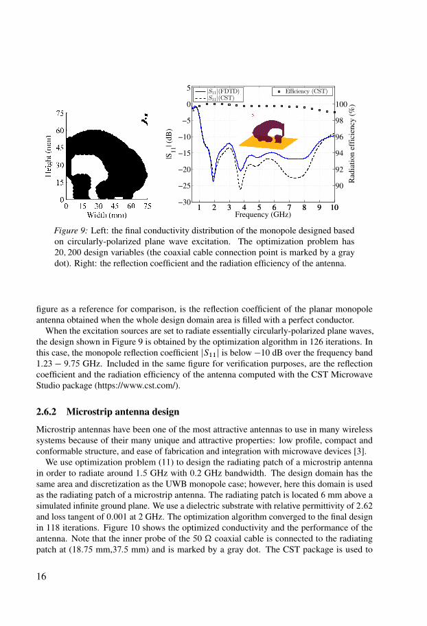
Figure 9: Left: the final conductivity distribution of the monopole designed basedon circularly-polarized plane wave excitation. The optimization problem has20; 200 design variables (the coaxial cable connection point is marked by a graydot). Right: the reflection coefficient and the radiation efficiency of the antenna.
figure as a reference for comparison, is the reflection coefficient of the planar monopoleantenna obtained when the whole design domain area is filled with a perfect conductor.
When the excitation sources are set to radiate essentially circularly-polarized plane waves,the design shown in Figure 9 is obtained by the optimization algorithm in 126 iterations. Inthis case, the monopole reflection coefficient jS11j is below 10 dB over the frequency band1:23 9:75 GHz. Included in the same figure for verification purposes, are the reflectioncoefficient and the radiation efficiency of the antenna computed with the CST MicrowaveStudio package (https://www.cst.com/).
2.6.2 Microstrip antenna design
Microstrip antennas have been one of the most attractive antennas to use in many wirelesssystems because of their many unique and attractive properties: low profile, compact andconformable structure, and ease of fabrication and integration with microwave devices [3].
We use optimization problem (11) to design the radiating patch of a microstrip antennain order to radiate around 1:5 GHz with 0:2 GHz bandwidth. The design domain has thesame area and discretization as the UWB monopole case; however, here this domain is usedas the radiating patch of a microstrip antenna. The radiating patch is located 6 mm above asimulated infinite ground plane. We use a dielectric substrate with relative permittivity of 2:62and loss tangent of 0:001 at 2 GHz. The optimization algorithm converged to the final designin 118 iterations. Figure 10 shows the optimized conductivity and the performance of theantenna. Note that the inner probe of the 50 coaxial cable is connected to the radiatingpatch at (18:75 mm,37:5 mm) and is marked by a gray dot. The CST package is used to
16

0 15 30 45 60 750
15
30
45
60
75
Width (mm)
Len
gth
(mm
)
1 1.25 1.5 1.75 2 2.25 2.5−30
−25
−20
−15
−10
−5
0
5
|S1
1| (
dB
)
Frequency (GHz)
1 1.25 1.5 1.75 2 2.25 2.5
80
84
88
92
96
100
Rad
iati
on e
ffic
iency
(%
)
|S11|(FDTD)|S11|(CST)
Efficiency (CST)
Figure 10: Left: the final conductivity distribution over the patch area of themicrostrip antenna optimized to radiate at 1:5 GHz (the probe connection point ismarked by a gray dot). Right: the reflection coefficient and the radiation efficiency.
1 1.25 1.5 1.75 2 2.25 2.5−30
−25
−20
−15
−10
−5
0
5
|S11| (
dB
)
Frequency (GHz)
1 1.25 1.5 1.75 2 2.25 2.5
80
84
88
92
96
100
Rad
iati
on e
ffic
ien
cy (
%)
|S11|(FDTD)|S11|(CST)
Efficiency (CST)
Figure 11: Left: the final conductivity distribution over the patch area of themicrostrip antenna that radiates over two frequency bands centered around 1:5 GHzand 2 GHz (the probe connection point is marked by a gray dot). Right: thereflection coefficient and the radiation efficiency.
17
0 15 30 45 60 75 90 1050
15
30
45
60
75
90
105
Width (mm)
Len
gth
(mm
)
0 15 30 45 60 75 90 1050
15
30
45
60
75
90
105
Width (mm)
Len
gth
(mm
)
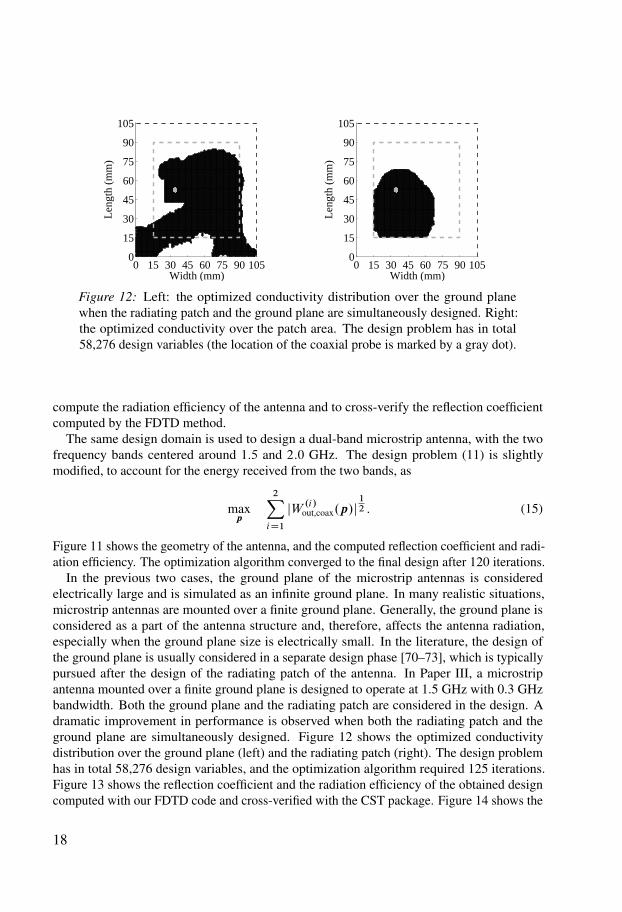
Figure 12: Left: the optimized conductivity distribution over the ground planewhen the radiating patch and the ground plane are simultaneously designed. Right:the optimized conductivity over the patch area. The design problem has in total58,276 design variables (the location of the coaxial probe is marked by a gray dot).
compute the radiation efficiency of the antenna and to cross-verify the reflection coefficientcomputed by the FDTD method.
The same design domain is used to design a dual-band microstrip antenna, with the twofrequency bands centered around 1:5 and 2:0 GHz. The design problem (11) is slightlymodified, to account for the energy received from the two bands, as
maxp
2XiD1
jW.i/
out,coax.p/j12 : (15)
Figure 11 shows the geometry of the antenna, and the computed reflection coefficient and radi-ation efficiency. The optimization algorithm converged to the final design after 120 iterations.
In the previous two cases, the ground plane of the microstrip antennas is consideredelectrically large and is simulated as an infinite ground plane. In many realistic situations,microstrip antennas are mounted over a finite ground plane. Generally, the ground plane isconsidered as a part of the antenna structure and, therefore, affects the antenna radiation,especially when the ground plane size is electrically small. In the literature, the design ofthe ground plane is usually considered in a separate design phase [70–73], which is typicallypursued after the design of the radiating patch of the antenna. In Paper III, a microstripantenna mounted over a finite ground plane is designed to operate at 1.5 GHz with 0.3 GHzbandwidth. Both the ground plane and the radiating patch are considered in the design. Adramatic improvement in performance is observed when both the radiating patch and theground plane are simultaneously designed. Figure 12 shows the optimized conductivitydistribution over the ground plane (left) and the radiating patch (right). The design problemhas in total 58,276 design variables, and the optimization algorithm required 125 iterations.Figure 13 shows the reflection coefficient and the radiation efficiency of the obtained designcomputed with our FDTD code and cross-verified with the CST package. Figure 14 shows the
18
1 1.2 1.4 1.6 1.8 2−30
−25
−20
−15
−10
−5
0
5
|S11| (
dB
)
Frequency (GHz)
1 1.2 1.4 1.6 1.8 2
90
92
94
96
98
100
Rad
iati
on
eff
icie
ncy
(%
)
|S11|(FDTD)|S11|(CST)
Efficiency (FDTD)Efficiency (CST)
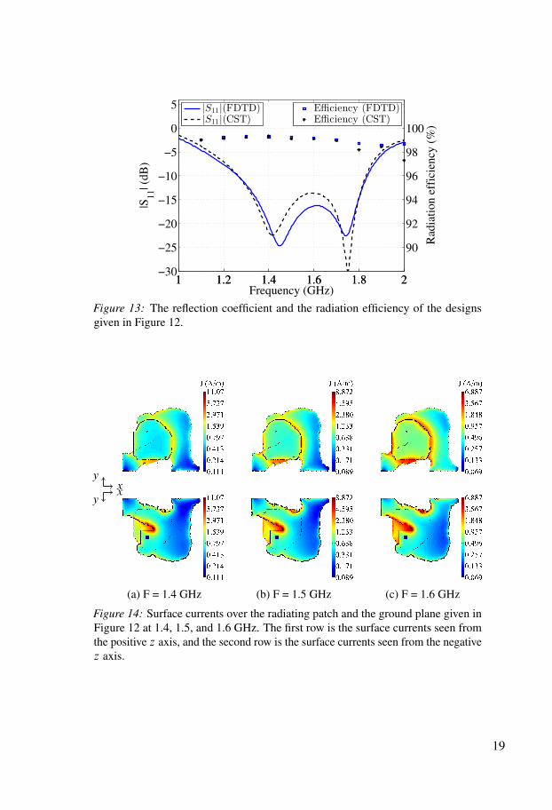
Figure 13: The reflection coefficient and the radiation efficiency of the designsgiven in Figure 12.
(a) F = 1.4 GHz (b) F = 1.5 GHz (c) F = 1.6 GHz
xy
xy
Figure 14: Surface currents over the radiating patch and the ground plane given inFigure 12 at 1.4, 1.5, and 1.6 GHz. The first row is the surface currents seen fromthe positive z axis, and the second row is the surface currents seen from the negativez axis.
19
dfy
z
x
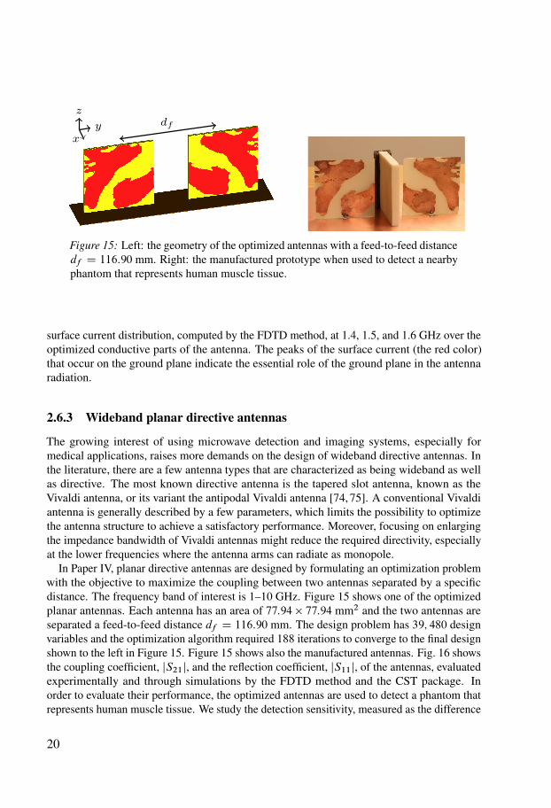
Figure 15: Left: the geometry of the optimized antennas with a feed-to-feed distancedf D 116:90 mm. Right: the manufactured prototype when used to detect a nearbyphantom that represents human muscle tissue.
surface current distribution, computed by the FDTD method, at 1.4, 1.5, and 1.6 GHz over theoptimized conductive parts of the antenna. The peaks of the surface current (the red color)that occur on the ground plane indicate the essential role of the ground plane in the antennaradiation.
2.6.3 Wideband planar directive antennas
The growing interest of using microwave detection and imaging systems, especially formedical applications, raises more demands on the design of wideband directive antennas. Inthe literature, there are a few antenna types that are characterized as being wideband as wellas directive. The most known directive antenna is the tapered slot antenna, known as theVivaldi antenna, or its variant the antipodal Vivaldi antenna [74, 75]. A conventional Vivaldiantenna is generally described by a few parameters, which limits the possibility to optimizethe antenna structure to achieve a satisfactory performance. Moreover, focusing on enlargingthe impedance bandwidth of Vivaldi antennas might reduce the required directivity, especiallyat the lower frequencies where the antenna arms can radiate as monopole.
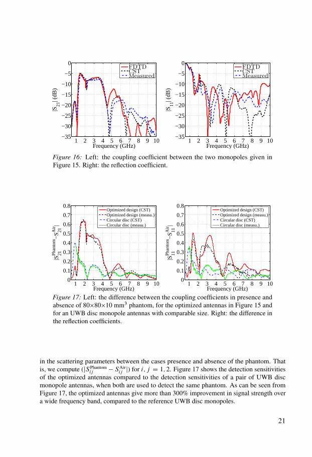
In Paper IV, planar directive antennas are designed by formulating an optimization problemwith the objective to maximize the coupling between two antennas separated by a specificdistance. The frequency band of interest is 1–10 GHz. Figure 15 shows one of the optimizedplanar antennas. Each antenna has an area of 77:94 77:94 mm2 and the two antennas areseparated a feed-to-feed distance df D 116:90 mm. The design problem has 39; 480 designvariables and the optimization algorithm required 188 iterations to converge to the final designshown to the left in Figure 15. Figure 15 shows also the manufactured antennas. Fig. 16 showsthe coupling coefficient, jS21j, and the reflection coefficient, jS11j, of the antennas, evaluatedexperimentally and through simulations by the FDTD method and the CST package. Inorder to evaluate their performance, the optimized antennas are used to detect a phantom thatrepresents human muscle tissue. We study the detection sensitivity, measured as the difference
20
1 2 3 4 5 6 7 8 9 10−35
−30
−25
−20
−15
−10
−5
0
|S21
| (dB
)
Frequency (GHz)
FDTDCSTMeasured
1 2 3 4 5 6 7 8 9 10−35
−30
−25
−20
−15
−10
−5
0
|S11
| (dB
)
Frequency (GHz)
FDTDCSTMeasured
Figure 16: Left: the coupling coefficient between the two monopoles given inFigure 15. Right: the reflection coefficient.
1 2 3 4 5 6 7 8 9 100
0.1
0.2
0.3
0.4
0.5
0.6
0.7
0.8
|S21P
hant
om−
S 21Air|
Frequency (GHz)
Optimized design (CST)Optimized design (measu.)Circular disc (CST)Circular disc (measu.)
1 2 3 4 5 6 7 8 9 100
0.1
0.2
0.3
0.4
0.5
0.6
0.7
0.8
|S11P
hant
om−
S 11Air|
Frequency (GHz)
Optimized design (CST)Optimized design (measu.)Circular disc (CST)Circular disc (measu.)
Figure 17: Left: the difference between the coupling coefficients in presence andabsence of 808010 mm3 phantom, for the optimized antennas in Figure 15 andfor an UWB disc monopole antennas with comparable size. Right: the difference inthe reflection coefficients.
in the scattering parameters between the cases presence and absence of the phantom. Thatis, we compute (jSPhantom
ij SAirij j) for i; j D 1; 2. Figure 17 shows the detection sensitivities
of the optimized antennas compared to the detection sensitivities of a pair of UWB discmonopole antennas, when both are used to detect the same phantom. As can be seen fromFigure 17, the optimized antennas give more than 300% improvement in signal strength overa wide frequency band, compared to the reference UWB disc monopoles.
21
ΩWin,wg
Wout,wgb
a
(A) End-launcher transition
Wout,coax
Win,coax
(B) Right-angle transition
Wou
t,coa
x
Win
,coa
x
zx
y
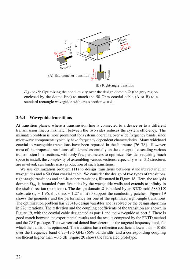
Figure 18: Optimizing the conductivity over the design domain (the gray regionenclosed by the dotted line) to match the 50 Ohm coaxial cable (A or B) to astandard rectangle waveguide with cross section a b.
2.6.4 Waveguide transitions
At transition planes, where a transmission line is connected to a device or to a differenttransmission line, a mismatch between the two sides reduces the system efficiency. Themismatch problem is more prominent for systems operating over wide frequency bands, sincemicrowave components typically have frequency dependent characteristics. Many widebandcoaxial-to-waveguide transitions have been reported in the literature [76–78]. However,most of the proposed transitions still depend essentially on the concept of cascading varioustransmission line sections, with only few parameters to optimize. Besides requiring muchspace to install, the complexity of assembling various sections, especially when 3D structuresare involved, can hinder mass production of such transitions.
We use optimization problem (11) to design transitions between standard rectangularwaveguides and a 50 Ohm coaxial cable. We consider the design of two types of transitions,right-angle transitions and end-launcher transitions, illustrated in Figure 18. Here, the analysisdomain 1 is bounded from five sides by the waveguide walls and extends to infinity inthe sixth direction (positive z). The design domain is backed by an RT/Duroid 5880 LZsubstrate (r = 1.96, thickness = 1.27 mm) to support the conducting patches. Figure 19shows the geometry and the performance for one of the optimized right-angle transitions.The optimization problem has 28; 410 design variables and is solved by the design algorithmin 226 iterations. The reflection and the coupling coefficients of the transition are shown inFigure 19, with the coaxial cable designated as port 1 and the waveguide as port 2. There isgood match between the experimental results and the results computed by the FDTD methodand the CST package. The two vertical dotted lines determine the targeted frequency band, forwhich the transition is optimized. The transition has a reflection coefficient lower than 10 dBover the frequency band 6:75–13:5 GHz (66% bandwidth) and a corresponding couplingcoefficient higher than 0:5 dB. Figure 20 shows the fabricated prototype.
22

0.00 5.71 11.43 17.14 22.860.00
2.54
5.08
7.62
10.16
Hei
ght (
mm
)
Depth (mm)
z
x
5 6 7 8 9 10 11 12 13 14 15−50
−40
−30
−20
−10
0
Am
plitu
de (
dB)
Frequency (GHz)
5 6 7 8 9 10 11 12 13 14 15
−240
−120
0
120
240
P
hase
(de
gree
)
|S11|(FDTD)|S11|(CST)|S11|(Meas.)|S21|(CST) 6 S21 (CST)
Figure 19: Left: the optimized conductivity distribution enclosed by three of thewaveguide walls and the dashed line. Right: the scattering parameters of theright-angle transition.
−15 −10 −5 0 5 10 15
−5
0
5
(mm)
Figure 20: Left: the fabricated prototype of the optimized design backed by theRT/Duroid 5880 LZ substrate. Right: the assembled right-angle transition (theshorting wall at z D 0 is removed for visibility).
23

References[1] IEEE Standard for Definitions of Terms for Antennas, IEEE Std 145-2013, 2014.
[2] C. A. Balanis, Advanced Engineering Electromagnetics. John Wiley & Sons, 1989.
[3] ——, Antenna Theory: Analysis and Design, 3rd ed. Wiley-Interscience, 2005.
[4] M. N. Sadiku, Numerical Techniques in Electromagnetics, 2nd ed. CRC Press, 2001.
[5] J. Zhu, J. Bandler, N. Nikolova, and S. Koziel, “Antenna optimization through spacemapping,” IEEE Trans. Antennas Propag., vol. 55, no. 3, pp. 651–658, March 2007.
[6] S. Koziel, S. Ogurtsov, J. Bandler, and Q. Cheng, “Reliable space-mapping optimizationintegrated with EM-based adjoint sensitivities,” IEEE Trans. Microw. Theory Tech.,vol. 61, no. 10, pp. 3493–3502, Oct 2013.
[7] K. Sörensen, “Metaheuristics–the metaphor exposed,” Int. Trans. in Op. Res., vol. 22,no. 1, pp. 3–18, 2015.
[8] R. L. Haupt, “An introduction to genetic algorithms for electromagnetics,” IEEE Anten-nas Propag. Mag., vol. 37, no. 2, pp. 7–15, 1995.
[9] J. Robinson and Y. Rahmat-Samii, “Particle swarm optimization in electromagnetics,”IEEE Trans. Antennas Propag., vol. 52, no. 2, pp. 397–407, Feb 2004.
[10] S. Kirkpatrick, C. D. Gelatt, and M. P. Vecchi, “Optimization by simulated annealing,”Science, vol. 220, no. 4598, pp. 671–680, 1983.
[11] J. Perez and J. Basterrechea, “Comparison of different heuristic optimization methodsfor near-field antenna measurements,” IEEE Trans. Antennas Propag., vol. 55, no. 3, pp.549 –555, Mar. 2007.
[12] M. John and M. Ammann, “Wideband printed monopole design using a genetic algo-rithm,” IEEE Antennas Wireless Propag. Lett., vol. 6, pp. 447 –449, 2007.
[13] L. Griffiths, C. Furse, and Y. C. Chung, “Broadband and multiband antenna design usingthe genetic algorithm to create amorphous shapes using ellipses,” IEEE Trans. AntennasPropag., vol. 54, no. 10, pp. 2776 –2782, Oct. 2006.
[14] F. Villegas, T. Cwik, Y. Rahmat-Samii, and M. Manteghi, “A parallel electromagneticgenetic-algorithm optimization (EGO) application for patch antenna design,” IEEETrans. Antennas Propag., vol. 52, no. 9, pp. 2424 – 2435, Sep. 2004.
[15] O. Sigmund, “On the usefulness of non-gradient approaches in topology optimization,”Struct. Multidiscip. Optim., vol. 43, pp. 589–596, 2011.
[16] J. Nocedal and S. Wright, Numerical optimization. Springer-Verlag New York, 1999.
24

[17] P. Christensen and A. Klarbring, An Introduction to Structural Optimization. SpringerNetherlands, 2008.
[18] M. Gustafsson and S. He, “An optimization approach to two-dimensional time domainelectromagnetic inverse problems,” Radio Science, vol. 35, no. 2, pp. 525–536, Mar.2000.
[19] Y.-S. Chung, C. Cheon, and S.-Y. Hahn, “Reconstruction of dielectric cylinders usingFDTD and topology optimization technique,” IEEE Trans. Magn., vol. 36, no. 4, pp.956–959, Jul 2000.
[20] Y.-S. Chung, C. Cheon, I.-H. Park, and S.-Y. Hahn, “Optimal design method for mi-crowave device using time domain method and design sensitivity analysis. II. FDTDcase,” IEEE Trans. Magn., vol. 37, no. 5, pp. 3255 –3259, Sep. 2001.
[21] I. Rekanos, “Inverse scattering in the time domain: an iterative method using an FDTDsensitivity analysis scheme,” IEEE Trans. Magn., vol. 38, no. 2, pp. 1117–1120, Mar2002.
[22] E. Abenius and B. Strand, “Solving inverse electromagnetic problems using FDTD andgradient-based minimization,” Int. J. Num. Meth. Eng., vol. 68, no. 6, pp. 650–673,2006.
[23] P. Jacobsson and T. Rylander, “Gradient-based shape optimisation of conformal arrayantennas,” IET Microw. Antennas Propag., vol. 4, no. 2, pp. 200–209, Feb. 2010.
[24] N. Nikolova, H. Tam, and M. Bakr, “Sensitivity analysis with the FDTD method onstructured grids,” IEEE Trans. Microw. Theory Tech., vol. 52, no. 4, pp. 1207 – 1216,Apr. 2004.
[25] A. Bondeson, Y. Yang, and P. Weinerfelt, “Shape optimization for radar cross sectionsby a gradient method,” Int. J. Num. Meth. Eng., vol. 61, no. 5, pp. 687–715, 2004.
[26] M. H. Bakr, O. S. Ahmed, M. H. E. Sherif, and T. Nomura, “Time domain adjointsensitivity analysis of electromagnetic problems with nonlinear media,” Opt. Express,vol. 22, no. 9, pp. 10 831–10 843, May 2014.
[27] N. Aage, N. A. Mortensen, and O. Sigmund, “Topology optimization of metallic devicesfor microwave applications,” Int. J. Num. Meth. Eng., vol. 83, no. 2, pp. 228–248, 2010.
[28] A. Diaz and O. Sigmund, “A topology optimization method for design of negativepermeability metamaterials,” Struct. Multidiscip. Optim., vol. 41, pp. 163–177, 2010.
[29] H. Khalil, A. Assadihaghi, S. Bila, D. Baillargeat, M. Aubourg, S. Verdeyme, J. Puech,and L. Lapierre, “Topology gradient optimization in 2-D and 3-D for the design ofmicrowave components,” Microw. Opt. Technol. Lett., vol. 50, no. 10, pp. 2739–2743,2008.
25

[30] S. Koziel, F. Mosler, S. Reitzinger, and P. Thoma, “Robust microwave designoptimization using adjoint sensitivity and trust regions,” Int. J. Rf. Microw. C. E., vol. 22,no. 1, pp. 10–19, 2012.
[31] T. Nomura, M. Ohkado, P. Schmalenberg, J. Lee, O. Ahmed, and M. Bakr, “Topologyoptimization method for microstrips using boundary condition representation and adjointanalysis,” in EuMC2013, Oct 2013, pp. 632–635.
[32] D. Dyck, D. Lowther, and E. Freeman, “A method of computing the sensitivity ofelectromagnetic quantities to changes in materials and sources,” IEEE Trans. Magn.,vol. 30, no. 5, pp. 3415 –3418, Sep. 1994.
[33] D. Dyck and D. Lowther, “Automated design of magnetic devices by optimizing materialdistribution,” IEEE Trans. Magn., vol. 32, no. 3, pp. 1188 –1193, May 1996.
[34] T. Labbé and B. Dehez, “Convexity-oriented method for the topology optimization offerromagnetic moving parts in electromagnetic actuators using magnetic energy,” IEEETrans. Magn., vol. 46, no. 12, pp. 4016–4022, Dec 2010.
[35] M. Otomori, T. Yamada, K. Izui, S. Nishiwaki, and N. Kogiso, “Level set-based topologyoptimization for the design of a ferromagnetic waveguide,” IEEE Trans. Magn., vol. 48,no. 11, pp. 3072–3075, Nov 2012.
[36] G. Kiziltas, D. Psychoudakis, J. Volakis, and N. Kikuchi, “Topology design optimizationof dielectric substrates for bandwidth improvement of a patch antenna,” IEEE Trans.Antennas Propag., vol. 51, no. 10, pp. 2732 – 2743, Oct. 2003.
[37] T. Nomura, K. Sato, K. Taguchi, T. Kashiwa, and S. Nishiwaki, “Structural topologyoptimization for the design of broadband dielectric resonator antennas using the finitedifference time domain technique,” Int. J. Num. Meth. Eng., vol. 71, pp. 1261–1296,2007.
[38] S. Zhou, W. Li, and Q. Li, “Level-set based topology optimization for electromagneticdipole antenna design,” J. Comput. Phys., vol. 229, no. 19, pp. 6915 – 6930, 2010.
[39] A. Erentok and O. Sigmund, “Topology optimization of sub-wavelength antennas,” IEEETrans. Antennas Propag., vol. 59, no. 1, pp. 58 –69, Jan. 2011.
[40] M. Ghassemi, M. Bakr, and N. Sangary, “Antenna design exploiting adjoint sensitivity-based geometry evolution,” IET Microw. Antennas Propag., vol. 7, no. 4, pp. 268–276,Mar. 2013.
[41] P. Jacobsson and T. Rylander, “Shape optimization of the total scattering cross sectionfor cylindrical scatterers,” Radio Science, vol. 44, no. 4, Aug. 2009.
[42] N. Uchida, S. Nishiwaki, K. Izui, M. Yoshimura, T. Nomura, and K. Sato, “Simultaneousshape and topology optimization for the design of patch antennas,” in EuCAP 2009, Mar.2009, pp. 103–107.
26
[43] J. Kataja, S. Jarvenpää, J. Toivanen, R. Mäkinen, and P. Ylä-Oijala, “Shape sensitivityanalysis and gradient-based optimization of large structures using MLFMA,” IEEETrans. Antennas Propag., vol. 62, no. 11, pp. 5610–5618, Nov. 2014.
[44] M. P. Bendsøe and N. Kikuchi, “Generating optimal topologies in structural designusing a homogenization method,” Comput. Methods in Appl. Mech. Eng., vol. 71, no. 2,pp. 197–224, 1988.
[45] M. P. Bendsøe and O. Sigmund, Topology Optimization. Theory, Methods, and Applica-tions. Springer, 2003.
[46] O. Sigmund and K. Maute, “Topology optimization approaches,” Struct. Multidiscip.Optim., vol. 48, no. 6, pp. 1031–1055, 2013.
[47] J. Deaton and R. Grandhi, “A survey of structural and multidisciplinary continuumtopology optimization: post 2000,” Struct. Multidiscip. Optim., vol. 49, no. 1, pp. 1–38,2014.
[48] E. Wadbro, “Analysis and design of acoustic transition sections for impedance matchingand mode conversion,” Struct. Multidiscip. Optim., vol. 50, no. 3, pp. 395–408, 2014.
[49] J. Jensen and O. Sigmund, “Topology optimization for nano-photonics,” Laser Photon.Rev., vol. 5, no. 2, pp. 308–321, 2011.
[50] Y.-S. Chung, B.-J. Lee, and S.-C. Kim, “Optimal shape design of dielectric micro lensusing FDTD and topology optimization,” J. Opt. Soc. Korea, vol. 13, no. 2, pp. 286–293,Jun. 2009.
[51] J. Andkjær, V. Johansen, K. Friis, and O. Sigmund, “Inverse design of nanostructuredsurfaces for color effects,” J. Opt. Soc. Am. B, vol. 31, no. 1, pp. 164–174, 2014.
[52] G. Allaire, F. Jouve, and A.-M. Toader, “A level-set method for shape optimization,” C.R. Acad. Sci. Paris Sér. I Math., vol. 334, no. 12, pp. 1125–1130, 2002.
[53] E. Wadbro and M. Berggren, “Megapixel topology optimization on a graphicsprocessing unit,” SIAM Review, vol. 51, no. 4, pp. 707–721, 2009.
[54] N. Aage and B. Lazarov, “Parallel framework for topology optimization using themethod of moving asymptotes,” Struct. Multidiscip. Optim., vol. 47, no. 4, pp. 493–505,2013.
[55] J. Jensen, O. Sigmund, L. H. Frandsen, P. I. Borel, A. Harpoth, and M. Kristensen,“Topology design and fabrication of an efficient double 900 photonic crystal waveguidebend,” IEEE Photon. Technol. Lett., vol. 17, no. 6, pp. 1202–1204, 2005.
[56] S. Yamasaki, T. Nomura, A. Kawamoto, K. Sato, and S. Nishiwaki, “A level set-basedtopology optimization method targeting metallic waveguide design problems,” Int. J.Num. Meth. Eng., vol. 87, no. 9, pp. 844–868, 2011.
27

[57] K. Yee, “Numerical solution of initial boundary value problems involving Maxwell’sequations in isotropic media,” IEEE Trans. Antennas Propag., vol. 14, no. 3, pp. 302–307, May 1966.
[58] G. Mur, “Absorbing boundary conditions for the finite-difference approximation ofthe time-domain electromagnetic-field equations,” IEEE Trans. Electromagn. Compat.,vol. 23, no. 4, pp. 377–382, 1981.
[59] J.-P. Berenger, “A perfectly matched layer for the absorption of electromagnetic waves,”J. Comput. Phys., vol. 114, no. 2, pp. 185–200, 1994.
[60] S. Gedney, “An anisotropic perfectly matched layer-absorbing medium for the truncationof FDTD lattices,” IEEE Trans. Antennas Propag., vol. 44, no. 12, pp. 1630 –1639, Dec.1996.
[61] J. Fang and Z. Wu, “Generalized perfectly matched layer for the absorption of propa-gating and evanescent waves in lossless and lossy media,” IEEE Trans. Microw. TheoryTech., vol. 44, no. 12, pp. 2216–2222, Dec. 1996.
[62] N. Farahat and R. Mittra, “Analysis of frequency selective surfaces using the finitedifference time domain (FDTD) method,” in IEEE AP-S Int. Symp., vol. 2, 2002, pp.568–571.
[63] A. Taflove and S. Hagness, Computational Electrodynamics: The Finite-DifferenceTime-Domain Method, 3rd ed. Artech House, 2005.
[64] A. Elsherbeni and V. Demir, The Finite Difference Time Domain Method forElectromagnetics: With MATLAB Simulations. SciTech Publishing, Inc., 2009.
[65] U. S. Inan and R. A. Marshall, Numerical Electromagnetics: The FDTD Method.Cambridge University Press, 2011.
[66] B. P. Lathi, Modern Digital and Analog Communication Systems, 3rd ed. OxfordUniversity Press, 1998.
[67] K. Svanberg, “A class of globally convergent optimization methods based onconservative convex separable approximations,” SIAM J. Optim., vol. 12, no. 2, pp.555–573, 2002.
[68] A. Foudazi, H. Hassani, and S. Nezhad, “Small UWB planar monopole antenna withadded GPS/GSM/WLAN bands,” IEEE Trans. Antennas Propag., vol. 60, no. 6, pp.2987–2992, 2012.
[69] A. Ruengwaree, A. Ghose, and G. Kompa, “A novel UWB rugby-ball antenna for near-range microwave radar system,” IEEE Trans. Microw. Theory Tech., vol. 54, no. 6, pp.2774–2779, 2006.
28
[70] S. Noghanian and L. Shafai, “Control of microstrip antenna radiation characteristics byground plane size and shape,” IEE Proc. on Microw. Antennas Propag., vol. 145, no. 3,pp. 207–212, 1998.
[71] E. El-Deen, S. Zainud-Deen, H. Sharshar, and M. A. Binyamin, “The effect of the groundplane shape on the characteristics of rectangular dielectric resonator antennas,” in IEEEAP-S Int. Symp., 2006, pp. 3013–3016.
[72] S. Best, “The significance of ground-plane size and antenna location in establishingthe performance of ground-plane-dependent antennas,” IEEE Antennas Propag. Mag.,vol. 51, no. 6, pp. 29–43, 2009.
[73] K. Mandal and P. Sarkar, “High gain wide-band U-shaped patch antennas with modifiedground planes,” IEEE Trans. Antennas Propag., vol. 61, no. 4, pp. 2279–2282, 2013.
[74] P. Gibson, “The Vivaldi aerial,” in 9th European Microwave Conference, Sep. 1979, pp.101–105.
[75] J. Langley, P. Hall, and P. Newham, “Novel ultrawide-bandwidth Vivaldi antenna withlow crosspolarisation,” Electron. Lett., vol. 29, no. 23, pp. 2004–2005, Nov. 1993.
[76] J.-H. Bang and B.-C. Ahn, “Coaxial-to-circular waveguide transition with broadbandmode-free operation,” Electron. Lett., vol. 50, no. 20, pp. 1453–1454, Sep. 2014.
[77] W. Yi, E. Li, G. Guo, and R. Nie, “An X-band coaxial-to-rectangular waveguide transi-tion,” in ICMTCE 2011, May 2011, pp. 129–131.
[78] N. Tako, E. Levine, G. Kabilo, and H. Matzner, “Investigation of thick coax-to-waveguidetransitions,” in EuCAP 2014, Apr. 2014, pp. 908–911.
29