tops 2014 bonds and equities v3
TRANSCRIPT

Targets of Opportunity System (“TOPS”)A Short-term, Long-only Approach to Trading Stocks and Bonds
Clark Collins 2014
0.75
1.25
1.75
2.25
2.75
3.25
133 65 97 12
916
119
322
525
728
932
135
338
541
744
948
151
354
557
760
964
167
370
573
776
980
183
386
589
792
996
199
310
2510
5710
8911
2111
5311
8512
1712
4912
8113
1313
4513
7714
0914
4114
7315
0515
3715
6916
0116
3316
6516
9717
2917
6117
93
50-.5
50-.6
50-.7
50-.8
50-.9
150-0.50
150-0.60
150-0.70
150-0.80
150-0.90
250-0.50
250-0.60
250-0.70
250-0.80
250-0.90
350-0.50
350-0.60
350-0.70

Contents
Page
2. Contents3. Introduction4. Daily Growth and Drawdowns5. Investment Highlights6. Portfolio Composition and Margin7. Frequency Histogram of Daily Returns8. Worst S&P 500 months vs. TOPS9. Monthly Comparison to S&P 500 and Correlation visualization10. Monthly Scattergram and Regression to the S&P 500 Index11. Stock and Bond Indices and Combinations12. Risk Management and Engineering and Testing Construct13. NO Fit Parameter Selection14. Chart of all reasonable parameter outcomes15. Trade illustrations Monthly16. Trade illustrations Detailed Weekly17. Conclusion18. Resume
2

Introduction
Introduction
At present, the global financial markets carry tremendous uncertainty. Potential risk of loss due to “systemic failure” is ashigh as it has ever been, and today’s monetary policies have displaced much of what most of us have learned about financeover decades of general fundamental consensus. Will massive injections of future tax payer debt continue to artificiallysupport equity prices amidst the stark contrasts to a sluggish economy? What do investors do to protect themselves againstthe inevitable systemic risks? This is the same $100,000 question chased by investment professionals for decades.
My interest in constructing this project is an expansion of my long held belief that price action itself is one of very few inputsneeded to make appropriate investment decisions in the capital marketplace. Secondly, regardless of the systemic riskspresent I wanted to show that it is possible to construct an investment vehicle that can perform positively in the short andlong-term and with non-correlation when these price shocks across all asset classes reveal themselves
Using intraday price data , I have compiled a long-only (net of all fees) composite simulation utilizing six well known domesticfutures markets. Three of these individual markets utilize the “Equity-Stock” sector and the other three use U.S. Treasuryinstruments of different durations in the “Fixed Income-Bond” sector. These sectors/markets are some of the most liquidand transparent markets in the world.
Splitting a $ based risk budget equally and utilizing these traditionally non-correlated sectors, my summary shows the “TOPS”signal generations inherent strength which is to strategically enter/invest on measured pullbacks in the “Equity” marketswhile locking in short-term profits in the “Fixed Income” markets which were also previously invested on prior retracementsin its own measured pullback.
The "TOPS" signal generator is NOT built around a mandate that equity positions and bond positions cannot co-exist as onemight ask. The cross blending and alternating between these specific markets and sectors take place quite often as it logicallymakes sense in the short-term to have a sideways market where neither equities or bonds exhibits more directional pricemovement.
3

-30%
-25%
-20%
-15%
-10%
-5%
0%
$0.9
$1.1
$1.3
$1.5
$1.7
$1.9
$2.1
$2.3
$2.5
$2.7
$2.9
2008
0408
2008
0508
2008
0608
2008
0708
2008
0807
2008
0907
2008
1007
2008
1106
2008
1207
2009
0106
2009
0205
2009
0308
2009
0407
2009
0507
2009
0607
2009
0707
2009
0806
2009
0906
2009
1006
2009
1105
2009
1206
2010
0105
2010
0204
2010
0307
2010
0406
2010
0506
2010
0606
2010
0706
2010
0805
2010
0905
2010
1005
2010
1104
2010
1205
2011
0104
2011
0203
2011
0306
2011
0405
2011
0505
2011
0605
2011
0705
2011
0804
2011
0904
2011
1004
2011
1103
2011
1204
2012
0103
2012
0202
2012
0304
2012
0403
2012
0503
2012
0603
2012
0703
2012
0802
2012
0902
2012
1002
2012
1101
2012
1202
2013
0101
2013
0131
2013
0303
2013
0402
2013
0502
2013
0611
2013
0711
2013
0811
2013
0910
2013
1010
2013
1110
2013
1210
Compounded Net Annualized 16.2%Annualized Standard Deviation 11.2 %Sharpe (2% r.f.) 1.26Annualized Downside Deviation 7.88 %Max Drawdown - 11.69 %Max Days to recovery 230 daysSortino Ratio (2% r.f.) 1.80Compound Annual / Max Draw 1.39
“TOPS” Simulated $1 NET Linear Daily Growth and Associated DrawdownsApril 2008 to January 2014
Investment Highlights
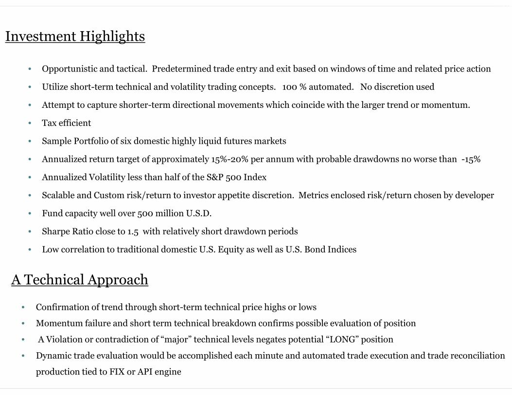
• Opportunistic and tactical. Predetermined trade entry and exit based on windows of time and related price action
• Utilize short-term technical and volatility trading concepts. 100 % automated. No discretion used
• Attempt to capture shorter-term directional movements which coincide with the larger trend or momentum.
• Tax efficient
• Sample Portfolio of six domestic highly liquid futures markets
• Annualized return target of approximately 15%-20% per annum with probable drawdowns no worse than -15%
• Annualized Volatility less than half of the S&P 500 Index
• Scalable and Custom risk/return to investor appetite discretion. Metrics enclosed risk/return chosen by developer
• Fund capacity well over 500 million U.S.D.
• Sharpe Ratio close to 1.5 with relatively short drawdown periods
• Low correlation to traditional domestic U.S. Equity as well as U.S. Bond Indices
A Technical Approach
• Confirmation of trend through short-term technical price highs or lows
• Momentum failure and short term technical breakdown confirms possible evaluation of position
• A Violation or contradiction of “major” technical levels negates potential “LONG” position
• Dynamic trade evaluation would be accomplished each minute and automated trade execution and trade reconciliation
production tied to FIX or API engine

6Portfolio Composition
Monthly and Equally Rebalanced Risk Budget of 6 Futures Markets in Simulation
ES – Mini S&P 500 Index (CME- “Globex”) FV – US Five Year Note (CBOT- “Globex”)
NQ – Mini NASDAQ 100 Index (CME- “Globex) TY – US Ten Year Note (CBOT- “Globex”)
YM - Dow Jones Index (CBOT-”Globex”) US – US 30 Year Bond (CBOT – “Globex”)
0%
10%
20%
30%
40%
50%
60%
70%
80%
90%
100%
15%
20%
25%
30%
2008
1126
2008
1225
2009
0123
2009
0222
2009
0323
2009
0421
2009
0520
2009
0618
2009
0717
2009
0816
2009
0914
2009
1013
2009
1111
2009
1210
2010
0108
2010
0207
2010
0308
2010
0406
2010
0505
2010
0603
2010
0702
2010
0801
2010
0830
2010
0928
2010
1027
2010
1125
2010
1224
2011
0123
2011
0221
2011
0322
2011
0420
2011
0519
2011
0617
2011
0717
2011
0815
2011
0913
2011
1012
2011
1110
2011
1209
2012
0108
2012
0206
2012
0306
2012
0404
2012
0503
2012
0601
2012
0701
2012
0730
2012
0828
2012
0926
2012
1025
2012
1123
2012
1223
2013
0121
2013
0219
2013
0320
2013
0418
2013
0517
2013
0616
2013
0715
2013
0813
2013
0911
2013
1010
2013
1108
2013
1208
20 Day and 200 Day Moving Averages of Margin to Static $1,000,000 PortfolioAugust 2008 to January of 2014
Average Margin to Equity 20.1 %Max Margin to Equity 33.7 %Non-Trading Days of Total Days 16.2 %
0
20
40
60
80
100
120
-6.0
%-5
.9%
-5.7
%-5
.6%
-5.4
%-5
.3%
-5.1
%-5
.0%
-4.8
%-4
.7%
-4.5
%-4
.4%
-4.2
%-4
.1%
-3.9
%-3
.8%
-3.6
%-3
.5%
-3.3
%-3
.2%
-3.0
%-2
.9%
-2.7
%-2
.6%
-2.4
%-2
.3%
-2.1
%-2
.0%
-1.8
%-1
.7%
-1.5
%-1
.4%
-1.2
%-1
.1%
-0.9
%-0
.8%
-0.6
%-0
.5%
-0.3
%-0
.2%
0.0%
0.1%
0.3%
0.5%
0.6%
0.8%
0.9% 1.1%
1.2%
1.4%
1.5%
1.7%
1.8%
2.0%
2.1%
2.3%
2.4%
2.6%
2.7%
2.9%
3.0%
3.2%
3.3%
3.5%
3.6%
3.8%
3.9%
4.1%
4.2%
4.4%
4.5%
4.7%
4.8%
5.0% 5.1%
5.3%
5.4%
5.6%
5.7%
5.9%
6.0%
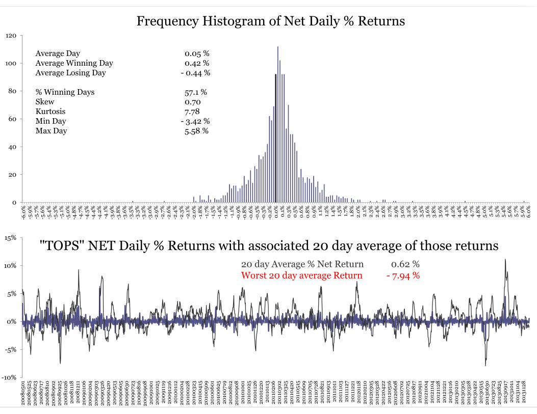
Average Day 0.05 %Average Winning Day 0.42 %Average Losing Day - 0.44 %
% Winning Days 57.1 %Skew 0.70Kurtosis 7.78Min Day - 3.42 %Max Day 5.58 %
Frequency Histogram of Net Daily % Returns
-10%
-5%
0%
5%
10%
15%
2008
0501
2008
0525
2008
0623
2008
0717
2008
0810
2008
0902
2008
0925
2008
1026
2008
1118
2008
1211
2009
0106
2009
0204
2009
0303
2009
0326
2009
0420
2009
0513
2009
0605
2009
0630
2009
0723
2009
0816
2009
0908
2009
1001
2009
1025
2009
1119
2009
1216
2010
0112
2010
0204
2010
0228
2010
0323
2010
0415
2010
0509
2010
0601
2010
0625
2010
0719
2010
0812
2010
0908
2010
1001
2010
1025
2010
1126
2010
1220
2011
0113
2011
0206
2011
0302
2011
0325
2011
0420
2011
0515
2011
0609
2011
0705
2011
0728
2011
0821
2011
0913
2011
1011
2011
1103
2011
1127
2011
1221
2012
0118
2012
0210
2012
0305
2012
0328
2012
0422
2012
0516
2012
0608
2012
0702
2012
0725
2012
0817
2012
0911
2012
1004
2012
1104
2012
1128
2012
1221
2013
0116
2013
0210
2013
0305
2013
0328
2013
0422
2013
0515
2013
0630
2013
0723
2013
0825
2013
0917
2013
1011
2013
1104
2013
1128
"TOPS" NET Daily % Returns with associated 20 day average of those returns20 day Average % Net Return 0.62 %Worst 20 day average Return - 7.94 %

-15.95% -15.64%
-11.72% -11.56%
-9.85% -9.54% -9.15%-8.15%
-6.46% -6.31%
4.12%
0.47%
-2.10%
-4.56%
-0.58%
1.63%2.10%
-0.01%
-3.01%
4.55%
-20%
-15%
-10%
-5%
0%
5%
10%
200811 200810 200902 200901 200809 201005 201205 200806 201109 201108
S&P 500 TOPS
S&P 500 Index worst 10 Months with corresponding "TOPS" SYSTEM Net PerformanceOver the past six years, the average performance of all negative months for S&P 500 Index was -5.83% while "TOPS"
performance average of all negative months over same time period was a mere -1.99 %
S&P 500 average over worst 10 months -10.43 %"TOPS" same period 0.26 %
0
0.5
1
1.5
2
2.5
3
TOPS S&P 500
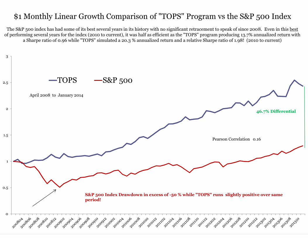
46.7% Differential
Pearson Correlation 0.16
$1 Monthly Linear Growth Comparison of "TOPS" Program vs the S&P 500 IndexThe S&P 500 index has had some of its best several years in its history with no significant retracement to speak of since 2008. Even in this best
of performing several years for the index (2010 to current), it was half as efficient as the "TOPS" program producing 13.7% annualized return witha Sharpe ratio of 0.96 while "TOPS" simulated a 20.3 % annualized return and a relative Sharpe ratio of 1.98! (2010 to current)
S&P 500 Index Drawdown in excess of -50 % while "TOPS" runs slightly positive over sameperiod!
April 2008 to January 2014

10
y = 0.3101xR² = 0.0255
-20%
-10%
0%
10%
20%
-20% -10% 0% 10% 20%
Scattergram Plot of "TOPS" Program Net Monthly Returns vs. S&P 500April 2008 to January 2014
"TOPS" PROGRAM X AXIS
S&P 500 Index Y AXIS

-
0.5
1.0
1.5
2.0
2.5
2008
0409
2008
0512
2008
0613
2008
0716
2008
0818
2008
0919
2008
1022
2008
1124
2008
1228
2009
0130
2009
0304
2009
0406
2009
0510
2009
0611
2009
0714
2009
0816
2009
0917
2009
1020
2009
1122
2009
1224
2010
0128
2010
0302
2010
0404
2010
0506
2010
0608
2010
0711
2010
0812
2010
0914
2010
1017
2010
1118
2010
1221
2011
0124
2011
0225
2011
0330
2011
0503
2011
0605
2011
0707
2011
0809
2011
0911
2011
1013
2011
1115
2011
1218
2012
0124
2012
0226
2012
0329
2012
0501
2012
0603
2012
0705
2012
0807
2012
0909
2012
1011
2012
1113
2012
1216
2013
0120
2013
0221
2013
0326
2013
0429
2013
0531
2013
0703
2013
0805
2013
0906
2013
1009
2013
1111
2013
1213
S&P 500 0.15
US 30 Yr Bond 0.07
Composite Stocks and Bonds 60/40 0.23
TOPS 1.22
Stock/Bond/TOPS Combination 50/30/20 0.46
Growth Profile of Stock and Bond Asset Classes, related Combinationsand risk adjusted by Sharpe Ratio
2008 to 2014

Risk Management and Assumptions
• General information such as net asset value, portfolio composition and risk budgeting are a startingpoint of measuring risk. End of day equal reset of NAV also used on a per million basis per market.This was done to not permit one market to gain or lose too much versus another market which couldsignificantly outperform or underperform.
• Used a $10 per round turn charge per contract as well as $10 per round turn charge for any chargesincurred on spreads from one contract month to the next.
• 1.0 % management fee charged at 1%/12 months. 20% incentive fees charged per month on newportfolio equity highs only. No portfolio risk adjustments were made although this could beaccommodated for managed accounts hoping to produce higher or lower risks.
12
* Parameter selection
One of the biggest challenges in financial engineering; when utilizing simulation constructs to measure future outcomes;is how to avoid fitting the data. The importance of this critical error must be avoided at all cost. Transparency of thecode is one way to reassure some, but even in those situations does the institution validate the concept properly, and notjust its risk attributes?
While constructing "TOPS", much thought was given to these important issues. Based on my own experience in thisindustry, I am keenly aware of the reluctance of financial firms to even consider models presented to them that are basedon simulation, regardless of their merit. Although I don't necessarily disagree with this philosophy, in today's world ofalgorithmic trading; a non-fitted quantitative strategy; that utilizes simple risk/reward rules; that is developed, presentedand understood properly; found to be blindly robust across multiple asset classes should bear some merit. Determininga robustness of signal generation is a science all to itself. It can be very time consuming and to be frank, it is still anassumption that the future will be similar to the past. Trading system evaluation expertise and the related processes usedtoday are scarce and most concentrate on the risk attributes of a particular strategy more than the efficacy of the strategyitself.
(continued)
Engineering & Testing Procedure

13
Parameter Selection Continued:
In the attempt to address any fitting of data and a possible misrepresentation of results, I decided to use a cross sample ofall possible parameters in a population universe defined only by time. (1 to 7 days) I have already described what thegeneral premise that the signal generator looks for…….so the simplicity of the two parameter efficacy of the "TOPS" signalgenerator can also be measured.
The "TOPS" signal generation method looks for targets of opportunities utilizing two parameters. The first parameter isTime/Price(t). Utilizing short-term price action, I began to look at moving TIME/PRICE windows (t’) beginning with aone-day view out to one-week, stepping every 5 hours. That is the complete population of possible selections. As this is ashorter term trading model, to go out further would begin to correlate us to the longer-term market trend so I avoidedgoing out any further than one-week.
The second parameter is Time/Volatility(v) which I call vertical significance or y-axis relevance. Evaluated by (t’) themoving windows of prices, relevant targets of entry and targets of exit are determined by the scalable parameter ofvolatility. So beginning with half or (0.50 * (v’) ) in an associated moving window of time/price and extrapolating out to(1.0 * (v’) ) on the moving time/price window, I documented and averaged all the outcomes.
The multi-parametric results of stepping wide and utilizing *ALL parameter sets as viable trading options are on the nextpage of this brief document. As you can see, there were fluctuations in profitability by shift but overall the trading rulesshow positive results. *ALL of the statistical metrics exhibited in this document are the average of the entireuniverse of tested parameters. Some parameter pairs performed better than others and some worse as is expected.
There are certainly ways to determine which parameter sets overlapped others and muted the overall upside performancebut for the sake of producing a pure signal generation process undeterred by data fitting, *I have used them all.Bootstrapping techniques and Monte-Carlo simulations would also exhibit similar Risk/Return attributes.
* Certainly ALL is relative. Using all selections in the possible universe would produce many thousands of parameter sets and would theoretically produce very similar results towhat is presented here.

$0.8
$1.3
$1.8
$2.3
$2.8
$3.3
2008
0408
2008
0509
2008
0610
2008
0711
2008
0812
2008
0912
2008
1014
2008
1114
2008
1216
2009
0116
2009
0217
2009
0320
2009
0421
2009
0522
2009
0623
2009
0724
2009
0825
2009
0925
2009
1027
2009
1127
2009
1229
2010
0129
2010
0302
2010
0402
2010
0504
2010
0604
2010
0706
2010
0806
2010
0907
2010
1008
2010
1109
2010
1210
2011
0111
2011
0211
2011
0315
2011
0415
2011
0517
2011
0617
2011
0719
2011
0819
2011
0920
2011
1021
2011
1122
2011
1223
2012
0124
2012
0224
2012
0327
2012
0427
2012
0529
2012
0629
2012
0731
2012
0831
2012
1002
2012
1102
2012
1204
2013
0104
2013
0205
2013
0308
2013
0409
2013
0510
2013
0620
2013
0722
2013
0822
2013
0923
2013
1024
2013
1125
2013
1226
30-.5 30-.6 30-.7 30-.8 30-.9 45-0.50 45-0.60
45-0.70 45-0.80 45-0.90 60-0.50 60-0.60 60-0.70 60-0.80
60-0.90 90-0.50 90-0.60 90-0.70 90-0.80 90-0.90 COMPOSITE
Multi-Parameter Growth Simulations – One day to One week time frameApril 2008 to January 2014

1200
1220
1240
1260
1280
1300
1320
2008
0811
2008
0811
2008
0812
2008
0812
2008
0812
2008
0813
2008
0813
2008
0813
2008
0814
2008
0814
2008
0815
2008
0815
2008
0817
2008
0818
2008
0818
2008
0819
2008
0819
2008
0819
2008
0820
2008
0820
2008
0820
2008
0821
2008
0821
2008
0822
2008
0822
2008
0824
2008
0825
2008
0825
2008
0825
2008
0826
2008
0826
2008
0827
2008
0827
2008
0827
2008
0828
2008
0828
2008
0828
2008
0829
2008
0829
2008
0901
2008
0901
2008
0902
2008
0902
2008
0902
2008
0903
2008
0903
2008
0904
2008
0904
2008
0904
2008
0905
2008
0905
2008
0907
2008
0908
2008
0908
2008
0909
2008
0909
2008
0909
2008
0910
2008
0910
"ES" - Mini S&P 500 Monthly Scale Trade Examples60 min chart
Kick out of all possible long positionsmust wait for significant rally from new lows tore-evaluate future entry

1820
1825
1830
1835
1840
1845
1850
1855
1860
1865
1870
2013
1023
2013
1023
2013
1023
2013
1023
2013
1023
2013
1024
2013
1024
2013
1024
2013
1024
2013
1024
2013
1024
2013
1024
2013
1024
2013
1025
2013
1025
2013
1025
2013
1025
2013
1025
2013
1025
2013
1027
2013
1027
2013
1028
2013
1028
2013
1028
2013
1028
2013
1028
2013
1028
2013
1028
2013
1028
2013
1029
2013
1029
2013
1029
2013
1029
2013
1029
2013
1029
2013
1029
2013
1029
2013
1030
2013
1030
2013
1030
2013
1030
2013
1030
2013
1030
2013
1030
2013
1030
2013
1031
2013
1031
2013
1031
2013
1031
2013
1031
2013
1031
2013
1031
2013
1031
"ES" - Mini S&P 500 Detailed Week Trade Examples60 min chart
+ are buys for example chosen parameter- are exits for example chosen parameter
trades are not numbered to match up whichbuy and exit is affiliated
Conclusion
To summarize, the “TOPS” signal generator is a valid and reasonably simple process where neither parameter fitting norany type of learning, walk-forward process is needed to reveal very good results.
This signal generator and basic portfolio was also run over the same six year period on multiple financial instrumentsincluding currencies, metals, commodities, energy and individual stocks with positive and interesting results. Theseadditional tests on other asset classes is always important in my opinion to re-affirm I have NOT fitted a strategy to aspecial circumstance related to just one market.
Trading logic that can exhibit robust positive results across many asset classes is a good indicator that the trading rulesmay have real merit. I also ran these exact trading rules inversely to short markets instead of only buying and exiting.The results were for the most part neutral, but tremendous for those markets which have experienced sustained downcycles in price.
Over the many years of building, reverse engineering and tearing apart trading strategies such as Trend Following,Momentum, Pattern Recognition, Mean Reversion and High Frequency, I can say with confidence that this “TOPS”trading approach is very solid, would be relatively easy to implement and understand and will hopefully be of interest tosomeone looking for a non-correlated strategy with reasonable capacity.
* Further research can be produced as needed for further evaluation.