Comovement of Corporate Bonds and Equities

Jack Bao and Kewei Hou∗

September 23, 2014

Abstract

We study heterogeneity in the comovement of corporate bonds and equities, bothat the bond level and at the firm level. To formalize empirical predictions, we usean extended Merton model to illustrate that, holding the actual maturity constant,corporate bonds that are due late relative to the rest of the bonds in their issuers’maturity structure should have stronger comovement with equities. In contrast, anendogenous default model with equity pay-in suggests that a bond’s position in itsissuer’s maturity structure has little relation with the strength of the comovement.In the data, we find that bonds that are later in their issuers’ maturity structurecomove more strongly with equities, consistent with the prediction of the extendedMerton model. In addition, we find that the comovement between bonds and equitiesis stronger for firms with higher credit risk as proxied by higher book-to-market ratiosand lower distance-to-default even after controlling for ratings. Our results highlightthe important effects of bond and firm level characteristics on the relative returns ofcorporate bonds and equities.

∗Bao is at the Federal Reserve Board of Governors, jack.c.bao@frb.gov. Hou is at the Fisher College ofBusiness, Ohio State University and China Academy of Financial Research (CAFR), hou.28@osu.edu. Wehave benefited from helpful comments from and discussions with Manuel Adelino, Markus Brunnermeier,Sergey Chernenko, Jean Helwege, Jing-zhi Huang, Rainer Jankowitsch, Martin Oehmke, Jun Pan, Eric Pow-ers, Marco Rossi, Ilya Strebulaev, Rene Stulz, Mathijs van Dijk, Yuhang Xing, and Wei Xiong, and seminarand conference participants at Baruch College, BI Norwegian Business School, Boston University, DFA,Erasmus University, Federal Reserve Board of Governors, Inquire UK, INSEAD, Norges Bank InvestmentManagement, North Carolina State University, Ohio State University, Rutgers University, Seoul NationalUniversity, University of Hong Kong, University of Illinois-Chicago, University of South Carolina, TexasA&M University, the 2013 EFA Meetings, and the 2013 South Carolina Fixed Income Conference. Theviews expressed in this paper are those of the authors and do not necessarily reflect the views of the FederalReserve System or its staff. All remaining errors are our own.

1

1 Introduction

Corporate bonds and equities issued by the same firm are different contingent claims on the

same cash flows. The comovement between them has important implications for understand-

ing the relative prices in the two markets as well as for hedging common exposures across

markets. Previous research has found that corporate bonds and equities typically have posi-

tively correlated contemporaneous returns. Furthermore, hedge ratios, the ratio of corporate

bond to equity returns, are larger for bonds with poorer ratings1 and their magnitudes are

in-line with what the Merton (1974) model predicts.2 In this paper we empirically study the

hedge ratios at both the bond level and the firm level to highlight the heterogeneity in the

corporate bond-equity comovement.

We first investigate differences in comovement at the bond level. Most firms issue bonds

at different times with different maturities, providing a rich maturity structure. A bond

that matures after most of the other bonds issued by the same firm is potentially de facto

junior even if they all have the same explicit seniority.3 This arises from the fact that a

firm in financial trouble may remain solvent long enough to repay bonds that are due early

in its maturity structure, but not bonds that are due later. The effect is that bond issues

that mature later are more sensitive to underlying firm value. We formalize this intuition in

an extension of the Merton model and present relative hedge ratios in a numerical exercise

which shows that, holding the actual maturity constant, bonds that are due later in their

firms’ maturity structure have higher hedge ratios.

1See Kwan (1996).2Schaefer and Strebulaev (2008) investigate the Merton model implied hedge ratio within a rating class

and find that they cannot reject the hypothesis that the model implied and empirical hedge ratios are equal.Huang and Shi (2013) confirm this result and reconcile it with the Collin-Dufresne, Goldstein, and Martin(2001) finding that most of the variation in credit spread changes cannot be explained by the Merton model.

3It is important to note that a de facto junior bond is not explicitly junior. While it is straightforwardto extend the Merton model to allow for explicitly junior and senior bonds, it is difficult to empiricallyexamine the effect of explicit seniority on hedge ratios because most corporate bond issues in the UnitedStates are senior unsecured. Furthermore, though bank debt is normally senior to corporate bonds, firmswith significant amounts of corporate bond outstanding often do not have significant bank debt. Rauh andSufi (2010) report that more than 50% of the firms in their sample with significant amounts of corporatebonds have less than 10% of their debt in bank debt. Our sample, which is at the bond-month level, is evenmore extreme, with a median of 2.53% of debt in bank debt.

2

As an alternative to the extended Merton model, we consider the endogenous default

model of Geske (1977), in which equityholders must pay in to retire outstanding bonds

and continue the firm. In this case, the relation between the maturity structure of bonds

and hedge ratios is unclear as equityholders will take the full maturity structure of bonds

into account when making optimal decisions on continuation of the firm, rather than solely

considering the bond due today. Equityholders may choose to default on early bond issues

even if current firm value is much larger than the face value of bonds due early as their

pay-in causes them to take into account the large amount of debt due in the future that will

have to be paid before they receive a payout as residual claimants. In fact, we illustrate that

for reasonable parameter values, the Geske (1977) model predicts that a bond that matures

relatively late in its firm’s maturity structure could have a lower hedge ratio, contrasting

the extended Merton model.4

To empirically test the implications of the two models, we regress corporate bond returns

on equity and Treasury bond returns to calculate empirical hedge ratios. We measure a

bond’s place in its firm’s maturity structure using the proportion of debt due prior to the

bond and interact it with equity returns to determine its effect on the hedge ratio of the

bond. Our primary empirical finding is that, controlling for the actual maturity, bonds that

are due relatively late in their firms’ maturity structure have higher hedge ratios and thus

stronger comovement with equities. For example, if we increase the proportion of debt due

prior for a Baa bond with seven years to maturity from 10% to 80%, its hedge ratio will more

than double from 5.98% to 12.34%. This confirms the prediction of the extended Merton

model and is consistent with de facto seniority affecting corporate bond-equity comovement.

Next, we study firm-level heterogeneity in the comovement between bonds and equities.

Using the standard Merton model, it can be illustrated that firms with greater credit risk

have higher hedge ratios. To the extent that credit ratings capture credit risk well, this should

4We also extend the Geske model to only require equityholders to pay a fraction of the face value of retiringbonds, leaving the remaining portion to be paid from firm value. Except for cases where equityholders’ pay-inis very small, the empirical predictions of this extension are very similar to the Geske model.

3

be reflected in higher average hedge ratios for poorer credit ratings. More importantly, if the

market is able to distinguish between the credit quality of bonds issued by firms with similar

credit ratings, we should see significant within-rating variation in hedge ratios.5 Using book-

to-market ratio, a reduced form measure of credit risk, and distance-to-default, a structural

model-based measure of credit worthiness, we examine whether the comovement of corporate

bonds and equities is related to market perceptions of credit risk that are finer than credit

ratings. We find that this is indeed the case, as high book-to-market and low distance-to-

default firms (firms that are perceived as having higher credit risk) have stronger comovement

between bonds and equities within ratings. For example, a one standard deviation increase

in book-to-market ratio (distance-to-default) above the mean is associated with an increase

(decrease) in the hedge ratio for a seven-year Baa bond from 7% to 9.52% (from 6.94% to

3.87%). These effects are comparable in magnitude to the effect of credit ratings on hedge

ratios. The results for distance-to-default are particularly telling as the measure is based

on the Merton model. Even a simple structural model of default that incorporates only

asset volatility and leverage provides significant information above and beyond ratings. Our

results suggest that at least in the corporate bond market, market participants recognize

more granular differences in credit risk than what is provided by ratings, and this is reflected

in the joint dynamics of corporate bond and equity returns.

Our paper is primarily related to three strands of literature. At the most fundamental

level, our paper is related to the literature that tries to empirically evaluate the pricing

of corporate bonds through the lens of structural models of default. Huang and Huang

(2003) is the seminal paper, showing that a large part of credit spreads cannot be explained

by structural models of default. In contrast, Schaefer and Strebulaev (2008) argue that

even a first generation model like the Merton model can reasonably characterize the average

magnitude of hedge ratios. Bao and Pan (2013) find that the corporate bond market is

excessively volatile compared to equities when a Merton model is used, but attribute this

5However, the recent subprime mortgage crisis has cast doubt on the quality of credit ratings and suggestedthat market participants have relied too heavily on ratings.

4

largely to illiquidity in the corporate bond market.6

Our focus on the maturity structure of bonds is most closely related to the theoretical

work of Brunnermeier and Oehmke (2013) and Chen, Xu, and Yang (2012) who construct

equilibrium models of maturity choice. The primary contribution in Brunnermeier and

Oehmke (2013) is in using the intuition of de facto seniority to show that in equilibrium,

financing is inefficiently short-term. Chen, Xu, and Yang (2012) instead consider the interac-

tion between rollover and systematic risk, finding that firms with more systematic volatility

will choose longer bond maturities. In our paper, we do not aim to explain why a firm has

chosen a particular maturity structure, instead taking the outcome of maturity choice as

given and focusing on the empirical effects of maturity structure outcomes on the observed

comovement between corporate bonds and equities. Importantly, we note that our results

are robust to controlling for the average firm-level maturity (the outcome of the endogenous

choices discussed in the aforementioned papers) and also the actual maturity of the bond.

Furthermore, corporate bond issuers will always have both de facto senior and de facto ju-

nior bonds regardless of the equilibrium choice to largely issue short-term versus long-term

bonds as de facto priority is defined relative to bonds from the same issuer, not based on

the absolute maturity of the bond.

Finally, our paper is related to the recent literature that examines how dependent the

market is on credit ratings. In the context of MBS, Adelino (2009) finds that the market

was unable to distinguish between different Aaa-rated securities, but was able to distinguish

between different securities within lower rating groups. As the vast majority of MBS are

Aaa-rated, this suggests a heavy dependence by the market on ratings. In contrast, our

results suggest that at least for corporate bonds, the market is capable of evaluating credit

quality at a finer level and does not naively rely on credit ratings.

6We note that there is an extensive literature focusing on the comovement between Treasury bonds andequities. Recent papers include Baele, Bekaert, and Inghelbrech (2010), Baker and Wurgler (2012), andCampbell, Pflueger, and Viciera (2013). In addition, there is a literature that examines bond and equityreturns over corporate announcement windows, including Hotchkiss and Ronen (2002), Maxwell and Stephens(2003), and Maxwell and Rao (2003).

5

The rest of the paper is organized as follows. In Section 2, we formalize empirical predic-

tions for hedge ratios by using structural models of default. In Section 3, we discuss the data,

summary statistics, and the construction of some key variables. In Section 4, we discuss our

empirical results. We conclude in Section 5.

2 Credit Risk and Hedge Ratios

The theoretical relation between corporate bond and equity returns is formalized in structural

models of default, the earliest of which is the Merton (1974) model. Structural models posit

processes for firm value and other state variables and all securities that are claims on the firm

can be priced from these processes. This ties corporate bonds and equities together through

their sensitivities to state variables and provides important intuition as to why their returns

should be related. Though Huang and Huang (2003) find that structural models of default,

when calibrated using historical default rates and the equity premium, perform quite poorly

in explaining the levels of corporate bond prices, Schaefer and Strebulaev (2008) find that

even a structural model as simple as the Merton model does well in characterizing the average

relative returns of corporate bonds and equities. This points to trying to understand relative

returns rather than relative prices as the more promising direction to explore structural

models.7

2.1 Merton Model

In the Merton model, the only state variable is the value of the firm, which is assumed to

follow a Geometric Brownian Motion under the risk-neutral probability measure

d lnVt =

(r − 1

2σ2v

)dt+ σvdW

Qt . (1)

7Note that many structural models including the Merton model do not take a stand as to what the correctpricing kernel is. Instead, they are based on no arbitrage and the consistent pricing of different securities.

6

The firm has a single zero-coupon bond issue with face value K and equity is a call option

on the firm. The single bond issue is equivalent to a risk-free bond short a put option on

the firm. Its value is

B = V (1−N(d1)) +Ke−rTN(d2), (2)

where d1 =ln(VK

)+(r + 1

2σ2v

)T

σv√T

, d2 = d1 − σv√T .

As illustrated by Schaefer and Strebulaev (2008), the relative returns of the bond and equity

(the hedge ratio) under the Merton model is

hE ≡∂ lnB

∂ lnE=

(1

N(d1)− 1

)(V

B− 1

). (3)

The Merton model formalizes the important insight that corporate bonds and equities

are linked through their exposures to the underlying firm value.8 Furthermore, the Merton

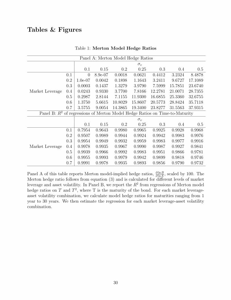
model-implied hedge ratio is increasing in both asset volatility and leverage as higher asset

volatility and leverage are associated with greater likelihood of default. To see this, in

Panel A of Table 1, we report Merton model-implied hedge ratios for various leverage-asset

volatility combinations.9 The reported hedge ratios bear out the intuition that bonds issued

by safer firms have lower hedge ratios. For a firm with a market leverage of 10% and

asset volatility of 20%, the model hedge ratio is 0.0018%. That is, a 10% equity return

corresponds to only a 0.00018% corporate bond return, an economically insignificant return.

Such a small relative return for the corporate bond reflects the fact that at 10% leverage

and 20% asset volatility, the likelihood of default is extremely low. As a result, the bond has

similar dynamics as a risk-free bond and its returns are essentially unrelated to the returns

8Note that an important source of variation in bond prices, stochastic interest rates, is not modeled hereas the tie between bonds and equities through interest rates is indirect and less important than the tiethrough firm value. See Shimko, Tejima, and van Deventer (1993) for an extension of the Merton model tostochastic interest rates and Schaefer and Strebulaev (2008) and Bao and Pan (2013) for applications of thismodel.

9The maturity T is set to seven years to be in line with the average remaining maturity of outstandingU.S. corporate bonds.

7

of equity. In contrast, the relative returns of corporate bonds to equities are much more

important at higher leverages and asset volatility. For example, at 70% market leverage and

20% asset volatility, the hedge ratio is 14.39%. Thus, a 10% equity return corresponds to a

1.439% bond return. Or consider 10% market leverage and 50% asset volatility; the hedge

ratio is 8.49%, which means a 10% equity return is associated with a 0.849% bond return.

Finally, at 70% market leverage and 50% asset volatility, the hedge ratio is 37.93%. In this

case, a 10% equity return is associated with close to 4% bond return. The effects of leverage

and asset volatility on hedge ratios can also be seen in Figure 1(a) where we plot the Merton

model-implied hedge ratios against market leverage and asset volatility.

It is clear from the Merton model that as firms become more risky in the dimensions

of leverage and asset volatility, hedge ratios become larger. Ratings are widely used by

academic researchers and investment professionals as an aggregate measure of credit risk

and have proved to be very useful. However, they are also a coarse measure. Based on the

preceding analysis of credit quality and hedge ratios in the Merton model, we would expect

more granular measures to be able to predict within-rating variation in hedge ratios if the

measures are credible and the market is able to understand the information that they provide

above and beyond ratings.

2.2 Extending the Merton Model

A number of authors have derived extensions of the Merton model that involve changing the

underlying state variables, state variable processes, default triggers, and capital structure.10

Here we focus our attention on the capital structure. The simplest extension to the capital

structure in the Merton model is to allow for both junior and senior bonds.11 Such an

extension is straightforward. Equity and the senior bond are priced in the same way as in

the standard Merton model, but the junior bond is the difference between two call options.

10For example, see Black and Cox (1976), Leland (1994), Longstaff and Schwartz (1995), Leland and Toft(1996), Collin-Dufresne and Goldstein (2001), Duffie and Lando (2001), Chen, Collin-Dufresne, and Golstein(2009), and Collin-Dufresne, Goldstein, and Helwege (2010), among others.

11See Black and Cox (1976) and Lando (2004). We also provide further discussion in Appendix A.

8

If the recovery rate in default states is sufficiently high, the senior bond is very safe and

has dynamics that are similar to a risk-free bond; the junior bond, which bears the first

loss, is riskier and has a higher hedge ratio than the senior bond. However, as discussed in

the introduction of this paper, this is difficult to examine empirically due to the paucity of

significant explicit seniority structure among corporate bonds.

Our extension is similarly based on having multiple bond issues, but in the dimension

of the maturity structure of the firm. We analyze how the position of a bond in a firm’s

maturity structure affects its hedge ratio. As discussed by Brunnermeier and Oehmke (2013),

shorter maturity bonds may be de facto senior to longer maturity bonds. The intuition is

that a firm that is in financial distress may remain solvent long enough to repay bond issues

that mature early. However, the firm is then likely to suffer solvency issues when the bonds

due later eventually mature.

To formally analyze the effect of maturity structure, we extend the Merton model to

include three zero-coupon bond issues, which have the same explicit seniority, but mature

at different times. The three bond issues have face values Ki and maturities Ti where

T1 < T2 < T3. At Ti, a firm remains solvent if Vi > Ki. Otherwise the firm defaults, Vi is

discounted by a proportional bankruptcy cost (L), and the remaining bond issues share the

remaining firm value in proportion to their face values.12

This model, while a simplification of the complex capital structure typical in large U.S.

corporations, allows us to examine the sensitivity of a firm’s bond returns to its equity

returns while varying the bond’s position in the firm’s maturity structure. By including

three bonds, we are able to focus on the bond with the intermediate maturity, T2, and

adjust the relative amounts of debt due before and after it.13 This changes the de facto

12We do not formally model the decision to rollover debt, but the states where Vi is barely larger thanKi are the states where the rollover of debt would be particularly expensive, if not impossible. These arealso the states that are primarily responsible for driving the wedge between bond issues that creates de factoseniority. See He and Xiong (2012) and He and Milbradt (2013) for recent papers that examine the issue ofrollover risk.

13Our set-up essentially maps all bonds maturing prior to T2 into a single bond that matures at T1 andall bonds maturing after T2 into a single bond that matures at T3.

9

seniority of the intermediate maturity bond, holding all else constant, allowing us to gauge

the impact of de facto seniority on hedge ratios.

In this extended Merton model, equity remains a call option on the firm, but has inter-

mediate monitoring points at each bond maturity

E = EQ0

[e−rT31V1>K11V2>K21V3>K3 (V3 −K3)

]. (4)

Though there is no closed-form solution for equity value, it can be simplified to a function of

normal CDFs and integrals by noting that firm value returns are lognormal. Similarly, the

value of the bond maturing at T2 is

B = EQ0

[e−rT21V1>K11V2>K2K2

]+ EQ

0

[e−rT11V1<K1(1− L)V1

K2

K1 +K2 +K3

](5)

+ EQ0

[e−rT21V1>K11V2<K2(1− L)V2

K2

K2 +K3

],

where the three terms represent solvency at T2, default at T1, and default at T2, respectively.

The hedge ratio(∂ lnB∂ lnE

)can then be calculated using numerical procedures. See Appendix

B for further details.

To examine the implications of the extended Merton model, we consider two scenarios.

In both scenarios, we fix the value of the bond due at T2 to be 10% of the total market value

of debt. In the first scenario, 80% of the firm’s market value of debt is from the bond due at

T3 and only 10% of the market value of debt is from the bond due at T1. In this scenario,

the intermediate maturity bond, due at T2, is de facto senior to most of the debt in the firm.

In the second scenario, we flip the proportions of the market value of debt due to the bonds

maturing at T1 and T3, making the intermediate maturity bond de facto junior to most of

the firm’s debt. We set the risk-free rate to be 3%, the maturities of the three bonds to be

T1 = 5, T2 = 7, and T3 = 10, and the bankruptcy cost to be L = 0.5. We present the hedge

ratios of the intermediate maturity bond for the two scenarios in Table 2 and also plot them

10

in Figure 1(b).

Table 2 and Figure 1(b) show that the hedge ratio for the intermediate maturity bond is

higher when the bond is de facto junior (a larger proportion of the firm’s debt is due prior

to the bond) than when it is de facto senior, especially for firms with significant leverage

and/or asset volatility. For example, a bond that is de facto senior has a hedge ratio of

0.0048% when the firm has a market leverage of 70% and an asset volatility of 20%. This

is an economically very small hedge ratio as it implies that a 10% equity return is only

associated with a 0.00048% bond return. This is despite the fact that the firm has very

high leverage. In contrast, when the bond is de facto junior, the hedge ratio is substantially

higher at 26.52%. A 10% equity return now corresponds to a 2.652% bond return. The

intuition follows from the sequential repayment of debt. If a firm is in financial distress, it

may still be able to repay the principal on bonds that mature early in the firm’s maturity

structure. It is much less likely that the firm will be able to remain solvent long enough to

repay the principal on the bonds that are late in the firm’s maturity structure. Thus, bonds

that are early in a firm’s maturity structure (de facto senior) can be very safe even if the firm

itself is in some financial distress. These bonds will have little sensitivity to the underlying

firm value, the main tie between corporate bonds and equities. Bonds that are late in the

maturity structure of a risky firm will be particularly risky, and consequently, have stronger

comovement with equities.

We can also compare the hedge ratios of de facto senior and de facto junior bonds to

the original Merton case with no maturity structure. For the case of 70% market leverage

and 20% asset volatility discussed above, the Merton model hedge ratio reported in Table

1 is 14.39%, which is significantly higher than the de facto senior hedge ratio of 0.0048%

but is considerably lower than the de facto junior hedge ratio of 26.52%. A comparison of

other market leverage-asset volatility combinations between Tables 1 and 2 shows a similar

pattern. For most cases, the hedge ratio given by the Merton model falls between the hedge

ratios of de facto senior and de facto junior bonds. This suggests that if de facto seniority is

11

not taken into account, the Merton model will produce model-implied hedge ratios that are

too high for bonds that mature early in a firm’s maturity structure and too low for bonds

that mature late in the firm’s maturity structure.

2.3 Geske Model

The extended Merton model in Section 2.2 is based on the assumption that upon bond

maturity, the face value of the bond is paid out of the value of the firm. There is no explicit

choice for equityholders to make (though given the choice, they would always choose to

continue the firm as the value of their residual claim if the firm defaults is zero). Another class

of structural models of default, endogenous default models, force equityholders to directly

bear the cost of payouts (either coupons, face value payments, or both) to bondholders.14

Thus, at each moment that there is a payoff, equityholders make an decision by trading-off

the value they must pay to continue the firm against their claim to the value of the firm as

a going concern. This pay-in induces equityholders to consider the full maturity structure

of the firm when deciding whether to continue the firm.

Here, we consider the Geske (1977) model.15 In the Geske model, as in most structural

models of default, equityholders are residual claimants of the firm. That is, if the firm

survives to the very last promised payment to bondholders at time T , equityholders receive

max(0, VT−KT ), where VT is the value of the firm at T and KT is the last promised payment.

At any prior time t with a payment to bondholders of Kt, equityholders must decide whether

to pay Kt and allow the firm to continue or to force the firm to default and put the firm to

bondholders. Effectively, equityholders are making an optimal decision based on the market

value of max(0, VT −KT ) at t compared to the payment Kt.

Similar to our extension of the Merton model, we include three zero coupon bonds with

14Masulis and Korwar (1986) find that in a sample of 1,406 announcements of stock offerings, 372 of-ferings are planned exclusively to refund outstanding debt. This suggests that there is a realistic role forequityholders in paying off debt.

15See also Leland (1994) and Leland and Toft (1996) for models that incorporate optimal decisions byequityholders. Similar to the Geske (1977) model, in these models, equityholders optimally choose whetheror not to service debt.

12

maturities T1 < T2 < T3 and focus on the intermediate maturity bond while varying the

proportion of the firm’s debt value due to the first and third bonds. We again consider

two scenarios, the first where the bond maturing at T3 accounts for 80% of the firm’s debt

value and the second where the bond maturing at T1 accounts for 80% of the firm’s debt

value. This allows us to compare the case where most of the firm’s debt is due after the

intermediate maturity bond and the case where most of the firm’s debt is due before the

intermediate maturity bond.

Rather than providing the full set of Geske pricing formulas for general cases, we instead

focus on the intuition of the Geske model under the special case that we implement, which

is best understood through a recursive framework. In the Geske model, firm value follows a

Geometric Brownian motion as in the Merton model. Also as in the Merton model, if the

firm survives until there is only one bond outstanding (the bond with maturity T3 in our

example), equity is a residual claim and receives a payoff of max(0, V3 −K3) at T3.

Consider the value of equity and the long maturity bond at T2 and suppose that equi-

tyholders have just decided to pay the face value of the intermediate maturity bond, K2,

to continue the firm. This becomes the standard Merton model as equityholders have no

remaining decisions to make. The value of equity is now

E2 = V2N(d1)−K3e−r(T3−T2)N(d2), (6)

d1 =ln(V2K3

)+(r + 1

2σ2v

)(T3 − T2)

σv√T3 − T2

, d2 = d1 − σv√T3 − T2.

That is, equity is a call option on the firm and the long maturity bond is a risk-free bond

short a put option on the firm.

We can now consider the optimal decision of equityholders at T2. The decision that

equityholders make is simple. If the value of equity given in equation (6) is greater than K2,

they pay K2 and continue the firm. Otherwise, equityholders force the firm to go bankrupt.

Even if K2 is small, equityholders may still choose bankruptcy because K3 is very large.

13

Equityholders’ decision at T1 is similar, though the trade-off that equityholders make is

between the payment of the face value of the short maturity bond, K1, and the value of

equity as a going concern which is a compound call option. Because equityholders take into

account the full maturity structure of the firm’s debt, even bonds that mature relatively

early can have significant exposure to underlying firm value. Intuitively, even if the debt due

early has a low face value, equityholders know that they will only receive a non-zero payoff

in the future if the firm value is high enough to cover all face value payments in the future.

Having large face values due in the future would be equivalent to buying an out-of-the-money

call option, so even a small pay-in may induce default.

As noted by Eom, Helwege, and Huang (2004), the Geske formula is not straightforward

to implement accurately, particularly for long maturity bonds. Thus, we follow Huang (1997)

and Eom, Helwege, and Huang (2004) and implement the Geske model using a Cox, Ross, and

Rubinstein (1979) binomial tree, and the equity and bond values, as well as the hedge ratio,

are determined numerically. We also verify the accuracy of this numerical implementation

by running simulations.

Table 3 and Figure 1(c) present the hedge ratios for the intermediate maturity bond for

the scenarios where (1) most of the debt is due after the intermediate maturity bond and (2)

most of the debt is due prior to the intermediate maturity bond. Recall that for the extended

Merton model, the hedge ratio is generally lower in the first scenario. The intuition follows

from the fact that if most of the debt is due after T2, the firm would very likely have enough

value to pay bondholders at T2 directly from firm value. Thus, the intermediate bond has

little sensitivity to firm value and consequently a low hedge ratio. In the Geske model, the

intuition is less clear. Even if most of the firm’s debt is due at T3, equityholders may still

choose to default at T2 as their payoff at T3 contingent on continuation, max(0, V3 − K3),

may have a low expected value due to the large amount of debt due at T3. In fact, we

find that for the same set of parameters as the extended Merton model, the Geske model

generates slightly lower hedge ratios for scenario 2 than scenario 1 for almost all leverage-

14

asset volatility combinations.16 For example, consider again the firm with a 70% market

leverage and a 20% asset volatility; the Geske model produces a hedge ratio of 30.43% for

the intermediate maturity bond for scenario 1 versus a hedge ratio of 27.79% for scenario 2.

Thus, a 10% equity return is associated with a 3.043% return for the intermediate maturity

bond when most debt is due after the bond compared to a 2.779% return when most debt is

due before the bond. These results contrast with the extended Merton model which predicts

a hedge ratio of 0.0048% for scenario 1 and 26.52% for scenario 2. This contrast between

the extended Merton model and Geske model can clearly be seen in Figure 1(d) which shows

that the difference in hedge ratios is close to 0 for the Geske model whereas the difference

in hedge ratios is economically significant for the extended Merton model.

In Appendix C, we consider an extension of the Geske model which allows for a fraction

α of maturing debt to be paid out of firm value rather than by equityholders. The standard

Geske model corresponds to the case where α = 0, whereas the extended Merton model

corresponds to the case where α = 1. As described in more detail in the Appendix, low to

moderate values of α generate little difference between the hedge ratios of the intermediate

bond when most of the firm’s debt is due after the bond (scenario 1) and when most the

firm’s debt is due before the bond (scenario 2). It is not until α is close to 1 where we begin

to see a significant difference in hedge ratios between the two scenarios.17

2.4 Other Measures of Credit Risk

In the standard Merton model, credit risk is a function of leverage and asset volatility. As

illustrated earlier in Table 1, hedge ratios increase with both leverage and asset volatility.

The intuition follows from the fact that as credit risk increases, the value of bonds become

16The slightly lower hedge ratios for the case where the bond is relatively late in the maturity structure isattributable to the fact that we model bonds as zero coupon bonds and the recovery as being in proportionto the face value. Thus, bonds late in the maturity structure receive a slightly disproportionate recoveryrelative to market values.

17To the extent that managers are not perfectly aligned with equityholders and internalize the cost ofeffort in continuing a firm, a small required equity pay-in can also be conceptually thought of as requiredmanagerial effort rather than an explicit stock issuance to refund outstanding debt.

15

more sensitive to the underlying firm value. Indeed, both Kwan (1996) and Schaefer and

Strebulaev (2008) find that empirical hedge ratios are larger as ratings decline. Ratings,

however, are both coarse and slowly updated measures of credit risk. If market participants

are able to assess credit quality at a more granular level than ratings, we would expect to

see larger hedge ratios for firms with greater credit risk within ratings.

On the other hand, recent evidence from the MBS market suggests that it is unclear

whether the market makes its own assessment of credit quality above and beyond what is

provided by credit ratings. Adelino (2009) finds evidence that yield spreads at issuance do

not predict future downgrades and defaults within Aaa-rated MBS, but do predict future

downgrades and defaults for all other ratings. As Aaa-rated MBS constitute roughly 90% of

MBS issuance, this suggests that the vast majority of the MBS market do rely heavily on

ratings.

We consider two other measures of credit risk that have been used extensively in the

academic literature and are also prominent in credit risk assessment in practice, book-to-

market ratio and distance-to-default. Book-to-market ratio, the ratio of the book value of

equity to the market value of equity, is a reduced form proxy of a firm’s default likelihood

and has been found to be related to the relative strength of a firm’s economic fundamentals

(Lakonishok, Shleifer, and Vishny (1994) and Fama and French (1995)). Though there is

much debate as to whether the equity return premium associated with book-to-market ratio

is due to risk or mispricing (see e.g., Fama and French (1993, 1996), Lakonishok, Shleifer,

and Vishny (1994), Haugen (1995), MacKinlay (1995), and Daniel and Titman (1997)), our

use of the book-to-market ratio is much more basic. We simply take it as a indicator of the

market’s assessment of the default prospects of a firm.

Distance-to-default is a structural-based proxy for default risk that is predicated on the

Merton model. It is widely used in both the academic literature (e.g., Hillegeist, Keating,

Cram, and Lundstedt (2004), Vassalou and Xing (2004), Campbell, Hilscher, and Szilagyi

(2008), and Bharath and Shumway (2008)) and credit assessment practice (e.g., KMV) to

16

measure how far a firm is from its default boundary.18

3 Data and Summary Statistics

3.1 Data

The corporate bond dataset used in this paper is the Financial Industry Regulatory Author-

ity’s (FINRA) TRACE. This dataset is the result of a regulatory initiative to increase price

transparency in the corporate bond market and was implemented in three phases. On July 1,

2002, the first phase was implemented, requiring transaction information to be disseminated

for investment grade bonds with an issue size of $1 billion or greater and 50 legacy high-

yield bonds from the Fixed Income Pricing System (FIPS). Approximately 520 bonds were

included in Phase I. Phase II, which was fully implemented on April 14, 2003, increased

the coverage to approximately 4,650 bonds and included smaller investment grade issues.

Phase III, which was fully implemented on February 7, 2005, covered approximately 99% of

secondary bond market transactions. In 2010, FINRA added coverage of U.S. Agency bonds

and in 2011, asset-backed and mortgage-backed securities. In our study, we use TRACE

data on corporate bonds from July 2002 to December 2010.

Bond transaction data from TRACE is merged with bond characteristics data from Mer-

gent FISD, which allows us to determine bond characteristics such as age, maturity, amount

outstanding, and rating. This data is then merged with equity return data from CRSP and

accounting information from Compustat. Treasury data is obtained from the Constant Ma-

turity Treasury (CMT) series. Mergent FISD is used to eliminate bonds that are putable,

convertible, or have a fixed-price call option.19 CRSP is used to eliminate bonds issued by

18KMV, which was acquired by Moody’s in 2002, uses distance-to-default to assess expected defaultfrequency (EDF). See Crosbie and Bohn (2003). Though Moody’s puts out both credit ratings and EDFs,EDFs are not used explicitly in assigning ratings. Moody’s publishes guides for their ratings methodologiesby industry. The four broad criteria that are typically used are scale and diversification, profitability, leverageand coverage, and financial policy. If a firm has an explicit seniority structure, Moody’s will then notch thebonds. Secured bonds receive a one notch upgrade from senior unsecured bonds and subordinated bondsreceive a one notch downgrade.

19Bonds where the only provision is a make whole call provision, which constitutes a significant portion of

17

financial firms.20

3.2 Bond Returns and Summary Statistics

While equity returns can be directly obtained from CRSP, both corporate bond and Treasury

returns need to be calculated. To calculate monthly corporate bond returns, we use the last

trade for a bond in a month and calculate log returns as

rt+1 = ln

(Pt+1 + AIt+1 + Ct+1

Pt + AIt

), (7)

where Pt+1 is the clean price, AIt+1 is the accrued interest, and Ct+1 is the coupon paid

during the month (if applicable).21

Unlike equities, many corporate bonds do not trade every day. Thus, the returns that we

calculate for a bond in a particular month may not necessarily be based exactly on month-

end to month-end prices. To account for this, we make two adjustments. First, we match

Treasury and equity returns to the exact dates that are used to calculate bond returns. This

eliminates any issues of non-synchronization as our goal is to compare contemporaneous

bond, equity, and Treasury returns. Second, we scale all log returns to make them monthly.

For example, if a log bond return is calculated over 25 business days, we scale the return by

2125

to make it comparable to a return that actually occurs over exactly a one month period

(≈ 21 business days).

An additional complication that arises in calculating corporate bond returns is the severe

non-financial bonds, are kept. Make whole calls involve redemption at the maximum of par and the presentvalue of all future cash flows using a discount rate of a comparable Treasury plus X basis points, wherethe most common values of X are 20, 25, and 50. Historically, the average AAA yield spread has beengreater than 50 basis points, leaving make whole calls with little chance of being in-the-money. Powers andTsyplakov (2008) show that theoretically, make whole calls have little effect on bond prices. They also findthat by 2002-2004, the empirical effect of make whole calls on bond prices is extremely small.

20Though some corporate bond studies, primarily those on corporate bond illiquidity, retain financialfirms, studies on structural models of default typically drop financial firms due to different implications ofleverage for financial firms. Furthermore, Brunnermeier and Oehmke (2013) argue that financial firms areunable to commit to a maturity structure. Thus, any measure of maturity structure today for a financialfirm is unlikely to reflect bondholders’ expectations of future maturity structure.

21We apply standard filters for corrected and canceled trades and eliminate obvious errors.

18

illiquidity of the corporate bond market. This illiquidity creates two potential problems in

our analysis. First, by using transaction prices, returns can be non-zero simply because a

trade at bid follows a trade at ask or vice versa.22 As shown in Edwards, Harris, and Piwowar

(2007) and Bao, Pan, and Wang (2011), the effective bid-ask spreads of corporate bonds are

very large. This introduces additional noise in our measurement of bond returns, making

it more difficult to find statistically significant results. However, it should not bias point

estimates as long as bond returns are used as the regressor.23

A second potential concern is that illiquidity is priced in the corporate bond market. The

past literature has found a significant relation between yield spreads and different proxies

for illiquidity.24 Thus, we might expect that the average level of corporate bond returns is

positively related to illiquidity and that some of the variation in bond returns is explained

by changes in illiquidity. However, there does not appear to be a clear ex-ante theoretical

reason for illiquidity to affect the hedge ratio. Therefore, we do not make an adjustment for

illiquidity in the results reported in the paper. Nevertheless, we also re-run our main tests

to allow for both the level of returns and hedge ratios to vary with bond illiquidity and find

that our primary conclusions remain unchanged.

To calculate Treasury returns, we use yields from the U.S. Department of Treasury’s

Constant Maturity Treasury (CMT) series. The provided yields are par yields for on-the-

run (and hence, liquid) bonds. Because the yields are par yields, we can calculate the return

for a bond that trades at par at the start of a month by discounting cash flows using yields

at the end of the month. Only discrete maturities are provided in the CMT series. Thus, we

interpolate between maturities to calculate the return for a Treasury with the same maturity

22One way to address this issue would be to average prices over the last few days of the month to obtainprices where the bid-ask spread is (partially) washed out by averaging over a number of trades at both bidand ask. However, this creates a mismatch between the timing of corporate bond returns and that of equityand Treasury returns as corporate bond prices would be an average over multiple days.

23Indeed, both Kwan (1996) and Schaefer and Strebulaev (2008) regress bond returns on equity returnsrather than equity returns on bond returns to avoid the attenuation bias arising from imprecisely measuredregressors.

24See Chen, Lesmond, and Wei (2007), Bao, Pan, and Wang (2011), and Dick-Nielsen, Feldhutter, andLando (2012), among others.

19

as the corporate bond being studied.

Table 4 reports summary statistics for our corporate bond sample. The majority of the

sample are rated A or Baa by Moody’s, with these ratings covering 73.5% of the bond-months

of the sample. Across ratings, the average time-to-maturity ranges from 6.8 to 9.5 years and

the average age from 4.5 to 6.3 years. To measure a bond’s position in its firm’s maturity

structure, we calculate the proportion of the firm’s total face value of current outstanding

debt from FISD that has a shorter remaining maturity than the bond being studied. Note

that this includes all debt in Mergent FISD, not just bonds traded in TRACE. Its average

value varies from 33% to 50% across ratings. On the dimensions of amount outstanding,

coupons, and yield spreads, we observe more systematic differences across ratings. Poorer

rated bonds tend to have smaller amount outstanding, higher coupon rates, and higher yield

spreads. The smaller amounts outstanding reflect the fact that firms with poorer ratings

tend to be smaller and the higher coupon rates reflect the fact that most corporate bonds

are issued at par. The average yield spread for our Aaa & Aa sample is 113 basis points

compared to 573 basis points for B. There is also a large jump at the investment grade/junk

cut-off as Baa bonds have an average yield spread of 217 basis points compared to 426 basis

points for Ba.

In comparison to yield spreads, the log realized returns for bonds in our sample show a

less pronounced relation with ratings. This can be attributed primarily to two reasons. First,

realized bond returns for a period of 8.5 years do not necessarily reflect ex-ante expected

returns.25 Second, while yield spreads may be monotonically increasing as ratings become

poorer, this is not necessarily the case for expected returns. Yield spreads are promised

returns and reflect both expected returns and the probability of default. As the probability

of default has historically been higher for bonds of poorer ratings, we would expect to see

higher yield spreads for poorer ratings even if expected returns do not vary across ratings.

25As shown in Hou and van Dijk (2012), conclusions can vastly differ when ex-ante expected returns areused rather than ex-post realized returns in asset pricing tests.

20

3.3 Other Default Proxies and Firm Summary Statistics

We construct the book-to-market ratio (B/M) in a similar manner to Asness and Frazzini

(2011), who argue that it is important to use more timely stock price data relative to book

data in order to better forecast future book-to-market ratio.26 For the book value of equity,

we use the book value of common equity (CEQ) from Compustat and assume that it is

publicly available three months after the fiscal year end. For the market value of equity, we

use common shares outstanding (CSHO) times price at the end of the fiscal year (PRCC F),

but adjust this using returns without dividends from CRSP. For example, to calculate the

B/M ratio for a firm in May 2010 whose last fiscal year ended in December 2009, we take

the book equity and market equity (CSHO × PRCC F) from Compustat at the end of the

2009 fiscal year and scale the market equity by (1 + r) where r is the return of the firm’s

equity without dividends from December 2009 to May 2010.27

Table 5 shows that firms with poorer ratings tend to have higher B/M ratios. The average

B/M for bonds rated Aaa & Aa and A are 0.39 and 0.41, respectively. In comparison, the

average B/M are 0.61, 0.91, and 0.79 for Baa, Ba, and B-rated bonds, respectively. This is

consistent with the notion that high B/M is associated with relative distress.

Following Campbell, Hilscher, and Szilagyi (2008), we calculate the distance-to-default

as

DD =ln(VK

)+ 0.06 + rf − 1

2σ2v

σv. (8)

As in the previous literature, we measure K as debt in current liabilities (DLC) plus one-half

times long-term debt (DLTT). The primary complication that arises in solving for DD is that

the firm value, V, and asset volatility, σv, are unobservable. As in Hillegeist, Keating, Cram,

26This is particularly critical for our purposes as one of the drawbacks to using credit ratings in creditassessment is that they are updated infrequently.

27Directly using market equity from CRSP for May 2010 introduces errors if the firm had significantissuance or repurchases between December 2009 and May 2010 which would be reflected in the marketequity for May 2010, but not in the book equity for December 2009.

21

and Lundstedt (2004) and Campbell, Hilscher, and Szilagyi (2008), we solve for V and σv

by simultaneously solving the Merton model equation for equity value and equity volatility

E = V N(d1)−Ke−rTN(d2), (9)

and

σE = N(d1)V

Eσv. (10)

Table 5 reports the average distance-to-default estimates, which decrease monotonically

from a high of 10.24 for Aaa & Aa bonds to a low of 4.55 for B bonds. Since differences in

distance-to-default should reflect differences across firms in volatility and leverage, Table 5

also reports the equity volatility and a measure of the firm’s leverage (labeled DD Leverage),

defined as the face value of a firm’s debt (debt in current liabilities plus one-half times long-

term debt) divided by the sum of the face value of debt and the market value of equity. In

addition, we also report a more traditional measure of pseudo-leverage, with the face value of

debt defined as debt in current liabilities plus long-term debt (rather than one-half of long-

term debt). Both equity volatility and leverage are higher for junk bonds than investment

grade bonds. In particular, the average equity volatilities are 26.86%, 27.89%, and 32.55%

for Aaa & Aa, A, and Baa bonds respectively compared to 40.01% and 43.17% for Ba and

B bonds respectively, whereas the average pseudo-leverages are 39.73%, 30.94%, and 36.16%

for Aaa & Aa, A, and Baa bonds respectively compared to 53.76% and 63.13% for Ba and

B bonds respectively.

22

4 Empirical Results

4.1 Empirical Specification

To empirically examine the relation between corporate bond returns and equity returns, we

run the following panel regression rating-by-rating

rD = β0 + β1rE × Z + βErE + βT rT + β2rE × T + β3rE × T 2 + β4Z + β5T + β6T2 + ε,

(11)

where Z is any variable (for example, proportion of debt due prior) that is hypothesized

to be related to corporate bond-equity comovement (the hedge ratio), and β1 measures its

effect on the comovement.

We include the returns of Treasuries with same maturity, rT , as a control. Though the

models described in Section 2 have constant interest rates for parsimony, interest rates display

important variation in reality and can affect corporate bond returns. This is particularly

important for high grade corporate bonds, which have low default rates and are primarily

sensitive to interest rate movements rather than the underlying firm value.

We also include interaction terms between equity returns and time-to-maturity, T , and

time-to-maturity-squared, T 2 in the regression. Under standard structural models of default,

the hedge ratio becomes larger as the time-to-maturity increases. This suggests that we

should allow the empirical relation between corporate bond and equity returns to vary with

the maturity of a bond. To determine the order of maturity that needs to be included in

the regression, we appeal to the relation between Merton model-implied hedge ratios and

maturity. For asset volatility from 10% to 50% and market leverage from 10% to 70%, we

calculate Merton model-implied hedge ratios and for each asset volatility-market leverage

combination and each integer time-to-maturity from 1 to 30 years. Each asset volatility-

market leverage combination represents a different level of creditworthiness and for each

combination, we regress model hedge ratios on T and T 2. The R2 of these regressions are

23

reported in Panel B of Table 1. With the exception of the 10% asset volatility-10% leverage

combination, the R2 of all of these regressions are above 95%, suggesting that a quadratic

function accounts for the vast majority of the theoretical effect of maturity on the hedge

ratio.

Prior to estimating our main specification (11), we first run the regression

rD = β0 + βErE + βT rT + ε. (12)

This regression allows us to gauge the typical relation between corporate bond returns and

equity and Treasury returns, providing a baseline comparison for our results on proportion

of debt due prior, book-to-market, and distance-to-default. Table 6 reports the results.

We see that, consistent with the results in Kwan (1996) and Schaefer and Strebulaev

(2008), there is a positive and significant relation between corporate bond returns and equity

returns for all ratings. More importantly, this relation strengthens steadily as ratings become

poorer, with the empirical hedge ratio increasing from 0.0489 (t-stat = 9.70) for Aaa & Aa

bonds to 0.0886 (t-stat = 4.73) for Baa bonds and 0.1260 (t-stat = 8.87) for B bonds.

In contrast, the relation between corporate bond returns and Treasury returns weakens

monotonically as ratings become poorer. The coefficient on Treasury returns is a highly

economically and statistically significant 0.6632 (t-stat = 15.62) for Aaa & Aa bonds, but

falls to 0.4022 (t-stat = 4.94) for Baa bonds. For junk-rated Ba and B bonds, the relation

between corporate bond and Treasury returns is negative and insignificant.

The variation in the relations between corporate bond and equity and Treasury returns

across ratings reinforces some important intuition about corporate bonds. High grade corpo-

rate bonds have low default probabilities and little sensitivity to the underlying firm value.

Instead, they are very sensitive to interest rates, which are also the main driver of Treasury

bond prices. Thus, high grade corporate bonds will tend to comove with Treasuries. Low

grade corporate bonds are more sensitive to the underlying firm value, the primary driver

24

of equity prices. Thus, low grade corporate bonds comove more with equities. These results

are consistent with both Schaefer and Strebulaev (2008) and Huang and Shi (2013).

4.2 Maturity Structure

In our empirical analysis, we first consider the position of a bond in its issuer’s maturity

structure. As discussed in Section 2, the extended Merton model predicts that a bond that

matures after most of the other bonds issued by the same firm is de facto junior and should

have a higher hedge ratio. However, this prediction is not borne out in the Geske (1977)

model. Our regressions follow from equation (11) with Z equal to the proportion of the

issuer’s debt due prior to a bond. The extended Merton model predicts that the coefficient

on the interaction term between equity returns and the proportion due prior should be

positive. Alternatively, the Geske (1977) model predicts that the coefficient should be close

to zero or slightly negative.

Table 7 shows that the interaction term is positive for all ratings and is highly statistically

significant in four out of five cases (except for B bonds). A shift from being the most de facto

senior bond to the most de facto junior bond is associated with an increase in the hedge ratio

of 0.0854 (t-stat = 2.45) for Aaa & Aa bonds, 0.0468 (t-stat = 2.95) for A bonds, 0.0908

(t-stat = 2.60) for Baa bonds, 0.1621 (t-stat = 4.40) for Ba bonds, and 0.0348 (t-stat = 1.03)

for B bonds.28 Our results are thus consistent with the prediction of the extended Merton

model. To better gauge the economic impact of de facto seniority, consider for example the

marginal relation between corporate bond and equity returns for a Baa bond. Fixing the

time-to-maturity at seven years and the proportion of debt due prior at 10%, the marginal

effect of equity returns on corporate bond returns is 0.0598.29 Increasing the proportion of

28For robustness, we re-ran the regressions and include the Amihud (2002) illiquidity measure and theAmihud measure interacted with equity returns as additional controls. This allows both the level of returnsand the hedge ratio to be related to illiquidity. We find that the coefficient on rE × prop due prior variableare now 0.0675, 0.0565, 0.0994, 0.1419, and 0.0038 for the five ratings classes, with similar levels of statisticalsignificance as before. Results are similar if we use the IRC measure from Feldhutter (2012) to measureilliquidity. See Appendix D.2 for more details.

29The marginal effect is calculated as βE +β1×Z+β2×T +β3×T 2 = 0.0355+0.0908(0.1)+0.00226(7)−

25

debt due prior to 80% and thus making the bond de facto junior, the marginal effect more

than doubles to 0.1234, an increase of 0.0636.30 The corresponding increases in the marginal

effect is 0.0598 for Aaa & Aa bonds, 0.0328 for A bonds, 0.1135 for Ba bonds, and 0.0244

for B bonds. Thus, for bonds with the same credit rating but different de facto seniority,

there are economically significant differences in their comovement with equities.

Though our empirical analysis does not include a formal calibration of the models to the

data, we note that the empirical results on the differences in hedge ratios reported in Table 7

are in line with the 20% asset volatility column of the Extended Merton Model table (Table

2).31 For example, using a leverage of 0.4 (which is close to the mean leverage of our Baa

sample), the model predicts a difference in hedge ratios of 0.0535 for Baa bonds, slightly

lower than our empirical finding of 0.0636. The model predicted differences for Aaa & Aa,

A, and Ba bonds (matching to the closest leverage and using a 20% asset volatility) are

0.0535, 0.0134, and 0.1191, all comparable to our empirical findings. However, for B-rated

bonds, empirical differences in hedge ratios are much lower than predicted by the extended

Merton model.

Fully understanding why hedge ratios can be different for bonds with different de facto

seniorities even after controlling for ratings requires a systematic examination of ratings

that goes beyond the scope of this paper. However, a cursory examination of ratings-related

documents published by Moody’s suggests that ratings are based on an assessment of a firm’s

profitability, leverage, and other competitive factors. While whether a bond is secured or is

explicitly junior to other bonds is considered, the full maturity structure of a firm’s debt is

not. Our results are consistent with the market recognizing the effect of de facto seniority

on a bond’s credit risk even though ratings agencies do not use it in credit assessments.

0.000013(72) = 0.0598.30To put this increase in the marginal effect into perspective, if we keep the proportion of debt due prior

fixed at 10% but instead decrease the rating to Ba, the marginal effect will only increase by 0.0124 to 0.0722.31The 20% asset volatility is empirically most relevant as it matches the data most closely. For example,

taking the mean equity volatility of 32.55%, leverage of 0.3616, bond volatility of 9.1%, and correlationbetween bond and equity returns of 0.15 for our Baa sample (the largest rating class in terms sample size),we compute an asset volatility of 21.52%.

26

4.3 Book-to-Market

As shown in Table 6 and also in Kwan (1996) and Schaefer and Strebulaev (2008), there

is strong evidence that bonds issued by firms with poorer credit ratings have higher hedge

ratios than bonds issued by firms with better credit ratings. Further, Section 4.2 shows

that bonds that are de facto junior have higher hedge ratios than bonds that are de facto

senior controlling for ratings. Thus, the market perceives de facto junior bonds to be riskier

even though credit rating agencies do not assign different ratings on this dimension. Even

more broadly, if what the market perceives as credit risk32 is more granular than the ratings

provided by credit ratings agencies, we should see higher hedge ratios for the particular set

of firms that the market perceives to be riskier within ratings.

We first use a firm’s book-to-market ratio (B/M) as a proxy for the market’s perception of

a firm’s credit risk. To study the effect of B/M on the comovement between corporate bonds

and equities within ratings, we use regression equation (11) and the B/M ratio normalized

period-by-period across ratings as Z.33 Table 8 shows that the effect of B/M on the relation

between corporate bond and equity returns is positive for all ratings and is statistically

significant for all ratings except B. Specifically, a one standard deviation increase in B/M is

associated with an increase in the hedge ratio of 0.0543 (t-stat = 5.78) for Aaa & Aa bonds,

0.0114 (t-stat = 6.10) for A bonds, 0.0252 (t-stat = 4.22) for Baa bonds, 0.0168 (t-stat =

3.03) for Ba bonds, and 0.0062 (t-stat = 1.00) for B bonds. Given that high B/M is an

indicator of higher default likelihood, this suggests that even after controlling for ratings,

firms that are perceived to have greater default risk have higher hedge ratios.34

To gauge the economic importance of the effect of B/M on the corporate bond-equity

relation, consider for example a Baa bond with seven years to maturity and B/M ratio at

32In this context, risk is not necessarily systematic default risk and can include firm-specific risk.33We normalize B/M each period by subtracting the cross-sectional mean and dividing by the cross-

sectional standard deviation. Unlike the proportion of debt due prior, the distribution of B/M can varyconsiderably over time with macroeconomic conditions. To avoid our results being driven solely by macroe-conomic factors, we normalize B/M.

34Adding more granular controls for ratings (e.g. adding rE×1Baa1 and rE×1Baa3 into the Baa regression)does not change our conclusions.

27

the period mean. The marginal effect of equity returns on this bond’s returns is 0.0700. If

we keep the rating unchanged but increase B/M to one standard deviation above the period

mean, the marginal effect of equity returns on bond returns increases to 0.0952, which is only

slightly lower than the marginal effect of 0.0999 if we keep B/M fixed at the period mean

but instead reduce the rating to Ba. Thus, not only does B/M provide information above

and beyond ratings, but its economic importance is also comparable to that of ratings.

4.4 Distance-to-Default

In addition to considering B/M, a reduced form proxy for credit risk, we also examine

the distance-to-default, a structural model-based measure of credit risk. Our analysis of

distance-to-default is similar to that using B/M, and as with B/M, we normalize the distance-

to-default each period across ratings.

Table 9 reports the effect of distance-to-default on the relation between corporate bond

and equity returns for each rating. It shows that for all ratings, a higher distance-to-default

is associated with a lower hedge ratio and the effect is statistically significant except for B

bonds. These results are also economically significant as a one standard deviation increase

in distance-to-default is associated with a decrease in the hedge ratio by 0.0164 (t-stat =

5.26) for Aaa & Aa bonds, 0.0155 (t-stat = 3.08) for A bonds, 0.0307 (t-stat = 3.44) for Baa

bonds, 0.0502 (t-stat = 3.71) for Ba bonds, and 0.0292 (t-stat = 1.21) for B bonds. Again,

consider a seven-year Baa bond; if we increase the distance-to-default from the period mean

to one standard deviation above the mean, the marginal effect of equity returns on bond

returns decreases from 0.0694 to 0.0387, which is smaller than the marginal effect of 0.0495

for an A bond with distance-to-default at the period mean.

Overall, the findings in Table 9 reinforce the findings in Table 8. They show that firms

with higher credit risk measured by either high B/M or low distance-to-default are associated

with a higher sensitivity of corporate bond returns to equity returns than firms with lower

credit risk, even after controlling for credit ratings.

28

5 Conclusion

In this paper, we use hedge ratios, the relative returns of corporate bonds and equities, to

empirically examine the comovement between them. Structural models of default, beginning

with Merton (1974), imply that corporate bonds and equities should comove due to their

common sensitivity to underlying firm value, and that hedge ratios should be larger for

riskier bonds. Our focus is on the heterogeneity of the hedge ratios at the bond level as well

as at the firm level.

Within firm, there is potential heterogeneity across bonds in both the seniority and

maturity structure. While it is clear from the Merton model that junior bonds should have

higher hedge ratios than senior bonds, the lack of priority structure in corporate bonds

makes it difficult to test the Merton seniority prediction empirically. Instead, we focus on

the maturity structure of corporate bonds and illustrate that a bond’s position in its firm’s

maturity structure should affect its hedge ratio in an extended Merton model but not in

the Geske model. Empirically, we find that bonds that are later in their firms’ maturity

structure have higher hedge ratios, consistent with the prediction of the extended Merton

model. The intuition is that bonds that are due early in their firms’ maturity structure

are de facto senior. This arises from the possibility that a firm that is in financial trouble

can remain solvent enough to repay short-maturity bonds, but not long enough to repay

long-maturity bonds.

At the firm level, we proxy for credit risk using book-to-market ratio and distance-to-

default, and find that hedge ratios are larger for firms with greater credit risk within ratings.

This suggests that in the corporate bond market, market participants are able to assess

credit risk above and beyond what is provided by credit ratings agencies. Overall, our

results suggest that there are interesting differences in the comovement of corporate bonds

and equities when conditioning on both bond- and firm-level characteristics.

29

Tables & Figures

Table 1: Merton Model Hedge Ratios

Panel A: Merton Model Hedge Ratiosσv

0.1 0.15 0.2 0.25 0.3 0.4 0.50.1 0 8.9e-07 0.0018 0.0621 0.4412 3.2324 8.48780.2 1.0e-07 0.0042 0.1898 1.1643 3.2411 9.6727 17.10890.3 0.0003 0.1437 1.3279 3.9790 7.5999 15.7851 23.6740

Market Leverage 0.4 0.0243 0.9330 3.7700 7.8166 12.2781 21.0071 28.73550.5 0.2987 2.8144 7.1155 11.9300 16.6855 25.3360 32.67550.6 1.3750 5.6615 10.8029 15.8607 20.5773 28.8424 35.71180.7 3.5755 9.0054 14.3865 19.3400 23.8277 31.5563 37.9315

Panel B: R2 of regressions of Merton Model Hedge Ratios on Time-to-Maturityσv

0.1 0.15 0.2 0.25 0.3 0.4 0.50.1 0.7954 0.9643 0.9980 0.9965 0.9925 0.9928 0.99680.2 0.9507 0.9989 0.9944 0.9924 0.9942 0.9983 0.99760.3 0.9954 0.9949 0.9932 0.9959 0.9983 0.9977 0.9916

Market Leverage 0.4 0.9978 0.9935 0.9967 0.9990 0.9987 0.9927 0.98410.5 0.9939 0.9966 0.9992 0.9983 0.9951 0.9866 0.97810.6 0.9955 0.9993 0.9979 0.9942 0.9899 0.9818 0.97460.7 0.9991 0.9978 0.9935 0.9893 0.9856 0.9790 0.9732

Panel A of this table reports Merton model-implied hedge ratios, ∂ lnB∂ lnE

, scaled by 100. TheMerton hedge ratio follows from equation (3) and is calculated for different levels of marketleverage and asset volatility. In Panel B, we report the R2 from regressions of Merton modelhedge ratios on T and T 2, where T is the maturity of the bond. For each market leverage-asset volatility combination, we calculate model hedge ratios for maturities ranging from 1year to 30 years. We then estimate the regression for each market leverage-asset volatilitycombination.

30

Table 2: Extended Merton Model Hedge Ratios

σv0.1 0.15 0.2 0.25 0.3 0.4 0.5

0.1 0.0000 0.0000 0.0000 0.0000 0.0002 0.0695 1.04610.0000 0.0000 0.0001 0.0174 0.2339 2.7979 8.4882

0.2 0.0000 0.0000 0.0000 0.0001 0.0099 0.5905 3.58710.0000 0.0004 0.0917 0.9799 3.3836 11.3312 20.1151

0.3 0.0000 0.0000 0.0000 0.0028 0.0696 1.5494 6.19450.0000 0.0679 1.3394 4.9732 10.0149 20.4587 29.3097

Market Leverage 0.4 0.0000 0.0000 0.0001 0.0159 0.2121 2.6408 8.33680.0047 0.9530 5.3511 11.6261 17.8715 28.2927 36.0544

0.5 0.0000 0.0000 0.0008 0.0467 0.4153 3.6005 9.86210.1952 4.3125 11.9132 19.2059 25.2896 34.3312 40.6166

0.6 0.0000 0.0000 0.0026 0.0888 0.6138 4.2703 10.75851.8473 10.6608 19.5015 26.2566 31.3300 38.3678 43.1563

0.7 0.0000 0.0000 0.0048 0.1226 0.7392 4.5833 11.06697.0904 18.6201 26.5155 31.6959 35.2889 40.1597 43.7222

This table reports the hedge ratio for the intermediate maturity bond priced in equation (5)of the extended Merton model. The top number for each market leverage-asset volatilitycombination is the hedge ratio that corresponds to the case where most of a firm’s debtis due after the intermediate bond (so it is de facto senior). The bottom number is thehedge ratio that corresponds to the case where most of a firm’s debt is due prior to theintermediate bond (so it is de facto junior). A firm is assumed to have three zero-couponbonds with maturities T1 = 5, T2 = 7, and T3 = 10. The risk-free rate, r, is 3%. For eachmarket leverage-asset volatility combination, the face values of the three bond issues K1,K2, and K3, are chosen to match the market leverage. The top number corresponds to 10%of the market value being attributable to the short maturity bond, 10% to the intermediatematurity bond, and 80% to the long maturity bond. The bottom number corresponds to80% attributable to the short maturity bond, 10% to the intermediate maturity bond, and10% to the long maturity bond.

31

Table 3: Geske Model Hedge Ratios

σv0.1 0.15 0.2 0.25 0.3 0.4 0.5

0.1 0.0000 0.0000 0.0007 0.0522 0.3962 3.2189 8.57350.0000 0.0000 0.0000 0.0163 0.2500 2.7136 7.9962

0.2 0.0000 0.0000 0.1940 1.3455 3.7954 12.0600 21.93610.0000 0.0000 0.1068 1.0227 3.5251 11.2047 19.0319

0.3 0.0000 0.1476 1.9184 5.9669 11.2312 21.9087 31.71110.0000 0.0619 1.5626 5.3673 10.4166 20.1260 28.9815

Market Leverage 0.4 0.0000 1.6304 6.8316 13.1491 19.2157 30.7761 41.21950.0000 1.1566 6.2016 12.8181 18.6349 28.4030 34.8844

0.5 0.2455 6.3485 14.3616 21.7644 28.5736 37.2128 46.10860.0583 5.7181 13.9096 20.4583 25.8839 33.8802 40.3855

0.6 4.0958 14.5166 22.8674 29.7942 34.3876 43.2369 50.54313.3421 13.0815 21.6618 27.8414 31.0798 38.1453 43.2457

0.7 13.2835 23.3547 30.4281 35.6507 40.2505 46.1002 50.188912.3024 21.5210 27.7943 31.4527 35.6294 39.6380 43.4748

This table reports the hedge ratio for the intermediate maturity bond priced in a Geske(1977) framework. The top number for each market leverage-asset volatility combination isthe hedge ratio that corresponds to the case where most of a firm’s debt is due after theintermediate bond. The bottom number is the hedge ratio that corresponds to the casewhere most of a firm’s debt is due prior to the intermediate bond. A firm is assumed tohave three zero-coupon bonds with maturities T1 = 5, T2 = 7, and T3 = 10. The risk-freerate, r, is 3%. For each market leverage-asset volatility combination, the face values ofthe three bond issues K1, K2, and K3, are chosen to match the market leverage. The topnumber corresponds to 10% of the market value being attributable to the short maturitybond, 10% to the intermediate maturity bond, and 80% to the long maturity bond. Thebottom number corresponds to 80% attributable to the short maturity bond, 10% to theintermediate maturity bond, and 10% to the long maturity bond.

32

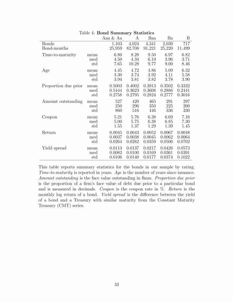
Table 4: Bond Summary StatisticsAaa & Aa A Baa Ba B

Bonds 1,103 4,024 4,341 2,039 717Bond-months 25,959 82,708 91,221 25,220 11,499

Time-to-maturity mean 6.80 8.28 9.50 6.97 6.82med 4.50 4.34 6.19 3.96 3.71std 7.65 10.28 9.77 9.00 8.46

Age mean 4.45 4.72 4.86 5.09 6.32med 3.30 3.74 3.92 4.11 5.58std 3.94 3.81 3.82 3.78 3.90

Proportion due prior mean 0.5003 0.4002 0.3913 0.3502 0.3332med 0.5444 0.3623 0.3608 0.2886 0.2441std 0.2758 0.2795 0.2824 0.2777 0.3016

Amount outstanding mean 527 420 465 291 297med 250 296 350 225 200std 860 516 446 336 330

Coupon mean 5.21 5.76 6.38 6.69 7.16med 5.00 5.75 6.38 6.85 7.30std 1.55 1.37 1.29 1.39 1.45

Return mean 0.0045 0.0043 0.0052 0.0067 0.0048med 0.0037 0.0038 0.0045 0.0062 0.0064std 0.0264 0.0282 0.0359 0.0506 0.0702

Yield spread mean 0.0113 0.0137 0.0217 0.0426 0.0573med 0.0082 0.0100 0.0169 0.0361 0.0391std 0.0106 0.0140 0.0177 0.0374 0.1022

This table reports summary statistics for the bonds in our sample by rating.Time-to-maturity is reported in years. Age is the number of years since issuance.Amount outstanding is the face value outstanding in $mm. Proportion due prioris the proportion of a firm’s face value of debt due prior to a particular bondand is measured in decimals. Coupon is the coupon rate in %. Return is themonthly log return of a bond. Yield spread is the difference between the yieldof a bond and a Treasury with similar maturity from the Constant MaturityTreasury (CMT) series.

33

Table 5: Firm Summary StatisticsAaa & Aa A Baa Ba B

Firms 50 225 468 228 116Firm-months 2,289 10,761 18,200 5,391 2,456Observations 25,959 82,708 91,221 25,220 11,499

Equity market cap mean 204.96 45.51 23.11 10.32 8.14med 173.27 34.32 15.73 10.13 5.98std 121.71 42.89 27.37 7.90 8.46

Equity volatility mean 0.2686 0.2789 0.3255 0.4001 0.4317med 0.2035 0.2459 0.2737 0.3460 0.3647std 0.1614 0.1255 0.1659 0.1849 0.1912

DD leverage mean 0.3315 0.2319 0.2638 0.4417 0.5213med 0.3966 0.1553 0.2092 0.3468 0.4756std 0.2370 0.2043 0.2083 0.3044 0.2522

Pseudo-leverage mean 0.3973 0.3094 0.3616 0.5376 0.6313med 0.4816 0.2408 0.3257 0.4969 0.6327std 0.2583 0.2131 0.2116 0.2829 0.2224

Book-to-market mean 0.39 0.41 0.61 0.91 0.79med 0.31 0.35 0.52 0.73 0.70std 0.22 0.27 0.36 0.62 0.54

Distance-to-default mean 10.24 9.63 8.01 5.87 4.55med 10.80 9.07 7.60 5.09 4.30std 5.44 4.37 3.77 3.00 2.24

Equity Return mean 0.0020 0.0072 0.0059 -0.0018 -0.0090med 0.0053 0.0121 0.0128 0.0080 0.0029std 0.0837 0.0805 0.0994 0.1362 0.1665

This table reports firm characteristics for our sample. Equity market cap is theequity market capitalization in $bn. Equity volatility is the volatility of a firm’sequity using daily log returns over the past year, annualized. DD Leverage is theface value of debt divided by the sum of the face value of debt and the marketvalue of equity. Following Campbell, Hilscher, and Szilagyi (2008), the face valueof debt is defined as Debt in Current Liabilities plus one-half times Long-TermDebt. Pseudo-leverage is defined similarly as DD Leverage, but uses the sum ofDebt in Current Liabilities and Long-Term Debt as the face value of debt. Book-to-market is the book value of equity divided by the market value of equity as inAsness and Frazzini (2011). Distance-to-default is calculated following Campbell,Hilscher, and Szilagyi (2008). Equity Return is the monthly log equity return.

34

Table 6: Co-movement between Corporate Bonds and EquitiesAaa & Aa A Baa Ba B

rE 0.0489 0.0470 0.0886 0.1161 0.1260[9.70] [2.99] [4.73] [7.18] [8.87]

rT 0.6632 0.5779 0.4022 -0.0249 -0.1488[15.62] [8.80] [4.94] [-0.24] [-1.32]

Constant 0.0025 0.0024 0.0034 0.0071 0.0066[4.24] [2.45] [2.19] [4.33] [3.50]

R2 0.2386 0.2128 0.1203 0.1335 0.1695Obs 25,959 82,708 91,221 25,220 11,499

This table reports a regression of rD = β0 + βErE + βT rT . rD, rE, andrT are log returns (in decimals) for corporate bonds, equities, and Trea-suries, respectively. t-statistics are reported in brackets using standarderrors that are clustered by firm and month.

35

Table 7: Co-movement and Maturity StructureAaa & Aa A Baa Ba B

rE × prop due prior 0.0854 0.0468 0.0908 0.1621 0.0348[2.45] [2.95] [2.60] [4.40] [1.03]

rE -0.0044 0.0120 0.0355 0.0786 0.0956[-1.27] [1.99] [4.92] [7.49] [8.04]

rT 0.6683 0.5842 0.4164 -0.0195 -0.1154[16.07] [8.78] [5.12] [-0.18] [-1.07]

rE × T 0.0019 0.0029 0.0023 -0.0034 0.0047[1.98] [1.34] [1.02] [-1.08] [2.64]

rE × T 2 -0.0000 -0.0000 -0.0000 0.0000 -0.0001[-1.32] [-1.49] [-0.60] [0.78] [-3.60]

prop due prior 0.0020 -0.0001 -0.0006 0.0029 0.0000[1.29] [-0.17] [-0.40] [1.27] [0.01]

T -0.0000 0.0000 0.0001 -0.0002 -0.0000[-0.30] [0.18] [0.44] [-1.00] [-0.15]

T 2 0.0000 0.0000 -0.0000 0.0000 0.0000[0.66] [0.06] [-0.68] [1.08] [1.90]

Constant 0.0015 0.0022 0.0031 0.0070 0.0063[7.16] [6.25] [4.85] [8.22] [4.27]

R2 0.2471 0.2192 0.1336 0.1448 0.1776Obs 25,959 82,708 91,221 25,220 11,499

This table reports a regression of rD = β0 + β1rE × prop due prior + βErE +βT rT +β2rE×T +β3rE×T 2 +β4prop due prior+β5T +β6T

2. prop due prioris the proportion of a firm’s face value of debt due prior to a particular bondand is measured in decimals. rD, rE, and rT are log returns (in decimals) forcorporate bonds, equities, and Treasuries, respectively. T is the maturity ofa bond in years. t-statistics are reported in brackets using standard errorsthat are clustered by firm and month.

36

Table 8: Co-movement and Book-to-MarketAaa & Aa A Baa Ba B

rE ×B/M 0.0543 0.0114 0.0252 0.0168 0.0062[5.78] [6.10] [4.22] [3.03] [1.00]

rE 0.0248 0.0238 0.0302 0.0747 0.0958[4.24] [2.91] [3.11] [4.99] [6.88]

rT 0.6731 0.5842 0.4143 -0.0212 -0.1239[16.90] [8.79] [5.14] [-0.20] [-1.02]

rE × T 0.0063 0.0047 0.0060 0.0039 0.0063[3.95] [2.32] [3.64] [1.55] [3.42]

rE × T 2 -0.0001 -0.0001 -0.0000 -0.0000 -0.0001[-2.86] [-2.35] [-2.57] [-1.46] [-2.69]

B/M 0.0008 -0.0003 -0.0003 0.0012 0.0007[1.15] [-1.20] [-0.64] [3.18] [1.25]

T 0.0001 0.0000 0.0000 -0.0000 -0.0000[0.93] [0.10] [0.26] [-0.11] [-0.37]

T 2 0.0000 0.0000 -0.0000 0.0000 0.0000[0.17] [0.10] [-0.56] [0.40] [0.54]

Constant 0.0022 0.0021 0.0033 0.0063 0.0061[14.70] [4.39] [4.82] [7.15] [3.35]

R2 0.2518 0.2208 0.1385 0.1449 0.1830Obs 25,959 81,720 89,896 24,456 8,955

This table reports a regression of rD = β0 + β1rE × B/M + βErE +βT rT +β2rE×T +β3rE×T 2 +β4B/M +β5T +β6T

2. B/M is the book-to-market ratio of a firm, winsorized at 1% of each tail and normalizedby the cross-sectional mean and standard deviation each month. rD,rE, and rT are log returns (in decimals) for corporate bonds, equities,and Treasuries, respectively. T is the maturity of a bond in years.t-statistics are reported in brackets using standard errors that are clus-tered by firm and month.

37

Table 9: Co-movement and Distance-to-DefaultAaa & Aa A Baa Ba B

rE ×DD -0.0164 -0.0155 -0.0307 -0.0502 -0.0292[-5.26] [-3.08] [-3.44] [-3.71] [-1.21]

rE 0.0133 0.0178 0.0326 0.0444 0.0594[1.38] [2.63] [3.86] [2.33] [1.86]

rT 0.6683 0.5824 0.4152 -0.0190 -0.1193[16.04] [8.79] [5.15] [-0.18] [-1.09]

rE × T 0.0063 0.0049 0.0055 0.0038 0.0064[3.46] [2.50] [3.28] [1.52] [4.05]

rE × T 2 -0.0001 -0.0001 -0.0000 -0.0000 -0.0001[-2.69] [-2.41] [-2.32] [-1.34] [-4.10]

DD -0.0006 0.0000 -0.0001 -0.0023 0.0014[-1.63] [0.21] [-0.13] [-3.20] [0.87]

T 0.0001 0.0000 0.0000 -0.0000 -0.0000[1.10] [0.13] [0.32] [-0.21] [-0.34]

T 2 0.0000 0.0000 -0.0000 0.0000 0.0000[0.01] [0.11] [-0.61] [0.47] [1.11]

Constant 0.0023 0.0022 0.0031 0.0054 0.0083[4.01] [5.03] [4.29] [5.96] [2.72]

R2 0.2477 0.2200 0.1356 0.1424 0.1784Obs 25,959 82,457 90,361 25,139 11,300

This table reports a regression of rD = β0+β1rE×DD+βErE+βT rT +β2rE×T+β3rE×T 2+β4DD+β5T+β6T

2. DD is the distance-to-defaultof a firm, winsorized at 1% of each tail and normalized by the cross-sectional mean and standard deviation each month. rD, rE, and rT arelog returns (in decimals) for corporate bonds, equities, and Treasuries,respectively. T is the maturity of a bond in years. t-statistics arereported in brackets using standard errors that are clustered by firmand month.

38

Fig

ure

1:H

edge

Rat

ios

for

the

Mer

ton,

Exte

nded

Mer

ton,

and

Ges

kem

odel

s.F

orpan

els

(b)

and

(c),

the

cyan

surf

aces

repre

sent

the

case

wher

ea

bon

dis

late

init

sfirm

’sm

aturi

tyst

ruct

ure

and

the

red

surf

aces

wit

hp

oint

mar

kers

repre

sent

the

case

wher

ea

bon

dis

earl

yin

its

firm

’sm

aturi

tyst

ruct

ure

.

39

Appendix

A Merton Model with Seniority

As discussed by Black and Cox (1976) and Lando (2004) among others, for a firm with a

zero-coupon junior bond with a face value of KJ and a zero-coupon senior bond with a face

value of KS (both maturing at T ), the values of the junior and senior bonds are

BJ = V N(d1,S)−KSe−rTN(d2,s)− V N(d1) +Ke−rTN(d2), (13)

BS = V − V N(d1,S) +KSe−rTN(d2,S),

where d1,S =ln(

VKS

)+(r + 1

2σ2v

)T

σv√T

, d2,S = d1,S − σv√T ,

and d1 =ln(

VKS+KJ

)+(r + 1

2σ2v

)T

σv√T

, d2 = d1 − σv√T .

It can be shown that

∂ lnBJ

∂ lnV− ∂ lnBS

∂ lnV=

V

BS ×BJ

[BS (N(d1,S)−N(d1))−BJ (1−N(d1,S))] > 0. (14)

B Merton Model with Maturity Structure

In our extension of the Merton model, the firm has three zero coupon bond issues with face

values K1, K2, and K3, and maturities T1 < T2 < T3. All of the bonds share the same

seniority. For example, suppose that the firm defaults prior to T1. The proportion of the

total recovered value of the firm that is paid to bond 1 is K1

K1+K2+K3. In addition, we also

allow for a proportion L of the residual firm value to be lost in bankruptcy. That is, if the

value of the firm at default is Vdefault, the proportion payable to bondholders is (1−L)Vdefault.

40

B.1 Equity Value

E = EQ0

[e−rT31V1>K11V2>K21V3>K3 (V3 −K3)

]The firm value process is lognormal

V1 = V0 exp

[(r − 1

2σ2v

)T1 + σv

√T1w1

], (15)

where w1 ∼ N(0, 1).

Similarly,

V2 = (V1 −K1) exp

[(r − 1

2σ2v

)(T2 − T1) + σv

√T2 − T1w2

]if V1 > K1

and

V3 = (V2 −K2) exp

[(r − 1

2σ2v

)(T3 − T2) + σv

√T3 − T2w3

]if V2 > K2

After some algebra, it can be shown that

E =e−rT2

2π

∫ ∞−d2

∫ ∞−d̃2

exp

(−1

2z22 −

1

2z21

)(V2 −K2)N

(˜̃d1

)dz2dz1 (16)

−K3−e−rT3

2π

∫ ∞−d2

∫ ∞−d̃2

exp

(−1

2z22 −

1

2z21

)N(

˜̃d2

)dz2dz1,

where ˜̃d2 =ln(V2−K2

K3

)+(r − 1

2σ2v

)(T3 − T2)

σv√T3 − T2

, ˜̃d1 = ˜̃d2 + σv√T3 − T2

and d̃2 =ln(V1−K1

K2

)+(r − 1

2σ2v

)(T2 − T1)

σv√T2 − T1

.

41

B.2 Bond Value

Our focus is on the intermediate bond with maturity T2 and face value K2. The price of this

bond can be written as the sum of three expectations, which correspond to (1) solvency at

T2, (2) default at T1, and (3) default at T2. The value of each of these pieces corresponds to

1. EQ0

[e−rT21V1>K11V2>K2K2

];

2. EQ0

[e−rT21V1<K1(1− L)V1

K2

K1+K2+K3

]; and

3. EQ0

[e−rT21V1>K11V2<K2(1− L)V2

K2

K2+K3

].

After some algebra, it can be shown that the three pieces are

1. K2e−rT2√

2π

∫ ∞−d2

exp(−1

2z21)N(d̃2

)dz1;

2. V0(1− L) K2

K1+K2+K3N(−d1); and

3. K2(1−L)e−rT1

(K2+K3)√2π

∫ ∞−d2

exp(−1

2z21)

(V1 −K1)N(−d̃1

)dz1.

B.3 Hedge Ratios

In principle, numerical partial derivatives can be calculated once we have bond prices. How-

ever, in our implementation of the extended Merton model, we find that numerical partial

derivatives calculated for prices that are determined though numerical integration can be-

come quite imprecise. Thus, we apply Leibniz’s rule to first calculate partial derivatives as

functions of integrals (much like the bond prices themselves) before numerically integrating.

In particular, the three pieces of the partial derivative of the bond price (from B.2) with

respect to firm value (∂B/∂V ) are

1. K2e−rT2

∫ ∞−d2

1√2πexp

(−1

2z21)n(d̃2

)V1V0

1(V1−K1)σv

√T2−T1

dz1;

2. (1−L)K2N(−d1)K1+K2+K3

− (1−L)K2n(−d1)(K1+K2+K3)σv

√T1

; and

3. (1−L)K2e−rT1

K2+K3

[∫ ∞−d2

1√2πexp

(−1

2z21)V1V0N(−d̃1

)dz1 −

∫ ∞−d2

1√2πexp

(−1

2z21) (V1−K1)n(−d̃1)V1σv√T2−T1(V1−K1)V0

dz1

].

42

The hedge ratio can then be calculated by taking ∂B∂V

VB

and dividing by the numerically

calculated ∂E∂V

VE

.

C Extending the Geske Model

The two models in our paper, the extended Merton model and the Geske model, make very

different assumptions about how maturing bonds are paid off. In the extended Merton model,

a maturing bond is paid from firm assets, whereas in the Geske model, equityholders pay the

full face value of the maturing bond. Here, we consider allowing the maturing bond to be

paid partially from firm assets and partially by equityholders. Define α to be the proportion

of the maturing bond face value that can be paid from firm assets. If αKt ≤ Vt, αKt is paid

from firm assets and equityholders decide whether to pay (1− α)Kt to continue the firm.

The extended Merton and Geske models are the two special cases that correspond to

α = 1 and α = 0, respectively. In the extended Merton model, equityholders always continue

the firm if Vt > Kt, whereas in the Geske model, equityholders sometimes choose to default

even if Vt > Kt because the pay-in to continue the firm is too high relative to the value of

their potential future payoff. Whether decreasing the equity pay-in significantly increases

the likelihood of equityholders continuing the firm is unclear as the decreased pay-in comes

at the cost of decreasing firm value. To illustrate the point, suppose that a firm has a zero-

coupon bond maturing at time T2 with a face value of 20 and another zero-coupon bond

maturing at time T3 = T2 + 3 with a face value of 30. Suppose that the firm value is 45 at T2

and it only has these two bond issues outstanding. Naturally, at α = 1, equityholders always

continue the firm. If α = 0, equityholders need to decide whether to pay 20 in exchange

for a call option maturing in three years with a strike of 30 and a current underlying asset

value of 45. In this case, the value of the call option is 17.25 and equityholders choose to

let the firm default. Consider instead α = 0.5. In this case, equityholders only need to pay

(1 − α) × 20 = 10 to continue the firm. However, the other 10 is paid out of firm value, so

43

equityholders are deciding whether to buy a call option with a strike of 30 and an underlying

asset value of 35. Despite the decreased pay-in, equityholders still choose to let the firm

default because the value of the call option is only worth 8.52 due to the option being less

in-the-money than before. In Figure A.1, we plot the value of the call option and the cost to

equityholders to continue the firm. By definition, between the two extreme cases of α = 0

and α = 1, there is an α ∈ [0, 1] where equityholders are indifferent. In this example, this α

is slightly less than 0.8.

In Figure A.2, we plot the difference between the hedge ratios of the intermediate maturity

bond when most of the firm’s debt is due before the bond and when most of the firm’s debt is

due after the bond for different levels of α, using the same parameters as in Section 2. For low

values of α, the difference in hedge ratios between the two scenarios is close to 0. At α = 0.8,

we begin to see some evidence of de facto seniority, as the hedge ratio of the intermediate

maturity bond when most of the firm’s debt is due before it becomes higher. What drives

the relatively high α needed to generate de facto seniority is that there is typically a wide set

of asset values where Vi is not much larger than Ki and the continuation value of equity is

low. Any non-trivial required pay-in by equityholders would result in equityholders choosing

default, whereas a zero pay-in (α = 1) would lead to continuation.

D Robustness Checks

D.1 Firm-level Maturity

Recent theoretical literature has examined the equilibrium choice of debt maturity by firms.

Brunnermeier and Oehmke (2013) solve a model where the equilibrium is a maturity rate

race and the outcome is an inefficiently large amount of short-maturity bonds. Chen, Xu,

and Yang (2012) use a model to show that firms with higher systematic volatility choose

longer-maturity bonds and find empirical support for this prediction. We note that these

studies are about aggregate firm-level maturity choice, while our focus is on how the relative

44

maturity of a bond compared to the rest of the bonds issued by the same issuer. Nevertheless,

we repeat our analysis after controlling for the average firm-level maturity in Table A.1. We

find that our de facto seniority results from Table 7 are largely unchanged. Specifically,

there are few differences in the economic and statistical significance for the coefficient on

rE × prop due prior.

D.2 Liquidity Measures

Though the structural models of default considered here do not allow for a natural role for

liquidity to affect hedge ratios, we acknowledge that many papers have shown that bond

illiquidity affects corporate bond pricing. Thus, we control for the Amihud (2002) illiquidity

measure in Table A.2. We find that our baseline results are unchanged. Interestingly,

we also find that hedge ratios are larger for more illiquid bonds. This can potentially be

explained by the He and Xiong (2012) and He and Milbradt (2013) findings that illiquidity

can introduce additional credit risk. This additional credit risk leads to additional exposure

to the underlying firm value, increasing the hedge ratio.

45

Table A.1: Firm-level MaturityAaa & Aa A Baa Ba B

rE × prop due prior 0.0871 0.0540 0.1148 0.1791 0.0599[2.02] [2.14] [2.99] [3.63] [2.74]

rE × avg firm mat 0.0002 0.0006 0.0019 0.0024 0.0039[0.15] [0.64] [1.83] [0.81] [1.96]

rE -0.0066 0.0055 0.0141 0.0565 0.0603[-0.49] [0.61] [1.08] [2.14] [2.41]

rT 0.6681 0.5842 0.4170 -0.0175 -0.1136[16.12] [8.78] [5.13] [-0.17] [-1.05]

rE × T 0.0018 0.0025 0.0011 -0.0045 0.0034[2.11] [1.05] [0.46] [-1.15] [3.58]

rE × T 2 -0.0000 -0.0000 -0.0000 0.0000 -0.0001[-1.31] [-1.26] [-0.16] [0.89] [-4.31]

R2 0.2472 0.2193 0.1339 0.1456 0.1791Obs 25,959 82,708 91,221 25,220 11,499

This table reports regressions of corporate bond returns on equity returns and other controls.avg firm mat is the average remaining time-to-maturity for a bond issuer, weighted byamount outstanding. Other variables are as defined in Table 7. Additional unreportedcontrols are prop due prior, avg firm mat, T , T 2, and a constant term. t-statistics arereported in brackets using standard errors that are clustered by firm and month.

46

Table A.2: LiquidityAaa & Aa A Baa Ba B

rE × prop due prior 0.0630 0.0548 0.0999 0.1438 0.0226[2.14] [3.61] [3.03] [4.32] [0.57]

rE × Amihud 0.0175 0.0092 0.0242 0.0308 0.0120[2.84] [1.73] [3.04] [2.36] [1.22]

rE -0.0084 0.0087 0.0266 0.0632 0.0878[-2.11] [1.53] [4.09] [6.70] [7.48]

rT 0.6637 0.5797 0.4126 -0.0323 -0.1113[15.11] [8.33] [5.20] [-0.31] [-1.06]

rE × T 0.0027 0.0022 0.0019 -0.0024 0.0058[2.68] [1.03] [0.81] [-0.80] [2.97]

rE × T 2 -0.0000 -0.0000 -0.0000 0.0000 -0.0001[-2.01] [-0.93] [-0.42] [0.36] [-3.94]

R2 0.2548 0.2261 0.1425 0.1551 0.1855Obs 23,667 74,068 82,831 23,502 10,758

This table reports regressions of corporate bond returns on equity returns and other controls.Amihud is the Amihud (2002) measure. Other variables are as defined in Table 7. Additionalunreported controls are prop due prior, Amihud, T , T 2, and a constant term. t-statistics arereported in brackets using standard errors that are clustered by firm and month.

47

0 0.1 0.2 0.3 0.4 0.5 0.6 0.7 0.8 0.9 10

2

4

6

8

10

12

14

16

18

20

α

Val

ue

Required payment by equityholdersValue of option

Figure A.1: Dashed line is the amount that equityholders need to pay-in to continue thefirm for different levels of α. Dashed curve is the value of the call option that equityholderswould hold if they choose to continue the firm.

48

Fig

ure

A.2

:H

edge

Rat

ios

for

the

the

exte

nded

Ges

kem

odel

.T

he

pan

els

plo

tdiff

eren

ces

bet

wee

nth

ehed

gera

tios

ofth

ein

term

edia

tem

aturi

tyb

ond

when

mos

tof

the

firm

’sdeb

tis

due

bef

ore

the

bon

dan

dw

hen

mos

tof

the

firm

’sdeb

tis

due

afte

rth

eb

ond.α

repre

sents

the

pro

por

tion

ofth

ein

term

edia

tem

aturi

tyb

ond’s

face

valu

eth

atis

pai

dfr

omfirm

asse

ts.

49

References

Adelino, M. (2009). Do Investors Rely Only on Ratings? The Case of Mortgage-BackedSecurities. Working Paper, Duke.

Amihud, Y. (2002). Illiquidity and stock returns: cross-section and time-series effects.Journal of Financial Markets 5, 31–56.

Asness, C. and A. Frazzini (2011). The Devil in HML’s Details. Working Paper, AQRCapital Management.

Baele, L., G. Bekaert, and K. Inghelbrech (2010). The Determinants of Stock and BondReturn Comovements. Review of Financial Studies 23, 2374–2428.

Baker, M. and J. Wurgler (2012). Comovement and Predictability Relationships BetweenBonds and the Cross-section of Stocks. Review of Asset Pricing Studies 2, 57–87.

Bao, J. and J. Pan (2013). Bond Illiquidity and Excess Volatility. Review of FinancialStudies 26, 3068–3103.

Bao, J., J. Pan, and J. Wang (2011). The Illiquidity of Corporate Bonds. Journal ofFinance 66, 911–946.

Bharath, S. T. and T. Shumway (2008). Forecasting Default with the Merton Distance toDefault Model. Review of Financial Studies 21, 1339–1369.

Black, F. and J. C. Cox (1976). Valuing Corporate Securities: Some Effects of BondIndenture Provisions. Journal of Finance 31, 351–367.

Brunnermeier, M. K. and M. Oehmke (2013). The Maturity Rat Race. Journal of Fi-nance 68, 483–521.

Campbell, J. Y., J. Hilscher, and J. Szilagyi (2008). In Search of Distress Risk. Journal ofFinance 63, 2899–2939.

Campbell, J. Y., C. Pflueger, and L. M. Viciera (2013). Monetary Policy Drivers of Bondand Equity Risks. Working Paper, Harvard and UBC.

Chen, H., Y. Xu, and J. Yang (2012). Systematic Risk, Debt Maturity, and the TermStructure of Credit Spreads. Working Paper, MIT and Bank of Canada.

Chen, L., P. Collin-Dufresne, and R. S. Golstein (2009). On the Relation Between theCredit Spread Puzzle and the Equity Premium Puzzle. Review of Financial Studies 22,3367–3409.

Chen, L., D. Lesmond, and J. Wei (2007). Corporate Yield Spreads and Bond Liquidity.Journal of Finance 62, 119–149.

Collin-Dufresne, P. and R. S. Goldstein (2001). Do Credit Spreads Reflect StationaryLeverage Ratios? Journal of Finance 56, 1929–1957.

Collin-Dufresne, P., R. S. Goldstein, and J. Helwege (2010). Is Credit Event Risk Priced?Modeling Contagion via the Updating of Beliefs. Working Paper, Columbia, Minnesota,and South Carolina.

Collin-Dufresne, P., R. S. Goldstein, and S. Martin (2001). The Determinants of CreditSpread Changes. Journal of Finance 56, 2177–2207.

50

Cox, J. C., S. A. Ross, and M. Rubinstein (1979). Option Pricing: A Simplified Approach.Journal of Financial Economics 7, 229–263.

Crosbie, P. and J. Bohn (2003). Modeling Default Risk. Working Paper, Moody’s KMV.

Daniel, K. and S. Titman (1997). Evidence on the Characteristics of Cross SectionalVariation in Stock Returns. Journal of Finance 52, 1–33.

Dick-Nielsen, J., P. Feldhutter, and D. Lando (2012). Corporate bond liquidity before andafter the onset of the subprime crisis. Journal of Financial Economics 103, 471–492.

Duffie, D. and D. Lando (2001). Term Structures of Credit Spreads with IncompleteAccounting Information. Econometrica 69, 633–664.

Edwards, A. K., L. E. Harris, and M. S. Piwowar (2007). Corporate Bond Market Trans-action Costs and Transparency. Journal of Finance 62, 1421–1451.

Eom, Y. H., J. Helwege, and J. Z. Huang (2004). Structural Models of Corporate BondPricing: An Empirical Analysis. Review of Financial Studies 17, 499–544.

Fama, E. F. and K. R. French (1993). Common risk factors in the returns on stocks andbonds. Journal of Financial Economics 33, 3–56.

Fama, E. F. and K. R. French (1995). Size and Book-to-Market Factors in Earnings andReturns. Journal of Finance 50, 131–155.

Fama, E. F. and K. R. French (1996). Multifactor Explanations of Asset Pricing Anomalies.Journal of Finance 51, 55–84.

Feldhutter, P. (2012). The same bond at different prices: identifying search frictions andselling pressures. Review of Financial Studies 25, 1155–1206.

Geske, R. (1977). The Valuation of Corporate Liabilities as Compound Options. Journalof Financial and Quantitative Analysis 12, 541–552.

Haugen, R. A. (1995). The new finance – The case against efficient markets. Prentice-Hall.

He, Z. and K. Milbradt (2013). Endogenous Liquidity and Defaultable Bonds. Economet-rica, forthcoming .

He, Z. and W. Xiong (2012). Rollover Risk and Credit Risk. Journal of Finance 67, 391–429.

Hillegeist, S. A., E. Keating, D. Cram, and K. Lundstedt (2004). Assessing the Probabilityof Bankruptcy. Review of Accounting Studies 9, 5–34.

Hotchkiss, E. H. and T. Ronen (2002). The Informational Efficiency of the CorporateBond Market: An Intraday Analysis. Review of Financial Studies 15, 1325–1354.

Hou, K. and M. A. van Dijk (2012). Profitability shocks and the size effect in the cross-section of expected stock returns. Working Paper, Ohio State and Erasmus.

Huang, J. Z. (1997). Default Risk, Renegotiation, and the Valuation of Corporate Claims.Ph. D. thesis, NYU.

Huang, J. Z. and M. Huang (2003). How Much of the Corporate-Treasury Yield Spread isDue to Credit Risk. Working Paper, Penn State and Stanford.

51

Huang, J. Z. and Z. Shi (2013). A Revisit to the Equity-Credit Market IntegrationAnomaly. Working Paper, Penn State.

Kwan, S. H. (1996). Firm Specific Information and the Correlation Between IndividualStocks and Bonds. Journal of Financial Economics 40, 63–80.

Lakonishok, J., A. Shleifer, and R. W. Vishny (1994). Contrarian Investment, Extrapola-tion, and Risk. Journal of Finance 49, 1541–1578.

Lando, D. (2004). Credit Risk Modeling. Princeton University Press.

Leland, H. E. (1994). Corporate Debt Value, Bond Covenants, and Optimal Capital Struc-ture. Journal of Finance 49, 157–196.

Leland, H. E. and K. Toft (1996). Optimal Capital Structure, Endogenous Bankruptcy,and the Term Structure of Credit Spreads. Journal of Finance 51, 987–1019.

Longstaff, F. A. and E. S. Schwartz (1995). A Simple Approach to Valuing Risky Fixedand Floating Rate Debt. Journal of Finance 50, 789–819.

MacKinlay, A. C. (1995). Multifactor models do not explain deviations from the CAPM.Journal of Financial Economics 38, 3–28.

Masulis, R. W. and A. N. Korwar (1986). Seasoned Equity Offerings: An Empirical In-vestigation. Journal of Financial Economics 15, 91–118.

Maxwell, W. F. and R. Rao (2003). Do Spin-offs Expropriate Wealth from Bondholders?Journal of Finance 58, 2087–2108.

Maxwell, W. F. and C. Stephens (2003). The Wealth Effects of Repurchases on Bondhold-ers. Journal of Finance 58, 895–919.

Merton, R. C. (1974). On the Pricing of Corporate Debt: The Risk Structure of InterestRates. Journal of Finance 29, 449–470.

Powers, E. A. and S. Tsyplakov (2008). What is the Cost of Financial Flexibility? Theoryand Evidence from Make-whole Call Provisions. Financial Management 37, 485–512.

Rauh, J. D. and A. Sufi (2010). Capital Structure and Debt Structure. Review of FinancialStudies 23, 4242–4280.

Schaefer, S. M. and I. A. Strebulaev (2008). Structural Models of Credit Risk are Useful:Evidence from Hedge Ratios on Corporate Bonds. Journal of Financial Economics 90,1–19.

Shimko, D. C., N. Tejima, and D. R. van Deventer (1993). The Pricing of Risky Debtwhen Interest Rates are Stochastic. Journal of Fixed Income 3, 58–65.

Vassalou, M. and Y. Xing (2004). Default Risk in Equity Returns. Journal of Finance 59,831–868.

52