credit chain and sectoral comovement
TRANSCRIPT
ASIAN DEVELOPMENT BANK
ADB ECONOMICSWORKING PAPER SERIES
NO. 640
October 2021
CREDIT CHAIN AND SECTORAL COMOVEMENTA MULTI-REGION INVESTIGATION
Hsiao-Hui Lee, S. Alex Yang, Yuxuan Zhang, and Kijin Kim
ASIAN DEVELOPMENT BANK
ADB Economics Working Paper Series
Credit Chain and Sectoral Comovement: A Multi-Region Investigation
Hsiao-Hui Lee, S. Alex Yang, Yuxuan Zhang, and Kijin Kim
No. 640 | October 2021
Hsiao-Hui Lee ([email protected]) is a professor at the College of Commerce, National Chengchi University. S. Alex Yang ([email protected]) is an associate professor of Management Science and Operations at the London Business School. Yuxuan Zhang ([email protected]) is an assistant professor at the University of International Business and Economics. Kijin Kim ([email protected]) is an economist at the Economic Research and Regional Cooperation Department, Asian Development Bank.

Creative Commons Attribution 3.0 IGO license (CC BY 3.0 IGO)
© 2021 Asian Development Bank6 ADB Avenue, Mandaluyong City, 1550 Metro Manila, PhilippinesTel +63 2 8632 4444; Fax +63 2 8636 2444www.adb.org
Some rights reserved. Published in 2021.
ISSN 2313-6537 (print), 2313-6545 (electronic)Publication Stock No. WPS210391-2DOI: http://dx.doi.org/10.22617/WPS210391-2
The views expressed in this publication are those of the authors and do not necessarily reflect the views and policies of the Asian Development Bank (ADB) or its Board of Governors or the governments they represent.
ADB does not guarantee the accuracy of the data included in this publication and accepts no responsibility for any consequence of their use. The mention of specific companies or products of manufacturers does not imply that they are endorsed or recommended by ADB in preference to others of a similar nature that are not mentioned.
By making any designation of or reference to a particular territory or geographic area, or by using the term “country” in this document, ADB does not intend to make any judgments as to the legal or other status of any territory or area.
This work is available under the Creative Commons Attribution 3.0 IGO license (CC BY 3.0 IGO) https://creativecommons.org/licenses/by/3.0/igo/. By using the content of this publication, you agree to be bound by the terms of this license. For attribution, translations, adaptations, and permissions, please read the provisions and terms of use at https://www.adb.org/terms-use#openaccess.
This CC license does not apply to non-ADB copyright materials in this publication. If the material is attributed to another source, please contact the copyright owner or publisher of that source for permission to reproduce it. ADB cannot be held liable for any claims that arise as a result of your use of the material.
Please contact [email protected] if you have questions or comments with respect to content, or if you wish to obtain copyright permission for your intended use that does not fall within these terms, or for permission to use the ADB logo.
Corrigenda to ADB publications may be found at http://www.adb.org/publications/corrigenda.
Notes: In this publication, “$” refers to United States dollars. ADB recognizes “Vietnam” as Viet Nam.
The ADB Economics Working Paper Series presents data, information, and/or findings from ongoing research and studies to encourage exchange of ideas and to elicit comment and feedback about development issues in Asia and the Pacific. Since papers in this series are intended for quick and easy dissemination, the content may or may not be fully edited and may later be modified for final publication.

CONTENTS
TABLES AND FIGURES iv ABSTRACT v I. INTRODUCTION 1 II. THE MODEL 3 III. DATA AND VARIABLE CONSTRUCTIONS 6 A. The Use of Trade Credit (Matrix P) 7 B. Input-Output Linkages (B and D) 8 C. Sectoral Correlations (ρ) 10 IV. EMPIRICAL RESULTS 13 A. Base Results 13 B. Robustness 14 C. Time Variation 14 D. Trade Credit Financing versus Bank Credit Financing 21 V. POLICY IMPLICATIONS AND CONCLUSIONS 24 REFERENCES 25
TABLES AND FIGURES
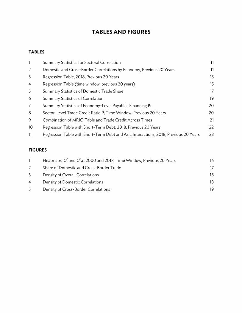
TABLES 1 Summary Statistics for Sectoral Correlation 11 2 Domestic and Cross-Border Correlations by Economy, Previous 20 Years 11 3 Regression Table, 2018, Previous 20 Years 13 4 Regression Table (time window: previous 20 years) 15 5 Summary Statistics of Domestic Trade Share 17 6 Summary Statistics of Correlation 19 7 Summary Statistics of Economy-Level Payables Financing Pn 20 8 Sector-Level Trade Credit Ratio Pj, Time Window: Previous 20 Years 20 9 Combination of MRIO Table and Trade Credit Across Times 21 10 Regression Table with Short-Term Debt, 2018, Previous 20 Years 22 11 Regression Table with Short-Term Debt and Asia Interactions, 2018, Previous 20 Years 23 FIGURES 1 Heatmaps: CD and CF at 2000 and 2018, Time Window, Previous 20 Years 16 2 Share of Domestic and Cross-Border Trade 17 3 Density of Overall Correlations 18 4 Density of Domestic Correlations 18 5 Density of Cross-Border Correlations 19
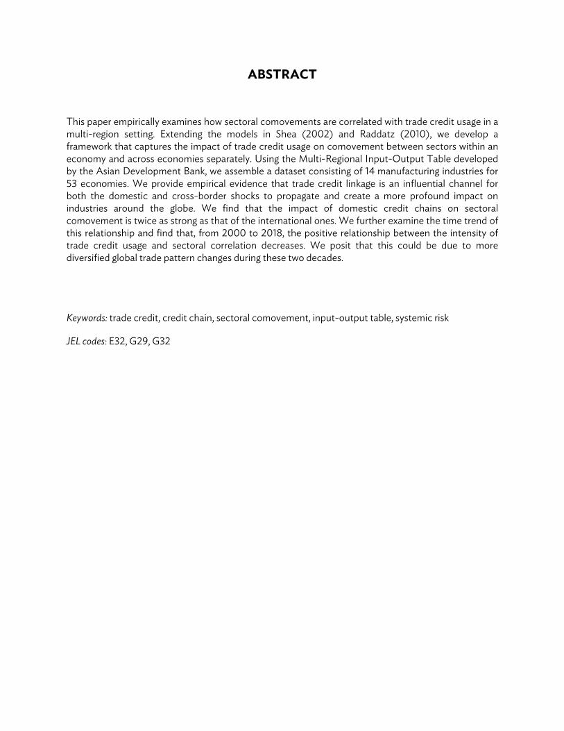
ABSTRACT
This paper empirically examines how sectoral comovements are correlated with trade credit usage in a multi-region setting. Extending the models in Shea (2002) and Raddatz (2010), we develop a framework that captures the impact of trade credit usage on comovement between sectors within an economy and across economies separately. Using the Multi-Regional Input-Output Table developed by the Asian Development Bank, we assemble a dataset consisting of 14 manufacturing industries for 53 economies. We provide empirical evidence that trade credit linkage is an influential channel for both the domestic and cross-border shocks to propagate and create a more profound impact on industries around the globe. We find that the impact of domestic credit chains on sectoral comovement is twice as strong as that of the international ones. We further examine the time trend of this relationship and find that, from 2000 to 2018, the positive relationship between the intensity of trade credit usage and sectoral correlation decreases. We posit that this could be due to more diversified global trade pattern changes during these two decades.
Keywords: trade credit, credit chain, sectoral comovement, input-output table, systemic risk
JEL codes: E32, G29, G32
Credit Chain and Sectoral Comovement 1
I. INTRODUCTION
As the volume of global trade nearly quadrupled over the last 2 decades, the global supply chain became increasingly interconnected. This interconnection has allowed companies to lower costs, but it also results in comovement across different sectors and regions. Consequently, a shock originating in one sector or geographic region can cascade into different sectors across the globe.
During the 2011 monsoon, for example, flood water inundated industrial estates in Thailand, hosting considerable global production capacity in a few sectors, causing hundreds of deaths and tremendous economic damage amid disruptions in manufacturing. As Thailand produced about a quarter of total hard drives in the world at that time, the floods caused a global hard drive shortage, pushing up prices and undermining profitability of downstream sectors. Such shocks can also propagate far beyond Thailand: Japanese companies such as Canon, Honda, and Toyota all produce a large share of products and/or components in Thailand, and the flooding hit these companies’ profits and worker incomes in Japan.
An extreme weather event is only one type of shock demonstrating the interconnectedness of global supply chains. The global financial crisis in 2008 and the COVID-19 pandemic have likewise highlighted that sectors and regions are closely linked by the flow of physical goods.
Different sectors and regions also experience comovements due to financial flows between them. One of the most important financial linkages between companies within supply chains is trade credit. As credit extended by sellers to buyers in supply chains, trade credit is one of the most important sources of external financing globally (Rajan and Zingales 1995). It amounted to $5.4 trillion in 2019 in the United States (US), for example, with growth outpacing that of GDP (Federal Reserve Board 2019). As such, it is a financial instrument with macroeconomic significance.
Trade credit also creates credit chains across firms in different sectors of the economy (Kiyotaki and Moore 1998). That is, different sectors in the economy are not only linked through business transactions (sellers and buyers of products and services), but also financially by providing and receiving trade credit from each other. An important implication of such credit chains is that trade credit could serve as an additional channel that links different sectors. Naturally, this would suggest that the intensity of trade credit usage positively influences sectoral correlation. Put differently, if sector A (buyer) receives a lot of trade credit from sector B (supplier), then a shock in sector A could translate into a larger shock in sector B relative to those sector pairs with less trade credit in between.
The above hypothesis was first confirmed empirically by Raddatz (2010) by combining the standard input-output matrix from the US Bureau of Labor Statistics and firm financial data from Worldscope and Compustat. However, data limitations left a few questions unanswered in the paper. First, without a multi-region input and output matrix, Raddatz (2010) exclusively studies transactions within each economy and it is thus unclear whether such credit chains act differently for domestic and international trade. Second, Raddatz (2010) focuses on a single time period in the early 2000s, yet the development of the global supply chain in the last two decades begs the question whether the dynamics between credit chain and sectoral comovement have changed over time. Finally, as an increasingly important powerhouse of the global economy, do Asian economies exhibit any special patterns?
2 ADB Economics Working Paper Series No. 640
To answer the above questions, this paper first extends the model in Shea (2002) and Raddatz (2010) to decompose the impact of trade credit usage on sectoral comovement by domestic and cross-border trade. Specifically, our model allows that the shock propagation via domestic credit chains has a different rate from that via cross-border chains. This allows us to empirically examine whether within- and cross-economy credit chains have different impact on sectoral comovement.
We then construct a new dataset to identify these two effects. Specifically, we triangulate the financial data from Compustat and Worldscope, the input-output table from the Multi-Region Input-Output (MRIO) Database developed by the Asian Development Bank (ADB), the growth rate of real value added using the Industrial Statistics database (INDSTAT) developed by the United Nations Industrial Development Organization (UNIDO), and the consumer price index (CPI) from the World Bank. With these, we construct a data set that consists of 14 industries from 53 economies.
Our empirical results suggest that the use of trade credit indeed positively correlates with sectoral comovement. The intensity of this correlation via the domestic credit chain is twice as strong as that via the cross-border credit chain, and the results are robust to training and the change of time windows in computing sectoral correlations.
Further, we examine how the correlation between trade credit usage and sectoral comovement evolves over time by using different MRIO data at 2000, 2007, 2013, and 2018. We find that both the positive relation between trade-credit usage intensity and correlations decreases. We posit that this could be due to more dissected supply chain structures that enable industries to diversify production as well as trade credit linkage intensity from domestic-based to foreign-based. By ruling out several plausible explanations, we provide robust empirical support for our hypothesis.
The paper contributes to two strands of research: trade credit and sectoral comovement, the former providing a rich and long literature, theoretical and empirical. The literature focuses on explaining the existence of trade credit, that is, why buyers borrow money from sellers in the presence of specialized financial institutions. Nadiri (1969) highlighted that trade credit is used as an effective marketing tool. Subsequent research have identified various reasons why trade credit is adopted, such as suppliers having easier access to financing (Schwartz 1974), price discrimination (Brennan, Miksimovic, and Zechner 1988), quality assurance (Long, Malitz, and Ravid 1993; Babich and Tang 2012), alleviating moral hazard (Burkart and Ellingsen 2004), facilitating relationship specific investment (Cuñat 2007), demand risk-sharing (Kouvelis and Zhao 2012; Yang and Birge 2018), and softening competition (Peura, Yang, and Lai 2017).
Relative to the theoretical literature, the empirical literature of trade credit is relatively new, largely due to data limitations. Earlier research in this field focuses on validating theories of trade credit and identifying determinants of trade credit, such as Petersen and Rajan (1997), Ng, Smith, and Smith (1999), and Giannetti, Burkart, and Ellingsen (2011). In a developing economy setting, McMillan and Woodruff (1999) document that trade credit is closely related to relationship building. Fisman and Love (2003) find that trade credit access could facilitate industry growth. Boissay and Gropp (2013) and Jacobson and Von Schedvin (2015) quantify how trade credit default cascades along the supply chain. Lee, Zhou, and Wang (2018) and Chod, Lyandres, and Yang (2019) examine the interaction between trade credit usage and the horizontal relationship between firms. Most recently, several studies focus on identifying the causal relationship between trade credit and operational and financial performance. Barrot (2016) shows that limiting trade credit provision improves the financial strength of upstream firms; Breza and Liberman (2017) and Chen, Jain, and Yang (2020), on the other hand, find that restricting trade credit provision reduces transaction volume between different firms and undermines downstream firms’ investment and revenues.
Credit Chain and Sectoral Comovement 3
Meanwhile, sectoral comovement is an important topic in macroeconomics. Macroeconomic models in general are concerned with business cycles, both correlated movements in economy-wide output over time and comovement between sectors (Lucas 1995). Long Jr and Plosser (1983) develop a multi-sector economy to capture shocks moving along input-output linkages. The model is extended by Shea (2002). Lilien (1982) points out that labor movement could be another source of linkage between sectoral comovement. Cooper and Haltiwanger (1990) develop a dynamic model to capture the sectoral comovement with inventory and offer empirical evidence to support their theory.
Combining the above two streams of work, the study of Kiyotaki and Moore (1998) is the first to formalize the idea of the credit chain, that is, different sectors are linked financially; this model was extended by Cardoso-Lecourtois (2004) and Boissay (2006). These studies highlight that, through trade credit, sectoral shocks can move both from upstream to downstream, and the other way around. Finally, Raddatz (2010) provides empirical evidence that the usage of trade credit does have a material impact on sectoral comovement.
Our paper extends Raddatz (2010) in three aspects: first, to distinguish domestic and international trade. Second and relatedly, using the Multi-Regional Input-Output Table developed by ADB, we empirically quantify the impact of trade credit on sectoral comovement for domestic and international transactions separately, revealing that such impact is stronger within an economy than in cross-border trade. Finally, unlike Raddatz (2010), which documents results from one year due to data limitation, we conduct the empirical analysis over nearly two decades. This longitude analysis shows the aforementioned impact changes over time, implying important trend in global supply chain.
II. THE MODEL
This section extends the model in Raddatz (2010) that examines the intra-economy sectoral comovement to analyze the sectoral comovement, not only within but also across economies. To do so, we consider an economy comprised of 𝐽 sectors (indexed by subscripts 𝑖 and 𝑗) and N economies (indexed by superscripts 𝑛 and 𝑚). Following the notation in Raddatz (2010), we represent sectoral output fluctuations for sectors 1 to 𝐽 at economies 1 to 𝑁 in the following reduced form:
𝑦 = 𝐵𝑦 + 𝜆 (1)
In the above equation, λ is also a (𝐽𝑁) × 1 vector that consists of elements 𝜆 for 𝑖 = 1,..., 𝐽 and 𝑚 = 1,..., 𝑁, where 𝜆 represents the sectoral shocks for sector 𝑖 at economy m. B is a (𝐽𝑁)×( 𝐽𝑁) matrix with elements 𝑏 representing the share of total demand faced by sector 𝑖 in economy 𝑚 (the supplier) directly attributable to sector 𝑗 in economy 𝑛 (the customer). Combined, 𝑦 is a (𝐽𝑁)×1 vector with elements 𝑦 for 𝑖 = 1,..., 𝐽 and 𝑚 = 1,..., 𝑁, where 𝑦 represents the sectoral output fluctuations for sector 𝑖 at economy 𝑚.
To build trade credit into the model, we denote 𝑃 ∈ [0, 1] as the fraction of direct demand 𝑏 supplied by trade credit. Thus, we have:
𝑏 = 𝑃 𝑏 + 1 − 𝑃 𝑏 . (2)
4 ADB Economics Working Paper Series No. 640
If trade credit has an additional effect on the transmission of shocks (let the impact coefficient be 𝛼 ), the coefficient of direct linkages would be 𝑏 1 + 𝛼 𝑃 , in which we have a maximum of (JN)2 different 𝛼 .
To ensure that the model is tractable and that it can fit with data for estimation, we make the following two assumptions.
Assumption 1. 𝑃 𝑖𝑠 𝑐𝑜𝑛𝑠𝑡𝑎𝑛𝑡 𝑎𝑐𝑟𝑜𝑠𝑠 𝑠𝑢𝑝𝑝𝑙𝑖𝑒𝑟𝑠. 𝑇ℎ𝑎𝑡 𝑖𝑠, ∀ 𝑖 𝑎𝑛𝑑 𝑚, 𝑃 = 𝑃 . Assumption 2. 𝛼 = 𝛼 ∶= 𝛼 𝑎𝑛𝑑 𝛼 = 𝛼 ∶= 𝛼 𝑓𝑜𝑟 𝑛 ≠ 𝑚.
Assumption 1 is similar to Raddatz (2010). Here, we assume that 𝑃 is constant across suppliers regardless of which sector they are selling to and which economy the customers are located in. This assumption allows us to allocate trade credit received by a customer to be proportionally allocated to all its suppliers, as a firm only reports the aggregated trade credit (account payables) it receives from all suppliers. With this assumption, ∀𝑖, ∀𝑚 𝑃 = 𝑃 . After (A1), we have reduced 𝑃 (and therefore 𝛼 ) to 𝐽𝑁.
Assumption 2 states that we only distinguish between domestic (D) and cross-border (F) trade credit. With Assumption 2, we can separate the effects of domestic and cross-border trade credit, that is,
𝐵 = 𝐵 + 𝐵 , (3)
where 𝐵 captures domestic trade and 𝐵 captures cross-border trade. Let P be a diagonal matrix with elements 𝑃 , we then can rewrite equation (2) as:
𝐵(𝐼 + 𝛼𝑃) = 𝐵 (𝐼 + 𝛼 𝑃) + 𝐵 (𝐼 + 𝛼 𝑃). (4)
Define 𝐽𝑁 𝑥 𝐽𝑁 matrix 𝐴(𝛼, 𝐵, 𝑃) as
𝐴 = [𝐼 − 𝐵(𝐼 + 𝛼𝑃)] (5)
= [𝐼 − 𝐵 (𝐼 + 𝛼 𝑃) − 𝐵 (𝐼 + 𝛼 𝑃)] (6)
We can then write 𝑦 as
𝑦 = 𝐵(𝐼 + 𝛼𝑃)𝑦 + 𝜆 = 𝐴(𝛼, 𝐵, 𝑃)𝜆, (7)
Taking a linear approximation to A around 𝛼 = 0 𝑎𝑛𝑑 𝛼 = 0, we obtain:
𝐴 ≈ 𝐷 + 𝛼 Γ + 𝛼 Γ , (8)
where
𝐷 = (𝐼 − 𝐵) (9)
Γ = 𝐷(𝐵 𝑃)𝐷 , (10)
Γ = 𝐷(𝐵 𝑃)𝐷 , (11)

Credit Chain and Sectoral Comovement 5
If we assume that economy-sector shocks 𝜆 are independent and identically distributed, the correlation between sector 𝑖 in economy 𝑚 and sector 𝑘 in economy o is:
𝜌 = ∑ ∑∑ ∑ ∑ ∑ ½ , (12)
in which 𝑎 is the (𝑚, 𝑖), (𝑛, 𝑗) element of the matrix A. Taking a first-order approximation, equation (12) can be re-written as:
𝜌 ≈ ∑ ∑∑ ∑ ∑ ∑ / + 𝛼 ∑∑ ̃ ̃∑ ∑ ∑ ∑ + + 𝛼 ∑∑ ̃ ̃∑ ∑ ∑ ∑ , (13)
where
�̃� = − ∑ ∑∑ ∑ , 𝑎𝑛𝑑 (14)
�̃� = − ∑ ∑∑ ∑ , (15)
which measures the use of trade credit along the chain linking (𝑚, 𝑖) and (𝑛, 𝑗), relative to the chains linking (𝑚, 𝑖)and all other sectors and economies, and Γ (Γ ) is the ((𝑚, 𝑖), (𝑛, 𝑗)) element of the matrix Γ (Γ ).
The three terms in equation (13) follow a similar form as those shown in equation (6) in Raddatz (2010): the first term in equation (13) represents the input-output linkage between two industries in two economies (which can be the same economy), whereas the second and third terms represent the credit chain linkage within the same economy and across two different economies, respectively. The main difference is that, in our model, both the denominator and the numerator have been expanded to include not only the sectors within an economy but also sectors across different economies.
Next, let 𝐶 (𝐶 ) denote the weighted average of the relative use of trade credit across all economy-sector pair (𝑛, 𝑗) linking pairs (𝑚, 𝑖) and (𝑜, 𝑘), in which the weights are determined by the product of the direct and indirect links between the three pairs. Formally,
𝐶 = ∑∑ ( ̃ ̃ )∑ ∑ ∑ ∑ / (16)
𝐶 = ∑∑ ( ̃ ̃ )∑ ∑ ∑ ∑ / (17)
6 ADB Economics Working Paper Series No. 640
Intuitively, if the use of trade credit along the chain linking (𝑛, 𝑗) and other state pairs is higher than average and is important, then shocks to this (𝑛, 𝑗) pair increases the correlation between pairs (𝑚, 𝑖) and (𝑜, 𝑘).
Finally, equation (13) also motivates us to test whether 𝛼 = 0 or 𝛼 = 0 based on the following:
𝜌 = 𝜃 + 𝜂𝐺 + 𝛼 𝐶 + 𝛼 𝐶 + 𝛾𝑊 + 𝜖 , (18)
in which θ represents various fixed effects,1 𝐺 is the physical linkage between (𝑚, 𝑖) and (𝑜, 𝑘), which is computed as the first term in equation (13), 𝐶 and 𝐶 captures trade credit usage, and 𝑊 represents other determinants of sectoral correlation.
III. DATA AND VARIABLE CONSTRUCTIONS
To test equation (18), we need three major data inputs:
(i) the use of trade credit P; (ii) the input-output linkages B and D; (iii) the sectoral correlations ρ.
We use data from Compustat and Worldscope for constructing trade credit usage P. To
construct B and D, we use the Multi-Region Input-Output (MRIO) Database developed by ADB. This database collects the input-output data for 35 industries and 62 economies. The Online Appendix Table A1 lists the economies used in the analysis:2 although the MRIO table lists 62 economies, Worldscope does not collect financial data from 7 of these (marked in * in Table A1), and so after dropping these, we are left with 55. As shown later, we drop two more economies, Cambodia and Mongolia, due to the low number of firms reported in Worldscope, resulting in the final dataset with 53 economies. Finally, to construct sectoral correlation ρ, we use INDSTAT at the 2-digit level of ISIC Revision 3 by UNIDO and the CPI from World Bank.
As our unit of analysis is at the industry level, and due to data availability, we follow the industry classification of the MRIO database and only include manufacturing industries in our analysis.
Next, we introduce the data used, our constructions of these three sets of variables, and brief summaries of each set.
1 In Section 4, we consider various combinations of economy and sector fixed effects to capture the fixed determinants of the correlation between these combinations.
2 The online appendix tables can be accessed at https://www.adb.org/publications/credit-chain-sectoral-comovement.
Credit Chain and Sectoral Comovement 7
A. The Use of Trade Credit (Matrix P)
The intensity of trade credit usage is defined as the ratio of the average accounts payable at the end of years t and t−1 to the cost of goods sold in year t. Similar to Raddatz (2010), we make the following assumption, due to the data availability issue:
Assumption 3. The ratio of an industry’s use of trade credit to the average use in an economy (𝑃 /𝑃 ) is assumed constant across economies, so the elements of 𝑃 in a given economy can be expressed as the product of this ratio, 𝑃 , and the economy’s use of trade credit 𝑃 . Formally,
𝑃 = 𝑃 × 𝑃 . (19)
This assumption enables us to leverage the extensive data coverage for US firms without sacrificing economies with much less data coverage. We construct 𝑃 based on the Compustat database using US data, and 𝑃 based on the Worldscope database. We detail our procedures as follows. First, we extract public firms’ accounts payable and cost of goods sold from two databases, Compustat and Worldscope, in which the former is used for US publicly listed firms, and the latter for non-US firms. We resort to the Compustat database for the industry-level financial data aggregation in the US. We collect data from 1990 to 2019, and then map these publicly listed firms using their four-digit Standard Industry Classification (SIC) code to the 35 industries used in MRIO. To clean the data, we remove observations outside the US (e.g., American Depositary Receipts (ADR) and Global Depositary Receipts (GDR)), with missing or negative cost of goods sold, and belonging to Industry 28 (the financial intermediation industry) for it performs financial transactions differently from other industries. For observations with missing accounts payable (about 0.6% out of total observations), we treat them as zero. After the above data cleaning procedure, this data set presents 17,110 unique US firms, with 173,663 firm-year observations. In Table A2 (see the Online Appendix), we list the number of firms and the number of firms with more than 5 years of data for each US industry.3
Next, we resort to Worldscope for financial information for the non-US firms in 54 economies. Similar to Compustat, we collect data from 1990 to 2019, and then map these firms using their four-digit SIC. After data cleaning,4 we have 69,250 unique manufacturing and service firms from 32 industries across 55 economies from 1990 to 2019,5 with a total of 808,288 observations. Table A3 gives the number of firms and the number of firms with more than 5 years of data for each of the 55 economies in Worldscope. We note that, in this dataset, data coverage is limited among developing economies. We also analyze the data coverage at the economy-industry level. Table A4 presents the result summary and indicates the low data coverage of Cambodia and Mongolia. Out of the 32 industries, Table A4 suggests that only 26 economies report more than 5 firms (each with at least 5 years of data) in more than 20 industries.6
With these raw data, we next present the computation steps to obtain the use of trade credit (the matrix P). For a given firm and year, the use of trade credit corresponds to the average of the
3 Industry 1 (agriculture, hunting, forestry and fishing) and Industry 35 (private households with employed persons) do not have enough data for computation. After dropping these two industries, we have 32 industries, including both manufacturing and service; for comparison, Raddatz (2010) analyzed 28 manufacturing industries for 43 economies.
4 We remove observations with missing economy, industry, or cost of goods sold, and then treat missing accounts payable as zero. To be consistent, we remove observations in industry 1, 28, and 35.
5 Raddatz (2010) uses Worldscope 2006, which contains 10,500 manufacturing firms in 58 economies. 6 In Raddatz (2010), 21 economies report more than 5 firms in more than 10 industries without the requirement that each
firm has at least 5 years of data.
8 ADB Economics Working Paper Series No. 640
accounts payable at the end of years t−1 and t divided by the total cost of goods sold in year t, and we denote it as 𝑝 .
𝑝 = × . (20)
Thus, the first step is to construct the firm-level representative measure of payables by taking the median of 𝑝 across time for each firm reporting data to the Worldscope database. Only firms with more than 5 years of (annual) data from 1990 to 2019 are kept in the sample to reduce the impact of cyclical fluctuation.
Next, within economy 𝑛 (except the US), the median of the representative ratios of those firms located in 𝑛 is used as a economy-level representative value of payables financing (𝑃 ). For industry level trade credit usage 𝑃 , by using data from Compustat, we construct representative ratios for each industry j in the US (𝑃 ) by taking the median ratio across US firms within the industry. Based on Assumption 3, we then can have: 𝑃 = 𝑃 /𝑃 , and 𝑃 = 𝑃 × 𝑃 .
In Table A5, we present the use of trade credit (columns with payables financing) and the use of bank credit (columns with short-term debt to payables) for economies listed in Worldscope.7 Table A6 presents these two for the manufacturing industries in the US. We report these summary statistics for 2000, 2007, 2013, and 2018, due to the data availability from 2000 to 2018 as well as a preparation for the time trend analyses later.
B. Input-Output Linkages (B and D)
Similar to the World Input-Output Database and the input-output (IO) table developed by the US Bureau of Economic Analysis, the ADB includes more Asian economies to respond to the increasing needs to expand coverage of the World Input-Output Database in its MRIO project. In this paper, we use the 2018 MRIO table as the benchmark in our analysis, and will use other years’ MRIO tables for our exploration of the time changes of sectoral comovements.
The benefit of using the MRIO tables comes from the coverage of trade information. Raddatz (2010) uses the 1992 Input-Output (or USE and MAKE) tables provided by the US Bureau of Economic Analysis. As only one economy’s IO table is used, Raddatz (2010) assumes that the IO linkages across industries are technologically determined, and therefore, linkage measures obtained in an economy with good available information, such as the US, can be extrapolated to the rest of the economies in the sample. In our paper, the MRIO tables not only provide intra-economy trade volumes but also inter-economy trade volumes, which enable us to study beyond the industry-level comovement within an economy, but also those across different economies.
Another advantage of the MRIO table is that, instead of using USE and MAKE tables, the structure of the MRIO table directly records the trade flows. Hence, we can compute matrix B directly from the MRIO data without making additional assumptions. Finally, we consider 53 economies (the 55 economies that overlapped with the Worldscope database less Cambodia and Mongolia, which have insufficient data coverage) and 14 manufacturing sectors, because the UNIDO INDSTAT database only provides information for manufacturing industries. The 14 sectors are denoted as sectors 3 to 16.
7 To construct the variables with short-term debt to payables, we follow the same procedure described above but replace
accounts payable by short-term debts.
Credit Chain and Sectoral Comovement 9
To obtain both B and D, we follow Shea (2002). Specifically, we start by computing D. According to Miller and Blair (2009), the technical input coefficient matrix, β, is defined as:
𝛽 = ( , ) ( , ) ( , ) . (21)
Based on the multi-sectoral general equilibrium model developed by Shea (2002), we can estimate the fluctuations in industry 𝑖 (denoted as 𝑞 ) as follows:
𝑞 = 𝐾 + ∑ 𝐶𝑂𝑆𝑇 𝑠 + ∑ 𝐷𝐸𝑀 𝑑 , (22)
which suggests that fluctuations in industry 𝑖 (𝑞 )depend on technology shock 𝑠 and taste (demand) shock 𝑑 . 𝐶𝑂𝑆𝑇 is the ultimate dollar requirement of good 𝑘 per dollar sold of good 𝑖, after incorporating both direct and indirect linkages. 𝐷𝐸𝑀 is the steady state share of demand for 𝑖 ultimately embodied in final purchases of 𝑘, which is the D matrix in Raddatz (2010) and our targeted matrix. Technology shocks propagate downstream, so they affect only sectors that use 𝑘 as an input, but not upstream sectors that supply inputs to 𝑘. Conversely, taste shocks propagate upstream.8
Computation for COST and DEM according to Eq. (A.11) and (A.12) in Shea (2002) is as follows:
𝐶𝑂𝑆𝑇 = [(𝐼 − 𝛽) ] , (23)
where β is a matrix whose ((𝑚, 𝑖), (𝑛, 𝑗)) element is the share of economy 𝑚 industry 𝑖′𝑠 cost directly attributable to economy 𝑛 industry 𝑗 (computed according to Eq. (21)), and
𝐷𝐸𝑀 = ∑ , (24)
where 𝑓 is industry 𝑘’s final demand defined as the sum of purchases from consumption, government, and nonmanufacturing industries.9
As a result, to compute 𝐷 and 𝐵, we start by computing technical input coefficient matrix β using equation (21), and then compute the COST matrix using equation (23).10 Next, we compute final demand 𝑓 by summing over final consumption in the MRIO table and finally compute matrix 𝐷 based on Eq. (24). With 𝐷, we compute matrix 𝐵 = 𝐼 − 𝐷 , and decompose 𝐵 into 𝐵 for domestic flows and 𝐵 for cross-economy flows: 𝐵 = 𝐵 + 𝐵 .
With the matrices 𝑃, 𝐵, and 𝐷, we can finally compute the credit linkages, 𝐶 and 𝐶 , and then present our model specifications. Recall that Raddatz (2010) defines Γ = 𝐷(𝐵𝑃)𝐷. We then start by computing Γ = 𝐷(𝐵 𝑃)𝐷, Γ = 𝐷(𝐵 𝑃)𝐷, and Γ = 𝐷(𝐵𝑃)𝐷, using the three matrices obtained from previous sections, and we have Γ = Γ + Γ^𝐹. Then using equation (13), we compute 𝐶 (stored in matrix 𝐶 ), 𝐶 (stored in matrix 𝐶 ) and 𝐶 (stored in matrix 𝐶 ). In Tables A7 and A8,
8 As the use of trade credit affects upstream shock propagation, so in equation (1) of Raddatz (2010), it only contains matrix D. 9 In the MRIO table, the “final uses” item contains five elements: (i) final consumption expenditure by households, (ii) final
consumption expenditure by non-profit organizations serving households, (iii) final consumption expenditure by government, (iv) gross fixed capital formation, and (v) changes in inventories and valuables. We currently use the first three elements to approximate for final demand.
10 In this step, we remove the five economies-sectors that have almost zero-column sums in COST or D. Originally, the number of economies-sector should be 53 × 14, which is 742. After moving these five-economies sectors, our final matrix size is 737×737.
10 ADB Economics Working Paper Series No. 640
we report the top-20 economy-industry pairs with the strongest domestic and cross-border trade credit linkage, respectively.
C. Sectoral Correlations (ρ)
Finally, we illustrate how we construct the correlation of the growth rates of real value added across all industries in multiple economies. We use the UNIDO INDSTAT database11 as the source for nominal value added from 1963 to 2018 and World Bank’s CPI data from 1960 to 2019 (which sets base year 2010 = 100) for 54 economies (except Taipei,China).12 For Taipei,China, we obtain CPI from 1981 to 2019 from its official statistics website.13
The UNIDO INDSTAT data include 174 economies (full coverage for the 55 economies in Table A3) and comprise 23 manufacturing sectors (based on 2-digit level of ISIC industry classification). As a result, our unit of analysis will be on the manufacturing industries. We choose CPI as our deflator when computing sectoral correlation, whereas Raddatz (2010) used producer price index. We use the CPI data from World Bank as it is the only deflator with historical data across economies and sufficiently good data coverage. After data cleaning,14 we construct real value added equals nominal value added divided by CPI/100.
Next, we illustrate the steps to construct the sectoral comovement across economies and across years. First, we compute the growth rate for the real value added 𝑔 , which is the growth rate of industry 𝑖 in economy 𝑚 between years 𝑡 − 1 and 𝑡. Then, we compute the average �̅� across times, which is taking an average of 𝑔 for all 𝑡. Finally, the correlation across economies and years is computed as:
𝜌 = ∑∑ ∑ =
∑
, (25)
in which 𝑇 is the number of observations with data for sector 𝑖 economy 𝑚 and sector 𝑗 economy 𝑛 and 𝑇 is the number of observations for sector 𝑖 economy 𝑚.15
Computing correlation based on equation (25) from 1990 to 2018, we have further cleaned the data.16 See Table 1, in which we report the summary statistics for overall correlations, domestic
11 We use the 2020 edition of INDSTAT2 ISIC Revision 3. 12 World Bank. Data. https://data.worldbank.org/indicator/FP.CPI.TOTL (accessed 30 July 2021). 13 National Statistics. http://statdb.dgbas.gov.tw/pxweb/dialog/statfile1L.asp (accessed 30 July 2021). 14 We remove observations with missing nominal value added, and we map the 23 manufacturing sectors (based on the
2-digit level of ISIC industry classification) from UNIDO to 14 manufacturing sectors from MRIO and aggregate values for these 14 sectors, and we merge the CPI data based on economy × year while removing observations with missing or zero CPI.
15 Raddatz (2010) (footnote 15 on page 991) specifies that “[w]ith N sectors and T observations (per sector), there are N(N −1)/2 correlation coefficients to be estimated from NT observations. The order condition therefore requires that T >(N −1)/2 for a full rank matrix. With 28 sectors, this requires 14 observations at a minimum. I allowed for one more than that.”
16 We drop missing correlations, correlations with higher than 1 or smaller than −1; these cases are likely to occur when Tijmn is small. At the end, there are 416,469 economy-sectors left.

Credit Chain and Sectoral Comovement 11
(i.e., within-economy) correlations, and the cross-border (i.e., cross-economy) correlations for all the data. We note that the domestic correlation is higher than the ones from Raddatz (2010), likely because of a higher level of aggregation in our setting. To further justify the need to differentiate domestic from cross-border correlations for our economy-industry setup, we also report the domestic and cross-border correlations using 20 years of prior data from the year specified in Table 2.
One potential concern with the baseline measure is the use of a common deflator: in the presence of significant heterogeneity in the evolution of prices across industries, the correlations computed with a common deflator may be driven by the correlation of relative inflation rates instead of the correlation of real output growth. This concern can be addressed by using the correlation of the growth rates of the index of industrial production, also reported in UNIDO. Results obtained using this measure are not affected by the relative price problem, but results obtained using real value added are preferable because the production index data are of lower quality and smaller coverage than the value-added data. Nevertheless, this choice does not affect the results.
Table 1: Summary Statistics for Sectoral Correlation
Mean SD Min p(25) p(50) p(75) Max Overall correlation 0.16 0.28 –1.00 –0.01 0.16 0.34 1 Domestic correlation 0.50 0.36 –0.99 0.24 0.54 0.80 1 Cross-border correlation 0.16 0.27 –1.00 –0.02 0.15 0.33 1
SD = standard deviation, Min = minimum value, p(25) = 25th percentile, p(50) = 50th percentile, p(75) = 75th percentile, Max = maximum value. Source: Authors’ estimates.
Table 2: Domestic and Cross-Border Correlations by Economy, Previous 20 Years
Domestic Average Correlation Cross-Border Average Correlation Economy 2000 2007 2013 2018 2000 2007 2013 2018 Australia 0.76 0.60 0.55 0.49 0.11 0.18 0.17 0.24 Austria 0.59 0.51 0.55 0.58 0.23 0.19 0.24 0.30 Belgium 0.46 0.51 0.31 0.40 0.20 0.23 0.18 0.23 Bulgaria . . . . . . 0.63 0.47 . . . . . . 0.22 0.24 Brazil 0.70 0.72 0.72 0.78 –0.07 0.14 0.15 0.25 Canada 0.52 0.35 0.37 0.42 0.12 0.09 0.15 0.19 Switzerland 0.56 0.53 0.37 0.30 0.14 0.22 0.17 0.16 PRC 0.82 0.70 0.77 0.81 –0.13 0.07 0.19 0.21 Cyprus . . . . . . 0.50 0.52 . . . . . . 0.20 0.20 Germany 0.71 0.65 0.59 0.60 0.10 0.23 0.25 0.27 Denmark 0.63 0.46 0.39 0.47 0.22 0.17 0.19 0.26 Spain 0.75 0.68 0.71 0.70 0.29 0.24 0.27 0.31 Estonia . . . . . . 0.57 0.56 . . . . . . 0.27 0.29 Finland 0.64 0.57 0.47 0.43 0.22 0.21 0.21 0.28 France 0.78 0.67 0.58 0.57 0.27 0.23 0.24 0.30 United Kingdom 0.71 0.64 0.57 0.53 0.25 0.19 0.22 0.25 Greece 0.49 0.76 0.69 0.61 0.19 0.25 0.19 0.19 Croatia . . . . . . 0.47 0.43 . . . . . . 0.18 0.23 continued on next page
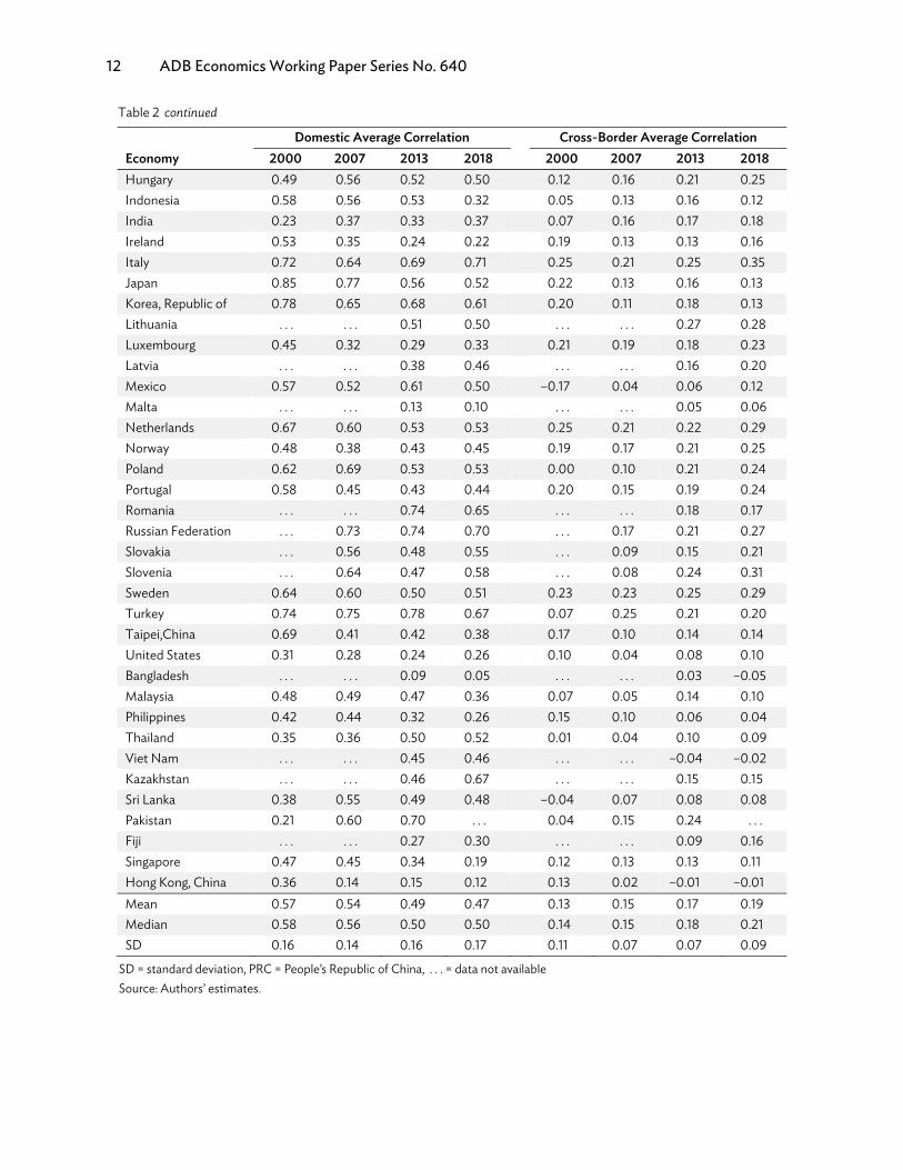
12 ADB Economics Working Paper Series No. 640
Domestic Average Correlation Cross-Border Average Correlation
Economy 2000 2007 2013 2018 2000 2007 2013 2018 Hungary 0.49 0.56 0.52 0.50 0.12 0.16 0.21 0.25 Indonesia 0.58 0.56 0.53 0.32 0.05 0.13 0.16 0.12 India 0.23 0.37 0.33 0.37 0.07 0.16 0.17 0.18 Ireland 0.53 0.35 0.24 0.22 0.19 0.13 0.13 0.16 Italy 0.72 0.64 0.69 0.71 0.25 0.21 0.25 0.35 Japan 0.85 0.77 0.56 0.52 0.22 0.13 0.16 0.13 Korea, Republic of 0.78 0.65 0.68 0.61 0.20 0.11 0.18 0.13 Lithuania . . . . . . 0.51 0.50 . . . . . . 0.27 0.28 Luxembourg 0.45 0.32 0.29 0.33 0.21 0.19 0.18 0.23 Latvia . . . . . . 0.38 0.46 . . . . . . 0.16 0.20 Mexico 0.57 0.52 0.61 0.50 –0.17 0.04 0.06 0.12 Malta . . . . . . 0.13 0.10 . . . . . . 0.05 0.06 Netherlands 0.67 0.60 0.53 0.53 0.25 0.21 0.22 0.29 Norway 0.48 0.38 0.43 0.45 0.19 0.17 0.21 0.25 Poland 0.62 0.69 0.53 0.53 0.00 0.10 0.21 0.24 Portugal 0.58 0.45 0.43 0.44 0.20 0.15 0.19 0.24 Romania . . . . . . 0.74 0.65 . . . . . . 0.18 0.17 Russian Federation . . . 0.73 0.74 0.70 . . . 0.17 0.21 0.27 Slovakia . . . 0.56 0.48 0.55 . . . 0.09 0.15 0.21 Slovenia . . . 0.64 0.47 0.58 . . . 0.08 0.24 0.31 Sweden 0.64 0.60 0.50 0.51 0.23 0.23 0.25 0.29 Turkey 0.74 0.75 0.78 0.67 0.07 0.25 0.21 0.20 Taipei,China 0.69 0.41 0.42 0.38 0.17 0.10 0.14 0.14 United States 0.31 0.28 0.24 0.26 0.10 0.04 0.08 0.10 Bangladesh . . . . . . 0.09 0.05 . . . . . . 0.03 –0.05 Malaysia 0.48 0.49 0.47 0.36 0.07 0.05 0.14 0.10 Philippines 0.42 0.44 0.32 0.26 0.15 0.10 0.06 0.04 Thailand 0.35 0.36 0.50 0.52 0.01 0.04 0.10 0.09 Viet Nam . . . . . . 0.45 0.46 . . . . . . –0.04 –0.02 Kazakhstan . . . . . . 0.46 0.67 . . . . . . 0.15 0.15 Sri Lanka 0.38 0.55 0.49 0.48 –0.04 0.07 0.08 0.08 Pakistan 0.21 0.60 0.70 . . . 0.04 0.15 0.24 . . . Fiji . . . . . . 0.27 0.30 . . . . . . 0.09 0.16 Singapore 0.47 0.45 0.34 0.19 0.12 0.13 0.13 0.11 Hong Kong, China 0.36 0.14 0.15 0.12 0.13 0.02 –0.01 –0.01 Mean 0.57 0.54 0.49 0.47 0.13 0.15 0.17 0.19 Median 0.58 0.56 0.50 0.50 0.14 0.15 0.18 0.21 SD 0.16 0.14 0.16 0.17 0.11 0.07 0.07 0.09
SD = standard deviation, PRC = People’s Republic of China, . . . = data not available Source: Authors’ estimates.
Table 2 continued

Credit Chain and Sectoral Comovement 13
IV. EMPIRICAL RESULTS
A. Base Results
With all variables constructed, our model specification is thus:
𝜌 = 𝜃 + 𝜂𝐺 + 𝛼 𝐶 + 𝛼 𝐶 + 𝛾𝑊 + 𝜖 , (26)
in which 𝑊 includes other determinants of sectoral correlation, and 𝐺 is the physical linkage between (𝑚, 𝑖) and (𝑚, 𝑖), which is computed as the first term in Eq. (13). We consider two fixed effects combinations: (1) economy fixed effects for input and output economies separately, and industry fixed effects for input and output industries separately, and (2) economy-industry joint fixed effects for input and output economy-industry pairs. We cluster standard errors based on the fixed effects combinations.
We present our results in models 1 to 4 of Table 3. Models (1) and (2) consider only an aggregate credit linkage (i.e., we do not separate the within and across economy credit linkages) for the two fixed effects combinations, and (3) and (4) consider the domestic and cross-border credit linkages, separately. In this specification, we use the 2018 MRIO table in computing the input-output linkage, and we compute the sectoral correlation using the prior 20 years INDSTAT and CPI data.
Table 3: Regression Table, 2018, Previous 20 Years
(1) (2) (3) (4) 𝜌 𝜌 𝜌 𝜌𝐺 0.781*** 0.784*** 0.759*** 0.736***
(0.0364) (0.0151) (0.0374) (0.0146) 𝐶 3.271∗∗ 3.342∗∗∗
(1.018) (0.461) 𝐶 6.050∗∗∗ 5.883∗∗∗
(1.138) (0.524) 𝐶 2.990∗∗ 2.880∗∗∗
(0.865) (0.456) Constant 0.185∗∗∗ 0.185∗∗∗ 0.186∗∗∗ 0.186∗∗∗ (0.000561) (0.000796) (0.000412) (0.000824) Economy 𝑚 FE yes no yes no Economy 𝑜 FE yes no yes no Industry 𝑖 FE yes no yes no Industry 𝑘 FE yes no yes no Economy-industry pair (𝑚, 𝑖) FE no yes no yes Economy-industry pair (𝑜, 𝑘) FE no yes no yes Observations 511,589 511,589 511,589 511,589 R2 0.226 0.427 0.227 0.428 Within R2 0.024 0.031 0.025 0.031
FE = fixed effects. Notes: Standard errors in parentheses and are robust to heteroskedasticity. *p <0.05, ** p <0.01, *** p <0.001. Source: Authors’ estimates.
14 ADB Economics Working Paper Series No. 640
Two observations are notable. First, we echo the results shown in Raddatz (2010); the significant and positive coefficient of 𝐶𝑖𝑘𝑚𝑜 in (1) and (2) support the hypothesis that the intensity of the use of trade credit increases the correlation between the two industries linked by the credit chain.
Second, we find that after separating the credit linkage, 𝐶𝑖𝑘𝑚𝑜, to the domestic component (or within economy linkage), 𝐶𝑖𝑘𝐷𝑚𝑜, and the cross-border component (or cross-border linkage), 𝐶 , the results remain similar in that the intensity of the use of trade credit still increases the correlation between the two industries, regardless of whether these two industries are in the same economy or different economies, as the coefficients of the two are positive and significant. Moreover, the comparison between the coefficients of 𝐶𝑖𝑘𝐷𝑚𝑜 and 𝐶𝑖𝑘𝐹𝑚𝑜 suggests that the domestic credit linkage has higher impact on the correlation between two industries within the same economy than that between two in two different economies.
B. Robustness
We note that one possible concern of the base specification is whether the results are robust to outliers. It could be possible that our results are driven by the strong correlations between a few strong economies and/or dominating industries. To address this concern, we follow two traditional approaches to reduce the effect of outliers: winsorization or trimming, the former is to set the extreme values of sectoral correlations (higher or lower than a certain threshold) to the value at the threshold, whereas the latter is to drop these extreme values from the sample.
We report the results of the above two robustness tests in Table A9. The first three columns are the results after winsorizing the sectoral correlation based on the top 1, 3, and 5 percentiles, and the last column shows the result after we trim the top 5% values. As we can observe from the coefficients of 𝐶 and 𝐶 , these two remain positive and significant, thereby, again, supporting our hypothesis that the intensity of the use of trade credit increases sectoral correlation. The magnitude of the two also suggests that the influence of domestic trade intensity is higher than that of cross-border one; although the extreme values indeed have impact on how much these trade intensity influences the correlation (as the gap between the two is slightly reduced), the impact is minor.
To further examine the outlier issues, we winsorize and trim our sample based on the respective percentile cutoffs based on the economy pairs instead of doing so for the entire sample and report the results in Table A10, and we again obtain qualitatively the same results.
C. Time Variation
In this section, we explore how the intensity of the use of trade credit influences sectoral correlation differently from 2000 to 2018. Specifically, we repeat the regression model in equation (26) but use the MRIO tables in year 2000, 2007, 2013, and 2018.17 In Table 4, we report our empirical results when the sectoral correlations are computed based on the prior 20 years of data.
17 Although the MRIO tables first started coverage in 2000, the next available table is conducted for 2007. Therefore, we pick the first two available tables in studying the time variation. The most updated table at the time of this study is conducted for 2018, and we find the middle year between 2007 and 2018 as another time span in our study, which is 2013.

Credit Chain and Sectoral Comovement 15
Table 4: Regression Table (Time Window: Previous 20 Years)
2000 2007 2013 2018 𝜌 𝜌 𝜌 𝜌𝐺 0.862*** 0.810*** 0.791*** 0.763***
(0.0184) (0.0122) (0.0126) (0.0146) 𝐶 12.12∗∗∗ 11.54∗∗∗ 7.842∗∗∗ 5.883∗∗∗ (1.175) (0.859) (0.667) (0.524) 𝐶 8.477∗∗∗ 5.015∗∗∗ 3.696∗∗∗ 2.880∗∗∗ (1.258) (0.899) (0.659) (0.456) Constant 0.123∗∗∗ 0.140∗∗∗ 0.163∗∗∗ 0.186∗∗∗ (0.00146) (0.00136) (0.000884) (0.000824) Economy-industry pair (𝑚, 𝑖) FE yes yes yes yes Economy-industry pair (𝑜, 𝑘) FE yes yes yes yes Observations 269,673 320,728 529,837 511,589 R2 0.347 0.275 0.329 0.428 Within R2 0.058 0.054 0.033 0.031
FE = fixed effects. Notes: Standard errors in parentheses and are robust to heteroskedasticity. *p <0.05, ** p <0.01, *** p <0.001. Source: Authors’ estimates.
We observe a decreasing trend of the positive relation between both the domestic and cross-border intensity of trade credit usage and correlations. First, while the coefficients of 𝐶 and 𝐶
remain significant and positive, the coefficient of 𝐶 changes from 12.12, to 11.54, to 7.842, to 5.883 and the coefficient of 𝐶 changes from 8.477, 5.015, 3.696, to 2.880 from 2000 to 2018. This decreasing trend suggests that the trade linkage intensity is gradually reducing its impact on sectoral correlations, regardless of the domestic or cross-border ones. We note that a similar pattern can be observed when we compute sectoral correlation based on the prior 10 years of data (see Table A11 for the results), except that using only 10 years of data, correlations tend to respond to a sudden change of pattern. Nonetheless, we still have a roughly decreasing trend, with a dip in 2013.
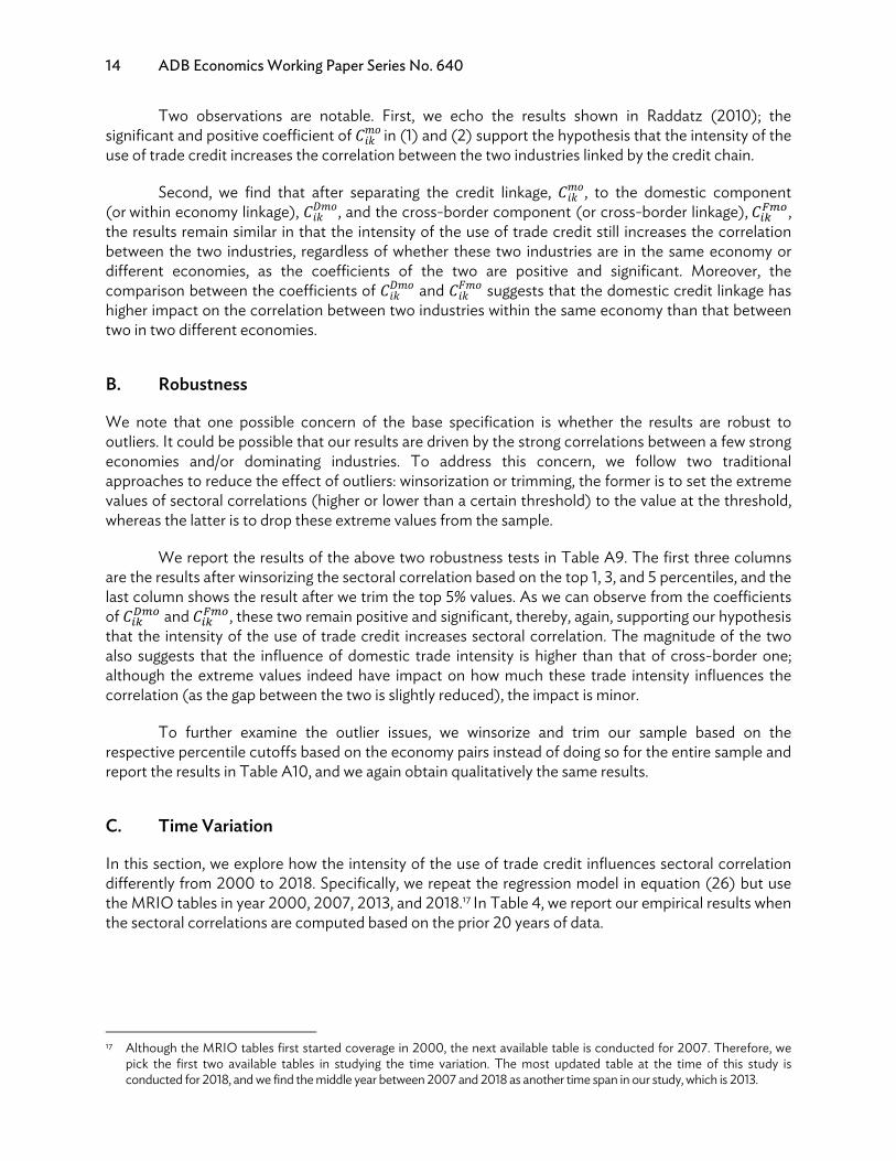
One plausible explanation is that the booming global trade credit linkages provide a risk diversification mechanism. We provide heatmaps of 𝐶 and 𝐶 for four economies: the People’s Republic of China, Japan, the Republic of Korea, and the US at years 2000 and 2018 in Figure 1. By comparing Figures 1(a) and 1(b), we observe that the intensity of the domestic use of trade credit declined during these 18 years; the diagonal values are colored by the intensity of the use of trade credit, and a more purple color refers to a higher intensity. On the other hand, by comparing Figures 1(c) and 1(d), we observe that the intensity of the cross-border use of trade credit increases during these 18 years; the off-diagonal values are colored by the intensity of the use of trade credit, and a more purple color refers to a higher intensity. From 2000 to 2018, production processes have been dissected into smaller and smaller, yet more and more specialized steps, thereby enabling international trades that are searching for cheap and high quality production sites/suppliers. As a result, trade credit linkages naturally have been diversified among different industries and/or different economies. With a more diversified credit linkage, the impact of certain shocks occurring in an industry thus plays a less important role, regardless of whether this trade credit linkage happens domestically or aboard.
We further support our argument using the domestic and cross-border trade share changes. See Figure 2 for the two plots as well as Table 5 for the summary statistics for the domestic trade share.
16 ADB Economics Working Paper Series No. 640
Figure 1: Heatmaps: CD and CFat 2000 and 2018, Time Window, Previous 20 Years
JPN = Japan, KOR = Republic of Korea, PRC = People's Republic of China, USA = United States. Source: Authors.
We find that in Figure 2(a), the domestic trade shares are shifting to the left when time increases, whereas in Figure 2(b), the cross-border trade shares are shifting to the right. A similar pattern can also be found in Table 5, in which the mean and the three percentiles are both decreasing throughout time. We note that although United Nations Conference on Trade and Development’s World Investment Report (UNCTAD 2020) finds that the level of the globalization of production continued to increase until 2010, then stagnated after that, our results on the share distributions on domestic and cross-border trades are still in a state of change over time (at least, fine-tuning the distribution of trades), even after 2010. This comparison also highlights the contribution of our analysis; while global trading volume has reached a steady state, the distribution has not, leading to a still-changing magnitude of sectoral comovement.

Credit Chain and Sectoral Comovement 17
Figure 2: Share of Domestic and Cross-Border Trade
Source: Authors.
Table 5: Summary Statistics of Domestic Trade Share
2000 2007 2013 2018 Mean 61.7 58.4 56.8 51.8 SD 21.1 20.4 21.6 23.7 25th percentile 51.1 44.9 38.9 34.9 50th percentile 63.9 55.5 56.0 50.5 75th percentile 76.5 76.5 74.6 71.6
SD = standard deviation. Source: Authors’ estimates.
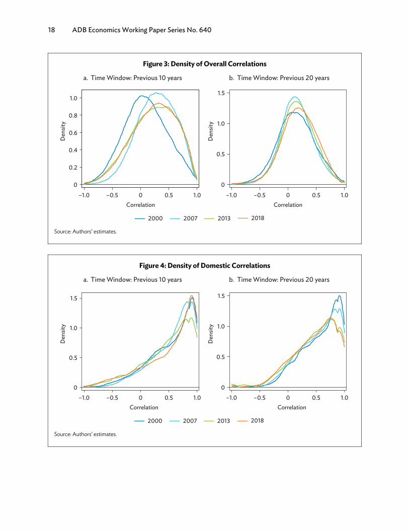
Another plausible explanation for the decreasing could be that global economies are gradually reducing their sectoral correlation by means of decoupling risks (e.g., better use of inventory management to buffer against uncertainties and shocks). To rule out this alternative, we plot overall correlations, the domestic correlations, and cross-border correlations in Figures 3–5, respectively, for a time window of the prior 10 years (a)18 and a time window of the prior 20 years (b). We also provide the summary statistics of these figures in Table 6.
Both the figures and the summary statistics reveal that comparing 2000 with 2018, while the overall correlation increases from 0.144 to 0.198, the domestic correlation decreases from 0.574 to 0.476 (use 20 years as our time window), whereas the cross-border correlation increases from 0.132 to 0.193.
18 As we previously mentioned, we can see that by using a 20-year time window, the density of correlations tends to be more
consistent throughout these 20 years, supporting our use of 20 years in our main specification and the reason the results in Table A11 tends to be volatile for the four time points.
18 ADB Economics Working Paper Series No. 640
Figure 3: Density of Overall Correlations
Source: Authors’ estimates.
Figure 4: Density of Domestic Correlations
Source: Authors’ estimates.
Credit Chain and Sectoral Comovement 19
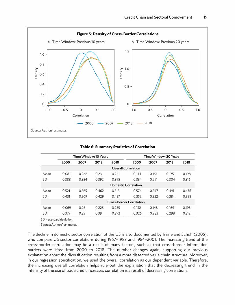
Figure 5: Density of Cross-Border Correlations
Source: Authors’ estimates.
Table 6: Summary Statistics of Correlation
Time Window: 10 Years Time Window: 20 Years
2000 2007 2013 2018 2000 2007 2013 2018 Overall Correlation Mean 0.081 0.268 0.23 0.241 0.144 0.157 0.175 0.198 SD 0.388 0.354 0.392 0.395 0.334 0.291 0.304 0.316 Domestic Correlation Mean 0.521 0.565 0.462 0.515 0.574 0.547 0.491 0.476 SD 0.431 0.369 0.429 0.437 0.352 0.352 0.384 0.388 Cross-Border Correlation Mean 0.069 0.26 0.225 0.235 0.132 0.148 0.169 0.193 SD 0.379 0.35 0.39 0.392 0.326 0.283 0.299 0.312
SD = standard deviation. Source: Authors’ estimates.
The decline in domestic sector correlation of the US is also documented by Irvine and Schuh (2005), who compare US sector correlations during 1967–1983 and 1984–2001. The increasing trend of the cross-border correlation may be a result of many factors, such as that cross-border information barriers were lifted from 2000 to 2018. The number changes again, supporting our previous explanation about the diversification resulting from a more dissected value chain structure. Moreover, in our regression specification, we used the overall correlation as our dependent variable. Therefore, the increasing overall correlation helps rule out the explanation that the decreasing trend in the intensity of the use of trade credit increases correlation is a result of decreasing correlations.
20 ADB Economics Working Paper Series No. 640
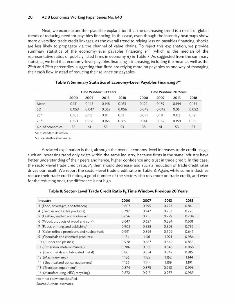
Next, we examine another plausible explanation that the decreasing trend is a result of global trends of reducing need for payables financing. In this case, even though the intensity heatmaps show more diversified trade credit linkages, as the overall trend to relying less on payables financing, shocks are less likely to propagate via the channel of value chains. To reject this explanation, we provide summary statistics of the economy-level payables financing 𝑃 (which is the median of the representative ratios of publicly listed firms in economy 𝑛) in Table 7. As suggested from the summary statistics, we find that economy-level payables financing is increasing, including the mean as well as the 25th and 75th percentiles, suggesting that firms are relying more on payables as one way of managing their cash flow, instead of reducing their reliance on payables.
Table 7: Summary Statistics of Economy-Level Payables Financing 𝑷𝒏
Time Window: 10 Years Time Window: 20 Years
2000 2007 2013 2018 2000 2007 2013 2018 Mean 0.131 0.145 0.148 0.163 0.122 0.139 0.144 0.154 SD 0.053 0.047 0.052 0.056 0.048 0.043 0.05 0.052 25th 0.103 0.115 0.111 0.13 0.091 0.111 0.112 0.121 75th 0.153 0.166 0.165 0.185 0.141 0.162 0.158 0.18 No. of economies 38 41 53 53 38 41 53 53
SD = standard deviation. Source: Authors’ estimates.
A related explanation is that, although the overall economy-level increases trade credit usage,
such an increasing trend only exists within the same industry, because firms in the same industry have better understanding of their peers and hence, higher confidence and trust in trade credit. In this case, the sector-level trade credit rate, 𝑃𝑗 then should decrease, and such a reduction of trade credit rates drives our result. We report the sector-level trade credit ratio in Table 8. Again, while some industries reduce their trade credit ratios, a good number of the sectors also rely more on trade credit, and even for the reducing ones, the difference is not high.
Table 8: Sector-Level Trade Credit Ratio Pj, Time Window: Previous 20 Years
Industry 2000 2007 2013 2018 3 (Food, beverages, and tobacco) 0.807 0.795 0.793 0.84 4 (Textiles and textile products) 0.797 0.747 0.752 0.728 5 (Leather, leather, and footwear) 0.656 0.715 0.729 0.704 6 (Wood, products of wood and cork) 0.647 0.627 0.584 0.601 7 (Paper, printing, and publishing) 0.902 0.838 0.803 0.786 8 (Coke, refined petroleum, and nuclear fuel) 0.991 0.896 0.709 0.647 9 (Chemicals and chemical products) 1.154 1.101 1.021 0.986 10 (Rubber and plastics) 0.928 0.887 0.849 0.855 11 (Other non-metallic mineral) 0.786 0.803 0.846 0.866 12 (Basic metals and fabricated metal) 0.86 0.854 0.842 0.815 13 (Machinery, nec) 1.156 1.129 1.152 1.144 14 (Electrical and optical equipment) 1.126 1.144 1.159 1.191 15 (Transport equipment) 0.874 0.875 0.910 0.996 16 (Manufacturing, NEC; recycling) 0.872 0.915 0.937 0.985
nec = not elsewhere classified. Source: Authors’ estimates.
Credit Chain and Sectoral Comovement 21
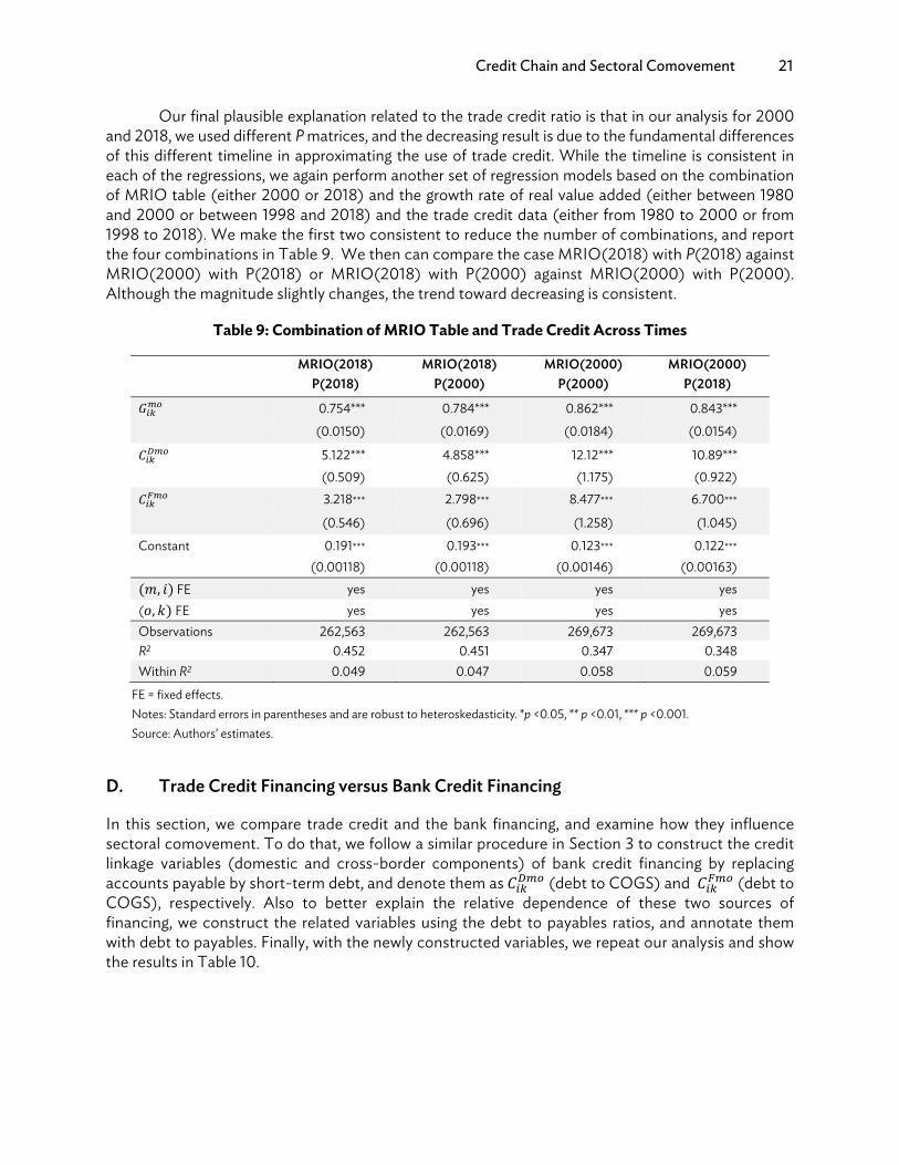
Our final plausible explanation related to the trade credit ratio is that in our analysis for 2000 and 2018, we used different P matrices, and the decreasing result is due to the fundamental differences of this different timeline in approximating the use of trade credit. While the timeline is consistent in each of the regressions, we again perform another set of regression models based on the combination of MRIO table (either 2000 or 2018) and the growth rate of real value added (either between 1980 and 2000 or between 1998 and 2018) and the trade credit data (either from 1980 to 2000 or from 1998 to 2018). We make the first two consistent to reduce the number of combinations, and report the four combinations in Table 9. We then can compare the case MRIO(2018) with P(2018) against MRIO(2000) with P(2018) or MRIO(2018) with P(2000) against MRIO(2000) with P(2000). Although the magnitude slightly changes, the trend toward decreasing is consistent.
Table 9: Combination of MRIO Table and Trade Credit Across Times
MRIO(2018) MRIO(2018) MRIO(2000) MRIO(2000) P(2018) P(2000) P(2000) P(2018) 𝐺 0.754*** 0.784*** 0.862*** 0.843***
(0.0150) (0.0169) (0.0184) (0.0154) 𝐶 5.122*** 4.858*** 12.12*** 10.89*** (0.509) (0.625) (1.175) (0.922) 𝐶 3.218∗∗∗ 2.798∗∗∗ 8.477∗∗∗ 6.700∗∗∗
(0.546) (0.696) (1.258) (1.045)
Constant 0.191∗∗∗ 0.193∗∗∗ 0.123∗∗∗ 0.122∗∗∗ (0.00118) (0.00118) (0.00146) (0.00163) (𝑚, 𝑖) FE yes yes yes yes (𝑜, 𝑘) FE yes yes yes yes Observations 262,563 262,563 269,673 269,673 R2 0.452 0.451 0.347 0.348 Within R2 0.049 0.047 0.058 0.059
FE = fixed effects. Notes: Standard errors in parentheses and are robust to heteroskedasticity. *p <0.05, ** p <0.01, *** p <0.001. Source: Authors’ estimates.
D. Trade Credit Financing versus Bank Credit Financing
In this section, we compare trade credit and the bank financing, and examine how they influence sectoral comovement. To do that, we follow a similar procedure in Section 3 to construct the credit linkage variables (domestic and cross-border components) of bank credit financing by replacing accounts payable by short-term debt, and denote them as 𝐶 (debt to COGS) and 𝐶 (debt to COGS), respectively. Also to better explain the relative dependence of these two sources of financing, we construct the related variables using the debt to payables ratios, and annotate them with debt to payables. Finally, with the newly constructed variables, we repeat our analysis and show the results in Table 10.
22 ADB Economics Working Paper Series No. 640
Table 10: Regression Table with Short-Term Debt, 2018, Previous 20 Years
(1) (2) (3) (4) (5) 𝜌 𝜌 𝜌 𝜌 𝜌 𝐺 0.785*** 0.851*** 0.787*** 0.871*** 0.784***
(0.0136) (0.0174) (0.0137) (0.0186) (0.0135) 𝐶 (payables to COGS) 5.681∗∗∗ 5.656∗∗∗ 5.235∗∗∗ (0.709) (0.934) (0.777) 𝐶 (payables to COGS) 2.678∗∗∗ 3.447∗∗∗ 2.914∗∗∗ (0.491) (0.697) (0.566) 𝐶 (debt to COGS) –1.370∗∗∗ –0.00124 (0.358) (0.397) 𝐶 (debt to COGS) –0.386∗ 0.465∗ (0.183) (0.225) 𝐶 (debt to payables) –0.115∗∗ –0.0365 (0.0379) (0.0292) 𝐶 (debt to payables) –0.0126 0.0231 (0.0155) (0.0141) Constant 0.187∗∗∗ 0.188∗∗∗ 0.187∗∗∗ 0.189∗∗∗ 0.187∗∗∗ (0.000813) (0.000650) (0.000791) (0.000513) (0.000787) Economy-industry pair (𝑚, 𝑖) FE yes yes yes yes yes Economy-industry pair (𝑜, 𝑘) FE yes yes yes yes yes Observations 511,589 511,589 511,589 511,589 511,589 R2 0.427 0.427 0.427 0.427 0.427 Within R2 0.031 0.0295 0.0307 0.0293 0.0307
COGS = cost of goods sold, FE = fixed effects. Notes: Standard errors in parentheses and are robust to heteroskedasticity. *p <0.05, ** p <0.01, *** p <0.001. We compute 𝐺 directly from the MRIO table, while Raddatz (2010) assumed that IO linkages in the US can be extrapolated to the rest of the economies, therefore, the effect of bank credit in our model might be different from that of the U.S. Source: Authors’ estimates.
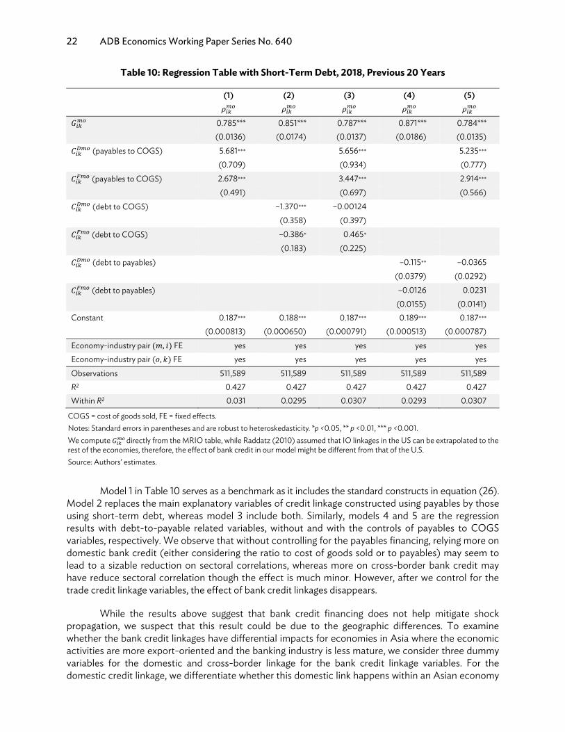
Model 1 in Table 10 serves as a benchmark as it includes the standard constructs in equation (26). Model 2 replaces the main explanatory variables of credit linkage constructed using payables by those using short-term debt, whereas model 3 include both. Similarly, models 4 and 5 are the regression results with debt-to-payable related variables, without and with the controls of payables to COGS variables, respectively. We observe that without controlling for the payables financing, relying more on domestic bank credit (either considering the ratio to cost of goods sold or to payables) may seem to lead to a sizable reduction on sectoral correlations, whereas more on cross-border bank credit may have reduce sectoral correlation though the effect is much minor. However, after we control for the trade credit linkage variables, the effect of bank credit linkages disappears.
While the results above suggest that bank credit financing does not help mitigate shock propagation, we suspect that this result could be due to the geographic differences. To examine whether the bank credit linkages have differential impacts for economies in Asia where the economic activities are more export-oriented and the banking industry is less mature, we consider three dummy variables for the domestic and cross-border linkage for the bank credit linkage variables. For the domestic credit linkage, we differentiate whether this domestic link happens within an Asian economy

Credit Chain and Sectoral Comovement 23
or not by considering an interaction term between 𝐶 with a dummy variable, Asia = 1 if m and o are both in Asia, and Asia = 0, otherwise. For the cross-border linkage, we include two interactions terms, 𝐶 × Either from Asia and 𝐶 × Both from Asia, in which the former refers to the case where m (exclusive) or o are in Asia, and the latter refers to the case where both m and o are in Asia. All 𝐶 and 𝐶 variable, if not noted, are based on the corresponding debt-related variables.
We report the results in Table 11. Models 1 to 3 refer to the result with the debt-to-COGS related variable without Asia related interaction terms, with Asia interaction terms, and finally with additional controls of payables-to-COGS related variables. Models 4 to 6 follow a similar order, except that we do so for debt-to-payables related variables. We observe two interesting results. First, when trading within Asia economies, regardless of domestic trades within an Asia economy or cross-border trades among Asia economies, relying more on bank credit than trade credit may help mitigate shock propagation, as the coefficients of 𝐶 × Asia and 𝐶 × Both from Asia in Models 5 and 6 are both negative and significant. Second, using more bank credit mitigates shock propagation for domestic trades in Asia, as the coefficients of 𝐶 × Asia are negative and significant in models 2 and 3.
Table 11: Regression Table with Short-Term Debt and Asia Interactions, 2018, Previous 20 Years
(1) (2) (3) (4) (5) (6) 𝜌 𝜌 𝜌 𝜌 𝜌 𝜌 𝐺 0.851*** 0.825*** 0.780*** 0.871*** 0.832*** 0.776***
(0.0174) (0.0164) (0.0131) (0.0186) (0.0176) (0.0129) 𝐶 (payables to COGS) 4.879∗∗∗ 4.391∗∗∗ (0.930) (0.794) 𝐶 (payables to COGS) 2.319∗∗ 1.801∗∗ (0.722) (0.616) 𝐶 (debt to COGS) –1.370∗∗∗ –0.769∗ 0.322 (0.358) (0.350) (0.373) 𝐶 (debt to COGS) –0.386∗ –0.357 0.0581 (0.183) (0.215) (0.254) 𝐶 (debt to payables) –0.115∗∗ –0.0564∗ –0.000873 (0.0379) (0.0270) (0.0215) 𝐶 (debt to payables) –0.0126 –0.00503 0.00605 (0.0155) (0.0175) (0.0182) 𝐶 × Asia –1.914∗∗∗ –1.423∗∗ –0.290∗∗∗ –0.212∗∗∗ (0.551) (0.531) (0.0654) (0.0637) 𝐶 × Either from Asia 1.703∗∗ 1.643∗∗ 0.0359 0.0292 (0.568) (0.558) (0.0493) (0.0476) 𝐶 × Both from Asia –1.844∗∗ –1.341 –0.508∗∗∗ –0.460∗∗∗ (0.699) (0.733) (0.0997) (0.0991) Constant 0.188∗∗∗ 0.189∗∗∗ 0.188∗∗∗ 0.189∗∗∗ 0.189∗∗∗ 0.187∗∗∗ (0.000650) (0.000526) (0.000761) (0.000513) (0.000429) (0.000778) Economy-industry pair (𝑚, 𝑖) FE
yes yes yes yes yes yes
Economy-industry pair (𝑜, 𝑘) FE
yes yes yes yes yes yes
continued on next page
24 ADB Economics Working Paper Series No. 640
(1) (2) (3) (4) (5) (6) 𝜌 𝜌 𝜌 𝜌 𝜌 𝜌
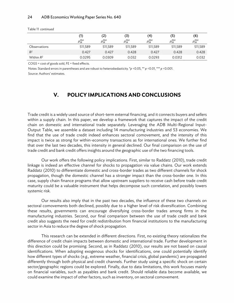
Observations 511,589 511,589 511,589 511,589 511,589 511,589 R2 0.427 0.427 0.428 0.427 0.428 0.428 Within R2 0.0295 0.0309 0.032 0.0293 0.0312 0.032
COGS = cost of goods sold, FE = fixed effects. Notes: Standard errors in parentheses and are robust to heteroskedasticity. *p <0.05, ** p <0.01, *** p <0.001. Source: Authors’ estimates.
V. POLICY IMPLICATIONS AND CONCLUSIONS
Trade credit is a widely used source of short-term external financing, and it connects buyers and sellers within a supply chain. In this paper, we develop a framework that captures the impact of the credit chain on domestic and international trade separately. Leveraging the ADB Multi-Regional Input-Output Table, we assemble a dataset including 14 manufacturing industries and 53 economies. We find that the use of trade credit indeed enhances sectoral comovement, and the intensity of this impact is twice as strong for within-economy transactions as for international ones. We further find that over the last two decades, this intensity in general declined. Our final comparison on the use of trade credit and bank credit offers insights around the geographic use of the two financing tools.
Our work offers the following policy implications. First, similar to Raddatz (2010), trade credit linkage is indeed an effective channel for shocks to propagation via value chains. Our work extends Raddatz (2010) to differentiate domestic and cross-border trades as two different channels for shock propagation, though the domestic channel has a stronger impact than the cross-border one. In this case, supply chain finance programs that allow upstream suppliers to receive cash before trade credit maturity could be a valuable instrument that helps decompose such correlation, and possibly lowers systemic risk.
Our results also imply that in the past two decades, the influence of these two channels on sectoral comovements both declined, possibly due to a higher level of risk diversification. Combining these results, governments can encourage diversifying cross-border trades among firms in the manufacturing industries. Second, our final comparison between the use of trade credit and bank credit also suggests the need for credit redistribution from financial institutions to the manufacturing sector in Asia to reduce the degree of shock propagation.
This research can be extended in different directions. First, no existing theory rationalizes the difference of credit chain impacts between domestic and international trade. Further development in this direction could be promising. Second, as in Raddatz (2010), our results are not based on causal identifications. When adopting exogenous shocks for identifications, one could potentially identify how different types of shocks (e.g., extreme weather, financial crisis, global pandemic) are propagated differently through both physical and credit channels. Further study using a specific shock on certain sector/geographic regions could be explored. Finally, due to data limitations, this work focuses mainly on financial variables, such as payables and bank credit. Should reliable data become available, we could examine the impact of other factors, such as inventory, on sectoral comovement.
Table 11 continued
REFERENCES
Babich, Vologymyr, and Christopher S. Tang. 2012. “Managing Opportunistic Supplier Product Adulteration: Deferred Payments, Inspection, and Combined Mechanisms.” Manufacturing & Service Operations Management 14 (2): 301–14.
Barrot, Jean-Noel. 2016. “Trade Credit and Industry Dynamics: Evidence from Trucking Firms. The Journal of Finance 71 (5): 1975–2016, ISSN 1540-6261.
Boissay, Frederic 2006. “Credit Chains and the Propagation of Financial Distress.” ECB Working Paper No. 573.
Boissay, Frederic, and Reint Gropp. 2013. “Payment Defaults and Interfirm Liquidity Provision.” Review of Finance 17 (6):1853–94.
Brennan, Michael, Vojislav Miksimovic, and Josef Zechner. 1988. “Vendor Financing.” Journal of Finance 43 (5): 1127–41.
Breza, Emily, and Andres Liberman. 2017. “Financial Contracting and Organizational Form: Evidence from the Regulation of Trade Credit.” Journal of Finance 72 (1): 291–324.
Burkart, Mike, and Torre Ellingsen. 2004. “In-Kind Finance: A Theory of Trade Credit.” American Economic Review 94 (3): 569–90.
Cardoso-Lecourtois, Miguel. 2004. “Chain Reactions, Trade Credit and the Business Cycle.” Econometric Society.
Chen, Christopher, Nitish Jain, and S. Alex Yang. 2020. “The Impact of Trade Credit Provision on Retail Inventory: An Empirical Investigation Using Synthetic Controls.” http://dx.doi.org/10.2139/ssrn.3375922.
Chod, Jiri, Evgeny Lyandres, and S. Alex Yang. 2019. “Trade Credit and Supplier Competition.” Journal of Financial Economics 131 (2): 484–505.
Cooper, Russell, and John Haltiwanger. 1990. “Inventories and the Propagation of Sectoral Shocks.” The American Economic Review 80 (1): 170–90.
Cuñat, Vicente 2007. “Trade Credit: Suppliers as Debt Collectors and Insurance Providers.” Review of Financial Studies 20 (2): 491–527.
Federal Reserve Board. 2019. Financial Accounts of the United States (Second quarter 2019).
Fisman, Raymond, and Inessa Love. 2003. “Trade Credit, Financial Intermediary Development, and Industry Growth.” Journal of Finance 58 (1): 353–74.
Giannetti, Mariassunta, Mike Burkart, and Tore Ellingsen. 2011. “What You Sell Is What You Lend? Explaining Trade Credit Contracts.” Review of Financial Studies 24 (4): 1261–98.

26 References
Irvine, Owen, and Scott D. Schuh. 2005. “The Roles of Co-Movement and Inventory Investment in the Reduction of Output Volatility.” Federal Reserve Bank of Boston Working Paper No. 05-9.
Jacobson, Tor, and Erik Von Schedvin. 2015. “Trade Credit and the Propagation of Corporate Failure: An Empirical Analysis.” Econometrica 83 (4): 1315–71.
Kiyotaki, Nobuhiro, and John Moore. 1998. “Credit Chains.” London School of Economics. Unpublished.
Kouvelis, Pano, and Wenhui Zhao. 2012. “Financing the Newsvendor: Supplier vs. Bank, and the Structure of Optimal Trade Credit Contracts.” Operations Research 60 (3): 566–80.
Lee, Hsiao-Hui, Jianer Zhou, and Jingqi Wang. 2018. “Trade Credit Financing Under Competition and Its Impact on Firm Performance in Supply Chains.” Manufacturing & Service Operations Management 20 (1): 36–52.
Lilien, David. 1982. “Sectoral Shifts and Cyclical Unemployment.” Journal of Political Economy 90 (4): 777–93.
Long, Michael, Ileen Malitz, and S. Abraham Ravid. 1993. “Trade Credit, Quality Guarantees, and Product Marketability.” Financial Management 117–27.
Long, Jr. John B., Charles I. Plosser. 1983. “Real Business Cycles.” Journal of political Economy 91 (1): 39–69.
Lucas, Robert E. 1995. “Understanding Business Cycles.” Essential Readings in Economics: 306–27.
McMillan, John, and Christopher Woodruff. 1999. “Interfirm Relationships and Informal Credit in Vietnam.” Quarterly Journal of Economics 114 (4): 1285–1320.
Miller, Ronald E., and Perter D. Blair. 2009. Input-Output Analysis: Foundations and Extensions. Cambridge: Cambridge University Press.
Nadiri, M. Ishaq. 1969 “The Determinants of Trade Credit in the US Total Manufacturing Sector.” Econometrica: Journal of the Econometric Society 37 (3): 408-23.
Ng, Chee, Janet Kiholm Smith, and Raghuram Smith. 1999. “Evidence on the Determinants of Credit Terms Used in Interfirm Trade.” Journal of Finance 54 (3): 1109–29.
Petersen, Mitchell, and Raghuram Rajan. 1997. “Trade Credit: Theories and Evidence”. Review of Financial Studies 10 (3): 661–91.
Peura, Heikki, S. Alex Yang, and Guoming Lai. 2017. “Trade Credit in Competition: A Horizontal Benefit.” Manufacturing Service Operations Management 19 (2): 263–89.
Raddatz, Claudio E. 2010. “Credit Chains and Sectoral Co-Movement: Does the Use of Trade Credit Amplify Sectoral Shocks?” The Review of Economics and Statistics 92 (4): 985–1003.
Rajan, Raghuram, and Luigi Zingales. 1995. “What Do We Know About Capital Structure? Some Evidence From International Data.” Journal of Finance 50 (5): 1421–60.

References 27
Schwartz, Robert. 1974. “An Economic Model of Trade Credit.” Journal of Financial and Quantitative Analysis 9 (4): 643–57.
Shea, John. 2002. “Complementarities and Comovements.” Journal of Money, Credit and Banking 34 (2): 412–33.
United Nations Conference on Trade and Development (UNCTAD). 2020. World Investment Report. Geneva.
Yang, S. Alex, and John Birge. 2018. “Trade Credit, Risk Sharing, and Inventory Financing Portfolios.” Management Science 64 (8): 3667–89.
ASIAN DEVELOPMENT BANK6 ADB Avenue, Mandaluyong City1550 Metro Manila, Philippineswww.adb.org
Credit Chain and Sectoral Comovement: A Multi-Region Investigation
Global supply chains become increasingly interconnected via financial linkages such as trade credit, thereby resulting in comovement across different sectors and regions. This paper empirically examines the impact of trade credit usage on comovement between sectors within each economy and across economies separately. It finds that trade credit linkage is an influential channel for both domestic and cross-border shocks to propagate and create a more profound impact on industries around the globe. It also shows that the impact of the domestic credit chains on sectoral comovement is twice as strong as that of the international ones.
About the Asian Development Bank
ADB is committed to achieving a prosperous, inclusive, resilient, and sustainable Asia and the Pacific, while sustaining its efforts to eradicate extreme poverty. Established in 1966, it is owned by 68 members —49 from the region. Its main instruments for helping its developing member countries are policy dialogue, loans, equity investments, guarantees, grants, and technical assistance.