Board of Governors of the Federal Reserve System

International Finance Discussion Papers

Number 1306

December 2020

Common Trade Exposure and Business Cycle Comovement

Oscar Avila-Montealegre and Carter Mix

Please cite this paper as:Avila-Montealegre, Oscar and Carter Mix (2020). “Common Trade Exposure and BusinessCycle Comovement,” International Finance Discussion Papers 1306. Washington: Board ofGovernors of the Federal Reserve System, https://doi.org/10.17016/IFDP.2020.1306.

NOTE: International Finance Discussion Papers (IFDPs) are preliminary materials circulated to stimu-late discussion and critical comment. The analysis and conclusions set forth are those of the authors anddo not indicate concurrence by other members of the research staff or the Board of Governors. Referencesin publications to the International Finance Discussion Papers Series (other than acknowledgement) shouldbe cleared with the author(s) to protect the tentative character of these papers. Recent IFDPs are availableon the Web at www.federalreserve.gov/pubs/ifdp/. This paper can be downloaded without charge from theSocial Science Research Network electronic library at www.ssrn.com.

Common Trade Exposure and Business Cycle Comovement

Oscar Avila-Montealegre Carter Mix∗

Abstract: A large empirical literature has shown that countries that trade more with each

other have more correlated business cycles. We show that previous estimates of this relation-

ship are biased upward because they ignore common trade exposure to other countries. When

we account for common trade exposure to foreign business cycles, we find that (1) the effect of

bilateral trade on business cycle comovement falls by roughly 25 percent and (2) common expo-

sure is a significant driver of business cycle comovement. A standard international real business

cycle model is qualitatively consistent with these facts but fails to reproduce their magnitudes.

Past studies have used models that allow for productivity shock transmission through trade to

strengthen the relationship between trade and comovement. We find that productivity shock

transmission increases business cycle comovement largely because of a country-pair’s common

trade exposure to other countries rather than because of bilateral trade. When we allow for

stronger transmission between small open economies than other country-pairs, comovement

increases both from bilateral trade and common exposure, similar to the data.

Keywords: trade, business cycles, open economy macroeconomics

JEL Classification: F1, E32, F41, F44

∗We are thankful for comments from George Alessandria, Yan Bai, Dan Lu, and from audiences at Midwest

Macroeconomics Conference (2019), the Central Bank of Colombia, and the University of Rochester. The views

expressed in this paper are solely the responsibility of the authors and should not be interpreted as reflecting

the views of the Board of Governors or of any other person associated with the Federal Reserve System or the

Central Bank of Colombia

1 Introduction

A large literature starting with Frankel and Rose (1998) argues that countries that trade more

with each other have more correlated business cycles – a phenomenon known as trade comove-

ment. But most studies ignore the countries’ common trade exposure to other trade partners,

which acts as an indirect source of business cycle comovement: If two countries are highly

exposed to a common partner, they face similar foreign shocks and comove more. We explore

the effects of bilateral trade and common trade exposure to foreign business cycles (common

exposure) on a country-pair’s business cycle comovement.

Our paper makes both empirical and theoretical contributions. Empirically, we docu-

ment two facts: (1) Omitting common exposure from the analysis biases the estimated trade-

comovement relation upward, and (2) bilateral trade and common trade exposure are both

important sources of business cycle comovement. The total effect of trade on business cycle

comovement, which includes effects from both bilateral trade and common trade exposure, is

much larger than reported in studies that exclude the common exposure channel. Theoretically,

we show that attempts to reconcile trade-comovement and standard international models by

allowing productivity shocks to be passed on to other countries through trade actually work

through the indirect channel of common exposure to third parties rather than through bilateral

trade.

As an illustrative example of the key empirical issue, consider Mexico and Canada.

Between 1990 and 2016 bilateral trade between Mexico and Canada accounted for less than

3 percent of their total trade, but their trade with the United States over the same period

accounted for almost 70 percent of their total trade. Consistent with the trade-comovement

relation in the empirical literature, measures of gross domestic product (GDP) comovement

between Canada and the United States and Mexico and the United States are high – 0.8 and

0.57, respectively – by our measure. As a result, GDP comovement between Canada and Mexico

is also high, about 0.4, even though they trade little with each other. Ignoring Canada and

Mexico’s common exposure to the United States would lead us to overestimate the effect of

their bilateral trade on comovement.

A simple ordinary least squares (OLS) regression confirms that country-pairs with

higher bilateral trade and common exposure to foreign cycles exhibit greater business cycle

comovement. To get the causal effect of bilateral trade on output comovement, we follow Frankel

1

and Rose (1998) and instrument trade using gravity determinants such as distance, common

language, and so on. To get the causal effect of common exposure on output comovement, we

restrict our sample to use only country-pairs of small open economies (SOEs), for which the

cycle of their trading partners is exogenous. For this sample, increasing bilateral trade by one

standard deviation raises output comovement by 2.9 percentage points (p.p.) while increasing

common exposure by one standard deviation raises output comovement by 4.0 p.p. We call the

additional comovement coming from common exposure trade-partner comovement as it often

results from exposure to similar countries. Omitting common exposure from the regression

raises the estimated effect of bilateral trade on business cycle comovement by roughly a third.

Kose and Yi (2001) show that a standard three-country international real business

cycle (IRBC) model exhibits much smaller – but still positive – trade comovement than we

see in the data. We expand upon their work by using a four -country IRBC model, which

can be calibrated to match both bilateral trade intensity and trade-partner similarity between

any two countries, and show that the model is once again qualitatively consistent with the

empirical facts but cannot reproduce their magnitudes. The failure of the model to reproduce

the magnitude of trade-partner-comovement is a new puzzle in the literature. This failure arises

because SOEs are subject to large idiosyncratic total factor productivity (TFP) shocks in the

baseline calibration. With smaller idiosyncratic shocks, each country’s business cycle is more

strongly affected by its trading partners and countries equally exposed to third parties have

higher comovement.

Kose and Yi (2006) show that if TFP shocks are more correlated as trade increases, the

model can produce trade comovement that is closer to the data. Following this result, other

researchers have tried to endogenize TFP transmission through trade and have had success

increasing trade comovement.1 We include exogenous TFP transmission through trade in our

model and show that the resulting increase in output comovement actually works through

the country-pair’s common exposure to other countries rather than through bilateral trade;

estimated trade-partner comovement gets much closer to its value in the data than does trade

comovement. Correlated TFP shocks solve the trade-partner-comovement puzzle but not the

trade-comovement puzzle.

TFP transmission fails to increase trade comovement because bilateral trade between

1See the next section for more details.

2

most countries is small compared with their total trade, so TFP transmission from the rest

of the world (ROW) far outweighs TFP transmission from any one trading partner. If two

countries trade with similar third parties, then TFP transmission increases their comovement

mostly from this channel. Because countries that trade more with each other also trade with

similar partners, the effect is misinterpreted as an increase in trade comovement when common

exposure is excluded from the analysis.

Our results suggest that a theory that explains trade comovement will need new

mechanisms beyond TFP transmission through trade. For our limited analysis of SOEs, scaling

up TFP transmission between SOEs compared with transmission between other country-pairs

can solve both puzzles as even small differences in bilateral trade intensities between SOE

country-pairs yield stronger TFP transmission. This solution keeps the model close to the

standard IRBC model with TFP shocks, but other shocks or mechanisms may also increase

business cycle transmission from bilateral trade.

In section 2, we present a brief literature review. Section 3 reports the empirical

results for the trade- and trade-partner-comovement relations. In section 4, we describe the

multi-country model. We report the calibration technique and the quantitative results in section

5. Section 6 concludes.

2 Related Literature

Using data for 20 industrialized economies, Frankel and Rose (1998) find that increasing trade

intensity by one standard deviation raises output comovement by 13 p.p. For a broader set of

countries and a longer period, Calderon et al. (2007) find a positive but smaller effect of bilateral

trade on output comovement: Increasing bilateral trade by one standard deviation raises output

comovement by between 2 and 8 p.p. Other studies that support the positive relation between

trade and business cycle comovement are Canova and Dellas (1993), Imbs (2000), Clark and

Van Wincoop (2001), Otto et al. (2001), Imbs (2004), Baxter and Kouparitsas (2005), Doyle

and Faust (2005) and Blonigen et al. (2014). The results in our paper confirm that bilateral

trade intensity is a key driver of business cycle comovement, but out paper also explores the

indirect channel of common trade exposure to foreign business cycles. In that sense, our paper

is closely related to de Soyres and Gaillard (2020), who show that similarity in trade networks

3

increases business cycle comovement. Their paper complements our empirical results. Our

paper explores how a standard IRBC model can be reconciled to these facts.

From a theoretical perspective, Kose and Yi (2001) assess whether the standard IRBC

framework can replicate the trade-comovement relation. The authors extend the Backus et al.

(1992) and Backus et al. (1994) model to include three countries and endogenous transportation

costs. They simulate a drop in trade costs that raises goods market integration and analyze

its effects on output synchronization. They find, as we do, that the model is qualitatively

consistent with the trade-comovement relation but fails to reproduce its magnitude. This

failure, known as the trade-comovement puzzle, has motivated a growing theoretical literature.

Kose and Yi (2006) show that with correlated productivity shocks the model is able to alleviate

the puzzle, and many researchers have since tried to endogenize this channel by modeling

multiple sectors and stages (see Ambler et al. (2002), Burstein et al. (2008), Arkolakis and

Ramanarayanan (2009), and Johnson (2014)). Johnson (2014) shows that with correlated

productivity shocks, the model generates a strong trade-comovement relation in the goods

sector but zero correlations for services and, thus, low aggregate correlations. From a micro

perspective, di Giovanni et al. (2018) document that trade and multinational linkages are

important sources of output correlations between a firm and a particular country. Cravino

and Levchenko (2016), who show that multinational firms contribute to the transmission of

shocks across countries, reinforce this evidence. The presence of multinationals and vertical

integration provide empirical evidence that may justify the inclusion of more correlated shocks

in standard IRBC models. Our paper shows that while all these mechanisms may help to

increase comovement, they are more likely to do so through a country-pair’s common exposure

to other countries rather than through bilateral trade.

Lowering the trade elasticity has also been shown to strengthen the trade-comovement

relation, as in Heathcote and Perri (2002), Kose and Yi (2006), and Burstein et al. (2008), but is

not enough to solve the puzzle. Drozd et al. (2020) show that modeling the disconnect between

the low short and the high long run trade elasticity is a promising avenue in resolving the

trade-comovement puzzle. We will perform all of our theoretical analyses using two different

trade elasticities from the literature.

4

3 Data and Empirical Analysis

Estimating the trade-comovement and trade-partner-comovement relations requires information

on bilateral trade flows and GDP. Feenstra et al. (2005) provides nominal bilateral imports

in US dollars, and the World Development Indicators (WDI) from the World Bank includes

information on GDP and its components in nominal and real terms. Following the trade-

comovement literature, we also gather information on economic development, trade openness,

and population, which is also available in the WDI. The Centre d’Etudes Prospectives Et

d’Informations Internationales (CEPII) database provides information on gravity determinants

such as distance, common language, colony relations, and geographic characteristics. The final

set of variables includes bilateral trade agreements from the Economic Integration Agreement

Data Sheet. Most of the information is available at the annual level since 1962. To get a

balanced panel with a richer set of countries, we focus on the period from 1990 to 2016.

3.1 Indicators

For the empirical exercise, we define three indicators: business cycle (or output) comovement,

bilateral trade intensity, and common exposure to foreign cycles. Output comovement for two

countries is defined as the correlation between the cyclical component of their annual real GDP

from 1990 to 2016 (∆GDPit), as in equation 1.

Comovi,j = Corr(∆GDPit,∆GDPjt). (1)

We use the method presented in Hamilton (2018) to get the cyclical component of

GDP at the business cycle frequency. Namely, ∆GDPi,t+2 is the estimated residual of the

regression

lnGDPit = β0 + β1 lnGDPi,t−2 + εit,

performed separately for each country.

Frankel and Rose (1998) measure bilateral trade intensity both as the ratio between

bilateral trade and the sum of the nominal GDP (equation 2) or as the ratio between bilateral

trade and total trade (equation 3)

TIGDPi,j =Xi,j +Mi,j +Xj,i +Mj,i

Yi + Yj(2)

5

TI tradei,j =Xi,j +Mi,j +Xj,i +Mj,i

Xi +Mi +Xj +Mj

, (3)

where Xi,j and Mi,j are exports and imports from country i to country j, respectively, and

Xi and Mi are total exports and imports of country i.2 In the empirical analysis, we use the

average trade intensities from 1990 to 2016.

To measure common exposure, we first calculate the trade-partner cycle of each coun-

try as the weighted average of the cycle of its trading partners, equation 4. Each trading

partner’s cycle is weighted by the country’s share of trade with that partner in 1990. We

calculate common exposure to foreign business cycles for countries i and j as the correlation

between their trade-partner cycles, equation 5.

TPCi =∑n

si,n∆GDPn (4)

si,n =Xi,n,1990 +Mi,n,1990

Xi,1990 +Mi,1990

ComovTPCi,j = Corr(TPCi, TPCj) (5)

We also use an indicator that measures trade-partner similarity and that is highly

correlated with common trade exposure to calibrate the model. To measure similarity, we

calculate the fraction of country i‘s total trade with each country n— si,n from above. For two

countries i and j, trade partner similarity TPSi,j is the sum of the absolute differences of the

trade shares si,n and sj,n for each country n 6= i, j as in equation 6. The TPS measure takes

values between 0 and 2. A TPS of 0 indicates identical trade shares with all external partners

(high similarity), and a TPS of 2 indicates that none of i’s trading partners trade with j and

vice versa (low similarity). By construction, countries with more similar trading partners (a

lower TPS value) will also have higher common trade exposure to foreign cycles.

TPSi,j =∑n 6=j,i

|si,n − sj,n| (6)

2Bilateral export and import data from both countries are used. Reported exports and imports between two

countries tend to differ because imports generally include freight and insurance costs and because of statistical

error. By including both countries’ data, our measure essentially takes the average of the reported exports and

imports in each country.

6

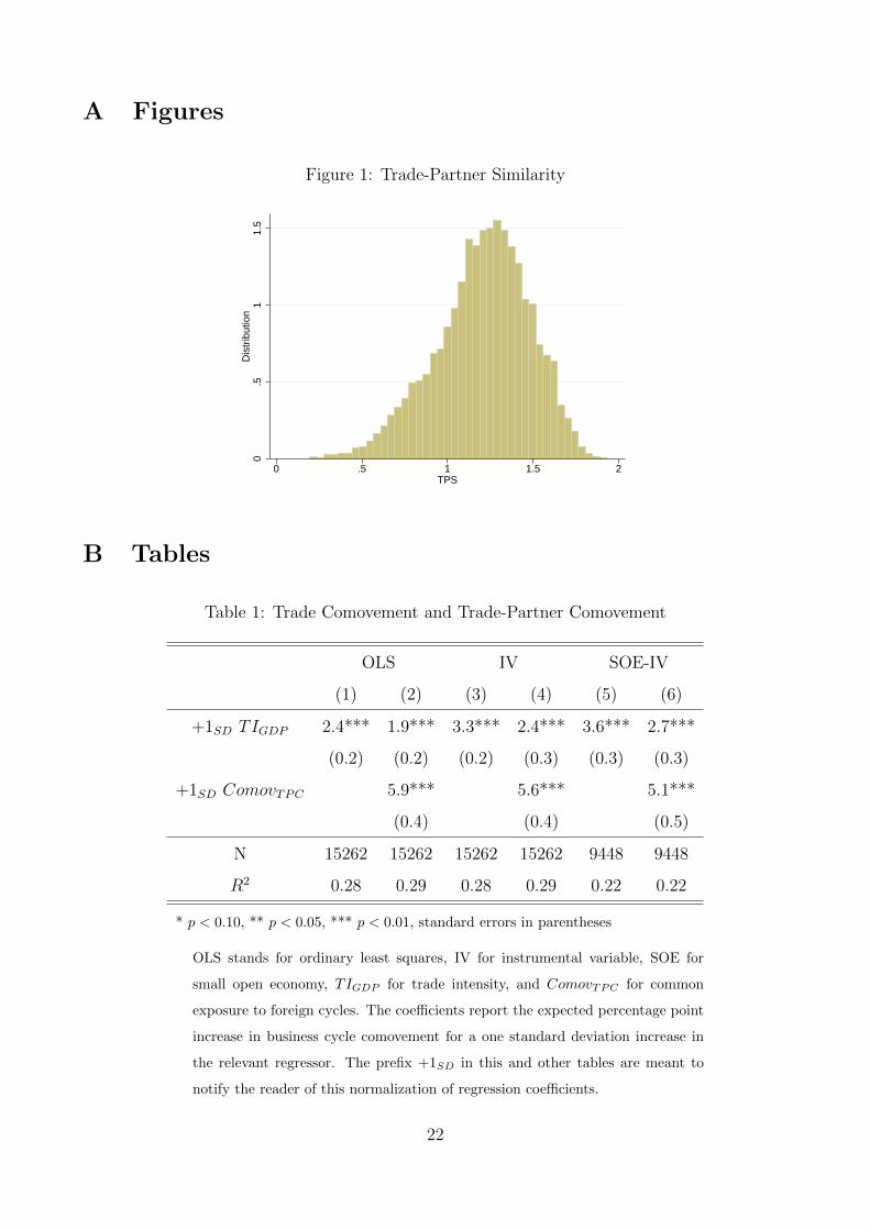
Figure 1 plots the distribution of TPS for a sample of more than 10,000 country-

pairs in 1990. On average, TPS takes a value of 1.23. Country-pairs that are close to the

mean are France and Costa Rica and Angola and Burkina Faso. Mexico and Canada have

the most similar trade partners (TPS = 0.20), while Saint Kitts and Nevis Islands and Yemen

have the least similar (TPS = 1.93). Other country-pairs with similar trade partners include

Dominican Republic and Mexico, Costa Rica and Honduras, Guatemala and Salvador, Sweden

and Denmark, Japan and South Korea, and France and Italy, all of which have a TPS below

0.3. Clearly, country-pairs with the lowest levels of TPS tend to be close geographically, just

as country-pairs with higher bilateral trade tend to be closer.3

3.2 Trade Comovement

Consider a simple empirical relationship between comovement and trade intensity:

Comovi,j = α1TIgdpi,j + αi + αj + α2Zi,j + vi,j (7)

where αi, αj are country fixed effects and Zi,j includes interactions for levels of development

and trade agreements. The residual is vi,j.

We estimate this relationship using OLS. Column 1 of Table 1 reports the standard-

ized coefficient for trade intensity. As expected, there is a positive and significant correlation

between bilateral trade and output synchronization. As Frankel and Rose (1998) highlight,

trade intensity and business cycle comovement are endogenously determined. On the one

hand, countries that trade more with each other may be subject to similar disturbances and

the transmission of shocks between countries may be stronger. On the other hand, economies

that are more synchronized may have more incentives to boost their trade. To get the causal

effect of trade intensity on output comovement, Frankel and Rose (1998) instrument bilateral

trade using gravity determinants. Here, we follow a similar approach and instrument trade

intensity by estimating the following equation:

TIgdpi,j = β0 + β1Xi + β2Xj + β3Xi,j + εi,j (8)

where Xi, Xj include country-specific characteristics such as population, latitude, longitude,

area, and an indicator for being landlocked, and Xi,j include bilateral distance in kilometers

3The relationship between distance and TPS is explored more fully in Appendix C.

7

and indicators for common language, common border, colony relations, and common region.

Table 2 reports the results for the OLS regression for equation 8. As in other studies, gravity

determinants have significant explanatory power on bilateral trade intensity. In a second stage,

we estimate the trade-comovement relation:

Comovi,j = α1T Igdp

i,j + αi + αj + α2Zi,j + vi,j (9)

where T Igdp

i,j is the predicted level of trade intensity and the rest of the variables are defined as in

equation 7. Column 3 of table 1 reports the regression results for equation 9. As in the simple

OLS, there is a positive and significant relation between trade intensity and business cycle

comovement: Increasing bilateral trade by one standard deviation raises output comovement

by 3.3 p.p.

3.3 Trade Comovement and Trade-Partner Comovement

We extend equation 7 to include common trade exposure as an additional control. Two out-

comes are expected. First, common exposure should increase output comovement. Second, the

effect of bilateral trade should fall as countries with more similar trade partners also tend to

have higher bilateral trade, meaning that some of the effect of common trade partners was being

captured by bilateral trade in the trade-comovement regressions from the previous section. In

other words, the trade-comovement relation is upward biased because common exposure is an

omitted variable. The new estimating equation (shown here as the second-stage regression) is

Comovi,j = α1T Igdp

i,j + γComovTPCi,j + αi + αj + α2Zi,j + vi,j (10)

Table 1 reports the estimated coefficients of bilateral trade and common exposure. In

all cases, the coefficients are standardized to facilitate interpretation. Columns 1 and 2 are

the results from a simple OLS regression, and columns 3 and 4 are those from instrumenting

bilateral trade, as in equation 8. Adding common exposure as an additional control reduces

the effect of bilateral trade by between 20 and 30 percent. The effect of common exposure

is positive and significant, meaning that common trade partners are an important source of

business cycle comovement. Finally, the combined effect of bilateral trade and common trade

exposure on output comovement is much larger than the isolated effect of bilateral trade in

8

regressions that exclude common exposure; trade has a larger effect on output comovement

than previously thought.

To get the causal effect of common exposure on output comovement, we focus on

small open economy (SOE) country-pairs. A SOE is unlikely to affect the business cycle of

its trading partners so the common exposure between two SOEs is exogenous to their business

cycle comovement. This exogeneity does not hold for a big country like the United States. The

United States affects the business cycles of Mexico and many of their common trade partners

so common exposure to foreign business cycles is not exogenous to output comovement between

Mexico and the United States. We define SOE country-pairs as pairs in which both countries

have a share of the world GDP less than 0.5 percent in 1990 and for which the pair’s bilateral

trade share is less than 10 percent. The latter assumption ensures that one SOE does not affect

the trade-partner cycle of the other.

The Columns 5 and 6 of Table 1 report the regression results when including only

SOE country-pairs. Consistent with the previous cases, including common exposure lowers the

effect of bilateral trade about 25 percent. Increasing trade intensity by one standard deviation

raises output comovement by 2.7 pp, while increasing common exposure raises comovement by

5.1 pp. Once again, the combined effect of trade on output comovement is larger than reported

in previous studies that ignore common trade exposure.

Our results are robust to using different methods of detrending GDP data (HP filter,

growth rates, band-pass filter), performing the analysis over different periods, using various

weighting schemes to estimate foreign business cycles, excluding the 2007-09 global recession,

using additional controls, and accounting for intra-industry trade. For details see Appendix D.

4 Model

Kose and Yi (2001) showed that an IRBC model could not reproduce the size of trade-

comovement seen in the data, and Kose and Yi (2006) modified the model to include correlated

TFP with transmission through trade to alleviate the trade-comovement puzzle. In this section,

we show that the IRBC model is also inconsistent with the trade-partner-comovement puzzle.

As in Kose and Yi (2006), correlated TFP increases business cycle comovement, but we show

that the increase comes mostly through a country-pair’s common exposure to other countries

9

and not directly through higher bilateral trade.

The model is close to the set-up proposed by Kose and Yi (2006) but with four

countries and constant iceberg costs (meaning that there is no role for a transportation sector).

Each economy produces one differentiated intermediate good that can be traded subject to

an iceberg cost τ . That is, for every unit of domestic goods that arrives in a foreign market,

the home country sends τ > 1 units of the good. Domestic capital and labor are combined

to produce intermediate goods in each country, and foreign and domestic intermediates are

aggregated to produce non-traded investment and consumption final goods. As in Heathcote

and Perri (2002), countries cannot trade financial assets.

4.1 Households

Each country has a representative consumer that chooses consumption Ci,t, leisure 1 − Li,t,

investment Ii,t, and physical capital Ki,t+1 to maximize lifetime utility over consumption and

leisure subject to a budget constraint. We assume investment is subject to adjustment costs.

The country i consumer’s problem is

U(Ci,t, Li,t) = max∞∑t=0

βt[Cµ

it(1− Li,t)1−µ]1−γ

1− γ(11)

subject to

P ci,t (Ci,t + Ii,t) = wi,tLi,t + ri,tKi,t (12)

Ki,t+1 = Ii,t + (1− δ)Ki,t −φk,i2

(Ii,tKi,t

− δ)2

(13)

where µ is the relative preference for consumption in the intratemporal utility, β is the discount

factor, 1/γ is the intertemporal elasticity of substitution, and φk,i determines the adjustment

costs for capital. wi, ri, andPci are the prices of labor, capital, and consumption and investment.

Each household has a fixed endowment of labor normalized to 1.

4.2 Intermediate Goods and Transportation Costs

Intermediate goods are produced by competitive firms that use capital and labor. Each country

produces a differentiated good traded in both domestic and foreign markets. The problem of

the representative firm in country i is to maximize profits by choosing capital and labor:

10

maxKi,t,Li,t

P xi,tYi,t − ri,tKi,t − wi,tLi,t (14)

P xi,t is the free-on-board or factory gate price of the intermediate good produced in

country i, and Yi,t is the production of the intermediate good in country i, which is represented

by a Cobb-Douglas production function with a constant capital share α and TFP zi,t, equation

15. TFP follows an auto-retrogressive process as in equation 16,

Yi,t = zi,tKαi,tL

1−αi,t (15)

log(zi,t) = (1− ρz)log(zi,ss) + ρzlog(zi,t) + εi,t (16)

where ρz ∈ (0, 1), zi,ss is the steady state value for the TFP, and εi,t is a normally distributed

random variable with mean zero and variance σ2i .

The market clearing condition in each period for producers of intermediate goods in

country i is:

Yi,t =N∑j

Yij,t. (17)

When the intermediate goods are exported to another country, they are subject to

an iceberg cost. The optimal price of an intermediate good produced in country i and sent to

country j is Pi,j = τi,jPxi where τi,j is the iceberg cost.

4.3 Final Goods

Competitive firms in the final goods sectors combine domestic and foreign intermediates to

produce non-traded consumption and investment goods. The firms in country i maximize

profits given by equation 18:

max{Xji,t}

P ci,t

(∑j

ω1/σji X

σ−1σ

ji,t

) σσ−1

−∑j

Pji,tXji,t (18)

where σ is the elasticity of substitution between home and foreign intermediates and ωij are

Armington weights that determine how important domestic and foreign varieties are for the

production of final goods (home-bias). Finally, the market clearing condition for the final goods

is given by

Ci,t + Ii,t =

(∑j

ω1/σji X

σ−1σ

ji,t

) σσ−1

. (19)

11

4.4 Competitive Equilibrium

Under financial autarky, a competitive equilibrium is a set of prices {P ci,t, wi,t, ri,t, P

xi,t, Pji,t}i,j

and allocations {Ci,t, Ki,t+1, Li,t+1, Ii,t+1, Yi,t, Yij,t, Xij,t}i,j such that for the exogenous produc-

tivity process zi,ti the following conditions hold:

• Given prices {P ci,t, wi,t, ri,t}i, consumers maximize their utility by choosing

{Ci,t, Li,t, Ki,t+1, Ii,t}i subject to their budget constraint and the capital law of motion.

• Given prices {P xi,t, ri,t, wi,t}i, intermediate goods producer maximize profits by choosing

{Ki,t, Li,t}i.

• Given prices {P ci,t, P

xji,t}i,j, final goods producers maximize profits by choosing {Xji,t}i,j.

• Labor, intermediate goods, and final goods markets clear.

5 Calibration and Simulations

5.1 Calibration

The model is calibrated to reproduce the empirical distributions of trade intensity and trade

partner similarity in SOEs, and to target some average moments in the data, such as the relative

size of SOEs and the trade openness in SOEs and the ROW. The data consist of 99 SOEs (4,725

unique country pairs). To reduce the scale of the model, we assume there are four countries,

two small and two ROW, and perform the calibration and simulation exercises 4,725 times.

Most of the parameters are taken directly from Kose and Yi (2006) and are reported in Table

3. Consistent with the Penn World Tables (PWTs), the productivity levels are normalized to

1.0 in the two SOEs and set to 1.5 in the ROWs.

We present our results with two different elasticities of substitution, σ = 1.5 and

σ = 0.7. The higher elasticity is typical in other business cycle studies such as Backus et al.

(1992) and Kose and Yi (2006), while Heathcote and Perri (2002) and Kose and Yi (2001) show

that a lower elasticity yields more business cycle comovement because foreign goods are more

complementary to domestic production.

The rest of the parameters, the 12 Armington weights, determine bilateral trade be-

tween all countries. Assuming that the SOEs and the ROWs are symmetric in some ways

12

reduces the number of parameters to six. Specifically, we assume that home bias is the same in

both SOEs, ωSOE1,SOE1 = ωSOE2,SOE2 , and in the two ROWs, ωROW1,ROW1 = ωROW2,ROW2 . Sim-

ilarly, we assume that the two SOEs are equally exposed to each other such that, ωSOE1,SOE2 =

ωSOE2,SOE1 , and that SOE1 is exposed to ROW1 the same way SOE2 is to ROW2, ωSOE1,ROW1 =

ωSOE2,ROW2 . Finally, we assume that ROW1 is exposed to SOE1 as ROW2 is to SOE2,

ωROW1,SOE1 = ωROW2,SOE2 , and that SOEs are similarly exposed to their opposite ROW,

ωSOE1,ROW2 = ωSOE2,ROW1 . For each country-pair in the data, the six remaining Armington

weights are calibrated to match

1. the bilateral trade intensity of the pair (both dividing by GDP and total trade, 2 moments)

2. trade partner similarity of the pair (1 moment)

3. average trade openness in SOEs and the ROW (2 moments)

4. average relative size between SOEs and the ROW (1 moment).

To make things simple, we carry out the calibration in two steps. First, we calibrate

the parameters to match the average moments from the data. Then, for each country pair we

re-calibrate the values of ωSOE1,SOE2 and ωSOE1,ROW1 to match the observed trade intensity and

trade partner similarity. Because recalibrating the Armington weights for each country is costly,

we only calculate the weights that correspond to the minimum and maximum values of trade

intensity and trade-partner similarity in the data. We then scale the weights for each country

pair according to its place in the distribution. Notice that if we had only three countries, as

in Kose and Yi (2006), we would be unable to match both bilateral trade intensity and trade

partner similarity.

Table 4 reports the targeted moments and their model counterpart for a country-pair

with average trade intensity and trade partner similarity; the model does well replicating the

data. For the pair-specific trade intensity and trade partner similarity, we report the root mean

square error (RMSE) for the model versus the data in the last two rows of Table 4. Again,

the model matches the data well. Table 5 reports the calibrated Armington weights for the

average country-pair. SOEs tend to rely on trade more than the ROW, as reflected in the lower

home bias (ωii). SOEs also trade less with each other, reflected in low values for the Armington

weight on goods from the other SOE. The Armington weights for goods produced in each of

13

the ROW countries replicates the trade partner similarity observed in the data. For the mean

country-pair, SOE1 is more exposed to ROW1, and SOE2 is more exposed to ROW2.

The calibration uses trade partner similarity rather than common exposure because

common exposure is determined endogenously in the model by fluctuations in GDP among the

country-pair’s trade partners. From a simple OLS regression of trade-partner-similarity (TPS)

on common exposure we find that that countries with more similar trading partners have more

common trade exposure to foreign cycles, as expected. The coefficient for this regression is

significant at the 1 percent level and equal to negative 0.31, with an R2 of 19 percent. The

advantage of the TPS is that it can be easily mapped into the model by changing the importance

of foreign intermediates in the production of domestic final goods.

The last set of parameters describes the productivity process in the intermediate goods

sector. Using the productivity levels reported in the PWTs we extract the cyclical component

of productivity and estimate a first-order auto-regressive process for each SOE, as in equation

20. The estimated persistence ρi,1 and standard deviation of the error term, σi, are used to

simulate the model. For the ROW, we assume that productivity behaves as in the United

States, and for the countries with no data in the PWTs, we use the mean process for SOEs.

TFP hpi,t = ρ0 + ρi,1TFP

hpi,t−1 + εi,t (20)

5.2 Simulations

For each country-pair the model is simulated for 1,000 periods and the last 27 are used to

calculate output comovement, common exposure, and other business cycle moments. As in the

data, GDP components are logged detrended using the method in Hamilton (2018). To get the

causal effect of bilateral trade on output comovement, we use the value of trade intensity in

the steady state. Using the 4,725 observations we estimate the trade-comovement and trade-

partner comovement relations, as in equation 10. Table 6 reports the estimated coefficients from

the simulations. Both coefficients are positive and significant, and adding common exposure

in the regression decreases the effect of trade intensity as in the data. However, the estimated

coefficients are much smaller than in the data. As noted by Table 7, another failure of the

model is the low volatility of GDP components.

The model gets the qualitative relations because trade transmits business cycle fluc-

14

tuations. As explained in Drozd et al. (2020), there are two forces that affect the trade-

comovement relationship: substitution and income effect. A positive productivity shock in the

foreign country increases the supply of the foreign intermediate and lowers its price. Since

the home country uses foreign intermediates to produce consumption and investment goods,

cheaper intermediates boosts the domestic production at home and increases the demand for

labor and investment, creating a positive relationship between trade and comovement. This

effect is the substitution effect and is stronger if home and foreign intermediates are less substi-

tutable. The income effect works in the opposite direction, a positive productivity shock abroad

creates a wealth effect at home by improving the terms of trade. Higher income reduces the

labor supply and has a negative effect on capital accumulation and production, which weakens

the link between trade and comovement. In the current model, the income effect is too strong

so that our trade-comovement coefficient is much smaller than in the data.

In addition to these two forces, our model with four countries has an additional source

of comovement if the two SOEs are similarly exposed to the larger countries. The common

exposure coefficient in the regression, however, is also much smaller than in the data. The

relation in the model is weak because idiosyncratic productivity shocks in SOEs are a major

source of SOE output fluctuations. If two countries had no productivity shocks and were

equally exposed to a third country, they would face the same forces and their output would

be highly correlated. Indeed, when we estimate the relations in a version of the model with

no productivity shocks in SOEs, we get a trade-partner-comovement coefficient more than six

times larger than in the data. Any modification that decreases the idiosyncratic volatility of

TFP shocks would therefore bring the model closer to the estimated trade-partner-comovement

from the data.

5.3 TFP Transmission and Trade Comovement

We modify our benchmark model to include correlated TFP shocks and countercyclical trade

barriers. Kose and Yi (2006) show that correlated TFP shocks increase the model’s ability

to match the estimated trade-comovement in the data. We find that while correlated shocks

do increase comovement, the increase comes primarily from the indirect channel of common

exposure to other countries.

We assume that a country’s productivity shock is partially transmitted to other coun-

15

tries and that the strength of transmission depends on how important a country is for its trading

partner, which is captured by the parameter ωij. The shock to TFP for country i at time t is

therefore

εi,t = εi,t + ν∑j 6=i

ωjiεj,t (21)

where εi,t are shocks that originate in country i. The parameter ν scales the impact of foreign

shocks. Previously, we had obtained the volatility of the TFP shock εi,t for countries in our

analysis. Now we solve for the volatilities of the new TFP shocks εi,t that guarantee that εi,t

has the same volatility as the data. The variance of εi,t is

σ2i = σ2

i + ν2∑j 6=i

ω2jiσ

2j

where εi,t has variance σ2i . The volatilities σ that solve the problem are

σ2 = A−1σ2

where

A = ν2

1ν2 ω2

21 ω231 ω2

41

ω212

1ν2 ω2

32 ω242

ω213 ω2

231ν2 ω2

43

ω214 ω2

24 ω234

1ν2

,

σ2 is

σ2 =

σ21

σ22

σ23

σ24

with σ2 similarly defined.

The correct volatilities can be solved for any value of ν. The larger is ν, the smaller

are the idiosyncratic volatilities σ for each country. Because large volatilities in SOEs caused

the low trade-partner comovement in the model, we choose ν to be its largest value that still

guarantees all variances remain nonnegative. For the high elasticity case, we get ν = 2.3.

For the low elasticity case, ν = 5.5. Though some country-specific volatilities are significantly

reduced, the standard deviation of the average SOE’s idiosyncratic shock falls by only between

5 and 7 percent.

16

To get more volatility in trade, we assume trade barriers (iceberg costs) are negatively

correlated with productivity shocks, as in equation 22. The parameters κi and κj are adjusted

to increase the volatility of exports and imports to be close to the volatility in the data. The

countercyclicality of trade barriers is consistent with a model in which a shipping industry with

finite cargo space chooses prices to maximize profits. When productivity is high, more goods

are being traded and the cost of shipping those goods increases.4

log(τij,t) = log(τij,ss)− (κiεi,t + κjεj,t) (22)

The model with countercyclical trade barriers has more volatility in investment and

trade flows as shown in column (3) of Table 7. Countercyclical barriers, however, do nothing to

improve or hinder trade- or trade-partner comovement; the coefficients from a model with only

correlated TFP shocks (not shown) are almost identical to those with correlated TFP shocks

and countercyclical barriers, which we discuss next.

Columns 5 and 6 of Table 6 report the coefficients for the trade-comovement and trade-

partner-comovement relations in the modified model. As in the benchmark case, increasing

trade intensity or common trade exposure has a positive effect on business cycle comovement.

With correlated productivity shocks (and the implied lower idiosyncratic volatilities in SOEs),

the trade-partner-comovement relation in the model is much closer to the data. The effect of

trade intensity, however, remains far below its value in the data.

When we exclude common exposure from the regression on model-simulated data,

the modified model shows much higher trade-comovement, moving from 0.3 to 1.5 in the high

elasticity model and from 0.5 to 1.3 in the low elasticity model, which accounts for 38 (1.5−0.33.5−0.3)

and 27 (1.3−0.53.5−0.5) percent of the discrepancy between the benchmark model and the data. Indeed,

this is the point of Kose and Yi (2006) and other models that endogenize TFP transmission.

But when we control for common exposure, the trade-comovement coefficient rises by much

less from the benchmark model and accounts for only 20 (0.6−0.12.6−0.1) and 21 (0.7−0.2

2.6−0.2) for the low

and high elasticity models. By contrast, the trade-partner-comovement coefficients in the new

model rise by much more, accounting for 77 and 41 percent of the discrepancy in trade-partner-

comovement between the benchmark model and the data. Therefore, TFP transmission through

trade mainly increases comovement through common foreign exposure rather than directly

4We could also get more volatility in trade by making trade intensive in capital goods. The results are

similar.

17

through bilateral trade, especially for the model with a higher elasticity.

The reason that TFP transmission works mainly through common exposure is that

the bilateral trade exposure between SOEs – and indeed between most country-pairs – is small

in comparison with exposure to the ROW. In our model, the parameter ωSOE1,SOE2 , which pins

down bilateral trade between the SOEs, are low in calibration (between 0 and 0.038). With

the correlated productivity shocks introduced earlier, shocks in one SOE have almost no direct

effect on the other SOE’s productivity, so the model fails to generate trade comovement directly

through bilateral trade. The values for ωSOEi,ROWiare bigger, so comovement between SOEs

increases if they have common exposure to the ROW countries. If we exclude common exposure

from the regression, this effect looks like an increase in comovement because of bilateral trade

because bilateral trade and common exposure are positively correlated.

Our results suggest that TFP transmission through trade mostly addresses the indirect

channel of trade and business cycle comovement. Attempts to solve the trade-comovement

puzzle in the literature will benefit from additional mechanisms that allow for stronger business

cycle transmission through bilateral trade rather than through common exposure to foreign

countries.

For example, one change we could make in our model is to assume that transmission

of productivity shocks between SOEs is higher than between other country pairs:

log(zi,t) = (1− ρz,i)log(zi,ss) + ρz,ilog(zi,t) + εi,t +∑j 6=i

νijωjiεj,t (23)

where νij is 10 times larger when both i and j are SOEs.5 One might justify such an assumption

by considering that SOEs with high bilateral trade are likely affected similarly by changes in

commodity prices, which can have a big influence on SOE cycles. To differentiate between the

two assumptions on correlated productivity, we call this one biased productivity shocks.

The coefficients for the trade-comovement and trade-partner-comovement relations

with biased productivity shocks are reported in columns 7 and 8 of Table 6. The trade-

comovement coefficient is now much closer to the data. With a higher elasticity, the trade-

comovement coefficient is 3.0 (versus 2.7 in the data) and the trade-partner-comovement coef-

ficient is 4.8 (versus 5.1 in the data). With a lower elasticity, the trade-comovement cofficient

is 3.7 and the trade-partner-comovement coefficient is 3.3. Other shocks or mechanisms may

5Once again, idiosyncratic volatilities are chosen to match the volatilities from the data and ν is selected to

guarantee nonnegative variance for all countries.

18

achieve a similar outcome, but this solution is meant (1) to preserve the IRBC structure with

TFP shocks in each country, and (2) to illustrate that scaling up the effect of bilateral trade

on business cycle transmission relative to the effect of common trade exposure is key to solving

the puzzles.

6 Conclusion

We argue that common trade exposure to foreign business cycles is an important source of

output comovement, especially in SOEs. Our empirical results suggest that measures of the

trade-comovement relation that omit common exposure are biased upward and that the total

effect of trade on output comovement is larger than previously thought due to common exposure.

On the theoretical side, we document that a standard international real business cycle model

is qualitatively consistent with the trade-comovement and trade-partner-comovement relations

but fails to replicate their magnitudes. Incorporating TFP transmission through trade increases

comovement but mostly through a country-pair’s common trade exposure to other countries

rather than through bilateral trade. A solution to the trade-comovement and trade-partner-

comovement puzzles needs therefore to scale up transmission of business cycles through bilateral

trade. We propose one solution to these puzzles that preserves the IRBC framework, but more

research must be done to endogenize transmission mechanisms that solve the puzzles. For

instance, SOEs that trade with higher bilateral trade or are in similar geographic areas are

subject to other common shocks (such as fluctuations in the terms of trade) that may increase

comovement.

References

Ambler, S., Cardia, E., and Zimmermann, C. (2002). International transmission of the business

cycle in a multi-sector model. European Economic Review, 46(2):273–300.

Arkolakis, C. and Ramanarayanan, A. (2009). Vertical specialization and international business

cycle synchronization. The Scandinavian Journal of Economics, 111(4):655–680.

Backus, D. K., Kehoe, P. J., and Kydland, F. E. (1992). International real business cycles.

Journal of Political Economy, 100(4):745–775.

19

Backus, D. K., Kehoe, P. J., and Kydland, F. E. (1994). Dynamics of the trade balance and

the terms of trade: The j-curve? The American Economic Review, 84(1):84–103.

Baxter, M. and King, R. G. (1999). Measuring business cycles: Approximate band-pass filters

for economic time series. Review of Economics and Statistics, 81(4):575–593.

Baxter, M. and Kouparitsas, M. A. (2005). Determinants of business cycle comovement: A

robust analysis. Journal of Monetary Economics, 52(1):113–157.

Blonigen, B. A., Piger, J., and Sly, N. (2014). Comovement in gdp trends and cycles among

trading partners. Journal of International Economics, 94(2):239–247.

Burstein, A., Kurz, C., and Tesar, L. (2008). Trade, production sharing, and the international

transmission of business cycles. Journal of Monetary Economics, 55(4):775–795.

Calderon, C., Chong, A., and Stein, E. (2007). Trade intensity and business cycle synchroniza-

tion: Are developing countries any different? Journal of International Economics, 71(1):2–21.

Canova, F. and Dellas, H. (1993). Trade interdependence and the international business cycle.

Journal of International Economics, 34(1–2):23–47.

Clark, T. E. and Van Wincoop, E. (2001). Borders and business cycles. Journal of International

Economics, 55(1):59–85.

Cravino, J. and Levchenko, A. A. (2016). Multinational firms and international business cycle

transmission. The Quarterly Journal of Economics, 132(2):921–962.

de Soyres, F. and Gaillard, A. (2020). Global trade and gdp co-movement. International

Finance Discussion Papers, 1282.

di Giovanni, J., Levchenko, A. A., and Mejean, I. (2018). The micro origins of international

business-cycle comovement. American Economic Review, 108(1):82–108.

Doyle, B. M. and Faust, J. (2005). Breaks in the variability and comovement of g-7 economic

growth. Review of Economics and Statistics, 87(4):721–740.

Drozd, L. A., Kolbin, S., Nosal, J. B., et al. (2020). The trade-comovement puzzle. American

Economic Journal: Macroeconomics, forthcoming.

20

Feenstra, R. C., Lipsey, R. E., Deng, H., Ma, A. C., and Mo, H. (2005). World trade flows:

1962-2000. Technical report, National Bureau of Economic Research.

Frankel, J. A. and Rose, A. K. (1998). The endogenity of the optimum currency area criteria.

The Economic Journal, 108(449):1009–1025.

Grubel, H. G. and Lloyd, P. J. (1971). The empirical measurement of intra-industry trade.

Economic Record, 47(4):494–517.

Hamilton, J. D. (2018). Why you should never use the hodrick-prescott filter. Review of

Economics and Statistics, 100(5):831–843.

Heathcote, J. and Perri, F. (2002). Financial autarky and international business cycles. Journal

of Monetary Economics, 49(3):601–627.

Imbs, J. (2000). Sectors and the OECD business cycle, volume 2473. Centre for Economic

Policy Research.

Imbs, J. (2004). Trade, finance, specialization, and synchronization. Review of Economics and

Statistics, 86(3):723–734.

Johnson, R. C. (2014). Trade in intermediate inputs and business cycle comovement. American

Economic Journal: Macroeconomics, 6(4):39–83.

Kose, M. A. and Yi, K.-M. (2001). International trade and business cycles: Is vertical special-

ization the missing link? American Economic Review, 91(2):371–375.

Kose, M. A. and Yi, K.-M. (2006). Can the standard international business cycle model explain

the relation between trade and comovement? Journal of international Economics, 68(2):267–

295.

Mendoza, E. G. (1995). The terms of trade, the real exchange rate, and economic fluctuations.

International Economic Review, 36(1):101–137.

Otto, G., Voss, G. M., and Willard, L. (2001). Understanding OECD output correlations.

Reserve Bank of Australia Sydney.

Schmitt-Grohe, S. and Uribe, M. (2018). How important are terms-of-trade shocks? Interna-

tional Economic Review, 59(1):85–111.

21

A Figures

Figure 1: Trade-Partner Similarity

0.5

11.

5D

istr

ibut

ion

0 .5 1 1.5 2TPS

B Tables

Table 1: Trade Comovement and Trade-Partner Comovement

OLS IV SOE-IV

(1) (2) (3) (4) (5) (6)

+1SD TIGDP 2.4*** 1.9*** 3.3*** 2.4*** 3.6*** 2.7***

(0.2) (0.2) (0.2) (0.3) (0.3) (0.3)

+1SD ComovTPC 5.9*** 5.6*** 5.1***

(0.4) (0.4) (0.5)

N 15262 15262 15262 15262 9448 9448

R2 0.28 0.29 0.28 0.29 0.22 0.22

* p < 0.10, ** p < 0.05, *** p < 0.01, standard errors in parentheses

OLS stands for ordinary least squares, IV for instrumental variable, SOE for

small open economy, TIGDP for trade intensity, and ComovTPC for common

exposure to foreign cycles. The coefficients report the expected percentage point

increase in business cycle comovement for a one standard deviation increase in

the relevant regressor. The prefix +1SD in this and other tables are meant to

notify the reader of this normalization of regression coefficients.

22

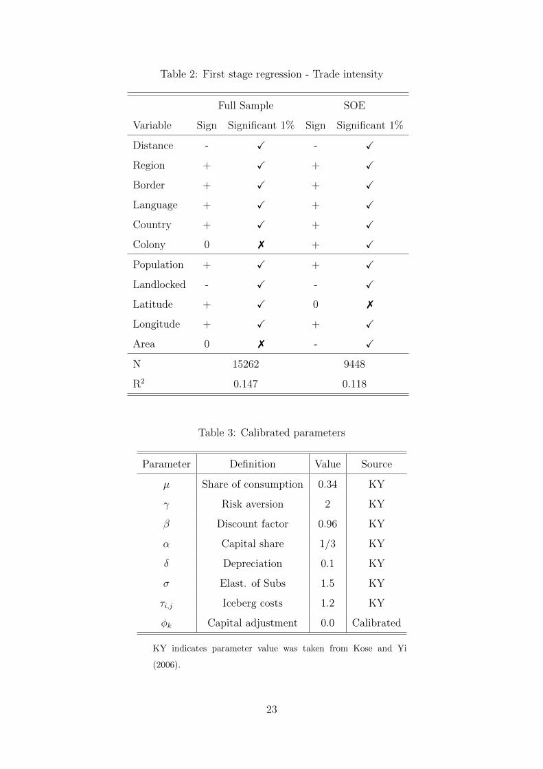
Table 2: First stage regression - Trade intensity

Full Sample SOE

Variable Sign Significant 1% Sign Significant 1%

Distance - X - X

Region + X + X

Border + X + X

Language + X + X

Country + X + X

Colony 0 7 + X

Population + X + X

Landlocked - X - X

Latitude + X 0 7

Longitude + X + X

Area 0 7 - X

N 15262 9448

R2 0.147 0.118

Table 3: Calibrated parameters

Parameter Definition Value Source

µ Share of consumption 0.34 KY

γ Risk aversion 2 KY

β Discount factor 0.96 KY

α Capital share 1/3 KY

δ Depreciation 0.1 KY

σ Elast. of Subs 1.5 KY

τi,j Iceberg costs 1.2 KY

φk Capital adjustment 0.0 Calibrated

KY indicates parameter value was taken from Kose and Yi

(2006).

23

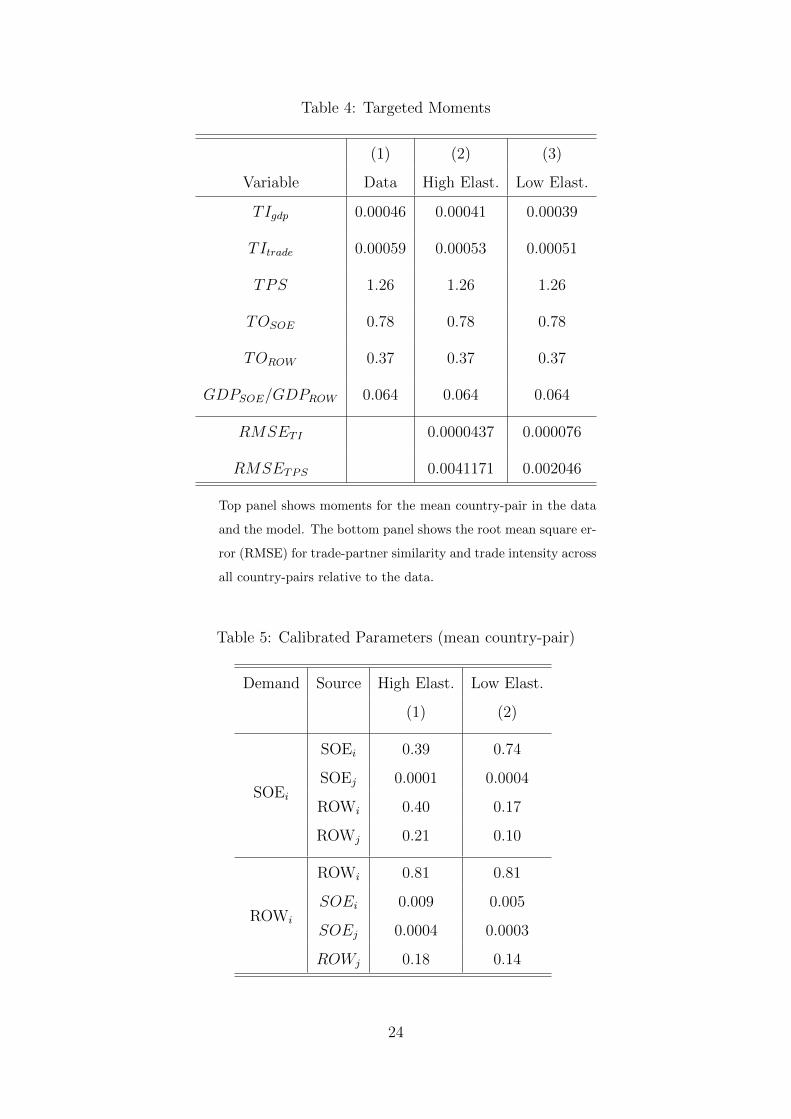
Table 4: Targeted Moments

(1) (2) (3)

Variable Data High Elast. Low Elast.

TIgdp 0.00046 0.00041 0.00039

TItrade 0.00059 0.00053 0.00051

TPS 1.26 1.26 1.26

TOSOE 0.78 0.78 0.78

TOROW 0.37 0.37 0.37

GDPSOE/GDPROW 0.064 0.064 0.064

RMSETI 0.0000437 0.000076

RMSETPS 0.0041171 0.002046

Top panel shows moments for the mean country-pair in the data

and the model. The bottom panel shows the root mean square er-

ror (RMSE) for trade-partner similarity and trade intensity across

all country-pairs relative to the data.

Table 5: Calibrated Parameters (mean country-pair)

Demand Source High Elast. Low Elast.

(1) (2)

SOEi

SOEi 0.39 0.74

SOEj 0.0001 0.0004

ROWi 0.40 0.17

ROWj 0.21 0.10

ROWi

ROWi 0.81 0.81

SOEi 0.009 0.005

SOEj 0.0004 0.0003

ROWj 0.18 0.14

24

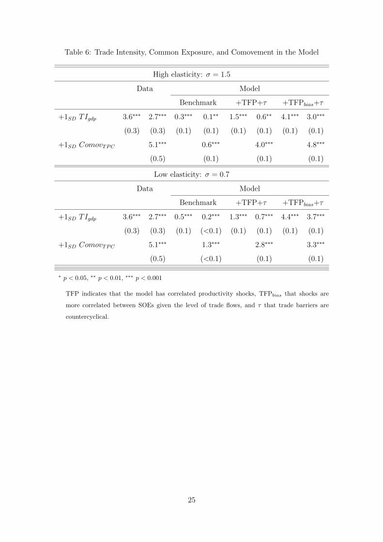
Table 6: Trade Intensity, Common Exposure, and Comovement in the Model

High elasticity: σ = 1.5

Data Model

Benchmark +TFP+τ +TFPbias+τ

+1SD TIgdp 3.6∗∗∗ 2.7∗∗∗ 0.3∗∗∗ 0.1∗∗ 1.5∗∗∗ 0.6∗∗ 4.1∗∗∗ 3.0∗∗∗

(0.3) (0.3) (0.1) (0.1) (0.1) (0.1) (0.1) (0.1)

+1SD ComovTPC 5.1∗∗∗ 0.6∗∗∗ 4.0∗∗∗ 4.8∗∗∗

(0.5) (0.1) (0.1) (0.1)

Low elasticity: σ = 0.7

Data Model

Benchmark +TFP+τ +TFPbias+τ

+1SD TIgdp 3.6∗∗∗ 2.7∗∗∗ 0.5∗∗∗ 0.2∗∗∗ 1.3∗∗∗ 0.7∗∗∗ 4.4∗∗∗ 3.7∗∗∗

(0.3) (0.3) (0.1) (<0.1) (0.1) (0.1) (0.1) (0.1)

+1SD ComovTPC 5.1∗∗∗ 1.3∗∗∗ 2.8∗∗∗ 3.3∗∗∗

(0.5) (<0.1) (0.1) (0.1)

∗ p < 0.05, ∗∗ p < 0.01, ∗∗∗ p < 0.001

TFP indicates that the model has correlated productivity shocks, TFPbias that shocks are

more correlated between SOEs given the level of trade flows, and τ that trade barriers are

countercyclical.

25

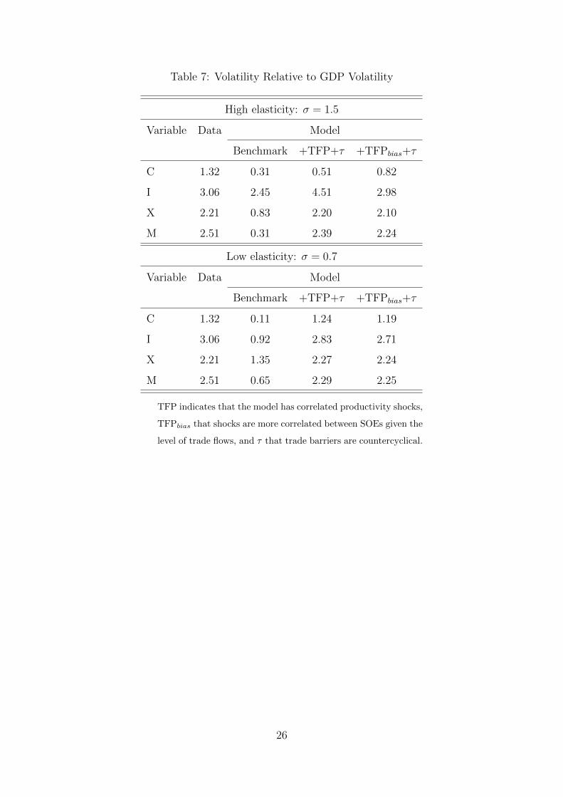
Table 7: Volatility Relative to GDP Volatility

High elasticity: σ = 1.5

Variable Data Model

Benchmark +TFP+τ +TFPbias+τ

C 1.32 0.31 0.51 0.82

I 3.06 2.45 4.51 2.98

X 2.21 0.83 2.20 2.10

M 2.51 0.31 2.39 2.24

Low elasticity: σ = 0.7

Variable Data Model

Benchmark +TFP+τ +TFPbias+τ

C 1.32 0.11 1.24 1.19

I 3.06 0.92 2.83 2.71

X 2.21 1.35 2.27 2.24

M 2.51 0.65 2.29 2.25

TFP indicates that the model has correlated productivity shocks,

TFPbias that shocks are more correlated between SOEs given the

level of trade flows, and τ that trade barriers are countercyclical.

26

C TPS and Distance

On average country-pairs, within the same continent have a lower TPS value than countries

in different regions, 1.01 versus 1.27. Columns (1) and (2) of table 8 report a simple OLS

regression between TPS and an indicator for common continent. It shows that country-pairs

in the same continent are more likely to have similar exposure to their trading partners. By

comparing the regions, we observe that Europe is the continent with the lowest TPS, 0.76,

while Africa is the one with the highest, 1.1. Not surprisingly, these results are consistent with

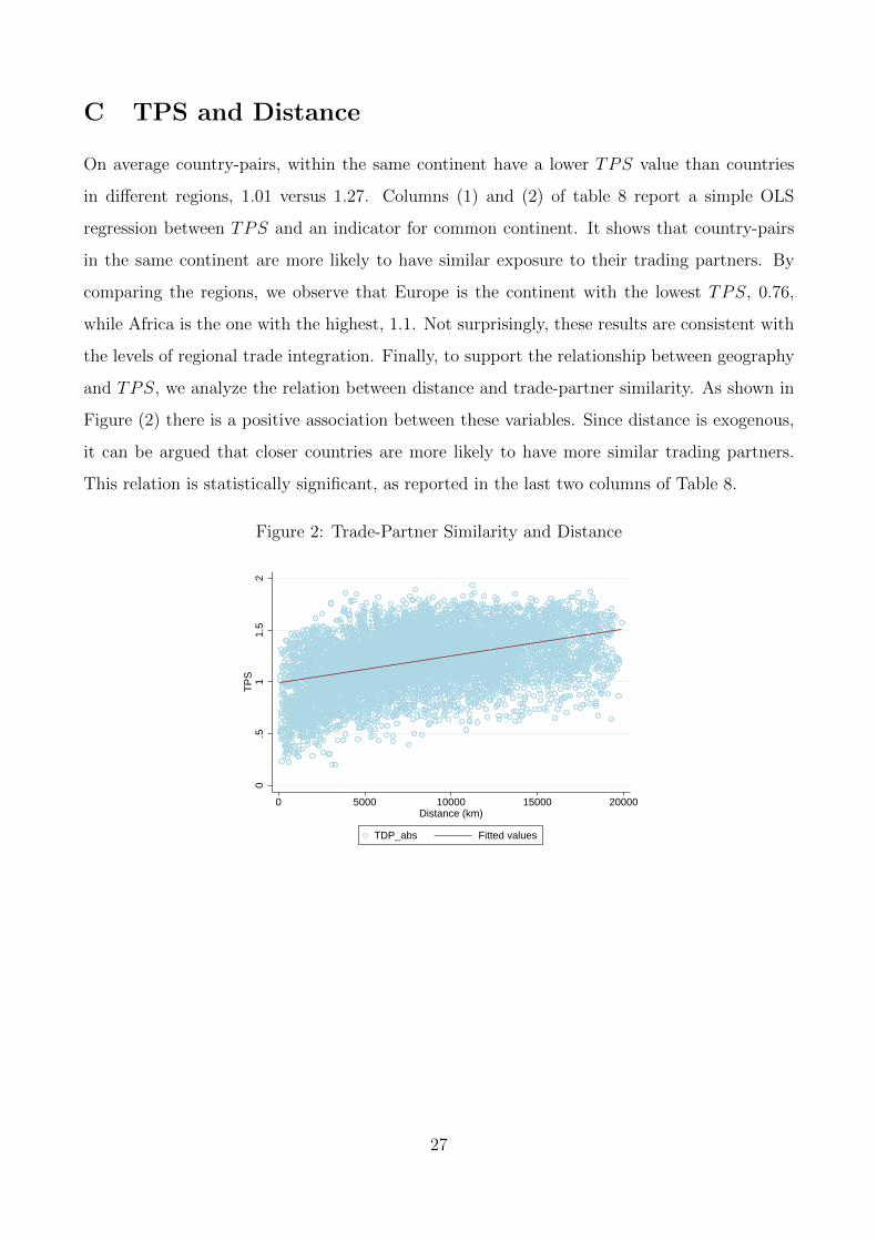
the levels of regional trade integration. Finally, to support the relationship between geography

and TPS, we analyze the relation between distance and trade-partner similarity. As shown in

Figure (2) there is a positive association between these variables. Since distance is exogenous,

it can be argued that closer countries are more likely to have more similar trading partners.

This relation is statistically significant, as reported in the last two columns of Table 8.

Figure 2: Trade-Partner Similarity and Distance

0.5

11.

52

TP

S

0 5000 10000 15000 20000Distance (km)

TDP_abs Fitted values

27

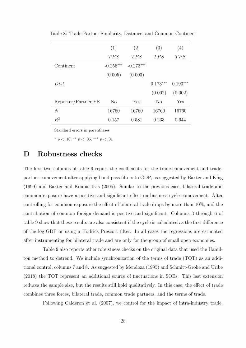
Table 8: Trade-Partner Similarity, Distance, and Common Continent

(1) (2) (3) (4)

TPS TPS TPS TPS

Continent -0.256∗∗∗ -0.273∗∗∗

(0.005) (0.003)

Dist 0.173∗∗∗ 0.193∗∗∗

(0.002) (0.002)

Reporter/Partner FE No Yes No Yes

N 16760 16760 16760 16760

R2 0.157 0.581 0.233 0.644

Standard errors in parentheses

∗ p < .10, ∗∗ p < .05, ∗∗∗ p < .01

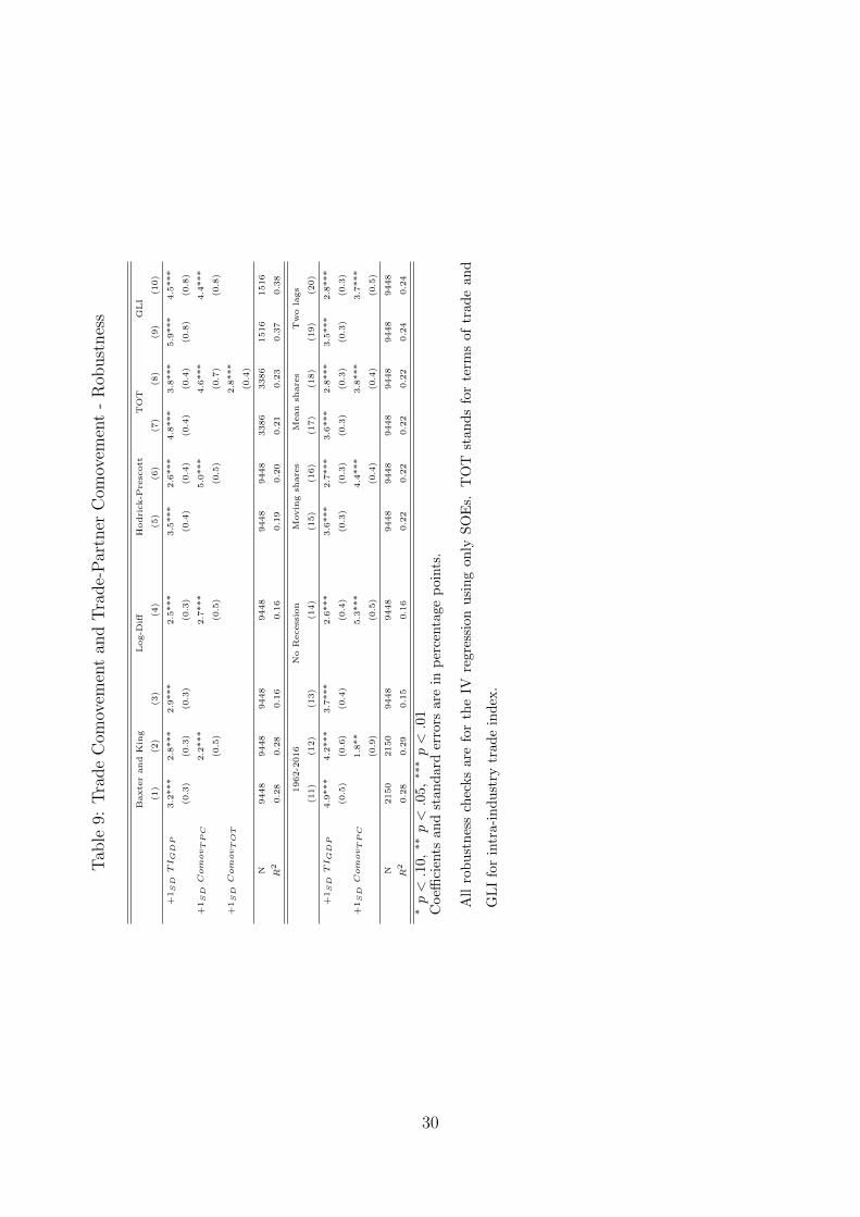
D Robustness checks

The first two columns of table 9 report the coefficients for the trade-comovement and trade-

partner comovement after applying band pass filters to GDP, as suggested by Baxter and King

(1999) and Baxter and Kouparitsas (2005). Similar to the previous case, bilateral trade and

common exposure have a positive and significant effect on business cycle comovement. After

controlling for common exposure the effect of bilateral trade drops by more than 10%, and the

contribution of common foreign demand is positive and significant. Columns 3 through 6 of

table 9 show that these results are also consistent if the cycle is calculated as the first difference

of the log-GDP or using a Hodrick-Prescott filter. In all cases the regressions are estimated

after instrumenting for bilateral trade and are only for the group of small open economies.

Table 9 also reports other robustness checks on the original data that used the Hamil-

ton method to detrend. We include synchronization of the terms of trade (TOT) as an addi-

tional control, columns 7 and 8. As suggested by Mendoza (1995) and Schmitt-Grohe and Uribe

(2018) the TOT represent an additional source of fluctuations in SOEs. This last extension

reduces the sample size, but the results still hold qualitatively. In this case, the effect of trade

combines three forces, bilateral trade, common trade partners, and the terms of trade.

Following Calderon et al. (2007), we control for the impact of intra-industry trade.

28

Grubel and Lloyd (1971) propose an indicator that measures if two countries are trading the

same kind of goods. Using a 4-Digit imports from Feenstra et al. (2005) we calculate the

following indicator for each country-pair:

GLIi,j = 1−

(∑k

|xki,j −mki,j|/

∑k

(xki,j +mki,j)

), (24)

where xki,j and mki,j are exports from country i to country j and imports from country i

to country j, respectively, and k represents the industry. Data are not available for all countries

and the sample size shrinks considerably for SOEs. Columns 9 and 10 of table 9 report the

coefficients for the trade-comovement and trade-partner comovement relations. As in previous

cases, both relations are positive and significant. Also, after controlling for common trade

partners the effect of bilateral trade falls.

Columns 11 and 12 (bottom panel) extend the time period from 1962 to 2016. This

extension reduces the size of the sample of SOEs by more than half but the results still hold.

Columns 13 and 14 show the results when GDP movements during the Global Financial Crisis

(2007-09) are not included. Columns 15 through 18 use various timing for the trade shares that

weight foreign GDP to get the trade partner cycle. Whether we use mean trade shares over the

whole sample or even changing trade shares over time, the results are the same. Finally, we

extend the Hamilton regression used to detrend the data to include an additional lag, columns

19 and 20. In all cases, the results hold.

29

Tab

le9:

Tra

de

Com

ovem

ent

and

Tra

de-

Par

tner

Com

ovem

ent

-R

obust

nes

s

Baxte

rand

Kin

gL

og-D

iffH

odri

ck-P

resc

ott

TO

TG

LI

(1)

(2)

(3)

(4)

(5)

(6)

(7)

(8)

(9)

(10)

+1SDTIG

DP

3.2

***

2.8

***

2.9

***

2.5

***

3.5

***

2.6

***

4.8

***

3.8

***

5.9

***

4.5

***

(0.3

)(0

.3)

(0.3

)(0

.3)

(0.4

)(0

.4)

(0.4

)(0

.4)

(0.8

)(0

.8)

+1SDComovT

PC

2.2

***

2.7

***

5.0

***

4.6

***

4.4

***

(0.5

)(0

.5)

(0.5

)(0

.7)

(0.8

)

+1SDComovT

OT

2.8

***

(0.4

)

N9448

9448

9448

9448

9448

9448

3386

3386

1516

1516

R2

0.2

80.2

80.1

60.1

60.1

90.2

00.2

10.2

30.3

70.3

8

1962-2

016

No

Recess

ion

Movin

gsh

are

sM

ean

share

sT

wo

lags

(11)

(12)

(13)

(14)

(15)

(16)

(17)

(18)

(19)

(20)

+1SDTIG

DP

4.9

***

4.2

***

3.7

***

2.6

***

3.6

***

2.7

***

3.6

***

2.8

***

3.5

***

2.8

***

(0.5

)(0

.6)

(0.4

)(0

.4)

(0.3

)(0

.3)

(0.3

)(0

.3)

(0.3

)(0

.3)

+1SDComovT

PC

1.8

**

5.3

***

4.4

***

3.8

***

3.7

***

(0.9

)(0

.5)

(0.4

)(0

.4)

(0.5

)

N2150

2150

9448

9448

9448

9448

9448

9448

9448

9448

R2

0.2

80.2

90.1

50.1

60.2

20.2

20.2

20.2

20.2

40.2

4

∗p<.1

0,∗∗p<.0

5,∗∗

∗p<.0

1C

oeffi

cien

tsan

dst

and

ard

erro

rsare

inp

erce

nta

ge

poin

ts.

All

rob

ust

nes

sch

ecks

are

for

the

IVre

gre

ssio

nu

sin

gon

lyS

OE

s.T

OT

stan

ds

for

term

sof

trad

ean

d

GL

Ifo

rin

tra-

ind

ust

rytr

ade

ind

ex.

30