Trade in Intermediate Inputsand Business Cycle Comovement

Robert C. Johnson∗

October 2010

PRELIMINARY AND INCOMPLETE.

Abstract

The standard international real business cycle model struggles to replicate thestrong empirical correlation between bilateral trade and output comovement. Thispaper explores whether trade in intermediate inputs resolves this puzzle. I integrateinput trade into a many country, multi-sector model, and calibrate the model to matchbilateral input-output linkages. I find that input trade fails to resolve the aggregatepuzzle. The model fails in large part because it cannot match the observed correlationof services output across countries. In contrast, the model matches observed corre-lations of goods output well. Further, independent shocks across countries explainone-quarter of the trade-comovement relationship for gross output of goods. However,because independent shocks are transmitted through input linkages, they synchronizegross output, not value added. Using simulated data, I argue that caution is needed ininterpreting trade-comovement regressions that include proxies for vertical linkages.

∗Economics Department, Dartmouth College, robert.c.johnson@dartmouth.edu. I thank RudolfsBems, Andrew Bernard, Stefania Garetto, Esteban Rossi-Hansberg, Nina Pavcnik, and Kei-Mu Yi for helpfulconversations.

1

1 Introduction

A large empirical literature suggests that international trade transmits shocks and synchro-

nizes economic activity across borders. For example, bilateral trade is strongly (and robustly)

correlated with bilateral GDP comovement.1 Though standard international business cycle

models predict a positive correlation between trade and comovement, they cannot replicate

the quantitative magnitude of the empirical correlation. Kose and Yi (2006) have dubbed

this the “trade comovement puzzle.”2

In addressing this puzzle, recent empirical work has turned attention to the role of inter-

mediate goods trade as a conduit for shocks. For example, Ng (2010) documents that proxies

for bilateral production fragmentation predict bilateral GDP correlations, while Di Giovanni

and Levchenko (2010) document that bilateral trade is more important in explaining output

comovement for home and foreign sectors that use each other as intermediates. Further,

Burstein, Kurz, and Tesar (2008) show that countries that intensively engage in intra-firm

trade with United States multinational parents display higher manufacturing output corre-

lations with the U.S.3

This focus on intermediate goods trade is potentially important, since trade in interme-

diate inputs accounts for as much as two thirds of international trade. This input trade

links production processes across borders and opens relatively unexplored channels for shock

transmission. To examine these channels, I develop a many country, multi-sector extension

of the standard international real business cycles model that includes both trade in interme-

1See, for example, Frankel and Rose (1998), Imbs (2004), Baxter and Kouparitsas (2005), Kose andYi (2005), Calderon, Chong, and Stein (2007), Inklaar, Jong-A-Pin, and Haan (2008), Di Giovanni andLevchenko (2010), and Ng (2010). The estimated partial correlation varies across studies, with differencesin country samples and specifications, but trade is a significant predictor of comovement in all of them.

2This problem has been been long recognized, see Baxter (1995).3In a related vein, Bergin, Feenstra, and Hanson (2009) find that Mexican export assembly (maquiladora)

industries are twice as volatile as their US counterparts, suggesting possibly strong transmission of US shocksto Mexico via production sharing linkages.

2

diate and final goods. I then calibrate the model to data on bilateral final and intermediate

goods trade flows for 22 countries and a composite rest-of-the-world region, and simulate

model responses to sector-specific productivity shocks. Using the simulated data, I assess

the ability of the model with intermediates to explain observed bilateral output correla-

tions, with emphasis on evaluating the empirical importance of intermediate goods trade in

generating output comovement.

In the model, intermediate goods trade transmits shocks across borders independent

of, and in addition to, standard IRBC transmission mechanisms. In the cannonical IRBC

model, productivity shocks are transmitted abroad via relative prices. Specifically, a positive

shock in the home country raises home output and depreciates home’s terms of trade, which

induces increased labor supply and hence output abroad. Thus, the endogenous response

of factor supply in response to relative price movements is essential to generating output

comovement from idiosyncratic shocks.4 In contrast, intermediate goods linkages generate

comovement in gross output even if factor supply is exogenous.5 With traded intermediates,

productivity shocks are passed downstream through the production chain directly.6 That

is, a positive shock in the home country raises output in foreign countries that use home’s

goods as intermediates in production. Therefore, the production chain itself puts significant

structure to how shocks are transmitted.

Both these mechanisms are operative in the general model. To quantify their importance,

I calibrate the model to data on both final and intermediate goods trade. Specifically, I use

4Other recent attempts to solve the puzzle (not involving intermediate goods) have focused on loweringthe short run elasticity of substitution between home and foreign goods, such as through introducing durablegoods (Engel and Wang (forthcoming)) or search and matching frictions (Drozad and Nosal (2008)). Loweringthe elasticity tends to amplify this channel.

5In the exogenous factor supply case, gross output comoves across countries, but value added does not.I discuss this distinction at length below.

6Productivity shocks travel unidirectionally downstream when intermediate goods are aggregated in aCobb-Douglas fashion, the case considered in the benchmark model below. More generally, productivityshocks travel both downstream and upstream to supplies of intermediates.

3

data from national input-output tables combined with data on bilateral trade to construct a

synthetic global input-output framework, as in Johnson and Noguera (2010).7 One advantage

of this approach is that the framework respects national accounts definitions of final and

intermediate goods, and therefore is consistent with national accounts aggregates. Further,

in distinguishing between final and intermediate goods, I improve on standard calibration

procedures that ignore the “double counting” problem in trade statistics and implicitly

assume that only final goods are traded.

Proceeding to the numerical analysis, input trade (in this model) does not solve the ag-

gregate trade-comovement puzzle. Simulating the model with correlated productivity shocks

across countries (estimated from data), bilateral GDP growth correlations in the model are

positively correlated with GDP growth correlations in the data, yet predicted correlations ac-

count for a modest portion (≈ 15%) of the variation in bilateral growth correlations observed

in the data. Regressing bilateral GDP correlations on bilateral trade in the simulated data

returns a coefficient equal 1/4-1/3 of that in the real data.8 The aggregate model’s poor

performance is particularly disappointing because, following the literature, I allow shocks

to be correlated across countries in the baseline simulation. Re-simulating the model with

uncorrelated shocks across countries, trade-comovement coefficients approach zero, which in-

dicates that the model’s apparent positive trade-comovement relationship is nearly entirely

driven by correlation in TFP shocks.

To better understand the origins of the puzzle, I turn to analyzing elements of the frame-

work in greater detail. This yields two main results. The first is that the aggregate trade-

7The framework describes how individual sectors in each country source intermediate goods from bothhome and bilateral import sources, as well as how each country sources final goods.

8This is roughly in line with results in Kose and Yi (2006). The benchmark simulation assumes quasi-financial autarky, with constant aggregate trade balances. As documented in the literature (referencesbelow), restricting asset trade tends to raise comovement, so this represents an upper bound on the abilityof the model to explain the data.

4

comovement puzzle is mostly due to services. The model generates comovement (with cor-

related shocks) for goods similar to that found in the data, however it completely misses

on services. Regressing simulated output correlations on bilateral trade for goods producing

sectors returns significant coefficients equal to 80% the size of similar coefficients in data

for gross output (56% for real value added). In contrast, there no significant relationship

between trade and comovement for services in the simulated data, at odds with the positive

relationship in the data.9

Taking the results for goods one step further, the model generates appreciable comove-

ment in gross output for many country pairs from uncorrelated productivity shocks across

countries. For gross output, uncorrelated shocks account for nearly 30% of the positive

trade-comovement coefficient in the simulated data, or almost one-quarter of the overall

trade-comovement coefficient in data. There is an important caveat to these results, how-

ever.

Uncorrelated productivity shocks generate comovement for gross output, not value added.

This is the second main result, and highlights the particular role of intermediate goods in

the model. Specifically, gross output in the model is a composite of real value added and

intermediate inputs. Therefore, gross output can be correlated across countries either be-

cause real value added is correlated, or because intermediate use is correlated. In the model,

comovement following idiosyncratic shocks is primarily due to comovement in intermediate

use. This is because intermediate trade is the primary conduit through which shocks travel

in the model.

One advantage to simulating a many country model is that I generate an entire data set

9This aspect of the puzzle is hidden from view in previous work on the trade-comovement puzzle thatuses one-sector models. In a one-sector model, the low correlation of productivity shocks in services acrosscountries lowers aggregate TFP comovement, which lowers aggregate output comovement. Though I focusprimarily on understanding results for goods trade in this paper, improving the performance of the modelfor services sectors remains a topic for future work.

5

similar to those used in empirical work. To exploit this, I use my simulated data to exam-

ine whether trade-comovement regressions that control for ‘vertical linkages’ or cross-border

‘fragmentation’ are capable of cleanly identifying the role of intermediates in generating co-

movement.10 I argue that coefficients on proxies for production sharing in trade-comovement

are difficult to interpret, as they appear to be correlated with omitted shocks driving output

correlations.

In addition to the empirical work cited above, this paper is related to a number of

recent attempts to incorporate production sharing into business cycle models. The closest

antecedent to the model developed below is a two-country, two-sector IRBC model with

intermediates by Ambler, Cardia, and Zimmerman (2002).11 This paper is distinguished

from Amber et al. in both scope and focus. Whereas Amber et al. focus on a stylized two

country case, I calibrate and simulate a many country model to match data on bilateral

production sharing relations. Further, I hone the empirical focus toward understanding the

trade-comovement puzzle, in contrast to the focus on general business cycle properties of

the model in Ambler et al. Lastly, my exposition and analysis of the basic mechanisms

underlying international comovement differs substantially from to Ambler et al.12

This paper is also related in spirit to recent models by Burstein, Kurz, and Tesar (2008)

and Arkolakis and Ramanarayan (2009). Burstein, Kurz, and Tesar (2008) specify a two

sector IRBC model in which the production sharing sector has a lower elasticity of sub-

stitution between home and foreign goods than the non-production sharing sector, which

10In this draft, I focus on recent results by Di Giovanni and Levchenko (2010) regarding sector-levelcorrelations and my own preferred specification that introduces a measure of “sourcing similarity” thatemerges from the model. One could alternatively revisit results in Burstein et al. (2006) or Ng (2010).

11Both Ambler et al. and this paper are also related to Cole and Obstfeld (1991) who write down a twocountry model with intermediate linkages and full depreciation of capital in the spirit of Long and Plosser(1983). This seems to be an under-appreciated contribution of their paper.

12Ambler et al. devote attention to analyzing the role of investment frictions in their framework andexplaining the differences between their empirical findings and those of Long and Plosser (1983) by appealingto different assumptions regarding capital depreciation.

6

effectively lowers the aggregate elasticity of substitution and raises comovement.13 Arkolakis

and Ramanarayan (2009) adopt a multi-stage production function in the spirit of Yi (2003),

an approach that is significantly different and less tractable in a multi-country setting than

the approach in this paper.

More broadly, the basic structure of the model in this paper has important characteristics

in common with models of sectoral linkages within the domestic economy, such as those

analyzed by Long and Plosser (1983), Horvath (1998, 2000), Dupor (1999), Shea (2002),

Carvalho (2008), or Foerster, Sarte, and Watson (2008). These papers provide many insights

into the role input-linkages play in translating idiosyncratic shocks into aggregate fluctuations

that could be applied to understanding regional business cycles using the framework and data

introduced below.

2 Mechanics of Output Comovement

I begin by articulating a stylized static model that isolates some key features of the full

dynamic model. The general formulation of the static model combines international trade in

both final and intermediate goods with endogenous factor supply. This framework nests two

separate channels for transmitting shocks across borders and generating output comovement.

To develop intuition, I compare two polar opposite cases of the framework that clearly

separate the two channels.

In the first case, I assume that there is no trade in intermediate goods. This case cor-

responds to the static version of the standard multi-good international real business cycle

model, in which comovement is driven by endogenous factor supply.14 In the second case,

13In contrast to the model in this paper, the performance of the Burstein et al. model is identical regardlessof whether they assume that goods cross borders only once or whether there is back-and-forth shipment ofgoods across the border associated with production sharing.

14See Backus, Kehoe, and Kydland (1994) or Baxter (1995).

7

I assume that there is no trade in final goods and that factor supply is exogenous. This

case isolates the role of intermediate goods linkages in generating output comovement, and

highlights an important distinction between comovement in gross output versus value added.

2.1 A Benchmark Model

Consider a static world economy with many countries (i, j ∈ {1, . . . , N}). Country i produces

a single tradable Armington differentiated good using labor Li and composite intermediate

good Xi, which is a CES aggregate of intermediate goods produced by different source

countries. The aggregate production function is Cobb-Douglas in the domestic factor and

the composite intermediate:

Qi = Zi (Xi)θ L1−θ

i

with Xi =

(∑j

ωxjiXρji

)1/ρ

,(1)

where Xi is a CES aggregate of intermediate inputs produced in j and shipped to i (with

technology weights ωxji), θ is the intermediate input share in production, and Zi is exogenous

productivity.

Each country is populated by a representative consumer. The consumer is endowed with

labor that it supplies to firms and consumes final goods. The consumer has preferences:

Ui(Ci, Li) = log(Ci)−χε

1 + εL

(1+ε)/εi

with Ci =

(∑j

ωcjiCγji

)1/γ

,

(2)

where Ci is a CES aggregate of final goods produced in j and shipped to i (with preference

8

weights ωcji), χ measures the disutility of working, and ε is the Frisch elasticity of labor

supply.

For simplicity, I assume there exists a social planner. The planner maximizes a so-

cial welfare function that is the weighted sum of utility of consumers from each country:∑i µiUi(Ci, Li), where µi is the welfare weight assigned to the consumer in country i. The

social planner is constrained by the following adding-up condition for output from each coun-

try: Qi =∑

j Cij +Xij. This states that output in each country equals the sum of shipments

of final and intermediate goods from country i to all destinations j.

The social planners problem is then to choose {{Cji, Xji}∀j, Li}∀i to solve:

max∑i

µi

[log(Ci)−

χε

1 + εL

(1+ε)/εi

]s.t. Qi = Zi (Xi)

θ L1−θi

and Qi =∑j

Cij +Xij,

(3)

where Ci and Xi are defined above.

2.2 Case One: No Intermediate Goods Trade

The standard international real business cycle (IRBC) model omits cross-border intermediate

goods linkages. Trade in the standard IRBC model should be thought of as trade in quasi-

final goods, wherein each good crosses an international border only once. Put differently,

the standard model does not admit international multi-stage production processes in which

imports are used to produce exports.

In the general framework above, the production function in (1) combined with the re-

source constraint represents a multi-stage production process with an effectively infinite

9

number of production stages, where value is added at each stage in a decreasing geomet-

ric sequence. Because production requires both domestic and imported intermediates, this

implies that gross trade will be a multiple over actual value exchanged between countries,

as goods cross borders many times throughout the production process. This contrasts with

the standard IRBC model in which the ratio of value added embodied in exports to gross

exports is equal to one.

To mimic the IRBC framework, I assume here that there are no intermediate goods in

the model, setting θ = 0, which necessarily eliminates trade in intermediates.15 In this event,

the production function is linear in labor: Qi = ZiLi. As such, if productivity innovations

are independent across countries, output in country i is correlated with output in country j

only if factor supplies Li and Lj co-move.

To understand when these factor supplies co-move, we can turn to the first-order condi-

tions for the social planners problem in this case. Using the first-order condition for labor,

we can write factor supply in country i as:

Li =

(λiZiχµi

)ε, (4)

where λi is the shadow price of output in country i. Labor supply here is increasing in

productivity and the shadow price of output in country i, as both raise the marginal revenue

product of labor. Using the production function, then output can be written as:

Qi = Z1+εi λεi(χµi)

−ε. (5)

15A natural alternative assumption would be that each country uses only its own good as an intermediate.This yields similar results to assuming that there are no intermediates in the model.

10

Given a productivity innovation in country i, the resulting change in output is given by:

Qi = (1 + ε)Zi + ελi. (6)

Obviously, the shadow price of output λi itself depends on productivity, but this formulation

is instructive because it highlights three channels for understanding the effect of productivity

on output. First, a productivity shock directly raises output. Second, a productivity shock

raises the amount of labor supplied to firms. Third, a productivity shock will tend to drive

down the shadow price of output (λi), which will attenuate the amount by which labor

supply (and hence output) rises.

In this formulation, a productivity shock spills across borders via relative (shadow) prices.

As productivity rises in country i, the relative price of output in country i falls, equivalently

the relative price of output in country j rises. As the relative price of output in country

j rises, this induces the representative consumer in j to supply more labor, which raises

country j’s output. Thus, output in country i rises due to the direct effect of productivity

on output and the indirect effect of productivity in raising labor supply, while output in

country j rises because terms of trade movements raise the return to supplying labor.

In this version of model, endogenous factor supply is the basic mechanism that drives

comovement, as in IRBC models more generally.16 The strength with which productivity

shocks spill across borders then depends on: (a) how responsive relative prices are to the

underlying shocks; (b) the elasticity of factor supply. In the extreme, when labor supply

is inelastic and productivity shocks are independent across countries, there is no output

16With capital, factor supply continues to play an important role. However, the “resource shifting effect”whereby agents reallocate capital to the country with the positive productivity shock and falls in othercountries attenuates output comovement. Specifically, resource shifting induces a negative correlation incapital across countries which offsets the positive correlation in labor supply across countries that arises dueto terms of trade effects. See Kose and Yi (2006) for additional analysis of these issues.

11

comovement across countries.

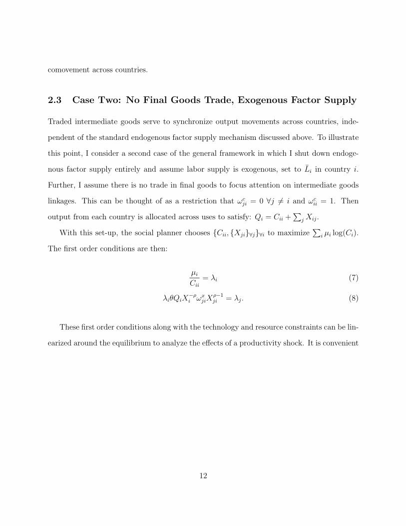
2.3 Case Two: No Final Goods Trade, Exogenous Factor Supply

Traded intermediate goods serve to synchronize output movements across countries, inde-

pendent of the standard endogenous factor supply mechanism discussed above. To illustrate

this point, I consider a second case of the general framework in which I shut down endoge-

nous factor supply entirely and assume labor supply is exogenous, set to Li in country i.

Further, I assume there is no trade in final goods to focus attention on intermediate goods

linkages. This can be thought of as a restriction that ωcji = 0 ∀j 6= i and ωcii = 1. Then

output from each country is allocated across uses to satisfy: Qi = Cii +∑

j Xij.

With this set-up, the social planner chooses {Cii, {Xji}∀j}∀i to maximize∑

i µi log(Ci).

The first order conditions are then:

µiCii

= λi (7)

λiθQiX−ρi ωxjiX

ρ−1ji = λj. (8)

These first order conditions along with the technology and resource constraints can be lin-

earized around the equilibrium to analyze the effects of a productivity shock. It is convenient

12

to stack the equilibrium conditions to generate the following system:

C = −λ (9)

X =1

1− ρ

[Mλλ+MQQ+MQX

](10)

X = W X (11)

Q = SXX + SCC (12)

Q = Z + θX, (13)

where X = [X11, X12, . . . , X1N , X21, X22, . . .]′

is an (N2 × 1) vector and {C, λ, Q, X, Z} are

(N × 1) vectors of the underlying variables for each country. The matrices are defined as

follows:

Mλ ≡ 1N×1 ⊗ IN×N − IN×N ⊗ 1N×1,

MQ ≡ 1N×1 ⊗ IN×N ,

W ≡ [diag(w1), diag(w2), . . .] with wi = [wi1, · · · , wiN ] and wij ≡ωxijX

ρij

Xρj ,

SX ≡

sx1 0 · · ·

0 sx2 · · ·... · · · . . .

with sxi = [sxi1, · · · , wiN ] and sxij =Xij

Qi

,

SC ≡ [diag(sc)] with sci =CiiQi

.

Equations (9)-(13) can be solved to yield a reduced from expression that relates output

in each country to productivity shocks in all other countries via intermediate goods linkages.

Rather than analyze this general case, I turn to an analytically elegant special case.

13

2.3.1 Cobb-Douglas Intermediate Goods Aggregator

To develop intuition regarding how comovement depends on the input sourcing structure,

I assume now that the intermediate goods aggregator takes a Cobb Douglas form. The

production function is then:

Qi = ZiXθi L

1−θi

with Xi =∏j

(Xji)θji/θ ,

(14)

with∑

j θji = θ. With this assumption, equation (10) is replaced by:

X = Mλλ+MQQ. (15)

Using this alternative first order condition, one can show that the proportional change

in output following productivity innovations:

Q = Θ′Q+ Z. (16)

The Θ matrix is a global input-output matrix that summarizes flows of intermediate goods

across countries, with elements θij equal to the share of expenditure on intermediates that

j directly purchases from i as a fraction of the value of output in country j. Rearranging

this equation, I write the change in log output as a reduced form function of productivity

innovations:

Q = [I −Θ′]−1Z. (17)

The matrix [I −Θ′]−1 provides a set of weights that indicate how production in country

i responds to productivity shocks in country j. The weights can be interpreted as the total

14

cost share of intermediates from j in production in country i, taking into account both

direct and indirect purchases of inputs from j. These cost shares reflect global production

sharing relationships. This is intuitive, since a positive productivity shock in country k

benefits countries that use country k goods as inputs. This is true whether they use k goods

directly or whether they rely on country k goods indirectly, in the sense that they source

intermediates from some third country that itself relies heavily on inputs from country k.

This has the implication that output will be correlated for country i and country j when

they have similar overall sourcing patterns.17

2.3.2 Three Country Example

To make these ideas concrete, consider a simple three country version of the Cobb-Douglas

version of the model above in which there are no domestic intermediates (θii = 0). Then the

solution for the vector of output growth takes the form:

Q = [I −Θ′]−1Z with Θ =

0 θ12 θ13

θ21 0 θ23

θ31 θ32 0

. (18)

This solution can be rewritten as:

Q = M

1− θ32θ23 θ21 + θ23θ31 θ31 + θ32θ21

θ12 + θ13θ32 1− θ31θ13 θ32 + θ31θ12

θ13 + θ12θ23 θ23 + θ21θ13 1− θ21θ12

Z, (19)

where M = 1det [I−Θ′ ]−1 . There are two points to note regarding this solution.

17There are two distinct elements to differences in sourcing patterns. First, the overall level of trade willdiffer across countries. Second, conditional on overall openness, bilateral trade patterns also differ.

15

First, for each country, the loadings on foreign country shocks are a function both of

parameters associated with bilateral trade as well as trade with third countries. For ex-

ample, the impact of a productivity innovation in country 2 on country 1’s output is:

M(θ21 + θ23θ31)z2. This effect is a function of both the intensity with which country 1

sources intermediates from country 2 (θ21) and the compound term θ23θ32. This compound

term picks up the indirect effect of country 2 productivity shocks operating via country 1’s

sourcing intermediates from country 3. Specifically, a shock in country 2 raises the supply

of the country 2 intermediate good. This benefits country 1 directly because it uses this

intermediate in production, but also benefits it indirectly because it uses intermediates from

country 3 and country 3 intermediates are in turn produced using country 2 goods. Thus, the

structure of the entire production chain matters, not just bilateral input sourcing patterns.18

Second, there is multiplier effect that controls the magnitude of effect of shocks on each

country. To see this clearly, I re-write output growth for country 1 as:

Q1 = M1

[Z1 +

(θ21 + θ23θ31

1− θ32θ23

)Z2 +

(θ31 + θ32θ21

1− θ32θ23

)Z3

], (20)

where I define M1 = 1−θ32θ23det [I−Θ′ ]−1 to be country 1’s multiplier. M1 summarizes how much

country 1 output increases with shocks to its own productivity and is generally greater than

one. Thus, the sensitivity of output to shocks for different countries can be decomposed into

a country specific effect Mi and a vector of weights on different shocks that varies across

countries.

18In a concrete example, the U.S. benefits from productivity increases in China not only because it importsfrom China, but also because the U.S. sources intermediates from Japan and Japan uses Chinese goods asinputs in production.

16

2.3.3 Gross Output versus Value Added

Thus far, I have implicitly focused the discussion of comovement via intermediate goods

linkages on comovement in gross output. This is because there is an important distinction

between gross output and value added in models with intermediate goods that does not arise

in standard IRBC models without intermediates. To make this distinction explicit, I rewrite

the production function in equation (1) as:

Qi = V 1−θi Xθ

i

with Vi ≡ Z1

1−θi Li.

(21)

The quantity Vi is real value added. Real value added in this framework is a sub-function

of gross output, which itself a composite of productivity and factor inputs (labor). Gross

output then is a composite, homogeneous of degree one, function of real value added and

intermediate goods.19 This set-up implies that real value added can be computed using the

“double-deflation” method, the current best practice in sector-level national accounts. Under

double deflation, nominal output and nominal input purchases for each sector are deflated

via their own price indices. Real value added growth is then equal to: Vi = 1(1−θ)

(Qi − θXi

),

where Qi and Xi are directly measured in the national accounts.20

One important implication of this distinction between real value added and gross output

is that output comoves across countries for two reasons. First, real value added may comove

across countries. Second, input use may comove across countries. In this section with

exogenous factor supply, value added comoves across countries if and only if productivity

19To generalize the definition of real value added, consider a general production function (supressingcountry subscripts and time indexation): Q = f(K,L,X). Then if the production function is weaklyseparable in capital and labor, it can be rewritten as: Q = f(h(K,L), X). The sub-function h(K,L) is then“real value added.”

20Of course, input shares θ are also measured in national accounts.

17

shocks are correlated across countries. On the other hand, gross output can comove across

countries even if productivity shocks are uncorrelated if input use is correlated. Intermediate

goods linkages imply that input use will in fact be correlated, most intensely so for countries

that either have strong bilateral production sharing linkages or are exposed to common

shocks originating in an input supplier to both countries.

With endogenous factor supply, the logic is obviously more complicated, as one layers

this mechanism on top of the standard IRBC transmission of shocks via relative prices and

factor supply. However, distinguishing output and value added comovement in this special

case yields important intuition regarding mechanics that I will exploit below.

3 Dynamic Many Country, Multi-Sector Sector Model

The full model extends the benchmark model in a number of directions. First, the full model

includes both transmission channels discussed above: endogenous factor supply (capital

and labor) and intermediate goods linkages. The model admits both trade in final and

intermediate goods, as well as dynamic adjustment of capital. Second, the full model includes

multiple sectors. Disaggregating the model is important because sectors differ substantially

in both overall openness and integration into cross-border production chains. In specifying

equilibrium in the full model, I need to take a stand on financial market structure. In

what follows, I focus on the case of financial autarky (equivalently, balanced trade) on the

grounds that financial autarky has been shown to generate terms of trade movements and

cross-country correlations that align more closely with data.21

21For example, see Heathcote and Perri (2002) and Kose and Yi (2006). Financial autarky tends to deliverstronger comovement because it shuts down “resource-shifting” effects where in capital is reallocated towardcountries with positive productivity shocks. It is straightforward to consider complete financial markets infuture drafts.

18

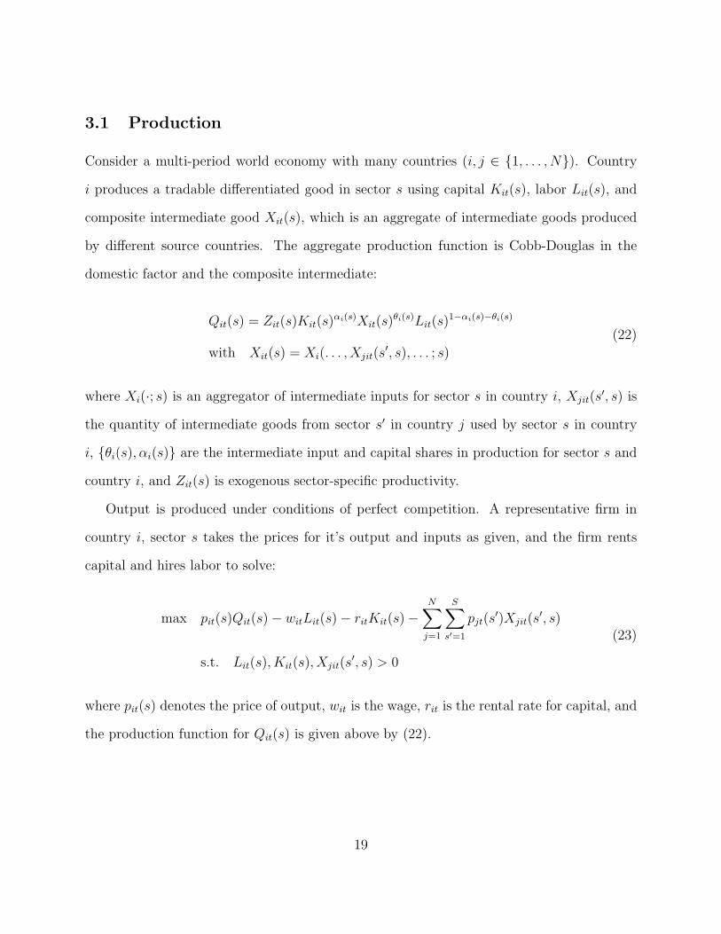
3.1 Production

Consider a multi-period world economy with many countries (i, j ∈ {1, . . . , N}). Country

i produces a tradable differentiated good in sector s using capital Kit(s), labor Lit(s), and

composite intermediate good Xit(s), which is an aggregate of intermediate goods produced

by different source countries. The aggregate production function is Cobb-Douglas in the

domestic factor and the composite intermediate:

Qit(s) = Zit(s)Kit(s)αi(s)Xit(s)

θi(s)Lit(s)1−αi(s)−θi(s)

with Xit(s) = Xi(. . . , Xjit(s′, s), . . . ; s)

(22)

where Xi(·; s) is an aggregator of intermediate inputs for sector s in country i, Xjit(s′, s) is

the quantity of intermediate goods from sector s′ in country j used by sector s in country

i, {θi(s), αi(s)} are the intermediate input and capital shares in production for sector s and

country i, and Zit(s) is exogenous sector-specific productivity.

Output is produced under conditions of perfect competition. A representative firm in

country i, sector s takes the prices for it’s output and inputs as given, and the firm rents

capital and hires labor to solve:

max pit(s)Qit(s)− witLit(s)− ritKit(s)−N∑j=1

S∑s′=1

pjt(s′)Xjit(s

′, s)

s.t. Lit(s), Kit(s), Xjit(s′, s) > 0

(23)

where pit(s) denotes the price of output, wit is the wage, rit is the rental rate for capital, and

the production function for Qit(s) is given above by (22).

19

Labor, capital, and intermediate goods choices for production in country i satisfy:

αi(s)pit(s)Qit(s) = ritKit(s) (24)(θi(s)pit(s)Qit(s)

Xit(s)

)∂Xit(s)

∂Xjit(s′, s)= pjt(s

′) (25)

(1− αi(s)− θi(s))pit(s)Qit(s) = witLit(s). (26)

Output is used as an intermediate good in production and to produce a composite fi-

nal good for consumption and investment. Within each sector, perfectly competitive firms

aggregate final goods from all sources to form a sector-level composite using production

function: Fit(s) = Fi(. . . , Fjit(s), . . . ; s). These sector composites are then aggregated to

form an aggregate final good via a Cobb-Douglas technology: Fit =∏s

Fit(s)γi(s), where

γi(s) is the expenditure share on final goods of type s in country i. Note that I assume that

there is no value added at this stage to be consistent with the accounting conventions in my

input-output data which records the value of retail and distribution services as production

of a separate services sector.

A representative final goods firms maximizes:

max pfitFit −N∑j=1

S∑s=1

pjt(s)Fjit(s), (27)

where pfit is the price of the composite final good and Fit is defined above. Purchases of

individual final goods Fjit for aggregation into the final good satisfy:

(γi(s)p

fitFit

Fit(s)

)∂Fit(s)

∂Fjit(s)= pjt(s). (28)

20

Aggregate final goods are used for consumption and investment: Fit = Cit + Iit.22 Gross

output equals total purchases used as intermediates and to produce final composite goods:

Qit(s) =N∑j=1

S∑s′=1

Fijt(s) +Xijt(s, s′).

3.2 Consumption and Labor Supply

Each country is populated by a representative consumer. The consumer is endowed with

labor (with time endowment normalized to one) that it supplies to firms and consumes final

goods. The representative consumer also owns the capital stock in her country and makes

investment decisions. The capital stock evolves according to: Kit+1 = Iit + (1 − δ)Kit,

where Kit =∑S

s=1Kit(s). Under financial autarky (balanced trade), expenditure on final

goods must equal income in each period for the consumer: pfitFit = witLit + ritKit, where

Lit =∑S

s=1 Lit(s).

The consumer chooses {Cit, Lit, Kit+1} to solve:

max E0

∞∑t=0

βtUi(Cit, Lit)

s.t. pfit(Cit + Iit) = witLit + ritKit

and Kit+1 = Iit + (1− δ)Kit.

(29)

The Euler equation and first-order condition for labor supply are then:

∂Ui(Cit, Lit)

∂Cit= βEt

[∂Ui(Cit, Lit)

∂Cit+1

(rit+1

pfit+1

+ (1− δ)

)](30)

∂Ui(Cit, Lit)

∂Lit=∂Ui(Cit, 1− Lit)

∂Cit

wit

pfit. (31)

22Note that this assumption implies that the aggregator is the same for consumption goods and investmentgoods. This assumption could be relaxed.

21

3.3 Equilibrium

Given a stochastic process for productivity, an equilibrium in the model is a collection of

quantities {Cit, Fit} for each country, {Qit(s), Kit(s), Lit(s), {Fjit(s)}j, {Xjit(s′, s)}j,s′}i,s for

each country-sector, and prices {rit, wit, pfit, {pit(s)}s}i. These must satisfy the producers’

first order conditions (24)-(26) and (28) and the consumer’s Euler equation (30) and first-

order condition for labor supply (31). They must also satisfy market clearing conditions

Qit =∑

j(Fijt + Xijt) and Fit = Cit + Kit+1 − (1 − δ)Kit, the budget constraint pfitFit =

witLit + ritKit, and the production function (22). The equilibrium conditions are collected

explicitly in the appendix [to be completed].

3.4 Calibration

3.4.1 Functional Forms

To calibrate the model, I need to specify functional forms for preferences, the final goods

aggregator, and the intermediate goods aggregator. I assume that preferences are given by:

Ui(Cit, Lit) = log(Cit) − χε1+ε

L(1+ε)/εit . Further, I assume that the final goods are produced

via a CES production function: Fit(s) =(∑

j ωfji(s)Fjit(s)

ρ)1/ρ

, where {ωfji(s)} and ρ are

parameters to be calibrated.

In the benchmark calibration, I assume that the intermediate goods aggregator is Cobb-

Douglas: Xit(s) =∏

j

∏s′ (Xjit(s

′, s))θji(s′,s)/θi(s), where {θji(s′, s)} are parameters be cali-

brated. If the elasticity of substitution between final goods is greater than one, this Cobb-

Douglas assumption implies that the elasticity of substitution within intermediates is lower

than that between final goods. This is consistent with existing work such as Burstein, Kurz,

and Tesar (2008) or Jones (2010), among others, who argue that the scope for substitution

across intermediate goods is lower than for final goods.

22

With these assumptions, I need values for the following parameters: {β, ε} for preferences

and {αi(s), θi(s), {θji(s′, s)}, ρ, {ωfji(s)}, δ} for the technology.23

3.4.2 Technology and Preferences

I set ρ = .33, δ = .1, β = .96, and ε = 1 based on standard values in the literature. I use data

from input-output tables to calibrate the remaining technology and preference parameters.

To calibrate {αi(s), θi(s), {θji(s′, s)}, ρ, {ωfji(s)}, my primary data source is the GTAP

7.1 Data Base assembled by the Global Trade Analysis Project at Purdue University.24 The

data set includes internally consistent bilateral trade statistics combined with domestic and

import input-output tables for 94 countries plus 19 composite regions covering 57 sectors

in 2004. I retain country level data for 22 countries, covering roughly 80% of world GDP,

and aggregate the remaining countries to form a composite “rest-of-the world” region. The

choice of countries is determined primarily by the availability of time series data on gross

production and productivity data (see below).

A key part of the calibration is accurate data on bilateral intermediate and final goods

flows. I construct these data by combining input-output tables with data on bilateral trade,

as in Johnson and Noguera (2010).25 From the GTAP database, I extract disaggregate input

use tables for domestic input purchases and imported inputs. I then use bilateral trade data

to split imported input use across bilateral partners, assuming that input purchases from each

source are proportional to bilateral trade shares within a given sector. I split final goods

23Note, some parameters are not needed to simulate the model. For example, χ governs the level of laborsupplied in the steady state, but model dynamics are independent of this value due to the constant elasticityof labor supply.

24This data is compiled based on three main sources: (1) World Bank and IMF macroeconomic andBalance of Payments statistics; (2) United Nations Commodity Trade Statistics (Comtrade) Database; and(3) input-output tables from national statistical sources. To reconcile data from these different sources,GTAP researchers adjust the input-output tables to be consistent with international data sources.

25Similar approaches have been used by Daudin, Rifflart, and Schweisguth (2009), Koopman, Powers,Wang, and Wei (2010), and Trefler and Zhu (forthcoming).

23

imports across source countries using trade shares in a similar way. This yields bilateral

final and intermediate goods shipments for 57 sectors. I then aggregate data on sectoral

production, trade, final and intermediate shipments across sectors to form two composite

sectors, defined as “goods” (including agriculture, natural resources, and manufacturing)

and “services.”

These data allow me to fit the model to replicate data for output, value added, and

domestic/foreign shipments exactly. I calculate the intermediate goods share of output in

each country and sector θi(s). The median intermediate share for goods producing sectors

is 0.65 for my country sample, while the corresponding share for services is 0.46. Then, I

calculate the capital share in gross output as αi(s) = (1/3)∗ (1− θi(s)), equal to an assumed

capital share in value added (1/3) times the value added to output ratio (1− αi(s)).

The bilateral intermediate and final goods shipments serve as data targets for {θji(s′, s)}

and {ωfji(s)}. According to the producer’s first order condition (25), θji(s′, s) is the ratio of

expenditure on inputs from country j to gross output:

θji(s′, s) =

pj(s′)Xji(s

′, s)

pi(s)Qi(s). (32)

To calibrate {ωfji(s)}, note that the final goods producer’s first order condition (28) can be

rewritten in share form as:

pi(s)Fij(s)

pfjFj= γj(s)ω

fij(s)

(pi(s)

pfj (s)

)−ρ/(1−ρ)

, (33)

wherepi(s)Fij(s)

pfj Fjis the share of final goods of sector s sourced from country i in total final

goods expenditure in j. The share of final expenditure on goods of sector s – γj(s) – can

be computed directly in the data. Then, choosing quantity units so that the price of gross

24

output and the final goods are equal to one in the steady state, {ωfij} can computed by

combining these expenditure shares.

In the data, trade is unbalanced. Therefore, in calibrating the model, I allow steady

state trade to be unbalanced as well to recover ‘true’ preference and technology parameters.

I then solve for dynamics in the model by linearizing around this unbalanced steady state,

assuming that trade imbalances are constant.26 The linearized equilibrium conditions are

included in the appendix [to be completed].

3.4.3 Productivity

To estimate stochastic processes for productivity, I use sectoral productivity data from the

Groningen Growth and Development Centre’s EU KLEMS and 10-Sector databases. Though

ideally one would like estimate the productivity process using data on TFP, data constraints

prevent this for many countries over long periods of time. Therefore, as is standard, I

estimate the productivity process using data on labor productivity.27 Availability of labor

productivity data in the Groningen data limits the number of countries included in the

simulation to 22 countries, covering approximately 80% of world GDP over the period 1970-

2007. I take sectoral labor productivity growth for 19 OECD countries from the EU KLEMS

data, where labor productivity growth is computed as the difference between real value

26An alternative approach would be to calibrate the model to the unbalanced steady state, then solve forand linearize around the corresponding balanced trade equilibrium. In practice, the differences in behaviorof the model linearized around balanced steady state versus imbalanced steady states are small.

27The main data constraint is that estimates of sector level capital stocks and/or labor quality are difficultto obtain. Though motivated by data constraints, using labor productivity in place of TFP implicitlyassumes that capital and/or labor quality dynamics do not drive variation in labor productivity at businesscycle frequencies. This assumption is common in the aggregate IRBC literature: see Backus, Kehoe, andKydland (1992), Heathcote and Perri (2002), or Kose and Yi (2006) for example. Examining countries in theGroningen data for which both TFP and labor productivity growth rates are available for specific periods,the year-on-year growth rates of TFP and labor productivity are roughly proportional, which suggests thisassumption is innocuous.

25

added growth and growth in hours worked for each sector.28 I turn to the 10-Sector data

to compute productivity growth rates for three large emerging markets – Brazil, India, and

Mexico.29 Productivity in this data is measured as the difference between real value added

growth less growth in the number of workers employed.

For each country and sector, I estimate univariate, trend stationary productivity process.

Suppressing constants and time trends, the estimating equation is:

logLP V Ait (s) = λi(s) logLP V A

it−1(s) + εit(s), (34)

where LP V Ait (s) is the level labor productivity (measured using value added) and λi(s) is the

persistence parameter. In a modest departure from the existing literature, I restrict cross-

country spillovers to be equal to zero and further assume that there are no spillovers across

sectors withing a country.30 The correlation of productivity shocks εit(s) is unrestricted.

To compute this correlation, I estimate equation 34 for each country and sector separately,

recover regression residuals εit(s), and then construct the covariance matrix of the shocks as:

Σ ≡ 1T

∑t εtε

′t.

31

To simulate the model, I need to convert the covariance matrix Σ, constructed using

28Countries include Australia, Austria, Belgium, Canada, Denmark, Spain, Finland, France, Germany,Greece, Ireland, Italy, Japan, Korea, Netherlands, Portugal, Sweden, United Kingdom, and the UnitedStates. I omit most Central and Eastern European countries in the data with short time series starting inthe mid-1990s.

29The 10-Sector database includes other smaller emerging markets that could be added to the analysis infuture drafts.

30I restrict cross-country spillovers as a matter of necessity. With N countries and 2 sectors, there aretoo many unrestricted spillover parameters to estimate given the relatively short length of the time seriesavailable. I have experimented with estimation of cross-sector spillovers within countries. Point estimatesfor cross-sector spillovers are generally unstable across countries and imprecisely estimated (often indistin-guishable from zero).

31For three of the forty-four country-sector pairs, the estimated persistence parameters exceed one. Ex-amination of the data indicates that this is due to breaks in the trend for these country-sector time series.For these countries, I estimate productivity processes assuming that each experiences only aggregate pro-ductivity shocks (i.e., productivity growth in goods and services is equal to aggregate productivity growth).These three countries are Italy, India, and Mexico.

26

residuals from estimation of the process for productivity measured using real value added,

into an equivalent covariance matrix for shocks to productivity measured on a gross output

basis. The adjustment multiplies each residual by the ratio of value added to output: ˆεit(s) ≡

(1− θi(s))εit(s).

To understand this adjustment, recall the discussion in Section 2.3.3 about distinguishing

gross output from real value added. At the sector level, gross output is a composite of real

value added and intermediate inputs:

Qit(s) = Vit(s)1−θi(s)Xit(s)

θi(s)

with Vit(s) ≡ Z1

1−θi(s)it Kit(s)

αi(s)

1−θi(s)Lit(s)1−αi(s)−θi(s)

1−θi(s)

(35)

Then, TFP measured using gross output is TFPQ

it(s) = Zit(s), while TFP measured us-

ing real value added is TFPV

it (s) = 11−θi(s)Zit(s). The two TFP measures are related by

TFPQ

it(s) = (1− θi(s))TFPV

it (s), so shocks to productivity measured using value added will

be larger than the corresponding shocks measured using gross output. This explains the need

to adjust Σ and means that the correct covariance matrix for simulation is: Σ = 1T

∑tˆεtˆε′t.

The persistence parameter λi(s) obtained in estimation of 34 can be directly used in simu-

lations, as it does not depend on which definition of productivity is used in the estimation.

In the simulations below, I will use this covariance matrix in two ways. One set of

simulations will allow shocks to be correlated across countries, with correlations determined

by the estimated covariance matrix. This is the standard approach in the literature. The

shortcoming of this approach is that comovement in this set of simulations is driven both by

transmission of shocks across countries via trade linkages and the direct correlation of the

underlying shocks themselves.

To more cleanly identify the trade transmission mechanism, I will also simulate the

27

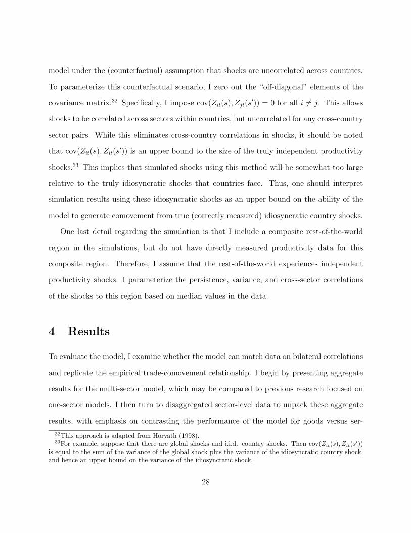
model under the (counterfactual) assumption that shocks are uncorrelated across countries.

To parameterize this counterfactual scenario, I zero out the “off-diagonal” elements of the

covariance matrix.32 Specifically, I impose cov(Zit(s), Zjt(s′)) = 0 for all i 6= j. This allows

shocks to be correlated across sectors within countries, but uncorrelated for any cross-country

sector pairs. While this eliminates cross-country correlations in shocks, it should be noted

that cov(Zit(s), Zit(s′)) is an upper bound to the size of the truly independent productivity

shocks.33 This implies that simulated shocks using this method will be somewhat too large

relative to the truly idiosyncratic shocks that countries face. Thus, one should interpret

simulation results using these idiosyncratic shocks as an upper bound on the ability of the

model to generate comovement from true (correctly measured) idiosyncratic country shocks.

One last detail regarding the simulation is that I include a composite rest-of-the-world

region in the simulations, but do not have directly measured productivity data for this

composite region. Therefore, I assume that the rest-of-the-world experiences independent

productivity shocks. I parameterize the persistence, variance, and cross-sector correlations

of the shocks to this region based on median values in the data.

4 Results

To evaluate the model, I examine whether the model can match data on bilateral correlations

and replicate the empirical trade-comovement relationship. I begin by presenting aggregate

results for the multi-sector model, which may be compared to previous research focused on

one-sector models. I then turn to disaggregated sector-level data to unpack these aggregate

results, with emphasis on contrasting the performance of the model for goods versus ser-

32This approach is adapted from Horvath (1998).33For example, suppose that there are global shocks and i.i.d. country shocks. Then cov(Zit(s), Zit(s′))

is equal to the sum of the variance of the global shock plus the variance of the idiosyncratic country shock,and hence an upper bound on the variance of the idiosyncratic shock.

28

vices sectors and for gross output versus value added. Finally, I use the simulated data to

explore whether augmented trade-comovement regressions with vertical linkages are capable

of identifying the causal influence of input linkages on comovement.

4.1 Aggregate Results

Figure 1 presents bilateral correlations of real value added for each country pair in the model

and data.34 Bilateral correlations are computed as the correlation of year on year growth

rates. Correlations in the model are computed as averages over 500 replications of 35 years

each, roughly the same period over which correlations are computed in the data, using the

estimated covariance of shocks.

As is evident from the figure, model-based correlations are positively related to data-

based correlations, though the fit is far from perfect. The regression line of best fit is

ρij(data) = .26 + .46ρij(model) with standard error on the slope of .07 and R2 = .14. Note

that the model generally under predicts the average correlation in the data, which is quite

reasonable given that there are other shocks outside the model (e.g., demand shocks) driving

correlations in the data that may be on average positively correlated across countries. One

possible candidate for these omitted shocks would be monetary shocks. Indeed, examining

the model’s fit for EU-pairs versus non-EU pairs in Figure 2, the model does a better job

explaining variation in bilateral correlations for non-EU pairs than among EU-pairs.35 While

the model under predicts the average correlation by more and generates a shallower slope

for EU-pairs than non-EU pairs, the slope is significantly positive within both sub-groups.

34I focus on real value added here because I do not have time series data on gross output for all countries.In the model and data, gross output is very highly correlated with real value added at the aggregate level.

35A similar result obtains if I look explicitly at Eurozone pairs versus non-Eurozone pairs. Since severalnon-Eurozone EU countries (e.g., Denmark) peg to the Euro, the EU versus non-EU comparison may bemore appropriate. While the model does not fit EU-pairs in the aggregate, I show below that it does fitEU-pairs well for the goods sector. This is indirect evidence that demand shocks could be an importantdriver of services correlations observed in the data that cannot be explained by the model.

29

To evaluate the trade-comovement puzzle directly in the model, I regress bilateral cor-

relations in the model and data on bilateral trade intensity. Bilateral trade intensity is

measured as: log(EXij+EXjiGDPi+GDPj

), computed for the benchmark 2004 year in my data.36 Table

1 records the regression results for real value added in Panel A and gross output in Panel

B.37 The first column of each panel is based on the data, the second column is based on

the model with correlated shocks, the third column is based on the model with uncorrelated

shocks. Looking at the first column, comovement is clearly positively correlated with log bi-

lateral trade in the data. In the model with correlated shocks, the correlation is significantly

weaker, with the regression coefficients roughly 1/4 to 1/3 of the magnitudes in column one.

Even this, however, perhaps overstates the role of trade per se in generating comovement

in the model. Simulating the model with uncorrelated shocks, the regression coefficients

decline substantially, and become insignificant for real value added. Thus, nearly all of the

positive aggregate correlation in the model with correlated shocks appears to be due to the

correlation of shocks themselves.

4.2 Disaggregate Results

The results above indicate that the aggregate trade comovement puzzle is alive and well,

despite the introduction of intermediate goods into the model. To better understand the

origins of the puzzle and mechanics of the model, I turn to disaggregating the results.

Figure 3 plots bilateral sector-level correlations in the data and model with correlated

shocks for goods and services production separately. The upper panel contains the data

36Because trade shares are stable over time, results are not sensitive as to whether one computes bilateraltrade intensity using trade data single year or averages bilateral trade over time prior to computing themetric. The basic results also hold if the level, rather than log, of bilateral trade intensity is used.

37Gross output correlations are computed using the Groningen EU KLEMS database, which implies thatI cannot calculate correlations for pairs involving Brazil, India, and Mexico. Because I do have real valueadded data for these countries, I do include them in computing real value added correlations. This explainsthe differences in the number of observations across columns for gross output.

30

for each country’s goods sector paired with a bilateral foreign goods sector, and the lower

panel contains the same for services. The results are striking: the model with correlated

shocks does a good job predicting gross output correlations for goods, but fails miserably

for services. The correlation of model and data-based correlations is .47 for goods, and only

.08 for services. Examining Table 2, this basic dichotomy – the model fits relatively well for

goods and poorly for services – is borne out no matter whether one looks at gross output or

real value added, or whether one simulates the model with correlated or uncorrelated shocks

across countries.38 Further, the model even does significantly better for cross-sector pairing

(e.g., mixed services-goods pairs) than for services-services pairs.39

Not surprisingly, the good model fit for goods and poor fit for services manifests it-

self in trade-comovement regressions as well. In these sector level regressions, log bilat-

eral trade intensity between sector s in country i and sector s′ in country j is defined as:

log(EXij(s)+EXji(s

′)GDPi+GDPj

). In Table 3, the coefficient on log bilateral trade intensity in the model

with correlated shocks is roughly 80% the size of the corresponding coefficient in the data for

gross output among goods sector pairs. For services trade, the coefficient in data is nearly

as large as that for goods (and highly significant), but is small and insignificantly different

than zero for services. Even for cross sector pairs, the model-based coefficient is roughly

42%, significantly larger than the aggregate coefficients.

These results refine the trade-comovement puzzle. For the gross output of goods, there

is no puzzle in the model with correlated shocks – the model generates correlations in line

with data. For the gross output of services, the puzzle is severe – the model generates near

zero correlation between bilateral trade and comovement, while there is a strong positive

correlation in the data. Given the large size of the services sector in most OECD countries,

38The model actually generates negative correlations for services out of uncorrelated shocks.39This is likely due to the fact that imported goods are used as an input in the production of services.

31

combining these results means that the aggregate trade-comovement puzzle for gross output

is due in large part to the inability of the model to explain services sector correlations.40

There are two important caveats to this diagnosis of the trade-comovement puzzle. First,

just because the model with correlated shocks replicates bilateral correlations for gross output

does not mean that trade itself is a strong propagator of shocks. Trade may simply be a

proxy for the correlation of shocks, in that countries that trade intensively may have shocks

that are more correlated with one another. Second, the attentive reader will note that I

have thus far focused primarily on the fit of the model for gross output correlations. With

intermediates, real value added and gross output can behave differently in the model. In

fact, quick inspection of Tables 1 or 3 suggest that the model seems to do less well for value

added. I deal with these two issues in turn, focusing on explaining results for goods output in

greater detail. Moreover, to hone in on the propagation mechanism for idiosyncratic shocks,

I focus on results from simulating the model with uncorrelated shocks.

For gross output of goods, propagation of independent shocks explains at most one-third

of the observed comovement in the data. Figure 4 plots actual gross output correlations for

goods against those predicted by the model with uncorrelated shocks. There is a clear positive

relationship, particularly among EU country pairs. The U.S.-Canada outlier is particularly

instructive. The predicted correlation is roughly .23, while the actual correlation in the data

is near .75, roughly a ratio of three to one. More generally, this magnitude is consistent

with the overall spread in the data. Focusing on EU-pairs, predicted correlations vary in the

range (0, .15) while actual correlations lie in the range (.25, .75), so the ratio of the ranges is

roughly .5/.15 or three to one.41

40Further, the model’s inability to generate correlated services output across countries also means that itstruggles to explain aggregate correlations, as in Figure 1.

41In this comparison, I relate changes in comovement across pairs to changes in predicted model correlationsfor EU pairs. This obviously ignores the fact that the model grossly underestimates the median correlation.The median ratio of the model correlation with uncorrelated shocks to the actual correlation is ≈ 10% for

32

These relationships are borne out in looking at the trade-comovement regressions for

goods trade in Panel A of Table 3, where the coefficient generated by the model with un-

correlated shocks is just under 30% the size of the coefficient in the model with correlated

shocks. Thus, while say 2/3 of the goods trade-comovement relationship for gross output is

due to correlated shocks in the model, nearly 1/3 is explained entirely by the propagation

of uncorrelated shocks across countries.

While the model generates comovement in gross output from idiosyncratic shocks, it

generates much weaker comovement in real value added. To see this, I plot the correlation

of gross output against the correlation for real value added for goods sector-pairs in Figure

5. The top two panels are the relationship between these alternative correlations in the

data and in the model with correlated shocks, while the third panel is a depiction of this

relationship in the model with uncorrelated shocks. Whereas correlations for value added

and gross output track each other closely in the upper two panels, there are large differences

between the two in the third panel. Further, the variance of correlations of real value added

is much lower than the variance of correlations in gross output. These discrepancies in the

model with uncorrelated shocks are in and of themselves interesting because they shed light

on the role of intermediate goods in the model.

Recall from the discussion in previous sections that gross output is a composite of real

value added and intermediate inputs, as in Equation (35). The correlation of gross output

can them be decomposed into a weighted sum of the correlation of real value added across

countries, the correlation of input use across countries, and the cross-correlation of real value

added and input use:

ρij(Q) = wvvij ρij(V ) + wxxij ρij(X) + wvxij ρij(V,X) + wxvij ρij(V,X), (36)

EU pairs.

33

where wvvij , wxxij , w

vxij , w

xvij are the appropriate weighting terms for each correlation, themselves

functions of the Cobb-Douglas share parameters and standard deviations of gross output, real

value added, and input use. To provide a visual sense of how these correlations aggregate, I

plot the correlations ρij(V ) and ρij(X) for select country pairs in Figure 6. As is evident, the

correlation in input use across countries dwarfs the correlation in real value added. Further,

the correlation of output lies somewhere in between, near the simple average of these two

correlations.42 Thus, the correlation of gross output is high because intermediate use is

highly correlated, not because value added is highly correlated.

The fact that intermediate use is highly correlated is direct evidence that productivity

shocks are being forcefully transmitted through cross-border production chains in the model.

Because the share of intermediates in gross output for goods is roughly 2/3, this translates

into significant output comovement. On the other hand, value added comovement is not

high, and this drags down overall comovement. Recall that one reason value added comoves

in the model is that factor supply responds to relative prices. The low comovement of real

value added indicates this channel is relatively weak in the model. To raise comovement

in value added, one would need to strengthen this channel. In particular, the model would

need to be adapted to translate the relatively strong comovement in intermediate use into

stronger comovement in value added. I return to this point in the discussion below.

4.3 Vertical Linkages in Trade-Comovement Regressions

Recently, several papers have included proxies for bilateral vertical linkages in trade-comovement

regressions. Di Giovanni and Levchenko (2010) and Ng (2010) both find evidence that ver-

tical linkages at least partly explain why bilateral trade is correlated with comovement. In

42In practice, the weights on each term are approximately equal (roughly 1/4) and the typical cross-correlation (ρij(V,X) or ρij(V,X)) is relatively close to ρij(Q), lying between the extremes of ρij(V ) andρij(X). Hence, the simple average of ρij(V ) and ρij(X) approximates ρij(Q) quite well.

34

previous sections, we have seen that coefficients in trade-comovement regressions can be hard

to interpret because they are likely to be correlated with unobserved shocks. This continues

to be true in trade-comovement regressions with intermediates. It is an open question, then,

whether trade-comovement regressions with vertical linkages can be interpreted as evidence

of a causal relationship between vertical linkages and output comovement?

Because Di Giovanni and Levchenko (2010) examine sectoral data, it is straightforward

to map their empirical exercise to my framework and therefore I focus on their work. Di

Giovanni and Levchenko attack the identification problem by estimating trade-comovement

regressions at the sector level, pooling across sectors, and adding fixed effects to absorb

particular unobservable shocks.43 Specifically, they construct a metric of bilateral vertical

linkages at the sector level to capture the intensity with which exports from sector s in

country i are used as intermediates by sector s′ in country j (and vice versa). This takes

the form:[IO(s, s′)× Exportsij(s) + IO(s′, s)× Exportsji(s

′)], where IO(s, s′) is a measure

of input-output linkages between sectors s and s′ taken from a single country’s input-output

table and Exportsij(s) = log(

EXij(s)

GDPi+GDPj

)is the log of exports from i to j in sector s

normalized by the sum of value added in the source and destination countries.44

Then, Di Giovanni and Levchenko estimate the following regression:

ρij(s, s′) =α + βTradeij(s, s

′)

+ γ[IO(s, s′)× Exportsij(s) + IO(s′, s)× Exportsji(s

′)]

+ FE + εij(s, s′),

(37)

where Tradeij(s, s′) ≡ log

(EXij(s)+EXji(s

′)GDPi+GDPj

)and FE denotes fixed effects that vary by spec-

43Alternative ways to deal with this problem used in the literature include adding additional controls toproxy for possible omitted variables or adopting instrumental variables strategies.

44I use the direct input-requirements IO(s, s′) the U.S. to proxy for cross-sector input links. Di Giovanniand Levchenko also use input links for a single country.

35

ification. One specification includes sector-pair fixed effects, while a second specification

includes sector-pair fixed effects and country-pair fixed effects. These fixed effects are intro-

duced to address concerns about omitted common shocks. The sector pair effects control

for worldwide sector-specific shocks (possibly correlated across sectors) that hit all countries

simultaneously. The country pair fixed effects control for aggregate shocks that may be

correlated across countries, but hit all sectors symmetrically within each country.45

I report the results of running these regressions in my data in Table 4. Focusing on

results for gross output, the regression results in the actual data are generally consistent

with those reported in Di-Giovanni Levchenko. Both bilateral trade and vertical linkages

(Trade× IO) are positively correlated with bilateral sector-level comovement.46 Examining

results in the model with correlated shocks, vertical linkages remain significant and the

coefficient magnitudes are the same or larger than those found in the data. Turning to the

model with uncorrelated shocks, however, the magnitude of the coefficient on vertical linkages

drops significantly, explaining only perhaps 17− 33% of the magnitude of the coefficients in

the data.47 Recall that the fixed effects are intended to control for correlated shocks driving

correlations in the data. If these fixed effects adequately control for these shocks, one should

expect that regression results in the model with uncorrelated shocks to be similar to those

in the data (alternatively, the model with correlated shocks). Given that they are not, this

suggests that vertical linkages proxies in the data may themselves be picking up shocks that

vary by country-pair and sector-pair that the fixed effects cannot absorb.

45Ng (2010) embeds a vertical linkages metric into an aggregate trade-comovement regression, and thereforecannot use pair fixed effects to absorb common shocks. Instead, he includes other possible determinants ofcorrelations (e.g., financial openness, output composition, etc.) directly as control variables in the regression.

46Though trade intensity is not significant when country fixed are included, vertical linkages are significantwith both sets of fixed effects. One point to note is that my country sample is much smaller than Di Giovanniand Levchenko (2010), so lower significance levels may be expected.

47Note that looking at real value added, the model with correlated shocks continues to generate coefficientson vertical linkages similar to those in the data, though smaller in magnitude. However, the sign on verticallinkages actually flips sign in regressions in the simulated data with uncorrelated shocks.

36

In evaluating these results, one might be concerned that this coefficient in stability across

the model and data might be related to the fact that the vertical linkages metrics used are

not theoretically motivated. Therefore, let me make the same basic point using a convenient

proxy for the role of vertical linkages in generating output comovement suggested by the

model.

If we define Θ = [I − Θ′]−1, then equation (17) implies that the covariance of output

growth in countries i and j is:

cov(Qi, Qj) = Θ(i, :) ΣZ Θ(j, :)′, (38)

where ΣZ is the covariance matrix for productivity innovations Z, and Θ(k, :) is the kth row

of Θ. When productivity innovations are independent across countries with variance σ2k for

country k, then:

cov(Qi, Qj) =∑k

Θ(i, k)σ2kΘ(j, k). (39)

This covariance is increasing in the similarity between the weighting vectors for country i and

country j. And these vectors of shock loadings are themselves functions of the input-output

structure. Countries with more similar input sourcing and production sharing patterns will

tend to have more similar exposure to shocks.

While the Cobb-Douglas, exogenous factor supply version of the model suggests that [I−

Θ′]−1 provides the correct sourcing weights, the general model generates more complicated

weighting formulas, where input sourcing patterns are one key component among a variety

of forces. Therefore, rather than relying too heavily on the sourcing weights from the Cobb-

Douglas case, I focus on a simple and general metric for input sourcing similarity, based

loosely on work by Conley and Dupor (2003).48 I characterize each destination country

48Conley and Dupor (2003) model correlation across sectors within the domestic economy as a function

37

by an 2N-dimensional vector of cost shares on inputs from each source country. For each

country pair, I compute a sourcing similarity index: SSij = 1 − ‖Θ(:, i)−Θ(:, j)‖, where

‖ · ‖ is a Euclidean distance operator and high values of SSij indicate similar input sourcing

patterns.49 The basic prediction is that output comovement should be positively correlated

with input sourcing similarity SSij.

Table 5 presents estimates from trade-comovement regressions controlling for sourcing

similarity in the data and model for goods production.50 In the data and model with cor-

related shocks, both trade and sourcing similarity are positively correlated with bilateral

comovement, with roughly similar magnitudes in both cases. In contrast, the correlation of

sourcing similarity and bilateral trade with comovement is much weaker in the model with

uncorrelated shocks. While still significant, the partial correlation is only 11% the size of

the correlation in the data. As in the previous regressions, a natural interpretation of this is

that sourcing similarity is correlated with output comovement in the data primarily because

it is correlated with omitted shocks.

5 Complementarity and Comovement

A recent strain of thought holds that disruptions in input-sourcing produce large output

losses because inputs are complements in production.51 There are several different formu-

lations of this basic idea. First, inputs may complements to each other. In this instance,

of the similarity between sectors in terms of their input use, measured using input cost shares.49In practice, this sourcing similarity metric is highly correlated with an alternative metric that takes the

Euclidean distance between rows of the [I −Θ′]−1 matrix.50In the data-based regression, I exclude bilateral pairs involving Italy. Including the Italian data weakens

the correlations in the data, as Italy in the data appears too have too high correlations in output with othercountries given it’s level of input sourcing similarlity. This is mostly due to Italy’s agriculture and naturalresources sector. If one looks at manufacturing correlations and sourcing similarity only (rather than allgoods) Italy does not appear unusual.

51For example, see Burstein, Kurz, and Tesar (2008), Jones (2010), or the discussion in Di Giovanni andLevchenko (2010).

38

complementaries among inputs could be symmetric, or complementaries could vary among

subsets of inputs (e.g., home and foreign inputs could be complements, while foreign inputs

are substitutable among themselves). Second, inputs may be complementary to other factors

of production. Put differently, inputs may be complementary to value added.

While the predominant view seems to be that the first type of complementarity is the

most important, the results above seem to suggest that the second could play a large role.

Specifically, the model generates substantial comovement in intermediate goods use, but

it fails to translate this into comovement in value added. One way to induce additional

comovement in value added is to assume that intermediates are complements to value added.

This then motivates a quantitative exploration of the role of this form of complementarity

in amplifying comovement in the model.

[To Be Completed.]

6 Conclusion

This paper uses a multi-sector, many country extension of the IRBC model with trade

in both final and intermediate goods to dissect the trade-comovement puzzle. Using the

model, I attempt to refine our understanding of the trade comovement puzzle along several

dimensions.

First, input trade does not resolve the aggregate trade-comovement puzzle in a straight-

forward manner. That said, input trade does appear to play a role in explaining the relatively

good fit of the model for the gross output of goods. Surprisingly, however, transmission of

shocks through intermediate input channels does not appear to generate strong comovement

in value added. This points the way toward adaptations of the standard framework, specifi-

cally introducing greater complementarity between real value added and input use, that may

39

amplify the strength of this transmission channel.

Second, and more generally, the aggregate trade comovement puzzle is linked to the

model’s inability to generate a positive correlation between bilateral trade and comovement

in services output across countries. This suggests that closing the gap between theory and

data will require expanding the set of shocks considered beyond productivity to include

shocks that synchronize services more forcefully. This is perhaps not as easy as it sounds,

given that demand shocks tend to be concentrated on demand for goods, specifically durable

goods.

Third, trade-comovement regressions are difficult to interpret because it is not generally

possible to control unobservable common shocks. This is true for plain-vanilla specifications,

as well as augmented specifications that include proxies for vertical linkages and/or employ

sector-level data with fixed effects. Model simulations with uncorrelated shocks suggest that

the “causal” role of bilateral trade and/or vertical linkages is much smaller than suggested

by raw regression estimates.

40

References

Ambler, S., E. Cardia, and C. Zimmerman (2002): “International transmission of thebusiness cycle in a multi-sector model,” European Economic Review, 46, 273–300.

Arkolakis, C., and A. Ramanarayanan (2009): “Vertical Specialization and Inter-national Business Cycle Synchronization,” Scandinavian Journal of Economics, 111(4),655–680.

Backus, D., P. Kehoe, and F. Kydland (1994): “Dynamics of the Trade Balance andthe Terms of Trade: The J-Curve?,” The American Economic Review, 84(1), 84–103.

Baxter, M. (1995): “International Trade and Business Cycles,” in Handbook of Interna-tional Economics, ed. by G. Grossman, and K. Rogoff, vol. 3, chap. 35, pp. 1801–1864.Elsevier.

Baxter, M., and M. Kouparitsas (2005): “Determinants of business cycle comovement:a robust analysis,” Journal of Monetary Economics, 52, 113–157.

Bems, R., R. Johnson, and K.-M. Yi (forthcoming): “Demand Spillovers and the Col-lapse of Trade in the Global Recession,” IMF Economic Review, 58(2).

Bergin, P., R. Feenstra, and G. Hanson (2009): “Offshoring and Volatility: Evidencefrom Mexico’s Maquiladora Industry,” The American Economic Review, 99(4), 4.

Burstein, A., C. Kurz, and L. Tesar (2008): “Trade, production sharing, and theinternational transmission of business cycles,” Journal of Monetary Economics, 55, 775–795.

Calderon, C., A. Chong, and E. Stein (2007): “Trade intensity and business cyclesychronization: Are developing countries any different?,” Journal of International Eco-nomics, 71, 2–21.

Carvalho, V. M. (2008): “Aggregate Fluctuations and the Network Structure of Intersec-toral Trade,” Unpublished, CREi and Universitat Pompeu Fabra.

Cole, H., and M. Obstfeld (1991): “Commodity trade and international risk sharing,”Journal of Monetary Economics, 28, 3–24.

Conley, T., and B. Dupor (2003): “A Spatial Analysis of Sectoral Complementarity,”Journal of Political Economy, 111, 311–352.

Daudin, G., C. Rifflart, and D. Schweisguth (2009): “Value-Added Trade andRegionalization,” Unpublished Manuscript, OFCE de Sciences Po.

41

di Giovanni, J., and A. Levchenko (2010): “Putting the Parts Together: Trade, Verti-cal Linkages and Business Cycle Comovement,” American Economic Journal: Macroeco-nomics, 2(2), 95–124.

Drozad, L., and J. Nosal (2008): “Long-Run Price Elasticity of Trade and the Trade-Comovement Puzzle,” Unpublished, University of Wisconsin.

Dupor, B. (1999): “Aggregation and irrelevaqnce in multi-sector models,” Journal of Mon-etary Economics, 43, 391–409.

Engel, C., and J. Wang (2009): “International Trade in Durable Goods: UnderstandingVolatility, Cyclicality, and Elasticities,” Unpublished Manuscript, University of Wisconsin.

Foerster, A., P.-D. Sarte, and M. Watson (2008): “Sectoral vs. Aggregate Shocks: AStructural Factor Analysis of Industrial Production,” Unpublished Manuscript, PrincetonUniversity.

Frankel, J., and A. Rose (1998): “The Endogeneity of the Optimum Currency AreaCriteria,” The Economic Journal, 108, 1009–1025.

Heathcote, J., and F. Perri (2002): “Financial autarky and international businesscycles,” Journal of Monetary Economics, 49, 601–627.

Horvath, M. (1998): “Cyclicality and Sectoral Linkages: Aggregate Fluctuations fromIndependent Sectoral Shocks,” Review of Economic Dynamics, 1, 781–808.

(2000): “Sectoral shocks and aggregate fluctuations,” Journal of Monetary Eco-nomics, 45, 69–106.

Imbs, J. (2004): “Trade, Finance, Specialization, and Synchronization,” The Review ofEconomics and Statistics, 86, 723–734.

Inklaar, R., R. Jong-A-Pin, and J. de Haan (2008): “Trade and business cycle syn-chronization in OECD countries – A re-examination,” European Economic Review, 52(4),646–666.

Johnson, R., and G. Noguera (2010): “Accounting for Intermediates: Production Shar-ing and Trade in Value Added,” Unpublished Manuscript, Dartmouth College.

Jones, C. (forthcoming): “Intermediate Goods and Weak Links in the Theory of EconomicDevelopment,” American Economic Journal: Macroeconomics.

Koopman, R., W. Powers, Z. Wang, and S.-J. Wei (2010): “Give Credit Where CreditIs Due: Tracing Value Added in Global Production Chains,” NBER Working Paper 16426.

42

Kose, M. A., and K. M. Yi (2006): “Can the standard international business cyclemodel explain the relation between trade and comovement?,” Journal of InternationalEconomics, 68, 267–295.

Long, J., and C. Plosser (1983): “Real Business Cycles,” Journal of Political Economy,91(1), 39–69.

Ng, E. C. (2010): “Production fragmentation and business-cycle comovement,” Journal ofInternational Economics, 82(1), 1–14.

O’Mahoney, M., and M. Timmer (2009): “Output, Input and Productivity Measures atthe Industry Level: The EU KLEMS Database,” The Economic Journal, 119, F374–F403.

Shea, J. (2002): “Complementarities and Comovements,” Journal of Money, Credit, andBanking, 34, 412–433.

Trefler, D., and S. C. Zhu (forthcoming): “The Structure of Factor Content Predic-tions,” Journal of International Economics.

Yi, K.-M. (2003): “Can Vertical Specialization Explain the Growth of World Trade?,”Journal of Political Economy, 111, 52–102.

43

Table 1: Aggregate Trade-Comovement Regressions: Data and Model

Panel A: Real Value Added

Data Model (corr. shocks) Model (uncorr. shocks)

Log Bilateral Trade 0.104*** 0.025* 0.001(0.014) (0.013) (0.000)

N 231 231 231R-sq 0.18 0.02 0.01

Panel B: Gross Output

Data Model (corr. shocks) Model (uncorr. shocks)

Log Bilateral Trade 0.093*** 0.035*** 0.008***(0.012) (0.013) (0.001)

N 171 231 231R-sq 0.25 0.03 0.36

Robust standard errors in parentheses. Significance levels: * p < .1 , ** p < .05,*** p < .01. Constants included in all regressions.

44

Table 2: Correlation of Model Predicted vs. Actual Correlations, by Sector Pair

Panel A: Gross Output – Model with Correlated Shocks

Sector Pair Correlation N

Goods 0.47 171Services 0.08 171Cross 0.21 342

Panel B: Gross Output – Model with Uncorrelated Shocks

Sector Pair Correlation N

Goods 0.52 171Services -0.22 171Cross 0.30 342

Panel C: Real Value Added – Model with Correlated Shocks

Sector Pair Correlation N

Goods 0.51 231Services 0.25 231Cross 0.42 462

Panel D: Real Value Added – Model with Uncorrelated Shocks

Goods 0.25 231Services -0.11 231Cross 0.14 462

45

Table 3: Trade-Comovement Regressions, by Sector Pair

Panel A: Gross Output

Data Model (correlated shocks) Model (uncorrelated shocks)Goods Services Cross Goods Services Cross Goods Services Cross

Log Bilateral Trade 0.090*** 0.071*** 0.071*** 0.072*** 0.009 0.030*** 0.020*** -0.002*** 0.010***(0.013) (0.013) (0.009) (0.012) (0.012) (0.008) (0.001) (0.001) (0.001)

N 171 171 342 231 231 462 231 231 462R-sq 0.23 0.15 0.16 0.13 0.00 0.03 0.56 0.03 0.33

Panel B: Real Value Added

Data Model (correlated shocks) Model (uncorrelated shocks)Goods Services Cross Goods Services Cross Goods Services Cross

Log Bilateral Trade 0.098*** 0.054*** 0.055*** 0.055*** 0.006 0.019** 0.003*** -0.003*** 0.005***(0.012) (0.013) (0.009) (0.012) (0.012) (0.008) (0.001) (0.001) (0.000)

N 231 231 462 231 231 462 231 231 462R-sq 0.22 0.07 0.08 0.09 0.00 0.01 0.10 0.09 0.17

Robust standard errors in parentheses. Significance levels: * p < .1 , ** p < .05, *** p < .01. Constantsincluded in all regressions.

46

Table 4: Disaggregate Trade-Comovement Regressions with “Vertical Linkages”

Panel A: Gross Output

Sector-Pair Fixed Effects Sector-Pair & Country-Pair Fixed EffectsData Model Model Data Model Model

(corr. shocks) (uncorr. shocks) (corr. shocks) (uncorr. shocks)

Log Bilateral Trade 0.046*** 0.007 0.005** 0.025 0.004 0.007***(0.013) (0.013) (0.002) (0.017) (0.015) (0.002)

Trade x IO 0.059** 0.056** 0.010*** 0.036** 0.061*** 0.012***(0.024) (0.024) (0.004) (0.018) (0.018) (0.003)

N 684 924 924 684 924 924R-sq 0.23 0.08 0.44 0.68 0.65 0.64

Panel B: Real Value Added

Sector-Pair Fixed Effects Sector-Pair & Country-Pair Fixed EffectsData Model Model Data Model Model

(corr. shocks) (uncorr. shocks) (corr. shocks) (uncorr. shocks)

Log Bilateral Trade 0.021 0.001 0.005*** -0.031** 0.003 0.008***(0.014) (0.013) (0.001) (0.013) (0.018) (0.002)

Trade x IO 0.088*** 0.048** -0.006*** 0.075*** 0.054*** -0.005***(0.024) (0.024) (0.002) (0.016) (0.021) (0.002)

N 924 924 924 924 924 924R-sq 0.13 0.05 0.15 0.70 0.47 0.36

Robust standard errors in parentheses. Significance levels: * p < .1 , ** p < .05, *** p < .01. Constantsincluded in all regressions.

47

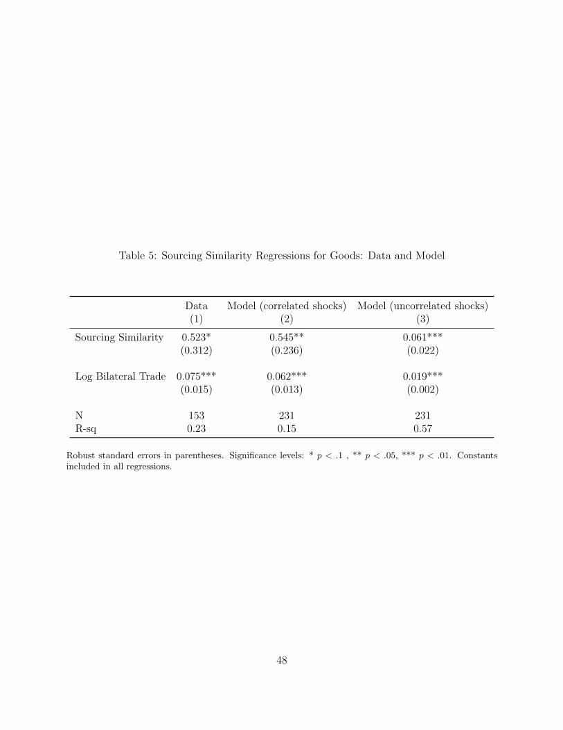
Table 5: Sourcing Similarity Regressions for Goods: Data and Model

Data Model (correlated shocks) Model (uncorrelated shocks)(1) (2) (3)

Sourcing Similarity 0.523* 0.545** 0.061***(0.312) (0.236) (0.022)

Log Bilateral Trade 0.075*** 0.062*** 0.019***(0.015) (0.013) (0.002)

N 153 231 231R-sq 0.23 0.15 0.57

Robust standard errors in parentheses. Significance levels: * p < .1 , ** p < .05, *** p < .01. Constantsincluded in all regressions.

48

Figure 1: Aggregate GDP: Data vs. Model with Correlated TFP Shocks

Figure 2: Aggregate GDP: Data vs. Model with Correlated TFP Shocks

49

Figure 3: Correlations in Data vs. Correlations in Model with Correlated Shocks

50

Figure 4: Correlations in Data vs. Correlations in Model with Uncorrelated Shocks

51

Figure 5: Correlations in Gross Output vs. Correlations in Value Added: Model and Data

52

Figure 6: Correlations of Goods Output and Components in Model with Uncorrelated Shocks

53