International Comovement of Equity Markets and

Foreign Exchage

Markus Hochstottera,1, Paul Weskamp2

aSchool of Economics and Business Engineering, Karlsruhe Institute of Technology,Germany

Abstract

With this article, we contribute to the analysis of comovement of equity mar-kets and foreign exchange rates using a large international data set coveringthe most important markets. We measure the mutual influence on the levelsby correlation, linear regression, vector autoregression, and Granger causal-ity as well as the dynamic in the comovement behavior by means of DCC-GARCH. We find significant negative as well as positive comovement. More-over, we observe that comovement measured by linear dependence tends tobe much more stable in developing economies than in the leading economies.On the other hand, we generally do not find significant regional clusters ofcomovement behavior.

Key words:

Email addresses: markus.hoechstoetter@kit.edu (Markus Hochstotter)1Markus Hochstotter is an assistent professor at the Chair of Statistics, Economet-

rics and Mathematical Finance at the School of Economics and Business Engineering,Karlsruhe Institute of Technology, Germany.

2Paul Weskamp is a master student at the Chair of Statistics, Econometrics and Mathe-matical Finance at the School of Economics and Business Engineering, Karlsruhe Instituteof Technology, Germany.

April 23, 2012

1. Introduction

In increasingly globally active financial markets, the aspect of comove-

ment between currencies and international portfolio holdings becomes an

issue of paramount importance (Johnson and Soenen, 2009). Negligance

of which might easily counteract portfolio management objectives. Conse-

quently, in a world of global equity investments, exchange rates are just as

relevant for portfolio returns as the equity returns themselves. Moreover,

the foreign exchange market actually represents the largest asset class in the

world.3 It is the aim of this work to contribute with a thorough econometric

analysis of comovement between equity markets and foreign exchange, whose

results can immediately benefit the investor.

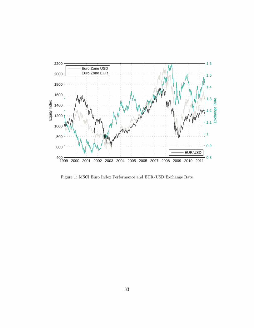
Visual examination of equity market and exchange rate plots reveals many

similarities. All markets and exchange rates are affected to some extent by

global developments. As an example, we present the development of the euro

zone in Figure 1. In the first years of examination, the dot-com bubble, the

subsequent crash, and recovery therefrom dominate the picture. The follow-

ing years are mostly characterized by equity market growth, which peaks with

the United States real estate bubble. The collapse of the bubble is then suc-

ceeded by recovery and turbulent times afterwards. A certain Comovement

is visually detectable to some extent. However, comovement characteristics

differ greatly between different markets. Moreover, comovement is more ev-

ident in some periods than in others.

In his seminal work on portfolio theory, Markowitz (1952) suggests that

3See, for example, Galati and Melvin (2004).

2

minimization of risk can be achieved through diversification. In an extension

of the original idea, Sharpe (1964) considers the presence of undiversifiable,

systematic risk in his popular capital asset pricing model. Asset excess re-

turns depend to some extent on the market excess returns linearly. That is,

he considers comovement between assets and some market where comove-

ment is expressed as correlation. More generally, Ross (1976) introduces the

sensitivity of asset prices to n economic factors. Consequently, the arbitrage

pricing theory acknowledges price comovements with further factors.

Comovement in terms of asset price dependencies is a common and well-

studied phenomenon. Common economic factors, which influence expected

discounted returns, serve as primary explanation. However, plenty of research

suggests that there is asset price comovement in excess of what any economic

explanatory factors could account for. Campbell et al. (2001) notice that,

even though comovement in the United States had decreased somewhat dur-

ing the decades prior to their study, it is still beyond that measurable by

the covariance. This excess comovement is commonly explained by investor

sentiment and irrational “herd behavior”.

The most intuitive measures of comovement are based on correlation.

Nevertheless, defining comovement is not trivial. There is plenty of research

about comovement but no common understanding of the term. Baur (2003)

notes that there is no clear and unambiguous definition of comovement and

no unique measure associated with it. Campbell et al. (2001) define it as

the part of stock price variation that cannot be explained by market or

industry movements. It is not clear from the start which methodology suits

the purpose best. Hence, in our analysis of comovement between stocks and

3

foreign exchange prices, we will use several different measures.

To introduce the reader to the matter as well as present the state of re-

search, we provide section 2. Each model used in our study will be presented

in detail. The data consisting of 30 equity indices and 30 exchange rates

series will be introduced in chapter 4. Section 5 will present the results. To

conclude, section 6 will summarize.

4

2. Literature

The academic literature related to the term comovement is manifold.

However, to the best of our knowledge, the term appears in an economic

context, only, and mostly in the field of finance where it is used to describe

the coherence between financial asset prices or asset returns. The bulk of the

comovement literature in this context concentrates on equity with particular

focus on international markets, fundamentals, individual stocks, or stocks

and other securities.

By far, most research focuses on comovement of equity prices or returns.

In particular, comovement of international equity markets on a regional or

global scale is thoroughly studied.

Being among the first to go into this direction, Agmon (1972) finds sup-

port for the hypothesis that share price comovement in the United States,

United Kingdom, Germany, and Japan behave as if there were only one com-

mon capital market. Panton et al. (1976) find different degrees of similarity

of return comovement between twelve major international equity markets.

Evidence that comovement is not simply equivalent to fundamentals is pro-

vided, for example, by Shiller (1989) who reports evidence of stock price

comovement between the United States and United Kingdom stock prices in

excess of what dividend comovement would suggest.

It is commonly observed that comovement changes in time. Using a com-

mon factor model, Morana and Beltratti (2008) document that volatility

comovement between the US, UK, German, and Japanese markets, respec-

tively, have become more pronounced, in the period 1973–2004. Bollerslev

(1990) documents rising comovement between five nominal European U.S.

5

dollar exchange rates following the inception of the European Monetary Sys-

tem. To do so, he uses the constant correlation multivariate GARCH model.

They find volatility components strongly correlated between the currencies.

Moreover, they find a much higher likelihood for their model than for the

CC-GARCH model. Though not focussing on volatility comovement, John-

son and Soenen (2009) suggest that a higher share of imports by Germany

from other EU countries as well as fluctuations and increased volatility in

the exchange rate have negative effects on stock market comovement.

There is research that suggests that comovement increases during periods

of turmoil at the financial markets. Especially the black Monday in 1987, the

1994 Mexican peso crisis, the Asian financial crisis of 1997, and the collapse

of the dot-com bubble in 2000 are well examined considering changes of asset

price comovements. Wen-Chung and Hsiu-Ting (2008) suggest that comove-

ment between stocks in high-tech industries is stronger than in traditional

industries and stronger in bull than in bear markets. This is a well known

fact. Building on Veldkamp (2006) and Brockman et al. (2010), Hochstotter

et al. (2010) analyze the impact of news on stock return comovement. Defin-

ing a measure of news comovement, they find that stock return comovement

is to some extent driven by the degree of commonality in firm specific news.

Lee and Kim (1993) document a strengthening of comovement after the

1987 stock market crash. Brooks and Del Negro (2004) applying analysis

of variance and mean absolute deviations of coefficients in a cross-sectional

regression model cannot reject the hypothesis that the rise in comovement

during the period between 1985 and 2002 was only temporary due to the

stock market IT bubble. As explanation of rising comovement, Connolly

6

et al. (2007) regarding United States and European equity markets find that

comovement is stronger in uncertain time periods. This is in agreement with

the view presented Hochstotter et al. (2010) and Brockman et al. (2010), for

example.

Research on comovement between stock returns and economic fundamen-

tal values such as inflation, interest rate, etc. is also very common. For exam-

ple, Karolyi and Stulz (1996) do not find evidence that US macroeconomic

announcements, foreign exchange shocks, and treasury bill returns have in-

fluence on return correlations between US and Japanese market returns.

There has also been research on comovement of stock returns and bond

yields and, to a lesser extent, on comovement between equity returns and

returns of different kinds of securities, such as asset backed securities or

among bond yields. For example, Shiller and Beltratti (1992) document

negative correlation between stock prices and bond yields in the US and the

UK between 1871 and 1989. Jobst (2006) examine comovement between

asset-backed securities and stocks using a vector autoregressive model.

Using regression analysis, Ammer et al. (2011) study the comovement

between emerging market and non-emerging market stock and bond markets

in the period 1992–2009. Their study suggests that longer period emerging

market bond and stock prices have on average moved in the same direction

as the prices of non-emerging market risky assets. However, they also find

evidence that the responsiveness of emerging market asset prices to move-

ments in U.S. high-yield corporate bond spreads has declined over the past

decade.

We conclude this section with the literature mostclosely related to ours.

7

Granger et al. (2000) point out the contrasting theories of the “traditional”

approach, i.e. currencies lead stocks, and the “portfolio” approach, i.e. stocks

lead currencies negatively correlated. Using daily Asian data between 1986

and 1998, support of the traditional approach is found in South Korea while

the portfolio approach is supported in Hong Kong. In the other Asian mar-

kets, the relationships are bidirectional. Based on monthly Swedish data in

the period 1993-98, Hatemi-J and Irandoust (2002) prove that stocks uni-

directionally Granger cause exchange rates. With the aid of a friction and

Tobin model, Hashimoto and Ito (2004) analyze Asian stocks and curren-

cies in the period 1997-99. They find that the Hong Kong stock market

was significantly affected by the Indonesian, Korean, and Thai currency de-

preciations. Dimitrova (2005) focussing on the US and UK 1990 and 2004

finds weak evidence of currency depreciation caused by an upward trend in

the stock market. Aydemir and Demirhan (2009) using data from Turkey

between 2001 and 2008 find evidence of a bidirectional causal relationship

between exchange rates and stock prices.

8

3. Methodology

3.1. Covariance, Correlation, and Linear Regression

Since covariance, Pearson correlation, and the concept of linear regression

are well-known, we simply state a few details. For series of length T , we use

the unbiased covariance estimate with standard error

σCov = Cov(x, y) ·√

2

T − 1

as established by Ahn and Fessler (2003). For the assessment of the goodness-

of-fit of the regression, in addition to the R2, we also use the adjusted coef-

ficient of determination

R2 = 1− (1−R2)T − 1

T − p− 1

where p is the total number of regressors in the linear model excluding the

constant term.

3.2. Vector Autoregression and Granger Causality

To test whether one can predict equity market movements by foreign ex-

change movements or the converse, the time series are tested for Granger

causality. According to Granger (1969), x causes y if x contains informa-

tion that helps predict y above and beyond the information contained in

past values of y alone. This technique can be found often in the context

of comovement as, for example, by Jang and Sul (2002) or D’Ecclesia et al.

(2006).

9

Granger causality is analyzed in a vector autoregression model of the form y1t

y2t

=

A11(L) A11(L)

A21(L) A22(L)

y1t

y2t

+

c1

c2

+

ε1

ε2

The yit, i = 1, 2 denote the endogenous variables, ci denote constants, and

εi denote independent disturbances at time t. The model parameters Aij(L)

take the form∑l

k=1 aijkLk, where L is the lag operator defined by Lkyt =

yt−k, and l is the lag length.

The choice of lag length can be crucial. Thornton and Batten (1984) show

that Granger causality tests can come to converse results, if conducted with

different lag lengths. For an objective selection of lag length, the Bayesian

Information Criterion (BIC) of Schwarz (1978)

BIC = log σ2ε +

1 + 2l +m

T∗ log T .

is employed where m is the number of exogenous instantaneous variables.

To test for Granger causality based on T observations, the sum of squared

residuals of the models (including contemporaneous as well as l lagged ob-

servations) before and after inclusion of the corresponding causal series are

compared applying the F -statistic

F =RSS1−RSS2

lRSS2

T−(1+2l+m)

where RSS1 and RSS2 denote the residual sums of squares with and without

consideration of xt, respectively.

10

3.3. Geweke’s Measure for Linear Dependence

Geweke (1982) proposes additional linear measures, which are occasion-

ally employed with respect to comovement analysis, predominantly for the

detection of the influence of fundamentals on comovement. It is assumed

that for the two time series xt and yt, there are autoregressive representa-

tions, such that:

xt =∞∑s=1

e1sxt−s + u1t, Σ1 = V ar(u1t)

yt =∞∑s=1

g1sxt−s + v1t, T1 = V ar(v1t)

and vector autoregressive representations of the form

xt =∞∑s=1

e2sxt−s +∞∑s=1

f2syt−s + u2t, Σ2 = V ar(u2t)

yt =∞∑s=1

g2sxt−s +∞∑s=1

h2syt−s + v2t, T2 = V ar(v2t).

According to Geweke’s work, linear feedback from y to x is measured as

follows:

Fy→x = ln (|Σ1| / |Σ2|) (1)

and linear feedback from x to y symmetrically:

Fx→y = ln (|T1| / |T2|) . (2)

11

The residual vectors u2t and v2t are both serially uncorrelated, but can be

correlated with each other contemporaneously. The covariance matrix Υ of

the vector autoregression residual series therefore is

Υ = V ar

u2t

v2t

=

Σ2 C

C ′ T2

.

This leads to Geweke’s measure of instantaneous feedback

Fx·y = ln (|T2| · |Σ2| / |Υ|) . (3)

Geweke proposes the following measure for linear dependence

Fx,y = ln (|Σ1| · |T1| / |Υ|)Fx,y = Fy→x + Fx→y + Fx·y.

as the sum of the three types of linear feedback (1), (2), and (3) established

above.

Hence, the measure considers (instantaneous) linear regression and vector

autoregression aspects. Geweke was the first one to point out the decompo-

sition such that linear dependence is the sum of linear feedback from x to y,

linear feedback from y to x, and mutual instantaneous linear feedback.

3.4. Dynamic Conditional Correlation GARCH (DCC-GARCH)

It is well known that financial time series tend to feature heteroscedas-

ticity. However, the dependence structure between equity markets and for-

eign exchange is dynamic. Based on the initial autoregressive conditional

heteroscedasticity models by Engle (1982) and Bollerslev (1986), the multi-

12

variate dynamic conditional correlation (DCC-GARCH) model can feature

both, conditional (co-)variances and conditional correlations. For example,

Balasubramanyan (2004) apply vector autoregression and the DCC-GARCH

model to stock returns in the US, UK, and Japanese markets and find time

varying correlation with asymmetric volatility comovement and spillover ef-

fects.

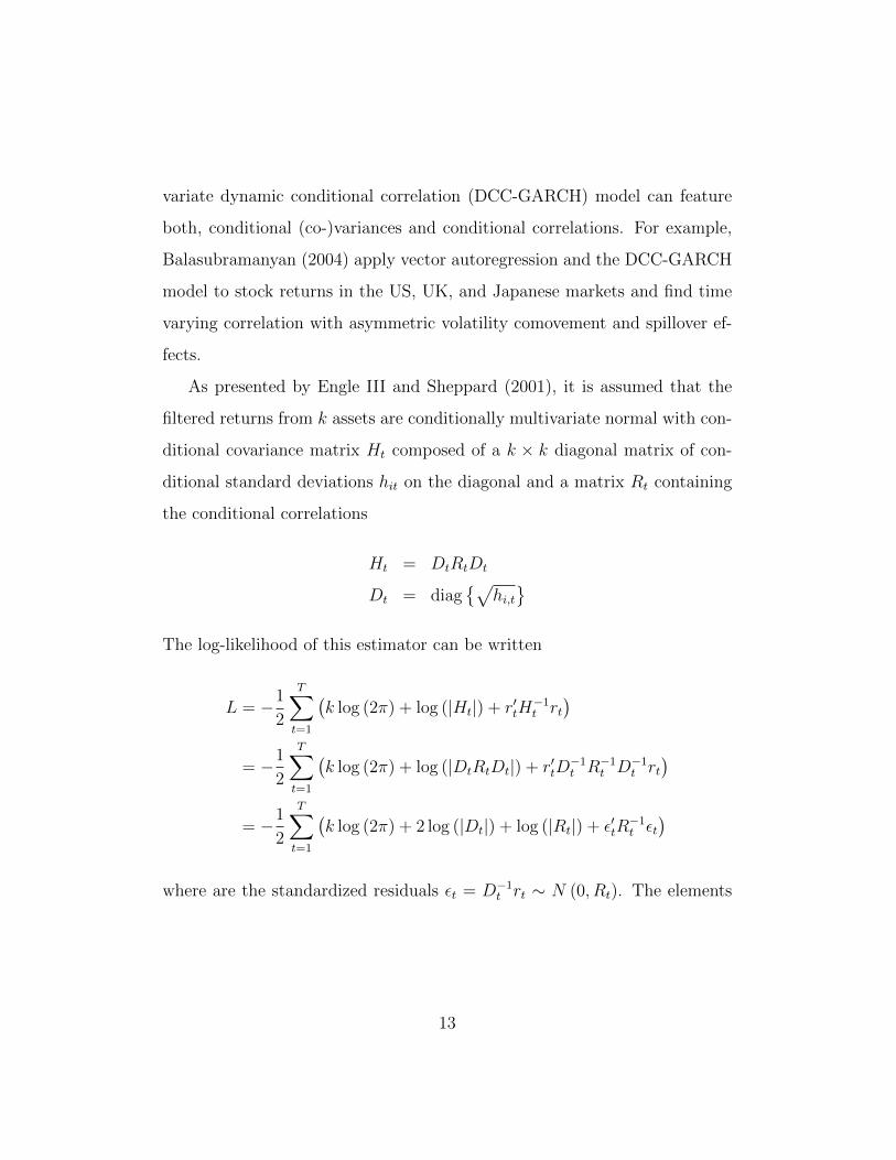
As presented by Engle III and Sheppard (2001), it is assumed that the

filtered returns from k assets are conditionally multivariate normal with con-

ditional covariance matrix Ht composed of a k × k diagonal matrix of con-

ditional standard deviations hit on the diagonal and a matrix Rt containing

the conditional correlations

Ht = DtRtDt

Dt = diag{√

hi,t}

The log-likelihood of this estimator can be written

L = −1

2

T∑t=1

(k log (2π) + log (|Ht|) + r′tH

−1t rt

)= −1

2

T∑t=1

(k log (2π) + log (|DtRtDt|) + r′tD

−1t R−1t D−1t rt

)= −1

2

T∑t=1

(k log (2π) + 2 log (|Dt|) + log (|Rt|) + ε′tR

−1t εt

)where are the standardized residuals εt = D−1t rt ∼ N (0, Rt). The elements

13

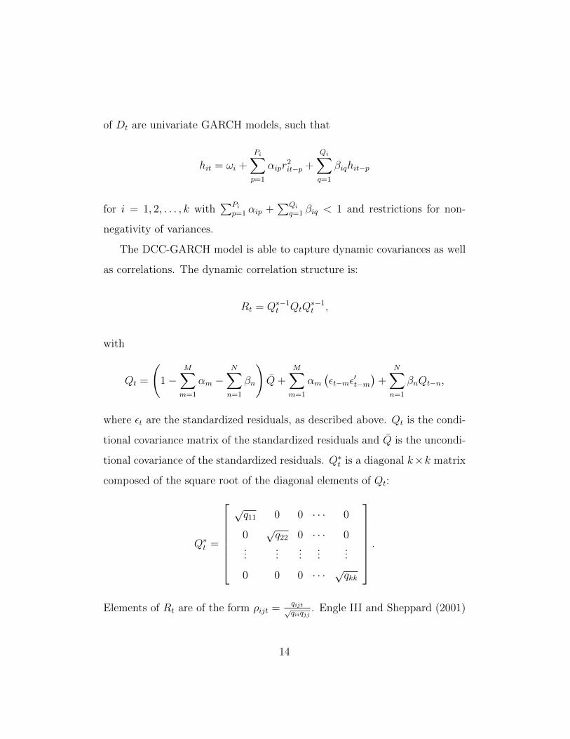
of Dt are univariate GARCH models, such that

hit = ωi +

Pi∑p=1

αipr2it−p +

Qi∑q=1

βiqhit−p

for i = 1, 2, . . . , k with∑Pi

p=1 αip +∑Qi

q=1 βiq < 1 and restrictions for non-

negativity of variances.

The DCC-GARCH model is able to capture dynamic covariances as well

as correlations. The dynamic correlation structure is:

Rt = Q∗−1t QtQ∗−1t ,

with

Qt =

(1−

M∑m=1

αm −N∑n=1

βn

)Q+

M∑m=1

αm(εt−mε

′t−m)

+N∑n=1

βnQt−n,

where εt are the standardized residuals, as described above. Qt is the condi-

tional covariance matrix of the standardized residuals and Q is the uncondi-

tional covariance of the standardized residuals. Q∗t is a diagonal k×k matrix

composed of the square root of the diagonal elements of Qt:

Q∗t =

√q11 0 0 · · · 0

0√q22 0 · · · 0

......

......

...

0 0 0 · · · √qkk

.

Elements of Rt are of the form ρijt =qijt√qiiqjj

. Engle III and Sheppard (2001)

14

show that Rt is positive definite if a number of parameter restrictions are

satisfied for all asset series i ∈ [1, . . . , k] and they develop a procedure for

estimation which this work relies on.

Engle III and Sheppard (2001) develop a test for constant correlation of

residuals of two univariate GARCH processes, i.e. H0 : Rt = R. First of all,

univariate GARCH processes are estimated and residuals are standardized.

Then the correlation of the standardized residuals is estimated. The vector of

standardized residuals is now jointly standardized by the symmetric square

root decomposition of the estimated correlation. The outer product of the

resulting residuals is then regressed on a constant and lagged outer products.

Under the null, all of the lagged parameters and the constant should be zero.

15

4. Data

For an analysis of comovement between equity markets and foreign ex-

change, the selection of data suffers from a trade-off between available number

of free floating exchange rates and time series length. Less strict requirements

on time series length imply availability of more free floating exchange rates.

This work focuses on equity market and exchange rate comovement from

January 1999 on due to two main reasons. Firstly, 1999 was the year of the

introduction of the EUR currency. From its beginnings on, it was the world’s

second most traded currency and it should have an appropriate weight in this

study. Secondly, the number of exchange rates, which are free floating, did

not substantially increase since 1999. Most of the monetary regime changes

took part before that time.

The authors are indebted to the Chair of Financial Engineering and

Derivatives (2011) at the Karlsruhe Institute of Technology for providing

access to the Bloomberg data repository. Data consist of exchange rates and

MSCI Country Indices of 30 countries. The countries have been selected due

to availability of a country index and their exchange rate regime. Countries

with managed floating with no predetermined path for the exchange rate and

countries with independently floating exchange rate arrangements, as stated

in the reports of the IMF (2004) and the IMF (2009), have been considered,

if a country index is available at the time of writing.

Most of the world’s leading currencies fulfill the floating requirement

noted above. Of the 33 currencies that contribute more than 0.1% to the

global foreign exchange market turnover, only HKD, RUB, DKK, HUF,

CNY, and SAR do not or did not have floating exchange rates for most

16

of the period of concern. HKD, CNY, and SAR have arrangements where

the USD serves as exchange rate anchor. The RUB has a fixed peg arrange-

ment to a composite of currencies and the DKK is pegged to the EUR. The

HUF is freely floating now but it did have a flexible peg to the EUR until

02/25/2008 (MNB, 2008) and therefore is not examined.

All currency exchange rates examined are local currency/USD. All MSCI

Country Indices are performance indices, which means they indicate equity

price returns and dividend yields. The indices are capitalization-weighted

and free float adjusted. All indices are denominated in local currency. Data

consist of daily observations for all trading days. Each day, the last prices of

the respective markets are taken. For foreign exchange, which is traded 24

hours a day in the interbank market, the last prices in New York at 17:00

ET (23:00 ECT) are considered relevant. At this time, all equity markets

regarded are closed and there is no overlapping. Only the following currencies

have pricing hours limited to local market hours: Brazilian real (last price

at 23:00 ECT), Chilean peso (19:30 ECT), Colombian peso (20:00 ECT),

Egyptian pound (14:30 ECT), Indonesian rupiah (11:00 ECT), Israeli shekel

(22:00 ECT), Indian rupee (13:30 ECT), South Korean won (8:00 ECT),

Malaysian ringgit (11:00 ECT), Peruvian nuevo sol (20:30 ECT), Philippine

peso (11:00 ECT), Pakistani rupee (14:30 ECT), Turkish lira (23:00 ECT),

and New Taiwan dollar (10:00 ECT).

Examining the comovement between country indices and foreign exchange

is favorable to examining the comovement of single stocks and foreign ex-

change rates for different reasons. Country Indices are not only easier to

handle in terms of data processing. The MSCI Country Indices also give a

17

general overview by comprising every listed stock in the respective market.

They cover all sectors and are not affected by mergers and acquisitions or

stock splits. Moreover, there is no apparent downside of using country indices

in a general work like this one.

The use of MSCI Country Indices comes with several advantages in terms

of comparability, since the indices are all generated by the same methodol-

ogy. Daily data is available for all markets of interest and is examined in

the period 01/01/1999–06/30/2011 with the exception of the markets of the

United Kingdom, Brazil, Turkey, and Malaysia. In the United Kingdom daily

country index data is only availably for the period 05/30/2002–04/29/2011.

Brazil’s currency has been independently floating only from 01/18/1999 on

(Meirelles, 2009) and Turkey’s from 02/28/2001 on (Gormez and Yilmaz,

2007). Malaysia’s managed floating exchange rate regime was not in place

until 05/21/2005 (BNM, 2005).

Since all currency exchange rate are equal to the local currency’s value

in USD, it is not meaningful to study the comovement between the USD,

which of course always has the value 1, and United States equities. Instead,

comovement is examined between the United States equity market and a

weighted average of a basket of exchange rates. More precisely, the exchange

rates USD/EUR (weighting 0.405), USD/JPY (0.235), USD/GBP (0.160),

USD/AUD (0.077), USD/CHF (0.064), and USD/CAD (0.060) make up the

composite exchange rate, for which comovement of United States equities

and foreign exchange is evaluated. Weightings are according to the respec-

tive average proportions in USD of foreign exchange turnover in accordance

with the Bank of International Settlement’s central bank surveys of 2001,

18

2004, 2007, and 2010 (BIS, 2010). The currencies selected are the six most

frequently traded currencies in exchange for USD. In the period regarded

they make up 80% of the foreign exchange of USD. Also, these six respective

markets and the United States market will be referred to as “major” markets

from here on, all other markets are considered “minor”.

19

5. Results

The methods established above are applied to each country separately,

considering equity market and exchange rate returns. For the United States,

the composite exchange rate USD/CMP is used instead of a single exchange

rate. Results for Egypt and Pakistan are not meaningful because of strong

non-market manipulation and therefore are not discussed.

5.1. Correlation Analysis and Linear Regression

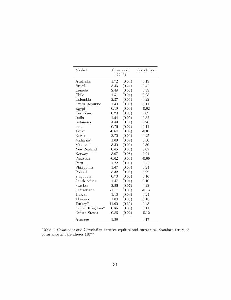
As can be seen from Table 1, correlation analysis reveals that equity

markets and foreign exchange rates are not independent. However, results

are mixed. There are positive correlations as well as negative ones. With

Egypt and Pakistan left out, the markets with positive correlation outnumber

the ones with negative correlation 25 to 3. The average correlation is slightly

positive with a value of 0.17. The absolutely strongest positive correlation of

0.43 is obtained for the Turkish market. The strongest negative correlation

of -0.13 is given by Switzerland.

There are three markets with negative correlations to the correspond-

ing exchange rates, namely the United States market, the Japanese Market

and the Swiss market. Interpretation for negative correlation of Japan and

Switzerland with their respective exchange rates is not trivial. Both exchange

rates appreciate strongly during the regarded period. This is also true for

the Swiss equity market.

A reasonable explanation is that some currencies serve as a “safe haven”

for investors in uncertain times. As equity markets decline, investors re-

allocate their funds into allegedly save currencies. Moreover, Japan’s and

20

Switzerland’s balances of trade traditionally show a surplus, which points

out the relative dependency on exports of these countries. Weak currencies

of course strengthen the competitiveness. In the case of the United States,

the economy has had a trade deficit during the whole period of concern ex-

plaining the negative relationship during strong market periods.

All other markets show positive correlation with their respective exchange

rates of varying magnitude. The Euro Zone market shows, with a value

of 0.02, the least absolute correlation of all markets regarded (leaving out

Pakistan). Other major markets, such as Australia and especially Canada

show relatively strong positive correlation with their exchange rates, just like

most minor markets.

Beside the fact that the major markets have comparably small correla-

tions, economic development does not have a unique influence on the corre-

lation. For example, the two emerging markets of South Africa and Turkey

display correlation close to zero as well as, on the other hand, very high cor-

relation. Geographical proximity is also not relevant. The South East Asian

markets of Thailand and Malaysia for example show quite different correla-

tions. However, it is apparent that correlation in the Americas markets is

comparably high with an average correlation of 0.29.

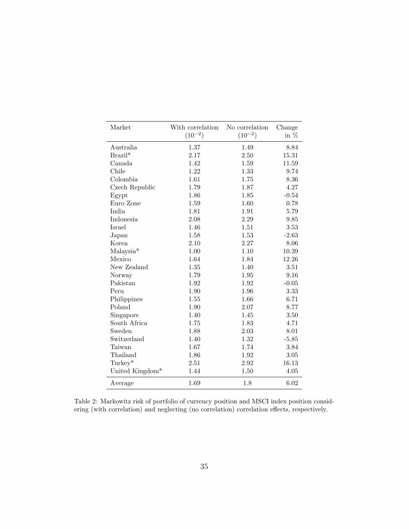
To demonstrate the effect on the portfolio risk, in Table 2 we display

Markowitz’s risk measure of portfolios consisting of two assets, for each mar-

ket, one being the local currency and the other an equity investment copying

the respective MSCI index. The table exhibits risk without correlation ef-

fects, risk with correlation effects, and the percentage change.

On average, investments are more than 6% riskier if correlations are con-

21

sidered. The greatest increase is above 16% in the case of a foreign investment

in Turkey. On the other hand, negative correlation between Swiss equity

market returns and CHF/USD exchange rate returns actually reduce risk for

foreign investments in Switzerland. The change in risk is directly related to

the correlation between the two assets.

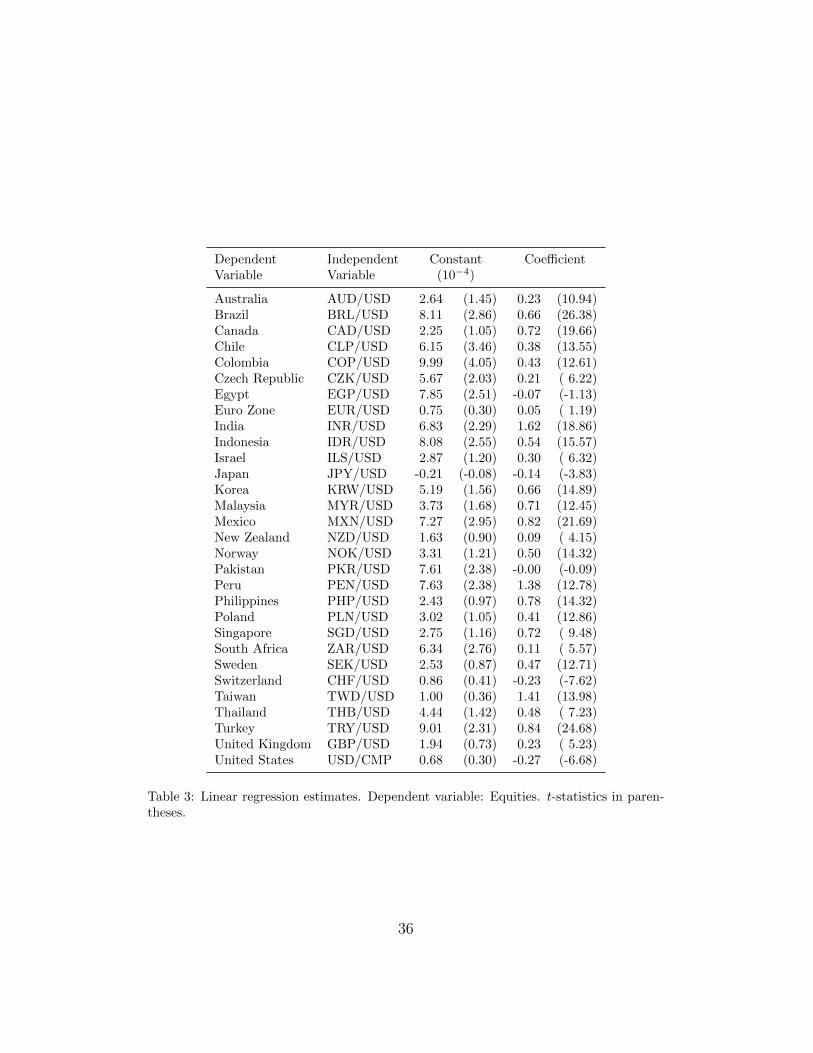
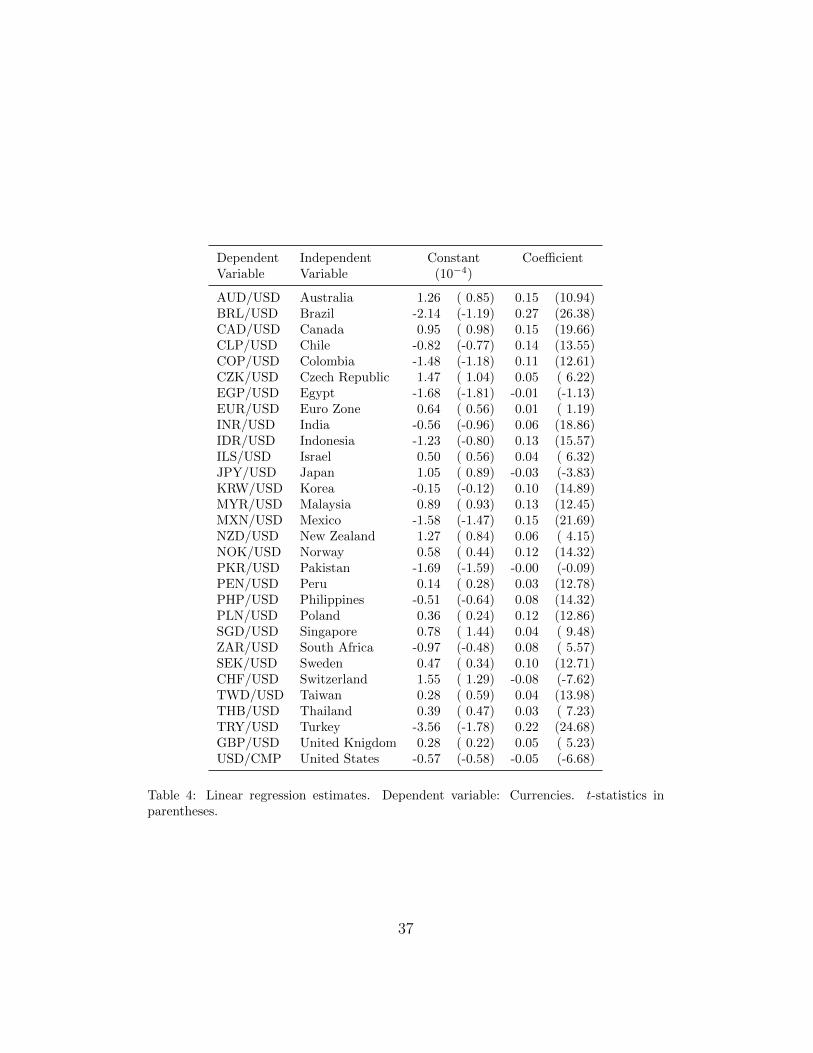
Tables 3 and 4 display the results of linear regression analysis with equity

market and exchange rates as dependent variables, respectively. The con-

stant terms are not particularly meaningful and in many case statistically

insignificant.

All regression coefficients, except for the Euro Zone market, are signifi-

cant, as t-statistics prove.4

The β coefficients are generally higher in regressions of equity markets on

exchange rates than vice versa due to higher equity market volatility.

In accordance with the correlation coefficients, only the United States’,

the Japanese, and the Swiss equity market and exchange rate coefficients

are negative. Minor markets tend to have greater regression coefficients.

Canada and Australia stick out from the major markets with comparably

high regressions coefficients. On the other hand, the markets in the Czech

Republic, South Africa, Israel, New Zealand, and Thailand have relatively

weak linear ties between their equity markets and exchange rate returns.

5.2. Vector Autoregression and Granger Causality

For each equity market and corresponding exchange rate, a vector autore-

gressive model as in equation 3.2 is employed. Without Egypt and Pakistan,

4Regression analyses for Egypt and Pakistan are not discussed due to known reasons.

22

there are 28 relevant vector autoregressions left. Since each vector contains

two variables, there are 56 regression models overall. According to the BIC

criterion, in 52 out of 56 relevant regressions, the preferable lag length is l = 1

compared to lengths of 2, 3, 4, 5, and 10. Therefore, all vector autoregressions

are conducted with l = 1.

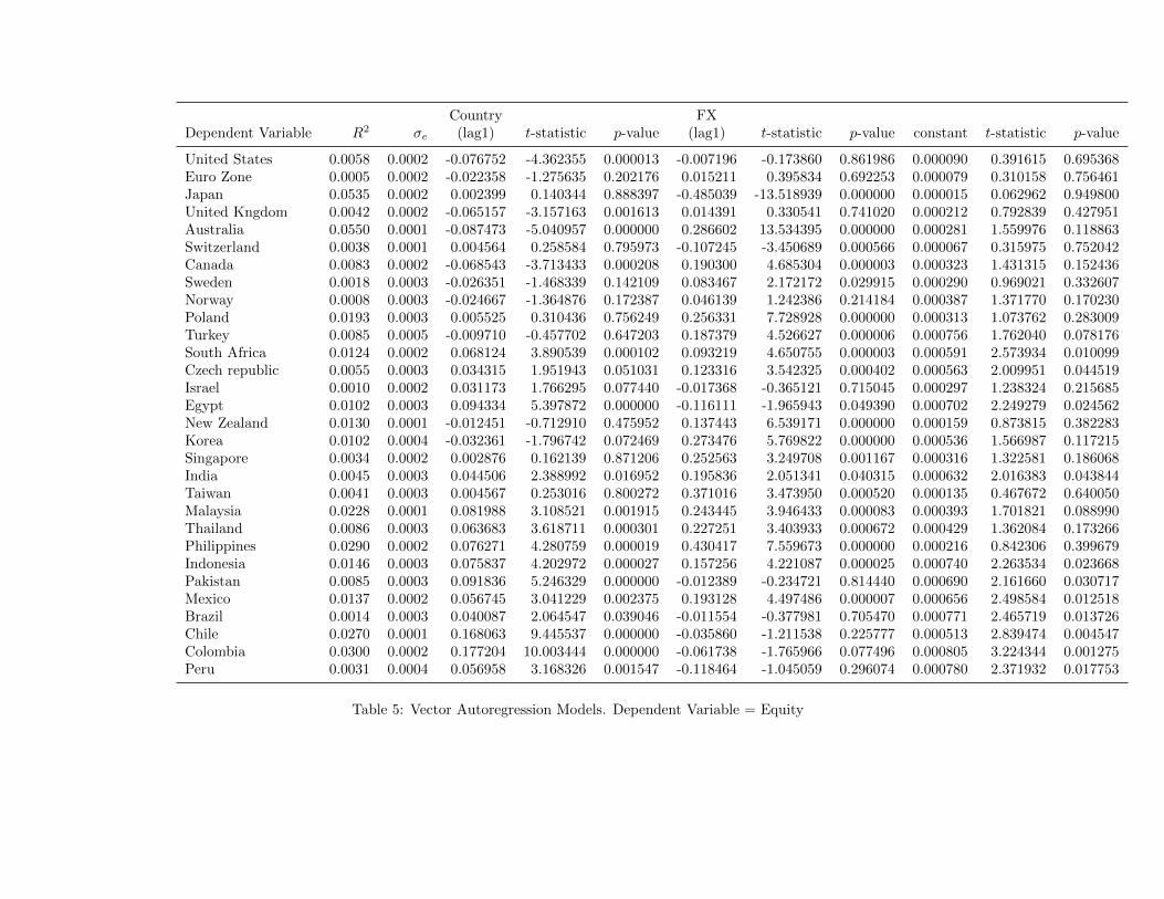
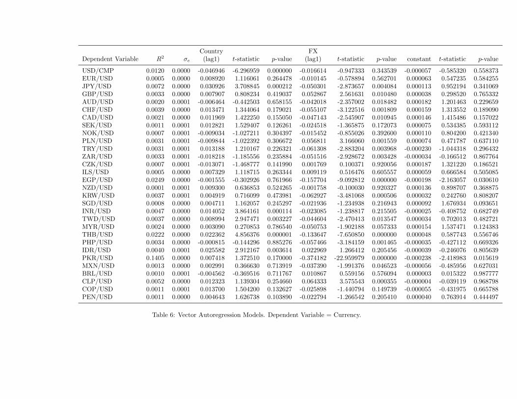
Estimation results are presented in Table 5 and 6. For every vector autore-

gression, there are two regression functions, one for each dependent variable.

For each regression, the first lags (lag1) of both equity market (country) and

exchange rate (FX) returns serve as independent variables. In Table ??, we

present the Granger test results.

The results of vector autoregression analysis and Granger causality tests

are mixed. The vector autoregressive model fit in terms of R2 is better than

the linear regression model fit in eight out of 56 cases. For five of the seven

models for the major markets, the fit is better than for the corresponding

linear regression models. This means that the vector autoregressive models

perform particularly better for the major markets since five out of eight R2

improvements overall do occur here. These are the two vector autoregressions

of the Euro Zone and Japan as well as the equity market vector autoregression

of Australia.

When interpreting these results, one has to consider the time shifts be-

tween the different markets. The exchange rate trading day ends for most

currencies at 5pm EST (New York). This is fourteen hours after closing of

the Tokyo Stock Exchange in Japan. Therefore, in the Japanese case, ex-

change rate returns of time time t contain more advanced information than

equity market returns of time t. The same is true for most currencies to

23

some extent. Even currencies which are only traded locally contain more

advanced information because interbank trading outlasts exchange trading.

Nevertheless, exchange rate returns of time t−1 precede the equity exchange

opening on day t in any case. Therefore, they may be used to predict returns

on day t.

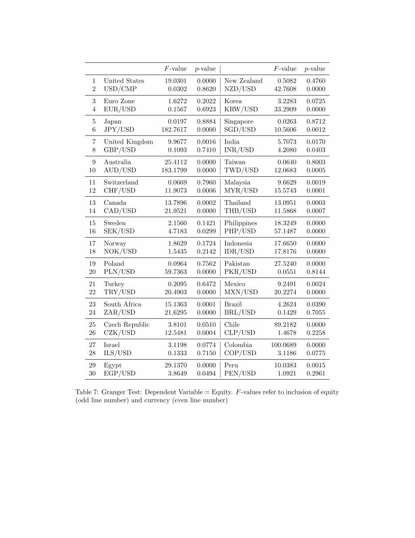
The Granger causality results vary as seen in Tables 7 and 8. Only some

series show Granger causality while others display Granger causality for one

dependent variable and not for the other. Again, in some cases, only lagged

values of the dependent variable Granger cause the process, in some cases

only the independent variable does.

Regarding the 28 relevant vector autoregressive models with equity mar-

ket returns as dependent variable (Table 7), at a significance level of 5%,

14 of them show significant auto causation and 19 show significant exchange

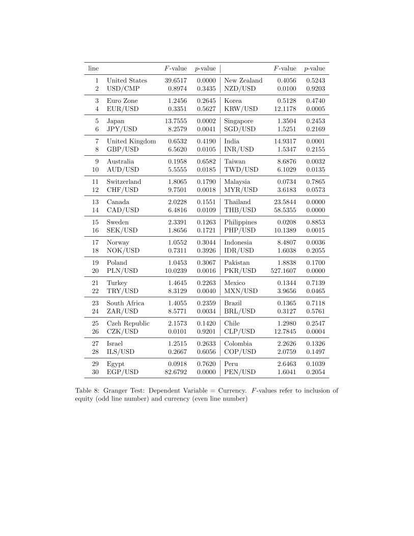
rate return causation. Of the 28 vector autoregressive models with the ex-

change rate returns as dependent variable (Table 8), 14 show significant auto

causation and 6 show significant equity market return causation. Thus, over-

all, exchange rate returns are more influential in terms of Granger causation

than equity market returns.

5.3. Geweke Measure

For computability, 20 lags were used. The instantaneous feedback mea-

sures are different from the instantaneous measures presented above in so far

that vector autoregressive effects are subtracted.

The Geweke measures consolidate the results above, as one can see in

table 9. They tend to exhibit strong linear dependence for the same eq-

uity markets and exchange rates which exhibit strong correlation or Granger

24

causality. In addition to that, the analysis contributes a differentiated view

on linear dependence, since lagged and instantaneous factors are singled out.

The analysis underlines once again that by tendency, the instantaneous link-

ages between equity markets and exchange rates are stronger than single

lagged linkages. In 19 out of 28 relevant relationships, this is true. In the

other nine cases, a single lagged feedback is stronger, mostly currency feed-

back. Moreover, currency feedback is generally stronger than market feed-

back. This underlines the results from Granger causality analysis, that lagged

currency market returns are more influential on equity market returns than

vice versa.

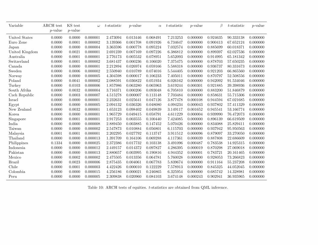
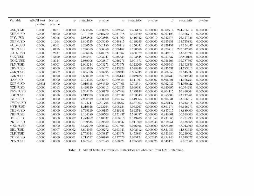
5.4. Dynamic Conditional Correlation GARCH

First, for each univariate series, Engle’s test for ARCH effects (Engle,

1982) and a Kolmogorov-Smirnov test for normality of model residuals has

been performed, and resulting p-values are displayed in Table 10 (equities)

and 11 (exchange rates), respectively.5

Notably, no equity return series fulfills the assumption of residual nor-

mality. The Kolmogorov-Smirnov test for normality is rejected at the 5%

significance level in every single case. The results for the exchange rate re-

turn series are not as clear cut. Nevertheless, normality is rejected for the

large majority. In 23 out of 28 cases, the Kolmogorov-Smirnov test rejects a

normal distribution at the 5% significance level.

The tests for no ARCH effects confirm the presence of volatility clustering.

Only in one case, it is not possible to reject the hypothesis of no ARCH effects

5Computations in this subsection are based on Matlab code provided by http://www.

kevinsheppard.com/wiki/UCSD_GARCH.

25

at the 5% significance level. The tests for constant correlation on the other

hand are somewhat ambiguous. Constant correlation can only be rejected in

eight cases at the 5% significance level.

All univariate GARCH models have in common that the constant terms

ω are very small compared to the unconditional variance. Unconditional

variances have magnitudes of 10−5 to 10−4, whereas the ωs have magnitudes

of only 10−7 to 10−6. The ω coefficient is significantly smaller than the α

coefficient in every case. Therefore, lagged returns have greater impact on

volatility than the unconditional term. Still, ω is significantly different from

zero in most cases. Especially the univariate GARCH exchange rate return

models hold significant constant terms.

However, most influential is the autoregressive term of the volatility

model. The β coefficient is larger than the ω and α coefficients for every

series. The β is responsible for a long memory property of the conditional

variance process. Many series have a β close to one and therefore exhibit

very long memory.6

For all pairs of equity market and exchange rate return data, bivariate

estimation of the DCC(1,1)-GARCH(1,1) model has been conducted. The

results are displayed in Table 12.7 Moreover, the results of the test for

dynamic correlation and the log likelihood at the optimum are displayed.

For the DCC, a simple first order model with lag lengths P = 1, Q = 1 is

selected in accordance with Engle (2002). The BIC results for the univariate

6The coefficient β can of course not be equal to or greater than one, since this wouldimply a unit root and therefore infinite variance.

7Even though returns are not normal, quasi-maximum likelihood as mentioned in (En-gle, 2002) provides for consistent estimators.

26

GARCH models vary. The criterion actually suggests a GARCH(0,1) model

in most cases. However, the transient factor α of the prior period returns

is meaningful, in some cases. For consistency, the DCC(1,1)-GARCH(1,1)

model is selected throughout. Then, elements qi,j,t of Qt in equation 3.4 take

the following form for equity return series y1,t and exchange rate return series

y2,t

qi,j,t = (1− α− β) qi,j + α (εi,t−1εj,t−1) + βqi,j,t−1

for i, j ∈ {1, 2}. The constant term q1,2 is the unconditional correlation

between the standardized returns. Therefore, for general i and j,

ρi,j,t =qi,j,t√qi,i,tqj,j,t

.

For the conditional correlation processes, the α are close to zero, whereas

the β are mostly close to one. Thus, correlation processes tend to have

very long memory. This tendency is more pronounced than in the univariate

conditional volatility models. Although the α are small in each case, they

are still mostly significant at a 5% level.8

Regarding the major markets, results are mixed, once again. The hypoth-

esis of constant correlation is rejected for the United States market, the Euro

Zone market, and the Canadian market at the 5% level. For Australia, Japan,

and Switzerland, the hypothesis of constant correlation cannot be rejected.

Of the developing markets, in our sample, only Chile and South Africa have

significant instability in their respective correlations between equity returns

8The corresponding t-values are obtained using equation (33) in Engle (2002).

27

and exchange rates. So, it appears as if comovement as measured by corre-

lation is of particularly stable nature in developing countries. A hypothesis

would be that this is the results since neither of them provides currency safe

havens nor are their markets self-sustainable enough to be less dependent on

the international currency exchange rates.

28

6. Conclusion

We saw that comovement was detected in many cases. Several differ-

ent methodologies of comovement measurement were applied often yielding

mixed results. Therefore, the importance of the sensitivity of comovement

to the measurement technique was emphasized.

Correlations between equity market and exchange rate returns were shown

to have impact on the risk foreign investors are exposed to. In particular,

we demonstrated that according to the Markowitz’s measure, risk will be 6%

higher on average, if this study’s correlations are considered.

This study provided a comprehensive approach to document comovement

between equity markets and foreign exchange on a global scale. It focused

on the most common techniques used in available comovement research to

analyze comovement at level scale as well as the inherent dynamics.

It appeared that regional clusters had not necessarily influence on the level

of comovement between foreign exchange rates and equity returns except for,

maybe, in Latin America.

Moreover, we challanged the assumption that the relationships between

equity markets and foreign exchange are stable. Fundamentals change, mon-

etary policies change, investors change. Why should the relationship between

equity market and exchange rate returns not change? We found that this

relationship was particularly instable in developed economies compared to

developing economies.

Furthermore, the examination period can be extended for some currencies

back to the collapse of the Bretton Woods system in 1971.

In international investmnts, the comovement of equity and foreign ex-

29

change rates play an essential role for risk assessment.

30

7. Appendix

31

Short form MeaningAUD Australian dollarARCH autoregressive conditional heteroscedasticityBRL Brazilian realCAC French stock market indexCAD Canadian dollarCHF Swiss francCLP Chilean PesoCOP Colombian PesoCMP Weighted composite of EUR, JPY, GBP, AUD, CHF, CADCZK Czech korunaDCC dynamic conditional correlationDEM Deutsche MarkEGP Egyptian poundEMEA Europe, Middle East, and AfricaEUR EuroFRF French francGARCH generalized autoregressive conditional heteroscedasticityGBP Pound sterlingIDR Indonesian rupiahILS Israeli new shekelINR Indian rupeeJPY Japanese yenKRW South Korean wonMXN Mexican pesoMYR Malaysian ringgitNOK Norwegian kroneNZD New Zealand dollarPEN Peruvian nuevo solPHP Philippine pesoPKR Pakistani rupeePLN Polish z lotySEK Swedish kronaSGD Singapore dollarTHB Thai bahtTRY Turkish liraTWD New Taiwan dollarZAR South African rand

32

0.8

0.9

1

1.1

1.2

1.3

1.4

1.5

1.6

Exc

hang

e R

ate

1999 2000 2001 2002 2003 2004 2005 2005 2007 2008 2009 2010 2011400

600

800

1000

1200

1400

1600

1800

2000

2200

Equ

ity In

dex

EUR/USD

Euro Zone USDEuro Zone EUR

Figure 1: MSCI Euro Index Performance and EUR/USD Exchange Rate

33

Market Covariance Correlation(10−5)

Australia 1.72 (0.04) 0.19Brazil* 8.43 (0.21) 0.42Canada 2.48 (0.06) 0.33Chile 1.51 (0.04) 0.23Colombia 2.27 (0.06) 0.22Czech Republic 1.40 (0.03) 0.11Egypt -0.19 (0.00) -0.02Euro Zone 0.20 (0.00) 0.02India 1.94 (0.05) 0.32Indonesia 4.49 (0.11) 0.26Israel 0.76 (0.02) 0.11Japan -0.64 (0.02) -0.07Korea 3.70 (0.09) 0.25Malaysia* 1.09 (0.04) 0.30Mexico 3.50 (0.09) 0.36New Zealand 0.65 (0.02) 0.07Norway 3.07 (0.08) 0.24Pakistan -0.02 (0.00) -0.00Peru 1.22 (0.03) 0.22Philippines 1.67 (0.04) 0.24Poland 3.32 (0.08) 0.22Singapore 0.70 (0.02) 0.16South Africa 1.47 (0.04) 0.10Sweden 2.96 (0.07) 0.22Switzerland -1.11 (0.03) -0.13Taiwan 1.10 (0.03) 0.24Thailand 1.08 (0.03) 0.13Turkey* 11.00 (0.30) 0.43United Kingdom* 0.86 (0.02) 0.11United States -0.86 (0.02) -0.12

Average 1.99 0.17

Table 1: Covariance and Correlation between equities and currencies. Standard errors ofcovariance in parentheses (10−5)

34

Market With correlation No correlation Change(10−2) (10−2) in %

Australia 1.37 1.49 8.84Brazil* 2.17 2.50 15.31Canada 1.42 1.59 11.59Chile 1.22 1.33 9.74Colombia 1.61 1.75 8.36Czech Republic 1.79 1.87 4.27Egypt 1.86 1.85 -0.54Euro Zone 1.59 1.60 0.78India 1.81 1.91 5.79Indonesia 2.08 2.29 9.85Israel 1.46 1.51 3.53Japan 1.58 1.53 -2.63Korea 2.10 2.27 8.06Malaysia* 1.00 1.10 10.39Mexico 1.64 1.84 12.26New Zealand 1.35 1.40 3.51Norway 1.79 1.95 9.16Pakistan 1.92 1.92 -0.05Peru 1.90 1.96 3.33Philippines 1.55 1.66 6.71Poland 1.90 2.07 8.77Singapore 1.40 1.45 3.50South Africa 1.75 1.83 4.71Sweden 1.88 2.03 8.01Switzerland 1.40 1.32 -5.85Taiwan 1.67 1.74 3.84Thailand 1.86 1.92 3.05Turkey* 2.51 2.92 16.13United Kingdom* 1.44 1.50 4.05

Average 1.69 1.8 6.02

Table 2: Markowitz risk of portfolio of currency position and MSCI index position consid-ering (with correlation) and neglecting (no correlation) correlation effects, respectively.

35

Dependent Independent Constant CoefficientVariable Variable (10−4)

Australia AUD/USD 2.64 (1.45) 0.23 (10.94)Brazil BRL/USD 8.11 (2.86) 0.66 (26.38)Canada CAD/USD 2.25 (1.05) 0.72 (19.66)Chile CLP/USD 6.15 (3.46) 0.38 (13.55)Colombia COP/USD 9.99 (4.05) 0.43 (12.61)Czech Republic CZK/USD 5.67 (2.03) 0.21 ( 6.22)Egypt EGP/USD 7.85 (2.51) -0.07 (-1.13)Euro Zone EUR/USD 0.75 (0.30) 0.05 ( 1.19)India INR/USD 6.83 (2.29) 1.62 (18.86)Indonesia IDR/USD 8.08 (2.55) 0.54 (15.57)Israel ILS/USD 2.87 (1.20) 0.30 ( 6.32)Japan JPY/USD -0.21 (-0.08) -0.14 (-3.83)Korea KRW/USD 5.19 (1.56) 0.66 (14.89)Malaysia MYR/USD 3.73 (1.68) 0.71 (12.45)Mexico MXN/USD 7.27 (2.95) 0.82 (21.69)New Zealand NZD/USD 1.63 (0.90) 0.09 ( 4.15)Norway NOK/USD 3.31 (1.21) 0.50 (14.32)Pakistan PKR/USD 7.61 (2.38) -0.00 (-0.09)Peru PEN/USD 7.63 (2.38) 1.38 (12.78)Philippines PHP/USD 2.43 (0.97) 0.78 (14.32)Poland PLN/USD 3.02 (1.05) 0.41 (12.86)Singapore SGD/USD 2.75 (1.16) 0.72 ( 9.48)South Africa ZAR/USD 6.34 (2.76) 0.11 ( 5.57)Sweden SEK/USD 2.53 (0.87) 0.47 (12.71)Switzerland CHF/USD 0.86 (0.41) -0.23 (-7.62)Taiwan TWD/USD 1.00 (0.36) 1.41 (13.98)Thailand THB/USD 4.44 (1.42) 0.48 ( 7.23)Turkey TRY/USD 9.01 (2.31) 0.84 (24.68)United Kingdom GBP/USD 1.94 (0.73) 0.23 ( 5.23)United States USD/CMP 0.68 (0.30) -0.27 (-6.68)

Table 3: Linear regression estimates. Dependent variable: Equities. t-statistics in paren-theses.

36

Dependent Independent Constant CoefficientVariable Variable (10−4)

AUD/USD Australia 1.26 ( 0.85) 0.15 (10.94)BRL/USD Brazil -2.14 (-1.19) 0.27 (26.38)CAD/USD Canada 0.95 ( 0.98) 0.15 (19.66)CLP/USD Chile -0.82 (-0.77) 0.14 (13.55)COP/USD Colombia -1.48 (-1.18) 0.11 (12.61)CZK/USD Czech Republic 1.47 ( 1.04) 0.05 ( 6.22)EGP/USD Egypt -1.68 (-1.81) -0.01 (-1.13)EUR/USD Euro Zone 0.64 ( 0.56) 0.01 ( 1.19)INR/USD India -0.56 (-0.96) 0.06 (18.86)IDR/USD Indonesia -1.23 (-0.80) 0.13 (15.57)ILS/USD Israel 0.50 ( 0.56) 0.04 ( 6.32)JPY/USD Japan 1.05 ( 0.89) -0.03 (-3.83)KRW/USD Korea -0.15 (-0.12) 0.10 (14.89)MYR/USD Malaysia 0.89 ( 0.93) 0.13 (12.45)MXN/USD Mexico -1.58 (-1.47) 0.15 (21.69)NZD/USD New Zealand 1.27 ( 0.84) 0.06 ( 4.15)NOK/USD Norway 0.58 ( 0.44) 0.12 (14.32)PKR/USD Pakistan -1.69 (-1.59) -0.00 (-0.09)PEN/USD Peru 0.14 ( 0.28) 0.03 (12.78)PHP/USD Philippines -0.51 (-0.64) 0.08 (14.32)PLN/USD Poland 0.36 ( 0.24) 0.12 (12.86)SGD/USD Singapore 0.78 ( 1.44) 0.04 ( 9.48)ZAR/USD South Africa -0.97 (-0.48) 0.08 ( 5.57)SEK/USD Sweden 0.47 ( 0.34) 0.10 (12.71)CHF/USD Switzerland 1.55 ( 1.29) -0.08 (-7.62)TWD/USD Taiwan 0.28 ( 0.59) 0.04 (13.98)THB/USD Thailand 0.39 ( 0.47) 0.03 ( 7.23)TRY/USD Turkey -3.56 (-1.78) 0.22 (24.68)GBP/USD United Knigdom 0.28 ( 0.22) 0.05 ( 5.23)USD/CMP United States -0.57 (-0.58) -0.05 (-6.68)

Table 4: Linear regression estimates. Dependent variable: Currencies. t-statistics inparentheses.

37

Country FXDependent Variable R2 σe (lag1) t-statistic p-value (lag1) t-statistic p-value constant t-statistic p-value

United States 0.0058 0.0002 -0.076752 -4.362355 0.000013 -0.007196 -0.173860 0.861986 0.000090 0.391615 0.695368Euro Zone 0.0005 0.0002 -0.022358 -1.275635 0.202176 0.015211 0.395834 0.692253 0.000079 0.310158 0.756461Japan 0.0535 0.0002 0.002399 0.140344 0.888397 -0.485039 -13.518939 0.000000 0.000015 0.062962 0.949800United Kngdom 0.0042 0.0002 -0.065157 -3.157163 0.001613 0.014391 0.330541 0.741020 0.000212 0.792839 0.427951Australia 0.0550 0.0001 -0.087473 -5.040957 0.000000 0.286602 13.534395 0.000000 0.000281 1.559976 0.118863Switzerland 0.0038 0.0001 0.004564 0.258584 0.795973 -0.107245 -3.450689 0.000566 0.000067 0.315975 0.752042Canada 0.0083 0.0002 -0.068543 -3.713433 0.000208 0.190300 4.685304 0.000003 0.000323 1.431315 0.152436Sweden 0.0018 0.0003 -0.026351 -1.468339 0.142109 0.083467 2.172172 0.029915 0.000290 0.969021 0.332607Norway 0.0008 0.0003 -0.024667 -1.364876 0.172387 0.046139 1.242386 0.214184 0.000387 1.371770 0.170230Poland 0.0193 0.0003 0.005525 0.310436 0.756249 0.256331 7.728928 0.000000 0.000313 1.073762 0.283009Turkey 0.0085 0.0005 -0.009710 -0.457702 0.647203 0.187379 4.526627 0.000006 0.000756 1.762040 0.078176South Africa 0.0124 0.0002 0.068124 3.890539 0.000102 0.093219 4.650755 0.000003 0.000591 2.573934 0.010099Czech republic 0.0055 0.0003 0.034315 1.951943 0.051031 0.123316 3.542325 0.000402 0.000563 2.009951 0.044519Israel 0.0010 0.0002 0.031173 1.766295 0.077440 -0.017368 -0.365121 0.715045 0.000297 1.238324 0.215685Egypt 0.0102 0.0003 0.094334 5.397872 0.000000 -0.116111 -1.965943 0.049390 0.000702 2.249279 0.024562New Zealand 0.0130 0.0001 -0.012451 -0.712910 0.475952 0.137443 6.539171 0.000000 0.000159 0.873815 0.382283Korea 0.0102 0.0004 -0.032361 -1.796742 0.072469 0.273476 5.769822 0.000000 0.000536 1.566987 0.117215Singapore 0.0034 0.0002 0.002876 0.162139 0.871206 0.252563 3.249708 0.001167 0.000316 1.322581 0.186068India 0.0045 0.0003 0.044506 2.388992 0.016952 0.195836 2.051341 0.040315 0.000632 2.016383 0.043844Taiwan 0.0041 0.0003 0.004567 0.253016 0.800272 0.371016 3.473950 0.000520 0.000135 0.467672 0.640050Malaysia 0.0228 0.0001 0.081988 3.108521 0.001915 0.243445 3.946433 0.000083 0.000393 1.701821 0.088990Thailand 0.0086 0.0003 0.063683 3.618711 0.000301 0.227251 3.403933 0.000672 0.000429 1.362084 0.173266Philippines 0.0290 0.0002 0.076271 4.280759 0.000019 0.430417 7.559673 0.000000 0.000216 0.842306 0.399679Indonesia 0.0146 0.0003 0.075837 4.202972 0.000027 0.157256 4.221087 0.000025 0.000740 2.263534 0.023668Pakistan 0.0085 0.0003 0.091836 5.246329 0.000000 -0.012389 -0.234721 0.814440 0.000690 2.161660 0.030717Mexico 0.0137 0.0002 0.056745 3.041229 0.002375 0.193128 4.497486 0.000007 0.000656 2.498584 0.012518Brazil 0.0014 0.0003 0.040087 2.064547 0.039046 -0.011554 -0.377981 0.705470 0.000771 2.465719 0.013726Chile 0.0270 0.0001 0.168063 9.445537 0.000000 -0.035860 -1.211538 0.225777 0.000513 2.839474 0.004547Colombia 0.0300 0.0002 0.177204 10.003444 0.000000 -0.061738 -1.765966 0.077496 0.000805 3.224344 0.001275Peru 0.0031 0.0004 0.056958 3.168326 0.001547 -0.118464 -1.045059 0.296074 0.000780 2.371932 0.017753

Table 5: Vector Autoregression Models. Dependent Variable = Equity

Country FXDependent Variable R2 σe (lag1) t-statistic p-value (lag1) t-statistic p-value constant t-statistic p-value

USD/CMP 0.0120 0.0000 -0.046946 -6.296959 0.000000 -0.016614 -0.947333 0.343539 -0.000057 -0.585320 0.558373EUR/USD 0.0005 0.0000 0.008920 1.116061 0.264478 -0.010145 -0.578894 0.562701 0.000063 0.547235 0.584255JPY/USD 0.0072 0.0000 0.030926 3.708845 0.000212 -0.050301 -2.873657 0.004084 0.000113 0.952194 0.341069GBP/USD 0.0033 0.0000 0.007907 0.808234 0.419037 0.052867 2.561631 0.010480 0.000038 0.298520 0.765332AUD/USD 0.0020 0.0001 -0.006464 -0.442503 0.658155 -0.042018 -2.357002 0.018482 0.000182 1.201463 0.229659CHF/USD 0.0039 0.0000 0.013471 1.344064 0.179021 -0.055107 -3.122516 0.001809 0.000159 1.313552 0.189090CAD/USD 0.0021 0.0000 0.011969 1.422250 0.155050 -0.047143 -2.545907 0.010945 0.000146 1.415486 0.157022SEK/USD 0.0011 0.0001 0.012821 1.529407 0.126261 -0.024518 -1.365875 0.172073 0.000075 0.534385 0.593112NOK/USD 0.0007 0.0001 -0.009034 -1.027211 0.304397 -0.015452 -0.855026 0.392600 0.000110 0.804200 0.421340PLN/USD 0.0031 0.0001 -0.009844 -1.022392 0.306672 0.056811 3.166060 0.001559 0.000074 0.471787 0.637110TRY/USD 0.0031 0.0001 0.013188 1.210167 0.226321 -0.061308 -2.883204 0.003968 -0.000230 -1.044318 0.296432ZAR/USD 0.0033 0.0001 -0.018218 -1.185556 0.235884 -0.051516 -2.928672 0.003428 -0.000034 -0.166512 0.867764CZK/USD 0.0007 0.0001 -0.013071 -1.468777 0.141990 0.001769 0.100371 0.920056 0.000187 1.321220 0.186521ILS/USD 0.0005 0.0000 0.007329 1.118715 0.263344 0.009119 0.516476 0.605557 0.000059 0.666584 0.505085EGP/USD 0.0249 0.0000 -0.001555 -0.302926 0.761966 -0.157704 -9.092812 0.000000 -0.000198 -2.163057 0.030610NZD/USD 0.0001 0.0001 0.009300 0.636853 0.524265 -0.001758 -0.100030 0.920327 0.000136 0.898707 0.368875KRW/USD 0.0037 0.0001 0.004919 0.716099 0.473981 -0.062927 -3.481068 0.000506 0.000032 0.242760 0.808207SGD/USD 0.0008 0.0000 0.004711 1.162057 0.245297 -0.021936 -1.234938 0.216943 0.000092 1.676934 0.093651INR/USD 0.0047 0.0000 0.014052 3.864161 0.000114 -0.023085 -1.238817 0.215505 -0.000025 -0.408752 0.682749TWD/USD 0.0037 0.0000 0.008994 2.947471 0.003227 -0.044604 -2.470413 0.013547 0.000034 0.702013 0.482721MYR/USD 0.0024 0.0000 0.003090 0.270853 0.786540 -0.050753 -1.902188 0.057333 0.000154 1.537471 0.124383THB/USD 0.0222 0.0000 0.022362 4.856376 0.000001 -0.133647 -7.650850 0.000000 0.000048 0.587743 0.556746PHP/USD 0.0034 0.0000 -0.000815 -0.144296 0.885276 -0.057466 -3.184159 0.001465 -0.000035 -0.427112 0.669326IDR/USD 0.0040 0.0001 0.025582 2.912167 0.003614 0.022969 1.266412 0.205456 -0.000039 -0.246076 0.805639PKR/USD 0.1405 0.0000 0.007418 1.372510 0.170000 -0.374182 -22.959979 0.000000 -0.000238 -2.418983 0.015619MXN/USD 0.0013 0.0000 0.002991 0.366630 0.713919 -0.037390 -1.991376 0.046523 -0.000056 -0.485956 0.627031BRL/USD 0.0010 0.0001 -0.004562 -0.369516 0.711767 0.010867 0.559156 0.576094 0.000003 0.015322 0.987777CLP/USD 0.0052 0.0000 0.012323 1.139304 0.254660 0.064333 3.575543 0.000355 -0.000004 -0.039119 0.968798COP/USD 0.0011 0.0001 0.013700 1.504200 0.132627 -0.025898 -1.440794 0.149739 -0.000055 -0.431975 0.665788PEN/USD 0.0011 0.0000 0.004643 1.626738 0.103890 -0.022794 -1.266542 0.205410 0.000040 0.763914 0.444497

Table 6: Vector Autoregression Models. Dependent Variable = Currency.

F -value p-value F -value p-value

1 United States 19.0301 0.0000 New Zealand 0.5082 0.47602 USD/CMP 0.0302 0.8620 NZD/USD 42.7608 0.0000

3 Euro Zone 1.6272 0.2022 Korea 3.2283 0.07254 EUR/USD 0.1567 0.6923 KRW/USD 33.2909 0.0000

5 Japan 0.0197 0.8884 Singapore 0.0263 0.87126 JPY/USD 182.7617 0.0000 SGD/USD 10.5606 0.0012

7 United Kingdom 9.9677 0.0016 India 5.7073 0.01708 GBP/USD 0.1093 0.7410 INR/USD 4.2080 0.0403

9 Australia 25.4112 0.0000 Taiwan 0.0640 0.800310 AUD/USD 183.1799 0.0000 TWD/USD 12.0683 0.0005

11 Switzerland 0.0669 0.7960 Malaysia 9.6629 0.001912 CHF/USD 11.9073 0.0006 MYR/USD 15.5743 0.0001

13 Canada 13.7896 0.0002 Thailand 13.0951 0.000314 CAD/USD 21.9521 0.0000 THB/USD 11.5868 0.0007

15 Sweden 2.1560 0.1421 Philippines 18.3249 0.000016 SEK/USD 4.7183 0.0299 PHP/USD 57.1487 0.0000

17 Norway 1.8629 0.1724 Indonesia 17.6650 0.000018 NOK/USD 1.5435 0.2142 IDR/USD 17.8176 0.0000

19 Poland 0.0964 0.7562 Pakistan 27.5240 0.000020 PLN/USD 59.7363 0.0000 PKR/USD 0.0551 0.8144

21 Turkey 0.2095 0.6472 Mexico 9.2491 0.002422 TRY/USD 20.4903 0.0000 MXN/USD 20.2274 0.0000

23 South Africa 15.1363 0.0001 Brazil 4.2624 0.039024 ZAR/USD 21.6295 0.0000 BRL/USD 0.1429 0.7055

25 Czech Republic 3.8101 0.0510 Chile 89.2182 0.000026 CZK/USD 12.5481 0.0004 CLP/USD 1.4678 0.2258

27 Israel 3.1198 0.0774 Colombia 100.0689 0.000028 ILS/USD 0.1333 0.7150 COP/USD 3.1186 0.0775

29 Egypt 29.1370 0.0000 Peru 10.0383 0.001530 EGP/USD 3.8649 0.0494 PEN/USD 1.0921 0.2961

Table 7: Granger Test: Dependent Variable = Equity. F -values refer to inclusion of equity(odd line number) and currency (even line number)

line F -value p-value F -value p-value

1 United States 39.6517 0.0000 New Zealand 0.4056 0.52432 USD/CMP 0.8974 0.3435 NZD/USD 0.0100 0.9203

3 Euro Zone 1.2456 0.2645 Korea 0.5128 0.47404 EUR/USD 0.3351 0.5627 KRW/USD 12.1178 0.0005

5 Japan 13.7555 0.0002 Singapore 1.3504 0.24536 JPY/USD 8.2579 0.0041 SGD/USD 1.5251 0.2169

7 United Kingdom 0.6532 0.4190 India 14.9317 0.00018 GBP/USD 6.5620 0.0105 INR/USD 1.5347 0.2155

9 Australia 0.1958 0.6582 Taiwan 8.6876 0.003210 AUD/USD 5.5555 0.0185 TWD/USD 6.1029 0.0135

11 Switzerland 1.8065 0.1790 Malaysia 0.0734 0.786512 CHF/USD 9.7501 0.0018 MYR/USD 3.6183 0.0573

13 Canada 2.0228 0.1551 Thailand 23.5844 0.000014 CAD/USD 6.4816 0.0109 THB/USD 58.5355 0.0000

15 Sweden 2.3391 0.1263 Philippines 0.0208 0.885316 SEK/USD 1.8656 0.1721 PHP/USD 10.1389 0.0015

17 Norway 1.0552 0.3044 Indonesia 8.4807 0.003618 NOK/USD 0.7311 0.3926 IDR/USD 1.6038 0.2055

19 Poland 1.0453 0.3067 Pakistan 1.8838 0.170020 PLN/USD 10.0239 0.0016 PKR/USD 527.1607 0.0000

21 Turkey 1.4645 0.2263 Mexico 0.1344 0.713922 TRY/USD 8.3129 0.0040 MXN/USD 3.9656 0.0465

23 South Africa 1.4055 0.2359 Brazil 0.1365 0.711824 ZAR/USD 8.5771 0.0034 BRL/USD 0.3127 0.5761

25 Czeh Republic 2.1573 0.1420 Chile 1.2980 0.254726 CZK/USD 0.0101 0.9201 CLP/USD 12.7845 0.0004

27 Israel 1.2515 0.2633 Colombia 2.2626 0.132628 ILS/USD 0.2667 0.6056 COP/USD 2.0759 0.1497

29 Egypt 0.0918 0.7620 Peru 2.6463 0.103930 EGP/USD 82.6792 0.0000 PEN/USD 1.6041 0.2054

Table 8: Granger Test: Dependent Variable = Currency. F -values refer to inclusion ofequity (odd line number) and currency (even line number)

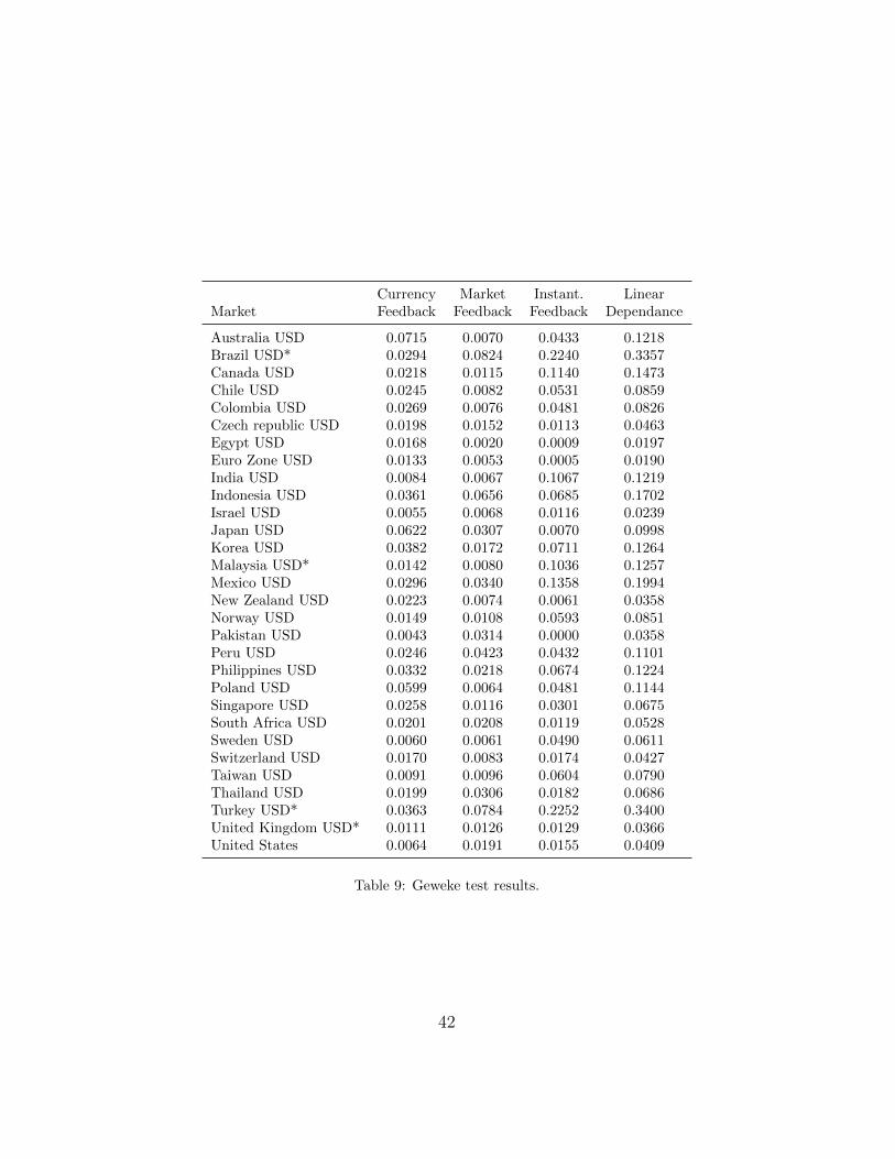
Currency Market Instant. LinearMarket Feedback Feedback Feedback Dependance

Australia USD 0.0715 0.0070 0.0433 0.1218Brazil USD* 0.0294 0.0824 0.2240 0.3357Canada USD 0.0218 0.0115 0.1140 0.1473Chile USD 0.0245 0.0082 0.0531 0.0859Colombia USD 0.0269 0.0076 0.0481 0.0826Czech republic USD 0.0198 0.0152 0.0113 0.0463Egypt USD 0.0168 0.0020 0.0009 0.0197Euro Zone USD 0.0133 0.0053 0.0005 0.0190India USD 0.0084 0.0067 0.1067 0.1219Indonesia USD 0.0361 0.0656 0.0685 0.1702Israel USD 0.0055 0.0068 0.0116 0.0239Japan USD 0.0622 0.0307 0.0070 0.0998Korea USD 0.0382 0.0172 0.0711 0.1264Malaysia USD* 0.0142 0.0080 0.1036 0.1257Mexico USD 0.0296 0.0340 0.1358 0.1994New Zealand USD 0.0223 0.0074 0.0061 0.0358Norway USD 0.0149 0.0108 0.0593 0.0851Pakistan USD 0.0043 0.0314 0.0000 0.0358Peru USD 0.0246 0.0423 0.0432 0.1101Philippines USD 0.0332 0.0218 0.0674 0.1224Poland USD 0.0599 0.0064 0.0481 0.1144Singapore USD 0.0258 0.0116 0.0301 0.0675South Africa USD 0.0201 0.0208 0.0119 0.0528Sweden USD 0.0060 0.0061 0.0490 0.0611Switzerland USD 0.0170 0.0083 0.0174 0.0427Taiwan USD 0.0091 0.0096 0.0604 0.0790Thailand USD 0.0199 0.0306 0.0182 0.0686Turkey USD* 0.0363 0.0784 0.2252 0.3400United Kingdom USD* 0.0111 0.0126 0.0129 0.0366United States 0.0064 0.0191 0.0155 0.0409

Table 9: Geweke test results.

42

Variable ARCH test KS test ω t-statistic p-value α t-statistic p-value β t-statistic p-valuep-value p-value

United States 0.0000 0.0000 0.000001 2.473094 0.013446 0.068491 7.213253 0.000000 0.924635 90.333138 0.000000Euro Zone 0.0000 0.0001 0.000002 3.139366 0.001708 0.091926 6.734647 0.000000 0.900413 67.652124 0.000000Japan 0.0000 0.0000 0.000004 3.363596 0.000778 0.095224 7.032574 0.000000 0.885699 60.018371 0.000000United Kingdom 0.0000 0.0021 0.000001 2.691239 0.007169 0.097226 6.386812 0.000000 0.899397 62.027536 0.000000Australia 0.0000 0.0001 0.000001 2.776173 0.005532 0.078951 5.652093 0.000000 0.914995 65.181342 0.000000Switzerland 0.0000 0.0001 0.000002 3.681437 0.000236 0.106020 7.375475 0.000000 0.878703 57.650235 0.000000Canada 0.0000 0.0000 0.000001 2.212894 0.026974 0.059166 5.588318 0.000000 0.936737 80.331673 0.000000Sweden 0.0000 0.0006 0.000002 2.550940 0.010789 0.074016 5.544405 0.000000 0.921203 66.865560 0.000000Norway 0.0000 0.0000 0.000005 4.304598 0.000017 0.106233 7.405011 0.000000 0.870797 52.508556 0.000000Poland 0.0000 0.0041 0.000002 2.088591 0.036822 0.051934 6.026162 0.000000 0.942092 91.534046 0.000000Turkey 0.0000 0.0103 0.000006 1.857986 0.063280 0.065963 3.619244 0.000301 0.921885 39.398936 0.000000South Afrika 0.0000 0.0032 0.000004 3.716371 0.000206 0.093048 6.705810 0.000000 0.883200 51.846879 0.000000Czeh Republic 0.0000 0.0003 0.000007 4.515278 0.000007 0.113148 7.703484 0.000000 0.858631 55.715306 0.000000Israel 0.0000 0.0000 0.000001 2.232631 0.025641 0.047126 3.877478 0.000108 0.944594 67.021685 0.000000Egypt 0.0000 0.0000 0.000005 2.094132 0.036326 0.048080 4.094234 0.000043 0.937802 57.411329 0.000000New Zealand 0.0000 0.0032 0.000001 1.653123 0.098402 0.049839 3.149117 0.001652 0.945541 53.166774 0.000000Korea 0.0000 0.0000 0.000001 1.965729 0.049415 0.058791 4.611229 0.000004 0.939990 76.472073 0.000000Singapore 0.0000 0.0001 0.000001 2.917253 0.003555 0.100440 7.424085 0.000000 0.896139 66.619509 0.000000India 0.0000 0.0000 0.000008 2.889450 0.003885 0.147452 5.070426 0.000000 0.834088 25.829411 0.000000Taiwan 0.0000 0.0000 0.000002 2.547873 0.010884 0.056801 6.115703 0.000000 0.937942 95.950563 0.000000Malaysia 0.0001 0.0001 0.000001 2.202295 0.027792 0.113747 3.911512 0.000096 0.879097 33.270050 0.000000Thailand 0.0000 0.0000 0.000013 1.391709 0.164106 0.069288 4.117361 0.000039 0.887808 22.686609 0.000000Philippines 0.1334 0.0000 0.000025 2.372386 0.017732 0.103138 3.491096 0.000487 0.783538 14.925315 0.000000Indonesia 0.0000 0.0000 0.000012 2.449157 0.014372 0.097827 4.286395 0.000019 0.870298 27.069018 0.000000Pakistan 0.0000 0.0000 0.000013 2.880657 0.003995 0.190816 4.944352 0.000001 0.783721 20.161465 0.000000Mexico 0.0000 0.0002 0.000002 2.475505 0.013356 0.064781 5.760028 0.000000 0.928053 73.266823 0.000000Brazil 0.0000 0.0023 0.000006 2.875435 0.004061 0.067783 5.839674 0.000000 0.911164 55.237208 0.000000Chile 0.0000 0.0001 0.000003 4.422426 0.000010 0.122229 7.578913 0.000000 0.845325 44.052045 0.000000Colombia 0.0000 0.0000 0.000015 4.256186 0.000021 0.246865 6.325954 0.000000 0.685742 14.328981 0.000000Peru 0.0000 0.0000 0.000005 2.309838 0.020960 0.084103 3.674148 0.000243 0.902941 36.935965 0.000000

Table 10: ARCH tests of equities. t-statistics are obtained from QML inference.

Variable ARCH test KS test ω t-statistic p-value α t-statistic p-value β t-statistic p-valuep-value p-value

USD/CMP 0.0000 0.0421 0.000000 3.638635 0.000278 0.032556 7.456173 0.000000 0.962714 244.705613 0.000000EUR/USD 0.0000 0.0602 0.000000 0.101979 0.918780 0.031078 7.424629 0.000000 0.967123 31.466714 0.000000JPY/USD 0.0000 0.0016 0.000001 2.983806 0.002868 0.041660 4.416452 0.000010 0.942475 76.127626 0.000000GBP/USD 0.0000 0.1264 0.000000 2.804525 0.005080 0.038815 6.139296 0.000000 0.955351 163.725852 0.000000AUD/USD 0.0000 0.0011 0.000001 3.246509 0.001180 0.058718 6.256042 0.000000 0.929157 89.154047 0.000000CHF/USD 0.0000 0.0195 0.000000 2.746358 0.006059 0.025187 5.720566 0.000000 0.970719 222.012605 0.000000CAD/USD 0.0000 0.2437 0.000000 0.456476 0.648078 0.047567 7.388079 0.000000 0.949318 63.537893 0.000000SEK/USD 0.0000 0.5199 0.000000 2.945561 0.003247 0.035634 5.793848 0.000000 0.957637 138.800186 0.000000NOK/USD 0.0000 0.2324 0.000000 2.989306 0.002817 0.036276 5.901373 0.000000 0.956706 139.787397 0.000000PLN/USD 0.0000 0.0003 0.000001 2.943234 0.003271 0.073978 6.322209 0.000000 0.909940 63.392856 0.000000TRY/USD 0.0000 0.0000 0.000003 2.804760 0.005072 0.143228 4.528249 0.000006 0.835537 24.783313 0.000000ZAR/USD 0.0000 0.0002 0.000001 2.065076 0.038995 0.093439 6.365933 0.000000 0.906559 69.345637 0.000000CZK/USD 0.0000 0.0090 0.000000 2.650412 0.008078 0.035140 6.042188 0.000000 0.960739 159.942832 0.000000ILS/USD 0.0000 0.0000 0.000000 2.724355 0.006477 0.089084 4.511997 0.000007 0.896021 44.166754 0.000000EGP/USD 0.9331 0.0000 0.000000 0.019618 0.984350 0.007961 5.703314 0.000000 0.992037 764.930422 0.000000NZD/USD 0.0000 0.0013 0.000001 3.429130 0.000613 0.052935 5.999981 0.000000 0.930495 80.074251 0.000000KRW/USD 0.0000 0.0000 0.000000 3.364255 0.000776 0.087258 7.129748 0.000000 0.904115 76.836664 0.000000SGD/USD 0.0000 0.0056 0.000000 7.919328 0.000000 0.037037 5.203648 0.000000 0.953508 123.717261 0.000000INR/USD 0.0000 0.0000 0.000000 7.958819 0.000000 0.194967 6.619066 0.000000 0.805031 33.566517 0.000000TWD/USD 0.0000 0.0000 0.000001 3.124741 0.001795 0.170267 3.367003 0.000769 0.782147 17.213518 0.000000MYR/USD 0.0000 0.0006 0.000000 1.219626 0.222794 0.108724 7.063267 0.000000 0.891274 56.626273 0.000000THB/USD 0.0000 0.0000 0.000000 3.729119 0.000195 0.138281 5.692744 0.000000 0.855015 38.889400 0.000000PHP/USD 0.0000 0.0000 0.000000 2.164380 0.030508 0.151937 5.530097 0.000000 0.848061 30.638600 0.000000IDR/USD 0.0000 0.0000 0.000002 1.473782 0.140637 0.268913 2.149703 0.031652 0.731085 6.421298 0.000000PKR/USD 0.0000 0.0000 0.000007 0.789835 0.429682 0.480047 0.911609 0.362043 0.519951 8.138568 0.000000MXN/USD 0.0000 0.0000 0.000001 3.576389 0.000353 0.091895 6.046496 0.000000 0.885496 48.043390 0.000000BRL/USD 0.0000 0.0007 0.000002 3.644665 0.000272 0.163943 8.002612 0.000000 0.831056 44.883659 0.000000CLP/USD 0.0000 0.0001 0.000000 2.758634 0.005837 0.043678 3.453893 0.000560 0.953480 70.219602 0.000000COP/USD 0.0000 0.0000 0.000001 2.215592 0.026789 0.137576 3.045124 0.002345 0.854740 19.619027 0.000000PEN/USD 0.0000 0.0000 0.000000 1.897481 0.057853 0.350824 4.235569 0.000023 0.649174 8.107365 0.000000

Table 11: ARCH tests of currencies. t-statistics are obtained from QML inference.

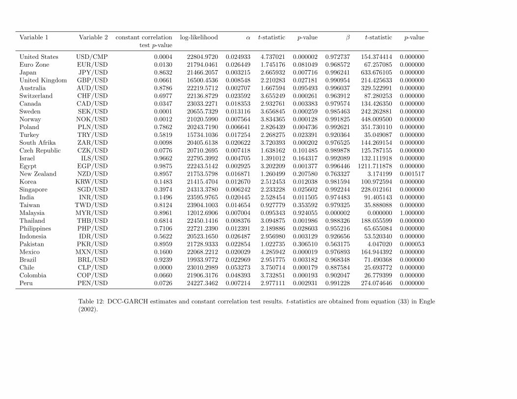
Variable 1 Variable 2 constant correlation log-likelihood α t-statistic p-value β t-statistic p-valuetest p-value

United States USD/CMP 0.0004 22804.9720 0.024933 4.737021 0.000002 0.972737 154.374414 0.000000Euro Zone EUR/USD 0.0130 21794.0461 0.026449 1.745176 0.081049 0.968572 67.257085 0.000000Japan JPY/USD 0.8632 21466.2057 0.003215 2.665932 0.007716 0.996241 633.676105 0.000000United Kingdom GBP/USD 0.0661 16500.4536 0.008548 2.210283 0.027181 0.990954 214.425633 0.000000Australia AUD/USD 0.8786 22219.5712 0.002707 1.667594 0.095493 0.996037 329.522991 0.000000Switzerland CHF/USD 0.6977 22136.8729 0.023592 3.655249 0.000261 0.963912 87.280253 0.000000Canada CAD/USD 0.0347 23033.2271 0.018353 2.932761 0.003383 0.979574 134.426350 0.000000Sweden SEK/USD 0.0001 20655.7329 0.013116 3.656845 0.000259 0.985463 242.262881 0.000000Norway NOK/USD 0.0012 21020.5990 0.007564 3.834365 0.000128 0.991825 448.009500 0.000000Poland PLN/USD 0.7862 20243.7190 0.006641 2.826439 0.004736 0.992621 351.730110 0.000000Turkey TRY/USD 0.5819 15734.1036 0.017254 2.268275 0.023391 0.920364 35.049087 0.000000South Afrika ZAR/USD 0.0098 20405.6138 0.020622 3.720393 0.000202 0.976525 144.269154 0.000000Czeh Republic CZK/USD 0.0776 20710.2695 0.007418 1.638162 0.101485 0.989878 125.787155 0.000000Israel ILS/USD 0.9662 22795.3992 0.004705 1.391012 0.164317 0.992089 132.111918 0.000000Egypt EGP/USD 0.9875 22243.5142 0.002925 3.202209 0.001377 0.996446 1211.711878 0.000000New Zealand NZD/USD 0.8957 21753.5798 0.016871 1.260499 0.207580 0.763327 3.174199 0.001517Korea KRW/USD 0.1483 21415.4704 0.012670 2.512453 0.012038 0.981594 100.972594 0.000000Singapore SGD/USD 0.3974 24313.3780 0.006242 2.233228 0.025602 0.992244 228.012161 0.000000India INR/USD 0.1496 23595.9765 0.020445 2.528454 0.011505 0.974483 91.405143 0.000000Taiwan TWD/USD 0.8124 23904.1003 0.014654 0.927779 0.353592 0.979325 35.888088 0.000000Malaysia MYR/USD 0.8961 12012.6906 0.007004 0.095343 0.924055 0.000002 0.000000 1.000000Thailand THB/USD 0.6814 22450.1416 0.008376 3.094875 0.001986 0.988326 188.055599 0.000000Philippines PHP/USD 0.7106 22721.2390 0.012391 2.189886 0.028603 0.955216 65.655084 0.000000Indonesia IDR/USD 0.5622 20523.1650 0.026487 2.956980 0.003129 0.926656 53.520340 0.000000Pakistan PKR/USD 0.8959 21728.9333 0.022854 1.022735 0.306510 0.563175 4.047020 0.000053Mexico MXN/USD 0.1600 22068.2212 0.020029 4.285942 0.000019 0.976893 164.944392 0.000000Brazil BRL/USD 0.9239 19933.9772 0.022969 2.951775 0.003182 0.968348 71.490368 0.000000Chile CLP/USD 0.0000 23010.2989 0.053273 3.750714 0.000179 0.887584 25.693772 0.000000Colombia COP/USD 0.0660 21906.3176 0.048393 3.732851 0.000193 0.902047 26.779399 0.000000Peru PEN/USD 0.0726 24227.3462 0.007214 2.977111 0.002931 0.991228 274.074646 0.000000

Table 12: DCC-GARCH estimates and constant correlation test results. t-statistics are obtained from equation (33) in Engle(2002).

References

Agmon, T. (1972). The relations among equity markets: a study of share

price co-movements in the United States, United Kingdom, Germany and

Japan. The Journal of Finance 27 (4), 839–855.

Ahn, S. and J. Fessler (2003). Standard errors of mean, variance, and stan-

dard deviation estimators. Technical report, University of Michigan.

Ammer, J., F. Cai, and C. Scotti (2011). Has international financial co-

movement changed? Emerging markets in the 2007–2009 financial crisis.

Contemporary Studies in Economic and Financial Analysis 93, 231–253.

Aydemir, O. and E. Demirhan (2009). The Relationship between Stock Prices

andExchange Rates. Evidence from Turkey. International research Journal

of Finance and Economics 23, 207 – 215.

Balasubramanyan, L. (2004). Do time-varying covariances, volatility comove-

ment and spillover matter? Technical report, Pennsylvania State Univer-

sity.

Baur, D. (2003). What is co-movement? Technical report, European Com-

mission, Joint Research Centre, Institute for the Protection and the Secu-

rity of the Citizen, Technological and Economic Risk Management Unit.

BIS, B. (2010, September). Triennial central bank survey. Foreign exchange

and derivatives market activity in April 2010. Technical report, Bank for

International Settlements.

46

BNM, B. (2005, June). Malaysia adopts a

managed float for the ringgit exchange rate.

http://www.bnm.gov.my/index.php?ch=8&pg=14&ac=1054. Press

release.

Bollerslev, T. (1986). Generalized autoregressive conditional heteroskedas-

ticity. Journal of econometrics 31 (3), 307–327.

Bollerslev, T. (1990). Modelling the coherence in short-run nominal exchange

rates: a multivariate generalized ARCH model. The Review of Economics

and Statistics 72 (3), 498–505.

Brockman, P., I. Liebenberg, and M. Schutte (2010). Comovement, infor-

mation production, and the business cycle. Journal of Financial Eco-

nomics 97, 107–129.

Brooks, R. and M. Del Negro (2004). The rise in comovement across national

stock markets: market integration or IT bubble? Journal of Empirical

Finance 11 (5), 659–680.

Campbell, J. Y., M. Lettau, B. G. Malkiel, and Y. Xu (2001). Have individual

stocks become more volatile? An empirical exploration of idiosyncratic

risk. The Journal of Finance 56 (1), 1–43.

Chair of Financial Engineering and Derivatives (2011). Karlsruhe Institute

of Technology.

Connolly, R., C. Stivers, and L. Sun (2007). Commonality in the time-

variation of stock-stock and stock-bond return comovements. Journal of

Financial Markets 10 (2), 192–218.

47

D’Ecclesia, R. et al. (2006). Comovements and correlations in international

stock markets. European Journal of Finance 12 (6-7), 567–582.

Dimitrova, D. (2005). The Relationship between Exchange Rates and Stock

Prices: Studied in a Multivariate Model. Issues in Political Economy 14.

Engle, R. (1982). Autoregressive conditional heteroscedasticity with esti-

mates of the variance of United Kingdom inflation. Econometrica: Journal

of the Econometric Society 50 (4), 987–1007.

Engle, R. (2002). Dynamic conditional correlation. Journal of Business and

Economic Statistics 20 (3), 339–350.

Engle III, R. and K. Sheppard (2001). Theoretical and empirical properties

of dynamic conditional correlation multivariate GARCH. Technical report,

National Bureau of Economic Research Cambridge, Mass., USA.

Galati, G. and M. Melvin (2004, December). Why has FX trading surged?

Explaining the 2004 triennial survey. BIS Quarterly Review .

Geweke, J. (1982). Measurement of linear dependence and feedback be-

tween multiple time series. Journal of the American Statistical Associa-

tion 77 (378), 304–313.

Gormez, Y. and G. Yilmaz (2007, April). The evolution of exchange rate

regime choices in Turkey. Technical report, Central Bank of the Republic

of Turkey.

Granger, C. (1969). Investigating causal relations by econometric models

48

and cross-spectral methods. Econometrica: Journal of the Econometric

Society 37 (3), 424–438.

Granger, C. W. J., B.-N. Huang, and C.-W. Yang (2000). A bivariate causal-

ity between stock prices and exchange rates: evidence from recent asian

flu. The Quarterly Review of Economics and Finance 40, 337 – 354.

Hashimoto, Y. and T. Ito (2004). High-Frequency Contagion Between the

Exchange Rates and Stock Prices. Working Paper, NBER.

Hatemi-J, A. and M. Irandoust (2002). On the Causality Between Exchange

Rates and Stock Prices: a Note. Bulletin of Economic Research 54 (2),

197–203.

Hochstotter, M., R. Riordan, and A. Storkenmaier (2010). International

Stock Market Comovement and News. Technical report, School of Eco-

nomics and Business Engineering, Karlsruhe Institute of Technology.

IMF, I. (2004, March). Classification of exchange rate arrangements and

monetary policy frameworks. http://www.imf.org/external/np/mfd/er/-

2003/eng/0603.htm.

IMF, I. (2009, February). De facto classification of exchange rate regimes

and monetary policy frameworks. http://www.imf.org/external/np/mfd/-

er/2008/eng/0408.htm.

Jang, H. and W. Sul (2002). The Asian financial crisis and the co-movement

of Asian stock markets. Journal of Asian Economics 13 (1), 94–104.

49

Jobst, A. (2006). Correlation, price discovery and co-movement of asset-

backed securities and equity. Derivatives Use, Trading Regulation 12 (1),

60–101.

Johnson, R. and L. Soenen (2009). European economic integration and stock

market co-movement with Germany. Multinational Business Review 17 (3),

205–228.

Karolyi, G. and R. Stulz (1996). Why do markets move together? An in-

vestigation of US-Japan stock return comovements. The Journal of Fi-

nance 51 (3), 951–986.

Lee, S. and K. Kim (1993). Does the October 1987 crash strengthen the

co-movements among national stock markets. Review of Financial Eco-

nomics 3 (1), 89–102.

Markowitz, H. M. (1952). Portfolio selection. Journal of Finance 7 (1), 77–91.

Meirelles, H. (2009, February). Ten years of floating exchange rates in Brazil.

http://www.bis.org/review/r090129d.pdf. Speech.

MNB, M. (2008). Annual Report 2008. Technical report, Magyar Nemzeti

Bank.

Morana, C. and A. Beltratti (2008). Comovements in international stock

markets. Journal of International Financial Markets, Institutions and

Money 18 (1), 31–45.

Panton, D., V. Lessig, and O. Joy (1976). Comovement of international

50

equity markets: a taxonomic approach. Journal of Financial and Quanti-

tative Analysis 11 (03), 415–432.

Ross, S. (1976). The arbitrage theory of asset pricing. Journal of Economic

Theory 13 (1), 341–360.

Schwarz, G. (1978). Estimating the dimension of a model. The annals of

statistics 6 (2), 461–464.

Sharpe, W. (1964). Capital asset prices: A theory of market equilibrium

under conditions of risk. The Journal of Finance 19 (3), 425–442.

Shiller, R. (1989). Comovements in stock prices and comovements in div-

idends. Technical report, National Bureau of Economic Research Cam-

bridge, Mass., USA.

Shiller, R. and A. Beltratti (1992). Stock prices and bond yields: Can their

comovements be explained in terms of present value models? Journal of

Monetary Economics 30 (1), 25–46.

Thornton, D. and D. Batten (1984). Lag length selection and granger causal-

ity. Technical report, Federal Reserve Bank of St. Louis.

Veldkamp, L. L. (2006). Information markets and the comovement of asset

prices. Review of Economic Studies 73, 823–845.

Wen-Chung, G. and S. Hsiu-Ting (2008). The co-movement of stock prices,

herd behaviour and high-tech mania. Applied Financial Economics 18 (16),

1343–1350.

51