torstein ingebrigtsen bø scenario- and ... - ntnuopen.ntnu.no
TRANSCRIPT
Doctoral theses at NTNU, 2016:47
Doctoral theses at NTN
U, 2016:47
Torstein Ingebrigtsen Bø
Torstein Ingebrigtsen Bø
Scenario- and Optimization-BasedControl of Marine Electric PowerSystems
ISBN 978-82-326-1434-9 (printed version)ISBN 978-82-326-1435-6 (electronic version)
ISSN 1503-8181
NTNU
Nor
weg
ian
Univ
ersi
ty o
fSc
ienc
e an
d Te
chno
logy
Facu
lty o
f Inf
orm
atio
n Te
chno
logy
,M
athe
mat
ics
and
Elec
tric
al E
ngin
eerin
gDe
part
men
t of E
ngin
eerin
g Cy
bern
etic
s
Norwegian University of Science and Technology
Thesis for the degree of Philosophiae Doctor
Torstein Ingebrigtsen Bø
Scenario- and Optimization-BasedControl of Marine Electric PowerSystems
Trondheim, March 2016
Faculty of Information Technology,Mathematics and Electrical EngineeringDepartment of Engineering Cybernetics

NTNUNorwegian University of Science and Technology
Thesis for the degree of Philosophiae Doctor
ISBN 978-82-326-1434-9 (printed version)ISBN 978-82-326-1435-6 (electronic version)ISSN 1503-8181
Doctoral theses at NTNU, 2016:47
© Torstein Ingebrigtsen Bø
Faculty of Information Technology,Mathematics and Electrical EngineeringDepartment of Engineering Cybernetics
Printed by Skipnes Kommunikasjon as
Summary
Diesel electric propulsion has become the industry standard for e.g., oil andgass vessels, cruise vessels, ferries, and vessels with dynamic positioning(DP) systems. Diesel engines are paired with generators to produce electricenergy, which is used by electric motors for propulsion of the vessel, and alsoby other consumers, such as hotel loads, drilling drives, cranes, and heavecompensators. This system is reliable and efficient due to the flexibility ofthe electric grid. DP is often used as a motivating example in this thesis.The thrusters of a vessel using DP is used to fix the position and heading ofthe vessel. The power plant is operated with redundancy, as a single faultshould not lead to loss of position. However, this redundancy decreases theefficiency of the power plant. This thesis presents new ideas and results onhow to increase the efficiency of a hybrid power plant with diesel generatorsets and batteries while maintaining the required safety level.
A model of a marine vessel is presented in Chapter 2. This model in-cludes the power plant, a hydrodynamic model, and control systems. Thepower plant includes generator sets, batteries, switchboards, thrusters, andhotel loads. Environmental loads are included in the hydrodynamic model,such as first and second order wave loads, mean and gusting wind, andocean current, along with the hydrodynamic model of the vessel and thethrusters. The included control systems are a power management system, aDP-controller, thrust allocation, and low level controllers of producers andconsumers. Earlier marine vessel simulators mainly focused on the hydrody-namic model or the power plant. However, the present model combines thethree models, to investigate the complex integration and interaction effectsbetween the models. These interaction effects are especially important wheninvestigating the DP performance after faults in the power plant. Chapter 2presents the models needed for this integration. Three simulation cases arepresented, to shows that the simulator can capture the interaction effects.
A simulation-based dynamic consequence analysis is presented in Chap-
iii
iv
ter 3. The tool uses the simulator from Chapter 2 to simulate several possi-ble worst case scenarios. This tool can be used by the operator to optimizethe electric power plant configuration, and to show that no single failurelead to loss of position. The dynamic consequence analysis is necessarywhen stand-by generators are considered, as the vessel may lose positionduring the time from when the fault occurs until the plant fully recovers,even if the vessel maintains its position after recover.
A scenario-based model predictive controller (MPC) is presented inChapter 4. This controller uses fault scenarios, internally, to constrain thenominal trajectory, which is an alternative to conventional static safety con-straints. The control of generator set speed of a marine power plant is usedas a case study. Simulations show that fault scenarios can replace staticsafety constraints by using this controller.
Chapter 5 presents a method to control peak-shaving. Peak-shaving bybatteries is used to cancel out power fluctuations, which cause variationsin the electric grid’s frequency. However, the batteries may get too hotif power demand is too large. The proposed controller, based on a powerspectrum analysis and MPC, reduces the power fluctuations as much aspossible without letting the battery get too hot. Simulations using datagenerated by the simulator in Chapter 2 showed that the controller canachieve these objectives as long as the characteristics of the load does notchange too rapidly.
Use of the vessel itself as energy storage during DP operation is ex-plored in Chapter 6. A vessel oscillates about its mean position by reducingthe thruster power when the total power demand of the vessel is high andincreasing it during periods of low power consumption. An analytical for-mula for motion amplitude given by power amplitude is calculated in thischapter. The formula is compared with simulations, and the simulation re-sults agreed with the formula. It is also shown that the resulting deviationsin position from variations of several megawatts are no larger than typicalposition deviations from the dynamics of ocean waves and wind.
The proposed models and controllers are demonstrated through simula-tions using MATLAB/SIMULINK. The MPC-based controllers are imple-mented in ACADO.
Acknowledgments
This thesis is the main result of my doctoral studies, undertaken in theperiod August 2012 through December 2015 at the Norwegian Universityof Science and Technology (NTNU). Funding was provided by the Re-search Council of Norway, Kongsberg Maritime, and DNV-GL, through theproject entitled “Design to verification of control systems for safe and en-ergy efficient vessels with hybrid power plants” (D2V, NFR: 210670/070,223254/F50), which is an affiliated project of Center of Autonomous Ma-rine Operations and Systems (AMOS).
This thesis has been supervised by Professor Tor Arne Johansen at Cen-ter of Autonomous Marine Operations and Systems, Department of Engi-neering Cybernetics; Professor Asgeir J. Sørensen at Center of AutonomousMarine Operations and Systems, Department of Marine Technology; andProfessor Roger Skjetne at Department of Marine Technology. I wouldmost of all like to thank my supervisor, Professor Tor Arne Johansen, forguiding me through the PhD. He has introduced me to the world of modelpredictive control, helped me arrange my visit to the University of Newcas-tle, Australia, and continuously supported me. I would also like to thankmy co-supervisors, Professor Asgeir Sørensen and Roger Skjetne, for givingme insight into their knowledge of diesel electric propulsion and dynamicpositioning, but also for their valuable feedback and support. Thanks go toKongsberg Maritime and DNV GL for their financial support and knowl-edge of industry. Special thanks goes to Eirik Mathiesen at KongsbergMaritime. It has been very motivating to have such an enthusiastic andsupportive partner, who shares the challenges of the industry with us.
I would also like to thank my colleagues, including Associate ProfessorEilif Pedersen, Professor Ingrid Utne, PhD Alexander Veksler, and PhDstudents D. K. M. Kufoalor (Giorgio), Espen Skjong, Kevin Koosup Yum,Andreas Reason Dahl, Michel Rejani Miyazaki, Laxminarayan Thorat, andBørge Rokseth. They have all contributed with valuable input and dis-
v
vi
cussions. I would like to give thanks to all of my fellow colleges at De-partment for Engineering Cybernetics, Department for Marine Technology,and AMOS for a good working and social environments in and outside theuniversity.
I would like to express my gratitude to my climbing buddies, who havepatiently listened, and giving me betas for climbs, life, and the PhD. I wouldalso like to thank my friends and family for their support. Finally, I wouldlike to give special thanks to my parents, Karl Ove Ingebrigtsen and AudhildBø, for always being there for me and supporting my choices.
Trondheim, December 2015 Torstein Ingebrigtsen Bø
Contents
Summary iii
Acknowledgments v
Abbreviations xi
1 Introduction 11.1 Background . . . . . . . . . . . . . . . . . . . . . . . . . . . . 1
1.1.1 Dynamic Positioning . . . . . . . . . . . . . . . . . . . 31.1.2 Diesel Electric Propulsion . . . . . . . . . . . . . . . . 31.1.3 Marine Automation . . . . . . . . . . . . . . . . . . . 61.1.4 Model Predictive Control . . . . . . . . . . . . . . . . 10
1.2 Current Trends . . . . . . . . . . . . . . . . . . . . . . . . . . 111.3 Motivation . . . . . . . . . . . . . . . . . . . . . . . . . . . . 151.4 Publications . . . . . . . . . . . . . . . . . . . . . . . . . . . . 171.5 Structure of the Thesis and Main Contributions . . . . . . . . 18
2 Marine Vessel and Power Plant System Simulator 212.1 Introduction . . . . . . . . . . . . . . . . . . . . . . . . . . . . 21
2.1.1 Shipboard Electrical System . . . . . . . . . . . . . . . 212.1.2 Previous Work . . . . . . . . . . . . . . . . . . . . . . 222.1.3 Design of System Simulators . . . . . . . . . . . . . . 232.1.4 Use Cases . . . . . . . . . . . . . . . . . . . . . . . . . 252.1.5 Contribution . . . . . . . . . . . . . . . . . . . . . . . 262.1.6 Overview of the Chapter . . . . . . . . . . . . . . . . . 26
2.2 Modeling . . . . . . . . . . . . . . . . . . . . . . . . . . . . . 262.2.1 Simulator Overview . . . . . . . . . . . . . . . . . . . 262.2.2 Power Management System . . . . . . . . . . . . . . . 302.2.3 Bus Voltage Calculation . . . . . . . . . . . . . . . . . 30
vii
viii Contents
2.2.4 Generator . . . . . . . . . . . . . . . . . . . . . . . . . 322.2.5 Diesel Engine . . . . . . . . . . . . . . . . . . . . . . . 332.2.6 Energy Storage Devices . . . . . . . . . . . . . . . . . 382.2.7 Thrusters . . . . . . . . . . . . . . . . . . . . . . . . . 392.2.8 Other Components . . . . . . . . . . . . . . . . . . . . 412.2.9 Vessel, Environment, Observer, and DP Controller . . 41
2.3 Verification . . . . . . . . . . . . . . . . . . . . . . . . . . . . 412.3.1 Electric Model . . . . . . . . . . . . . . . . . . . . . . 422.3.2 Diesel Engine Model . . . . . . . . . . . . . . . . . . . 422.3.3 Rate Constrained Diesel Engine Model . . . . . . . . . 45
2.4 Case Study . . . . . . . . . . . . . . . . . . . . . . . . . . . . 452.4.1 DP Operation Scenario . . . . . . . . . . . . . . . . . 472.4.2 Bus Opening Scenario . . . . . . . . . . . . . . . . . . 492.4.3 Energy Storage Devices . . . . . . . . . . . . . . . . . 49
2.5 Conclusion . . . . . . . . . . . . . . . . . . . . . . . . . . . . 52
3 Dynamic Consequence Analysis of Marine Electric PowerPlant in Dynamic Positioning 533.1 Method Overview . . . . . . . . . . . . . . . . . . . . . . . . . 56
3.1.1 Method Overview . . . . . . . . . . . . . . . . . . . . 563.1.2 Simulator . . . . . . . . . . . . . . . . . . . . . . . . . 573.1.3 Fault Modeling . . . . . . . . . . . . . . . . . . . . . . 593.1.4 Acceptance Evaluation . . . . . . . . . . . . . . . . . . 603.1.5 Environment Modeling . . . . . . . . . . . . . . . . . . 60
3.2 Simulation Study . . . . . . . . . . . . . . . . . . . . . . . . . 613.2.1 Case Plant . . . . . . . . . . . . . . . . . . . . . . . . 613.2.2 Simulation Results . . . . . . . . . . . . . . . . . . . . 643.2.3 Discussion . . . . . . . . . . . . . . . . . . . . . . . . . 72
3.3 Conclusion . . . . . . . . . . . . . . . . . . . . . . . . . . . . 75
4 Dynamic Safety Constraints by Scenario-Based EconomicModel Predictive Control 774.1 Introduction . . . . . . . . . . . . . . . . . . . . . . . . . . . . 774.2 Problem Statement . . . . . . . . . . . . . . . . . . . . . . . . 794.3 Model Description . . . . . . . . . . . . . . . . . . . . . . . . 804.4 Fault-Tolerant MPC . . . . . . . . . . . . . . . . . . . . . . . 81
4.4.1 Predicted Trajectories . . . . . . . . . . . . . . . . . . 814.4.2 State Constraints . . . . . . . . . . . . . . . . . . . . . 834.4.3 Robust Control Input . . . . . . . . . . . . . . . . . . 844.4.4 Terminal Constraints . . . . . . . . . . . . . . . . . . . 84
Contents ix
4.4.5 Optimization Problem . . . . . . . . . . . . . . . . . . 864.5 Feasibility and Stability . . . . . . . . . . . . . . . . . . . . . 884.6 Reconfigurable Control . . . . . . . . . . . . . . . . . . . . . . 904.7 Case Study . . . . . . . . . . . . . . . . . . . . . . . . . . . . 92
4.7.1 Linear Plant with Nonlinear Cost . . . . . . . . . . . . 924.7.2 Marine Electric Power Plant . . . . . . . . . . . . . . 95
4.8 Conclusion . . . . . . . . . . . . . . . . . . . . . . . . . . . . 100
5 Battery Peak-Shaving Control in Electric Marine PowerPlant using Nonlinear Model Predictive Control 1015.1 Introduction . . . . . . . . . . . . . . . . . . . . . . . . . . . . 1015.2 Control Plant . . . . . . . . . . . . . . . . . . . . . . . . . . . 1045.3 Chance Constraint . . . . . . . . . . . . . . . . . . . . . . . . 1075.4 Model Predictive Control . . . . . . . . . . . . . . . . . . . . 1095.5 Simulation Study . . . . . . . . . . . . . . . . . . . . . . . . . 1105.6 Conclusion . . . . . . . . . . . . . . . . . . . . . . . . . . . . 1175.7 Appendix: Mathematical Preliminaries . . . . . . . . . . . . . 117
6 Dynamic Positioning System as Dynamic Energy Storageon Diesel-Electric Ships 1196.1 Introduction . . . . . . . . . . . . . . . . . . . . . . . . . . . . 1196.2 A Conceptual Control Architecture for Dynamic Energy Stor-
age in Dynamic Positioning . . . . . . . . . . . . . . . . . . . 1216.3 Dynamic Energy Storage Capacity Analysis . . . . . . . . . . 1246.4 Verification – Case Study . . . . . . . . . . . . . . . . . . . . 1266.5 DP Decision Support and Dynamic Consequence Analysis . . 1296.6 Conclusions . . . . . . . . . . . . . . . . . . . . . . . . . . . . 131
7 Concluding Remarks 1337.1 Conclusion . . . . . . . . . . . . . . . . . . . . . . . . . . . . 1337.2 Further Work . . . . . . . . . . . . . . . . . . . . . . . . . . . 135
Bibliography 137

x Contents
Abbreviations
BESS Battery Energy Storage SystemCO2 Carbon dioxideDP Dynamic PositioningFLR Fast Load ReductionMPC Model Predictive ControlMVM Mean Value ModelPMS Power Management SystemTA Thrust Allocation
xi

xii Contents
Chapter 1
Introduction
1.1 Background
The main motivation for this thesis is to reduce the environmental foot-print of vessels with diesel electric propulsion. Global climate change maybe one of the most important and challenging environmental problems oftoday (Pachauri et al.; 2014). It is estimated that total CO2 emissions fromthe maritime sector in 2012 was 800 million tons (Marine Environment Pro-tection Committee, IMO; 2014). No statistics are available on the emissionsof diesel electric vessels, but the combined CO2 emission of roll-on/roll-offvessels, ferries, and cruise vessels were 117 million tons in 2012. Therefore,reducing emissions from these vessels would be significant for the global en-vironment. Reducing CO2 emitted from marine vessels can be achieved byreducing the fuel consumption, which in addition lowers vessel operationalcost. This is a good incentive for the vessel owner and renters to implementmethods that reduce emissions.
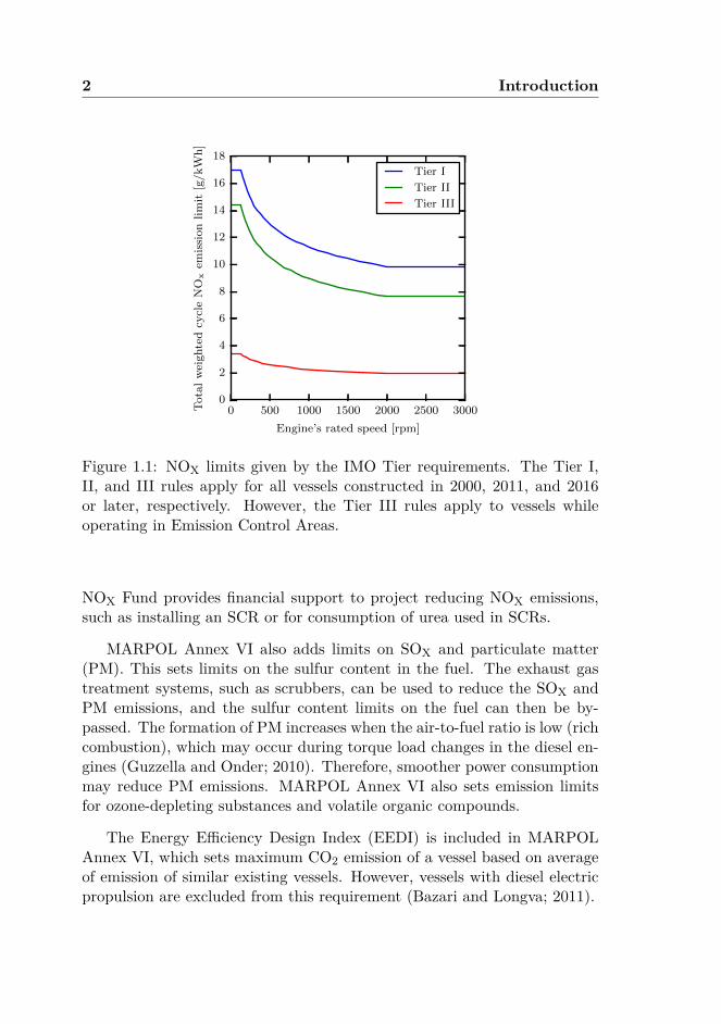
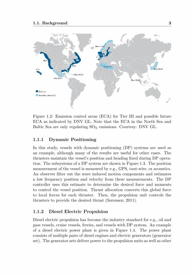
The International Maritime Organization (IMO) sets limits on NOXemissions through MARPOL Annex VI (Figure 1.1) (IMO; 2011). TheTier III requirements are now enforced within the emission control areas onall new vessels in operation and Tier II applies to all new vessels outside ofthese areas (Figure 1.2). Reducing NOX can be achieved by better controlof diesel engines; including new air paths, such as exhaust gas recirculation;or by adding exhaust gas treatment systems, such as selective catalyticreduction (SCR). As NOX form at high temperatures, NOX emissions oftenincrease with a higher engine load. In contrast, SCR requires a minimumtemperature to work and therefore, requires a medium or high engine load.For vessels operating between Norwegian harbors, the Business Sector’s
1
2 Introduction
0 500 1000 1500 2000 2500 3000
Engine’s rated speed [rpm]
0
2
4
6
8
10
12
14
16
18
Tota
lw
eighte
dcy
cle
NO
xem
issi
on
lim
it[g
/kW
h]
Tier I
Tier II
Tier III
Figure 1.1: NOX limits given by the IMO Tier requirements. The Tier I,II, and III rules apply for all vessels constructed in 2000, 2011, and 2016or later, respectively. However, the Tier III rules apply to vessels whileoperating in Emission Control Areas.
NOX Fund provides financial support to project reducing NOX emissions,such as installing an SCR or for consumption of urea used in SCRs.
MARPOL Annex VI also adds limits on SOX and particulate matter(PM). This sets limits on the sulfur content in the fuel. The exhaust gastreatment systems, such as scrubbers, can be used to reduce the SOX andPM emissions, and the sulfur content limits on the fuel can then be by-passed. The formation of PM increases when the air-to-fuel ratio is low (richcombustion), which may occur during torque load changes in the diesel en-gines (Guzzella and Onder; 2010). Therefore, smoother power consumptionmay reduce PM emissions. MARPOL Annex VI also sets emission limitsfor ozone-depleting substances and volatile organic compounds.
The Energy Efficiency Design Index (EEDI) is included in MARPOLAnnex VI, which sets maximum CO2 emission of a vessel based on averageof emission of similar existing vessels. However, vessels with diesel electricpropulsion are excluded from this requirement (Bazari and Longva; 2011).
1.1. Background 3
Figure 1.2: Emission control areas (ECA) for Tier III and possible futureECA as indicated by DNV GL. Note that the ECA in the North Sea andBaltic Sea are only regulating SOX emissions. Courtesy: DNV GL.
1.1.1 Dynamic Positioning
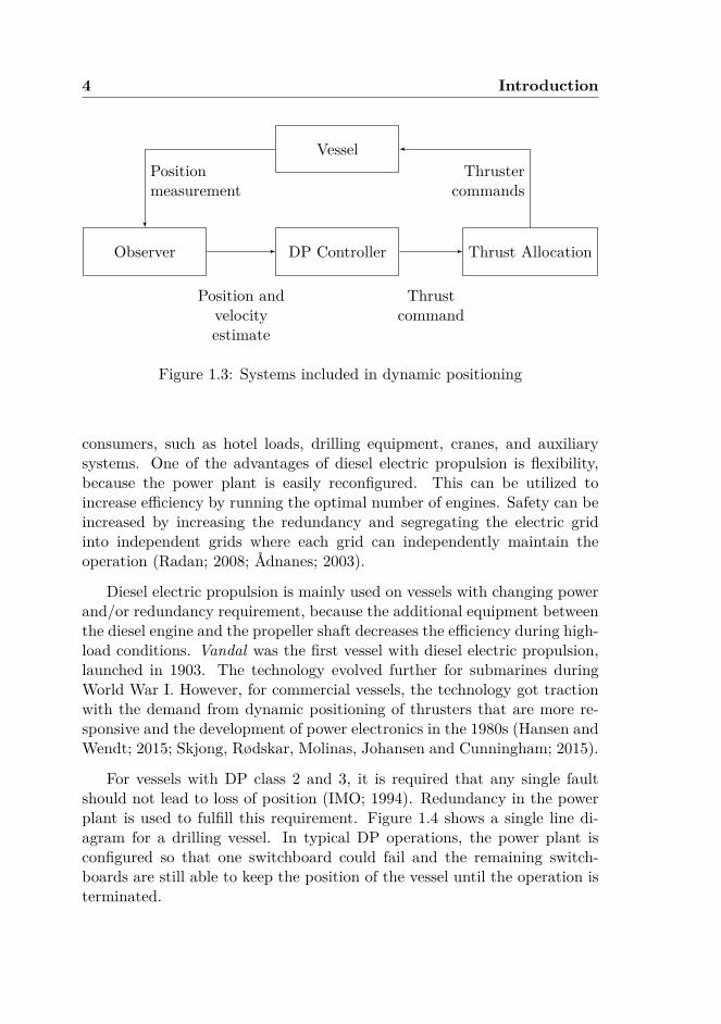
In this study, vessels with dynamic positioning (DP) systems are used asan example, although many of the results are useful for other cases. Thethrusters maintain the vessel’s position and heading fixed during DP opera-tion. The subsystems of a DP system are shown in Figure 1.3. The positionmeasurement of the vessel is measured by e.g., GPS, taut-wire, or acoustics.An observer filter out the wave induced motion components and estimatesa low frequency position and velocity from these measurements. The DPcontroller uses this estimate to determine the desired force and momentsto control the vessel position. Thrust allocation converts this global forceto local forces for each thruster. Then, the propulsion unit controls thethrusters to provide the desired thrust (Sørensen; 2011).
1.1.2 Diesel Electric Propulsion
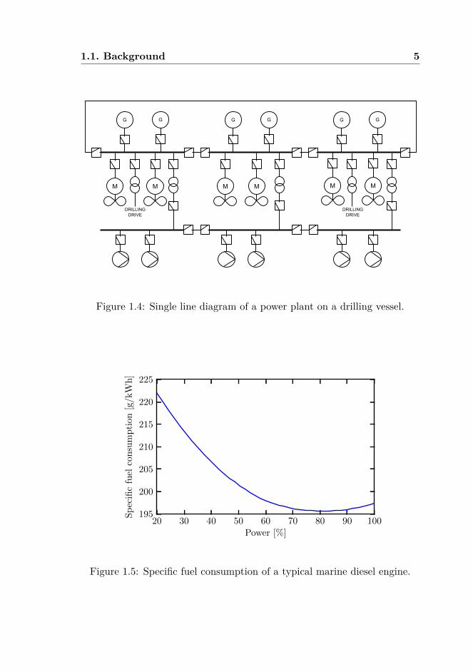
Diesel electric propulsion has become the industry standard for e.g., oil andgass vessels, cruise vessels, ferries, and vessels with DP system. An exampleof a diesel electric power plant is given in Figure 1.4. The power plantconsists of multiple pairs of diesel engines and electric generators (generatorset). The generator sets deliver power to the propulsion units as well as other
4 Introduction
DP ControllerObserver Thrust Allocation
VesselThruster
commands
Thrustcommand
Position andvelocityestimate
Positionmeasurement
Figure 1.3: Systems included in dynamic positioning
consumers, such as hotel loads, drilling equipment, cranes, and auxiliarysystems. One of the advantages of diesel electric propulsion is flexibility,because the power plant is easily reconfigured. This can be utilized toincrease efficiency by running the optimal number of engines. Safety can beincreased by increasing the redundancy and segregating the electric gridinto independent grids where each grid can independently maintain theoperation (Radan; 2008; Ådnanes; 2003).
Diesel electric propulsion is mainly used on vessels with changing powerand/or redundancy requirement, because the additional equipment betweenthe diesel engine and the propeller shaft decreases the efficiency during high-load conditions. Vandal was the first vessel with diesel electric propulsion,launched in 1903. The technology evolved further for submarines duringWorld War I. However, for commercial vessels, the technology got tractionwith the demand from dynamic positioning of thrusters that are more re-sponsive and the development of power electronics in the 1980s (Hansen andWendt; 2015; Skjong, Rødskar, Molinas, Johansen and Cunningham; 2015).
For vessels with DP class 2 and 3, it is required that any single faultshould not lead to loss of position (IMO; 1994). Redundancy in the powerplant is used to fulfill this requirement. Figure 1.4 shows a single line di-agram for a drilling vessel. In typical DP operations, the power plant isconfigured so that one switchboard could fail and the remaining switch-boards are still able to keep the position of the vessel until the operation isterminated.
1.1. Background 5
G
M
G
DRILLING DRIVE
G G G G
DRILLING DRIVE
M M M M M
Figure 1.4: Single line diagram of a power plant on a drilling vessel.
20 30 40 50 60 70 80 90 100
Power [%]
195
200
205
210
215
220
225
Sp
ecifi
cfu
elco
nsu
mp
tion
[g/k
Wh
]
Figure 1.5: Specific fuel consumption of a typical marine diesel engine.
6 Introduction
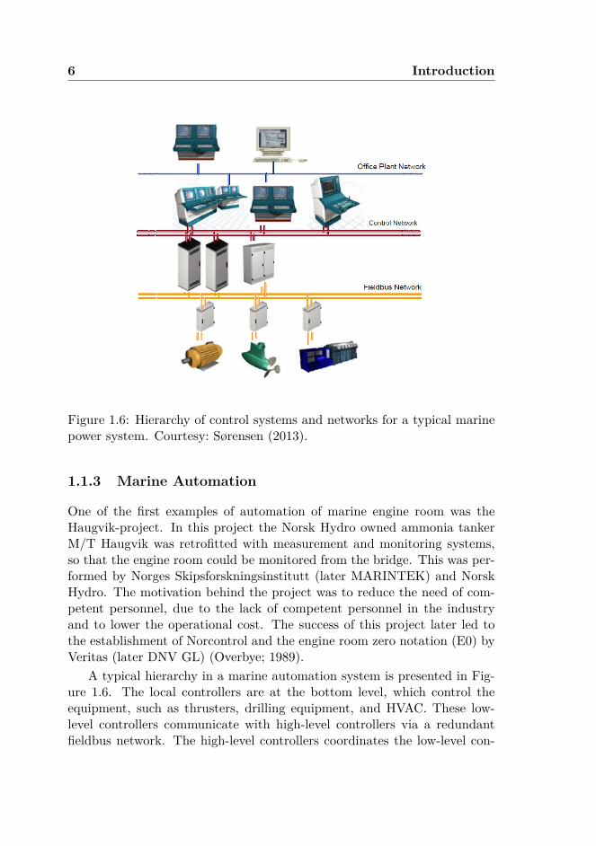
Figure 1.6: Hierarchy of control systems and networks for a typical marinepower system. Courtesy: Sørensen (2013).
1.1.3 Marine Automation
One of the first examples of automation of marine engine room was theHaugvik-project. In this project the Norsk Hydro owned ammonia tankerM/T Haugvik was retrofitted with measurement and monitoring systems,so that the engine room could be monitored from the bridge. This was per-formed by Norges Skipsforskningsinstitutt (later MARINTEK) and NorskHydro. The motivation behind the project was to reduce the need of com-petent personnel, due to the lack of competent personnel in the industryand to lower the operational cost. The success of this project later led tothe establishment of Norcontrol and the engine room zero notation (E0) byVeritas (later DNV GL) (Overbye; 1989).
A typical hierarchy in a marine automation system is presented in Fig-ure 1.6. The local controllers are at the bottom level, which control theequipment, such as thrusters, drilling equipment, and HVAC. These low-level controllers communicate with high-level controllers via a redundantfieldbus network. The high-level controllers coordinates the low-level con-
1.1. Background 7
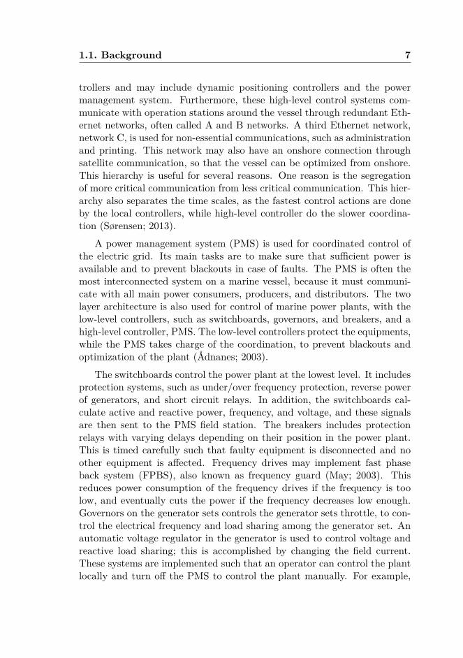
trollers and may include dynamic positioning controllers and the powermanagement system. Furthermore, these high-level control systems com-municate with operation stations around the vessel through redundant Eth-ernet networks, often called A and B networks. A third Ethernet network,network C, is used for non-essential communications, such as administrationand printing. This network may also have an onshore connection throughsatellite communication, so that the vessel can be optimized from onshore.This hierarchy is useful for several reasons. One reason is the segregationof more critical communication from less critical communication. This hier-archy also separates the time scales, as the fastest control actions are doneby the local controllers, while high-level controller do the slower coordina-tion (Sørensen; 2013).
A power management system (PMS) is used for coordinated control ofthe electric grid. Its main tasks are to make sure that sufficient power isavailable and to prevent blackouts in case of faults. The PMS is often themost interconnected system on a marine vessel, because it must communi-cate with all main power consumers, producers, and distributors. The twolayer architecture is also used for control of marine power plants, with thelow-level controllers, such as switchboards, governors, and breakers, and ahigh-level controller, PMS. The low-level controllers protect the equipments,while the PMS takes charge of the coordination, to prevent blackouts andoptimization of the plant (Ådnanes; 2003).
The switchboards control the power plant at the lowest level. It includesprotection systems, such as under/over frequency protection, reverse powerof generators, and short circuit relays. In addition, the switchboards cal-culate active and reactive power, frequency, and voltage, and these signalsare then sent to the PMS field station. The breakers includes protectionrelays with varying delays depending on their position in the power plant.This is timed carefully such that faulty equipment is disconnected and noother equipment is affected. Frequency drives may implement fast phaseback system (FPBS), also known as frequency guard (May; 2003). Thisreduces power consumption of the frequency drives if the frequency is toolow, and eventually cuts the power if the frequency decreases low enough.Governors on the generator sets controls the generator sets throttle, to con-trol the electrical frequency and load sharing among the generator set. Anautomatic voltage regulator in the generator is used to control voltage andreactive load sharing; this is accomplished by changing the field current.These systems are implemented such that an operator can control the plantlocally and turn off the PMS to control the plant manually. For example,
8 Introduction
new generators can be connected by activating the synchronizer, and thegenerator can be manually connected when it is in sync (Ådnanes; 2003).
The PMS is implemented through field stations to control the plantand operating stations for human machine interface. As the loss of a fieldstation should not be the worst case failure on a DP vessel, there is one fieldstation per switchboard or one per generator set. Their physical location ina DP 3 vessel is also important, because they should be segregated in case offire and flooding. The field stations communicate with low-level controllersthrough the field bus network, or directly over hard-wired signals. Hard-wired signals are often used when frequent data updates are needed, suchas to determine breaker status, as an opening of a breaker may requireimmediate coordinated control by the PMS. Two CPUs and a master/slavearchitecture is typical used in field stations, where the slave is ready toimmediately take over control if the master CPU fails (May; 2003).
The operator station is used as the human-machine interface. Multipleoperator stations are placed around the vessel, such as one to monitor thepower plant from the DP control station, and another for control of thepower plant by the engineer. They communicate with the field stationthrough the A and B network.
These are functions typically implemented on a PMS (May and Foss;2000):
Power available: The vessel should have sufficient available power at alltimes. However, sometimes there are not enough power, this may oc-cur due to the connection of large loads or disconnection of producers.The frequency will begin to drop if this situation is not handled cor-rectly, which will give blackout. Thus, a power available signal is used.The available power of the producers is summed and allocated to themain consumers by priority. The reaction time is typically withintenths of a second. In addition, the PMS accepts or rejects connec-tions from large power consumers when required, based on availablepower.
Fast load reduction: FLR is used in addition to power available. TheFLR sets power limitations on the frequency drives of propulsion mo-tors or other motors with frequency drives. These frequency drivesreact within milliseconds due to the fast power electronics. Therefore,FLR is often used for fault events, such as the loss of generator setor opening of bus-tie breakers. The FLR is triggered by hard-wiredsignals and reduces power consumption within tens of milliseconds.
1.1. Background 9
Load shedding: Load shedding is used in extreme cases, when FLR andpower available are insufficient. Consumers are disconnected com-pletely from the grid to reduce power consumption. However, this is adrastic method, because it often takes much effort and time to restartsystems.
Ramp control: Ramps are often used to constrain power increases of con-sumers, so that large load steps on the generators are avoided. Insome cases, these ramps are dynamically set by the PMS dependingon operation and configuration of the vessel.
Automatic start and stop of generator set: Generator sets may be au-tomatically started and connected by the PMS when power demandincreases. This is often performed using start tables. A new generatorset is connected if the power demand increases above a threshold fora certain length of time. Similarly, generators can be disconnectedif the power demand decreases below a threshold for a certain time.Generators are often automatically started and connected in cases ofsevere faults.
Automatic monitoring: The PMS can check health of the system andreact if the system is unhealthy. This is needed as some faults escalatevery quickly. An example is a fault in the governor. If the governorgives full power, the corresponding generator set will take additionalload. The other generator sets may then go into reverse power andtrip. Then, the bus is left with only the unhealthy generator set, andthe future of the plant is uncertain. This may happen within tens ofseconds, which is faster than a human can detect, identify, and reactto the fault. In this case, the PMS should detect and identify the faultand disconnect the generator set before the other generator sets tripon reverse power.
Blackout Recovery: The worst case scenario occurs sometimes, and thepower system blacks out. In such cases, the power system must berecovered carefully. This is often performed by a preprogrammed se-quence, so that the most important equipment is connected first.
Logging: The PMS is also used for logging; the operator uses this optionto optimize the configuration and fault diagnostics.
The PMS is usually operated by the machine room operator who com-municates with the bridge, so that the power plant is correctly configured.
10 Introduction
For example, the bridge may tell the machine room operator that a new op-eration requiring more power will be started soon. Then, the PMS operatormay start and connect additional generator sets and give their acceptancefor the operation to start. The maintenance of diesel engines is typicallyscheduled by the running hour of the engine, which is the number of hoursthe engine has been running. Therefore, the operator select engines forstand-by so that the desired share of running hours is achieved. Althougha load-dependent start is often activated, load-dependent stop is typicallydisabled. The operators often prefer to control this function themselves,so that the engines are not shut down at wrong time and to optimize theindividual share of running hours. However, this can be performed auto-matically, and is often implemented with mode control. The configurationis achieved automatically by selecting the vessel mode (e.g., transit, stand-by, or drilling). The power available is presented for the operator at someoperation station, such as DP and drilling operation station, to indicate thegeneral status of the power plant.
1.1.4 Model Predictive Control
Several methods based on model predictive control (MPC) will be describedin this study. MPC includes a model of the controlled plant. The futuretrajectory of the controlled states is predicted and optimized with respectto a cost function and constraints. This optimization gives an optimalcontrol sequence. The first input in this sequence is applied, at the nextupdate time instant the trajectory and control sequence are optimized, andthe first input of this control sequence is applied. This process is repeatedcontinuously (Maciejowski; 2002).
MPC is in use for DP in Kongsberg Maritimes greenDP system (Kongs-berg Maritime; n.d.). The advertisement for this system claims that thefuel consumption is reduced by approximately 20%, and power fluctuationsare reduced by 50–80%. In this case, the vessel is controlled to move withina region, instead of being controlled to a set point. This approach gives asmoother thrust and small disturbances can be neglected.
MPC has had the largest impact in refining, petrochemical, and otherchemical factories, with more than 2,500 applications in these sectors andin total more than 4,500 applications were collected by Qin and Badgwell(2003). MPC is most attractive for plants with multiple coupled inputsand outputs. The hierarchy typically used to control a plant with MPCsconsist of three levels, a plant controller, high-level MPC controllers, andlow-level controllers. A static plant level optimizer calculates set-points for
1.2. Current Trends 11
the MPC. The MPC is then used for the transition between the set-points,and to keep the plant at the set-points. The MPC provides the set-points forlocal controllers of low-level equipment, such as pumps, valves, and motordrives. It is also common for the plant optimizer to produce a range insteadof set-points for the output variables of the plant, such as in the greenDP.The disadvantage of MPC is the need of a good model of the plant, whichare needed for accurate predictions, and computational complexity, whichchallenges reliable real-time implementations.
MPC has already been proposed for marine power systems and can beused to control power generation, e.g., Hansen et al. (1998); Paran et al.(2015); Veksler et al. (2013). It has also been suggested to use MPC for thecoordinated control of producers and consumers, e.g., Park et al. (2015);Stone et al. (2015); Veksler et al. (2012b). MPC can control active filtersto reduce harmonic distortion, e.g., Skjong, Molinas and Johansen (2015);Skjong, Molinas, Johansen and Volden (2015); Skjong, Ochoa-Gimenez,Molinas and Johansen (2015).
1.2 Current Trends
Many initiatives have been implemented in the last few years to reducemarine power plants emissions, e.g., Hansen et al. (2011); Mathiesen et al.(2012); Myklebust and Ådnanes (n.d.); Veksler et al. (2013). New classifi-cation rules allows startup of stand-by diesel engines and thrusters after afailure e.g., DNV (2015, Part 6 Chapter 26 Section 2) and ABS (2014, Sec-tion 8), and to operate with closed bus-ties; however, this challenges redun-dancy (DNV GL; 2015a). Moreover, the number of diesel engines runningcan be reduced, which will increase efficiency and reduce maintenance.
The combination of diesel electric and diesel mechanic propulsion hasalso been suggested (Myklebust and Ådnanes; n.d.). Methods for reducingload variations have been presented, such as batteries (Kim et al.; 2015),super-capacitors (Chen et al.; 2010), feed-forward control of generators, andload compensation using thrusters (Mathiesen et al.; 2012).
Battery and power electronics have been developed rapidly and severalvendors invests in the development of batteries for marine vessels (ABB;n.d.; Martini; 2015; Valmot; 2014) and DNV GL allow the use of batteriesduring DP operation from January 1, 2016 (DNV GL; 2015b, Part 6 Chap-ter 3). Batteries are being used as the main power supply for a ferry (Mar-tini; 2015). The maritime battery forum (Norwegian forum by DNV GL)reported that 26 vessels are using batteries among their member organiza-
12 Introduction
tions (Opsand; 2015). Some advantages of batteries include:
• Peak-shaving, using the batteries (or super-capacitors) to reduce powerfluctuations. This may reduce wear and tear on the diesel engines,increase efficiency, and batteries make it easier to synchronize newgenerators into the grid.
• Stand-by emergency power/uninterruptible power supply. Today thenumber of diesel engines has been set such that there is sufficientpower available if a fault occurs, which gives a low utilization of thediesel engines. Currently, two generator sets are used in cases whenonly one is required during fault-free operation. Thus, if one generatorfails, the other can maintain power production. However, if batteriesare being used, one generator set can run, and the battery can takethe full load until a new generator set is connected to the grid or theoperation is terminated.
• A battery can be used to run the diesel engines at optimal load. First,the diesel engines can run at the optimal utilization and charge a bat-tery with the excess power. Then, when the battery is fully charged,the diesel engine can be turned off. The battery will then supply theneeded power, until the diesel engine is turned on again when thebattery charge is depleted. This requires many charging/dischargingcycles, which destroys the battery in the end. Therefore, the eco-nomics of this method should be studied to check if the reduction infuel consumption pays off the extra wear and tear on the battery.
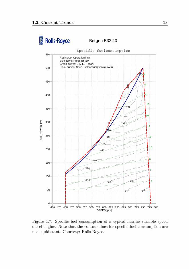
Direct current (DC) distribution should not be ignored when evaluatingthe future of diesel electric propulsion (Hansen andWendt; 2015). DC allowsthe use of variable speed engines, which can increase efficiency. Figure 1.7shows the specific fuel consumption for a variable speed engine. Note thatthe optimal speed of the engine varies with power. Other advantages ofDC include simplified connection of DC power sources, no frequency limitson the generators (or electric grid), and no reactive power. However, somechallenges exist considering high power use cases and short circuits.
Many new combinations of systems (or so-called hybrid concepts,) willsoon be available in which the best of several systems are combined, such asdiesel electric and batteries, AC and DC, and diesel-electric and mechanic.Even more complex systems will be developed than those available today.The needs for better verification (e.g., HIL (Johansen and Sørensen; 2009)),decision support, and autonomous control systems will increase.
1.2. Current Trends 13
400 425 450 475 500 525 550 575 600 625 650 675 700 725 750 775 800SPEED[rpm]
CY
L_P
OW
ER
[kW
]
0
50
100
150
200
250
300
350
400
450
500
550
180
181
182
183
183
184
186
188
190
192
196
200
210220 230
240 250
4
6
8
10
12
14
16
18
20
22
24
Specific fuelconsumption
Bergen B32:40
Red curve: Operation limitBlue curve: Propeller lawGreen curves: B.M.E.P. (bar)Black curves: Spec. fuelconsumption (g/kWh)
Figure 1.7: Specific fuel consumption of a typical marine variable speeddiesel engine. Note that the contour lines for specific fuel consumption arenot equidistant. Courtesy: Rolls-Royce.
14 Introduction
Use of energy storage to optimize a power system was commercializedby the automotive industry in 1996 with the Toyota Prius (Ehsani et al.;2009). A marine power plant has many similar challenges as a hybrid electricvehicle (HEV).
• Power demand varies, in the short-term, e.g., urban driving or loadfluctuations from thrusters in harsh weather, and in the long-term, inslow traffic vs. highway or stand-by operation vs. transit.
• Future perspective of zero-emission zones for cars in cities and formarine vessels in harbor.
• The control of charging and discharging of energy storage is challeng-ing for a hybrid car and a marine vessel, as future power demand ishighly uncertain.
However, more flexibility and higher safety and reliability are required on-board a marine vessel than a HEV. A marine vessel has multiple powerproducers that can be turned on or off. In addition, a marine power plantcontrols its power consumers by constraining their demand; however, thismay be a possible for autonomous cars in the future as well.
There is an increasing trend towards plug-in hybrid electric vehicles(PHEV) (Wirasingha and Emadi; 2011). With the increase of the bat-tery size, the similarities between energy management for marine vehiclesand those for automotive vehicles have become stronger. Different controlstrategies have been suggested to manage energy in a PHEV, including rule-based, fuzzy logic, and optimization-based control (Wirasingha and Emadi;2011).
On-shore power grids are often considered stiff, which means that achange in power for a typically sized consumer or producer in the gridwill result in a small or no change in the voltage and frequency of thegrid. In contrast, marine power grids are considered weak. As consumersand producers can be the same size, a change in the consumed power canresult in large changes in voltage and frequency. However, the increasedrenewable energy penetration in on-shore grids has produced some of thechallenges of marine power plants for onshore power grids. Weisser andGarcia (2005) noted that a wind penetration level of ≥40% is not recordedin autonomous medium-scale power grids, as higher penetration decreasespower quality below the desired level. Holttinen et al. (2011) and Eriksenand Orths (2008) presented some challenges regarding increased penetrationof wind power. These problems typically arise when the level of penetration
1.3. Motivation 15
increases above 10–20%. The reserve requirement increases with increasedwind penetration. The grid is also dependent on the interconnection amonggrids to balance power. This is the case in Denmark, which is dependenton balancing power from neighboring countries. Hydropower plants can beused for energy storage, which is much cheaper than batteries using today’stechnology. Improved wind forecast would improve scheduling, which wouldprovide better predictions of future power production. The domestic gridmust also be reinforced so that geographical imbalances can be handled.Power consumers can also be used to balance power, by controlling electricwater boilers, charging electric vehicles, and cooling houses (Hovgaard et al.;2013). These methods are strongly related to methods suggested for marinepower plants. The interconnection among grids and reinforced grids arerelated to closed bus-tie operations, using hydropower for energy storageis equivalent to using batteries, and better control of consumers is alsoimplemented on marine vessels.
1.3 Motivation
The flexibility of a vessel with DP and diesel electric propulsion gives a largeopportunity to optimize the plant for reduction of environmental emissions.However, the system is highly complex, interconnected, and dynamic, dueto the interactions between the environment and the propulsion, power andcontrol systems. In addition, many operational objectives are conflicting,such as safety requirements and minimization of fuel consumption. As agreater number of diesel engines typically gives a safer vessel, but also in-creased fuel consumption.
Therefore, a large effort was put into the establishment of the systemsimulator. The simulator was needed for the further development and test-ing of new high-level control strategies. A large portion of the time spenton the PhD was used on this development, due to the complexity causedby the number of components, where appropriate models was selected andimplemented to achieve the desired compatibility, fidelity, and computationperformance.
Optimization-based control techniques are ideal for control of these sys-tems. Control objectives can be reformulated to constraints and cost func-tions, and be handled explicitly. One of the constraints is that any singlefault should not lead to loss of position. Scenarios can be used to modelsuch constraints. The vessel can optimize its nominal performance using oneor several predicted scenarios. Then, multiple scenarios modeling multiple
16 Introduction
different faults can be used to ensure the plant’s safety.There are many ways to reduce greenhouse gas emissions from vessels
including:
optimize the operation e.g., better tuning of controllers, new controlstrategies, and coordinated control,
optimize the configuration e.g., turning on or off generator sets, con-necting switchboards,
optimize equipment e.g., proper dimension of needed power ratings, in-creasing the efficiency of thruster drives, and adding
new equipment e.g., batteries, capacitors, active filters, and DC distribu-tion systems.
All of these methods above will be utilized in this thesis, except optimizingthe equipment. The focus is to reduce the number of running generatorsets. Marine diesel engines are typically operated at 20–50% of rated power;however, their optimum is about 80% (Figure 1.5). In addition, some NOXreduction systems do not operate if the exhaust gas is too cold; therefore,a high engine utilization is required to achieve a high enough exhaust gastemperature. There are many reasons to run at low power, including:
Unclear situation: The operator of the vessel must be sure that the vesselis safe. However, the operator may not know the current safety statusof the vessel. A situation in which the vessel is running with an un-necessary high safety level can be avoided by providing more relevantinformation about the vessel’s safety status to the operator. Someoperators override the automatic control system that starts and stopsthe generators because they do not trust or understand the controlsystem.
Frequency variations: The varying electric power demands of a marinevessel may be a reason to increase the number of diesel engines. Al-though the mean power consumption is low, the power variations maycause undesirable large frequency variations. The resulting varyingfrequency makes it difficult to synchronize and connect additional gen-erator sets, and increase the wear and tear on the diesel engines fromthermal and mechanical stress. Consequently, the rotational inertia ofthe plant increases by committing additional generator sets, which re-duces frequency fluctuations. Moreover, the fuel consumption curves
1.4. Publications 17
for diesel engines are given under static load conditions and underes-timate fuel consumption during fluctuating load conditions.
Economy: It is common for some types of vessels for the renter to payfor the fuel of the vessel. Therefore, the vessel owner and operatorof the vessel do not have an incentive to reduce fuel consumption.However, the vessel owner pays for maintenance of the engine, whichoften follows the running hours of the engines. Therefore, mainte-nance is reduced by reducing the number of running engines, whichreduces costs for the vessel owner. However, the cost of interruptingor aborting an operation due to a fault in the power plant is typicallymuch higher than the possible cost reduction by optimizing the plant.Therefore, it may be a large economic risk to reduce redundancy fora more efficient but less robust power plant.
The topics of this thesis are investigating methods for better configura-tions and safer control. Better configurations can be achieved by modeling(Chapter 2), which can be used to design better vessels, and a better decisionsupport system (Chapter 3) so that the operator can make better decisions.The power fluctuations problem can be handled with better control of thegenerator sets (Chapter 4), and use of batteries or thrusters for peak shaving(Chapters 5 and 6). The performance of a given power plant configurationwill increase using these methods (less fuel consumption, less wear and tear,and easier synchronization). In addition, these control methods may makepreviously unsafe configurations safe.
1.4 PublicationsThe following publication are the basis of the thesis:
• Bø, T. I. and Johansen, T. A. (2013). Scenario-based fault-tolerantmodel predictive control for diesel-electric marine power plant, MTS/IEEE Oceans, Bergen, Norway.
• Bø, T. I., Johansen, T. A. and Mathiesen, E. (2013). Unit Commit-ment of Generator Sets During Dynamic Positioning Operation Basedon Consequence Simulation, Proc. 9th IFAC Conf. Control Applica-tions in Marine Systems.
• Bø, T. I. and Johansen, T. A. (2014). Dynamic safety constraints byscenario based economic model predictive control, Proc. IFAC WorldCongress, Cape Town, South Africa, pp. 9412–9418.
18 Introduction
• Bø, T. I., Johansen, T. A., Dahl, A. R., Miyazaki, M. R., Pedersen, E.,Rokseth, B., Skjetne, R., Sørensen, A. J., Thorat, L., Utne, I. B.et al. (2015). Real-time marine vessel and power plant simulation,Proceedings of the ASME 34th International Conference on Ocean,Offshore and Engineering, OMAE 2015.
• Bø, T. I., Johansen, T. A., Sørensen, A. J. and Mathiesen, E. DynamicConsequence Analysis of Marine Electric Power Plant in DynamicPositioning. Submitted for publication
• Bø, T. I. and Johansen, T. A. Dynamic safety constraints by scenario-based economic model predictive control. Submitted for publication.
• Bø, T. I. and Johansen, T. A. Battery Peak-Shaving Control in Elec-tric Marine Power Plant using Nonlinear Model Predictive Control.Submitted for publication.
• Bø, T. I., Dahl, A. R., Johansen, T. A., Mathiesen, E., Miyazaki, M. R.,Pedersen, E., Skjetne, R., Sørensen, A. J., Thorat, L. and Yum, K. K.(2015). Marine vessel and power plant system simulator. Access,IEEE 3: 2065–2079
• Johansen, T. A., Bø, T. I., Mathiesen, E., Veksler, A. and Sørensen,A. J. (2014). Dynamic positioning system as dynamic energy storageon dieselelectric. doi: 10.1109/ACCESS.2015.2496122 ships, PowerSystems, IEEE Transactions on 29(6): 3086–3091.
1.5 Structure of the Thesis and Main Contribu-tions
The thesis is a collection of papers, which makes the chapters self-contained.However, the model used in Chapter 2 was used for the simulations in severalother chapters.
Chapter 2: This chapter presents a marine vessel system simulator. Thesimulator includes marine power, DP, and control systems. The maincontribution is the presentation of the models required for the sys-tem simulator. The motivation behind the simulator was the needfor a simulator that could model the interaction effects between theDP system and the electrical system under nominal conditions andwhen faults occur. More knowledge of the current safety margin can
1.5. Structure of the Thesis and Main Contributions 19
be found by using a simulator which can simulate faults in the electricsystem, how they are handled, and how they affect the stationkeepingperformance. The simulator allows new methods to be tested and ver-ified including interaction effects. In addition, the simulator includesinteraction effects between the DP system and the electric system,such as power fluctuations generated by wave induced motion. Thiscan be used to optimize power producers with load time series fromthe simulator.
Chapter 3: The simulator was used for development of the simulation-based consequence analysis. The main contribution of this chapteris the analysis method. The analysis was performed by establishingall possible worst case scenarios, and simulating them to verify thatthe vessel could maintain its position during the worst case scenario.The method was compared with the conventional static method. Adrilling rig was used in the simulation study with several fault scenar-ios and grid configurations. Different recovery methods were used inthe simulation study to show different transient performance.
Chapter 4: A scenario-based MPC was presented in this chapter. Thecontroller used fault and nominal scenarios internally. The fault sce-narios are used to constrain the nominal scenario, so that the plantcan be maintained within the constraints after a fault scenario occurs.This transfers the safety requirements, given by the fault scenarios,from safety constraints on a nominal trajectory to safety constraintson fault trajectories, which is the main contribution of the chapter. Asit may be difficult to find static constraints for the nominal trajectory,this increases the room for optimization, which may make increase theplant’s performance.The MPC controller is applied on a marine power plant. One of thereasons to use many diesel engines is to provide sufficient rotating iner-tia to withstand a loss of a generator. Lossing a generator increases theload on the remaining generator sets and the frequency will decreasedue to rate constraints on the diesel engine’s torque. This scenariowill lead to a blackout due to under-frequency if the safety margin istoo small or the load is not sufficiently reduced. Therefore, loss of agenerator set was used as the fault scenario in the case study, wherethe set-point of the governor is adjusted by the MPC.The safety margin is dynamic, which allows the electric frequency tovary within a safe range, instead of fixing it to a nominal frequency.
20 Introduction
This may increase the safety margin in some cases, so that the con-figuration is safe in cases where it is unsafe with conventional controlmethods.
Chapter 5: Batteries are useful for peak shaving to reduce load fluctua-tions. The diesel engines will produce a slowly varying load, and thebatteries will handle load fluctuations. Batteries get hot if the electricpower is too high; therefore, power is constrained by the battery tem-perature. This chapter presents a controller that uses a combinationof spectrum and statistical analyses with MPC to control the peakshaving, so that the load fluctuations are canceled by the batteries.However, when the batteries get hot, the most important frequenciesin the load fluctuation are canceled.
Chapter 6: A formula for calculating the position variation given by thepower fluctuation was presented in this chapter. As inertia of a marinevessel is large, kinetic energy is also large, even at low velocities. Largepower fluctuations are canceled out by the thrusters if the vessel isallowed to oscillate around the desired position. The loss is also smallwhen a sufficiently large mean force (e.g., wind or current) is applied tothe vessel. This method allows the vessel to use extra thrust when theelectric power demand is small, and the vessel will then move towardthe mean force. The thrust can be decreased during periods of highpower demand, and the mean force will move the vessel back to itsoriginal position. The mass of the vessel is used as an energy storagedevice to reduce variations in electric power, which is an alternativeto using batteries, flywheels, or a super-capacitor for peak shaving.
Chapter 7: Concluding remarks and future perspectives are presented inthe last chapter.
Chapter 2
Marine Vessel and PowerPlant System Simulator
This chapter is based on Bø et al. (2015).
2.1 Introduction
2.1.1 Shipboard Electrical System
The onboard electric power system is crucial for most modern marine ves-sels conducting advanced operations. Diesel-electric propulsion is commonin offshore oil and gas vessels and cruise/passenger ships with dynamic po-sitioning (DP).
The ability to conduct stationkeeping and maneuvering subject to cur-rent, waves, and wind loads depends on the power plant capacity. Insuffi-cient power may result in decreased DP performance and loss of position.More severely, a total loss of electric power, known as a blackout, results inloss of control of the vessel.
Redundancy in power capacity, distribution, and in the number of gen-erating units is one possible alleviation of the risk of power system faults.However, redundancy is costly. Economical expenses are significant, bothin terms of investment in equipment, which most of the time is not strictlynecessary, and in terms of machine running hours leading to more frequentmaintenance, and increased emissions and fuel consumption.
The mentioned concerns motive the development of new power plantcontrol strategies and the introduction of new power sources. Such stepsare not trivial, due to the complex and strongly interconnected nature of
21
22 Marine Vessel and Power Plant System Simulator
onboard marine power plants, and the weak grid, i.e., sensitive to changesboth in produced and consumed power. Numerical simulation is a valuabletool for investigating such effects at all stages of design, implementation,and operation.
2.1.2 Previous Work
A number of marine power plant simulation solutions exist. The intendeduse ranges from commercial to academic, and the content from a few stateequations to complete software suites. A selection follows:
Marine Cybernetics’ CyberSea technology platform encompasses mod-els of hydrodynamics, electro-mechanics, and sensors (Marine Cyber-netics; n.d.). It is used for independent hardware-in-the-loop (HIL)testing (Johansen and Sørensen; 2009) and dynamic capability analy-sis (DynCap) (Pivano et al.; 2014).
U.S. Office of Naval Research’s Electric Ship Research and Develop-ment Consortium studies include both real-time HIL simulators (Renet al.; 2005), models of higher fidelity (Steurer et al.; 2007), and ex-tension to hybrid plants (Xie et al.; 2009).
Marine Systems Simulator (MSS) (MSS; 2010) library and simulatorfor MATLAB/Simulink is a 2004 merge of (Perez et al.; 2006, Section1): marine GNC toolbox (Fossen; 2002), MCSim (Sørensen et al.;2003), and DCMV (Perez and Blanke; 2003). It has vessel dynamics,environmental (wave, surface current, and wind) loads, and advancedthruster models.
DNV GL’s Sesame Marine DNV GL (n.d.) risk management softwareincludes Marintek’s SImulation of Marine Operations (SIMO) motionand stationkeeping simulator. The system is capable of modelingmultibody systems and flexible systems.
Italian Integrated Power Plant Ship Simulator includes an integratedpower system model implemented in the Simulink environment (Bosichet al.; 2012).
NTNU models include thruster power consumption (Hansen et al.; 2001)and power management system functions (Radan; 2008).

2.1. Introduction 23
NTNU bond graph model library Pedersen and Pedersen (2012) includesa vessel model. The library is also verified through full-scale experi-ments.
Some solutions mainly focus on the electrical system without concernfor the actual DP performance and related consumption, while others dothe opposite.
2.1.3 Design of System Simulators
The simulator presented in this chapter is a system simulator. This meansthat the purpose is to model interactions between each of the subsystems ofthe complete system, and it should be flexible, so that many different casescan be studied. A modular design achieves this.
The use cases of the simulator will determine the dynamics that we needto model and parameterize. The difference in magnitude of the smallest andthe largest timescale of the dynamics in such a multi-physics simulator maybe in order of decades. It is therefore essential to decide the importanttimescales for the particular study.
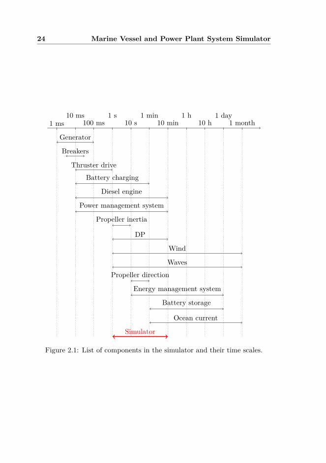
The smallest timescale of the vessel is, in the electric system, in the orderof milliseconds. In the other end, quasistatic studies such as effects of wearand tear, are in the order of months and years. For simulating short-circuit,the fast dynamics must be modeled, while the effects of the environment,and wear and tear, can be assumed constant. On the other hand, theelectric system can be assumed to be in steady state when simulating DPoperation, as the timescales of the electric system are much smaller thanthe timescale of the vessel motion. Figure 2.1 lists the time scale of thesimulator components. For certain components model reductions shouldnot take place, as discussed in respective sections later.
The complexity of a system simulator grows with the number of compo-nents and the fidelity level. By increasing the fidelity level, more parameterswith higher order model structure, and a more thorough verification and val-idation are required. In addition the computational speed will typically bereduced. For studies where high fidelity level is required, not all the sub-models need to be of high fidelity, as long as the model reduction is doneproperly and with care. By using a modular design, it is easy to use lowfidelity models to identify where higher fidelity is required. These modelscan then be replaced with high fidelity models.
Verification and validation is challenging for system simulators due tothe high complexity. Each submodel can be verified by itself, but this
24 Marine Vessel and Power Plant System Simulator
1 ms10 ms
100 ms1 s
10 s1 min
10 min1 h
10 h1 day
1 month
Generator
Breakers
Thruster drive
Battery charging
Diesel engine
Power management system
Propeller inertia
DP
Wind
Waves
Propeller direction
Energy management system
Battery storage
Ocean current
Simulator
Figure 2.1: List of components in the simulator and their time scales.
2.1. Introduction 25
does not verify their integration. Small scale or full scale tests can beused for verification, but this is costly and time consuming. In many casesexperiences from a set of trained operators are the most practical way ofverifying expected system-level performance.
2.1.4 Use Cases
The simulator has been used in several studies considering DP with diesel-electric propulsion and consumers such as hotel loads and motors for drilling,compressors, and pumps.
A selection of typical use cases follows:
Realistic power consumption profile: Since the DP controller and thrus-ter models are interconnected with the power plant, the power loadfluctuations are represented in a realistic way. The interaction be-tween the many control subsystems, such as PMS, thrust allocation,thruster torque, or speed control, is included (Bø and Johansen; 2013).The simulator can therefore be used to generate time series for lateruse in isolated subsystem simulation (e.g., diesel engine simulation).
Fault consequence analysis: The plant behavior in the event of an elec-trical fault, such as the loss of a genset, can be simulated (Bø et al.;2013). The resulting DP performance is then also available. Thismay improve the conventional capability analysis, which is calculatedassuming that the propulsion system is in steady-state. Indeed, tran-sients during plant reconfiguration can be critical (Pivano et al.; 2014).
Operation optimization: The detailed level of modeling includes manystates for each submodule, for instance temperature and power output.Based on these, operation may be optimized with regards to emissions,maintenance, or fuel consumption.
Concept evaluation: Submodules representing new subsystems such asenergy storage device (ESD), can be interfaced to the simulator. Thisallows investigation of new power sources and their effect on the overallcontrol and performance of the plant.
It must be stressed that the simulator is not limited to diesel-electricpropulsion, nor DP operations.
26 Marine Vessel and Power Plant System Simulator
2.1.5 Contribution
This chapter focuses on the models and methods needed for an integratedsimulator of the electric power system together with the vessel motion in-cluding the DP system. Secondly, some new models are established andverified to achieve the desired fidelity level and performance. Most of themodels are verified models from literature. The scope of the simulator runsfrom high-level control systems, such as the positioning system and powermanagement system (PMS), to high-fidelity models of power generators,storage, and consumers, such as gensets, batteries, and thrusters, respec-tively. The accuracy of the simulator is only verified qualitatively due to thecomplexity of the system. Quantitative verification of the plant is researchstill to be done and is considered outside the scope of this chapter.
2.1.6 Overview of the Chapter
This chapter consists of three sections, the model is presented in Section 2.2,the new models are verified in Section 2.3, and simulations are shown inSection 2.4. The modeling section starts with an overview of the simulator,followed by details of the power management system. The electrical com-ponents are then presented, with the switchboard and generator. Next, twomodels of diesel engines are presented, followed by the thruster models. Lastis a presentation of the hydrodynamic model of the vessel, the environmentalforces and the DP control system. In Section 2.3, verification of the electricbus model and simplified diesel-engine model are presented. Section 2.4presents a simulation of a drilling rig in DP operation, then simulation of afault is shown, before a simulation with batteries is presented.
2.2 Modeling
2.2.1 Simulator Overview
The main assumptions of the simulator are:
Steady-state electric system: It is assumed that the electrical system isin steady state, this is done to obtain real-time capabilities. The sim-ulator captures dynamics with time scale down to 1 second. However,the dynamics of the electric system are often in milliseconds and aretherefore assumed to be in steady state, as illustrated in Figure 2.1.This is verified in Section 2.3.1. The simulated electrical variables arefrequency, voltage, active power, and reactive power. It is therefore
2.2. Modeling 27
possible to simulate faults, such as under/over-frequency, slowly de-veloping under/over voltage fault, and reverse power. However, it isnot able to simulate phase imbalance, transient voltage faults, short-circuit, and harmonic distortion.
Mean-value engine model: The diesel engines are modeled by mean-value engine models. This means that most of the components inthe diesel engine system are mathematically modeled based on thephysical laws. However, the in-cylinder process is simplified so thatit gives only a cycle average output such as average shaft torque, andmass and energy flow of the combustion gas.
Power management system: The objective of the PMS is to make surethat the power plant is safe and efficient. More details are given inSection 2.2.2.
Protection relays: Protection relays are not modeled, as breakers can betripped by a timer. This means that some custom protection relaysneed to be implemented to simulate a partial blackout. Alternatively,post-processing can be used to detect when breakers should be opened.
Fixed pitch, variable speed thrusters: The thrusters are assumed tobe fixed pitch propellers, with the possibility to run with variablespeed. Thrusters that can rotate in any direction, azimuth thrusters,and fixed direction thrusters (e.g., tunnel thrusters) can be simulated.
An object-oriented modeling structure has been used to model the ma-rine power plant. This means that each block in the simulator representsa physical component in the vessel, and further subsystem blocks representinternal physical components of the larger system.
The top level view of the model is illustrated by an example in Fig-ure 2.2. This view represents the information flow for motion control ofthe vessel. A DP controller has been used in the presented case. Alterna-tively, the setpoints of the thrusters can be given manually during transit,maneuvering, or other operations without DP control.
For this case, the view contains:
1. Observer; estimates the position and velocity of the vessel from mea-surements.
2. DP control system; calculates a desired thrust command.
28 Marine Vessel and Power Plant System Simulator
u_c
Current velocity
windForce
Wind
eta
nu
nu_r
nu_c
tau wind
tau
Semi-sub1
nu_r
alpha
u
PowerAllocatedThrusters
Force
Electric system
tau_d
alpha
u
power allocated
Thrust allocation
Centraly
tau_est
eta_hat
deta_hat
State observer
nu
eta
eta_hat
eta_dot_hat
eta_d
tau
DP controllereta_d
Setpoint position
Wave Force
Wave
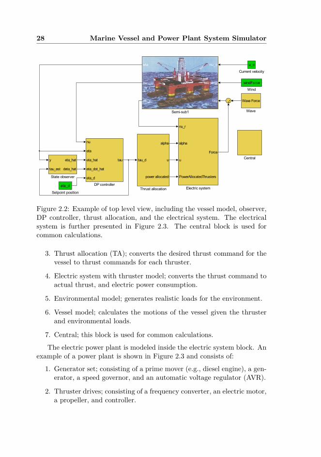
Figure 2.2: Example of top level view, including the vessel model, observer,DP controller, thrust allocation, and the electrical system. The electricalsystem is further presented in Figure 2.3. The central block is used forcommon calculations.
3. Thrust allocation (TA); converts the desired thrust command for thevessel to thrust commands for each thruster.
4. Electric system with thruster model; converts the thrust command toactual thrust, and electric power consumption.
5. Environmental model; generates realistic loads for the environment.
6. Vessel model; calculates the motions of the vessel given the thrusterand environmental loads.
7. Central; this block is used for common calculations.
The electric power plant is modeled inside the electric system block. Anexample of a power plant is shown in Figure 2.3 and consists of:
1. Generator set; consisting of a prime mover (e.g., diesel engine), a gen-erator, a speed governor, and an automatic voltage regulator (AVR).
2. Thruster drives; consisting of a frequency converter, an electric motor,a propeller, and controller.
2.2. Modeling 29
alpha
Gotoalpha
Goto TagVisibility
2alpha
-T-
Goto15
u
Goto18u
Goto TagVisibility6
3u
1nu_r
nu_r
Goto19
nu_r
Goto TagVisibility7
4PowerAllocatedThrusters
powerAllocatedThrusters
Goto TagVisibility1
1Force
Force
Central
swb
Other components 1
swb
Other components 2
swb
Other components 3
Swb1
Brea
ker
Swb2
breaker Swb1
Brea
ker
Swb2
breaker1 Swb1
Brea
ker
Swb2
breaker2
swbI
D
swbI
D
swbI
D
0 1swb
swb
swb
swb
swb
swb
0 10 1
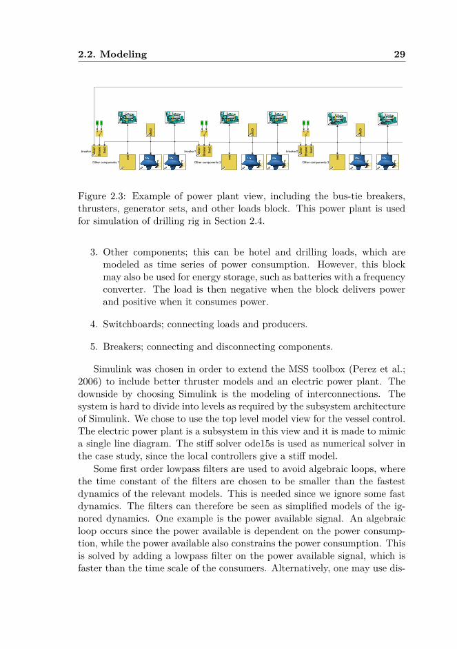
Figure 2.3: Example of power plant view, including the bus-tie breakers,thrusters, generator sets, and other loads block. This power plant is usedfor simulation of drilling rig in Section 2.4.
3. Other components; this can be hotel and drilling loads, which aremodeled as time series of power consumption. However, this blockmay also be used for energy storage, such as batteries with a frequencyconverter. The load is then negative when the block delivers powerand positive when it consumes power.
4. Switchboards; connecting loads and producers.
5. Breakers; connecting and disconnecting components.
Simulink was chosen in order to extend the MSS toolbox (Perez et al.;2006) to include better thruster models and an electric power plant. Thedownside by choosing Simulink is the modeling of interconnections. Thesystem is hard to divide into levels as required by the subsystem architectureof Simulink. We chose to use the top level model view for the vessel control.The electric power plant is a subsystem in this view and it is made to mimica single line diagram. The stiff solver ode15s is used as numerical solver inthe case study, since the local controllers give a stiff model.
Some first order lowpass filters are used to avoid algebraic loops, wherethe time constant of the filters are chosen to be smaller than the fastestdynamics of the relevant models. This is needed since we ignore some fastdynamics. The filters can therefore be seen as simplified models of the ig-nored dynamics. One example is the power available signal. An algebraicloop occurs since the power available is dependent on the power consump-tion, while the power available also constrains the power consumption. Thisis solved by adding a lowpass filter on the power available signal, which isfaster than the time scale of the consumers. Alternatively, one may use dis-
30 Marine Vessel and Power Plant System Simulator
crete time and a delay for these signals, but this reduces the performanceof the chosen implicit ode solver.
2.2.2 Power Management System
The objective of the PMS is to make sure there is always enough poweravailable, to prevent blackout. If a blackout occurs, the power should berestored as fast as possible. The PMS starts additional generators when theexcessive power capacity of the connected producers is too low. In addition,the PMS allocates power to the different consumers, by first summing thecurrent power capacity of the producers, and then sharing this among theconsumers based on their desired power consumption and priority. Thissignal, called power available, is sent to some consumers, stating the max-imum power limit for the specific load. Load shedding (disconnection ofconsumers) is done in extreme cases, when power reduction must be doneimmediately (e.g., close to under-frequency).
Fast load reduction is an alternative method to reduce the power con-sumption quickly. It reduces the load of the thruster drives, since theycan change the power consumption quickly due to the frequency convert-ers. Shortly after the fault is cleared or the capacity is increased, the drivescan increase their loads. This is in contrast to load shedding where theconsumers often needs to be restarted after being disconnected.
The PMS can also adjust the droop and isochronous load sharing pa-rameters to adjust the load sharing. This is done during progressive loadingafter connection of generator sets. Progressive loading is implemented toensure that the power generation of the new producer is slowly increasedfrom no load to desired load sharing.
The PMS algorithm is implemented in C++ as an S-function blockand can easily be configured to different power plants. The object-orientedfocus of the simulator is kept in the PMS implementation, so that newfunctionalities, such as automatic start and stop, can easily be added.
2.2.3 Bus Voltage Calculation
The voltage of the bus is needed to calculate the load sharing of the genera-tors. The generators are connected in parallel as shown in Figure 2.4a. Theloads are assumed to be independent of the bus voltage, their active andreactive power are therefore given. Thévenin equivalent circuit, as shownin Figure 2.4b, of the connected generator sets is used to calculate the bus
2.2. Modeling 31
Ea,n
Zn
Ia,n
Zload
Ea,2
Z2
Ia,2
Ea,1
Z1
Ia,1
−
+
V ...
(a)
ET
ZT
I
Zload
−
+
V
(b)
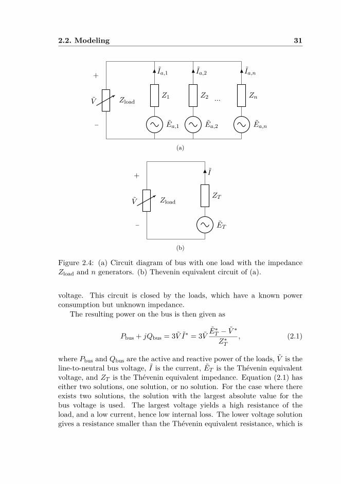
Figure 2.4: (a) Circuit diagram of bus with one load with the impedanceZload and n generators. (b) Thevenin equivalent circuit of (a).
voltage. This circuit is closed by the loads, which have a known powerconsumption but unknown impedance.
The resulting power on the bus is then given as
Pbus + jQbus = 3V I∗ = 3V E∗T − V ∗
Z∗T, (2.1)
where Pbus and Qbus are the active and reactive power of the loads, V is theline-to-neutral bus voltage, I is the current, ET is the Thévenin equivalentvoltage, and ZT is the Thévenin equivalent impedance. Equation (2.1) haseither two solutions, one solution, or no solution. For the case where thereexists two solutions, the solution with the largest absolute value for thebus voltage is used. The largest voltage yields a high resistance of theload, and a low current, hence low internal loss. The lower voltage solutiongives a resistance smaller than the Thévenin equivalent resistance, which is
32 Marine Vessel and Power Plant System Simulator
unphysical. This yields a high current, with very high internal loss sincemost of the voltage drop occurs over the internal impedance.
During simulations it may occur that there exists no valid solution.This may happen when the load increases rapidly (a load is connected) orthe Thévenin equivalent voltage of the generator decreases rapidly (faultin AVR or disconnection of a generator). In such cases, the voltage is setto a low value. This gives an incorrect load sharing, but the AVR willincrease the voltage quickly. During the verification study in Section 2.3.1,a valid solution of the bus voltage was regained within 0.1 millisecond. Thisis permissible since the time is very short compared to the time scale ofthe mechanical system. A lowpass filter must therefore be added whensimulating voltage protection relays.
2.2.4 Generator
In marine power plants, synchronous generators are typically used to pro-duce power. As mentioned earlier, the generator is assumed to be in steadystate and with balanced phases. The electrical torque is
τe = p+ plossω
= p
ω+ r(p2 + q2)
ωv2 , (2.2)
where p and ploss are the active power generated and power loss in thegenerator, r is the resistance in the stator windings, q is the reactive power,and v is the terminal voltage. The terminal line-to-neutral voltage is givenas (Krause et al.; 2013):
Va = −ZIa + Ea, (2.3)
where Z is the internal impedance of the generator set, Ia is the currentthrough phase a and Ea is the induced line-to-neutral voltage for phase a.
It is assumed that the magnitude of Ea is perfectly controlled by theAVR or at least the dynamics are much faster than the dynamics of themechanical system. This is verified in Section 2.3.1. The per phase angle ofEa is
∠Ea = θNpoles2 , (2.4)
where θ is the mechanical angle and Npoles is the number of poles of thegenerator. Parameters are found from (Krause et al.; 2013).
The AVR regulates the terminal voltage by manipulating the inducedvoltage. In this simulator, we use a droop controller to determine the set-point, based on the reactive power of the generator set. This takes care of
2.2. Modeling 33
the reactive load sharing. The generators deliver equal amount of reactivepower if they have equal voltage droop curves.
2.2.5 Diesel Engine
The dynamics of the diesel engine are the slowest dynamics of a diesel elec-tric power plant. Most modern diesel engines are turbocharged to provideincreased power density. When a turbocharged diesel engine needs to in-crease its delivered power, more air is required into the cylinders to avoidincomplete combustion and visible smoke in the exhaust. However, theresponse of the air system is slow, due to the rotating inertia of the tur-bocharger and the large air and exhaust receiver volumes. This gives rise tothe turbo-lag. In addition, increasing the fuel injection rises the temperaturein the cylinder.
Constraints are, therefore, added to the engine control output by theengine manufacturer to ensure that the fuel injection is not changed tooquickly. This is done to avoid that the engine is damaged by a rapid changeof temperature, and that the air pressure in the inlet manifold is largeenough to allow for complete combustion. These constraints are in somecases conservative, and the air dynamics may be neglected since the enginewill always run with complete combustion due to these constraints.
Transients of the diesel engines can be grouped into three categories (Be-najes et al.; 2002). The first is energy transfer delay which happens due tosignal delay, preset valve closure or injection timing. The time scale ofsuch phenomena is in milliseconds. In simulation, this can only be seen bydetailed modeling of the cylinder process and the fuel injection system. Sec-ondly, the already mentioned air dynamics are the most interesting physicsin this kind of application. The typical transient time scale of the air dynam-ics is in seconds. Lastly, the thermal transients are caused by the thermalinertia of the system, which may have time scale of tens of minutes.
Mean Value Model
The main purpose of the diesel engine simulation model is to capture the airdynamics including pressure before the engine cylinder which can be relatedto the charge air available for combustion. In the mean value engine model,most of the physics in the engine system components are captured exceptfor the in-cylinder process, i.e., the thermodynamic cycle. The main com-ponents included in the model are an engine cylinder block, a turbocharger,a charge air cooler, an air receiver, and an exhaust receiver. The imple-
34 Marine Vessel and Power Plant System Simulator
mented mean value engine model is based on the models presented in Chowand Wyszynski (1999); Guzzella and Onder (2010); Heywood (1988); Ped-ersen and Engja (2000); Yum and Pedersen (2013); Zacharias (1967).
The engine system including a turbocharging system is inherently a ther-modynamic process with gas mixture as medium. Therefore, main variablesof the system are pressure, p; temperature, T ; and fuel-air equivalent ra-tio, F . Also flow variables, such as mass flow of gas, m; enthalpy flow orrate of change in internal energy, E; and mass flow of burned fuel, mb, arenecessary to describe the dynamics of the system.
A filling and emptying method (Chow and Wyszynski; 1999) is usedto construct the thermodynamic process model of the system. In this ap-proach, the target model is constructed by placing control volumes in a seriesas configured in the real system and putting a flow restriction between ad-jacent control volumes. It is assumed that the thermodynamic states, suchas pressure and temperature, are uniform within a control volume and thatthere is no accumulation of mass in the flow restriction. Then, all the com-ponents fall into two categories: a thermodynamic control volume or a flowrestriction. Generally, pipes, receivers, and cylinders are thermodynamiccontrol volumes; whereas any valve, port, compressor, turbine, and heatexchangers are considered as flow restrictions.
Thermal control volumes determine the thermodynamic states of thesystem. They consist of two parts. The first one is a flow junction wheremass conservation and the first law of thermodynamics are implemented.The second part is the flow accumulation where the net rate of change inmass and energy are integrated. The integrated values are the mass, mcv;the internal energy, Ucv; and the mass of burned fuel within the controlvolume, mf ; which are states of the system. Pressure and temperature arederived from a table of thermodynamic properties, such as the JANAF ta-ble (Chase; 1998), and by using the equation of state (i.e. ideal gas law).In order to achieve faster simulations, a semi-empirical formula for thermo-dynamic properties found in Zacharias (1967) is used in place of the table.
A flow restriction, placed between two control volumes, determines theflow rate of mass and energy between them. The flow rate depends onpressure and temperature of the adjacent control volumes. In many cases,the equations of the equivalent ideal flow for compressible gas is used forthis purpose. The equation used for the model assumes an isentropic processacross the restriction (Heywood; 1988). Therefore, any forms of energy gainor loss should be accounted for to satisfy the conservation laws.
In case of a compressor and a turbine, the model requires a performance
2.2. Modeling 35
data map from measurement or a manufacturer. The map represents therelationship between the pressure ratio across the device and rotating speedof the rotor, ωTC; versus the corrected mass flow, mcorr,TC; and the isen-tropic efficiency of the process, ηTC. Having acquired the mass flow and theefficiency, the energy flow in and out can be calculated assuming an isen-tropic process. Then the torque for each turbomachine can be calculatedas
τ = m∆hωTC
(2.5)
where, m and ∆h are actual mass flow and change in enthalpy across themachine. A dynamic equation is used for the mechanical rotation of theturbocharger.
Jω = τturb − τcomp, (2.6)
where τturb and τcomp are the torque by the turbine and compressor, J isthe rotational inertia of the turbocharger, and ω is the angular velocity ofthe turbocharger.
The whole engine block, including intake and exhaust valves, fuel injec-tion system, cylinders, and pistons is simplified to a single flow restrictionmodel. In this model, the input is the pressure, pAR; and temperature ofthe air receiver, TAR; the engine speed, ωeng; and the fuel rack position, u.Mass flow through this restriction model can be determined given a knownvolumetric efficiency of the process, ηvol.
min = ηvol (pAR) ρARVdωengnsπ
,
mout = min + mb,
mb = mf,maxuωengnsπ
,
(2.7)
where ρAR is the density of the gas in the air receiver, Vd is the displacementvolume, ns is the number of stroke of the engine cycle, mb is the burned fuelmass flow, and mf,max is the maximum amount of fuel injected per cycle.Energy flow in and out of the cylinder is calculated by
Ein = minhAR (pAR, TAR) ,
Eout = Ein + mb,outLHV(
1− CHT −1
LHV · SFC
),
(2.8)
where hAR is the enthalpy of air from the air receiver volume, LHV is lowheating value of the fuel, CHT is the heat transfer ratio, and SFC is the
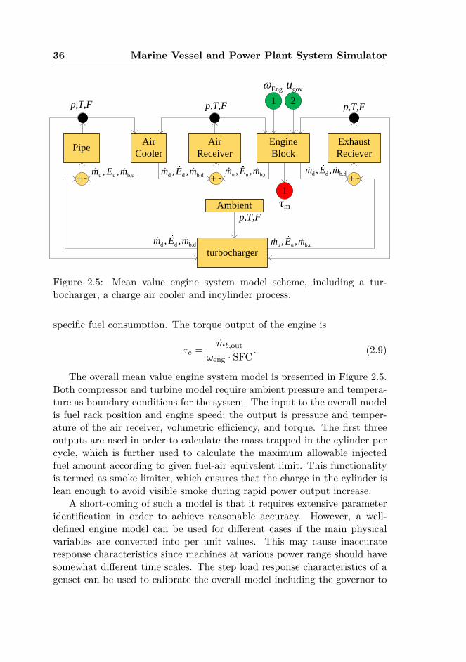
36 Marine Vessel and Power Plant System Simulator
turbocharger
PipeAir
Cooler
Air
Receiver
Engine
Block
Exhaust
Reciever
p,T,F
u u b,u, ,m E m
p,T,F p,T,F
d d b,d, ,m E mu u b,u, ,m E m
u u b,u, ,m E m d d b,d, ,m E md d b,d, ,m E m
Ambient
p,T,F
1 2
1
Eng govu
τm
+ - + - + -
Figure 2.5: Mean value engine system model scheme, including a tur-bocharger, a charge air cooler and incylinder process.
specific fuel consumption. The torque output of the engine is
τe = mb,outωeng · SFC . (2.9)
The overall mean value engine system model is presented in Figure 2.5.Both compressor and turbine model require ambient pressure and tempera-ture as boundary conditions for the system. The input to the overall modelis fuel rack position and engine speed; the output is pressure and temper-ature of the air receiver, volumetric efficiency, and torque. The first threeoutputs are used in order to calculate the mass trapped in the cylinder percycle, which is further used to calculate the maximum allowable injectedfuel amount according to given fuel-air equivalent limit. This functionalityis termed as smoke limiter, which ensures that the charge in the cylinder islean enough to avoid visible smoke during rapid power output increase.
A short-coming of such a model is that it requires extensive parameteridentification in order to achieve reasonable accuracy. However, a well-defined engine model can be used for different cases if the main physicalvariables are converted into per unit values. This may cause inaccurateresponse characteristics since machines at various power range should havesomewhat different time scales. The step load response characteristics of agenset can be used to calibrate the overall model including the governor to
2.2. Modeling 37
match the given characteristics. Such characteristics can be found in themanufacturer’s documentation, e.g. MAN Engines and Systems (2013).
Rate Constrained Model
A simplified model can be used for engines where the fuel rate is constrainedsuch that the combustion is complete. In Section 2.3.3, simulations showthat this is the case for maritime engines due to the conservative rate con-straints set by the engine manufacturers. A simplified model that ignoresthe air dynamics and requires only one parameter is
τm = kuu, (2.10)
where τm is the torque output of the diesel engine, and ku is the gain fromfuel rate to mechanical torque.
Shaft Speed Dynamics
The engine shaft speed dynamics is given by
θ = ωωb, (2.11)
ω = 12H (−Dfω + τm − τe) , (2.12)
where θ is the mechanical angle, ω is the per unit mechanical angular ve-locity, ωb is the base mechanical angular velocity, and the windage frictionconstant is denoted Df . This is derived by the swing equation and assuminglinear damping. H is defined as
H = 12Jω2
b
Pb, (2.13)
where J is the rotational inertia of the generator set and Pb is the basepower of the generator set (Krause et al.; 2013).
Governor
The two engine models use the same governor, which is based on droopcontrol (Woodward; 2004). The commanded fuel index is then calculatedby a PID controller with back calculation to avoid wind-up of the integra-tor term. The derivative of the frequency is calculated by using the dirty
38 Marine Vessel and Power Plant System Simulator
derivative.
ωref = ωNL −Kdroopp, (2.14)u = Kp(ωref − ω) +Kiξ −Kdω, (2.15)ξ = ωref − ω +Kb(usaturated − u), (2.16)˙ω = N(ω − ω), (2.17)
where the Kd, Ki, Kp, and Kb are the nonnegative derivative, integration,proportional, and back-calculation gain. The per unit produced generatorpower is denoted p. The symbols ωref , ωNL, and ω are the reference fre-quency, setpoint no-load frequency, and estimated time derivative of thefrequency.
For the rate constrained model, an additional constraint on the fuelindex is needed to avoid too large temperature variations in the cylinderand sooting due to too little air for complete combustion. This constraint ispredefined and, therefore, static. In the case study, the engine is allowed toincrease the fuel index with 20% of the rated output and then increase thefuel index with 8.1%/s. This is found by tuning the engine model response tofit recovery time and frequency drop in MAN Engines and Systems (2013).
For the mean value model, a smoke limiter constrains the governor’scommand. The amount of air available for a cycle is
mair = ηvolpARVd
RTAR, (2.18)
where ηvol is the volumetric efficiency, pAR and TAR are the pressure andtemperature at an air receiver, R is the specific gas constant and Vd is thedisplacement volume of a cylinder. Given the maximum fuel-air equivalentratio, Fmax, the maximum fuel index, umax, is given by
umax = mairFmaxfs
mf,inj, (2.19)
where fs is the stoichiometric fuel-air ratio and mf,inj is the amount ofmaximum fuel injection per cycle. In the case study, Fmax is chosen as 1 inorder to give a reasonable engine response.
2.2.6 Energy Storage Devices
ESDs include batteries, capacitors, fuel cells, or any other device capableof providing and consuming power on demand. They are accounted for by
2.2. Modeling 39
the PMS as available power reserve, and depending on the control strategyadopted by the PMS, it might substitute a fast load reduction strategy.The inner dynamics in the energy storage devices are disregarded, since it isassumed that its dynamics are much faster than the remaining components.
All components included here are simplified, since the losses are modeledusing an efficiency table. This method makes it simple to include and modelmore components with data provided by the manufacturers.
2.2.7 Thrusters
The thrusters are modeled as propellers which are driven by electrical mo-tors. The propellers are assumed to be fixed pitch, while the speed is vari-able. No thruster-thruster or thruster-hull interaction losses are included.It is assumed that the torque of the electrical motor is perfectly controlled.A frequency converter is often used to control the motor. The time scale ofthe dynamics of the frequency converter is much faster than the dynamicsof the mechanical part of the thruster drives, and it is therefore neglected.A speed controller is used to control the thrust. The open water charac-teristics are used to calculate the desired shaft speed, from the requestedthrust. The thrust is given by (Sørensen; 2013)
Ta = sign(n)KTρD4n2, (2.20)
where KT is the thrust coefficient found from open water tests, ρ is thedensity of water, D is the propeller diameter, and n is the shaft speed. Thisgives the desired shaft speed
nd = sign(Td)√|Td|
KTρD4 . (2.21)
The desired thrust signal must be smoothed since the desired thrust istypically calculated at 1 Hz. Large power fluctuation will occur at eachthruster command update instant if this is not done. A second order filteris therefore used for this task.
The four-quadrant model of the propeller presented in Smogeli (2006), isused to calculate the actual thrust and torque of the thruster. The benefitof this model is that it models wind milling (i.e., shaft speed and torquehave different signs). The advance velocity of the propeller is assumed to beequal to the relative velocity of the vessel. This means that wave-propellerinteraction due to vessel motion is included, but wave-propeller interaction
40 Marine Vessel and Power Plant System Simulator
due to wave-induced particle motion is not included (Sørensen and Smogeli;2009).
This model was first presented by Miniovich (1960). The thrust andtorque coefficients are defined as
CT = Ta12πR
2ρV 20.7, (2.22)
CQ = Qa12πR
3ρV 20.7, (2.23)
where Ta is the thrust, R is the radius of the propeller, and Qa is thepropeller torque. V0.7 is the undisturbed incident velocity to the propellerblade at radius 0.7R and is defined as
V0.7 =√Va + (0.7ωR)2, (2.24)
where ω is the angular velocity of the propeller shaft.The angle of attack of the propeller at 0.7R, β, is defined as
β = arctan(
Va
0.7ωR
). (2.25)
To estimate CT and CQ, a Fourier approximation as a function of β is used,with parameters from Smogeli (2006).
The power consumption of the thrusters are typically reduced after afault by the fast load reduction. This is done by limiting the torque ofthe electrical motor driving the propeller. In practice, this is done by thefrequency converter.
The thrust allocation needs an estimate of the power consumption ofthe thrusters. The four-quadrant model is not suitable for this purpose, asthe advance velocity is not available for the thrust allocation. The powerconsumption by the electric thruster is therefore approximated by
p = k|f |1.5, (2.26)
where f is the thrust amplitude, and k is a constant which can be found frombollard pull test results or open water tests (Sørensen; 2013, Chapter 9).Due to the approximation, the actual and approximated power consumptionmay be different.
2.3. Verification 41
2.2.8 Other Components
The last model in the electrical power simulator is a block named other loads.It represents loads that do not directly influence the propulsion system andare modeled as time series of desired and actual power consumption. Theload is divided into two parts: high and low priority loads. Both send adesired power consumption to the PMS. The PMS will then allocate poweravailable back to these loads. The PMS will first allocate power to the highpriority loads, which may be an emergency system. The thrusters will thenget allocated the remaining power, before the low priority loads get the lastremaining available power. The actual consumed power is set equal to theallocated power available.
2.2.9 Vessel, Environment, Observer, and DP Controller
Models from the MCSim toolbox and MSS toolbox (Perez et al.; 2006) areused to model the vessel. In the simulation cases we have chosen mod-els suitable for DP operations. The MSS toolbox contains multiple vesselmodels, and the model should be chosen depending on the simulation case.
MCSim is a high fidelity vessel model for low speed simulations, whichincludes wave frequency motions and low frequency motions. The low fre-quency motions includes forces from slowly varying current, second orderwave drift, mean wind, and wind gust, in addition to hydrodynamic andthruster forces from the vessel. Wave frequency motion is found by motiontransfer functions. MCSim uses transfer functions which can be found fromWAMIT (Lee; 1995).
The state observer is a passive observer based on Fossen and Strand(1999), and the DP controller is implemented as a PID controller.
The fastest time scales of the vessel motion dynamics is the time scaleof the wind gust, around 1 seconds. The slowest time scale is the change ofthe environmental condition, this is in the order of tens of minutes to hoursor days. The environment is set constant, except for a slowly varying oceancurrent. Simulations are usually done using a shorter time horizon thanthe time scale of the change of environment condition. In such cases, theenvironment can be assumed to be constant during the simulation period.
2.3 Verification
Most of the models used in this simulator are well known models, which arealready verified. However, the electric model, the rate constrained diesel
42 Marine Vessel and Power Plant System Simulator
engine model, and the parameters of the mean value diesel engine modelneeds to be verified.
2.3.1 Electric Model
A generator model based on flux linkages is used to verify the electricmodel (Krause et al.; 2013, Section 5.11). Parameters for the model arefound in Krause et al. (2013, Table 5.10-1) and the simulations are donewith two generators connected to the same load. The generator sets areoperated with similar diesel engines, AVR, and governors for both modelsand generator sets.
For the steady-state model, the load is set to consume a constant power.The load of the flux-linkage model is set by a resistance, which gives thedesired power consumption when the voltage is at the rated value.
In Figure 2.6, the power, voltage, and frequency of the generators areplotted for a step increase of the load from 20% to 70%. Note that thesimulated power of the steady-state model fits the power consumption ofthe flux-linkage model. A drop in the power of the flux-linkage occurs sincethe resistance of the load is suddenly increased, which also gives a voltagedrop. The small difference afterward is mainly due to the different modelsof the load. The frequency is perfectly modeled, as expected since the powerresponse is close for the two models. However, the voltage is not as wellaligned during the first tenth of a second. Both models are able to capturea drop in voltage. However, while the timescale of the drop is consistentbetween the model (few milliseconds), the magnitude is inconsistent (6.3%for steady-state model and 71% for the flux-linkage model). There are alsosome sub-transients which are not captured by the steady-state model.
In order to model the voltage accurately, a high fidelity model of theload is also needed. This may be difficult for a marine vessel consisting ofmany different consumers where each consumer needs to be modeled.
2.3.2 Diesel Engine Model
A good diesel engine model should be able to predict fuel consumption aswell as the engine dynamics in terms of speed under transient loads. Itis crucial to get a correct fuel consumption curve because the model usesa prescribed cycle efficiency curve rather than actual cycle calculation inthe cylinders. Such a curve can be obtained by fitting to the given fuelconsumption data available for the engine.
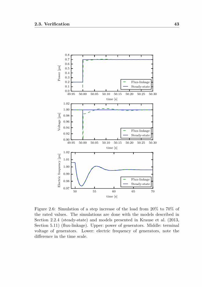
2.3. Verification 43
49.95 50.00 50.05 50.10 50.15 50.20 50.25 50.30
time [s]
0.0
0.1
0.2
0.3
0.4
0.5
0.6
0.7
0.8P
ow
er[p
u]
Flux-linkage
Steady-state
49.95 50.00 50.05 50.10 50.15 50.20 50.25 50.30
time [s]
0.90
0.92
0.94
0.96
0.98
1.00
1.02
Volt
age
[pu
]
Flux-linkage
Steady-state
50 55 60 65 70
time [s]
0.97
0.98
0.99
1.00
1.01
1.02
Ele
ctri
cfr
equ
ency
[pu
]
Flux-linkage
Steady-state
Figure 2.6: Simulation of a step increase of the load from 20% to 70% ofthe rated values. The simulations are done with the models described inSection 2.2.4 (steady-state) and models presented in Krause et al. (2013,Section 5.11) (flux-linkage). Upper: power of generators. Middle: terminalvoltage of generators. Lower: electric frequency of generators, note thedifference in the time scale.
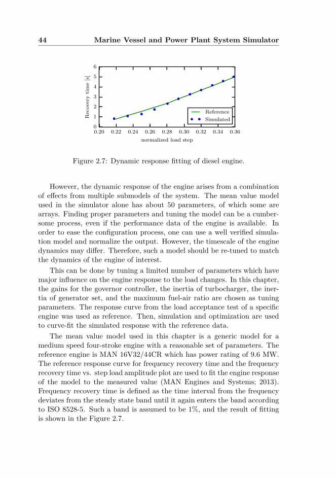
44 Marine Vessel and Power Plant System Simulator
0.20 0.22 0.24 0.26 0.28 0.30 0.32 0.34 0.36
normalized load step
0
1
2
3
4
5
6
Rec
over
yti
me
[s]
Reference
Simulated
Figure 2.7: Dynamic response fitting of diesel engine.
However, the dynamic response of the engine arises from a combinationof effects from multiple submodels of the system. The mean value modelused in the simulator alone has about 50 parameters, of which some arearrays. Finding proper parameters and tuning the model can be a cumber-some process, even if the performance data of the engine is available. Inorder to ease the configuration process, one can use a well verified simula-tion model and normalize the output. However, the timescale of the enginedynamics may differ. Therefore, such a model should be re-tuned to matchthe dynamics of the engine of interest.
This can be done by tuning a limited number of parameters which havemajor influence on the engine response to the load changes. In this chapter,the gains for the governor controller, the inertia of turbocharger, the iner-tia of generator set, and the maximum fuel-air ratio are chosen as tuningparameters. The response curve from the load acceptance test of a specificengine was used as reference. Then, simulation and optimization are usedto curve-fit the simulated response with the reference data.
The mean value model used in this chapter is a generic model for amedium speed four-stroke engine with a reasonable set of parameters. Thereference engine is MAN 16V32/44CR which has power rating of 9.6 MW.The reference response curve for frequency recovery time and the frequencyrecovery time vs. step load amplitude plot are used to fit the engine responseof the model to the measured value (MAN Engines and Systems; 2013).Frequency recovery time is defined as the time interval from the frequencydeviates from the steady state band until it again enters the band accordingto ISO 8528-5. Such a band is assumed to be 1%, and the result of fittingis shown in the Figure 2.7.
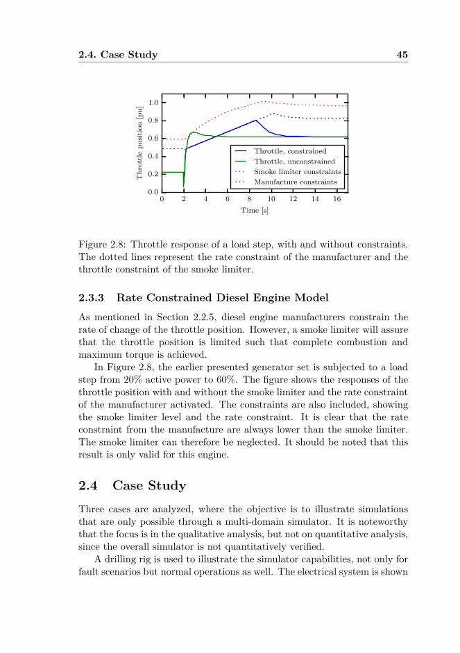
2.4. Case Study 45
0 2 4 6 8 10 12 14 16
Time [s]
0.0
0.2
0.4
0.6
0.8
1.0
Th
rott
lep
osi
tion
[pu
]
Throttle, constrained
Throttle, unconstrained
Smoke limiter constraints
Manufacture constraints
Figure 2.8: Throttle response of a load step, with and without constraints.The dotted lines represent the rate constraint of the manufacturer and thethrottle constraint of the smoke limiter.
2.3.3 Rate Constrained Diesel Engine Model
As mentioned in Section 2.2.5, diesel engine manufacturers constrain therate of change of the throttle position. However, a smoke limiter will assurethat the throttle position is limited such that complete combustion andmaximum torque is achieved.
In Figure 2.8, the earlier presented generator set is subjected to a loadstep from 20% active power to 60%. The figure shows the responses of thethrottle position with and without the smoke limiter and the rate constraintof the manufacturer activated. The constraints are also included, showingthe smoke limiter level and the rate constraint. It is clear that the rateconstraint from the manufacture are always lower than the smoke limiter.The smoke limiter can therefore be neglected. It should be noted that thisresult is only valid for this engine.
2.4 Case StudyThree cases are analyzed, where the objective is to illustrate simulationsthat are only possible through a multi-domain simulator. It is noteworthythat the focus is in the qualitative analysis, but not on quantitative analysis,since the overall simulator is not quantitatively verified.
A drilling rig is used to illustrate the simulator capabilities, not only forfault scenarios but normal operations as well. The electrical system is shown
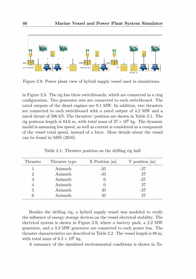
46 Marine Vessel and Power Plant System Simulator
Figure 2.9: Power plant view of hybrid supply vessel used in simulations.
in Figure 2.3. The rig has three switchboards, which are connected in a ringconfiguration. Two generator sets are connected to each switchboard. Therated outputs of the diesel engines are 9.1 MW. In addition, two thrustersare connected to each switchboard with a rated output of 4.2 MW and arated thrust of 506 kN. The thrusters’ position are shown in Table 2.1. Therig pontoon length is 84.6 m, with total mass of 27× 106 kg. The dynamicmodel is assuming low speed, as well as current is considered as a componentof the vessel total speed, instead of a force. More details about the vesselcan be found in MSS (2010).
Table 2.1: Thruster position on the drilling rig hull
Thruster Thruster type X Position [m] Y position [m]1 Azimuth -35 -272 Azimuth -35 273 Azimuth 0 -274 Azimuth 0 275 Azimuth 35 -276 Azimuth 35 27
Besides the drilling rig, a hybrid supply vessel was modeled to verifythe influence of energy storage devices on the vessel electrical stability. Theelectrical system is shown in Figure 2.9, where a battery pack, a 2.2 MWgenerator, and a 3.3 MW generator are connected to each power bus. Thethruster characteristics are described in Table 2.2. The vessel length is 80 m,with total mass of 6.2× 10⁶ kg.
A summary of the simulated environmental conditions is shown in Ta-
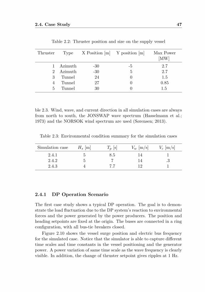
2.4. Case Study 47
Table 2.2: Thruster position and size on the supply vessel
Thruster Type X Position [m] Y position [m] Max Power[MW]
1 Azimuth -30 -5 2.72 Azimuth -30 5 2.73 Tunnel 24 0 1.54 Tunnel 27 0 0.855 Tunnel 30 0 1.5
ble 2.3. Wind, wave, and current direction in all simulation cases are alwaysfrom north to south, the JONSWAP wave spectrum (Hasselmann et al.;1973) and the NORSOK wind spectrum are used (Sørensen; 2013).
Table 2.3: Environmental condition summary for the simulation cases
Simulation case Hs [m] Tp [s] Vw [m/s] Vc [m/s]2.4.1 5 8.5 14 12.4.2 5 7 14 .32.4.3 4 7.7 12 1
2.4.1 DP Operation Scenario
The first case study shows a typical DP operation. The goal is to demon-strate the load fluctuation due to the DP system’s reaction to environmentalforces and the power generated by the power producers. The position andheading setpoints are fixed at the origin. The buses are connected in a ringconfiguration, with all bus-tie breakers closed.
Figure 2.10 shows the vessel surge position and electric bus frequencyfor the simulated case. Notice that the simulator is able to capture differenttime scales and time constants in the vessel positioning and the generatorpower. A power variation of same time scale as the wave frequency is clearlyvisible. In addition, the change of thruster setpoint gives ripples at 1 Hz.
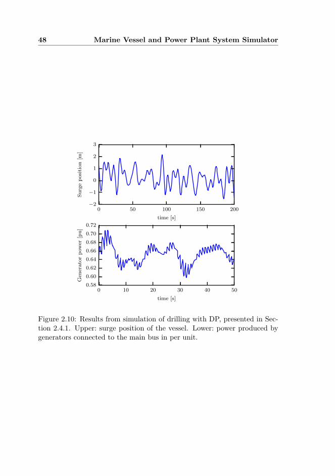
48 Marine Vessel and Power Plant System Simulator
0 50 100 150 200
time [s]
−2
−1
0
1
2
3
Su
rge
posi
tion
[m]
0 10 20 30 40 50
time [s]
0.58
0.60
0.62
0.64
0.66
0.68
0.70
0.72
Gen
erato
rp
ow
er[p
u]
Figure 2.10: Results from simulation of drilling with DP, presented in Sec-tion 2.4.1. Upper: surge position of the vessel. Lower: power produced bygenerators connected to the main bus in per unit.
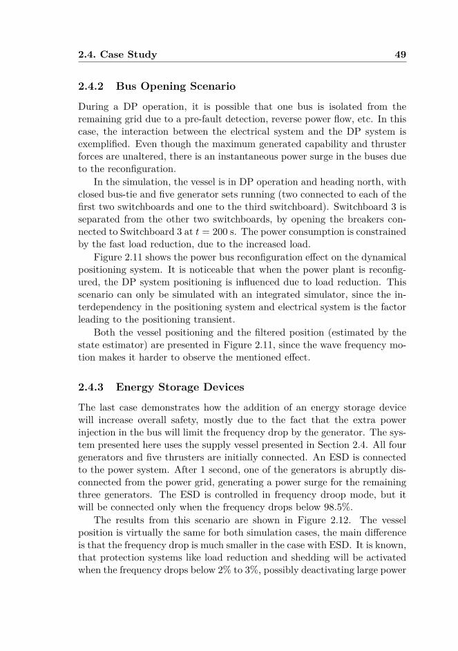
2.4. Case Study 49
2.4.2 Bus Opening Scenario
During a DP operation, it is possible that one bus is isolated from theremaining grid due to a pre-fault detection, reverse power flow, etc. In thiscase, the interaction between the electrical system and the DP system isexemplified. Even though the maximum generated capability and thrusterforces are unaltered, there is an instantaneous power surge in the buses dueto the reconfiguration.
In the simulation, the vessel is in DP operation and heading north, withclosed bus-tie and five generator sets running (two connected to each of thefirst two switchboards and one to the third switchboard). Switchboard 3 isseparated from the other two switchboards, by opening the breakers con-nected to Switchboard 3 at t = 200 s. The power consumption is constrainedby the fast load reduction, due to the increased load.
Figure 2.11 shows the power bus reconfiguration effect on the dynamicalpositioning system. It is noticeable that when the power plant is reconfig-ured, the DP system positioning is influenced due to load reduction. Thisscenario can only be simulated with an integrated simulator, since the in-terdependency in the positioning system and electrical system is the factorleading to the positioning transient.
Both the vessel positioning and the filtered position (estimated by thestate estimator) are presented in Figure 2.11, since the wave frequency mo-tion makes it harder to observe the mentioned effect.
2.4.3 Energy Storage Devices
The last case demonstrates how the addition of an energy storage devicewill increase overall safety, mostly due to the fact that the extra powerinjection in the bus will limit the frequency drop by the generator. The sys-tem presented here uses the supply vessel presented in Section 2.4. All fourgenerators and five thrusters are initially connected. An ESD is connectedto the power system. After 1 second, one of the generators is abruptly dis-connected from the power grid, generating a power surge for the remainingthree generators. The ESD is controlled in frequency droop mode, but itwill be connected only when the frequency drops below 98.5%.
The results from this scenario are shown in Figure 2.12. The vesselposition is virtually the same for both simulation cases, the main differenceis that the frequency drop is much smaller in the case with ESD. It is known,that protection systems like load reduction and shedding will be activatedwhen the frequency drops below 2% to 3%, possibly deactivating large power
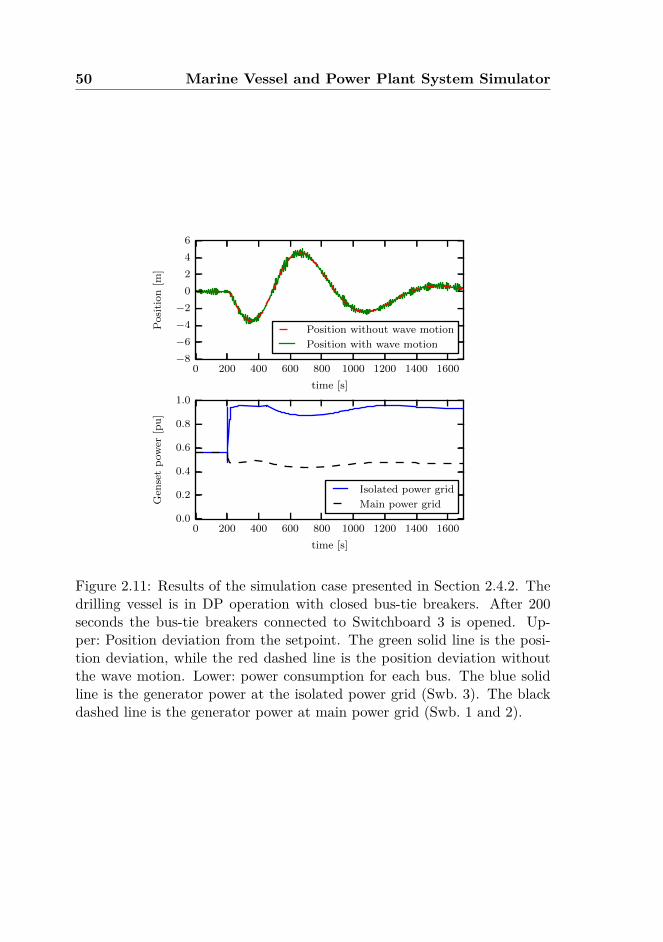
50 Marine Vessel and Power Plant System Simulator
0 200 400 600 800 1000 1200 1400 1600
time [s]
−8
−6
−4
−2
0
2
4
6
Posi
tion
[m]
Position without wave motion
Position with wave motion
0 200 400 600 800 1000 1200 1400 1600
time [s]
0.0
0.2
0.4
0.6
0.8
1.0
Gen
set
pow
er[p
u]
Isolated power grid
Main power grid
Figure 2.11: Results of the simulation case presented in Section 2.4.2. Thedrilling vessel is in DP operation with closed bus-tie breakers. After 200seconds the bus-tie breakers connected to Switchboard 3 is opened. Up-per: Position deviation from the setpoint. The green solid line is the posi-tion deviation, while the red dashed line is the position deviation withoutthe wave motion. Lower: power consumption for each bus. The blue solidline is the generator power at the isolated power grid (Swb. 3). The blackdashed line is the generator power at main power grid (Swb. 1 and 2).
2.4. Case Study 51
0 2 4 6 8 10
time [s]
0.6
0.8
1.0
1.2
1.4
1.6
1.8
2.0
Gen
erato
rp
ow
er[p
u]
with battery
without battery
0 2 4 6 8 10
time [s]
0.94
0.95
0.96
0.97
0.98
0.99
1.00
Fre
qu
ency
[pu
]
with battery
without battery
Figure 2.12: Results from presented in Section 2.4.3. After 1 second one outof four generator is disconnected. Upper: generator power, with and with-out battery. Lower: electric frequency of the main bus, with and withoutbattery.
consumers, such as thrusters, drilling system, etc. If the frequency dropseven further, it could lead to partial or even total blackout.
From the maintenance point of view, with smoother generator load vari-ation, the wear and tear will be reduced, improving the generator workingconditions and reducing maintenance costs.
This simulation shows that the simulator allows investigating the vesseland ESD dynamical behavior during a fault, in which the frequency drop isthe main concern. The ESD is able to bound the frequency drop to a safemargin, potentially preventing a larger scale fault.
Other operation strategies may be implemented for the ESD, such aspeak shaving, on-off operations, etc., if the simulator is properly set up.
52 Marine Vessel and Power Plant System Simulator
2.5 ConclusionIn this chapter, a simulator for marine vessels electric propulsion is pre-sented. The main contribution is the presentation and verification of theneeded models for the integration of power plant simulation and vessel mo-tion simulation. In addition to demonstrations of the integrated simulator,enabling qualitative analysis of cases that cannot be described with sev-eral decoupled simulators. Detailed models of the vessel, propeller, thrusterdrives, generator sets, and controllers are included in the system simulator,in addition to interaction effects between the components. A module basedplatform is presented, where models of different fidelity can be chosen. Dueto the modularity, the simulator can be reconfigured to different vessels withelectric propulsion, and different operations can be simulated. Simulink wasused to implement the simulator. The case studies presented in the chaptershow some capabilities of the simulator. More detailed simulations of, forinstance, fault scenarios contribute to increased knowledge about the be-havior of the electrical system, control systems, and safety functions. Thismay lead to more reliable vessels and safer operations in the future.
Chapter 3
Dynamic ConsequenceAnalysis of Marine ElectricPower Plant in DynamicPositioning
This chapter is based on Bø et al. (n.d.).
Introduction
Dynamic positioning (DP) systems are used for stationkeeping of marinevessels. The general safety requirement for classes 2 and 3 is that any sin-gle fault should not propagate into a loss of position (IMO; 1994). This isenabled by redundancy, which means that if one redundancy group fails,remaining redundancy-groups have sufficient capacity to maintain station-keeping.
An online consequence analysis is required for DP vessels of classes 2and 3 (IMO; 1994, Section 3.2.4.2). The IMO rules state that: “This anal-ysis should verify that the thrusters remaining in operation after the worstcase failure can generate the same resultant thruster force and moment asrequired before the failure.” An alarm should be raised if this verificationis negative. Another tool is DP capability plots, which are used to de-termine the environmental limits of an operation. These plots show themaximum static or quasi-static wind, current, and wave loads in which thevessel can maintain its position, for all headings and different configura-
53
54Dynamic Consequence Analysis of Marine Electric Power Plant
in Dynamic Positioning
tions (e.g., worst-case, nominal case). Specifications of this plot are givenin IMCA (2000). Drift-off analysis is used during drilling operations to de-termine when to initiate the disconnection of the riser from the vessel toavoid damage to the riser (ISO; 2009). Because, disconnection process ofa riser during a drift-off is time consuming (e.g., in case of a blackout), awatch circle is set such that there is sufficient time to safely disconnect theriser if the process is started when the vessel passes the watch circle.
A power management system (PMS) is used for controlling the electricalpower system. The main task of the PMS is to ensure the sufficient availabil-ity of power. In addition, the PMS coordinates fault recovery and typicallyoptimizes the efficiency of a power plant. In the case of a major fault, loadsmust be quickly reduced to prevent the occurrence of under-frequency, be-cause it takes time for diesel engines to increase their produced power. ThePMS sends a power available signal to main consumers to ensure that onlyavailable power is used. This is the maximum allowed power for each con-sumer. It is calculated by acquiring the available power production levelof each generator set and then allocating it to consumers based on theirpriority. Fast load reduction may be used when sudden load reduction isrequired (e.g., loss of producers), which sends a request to thruster drivesto reduce their power. This proceeds as thruster drives can quickly reducepower consumption. Later, the available power of thrusters is increasedback to normal.
In Pivano et al. (2014), a simulation-based consequence analysis is pro-posed. Notably, conventional DP capability analysis is non-conservativecompared with time-domain analysis. Moreover, power constraints andtransient recovery after faults are not considered in their analysis. A tran-sient study was also performed, which showed that position excursion maybe larger than acceptable during the transient recovery after a fault.
Recently, it has been proposed by the DNV GL DYNPOS-ER classnotation that standby generators can be included in a consequence analy-sis (DNV; 2015, Part 6 Chapter 26 Section 2). Other class societies havesimilar class notations, e.g., ABS (2014, Section 8). Because the connectionof generators can be blocked by hidden faults, it is conservatively assumedthat one of the standby generators cannot connect because of a hidden fault.This provides the opportunity to run relatively few generator sets, whichincreases the efficiency of a plant. Typically, a marine diesel engine is at itshighest efficiency when it delivers about 80% of its rated power. However, itis reported that during DP operations, diesel engines often deliver less than50% and even down to 10% of the rated power. Moreover, during low-load
55
conditions, other problems occur, such as sooting, increased maintenancebecause of extra running hours, and inefficiency of some NOX reductionsystems at low temperatures (Realfsen; 2009).
The analysis proposed in this chapter can also be used as a decision-support tool for the optimal configuration of a vessel. Several configurationscan be simulated to evaluate the safety and performance of each configura-tion. Today, an automatic start and stop table is typically used for commit-ment of generators on marine vessels (Ådnanes; 2003). Generator sets arestarted if the power demand is above a threshold for a certain duration oftime, vice versa for disconnection. An optimized load-dependent start tablewas derived in Radan et al. (2005), where the table was optimized with re-spect to fuel consumption and constrained by a safety requirement, so thatdisconnection of a generator will not lead to blackout. Algorithms to opti-mize the load-dependent start and stop tables are also presented in Radanet al. (2006), based on the probability for each operational mode of thevessel. One of the problems with a start and stop table is its independenceof operation. For diving and drilling vessels, the safety and redundancyrequirements are much higher during operation than during transit. How-ever, when using a start and stop table both operations will typically havethe same configuration when the power demand is similar, even though thisis not optimal. Therefore, some vessels have different start/stop tables foreach mode and also a minimum number of generator sets for some modes tohandle changing requirements. It is also common to override the automaticsystem by committing generators manually. For onshore and island powergrids, multiple studies have looked into unit commitment, e.g., Contaxis andKabouris (1991); Dillon et al. (1978); Dokopoulos and Saramourtsis (1996);Juste et al. (1999); Lowery (1966); Senjyu and Shimabukuro (2003).
The main contribution of this chapter is the development of a conse-quence analysis based on dynamic simulation of the transient recovery aftera fault. The analysis is carried out by dynamic time-domain simulation ofthe vessel and its DP system for possible worst single failures. The simula-tions include power constraints and ramp constraints on the thrusters. Thistool can also be used as a decision-support system for configuration of thepower plant and selection of recovery-methods.
The chapter is divided into two sections. The method is presented inthe first section and the second section presents a case study considering adrilling rig. The first section starts with an overview of the method followedby a presentation of the simulator. In Section 3.1.3, the fault models arepresented, followed by acceptance criterion and environmental models. The
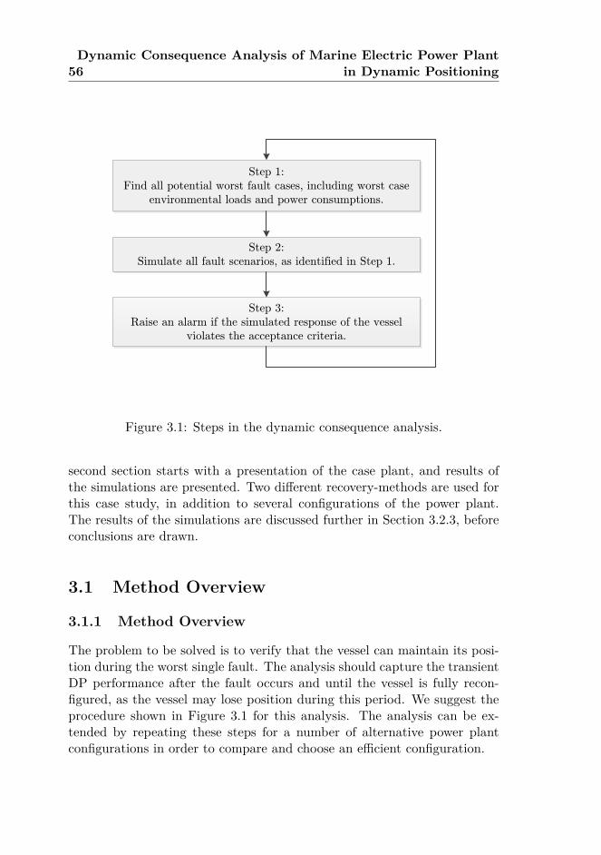
56Dynamic Consequence Analysis of Marine Electric Power Plant
in Dynamic Positioning
Step 1:
Find all potential worst fault cases, including worst case
environmental loads and power consumptions.
Step 2:
Simulate all fault scenarios, as identified in Step 1.
Step 3:
Raise an alarm if the simulated response of the vessel
violates the acceptance criteria.
Figure 3.1: Steps in the dynamic consequence analysis.
second section starts with a presentation of the case plant, and results ofthe simulations are presented. Two different recovery-methods are used forthis case study, in addition to several configurations of the power plant.The results of the simulations are discussed further in Section 3.2.3, beforeconclusions are drawn.
3.1 Method Overview
3.1.1 Method Overview
The problem to be solved is to verify that the vessel can maintain its posi-tion during the worst single fault. The analysis should capture the transientDP performance after the fault occurs and until the vessel is fully recon-figured, as the vessel may lose position during this period. We suggest theprocedure shown in Figure 3.1 for this analysis. The analysis can be ex-tended by repeating these steps for a number of alternative power plantconfigurations in order to compare and choose an efficient configuration.
3.1. Method Overview 57
3.1.2 Simulator
A dynamic simulator of the electric power plant and marine vessel is used.The simulator in this study should be regarded as an example implementa-tion. Details of the simulator are given in Bø et al. (2015). We are mainlyinterested in the response of the DP-system due to faults in the power sys-tem. Hence, the implemented models are chosen to represent the DP-systemas realistically as possible, with its algorithms, tuning, and constraints. Thepower system is included as it constrains the DP-system during fault recov-ery. The main components of the simulator are:
Vessel: A 6 DOF model is used to describe the motion of the vessel. Themotion is divided into low-frequency motion and first-order wave fre-quency motion. The low-frequency motion includes non-linear drag,second-order mean and slowly varying wave, current, wind, and thrusterloads. The first-order wave frequency motion is calculated from thewave spectrum and response amplitude operator (RAO) of the vessel.
Environmental Load: The wave spectrum used in this study is JON-SWAP with a narrow banded directional spectrum, although any otherwave spectrum could be used. This is used to generate discrete waves,which are used to calculate the second-order wave loads. The wind andcurrent are modeled with constant speed and direction. The choice ofenvironmental conditions is further discussed in Section 3.1.5.
Dynamic Positioning System: The DP controller is implemented as aPID-controller. The position and velocity are given directly from thelow-frequency motion of the vessel, assuming an accurate heading andposition reference system. This is discussed further in Section 3.1.5.
Thrust Allocation: The DP controller calculates a total thrust commandfor the vessel, the thrust allocation (TA) then allocates a thrust com-mand for each thruster. This is an optimization problem, constrainedby the available power.
Power Management System: A PMS is included to simulate the con-trol of power generation and distribution. It includes power availableallocation and fast load reduction.
Thrusters: The thruster model includes models of the motor drive, electricmotor, propeller, and the local thruster controller. A four-quadrantmodel is used to calculate the thrust and torque on the propeller. The
58Dynamic Consequence Analysis of Marine Electric Power Plant
in Dynamic Positioning
power consumption of the thrusters can be constrained by the PMSand the thrust allocation, this limits the power of the electric thrustermotor.
Electric System: The electric system is assumed to be in steady state,as the mechanical systems in a diesel-electric propulsion system aremuch slower than the electric system. The modeled variables are fre-quency, voltage, active power, and reactive power. This allows us tosimulate the power flow and power constraints. However, fast dynam-ics, such as short-circuit and harmonic distortions, are not included inthe model. Some protection relays are included in the model, such asunder/over-frequency protection and reverse-power protection. How-ever, as fast dynamics are not modeled, protection relays based onvoltage measurements are not included.
Generator Set: The generator set consists of a diesel engine and a syn-chronous generator. The fuel injection of the diesel engine is con-strained by a rate constraint. This engine protection is typically usedto avoid large thermal stress. The fuel consumption is calculated bya Willans approximation (Guzzella and Onder; 2010). All other fueldynamics are ignored in this study, due to the conservative rate con-straint. A governor is used to control the load sharing and speed ofthe engine. Typically, the governors use droop or isochronous controlfor the load sharing. An automatic voltage regulator is used to controlthe voltage and reactive power sharing.
Electric Loads: Loads other than thrusters and heave compensators aremodeled as a time-series. These may be hotel loads, auxiliary loads,drilling drives, and cranes. These loads are prioritized, either aboveor below thruster loads in the PMS. Low-priority loads are reduced ifthe available power is not sufficient. However, high-priority loads willonly be reduced if it is not sufficient to reduce both low-priority loadsand thruster loads.
Heave compensators: Heave compensators are included in the model.The electric power consumption is proportional to the heave velocitywhen the velocity is positive, and zero when the velocity is negative.They may be assigned high-priority in the PMS.
A marine vessel simulator consists of hundreds of parameters and statesthat need to be initialized. These should be found automatically and may
3.1. Method Overview 59
come directly from the status of the vessel. In addition, some values mustbe predicted, such as the electric power consumption and environmentalconditions. As the power constraint on the thrusters is indirectly depen-dent on the power consumption of the other consumers, it is important thatthe predicted mean and variation of the power consumption are not under-estimated. The power consumption of all electric loads, except thrustersand heave compensators, can be recorded and used as the load case in thesimulation. However, a safety-factor may be used to include uncertaintiesof the future load.
The simulator must be able to run much faster than real-time to be ableto return results that are not outdated before they are completed, becauseof this the consequence analysis should be performed online as the operationand environment may be constantly changing. Several simulations can runin parallel to increase the performance, since the scenarios are independentof each other.
The simulations are started with the vessel’s systems in a steady state.This is to make sure that the controllers, such as the I-term in the DP’sPID-controller, have settled.
3.1.3 Fault Modeling
The simulated cases should include all potential worst-case scenarios basedon faults in the power plant and thruster system, and may be identified by areport of the DP system’s failure mode and effects analysis (FMEA) (DNV;2012) or hardware-in-the-loop testing (Altosole et al.; 2009; Johansen andSørensen; 2009). This could, for example, be faults such as loss of switch-board, loss of bus segment, loss of thruster, loss of generator set, fault ingovernor, frozen command signal, or equipment delivering maximum capac-ity when this is not desired (e.g., full thrust in drive-off). Incidents reportsreveal that other causes, independent of the power plant, are as important,such as human error, faults in the reference system, and faults in the DPcontrol systems (IMCA; 1995–2011; Kristiansen; 2014). Subsystem faults,such as faults in the auxiliary systems, are not considered when selectingfault scenarios, but the worst-case consequence of such faults should beconsidered, for example, shut down of a diesel engines due to faults in theauxiliary systems.
Only single faults are considered, and it is assumed that all protectionsystems are handling the fault as designed. Therefore, common mode andsoftware faults are ignored in this study, as common mode faults should bedetected by FMEA during the design of the system. HIL-testing can also
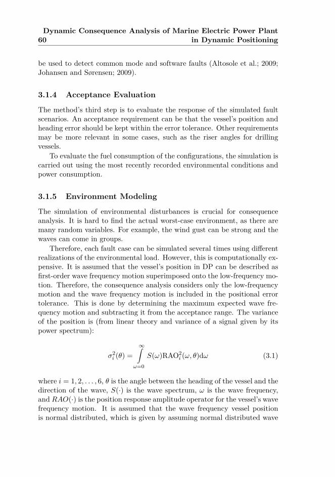
60Dynamic Consequence Analysis of Marine Electric Power Plant
in Dynamic Positioning
be used to detect common mode and software faults (Altosole et al.; 2009;Johansen and Sørensen; 2009).
3.1.4 Acceptance Evaluation
The method’s third step is to evaluate the response of the simulated faultscenarios. An acceptance requirement can be that the vessel’s position andheading error should be kept within the error tolerance. Other requirementsmay be more relevant in some cases, such as the riser angles for drillingvessels.
To evaluate the fuel consumption of the configurations, the simulation iscarried out using the most recently recorded environmental conditions andpower consumption.
3.1.5 Environment Modeling
The simulation of environmental disturbances is crucial for consequenceanalysis. It is hard to find the actual worst-case environment, as there aremany random variables. For example, the wind gust can be strong and thewaves can come in groups.
Therefore, each fault case can be simulated several times using differentrealizations of the environmental load. However, this is computationally ex-pensive. It is assumed that the vessel’s position in DP can be described asfirst-order wave frequency motion superimposed onto the low-frequency mo-tion. Therefore, the consequence analysis considers only the low-frequencymotion and the wave frequency motion is included in the positional errortolerance. This is done by determining the maximum expected wave fre-quency motion and subtracting it from the acceptance range. The varianceof the position is (from linear theory and variance of a signal given by itspower spectrum):
σ2i (θ) =
∞∫ω=0
S(ω)RAO2i (ω, θ)dω (3.1)
where i = 1, 2, . . . , 6, θ is the angle between the heading of the vessel and thedirection of the wave, S(·) is the wave spectrum, ω is the wave frequency,and RAO(·) is the position response amplitude operator for the vessel’s wavefrequency motion. It is assumed that the wave frequency vessel positionis normal distributed, which is given by assuming normal distributed wave
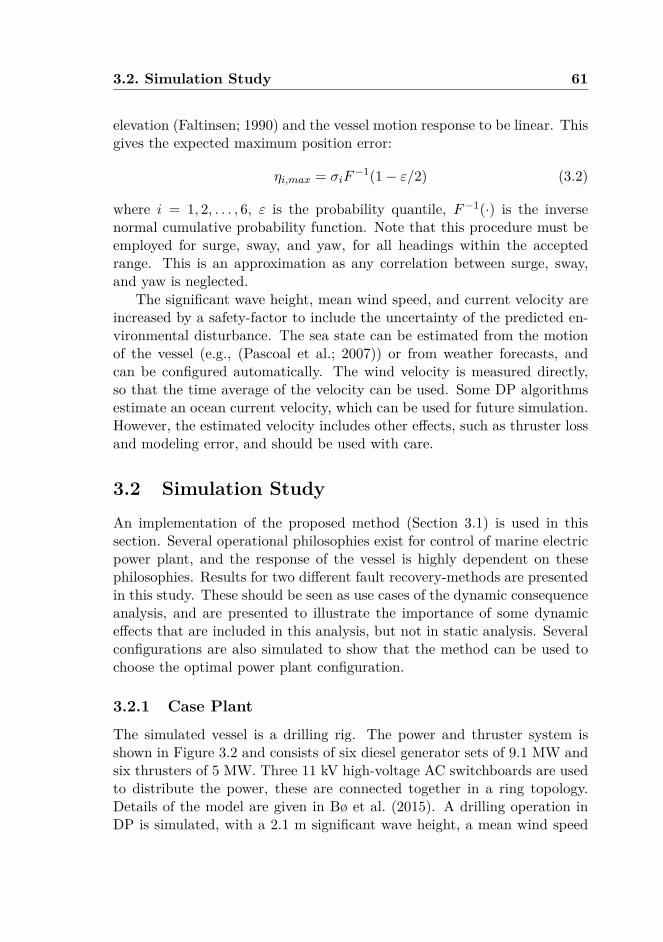
3.2. Simulation Study 61
elevation (Faltinsen; 1990) and the vessel motion response to be linear. Thisgives the expected maximum position error:
ηi,max = σiF−1(1− ε/2) (3.2)
where i = 1, 2, . . . , 6, ε is the probability quantile, F−1(·) is the inversenormal cumulative probability function. Note that this procedure must beemployed for surge, sway, and yaw, for all headings within the acceptedrange. This is an approximation as any correlation between surge, sway,and yaw is neglected.
The significant wave height, mean wind speed, and current velocity areincreased by a safety-factor to include the uncertainty of the predicted en-vironmental disturbance. The sea state can be estimated from the motionof the vessel (e.g., (Pascoal et al.; 2007)) or from weather forecasts, andcan be configured automatically. The wind velocity is measured directly,so that the time average of the velocity can be used. Some DP algorithmsestimate an ocean current velocity, which can be used for future simulation.However, the estimated velocity includes other effects, such as thruster lossand modeling error, and should be used with care.
3.2 Simulation Study
An implementation of the proposed method (Section 3.1) is used in thissection. Several operational philosophies exist for control of marine electricpower plant, and the response of the vessel is highly dependent on thesephilosophies. Results for two different fault recovery-methods are presentedin this study. These should be seen as use cases of the dynamic consequenceanalysis, and are presented to illustrate the importance of some dynamiceffects that are included in this analysis, but not in static analysis. Severalconfigurations are also simulated to show that the method can be used tochoose the optimal power plant configuration.
3.2.1 Case Plant
The simulated vessel is a drilling rig. The power and thruster system isshown in Figure 3.2 and consists of six diesel generator sets of 9.1 MW andsix thrusters of 5 MW. Three 11 kV high-voltage AC switchboards are usedto distribute the power, these are connected together in a ring topology.Details of the model are given in Bø et al. (2015). A drilling operation inDP is simulated, with a 2.1 m significant wave height, a mean wind speed
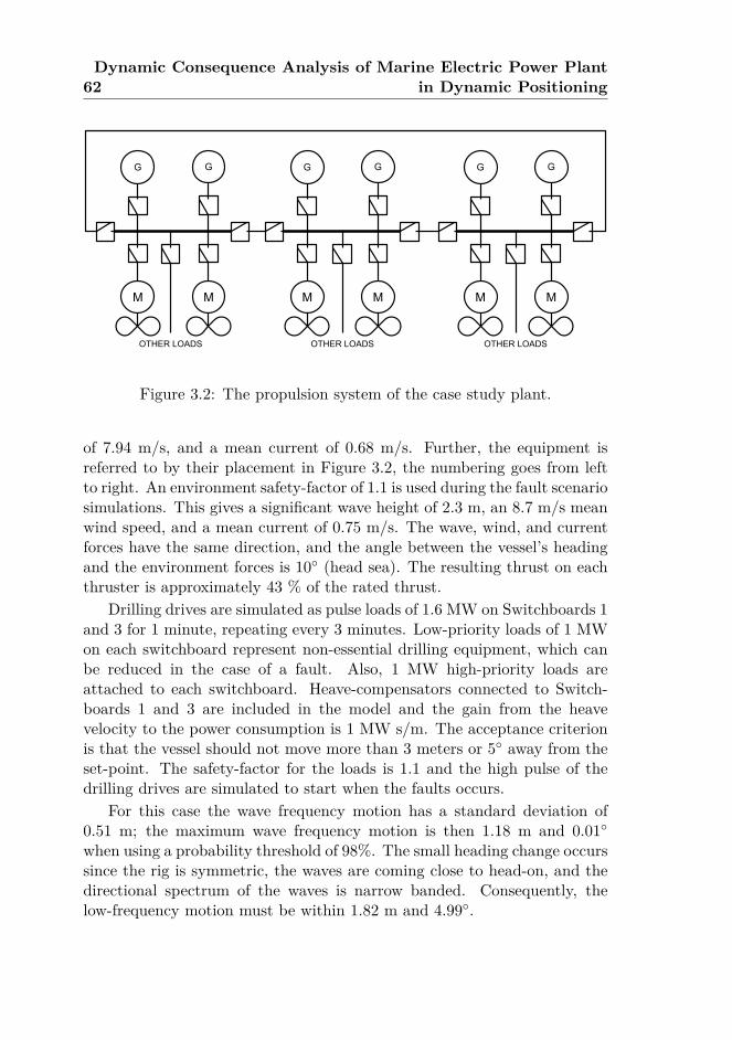
62Dynamic Consequence Analysis of Marine Electric Power Plant
in Dynamic Positioning
G
M
G
M
G
M
G
OTHER LOADS
M
G
M
G
M
OTHER LOADS OTHER LOADS
Figure 3.2: The propulsion system of the case study plant.
of 7.94 m/s, and a mean current of 0.68 m/s. Further, the equipment isreferred to by their placement in Figure 3.2, the numbering goes from leftto right. An environment safety-factor of 1.1 is used during the fault scenariosimulations. This gives a significant wave height of 2.3 m, an 8.7 m/s meanwind speed, and a mean current of 0.75 m/s. The wave, wind, and currentforces have the same direction, and the angle between the vessel’s headingand the environment forces is 10 (head sea). The resulting thrust on eachthruster is approximately 43 % of the rated thrust.
Drilling drives are simulated as pulse loads of 1.6 MW on Switchboards 1and 3 for 1 minute, repeating every 3 minutes. Low-priority loads of 1 MWon each switchboard represent non-essential drilling equipment, which canbe reduced in the case of a fault. Also, 1 MW high-priority loads areattached to each switchboard. Heave-compensators connected to Switch-boards 1 and 3 are included in the model and the gain from the heavevelocity to the power consumption is 1 MW s/m. The acceptance criterionis that the vessel should not move more than 3 meters or 5 away from theset-point. The safety-factor for the loads is 1.1 and the high pulse of thedrilling drives are simulated to start when the faults occurs.
For this case the wave frequency motion has a standard deviation of0.51 m; the maximum wave frequency motion is then 1.18 m and 0.01when using a probability threshold of 98%. The small heading change occurssince the rig is symmetric, the waves are coming close to head-on, and thedirectional spectrum of the waves is narrow banded. Consequently, thelow-frequency motion must be within 1.82 m and 4.99.

3.2. Simulation Study 63
Table 3.1: Alternative configurations. A dash — and a vertical bar | are usedto denote when switchboards are connected or disconnected via a closed oropen bus tie-breaker, respectively.
# connectedgensets per
swb.Configuration 1 2 3 Swb. groups
1 1 1 1 1 — 2 — 32 2 1 1 1 | 2 — 33 2 1 1 1 — 2 — 34 2 2 1 1 | 2 — 35 2 2 1 1 — 2 — 36 2 2 2 1 | 2 | 37 2 2 2 1 — 2 — 3
The configurations tested are shown in Table 3.1. Many more configu-rations are possible, e.g., open bus tie-breakers and one generator set perswitchboard. However, these were chosen as they give sufficient power andrepresent a broad spectrum of configurations.
The following fault cases are simulated:
1. Loss of a generator set: a generator set is disconnected. Stand-bygenerator sets, if any, are connected after 45 seconds.
2. Loss of a thruster: Thruster 1 (left most) is disconnected.
3. Loss of a switchboard: both generators and all loads connected toSwitchboard 1 (left most) are disconnected. Stand-by generator setsare connected to the healthy switchboards after 45 seconds.
4. Thruster full thrust: the thrust of Thruster 1 (left most) is fixed atfull thrust. The thruster is disconnected after two minutes.
For Cases 1, 2, and 4 the PMS is configured to only reduce thruster loads.This is an example of an operational philosophy used to avoid frequent minorfaults influencing the operation. During Case 3, it is simulated that thebus tie-breakers (directly or indirectly) connected to the faulty switchboardare opened. This strategy is typically used to avoid propagation of faultsfrom one switchboard to the others. These faults are considered as possibleworst-case scenarios for this simulated vessel. Note that Cases 1, 2, and 3are possible drift-off cases, while Case 4 is a possible drive-off case.
64Dynamic Consequence Analysis of Marine Electric Power Plant
in Dynamic Positioning
The generators are running in droop mode with equal settings. Thisgives equal load sharing among the generators connected in each group.A fast phase back system (FPBS) is implemented on the thrusters basedon May (2003). The load reduction is initiated when the frequency fallsbelow 95% of the rated frequency, the power is reduced linearly, and fullyreduced at 92.5%.
Two fault recovery-methods are simulated. In Recovery A, fast loadreduction and power available signal are used to make sure that the vesselis able to avoid under-frequency due to overload. In Recovery B, thesemethods are deactivated. Then, the power plant can use the rotating energyof the generator set during this recovery, and load reduction is only initiatedthrough FPBS. This gives less of a safety-margin against under-frequency,which increases the risk of blackout. Many other fault recovery-methodsexist, such as power limit ramps on consumers instead of available power,and the selection of bus tie-breakers to open when the switchboards fails.
3.2.2 Simulation Results
Results from nominal and fault simulations are shown in Table 3.2. Theloss of position distance is the maximum distance from the reference pointto the low-frequency position of the vessel during the simulation.
Recovery A: Power Available
For Recovery A, Configurations 2, 4, 6, and 7 are accepted, while the oth-ers fail due to loss of position during the transient recovery after a fault.Configuration 2 may be preferred as it gives the lowest fuel consumption.
The position and heading error is shown in Figure 3.3, for Configura-tions 2 and 3 after the loss of Switchboard 1. For Configuration 2, the bustie-breaker between Switchboards 2 and 3 is closed after the fault, whileit opens for Configuration 3 (since it is indirectly connected to the faultyswitchboard). A large transient position error occurs for Configuration 3after the fault, although both configurations are able to stabilize the vesselto the reference after the fault. This is a case where a transient simulationis necessary to determine the safety of the configuration. The reason for thedifference between the configurations is that the available power of a gener-ator set is dependent on the load of the generator. Therefore, the availablepower for the thrusters will differ, as seen in Figure 3.5. When using closedbus-tie and equal droop settings, all the generators produce equal amountsof power before the fault. For Configuration 3 (closed bus) this means that
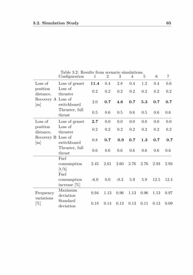
3.2. Simulation Study 65
Table 3.2: Results from scenario simulations.Configuration 1 2 3 4 5 6 7
Loss ofpositiondistance,Recovery A[m]
Loss of genset 11.4 0.4 2.8 0.4 1.2 0.4 0.6Loss ofthruster 0.2 0.2 0.2 0.2 0.2 0.2 0.2
Loss ofswitchboard 2.0 0.7 4.6 0.7 5.3 0.7 0.7
Thruster, fullthrust 0.5 0.6 0.5 0.6 0.5 0.6 0.6
Loss ofpositiondistance,Recovery B[m]
Loss of genset 2.7 0.0 0.0 0.0 0.0 0.0 0.0Loss ofthruster 0.2 0.2 0.2 0.2 0.2 0.2 0.2
Loss ofswitchboard 0.8 0.7 0.9 0.7 1.3 0.7 0.7
Thruster, fullthrust 0.6 0.6 0.6 0.6 0.6 0.6 0.6
Fuelconsumption[t/h]
2.45 2.61 2.60 2.76 2.76 2.93 2.93
Fuelconsumptionincrease [%]
-6.0 0.0 -0.3 5.9 5.9 12.5 12.4
Frequencyvariations[%]
Maximumdeviation 0.94 1.13 0.96 1.13 0.96 1.13 0.97
Standarddeviation 0.18 0.14 0.13 0.13 0.11 0.13 0.09
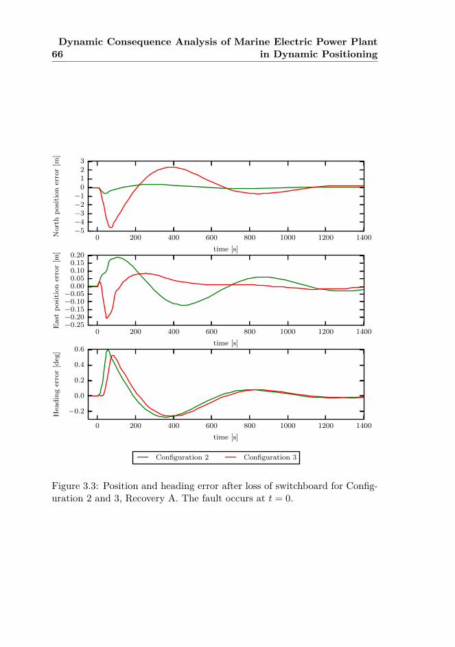
66Dynamic Consequence Analysis of Marine Electric Power Plant
in Dynamic Positioning
0 200 400 600 800 1000 1200 1400
time [s]
−5−4−3−2−1
0123
Nort
hp
osi
tion
erro
r[m
]
0 200 400 600 800 1000 1200 1400
time [s]
−0.25−0.20−0.15−0.10−0.05
0.000.050.100.150.20
East
posi
tion
erro
r[m
]
0 200 400 600 800 1000 1200 1400
time [s]
−0.2
0.0
0.2
0.4
0.6
Hea
din
ger
ror
[deg
]
Configuration 2 Configuration 3
Figure 3.3: Position and heading error after loss of switchboard for Config-uration 2 and 3, Recovery A. The fault occurs at t = 0.
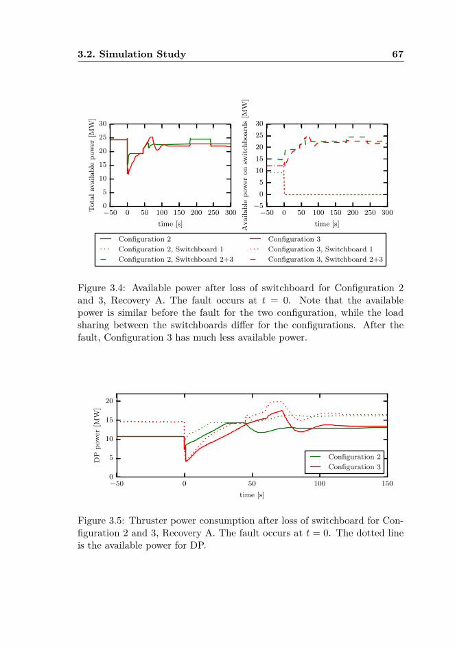
3.2. Simulation Study 67
−50 0 50 100 150 200 250 300
time [s]
0
5
10
15
20
25
30
Tota
lavail
ab
lep
ow
er[M
W]
−50 0 50 100 150 200 250 300
time [s]
−5
0
5
10
15
20
25
30
Avail
ab
lep
ow
eron
swit
chb
oard
s[M
W]
Configuration 2
Configuration 2, Switchboard 1
Configuration 2, Switchboard 2+3
Configuration 3
Configuration 3, Switchboard 1
Configuration 3, Switchboard 2+3
Figure 3.4: Available power after loss of switchboard for Configuration 2and 3, Recovery A. The fault occurs at t = 0. Note that the availablepower is similar before the fault for the two configuration, while the loadsharing between the switchboards differ for the configurations. After thefault, Configuration 3 has much less available power.
−50 0 50 100 150
time [s]
0
5
10
15
20
DP
pow
er[M
W]
Configuration 2
Configuration 3
Figure 3.5: Thruster power consumption after loss of switchboard for Con-figuration 2 and 3, Recovery A. The fault occurs at t = 0. The dotted lineis the available power for DP.
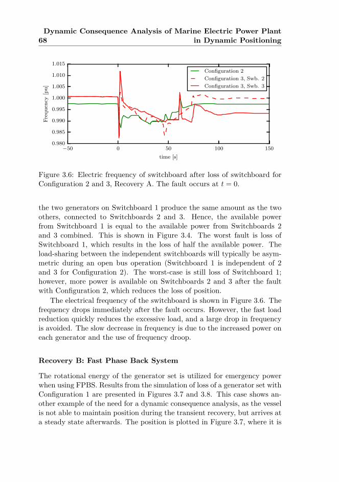
68Dynamic Consequence Analysis of Marine Electric Power Plant
in Dynamic Positioning
−50 0 50 100 150
time [s]
0.980
0.985
0.990
0.995
1.000
1.005
1.010
1.015
Fre
qu
ency
[pu
]
Configuration 2
Configuration 3, Swb. 2
Configuration 3, Swb. 3
Figure 3.6: Electric frequency of switchboard after loss of switchboard forConfiguration 2 and 3, Recovery A. The fault occurs at t = 0.
the two generators on Switchboard 1 produce the same amount as the twoothers, connected to Switchboards 2 and 3. Hence, the available powerfrom Switchboard 1 is equal to the available power from Switchboards 2and 3 combined. This is shown in Figure 3.4. The worst fault is loss ofSwitchboard 1, which results in the loss of half the available power. Theload-sharing between the independent switchboards will typically be asym-metric during an open bus operation (Switchboard 1 is independent of 2and 3 for Configuration 2). The worst-case is still loss of Switchboard 1;however, more power is available on Switchboards 2 and 3 after the faultwith Configuration 2, which reduces the loss of position.
The electrical frequency of the switchboard is shown in Figure 3.6. Thefrequency drops immediately after the fault occurs. However, the fast loadreduction quickly reduces the excessive load, and a large drop in frequencyis avoided. The slow decrease in frequency is due to the increased power oneach generator and the use of frequency droop.
Recovery B: Fast Phase Back System
The rotational energy of the generator set is utilized for emergency powerwhen using FPBS. Results from the simulation of loss of a generator set withConfiguration 1 are presented in Figures 3.7 and 3.8. This case shows an-other example of the need for a dynamic consequence analysis, as the vesselis not able to maintain position during the transient recovery, but arrives ata steady state afterwards. The position is plotted in Figure 3.7, where it is
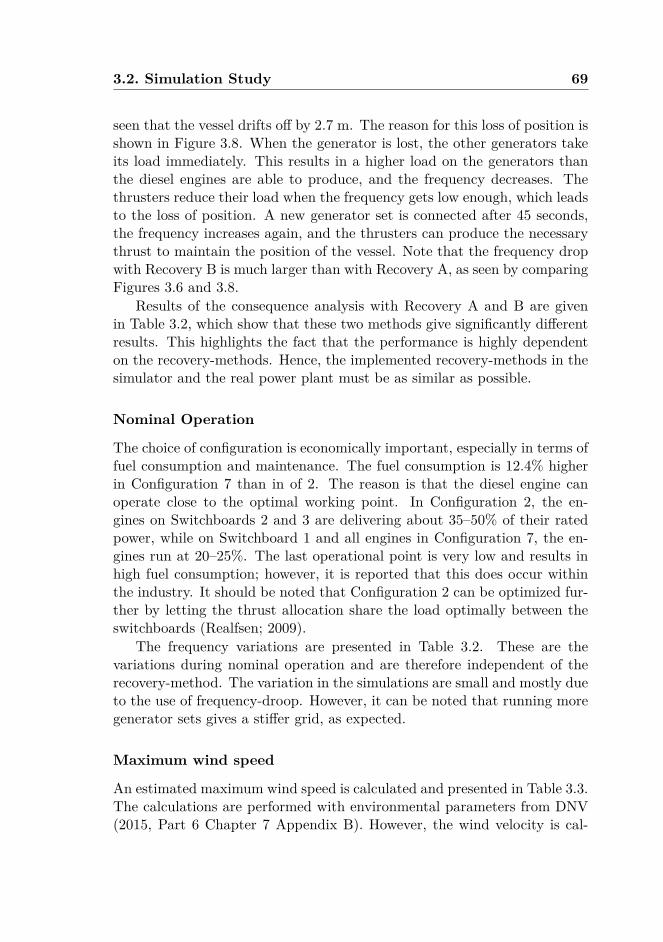
3.2. Simulation Study 69
seen that the vessel drifts off by 2.7 m. The reason for this loss of position isshown in Figure 3.8. When the generator is lost, the other generators takeits load immediately. This results in a higher load on the generators thanthe diesel engines are able to produce, and the frequency decreases. Thethrusters reduce their load when the frequency gets low enough, which leadsto the loss of position. A new generator set is connected after 45 seconds,the frequency increases again, and the thrusters can produce the necessarythrust to maintain the position of the vessel. Note that the frequency dropwith Recovery B is much larger than with Recovery A, as seen by comparingFigures 3.6 and 3.8.
Results of the consequence analysis with Recovery A and B are givenin Table 3.2, which show that these two methods give significantly differentresults. This highlights the fact that the performance is highly dependenton the recovery-methods. Hence, the implemented recovery-methods in thesimulator and the real power plant must be as similar as possible.
Nominal Operation
The choice of configuration is economically important, especially in terms offuel consumption and maintenance. The fuel consumption is 12.4% higherin Configuration 7 than in of 2. The reason is that the diesel engine canoperate close to the optimal working point. In Configuration 2, the en-gines on Switchboards 2 and 3 are delivering about 35–50% of their ratedpower, while on Switchboard 1 and all engines in Configuration 7, the en-gines run at 20–25%. The last operational point is very low and results inhigh fuel consumption; however, it is reported that this does occur withinthe industry. It should be noted that Configuration 2 can be optimized fur-ther by letting the thrust allocation share the load optimally between theswitchboards (Realfsen; 2009).
The frequency variations are presented in Table 3.2. These are thevariations during nominal operation and are therefore independent of therecovery-method. The variation in the simulations are small and mostly dueto the use of frequency-droop. However, it can be noted that running moregenerator sets gives a stiffer grid, as expected.
Maximum wind speed
An estimated maximum wind speed is calculated and presented in Table 3.3.The calculations are performed with environmental parameters from DNV(2015, Part 6 Chapter 7 Appendix B). However, the wind velocity is cal-
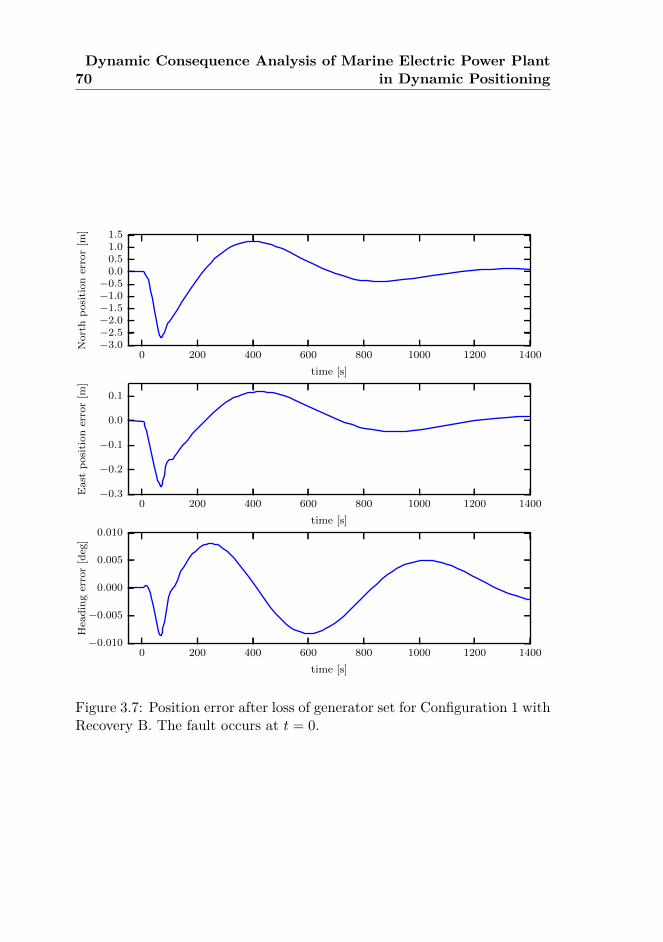
70Dynamic Consequence Analysis of Marine Electric Power Plant
in Dynamic Positioning
0 200 400 600 800 1000 1200 1400
time [s]
−3.0−2.5−2.0−1.5−1.0−0.5
0.00.51.01.5
Nort
hp
osi
tion
erro
r[m
]
0 200 400 600 800 1000 1200 1400
time [s]
−0.3
−0.2
−0.1
0.0
0.1
East
posi
tion
erro
r[m
]
0 200 400 600 800 1000 1200 1400
time [s]
−0.010
−0.005
0.000
0.005
0.010
Hea
din
ger
ror
[deg
]
Figure 3.7: Position error after loss of generator set for Configuration 1 withRecovery B. The fault occurs at t = 0.
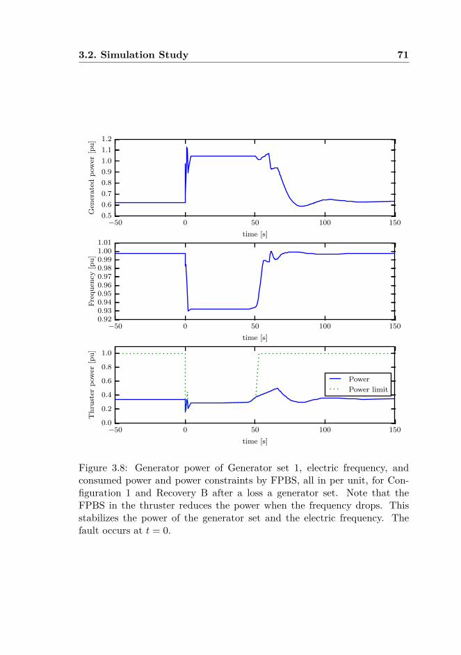
3.2. Simulation Study 71
−50 0 50 100 150
time [s]
0.5
0.6
0.7
0.8
0.9
1.0
1.1
1.2
Gen
erate
dp
ow
er[p
u]
−50 0 50 100 150
time [s]
0.920.930.940.950.960.970.980.991.001.01
Fre
qu
ency
[pu
]
−50 0 50 100 150
time [s]
0.0
0.2
0.4
0.6
0.8
1.0
Th
rust
erp
ow
er[p
u]
Power
Power limit
Figure 3.8: Generator power of Generator set 1, electric frequency, andconsumed power and power constraints by FPBS, all in per unit, for Con-figuration 1 and Recovery B after a loss a generator set. Note that theFPBS in the thruster reduces the power when the frequency drops. Thisstabilizes the power of the generator set and the electric frequency. Thefault occurs at t = 0.
72Dynamic Consequence Analysis of Marine Electric Power Plant
in Dynamic Positioning
Table 3.3: Maximum wind speed for different configurations and Recov-ery A.
Configuration 1 2 3 4 5 6 7Maximum windspeed [m/s]
2.19 10.01 7.48 10.01 6.21 10.01 10.01
culated without any safety-margin and is only valid for the 10 heading.The accepted wind velocity is underestimated, since only values given fromthe environmental regularity-numbers in DNV (2015, Part 6 Chapter 7 Ap-pendix B) were tested. For example, the velocities 10.01 and 11.39 m/s weretested for Configuration 2, and the fault scenarios passed for 10.01 m/s, butnot for 11.39 m/s. Therefore, the configuration’s maximum allowed windvelocity is between 10.01 m/s and 11.39 m/s.
DP-capability plot
A DP-capability plot is shown in Figure 3.9. It is calculated, for vary-ing headings, both with the standard static method, see for example DNV(2015, Part 6 Chapter 7 Appendix B), and with the method presented inthis chapter. In this case no safety-margins are used for either method. Thepresented method gives a conservative estimate compared with the staticmethod, since it includes both the transient recovery and the power con-straint.
3.2.3 Discussion
The results from this case study show that a vessel may be able to withstandthe mean environmental forces after a fault, but during the transient faultrecovery the vessel may temporarily lose position. It is also shown thatdifferent fault recovery-methods result in significantly different responses ofthe power plant and the vessel. Therefore, the consequence analysis can beused to choose the configuration of the power system and recovery functions.
The safety-factor in this simulation study is chosen as 1.1, as an exam-ple. Since the wave-drift forces are proportional to the square of the waveheight, the force increased by 21% from the nominal to the fault scenario.Similar consideration can be made for both current and wind forces, as theyare proportional to the square of the velocity. This approach is conservative,because it assumes that the power plant’s worst fault event coincides with
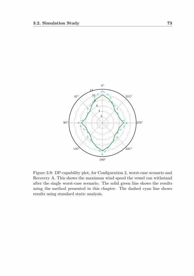
3.2. Simulation Study 73
0
45
90
135
180
225
270
315
2
4
6
8
10
12
Figure 3.9: DP-capability plot, for Configuration 2, worst-case scenario andRecovery A. This shows the maximum wind speed the vessel can withstandafter the single worst-case scenario. The solid green line shows the resultsusing the method presented in this chapter. The dashed cyan line showsresults using standard static analysis.
74Dynamic Consequence Analysis of Marine Electric Power Plant
in Dynamic Positioning
the worst-case waves, current, wind, and power consumption. Another ap-proach may be to give a probability-threshold then calculate a safety-factor.However, this is outside the scope of this chapter. It should be noted thatthe safety-factor can be changed with the operation. A high factor can beused during critical operations, such as diving and drilling, while a lowerfactor can be used during non-critical operations, such as standby.
The simulation cases consider a vessel with AC switchboards; however,more and more vessels are now equipped with DC switchboards and bat-teries for emergency power (Hansen and Wendt; 2015). This consequenceanalysis is well suited to these types of vessel, as a dynamic model is ableto verify the transient performance of such vessels. The method can alsobe used to check that the batteries have sufficient power and energy capac-ity to recover the power plant and terminate the operation, as required byDNV GL (2015b, Pt. 6 Ch. 3 Sec. 1 4.3.1). A simulation-based approachmay be needed as batteries may get warm during high power demands, andin such cases the batteries may disconnect due to safety protection systems.
The switchboard voltage will be low during a short circuit of the equip-ment connected to the switchboard. Hence, equipment with low voltageprotection may disconnect. The simulator is not able to simulate such fasttransients of the electric system. Therefore, fault ride through capability ofthe essential equipment should be verified by other methods to avoid thatequipment being disconnected or damaged during the recovery of the powerplant.
Not only is the configuration of the switchboard important, the param-eter settings of some functions, such as load sharing, load shedding, andthrust allocation, are also important. Optimization of these parameters isnecessary to obtain optimal power plant operation. However, care should betaken when optimizing with respect to only a few scenarios. In such cases theoptimum will sometimes result in changing the worst-case scenario from onescenario to another. For example, if the optimized worst-case is a blackoutof Switchboard 1, the optimum may be to increase the load on the otherswitchboards and let Switchboard 1 produce no load. This changes theworst-case from blackout of Switchboard 1, to blackout of one of the otherswitchboards. Therefore, individual blackout scenarios for each switchboardmust be included and not only those for the most critical switchboard. Opti-mizing the parameters is also a much more computationally expensive task,since many values of the continuous parameters must be checked to find theoptimum.
The simulation study in Pivano et al. (2014) considers stationkeeping
3.3. Conclusion 75
performance after the transient fault recovery was complete. They did showthat the vessel may not be able to maintain its position even though thevessel had sufficiently available thrust for the mean force. The method inthis chapter cannot detect such performance issues as only the low-frequencymotion is simulated. Therefore, a combination of the transient simulationin this chapter and the “steady-state” wave-frequency simulation in Pivanoet al. (2014) is necessary.
As noted in DNV GL (2015a), more analysis is necessary to verify theintegrity of a power system. Such dynamic analysis may include selectivity,short-circuits, and earth fault analysis. It is also assumed that each switch-board is independent of the others, and this must be verified (e.g., with anFMEA).
Reactive power is not considered in this simulation study; however, agenerator set can trip due to reactive power overload. Consequently, loadreduction and fault analysis with regard to reactive power should be con-sidered.
During simulations, not shown in this chapter, the transient loss of posi-tion after a fault was seldom a problem for cases when the standby generatorsets were not accounted for in the consequence analysis.
3.3 ConclusionA dynamic consequence analysis tool based on time-domain simulation isshown in this study. Different configurations were simulated during multiplefault scenarios to evaluate the DP-performance during transient recovery.It is observed for the chosen cases that the transient recoveries after faultsare the limiting factor when choosing a configuration, as the vessel maybe able to maintain its position before and after the fault, but not duringthe transition. This is especially important for configurations where one ormore standby generators are connected after a fault, as recently allowed bysome class notations. It is seen that the result of a reconfiguration can beunpredictable as the thruster system and power plant are complex systems.This method allows the power plant to be configured depending on therequired safety level, since more safety-margins can be used during criticaland non-critical operations.

76Dynamic Consequence Analysis of Marine Electric Power Plant
in Dynamic Positioning
Chapter 4
Dynamic Safety Constraintsby Scenario-Based EconomicModel Predictive Control
This chapter is based on Bø and Johansen (2014, n.d.b).
4.1 IntroductionThere is a need for autonomous handling of faults in many industrial controlsystems. These faults can be due to actuator faults, sensor faults, externalfaults, or internal faults. There are also often constraints on the system tomake sure that the system is safe. However, it can take some time beforethe controller is fully reconfigured and the system recovers after a fault.Conservative safety limits are therefore sometimes used to make sure thatthe system is safe also during the transients after the fault.
Active redundancy is often used when downtime of a system is not ac-ceptable. This is the case for the electrical power system on board ad-vanced marine vessels. A typical marine power plant consists of multiplepairs of generators and diesel engines. The generators are connected toswitchboards which distribute the electrical power to thrusters and otherconsumers. However, sudden disconnection of generators does happen, andthen the load from the disconnected generator is shared among the remain-ing generators. The electric frequency will then decrease due to slow dy-namics in the diesel engine. Therefore, a safety margin is needed to avoidunder-frequency protection trip after disconnection of a generator. This istypically handled by regulating a fixed frequency and reducing the loads
77
78Dynamic Safety Constraints by Scenario-Based Economic Model
Predictive Control
when a fault occurs. However, the controller has more freedom for opti-mization if the frequency is allowed to vary within some dynamic safetyconstraints and unnecessary load reduction can be avoided. Therefore, theplant can be safer and increase the operational performance by explicitlyincluding the fault scenarios in the controller. Detecting that the systemcannot recover from a fault is as important as recovering the system. Wetherefore propose a method for detecting if the faults can or cannot be re-covered from. Such information can be used for proactive reconfigurationof the plant, or change of control objective.
Model predictive control (MPC) with scenarios will be used to establisha fault-tolerant controller. Scenarios in MPCs are mostly used for robustMPC. An MPC for linear systems is presented in Bernardini and Bemporad(2009), where the system matrices can switch between a finite number ofscenarios, with a given probability for each scenario. Other combinationsof MPC and scenarios are presented in e.g., Calafiore and Fagiano (2013);Maiworm et al. (2015); Schildbach et al. (2014). These studies use scenariosto handle model uncertainties and disturbances. It has been proposed touse approximate reachable sets to establish a robust MPC (Bravo et al.;2006). However, this gives conservative estimates, since a common controlinput is calculated for all possible sequences of uncertainties and distur-bances (open-loop control). For linear systems, Scokaert and Mayne (1998)suggest including feedback in the optimization problem. For non-linear sys-tems this gives an infinite dimension optimization problem, it is thereforeproposed to use a semi-feedback formulation, see Limon et al. (2009) and thereferences therein. Scenario-based model predictive control has also beensuggested used in optimization of hedge options (Bemporad et al.; 2014),for scheduling of batch processes (Bonfill et al.; 2008), and scheduling ofemergency vehicles (Goodwin and Medioli; 2013).
There have been some studies on transients of the plant after reconfig-uration of controllers due to faults. An investigation of responses due toreconfiguration of the controller is presented in Kovâcshâzy et al. (2001),with different method for initializing the next controller. For faults whichcan be predicted, it has been suggests to use MPC to make a smooth ac-commodation of the fault (Lao et al.; 2013). It is suggested to use backcalculation to set the initial states of the reconfigured controller and usea progressive accommodation scheme to achieve new LQR-gains (Blankeet al.; 2006).
Another approach to control a plant to a safe set is to use backwardreachable set to calculate the fault-tolerant set (Gillula et al.; 2011). The
4.2. Problem Statement 79
backward reachable set is a set containing all initial states which can avoidan unsafe state set, under a specified set of disturbances. A method for vali-dating that a controller can avoid unsafe sets for linear hybrid systems usingreachability analysis is presented in Torrisi and Bemporad (2001). A similarstudy is done for nonlinear hybrid system using barrier certificates (Prajnaet al.; 2007). A method for selecting switching rules for a hybrid system,such that the state variables avoid an unsafe set, is presented in Cooganand Arcak (2012).
The method presented in the present chapter is a variant of the methodpresented in Bernardini and Bemporad (2009). However, in the presentchapter the models are nonlinear, fault-tolerance and economic objectiveemphasized, and a deterministic framework is used.
Control of the speed of generator sets in a marine diesel-electric powerplant are one of the example cases in the present chapter. Currently gener-ator sets are controlled in speed droop or isochronous using PID or similaralgorithms for speed governors (Ådnanes; 2003). Model predictive controland nonlinear control by feedback linearization are proposed as alternativecontrol methods (Hansen et al.; 1998; Hansen and Fossen; 1999; Veksleret al.; 2013). In Radan (2008), multiple methods for better control of en-gines are proposed, this includes observer design, for noise-filtering, andinertia control, to suppress frequency variations.
The present chapter presents a method for establishing dynamic safetyconstraints based on fault scenario. The idea of the controller was firstpresented in Bø and Johansen (2013), for a marine electric power plant.It was later formalized in Bø and Johansen (2014), including a linear caseplant. The MPC uses multiple predictions internally for each fault sce-nario in addition to the nominal scenario. By using this method the safetyconstraints are moved from being applied to the nominal scenario to beingapplied to the fault scenario, and this is the main contribution of this chap-ter. Therefore, this method is suited when the constraints are set to avoidunsafe states, e.g., during the transients after a fault. Typically, this givesless conservative constraints and the opportunity to operate the plant saferwith increased performance. The controller is applied to two example cases,a linear plant and a marine electric power plant.
4.2 Problem Statement
Consider a plant where we have safety constraints on the control input andthe states. In particular, there are given some fault scenarios which the
80Dynamic Safety Constraints by Scenario-Based Economic Model
Predictive Control
plant must be able to handle safely. We would like to design a controllerwhich makes sure that the plant can be recovered after any of these faultscenarios. This consists of three requirements:
Recoverability: The controller should keep the system in a state set whereit is possible to recover the system if one of the fault scenarios occurs.
Robust Control: The controller should use a control input which is ap-propriate for the nominal system and the faulty system until the faultis detected and the fault is accommodated by the controller.
Detection of recoverability: It should be detected if the system cannotbe recovered when one of the fault scenarios occurs.
The fault scenarios considered in this chapter are modeled as change ofthe dynamics or constraints of the system.
4.3 Model DescriptionThe plant is described with one model for each scenario. The differenceequation for the states is of the form:
x(tk+1) = f(x(tk),u(tk)) (4.1)
where x ∈ Rn and u ∈ Rm are the state and input vectors. The state andcontrol input vectors for the control horizon are given by:
X(ti) =[x>(ti) . . . x>(ti+N−1)
]>(4.2)
U(ti) =[u>(ti) . . . u>(ti+N−1)
]>(4.3)
where ti is the time instant at the beginning of the control horizon, andN denotes the length of the control horizon. Note that we assume no un-known disturbances, model uncertainties, or measurement noise; however,these effects can be included as additional scenarios along with faults, or bytightening the constraints. The state and control input are constrained by:
Gnr(x,u) ≤ 0Gr(x,u) ≤ s0 ≤ s
(4.4)
where Gnr(x,u) : Rn × Rm → Rncn and Gr(x,u) : Rn × Rm → Rncr . It isassumed that all non-relaxable constraints (hard constraints) are stacked in
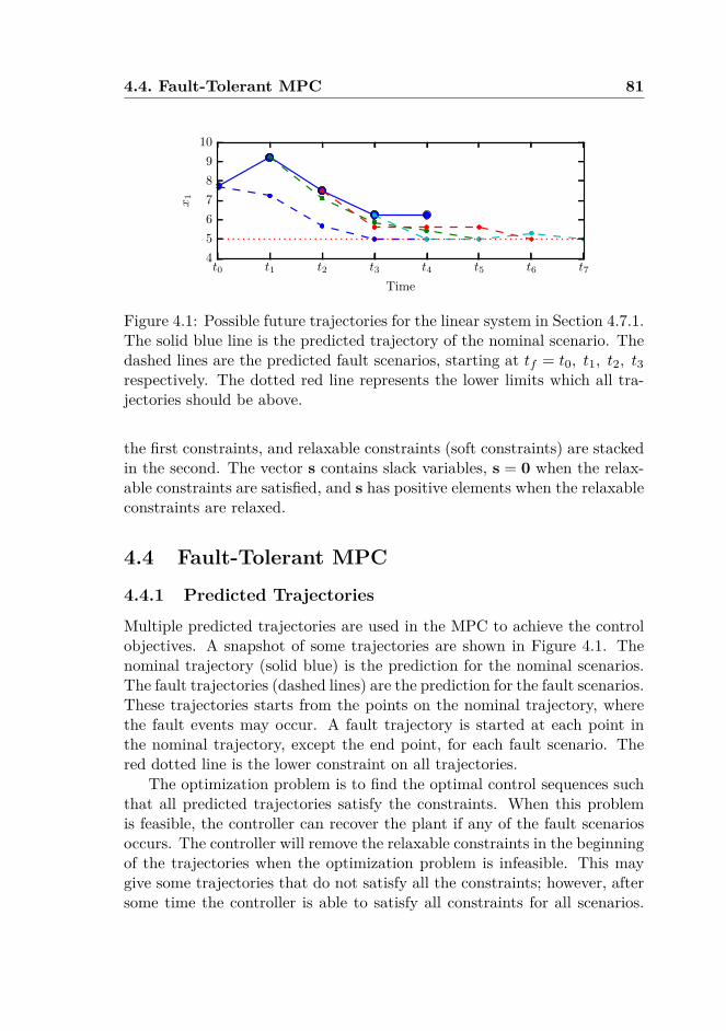
4.4. Fault-Tolerant MPC 81
t0 t1 t2 t3 t4 t5 t6 t7
Time
4
5
6
7
8
9
10
x1
Figure 4.1: Possible future trajectories for the linear system in Section 4.7.1.The solid blue line is the predicted trajectory of the nominal scenario. Thedashed lines are the predicted fault scenarios, starting at tf = t0, t1, t2, t3respectively. The dotted red line represents the lower limits which all tra-jectories should be above.
the first constraints, and relaxable constraints (soft constraints) are stackedin the second. The vector s contains slack variables, s = 0 when the relax-able constraints are satisfied, and s has positive elements when the relaxableconstraints are relaxed.
4.4 Fault-Tolerant MPC
4.4.1 Predicted Trajectories
Multiple predicted trajectories are used in the MPC to achieve the controlobjectives. A snapshot of some trajectories are shown in Figure 4.1. Thenominal trajectory (solid blue) is the prediction for the nominal scenarios.The fault trajectories (dashed lines) are the prediction for the fault scenarios.These trajectories starts from the points on the nominal trajectory, wherethe fault events may occur. A fault trajectory is started at each point inthe nominal trajectory, except the end point, for each fault scenario. Thered dotted line is the lower constraint on all trajectories.
The optimization problem is to find the optimal control sequences suchthat all predicted trajectories satisfy the constraints. When this problemis feasible, the controller can recover the plant if any of the fault scenariosoccurs. The controller will remove the relaxable constraints in the beginningof the trajectories when the optimization problem is infeasible. This maygive some trajectories that do not satisfy all the constraints; however, aftersome time the controller is able to satisfy all constraints for all scenarios.
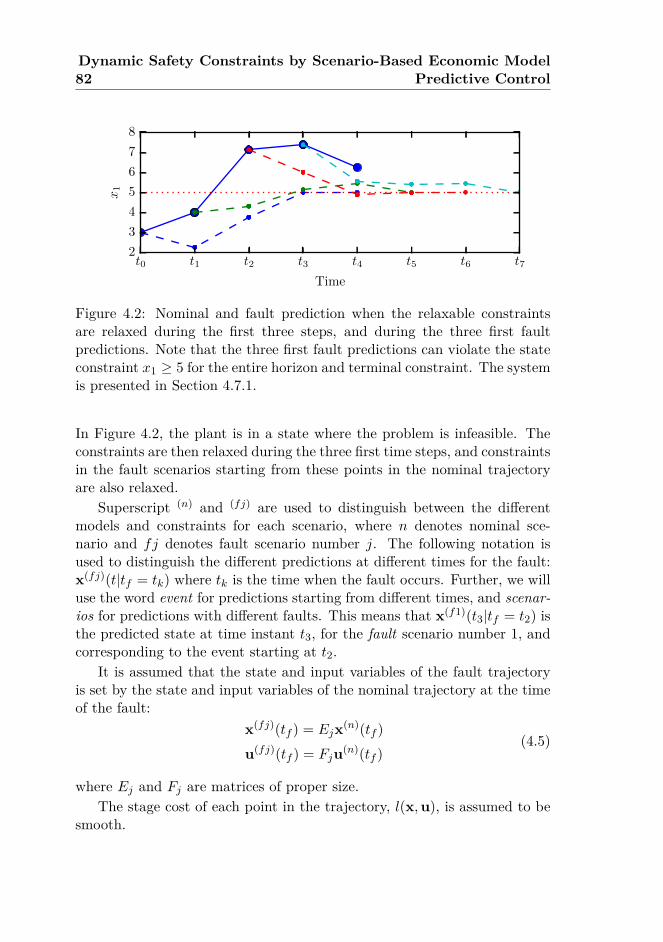
82Dynamic Safety Constraints by Scenario-Based Economic Model
Predictive Control
t0 t1 t2 t3 t4 t5 t6 t7
Time
2
3
4
5
6
7
8
x1
Figure 4.2: Nominal and fault prediction when the relaxable constraintsare relaxed during the first three steps, and during the three first faultpredictions. Note that the three first fault predictions can violate the stateconstraint x1 ≥ 5 for the entire horizon and terminal constraint. The systemis presented in Section 4.7.1.
In Figure 4.2, the plant is in a state where the problem is infeasible. Theconstraints are then relaxed during the three first time steps, and constraintsin the fault scenarios starting from these points in the nominal trajectoryare also relaxed.
Superscript (n) and (fj) are used to distinguish between the differentmodels and constraints for each scenario, where n denotes nominal sce-nario and fj denotes fault scenario number j. The following notation isused to distinguish the different predictions at different times for the fault:x(fj)(t|tf = tk) where tk is the time when the fault occurs. Further, we willuse the word event for predictions starting from different times, and scenar-ios for predictions with different faults. This means that x(f1)(t3|tf = t2) isthe predicted state at time instant t3, for the fault scenario number 1, andcorresponding to the event starting at t2.
It is assumed that the state and input variables of the fault trajectoryis set by the state and input variables of the nominal trajectory at the timeof the fault:
x(fj)(tf ) = Ejx(n)(tf )u(fj)(tf ) = Fju(n)(tf )
(4.5)
where Ej and Fj are matrices of proper size.The stage cost of each point in the trajectory, l(x,u), is assumed to be
smooth.
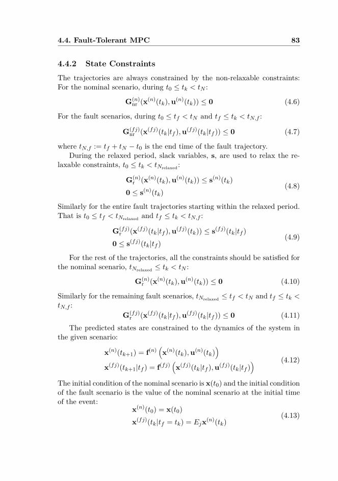
4.4. Fault-Tolerant MPC 83
4.4.2 State Constraints
The trajectories are always constrained by the non-relaxable constraints:For the nominal scenario, during t0 ≤ tk < tN :
G(n)nr (x(n)(tk),u(n)(tk)) ≤ 0 (4.6)
For the fault scenarios, during t0 ≤ tf < tN and tf ≤ tk < tN,f :
G(fj)nr (x(fj)(tk|tf ),u(fj)(tk|tf )) ≤ 0 (4.7)
where tN,f := tf + tN − t0 is the end time of the fault trajectory.During the relaxed period, slack variables, s, are used to relax the re-
laxable constraints, t0 ≤ tk < tNrelaxed :
G(n)r (x(n)(tk),u(n)(tk)) ≤ s(n)(tk)
0 ≤ s(n)(tk)(4.8)
Similarly for the entire fault trajectories starting within the relaxed period.That is t0 ≤ tf < tNrelaxed and tf ≤ tk < tN,f :
G(fj)r (x(fj)(tk|tf ),u(fj)(tk)) ≤ s(fj)(tk|tf )
0 ≤ s(fj)(tk|tf )(4.9)
For the rest of the trajectories, all the constraints should be satisfied forthe nominal scenario, tNrelaxed ≤ tk < tN :
G(n)r (x(n)(tk),u(n)(tk)) ≤ 0 (4.10)
Similarly for the remaining fault scenarios, tNrelaxed ≤ tf < tN and tf ≤ tk <tN,f :
G(fj)r (x(fj)(tk|tf ),u(fj)(tk|tf )) ≤ 0 (4.11)
The predicted states are constrained to the dynamics of the system inthe given scenario:
x(n)(tk+1) = f(n)(x(n)(tk),u(n)(tk)
)x(fj)(tk+1|tf ) = f(fj)
(x(fj)(tk|tf ),u(fj)(tk|tf )
) (4.12)
The initial condition of the nominal scenario is x(t0) and the initial conditionof the fault scenario is the value of the nominal scenario at the initial timeof the event:
x(n)(t0) = x(t0)x(fj)(tk|tf = tk) = Ejx(n)(tk)
(4.13)
84Dynamic Safety Constraints by Scenario-Based Economic Model
Predictive Control
4.4.3 Robust Control Input
Fault detection, identification, and fault accommodation will often takesome time. It is therefore important that the control input is appropri-ate in the time between the fault occurs and the fault is accommodatedin the controller. The fault trajectories are therefore restricted to use thesame control input as the nominal trajectory during the first time stepsof the fault trajectory. We define τrobust as the maximum number of timeunits between a fault occur and the controller is reconfigured. This givesthe following additional constraints, for k ≤ i < min(k + τrobust, N):
u(fj)(ti|tf = tk) = Fju(n) (4.14)
For tf + τrobust ≥ tN the inputs are constrained to be equal to u(n)s, sincewe can prolong the nominal trajectory with the pairs (x(n)s,u(n)s):
u(fj)(ti|tf = tk) = Fju(n)s (4.15)
where x(n)s and u(n)s are later defined in Definition 2.
4.4.4 Terminal Constraints
Terminal constraints are used to achieve recursive feasibility. This is doneby finding the optimal equilibrium of each scenario and constraining theend of the predicted state trajectories to this state.
Remark 1 In the MPC literature it is known that equilibrium terminalconstraints often lead to numerical challenges and may suffer from smallregion of attraction. For this reason a terminal set constraint rather thana terminal point constraint has benefits. However, for the case plants inSection 4.7, the constraints are active and the stage cost may be non-zeroon the optimal safe equilibrium (defined later in this section). For suchsystem, the authors are only aware of results on recursive feasibility whenterminal equilibrium constraint is used (Angeli et al.; 2012). One exceptionis Grüne (2013), but this approach requires other strong assumptions.
The fault trajectories are constrained by the optimal equilibrium termi-nal constraints. It is defined as:
Definition 1 An optimal equilibrium for fault scenario j, (x(fj)o,u(fj)o) is
4.4. Fault-Tolerant MPC 85
any solution to:
(x(fj)o,u(fj)o) = arg minx(fj),u(fj)
l(fj)(x(fj),u(fj))
such thatx(fj) = f(fj)(x(fj),u(fj))G(fj)
r (x(fj),u(fj)) ≤ 0G(fj)
nr (x(fj),u(fj)) ≤ 0
(4.16)
The optimal steady state cost is l(fj)o = l(fj)(x(fj)o,u(fj)o).
For convenience we assume an optimal equilibrium exists and is unique.The terminal value of the non-relaxed fault trajectories is constrained
to the optimal equilibrium:
x(fj)(tN,f |tf ) = x(fj)o (4.17)
The constraint is relaxed for t0 ≤ tf < tNrelaxed :
x(fj)(tN,f |tf ) = x(fj)o − s−(fj)N (tf ) + s+(fj)
N (tf )
0 ≤ s−(fj)N (tf )
0 ≤ s+(fj)N (tf )
(4.18)
where s−N and s+N are slack variables and x(fj)o is found by solving (4.16).
A terminal stability constraint is used for the nominal scenario, both tomake sure that the limit of the closed loop average cost is upper boundedand to make sure that the control problem is recursively feasible. We startby defining an optimal safe equilibrium.
Definition 2 An optimal safe equilibrium for the nominal scenario, (x(n)s,u(n)s),is any solution to:
(x(n)s,u(n)s) = arg minx(n),u(n)
l(n)(x(n),u(n))
such that(x(n),u(n)) ∈ Zsafe,eq
G(n)r (x(n),u(n)) ≤ 0
G(n)nr (x(n),u(n)) ≤ 0
(4.19)
86Dynamic Safety Constraints by Scenario-Based Economic Model
Predictive Control
where Zsafe,eq is the set of equilibrium points satisfying x(n) = f(n)(x(n),u(n))such that for each fault scenario j there exist a feasible trajectory with thelength N :
• starting at Ejx(n),
• the control input of the fault scenario is Fju(n) during the first τrobustsamples of the trajectory,
• the constraints (4.7) and (4.11) are satisfied at every point on thetrajectory and (4.17) at the end point of the trajectory.
The optimal safe equilibrium cost is l(n)s = l(n)(x(n)s,u(n)s).
For convenience we assume that there exists an unique optimal safeequilibrium. The terminal constraint for the nominal trajectory is:
x(n)(tN ) = x(n)s (4.20)
where x(n)s is found by solving (4.19).
4.4.5 Optimization Problem
All optimization variables can be stacked in a vector U , containing con-trol inputs and slack variables for all scenarios. Penalty functions gi(s)and gN (s+, s−) are added to the cost function to limit the violation of theconstraints. The objective function is:
φ(x(t0),U) =N−1∑i=0
l(x(n)(ti),u(n)(ti))
+N−1∑i=0
g(n)i (s(n)(ti))
+M∑
j=1
N−1∑i=0
w(fj)i
[N−1∑k=0
g(fj)k (s(fj)(tk|tf = ti))
+ g(fj)N (s−(fj)(tf = ti), s+(fj)(tf = ti))
](4.21)
where the first term is the sum of the stage costs of the nominal scenario,the second term is the penalty cost of the nominal trajectory, and the lastterm is the penalty of the fault scenarios. M is the number of fault scenarios
4.4. Fault-Tolerant MPC 87
and w(fj)i are positive weights for fault scenario j. For example, the con-
troller may optimize the input for feasibility of the most probable scenarioby using the probability of each scenario as weights. Other choices can beto use the risk of each scenario or a priority of scenarios. Note that thestage costs of the fault scenarios are not included, since we often only wantthe fault scenarios to be feasible and it is not important that their trajec-tories are optimal. We assume all functions (models, cost, and constraints)are smooth, so that the optimization problem is well defined with globalsolutions.
A minimal time approach will be used to make sure that the plant getssafe as quickly as possible (Rawlings and Muske; 1993). This means thatbefore solving for the optimal trajectory we solve this problem:
(N∗relaxed, U) = arg minNrelaxed,U
Nrelaxed
subject to(4.6) – (4.15), (4.17), (4.18), and (4.20)
(4.22)
This is the smallest Nrelaxed needed to make the optimization problem fea-sible. Then, the optimal control sequence is found by solving:
U∗ = arg minU
φ(x(t0),U)
subject toNrelaxed = N∗relaxed
(4.6) – (4.15), (4.17), (4.18), and (4.20)
(4.23)
The controller will then apply κ(x(t0)) = u(n)∗(t0) from U∗, and in thenominal scenario the closed loop system is:
x(n)(tk+1) = f(n)(x(n)(tk), κ(n)(x(n)(tk)) (4.24)
The algorithm can be summarized in one offline step and two onlinesteps:
Offline: Find the optimal equilibrium for the fault scenarios and the opti-mal safe equilibrium for the nominal scenario by solving (4.16) and (4.19).
1. Online: Find N∗relaxed by solving (4.22).
2. Online: Find the optimal control sequence by solving (4.23).
88Dynamic Safety Constraints by Scenario-Based Economic Model
Predictive Control
Challenges related to the computation of global solution of nonlinearprograms in real time are well known and important. However, they areconsidered out of scope of this study.
Remark 2 Vada et al. (2001) have shown that for linear systems withquadratic cost, a linear penalty function can be designed to ensure that theproblem is feasible as early as possible in the prediction horizon. Hence, theonline steps can be merged into one step by using such penalty function.
4.5 Feasibility and StabilityTo investigate the stability of the fault tolerant MPC we first present anequivalent optimization problem. We will utilize the fact that there exista time-invariant set which can be used as a fixed constraint set, since thescenarios and system are time-invariant.
Definition 3 The safe state set, Xsafe, is the largest forward invariant setcontaining all x(t0) such that the optimization problem (4.23) is feasible withzero slack variables (i.e., s = 0). Let XN denote the set where there exist asolution to (4.23) with horizon length N .
Lemma 1 Assuming the states have converged to Xsafe (i.e., Nrelaxed = 0)the optimization problem (4.23) can be simplified to the following:
U∗ = arg minU
N−1∑i=0
l(n)(x(n)(ti),u(n)(ti))
such thatx(n)(ti) ∈ Xsafe
x(n)(ti+1) = f(n)(x(n)(ti),u(n)(ti))
t0 ≤ ti < tN
x(n)(tN ) = x(n)s
(4.25)
This optimization problem gives the controller and the nominal closedloop system:
κ(n)l (x(n)(tk)) = u(n)∗(tk) (4.26)
x(tk+1)(n) = f(n)(x(n)(tk), κ(n)l (x(tk))) (4.27)
The optimal nominal trajectory of optimization problem (4.23) is alsothe optimal trajectory of (4.25).
4.5. Feasibility and Stability 89
Proof The optimization problem (4.23) can be reformulated to (4.25) bythe steps below. All constraints are satisfied in Xsafe, including the relaxableconstraints. Consequently, slack variables and penalty functions can beremoved. The fault scenarios does only make sure that x(n) ∈ Xsafe anddoes not alter the cost. Hence, they can be removed from the optimizationproblem when x(n) ∈ Xsafe and x(n) is constrained to be within Xsafe. Itfollows, that the optimal nominal trajectory of these equivalent optimizationproblems will be equal, since the optimization problems are equivalent.
Lemma 2 For all closed loop trajectories starting from x(n)(t0) ∈ Xsafe thetrajectory of the nominal system system (4.24) will not leave Xsafe and theaverage cost,
l = lim supN→∞
N∑k=0
l(x(tk), u(tk)N + 1 , (4.28)
will be lower or equal to the optimal safe steady state cost.
Proof This results follows directly from Theorem 1 in Angeli et al. (2012)by using the equivalent optimization problem (4.25).
Theorem 1 The following holds for the nominal scenario:
1. The optimization problem (4.23) will stay feasible if it is initially fea-sible.
2. It will take a maximum of N steps to reach Xsafe from the time (4.23)is feasible, and from that time it will stay in Xsafe.
3. The closed loop system has an average cost which is less than or equalto the optimal safe steady state cost for all initial conditions in XN .
Proof The recursive feasibility can be assured by a proof similar to Mayneet al. (2000). If we have a feasible input sequence at the previous step, we canalways shift this sequence one step and extended the tail with u(n)(tN−1) =u(n)s, denote this trajectory U′ and the corresponding state trajectory X′.This will make x(n)(tN ) = x(n)s ∈ Xsafe, and the nominal scenario feasible.We know that the shifted part of this trajectory will make all fault scenariosfeasible, since they were feasible at the previous step. For the prolonged part(x(n)(tN−1),u(n)(tN−1)
)=(x(n)s,u(n)s
), we know that this is not only
feasible, but it does also satisfy the relaxable and non-relaxable constraints.
90Dynamic Safety Constraints by Scenario-Based Economic Model
Predictive Control
Hence, this input sequence is feasible; therefore, the problem is recursivefeasible, and part (1) is proven.
Next, we prove that the closed loop system will enter Xsafe within Nsteps by induction. The trajectory U′ will make sure that the relaxableconstraints are feasible one time step earlier in the horizon than at theprevious iteration. We know that the solution will honor the constraintsas early as possible due to the minimization of Nrelaxed. The prediction ofx(tN ) ends up in Xsafe if the problem is feasible at t0. At each followingstep the length of the tail which honor the relaxable constraints is increasedwith at least one step. Therefore, it will not take longer than the length ofthe prediction horizon N to reach Xsafe. This proves result (2).
The third result follows from the fact that the states will reach Xsafe
in finite time. Further, from Lemma 2, we know that inside Xsafe the costis lower than or equal to l(n)s. Let tke be the time when the closed loopsystem enters Xsafe. The cost from t0 to tke is bounded, since l(·) is smoothon XN . The average cost will then be:
lim supN→∞
N∑i=0
l(x(ti),u(ti))N + 1
= lim supN→∞
ke∑i=0
l(x(ti),u(ti))N + 1 +
N∑i=ke
l(x(ti),u(ti))N + 1
= lim supN→∞
C1N + 1 +
N∑i=ke
l(x(ti),u(ti))N + 1
= lim supN→∞
N∑i=ke
l(x(ti),u(ti))N + 1 ≤ ls
(4.29)
Corollary 1 From the time x enters Xsafe the plant can be recovered fromany of the fault scenarios, without violating the constraints.
Proof This result follows directly from the definition of Xsafe and the factthat the state will stay in Xsafe after it has entered it.
4.6 Reconfigurable ControlThe controller may be reconfigured in the event that one of the fault sce-narios occurs. In this case, we are only interested in recovering the plant;
4.6. Reconfigurable Control 91
therefore, the MPC will only consider this fault. Slack variables are used torelax the constraints, since we cannot know in advance if the system is re-coverable (unless N∗relaxed = 0). The constraints during the relaxed period,t0 ≤ ti < tNrelaxed , are:
G(fj)r (x(fj)(ti),u(fj)(ti)) ≤ s(ti)
G(fj)nr (x(fj)(ti),u(fj)(ti)) ≤ 0
0 ≤ s(ti)(4.30)
and after the relaxed period, tNrelaxed ≤ ti < tN :
G(fj)r (x(fj)(ti),u(fj)(ti)) ≤ 0
G(fj)nr (x(fj)(ti),u(fj)(ti)) ≤ 0
(4.31)
The system is also constrained to the dynamics of the system:
x(fj)(ti+1) = f(fj)(x(fj)(ti),u(fj)(ti)) (4.32)
Terminal constraints are used to guarantee recursive feasibility:
x(fj)(tN ) = x(fj)o (4.33)
where x(fj)o is found by solving (4.16). To minimize the time before allconstraints are feasible, a minimal time approach will be used:
(N∗relaxed,U) = arg minNrelaxed,U
Nrelaxed
subject to (4.30)− (4.33)(4.34)
The optimal trajectory is found by solving the following optimization prob-lem:
U∗ = arg minU
N−1∑i=0
l(fj)(x(fj)(tk),u(fj)(tk)
)
+N−1∑k=0
g(fj)(s(fj)(tk))
subject to (4.30)− (4.33), Nrelaxed = N∗relaxed
(4.35)
which gives the control law and closed loop system:
κ(fj)(x(fj)(t0)) = u(fj)∗(t0) (4.36)x(fj)(tk+1) = f(fj)(x(tk), κ(fj)(x(tk))) (4.37)
92Dynamic Safety Constraints by Scenario-Based Economic Model
Predictive Control
Theorem 2 Assume fault scenario j occurs and the controller is switchedfrom κ(n) to κ(fj). Then the following holds for the fault scenario:
1. The optimization problem (4.35) will stay feasible if it is initially fea-sible.
2. It will take a maximum of N steps to make N∗relaxed = 0, and fromthat time it will be 0.
3. The average cost will be less than or equal to l(fj)o.
In addition, assume that the switch of controller is done within τrobust timeunits after the fault occurred and N∗relaxed = 0 at the time instant when thefault occurred. Then the following holds in addition for the fault scenario:
4. The optimization problem (4.35) is feasible with N∗relaxed = 0.
The proof is omitted, since it is similar to the proof of Theorem 1.
4.7 Case Study
4.7.1 Linear Plant with Nonlinear Cost
We present simulation results from a closed loop simulation of a linear plantwith nonlinear cost in this section. The discrete-time system equations are:
x(tk+1) =
1 5 50 1 00 0 1
x(tk) +
12.5 12.55 00 5
u(tk)−
100
b (4.38)
where x =[x1 x2 x3
]>is the states, u =
[u1 u2
]>is the control inputs,
and b is a known constant. The non-relaxable constraints (superscript isomitted as the constraints are valid for all scenarios):
0 ≤ x2 ≤ 1 −0.1 ≤ u1 ≤ 0.10 ≤ x3 ≤ 1 −0.1 ≤ u2 ≤ 0.1
(4.39)
The relaxable constraint is:
5 ≤ x1 (4.40)
This system can model a buffer tank with two slow pumps, where the pumpshave both saturation limits and rate constraints.
4.7. Case Study 93
The fault scenarios are that x2 or x3 is suddenly set to zero (e.g., afailure of one of two pumps). This gives:
x(f1)1 (tk+1) = x
(f1)1 (tk) + 5x(f1)
3 (tk) + 12.5u(f1)2 (tk)− b
x(f1)3 (tk+1) = x
(f1)3 (tk) + 5u(f1)
2 (tk)
x(f2)1 (tk+1) = x
(f2)1 (tk) + 5x(f2)
2 (tk) + 12.5u(f2)1 (tk)− b
x(f2)2 (tk+1) = x
(f2)2 (tk) + 5u(f2)
1 (tk)
(4.41)
The stage costs are:
l(n)(x(n)) = 10−4(x
(n)1
)4+(x
(n)2
)2+(x
(n)3
)2(4.42)
l(f1)(x(f1)) = 10−4(x
(f1)1
)4+(x
(f1)3
)2(4.43)
l(f2)(x(f2)) = 10−4(x
(f2)1
)4+(x
(f2)2
)2(4.44)
The penalty cost functions are (sub- and superscript is omitted as the func-tion is used for all scenarios and slack variables):
g(s) = (s− 100 · 1)2, (4.45)
for appropriate dimension of the vector 1.The controller is implemented in ACADO (Houska et al.; 2011), with
τrobust = 1. The constant b is set to 2.5, and the initial values are x1 = 10,x2 = 0.5, and x3 = 0. This gives the optimal safe equilibrium at x1 = 6.25,x2 = .25, x3 = .25, with the stage cost ls ≈ 0.2776. The horizon length is 4,which gives 40 optimization variables and 264 constraints. The computationtime is around 0.4 seconds per updating period. Results from closed-loopsimulation are shown in Figure 4.3, with and without fault. The total costof the fault free trajectory is 3.479.
A comparative controller with static constraints is designed to comparethe static safety constraint with scenario-based constraints. For this casewe let the safety constraints be:
x1 ≥ 8.75 (4.46)
This is the least conservative state constraint which ensure that the controlobjectives stated in Section 4.2 are fulfilled. The optimal equilibrium of thecontroller is x1 = 8.75 and x2 = x3 = 0.25, with the stage cost of 0.7112.In Figure 4.4, a similar simulation is shown as in Figure 4.3, but with
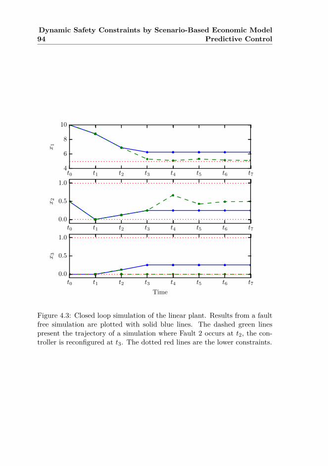
94Dynamic Safety Constraints by Scenario-Based Economic Model
Predictive Control
t0 t1 t2 t3 t4 t5 t6 t7
0.0
0.5
1.0
x2
t0 t1 t2 t3 t4 t5 t6 t74
6
8
10
x1
t0 t1 t2 t3 t4 t5 t6 t7
Time
0.0
0.5
1.0
x3
Figure 4.3: Closed loop simulation of the linear plant. Results from a faultfree simulation are plotted with solid blue lines. The dashed green linespresent the trajectory of a simulation where Fault 2 occurs at t2, the con-troller is reconfigured at t3. The dotted red lines are the lower constraints.
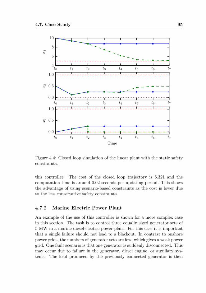
4.7. Case Study 95
t0 t1 t2 t3 t4 t5 t6 t7
0.0
0.5
1.0
x2
t0 t1 t2 t3 t4 t5 t6 t74
6
8
10
x1
t0 t1 t2 t3 t4 t5 t6 t7
Time
0.0
0.5
1.0
x3
Figure 4.4: Closed loop simulation of the linear plant with the static safetyconstraints.
this controller. The cost of the closed loop trajectory is 6.321 and thecomputation time is around 0.02 seconds per updating period. This showsthe advantage of using scenario-based constraints as the cost is lower dueto the less conservative safety constraints.
4.7.2 Marine Electric Power Plant
An example of the use of this controller is shown for a more complex casein this section. The task is to control three equally sized generator sets of5 MW in a marine diesel-electric power plant. For this case it is importantthat a single failure should not lead to a blackout. In contrast to onshorepower grids, the numbers of generator sets are few, which gives a weak powergrid. One fault scenario is that one generator is suddenly disconnected. Thismay occur due to failure in the generator, diesel engine, or auxiliary sys-tems. The load produced by the previously connected generator is then
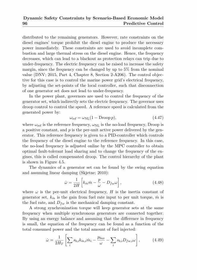
96Dynamic Safety Constraints by Scenario-Based Economic Model
Predictive Control
distributed to the remaining generators. However, rate constraints on thediesel engines’ torque prohibit the diesel engine to produce the necessarypower immediately. These constraints are used to avoid incomplete com-bustion and large thermal stress on the diesel engine. Hence, the frequencydecreases, which can lead to a blackout as protection relays can trip due tounder-frequency. The electric frequency can be raised to increase the safetymargin, since the frequency can be changed by up to 5% from the nominalvalue (DNV; 2015, Part 4, Chapter 8, Section 2-A206). The control objec-tive for this case is to control the marine power grid’s electrical frequency,by adjusting the set-points of the local controller, such that disconnectionof one generator set does not lead to under-frequency.
In the power plant, governors are used to control the frequency of thegenerator set, which indirectly sets the electric frequency. The governor usesdroop control to control the speed. A reference speed is calculated from thegenerated power by:
ωref = ωNL(1−Droop p), (4.47)where ωref is the reference frequency, ωNL is the no-load frequency, Droop isa positive constant, and p is the per-unit active power delivered by the gen-erator. This reference frequency is given to a PID-controller which controlsthe frequency of the diesel engine to the reference frequency. In this case,the no-load frequency is adjusted online by the MPC controller to obtainoptimal fault-tolerant load sharing and to change the frequency of the en-gines, this is called compensated droop. The control hierarchy of the plantis shown in Figure 4.5.
The dynamics of a generator set can be found by the swing equationand assuming linear damping (Skjetne; 2010):
ω = 12H
[kmm−
p
ω−Dfwω
], (4.48)
where ω is the per-unit electrical frequency, H is the inertia constant ofgenerator set, km is the gain from fuel rate input to per unit torque, m isthe fuel rate, and Dfw is the mechanical damping constant.
A strong synchronization torque will keep generator sets at the samefrequency when multiple synchronous generators are connected together.By using an energy balance and assuming that the difference in frequencyis small, the equation of the frequency can be found as a function of thetotal consumed power and the total amount of fuel injected:
ω = 12HT
[∑i
sb,ikm,imi −pbus
ω−∑
i
sb,iDfw,iω
], (4.49)
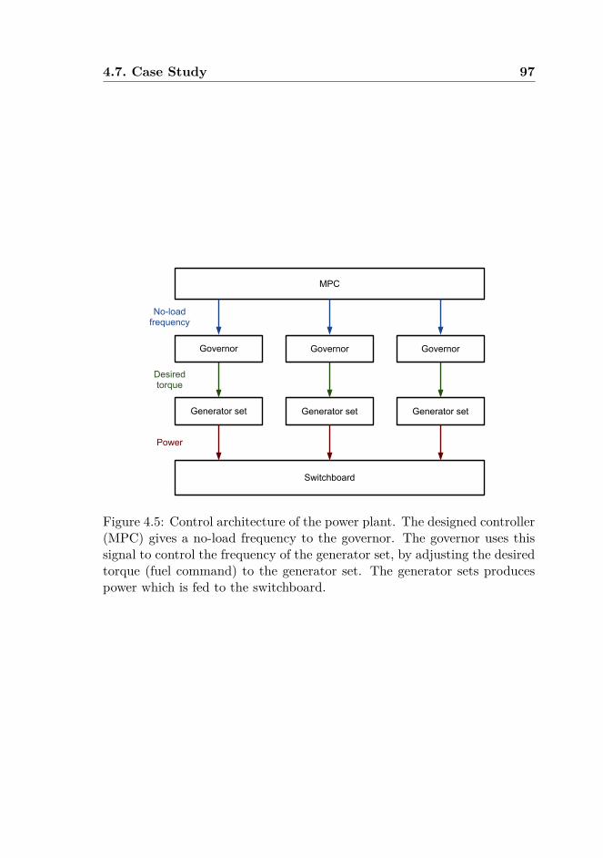
4.7. Case Study 97
MPC
No-load frequency
Desired torque
Switchboard
Power
Generator set
Governor
Generator set
Governor
Generator set
Governor
Figure 4.5: Control architecture of the power plant. The designed controller(MPC) gives a no-load frequency to the governor. The governor uses thissignal to control the frequency of the generator set, by adjusting the desiredtorque (fuel command) to the generator set. The generator sets producespower which is fed to the switchboard.
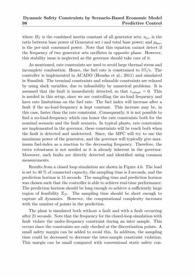
98Dynamic Safety Constraints by Scenario-Based Economic Model
Predictive Control
where HT is the combined inertia constant of all generator sets; sb,i, is theratio between base power of Generator set i and total base power; and pbus,is the per-unit consumed power. Note that this equation cannot detect ifthe frequency of two generator sets oscillates in opposite phase. However,this stability issue is neglected as the governor should take care of it.
As mentioned, rate constraints are used to avoid large thermal stress andincomplete combustion. Hence, the fuel rate is constrained to 5%/s. Thecontroller is implemented in ACADO (Houska et al.; 2011) and simulatedin Simulink. The terminal constraints and relaxable constraints are relaxedby using slack variables, due to infeasibility by numerical problems. It isassumed that the fault is immediately detected, so that τrobust = 0. Thisis needed in this setup, since we are controlling the no-load frequency andhave rate limitations on the fuel rate. The fuel index will increase after afault if the no-load-frequency is kept constant. This increase may be, inthis case, faster than the rate constraint. Consequently, it is not possible tofind a no-load-frequency which can honor the rate constraints both for thenominal scenario and the fault scenario. In typical plants, rate constraintsare implemented in the governor, these constraints will be reach both whenthe fault is detected and undetected. Since, the MPC will try to use themaximum power of the generator, and the governor will typically give max-imum fuel-index as a reaction to the decreasing frequency. Therefore, theextra robustness is not needed as it is already inherent in the governor.Moreover, such faults are directly detected and identified using commonmeasurements.
Results from a closed loop simulation are shown in Figure 4.6. The loadis set to 40 % of connected capacity, the sampling time is 3 seconds, and theprediction horizon is 15 seconds. The sampling time and prediction horizonwas chosen such that the controller is able to achieve real-time performance.The prediction horizon should be long enough to achieve a sufficiently largeregion of feasibility XN . The sampling time should be short enough tocapture all dynamics. However, the computational complexity increaseswith the number of points in the prediction.
The plant is simulated both without a fault and with a fault occurringafter 21 seconds. Note that the frequency for the closed-loop simulation withfault violate the under-frequency constraint during an inter sample. Thisoccurs since the constraints are only checked at the discretization points. Asmall safety margin can be added to avoid this. In addition, the samplingtime could be decreased to decrease the inter-sample constraint violation.This margin can be small compared with conventional static safety con-
4.7. Case Study 99
0 10 20 30 40 50
Time [s]
0.94
0.96
0.98
1.00
1.02
Fre
qu
ency
[p.u
.]
Figure 4.6: Closed-loop simulation of the case plant. The solid blue lineshows the closed-loop trajectory during nominal (fault free) operation. Thedashed green line shows the closed-loop trajectory when simulating that afault occurs after 21 seconds. The dotted red line shows the under-frequencylimit. Note that the frequency of the faulty system violates the under-frequency constraint during an inter sample, this occurs since the constraintsare only checked at the discretization points in the trajectory (dots in thetrajectory).
straints, since it should only take care of numerical and model errors, andnot the fault dynamics. The frequency is often controlled close to the ratedvalue when controlling the frequency of marine diesel-electric power plant.The electric load is normally reduced after the fault is detected to avoidunder-frequency. However, in this case this is unnecessary and undesired,as the fault must be detected and the operation may be interrupted. Thefrequency drop can be reduced by adding more diesel engines to the grid;however, this decreases the efficiency of the power plant. The frequencyafter the fault settles down close to the nominal frequency, since the recov-erable controller is tuned to control the frequency to the nominal frequency.This is generally considered as the safest frequency after a fault.
Since we have relaxed the constraints in this simulation, N∗relaxed isequal to N, which means that N∗relaxed is not a good measure for the fault-preparedness. However, the size of the slack variables will give a good indi-cation of preparedness for fault in the plant. One method for preparednessindication could be to set a threshold on the size of the slack variables, suchthat the plant is considered as prepared for faults when all slack variablesare less than this threshold. This threshold can be found by system knowl-edge and should correspond to the size of the safety margin mentioned inthe previous paragraph.
The optimization problem consists of 195 optimization variables and157 constraints. The computational time is between 0.5 and 2.5 seconds per

100Dynamic Safety Constraints by Scenario-Based Economic Model
Predictive Control
update period, when using ACADOs C++ interface and a 3.4 GHz Intel R©
CoreTM i7 processor. Note that ACADO’s C++ interface is not designed forconstraints that combine constraints at different time instances, such as theinitial constraint of a fault trajectory
(e.g., x(n)(t1) = Ejx(fj)(t0|tf = t1)
).
This is by-passed by adding auxiliary optimization variables. Therefore,the implemented optimization problem can be substantially condensed. Itis also the authors’ experience that using ACADO’s c-code export functionwill give a significant performance improvement (typically 10 to 100 timesfaster).
4.8 ConclusionThis chapter proposes a method to introduce safety constraints based onfault scenarios. The controller uses the fault scenarios internally in themodel predictive controller to make sure that it controls the states to a stateset where the plant is recoverable if faults occur. The advantages of the con-troller is less conservative safety constraint, and exact safety constraints arenot needed. The disadvantage is a larger and more computational expen-sive optimization problem, in addition to the need to identify and modelthe fault scenarios.
The performance of the controller was tested by closed-loop simulationof a linear plant and a marine power plant with relaxed constraints. Thesimulations show that the controller fulfills the control objectives as long asa safety margin is used, even when the constraints are relaxed.
Chapter 5
Battery Peak-ShavingControl in Electric MarinePower Plant using NonlinearModel Predictive Control
This chapter is based on Bø and Johansen (n.d.a).
5.1 Introduction
On some marine vessels the power consumption fluctuates heavily in certainoperational and environmental conditions. This combined with the weakpower grid gives problems such as fluctuating frequencies, excessive wearand tear of power producers, and synchronization problem when connectingadditional generator sets. Currently this problem is solved by connectingadditional generators, which gives a stiffer grid, but reduces the efficiencyof the plant, and increases the need for maintenance. Recently, it has beensuggested to add batteries to the power plant. The batteries can be usedfor peak-shaving, while the generator sets produce slowly varying power tomeet the demand.
The batteries used for this task must be able to charge and dischargelarge currents. However, the storage capacity can be small, since the meancurrent is zero. One problem with such large charge and discharge currentis the produced heat. This heat production must be controlled, else the bat-teries will be disconnected due to overheating. For some vessel the batteries
101
102Battery Peak-Shaving Control in Electric Marine Power Plant
using Nonlinear Model Predictive Control
can be used for emergency power, this require a larger battery bank, whichis less exposed to heat challenges.
The power fluctuation on a vessel may come from heave-compensators,auxiliary systems, hotel loads, and thrusters. Typically, the load periodsvary from 0.1 seconds to hundreds of seconds. The diesel engines wouldlike to have as constant load as possible, since this reduces the thermalstress due to temperature transients. Diesel engines have difficulties withcompensating for loads with dynamics faster than about 10 seconds, dueto the turbo-lag. On the other hand, the inertia of the generator set cancompensate for some load fluctuation. Typically, the inertia can handledynamics faster than 2 seconds. However, this increases the mechanicalstress on the generator set. On a marine vessel the total produced powercan be measured at the generators. This is often done every 0.1 second.
Therefore, the peak-shaving algorithm should handle fluctuations withperiods from 0.1 seconds to 100 seconds, and most important, take care ofloads fluctuations with periods between 2 seconds and 10 seconds.
A dynamic approach should be chosen, so that most of the load fluc-tuations are removed. However, only the most important load fluctuationsshould be removed when the battery starts to get too warm. The tempera-ture dynamics of the batteries is slow, and it may take several hours to coolthem down. We therefore suggest a hierarchy of controllers, with a high-level controller, which selects the periods of the load fluctuations to cancelout. And, a low-level controller, which takes care of the peak-shaving byremoving the periods given by the high-level controller.
Alternative methods to reduce power fluctuations on marine vessels hasalready been proposed. It is proposed to use the thrust allocation andfeedforward in the governor to reduce the power fluctuations (Mathiesenet al.; 2012; Veksler et al.; 2012b). Another approach is to use the thrustersdirectly for peak-shaving by generating a thruster load which counteractsother load variations (Radan et al.; 2008). Typically, thruster biasing is usedon DP vessels to reduce load variations. Then, thrusters are counteractingeach other to waste power, such that other load variations are canceledout (Shi et al.; 2011). The mass of the vessel can also be used to reduce thepower fluctuations if a drift force is present (Johansen et al.; 2014). Noneof these employ batteries for energy storage.
Batteries are starting to be used in marine vessels. MS Viking Queenwill soon be retrofitted with batteries (Eidsvik; 2015), while MS Ampereis in operation and is only driven by batteries (Martini; 2015). It is alsosuggested to use batteries on naval vessels, which can take care of pulse
5.1. Introduction 103
loads from weapon systems (Huhman and Wetz; 2015; Kuznetsov; 2015).Batteries can also be used for emergency power, as demonstrated in Kimet al. (2015).
The problem of adapting time constants for the peak-shaving algorithmhas similarities with the power split problem for hybrid electric vehicles,where the desired torque is generated by a combustion engine and an elec-tric motor with a battery. Many different strategies are suggested, for theoriginal Toyota Prius a rule based controller was used (Hermance and Sasaki;1998). Stochastic model predictive control has been suggested (Moura et al.;2011), as well as using dynamic programming for design of a rule based con-troller (Lin et al.; 2003). A controller which optimize fuel consumption andemissions is presented in Johnson et al. (2000). Battery energy storagesystems (BESS) are also proposed for wind turbine plants. BESS can beused to smooth the power fluctuations due to the variations of the windspeed (Hovgaard et al.; 2013; Sebastián and Quesada; 2006; Zeng et al.;2006). Kottick et al. (1993) demonstrated how BESS can be used in anisolated power grid to reduce frequency variations.
Model predictive control (MPC) is used in this chapter as a high-levelcontroller. A model of the plant is used in the MPC to predict the futurestate of the system. A cost function is used to evaluate the future per-formance of the system. The MPC optimizes the cost for the predictionhorizon. At every step the free variables are optimized with respect to thecost function and constraints, and only the variables for the first step isapplied on the system. There already exists multiple suggestion for use ofMPC in marine power plants, such as Bø and Johansen (2013); Park et al.(2015); Stone et al. (2015); Veksler et al. (2012b).
We will use probabilistic constraints in this chapter, since future loadprediction is uncertain. These are constraints on the form Prob(X < xmin) < η,where Prob(·) is the probability, 0 < η 1 is the probability threshold andX is a stochastic variable. For a linear system with Gaussian disturbance itis shown that the constraints can be converted to an explicit second ordercone constraint (Hovgaard et al.; 2011; Oldewurtel et al.; 2010). It is alsosuggested to use scenarios and conditional value at risk as an approximationof the probabilistic constraint (Hanssen et al.; 2015). An approximationusing scenario and mixed integer quadratic programming is presented inMatusko and Borrelli (2012).
The main contribution of this chapter is a controller which can adap-tively optimize parameters based on estimates of the power spectrum den-sity. It is applied to optimal tuning of peak-shaving. This is done with

104Battery Peak-Shaving Control in Electric Marine Power Plant
using Nonlinear Model Predictive Control
batteries to smooth out the power demand of a marine vessel. The batteryis controlled by a band-pass filter, so that only power variations in a givenfrequency band are counteracted.
5.2 Control Plant
The control architecture is shown in Figure 5.1. A load consumes the loadPLoad, where PLoad is stochastic with the power spectrum ppp(ω). A batteryis used to smooth the fluctuations in the generated power. The goal is tokeep the temperature and state of charge of the battery within the opera-tional limits, while reducing the power fluctuations on the generator set asmuch as possible.
The charging and discharging power of the battery are given by a band-pass filter. The input to the band-pass filter is Pload, while the output is thedesired charging power, Pref. The MPC adjusts the time constants of theband-pass filter to avoid too high battery temperatures. This cancels outpower fluctuations with frequencies between the cut-off frequencies of theband-pass filter. This will give a zero-mean charging power of the battery.However, the battery will still be discharged even with zero-mean chargingpower, due to losses in the battery. Consequently, the MPC gives a meancharging power, PMCP, to control the mean state of charge (SoC).
It should be noted that measurements of the generated power may notbe synchronized and may have measurement errors. We assume that thetotal consumed and generated power is measured without any measurementerrors, in this study.
A first order high-pass filter and low-pass filter are put in series to im-plement a band-pass filter. However, any linear band-pass filter could havebeen chosen. The transfer function for this filter is:
Hf (s) = Pref(s)Pload(s) = τ s
(1 +¯τs)(1 + τ s)ncells
(5.1)
where τ and¯τ are the highest and lowest time constant of the band pass
filter, and ncells is the number of cells in the battery.A simple model is used for the battery, as shown in Figure 5.2. The
internal resistance, Ri, and open circuit voltage, Vo, are assumed to beconstant. The temperature of the battery is modeled by Newtons law ofcooling:
dTdt = hA
c(Tair − T ) + 1
cQel (5.2)
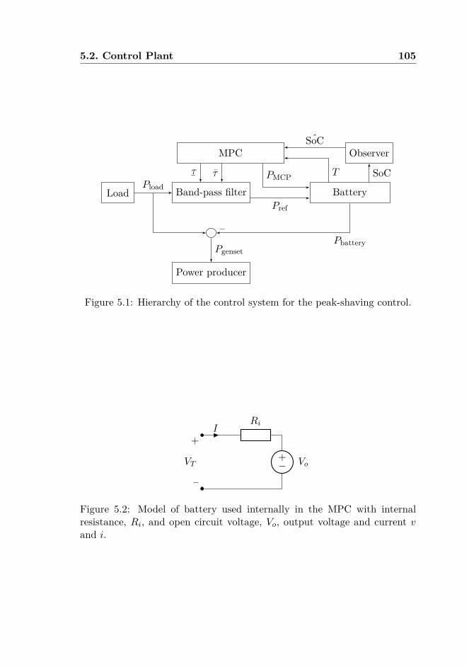
5.2. Control Plant 105
Band-pass filterLoad Battery
Power producer
Pload
Pref
MPC Observer
¯τ τ SoCTPMCP
Pbattery
–
Pgenset
ˆSoC
Figure 5.1: Hierarchy of the control system for the peak-shaving control.
+− Vo
RiI
−
+
VT
Figure 5.2: Model of battery used internally in the MPC with internalresistance, Ri, and open circuit voltage, Vo, output voltage and current vand i.

106Battery Peak-Shaving Control in Electric Marine Power Plant
using Nonlinear Model Predictive Control
where T is the battery temperature, h heat transfer coefficient, A is thesurface area of the battery, c is the heat capacity of the battery, Tair is thetemperature of the cooling air, and Qel is the heat generated in the battery.The heat is assumed to be equal to the electrical loss
Qel = RiI2 (5.3)
where I is the current through the battery.Due to safety requirements the battery has a temperature limit for op-
eration:T ≤ Tmax (5.4)
The battery must be disconnected when this level is reached.The charging power is controlled by a bi-directional AC/DC converter,
and it is controlled to the sum of the reference from the band-pass filter andthe MPC:
Pbattery = Pref + PMP C (5.5)
Setting Pbattery = I(Vo +RiI), and solving for the current, we get:
I =−Vo +
√V 2
o + 4RiPbattery
2Ri
= PbatteryVo
−P 2
batteryRi
V 3o
+O(P 3battery) (5.6)
The SoC of the battery is modeled as an integrator of the current (Mouraet al.; 2011):
dSoCdt = I
Qnominal(5.7)
where Qnominal is the rated charge of the battery. Hence, the SoC of thebattery is 0 when depleted and 1 when fully charged. It is assumed thatSoC is measured or estimated, as SoC estimates from Coulomb countingwill drift-off. There exists multiple methods for such estimation, e.g. Kim(2008); Piller et al. (2001); Plett (2004). The SoC is also constrained:
SoCmin ≤ SoC ≤ SoCmax (5.8)
The minimum and maximum state of charge, can be set by an operator ora plant optimizer. SoCmin and SoCmax can be used to avoid accelerated
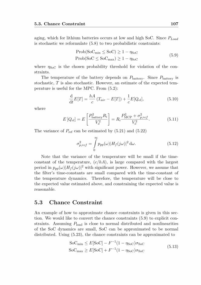
5.3. Chance Constraint 107
aging, which for lithium batteries occurs at low and high SoC. Since PLoad
is stochastic we reformulate (5.8) to two probabilistic constraints:
Prob(SoCmin ≤ SoC) ≥ 1− ηSoC
Prob(SoC ≤ SoCmax) ≥ 1− ηSoC(5.9)
where ηSoC is the chosen probability threshold for violation of the con-straints.
The temperature of the battery depends on Pbattery. Since Pbattery isstochastic, T is also stochastic. However, an estimate of the expected tem-perature is useful for the MPC. From (5.2):
ddtE[T ] = hA
c(Tair − E[T ]) + 1
cE[Qel], (5.10)
where
E [Qel] = E
[P 2
batteryRi
V 2o
]= Ri
P 2MCP + σ2
p,ref
V 2o
. (5.11)
The variance of Pref can be estimated by (5.21) and (5.22)
σ2p,ref =
∞∫0
ppp(ω)|Hf (jω)|2 dω. (5.12)
Note that the variance of the temperature will be small if the time-constant of the temperature, (c/hA), is large compared with the largestperiod in ppp(ω)|Hf (jω)|2 with significant power. However, we assume thatthe filter’s time-constants are small compared with the time-constant ofthe temperature dynamics. Therefore, the temperature will be close tothe expected value estimated above, and constraining the expected value isreasonable.
5.3 Chance ConstraintAn example of how to approximate chance constraints is given in this sec-tion. We would like to convert the chance constraints (5.9) to explicit con-straints. Assuming Pload is close to normal distributed and nonlinearitiesof the SoC dynamics are small, SoC can be approximated to be normaldistributed. Using (5.23), the chance constraints can be approximated to
SoCmin ≤ E[SoC]− F−1(1− ηSoC)σSoC
SoCmax ≥ E[SoC] + F−1(1− ηSoC)σSoC(5.13)

108Battery Peak-Shaving Control in Electric Marine Power Plant
using Nonlinear Model Predictive Control
where F−1(·) is the inverse cumulative distribution function of the standardnormal distribution.
An estimate of E[SoC] and σ2SoC is needed. We get:
ddtE [SoC] = E
[Pbattery
VoQnominal−
P 2batteryRi
V 3o Qnominal
]
= PMCPVoQnominal
−(P 2
MCP + σ2p,ref)Ri
V 3o Qnominal
(5.14)
by using (5.5), (5.6), and (5.7), neglecting third and higher order terms, andutilizing E[Pref] = 0.
The variance of SoC can be estimated by linearizing (5.6). This gives alinear system from Pload to SoC.
σ2SoC ≈
∞∫0
ppp(ω) |Hf (jω)|2
Q2nominalV
2o
dω (5.15)
The state of charge can be seen as a slowly varying mean, E[SoC], witha superimposed noise.
SoC = E[SoC] + v, (5.16)
where v is the measurement noise. E[SoC] is then the initial conditionof (5.14). To estimate E[SoC] a discrete Kalman filter is applied, whereSoC is the measured state. The process is modeled as:
d ˆSoCdt = PMCP
VoQnominal−
(P 2MCP + σ2
p,ref)Ri
V 3o Qnominal
+ w (5.17)
y = ˆSoC + v (5.18)
where ˆSoC is the estimated E[SoC], w is the process noise, and v is themeasurement noise. The variance of v is assumed to be white noise withvariance σ2
SoC. The variance of w is a tunning parameter for the filter, whichincludes model errors. More details about Kalman filters can be found ine.g., Brown and Hwang (1997, Chapter 5).
Both E[SoC] and σSoC can be controlled to fulfill (5.13). It was ob-served during the simulation study that when both E[SoC] and σSoC arecontrolled the optimal solution is sometime to reduce σSoC by decreasingthe distance between
¯τ and τ . However, the desired performance is that
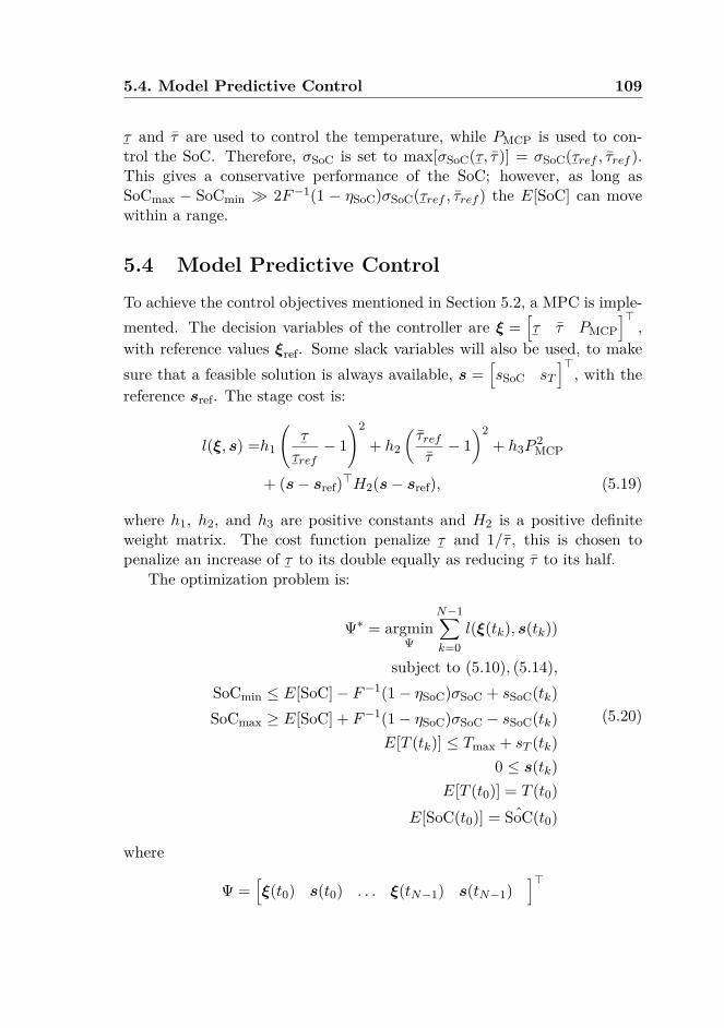
5.4. Model Predictive Control 109
¯τ and τ are used to control the temperature, while PMCP is used to con-trol the SoC. Therefore, σSoC is set to max[σSoC(
¯τ, τ)] = σSoC(
¯τref , τref ).
This gives a conservative performance of the SoC; however, as long asSoCmax − SoCmin 2F−1(1 − ηSoC)σSoC(
¯τref , τref ) the E[SoC] can move
within a range.
5.4 Model Predictive Control
To achieve the control objectives mentioned in Section 5.2, a MPC is imple-mented. The decision variables of the controller are ξ =
[¯τ τ PMCP
]>,
with reference values ξref. Some slack variables will also be used, to makesure that a feasible solution is always available, s =
[sSoC sT
]>, with the
reference sref. The stage cost is:
l(ξ, s) =h1
(¯τ
¯τref− 1
)2
+ h2
(τref
τ− 1
)2+ h3P
2MCP
+ (s− sref)>H2(s− sref), (5.19)
where h1, h2, and h3 are positive constants and H2 is a positive definiteweight matrix. The cost function penalize
¯τ and 1/τ , this is chosen to
penalize an increase of¯τ to its double equally as reducing τ to its half.
The optimization problem is:
Ψ∗ = argminΨ
N−1∑k=0
l(ξ(tk), s(tk))
subject to (5.10), (5.14),SoCmin ≤ E[SoC]− F−1(1− ηSoC)σSoC + sSoC(tk)SoCmax ≥ E[SoC] + F−1(1− ηSoC)σSoC − sSoC(tk)
E[T (tk)] ≤ Tmax + sT (tk)0 ≤ s(tk)
E[T (t0)] = T (t0)E[SoC(t0)] = ˆSoC(t0)
(5.20)
where
Ψ =[ξ(t0) s(t0) . . . ξ(tN−1) s(tN−1)
]>
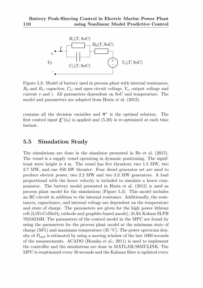
110Battery Peak-Shaving Control in Electric Marine Power Plant
using Nonlinear Model Predictive Control
+− Vo(T, SoC)
R0(T, SoC)R1(T, SoC)
C1(T, SoC)
I
−
+
VT
Figure 5.3: Model of battery used in process plant with internal resistances,R0 and R1; capacitor, C1; and open circuit voltage, Vo, output voltage andcurrent v and i. All parameters dependent on SoC and temperature. Themodel and parameters are adapted from Huria et al. (2012).
contains all the decision variables and Ψ∗ is the optimal solution. Thefirst control input ξ∗(t0) is applied and (5.20) is re-optimized at each timeinstant.
5.5 Simulation Study
The simulations are done in the simulator presented in Bø et al. (2015).The vessel is a supply vessel operating in dynamic positioning. The signif-icant wave height is 4 m. The vessel has five thrusters, two 1.5 MW, two2.7 MW, and one 850 kW thruster. Four diesel generator set are used toproduce electric power, two 2.2 MW and two 3.3 MW generators. A loadproportional with the heave velocity is included to simulate a heave com-pensator. The battery model presented in Huria et al. (2012) is used asprocess plant model for the simulations (Figure 5.3). This model includesan RC-circuit in addition to the internal resistance. Additionally, the resis-tances, capacitance, and internal voltage are dependent on the temperatureand state of charge. The parameters are given for the high power lithiumcell (LiNi-CoMnO2 cathode and graphite-based anode), 31Ah Kokam SLPB78216216H. The parameters of the control model in the MPC are found byusing the parameters for the process plant model at the minimum state ofcharge (50%) and maximum temperature (35 C). The power spectrum den-sity of Pload is estimated by using a moving window of the last 1000 secondsof the measurements. ACADO (Houska et al.; 2011) is used to implementthe controller and the simulations are done in MATLAB/SIMULINK. TheMPC is reoptimized every 50 seconds and the Kalman filter is updated every
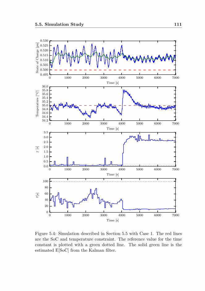
5.5. Simulation Study 111
0 1000 2000 3000 4000 5000 6000 7000
Time [s]
0.495
0.500
0.505
0.510
0.515
0.520
0.525
0.530S
tate
of
Ch
arg
e[p
u]
0 1000 2000 3000 4000 5000 6000 7000
Time [s]
34.234.434.634.835.035.235.435.635.836.0
Tem
per
atu
re[
C]
0 1000 2000 3000 4000 5000 6000 7000
Time [s]
0.0
0.5
1.0
1.5
2.0
2.5
3.0
3.5
¯τ[s
]
0 1000 2000 3000 4000 5000 6000 7000
Time [s]
0
20
40
60
80
100
τ[s
]
Figure 5.4: Simulation described in Section 5.5 with Case 1. The red linesare the SoC and temperature constraint. The reference value for the timeconstant is plotted with a green dotted line. The solid green line is theestimated E[SoC] from the Kalman filter.
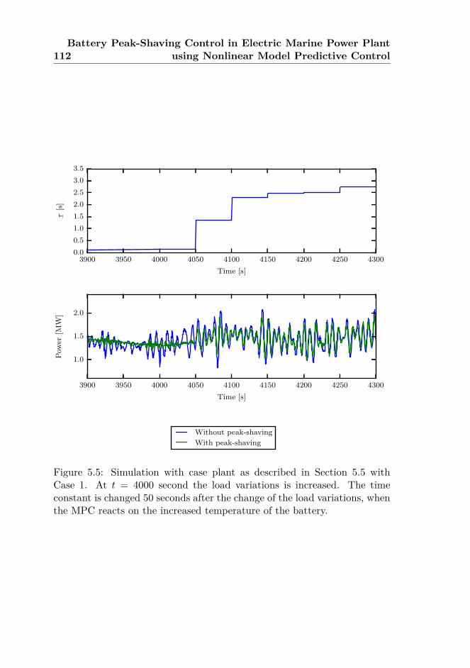
112Battery Peak-Shaving Control in Electric Marine Power Plant
using Nonlinear Model Predictive Control
3900 3950 4000 4050 4100 4150 4200 4250 4300
Time [s]
0.0
0.5
1.0
1.5
2.0
2.5
3.0
3.5
¯τ[s
]
3900 3950 4000 4050 4100 4150 4200 4250 4300
Time [s]
1.0
1.5
2.0
Pow
er[M
W]
Without peak-shaving
With peak-shaving
Figure 5.5: Simulation with case plant as described in Section 5.5 withCase 1. At t = 4000 second the load variations is increased. The timeconstant is changed 50 seconds after the change of the load variations, whenthe MPC reacts on the increased temperature of the battery.
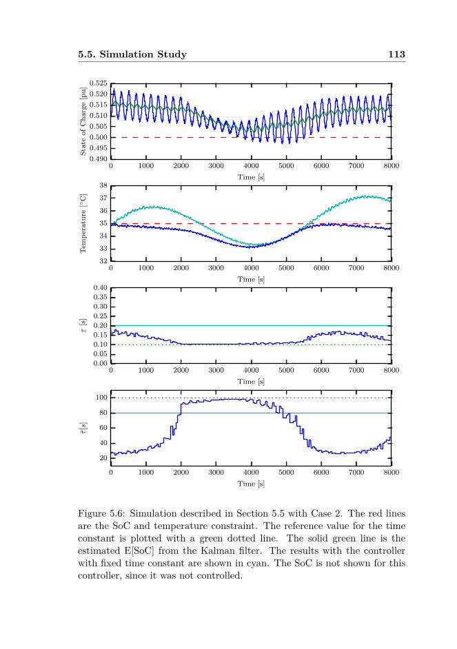
5.5. Simulation Study 113
0 1000 2000 3000 4000 5000 6000 7000 8000
Time [s]
0.490
0.495
0.500
0.505
0.510
0.515
0.520
0.525S
tate
of
Ch
arg
e[p
u]
0 1000 2000 3000 4000 5000 6000 7000 8000
Time [s]
32
33
34
35
36
37
38
Tem
per
atu
re[
C]
0 1000 2000 3000 4000 5000 6000 7000 8000
Time [s]
0.00
0.05
0.10
0.15
0.20
0.25
0.30
0.35
0.40
¯τ[s
]
0 1000 2000 3000 4000 5000 6000 7000 8000
Time [s]
20
40
60
80
100
τ[s
]
Figure 5.6: Simulation described in Section 5.5 with Case 2. The red linesare the SoC and temperature constraint. The reference value for the timeconstant is plotted with a green dotted line. The solid green line is theestimated E[SoC] from the Kalman filter. The results with the controllerwith fixed time constant are shown in cyan. The SoC is not shown for thiscontroller, since it was not controlled.
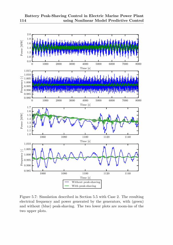
114Battery Peak-Shaving Control in Electric Marine Power Plant
using Nonlinear Model Predictive Control
0 1000 2000 3000 4000 5000 6000 7000 8000
Time [s]
0.8
1.0
1.2
1.4
1.6
1.8
2.0
Pow
er[M
W]
0 1000 2000 3000 4000 5000 6000 7000 8000
Time [s]
0.980
0.985
0.990
0.995
1.000
1.005
1.010
1.015
Fre
qu
ency
[-]
1060 1080 1100 1120 1140
Time [s]
1.0
1.1
1.2
1.3
1.4
1.5
1.6
1.7
Pow
er[M
W]
1060 1080 1100 1120 1140
Time [s]
0.985
0.990
0.995
1.000
1.005
1.010
Fre
qu
ency
[-]
Without peak-shaving
With peak-shaving
Figure 5.7: Simulation described in Section 5.5 with Case 2. The resultingelectrical frequency and power generated by the generators, with (green)and without (blue) peak-shaving. The two lower plots are zoom-ins of thetwo upper plots.
5.5. Simulation Study 115
10 second, with σ2w = 4×10⁻⁸. The remaining parameters in the simulation
are given in Table 5.1.Two cases are simulated. In Case 1, the standard deviation of the heave
compensator is 50 kW the first 4000 seconds, thereafter it is increased to200 kW. A data series of 3000 seconds is generated and repeated three times.This is done to exemplify the steady-state performance of the controller.Results are shown in Fig 5.4 and 5.5. In Case 2 the standard deviationof heave compensator is 50 kW. However, a complete time series is usedto illustrate the adaptiveness when the variance is slowly changing. Thepresent controller is compared with a peak-shaving controller where
¯τ = 0.2
seconds and τ = 80 seconds. Results are shown in Figure 5.6.Results from the simulation with Case 1 are shown in Figure 5.4. It is
clear that the time average of the SoC is controlled to a level above SoCmin.The variance of the temperature is also small; therefore, it is reasonable toconstrain the expected temperature and not necessary to use probabilisticconstraints. After 4000 seconds the temperature increases rapidly due tothe increase variations in the power demand. However, the controller takesaction at the first update of the MPC after battery temperature starts toincrease. Therefore, a safety margin on the temperature limit is needed toavoid disconnection of the battery, due to over-temperature. Details on thetransition after 4000 seconds are shown in Figure 5.5. Most of the loadfluctuations are canceled out until 4050 seconds. At this instant the timeconstants are changed to reduce the increased temperature. The band-passfilter is narrowed to time constants of 3 and 7 seconds, which is typicallythe most difficult time scales for the diesel engines.
Results from the simulation of Case 2 are shown in Figure 5.6 and 5.7.During this simulation the variance of Pload is slowly changing. The timeconstants of the bandpass filter are changed dynamical, such that it is widewhen the battery temperature is low, and narrow when its high. It maintainsthe temperature below the temperature limits when the variance increases.In contrast, the fixed time constant approach gives too high temperatures,and the filter does not utilize the full potential of the peak-shaving capabilitywhen the temperature is low. This approach requires either tuning of thefilter often or a very conservative tuning. Between 3500 and 4500 seconds,when the fluctuations increases again, the SoC constraint (5.8) is violated11.5% of the time. This is mainly due to the lag of the estimation of thepower spectrum density.
Simulation results with and without peak-shaving are shown in Fig-ure 5.7, which shows the power demand on the generator sets and electrical
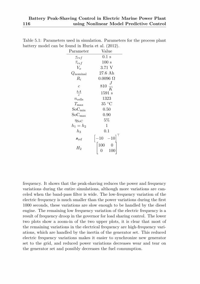
116Battery Peak-Shaving Control in Electric Marine Power Plant
using Nonlinear Model Predictive Control
Table 5.1: Parameters used in simulation. Parameters for the process plantbattery model can be found in Huria et al. (2012).
Parameter Value
¯τref 0.1 sτref 100 sVo 3.71 V
Qnominal 27.6 AhRi 0.0096 Ω
c 810 J
KhAc 1591 s
ncells 1323Tmax 35 C
SoCmin 0.50SoCmax 0.90ηSoC 5%
h1 = h2 1h3 0.1sref
[−10 −10
]>H2
[100 00 100
]
frequency. It shows that the peak-shaving reduces the power and frequencyvariations during the entire simulations, although more variations are can-celed when the band-pass filter is wide. The low-frequency variation of theelectric frequency is much smaller than the power variations during the first1000 seconds, these variations are slow enough to be handled by the dieselengine. The remaining low frequency variation of the electric frequency is aresult of frequency droop in the governor for load sharing control. The lowertwo plots show a zoom-in of the two upper plots, it is clear that most ofthe remaining variations in the electrical frequency are high-frequency vari-ations, which are handled by the inertia of the generator set. This reducedelectric frequency variations makes it easier to synchronize new generatorset to the grid, and reduced power variations decreases wear and tear onthe generator set and possibly decreases the fuel consumption.
5.6. Conclusion 117
5.6 ConclusionIt is demonstrated in this chapter how the power spectrum density can beused to estimate expected values and variance of state of charge and ex-pected temperatures of a battery. This is used in the optimization problemof the MPC. A peak-shaving example was used to demonstrate the con-trol scheme. The MPC sets time constants of a band-pass filter, whichcontrols the peak-shaving done by the battery. The controllers objectiveis to maintain a battery temperature below a maximum temperature anda state of charge within a desired range. It is shown that the controllerachieves its control objective, by controlling the temperature and state ofcharge close to the constraint. However, the constraints are violated after asudden change of the disturbance. The peak-shaving algorithm cancels outthe variations that are most difficult to handle by the diesel engines, thisgives less variations on the electric frequency.
5.7 Appendix: Mathematical PreliminariesGiven a linear system with stochastic input w, transfer function H(s), andoutput x. The power spectrum density of w is pww(ω). For such a system,the power spectrum density of x is
pxx(ω) = pww(ω)|H(jω)|2. (5.21)
The variance and power of the signal are given as:
σ2x =
∞∫0
pxx(ω) dω. (5.22)
Given a normal distributed variable X, with the mean and variance xand σ2. The probability constraint:
Prob(X > xc) ≥ 1− η
is equivalent to
xc < x− F−1(1− η)σ (5.23)
where η is the probability threshold, and F−1(·) is the inverse probabilitydistribution of standard normal distribution.

118Battery Peak-Shaving Control in Electric Marine Power Plant
using Nonlinear Model Predictive Control
Chapter 6
Dynamic Positioning Systemas Dynamic Energy Storageon Diesel-Electric Ships
This chapter is a reformatted version of Johansen et al. (2014).
6.1 IntroductionDynamically positioned (DP) vessels with diesel-electric power and propul-sion systems are commonly used in offshore operations in order to keepthe ship position and heading at their references. While the DP systemis often the main consumer of electric power on the ship, other variablepower consumers are connected on the same power buses as the electricthrusters. The relatively weak electric grid on a vessel is therefore subjectto significant variations in voltage and frequency caused by the dynamicsof several more or less independent consumers. This causes challenges dueto increased wear and tear, maintenance costs, emissions, and fuel ineffi-ciency of diesel generators in combination with increased risk for blackoutdue to over- or under-frequency condition causing protection relays to tripgenerators. Common variable load consumers include drilling drives, heavecompensators, cranes, pumps and winches whose operation are often influ-enced by wave-induced ship motions and other external disturbances. Afurther benefit of dynamic energy storage is increased operational flexibilityas it allows these consumers to have higher priority than DP thrusters withrespect to load reduction and load shedding, without reduced safety or op-erational performance, for short periods of time. Dynamic energy storage
119
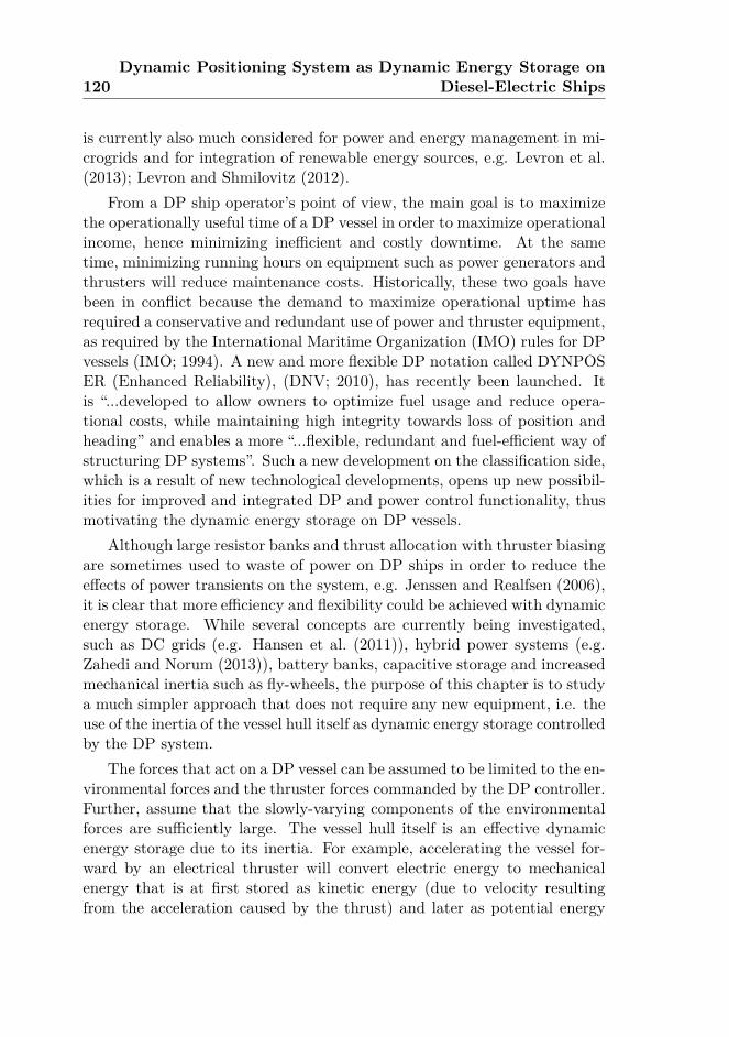
120Dynamic Positioning System as Dynamic Energy Storage on
Diesel-Electric Ships
is currently also much considered for power and energy management in mi-crogrids and for integration of renewable energy sources, e.g. Levron et al.(2013); Levron and Shmilovitz (2012).
From a DP ship operator’s point of view, the main goal is to maximizethe operationally useful time of a DP vessel in order to maximize operationalincome, hence minimizing inefficient and costly downtime. At the sametime, minimizing running hours on equipment such as power generators andthrusters will reduce maintenance costs. Historically, these two goals havebeen in conflict because the demand to maximize operational uptime hasrequired a conservative and redundant use of power and thruster equipment,as required by the International Maritime Organization (IMO) rules for DPvessels (IMO; 1994). A new and more flexible DP notation called DYNPOSER (Enhanced Reliability), (DNV; 2010), has recently been launched. Itis “...developed to allow owners to optimize fuel usage and reduce opera-tional costs, while maintaining high integrity towards loss of position andheading” and enables a more “...flexible, redundant and fuel-efficient way ofstructuring DP systems”. Such a new development on the classification side,which is a result of new technological developments, opens up new possibil-ities for improved and integrated DP and power control functionality, thusmotivating the dynamic energy storage on DP vessels.
Although large resistor banks and thrust allocation with thruster biasingare sometimes used to waste of power on DP ships in order to reduce theeffects of power transients on the system, e.g. Jenssen and Realfsen (2006),it is clear that more efficiency and flexibility could be achieved with dynamicenergy storage. While several concepts are currently being investigated,such as DC grids (e.g. Hansen et al. (2011)), hybrid power systems (e.g.Zahedi and Norum (2013)), battery banks, capacitive storage and increasedmechanical inertia such as fly-wheels, the purpose of this chapter is to studya much simpler approach that does not require any new equipment, i.e. theuse of the inertia of the vessel hull itself as dynamic energy storage controlledby the DP system.
The forces that act on a DP vessel can be assumed to be limited to the en-vironmental forces and the thruster forces commanded by the DP controller.Further, assume that the slowly-varying components of the environmentalforces are sufficiently large. The vessel hull itself is an effective dynamicenergy storage due to its inertia. For example, accelerating the vessel for-ward by an electrical thruster will convert electric energy to mechanicalenergy that is at first stored as kinetic energy (due to velocity resultingfrom the acceleration caused by the thrust) and later as potential energy
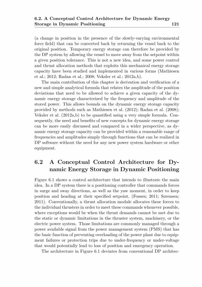
6.2. A Conceptual Control Architecture for Dynamic EnergyStorage in Dynamic Positioning 121
(a change in position in the presence of the slowly-varying environmentalforce field) that can be converted back by returning the vessel back to theoriginal position. Temporary energy storage can therefore be provided bythe DP system by allowing the vessel to move away from the setpoint withina given position tolerance. This is not a new idea, and some power controland thrust allocation methods that exploits this mechanical energy storagecapacity have been studied and implemented in various forms (Mathiesenet al.; 2012; Radan et al.; 2008; Veksler et al.; 2012a,b).
The main contribution of this chapter is derivation and verification of anew and simple analytical formula that relates the amplitude of the positiondeviations that need to be allowed to achieve a given capacity of the dy-namic energy storage characterized by the frequency and amplitude of thestored power. This allows bounds on the dynamic energy storage capacityprovided by methods such as Mathiesen et al. (2012); Radan et al. (2008);Veksler et al. (2012a,b) to be quantified using a very simple formula. Con-sequently, the need and benefits of new concepts for dynamic energy storagecan be more easily discussed and compared in a wider perspective, as dy-namic energy storage capacity can be provided within a reasonable range offrequencies and amplitudes simply through functions that can be realized inDP software without the need for any new power system hardware or otherequipment.
6.2 A Conceptual Control Architecture for Dy-namic Energy Storage in Dynamic Positioning
Figure 6.1 shows a control architecture that intends to illustrate the mainidea. In a DP system there is a positioning controller that commands forcesin surge and sway directions, as well as the yaw moment, in order to keepposition and heading at their specified setpoint, (Fossen; 2011; Sørensen;2011). Conventionally, a thrust allocation module allocates these forces tothe individual thrusters in order to meet these commands whenever possible,where exceptions would be when the thrust demands cannot be met due tothe static or dynamic limitations in the thruster system, machinery, or theelectric power system. Those limitations are commonly managed through apower available signal from the power management system (PMS) that hasthe basic function of preventing overloading of the power plant due to equip-ment failures or protection trips due to under-frequency or under-voltagethat would potentially lead to loss of position and emergency operation.
The architecture in Figure 6.1 deviates from conventional DP architec-
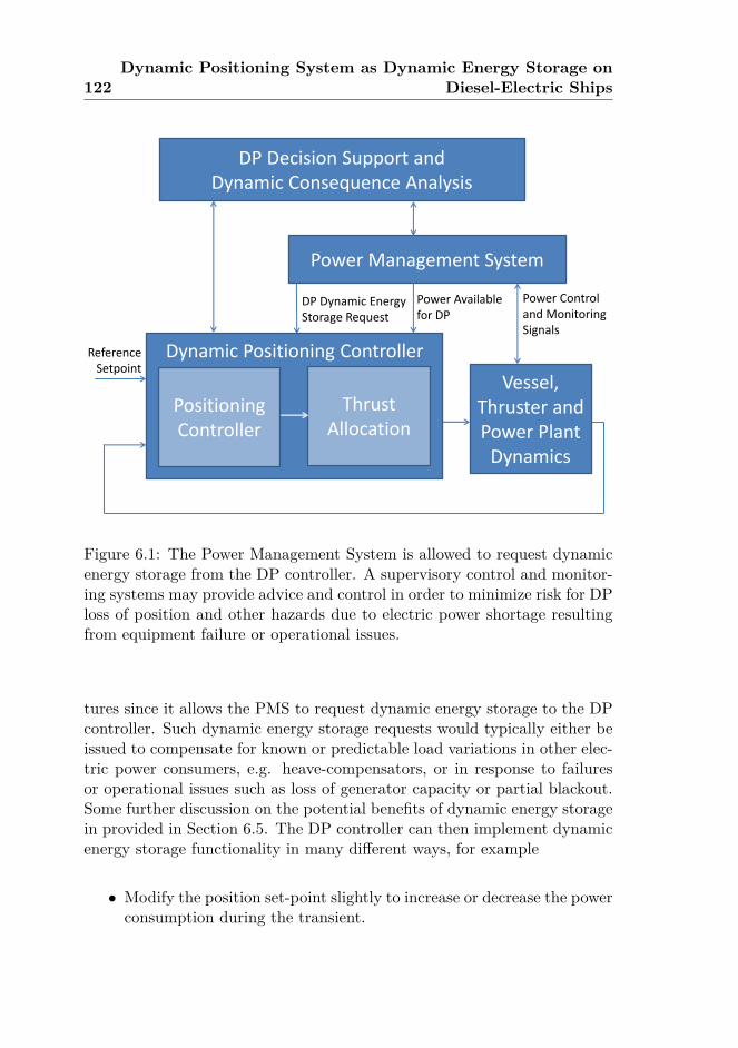
122Dynamic Positioning System as Dynamic Energy Storage on
Diesel-Electric Ships
Dynamic Positioning Controller
Thrust Allocation
Vessel, Thruster and Power Plant
Dynamics
Power Management System
Power Available for DP
DP Dynamic Energy Storage Request
Positioning Controller
Power Controland MonitoringSignals
DP Decision Support and Dynamic Consequence Analysis
ReferenceSetpoint
Figure 6.1: The Power Management System is allowed to request dynamicenergy storage from the DP controller. A supervisory control and monitor-ing systems may provide advice and control in order to minimize risk for DPloss of position and other hazards due to electric power shortage resultingfrom equipment failure or operational issues.
tures since it allows the PMS to request dynamic energy storage to the DPcontroller. Such dynamic energy storage requests would typically either beissued to compensate for known or predictable load variations in other elec-tric power consumers, e.g. heave-compensators, or in response to failuresor operational issues such as loss of generator capacity or partial blackout.Some further discussion on the potential benefits of dynamic energy storagein provided in Section 6.5. The DP controller can then implement dynamicenergy storage functionality in many different ways, for example
• Modify the position set-point slightly to increase or decrease the powerconsumption during the transient.
6.2. A Conceptual Control Architecture for Dynamic EnergyStorage in Dynamic Positioning 123
• Modify the thrust request to the thruster controllers, (Radan et al.;2008), without any analysis of consequences for positioning errors.
• Modify the thrust request to the thrust allocation with an amountthat corresponds to the requested dynamic energy storage rate. Thisis the approach that will be used in this chapter for demonstrationand analysis, for simplicity.
• Modify the power available and limits to the thrust allocation in orderto implement the dynamic energy storage request in a smooth andefficient way with minimum impact on the operation of the system,(Mathiesen et al.; 2012; Veksler et al.; 2012a,b).
Dynamic storage of energy as kinetic and potential energy in a DP ves-sel has some inherent limitations. First, the energy storage cannot changefaster than the thruster dynamics. While the electric thruster power can bechanged in much less time than one second using frequency converters, itshould be realized that persistent fast changes will cause mechanical stresson the system and increased tear and wear. Hence, in practice we expectthat energy storage dynamics faster than about 0.5 - 1 Hz cannot normallybe accommodated by the DP system. Note that higher frequencies thanthis would be effectively handled by the mechanical inertia of the diesel-generators, and the capacitances and inductances in the electric system,(Radan; 2008). On the other hand, the DP system typically has a controlbandwidth corresponding to a response time of 15-60 seconds for a typi-cal diesel-electric vessel. This bandwidth is chosen due to the dynamics ofthrusters as well as the desire to avoid to act against the first order wave in-duced motions, which is commonly achieved with wave filtering, (Sørensen;2011). Hence, energy dynamics slower than about 0.05 rad/sec, or about0.01 Hz, will be typically counteracted by the DP controller unless specialfunctionality is implemented to allow certain position deviations. Conse-quently, the DP dynamic energy storage will typically be mostly effectivefor power variations in the range of 0.01 Hz to 0.5 Hz. Although this is alimited frequency band, it is still very useful since it captures important dy-namics such as heave compensation systems, some drilling control systems,and other large consumers. Dynamic energy storage requests of lower fre-quency can be effectively handled by load changes on the diesel generators,as they typically will be able to follow frequencies of 0.01 Hz.
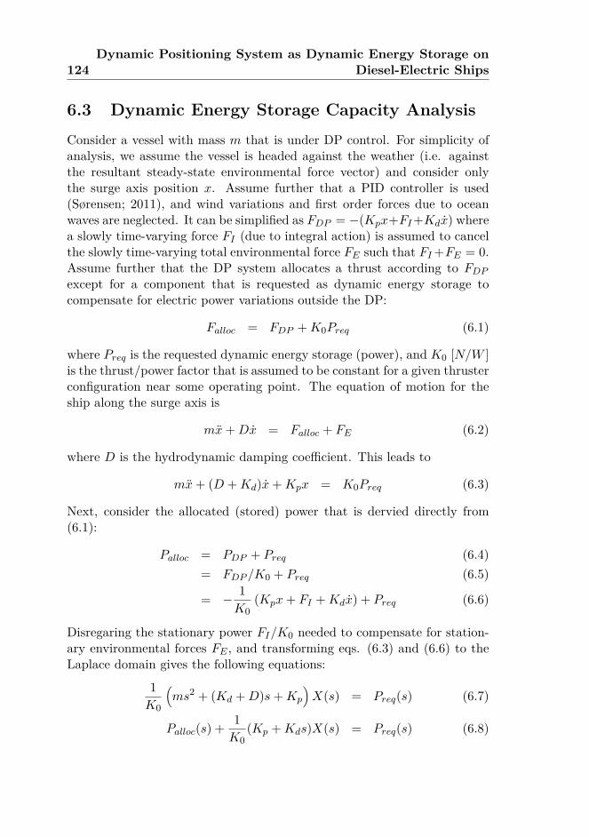
124Dynamic Positioning System as Dynamic Energy Storage on
Diesel-Electric Ships
6.3 Dynamic Energy Storage Capacity AnalysisConsider a vessel with mass m that is under DP control. For simplicity ofanalysis, we assume the vessel is headed against the weather (i.e. againstthe resultant steady-state environmental force vector) and consider onlythe surge axis position x. Assume further that a PID controller is used(Sørensen; 2011), and wind variations and first order forces due to oceanwaves are neglected. It can be simplified as FDP = −(Kpx+FI +Kdx) wherea slowly time-varying force FI (due to integral action) is assumed to cancelthe slowly time-varying total environmental force FE such that FI +FE = 0.Assume further that the DP system allocates a thrust according to FDP
except for a component that is requested as dynamic energy storage tocompensate for electric power variations outside the DP:
Falloc = FDP +K0Preq (6.1)
where Preq is the requested dynamic energy storage (power), and K0 [N/W ]is the thrust/power factor that is assumed to be constant for a given thrusterconfiguration near some operating point. The equation of motion for theship along the surge axis is
mx+Dx = Falloc + FE (6.2)
where D is the hydrodynamic damping coefficient. This leads to
mx+ (D +Kd)x+Kpx = K0Preq (6.3)
Next, consider the allocated (stored) power that is dervied directly from(6.1):
Palloc = PDP + Preq (6.4)= FDP /K0 + Preq (6.5)
= − 1K0
(Kpx+ FI +Kdx) + Preq (6.6)
Disregaring the stationary power FI/K0 needed to compensate for station-ary environmental forces FE , and transforming eqs. (6.3) and (6.6) to theLaplace domain gives the following equations:
1K0
(ms2 + (Kd +D)s+Kp
)X(s) = Preq(s) (6.7)
Palloc(s) + 1K0
(Kp +Kds)X(s) = Preq(s) (6.8)
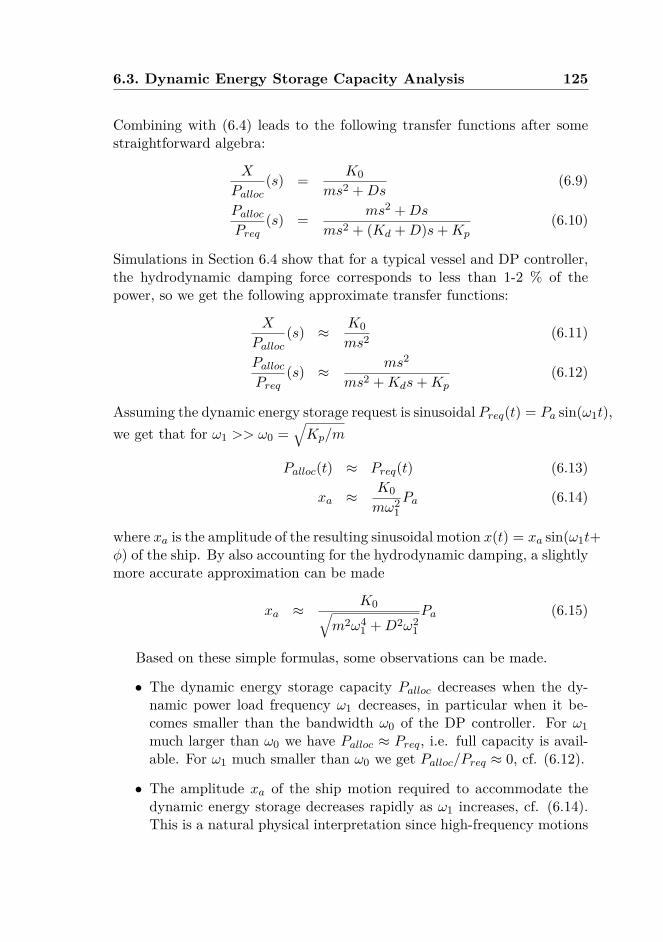
6.3. Dynamic Energy Storage Capacity Analysis 125
Combining with (6.4) leads to the following transfer functions after somestraightforward algebra:
X
Palloc(s) = K0
ms2 +Ds(6.9)
Palloc
Preq(s) = ms2 +Ds
ms2 + (Kd +D)s+Kp(6.10)
Simulations in Section 6.4 show that for a typical vessel and DP controller,the hydrodynamic damping force corresponds to less than 1-2 % of thepower, so we get the following approximate transfer functions:
X
Palloc(s) ≈ K0
ms2 (6.11)
Palloc
Preq(s) ≈ ms2
ms2 +Kds+Kp(6.12)
Assuming the dynamic energy storage request is sinusoidal Preq(t) = Pa sin(ω1t),we get that for ω1 >> ω0 =
√Kp/m
Palloc(t) ≈ Preq(t) (6.13)
xa ≈ K0mω2
1Pa (6.14)
where xa is the amplitude of the resulting sinusoidal motion x(t) = xa sin(ω1t+φ) of the ship. By also accounting for the hydrodynamic damping, a slightlymore accurate approximation can be made
xa ≈ K0√m2ω4
1 +D2ω21
Pa (6.15)
Based on these simple formulas, some observations can be made.
• The dynamic energy storage capacity Palloc decreases when the dy-namic power load frequency ω1 decreases, in particular when it be-comes smaller than the bandwidth ω0 of the DP controller. For ω1much larger than ω0 we have Palloc ≈ Preq, i.e. full capacity is avail-able. For ω1 much smaller than ω0 we get Palloc/Preq ≈ 0, cf. (6.12).
• The amplitude xa of the ship motion required to accommodate thedynamic energy storage decreases rapidly as ω1 increases, cf. (6.14).This is a natural physical interpretation since high-frequency motions
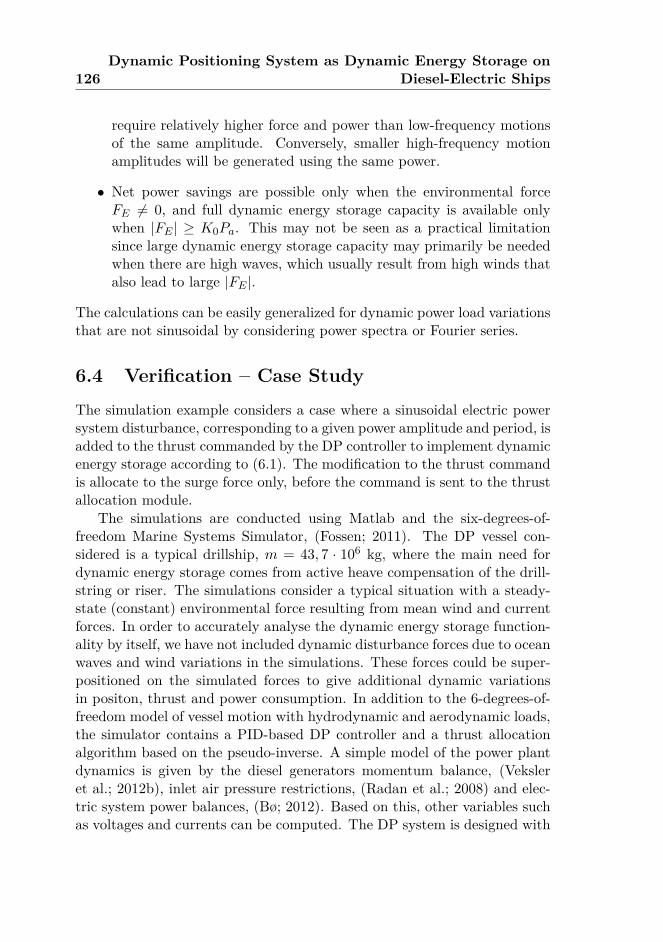
126Dynamic Positioning System as Dynamic Energy Storage on
Diesel-Electric Ships
require relatively higher force and power than low-frequency motionsof the same amplitude. Conversely, smaller high-frequency motionamplitudes will be generated using the same power.
• Net power savings are possible only when the environmental forceFE 6= 0, and full dynamic energy storage capacity is available onlywhen |FE | ≥ K0Pa. This may not be seen as a practical limitationsince large dynamic energy storage capacity may primarily be neededwhen there are high waves, which usually result from high winds thatalso lead to large |FE |.
The calculations can be easily generalized for dynamic power load variationsthat are not sinusoidal by considering power spectra or Fourier series.
6.4 Verification – Case Study
The simulation example considers a case where a sinusoidal electric powersystem disturbance, corresponding to a given power amplitude and period, isadded to the thrust commanded by the DP controller to implement dynamicenergy storage according to (6.1). The modification to the thrust commandis allocate to the surge force only, before the command is sent to the thrustallocation module.
The simulations are conducted using Matlab and the six-degrees-of-freedom Marine Systems Simulator, (Fossen; 2011). The DP vessel con-sidered is a typical drillship, m = 43, 7 · 106 kg, where the main need fordynamic energy storage comes from active heave compensation of the drill-string or riser. The simulations consider a typical situation with a steady-state (constant) environmental force resulting from mean wind and currentforces. In order to accurately analyse the dynamic energy storage function-ality by itself, we have not included dynamic disturbance forces due to oceanwaves and wind variations in the simulations. These forces could be super-positioned on the simulated forces to give additional dynamic variationsin positon, thrust and power consumption. In addition to the 6-degrees-of-freedom model of vessel motion with hydrodynamic and aerodynamic loads,the simulator contains a PID-based DP controller and a thrust allocationalgorithm based on the pseudo-inverse. A simple model of the power plantdynamics is given by the diesel generators momentum balance, (Veksleret al.; 2012b), inlet air pressure restrictions, (Radan et al.; 2008) and elec-tric system power balances, (Bø; 2012). Based on this, other variables suchas voltages and currents can be computed. The DP system is designed with
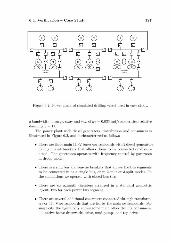
6.4. Verification – Case Study 127
G
M
G
DRILLING DRIVE
G G G G
DRILLING DRIVE
M M M M M
Figure 6.2: Power plant of simulated drilling vessel used in case study.
a bandwidth in surge, sway and yaw of ω0 = 0.033 rad/s and critical relativedamping ζ = 1.0.
The power plant with diesel generators, distribution and consumers isillustrated in Figure 6.2, and is characterized as follows
• There are three main 11 kV buses/switchboards with 2 diesel-generatorshaving circuit breakers that allows them to be connected or discon-neted. The generators operates with frequency-control by governorsin droop mode.
• There is a ring bus and bus-tie breakers that allows the bus segmentsto be connected in as a single bus, or in 2-split or 3-split modes. Inthe simulations we operate with closed bus-ties.
• There are six azimuth thrusters arranged in a standard geometriclayout, two for each power bus segment.
• There are several additional consumers connected through transform-ers or 440 V switchboards that are fed by the main switchboards. Forsimplicity the figure only shows some main other drilling consumers,i.e. active heave drawworks drive, mud pumps and top drive.
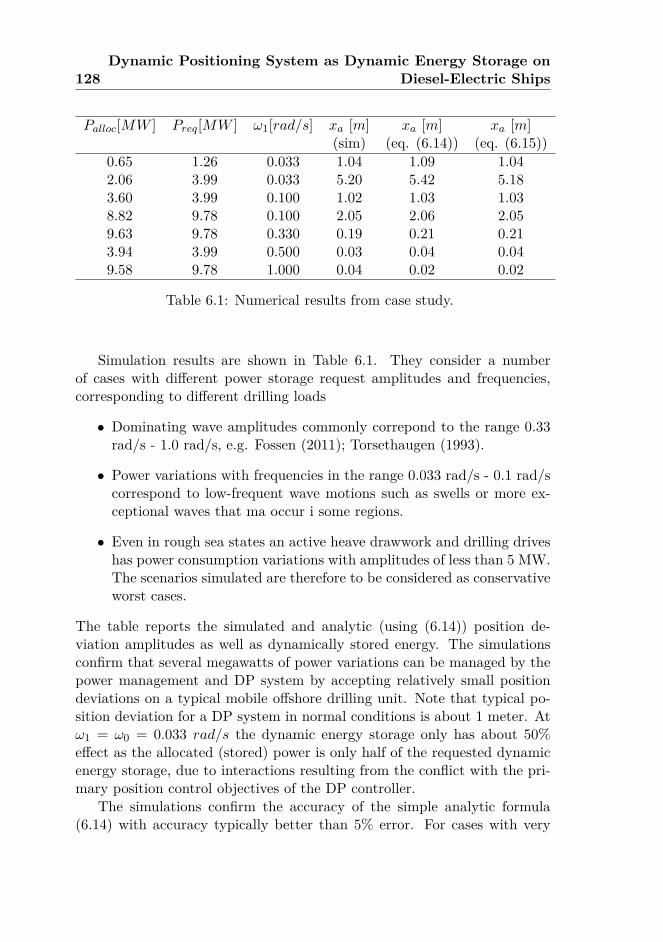
128Dynamic Positioning System as Dynamic Energy Storage on
Diesel-Electric Ships
Palloc[MW ] Preq[MW ] ω1[rad/s] xa [m] xa [m] xa [m](sim) (eq. (6.14)) (eq. (6.15))
0.65 1.26 0.033 1.04 1.09 1.042.06 3.99 0.033 5.20 5.42 5.183.60 3.99 0.100 1.02 1.03 1.038.82 9.78 0.100 2.05 2.06 2.059.63 9.78 0.330 0.19 0.21 0.213.94 3.99 0.500 0.03 0.04 0.049.58 9.78 1.000 0.04 0.02 0.02
Table 6.1: Numerical results from case study.
Simulation results are shown in Table 6.1. They consider a numberof cases with different power storage request amplitudes and frequencies,corresponding to different drilling loads
• Dominating wave amplitudes commonly correpond to the range 0.33rad/s - 1.0 rad/s, e.g. Fossen (2011); Torsethaugen (1993).
• Power variations with frequencies in the range 0.033 rad/s - 0.1 rad/scorrespond to low-frequent wave motions such as swells or more ex-ceptional waves that ma occur i some regions.
• Even in rough sea states an active heave drawwork and drilling driveshas power consumption variations with amplitudes of less than 5 MW.The scenarios simulated are therefore to be considered as conservativeworst cases.
The table reports the simulated and analytic (using (6.14)) position de-viation amplitudes as well as dynamically stored energy. The simulationsconfirm that several megawatts of power variations can be managed by thepower management and DP system by accepting relatively small positiondeviations on a typical mobile offshore drilling unit. Note that typical po-sition deviation for a DP system in normal conditions is about 1 meter. Atω1 = ω0 = 0.033 rad/s the dynamic energy storage only has about 50%effect as the allocated (stored) power is only half of the requested dynamicenergy storage, due to interactions resulting from the conflict with the pri-mary position control objectives of the DP controller.
The simulations confirm the accuracy of the simple analytic formula(6.14) with accuracy typically better than 5% error. For cases with very
6.5. DP Decision Support and Dynamic Consequence Analysis129
small surge amplitudes, the deviation between xa predicted by the simplemodel and the advanced simulation model is relatively large in percent (upto 50%) but negligible in absolute position deviations (a couple of cm). Themain reason why higher relative deviations are observed in these cases is the“higher order” dynamic effects of couplings between surge/pitch (longitudi-nal) and sway/roll (lateral) ship motions included by variations in thrusterforces and moments.
The simulations also verify that the dynamic energy storage has thebenefit that it makes the variations in electric frequency very small (lessthan 1% for all cases) and even less variations in voltage. Moreover, thedynamic energy storage it balances out the difference between consumed andproduced power that results due to the dynamics of the diesel generators.
It has been verified by simulations that the formulas (6.14)-(6.15) qual-itatively are in good agreement also with more advanced implementation ofDP dynamic energy storage, (Veksler et al.; 2012a,b).
6.5 DP Decision Support and Dynamic ConsequenceAnalysis
According to established industry standard system design and operationalprocedures for dynamically positioned ships, (IMO; 1994), it is up to theoperator to enable or disable a sufficient amount of thrusters based on theDP decision support tools such as online consequence analysis, capabilityanalysis, and motion prediction, while the PMS ensures that a sufficientamount of generators are running at all times to serve both operational andpositioning power needs. Conventionally, a redundant number of onlinegenerators and thrusters are employed to guarantee safety and operationalavailability. However, such a redundancy leads to equipment running at lowand inefficient loads, and increases both fuel and maintenance costs as wellas exhaust gas emissions.
By increasing the information exchange and actively taking advantageof the dynamic energy storage capacity offered by the DP system, a less con-servative use of generators and thrusters can be achieved. In particular, thefollowing enhancements can be envisioned within the framework presentedin Figure 6.1, see Bø et al. (2013); Mathiesen et al. (2012) for further details.An online simulation-based dynamic consequence analysis can take into ac-count information about the vessel dynamics, the weather situation (wind,waves and current), load situation, startup time of standby generators andthrusters, etc. to realistically calculate an optimal position reference for
130Dynamic Positioning System as Dynamic Energy Storage on
Diesel-Electric Ships
the DP system which minimizes the chance of drift-off or drive-off whilesimultaneously maximizing the available operational time after generatoror switchboard failure, i.e., how long it is possible to prioritize the opera-tional drives in favor of the thruster drives before safety is compromised.This knowledge can be used to reduce the amount of online generators andthrusters while still achieving operational availability and safety in case ofa failure, sending the information back to PMS system for consumer loadcontrol.
Such integrated and simulation-based power management functionalitycan for instance be employed by drilling vessels, which have flexibility inpositioning depending on the water depth and the corresponding length ofthe drill string. For such vessels, the functionality will ensure that safetywill not be compromised if equipment fails even if a minimum power andthrust configuration is used, because there will be enough time to remedythe failure situation by enabling/disabling relevant power/thrust equipment.Examples include:
• If a generator fails and results in insufficient power, the power con-sumption must be reduced to avoid a blackout. In order to continuethe drilling operation, the thrust consumption must be reduced in-stead of the drilling consumption. Hence, the vessel will experience adrift-off. However, using a simulator-calculated position reference, e.g.Bø et al. (2013), the vessel is already located such that it can safely beallowed to drift for a certain period of time without having to reducethe drilling power consumption in favor of the positioning. Duringthis time frame, the vessel will be able to start the necessary standbygenerators in order to restore sufficient power to stop the drift-off andbring the vessel back into position.
• In the worst case, if the vessel moves close to the safety limit during adrift-off, the power to the operational drives (e.g. drilling drives andmud pumps) must be reduced in favor of power to the thruster drives,in order to maintain the safety of the vessel, equipment and crew.Hence, the integrated system will automatically prioritize drilling ver-sus positioning needs depending on the vessel drift pattern, in orderto continue the drilling operation as long as safely possible.
6.6. Conclusions 131
6.6 ConclusionsSimple formulas are derived in order to related the dynamic energy storagecapacity to the maximum allowed ship position deviation, as a function ofthe frequency of the requested dynamic energy storage. The formulas areverified using a high-fidelity vessel simulator, and show that for dynamicenergy storage requests at wave frequencies (resulting e.g. from an activeheave compensation system) that power variations of several megawatt willresult in position deviations that are no larger than normal position devi-ations resulting from the dynamics of ocean waves and winds, as well asinaccuracies in sensors and position reference systems.
The main advantage of this integrated approach is to maintain opera-tional availability and safety while minimizing power consumption, whichtranslates into lower fuel costs and exhaust gas emissions, as well as min-imizing wear and tear of generators and thrusters, which translates intolower maintenance costs. Relevant applications include marine operationswith positioning flexibility such as drilling.
It could also be mentioned that the method can be directly extendedto other energy storage capacities on-board ships in order to allow morelow-frequency dynamic energy storage requirements, e.g. thermal storagein cooling, cargo, ventilation, air conditioning and other systems. Suchfunctionality is enabled by integrated automation systems that allows therequired software functionality to be implemented.

132Dynamic Positioning System as Dynamic Energy Storage on
Diesel-Electric Ships
Chapter 7
Concluding Remarks
7.1 Conclusion
The motivation behind the thesis was to reduce the environmental footprintof diesel electric propulsion on marine vessels during dynamic positioning.The focus was to reduce the number of diesel engines needed during the oper-ation by modeling and control. The methods presented in the thesis achievethis by either giving support for selection of the optimal configuration, orincreasing the performance of a configuration to fulfill the operational re-quirements. This was achieved by optimizing the power and propulsionsystems as one complete system, and included interaction among subsys-tems. This approach produces a synergistic effect, as shown in Chapters 3and 6, where the inertia of the vessel were used as energy storage duringpower plant recovery and to smooth out power fluctuations.
The power plant designer must be sure that the power plant can fulfillits operational requirements. This means that any single failure on DPvessels of class 2 and 3 should not lead to loss of position. Consequently, itis important that the designer have good tools for testing and verification ofthe vessel’s systems. Otherwise, conservative solutions may be used, whichoften are non-optimal. The simulator in Chapter 2 is a tool for this designprocess. The constraining factor when designing power plants for DP vesselsis often the handling of faults. Since the vessel motion dynamics and powerplant were included in the simulator, new equipment and control strategyfor fault handling can be tested with the simulator. For example were faultrecovery methods using batteries tested with the simulator. Power plantperformance is also affected by interactions between different parts of thevessel, such as the varying power demand due to propeller-wave interactions.
133
134 Concluding Remarks
These effects can be studied with the simulator, and new control methodsfor the plant can be established.
The operator must also be certain that the power plant is configured tofulfill its operational requirements. It is reported from the industry that theoperator often chooses conservative, non-optimal configurations by overrid-ing automatic start/stop of generators and running too many engines. Oneof the reasons for this choice may be lack of relevant information. A dy-namic consequence analysis tool was presented in Chapter 3 to verify DPperformance of the vessel during a fault, so that the operator is certainthat the configuration is safe enough. The operator can check differentconfigurations, such as the number of engines and recovery methods. Thedesired configuration can be selected during or before operations based onthe simulations using this tool.
This thesis also focused on controllers which could make more configu-ration able to fulfill the operation requirements. For example the electricfrequency can drop after some faults in the electric system. Additional en-gines can be committed to avoid a too large frequency drop, which couldlead to blackout. However, this may be unnecessary because the frequencymargin could be increased instead. A scenario-based MPC was presented inChapter 4, which can be used to configure the generators for higher safetymargins or to configure the system so that additional generator sets are notneeded.
Electric frequency variations on the grid due to power variations in de-mand are another challenge that requires the number of engines to be in-creased. These power variations increase fuel consumption and wear andtear. They also make it difficult to synchronize and connect additional gen-erator sets when needed. Control of peak-shaving is presented in Chapter 5,which can be used to reduce these variations in power demand. An MPCwas used in combination with a power spectrum analysis to control peakshaving so that load fluctuations are canceled out as much as possible, whileavoiding too high battery temperatures.
Another method to reduce power fluctuations is to vary power consump-tion of the thrusters, which cancels power fluctuations of other loads. Theeffects of varying power consumption of the thrusters on the DP positionare demonstrated in Chapter 6. An analytical formula is presented, whichgives the size of the position variation as a function of the power variation.The formula was verified with the results from a simulation study.
These methods were simulated using the simulator presented in Chap-ter 2 to verify their performance. The methods presented in this thesis
7.2. Further Work 135
were designed to achieve better control of the vessel’s systems, includingperformance of the DP system and the power plant. These methods canbe used in combination to reduce the number of diesel generators runningwhile maintaining the required safety level or to increase the safety levelthrough better control and information.
7.2 Further Work
The motivation of the thesis was to lower the environmental footprint of ves-sels with diesel electric propulsion and DP. Performance of the controllerswas tested and verified through analytical methods and simulation studies.The next step would be to perform a qualitative study on how much each ofthese methods can reduce emissions from these vessels. This could be accom-plished using the simulator or by full-scale testing. The largest reductionsin emissions are achieved when diesel engine utilization is increased.
The diesel engine model used in this study was a mean value model,which was designed considering steady-state conditions. However, transientperformance was not fully modeled and exhaust gas emissions were notmodeled at all. These models must be developed and validated with full-scale measurements to verify reduced emissions by quantifying the reducedfuel consumption and production of emissions.
This study did not investigate reductions in SOX, NOX, or particulatematter (PM) emissions. However, most of the potential for reduction ofthese emissions is through new equipment and control of the power pro-ducers. Lower SOX, NOX, and PM emissions may also be achieved by thecontrollers described in Chapters 5 and 6, as a smoother power demand mayproduce lower emissions.
Batteries were not a large focus in this study; however, the developmentof batteries has increased rapidly in the last few years. One particularlyinteresting scenario is using batteries as “running stand-by” power supply,since the stand-by cost of a battery is negligible after installation comparedwith diesel engines. Development of such methods would be supported bythe simulator developed in Chapter 2. The dynamic consequence analysisin Chapter 3 is well fitted for operations with DP and batteries, becauseit can be used to estimate plant performance and the minimum batterycharge state. A concept study using batteries as running stand-by shouldbe conducted to determine the increase in performance. This study shouldalso include other power plant changes, such as using diesel engines that areoptimized for slowly varying loads.

136 Concluding Remarks
The simulator models were tested and verified individually. The nextstep is to verify the simulator against full-scale or model-scale measure-ments. Similarly, the controllers and models for the controllers should beverified with full- or model-scale tests to get one step closer to implementa-tion.
Bibliography
ABB (n.d.). Battery-powered ferry - transport with zero emissions, onlinevisited 16-10-2015.URL: http://new.abb.com/marine/articles-and-highlights/battery-powered-ferry—transport-with-zero-emissions
ABS (2014). Guide for dynamic positioning systems. American Bureau ofShipping.
Altosole, M., Benvenuto, G., Figari, M. and Campora, U. (2009). Real-timesimulation of a COGAG naval ship propulsion system, Proceedings of theInstitution of Mechanical Engineers, Part M: Journal of Engineering forthe Maritime Environment 223: 47–62.
Angeli, D., Amrit, R. and Rawlings, J. B. (2012). On average performanceand stability of economic model predictive control, IEEE Trans. Automat.Contr. 57(7): 1615–1626.
Bazari, Z. and Longva, T. (2011). Assessment of IMO mandated energyefficiency measures for international shipping, Technical Report MEPC63/INF.2, Lloyd’s Register and DNV.
Bemporad, A., Bellucci, L. and Gabbriellini, T. (2014). Dynamic optionhedging via stochastic model predictive control based on scenario simu-lation, Quantitative Finance pp. 1739–1751.
Benajes, J., Luján, J. M., Bermúdez, V. and Serrano, J. R. (2002). Mod-elling of turbocharged diesel engines in transient operation. Part 1: In-sight into the relevant physical phenomena, Proceedings of the Institu-tion of Mechanical Engineers, Part D: Journal of Automobile Engineering216(5): 431–441.
137
138 Bibliography
Bernardini, D. and Bemporad, A. (2009). Scenario-based model predic-tive control of stochastic constrained linear systems, Decision and Con-trol, 2009 held jointly with the 2009 28th Chinese Control Conference.CDC/CCC 2009. Proceedings of the 48th IEEE Conference on, pp. 6333–6338.
Blanke, M., Kinnaert, M., Lunze, J. and Staroswiecki, M. (2006). Diagnosisand Fault-Tolerant Control, Diagnosis Fault-Tolerant Control, 2nd edn,Springer Berlin Heidelberg, pp. 10–23.
Bonfill, A., Espuña, A. and Puigjaner, L. (2008). Proactive approach toaddress the uncertainty in short-term scheduling, Computers & chemicalengineering 32(8): 1689–1706.
Bosich, D., Filippo, M., Giulivo, D., Sulligoi, G. and Tessarolo, A. (2012).Thruster motor start-up transient in an all-electric cruise-liner: Numericalsimulation and experimental assessment, Electrical Systems for Aircraft,Railway and Ship Propulsion (ESARS), 2012, pp. 1–5.
Bravo, J. M., Alamo, T. and Camacho, E. F. (2006). Robust MPC of con-strained discrete-time nonlinear systems based on approximated reachablesets, Automatica 42(10): 1745–1751.
Brown, R. G. and Hwang, P. Y. (1997). Introduction to Random Signalsand Applied Kalman Filtering, third edn, Wiley.
Bø, T. I. (2012). Dynamic model predictive control for load sharing inelectric power plants for ships, Master’s thesis, Norwegian University ofScience and Technology.
Bø, T. I., Dahl, A. R., Johansen, T. A., Mathiesen, E., Miyazaki, M. R.,Pedersen, E., Skjetne, R., Sørensen, A. J., Thorat, L. and Yum, K. K.(2015). Marine vessel and power plant system simulator, IEEE Access3: 2065–2079.
Bø, T. I. and Johansen, T. A. (2013). Scenario-based fault-tolerant modelpredictive control for diesel-electric marine power plant, MTS/IEEEOcean., Bergen, Norway.
Bø, T. I. and Johansen, T. A. (2014). Dynamic safety constraints by scenariobased economic model predictive control, Proc. IFAC World Congress,Cape Town, South Africa, pp. 9412–9418.
Bibliography 139
Bø, T. I. and Johansen, T. A. (n.d.a). Battery peak-shaving control in elec-tric marine power plant using nonlinear model predictive control. Sub-mitted for publication.
Bø, T. I. and Johansen, T. A. (n.d.b). Dynamic safety constraints byscenario-based economic model predictive control. Submitted for pub-lication.
Bø, T. I., Johansen, T. A. and Mathiesen, E. (2013). Unit Commitment ofGenerator Sets During Dynamic Positioning Operation Based on Conse-quence Simulation, Proc. 9th IFAC Conf. Control Applications in MarineSystems, Osaka, Japan.
Bø, T. I., Johansen, T. A., Sørensen, A. J. and Mathiesen, E. (n.d.). Dy-namic consequence analysis of marine electric power plant in dynamicpositioning. Submitted for publication.
Calafiore, G. C. and Fagiano, L. (2013). Robust Model Predictive Controlvia Scenario Optimization, IEEE Trans. Automat. Contr. 58(1): 219–224.
Chase, M. W. (1998). NIST-JANAF thermochemical tables, Vol. no. 9,American Chemical Society and the American Institute of Physics forthe National Institute of Standards and Technology, Washington, D.C.
Chen, W., Ådnanes, A., Hansen, J., Lindtjørn, J. and Tang, T. (2010).Super-capacitors based hybrid converter in marine electric propulsion sys-tem, Electrical Machines (ICEM), 2010 XIX International Conference on,pp. 1–6.
Chow, A. and Wyszynski, M. L. (1999). Thermodynamic modelling of com-plete engine systems—a review, Proceedings of the Institution of Mechan-ical Engineers, Part D: Journal of Automobile Engineering 213(4): 403–415.
Contaxis, G. C. and Kabouris, J. (1991). Short term scheduling in awind/diesel autonomous energy system, IEEE Transactions on PowerSystems 6(3): 1161–1167.
Coogan, S. and Arcak, M. (2012). Guard synthesis for safety of hybrid sys-tems using sum of squares programming, 51st IEEE Conf. Decis. Control,pp. 6138–6143.
140 Bibliography
Dillon, T. S., Edwin, K. W., Kochs, H. D. and Taud, R. J. (1978). Inte-ger programming approach to the problem of optimal unit commitmentwith probabilistic reserve determination, IEEE Transactions on PowerApparatus and Systems PAS-97(6): 2154–2166.
DNV (2010). Dynamic positioning system - enhanced reliability DYNPOS-ER, Technical Report Rules for classification of ships, Part 6, Chapter26.
DNV (2012). Failure mode and effect analysis (FMEA) of redundant sys-tems. Det Norske Veritas.
DNV (2015). Rules for Classification of Ships. Det Norske Veritas, July.
DNV GL (2015a). Offshore technical guide 10, DP-classed vessels withclosed bus-tie(s), Technical report.
DNV GL (2015b). Rules for Classification of Ships. DNV GL. October.
DNV GL (n.d.). Sesam marine. Viewed 17-10-2015.www.dnvgl.com/services/software-for-marine-operations-sesam-marine-2321.
Dokopoulos, P. S. and Saramourtsis, A. C. (1996). Prediction and Evalua-tion of the Performance of Wind-Diesel Energy Systems, IEEE Transac-tions on Energy Conversion 11(2): 385–393.
Ehsani, M., Gao, Y. and Emadi, A. (2009). Modern electric, hybrid electric,and fuel cell vehicles: fundamentals, theory, and design, CRC press.
Eidsvik (2015). Viking Queen installation of energy storage system.Accessed: 2015-08-27.URL: www.eidesvik.no/news-archive/viking-queen-installation-of-energy-storage-system-article645-299.html
Eriksen, P. B. and Orths, A. (2008). From 20 to 50 percent of wind energyin the danish power system, Keynote presentation at 7th internationalworkshop of large-scale integration of wind power and on transmissionnetworks for offshore wind farms; 26–28 May 2008. Madrid, Spain.
Faltinsen, O. M. (1990). Sea Loads on Ships and Offshore Structures, Cam-bridge University Press.
Bibliography 141
Fossen, T. I. (2002). Marine Control Systems: Guidance, Navigation andControl of Ships, Rigs and Underwater Vehicles, Marine Cybernetics,Trondheim, Norway.
Fossen, T. I. (2011). Handbook of Marine Craft Hydrodynamics and MotionControl, John Wiley and sons.
Fossen, T. I. and Strand, J. P. (1999). Passive nonlinear observer designfor ships using lyapunov methods: full-scale experiments with a supplyvessel, Automatica 35(1): 3 – 16.
Gillula, J. H., Hoffmann, G. M., Vitus, M. P. and Tomlin, C. J. (2011).Applications of hybrid reachability analysis to robotic aerial vehicles, TheInternational Journal of Robotics Research 30(3): 335–354.
Goodwin, G. C. and Medioli, A. M. (2013). Scenario-based, closed-loopmodel predictive control with application to emergency vehicle scheduling,International Journal of Control 86(8): 1338–1348.
Grüne, L. (2013). Economic receding horizon control without terminal con-straints, Automatica 49(3): 725–734.
Guzzella, L. and Onder, C. H. (2010). Introduction to Modeling and Con-trol of Internal Combustion Engine Systems, second edn, Springer BerlinHeidelberg, Berlin, Heidelberg.
Hansen, J. F., Ådnanes, A. K. and Fossen, T. I. (1998). Modelling, simu-lation and multivariable modelbased predictive control of marine powergeneration system, Proceedings of IFAC Conference: Control Applicationsin Marine Systems, CAMS’98, Fukuoka, Japan, pp. 45–50.
Hansen, J. F., Ådnanes, A. K. and Fossen, T. I. (2001). Mathematicalmodelling of diesel-electric propulsion systems for marine vessels, Mathe-matical and Computer Modelling of Dynamical Systems 7(3): 323–355.
Hansen, J. F. and Fossen, T. I. (1999). Nonlinear control of marine powergeneration systems, Proc. of 13th Power Systems Computation Confer-ence, Trondheim, Norway, pp. 539–544.
Hansen, J. F., Lindtjørn, J. O. and Vänskä, K. (2011). Onboard DC grid forenhanced DP operation in ships, Dynamic Positioning Conference, MTS,Houston, USA.
142 Bibliography
Hansen, J. F. and Wendt, F. (2015). History and State of the Art in Com-mercial Electric Ship Propulsion, Integrated Power Systems, and FutureTrends, Proceedings of the IEEE 103(12): 2229–2242.
Hanssen, K. G., Foss, B. and Teixeira, A. (2015). Production optimiza-tion under uncertainty with constraint handling, 2nd IFAC Workshop onAutomatic Control in Offshore Oil and Gas Production, pp. 62–67.
Hasselmann, K., Barnett, T., Bouws, E., Carlson, H., Cartwright, D., Enke,K., Ewing, J., Gienapp, H., Hasselmann, D., Kruseman, P. et al. (1973).Measurements of wind-wave growth and swell decay during the joint northsea wave project (JONSWAP), Technical report, Deutches Hydrographis-ches Institut.
Hermance, D. and Sasaki, S. (1998). Hybrid electric vehicles take to thestreets, Spectrum, IEEE 35(11): 48–52.
Heywood, J. B. (1988). Internal Combustion Engine Fundamentals, Mc-Graw Hill.
Holttinen, H., Meibom, P., Orths, A., Lange, B., O’Malley, M., Tande, J. O.,Estanqueiro, A., Gomez, E., Söder, L., Strbac, G., Smith, J. C. and vanHulle, F. (2011). Impacts of large amounts of wind power on design andoperation of power systems, results of IEA collaboration, Wind Energy14(2): 179–192.
Houska, B., Ferreau, H. J. and Diehl, M. (2011). ACADO toolkit — anopen-source framework for automatic control and dynamic optimization,Optimal Control Applications and Methods 32(3): 298–312.
Hovgaard, T. G., Larsen, L. F. S., Jørgensen, J. B. and Boyd, S. (2013).MPC for wind power gradients — utilizing forecast, rotor inertia, andcentral energy storage, European Control Conference, Zürich, Switzer-land, pp. 4071–4076.
Hovgaard, T., Larsen, L. and Jørgensen, J. (2011). Robust economic mpc fora power management scenario with uncertainties, Decision and Controland European Control Conference (CDC-ECC), 2011 50th IEEE Confer-ence on, pp. 1515–1520.
Huhman, B. M. and Wetz, D. A. (2015). Progress in the Development of aBattery-based Pulsed Power System, Electric Ship Technologies Sympo-sium (ESTS), 2015 IEEE, pp. 441–445.
Bibliography 143
Huria, T., Ceraolo, M., Gazzarri, J. and Jackey, R. (2012). High fidelityelectrical model with thermal dependence for characterization and sim-ulation of high power lithium battery cells, Electric Vehicle Conference(IEVC), 2012 IEEE International, pp. 1–8.
IMCA (1995–2011). Dynamic positioning station keeping incidents, Tech-nical report, International Marine Contractors Association.
IMCA (2000). Specification for DP capability plots, Technical Report IMCAM140, The International Marine Contractors Association. Revision 1.
IMO (1994). Guidelines for vessels with dynamic positioning systems, Tech-nical Report Maritime Safety Committee (MSC) Circular 645, Interna-tional Maritime Organization (IMO).
IMO (2011). International convention for the prevention of pollution fromships (MARPOL) Annex VI. International Maritime Organization (IMO).
ISO (2009). ISO 13624-1:2009 Petroleum and natural gas industries –Drilling and production equipment – Part 1: Design and operation ofmarine drilling riser equipment. International Organization for Standard-ization.
Jenssen, N. A. and Realfsen, B. (2006). Power optimal thruster allocation,Proc. Dynamic Positioning Conference, Houston.
Johansen, T. A., Bø, T. I., Mathiesen, E., Veksler, A. and Sørensen, A. J.(2014). Dynamic positioning system as dynamic energy storage on diesel-electric ships, Power Systems, IEEE Transactions on 29(6): 3086–3091.
Johansen, T. A. and Sørensen, A. J. (2009). Experiences with hil simulatortesting of power management systems, Dynamic Positioning Conference,Marine Technology Society, Houston, USA.
Johnson, V. H., Wipke, K. B. and Rausen, D. J. (2000). HEV control strat-egy for real-time optimization of fuel economy and emissions, Technicalreport, SAE Technical Paper.
Juste, K. A., Kita, H., Tanaka, E. and Hasegawa, J. (1999). An evolu-tionary programming solution to the unit commitment problem, IEEETransactions on Power Systems 14(4): 1452–1459.
144 Bibliography
Kim, I.-S. (2008). Nonlinear state of charge estimator for hybrid electricvehicle battery, Power Electronics, IEEE Transactions on 23(4): 2027–2034.
Kim, S.-Y., Choe, S., Ko, S. and Sul, S.-K. (2015). A naval integrated powersystem with a battery energy storage system: Fuel efficiency, reliability,and quality of power., Electrification Magazine, IEEE 3(2): 22–33.
Kongsberg Maritime (n.d.). K-POS, online, view 22-10-2015.URL: www.km.kongsberg.com/ks/web/nokbg0397.nsf/AllWeb/23EE29C2A5B1E771C12571CA004B3827/$file/k-pos-brochure.pdf?OpenElement
Kottick, D., Blau, M. and Edelstein, D. (1993). Battery energy storagefor frequency regulation in an island power system, Energy Conversion,IEEE Transactions on 8(3): 455–459.
Kovâcshâzy, T., Péceli, G. and Simon, G. (2001). Transient reduction inreconfigurable control systems utilizing structure dependence, Instrumen-tation and Measurement Technology Conference, 2001. IMTC 2001. Pro-ceedings of the 18th IEEE, pp. 1143–1147.
Krause, P. C., Wasynczuk, O. and Sudhoff, S. D. (2013). Analysis of ElectricMachinery and Drive Systems, 3 edn, McGraw Hill Higher Education.
Kristiansen, S. (2014). Analysis of loss of position incidents for dynamicallyoperated vessels, Master’s thesis, Norwegian University of Science andTechnology.
Kuznetsov, S. (2015). Large Scale Energy Storage Module for Surface Com-batants : Transmission and System Transient Characteristics, Electr. Sh.Technol. Symp. (ESTS), 2015 IEEE, pp. 167–172.
Lao, L., Ellis, M. and Christofides, P. D. (2013). Proactive Fault-TolerantModel Predictive Control, AIChE J. 59(8): 2810–2820.
Lee, C.-H. (1995). WAMIT Theory Manual, Massachusettes Institute ofTechnology.URL: http://www.wamit.com/Publications/tmanual.pdf
Levron, Y., Guerrero, J. and Beck, Y. (2013). Optimal power flow inmicrogrids with energy storage, IEEE Transactions on Power Systems28(3): 3226–3234.
Bibliography 145
Levron, Y. and Shmilovitz, D. (2012). Power systems’ optimal peak-shavingapplying secondary storage, Electric Power Systems Research 89(0): 80 –84.
Limon, D., Alamo, T., Raimondo, D. M., Peña, D. M. n., Bravo, J. M., Fer-ramosca, A. and Camacho, E. F. (2009). Input-to-state stability: a uni-fying framework for robust model predictive control, in L. Magni, D. M.Raimondo and F. Allgöwer (eds), Nonlinear Model Predict. Control, Vol.384, Springer Berlin Heidelberg, pp. 1–26.
Lin, C.-C., Peng, H., Grizzle, J. W. and Kang, J.-M. (2003). Power man-agement strategy for a parallel hybrid electric truck, Control SystemsTechnology, IEEE Transactions on 11(6): 839–849.
Lowery, P. G. (1966). Generating unit commitment by dynamic pro-gramming, IEEE Transactions on Power Apparatus and Systems PAS-85(5): 422–426.
Maciejowski, J. M. (2002). Predictive Control with Constraints, PearsonEucation.
Maiworm, M., Bäthge, T. and Findeisen, R. (2015). Scenario-based modelpredictive control: Recursive feasibility and stability, Proc. of 9th IFACSymposium on Advanced Control of Chemical Processes ADCHEM 2015,Vol. 48, Whistler, Canada, pp. 50 – 56.
MAN Engines and Systems (2013). 32/44CR Project Guide - Marine.URL: marine.man.eu/four-stroke/project-guides
Marine Cybernetics (n.d.). Technology: Cybersea. Viewed 2014-12-12.marinecybernetics.com/technology/cybersea.
Marine Environment Protection Committee, IMO (2014). Third IMO GHGstudy 2014, Technical report, International Maritime Organization (IMO).
Martini, F. (2015). First electrical car ferry in the world in operation inNorway now, Siemens, Pictures of the Future.
Mathiesen, E., Realfsen, B. and Breivik, M. (2012). Methods for reduc-ing frequency and voltage variations on DP vessels, Dynamic PositioningConference, Marine Technology Society, Houston, USA.
146 Bibliography
Matusko, J. and Borrelli, F. (2012). Scenario-based approach to stochasticlinear predictive control, Decision and Control (CDC), 2012 IEEE 51stAnnual Conference on, pp. 5194–5199.
May, J. J. (2003). Improving engine utilization on DP drilling vessels,Dynamic Positioning Conference, Marine Technology Society, Houston,USA.
May, J. J. and Foss, H. (2000). Power Management System for the “Deep-water Horizon” a dynamically positioned all weather semisubmersible,Dynamic Positioning Conference, Marine Technology Society, Houston,USA.
Mayne, D. Q., Rawlings, J. B., Rao, C. V. and Scokaert, P. O. M. (2000).Constrained model predictive control: Stability and optimality, Automat-ica 36(6): 789–814.
Miniovich, I. Y. (1960). Investigation of Hydrodynamic Characteristics ofScrew Propellers Under Conditions of Reversing and Calculation Methodsfor Backing of Ships.
Moura, S. J., Fathy, H. K., Callaway, D. S. and Stein, J. L. (2011). Astochastic optimal control approach for power management in plug-inhybrid electric vehicles, Control Systems Technology, IEEE Transactionson 19(3): 545–555.
MSS (2010). Marine systems simulator. marinecontrol.org.
Myklebust, T. A. and Ådnanes, A. K. (n.d.). Parallel hybrid propulsion forAHTS, online, viewed 01.10.2015.URL: https://library.e.abb.com/public/d4355c6a83641884c1257a8a003c5ada/ABB%20Generations_24%20Parallel%20hybrid%20propulsion%20for%20AHTS.pdf
Oldewurtel, F., Parisio, A., Jones, C. N., Morari, M., Gyalistras, D., Gw-erder, M., Stauch, V., Lehmann, B. and Wirth, K. (2010). Energy ef-ficient building climate control using stochastic model predictive con-trol and weather predictions, American Control Conference (ACC), 2010,pp. 5100–5105.
Opsand, S. (2015). Maritime battery forum, Presentation at Electric &Hybrid Marine World Expo 2015.
Bibliography 147
Overbye, S. (1989). Fra forskning til industri, utvikling av skipsautomatis-eringsbedriften norcontrol, Master’s thesis, University of Oslo, Norway.
Pachauri, R. K., Allen, M. R., Barros, V. R., Broome, J., Cramer, W.,Christ, R., Church, J. A., Clarke, L., Dahe, Q., Dasgupta, P., Dubash,N. K., Edenhofer, O., Elgizouli, I., Field, C. B., Forster, P., Friedling-stein, P., Fuglestvedt, J., Gomez-Echeverri, L., Hallegatte, S., Hegerl, G.,Howden, M., Jiang, K., Cisneroz, B. J., Kattsov, V., Lee, H., Mach, K. J.,Marotzke, J., Mastrandrea, M. D., Meyer, L., Minx, J., Mulugetta, Y.,O’Brien, K., Oppenheimer, M., Pereira, J. J., Pichs-Madruga, R., Plat-tner, G.-K., Pörtner, H.-O., Power, S. B., Preston, B., Ravindranath,N. H., Reisinger, A., Riahi, K., Rusticucci, M., Scholes, R., Seyboth, K.,Sokona, Y., Stavins, R., Stocker, T. F., Tschakert, P., van Vuuren, D.and van Ypserle, J.-P. (2014). Climate Change 2014: Synthesis Report.Contribution of Working Groups I, II and III to the Fifth Assessment Re-port of the Intergovernmental Panel on Climate Change, IPCC, Geneva,Switzerland.
Paran, S., Vu, T., El Mezyani, T. and Edrington, C. (2015). MPC-basedpower management in the shipboard power system, Electric Ship Tech-nologies Symposium (ESTS), 2015 IEEE, pp. 14–18.
Park, H., Sun, J., Pekarek, S., Stone, P., Opila, D., Meyer, R., Kolmanovsky,I. and DeCarlo, R. (2015). Real-time model predictive control for ship-board power management using the IPA-SQP approach, Control SystemsTechnology, IEEE Transactions on 23(6): 2129–2143.
Pascoal, R., Guedes Soares, C. and Sørensen, A. J. (2007). Ocean wave spec-tral estimation using vessel wave frequency motions, Journal of OffshoreMechanics and Arctic Engineering 129(2): 90–96.
Pedersen, E. and Engja, H. (2000). A Bond Graph Model Library for Mod-elling Diesel Engine Transient Performance, ISME Tokyo 2000, Vol. 2,Tokyo, pp. 447–455.
Pedersen, T. A. and Pedersen, E. (2012). Bond graph modelling of ma-rine power systems, Mathematical and Computer Modelling of DynamicalSystems 18(2): 153–173.
Perez, T. and Blanke, M. (2003). DCMV a MATLAB/Simulink toolboxfor dynamics and control of marine vehicles, 6th IFAC MCMC, Girona,Spain.
148 Bibliography
Perez, T., Smogeli, Ø. N., Fossen, T. I. and Sørensen, A. J. (2006). AnOverview of the Marine Systems Simulator (MSS): A Simulink Tool-box for Marine Control Systems, Modeling, Identification and Control27(4): 259–275.
Piller, S., Perrin, M. and Jossen, A. (2001). Methods for state-of-charge de-termination and their applications, Journal of Power Sources 96(1): 113– 120. Proceedings of the 22nd International Power Sources Symposium.
Pivano, L., Muddusetti, S. and Ramsey, J. (2014). Better analysis - betterdata - better decisions - better operational risk management = deliveryof incident free operations: Enabled by DynCap, Dynamic PositioningConference, Marine Technology Society, Houston, USA.
Plett, G. L. (2004). Extended kalman filtering for battery managementsystems of LiPB-based HEV battery packs: Part 3. state and parameterestimation, Journal of Power Sources 134(2): 277 – 292.
Prajna, S., Jadbabaie, A. and Pappas, G. J. (2007). A Framework forWorst-Case and Stochastic Safety Verification Using Barrier Certificates,IEEE Trans. Automat. Contr. 52(8): 1415–1428.
Qin, S. J. and Badgwell, T. A. (2003). A survey of industrial model predic-tive control technology, Control Engineering Practice 11(7): 733 – 764.
Radan, D. (2008). Integrated Control of Marine Electrical Power Systems,Doctoral thesis, monograph, Department of Marine Technology, Facultyof Engineering Science & Technology, NTNU.
Radan, D., Johansen, T. A., Sørensen, A. J. and Ådnanes, A. K. (2005).Optimization of load dependent start tables in marine power managementsystems with blackout prevention, WSEAS Transactions on Circuits andSystems 4(12): 1861–1866.
Radan, D., Sørensen, A. J., Ådnanes, A. K. and Johansen, T. A. (2008).Reducing power load fluctuations on ships using power redistribution con-trol, Marine Technology 45(3): 162–174.
Radan, D., Sørensen, A. J., Johansen, T. A. and Ådnanes, A. K. (2006).Probability based generator commitment optimization in ship power sys-tem design., WSEAS Transactions on Systems 5(8): 1901–1906.
Bibliography 149
Rawlings, J. B. and Muske, K. R. (1993). The stability of constrainedreceding horizon control, IEEE Trans. Automat. Contr. 38(10): 1512–1516.
Realfsen, B. (2009). Reducing NOx Emission in DP2 and DP3 Operations,Dynamic Positioning Conference, Marine Technology Society, Houston,USA.
Ren, W., Steurer, M. and Woodruff, S. (2005). Progress and challenges inreal time hardware-in-the loop simulations of integrated ship power sys-tems, Power Engineering Society General Meeting, 2005. IEEE, pp. 534–537 Vol. 1.
Schildbach, G., Fagiano, L., Frei, C. and Morari, M. (2014). The scenarioapproach for stochastic model predictive control with bounds on closed-loop constraint violations, Automatica 50(12): 3009–3018.
Scokaert, P. O. M. and Mayne, D. Q. (1998). Min-max feedback modelpredictive control for constrained linear systems, IEEE Trans. Automat.Contr. 43(8): 1136–1142.
Sebastián, R. and Quesada, J. (2006). Distributed control system for fre-quency control in a isolated wind system, Renewable Energy 31(3): 285 –305.
Senjyu, T. and Shimabukuro, K. (2003). A fast technique for unit com-mitment problem by extended priority list, IEEE Trans. Power Syst.18(2): 882–888.
Shi, X., Wei, Y., Ning, J., Fu, M. and Zhao, D. (2011). Optimizing adap-tive thrust allocation based on group biasing method for ship dynamicpositioning, Automation and Logistics (ICAL), 2011 IEEE InternationalConference on, pp. 394–398.
Skjetne, R. (2010). Modeling a diesel-generator power plant. Lecture notes,Norwegian University of Science and Technology.
Skjong, E., Molinas, M. and Johansen, T. A. (2015). Optimized currentreference generation for system-level harmonic mitigation in a diesel-electric ship using non-linear model predictive control, Industrial Tech-nology (ICIT), 2015 IEEE International Conference on, pp. 2314–2321.
150 Bibliography
Skjong, E., Molinas, M., Johansen, T. A. and Volden, R. (2015). Shapingthe current waveform of an active filter for optimized system level har-monic conditioning, International Conference on Vehicle Technology andIntelligent Transport Systems, Lisbon, Portugal.
Skjong, E., Ochoa-Gimenez, M., Molinas, M. and Johansen, T. A. (2015).Management of harmonic propagation in a marine vessel by use of opti-mization, Proc. IEEE Transportation Electrification Conference and Expo(ITEC 2015), Detroit, USA.
Skjong, E., Rødskar, E., Molinas, M., Johansen, T. A. and Cunningham,J. (2015). The marine vessel’s electrical power system: From its birth topresent day, Proceedings of the IEEE 103(12).
Smogeli, Ø. N. (2006). Control of Marine Propellers, PhD thesis, Depart-ment of Marine Technology, Faculty of Engineering Science & Technology,NTNU.
Steurer, M., Andrus, M., Langston, J., Qi, L., Suryanarayanan, S.,Woodruff, S. and Ribeiro, P. (2007). Investigating the impact of pulsedpower charging demands on shipboard power quality, Electric Ship Tech-nologies Symposium, 2007. ESTS ’07. IEEE, pp. 315–321.
Stone, P., Opila, D., Park, H., Sun, J., Pekarek, S., DeCarlo, R., Westervelt,E., Brooks, J. and Seenumani, G. (2015). Shipboard power managementusing constrained nonlinear model predictive control, Electric Ship Tech-nologies Symposium (ESTS), 2015 IEEE, pp. 1–7.
Sørensen, A. J. (2011). A survey of dynamic positioning control systems,IFAC Journal of Annual Reviews in Control 35(1): 123 – 136.
Sørensen, A. J. (2013). Marine Control Systems: Propulsion and MotionControl Systems of Ships and Ocean Structures., second edn, Dep. ofMarine Technology, NTNU.
Sørensen, A. J., Pedersen, E. and Smogeli, Ø. N. (2003). Simulation-baseddesign and testing of dynamically positioned marine vessels, InternationalConference on Marine Simulation and Ship Maneuverability (MARSIM),Japan.
Sørensen, A. J. and Smogeli, Ø. N. (2009). Torque and power control ofelectrically driven marine propellers, Control Eng. Pract. 17(9): 1053–1064.
Bibliography 151
Torrisi, F. D. and Bemporad, A. (2001). Discrete-time hybrid modeling andverification, IEEE Conf. Decis. Control, pp. 2899–2904.
Torsethaugen, K. (1993). A two peak wave spectrum model, Proc. 12th Int.Conf. Offshore Mechanics and Arctic Technolog, Vol. 2, pp. 175–180.
Vada, J., Slupphaug, O. and Johansen, T. A. (2001). Optimal prioritizedinfeasibility handling in model predictive control: parametric preemp-tive multiobjective linear programming approach, Journal of Optimiza-tion Theory and Applications 109(2): 385–413.
Valmot, O. R. (2014). Norske batterier kan levere 54 kWh på seks minutter,Teknisk Ukeblad .URL: http://www.tu.no/industri/2014/12/19/ norske-batterier-kan-levere-54-kwh-pa-seks-minutter
Veksler, A., Johansen, T. A., Mathiesen, E. and Skjetne, R. (2013). Gover-nor principles for increased safety on vessels with diesel-electric propul-sion, European Control Conference, Zurich, Switzerland, pp. 2579–2584.
Veksler, A., Johansen, T. A. and Skjetne, R. (2012a). Thrust allocationwith power management functionality on dynamically positioned vessels,Proc. American Control Conference, Monteal.
Veksler, A., Johansen, T. A. and Skjetne, R. (2012b). Transient power con-trol in dynamic positioning — governor feedforward and dynamic thrustallocation, IFAC conference on maneuvering and control of marine craft.,Arenzano, Italy.
Weisser, D. and Garcia, R. S. (2005). Instantaneous wind energy penetra-tion in isolated electricity grids: concepts and review, Renewable Energy30(8): 1299 – 1308.
Wirasingha, S. and Emadi, A. (2011). Classification and review of controlstrategies for plug-in hybrid electric vehicles, Vehicular Technology, IEEETransactions on 60(1): 111–122.
Woodward (2004). Governing Fundamentals and Power Management.Viewed 2014-12-15.URL: woodward.com/workarea/downloadasset.aspx?id=2147483987
Xie, Y., Sun, J., Miz, C. and Freudenberg, J. (2009). Analysis and modelingof a DC hybrid power system testbed for power management strategy
152 Bibliography
development, Vehicle Power and Propulsion Conference, 2009. VPPC’09.IEEE, IEEE, pp. 926–933.
Yum, K. K. and Pedersen, E. (2013). Transient performance and emissionprediction of diesel engine system using pseudo bond graph model, The9th Asia-Pacific Conference on Combustion, Gyeongju, Korea.
Zacharias, F. (1967). Analytical Representation of the ThermodynamicProperties of Combustion Gases, SAE Technical Paper 670930.
Zahedi, B. and Norum, L. (2013). Modeling and simulation of all-electricships with low-voltage DC hybrid power systems, IEEE Transactions onPower Electronics 28(10): 4525–4537.
Zeng, J., Zhang, B., Mao, C. and Wang, Y. (2006). Use of battery en-ergy storage system to improve the power quality and stability of windfarms, Power System Technology, 2006. PowerCon 2006. InternationalConference on, pp. 1–6.
Ådnanes, A. K. (2003). Maritime Electrical Installations and Diesel ElectricPropulsion, Oslo, Norway.