ROBINSONWorking Paper No. 08-08

Towards Taming the New Consensus :Hysteresis and Some Other Post-Keynesian

Amendments

by

Marc LavoieMarc.Lavoie@uottawa.ca

May 2008

Research On Banking International and National Systems Or NetworksUniversity of Ottawa, 200 Wilbrod Street, Ottawa, ON, KlN 6N5, Canada

http://aix1.uottawa.ca/~robinson

1. Introduction

Not so long ago, most economists believed that central banks ought to set money supply targets, implementing these targets by controlling the supply of base money. The New Consensus among central bankers and economists active in the field of monetary economics is now that central banks ought to set target nominal interest rates, thus controlling real interest rates and influencing output and inflation rates. Still, in the 1960s and 1970s, those academics who argued that central banks could not control the supply of money and had to implement monetary policy through interest rate targeting were ridiculed. Their views were considered sterile and dépassées.

Part of the New Consensus is now the eclectic view that money supply control is preferable when the real side in macroeconomics is more volatile than the monetary side, while interest rate targeting is better when the monetary side – the demand for money – is more volatile. Authors of all stripes rely on Poole (1970) for this insight. In other words, if we could just go back to a world where financial innovations would vanish or be predicted, and where there would be no changes in moods about liquidity preference, then monetary targeting and Monetarism could be brought back. This would make life much easier for teachers, because, in the meantime, in macroeconomic textboks, the description of interest rate targeting in the chapter devoted to the central bank is quite incompatible with the description of the money multiplier, based on reserve control, which is usually found in the previous chapter devoted to the banking system.

In reality, the volatility of the LM curve (the monetary side) relative to the IScurve (the real side) has nothing to do with the revival of interest rate targeting. Monetary targeting was never an alternative because central banks cannot directly control monetary aggregates, be they money deposits or the monetary base. In other words, Poole’s choices do not exist: the monetary base is not a quantity that can be controlled (Bindseil, 2004). The reason, in a nutshell, is that central banks must operate on a day-to-day basis, indeed on an hour-per-hour basis. Their interventions in monetary markets are tied to the daily operations of the settlement system and the overnight market – the market where banks trade their daily settlement balances. The size of these balances, deficits and surpluses, are uncorrelated with economic activity or the money supply; rather they reflect the random fluctuations in payment flows – inflows and outflows – between the various financial institutions, generated by their clients and the government. The role of the central bank within the payment and settlement system is to iron out the huge fluctuations in liquidity, through open market operations, repos, shifts of government deposits, or advances to the banking system. In standard economics lingo, central bankers are forced, through their daily operations, to supply monetary base on demand. Their daily role is essentially defensive (Fullwiler. 2003).

While central bankers have always been aware of these microeconomic constraints arising from the payment system, in the 1970s they were forced into the money-targeting experiment by the incredible pressures exercised by prestigious ivory-tower economists, led by Milton Friedman, whose influence grew exponentially following his presentation of the NAIRU concept to explain the apparent shifts in the Phillips curve. The New Consensus has dispensed with monetary targets and even the LM curve, but it has kept the crucial NAIRU concept and its vertical Phillips curve.

3

In the midst of the monetarist craze, Post-Keynesian economists kept arguing that interest-rate targeting was the instrument through which central banks could implement monetary policy. These views were long out of fashion, but these then-heterodox views are now being vindicated. Central banks throughout the world have shown that monetary implementation was possible in a world devoid of any compulsory reserves, as in Canada, Sweden, or Australia. Post-Keynesian economists have also always questionedthe relevance of the NAIRU or other similar concepts. While the NAIRU is still the kingpin of macro textbooks, a large minority of economists now also question its real-world relevance (Fuller and Geide-Stevenson, 2003), and hence the present chapter aims at representing amendments to the New Consensus that could convey this more critical stance about the NAIRU. Since, as Cambridge economist D.H. Robertson often remarked, ‘economic ideas move in circles: stand in one place long enough, and you will see discarded ideas come round again’ (Cramp, 1971, p. 62), non-NAIRU models may soon be the new fad in economics. This is why they are being presented here!

The rest of the chapter is organized as follows. In section 2, a simple New Consensus model is being presented. Section 3 introduces a more dynamic version. Section 4 presents a first amendment to this dynamic model, by examining what happens when the Phillips curve incorporates a flat segment. Section 5 returns to the simple New Consensus model, but this time by considering growth rates, thus introducing hysteresis in unemployment rates. Section 6 adds a complication to this growth representation, by introducing hysteresis in growth rates. Finally, section 7 introduces a feature which has turned out to be important over the recent past – the possibility that changes in market interest rates diverge from changes in the interest rate set by central banks.

2. The basic New Consensus model

The basic New Consensus model is well-known and is being presented in several chapters of the present book, so there is no need to delve on it. In the basic version we assume away growth, and consider the following three equations:

(1) u = a – bf IS(2) Δπ = γ(u – un) + ε PC(3) f = f0 + α(π – πT) RF

The first equation is the IS equation. It says that the rate of capacity utilization is inversely related to the real rate of interest, f, set by the central bank. The second equation– called either the supply equation or the Phillips curve equation (PC) – claims that the inflation rate π increases whenever the rate of capacity utilization is higher than its normal rate un. This is the accelerationist hypothesis associated with a vertical Phillips curve. Here the Phillips curve in the output-inflation space is vertical at the normal rate of utilization un, which we assume to correspond to the NAIRU in the unemployment-inflation space. Supply-side effects, such as increases in oil prices or changes in the bargaining power of labour, are represented by the ε parameter. Finally, there is thecentral bank reaction function, RF. The federal funds (real) rate f, the rate set by the central bank, is assumed to be a linear function of some neutral interest rate f0 (more about which will be said later) and of the discrepancy between the actual inflation rate

4

and the target inflation rate πT. In a more complete model, as with the Taylor rule, the interest rate set by the central bank would also depend on the discrepancy between the actual rate and the normal rate of capacity utilization (as we shall see later).

If we put together equation (1) and (3), we obtain equation (4), which is the so-called aggregate demand curve, which, in this model, links the inflation rate to the level of capacity utilization:

(4) π = πT + (a – bf0 – u)/ bα1 AD

The standard results of the New Consensus are pictured in Figure 1. We start by assuming that in the baseline case the economy was at its normal rate of capacity utilization un and at the target inflation rate πT, at point A on both the AD1 and the IS1

curves. The interest rate as set by the central bank is f1, as can be seen with the help of the MP curve, the monetary policy curve, which here is a simple flat line since we assumed away the influence of the rate of capacity utilization on the interest rate set by the central bank. Assuming an increase in one of the components of aggregate demand, for instance an increase in public spending or an increase in consumption due to a rise in the propensity to consume, the constant a term rises and the IS curve gets shifted out to the right (from IS1 to IS2). As a result the AD curve also gets shifted out to the right (from AD1 to AD2), and the economy, for a moment stands at points B on both the AD2 and IS2

curves. But this situation is a temporary one, as the IA curve, the inflation-adjustment curve shifts up, as assumed in equation (2), because the utilization rate is higher than its normal value. As a result the economy moves leftward along the IS2 and AD2 curves as the inflation rate keeps crawling up, under the action of equation (2), as long as the actual rate of capacity utilization exceeds its normal level. The dynamics of the model come to a rest at points C on the IS2 and AD2 curves. In the steady state, the actual rate of capacity utilization is at its normal level, that is, the rate of unemployment is equal to its NAIRU value.

INSERT FIGURE 1: The basic four-quadrant New Consensus model

But now the central bank faces a problem: we assumed that the monetary authorities would react to a discrepancy between the actual and the target inflation rates, but still, despite this, the economy comes to rest at an inflation rate which is higher than the target: the inflation rate is π2 in Figure 1. How is this possible? The answer can be found in equation (4). The actual inflation rate will be equal to the target rate in the steady state only if the term inside the parentheses is equal to zero. Thus when the inflation rate becomes steady, i.e., when u = un, for the actual rate to equal the target, the following equation must be fulfilled:

a – bf0 – un = 0

that is,

(5) f0 = fn = (a – un)/b

5

The particular value of f0 given by equation (5), which we call fn, is the so-called natural rate of interest, associated with Knut Wicksell. When the economy is brought back to its normal rate of capacity utilization, the realized interest rate will necessarily be the natural rate of interest. So even if the central bank does not know what the natural rate of interest rate is, it will finally hit it, moving along its reaction function, as the economy is gradually brought back to its normal rate of capacity utilization. In the present case, the increase in aggregate demand – the increase in the value taken by a – leads to an increase in the value of the natural rate of interest, as can be seen in equation (5). In Figure 1, the increase in public spending or in the propensity to consume has driven up the natural rate of interest, from f1 to f2, and this is the interest rate that the central bank will end up setting in its attempt to stabilize inflation rates.

However, as is clear from Figure 1, unless the central bank already knows what the new natural rate of interest is, it will be unable to hit its inflation target. This explains why central banks have put so much efforts in econometric research, in attempting to identify and predict the value of the natural rate of interest. So far these efforts have been unsuccessful, as different authors and different techniques end up predicting wildly different estimates (Orphanides and Williams, 2003). In addition, the estimates have such large confidence intervals, that, for all practical purposes, they are totally useless for central bankers that need to act in a timely manner. In the present case, having realized that its inflation target is off, the central bank would need to modify upwards the value of f0, that is the value of the natural interest rate, thus shifting its reaction function from RF1

to RF3. With a properly identified natural interest rate, the central bank would manage to bring back the economy to point A on the aggregate demand curve, as the latter would shift from AD2 to AD1, as a result of the shift in the central bank reaction function. The IScurve however would remain at IS2, with the economy initially entering a recession, at point D and interest rate f3, so that the inflation rate could be slowed down. Eventually the economy would settle at point C on the IS2 curve, so that the interest rate in the new steady state at the target inflation rate would still be at interest rate f2.

Besides the problem of identifying the correct natural rate of interest, the main lesson to draw is that an increase in public spending and a reduction in the propensity to save both lead to an increase in the natural rate of interest and hence in the interest rate found in the new steady state. The New Consensus is thus old wine in a new bottle, being perfectly compatible with the old loanable funds story, according to which interest rates are determined by productivity and thrift. A fall in thrift, as would be the case here, leads to an increase in interest rates. Furthermore, the actions being pursued by the monetary authorities have no impact on real output (or the rate of unemployment), they only have an impact on the inflation rate; in other words, the choice of a lower inflation target will have no negative impact on the real economy.

3. A more dynamic basic model1

Some central bankers, however, affirm that they need not know what the natural rate of interest is. What they say is that they only need to watch carefully the evolution of the inflation rate relative to the target rate. If the actual inflation rate is above the target rate, then the real interest rate is too low; in the opposite case, the actual interest rate is too 1 This section is inspired by Humphrey (1990) and Setterfield (2005).

6

high – in other words the actual rate is higher than the natural rate. This simply means that to represent this kind of behaviour, we need to rewrite the central bank reaction function as a differential equation.

(3B) Δf = α1(π – πT) RF

The New Consensus model can now be represented as a system of two differential equations. This can be seen by fist rewriting equation (1) as a differential equation. We get:

(1B) Δu = – bΔf IS

Combining equations (3B) and (1B), we get a dynamic aggregate demand equation, which we can combine to the Phillips curve equation PC:

(4B) Δu = – bα1(π – πT) AD(2) Δπ = + γ(u – un) + ε PC

Obviously, this system has a steady state, where the two main variables u and π do not change anymore (Δu = 0, and Δπ = 0), when π = πT and u = un respectively, as shown in Figure 2, with the two horizontal and vertical demarcation lines. However, with this kind of reaction function, the model is unstable. As shown in the phase diagram of Figure 2, the economy would follow an oscillary path, circling forever around the equilibrium and never attaining it, that is, never achieving the inflation target. Mathematically, and omitting the constant terms, the differential equation system can be represented by the following matrix:

ubu

0

0 1

where the determinant of the coefficient matrix J, is equal to:Det J = + γ bα1 > 0 ,while the trace is equal to zero:Tr J = 0

To see what happens in Figure 2, assume that we start from point A, with the inflation rate at π1 and the rate of utilization at its normal level. Suppose now that the central bank decides to lower the target inflation rate to πT. The actual inflation rate is thus too high, and the central bank needs to raise interest rates, thus inducing a decrease in the rate of utilization, as shown with the arrowheads of the north-west quadrant. As planned by the central bank, the lower rate of utilization drives down the inflation rate. But when the inflation rate reaches its target, at point B, the rate of utilization is still below its normal value, so that the rate of inflation keeps falling, despite the central bank now bringing down interest rates. This will continue until the rate of utilization reaches and surpasses its normal value, at point C, at which time the rate of inflation starts to move back up towards its target. But once again, when the inflation target is achieved, at

7

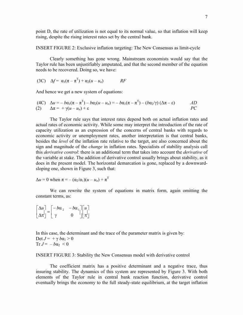
point D, the rate of utilization is not equal to its normal value, so that inflation will keep rising, despite the rising interest rates set by the central bank.

INSERT FIGURE 2: Exclusive inflation targeting: The New Consensus as limit-cycle

Clearly something has gone wrong. Mainstream economists would say that the Taylor rule has been unjustifiably amputated, and that the second member of the equation needs to be recovered. Doing so, we have:

(3C) Δf = α1(π – πT) + α2(u – un) RF

And hence we get a new system of equations:

(4C) Δu = – bα1(π – πT) – bα2(u – un) = – bα1(π – πT) – (bα2/γ) (Δπ – ε) AD(2) Δπ = + γ(u – un) + ε PC

The Taylor rule says that interest rates depend both on actual inflation rates and actual rates of economic activity. While some may interpret the introduction of the rate of capacity utilization as an expression of the concerns of central banks with regards to economic activity or unemployment rates, another interpretation is that central banks, besides the level of the inflation rate relative to the target, are also concerned about the sign and magnitude of the change in inflation rates. Specialists of stability analysis call this derivative control: there is an additional term that takes into account the derivative of the variable at stake. The addition of derivative control usually brings about stability, as it does in the present model. The horizontal demarcation is gone, replaced by a downward-sloping one, shown in Figure 3, such that:

Δu = 0 when π = – (α2/α1)(u – un) + πT

We can rewrite the system of equations in matrix form, again omitting the constant terms, as:

ubbu

012

In this case, the determinant and the trace of the parameter matrix is given by:Det J = + γ bα1 > 0Tr J = – bα2 < 0

INSERT FIGURE 3: Stability the New Consensus model with derivative control

The coefficient matrix has a positive determinant and a negative trace, thus insuring stability. The dynamics of this system are represented by Figure 3. With both elements of the Taylor rule in central bank reaction function, derivative control eventually brings the economy to the full steady-state equilibrium, at the target inflation

8

rate. As in the previous figure, inflation rates rise whenever the actual utilization rate exceed the normal utilization rate (whenever the economy is on the right-hand side of the vertical demarcation line), and they drop in the opposite case. The other demarcation line, the downward-sloping one, tells us when central banks will not modify the interest rate, and hence, all else equal, when the rate of utilization will remain unchanged. When, for a given rate of utilization, the economy is above this demarcation line, thus at a higher inflation rate, the central bank will raise interest rates and hence the rate of utilization will tend to fall. And obviously, when the economy is at a lower inflation rate, below the demarcation line, the central bank will lower interest rates and hence rates of utilization will tend to increase. As shown by the arrowheads and the phase trajectory, thanks to derivative control, the economy will eventually reach its equilibrium (π = πT and u = un), which is now a stable focus. In a sense the trajectory followed by such an economy is not that different from the one described in Figure 1. The points A, B, C and D of Figure 3 are the approximate equivalents of the same points in Figure 1.

4. First post-Keynesian amendment : A horizontal Phillips curve segment2

The first three diagrams assumed that there was a unique NAIRU, corresponding to what we called the normal rate of capacity utilization, which some authors, such as Emery and Chang (1997) or McElhattan (1978), also call the NAICU (the non-accelerating inflation capacity utilization) or the SICUR (the stable inflation capacity utilization rate). But what if there is a multiplicity of NAICU? What if there is a whole range of rates of capacity utilization such that the inflation rate remains constant? In other words, what if the NAICU is a wide band rather than a thin line?

There is now a substantial amount of empirical evidence that this is indeed the case. Several authors are now claiming that the Phillips curve has a middle segment which is flat (Eisner, 1996; Filardo, 1998; Barnes and Olivei, 2003; Kim, 2007). In other words, for rates of unemployment or for rates of capacity utilization that are neither too large nor too low, the rate of inflation tends to remain where it is, unless subjected to supply-side shocks. How can that be?

Two reasons have been advanced. The first reason, which central bankers enjoy suggesting, is based on the credibility of the monetary authorities. With inflation targeting, the inflation target becomes a benchmark, which economic agents take into account when making wage and price decisions. As a result, as long as the fluctuations in the real economy are not too large, the inflation target of the central bank will act as an attractor. The second reason, mostly suggested by post-Keynesian authors, is linked to inertia and the shape of the cost curves of firms. According to post-Keynesians, marginal cost curves in most industries are essentially flat, or even slightly downward-sloping, up to full capacity (Lavoie 1992, ch. 3). But most firms operate below capacity. An increase in rates of capacity utilization does not generate upward price pressures of upward inflation pressures, as it does within the standard neoclassical model with upward-sloping marginal cost curves and demand-led inflation. Within this post-Keynesian model of the firm, inertia will keep wage and price inflation where they are, within a fairly large range of rates of utilization (Hein, 2002; Kim, 2007). Thus, within this range, changes in real

2 This section draws implications from a critique of the New Consensus that can be found in Kriesler and Lavoie (2007).

9

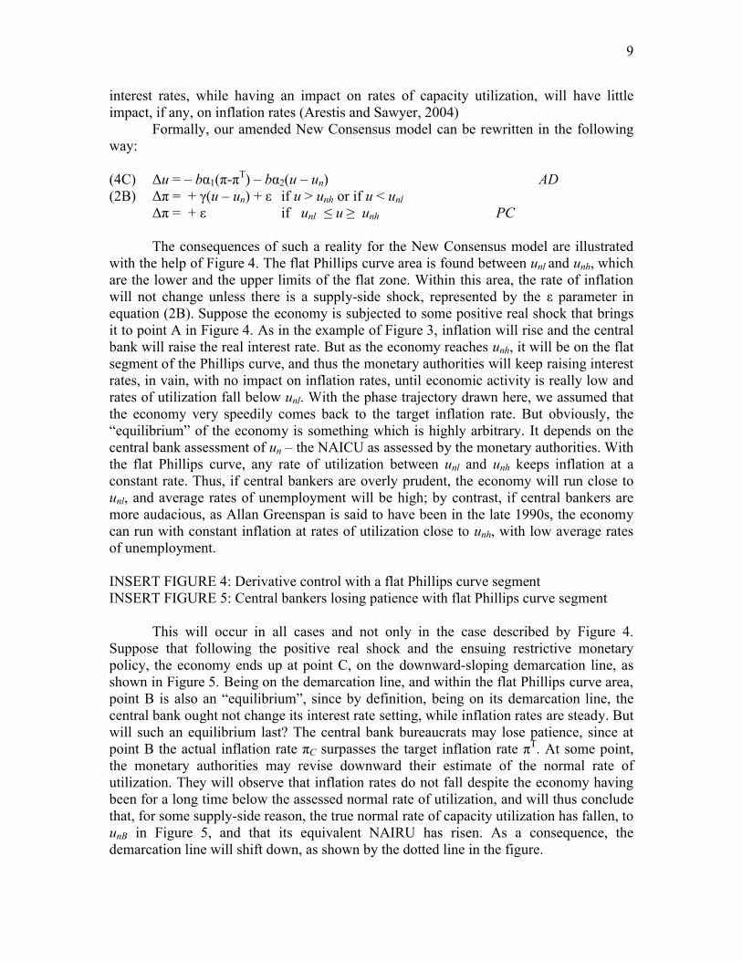
interest rates, while having an impact on rates of capacity utilization, will have little impact, if any, on inflation rates (Arestis and Sawyer, 2004)

Formally, our amended New Consensus model can be rewritten in the following way:

(4C) Δu = – bα1(π-πT) – bα2(u – un) AD(2B) Δπ = + γ(u – un) + ε if u > unh or if u < unl

Δπ = + ε if unl ≤ u ≥ unh PC

The consequences of such a reality for the New Consensus model are illustrated with the help of Figure 4. The flat Phillips curve area is found between unl and unh, which are the lower and the upper limits of the flat zone. Within this area, the rate of inflation will not change unless there is a supply-side shock, represented by the ε parameter in equation (2B). Suppose the economy is subjected to some positive real shock that brings it to point A in Figure 4. As in the example of Figure 3, inflation will rise and the central bank will raise the real interest rate. But as the economy reaches unh, it will be on the flat segment of the Phillips curve, and thus the monetary authorities will keep raising interest rates, in vain, with no impact on inflation rates, until economic activity is really low and rates of utilization fall below unl. With the phase trajectory drawn here, we assumed that the economy very speedily comes back to the target inflation rate. But obviously, the “equilibrium” of the economy is something which is highly arbitrary. It depends on the central bank assessment of un – the NAICU as assessed by the monetary authorities. With the flat Phillips curve, any rate of utilization between unl and unh keeps inflation at a constant rate. Thus, if central bankers are overly prudent, the economy will run close to unl, and average rates of unemployment will be high; by contrast, if central bankers are more audacious, as Allan Greenspan is said to have been in the late 1990s, the economy can run with constant inflation at rates of utilization close to unh, with low average rates of unemployment.

INSERT FIGURE 4: Derivative control with a flat Phillips curve segmentINSERT FIGURE 5: Central bankers losing patience with flat Phillips curve segment

This will occur in all cases and not only in the case described by Figure 4. Suppose that following the positive real shock and the ensuing restrictive monetary policy, the economy ends up at point C, on the downward-sloping demarcation line, as shown in Figure 5. Being on the demarcation line, and within the flat Phillips curve area, point B is also an “equilibrium”, since by definition, being on its demarcation line, the central bank ought not change its interest rate setting, while inflation rates are steady. But will such an equilibrium last? The central bank bureaucrats may lose patience, since at point B the actual inflation rate πC surpasses the target inflation rate πT. At some point, the monetary authorities may revise downward their estimate of the normal rate of utilization. They will observe that inflation rates do not fall despite the economy having been for a long time below the assessed normal rate of utilization, and will thus conclude that, for some supply-side reason, the true normal rate of capacity utilization has fallen, to unB in Figure 5, and that its equivalent NAIRU has risen. As a consequence, the demarcation line will shift down, as shown by the dotted line in the figure.

10

No doubt, a symmetric kind of reasoning could occur if the economy were to wind up at point D, with high rates of capacity utilization and a steady lower-than-the-target inflation rate. Central bankers could modify upwards their estimate of the normal rate of capacity utilization, and the demarcation line would shift up accordingly. Another possibility, however, and one that seems to be tempting to central bankers lately, is to reconsider the inflation target. Some central banks, such as the Bank of Canada, that have been successful at keeping inflation around its target rate are considering the adoption of lower inflation targets. In this case, the demarcation line would shift down, and the central bank would raise interest rates, thus reducing economic activity.

What is interesting here is that, depending on where the transition dynamics bring the economy, several different configurations are possible. In other words, such an economy with a flat Phillips curve segment is path-dependent. There is not a unique equilibrium, as the standard New Consensus model. There is a multiplicity of possible equilibria, that depend on the transition dynamics and the estimates of the central bank.

5. Second post-Keynesian amendment: Unemployment hysteresis3

So far capital accumulation has been omitted. Estimates of Phillips curves were initially based on unemployment rates, but many estimates are based on rates of capacity utilization, as in the previous sections, but also on growth rates of real output (Goodhart, 2003). One reason for this is unemployment hysteresis, an hypothesis put forward by both New Keynesian and post-Keynesian economists, and for which there is considerable empirical evidence (McDonald, 1995; Stanley, 2004). Within the context of the traditional Phillips curve, hysteresis implies that changes in wage and price inflation depend essentially on the change in the unemployment rate, rather than its level, a claim that, surprisingly, could already be found more than forty years ago in Bowen and Berry (1963). The main justification for this is that employed workers have little reason to fear the possibility of losing their job as long as the rate of unemployment is not rising. But the faster unemployment is rising the more threatened workers feel, and the more likely they are to waive real wage objectives. Formally, this implies that we have:

(2C) Δπ = γ(ΔU) + ε PC

Where U is the rate of unemployment.But what is the relationship with growth rates? In a model where labour

employment is roughly proportional to real output, the growth rate of employment, noted e, is given by:

(6) e = g – λ

where g is the growth rate of real output, while λ is the growth rate of technical progress as measured by labour productivity.

3 This section is mainly inspired by Lavoie (2006), which was first presented at the University of Burgundy in 2002. See also Lavoie (1992, pp. 405-7).

11

A traditional concept in economics is the concept of the natural rate of growth, which we denote by gn. This natural rate of growth is the sum of the growth rate of the labour force, which we denote by n, and the growth rate of technical progress, so that:

(7) gn = n + λ

Putting equations (6) and (7) together, and remembering that the change in the rate of unemployment is approximately equal to the difference between the rate of growth of the labour force and that of employment, we get:

(8) ΔU = n – e = gn – g

The change in the rate of unemployment is thus also equal to the difference between the natural and the actual rate of growth of the economy. On that basis, we can rewrite the entire simple New Consensus model of section 2, in terms of growth rates, in a way which is very much analogous. We have:

(1D) g = a – bf IS(2D) Δπ = γ(g – gn) + ε PC(3D) f = f0 + α1(π – πT) RF

In equations (1D), (2D) and (3D), the actual and natural growth rates g and gn

play exactly the same role as u and un were playing in the initial basic model given by equations (1), (2) and (3).4 The actual output growth is said to depend negatively on real interest rates; changes in inflation are caused by changes in the rate of unemployment; and real interest rates are set on the basis of the difference between actual and target inflation. The graphical representation of our new model is thus exactly similar to that of Figure 1. We get the same results. Following any temporary or permanent shock, the growth rate of real output will be brought back to the natural rate of growth. If the monetary authorities assess correctly the natural rate of interest, the target inflation rate will be achieved. Thus, in analogy with the model of Figure 1, the actions being pursued by the monetary authorities have no impact on the natural rate of growth, they only have an impact on the inflation rate.

However, there is one difference. In the model of Figure 1, the choice of a lower inflation target would have had no effect on the rate of utilization and the rate of unemployment. Here, by contrast, there is unemployment hysteresis. The choice of a lower inflation target would force the appearance of a sequence of periods during which the actual growth rate of real output, g, is smaller than the natural rate of growth of theeconomy, gn, as would occur in Figure 1 when the economy moves to point D and then from D to A. As a result, as can be read off equation (7), the rate of unemployment would be rising during a number of periods. Once the economy is back to point A, where the

4 To introduce capital accumulation, an alternative to the suggested amended model would be to keep equations (1), (2), and (3) as they are, while adding the following equation :g = gn + µ (u un)in which case the efforts of the central bank to bring back the economy to its its normal level of capacity utilization would also bring back the actual growth rate to its natural level.

12

target inflation rate is achieved with g = gn, the rate of unemployment U is constant, but it is higher than it was before the decision to have a lower inflation target. Thus, within this framework, there is also no unique NAIRU, although long-run growth is supply-led, being determined by the natural rate of growth (Taylor, 2000, p. 91).

6. Third post-Keynesian amendment: Unemployment and growth hysteresis5

Post-Keynesians however make a further argument. They believe that if the concept of a natural growth rate is to be of any assistance, it is determined by the path taken by the actual growth rate. The most likely candidate for endogenous changes in the natural rate of growth induced by high growth rates of demand is the rate of technical progress. This argument was made by Joan Robinson in her magnum opus.

But at the same time technical progress is being speeded up to keep up with accumulation. The rate of technical progress is not a natural phenomenon that falls like the gentle rain from heaven. When there is an economic motive for raising output per man the entrepreneurs seek out inventions and improvements. Even more important than speeding up discoveries is the speeding up of the rate at which innovations are diffused. When entrepreneurs find themselves in a situation where potential markets are expanding but labour hard to find, they have every motive to increase productivity (Robinson 1956, p. 96).

And it was also a point made by Nicholas Kaldor in a lecture in 1954:

The stronger the urge to expand … the greater are the stresses and strains to which the economy becomes exposed; and the greater are the incentives to overcome physical limitations on production by the introduction of new techniques. Technical progress is therefore likely to be greatest in those societies where the desired rate of expansion of productive capacity … tends to exceed most the expansion of the labour force (which, as we have seen, is itself stimulated, though only up to certain limits, by the growth in production) (Kaldor, 1960, p. 237).

Formally, there might be an increase in the rate of growth of productivity as long as the natural rate of growth does not catch up with the actual rate of accumulation (the rate of productivity growth will decline as long as the natural rate of growth exceeds the actual rate), which we can write as:

(7) ∆gn = φ(g – gn)

5 This section is mainly inspired by Lavoie (2006), where more details and graphs can be found. See also Dutt (2006) for a similar approach, and also Cornwall (1977).

13

Thus, in the world described by equations (1D), (2D) , (3D) and (7), the decision to reduce the target inflation rate is likely to bring about not only a higher rate of unemployment but also a permanently lower growth rate of the economy. Putting these four equations together yields a system of two differential equations. This can be shown by rewriting equation (1D) in difference form. We get:

(1E) Δg = – bΔf

Similarly, by rewriting equation (3E) in difference form, we have:

(3D) Δf = α1Δπ

So that putting together these two equations, we have:

(4E) Δg = – bα1Δπ

Bringing back equation (2D), we finally get:

(4F) Δg = – bα1γ(g – gn) + ε

The system of differential equations is made up of equations (4F) and (7). In matrix form, omitting again the constant terms, we have:

nn g

gbb

g

g 11

with:Det J = 0Tr J = – (bα1γ + φ) < 0

The determinant of the coefficient matrix is equal to zero. We have a zero-rootdynamic system. This implies that there is a single demarcation line, where both ∆gn = 0 and Δg = 0, with a continuum of potential equilibria on that line. These equilibria are stable, because the trace of the coefficient matrix is negative. Thus as shown in Figure 6, if the central bank raises real interest rates and reduces the growth rate of real output in an effort to achieve a lower inflation target, bringing the economy to point D, in both Figures 1 and 6, the economy will not come back to its initial growth rate gn when it finally achieves its target inflation rate; instead the economy will settle at a some lower growth rate, shown in Figure 6 for instance as gnD. Symmetrically, a positive shock on aggregate demand that would momentarily raise the growth rate of the economy to gB

would also end up raising the natural rate of growth to a level such as gnB. Once again we have a case of hysteresis, in both unemployment and growth. There is path dependence, as the initial state and the transition dynamics, through the values of the reaction parameters γ and φ have an impact on the final equilibrium. Hence there is an infinite number of possible equilibria, all with a different constant unemployment rate and a different growth rate.

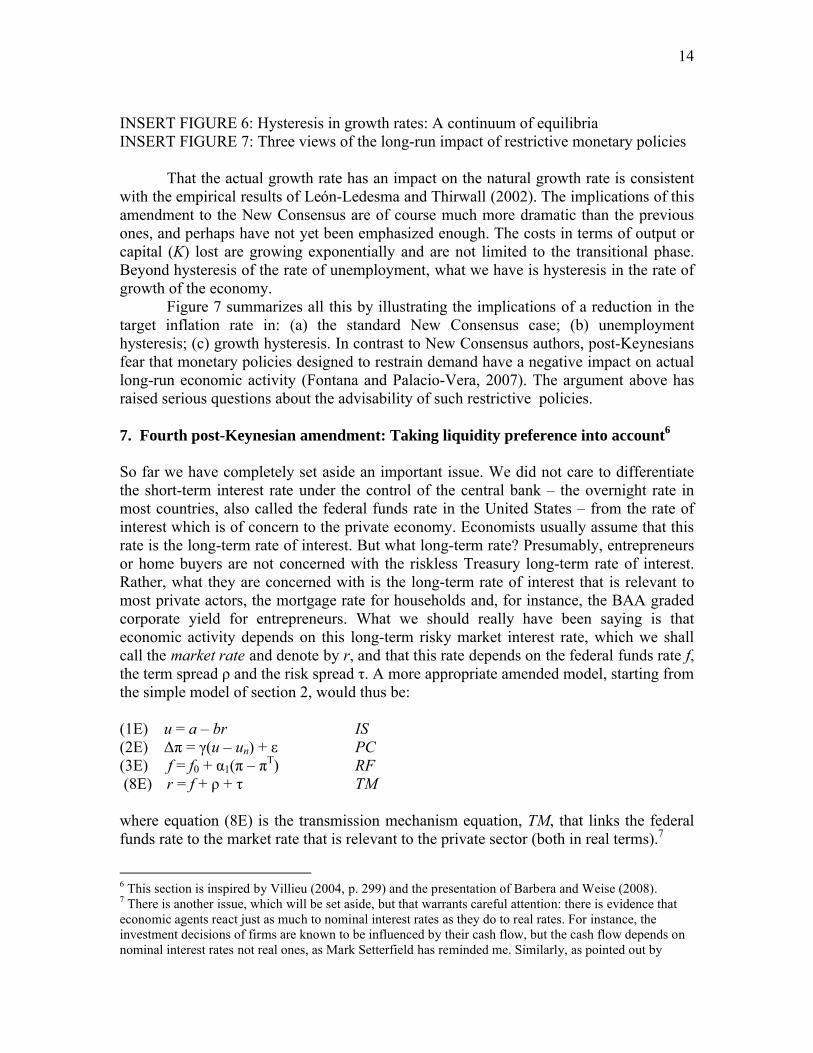
14

INSERT FIGURE 6: Hysteresis in growth rates: A continuum of equilibriaINSERT FIGURE 7: Three views of the long-run impact of restrictive monetary policies

That the actual growth rate has an impact on the natural growth rate is consistent with the empirical results of León-Ledesma and Thirwall (2002). The implications of this amendment to the New Consensus are of course much more dramatic than the previous ones, and perhaps have not yet been emphasized enough. The costs in terms of output or capital (K) lost are growing exponentially and are not limited to the transitional phase. Beyond hysteresis of the rate of unemployment, what we have is hysteresis in the rate of growth of the economy.

Figure 7 summarizes all this by illustrating the implications of a reduction in the target inflation rate in: (a) the standard New Consensus case; (b) unemployment hysteresis; (c) growth hysteresis. In contrast to New Consensus authors, post-Keynesians fear that monetary policies designed to restrain demand have a negative impact on actual long-run economic activity (Fontana and Palacio-Vera, 2007). The argument above has raised serious questions about the advisability of such restrictive policies.

7. Fourth post-Keynesian amendment: Taking liquidity preference into account6

So far we have completely set aside an important issue. We did not care to differentiate the short-term interest rate under the control of the central bank – the overnight rate in most countries, also called the federal funds rate in the United States – from the rate of interest which is of concern to the private economy. Economists usually assume that this rate is the long-term rate of interest. But what long-term rate? Presumably, entrepreneurs or home buyers are not concerned with the riskless Treasury long-term rate of interest. Rather, what they are concerned with is the long-term rate of interest that is relevant to most private actors, the mortgage rate for households and, for instance, the BAA graded corporate yield for entrepreneurs. What we should really have been saying is that economic activity depends on this long-term risky market interest rate, which we shall call the market rate and denote by r, and that this rate depends on the federal funds rate f, the term spread ρ and the risk spread τ. A more appropriate amended model, starting from the simple model of section 2, would thus be:

(1E) u = a – br IS(2E) Δπ = γ(u – un) + ε PC(3E) f = f0 + α1(π – πT) RF(8E) r = f + ρ + τ TM

where equation (8E) is the transmission mechanism equation, TM, that links the federal funds rate to the market rate that is relevant to the private sector (both in real terms).7

6 This section is inspired by Villieu (2004, p. 299) and the presentation of Barbera and Weise (2008).7 There is another issue, which will be set aside, but that warrants careful attention: there is evidence that economic agents react just as much to nominal interest rates as they do to real rates. For instance, the investment decisions of firms are known to be influenced by their cash flow, but the cash flow depends on nominal interest rates not real ones, as Mark Setterfield has reminded me. Similarly, as pointed out by

15

Figure 1 needs to be a bit more complicated now. We need to dispatch the 45-degree quadrant, and introduce the transmission mechanism equation. The reaction function equation is moved to the south-west quadrant, while the transmission mechanism equation makes its appearance in the fourth quadrant – the north-west quadrant – as drawn in Figure 8.

What difference does this make? It helps to understand and picture was has been occurring on financial markets since August 2007. Several observers of the financial scene have described the recent financial turmoil as a ‘Minsky moment’. Hyman Minsky (1986) is a post-Keynesian economist who paid considerable attention to financial markets, debt ratios, stock-flow relations, and liquidity preference. In particular, he argued that capitalism inherently brings about fragile financial structures, as bankers and borrowers forget about past crises, taking ever risky positions that eventually generate defaults, insolvencies, and falling asset prices, as seems to be the case since 2007. In a nutshell, his view, as argued by Joan Robinson, was that tranquillity breeds instability. Had he known about the New Consensus, Minsky would have been most certainly quite appalled by its simple 3-equation apparatus that ignores payment flows arising from debt stocks as well as fluctuations in asset prices.

INSERT FIGURE 8: The four-quadrant New Consensus model upgraded with liquidity preference

But how can some of Minsky’s concerns be dealt with within the model of Figure 8? In a ‘Minsky moment’, the risk spread τ rises considerably.8 As there is a rush towards liquidity and riskless assets, the prices of risky assets fall, and hence the interest rates on these assets rise. In figure 8, this can be represented by an upward shift of the TM curve, from TM1 to TM2. Thus, even if the financial crisis does not have a direct impact on the real economy – meaning here that the a coefficient in the IS equation remains put, there will be consequences for the real economy because market rates will rise from r1 to r2. If the central bank does not modify its reaction function, the aggregate demand curve AD will get shifted downwards and economic activity will fall to u2, with the economy moving from point A to point B. Then, as the inflation rates start to fall, as a result of the rates of capacity utilization being below their normal levels, nominal and real federal funds rate will be brought down by the central bank, moving along the RF1 reaction function. If the monetary authorities react in the normal way, without taking into account the turmoil in the financial markets and the higher risk premia, the economy will be brought back to the normal rate of capacity utilization, but at a steady rate of inflation that will be below the target, at point C. In other words, the risk premium in financial markets acts like a negative shock on the aggregate demand curve, just like a real negative shock would. If this financial shock is large enough it could even bring about negative inflation, and hence debt-deflation as argued by Minsky.

Haight (2007-8), mortgage loans to households are usually granted on the basis of various measures of cash flow expenditures on housing relative to current income, and thus are based on nominal interest rates and not real rates (unless expected future housing price increases are taken into account, a cause of the subprime crisis). Doing justice to this issue would require more than an amendment to the New Consensus model. 8 The term premium could also be considered, but we won’t do it here.

16

The higher risk premium requires the central bank to modify its assessment of the natural rate of interest, f0, in a counter-intuitive way, since it must reduce the federal funds rate when long-term market interest rates are rising. The monetary authorities must shift their reaction function, to RF3, and reduce the federal funds rate at f3 in order to keep inflation on target at πT and avoid a reduction in economic activity (thus keeping market interest rates at r1). The central bank cannot claim, as it sometimes does, that long-term market rates are a proper proxy for the natural interest rate and a guide to help setting the federal funds rate. In the present case, if the central bank were raise its estimate of the natural rate of interest, in an effort to follow the apparent increase in long-term market rates, it would only make matters worse.

7. Conclusion

New Consensus authors are certainly on the right track when they model interest rate targeting – a requirement of macro models long made by post-Keynesian authors. But as pointed out by Pollin (2003, p. 293), their hypothesis of a unique stable equilibrium is unwarranted and leads to overly simplistic policy prescriptions. I hope to have shown that it was relatively easy to introduce hysteresis effects by amending the New Consensus model. The introduction of liquidity preference effects also enriches the model, showing that the life of central bankers in setting interest rates is far from being simple, even if they only assign to themselves the task of keeping inflation rates stable. Whether this ought to be their main task is another issue, discussed by others.9

References

P. Arestis and M. Sawyer, ‘Can Monetary Policy Affect the Real Economy?’, European Review of Economics and Finance, 3 (2), (2004) 9-32.

M.L. Barnes. and G.P. Olivei, ‘Inside and Outside Bounds: Estimates of the Phillips Curve’. New England Economic Review , (2003) 3-18.

R.J. Barbera and C.L. Weise, ‘A Minsky/Wicksell Modified Taylor Rule’, presentation made at the 17th Minsky Conference, Levy Economics Institute of Bard College, 18 April 2008.

U. Bindseil, Monetary Policy Implementation: Theory, Past and Present (Oxford; Oxford University Press, 2004).

W. G. Bowen and R.A. Berry, ‘Unemployment and Movements of the Money Wage Level’, Review of Economics and Statistics, 45 (2), May (1963) 163-172.

J. Cornwall, Modern Capitalism: its Growth and Transformation (London: Martin Roberstson, 1977).

A.B. Cramp, ‘Monetary Policy: Strong or Weak’, in N. Kaldor (ed.), Conflict in Policy Objectives (Oxford: Basil Blackwell, 1971), pp. 62-74.

9 See in particular the special issue of the Journal of Post Keynesian Economics, edited by Rochon (2007).

17

A.K. Dutt, ‘Aggregate Demand, Aggregate Supply and Economic Growth’, International Review of Applied Economics, 20 (3), July (2006) 319-336.

R. Eisner, ‘The Retreat from Full Employment’, in P. Arestis (ed.), Employment, Economic Growth and the Tyranny of the Market: Essays in Honour of Paul Davidson, Volume Two (Cheltenham: Edward Elgar, 1996), pp. 106-130.

K.M. Emery and C.P. Chang, ‘Is There a Stable Relationship Between Capacity Utilization and Inflation?’. Federal Reserve Bank of Dallas Economic Review, 1 (1997) 14-20.

A.J. Filardo, ‘New Evidence on the Output Cost of Fighting Inflation’, Federal Reserve Bank of Kansas City Quarterly Review, 83 (3), (1998) 33-61.

G. Fontana and A. Palacio-Vera, ‘Are Long-run Price Stability and Short-run Output Stabilization all that Monetary Policy Can Aim for?’, Metroeconomica, 57 (2), (2007) 269-298.

D. Fuller and D. Geide-Stevenson, ‘Consensus among economists: revisited’, Journal of Economic Education 34 (4), (2003) 369-87.

S.T. Fullwiler, ‘Timeliness and the Fed’s Daily Tactics’, Journal of Economic Issues, 37 (4), (2003) 851-880.

C. Goodhart, ‘What is the Monetary Policy Committee Attempting to Achieve?’, in Macroeconomics, Monetary Policy and Financial Stability: A Festschrift in Honour of Charles Freedman (Ottawa: Bank of Canada, 2003), pp. 153-169.

A.D. Haight, ‘A Keynesian Angle for the Taylor Rule: Mortgage Rates, Monthly Payment Illusion, and the Scarecrow Effect of Inflation’, Journal of Post Keynesian Economics, 30 (2), Winter (2007-8) 259-278.

E. Hein, ‘Monetary Policy and Wage Bargaining in the EMU: Restrictive ECB Policies, High Unemployment, Nominal Wage Restraint and Inflation Above the Target’, Banca del Lavoro Quarterly Review, 222, September (2002) 299-337.

T.M. Humphrey, ‘Fisherian and Wicksellian Price-stabilization Models in the History of Monetary Thought’, Federal Reserve Bank of Richmond Economic Review, 76 (3), May-June (1990) 3-12.

N. Kaldor, ‘Characteristics of Economic Development’, in Essays on Economic Stability and Growth (London: Duckworth, 1960), pp. 232-242.

J.H. Kim, Three Essays on Effective Demand, Economic Growth and Inflation, PhD. Dissertation, Department of Economics, University of Ottawa (2007).

P. Kriesler and M. Lavoie (2007), ‘The New View on Monetary Policy: The New Consensus and its Post-Keynesian Critique’, Review of Political Economy, 19 (3), July (2007) 387-404.

M. Lavoie, Foundations of Post-Keynesian Economic Analysis (Aldershot: Edward Elgar, 1992).

M. Lavoie, ‘A Post-Keynesian Amendment to the New Consensus on Monetary Policy’, Metroeconomica, 57 (2), (2006) 165-192.

18

M.A. León-Ledesma and A.P. Thirlwall, ‘The Endogeneity of the Natural Rate of Growth’, Cambridge Journal of Economics, 26 (4), July (2002) 441-459.

L.M. McDonald, ‘Models of the Range of Equilibria’, in R. Cross (ed.), The Natural Rate of Unemployment: Reflections on 25 Years of the Hypothesis, (Cambridge: Cambridge University Press, 1995), pp. 101-152.

R. McElhattan, ‘Estimating a Stable-Inflation Capacity-Utilization Rate’, Federal reserve Bank of San Franciso Economic Review, 78, Fall (1978) 20-30.

H.P. Minsky, Stabilizing an Unstable Economy (New Haven: Yale University Press, 1986). Reprinted in 2008 (New York: McGraw-Hill).

A. Orphanides and J.C. Williams, ‘Robust Monetary Rules with Unknown Natural Rates’, Brookings Papers on Economic Activity, 2, (2002) 63-145.

J.P. Pollin, ‘Une Macroéconomie sans LM: Quelques Propositions Complémentaires’,Revue d’ Economie Politique, 113 (3), (2003) 273-293.

W. Poole (1970), ‘Optimal Choice of Monetary Policy Instruments in a Simple Stochastic Macro Model’, Quarterly Journal of Economics, 84 (1970) 197-216.

J. Robinson, The Accumulation of Capital (London: Macmillan, 1956).

L.P. Rochon, ‘The State of Post Keynesian Interest Rate Policy: Where are We and Where are We Going?’, Journal of Post Keynesian Economics, 30 (1), Fall (2007) 3-12.

M. Setterfield, ‘Central Bank Behaviour and the Stability of Macroeconomic Equilibrium: A Critical Examination of the “New Consensus”’, in P. Arestis, M. Baddeley and J.S.L. McCombie (eds), The New Monetary Policy: Implications and Relevance, (Cheltenham: Edward Elgar, 2005), pp. 23-49.

T.D. Stanley, ‘Does Unemployment Hysteresis Falsify the Natural Rate Hypothesis? A meta-regession analysis’, Journal of Economic Surveys, 18 (4), (2004) 589-612.

J.B. Taylor, ‘Teaching Modern Macroeconomics at the Principles Level’, American Economic Review, 90 (2), May (2000) 90-94.

P. Villieu, ‘Une Macroéconomie sans LM: Un Modèle de Synthèse pour l’Analyse des Politiques Conjoncturelles’, Revue d’ Economie Politique, 114 (3), (2004) 289-322.

19

Slide 1 Figure 1

IS1

AD2

f3f

u

u

RF1

MP

un

IA

u1

T

2

f1

f2

AB

C

A

BC

u3

D

D

AD1

IS2

RF2

Slide 2Figure 2

Δπ

unhunl

u

Slide 3 Figure 3

IS1

AD2

f3f

u

u

RF1

unu1

T

2

f1

f2

A

BC

AC

u3

D

D

AD1

RF2

unhunl

f4

E

E

20

Slide 4 Figure 4

IS

AD1

rr

g

RF3

gnB gnC

C

E

rB

rC

C

EB

E

B*

gnE

B

rE

T

gB

C

rB*

B*

RF2

g

AD2AD3

B’

E’

Slide 5Figure 5

g

gn45° line

gnE

gnE

gnCgnBgB

B’

B

B*

E

C

Slide 6Figure 6a

Time

Log KSlope isgn = n + λ

Actual path

21

Slide 7Figure 6b

Time

Log KSlopes are gn = n + λ

Actual path

Slide 8Figure 6c

Time

Log K Slope isgn = n + λ

New slope

Actual path

Slide 9 Figure 7

AD2

r

u

u

f

f

RF1

un

IA

T

2

r1

r2

C

A

A

u2

B

B

AD1

IS

RF2

TM1

TM2 r

f1f2

A

AA’

A’