Impact of TraÆc Aggregation on Network Capacity

and Quality of Service

by

Towela P.R. Nyirenda-Jere

B.Sc (EE), University of Malawi, 1992

M.Sc (EE), University of Kansas, 1996

Submitted to the Department of Electrical Engineering and Computer

Science and the Faculty of the Graduate School of the University of Kansas

in partial ful�llment of the requirements for the degree of Doctor of Philos-

ophy.

Contents

1 Introduction and Motivation 1

2 TraÆc Aggregation, Quality of Service and Network Capac-

ity 6

3 Background 11

3.1 Quality of Service . . . . . . . . . . . . . . . . . . . . . . . . . 11

3.2 Scheduling Mechanisms . . . . . . . . . . . . . . . . . . . . . . 14

3.3 Network Design . . . . . . . . . . . . . . . . . . . . . . . . . . 22

4 Network Analysis using Network Calculus 27

4.1 Principles of Network Calculus . . . . . . . . . . . . . . . . . . 27

4.2 End-to-End Delay Analysis . . . . . . . . . . . . . . . . . . . 35

5 Analytic Framework 39

i

5.1 Notation . . . . . . . . . . . . . . . . . . . . . . . . . . . . . . 39

5.2 Application Characterization . . . . . . . . . . . . . . . . . . . 40

5.3 TraÆc Handling Mechanisms . . . . . . . . . . . . . . . . . . . 42

6 TraÆc Aggregation in a Single Network Node 44

6.1 Analysis and Methodology . . . . . . . . . . . . . . . . . . . . 44

6.2 Numerical Results for Single Network Node . . . . . . . . . . 46

6.2.1 Capacity Requirements with Varying Voice Load . . . 46

6.2.2 Capacity Requirements with Varying WWW Load . . . 50

6.2.3 Delay Performance with changes in load . . . . . . . . 52

6.2.4 Required Capacity with Projections on TraÆc Growth 55

6.2.5 Capacity Requirements with Varying Delay Guarantees 57

6.2.6 Capacity Requirements with Varying Burstiness . . . . 59

6.3 Summary . . . . . . . . . . . . . . . . . . . . . . . . . . . . . 60

7 Network Analysis 61

7.1 General Network Topology . . . . . . . . . . . . . . . . . . . . 61

7.2 Analysis of Network Capacity Requirements . . . . . . . . . . 63

7.3 Preliminary Equations and Parameters . . . . . . . . . . . . . 64

7.4 Edge Capacity Requirements . . . . . . . . . . . . . . . . . . . 65

ii

7.5 Core Capacity Requirements . . . . . . . . . . . . . . . . . . . 66

7.6 Numerical Results for Network Analysis . . . . . . . . . . . . 69

7.6.1 Topology Construction . . . . . . . . . . . . . . . . . . 69

7.6.2 Parameters . . . . . . . . . . . . . . . . . . . . . . . . 70

7.6.3 Capacity Requirements with Symmetric TraÆc Distri-

bution . . . . . . . . . . . . . . . . . . . . . . . . . . . 71

7.6.4 E�ect of Projections on TraÆc Growth . . . . . . . . . 79

7.6.5 Impact of Burstiness on Edge and Core Capacity . . . 80

7.6.6 E�ect of Delay Ratios . . . . . . . . . . . . . . . . . . 81

7.7 Summary . . . . . . . . . . . . . . . . . . . . . . . . . . . . . 83

8 Bounds on Capacity Requirements 85

8.1 Single-Link . . . . . . . . . . . . . . . . . . . . . . . . . . . . 85

8.2 Edge-Core Network . . . . . . . . . . . . . . . . . . . . . . . . 87

8.2.1 WFQ Core . . . . . . . . . . . . . . . . . . . . . . . . . 88

8.2.2 CBQ Core . . . . . . . . . . . . . . . . . . . . . . . . . 89

8.2.3 PQ Core . . . . . . . . . . . . . . . . . . . . . . . . . . 90

8.2.4 FIFO Core . . . . . . . . . . . . . . . . . . . . . . . . . 91

8.3 Numerical Results on Capacity Bounds . . . . . . . . . . . . . 92

iii

9 Aggregation, Network Capacity and Utilization 94

10 Sensitivity Analysis of Capacity Requirements 101

10.1 Uncertainty and Sensitivity Analysis . . . . . . . . . . . . . . 102

10.2 Sensitivity Analysis for a Single Link . . . . . . . . . . . . . . 106

10.3 Numerical Results on Sensitivity Analysis . . . . . . . . . . . 111

10.3.1 Case 1: Single Flow, Small Variance in Delay . . . . . 111

10.3.2 Case 2: Multiple Flows, Small Variance in Delay . . . . 113

10.3.3 Case 3: Increased Video and WWW Variance . . . . . 116

10.3.4 Case 4: Increased Email and WWW Variance . . . . . 119

10.4 Summary . . . . . . . . . . . . . . . . . . . . . . . . . . . . . 122

11 Conclusion 123

11.1 Implications of Results on Network Architectures . . . . . . . 123

11.2 Practical Applications of Sensitivity Analysis . . . . . . . . . . 125

11.3 Summary of Contributions . . . . . . . . . . . . . . . . . . . . 127

11.4 Future Work . . . . . . . . . . . . . . . . . . . . . . . . . . . . 128

iv

List of Figures

2.1 Levels of Aggregation . . . . . . . . . . . . . . . . . . . . . . . 7

2.2 Simple TraÆc handling and Network Capacity Trade-o� . . . 9

2.3 TraÆc handling and Network Capacity Trade-o� with varying

Network Load . . . . . . . . . . . . . . . . . . . . . . . . . . . 10

2.4 Comparison of TraÆc Handling Sensitivity . . . . . . . . . . . 10

3.1 QoS trade-o� in Communication Networks . . . . . . . . . . . 22

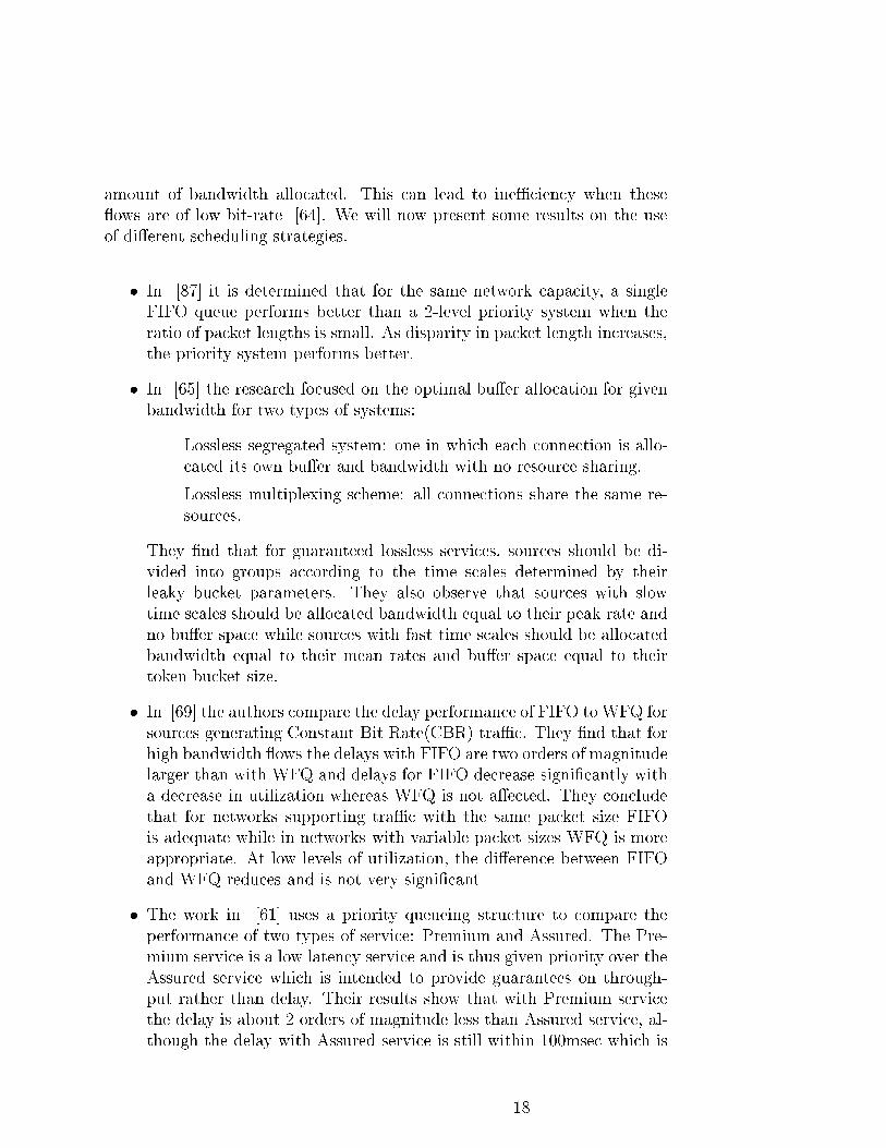
4.1 IETF Arrival Curve . . . . . . . . . . . . . . . . . . . . . . . . 29

4.2 IETF Arrival and Service Curves . . . . . . . . . . . . . . . . 31

4.3 Arrival and Service Curves for FIFO . . . . . . . . . . . . . . 32

4.4 Arrival and Service Curves for PQ . . . . . . . . . . . . . . . . 33

4.5 Arrival and Service Curves for WFQ . . . . . . . . . . . . . . 34

6.1 Capacity Requirement with No Video . . . . . . . . . . . . . . 47

v

6.2 Capacity Requirement with 20% Video . . . . . . . . . . . . . 47

6.3 Capacity Requirement with No Video (� = 0:1) . . . . . . . . 49

6.4 Capacity Requirement with 20% Video (� = 0:1) . . . . . . . 49

6.5 Capacity Requirement with no Video . . . . . . . . . . . . . . 50

6.6 Capacity Requirement with 20% Video . . . . . . . . . . . . . 50

6.7 Capacity Requirement with no Video (� = 0:1) . . . . . . . . 52

6.8 Capacity Requirement with 10% Video(� = 0:1) . . . . . . . 52

6.9 Variation in Voice Delay with increase in Voice load . . . . . . 53

6.10 Variation in WWW Delay with increase in Voice load . . . . . 53

6.11 Variation in Voice Delay with increase in WWW load . . . . . 54

6.12 Variation in WWW Delay with increase in WWW load . . . . 54

6.13 Network Capacity with Projections on Voice and WWW TraÆc 56

6.14 Network Capacity with Projections on Voice and WWW TraÆc 56

6.15 Network Capacity with Projections on Voice and WWW TraÆc 57

6.16 Network Capacity with Projections on Voice and WWW TraÆc 57

6.17 Link Capacity with 10ms bursts . . . . . . . . . . . . . . . . . 59

6.18 Link Capacity with varying burst sizes . . . . . . . . . . . . . 59

7.1 Carrier Topology . . . . . . . . . . . . . . . . . . . . . . . . . 62

vi

7.2 Topology with 5 Core Nodes and 3 links per node . . . . . . . 69

7.3 Edge and Core Capacity with WFQ in the Edge . . . . . . . . 72

7.4 Edge and Core Capacity with WFQ in the Edge . . . . . . . . 72

7.5 Edge and Core Capacity with CBQ in the Edge . . . . . . . . 73

7.6 Edge and Core Capacity with CBQ in the Edge . . . . . . . . 73

7.7 Edge and Core Capacity with PQ in the Edge . . . . . . . . . 74

7.8 Edge and Core Capacity with PQ in the Edge . . . . . . . . . 74

7.9 Edge and Core Capacity with FIFO in the Edge . . . . . . . . 74

7.10 Edge and Core Capacity with FIFO in the Edge . . . . . . . . 74

7.11 Edge and Core Capacity with FIFO in the Edge: 5 nodes

poorly-connected . . . . . . . . . . . . . . . . . . . . . . . . . 78

7.12 Edge and Core Capacity with FIFO in the Edge: 5 nodes

highly-connected . . . . . . . . . . . . . . . . . . . . . . . . . 78

7.13 Edge and Core Capacity with FIFO in the Edge: 20 nodes

poorly-connected . . . . . . . . . . . . . . . . . . . . . . . . . 78

7.14 Edge and Core Capacity with FIFO in the Edge: 20 nodes

highly-connected . . . . . . . . . . . . . . . . . . . . . . . . . 78

7.15 Core Capacity for 20 node network with WFQ in the Edge . . 80

7.16 Core Capacity for 20 node network with FIFO in the Edge . . 80

7.17 Edge Capacity as a function of WWW burstiness . . . . . . . 81

vii

7.18 Core Capacity as a function of WWW burstiness . . . . . . . 81

10.1 WFQ Capacity vs Delay for Video and WWW traÆc for Case

2: small delay variance . . . . . . . . . . . . . . . . . . . . . . 114

10.2 PQ Capacity vs Email Delay for Case 2: small delay variance 115

10.3 WFQ Capacity vs Delay for Video and WWW traÆc for Case

3: increased Video and WWW variance . . . . . . . . . . . . . 118

10.4 WFQ Capacity vs Email and WWW Delay for Case 4: in-

creased Email and WWW variance . . . . . . . . . . . . . . . 120

11.1 Capacity Requirements of Edge and Core TraÆc Handling

Mechanisms . . . . . . . . . . . . . . . . . . . . . . . . . . . . 124

viii

List of Tables

5.1 Network Applications . . . . . . . . . . . . . . . . . . . . . . . 40

5.2 TraÆc Class Parameters . . . . . . . . . . . . . . . . . . . . . 41

5.3 TraÆc Handling Mechanisms . . . . . . . . . . . . . . . . . . . 42

6.1 Maximum Delay for Single-Link Analysis . . . . . . . . . . . . 46

6.2 Capacity as a function of Voice Delay . . . . . . . . . . . . . . 57

6.3 Capacity as a function of WWW Delay . . . . . . . . . . . . . 58

7.1 Maximum End-to-End Delay for Edge-Core Analysis . . . . . 70

7.2 Network Capacity for 20 Node Full-Mesh Network (in equiva-

lent OC3 links) . . . . . . . . . . . . . . . . . . . . . . . . . . 75

7.3 Core Capacity as a function of Network Diameter for WFQ

Edge . . . . . . . . . . . . . . . . . . . . . . . . . . . . . . . . 76

7.4 Core Capacity as a function of Network Diameter for FIFO

Edge . . . . . . . . . . . . . . . . . . . . . . . . . . . . . . . . 76

7.5 Capacity as a function of Voice Delay with WFQ Edge . . . . 81

ix

7.6 Capacity as a function of Voice Delay with FIFO Edge . . . . 82

7.7 Capacity as a function of WWW Delay with WFQ Edge . . . 82

7.8 Capacity as a function of WWW Delay with FIFO Edge . . . 82

8.1 Ratio of CBQ to WFQ Capacity as a function of Voice Delay . 92

8.2 Ratio of PQ to WFQ Capacity as a function of Voice Delay . . 93

8.3 Ratio of FIFO to WFQ Capacity as a function of Voice Delay 93

9.1 Comparison of End-to-End Delay Bounds . . . . . . . . . . . . 99

10.1 Delay Bound Statistics for Case 1: Small Delay Variance . . . 111

10.2 Analytic Results for Case 1: Single Flow per TraÆc Type . . . 112

10.3 WFQ Analytic and Simulation Results for Case 2: Multiple

Flows, small variance . . . . . . . . . . . . . . . . . . . . . . . 113

10.4 CBQ Analytic and Simulation Results for Case 2:Multiple

Flows, small variance . . . . . . . . . . . . . . . . . . . . . . . 114

10.5 PQ Analytic Results for Case 2: Multiple Flows, small variance116

10.6 FIFO Analytic and Simulation Results for Case 2: Multiple

Flows, small variance . . . . . . . . . . . . . . . . . . . . . . . 116

10.7 Delay Bound Statistics for Case 3: increased Video andWWW

variance . . . . . . . . . . . . . . . . . . . . . . . . . . . . . . 117

10.8 WFQ Analytic Results for Case 3: increased Video andWWW

variance . . . . . . . . . . . . . . . . . . . . . . . . . . . . . . 117

x

10.9 CBQ Simulation Results for Case 3: increased Video and

WWW variance . . . . . . . . . . . . . . . . . . . . . . . . . . 118

10.10PQ Simulation Results for Case 3: increased Video andWWW

variance . . . . . . . . . . . . . . . . . . . . . . . . . . . . . . 119

10.11FIFO Simulation Results for Case 3: increased Video and

WWW variance . . . . . . . . . . . . . . . . . . . . . . . . . . 119

10.12Delay Bound Statistics for Case 4: increased Email andWWW

variance . . . . . . . . . . . . . . . . . . . . . . . . . . . . . . 119

10.13WFQ Analytic and Simulation Results for Case 4: increased

Email and WWW variance . . . . . . . . . . . . . . . . . . . . 120

10.14CBQ Simulation Results for Case 4: increased Email and

WWW variance . . . . . . . . . . . . . . . . . . . . . . . . . . 121

10.15PQ Simulation Results for Case 4: increased Email andWWW

variance . . . . . . . . . . . . . . . . . . . . . . . . . . . . . . 121

10.16FIFO Simulation Results for Case 4: increased Email and

WWW variance . . . . . . . . . . . . . . . . . . . . . . . . . . 121

xi

Abstract

The impact of traÆc handling mechanisms on network capacity and support-

ing of Quality of Service (QoS) in the Internet is studied. The emergence of

applications with diverse throughput, loss and delay requirements requires a

network that is capable of supporting di�erent levels of service as opposed to

the single best-e�ort service that was the foundation of the Internet. As a re-

sult the Integrated Services (per- ow) and Di�erentiated Services (Di�serv)

models have been proposed. The per- ow model requires resource reservation

on a per- ow basis while the Di�serv model requires no explicit reservation of

bandwidth for individual ows and instead relies on a set of pre-de�ned ser-

vice types to provide QoS to applications. Flows are grouped into aggregates

having the same QoS requirements and the aggregates are handled by the

network as a single entity with no ow di�erentiation. We refer to this type

of handling as semi-aggregate or class-based. The Best-E�ort model does not

perform any di�erentiation and handles all traÆc as a single aggregate. Each

of these traÆc handling models can be used to meet service guarantees of

di�erent traÆc types, the major di�erence being in the quantity of network

resources that must be provided in each case. The cross-over point at which

the three approaches of aggregate traÆc management, semi-aggregate traÆc

management and per- ow traÆc management become equivalent is found.

Speci�cally, we determine the network capacity required to achieve equiva-

lent levels of performance under these three traÆc management approaches.

We use maximum end-to-end delay as the QoS metric and obtain analytic ex-

pressions for network capacity based on deterministic network analysis. One

key result of this work is that on the basis of capacity requirements, there is

no signi�cant di�erence between semi-aggregate traÆc handling and per- ow

traÆc handling. However Best-E�ort handling requires more capacity that

may be several orders of magnitude greater than per- ow handling.

Chapter 1

Introduction and Motivation

When the Internet �rst came into being it was used primarily as a research

tool and delivered uniform best-e�ort service to all users. The majority of

traÆc carried at this time was primarily data, which did not have very strin-

gent requirements on timely delivery. During the last decade the Internet

has evolved into being more of a commercial entity than a research network

and has experienced tremendous growth in both the volume of traÆc carried

as well as diversity in the type of traÆc carried. The engineering philosophy

behind the Internet was based on the model of a homogenous community

that had common interests rather than on a model of service providers and

customers [49]. The best-e�ort Internet can be considered as consisting of

just one user group in which everyone is allowed to use the network for any

purpose and limits are imposed only when the capacity is not enough to

satisfy demand. It is also assumed that all users behave agreeably during

times of congestion by limiting their usage. The major tool that was used

to engineer the Internet was over-engineering (often referred to as "throwing

bandwidth at the problem") which refers to providing more bandwidth than

the aggregate demand so that every subscriber is given ample access to net-

work resources. The recent growth in network usage both at the commercial

and public level coupled with the advances in high-speed applications how-

ever tends to stretch the limits of over-booking as more and more customers

are demanding and using more bandwidth from the networks while at the

same time having high expectations on the service that they receive.

The emergence of applications with diverse throughput, loss and delay re-

quirements requires a network that is capable of supporting di�erent levels

of service as opposed to the single best-e�ort service that was the foundation

of the Internet. Quality of Service (QoS) has become the buzzword and um-

1

brella term that captures the essence of this shift in paradigm. IP Telephony

is a good example of an application that is driving the push towards QoS on

the Internet and is in fact being touted as today's killer application for the

Internet [44, 77]. Latency rather than bandwidth is the primary issue in pro-

viding voice services in the Internet, thus the traditional approaches of simply

over-engineering may not work as well for this type of application. To pro-

vide a network that caters to these di�erent levels of service requires changes

to network control and traÆc handling functions. Control mechanisms allow

the user and network to agree on service de�nitions, identify users that are

eligible for a particular type of service and let the network allocate resources

appropriately to the di�erent services. TraÆc handling mechanisms are used

to classify and map information packets to the intended service class as well

as controlling the resources consumed by each class. Notable results of the

e�ort to provide Quality of Service in the Internet are the de�nition of Inte-

grated Services and Di�erentiated Services by the Internet Engineering Task

Force (IETF) [7, 8, 9, 21, 45, 46] and Asynchronous Transfer Mode (ATM)

by the ATM Forum [3].

The Integrated Services per- ow model uses resource reservation to provide

delay and throughput guarantees. The per- ow model is based on the idea

that bandwidth must be explicitly managed in order to meet application

requirements therefore resource reservation and admission control are a must

[9, 10]. Advocates of the per- ow model claim that high �delity interactive

audio and video applications need higher quality and more predictable service

than that provided by the best-e�ort Internet and that this can only be

achieved through explicit resource reservation [12].

The Di�erentiated Services model takes a di�erent approach from the per-

ow model in that it does not promote the use of resource reservation. Pro-

ponents of Di�serv argue that a simple priority structure will be suÆcient

to provide Quality of Service in the Internet. One of the arguments against

resource reservation is that in the future bandwidth will be in�nite, therefore

there will be no need for reservations. Advances in �ber-optic communica-

tion may suggest that bandwidth will be so abundant, ubiquitous and cheap

that it will not bene�t network operators to undertake resource reservation

however, one cannot ignore the fact that increases in available bandwidth are

always followed by corresponding development of applications that consume

and exhaust this bandwidth [9, 35]. Trends in the history of communi-

cations indicate that regardless of how much bandwidth is made available,

applications are always created that quickly exhaust the supply.

Another argument against resource reservation models is that simple pri-

ority will be suÆcient to meet the needs of real-time traÆc. This may be

2

true under some conditions but not always. For instance with �xed network

capacity if the number of high priority real-time transmissions increases then

they will all have degraded performance. A third argument against resource

reservation is that it is too expensive because reservation of resources is

wasteful in that not all the reserved resources are used. This is true if all of

the resource is exclusively reserved and thus it must be ensured that there

is a limit on how much guaranteed traÆc is allowed and provisions must be

made for non-real time traÆc to utilize bandwidth unused by real-time traÆc

[35]. Lastly, it has been suggested that delay bounds are not necessary and

throughput bounds are enough. However, guaranteeing minimum through-

put does not automatically result in better delay performance. Delay bounds

must be explicitly guaranteed and enforced.

Opponents of reservation contend that the issue boils down to one of pro-

visioning and that reservation-enabled networks can only provide satisfac-

tory service if the call blocking rate is low. It is believed that by adequate

provisioning, a best-e�ort network can achieve the same performance as a

reservation-based network [12, 34]. As an example consider IP telephony

users who require the network to guarantee to carry their calls with a max-

imum end-to-end latency that is no larger than 100msec. If an IP network

is provisioned to accommodate N users simultaneously with the end-to-end

latency within 100msec, an increase in traÆc beyond N would result in the

service of all the current users being degraded and the resources wasted

since no user would attain acceptable performance [60]. Thus, signi�cant

over-provisioning is required. The higher the quality of guarantee, the more

over-provisioning that must be done for the same level of user satisfaction

and hence the lower the eÆciency of network utilization. Consequently the

quality of guarantees must be traded-o� against the eÆciency of network

resource usage. The case for over-provisioning is that declining prices in

bandwidth will make the extra capacity required in a best-e�ort Internet

more economical than the complexity and increased network management to

support reservations.

Neither a pure best-e�ort model such as the current Internet, nor a pure

guaranteed service model such as the Integrated Services model can provide

an eÆcient solution in a multiple service environment [49]. Having a large

number of service classes increases the management overhead and impairs

cost eÆciency. An integrated network must balance the trade-o� between

performance and exibility while ensuring that performance of traÆc with

real-time guarantees is not degraded. Providing QoS in the Internet requires

providers to re-evaluate the mechanisms that are used for traÆc engineering

and management in their networks. Over-engineering is an attractive option

because it is simple and it has been said that within a well-de�ned scope

3

of deployment it can prove to be a viable solution [34]. Recent proposals

are calling for more active traÆc management in the Internet that will be

used to make more eÆcient use of resources while allowing providers to o�er

varying levels of service suited to the di�erent applications being supported.

These traÆc management mechanism range from simple admission policies

to complex queuing and scheduling mechanisms within routers and switches.

We can envision several alternative paths for carrier networks to follow in

their quest to provide QoS. These are:

1. IneÆcient use of network bandwidth with no traÆc management. This

approach assumes that bandwidth is abundant and cheap and thus

traÆc management is not needed.

2. Moderately eÆcient use of network bandwidth with simple traÆc man-

agement

3. EÆcient use of network bandwidth with complex traÆc management.

With this approach the assumption is that the cost of bandwidth jus-

ti�es the use of traÆc management.

Knowledge of the network capacity required to achieve comparable user

perceived performance will indicate the importance of traÆc management

as the network evolves. For example, if an aggregate network capacity of

10Gb/s is needed given no traÆc management while only 100Mb/s is needed

when the traÆc is controlled, then the cost of traÆc management can be

justi�ed. However, if the di�erence in required capacities is "small" then it

may not be time to deploy complex traÆc management functionality. There

is a need for a clearer understanding of the issues surrounding the provision

of QoS in IP-based networks as well as guidelines on how traÆc management

and network capacity can be used to provide QoS.

In this thesis we consider the issue of �nding the point at which the three

approaches of no traÆc management, simple traÆc management and com-

plex traÆc management become equivalent. Speci�cally, we would like to

determine the network capacity required to achieve equivalent levels of per-

formance under a variety of traÆc management schemes. This knowledge

would help network engineers and decision-makers determine the suitability

of IP QoS traÆc management as well as the type of traÆc management to

use.

In Chapter 2 we provide a discussion on the correspondence between traÆc

management schemes and traÆc aggregation and consider some of the ques-

tions that need to be addressed in comparing traÆc management strategies.

4

We also provide a formal statement of the problem to be addressed by this

thesis. Chapter 3 provides a review of the current literature that relates to

this work. In Chapter 4 we provide a review of the theoretical foundations of

the thesis while Chapter 5 provides an overview of the analytic framework in

terms of the network applications and traÆc management schemes that were

studied. Chapter 6 discusses the methodology and results for the simple

case of a single-link while Chapter 7 extends this to carrier-size networks by

considering di�erent combinations of traÆc handling mechanisms in the edge

and core of the network. Chapter 8 builds on the analysis in Chapters 6 and

7 to derive bounds on the capacity requirements that may be easier to use.

In Chapter 9 we apply the analysis to networks that implement path aggre-

gation and show the relationship between link utilization, end-to-end delay

and network capacity. Chapter 10 provides a methodology and results for

sensitivity analysis of the traÆc handling schemes. We end with conclusions

and directions for future work in Chapter 11.

5

Chapter 2

TraÆc Aggregation, Quality of

Service and Network Capacity

The Internet's need to support traÆc with diverse requirements and with

di�ering levels of service coupled with the transition of the Internet from a

research network to a commercial one has resulted in the re-de�nition of the

Internet's architecture. The major change is in the de�nition of new services

and traÆc handling mechanisms that can be used to provide di�erentiated

and guaranteed quality of service in the Internet. The challenge facing the

deployment of integrated services is to satisfy the strict delay and loss guaran-

tees required for real-time services while realizing the economics of statistical

multiplexing which are essential for high-speed bursty data. One objective

is to be able to support both voice, video and data traÆc on one network in

such a way that the performance of voice is equivalent to that on a Public

Switched Telephone Network (PSTN) network.

Providing guaranteed QoS today can be achieved in one of three ways. The

�rst technique is to over-provision the network which is the classical "throw

bandwidth at the network" solution. This is based on the premise that bigger

bandwidth pipes mean less congestion and hence better performance. The

second alternative is to reduce delay by introducing the notion of precedence

and treating certain types of traÆc with higher priority than others. Delay

for higher priority traÆc in this case will be better than lower priority best-

e�ort but will depend on the traÆc load in each priority level. The last

technique is to use dedicated resources for each ow in the network, recently

referred to as \throwing hardware at the network". This gives the most

predictable performance [6, 49].

The above solutions can be related to the level of aggregation of ows used

6

by traÆc handling mechanisms within the network. We de�ne three levels

of aggregation as shown in Figure 2.1. As can be seen from the �gure, in a

Flow 1

Flow 2

Flow 3

Flow 4

1. Total Aggregation

Flow 1Flow 2

Flow 3Flow 4

2. Partial Aggregation

Flow 1

Flow 2

Flow 3

Flow 4

3. Zero Aggregation

ServerLink

Buffer

Figure 2.1: Levels of Aggregation

total aggregation environment, all ows are enqueued in the same bu�er and

share the bu�er and link resources. This is the simplest and most prevalent

form of traÆc handling. The link must be con�gured with enough capacity

to meet the most stringent QoS and the typical approach to maintaining

QoS in this situation is to add more capacity to the link - \throwing more

bandwidth".

In the partial aggregation environment, ows are divided into classes based

on some criteria, the most obvious one being to group ows with similar QoS

requirements. In this way, the QoS needs of a class of ows can be ensured

in isolation from other ows. This type of aggregation corresponds to the

precedence solution. In an environment with zero aggregation, each ow is

assigned its own set of resources and thus attains its QoS independent of other

ows. This is the best means of ensuring QoS but it is also the most com-

plex to administer. This environment corresponds to the dedicated resources

solution. The common term for zero aggregation is per- ow queueing.

Scheduling mechanisms are used to achieve the levels of aggregation that

we have outlined. Total aggregation can be achieved with First-In-�rst-Out

(FIFO) scheduling in which packets are served in the order of arrival to a

queue. For partial aggregation Priority Queueing (PQ) and Class Based

Queueing (CBQ) are typical approaches. Priority Queueing imposes a strict

service order by assigning each queue to a �xed priority level and serving

the queues accordingly. With Class-Based Queueing, ows are mapped to

7

classes based on some prede�ned attribute and service weights are assigned

to each class. Per- ow queueing can be implemented using (Weighted) Fair

Queueing, (Weighted) Round Robin and their many variants.

Given the levels of aggregation and the associated scheduling mechanisms

which we couple under the umbrella term of traÆc handling, the question we

address in this thesis is that of determining the equivalence of the di�erent

traÆc handling mechanisms in terms of their ability to support traÆc with

varying QoS requirements. Of particular interest is the trade-o� between the

complexity of traÆc handling mechanisms and the network capacity required

to support QoS.

In addition to the traÆc aggregation in traÆc handling, the solution to

providing QoS depends on the network capacity. It is widely accepted that

the use of aggregate schemes may necessitate the provisioning of more net-

work capacity than per ow schemes but it is not clear just how much more

capacity is needed nor is it clear how the complexity of per- ow management

measures up against the cost of additional capacity with aggregate traÆc

handling. To provide an adequate answer to this problem requires some

quanti�cation of the gain in performance obtained by using complex traÆc

handling with smaller network capacity versus using simple traÆc handling

with abundant network capacity. A pertinent issue also has to do with the

sensitivity of the selected solution to changes in network conditions such as

load or delay requirements. Suppose that using aggregate traÆc handling

requires high capacity links but the resulting network is insensitive to uc-

tuations in network traÆc whereas using a complex scheme with limited

capacity results in a network that is very sensitive to network variations,

what would be the better option? It is issues such as these that need to be

addressed.

Based on the foregoing discussion, four objectives have been identi�ed.

The �rst objective is to examine the trade-o� between complexity of traÆc

handling and the required network capacity by comparing the bandwidth

required for a given level of performance under traÆc handling schemes that

range from complex to simple. A second objective is to determine to what

extent the analytical methods we intend to use are able to scale with network

size and capacity and what modi�cations if any must be made to ensure

that they do. In evaluating the performance under di�erent traÆc handling

schemes we must ensure that the analysis is robust and scalable. Results

obtained should be consistent in any network topology or con�guration. If

the analysis is not robust or scalable then it will provide results that are

misleading. A third objective is to provide insight into how connection-less

networks such as the Internet can be used to support traÆc with diverse QoS

8

requirements and to provide the analytic framework for deciding on a traÆc

handling and capacity provisioning strategy. A �nal objective is to study the

sensitivity of the traÆc handling algorithms to changes in network load and

traÆc mix.

We anticipate two main results from this thesis. The �rst result is a quan-

ti�cation of the trade-o� between complexity of traÆc management and net-

work capacity. Such a quanti�cation would take the form of a graph show-

ing the trend in the capacity requirements of the di�erent traÆc handling

requirements. The simplest representation is the capacity required by the

three traÆc handling models for the same network load and performance as

shown in Figure 2.2.

Total Aggregation Partial Aggregation Per-Flow

Ban

dw

idth

Figure 2.2: Simple TraÆc handling and Network Capacity Trade-o�

From Figure 2.2 we can obtain quanti�cation of the extra bandwidth

required by aggregate schemes when compared to a per- ow scheme. By

taking measurements of the required capacity for equivalent performance

over a variety of network loads we can obtain a graph that shows how the

di�erence in performance depends on the network load (level of utilization in

the network). A hypothetical example of such a plot is shown in Figure 2.3.

In this �gure, we plot the di�erence in capacity (delta C) of three traÆc

handling schemes A,B,C as a function of network load with reference to a per-

ow scheme such as WFQ. From the plot we are able to immediately identify

the points and regions where the di�erent mechanisms provide equivalent

performance and are also able to assess how this equivalence translates into

a di�erence in network capacity requirements.

A second result that we anticipate is in the di�erence in sensitivity of the

traÆc handling parameters to network conditions and one way of illustrating

9

delta

_C

% Load

Scheme AScheme B

Scheme C

0 10 20 30 40 50 60 70 80 90 100

Figure 2.3: TraÆc handling and Network Capacity Trade-o� with varying

Network Load

this di�erence is as shown in Figure 2.4. In this �gure, the design point

represents the point at which the delay objectives are satis�ed for a given

network capacity and load and the �gure illustrates how the delay perceived

by a candidate traÆc class may vary when the network load is varied above

and below the design point for three traÆc handling schemes. The sensitivity

can thus be measured by the ratio of change in delay to change in network

traÆc and this can be used to determine which scheme is more preferable. It

is apparent that we would like to pick the scheme with the least sensitivity

especially at loads above the design point and in this case Scheme B would

be the likely candidate.

Del

ay

Network Traffic

Design Point

Scheme AScheme C

Scheme B

0

Figure 2.4: Comparison of TraÆc Handling Sensitivity

By combining the observations from the capacity-traÆc handling trade-

o� and the sensitivity analysis, we can provide a quantitative answer to

the issue of selecting an appropriate traÆc handling mechanism that meets

the objectives of supporting traÆc with diverse requirements in an eÆcient

manner. In the next chapter we look at some related issues and studies that

have been published in the literature.

10

Chapter 3

Background

In this section we provide an overview of existing research and results which

are related to this thesis. We begin by looking at Quality of Service and the

di�erent service models that are used to de�ne QoS. This is followed by a

discussion of scheduling mechanisms and how they can be used to provide

QoS. We also touch on the issue of traÆc aggregation and how this impacts

QoS. Lastly we look at how QoS a�ects network design.

3.1 Quality of Service

The exponential growth of the Internet and the proliferation of bandwidth-

demanding applications coupled with the signi�cance of network availability

to business achievements have resulted in the need for providing predictable

and consistent system performance [22]. It has also resulted in the creation

of a new buzzword within the networking community: Quality of Service.

Quality of Service has become one of the most widely used terms in the

networking community despite the fact that there is no single de�nition of

the term. In a book on Quality-of-Service, Paul Ferguson and Geo� Huston

say [34]:

"Quality of Service is one of the most elusive, confounding and

confusing topics in data networking today. Why has such an

apparently simple concept reached such dizzying heights of con-

fusion? After all, it seems that since the entire communications

industry appears to be using the term with some apparent ease

and with such common usage, it is reasonable to expect a common

11

level of understanding of the term."

The problem with de�ning QoS (as it relates to telecommunications) is that

it is used by the di�erent players in the industry such as the customers, the

equipment vendors, the network engineers, the researchers and the marketers

to mean very many di�erent things. As a result it is very diÆcult to come

up with a consensus on what QoS really is. From the network provider's

perspective, QoS can be de�ned in terms of the way in which the services

delivered to customers are di�erentiated based on the allocation of network

resources. The customer's de�nition of QoS can be captured in terms of a

utility or bene�t function, which relates the customer's perception of quality

to the value of that quality [76]. A QoS-enabled network should provide

service guarantees appropriate for various application types while making

eÆcient use of network resources. For service providers an important aspect

of providing QoS is to classify network applications according to their service

needs. The literature abounds in the ways in which traÆc is classi�ed and

we cite as an example the general classi�cations [60]:

� Quanti�able traÆc requiring high quality guarantees

TraÆc in this category includes IP telephony and other interactive

multimedia traÆc. The resources required by such traÆc are easily

quanti�ed and the performance guarantees required are strict so that

resources must be explicitly reserved.

� Non-quanti�able persistent traÆc requiring high quality guarantees

Mission critical traÆc from client-server sessions falls in this category.

Resources still need to be reserved for this traÆc using some form of

prediction to ensure that strict performance guarantees are met.

� Non-quanti�able, non-persistent traÆc requiring low to medium quality

guarantees

TraÆc such as this, which includes web sur�ng, cannot quantify its

resource requirements and does not have strict guarantees so that the

overhead of resource reservation is unwarranted.

� Best-e�ort traÆc

This is traÆc that is not quanti�able, is not persistent and does not

need any service guarantees. Most e-mail and some web-sur�ng appli-

cations fall in this category.

12

Thus, the challenge facing the deployment of integrated services is to sat-

isfy the strict delay and loss guarantees required for real-time services such

as telephony and video-conferencing while realizing the economics of sta-

tistical multiplexing which are essential for high-speed bursty data such as

e-mail and web browsing [41, 42, 60, 64]. To provide these di�erent levels

of service requires changes to network control and data handling functions.

Control mechanisms allow the user and network to agree on service de�ni-

tions, identify users that are eligible for a particular type of service and let

the network allocate resources appropriately to the di�erent services. Data

handling mechanisms are used to classify and map traÆc to the intended

service class as well as controlling the resources consumed by each class.

There are currently three main network service models for the delivery

of integrated services in high-speed communication networks: ATM, IETF

Integrated Services and IETF Di�erentiated Services. One of the design

objectives of ATM was to provide loss and delay QoS guarantees by de�ning

service classes for the di�erent traÆc types. Currently, there are �ve service

categories de�ned [3]. The Constant Bit Rate (CBR) and real-time Variable

Bit Rate (rt-VBR) services are intended for real-time traÆc that has stringent

delay and timing constraints while non-real time Variable Bit Rate (nrt-

VBR), Available Bit Rate (ABR) and Unspeci�ed Bit Rate (UBR) are for

non-real time traÆc with varying degrees of loss and delay assurances. To

provide QoS guarantees, the ATM model relies on the use of bandwidth

reservation through virtual connections that may be either static or switched.

The IETF Integrated Services model was another attempt at providing

QoS in the Internet and is concerned with the time-of-delivery of traÆc so

that per-packet delay is what determines QoS commitments [9]. There

are two types of services de�ned: the Controlled Load Service(CLS) and the

Guaranteed Service (GS). The Controlled Load Service provides better-than-

best-e�ort delivery when the network is lightly loaded while the Guaranteed

Service provides real-time traÆc with delay constraints guaranteed band-

width and bounds on delay. Integrated Services relies on the reservation of

resources based on dynamic signaling between the sources and the networks.

The signaling is based on the resource reservation protocol (RSVP) [10].

One of the concerns with the model is that it requires each node in the net-

work to maintain state on a per- ow basis and this poses some scalability

problems for high-speed links supporting a large number of concurrent ows.

The Di�erentiated Services model takes a di�erent and simpler approach

to de�ning services by using Per-Hop Behaviors (PHBs) which govern the

way in which network elements handle traÆc [7, 8]. It requires no explicit

reservation of resources and relies on priority mechanisms within network

13

elements to provide QoS to a small number of pre-de�ned service types. In

addition to the priority mechanisms, Di�erentiated Services also relies on

packet classi�cation according to desired service type at the edges of the net-

work. This aggregation of traÆc at the edges of the networks reduces the

need for nodes in the network core to maintain per- ow state. The Di�eren-

tiated Services e�ort represents a renewed interest and focus on simple QoS

guarantees by de�ning services that map to di�erent levels of sensitivity to

loss and delay. The reasons for this approach are [42]:

� upgrading the Internet to perform per- ow di�erentiation is a daunting

task that will take a long time and interim solutions are needed.

� deployment of per- ow capabilities will not be widespread initially.

� proper network engineering and broad traÆc classi�cation can o�er the

same functionality as explicit QoS guarantees.

� the number of applications requiring strict guarantees is not signi�cant

enough to warrant explicit QoS and provisioning and priority schemes

are adequate to provide the guarantees required by these applications.

� applications can be made to adapt to network congestion.

The potential for aggregation provided by Di�serv may prove to be bene�cial

in the backbone of the Internet by reducing the amount of per- ow state that

is maintained. Thus Di�serv provides a scalable architecture but it is hard

to provision and does not provide easily quanti�able guarantees.

3.2 Scheduling Mechanisms

Due to the di�erent traÆc characteristics and Quality of Service require-

ments of network traÆc the coexistence of voice, video and data in the same

network poses new issues in packet scheduling, admission control and band-

width sharing [20, 42, 58, 84, 95]. In order to provide QoS, there must be

classi�cation mechanisms to separate traÆc into service classes and there

must be bu�er management and scheduling mechanisms which handle the

traÆc from separate ows accordingly. Data traÆc is generally very bursty

and relatively insensitive to delay but may be sensitive to loss. On the other

hand real-time traÆc such as voice and video is delay sensitive but can toler-

ate some loss. Voice is usually less bursty and has smaller bit rates whereas

14

video is generally burstier and has higher bit rates. This diversity in traf-

�c characteristics and QoS means that traÆc should be divided into classes

that re ect these attributes and should be treated separately and di�erently

based on the class. Scheduling creates a policy of isolation and sharing.

There are four criteria that can be used when comparing di�erent bu�er

management and scheduling schemes [42, 93]: fairness, isolation, eÆciency

and complexity. Fairness refers to the way in which bandwidth is shared

among competing ows. Fairness is not a direct measure of QoS, rather

it measures how the network assigns resources during periods of congestion

[43]. Thus fairness does not capture the user experience and may not be a

good indicator of service quality. A better measure might be the number of

customers that receive poor service at any time so that the goal of scheduling

should be to maximize the number of customers receiving good service during

times of congestion. Isolation between ows is needed to protect ows from

excess traÆc of other sources. The way in which network resources are uti-

lized is captured by the eÆciency of the scheduling mechanism and one way

of quantifying eÆciency is to measure the number of ows that can be ac-

commodated under di�erent scheduling schemes for a given level of service.

Complexity refers in part to the processing that is required in the imple-

mentation of a scheduler. The ideal scheduler is one that is fair, provides

maximum isolation has high eÆciency and minimal complexity. The reality

however is that all these properties cannot be attained simultaneously and

trade-o�s have to be made. In general fairness, isolation and eÆciency are

achieved with complex schedulers. In the sections that follow we consider

some examples of common scheduling mechanisms and compare them on the

basis of the above metrics and their ability to provide service di�erentiation.

The First-In First Out (FIFO) scheduler is the simplest mechanism pos-

sible in which packets are served in the order in which they arrive. FIFO

scheduling by itself does not provide isolation between ows but using bu�er

management can help to improve the isolation and fairness properties of

FIFO [41]. FIFO is the primary model of queueing and complex queueing

systems are used only when it is determined that FIFO is inadequate. FIFO

can provide high cost-eÆciency because the bu�ers and links are used very

eÆciently and it is fair if all users behave in the same way and have the same

attributes, although this falls short of the requirements of fairness since we

desire fairness to prevail even when customers have di�erent characteristics.

FIFO does not support service di�erentiation very well since all customers

are treated the same but has the advantage of not requiring any per- ow in-

formation to be maintained. Another disadvantage is that it does not easily

provide rate or delay guarantees and hence cannot provide fair access to link

bandwidth.

15

The Fixed Priority Queueing Scheduler provides a coarse level of granular-

ity by assigning traÆc to a �xed priority level and serving traÆc according to

its priority. Separate queues are maintained for each class and lower priority

queues are served only when higher priority queues are empty. Thus service

di�erentiation is provided through the di�erent priority levels but per- ow

guarantees cannot be achieved. Priority queueing can be used to provide

di�erentiation by having each service class in a separate queue. Thus traÆc

that requires lower delay would be placed in a high priority queue and would

have a bounded delay. Delays in the lower priority queues will depend on the

traÆc in the high priority queue and the maximum delay for lower priority

traÆc can be bounded by restricting the load of the high priority queue.

In Class Based Queueing (CBQ) traÆc is divided into classes based on some

criteria such as application type and each class is assigned a proportion of the

link capacity with excess bandwidth being shared fairly among all the classes

[20, 34, 38, 49]. Di�erent scheduling policies may be used between the classes.

Class-based queueing (CBQ) attempts to solve the starvation problem of

strict priority queueing in which low priority queues may be denied resources

when the high priority load is high. CBQ requires traÆc to be classi�ed

into relatively large aggregates according to a principle that depends on the

service model. In CBQ the importance of a packet depends on the aggregate

load level of the class - the larger the number of users the less the importance

of individual packets. Thus the quality perceived by a ow depends on the

aggregate load level as well as the weight assigned to its class and this makes

it diÆcult to determine precisely the performance that will be perceived by

an individual ow.

Latency-Rate schedulers are those that provide both rate and delay guar-

antees [40, 80, 93]. Notable examples of these schedulers are Weighted

Fair Queueing(WFQ), Self-clocked Fair Queueing(SCFQ), Weighted Round

Robin and Rate-Controlled Static Priority(RCSP) and their many variants.

Fair queueing is a service discipline designed to allocate link capacity among

multiple connections sharing a link by distributing bandwidth fairly among

all connections and redistributing unused bandwidth fairly among active con-

nections [18]. Details on fair queuing can be found in the paper [27] which

illustrates the ability of fair queueing to minimize delays signi�cantly over

FIFO by allocating bandwidth fairly to competing ows. In Weighted Fair

Queueing(WFQ), the bandwidth allocation is based on some pre-determined

weights for each ow or group of ows within an aggregate. A general-

ization of Weighted Fair Queueing called Packetized Generalized Processor

Sharing (PGPS) has received a lot of attention in the research commu-

nity and has become the standard by which other schedulers are measured

[28, 32, 33, 62, 63, 67, 68, 80, 96]. PGPS extends fair queueing by making

16

the scheduler work-conserving. Each connection i is assigned a proportional

rate parameter �i which determines the minimum guaranteed rate of a con-

nection gi. Using this approach, the maximum delay of a traÆc stream

can be bounded based on its own traÆc characteristics independent of other

streams. PGPS is used to ensure that throughput and delay bounds can be

guaranteed for any type of traÆc that is regulated provided that the guar-

anteed rate is greater than the expected long-term average rate of the ow.

Thus PGPS provides minimum bandwidth guarantees to each connection,

provides deterministic end-to-end delay bounds to traÆc that is regulated

and ensures fairness in the amount of service provided by a server to com-

peting connections.The RCSP scheduler decouples the rate guaranteeing and

bandwidth allocation mechanisms of fair queueing by having a rate controller

separate from a priority scheduler [94].

Aggregation refers to the combination of di�erent ows sharing a common

path in the network in such a way that individual ows within an aggregate

are not visible to network elements. The advantages of aggregation are the

reduction in time and space requirements in network nodes but this comes

at the expense of losing the isolation between ows which may be necessary

to protect ows from each other. The level of aggregation in a network is

directly in uenced by the scheduling mechanism. Thus using FIFO sched-

ulers results in total aggregation of all ows on the one hand whereas using

WFQ schedulers results in no aggregation. Class-based and priority systems

provide partial aggregation based on the manner in which classes or priority

levels are de�ned.

For Di�erentiated Services a fundamental issue is that core nodes should

not maintain per- ow information. Thus WFQ on a per- ow basis is not

an attractive approach for Di�erentiated Services since it requires per- ow

processing. In addition, it may require the use of a signaling mechanism

to adjust weights dynamically when network conditions change. A third

concern with WFQ is that it presents a lot of computational e�ort. For

services that have equal priority and roughly equivalent QoS requirements

FIFO is a simple and adequate solution. Priority queueing can be used to

e�ectively separate real-time traÆc from non-real-time traÆc. When the

traÆc types have di�erent QoS requirements with the potential to overload

their allocation and are intolerant of interference from other sources, FIFO

and priority queueing become inappropriate and fair queueing schedulers

must be used. Using fair queueing schedulers, delay bounds for real-time

traÆc are met by allocating suÆcient bandwidth and using small bu�ers. In

WFQ, delay bounds can be provided but the bounds are coupled to allocated

bandwidth. The delay bounds are inversely proportional to the allocated

bandwidth and as a result, ows that require low latency must have a large

17

amount of bandwidth allocated. This can lead to ineÆciency when these

ows are of low bit-rate [64]. We will now present some results on the use

of di�erent scheduling strategies.

� In [87] it is determined that for the same network capacity, a single

FIFO queue performs better than a 2-level priority system when the

ratio of packet lengths is small. As disparity in packet length increases,

the priority system performs better.

� In [65] the research focused on the optimal bu�er allocation for given

bandwidth for two types of systems:

{ Lossless segregated system: one in which each connection is allo-

cated its own bu�er and bandwidth with no resource sharing.

{ Lossless multiplexing scheme: all connections share the same re-

sources.

They �nd that for guaranteed lossless services, sources should be di-

vided into groups according to the time scales determined by their

leaky bucket parameters. They also observe that sources with slow

time scales should be allocated bandwidth equal to their peak rate and

no bu�er space while sources with fast time scales should be allocated

bandwidth equal to their mean rates and bu�er space equal to their

token bucket size.

� In [69] the authors compare the delay performance of FIFO to WFQ for

sources generating Constant Bit Rate(CBR) traÆc. They �nd that for

high bandwidth ows the delays with FIFO are two orders of magnitude

larger than with WFQ and delays for FIFO decrease signi�cantly with

a decrease in utilization whereas WFQ is not a�ected. They conclude

that for networks supporting traÆc with the same packet size FIFO

is adequate while in networks with variable packet sizes WFQ is more

appropriate. At low levels of utilization, the di�erence between FIFO

and WFQ reduces and is not very signi�cant

� The work in [61] uses a priority queueing structure to compare the

performance of two types of service: Premium and Assured. The Pre-

mium service is a low latency service and is thus given priority over the

Assured service which is intended to provide guarantees on through-

put rather than delay. Their results show that with Premium service

the delay is about 2 orders of magnitude less than Assured service, al-

though the delay with Assured service is still within 100msec which is

18

considered acceptable for voice. Using Assured service yields more eÆ-

cient utilization in that more calls can be accepted than using Premium

service

� In [86] the use of the controlled load service for support of audio and

video services is studied. The key variables in the study are geograph-

ical scope of the network, link capacities and reserved traÆc load and

they assume an architecture in which priority is given to the reserved

ows over best-e�ort traÆc. Their results show that there is a tradeo�

between link size, packet size and network size. They �nd that end-to-

end delay guarantees are feasible over a wider range of parameters for

local and long distance networks compared to transatlantic networks.

� The work in [64] compares Generalized Processor Sharing(GPS), strict

priority and FIFO in terms of the admissible region of each policy. The

admissible region is the number of sources of each class admitted with-

out violating the QoS requirement. Their results show that when loss

probability is the QoS metric, strict priority and FIFO outperform

GPS. However, when delay is the constraint, the di�erence in perfor-

mance is dependent on the relative traÆc mix. When there is more

traÆc with looser delay constraints, FIFO performs worse than GPS

whereas when the number of low QoS traÆc decreases, FIFO performs

better. The explanation for this behavior is that with FIFO having

fewer lower priority sources allows more higher QoS to be queued while

under GPS more low QoS sources can be admitted due to their looser

constraints

� In [13] a comparison is made between a static priority system and a

weighted fair queueing system for support of audio and video traÆc

using a premium IP service. The general conclusion is that the static

priority system performs better than WFQ. This is based on the obser-

vation that with static priority, the number of hops before the traÆc

reaches its maximum delay bound is larger than that with WFQ for

networks in which the core link capacities are much greater than edge

link capacities.

� In [4] the question of whether to provide a single class of relaxed

real-time service using FIFO or multiple levels di�erentiated by their

delay characteristics using priority queueing is investigated. From their

results, at low load levels, the priority scheme o�ers no advantages over

FIFO. With increasing load, the bene�ts of priority scheduling increase.

In general the conclusion is that multiple service levels increase the load

levels at which the network can satisfy the needs of all classes.

19

� The authors in [39] examine the use of Rate Controlled Service (RCS)

for Intserv Guaranteed services. They also suggest the de�nition of

a service called Guaranteed Rate(GR) which has less stringent delay

guarantees and which is served in a WFQ manner only when there is

no Guaranteed traÆc. The GR traÆc improves utilization and pro-

vides a service that bounds delays, with the bounds depending on the

Guaranteed traÆc.

� In [20] the authors conclude that in a single network node carrying

ows with the same packet lengths, FIFO provides better jitter perfor-

mance than WFQ. This is because FIFO shares delays evenly between

the ows whereas in WFQ delays are assigned to the ows that send

large bursts and cause momentary surges in the queue. Over mul-

tiple hops however, the jitter bound for FIFO increases signi�cantly,

although it is still better than WFQ.

� In [16] and [17] the authors provide analytical results on end-to-end

delay bounds for networks of arbitrary topologies using strict priority

schedulers. They conclude that in order to meet delay objectives of

high priority traÆc, the utilization of traÆc in the high priority queue

is severely limited by the maximum hop count of the network as well

as by the ratio of input to output interfaces at a network node.

� The work in [97] extends that of [16, 17] by considering how uti-

lization can be improved under aggregate scheduling by incorporating

timing information in packet headers. This results in two new schedul-

ing mechanisms that schedule packets based on the time-stamps with

one scheme being static in that it does not alter the time-stamps while

the other dynamically adjusts the time-stamps of each packet. These

two schemes are found to improve network utilization over FIFO with

the improvement depending on the granularity of the time stamps. The

improvement comes at the cost of increased complexity in processing

the time stamps.

� The authors in [33] observe that the design of GPS schedulers is based

on deterministic QoS guarantees which are overly conservative and may

lead to limitations on capacity. In their work, QoS delays are probabilis-

tic and the goal is to maximize the bandwidth available to best-e�ort

traÆc while just meeting the guarantees of traÆc with QoS require-

ments. In one case they consider lossless multiplexing in which the

QoS guarantee is deterministic and no violation of the QoS delay re-

quirement is allowed. In the second case they consider statistical multi-

plexing in which there is a small probability that the delay requirement

20

may not be met. The general result is that the use of statistical guar-

antees increases the capacity of the network in that it is able to support

more sources than in the lossless multiplexing case.

� In [75] the focus is on use of Random Early Discard (RED) with two

thresholds as a means for providing throughput assurance to TCP ows.

In an over-provisioned network, all ows achieve their target rates but

excess bandwidth is not shared fairly. In an under-provisioned network

degradation in service is not fair.

� The authors in [70] investigate the use of priority scheduling and

threshold dropping to provide loss and delay guarantees. In general

threshold dropping requires 30-70%more bandwidth than priority schedul-

ing to provide the same delay performance. When traÆc is extremely

bursty and a small amount of loss is allowed, threshold discarding per-

forms better than priority scheduling. This is one of the few papers

encountered where a comparison is made between FIFO scheduling

and Priority queueing on the basis of additional capacity required to

equalize their performance.

� In [50] the authors conclude that adequate provisioning is necessary in

a FIFO-with-RED network to ensure that QoS guarantees are met and

when the network is under-engineered, it cannot meet the requirements.

� In [81, 82] the authors address the issue of whether one can obtain

the high utilization, eÆciency and isolation of stateful networks us-

ing mechanisms that are as scalable and robust as those of stateless

algorithms. Examples of stateless solutions to providing QoS are Ran-

dom Early Drop (RED) and the Di�erentiated Services model while

stateful solutions are weighted fair queueing and the Integrated Ser-

vices model. The authors propose a technique called Dynamic Packet

State(DPS) in which each packet carries in its header information that

is initialized by edge routers and used by core routers to process the

packet. DPS coordinates the actions of edge and core routers through a

distributed scheduling algorithm and allows a network to approximate

the performance of a network with per- ow management without in-

curring the overhead. DPS is associated with a mechanism called Core

Stateless Fair Queueing (CSFQ) in which edge routers perform per- ow

processing while core routers use FIFO scheduling and do not main-

tain per- ow state, but use information that is inserted into packets by

edge routers (DPS) to perform probabilistic dropping. A comparison

of CSFQ to FIFO, De�cit Round-Robin (DRR), Flow Random Early

Discard (FRED) and RED is provided on the basis of fairness in band-

width allocation. In general, CSFQ and DRR had the best performance

21

with DRR being slightly better followed by FRED,RED and FIFO in

that order. If we assume that there is a relationship between allocated

bandwidth and delay then essentially these results suggest that more

capacity is required with FIFO.

3.3 Network Design

In this section we consider how the provision of QoS impacts the design of

communication networks. We begin by noting that QoS mechanisms can

be broadly split into signaling mechanisms and data handling mechanisms.

Signaling conveys information that relates to call setup and tear-down of the

resources required by a call between end-hosts. Signaling can be applied on

a per- ow basis as with plain RSVP and ATM or on an aggregate basis as

with RSVP tunnels or aggregate RSVP. Data handling can also be done on

a per- ow basis as with Intserv or on an aggregate basis as with Di�serv.

In providing QoS, there is a trade-o� between eÆciency in usage of network

resources and strictness of QoS guarantees. Figure 3.1 illustrates this trade-

o� [5]:

AggregateData

Handling

Semi-AggregateData Handling

Per-FlowData

Handling

AggregateSignaling

Per-FlowSignaling

Over-Provision

AggregateRSVPDiffserv

DiffservRSVP

Diffserv

RSVPIntserv

NoSignaling

(guaranteedQoS)

(limited QoS)

IncreasingComplexity

and Efficiency

IncreasingComplexity

and Efficiency

Figure 3.1: QoS trade-o� in Communication Networks

From the �gure we note that the simplest strategy which is also the least ef-

�cient is to perform no data handling and no signaling while over-provisioning

the network. On the other end of the scale is the Intserv approach with

per- ow signaling and data handling. An integrated network must balance

the trade-o� between performance and exibility while ensuring that perfor-

mance of traÆc with real-time guarantees is not degraded. There is also a

tradeo� to be made between the cost of bandwidth and the cost of extra

mechanisms to provide QoS. One of the issues that arises is that real-time

applications operate at time-scales that are much smaller than non-real-time

applications thus networks cannot operate at reasonable utilization levels

22

while providing to all traÆc a service that is suitable for real-time traÆc

[76].

In [48], a \stupid" network is described as one in which control passes from

the center(core) of the network to the boundary(edge) so that the center is

based on abundant infrastructure - cheap bandwidth and switching- while the

boundary uses more intelligent network elements. Congestion in a \stupid"

network is dealt with by adding more connections, more bandwidth or more

switching power. Some service providers have adopted this model and in

[88], an ISP is quoted as saying it does not currently face QoS delivery

challenges because it ensures that its network capacity is far in excess of user

bandwidth requirements. Another example is given of the network service

provider Qwest which does not see the need to deploy CoS or QoS solutions

since it has enough �ber and bandwidth to ensure that everyone's traÆc is

routed at the highest priority. One of the problems with this approach is

that the problem is not just about capacity and thus \throwing bandwidth"

is not a long-term solution. Network traÆc is changing not only in volume

but also in its nature and networks need to respond to the changing nature

of QoS requirements using more sophisticated traÆc handling mechanisms

[78].

An emerging model is one in which per- ow traÆc handling mechanisms

are used in the edge of the network and aggregate mechanisms are used in

the core [31, 60, 77, 85]. We will now present some examples of current

research relating to network design for the provision of QoS.

� The work of [20] introduces the notion of an Expected Capacity Frame-

work which provides di�erential service by requiring users to submit to

a service pro�le. The service pro�le is used to determine which pack-

ets are eligible for service when the network gets congested. For the

method to work, the core of the network must be provisioned with

enough capacity to carry the traÆc of outstanding pro�les and it is

not enough to use a simple summing over all pro�les to determine the

required capacity. On the other hand traÆc inside the core may not

be as bursty as at the edges so that the provisioning problem is not as

severe.

� The paper in [12] addresses the question of whether the Internet should

retain its Best-E�ort only architecture or adopt an architecture that

supports reservations. They consider the incremental bandwidth that is

required to make a best-e�ort network perform as well as a reservation

capable network. The methodology adopted here is to consider network

performance in terms of utility - the value that a user obtains from the

23

network - and use this as the basis of comparison between reservation

and best-e�ort networks. The study restricts itself to identical ows

and uses di�erent assumptions on the distribution of network load :

random (Poisson and exponential) and deterministic. The trade-o�

between reservation and best-e�ort is captured by the relation:

R(C) = B(C +�C) (3.1)

where R(C) is the normalized utility with a reservation network and

B(C +�C) is the normalized utility of a best e�ort network with in-

cremental bandwidth �C. The bandwidth gap �C is the amount of

additional capacity needed to make a Best-e�ort network perform the

same as a reservation-enabled network. In general, their results indi-

cate that the incremental bandwidth depends on whether the applica-

tions are adaptive or non-adaptive, as de�ned by their utility functions.

Adaptive applications require less incremental bandwidth. They also

show that the link capacity at which incremental bandwidth is not re-

quired depends on the assumptions on the network load probability

distribution. With a Poisson distribution in which the network load

is tightly controlled, incremental bandwidth ceases to have value at a

lower link capacity than with either the exponential and deterministic

distributions. In fact for rigid applications which have strict delay re-

quirements, the incremental bandwidth increases with the link capacity

for exponential and deterministic network load distributions. The gen-

eral conclusion is that providing a de�nite answer to the choice between

reservation and best-e�ort will depend on load patterns in the future

Internet.

� The work in [29] addresses the issue of levels of aggregation and the

main conclusion is that the division of traÆc into two classes, a Real-

Time class for audio and video and a non-Real-Time class for data is

adequate to meet the stringent delay QoS requirements of the audio

and video. The best QoS is achieved when ows with identical charac-

teristics are aggregated. This poses the question as to where to set the

limits on what can and should be aggregated. Aggregation strategies

range from type aggregation to class aggregation and full aggregation.

There is a tradeo� between having a simpler network with a small num-

ber of classes and having a more complex network with a larger number

of classes. The �rst case provides good statistical multiplexing while

the second provides better isolation but poses scalability problems.

� In [30], the authors compare the \fat dumb pipe" (best-e�ort) model

with a di�erentiated services model. The fat dumb pipe model uses

24

over-provisioning to achieve QoS resulting in ineÆcient network usage.

They di�erentiate between absolute service di�erentiation in which the

network tries to meet the same goals as the Intserv network but without

the use of per- ow state and relative service di�erentiation in which

assurances are based on a relative ordering of each application and its

requirements.

� In [47], the authors compare the use of ow aggregation with no aggre-

gation for provision of QoS guarantees. They �nd that ow aggrega-

tion systems require more bandwidth than those with no aggregation

but that systems with no aggregation are more complex to adminis-

ter. They also note that the bene�ts of aggregation increase with the

number of ows and as the number of ows increases, the bandwidth re-

quired by the aggregate systems approaches that of the non-aggregation

system.

� In [36] the authors address the cost versus bene�t of using an integrated

services intranet vs an over-provisioned best-e�ort intranet. They �nd

that using a two class network provides marginal savings while a three

class network provides 60% savings in capacity. The two class network

di�erentiates between voice and web traÆc while the three class net-

work breaks the web traÆc into two types: one requiring QoS and the

other not.

� In [57] a comparison is made between class-level and path-level ag-

gregation. In class-level aggregation, ows belonging to the same class

are queued together and a jitter controller (regulator) is used to ensure

that all ows within a class experience the same (maximum) delay. In

path-level aggregation, ows which share the same end-to-end path are

queued together. They �nd that the multiplexing gain for class-level

aggregation is higher but the use of the jitter controller results in in-

creased delays and requires more bu�ering. Both schemes are sensitive

to the path length with class-level aggregation requiring more band-

width as the path length increases while for path-level aggregation, the

performance deteriorates with increasing path length. They conclude

that the better multiplexing gain with the path-level approach is worth

the increased delays due to the jitter control.

� In [73], the eÆciency due to ow grouping is analyzed. This is based on

the observation that aggregation of ows inside the core network will

resolve the scalability issues associated with handling numerous ows

individually inside the core. Two aspects to aggregation are considered:

how should resources be allocated to aggregated ows and which ows

should be grouped together. The analysis shows that for homogeneous

25

ows, aggregation requires less resources than handling ows individu-

ally. For ows that have di�erent rate and burstiness parameters and

the same delay requirements, aggregation requires more resources.

Per- ow mechanisms handle each ow separately whereas aggregate mech-

anisms handle multiple ows as one entity. Per- ow handling enhances the

quality of service experienced by a ow but it imposes a heavy burden on the

network to maintain state about each individual ow. In the core of a net-

work, the number of ows may be in the millions, making such per ow han-

dling impractical. With aggregate handling, the amount of state maintained

is reduced signi�cantly. In aggregate handling the QoS seen by an individual

ow is thus compromised by the presence of other ows. Over-allocation of

resources can help to improve the QoS in aggregate data handling but at the

expense of reduced eÆciency in network utilization.

The �ner granularity of per- ow management has the bene�ts of fairness

and eÆciency but at the cost of greater complexity. The choice of trade-o�

is a function of the scalability requirements of the network environment. In

a smaller network, per- ow management may be appropriate but in a larger

network, the number of ows may be of such magnitude as to make per- ow

management almost impossible and aggregate schemes a more viable option.

Scalability requirements are likely to introduce the need for aggregation es-

pecially in the core of the backbone where there are a large number of ows,

links are high speed and the use of per- ow management may be prohibitively

expensive [42, 60, 77].

In this chapter we have seen that there are many facets to providing a com-

plete understanding of the issues surrounding the deployment of integrated

services networks. The nature of applications and their quality of service

guarantees is one aspect. The type of scheduling mechanisms used and the

network architecture are other aspects that must be taken into account. In

the next chapter we provide an overview of an analytic method that can be

used to determine worst-case bounds on end-to-end delays in networks. We

then show how this analysis can be used to compare the capacity require-

ments of di�erent traÆc handling mechanisms in the chapters that follow.

26

Chapter 4

Network Analysis using

Network Calculus

4.1 Principles of Network Calculus

The Network Calculus approach to network analysis is deterministic and does

not depend on probabilistic descriptions of traÆc unlike most of the research

discussed in the last chapter where the results depend on the assumed traÆc

models. Network Calculus is used primarily with envelope bounded traÆc

models to provide worst-case analysis on network performance. We have

chosen this method of analysis because it allows us to obtain results that can

be applied to any type of traÆc provided we can bound the traÆc process

at the input to the network. This method is especially appealing since many

services de�ned by the ATM Forum and the IETF are based on traÆc that

is regulated before it enters the network [3, 45].

Network Calculus is based on the idea that given a regulated ow of traÆc

into the network, one can quantify the characteristic of the ow as it moves

from element to element through the network. The roots of Network Calculus

can be found in the pioneering work of Cruz in which the idea of calculating

end-to-end performance bounds using regulated traÆc was �rst introduced

[23, 24]. Cruz later extended his work to introduce the notion of service

and arrival curves to characterize the quality of service in networks [25,

72]. Following on from Cruz's work other researchers have made signi�cant

contributions to formalizing the theory of Network Calculus [14, 15, 52, 54,

55, 56, 74].

Arrival curves are used to describe the input to a network element in that

27

a ow x(t) is constrained by an arrival curve A(t) if and only if for all times

s � t :

x(t)� x(s) � A(t� s)

Equivalently,

x(t) � inf0�s�t

fA(t� s) + x(s)g

The simplest arrival curve is A(t) = Rt which would describe a ow with

a constraint on the peak rate R. Another type of arrival curve is an aÆne

curve of the form A(t) = � + �t where � is called the burstiness parameter

and represents the maximum amount of traÆc that can arrive in a burst and

� is an upper bound on the long-term average rate of the ow. With this

arrival curve a source can send � bits at once but no more than � bits/sec

over a long period of time. A concise notation for traÆc that is regulated

in this sense is A � (�; �). The IETF Integrated Services model uses aÆne

arrival curves, called T-SPECs, of the form [9]:

A(t) = min(M + pt; rt+ b)

where M is the maximum packet size, p is the peak rate, b is the burst

tolerance, and r is the sustainable rate. This model corresponds to traÆc

that is regulated by two token buckets: one for the peak rate and one for

the sustainable rate. For the case where only the average rate is regulated,

we set the peak rate to in�nity. Some ATM services such as CBR and VBR

also use regulated traÆc which can be represented by arrival curves similar

to the IETF model. Figure 4.1 is a graphical representation of the IETF

arrival curve model.

For ows that follow the IETF arrival curves, the aggregate arrival rate to

a queue is obtained by summing the burstiness and rate parameters. Thus

the aggregate arrival rate A(t) for N ows is given by:

A(t) = min

Mmax +

NXi=1

pit;

NXi=1

rit +NXi=1

bi

!

Mmax = maxi=1::N

fMig

28

Time t

b

M

A(t)

slope P

slope r

Figure 4.1: IETF Arrival Curve

Service curves are used to abstract the details of packet schedulers. Let

x(t) and y(t) be the total traÆc input and output respectively of a ow at

time t. A system o�ers a service curve S(t) to the ow if for any t, there exists

s � t such that the backlog at time s, B(s) = 0 and y[s + 1; t] � S(t � s).

An equivalent de�nition can be obtained by observing that:

B(s) = x[1; s]� y[1; s]

y[s+ 1; t] = y[1; t]� y[1; s]

Then,

y[s+ 1; t] � S(t� s)

=> y[1; t]� y[1; s] � S(t� s)

=> y[1; t]� x[1; s] � S(t� s)

Thus S(t) is a service curve if for any t there exists s � t such that y[1; t]�x[1; s] � S(t� s). Note that S(t) must be non-negative, non-decreasing with

S(0) = 0.

One simple example of a service curve is S(t) = Rt which guarantees that

each ow is served at a rate of at least R bits/sec during a busy period. For

a FIFO queue this is the service curve that is seen by the aggregate ow.

Another example is the rate-latency service curve which guarantees both a

29

delay and throughput and is used by the IETF Integrated Services model.

This service curve is given by:

S(t) = R[t� T ]+ =

(R(t� T ) t � T

0 otherwise

where T is the latency of the scheduler. An example of a rate-latency

scheduler is Packetized Generalized Processor Sharing (PGPS) which is com-

monly referred to as Weighted Fair Queueing (WFQ) which has a latency

T = L=g + Lmax=C where g is the guaranteed rate for the ow, L is the

maximum packet size of the ow being served, Lmax is the maximum packet

size of all ows and C is the link capacity [62].

Another example of a service curve is that of a priority scheduler. In this

case we have separate service curves for each priority queue. Assuming P

priority levels with 1 > 2 > 3:::::::: > P and arrival curves of the form

A(t) = � + �t, the service curve for priority p is given by:

Sp(t) = [C � �H(p)]t� [�H(p) + Lmax(p)] (4.1)

where

�H(p) =p�1Xj=1

�j (4.2)

�H(p) =pX

j=1

�j (4.3)

Lmax(p) = maxj�p

fLjg (4.4)

where C is the link capacity, �j is the aggregate average rate of priority

level j, �j is the aggregate burstiness and Lj is the maximum packet size for

priority j.

Using the arrival and service curves, bounds are derived that determine

the input-output relationship for regulated traÆc as it passes through basic

network elements. There are three fundamental bounds that are used in

the theory of network calculus for lossless systems with service guarantees.

30

The �rst bound says that the backlog is bounded by the vertical deviation

between the arrival and service curves. More formally, if a ow with input

x(t) and output y(t) that is constrained by a service curve A(t) traverses a

system with a service curve S(t), the backlog x(t)� y(t) satis�es:

x(t)� y(t) � sups�0

fA(s)� S(s)g

The second bound is on the maximum delay which is given by the maximum

horizontal deviation between the arrival and service curves. Formally, for a

ow constrained by arrival curve A(t) through an element with service curve

S(t), the maximum delay dmax is given by:

dmax � supt�0

finff� � 0 : A(t) � S(t + �)gg

Figure 4.2 shows how these two bounds are evaluated using the IETF

arrival and service curve models. In the �gure dmax is the maximum delay

Time (sec)

b

M

A(t)

S(t)

slope P

slope R

slope r

dmax

wmax

Arrival Curve

Service Curve

T

Bytes

Figure 4.2: IETF Arrival and Service Curves

and wmax is the maximum backlog. The last bound applies to the output

due to a constrained ow. If a ow with arrival curve A(t) traverses a system

with service curve S(t), the output ow is constrained by an arrival curve

A�(t) given by:

A�(t) = sup

��0

fA(t+ �)� S(t)g

31

Using arrival curves, service curves and the fundamental bounds the end-

to-end delay and other performance measures can be obtained for networks

of arbitrary topologies. We will use the examples of FIFO, Priority Queue-

ing(PQ) and Weighted Fair Queueing(WFQ) to illustrate how delay bounds

can be calculated for the case of traÆc regulated by burstiness � and rate

�. We will use the notation A(t) for the arrival curves, S(t) for the service

curves and C for the link capacity.

� FIFO

In this case we have the aggregate arrival curve A(t) = � + �t and the

service curve S(t) = Ct as shown in Figure 4.3.

t 1 t 2

dmaxslope C

Arrival Curve

Service Curve

slope

*

Time (sec)

Bits

Figure 4.3: Arrival and Service Curves for FIFO

With reference to the �gure we have:

t1 =�� � �

�

t2 =��

C

t2 � t1 =��

C� �� � �

�

!

From this we �nd that t2 � t1 is maximum when �� = � so that the

maximum delay is :

dFIFOmax =

�

C(4.5)

32

t 1 t 2

dmax

Arrival Curve

Service Curve

*

(p)H

slope (C- (p))

T = Lmax(p)(p))(C-

slopep

H

H

Time (sec)

Bits

Figure 4.4: Arrival and Service Curves for PQ

� PQ

The aggregate arrival and service curves for traÆc of priority level p

are shown in Figure 4.4 from which we have:

t1 =�� � �H(p)

�p

t2 =��

C � �H(p)+

Lmax(p)

C � �H(p)

t2 � t1 =��

C � �H(p)+

Lmax(p)

C � �H(p)� �� � �H(p)

�p

!

where �p is the aggregate average rate of priority p and �H(p), �H(p)

and Lmax(p) have been de�ned in Equations 4.2, 4.3 and 4.4 respec-

tively. Thus t2 � t1 is maximum when �� = �H(p) giving the delay for

priority p as:

dPQmax(p) =

�H(p) + Lmax(p)

C � �H(p)(4.6)

� WFQ

We will consider per- ow WFQ and class-based WFQ (commonly re-

ferred to as Class-Based Queueing). With (per- ow)WFQ, each ow

has its own queue and guaranteed rate while in CBQ, there are several

per-class queues each shared by ows belonging to the same class and

33

service between the queues is done using a fair-queuing scheduler. The

equations for both types are similar with the observation that for CBQ,

the arrival and service curves apply to the aggregate of all ows sharing

a class.

t 1 t 2

dmax

slope g

T = L/g + Lmax/C

Arrival Curve

Service Curveslope

*

Time (sec)

Bits

Figure 4.5: Arrival and Service Curves for WFQ

With reference to Figure 4.5 for a single WFQ ow we have:

t1 =�� � �

�

t2 =�� + L

g+Lmax

C

t2 � t1 =�� + L

g+Lmax

C� �� � �

�

!

where g is the guaranteed rate for the ow. From this we �nd that the

delay is maximized when �� = � so that:

dWFQmax =

� + L

g+Lmax

C(4.7)

For CBQ the delay for class p is thus:

dCBQmax (p) =

�p + Lp

gp+Lmax

C(4.8)

where �p is the aggregate burstiness for class p, gp is the guaranteed

rate for class p, Lp is the maximum packet size for ows in class p and

Lmax is the maximum packet size over all ows.

34

One of the concerns with the Network Calculus approach is that it pro-

vides worst-case bounds on end-to-end delay which may underestimate the

utilization possible when analyzing networks with bursty traÆc. We do not

expect this to have a signi�cant impact on the nature of the results that will

be obtained since we are primarily concerned with di�erences in performance

between the di�erent traÆc handling mechanisms.

Network Calculus has been applied to a variety of network problems such

as admission control, design of network regulators and deriving bounds on

end-to-end delay [23, 24, 28, 32, 53, 62, 63] . Most of the available literature

focuses on simple network topologies with at most two classes of service and

we would like to explore and enhance the usefulness of this approach to large

networks carrying a diverse mix of traÆc as well as in addressing an aspect

of network performance evaluation that has received limited attention. In

the next section we extend the results of this section to show how network

calculus can be used for obtaining bounds on end-to-end delays.

4.2 End-to-End Delay Analysis

In this section we look at how network calculus can be used to calculate

maximum end-to-end delays in networks. We consider traÆc that is regulated

by a single token bucket with burstiness � and average rate �. The general

approach to computing end-to-end delays in a multi-node network is to sum

the individual delays at each node. For a class of servers known as Latency-

Rate (LR) servers [80] which provide a guaranteed rate to each connection

and which can o�er a bounded delay, a tighter bound can be obtained by

using the \pay bursts once" principle [52]. The \pay bursts once" principle

uses the approach of considering the entire network as a whole rather than

looking at individual network elements in isolation. Using the \pay bursts

once" principle for a network of LR-servers, the end-to-end delay for a ow

k over a network of M servers in series is given by:

DE2Ek=

�k

minm(g(m)k )

+MXm=1

�(m)k (4.9)

where �(m)k is the latency experienced by connection k at server m and

g(m)k is the guaranteed rate for connection k at server m. Examples of LR

schedulers are Generalized Processor Sharing, Weighted Fair Queueing, Self-

Clocked Fair Queueing, Weighted Round Robin. For a Generalized Processor

35

Sharing(GPS) scheduler, the latency is �(m)k = Lmax

Cm while for Packet Gener-

alized Processor Sharing (Weighted Fair Queueing) the latency is [62]:

�(m)k =

Lmax

C(m)+

Lk

g(m)k

(4.10)

where Lk is the maximum packet size for connection k, Lmax is the maxi-

mum packet size in the network and C(m) is the capacity of the link at the

mth server. The end-to-end delay with WFQ is thus1:

DWFQE2Ek

=�k

minm(g(m)k )

+MXm=1

Lk

g(m)k

+Lmax

C(m)

!(4.11)

For non-LR schedulers, the end-to-end delay is given by:

DE2Ek=

MXm=1

�(m)k (4.12)

where �(m)k is the maximum delay for connection k at server m. For a FIFO

queue, �(m)k = �

(m) and we recall from the previous section that:

�(m) =

�(m)

C(m)

�(m) =

Xk2N(m)

�k

where �(m) is the aggregate burstiness of all ows at node m, C(m) is the

link capacity at node m and N(m) is the set of connections that ow through

server m. Thus for a series network of M FIFO servers we have the end-to-

end delay given by:

DFIFOE2E =

MXm=1

�(m)

C(m)(4.13)

1Tighter bounds can be obtained by omitting the factor Lk=gk in the last node. Refer

to [63] for details.

36

For a static priority system (PQ) we have from Equation 4.6:

�(m)p =

�(m)H (p) + Lmax(p)

C(m) � �(m)H (p)

where �(m)p is the latency experienced by a connection of class p at node m

and the other terms are as de�ned in Equations 4.2, 4.3 and 4.4. Thus, for

a series network ofM static priority servers we have the end-to-end delay for

traÆc of priority level p given by:

DPQE2Ep

=MXm=1

�(m)H (p) + L

(m)max(p)

C(m) � �(m)H (p)

(4.14)

For a Class-Based Queueing System with P classes, we assume separate

FIFO queues for each class with WFQ service between the queues so that

each queue p gets a guaranteed rate gp. If we assume that the network routing

is such that the set of ows in a class share the same path end-to-end and do

not merge with other ows (even if they are of the same class), then we can

use the \pay-bursts once" approach to calculating the end-to-end delays as

was done for WFQ. This type of ow grouping has been referred to as path-

level aggregation in [57] and has also been studied in [73]. We consider

however the more general case where ows in a class do not share the same

end-to-end path so that the composition of ows belonging to a class varies

at each node. From Equation 4.8, we have at the mth node:

�(m)p =

�(m)p + L

(m)p

g(m)p

+Lmax

C(m)

Then the end-to-end delay for connections of class p going through a series

of M CBQ servers is given by:

DCBQE2Ep

=MXm=1

�(m)p + L

(m)p

g(m)p

+Lmax

C(m)(4.15)

In this chapter we have shown how network calculus is used to obtain

bounds on delay and queue length in network elements. We have also shown

37

how to obtain delay bounds for four common schedulers. In the next chapter

we provide an overview of the notation used in subsequent chapters as well

as the applications used in our studies.

38

Chapter 5

Analytic Framework

5.1 Notation

We begin by introducing the notation that will be used throughout the thesis.

We distinguish between traÆc types and traÆc classes by considering traÆc

types to be unique categories of ows such as voice, video and e-mail while

traÆc classes are groupings of traÆc types. For instance Real-Time traÆc is

a class of traÆc which may contain the traÆc types voice and video. Using

delay as an example, parameters for traÆc types are denoted in one of two

ways:

� Dk : delay for traÆc of type k

� Dk;p : delay for traÆc of type k when it is assigned to class p

Parameters for classes are denoted using the subscript 0class p

0. Parame-

ters that pertain to an aggregation of ows of type k have a bar over them.

For instance the average rate of a ow of type k would be denoted �k whereas

the aggregation of average rates would be denoted �k.

Notation and parameters used in the sections that follow are:

� K - number of traÆc types

� P - the number of classes or priority levels

� C - link capacity (Mbps)

39

� wT - total load on a link expressed as a fraction of link capacity

� wk - link capacity allocation for type k withPK

k=1wk = wT < 1

� Dk - maximum delay per node for traÆc of type k (sec)

� Dk;p - maximum delay per node for traÆc of type k when assigned to

class p.

� Dclass p - delay of traÆc in class or priority-level p. We will use Dclass p

instead of Dk;p when we need to refer to the class or priority-level delay

without speci�c reference to the traÆc type.

� Dmin = minkfDkg

� DE2E - maximum end-to-end delay

� �k - burstiness of traÆc of type k (bits)

� �k - average rate of traÆc of type k (b/s)

� Lk - maximum packet size for ows of type k

� Lmax - maximum packet size over all ows

5.2 Application Characterization

We consider three aspects of application characterization. The �rst is the

identi�cation of the applications that are likely to prevail in a network of-

fering di�erentiated and guaranteed quality of service. Having identi�ed the

applications the second aspect to characterization is the speci�cation of the

nature of quality of service guarantees that are required for each application.

The third aspect of characterization is with respect to the way in which the

application is described to the network, often referred to as traÆc modeling.

In Table 5.1 we list the four applications that we chose and their character-

istics.

Application RT/NRT Rate type QoS

Telephony RT Stream low delay

Interactive Video RT Stream low delay, low loss

E-mail NRT Burst delay tolerant

WWW NRT Burst delay tolerant

Table 5.1: Network Applications

40

From Table 5.1 we identify two classes of traÆc with voice and video

belonging to the Real-Time (RT) traÆc class and e-mail and WWW traÆc

belonging to the Non-Real Time (NRT) traÆc class. Our choice of these

applications was based on the fact that they are representative of current

network usage and they provide diversity in their attributes and QoS. The

quality of service metric that we use is end-to-end delay and speci�c values

are given when we discuss numerical results. We recognize that typically

e-mail and WWW traÆc are considered to be adaptive applications that do

not have strict delay requirements. We thus used delay objectives for e-mail

and WWW that are an order of magnitude higher than those of voice and

video to re ect the fact that while they may be adaptive, users of email and

WWW applications have certain expectations on delay.

For characterization of the traÆc sources we used the burstiness constraint

model of Cruz [23] in which traÆc is characterized by two parameters, a

burstiness parameter � and an average rate parameter �. We assume that

the network uses regulator elements or shapers to ensure that the traÆc

entering it conforms to these parameters. We chose to use this bounded

model for the traÆc processes so that the results obtained are general and

applicable to a variety of situations and do not depend on speci�c traÆc

assumptions. The IETF and ATM Forum have de�ned network elements

which can convert an arbitrary traÆc process into a process that is bounded

in this way [45, 3]. We have chosen parameters for each class as shown

in Table 5.2. The rate and packet size parameters are based largely on

Average Rate � Burstiness � Packet

Type (Mbps) (Bytes) Size (Bytes)

Voice 0.064 64 64

Video 1.5 8000 512

E-mail 0.128 3072 512

WWW 1.0 40960 1500

Table 5.2: TraÆc Class Parameters

values quoted in standards documents as well as some of the literature we

surveyed. The burst parameters were chosen based on the literature and our

own judgment. We later ran some tests using values that were based on the

criterion of how many seconds worth of bu�ering the network could provide

to each ow. While this did not make a signi�cant di�erence to the trend of

the results it did shed some light on the importance of the burst parameter.

41

5.3 TraÆc Handling Mechanisms

We classi�ed traÆc handling mechanisms as simple, intermediate and com-

plex depending on whether they are used for total aggregation, partial aggre-

gation or per- ow handling respectively. We identi�ed four candidate traÆc

handling mechanisms as shown in Table 5.3:

Classi�cation Mechanisms Abbreviation

Simple First-In-First-Out FIFO

Intermediate Strict Priority Queueing PQ

Class-Based Queueing CBQ

Complex Weighted Fair Queueing WFQ

Table 5.3: TraÆc Handling Mechanisms

We chose these mechanisms because they are representative of current and

future implementations in network routers and switches. In WFQ each ow

is assigned its own guaranteed rate. The CBQ and PQ schedulers have two

classes a real-time(RT) class for voice and video and a non-real time(NRT)

class for email and web traÆc. In CBQ each class is assigned a guaranteed

rate while for PQ there is no guaranteed bandwidth and service is strictly

based on priority with the RT class having highest priority. In FIFO all ows

share the same queue and there is also no per- ow guaranteed bandwidth.

For each scheme the end-to-end delay that a ow obtains will depend on

the traÆc handling scheme. Let DXk;p be the per-node delay for traÆc of

type k when it is assigned to class p using scheme X. For WFQ each ow

consititutes a class while with FIFO there is only one class so that the delay

for each ow will be the minimum over all speci�ed delays. With CBQ and

PQ we have two classes and the delay seen by a given traÆc ow will be the

minimum over all traÆc ows in its class. Thus we have:

DWFQk = Dk 8 k

DFIFOk = min

kfDkg = Dmin 8 k

DCBQ=PQk;p = min

j2class pfDjg

The general approach to comparing the performance of the di�erent traÆc

handling schemes will be to use WFQ as the reference mechanism and com-

pare the other three schemes to it. We chose this approach because WFQ and

its variants are considered to be the best schemes as far as ensuring service

42

guarantees in networks and the ability to provide guarantees on a per- ow

basis makes it easier to establish consistent terms-of-reference. In the next

chapter we apply network calculus to determine the capacity requirements

under the four schemes for the case of a single link.

43

Chapter 6

TraÆc Aggregation in a Single

Network Node

6.1 Analysis and Methodology

In this section we describe the methodology for analysis of capacity require-

ments of the four traÆc handling schemes in a single network element. Since

we are using WFQ as the reference we begin by using equation 4.11 with

M = 1,to �nd the guaranteed rate gWFQk for each traÆc type:

gWFQk = max

��k + Lk

Dk

; �k

�(6.1)

where we have assumed that for high-speed networks the factor Lmax=C is

negligible compared to the per-node delay. The number of connections for

type k that can be supported using WFQ is then given by:

Nk =

$wk � CgWFQk

%(6.2)

where bxc is the largest integer less than or equal to x and wk is the fraction

of link capacity allocated to ows of type k. For WFQ the minimum capacity

required is thus given by:

44

CWFQ =

KXk=1

NkgWFQk (6.3)

We then determine how much capacity would be required to support the

same traÆc using the other three schemes by using Equations 4.13, 4.14 and

4.15 with M = 1. For CBQ with P classes, the required bandwidth CCBQ is

found as :

CCBQ =

PXp=1

Xk2p

Nk�k + Lp

Dclass p

(6.4)

where we have again assumed that the factor Lmax=C is negligible. For

Priority Queueing with P priority levels such that 1 > 2 > :::::P , the required

capacity CPQ is found as:

CPQ = max

p=1:::P

8<:

pXj=1

Xk 2 class j

Nk�k + Lmax(p)

Dclass p

+p�1Xj=1

Xk 2 class j

Nk�k

9=; (6.5)

For FIFO, the capacity CFIFO is given by:

CFIFO =

KXk=1

Nk�k

Dmin

(6.6)

In the next section we use Equations 6.3, 6.4, 6.5 and 6.6 to compare

the capacity requirements of the four schemes under varying conditions.

45

6.2 Numerical Results for Single Network Node

We carried out several tests to demonstrate the applicability of the analysis

presented in Section 6.1. The �rst test considers how the capacity require-

ments of each scheme are in uenced by the traÆc composition. In the next

test we look at how the delay guarantees provided by each scheme are a�ected

by changes in the traÆc once an operating point has been established. In

the third test we consider how annual projections on the growth of voice and

WWW traÆc impact the capacity requirements of the four schemes. Lastly

we consider how changes in the delay guarantees and burstiness parameters

impact the capacity requirements. For all the tests unless otherwise stated,

the maximum delay for each traÆc class is as shown in Table 6.1.

TraÆc Type Delay (sec)

Voice 0.002

Video 0.005

E-mail 0.5

WWW 0.5

Table 6.1: Maximum Delay for Single-Link Analysis

We recognize from Table 5.1 that typically email and WWW traÆc are

considered to be adaptive applications that do not have strict delay require-

ments. We thus used delay objectives for E-mail and WWW that are an

order of magnitude higher than those of voice and video to re ect the fact

that while they may be adaptive, users of E-mail and WWW applications

have certain expectations on delay. We present the results obtained in the

sections that follow.

6.2.1 Capacity Requirements with Varying Voice Load

In this section we present results on the di�erence in bandwidth requirements

of the four schemes under varying load conditions. We use the indices 1; 2; 3; 4

to represent voice, video, e�mail and WWW traÆc respectively. Using the

notation wT for the total load on the link and wk for the fraction of link

capacity allocated to traÆc type k, we used three di�erent values for video

load: w2 = 0; 0:1; 0:2. For each of these three values, the voice load w1 was

varied from 0.05 to (wT � w2). We used 5 di�erent weights to control how

the remaining bandwidth after the voice and video were accounted for was

shared between e-mail and WWW traÆc. Denoting the weight vector as

46

� = [0:1; 0:3; 0:5; 0:7; 0:9], in each case the e-mail and WWW allocation was

calculated as:

w3 = � � (wT � (w1 + w2)) � C (6.7)

w4 = (1� �) � (wT � (w1 + w2)) � C (6.8)

where C is the link capacity. Using these parameters allows us to examine

the e�ects of varying the proportions of the four traÆc classes. We set the

link load wT equal to 0.9 and for each video load setting w2, each voice load

setting w1 and each weight �, we calculated the capacity required by WFQ,

CBQ, PQ and FIFO using the methodology presented in Section 6.1. We

plot the capacity requirements in terms of the minimum number of OC-3 links

required by each scheme and unless otherwise noted the results are shown

for � = 0:5. The results are presented in the form of bar graphs plotted on

two separate y-axes. The top axis plots WFQ, CBQ and PQ results only and

allows for a better comparison of the WFQ, CBQ and PQ results while the

bottom axis plots the results for all four traÆc handling schemes. Figures

6.1 and 6.2 show the capacity requirements with varying voice load for video

loads of 0 and 0.2 respectively.

WFQ CBQ PQ 0

0.5

1Link Capacity with Video = 0%

Link

Cap

acity

(x

OC

−3)

Voice Load = 0.05Voice Load =0.275Voice Load = 0.5Voice Load =0.725Voice Load = 0.9

WFQ CBQ PQ FIFO0

20

40

60

80

100

120

Link

Cap

acity

(N

umbe

r of

OC

3 lin

ks)

Figure 6.1: Capacity Require-

ment with No Video

WFQ CBQ PQ 0

0.5

1Link Capacity with Video = 20%

Link

Cap

acity

(x

OC

−3)

Voice Load = 0.05Voice Load =0.225Voice Load = 0.4Voice Load =0.575Voice Load = 0.7

WFQ CBQ PQ FIFO0

10

20

30

40

50

60

70

80

90

Link

Cap

acity

(N

umbe

r of

OC

3 lin

ks)

Figure 6.2: Capacity Require-

ment with 20% Video

We make the following observations:

47

� WFQ,CBQ and PQ require one OC-3 or less to meet the guarantees of

all traÆc types while FIFO requires from 20 to 110 OC-3 links when

there is e-mail of WWW traÆc.

� For FIFO, the amount of voice traÆc signi�cantly a�ects the band-

width requirements. When the proportion of voice traÆc is small, the

bandwidth requirements are higher and vice versa. This is because

when the voice load is small, the e-mail and WWW traÆc proportions

increase and more capacity is required to equalize the performance of

the e-mail and WWW to that of voice in order to guarantee the delay

objectives of voice traÆc. With no video traÆc, the capacity for FIFO

is more than 100 times that of the other schemes when voice is 5% and

equal when voice is 90%.

� WFQ requires more capacity than CBQ or PQ. This is not a very

intuitive result and can only be understood by closer examination of the

underlying equations. For the particular parameters we have used here,

the guaranteed rate for e-mail and WWW as determined by Equation

6.1 is equal to their average rates. We thus have for WFQ:

CWFQ =

Xk2RT

Nk

��k + Lk

Dk

�+

Xk2NRT

Nk�k

For CBQ we have:

CCBQ =

Xk2RT

Nk�k + LRT

DRT

+X

k2NRT

Nk�k + LNRT

DNRT

where DRT , DNRT are the delays of the RT and NRT classes respec-

tively and LRT , LNRT are the maximum packet sizes in each class re-

spectively. From the given parameters, DRT = D1, DNRT = D3 = D4,

LRT = L2 and LNRT = L4. Substituting and subtracting CWFQ from

CCBQ we obtain:

CCBQ � C

WFQ = N2�2

�1

D1

� 1

D2

�+

L2

D1

+N3

��3

D3

� �3

�

+N4

��4

D4

� �4

�+

L4

D3

� N1L1

D1

� N2L2

D2

< N2�2

�1

D1

� 1

D2

�+

L4

D3

+L2

D1

�X NkLk

Dk

48

where we have used the fact that for e-mail and WWW �k >�k+LkDk

to

obtain the inequality.

From this we see that when there is no video traÆc (N2 = 0), the WFQ

capacity will be greater than CBQ and this is due to theP NkLk

Dkterms

in the WFQ equations. As the video load increases, the di�erence be-

tween CBQ and WFQ capacity should decrease as evidenced by Figure

6.2. We expect that there should be a value of video load that causes

the CBQ capacity to be greater than that of WFQ. The same kind of

reasoning applies to PQ.

� CBQ, PQ and FIFO capacities are impacted by the weight �. This can

be seen by comparing Figures 6.3 and 6.4 which are results obtained

when � = 0:1, with Figures 6.1 and 6.2. The weight � controls

how the link capacity under WFQ is shared between email and WWW

traÆc. With a smaller �, the allocation to WWW increases so that for

the same voice load, a smaller � will result in more capacity required

to support the WWW traÆc. This is most noticeable for FIFO where

the WWW traÆc must obtain the same delay guarantees as voice.

WFQ CBQ PQ 0

0.5

1Link Capacity with Video = 0%

Link

Cap

acity

(x

OC

−3)

Voice Load = 0.05Voice Load =0.275Voice Load = 0.5Voice Load =0.725Voice Load = 0.9

WFQ CBQ PQ FIFO0

20

40

60

80

100

120

140

Link

Cap

acity

(N

umbe

r of

OC

3 lin

ks)

Figure 6.3: Capacity Require-

ment with No Video (� = 0:1)

WFQ CBQ PQ 0

0.5

1Link Capacity with Video = 20%

Link

Cap

acity

(x

OC

−3)

Voice Load = 0.05Voice Load =0.225Voice Load = 0.4Voice Load =0.575Voice Load = 0.7

WFQ CBQ PQ FIFO0

20

40

60

80

100

120

Link

Cap

acity

(N

umbe

r of

OC

3 lin

ks)

Figure 6.4: Capacity Require-

ment with 20% Video (� = 0:1)

For PQ, the weight � is signi�cant only when the video load is 0 or 10%

and the weight is less than or equal to 0.5. Speci�cally, we observe that

the PQ capacity is non-monotonic for these cases. This non-monotonic

behavior stems from the nature of the capacity equation for PQ in

which we consider the needs of both the low priority(NRT) and high-

priority(RT) queues in determining the link capacity. In general we �nd

that the capacity is determined by the NRT queue when the voice load

is low (below 0.5) and determined by the RT queue otherwise. When

49

� is high, the amount of WWW traÆc reduces and the in uence of the

NRT queue on the capacity is diminished. The same applies when the

video load is 20% in which case we observe that the capacity is solely

determined by the RT queue and capacity increases with increasing

voice load.

� For CBQ and PQ, increasing the video load increases the capacity

requirements while for FIFO, more video traÆc reduces the capacity

requirements. With CBQ and PQ the video traÆc must obtain the

same performance as voice so having more video traÆc requires more

capacity since the burstiness of the video is much higher than that of

voice. For FIFO, the e�ect is reversed since more video traÆc reduces

the amount of email andWWW traÆc and thus less capacity is required

to ensure that the WWW traÆc, which has the highest burstiness,

attains the same performance as the voice.

6.2.2 Capacity Requirements with VaryingWWWLoad

In this case the roles of voice and WWW were interchanged from the previous

case and the capacity required for each video load w2, each WWW load w4

and each weight � was calculated for each of the four traÆc handling schemes.

Figures 6.5 and 6.6 show the results when there is no video traÆc and when

the video load is 0.2 respectively.

WFQ CBQ PQ 0

0.5

1Link Capacity with Video = 0%

Link

Cap

acity

(x

OC

−3)

WWW Load = 0.05WWW Load =0.275WWW Load = 0.5WWW Load =0.725WWW Load = 0.9

WFQ CBQ PQ FIFO0

20

40

60

80

100

120

140

Link

Cap

acity

(N

umbe

r of

OC

3 lin

ks)

Figure 6.5: Capacity Require-

ment with no Video

WFQ CBQ PQ 0

0.5

1Link Capacity with Video = 20%

Link

Cap

acity

(x

OC

−3)

WWW Load = 0.05WWW Load =0.225WWW Load = 0.4WWW Load =0.575WWW Load = 0.7

WFQ CBQ PQ FIFO0

20

40

60

80

100

120

Link

Cap

acity

(N

umbe

r of

OC

3 lin

ks)

Figure 6.6: Capacity Require-

ment with 20% Video

From analysis of the results we observe:

50

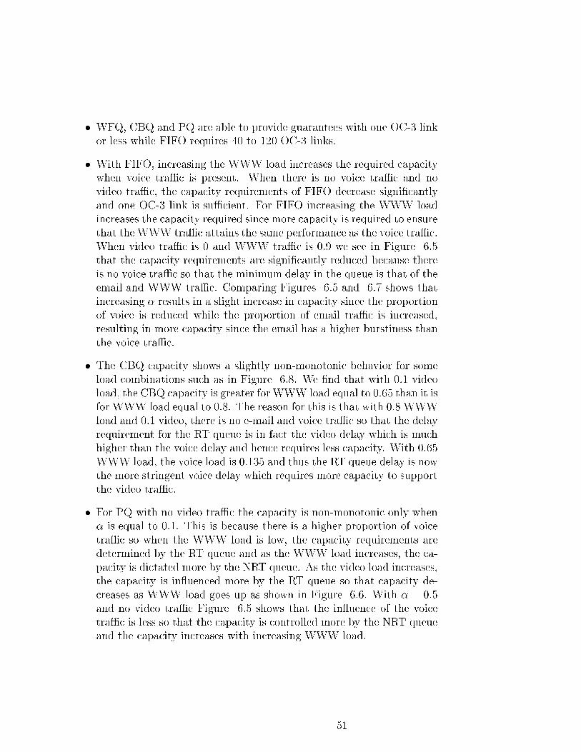
� WFQ, CBQ and PQ are able to provide guarantees with one OC-3 link

or less while FIFO requires 40 to 120 OC-3 links.

� With FIFO, increasing the WWW load increases the required capacity

when voice traÆc is present. When there is no voice traÆc and no

video traÆc, the capacity requirements of FIFO decrease signi�cantly

and one OC-3 link is suÆcient. For FIFO increasing the WWW load

increases the capacity required since more capacity is required to ensure

that the WWW traÆc attains the same performance as the voice traÆc.

When video traÆc is 0 and WWW traÆc is 0.9 we see in Figure 6.5

that the capacity requirements are signi�cantly reduced because there

is no voice traÆc so that the minimum delay in the queue is that of the

email and WWW traÆc. Comparing Figures 6.5 and 6.7 shows that

increasing � results in a slight increase in capacity since the proportion

of voice is reduced while the proportion of email traÆc is increased,

resulting in more capacity since the email has a higher burstiness than

the voice traÆc.

� The CBQ capacity shows a slightly non-monotonic behavior for some

load combinations such as in Figure 6.8. We �nd that with 0.1 video

load, the CBQ capacity is greater forWWW load equal to 0.65 than it is

for WWW load equal to 0.8. The reason for this is that with 0.8 WWW

load and 0.1 video, there is no e-mail and voice traÆc so that the delay

requirement for the RT queue is in fact the video delay which is much

higher than the voice delay and hence requires less capacity. With 0.65

WWW load, the voice load is 0.135 and thus the RT queue delay is now

the more stringent voice delay which requires more capacity to support

the video traÆc.

� For PQ with no video traÆc the capacity is non-monotonic only when

� is equal to 0.1. This is because there is a higher proportion of voice

traÆc so when the WWW load is low, the capacity requirements are

determined by the RT queue and as the WWW load increases, the ca-

pacity is dictated more by the NRT queue. As the video load increases,

the capacity is in uenced more by the RT queue so that capacity de-

creases as WWW load goes up as shown in Figure 6.6. With � = 0:5

and no video traÆc Figure 6.5 shows that the in uence of the voice

traÆc is less so that the capacity is controlled more by the NRT queue

and the capacity increases with increasing WWW load.

51

WFQ CBQ PQ 0

0.5

1Link Capacity with Video = 0%

Link

Cap

acity

(x

OC

−3)

WWW Load = 0.05WWW Load =0.275WWW Load = 0.5WWW Load =0.725WWW Load = 0.9

WFQ CBQ PQ FIFO0

20

40

60

80

100

120

140

Link

Cap

acity

(N

umbe

r of

OC

3 lin

ks)

Figure 6.7: Capacity Require-

ment with no Video (� = 0:1)

WFQ CBQ PQ 0

0.5

1Link Capacity with Video = 10%

Link

Cap

acity

(x

OC

−3)

WWW Load =0.05WWW Load =0.25WWW Load =0.45WWW Load =0.65WWW Load = 0.8

WFQ CBQ PQ FIFO0

20

40

60

80

100

120

Link

Cap

acity

(N

umbe

r of

OC

3 lin

ks)

Figure 6.8: Capacity Require-

ment with 10% Video(� = 0:1)

6.2.3 Delay Performance with changes in load

The goal of this analysis was to explore the ability of the three schemes to

provide acceptable delay QoS guarantees when the traÆc submitted exceeded

the traÆc for which the network was designed. We considered two scenarios:

one in which voice was the dominant traÆc type and another in which WWW

traÆc was dominant. For each scenario, the capacity required by each of the

four schemes was calculated using the procedures in Section 6.1. The number

of sources, the link capacities and the delay performance are collectively

referred to as the design point. For each scenario, the volume of either voice

or WWW traÆc was varied and the delay for each traÆc type was calculated

using the design point capacities. We note that in practice call admission

procedures would be used to restrict the number of ows admitted but since

we are testing the sensitivity of the traÆc handling schemes we assume no

call admission control. Instead we consider two approaches for bandwidth

allocation under WFQ. In the �rst method which we call WFQ1, an increase

in the traÆc of a particular class is handled by re-distributing the bandwidth

share of that class (as determined by the load wk at the design point) equally

among the sources (old and new). In the second approach called WFQ2, an

increase in voice traÆc is accommodated by "stealing" bandwidth from the

e-mail and WWW classes and giving this to the new voice traÆc to guarantee

the voice traÆc its delay QoS. Under WFQ2 an increase in WWW traÆc is

handled in the same way as with WFQ1. We present our results in the form

of plots of the ratio of actual delay to desired delay as a function of the %

change in voice or WWW load. The results obtained are presented in the

paragraphs that follow.

52

0 10 20 30 40 50 60 70 80 900.9

1

1.1

1.2

1.3

1.4

1.5

1.6

1.7

1.8

1.9Variation in Voice Delay for Network Dominated by Voice

% Increase in Voice

Act

ual D

elay

/Del

ay b

ound

WFQ1WFQ2CBQ PQ FIFO

Figure 6.9: Variation in Voice

Delay with increase in Voice

load

0 10 20 30 40 50 60 70 80 900

0.2

0.4

0.6

0.8

1

1.2

1.4

1.6

1.8Variation in WWW Delay for Network Dominated by Voice

% Increase in Voice

Act

ual D

elay

/Del

ay b

ound

WFQ1WFQ2CBQ PQ FIFO

Figure 6.10: Variation in

WWW Delay with increase in

Voice load

� Network dominated by voice with increase in voice traÆc

Figure 6.9 shows the results obtained for a design point with voice

as the dominant traÆc type corresponding to w1 = 40%, w2 = 10%,

w3 = 15% and w4 = 15% with changing voice traÆc. In this case the

delay guarantees provided by WFQ1 to voice increase as the voice load

increases since less and less bandwith is now available to each individual

connection. CBQ and PQ delay guarantees for voice also increase as

the voice load increases. WFQ2 and FIFO delay guarantees are not

signi�cantly a�ected by the increased voice traÆc. Under WFQ1 the

delay guarantees of video, email and WWW are not impacted by the

increased voice traÆc while under CBQ and PQ, the delays for video are

increased but are still within the speci�cations. Under WFQ2 Figure

6.10 shows that the delays for email and WWW are increased since

bandwidth is taken from them to support the increase in voice traÆc.

We note that for email delay guarantees are violated for an increase

in voice traÆc greater than 83% while for WWW the violation occurs

at an increase of 50%. The impact of the stolen bandwidth is more

pronounced on the WWW traÆc because of its higher burstiness.

� Network dominated by voice with increase in WWW traÆc

When the WWW traÆc increases Figure 6.11 shows that FIFO is not

able to provide the delay guarantees required by voice while all other

traÆc types are una�ected. For WFQ, CBQ and PQ, the voice traÆc

is isolated from the WWW traÆc and there is no impact on the voice

delay. CBQ delay for email is a�ected by the increase in WWW traÆc

53

and the delay required by email is violated by the slightest increase in

WWW traÆc as shown in Figure 6.12. With PQ, the delay of email

and WWW increases with increasing WWW load but is still within

their speci�cations. For all four schemes, the delay requirements of

video traÆc are not a�ected by the increase in WWW traÆc. Thus

when we increase the WWW traÆc, FIFO is now the most sensitive

and we cannot meet the delay objectives for voice.

0 10 20 30 40 50 60 70 80 900.9

1

1.1

1.2

1.3

1.4

1.5

1.6Variation in Voice Delay for Network Dominated by Voice

% Increase in WWW

Act

ual D

elay

/Del

ay b

ound

WFQ1WFQ2CBQ PQ FIFO

Figure 6.11: Variation in Voice

Delay with increase in WWW

load

0 10 20 30 40 50 60 70 80 900

0.2

0.4

0.6

0.8

1

1.2

1.4

1.6Variation in WWW Delay for Network Dominated by Voice

% Increase in WWW

Act

ual D

elay

/Del

ay b

ound

WFQ1WFQ2CBQ PQ FIFO

Figure 6.12: Variation in

WWW Delay with increase in

WWW load

� Network dominated by WWW with increase in voice traÆc

The impact on the voice and video delay is the same as in the case

of the network dominated by voice. For email and WWW, the delay

guarantees are violated under PQ at a lower value of increase in voice

load (10%) due to the increased WWW load.

� Network dominated by WWW with increase in WWW traÆc

In this case video is the only traÆc type that has its delay guarantees

met under any scheme. For voice, all schemes fail to meet the delay

requirements while for email CBQ and PQ fail to meet the guarantees.

For WWW CBQ and PQ also fail to meet the delay objectives while

WFQ fails when the increase in WWW load is greater than 50%.

The picture emerging from these results is that the traÆc handling schemes

are both sensitive to the type of traÆc that dominates the network at the

design point as well as to the type of traÆc that increases the load on the

54

network. In general FIFO is the least sensitive to increases in voice traÆc and

the most sensitive to increases in WWW traÆc when considering the delay

objectives of voice. WFQ, CBQ and PQ are all sensitive to increases in the

voice load and if the goal is to maintain the delay objectives of voice at all

costs, the use of a scheme like WFQ2 can achieve this with a corresponding

exponential increase in the delay of e-mail and WWW traÆc. The value

of these results is best demonstrated by taking into account the permissible

variances in the delay objectives which means using statistical objectives

as opposed to deterministic ones. The use of statistical delay objectives is

discussed in Chapter 10.

6.2.4 Required Capacity with Projections on TraÆc

Growth

In this part of the analysis we calculate the capacity required to support

yearly projections on growth in voice and WWW traÆc. Current industry

estimates are that voice traÆc on the Internet will grow at a rate of 5-15%

each year. The trend in WWW traÆc has been almost a 100% increase in

traÆc per year [19]. We assumed the two scenarios in Section 6.2.3 of either

voice or WWW being the dominant traÆc type. Using the same procedures

as before, we calculated the capacity required over a 5 year period assuming

a 15% growth in voice traÆc per year and a 100% growth in WWW traÆc

per year. The results obtained are shown in Figures 6.13 and 6.14 with the

capacity expressed in terms of the minimum number of OC-3 links.

For the network dominated by voice we �nd from Figure 6.13 that the

capacity required for WFQ increases to 4 times the initial capacity, CBQ

by a factor of 3 and PQ by a factor of 2 after the 5 year period. FIFO

capacity increases to 8 times the initial capacity, reaching 400 OC-3 links

after 5 years. We note that the rate of increase in capacity for WFQ, CBQ

and PQ is the same as evidenced by the slopes of the plots. The di�erence

is that for WFQ the increase in capacity occurs after the second year while

for CBQ and PQ the increase in capacity occurs after the third and fourth

years respectively. For FIFO the increase in capacity is more exponential

than linear and capacity increases right after the �rst year. When we start

with a network dominated by WWW traÆc as in Figure 6.14, the capacity

of WFQ increases by a factor of 7 while CBQ and PQ capacity increases by

5 after the 5 year period. FIFO capacity increases by a factor of 13. In both

cases FIFO is a�ected the most by the increase in traÆc especially since we

are increasing the volume of WWW traÆc by a substantial amount.

55

1 2 3 4 51

2

3

4

Projected Capacity with 15%/Yr increase in Voice and 100%/Yr increase in WWWNetwork Dominated by Voice

Year

Num

ber

of O

C−

3 Li

nks

WFQCBQPQ

1 2 3 4 50

100

200

300

400

500

Year

Num

ber

of O

C−

3 Li

nks

FIFO

Figure 6.13: Network Capacity

with Projections on Voice and

WWW TraÆc

1 2 3 4 51

2

3

4

5

6

7

Projected Capacity with 15%/Yr increase in Voice and 100%/Yr increase in WWWNetwork Dominated by WWW

Year

Num

ber

of O

C−

3 Li

nks

WFQCBQPQ

1 2 3 4 50

200

400

600

800

1000

1200

YearN

umbe

r of

OC

−3

Link

s

FIFO

Figure 6.14: Network Capacity

with Projections on Voice and

WWW TraÆc

To complete the picture we considered a hypothetical future situation in

which the growth of WWW traÆc is 15% and that of voice is 100%. This

corresponds to the hypothesis that eventually growth in voice traÆc will out-

pace growth in WWW traÆc. The projections on capacity in this case are

shown in Figures 6.15 and 6.16.

We �nd in this case that for a Voice-dominated network, CBQ and PQ

capacity increase the least by a factor of 4 while WFQ increases by a factor

of 7. FIFO capacity increases by only a factor of 1.5. For a WWW-dominated

network, WFQ capacity increases by a factor of 4 and CBQ and PQ by 2

while the FIFO capacity increases by a factor of 1.6. We conclude that WFQ

is a�ected more by the volume of voice traÆc than the aggregate schemes

while FIFO is a�ected most by the volume of WWW traÆc when voice traÆc

is present in the network.

Comparing Figures 6.13 and 6.15 we observe that for FIFO a 100%

increase in WWW requires more capacity than a 100% increase in voice

while for WFQ, CBQ and PQ the reverse is true. The FIFO results can

be attributed to the higher burstiness of WWW coupled with the much

lower delay QoS for voice. This would lead us to conclude that FIFO is more

sensitive to WWW traÆc while WFQ, CBQ and PQ are more sensitive to the

voice traÆc. We also note that a network dominated by WWW requires more

than 2 times the capacity of one dominated by voice under FIFO whereas

under WFQ, CBQ and PQ the e�ect is reversed. This again points to FIFO

being more sensitive to WWW traÆc whereas the other schemes are more

56

1 2 3 4 51

2

3

4

5

6

7

Projected Capacity with 100%/Yr increase in Voice and 15%/Yr increase in WWWNetwork Dominated by Voice

Year

Num

ber

of O

C−

3 Li

nks

WFQCBQPQ

1 2 3 4 540

45

50

55

60

65

Year

Num

ber

of O

C−

3 Li

nks

FIFO

Figure 6.15: Network Capacity

with Projections on Voice and

WWW TraÆc

1 2 3 4 51

2

3

4

Projected Capacity with 100%/Yr increase in Voice and 15%/Yr increase in WWWNetwork Dominated by WWW

Year

Num

ber

of O

C−

3 Li

nks

WFQCBQPQ

1 2 3 4 580

90

100

110

120

130

140

YearN

umbe

r of

OC

−3

Link

s

FIFO

Figure 6.16: Network Capacity

with Projections on Voice and

WWW TraÆc

sensitive to the voice traÆc.

6.2.5 Capacity Requirements with Varying Delay Guar-

antees

In this section we look at how the value of delay guarantees required by

voice and WWW impact the capacity requirements. We used load values of

w1 = 0:4, w2 = 0:1, w3 = 0:15 and w4 = 0:15 and obtained the capacity

required by the four traÆc handling schemes for di�erent values of voice and

WWW delays. We present our results for CBQ, PQ and FIFO in terms of

the ratio of their capacities to the WFQ capacity. In Table 6.2 we show

results for varying voice delay.

Voice Delay(sec) CWFQ(Mbps) C

CBQ=C

WFQCPQ=C

WFQCFIFO

=CWFQ

0.001 121.23 1.08 0.88 99.6

0.0015 121.23 0.86 0.67 66.5

0.002 121.74 0.76 0.57 49.7

0.0025 121.64 0.7 0.5 39.8

0.003 121.57 0.66 0.46 33.29

Table 6.2: Capacity as a function of Voice Delay

From the table we see that the ratio of CBQ, PQ or FIFO capacity to

WFQ capacity decreases as the voice delay increases. PQ has the smallest

57

ratios followed by CBQ and FIFO has the largest ratios. The FIFO ratios

are inversely related to the voice delays - tripling the delay from 0.001 to

0.003 causes the ratio (and hence FIFO capacity) to decrease by a factor of

3. Table 6.3 shows results when WWW delay is varied. One noticeable

WWW Delay(sec) CWFQ(Mbps) C

CBQ=C

WFQCPQ=C

WFQCFIFO

=CWFQ

0.025 112.3 2.3 1.8 21.8

0.05 119 1.5 1.01 23.3

0.1 119 1.1 0.6 27.4

0.15 121.3 0.99 0.56 32.3

0.2 120.8 0.93 0.56 36.5

0.25 121.8 0.89 0.56 41.63

0.375 121.74 0.83 0.56 49.74

0.5 121.74 0.76 0.56 49.74

0.625 121.74 0.76 0.56 49.74

0.75 121.74 0.76 0.56 49.74

Table 6.3: Capacity as a function of WWW Delay

di�erence between Tables 6.2 and 6.3 is that the WFQ capacity is more

signi�cantly a�ected by the WWW delay than it is by the voice delay. This

is because the results in Table 6.2 have the WWW delay equal to 0.5sec

for which value the guaranteed rate is the average rate � while for values of

WWW delay less than 0.25sec in Table 6.3 the guaranteed rate is dependent

on the delay and is greater than the average rate. Thus a smaller delay value

requires a larger guaranteed rate which limits the number of WWW ows

that can be carried while not exceeding the 0.15 load limit. For CBQ and

PQ, the ratios are greater for smaller values of delay since more capacity is

required to support the NRT queue. For FIFO we see the reverse e�ect since

at smaller WWW delay values there are fewer WWW ows which reduces

the total burstiness in the FIFO queue and minimizes the capacity required

to achieve the voice delay requirements. We note that for each scheme there

is a value of WWW delay above which the delay ceases to have an impact on

the capacity. For WFQ and FIFO this is 0.25sec since the guaranteed rate is

constant and thus the number of WWW ows remains constant. For CBQ

it is 0.5 because the e-mail delay is 0.5sec and with WWW delays greater

than 0.5, the NRT queue capacity is determined by the e-mail delay. For

PQ the capacity does not change above 0.15sec because the capacity is being

determined by the RT queue.

58

6.2.6 Capacity Requirements with Varying Burstiness

In this section we examine how varying the input burstiness a�ects the ca-

pacity requirements. We varied the burstiness by quantifying the burstiness

in terms of the time taken to transmit a burst at each traÆc type's average

rate. This would allow us to obtain di�erent levels of burstiness while using

consistent terms of reference. We conducted analyses for di�erent burst du-

rations ranging from 10ms to 100ms. Figure 6.17 shows results for a burst

duration of 10ms for each traÆc type.

WFQ CBQ PQ 0

0.5

1Link Capacity with Video = 20% Burst lengths = 10msec

Link

Cap

acity

(x

OC

−3)

Voice Load = 0.05Voice Load =0.225Voice Load = 0.4Voice Load =0.575Voice Load = 0.7

WFQ CBQ PQ FIFO0

0.5

1

1.5

2

2.5

3

3.5

4

Link

Cap

acity

(N

umbe

r of

OC

3 lin

ks)

Figure 6.17: Link Capacity

with 10ms bursts

WFQ CBQ PQ 0

0.5

1Link Capacity with Video = 20% Burst lengths = 10,50,100,100msec

Link

Cap

acity

(x

OC

−3)

Voice Load = 0.05Voice Load =0.225Voice Load = 0.4Voice Load =0.575Voice Load = 0.7

WFQ CBQ PQ FIFO0

5

10

15

20

25

30

35

Link

Cap

acity

(N

umbe

r of

OC

3 lin

ks)

Figure 6.18: Link Capacity

with varying burst sizes

This corresponds to burst sizes of 80 bytes for voice, 1875 bytes for video,

160 bytes for e-mail and 1250 bytes for WWW. We note in this case that

the capacity requirements are of the same order of magnitude with FIFO

requiring at most 4 times the capacity of WFQ, CBQ and PQ. In Figure 6.18

we used burst durations of 10ms for voice, 50msec for video and 100msec for

email and WWW. This corresponds to burst sizes of 80 bytes for voice, 9375

bytes for video, 1600 bytes for e-mail and 12500 bytes for WWW. We see

now that the gap between FIFO and the other schemes has widened and that

FIFO now requires at most 30 times more capacity. Comparing these results

with previous results based on the default parameters in Table 5.2, which

correspond to burst durations of 8msec for voice, 42.7msec for video, 192msec

for email and 327.7msec for WWW, we see that the increase in burstiness of

e-mail and WWW a�ects FIFO the most and the di�erence in capacity with

the default parameters is at most 85. These results demonstrate in part that

as the traÆc types become less and less homogeneous in their burstiness

parameters, the di�erence in capacity between FIFO and the other three

59

schemes widens whereas WFQ, CBQ and PQ are not a�ected much by the

disparity in burst sizes.

6.3 Summary

In this chapter we have developed and used an analytic method for evaluating

the capacity requirements of di�erent traÆc handling schemes. We focused

on the case of a single link and have obtained results that demonstrate several

ways in which the analysis can be used. We have looked at the impact of

the traÆc mix, the e�ect of growth in network traÆc both on the delay

performance and annual traÆc requirements and we have considered how

the burstiness parameter a�ects the capacity requirements. Our key �nding

is that there is no signi�cant di�erence between WFQ, CBQ and PQ on

the basis of capacity required to provide the same delay QoS. For FIFO we

have seen that the capacity requirements are in uenced by the aggregate

burstiness and the most stringent delay QoS and only when the aggregate

burstiness is very low do we get FIFO capacity that is the same order of

magnitude as the other three schemes. In the next section we extend our

analysis to carrier sized networks.

60

Chapter 7

Network Analysis

In this chapter we provide the analysis and methodology needed to evaluate

traÆc handling schemes in carrier-sized networks. We begin by de�ning the

topology of carrier-sized networks and then consider what approaches can be

used to perform the analysis. Next we develop the analysis for the edge and

core portions of the network after which we provide some numerical results.

7.1 General Network Topology

We consider a network architecture that has two distinct hieararchical layers

- an edge and a core - as shown in Figure 7.1. The core is the backbone of

the network and consists of high-speed switching elements. The edge portion

of the network provides access to the core network and serves to aggregate

traÆc into the network core. In some cases the edge is divided into two

layers: an access layer and a distribution layer [34].

The parameters and notation we use to describe a topology are:

� TraÆc Handling Scheme X - Y - X where X is the traÆc handling

scheme in the edge of the network and Y is the traÆc handling scheme

in the core.

� Number of core nodes Ncore

� Number of edge nodes per core node Nedge

� Reference capacity of edge links Cedge (homogeneous across the net-

work)

61

E

C

E

E

EE C

C C

E

E

E

Core LinkEdge LinkEdge Node

Core Node

Figure 7.1: Carrier Topology

� Core Connectivity Matrix A

This matrix describes the way in which the core nodes are connected.

For Ncore core nodes, the matrix is Ncore x Ncore and has elements aijwhere aij = 1 if a link exists from core node i to core node j and 0

otherwise. Note that links are unidirectional.

� Core TraÆc Distribution Matrix Tk

This matrix describes how the traÆc belonging to a particular type k,

incident at a core node is distributed to the destination core nodes in

the network. There is one matrix for each traÆc class and each matrix

is of size Ncore x Ncore. The elements of the matrix are fractions of

the per-class traÆc destined for a speci�c core node. For example let

Ncore = 3 and suppose �k is the distribution matrix for voice traÆc.

Then �12k = 0:5 means 50% of voice traÆc incident at core node 1 is

destined for core node 2 etc.

� TraÆc Allocation

The traÆc allocation for each traÆc type denoted wk, is speci�ed with

respect to each edge link so that it measures how much bandwidth on

a single edge-link has been allocated to a speci�c type. More precisely,

62

the allocation is the fraction of the edge link capacity assigned with

0 � wk < 1 andP

k wk < 1. It is used together with the guaranteed

rate to determine how many sources of each type may be supported on

one edge link. The total allocation is denoted wT and is equal toPwk.

7.2 Analysis of Network Capacity Require-

ments

As noted in Section 4.2, in performing the end-to-end analysis we can either

analyze each node separately and accumulate delays [23, 24] or we can

analyze the end-to-end path as a whole [62, 63]. The �rst approach can

lead to very loose bounds on delay however the second approach is applicable

only when all the nodes in the network are rate-guaranteeing and a minimum

guaranteed rate can be identi�ed. Since we are using traÆc handling schemes

that vary in their ability to provide rate guarantees, the analysis of the end-

to-end path will be done in the following manner [11, 90, 91]:

1. divide the path into regions containing rate-guaranteeing and non-rate

guaranteeing segments

2. analyze the non-rate guaranteeing segments by accumulating delays

additively

3. analyze the rate-guaranteeing segments using the path approach

4. sum the delays in the rate-guaranteeing and non-rate guaranteeing seg-

ments to obtain the end-to-end delays

For the edge-to-core node ratio, we calculate the number of edge nodes per

core node based on a �xed total external load on the core and assign traÆc

to each edge node to meet a prescribed utilization level on the edge links.

For rate-guaranteeing schemes such as WFQ there are two possibilities for

bandwidth allocation in the network: core nodes allocate same bandwidth as

edge nodes to each connection or core nodes allocate more bandwidth than

edge nodes. We will use the �rst approach for simplicity which will mean

that the delays in the core are the same as in the edge. The second approach

may be more useful when optimizing the delay budget since we can reduce

the delays in the core by allocating more bandwidth.

Since the goal is to compare the network capacity required by di�erent

traÆc handling schemes, we must ensure that there is a uniform basis for

63

comparison. As with the single node case we use a network with WFQ in

both the edge and core as the reference. We will refer to this network as

the reference network and use the notation WFQ� to distinguish it from

other networks. The approach is thus to calculate the amount of traÆc that

can be supported in a WFQ� network and compare the capacity required to

support the same traÆc for various combinations of traÆc handling schemes

in the edge and core.

7.3 Preliminary Equations and Parameters

In addition to the parameters introduced in Section 6 we de�ne the following

parameters:

� MT - maximum number of nodes traversed by any ow in the network

� M - maximum number of core nodes traversed by any ow in the net-

work

� DE2Ek - maximum end-to-end delay for traÆc of type k

� Dk - maximum delay per node for traÆc of type k. We assume that

the delays are uniformly distributed over the nodes to give:

Dk =DE2Ek

MT

Using Equation 4.11, we calculate the guaranteed rate with WFQ* gWFQ�k

as :

gWFQ�k = max

(�k;

�kMT

+ Lk

Dk

)(7.1)

where we have again assumed that the factor Lmax

Cin Equation 4.11 is

negligible. From Equation 7.1 we observe that the value assigned to gWFQ�k

will depend on the maximum number of nodes traversed and we can �nd the

critical value of MT by solving the inequality:

64

�k ��kMT

+ Lk

Dk

(7.2)

�k � (�k +MT � Lk)DE2Ek

(7.3)

This gives

M�T =

�k �DE2Ek � �k

Lk(7.4)

So, when the number of nodes traversed is less than M�T , g

WFQ�k = �k and

when the number of nodes traversed is greater than M�T , g

WFQ�k =

�kMT

+Lk

Dk.

This value of MT will become important when we compare capacity require-

ments for networks of varying size. The number of sources of each type that

can be supported at an edge node using WFQ* is given by:

Nk =

$wk � Cedge

gWFQ�k

%(7.5)

where Cedge is the edge link capacity and wk is the proportion of capacity on

the edge link allocated to traÆc of class k. We can now proceed to calculating

the edge and core capacity required to support this traÆc.

7.4 Edge Capacity Requirements

The analysis of capacity in the edge is similar to the Single-Node analysis

of Section 6 thus we will omit the details and present the equations. For

WFQ, the edge capacity is given by:

CWFQ�edge =

KXk=1

Nk � gWFQ�k

=KXk=1

wkCedge (7.6)

65

For CBQ and PQ with P classes/levels we have:

CCBQedge =

PXp=1

Xk2p

Nk�k + Lp

Dclass p

p = 1; 2; :::::::P (7.7)

CPQedge = max

p=1:::P

8<:

pXj=1

Xk 2 class j

Nk�k + Lmax(p)

Dclass p

+p�1Xj=1

Xk 2 class j

Nk�k

9=;(7.8)

For FIFO, the capacity is given by:

CFIFOedge =

KXk=1

Nk�k

Dmin

(7.9)

In the next section we explore how using di�erent mechanisms in the edge

and core a�ects the core capacity.

7.5 Core Capacity Requirements

The capacity required in the core for each scheme has the same general form

regardless of the mechanism in the edge. The key di�erentiating factor is the

change in burstiness for a given traÆc type induced by the delay in the edge.

Since edge capacities are calculated to meet the prescribed QoS objectives

for each class, we can assume that the edge delay will be bounded by the

per-node maximum delay Dk. For a WFQ core, using the traÆc distribution

matrices T k, the minimum required capacity on the link l(i; j) between the

core node-pair (i; j) is given by:

CWFQcore(i;j) = Nedge �

KXk=1

X(x;y)

�(x;y)k �Nx

k � gk (7.10)

f(x; y) : l(i; j) 2 Path(x; y)g

where �(x;y)k represents the distribution factors of ows between core nodes

(x; y) whose path Path(x; y) includes the link l(i; j) and Nxk is the number of

66

sources of class k whose edge node is attached to core node x. The value of

gk will depend on the traÆc handling in the edge: when the edge uses WFQ,

gk will be the same as gWFQ�k in Equation 7.1 and when the edge uses any

other mechanism, it will be:

gk = max

8<:�k;

�0

k

M+ Lk

Dk

9=; (7.11)

where M is the number of core nodes and �0k is the burstiness after passing

through the edge portion of the network which is given by:

�0k = �k + �kD

edgek (7.12)

Dedgek =

8><>:

Dk WFQ

minj2classpfDjg k 2 class p CBQ; PQ

minkfDkg FIFO

(7.13)

To calculate the core capacity with CBQ, PQ and FIFO, for each link l(i; j)

let:

�(i;j)k =

X(x;y)

�(x;y)k N

xk �k (7.14)

�(i;j)k =

X(x;y)

�(x;y)k N

xk �

h(x;y)k (7.15)

where f(x; y) : l(i; j) 2 Path(x; y)g. Note that h(x; y) is the number of

hops traversed by the traÆc before reaching link l(i; j) and �h(x;y)k is the asso-

ciated burstiness which will depend in part on the traÆc handling mechanism

used in the edge. To be more speci�c, �h(x;y)k will be given by:

�h(x;y)k =

(�0k + h(x; y) � �k �Dclass p 8 k 2 p for CBQ=PQ

�0k + h(x; y) � �k �Dmin for FIFO

(7.16)

with �0k de�ned as before.

Then by inverting Equations 4.13, 4.14, 4.15 the core bandwidth required

on link l(i; j) for each scheme is calculated as follows:

67

CCBQcore(i;j) = Nedge �

PXp=1

Xk2p

�k(i;j) + Lp

Dclass p

(7.17)

CPQcore(i;j) = Nedge � max

p=1::::P

8<:

pXm=1

Xk2 class m

�k(i;j) + Lmax(p)

Dclass p

+p�1Xm=1

Xk2 class m

�(i;j)k

9=; (7.18)

CFIFOcore(i;j) = Nedge �

KXk=1

�(i;j)k

Dmin

(7.19)

where we again assume the term (Lmax=C) in Equation 4.15 is negligible.

The equations obtained in this chapter for calculating capacity requirements

in edge-core networks are a new result and one of the key contributions of

this thesis. In the next section we use the analysis of this section to provide

numerical results on capacity requirements of the four schemes for di�erent

edge-core combinations.

68

7.6 Numerical Results for Network Analysis

7.6.1 Topology Construction

Carrier network topologies were constructed by varying the number of core

nodes and the number of core links per node. For a given core node value

Ncore, the number of links per core node nlink was varied according to:

nlink = 2; 3::::::; Ncore � 1

This resulted in (Ncore � 2) di�erent topologies per core node value. For

each value of Ncore and nlink, the core nodes were connected according to the

following algorithm:

� Number the core nodes from 1 to Ncore

� Connect the ith core node to core nodes i+1, i+2,...... i+nlink where

the addition is modulo Ncore. This means that the entries (i; i + 1),

(i; i+2),...... (i; i+ nlink) in the connectivity matrix would be set to 1.

An example of a 5 node topology with 3 links per core node is shown in

Figure 7.2. Thus a topology is uniquely identi�ed by the pair (Ncore; nlink).

C

C

C C

CFigure 7.2: Topology with 5 Core Nodes and 3 links per node

Note that the case when the number of links per core node is equal to

(Ncore � 1) is the familiar full-mesh topology. For each topology, we used

69

the same external load on the core network by �xing the total number of

edge nodes Nedge and setting the number of edge nodes per core node to

Nedge = Ntotaledge =Ncore where N

totaledge is the total number of edge nodes in the

network. We used a value of N totaledge = 60 for the results reported here. Once

a topology had been constructed, routes were set-up within the core using

Djikstra's shortest path algorithm [83]. The maximum number of hops in

the core was noted in each case and the mean number of hops hops was

calculated as:

hops =

PNroutesn=1 hops(n)

Nroutes

where Nroutes is the total number of routes and hops(n) is the number of

hops in the nth route.

7.6.2 Parameters

The end-to-end delay values used for each traÆc type are shown in Table

7.1.

TraÆc Type Delay (sec)

Voice 0.02

Video 0.05

E-mail 0.5

WWW 0.5

Table 7.1: Maximum End-to-End Delay for Edge-Core Analysis

TraÆc within the core was distributed symmetrically1 so that each core

node sends an equal amount of traÆc to every other core node and the

traÆc distribution matrix is speci�ed by:

Tij =

(1

(Ncore�1)i 6= j

0 i = j

We used a maximum load on each edge link (wT ) of 90%. Using the

procedures outlined in the methodology, the capacity required in the edge

1We ran some tests with random distribution of traÆc in the core but this did not have

a signi�cant impact on the results obtained.

70

and core for all possible combinations of edge-core traÆc handling schemes

was calculated for di�erent topologies with core nodes ranging from 3 to 20.

The results obtained are presented in the sections that follow.

7.6.3 Capacity Requirements with Symmetric TraÆc

Distribution

The purpose of this analysis was to �nd out how bandwidth requirements

of the four schemes are a�ected by changes in the voice and WWW load on

the edge links. We used three values of video load (0,0.1,0.2) and in one case

we varied the voice load while in the other case we varied the WWW load

within the limits of the maximum load wT . The remaining edge bandwidth

was equally divided between email and WWW for the �rst case and email

and voice for the second. For each load setting we used the reference all-

WFQ network to establish how many ows of each type could be handled by

the edge nodes and then calculated the core capacity. We then calculated

the capacity required to support the same ows using di�erent combinations

of edge and core traÆc handling schemes. We present our results in the form

of bar graphs that show the mean core link capacity stacked on top of the

mean edge capacity. We consider three di�erent aspects of the results: the

impact of edge traÆc handling, the impact of the network diameter and the

impact of network connectivity.

Impact of Edge TraÆc Handling

For this section we will use the speci�c case of 20 core nodes in a full-mesh

topology with a video load of 0.1 to illustrate the results. For this case, each

core node supports 3 edge nodes and each core node sends 5.2% (= 1=19) of

the total incoming traÆc to every other core node. For the reference WFQ

network, we thus expect the core link bandwidth to be at least (3 �OC3)=19which is 15.8% of an OC-3 link. Figure 7.3 shows the capacity required for

di�erent core schemes when WFQ is used in the edge and voice load is varied

while Figure 7.4 shows results for varying WWW load.

In these and subsequent �gures we show bar-graphs plotted on two separate

y-axes to allow for better observation of the WFQ, CBQ and PQ results. Due

to the di�erence in magnitude between FIFO and the other three schemes,

plotting all the results on the same scale as in the lower y-axis sometimes

masks the di�erences between WFQ, CBQ and PQ. In addition we have

combined the edge and core results on one graph to better illustrate the dif-

71

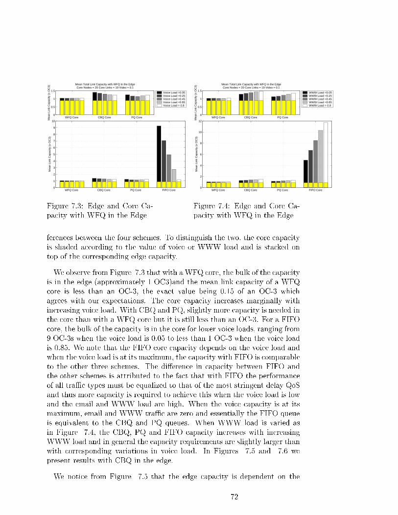
WFQ Core CBQ Core PQ Core 0

0.5

1

1.5

Mean Total Link Capacity with WFQ in the EdgeCore Nodes = 20 Core Links = 19 Video = 0.1

Mea

n Li

nk C

apac

ity (

x O

C3)

Voice Load =0.05Voice Load =0.25Voice Load =0.45Voice Load =0.65Voice Load = 0.8

WFQ Core CBQ Core PQ Core FIFO Core0

1

2

3

4

5

6

7

8

9

10

Mea

n Li

nk C

apac

ity (

x O

C3)

Figure 7.3: Edge and Core Ca-

pacity with WFQ in the Edge

WFQ Core CBQ Core PQ Core 0

0.5

1

1.5

Mean Total Link Capacity with WFQ in the EdgeCore Nodes = 20 Core Links = 19 Video = 0.1

Mea

n Li

nk C

apac

ity (

x O

C3)

WWW Load =0.05WWW Load =0.25WWW Load =0.45WWW Load =0.65WWW Load = 0.8

WFQ Core CBQ Core PQ Core FIFO Core0

2

4

6

8

10

12

Mea

n Li

nk C

apac

ity (

x O

C3)

Figure 7.4: Edge and Core Ca-

pacity with WFQ in the Edge

ferences between the four schemes. To distinguish the two, the core capacity

is shaded according to the value of voice or WWW load and is stacked on

top of the corresponding edge capacity.

We observe from Figure 7.3 that with a WFQ core, the bulk of the capacity

is in the edge (approximately 1 OC3)and the mean link capacity of a WFQ

core is less than an OC-3, the exact value being 0.15 of an OC-3 which

agrees with our expectations. The core capacity increases marginally with

increasing voice load. With CBQ and PQ, slightly more capacity is needed in

the core than with a WFQ core but it is still less than an OC-3. For a FIFO

core, the bulk of the capacity is in the core for lower voice loads, ranging from

9 OC-3s when the voice load is 0.05 to less than 1 OC-3 when the voice load

is 0.85. We note that the FIFO core capacity depends on the voice load and

when the voice load is at its maximum, the capacity with FIFO is comparable

to the other three schemes. The di�erence in capacity between FIFO and

the other schemes is attributed to the fact that with FIFO the performance

of all traÆc types must be equalized to that of the most stringent delay QoS

and thus more capacity is required to achieve this when the voice load is low

and the email and WWW load are high. When the voice capacity is at its

maximum, email and WWW traÆc are zero and essentially the FIFO queue

is equivalent to the CBQ and PQ queues. When WWW load is varied as

in Figure 7.4, the CBQ, PQ and FIFO capacity increases with increasing

WWW load and in general the capacity requirements are slightly larger than

with corresponding variations in voice load. In Figures 7.5 and 7.6 we

present results with CBQ in the edge.

We notice from Figure 7.5 that the edge capacity is dependent on the

72

WFQ Core CBQ Core PQ Core 0

1

2

3

Mean Total Link Capacity with CBQ in the EdgeCore Nodes = 20 Core Links = 19 Video = 0.1

Mea

n Li

nk C

apac

ity (

x O

C3)

Voice Load =0.05Voice Load =0.25Voice Load =0.45Voice Load =0.65Voice Load = 0.8

WFQ Core CBQ Core PQ Core FIFO Core0

2

4

6

8

10

12

Mea

n Li

nk C

apac

ity (

x O

C3)

Figure 7.5: Edge and Core Ca-

pacity with CBQ in the Edge

WFQ Core CBQ Core PQ Core 0

1

2

3

4

Mean Total Link Capacity with CBQ in the EdgeCore Nodes = 20 Core Links = 19 Video = 0.1

Mea

n Li

nk C

apac

ity (

x O

C3)

WWW Load =0.05WWW Load =0.25WWW Load =0.45WWW Load =0.65WWW Load = 0.8

WFQ Core CBQ Core PQ Core FIFO Core0

2

4

6

8

10

12

14

Mea

n Li

nk C

apac

ity (

x O

C3)

Figure 7.6: Edge and Core Ca-

pacity with CBQ in the Edge

voice load, being larger for smaller values of voice load which is attributed

to the correspondingly higher values of email and WWW load. The edge

capacity with CBQ is about twice that with a WFQ edge. We note that

the core capacity with WFQ, CBQ and PQ is less than or equal to 1 OC-3,

with CBQ having the larger core capacity. The FIFO core capacity follows

the same trend as with the WFQ edge, ranging from 10 to 1 OC-3. With

varying WWW load, Figure 7.6 shows that the CBQ edge capacity increases

with increasing WWW load as long as there is voice traÆc present. When

there is no voice (WWW = 0.8), the edge capacity drops slightly because

now the RT queue delay is determined by the video requirements which are

less stringent than the voice delay and thus less capacity is required for the

RT queue. The core capacities follow the same trend as with the WFQ edge.

With PQ in the edge, the variation in capacity for varying voice load is

shown in Figure 7.7. The key di�erence between having CBQ in the edge

versus PQ in the edge is the variation in edge capacity with voice load. We

note that the variation is non-monotonic, with the capacity decreasing with

increasing voice load up to a load of about 0.45 after which it starts to

increase with increasing voice load. When the WWW load is varied as in

Figure 7.8 the PQ edge capacity increases linearly with increasing WWW

load and the trend of core capacities is the same as with WFQ and CBQ.

When FIFO is used in the edge, the network capacity is dominated by the

edge capacity as shown in Figures 7.9 and 7.10.

With varying voice load as in Figure 7.9, the edge capacity depends greatly

on the voice load and ranges from 40 OC-3s when voice load is 0.05 to 2

73

WFQ Core CBQ Core PQ Core 0

1

2

3

Mean Total Link Capacity with PQ in the EdgeCore Nodes = 20 Core Links = 19 Video = 0.1

Mea

n Li

nk C

apac

ity (

x O

C3)

Voice Load =0.05Voice Load =0.25Voice Load =0.45Voice Load =0.65Voice Load = 0.8

WFQ Core CBQ Core PQ Core FIFO Core0

2

4

6

8

10

12

Mea

n Li

nk C

apac

ity (

x O

C3)

Figure 7.7: Edge and Core Ca-

pacity with PQ in the Edge

WFQ Core CBQ Core PQ Core 0

1

2

3

Mean Total Link Capacity with PQ in the EdgeCore Nodes = 20 Core Links = 19 Video = 0.1

Mea

n Li

nk C

apac

ity (

x O

C3)

WWW Load =0.05WWW Load =0.25WWW Load =0.45WWW Load =0.65WWW Load = 0.8

WFQ Core CBQ Core PQ Core FIFO Core0

2

4

6

8

10

12

14

Mea

n Li

nk C

apac

ity (

x O

C3)

Figure 7.8: Edge and Core Ca-

pacity with PQ in the Edge

WFQ Core CBQ Core PQ Core 0

20

40

60

Mean Total Link Capacity with FIFO in the EdgeCore Nodes = 20 Core Links = 19 Video = 0.1

Mea

n Li

nk C

apac

ity (

x O

C3)

Voice Load =0.05Voice Load =0.25Voice Load =0.45Voice Load =0.65Voice Load = 0.8

WFQ Core CBQ Core PQ Core FIFO Core0

5

10

15

20

25

30

35

40

45

50

Mea

n Li

nk C

apac

ity (

x O

C3)

Figure 7.9: Edge and Core Ca-

pacity with FIFO in the Edge

WFQ Core CBQ Core PQ Core 0

20

40

60

Mean Total Link Capacity with FIFO in the EdgeCore Nodes = 20 Core Links = 19 Video = 0.1

Mea

n Li

nk C

apac

ity (

x O

C3)

WWW Load =0.05WWW Load =0.25WWW Load =0.45WWW Load =0.65WWW Load = 0.8

WFQ Core CBQ Core PQ Core FIFO Core0

10

20

30

40

50

60

Mea

n Li

nk C

apac

ity (

x O

C3)

Figure 7.10: Edge and Core Ca-

pacity with FIFO in the Edge

74

OC-3s when the voice load is 0.8. With WFQ, CBQ and PQ cores, the

core capacity is of the order of 1 OC-3 whereas with a FIFO core the core

capacity ranges from 8 to 1 OC-3. With varying WWW load as in Figure

7.10, the FIFO edge capacity increases with increasing WWW load as long

as there is voice traÆc present. When there is no voice traÆc (WWW= 0.8),

the edge capacity starts to drop since the minimum delay is now the video

delay which is larger than the voice delay and thus less capacity is required

to provide delay guarantees. The FIFO core capacity also increases with

increasing WWW load whereas for WFQ, CBQ and PQ the core capacity is

not impacted much by the WWW load.

Core TraÆc Handling

WFQ CBQ PQ FIFO

Edge WFQ 107 201 144 1497

TraÆc CBQ 191 256 195 1818

Handling PQ 146 210 149 1700

FIFO 1212 1269 1224 2318

Table 7.2: Network Capacity for 20 Node Full-Mesh Network (in equivalent

OC3 links)

To illustrate the implications of these results in a network-wide sense, we

calculated the total network capacity for the 20 core node network in a full-

mesh con�guration for the speci�c case of voice load of 0.45 on the edge

links. The results are shown in Table 7.2 where the capacity is in multiples

of OC-3 capacity. Looking at the table we see that the all-WFQ network

requires the least network capacity while the use of FIFO in either the edge

or core requires large amounts of capacity. Using CBQ and PQ with WFQ

requires at most 2 times the capacity of the all-WFQ network. The general

conclusion to be drawn from these results is that any combination of WFQ,

CBQ and PQ in the edge and core will require capacity of the same order of

magnitude and on the basis of capacity requirements there is no signi�cant

di�erence between these three schemes.

Impact of Network Diameter

In this section we consider how the network diameter, measured in terms of

the maximum core hops traversed by a ow, a�ects the network capacity. We

use the cases of WFQ and FIFO in the edge for illustration since the CBQ

and PQ results are comparable to WFQ. In Table 7.3 we show the WFQ

capacity and the ratios of CBQ, PQ and FIFO capacity to WFQ capacity

for the case of WFQ in the edge with 20 core nodes. For all four schemes

75

Max Hops CWFQ (x OC3) C

CBQ=C

WFQCPQ=C

WFQCFIFO

=CWFQ

1 54 2.8 1.72 28.5

2 85 3.52 2.17 40.08

3 102 3.96 2.24 40.21

4 113 4.0 2.47 46.06

5 156 4.66 2.8 51.8

7 198 5.27 3.36 62.6

10 281 6.17 4.11 74.6

Table 7.3: Core Capacity as a function of Network Diameter for WFQ Edge

the capacity increases with network diameter although the rate of increase

is not the same. For instance with a WFQ core the capacity required by

a 10-hop network is 5.2 times that of a 1-hop (full-mesh) network while for

CBQ the factor is 11.5, for PQ it is 12.4 and for FIFO it is 13.6. When

FIFO is used in the edge, the results obtained are shown in Table 7.4. In

Max Hops CWFQ (x OC3) C

CBQ=C

WFQCPQ=C

WFQCFIFO

=CWFQ

1 77 1.74 1.15 15.5

2 99 2.5 1.57 22.12

3 117 3.13 1.83 28.65

4 145 3.8 2.15 34.4

5 171 4.4 2.4 39.8

7 213 5.3 2.84 49.9

10 297 6.67 3.58 62.54

Table 7.4: Core Capacity as a function of Network Diameter for FIFO Edge

this case the di�erence in capacity between a 10-hop and 1-hop network is

now 3.8 for WFQ, 14.8 for CBQ, 12 for PQ and 15.6 for FIFO. We note

however that for the same hop-count, the capacities with FIFO in the edge

are greater than with WFQ in the edge. Another way to look at the impact

of the network diameter is to consider the utilization in the core. We de�ne

the core utilization as:

� =Nedge

PKk=1Nk�k

Ccore

where Nedge is the total number of edge nodes, Nk is the number of ows

of type k, �k is the average rate of ows of type k and Ccore is the total

core capacity. We will use the results in Table 7.3 to discuss how network

76

diameter a�ects the utilization. For WFQ, the utilization ranges from 0.73 in

a full-mesh network to 0.14 in a 10-hop network. For CBQ the range is 0.25

to 0.02, for PQ it is 0.4 to 0.03 and for FIFO it is 0.025 to 0.001. In general

the utilization decreases with increasing hop count. This is because with a

�xed end-to-end delay budget, increasing the number of hops reduces the

maximum delay per node which results in more capacity per link to support

the same external load. For CBQ, PQ and FIFO there is the added e�ect of

accumulation in burstiness which increases the capacity requirements as the

network increases in diameter. For the type of topologies used here, small

hop counts are achieved by having more links per core node and intuitively

one would expect to have lower utilization when there are more links in the

network. The di�erence comes about because the capacity per link is much

higher in networks with more hops which makes the total network capacity

exceed that of networks with smaller hops, leading to reduced utilization. In

Chapter 9 we look at the relationship between capacity, delay and utilization

for CBQ, PQ and FIFO in more detail.

Impact of Network Connectivity

In this section we look at how the network connectivity a�ects the capacity

requirements. For a given number of core nodes, Ncore, the connectivity is

determined by the number of links per core node which ranges from 2 to

Ncore�1. With Ncore�1 links per node, the network is the highly-connected

full mesh topology with a maximum of 2 hops between edge nodes whereas

with 2 links per core node the network is poorly connected with a larger

number of hops between edge nodes. We use the cases of 5 and 20 core nodes

to illustrate the results for the case of FIFO in the edge. In Figures 7.11 and

7.12 we present results for a network with 5 core nodes and 2 and 4 links per

core node respectively.

Comparing the two graphs we notice that in a full-mesh topology with 4

links per core node, both the edge and core capacity are less than in the

topology with 2 links per core node. The reason for this is that in both

networks the end-to-end delay objective is the same so that the network

with more links per core node (smaller diameter) has a higher per-node delay

than that with fewer links per core node (larger diameter). A higher per-node

delay translates to less capacity required to achieve the delay objective.

Figures 7.13 and 7.14 show the results with 20 core nodes. Comparing the

two graphs we observe results similar to the 5 node case. A more interesting

comparison is to compare Figure 7.11 with 7.13 and Figure 7.12 with

7.14 which have the same number of links per node but di�erent number of

77

WFQ Core CBQ Core PQ Core 0

20

40

60

80

Mean Total Link Capacity with FIFO in the EdgeCore Nodes = 5 Core Links = 2 Video = 0.1

Mea

n Li

nk C

apac

ity (

x O

C3)

Voice Load =0.05Voice Load =0.25Voice Load =0.45Voice Load =0.65Voice Load = 0.8

WFQ Core CBQ Core PQ Core FIFO Core0

100

200

300

400

500

600

Mea

n Li

nk C

apac

ity (

x O

C3)

Figure 7.11: Edge and Core Ca-

pacity with FIFO in the Edge: 5

nodes poorly-connected

WFQ Core CBQ Core PQ Core 0

20

40

60

Mean Total Link Capacity with FIFO in the EdgeCore Nodes = 5 Core Links = 4 Video = 0.1

Mea

n Li

nk C

apac

ity (

x O

C3)

Voice Load =0.05Voice Load =0.25Voice Load =0.45Voice Load =0.65Voice Load = 0.8

WFQ Core CBQ Core PQ Core FIFO Core0

20

40

60

80

100

120

140

160

180

Mea

n Li

nk C

apac

ity (

x O

C3)

Figure 7.12: Edge and Core Ca-

pacity with FIFO in the Edge: 5

nodes highly-connected

WFQ Core CBQ Core PQ Core 0

50

100

150

200

Mean Total Link Capacity with FIFO in the EdgeCore Nodes = 20 Core Links = 2 Video = 0.1

Mea

n Li

nk C

apac

ity (

x O

C3)

Voice Load =0.05Voice Load =0.25Voice Load =0.45Voice Load =0.65Voice Load = 0.8

WFQ Core CBQ Core PQ Core FIFO Core0

200

400

600

800

1000

1200

Mea

n Li

nk C

apac

ity (

x O

C3)

Figure 7.13: Edge and Core Ca-

pacity with FIFO in the Edge:

20 nodes poorly-connected

WFQ Core CBQ Core PQ Core 0

20

40

60

Mean Total Link Capacity with FIFO in the EdgeCore Nodes = 20 Core Links = 19 Video = 0.1

Mea

n Li

nk C

apac

ity (

x O

C3)

Voice Load =0.05Voice Load =0.25Voice Load =0.45Voice Load =0.65Voice Load = 0.8

WFQ Core CBQ Core PQ Core FIFO Core0

5

10

15

20

25

30

35

40

45

50

Mea

n Li

nk C

apac

ity (

x O

C3)

Figure 7.14: Edge and Core Ca-

pacity with FIFO in the Edge:

20 nodes highly-connected

78

core nodes. We �nd that with 2 links per core node, the capacity with 20

core nodes is signi�cantly higher (by almost a factor of 2) than that with 5

core nodes for all the core schemes whereas with a full mesh topology the

capacity with 20 nodes is signi�cantly lower only for the FIFO core case.

In fact looking at the full mesh topologies we notice that the edge capacity

is the same irrespective of the number of nodes which is to be expected

since the network diameter is the same for all full-mesh topologies. In a

full-mesh topology, the FIFO core capacity with 20 nodes is less than with

5 core nodes because of the way in which traÆc is distributed inside the

core: recall that we are using a symmetric distribution in which the traÆc

sent from one core node to another is equal to the total load from the edge

divided by the number of core nodes minus 1. Thus with 20 nodes the traÆc

between nodes is less than with 5 core nodes. With 2 links per core node, the

edge capacity is signi�cantly greater with 20 core nodes since the network

diameter is larger and hence the delay per node is much smaller than with 5

core nodes, resulting in more capacity to meet delay objectives. The capacity

in the core is less with with 20 nodes again due to the symmetric distribution

of traÆc in the core.

7.6.4 E�ect of Projections on TraÆc Growth

Using procedures similar to those in Section 6.2.4, we investigate the impact

on core capacity of projected annual growth of 15% in voice traÆc and 100%

in WWW traÆc over a period of 5 years. We use a network with 20 core

nodes for illustration. Figure 7.15 shows the capacity required with WFQ

in the edge for the case of initial voice load of 40%, video 10%, email 15%

and WWW 15%. We note that the WFQ capacity increase by a factor of 2

to two OC-3 links after the 5 year period while CBQ and PQ both increase

by a factor of 4 although the CBQ capacity increases slightly faster than PQ

capacity between the second and third years. The FIFO capacity increases

the most by a factor of almost 9. With FIFO in the edge Figure 7.16 shows

the same trend as before for WFQ. The variation in CBQ and PQ capacity is

the same in this case and the capacity increases by a factor of 3. The FIFO

capacity increases by a factor of almost 14 although the net capacity is less

than with WFQ in the edge.

79

1 2 3 4 51

1.5

2

2.5

3

3.5

4

Projected Core Capacity with 15%/Yr Voice and 100%/Yr WWW growthNetwork Dominated by WWW Core Nodes = 20 Core Links = 19 Edge = WFQ

Year

Num

ber

of O

C−

3 Li

nks

WFQCBQPQ

1 2 3 4 50

20

40

60

80

100

Year

Num

ber

of O

C−

3 Li

nks

FIFO

Figure 7.15: Core Capacity for

20 node network with WFQ in

the Edge

1 2 3 4 51

1.5

2

2.5

3

Projected Core Capacity with 15%/Yr Voice and 100%/Yr WWW growthNetwork Dominated by WWW Core Nodes = 20 Core Links = 19 Edge = FIFO

Year

Num

ber

of O

C−

3 Li

nks

WFQCBQPQ

1 2 3 4 50

10

20

30

40

50

60

70

YearN

umbe

r of

OC

−3

Link

s

FIFO

Figure 7.16: Core Capacity for

20 node network with FIFO in

the Edge

7.6.5 Impact of Burstiness on Edge and Core Capacity

We tested the impact of burstiness on the edge and core capacity, focusing

on WWW burstiness for illustration. We varied the WWW burstiness to

give us values that ranged from 1 to 1000 times the burstiness of voice. We

used a 20-node full-mesh topology with �xed load of 40% voice, 15% video,

15% email and 15% WWW. For each burstiness value we calculated the edge

and core capacity and plotted these against the ratio of WWW to voice

burstiness. The results are shown in Figures 7.17 and 7.18.

We notice that for both the edge and core, the di�erence in capacity be-

tween FIFO and the other three schemes widens as the WWW burstiness

increases. This further reinforces the observation that the aggregate bursti-

ness is the key reason for the di�erence in capacity between FIFO and WFQ,

CBQ or PQ. For CBQ, the capacity also increases with increasing WWW

burstiness but the impact is not as great as in the FIFO case since the delay

requirements in the NRT (email and WW) queue are not as stringent as in

the FIFO queue. For PQ, the burstiness has no e�ect because the capacity

is solely determined by the RT queue.

80

200 400 600 800 1000 12000

5

10

15

20

25

Edge Link Capacity as a function of burstiness Core Nodes = 20 Core Links = 19

WWW burstiness/Voice burstiness

Num

ber

of O

C−

3 Li

nks

WFQ CBQ PQ FIFO

Figure 7.17: Edge Capacity as a

function of WWW burstiness

200 400 600 800 1000 12000

1

2

3

4

5

6

Core Link Capacity as a function of burstiness Core Nodes = 20 Core Links = 19 Edge = WFQ

WWW burstiness/Voice burstiness

Num

ber

of O

C−

3 Li

nks

WFQ CBQ PQ FIFO

Figure 7.18: Core Capacity as a

function of WWW burstiness

7.6.6 E�ect of Delay Ratios

In this section we look at the e�ect of voice and WWW delay requirements on

core capacity. We use a full mesh network with 10 core nodes for illustration

with a load of 40% voice, 10% video, 15% email and 15% WWW. Results

are presented in terms of the ratio of CBQ, PQ and FIFO core capacity to

WFQ core capacity. Table 7.5 shows the e�ect of the voice delay on core

capacity when WFQ is used in the edge. The WFQ capacity is not impacted

Voice Delay CWFQ(Mbps) C

CBQ=C

WFQCPQ=C

WFQCFIFO

=CWFQ

0.01 81.73 4.04 3.0 55.16

0.015 81.73 3.28 2.2 37.01

0.02 81.73 2.93 1.89 27.9

0.025 81.73 2.75 1.7 22.57

0.03 81.73 2.65 1.6 18.9

Table 7.5: Capacity as a function of Voice Delay with WFQ Edge

by the voice delay while for CBQ, PQ and FIFO the capacity decreases

with increasing voice delay. For CBQ and PQ the decrease in capacity is

because a larger value of voice delay requires less capacity to support the

RT queue. For FIFO, a larger value of voice delay also reduces the capacity

requirements of the entire queue. Note that for FIFO the relationship is linear

in that when the delay is increased by a factor of 3 the capacity reduces by

a factor 3. When FIFO is used in the edge, Table 7.6 shows that the WFQ

capacity increases with increasing voice delay. This is because as the voice

81

Voice Delay CWFQ(Mbps) C

CBQ=C

WFQCPQ=C

WFQCFIFO

=CWFQ

0.01 110 2.47 1.89 31.02

0.015 113 1.99 1.42 20.4

0.02 116 1.76 1.2 15

0.025 119 1.63 1.08 11.96

0.03 122 1.55 1.01 9.89

Table 7.6: Capacity as a function of Voice Delay with FIFO Edge

delay increases there is a corresponding increase in the burstiness of traÆc

through the FIFO edge and this requires more guaranteed bandwidth in the

WFQ core. For CBQ, PQ and FIFO, the capacity decreases with increasing

voice delay as before although the capacity requirements are now less than

with a WFQ edge. Increasing the WWW delay with a WFQ edge produces

results similar to the single-link case as shown in Table 7.7. With FIFO in

WWW Delay CWFQ(Mbps) C

CBQ=C

WFQCPQ=C

WFQCFIFO

=CWFQ

0.25 81 3.49 2.1 21.78

0.375 81 3.28 1.89 27.95

0.5 81 2.93 1.89 27.97

0.625 81 2.93 1.89 27.97

0.75 81 2.93 1.89 27.97

Table 7.7: Capacity as a function of WWW Delay with WFQ Edge

the edge, increasing the WWW delay reduces the WFQ capacity as shown

in Table 7.8. This is because a larger WWW delay reduces the guaranteed

WWW Delay CWFQ(Mbps) C

CBQ=C

WFQCPQ=C

WFQCFIFO

=CWFQ

0.25 122 1.96 1.15 11.42

0.375 124 1.84 1.13 14.2

0.5 116 1.76 1.2 15.1

0.625 113 1.83 1.25 15.69

0.75 111 1.86 1.27 16

Table 7.8: Capacity as a function of WWW Delay with FIFO Edge

rate for WWW traÆc. The CBQ, PQ and FIFO capacities do not change

for values of WWW delay above 0.375 - the change in ratios is due to the

changing WFQ capacity.

82

7.7 Summary

In summary the results of this chapter are:

� Any combination of WFQ, CBQ and PQ in the edge and core requires

capacity of the same order of magnitude and on the basis of capac-

ity there is no signi�cant di�erence between the three traÆc handling

schemes.

� With FIFO in the edge, the edge capacity dominates the total network

capacity and again there is no signi�cant di�erence between WFQ,

CBQ and PQ in the core.

� When voice and video are the only traÆc types in the network, there

is no di�erence between the four traÆc handling schemes.

� For the same delay budget and the same number of core nodes, increas-

ing the network connectivity increases the edge capacity but decreases

the core capacity.

� For the same delay budget and the same number of core links per node,

a larger network (more core nodes) requires more capacity due to the

increased network diameter.

� With WFQ in the edge, WFQ core capacity is not a�ected much by

increases in voice delay while increases in WWW delay decrease the

WFQ core capacity. CBQ, PQ and FIFO core capacity decrease with

increasing voice delay with WFQ in the edge

� With FIFO in the edge, WFQ core capacity increases with increasing

voice delay while CBQ, PQ and FIFO core capacity decreases.

� Increasing the WWW delay has no e�ect on WFQ core capacity with

a WFQ edge and reduces the WFQ core capacity when FIFO is used

in the edge.

� The aggregate burstiness is a critical factor for FIFO; as the aggre-

gate burstiness increases, the di�erence between FIFO capacity and

the other three schemes increases.

� With WFQ in the edge, CBQ, PQ and FIFO core capacity is not im-

pacted much by WWW delay while with FIFO in the edge, there is

a cuto� delay above which the core capacity does not change with in-

crease in WWW delay.

83

In the next chapter we look at how the analysis can be used to provide

bounds on the capacity requirements of the four traÆc handling schemes.

84

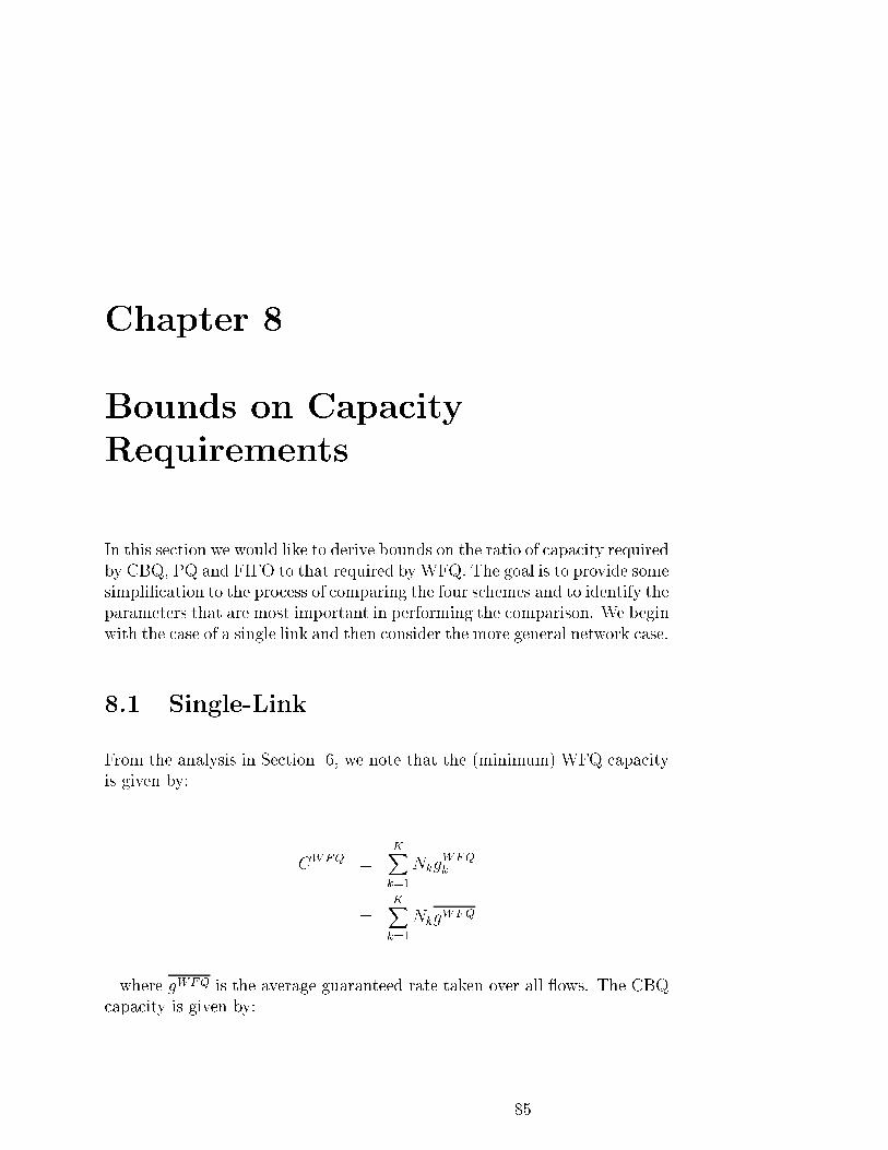
Chapter 8

Bounds on Capacity

Requirements

In this section we would like to derive bounds on the ratio of capacity required

by CBQ, PQ and FIFO to that required by WFQ. The goal is to provide some

simpli�cation to the process of comparing the four schemes and to identify the

parameters that are most important in performing the comparison. We begin

with the case of a single link and then consider the more general network case.

8.1 Single-Link

From the analysis in Section 6, we note that the (minimum) WFQ capacity

is given by:

CWFQ =

KXk=1

NkgWFQk

=KXk=1

NkgWFQ

where gWFQ is the average guaranteed rate taken over all ows. The CBQ

capacity is given by:

85

CCBQ =

PXp=1

Xk2p

Nk�k

Dclass p

+PXp=1

Lp

Dclass p

=KXk=1

Nk CBQ +

PXp=1

Lp

Dclass p

<

KXk=1

Nk CBQ +

PXp=1

Lp

Dmin

where CBQ is de�ned as:

CBQ =

PKk=1

Nk�kDk;pPK

k=1Nk

We thus obtain the ratio of CBQ to WFQ capacity as:

CCBQ

CWFQ<

CBQ

gWFQ+

PPp=1

LpDminPK

k=1NkgWFQ

(8.1)

The capacity with PQ is given by:

CPQ = max

p=1:::P

8<:

pXj=1

Xk 2 class j

Nk�k + Lmax(p)

Dclass p

+p�1Xj=1

Xk 2 class j

Nk�k

9=; (8.2)

= maxp=1:::P

8<:

pXj=1

Fj PQ(p) +

p�1Xj=1

Fj�H(p) +Lmax(p)

Dclass p

9=; (8.3)

where Fp is the number of ows in priority levels greater than or equal to

p, �H(p) is the average rate of all ows of priority greater than p and PQ(p)

is given by:

PQ(p) =

Ppj=1

Pk 2 class j

Nk�kDclass p

Fp(8.4)

The ratio of PQ to WFQ capacity is thus:

86

CPQ

CWFQ= max

p=1:::P

( PQ

gWFQ

Ppj=1 FjPKk=1Nk

+�H(p)

gWFQ

Pp�1j=1 FjPKk=1Nk

+ (8.5)

Lmax(p)

Dclass pPKk=1Nkg

WFQ

9>=>; (8.6)

For FIFO similar analysis yields:

CFIFO

CWFQ=

FIFO

gWFQ(8.7)

where FIFO is given by:

FIFO =

PKk=1

Nk�kDminPK

k=1Nk

(8.8)

We defer discussion of the nature of the bounds until after the next section

where we derive the bounds for the network case.

8.2 Edge-Core Network

In this section we look at how the core capacity with di�erent edge-core

traÆc handling mechanisms compares to that required by a network using

WFQ in both the edge and core. Speci�cally we obtain bounds on the ratio

of maximum core capacity for di�erent edge-core combinations compared to

an all WFQ network. The comparison is done for topologies having the same

number of core nodes and we make several assumptions on the traÆc in the

network:

� The load from the edge on each core node is the same so that Nmk = Nk

for each core node m

� TraÆc is distributed symmetrically within the core and the distribution

is the same for each traÆc type so that � i;jk = �k = � = 1=(Ncore � 1)

for all traÆc types k and all core nodes (i; j)

87

� There is an upper bound on the number of ows carried by a link (i; j)

that depends on the connectivity of the network which is given by:

Nmaxk (i; j) =

KXk=1

Nk � �max

�max = Linkflow(i; j) � �

where Linkflow(i; j) is the number of core source-destination pairs whose

traÆc is routed over link (i; j).

In the reference all-WFQ network, the maximum capacity on a core link is

found using Equation 7.10 to be:

CWFQ�core = Nedge �

KXk=1

Nk � gWFQ�k � �max (8.9)

This is the reference case and we will now consider maximum core capacity

for di�erent edge-core combinations.

8.2.1 WFQ Core

When the edge does not use WFQ, the maximumWFQ core capacity is given

by:

CWFQcore � Nedge�max

KXk=1

Nkgk (8.10)

where we recall that gk is given by:

gk = max

8<:�k;

�0

k

M+ Lk

Dk

9=; (8.11)

where �0k is the burstiness after passing through the edge portion of the

network de�ned in Equation 7.12 and M is the number of core nodes. Thus

the ratio of WFQ core capacity to the reference WFQ* network is:

88

CWFQcore

CWFQ�core

<g

gWFQ�(8.12)

8.2.2 CBQ Core

For CBQ using Equation 7.17 the maximum core capacity is given by:

CCBQcore � Nedge � �max

PXp=1

Xk2p

Nk�(M)k + Lp

Dclass p

� Nedge � �maxKXk=1

Nk�(M)k

Dk;p

+PXp=1

Lp

Dclass p

where �(M)k is the burstiness of a ow that traverses M core nodes which

is given by:

�(M)k = �

0k + (M � 1)�kDk;p

= �k + �kDedgek + (M � 1)�kDk;p

Substituting for �(M)k we have:

CCBQcore � Nedge � �max

KXk=1

Nk

"�k

gWFQ�k Dk;p

+�k

gWFQ�k

Dedgek

Dk;p

+ (M � 1)�k

gWFQ�k

#

+PXp=1

NedgeLp

Dclass p

< Nedge � �maxKXk=1

Nk CBQ +�CBQ + (M � 1)�+

PXp=1

NedgeLp

Dmin

where CBQ and �CBQ are de�ned as:

CBQ =

PKk=1

Nk�kDk;pPK

k=1Nk

(8.13)

89

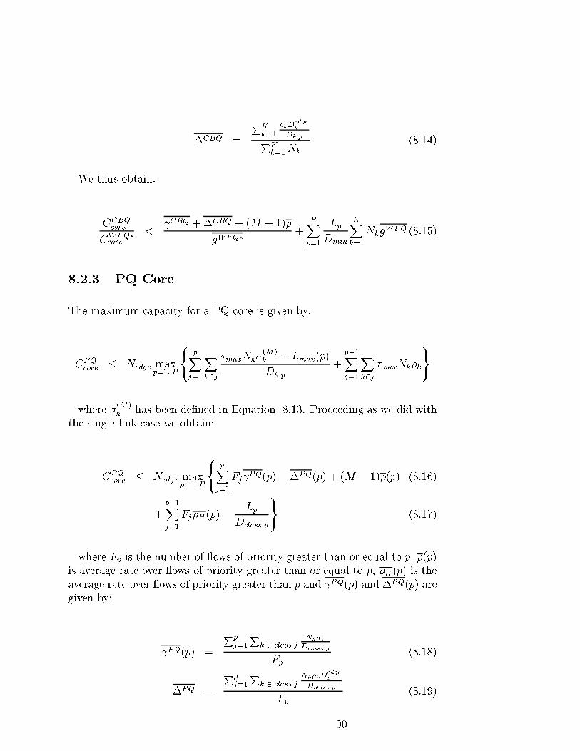
�CBQ =

PKk=1

�kDedgek

Dk;pPKk=1Nk

(8.14)

We thus obtain:

CCBQcore

CWFQ�core

< CBQ +�CBQ + (M � 1)�

gWFQ�+

PXp=1

Lp

Dmin

KXk=1

NkgWFQ (8.15)

8.2.3 PQ Core

The maximum capacity for a PQ core is given by:

CPQcore � Nedge max

p=1::P

8<:

pXj=1

Xk2j

�maxNk�(M)

k + Lmax(p)

Dk;p

+p�1Xj=1

Xk2j

�maxNk�k

9=;

where �(M)k has been de�ned in Equation 8.13. Proceeding as we did with

the single-link case we obtain:

CPQcore � Nedge max

p=1::P

8<:

pXj=1

Fj PQ(p) + �PQ(p) + (M � 1)�(p) (8.16)

+p�1Xj=1

Fj�H(p) +Lp

Dclass p

9=; (8.17)

where Fp is the number of ows of priority greater than or equal to p, �(p)

is average rate over ows of priority greater than or equal to p, �H(p) is the

average rate over ows of priority greater than p and PQ(p) and �PQ(p) are

given by:

PQ(p) =

Ppj=1

Pk 2 class j

Nk�kDclass p

Fp(8.18)

�PQ =

Ppj=1

Pk 2 class j

Nk�kDedge

k

Dclass p

Fp(8.19)

90

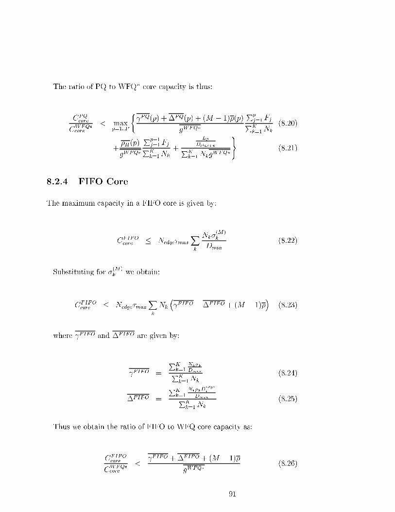
The ratio of PQ to WFQ* core capacity is thus:

CPQcore

CWFQ�core

< maxp=1::P

( PQ(p) + �PQ(p) + (M � 1)�(p)

gWFQ�

Ppj=1 FjPKk=1Nk

(8.20)

+�H(p)

gWFQ�

Pp�1j=1 FjPKk=1Nk

+

LpDclass pPK

k=1NkgWFQ�

9=; (8.21)

8.2.4 FIFO Core

The maximum capacity in a FIFO core is given by:

CFIFOcore � Nedge�max

Xk

Nk�(M)k

Dmin

(8.22)

Substituting for �(M)k we obtain:

CFIFOcore � Nedge�max

Xk

Nk

� FIFO +�FIFO + (M � 1)�

�(8.23)

where FIFO and �FIFO are given by:

FIFO =

PKk=1

Nk�kDminPK

k=1Nk

(8.24)

�FIFO =

PKk=1

Nk�kDedgek

DminPKk=1Nk

(8.25)

Thus we obtain the ratio of FIFO to WFQ core capacity as:

CFIFOcore

CWFQ�core

< FIFO +�FIFO + (M � 1)�

gWFQ�(8.26)

91

Looking at the bounds on capacity we notice that the CBQ, PQ and FIFO

bounds have certain elements in common. In each case the capacity is related

to a parameter which is determined by the ratio of burstiness within an

aggregate to the minimum delay requirements of that aggregate. For edge-

core networks, the delay in the edge in uences the capacity bounds and this

is captured by the parameter � which is a function of the ratio of edge delay

to core delay. We also note the factor (M-1) which captures the e�ect of the

network diameter on the capacity bounds. Since we know that the average

rate � is always less than or equal to the guaranteed rate g, we expect that the

ratios will be lower-bounded by (M-1). We have thus established bounds on

the capacity requirements that are related to the ratios of delay objectives of

the traÆc that is aggregated within the network. This is a new result which

is able to relate di�erences in capacity to di�erences in delay requirements.

In the next section we present some numerical results on the accuracy of the

bounds.

8.3 Numerical Results on Capacity Bounds

To demonstrate the use of the capacity bounds we will focus on the case of

a single link loaded with 40% voice, 10% video, 15% email and 15% WWW

and look at how the bounds change for varying voice delay. Starting with

CBQ we show in Table 8.1 the guaranteed rate and CBQ along with the

simpli�ed bounds obtained in this section and the bounds obtained from the

exact expressions in Chapter 7. We will refer to the bounds as the simple

and exact bounds respectively.

Voice Delay gWFQ CBQ=gWFQ CCBQ

=CWFQ

(sec) (Mbps) Simple Exact

0.001 0.45 0.99 1.25 1.08

0.0015 0.41 0.8 0.88 0.86

0.002 0.37 0.72 0.78 0.76

0.0025 0.34 0.66 0.71 0.7

0.003 0.31 0.64 0.68 0.66

Table 8.1: Ratio of CBQ to WFQ Capacity as a function of Voice Delay

We �nd that the simple bounds are accurate and we note that CBQ can

be used to provide reasonable estimates in the absence of information about

packet sizes. The results for PQ are shown in Table 8.2. We note that

for this particular case the PQ capacity is maximized by the needs of the

92

Voice Delay gWFQ (F1 PQ)=(NgWFQ) C

PQ=C

WFQ

(sec) (Mbps) Simple Exact

0.001 0.45 0.79 0.89 0.88

0.0015 0.41 0.61 0.68 0.67

0.002 0.37 0.52 0.57 0.57

0.0025 0.34 0.47 0.51 0.5

0.003 0.31 0.44 0.47 0.46

Table 8.2: Ratio of PQ to WFQ Capacity as a function of Voice Delay

RT class with p equal to 1 so we do not tabulate the NRT parameters. We

observe that the bounds are determined by the PQ parameter along with

the ratio F1=N where F1 is the number of ows in priority level 1 and N is

the total number of ows. For FIFO the results are shown in Table 8.3.

Voice Delay gWFQ Simple Exact

(sec) (Mbps) FIFO=gWFQ CFIFO

=CWFQ

0.001 0.45 101.3 99.6

0.0015 0.41 66.7 66.5

0.002 0.37 50.2 49.7

0.0025 0.34 40.07 39.8

0.003 0.31 33.8 33.3

Table 8.3: Ratio of FIFO to WFQ Capacity as a function of Voice Delay

For FIFO the bounds are determined solely by FIFO and we see a good

match between the simple and exact bounds. The importance of the bounds

presented here is that they can be used to perform preliminary assessments

of capacity requirements based on knowledge of just the burstiness, average

rate and delay parameters. For edge-core networks the impact of the network

diameter as well as distribution of delay between the edge and core portions

can also be easily assessed using the bounds. We leave investigation of the

use of the bounds for edge-core networks for future work. In the next chapter

we look at the relationship between network capacity, end-to-end delay and

utilization for CBQ, PQ and FIFO.

93

Chapter 9

Aggregation, Network Capacity

and Utilization

In this chapter we focus on how for CBQ, PQ and FIFO the accumulation of

burstiness as a ow propagates through a network a�ects the delay at each

subsequent node and how this ultimately a�ects the capacity and utilization.

Our goal is to �nd an expression for end-to-end delay that captures the

tradeo� between link utilization, network capacity and end-to-end delay. We

expect such information to be useful in addressing such questions as what

is the maximum utilization possible for a given end-to-end delay? We will

assume a network that uses path-level aggregation so that ows within a

class share the same end-to-end path and are queued independently of ows

in the same class that are not on their path. This di�ers from the analysis

in Chapter 7 where ows were aggregated only according to the class they

belonged to and not according to how they were routed. The more general

case assumes no knowledge of routing within the network and we will discuss

this using results presented by other researchers.

We have seen from Chapter 7 that delays incurred in network elements

will impact the burstiness of traÆc as it ows through subsequent elements.

Burstiness is accumulated at each node according to the general equation

[23, 52]:

�(m)k = �

(m�1)k + �k � �(m�1)

k (9.1)

�(1)k = �k

where �k is the original burstiness, �(m)k is the burstiness at the input to

94

node m and �mk is the latency at the mth node. If the latency at each node

is the same we have:

�(m)k = �k + (m� 1) � �k � �k (9.2)

In this section we examine how this accumulation of burstiness impacts

the end-to-end delay and the maximum allowable utilization for FIFO, PQ

and CBQ networks. We start by �nding a general expression for the delays

in these three systems.

We begin by recalling the delay in a single server with link capacity C for

each of these three systems.

1. FIFO

�(m) =

�(m)

C(m)

�(m) =

Xk2S(m)

�k

2. Priority Queueing

�(m)p =

�(m)H (p) + Lmax(p)

C(m) � �(m)H (p)

3. Class-Based Queueing

�(m)p =

�(m)p + L

(m)p

g(m)p

+Lmax

C(m)

A general expression that covers all three cases takes the form:

�p =p

Cp

where, for FIFO:

95

p = = �

Cp = C

For Priority Queueing (PQ):

p = �H(p) + Lmax(p)

Cp = C � �H(p)

For Class-Based Queueing (CBQ):

p = �p + Lp

Cp = gp

where we have assumed that the term Lmax=C is negligible. We will use the

notation D(m)p to represent the delay experienced by traÆc class p at node

m and �p(m) to represent the aggregate burstiness of class p after passing

through node (m� 1) (in other words the aggregate burstiness seen by node

m) and �p to represent the aggregate average rate for traÆc of class p. Note

that with FIFO there is only one class which is composed of all ows sharing

the queue.

Initially we have:

�p(1) = �p

(1)p =

8><>:

�(1)p for FIFO

�H(p)(1) + Lmax(p) for PQ

�(1)p + Lp for CBQ

After the �rst node we have:

D(1)p =

(1)p

C(1)p

96

�p(2) = �p

(1) + �p �D(1)p

= �p(1) +

(1)p

C(1)p

�p

(2)p =

(1)p

C(1)p

(C(1)p + �p)

After the second node we have:

D(2)p =

(2)p

C(2)p

=(1)p

C(1)p C

(2)p

�C

(1)p + �p

�

�p(3) = �p

(2) + �p �D(2)p

= �p(1) +

(1)p

C(1)p C

(2)p

��pC

(1)p + �pC

(2)p + �p

2�

(3)p =

(1)p

C(1)p C

(2)p

�C

(1)p C

(2)p + �pC

(1)p + �pC

(2)p + �p

2�

Proceeding in this manner we obtain after the mth node:

�p(m) = �p

(1) +(1)p

C(1)p C

(2)p :::::C

(m�1)p

m�1Xx=1

�px

m� 1

x

!Xi=1

�(i;m� 1� x)

(m)p =

(1)p

C(1)p C

(2)p :::::C

(m�1)p

m�1Xx=0

�px

m� 1

x

!Xi=1

�(i;m� 1� x)

D(m) =

(1)p

C(1)p C

(2)p ::::C

(m)p

m�1Xx=0

�px

m� 1

x

!Xi=1

�(i;m� 1� x)

where �(i;m� 1� x) is the ith member of the set of (m� 1� x)-element

combinations from the set fC(1)p ; C

(2)p ; :::::C

(m�1)p g. Note that we assume that

97

permutations of the same elements constitute a single combination. For

instance C1C2C3 � C2C1C3 � C3C2C1 and so on.

The end-to-end delay is then given by:

DE2Ep =

MXm=1

D(m)p

=MXm=1

(1)p

C(1)p C

(2)p ::::C

(m)p

m�1Xx=0

�px

m� 1

x

!Xi=1

�(i;m� 1� x)

� Suppose that C(m)p � Cp, then

DE2Ep �

MXm=1

(1)p

Cmp

m�1Xx=0

�px

m� 1

x

!Cm�1�xp

!

�MXm=1

(1)p

Cmp

(�p + Cp)m�1

� Suppose further that �p < �p � Cp with 0 < �p < 1. Then,

DE2Ep �

MXm=1

(1)p

Cmp

Cm�1p (1 + �p)

m�1

�(1)p

Cp

MXm=1

(1 + �p)m�1

�(1)p

Cp

(1 + �p)

M � 1

�p

!

From this we observe that increasing the number of nodes traversed M ,

decreases the utilization factor �p for a given end-to-end delay objective and

to maintain the same �p for di�erent values of M we must either increase

the capacity Cp or decrease (1)p .

The authors in [17] show how bounding the maximum delay at each node

a�ects the allowable utilization for a network using static priority servers for

the more general case where there is no assumption of path-level aggregation.

98

Their results provide very conservative bounds on the allowable utilization.

To compare their results, hereafter referred to as the non-path aggregation

(non-PA) bound, to the bounds with path-aggregation(PA) we will consider

the case of the high-priority queue in a static priority server which is the case

that they focus on. The bound on the end-to-end delay in a non-PA network

is given by [17]:

Dnon�PAE2E =

� + L

C

M

(1� (M � 1)�)

!(9.3)

From Equation 9.3, we have:

DPAE2E =

(1)p

Cp

(1 + �p)

M � 1

�p

!(9.4)

=� + L

C

(1 + �)M � 1

�

!(9.5)

We note that the two equations di�er in the multiplying factor that is

applied to the single-node delay (� + L)=C thus in comparing the two we

will focus only on the multiplying factors. We will consider two cases: one

with low utilization (� = 0:1) and the other with a high utilization factor

(� = 0:9). The results are shown in Table 9.1:

Nodes Utilization = 0:1 Utilization = 0:9

non-PA PA non-PA PA

1 1 1 1 1

2 2.2 2.1 20 2.9

3 3.75 3.31 * 6.51

10 100 15.7 * 147.7

Table 9.1: Comparison of End-to-End Delay Bounds

Looking at the results we see that for a single node, the two bounds are

identical irrespective of the utilization. With 0.1 utilization, the bounds

are similar when the number of nodes is low. With 10 nodes however, the

non-PA bound is much higher than the PA bound. With 0.9 utilization,

the non-PA bounds allow for a network with no more than 2 nodes whereas

the PA bound poses no such restriction. We thus �nd that the non-PA

bounds are extremely conservative and it is still an open issue whether better

99

bounds can be obtained for the general case. Path-level aggregation has been

studied through simulation in [57] where the key result was that better end-

to-end delay performance was obtained compared to class aggregation with

jitter control in which ows do not necessarily share the same path but

share per-class queues in network nodes. We have provided new results in

this chapter which extend research in this area by providing an analytical

framework for studying the performance of path-level aggregation. In the

next chapter we look at how sensitivity analysis can be performed using a

stochastic description of the delay requirements.

100

Chapter 10

Sensitivity Analysis of Capacity

Requirements

The analysis and comparison of capacity requirements among the di�erent

traÆc handling schemes is based on the assumption of knowledge of the max-

imum delay bounds for each traÆc type carried in the network. Typically,

these values may be obtained based on recommendations in published stan-

dards or based on observations of network performance over time. Whatever

the source of the values, a network designer must consider how imperfect

knowledge of these parameters will a�ect capacity requirements and the de-

gree to which each traÆc handling mechanism is a�ected by uncertainty in

the delay bounds. Uncertainty and sensitivity analysis are two methods that

can be used to address such issues.

The �rst question that we consider is: what is the uncertainty in the ca-

pacity requirements given the uncertainty in the delay bounds? This is dealt

with mainly by uncertainty analysis which is performed by examining the

probability distribution of the capacity given assumptions on the distribu-

tions of the delay bounds. The second question is how important are the

individual delay bounds for each traÆc type with respect to the uncertainty

in the capacity? Answering this question requires sensitivity analysis to rank

the contributions of each delay bound to the uncertainty in the capacity

and determine which bounds are more signi�cant than others for each traÆc

handling scheme.

We will begin by giving an overview of uncertainty and sensitivity anal-

ysis and some methods used to perform such analyses for general models

based largely on the work in [71]. We will then discuss how some of these

methods can be applied to examine the sensitivities of the traÆc handling

101

schemes to delay bounds for the simple case of a single network link. We will

then present some examples validating the analysis with the results of Monte

Carlo simulations. Lastly we will discuss practical applications of sensitivity

analysis and how the analysis can be used to address architectural issues in

the design of edge-core networks.

10.1 Uncertainty and Sensitivity Analysis

Uncertainty analysis is the �rst step in understanding how a model's output

is in uenced by its input parameters. Uncertainty analysis aims to quantify

the overall uncertainty in the output as a result of uncertainties in the input.

One way of presenting uncertainty results is to evaluate the mean and vari-

ance of the output given a random sampling of the input values according to

their prescribed probability distribution functions. Another way is to con-

sider the probability density function(pdf) of the output. The probabilities

extracted from the pdf characterize subjective uncertainty in the output and

give quantitative measures of the range of the output. Uncertainty analysis

can also be used to estimate the variance of the output given the variance in

the input.

Uncertainty analysis can be performed by considering the variation of the

output for small one-at-a-time changes in the input parameters. This is

also known as local sensitivity analysis. Local sensitivity is usually assessed

through the partial derivatives of the output functions with respect to each

input variable. Numerical computation of the partial derivatives is accom-

plished by allowing each variable to vary within a small interval around a

nominal value. Local sensitivity analysis assumes that the input-output re-

lationship is linear within the interval of variation and examines the impact

of a parameter when all other parameters are held constant.

Local sensitivities provide the slope of the model output in the parameter

space at a given set of value and allow for a rapid preliminary analysis. Given

a system described by y = f(x), an estimate of the ith system output due to

changes in the inputs is obtained by a Taylor-series approximation as:

yi(x+�x) = yi(x) +mXj=1

@yi

@xj�xj +

1

2

mXj=1

mXk=1

@2yi

@xj@xk�xj�xk + ::::::::(10.1)

The partial derivatives @yi=@xj are called �rst-order local sensitivities while

102

the derivatives @2yi=@xj@xk are second-order local sensitivities. A sensi-

tivity matrix S is formed from the �rst-order sensitivities such that S =

fsijg = f@yi=@xjg. In the absence of a numerical model formulation, a

�nite-di�erence approximation can be used to estimate the �rst -order sensi-

tivity indices by changing one parameter at a time and calculating the model

output for each parameter change. Thus,

@yi

@xj� yi(xj +�xj)� yi(xj)

�xj(10.2)

A higher sensitivity index indicates that the model output is more sensitive

to changes in that parameter. The local sensitivity indices can also be used

as a �rst step in sensitivity analysis. Given probability distribution functions

for the input variables xj, let �y denote the output of the system when the

inputs are all at their mean values �xj. Then, the expected value of the output

Efyg for arbitrary inputs is given by a Taylor series expansion around �y as

follows [2]:

Efyig = �yi +1

2

mXj=1

@2yi

@x2j

var[xj] +mXj=1

mXk=1

@2yi

@xj@xkcov(xj; xk) + :::::::: (10.3)

where var[xj] is the variance of xj and covar(xj; xk) is the covariance of

inputs xj and xk. Similarly, the variance of the output yi may be estimated

by [2]:

�2yi

=mXj=1

@yi

@xj

!2

var[xj] + 2mXj=1

mXk=1

@yi

@xj

! @yi

@xk

!cov(xj; xk) (10.4)

+mXj=1

@yi

@xj

! @2yi

@x2j

!�3(xj)

where �3(xj) is the third moment of xj. Simpli�cations to the above equa-

tions can be made when the third moments are insigni�cant and the input

parameters are uncorrelated yielding:

Efyig = �yi +1

2

mXj=1

@2yi

@x2j

var[xj] (10.5)

103

�2yi

=mXj=1

@yi

@xj

!2

var[xj] (10.6)

The variance of the output indicates how much uncertainty in each parame-

ter contributes to the uncertainty of the output. Each parameter contributes

an amount �ij (called the partial variance) to the uncertainty in the output

yi given by:

�ij = s2ij � �2xj (10.7)

�ij% =s2ij � �2xj�2yi

� 100 (10.8)

Thus by ranking the contributions to the variance of each parameter, the

most important parameter for each output variable yi can be identi�ed. This

is one way of performing a preliminary sensitivity analysis.

Sensitivity analysis deals with the issue of how the variation of a model's

output can be apportioned either qualitatively or quantitatively to di�erent

sources of variation. The input to a model is subject to uncertainty that may

arise either due to absence of information, errors in measurement or partial

understanding of the driving forces and mechanisms of the system under in-

vestigation. Quantitative sensitivity analysis is used to rank the importance

of model parameters. Sensitivity analysis apportions the output uncertainty

to the uncertainty in the inputs which are described by probability distribu-

tion functions that determine acceptable ranges for the inputs. The choice of

probability distribution functions and the ranges represent the knowledge or

lack of knowledge about each input. A global analysis looks at the in uence

of a parameter in the face of variations in other parameters as well. In addi-

tion to the use of partial variances, sensitivity analysis can be accomplished

through many other methods and we discuss a few representative methods.

� Scatter-plots

These are plots of the output against each input which are used to

determine the nature of the relationship - linear or nonlinear, monotonic

or non-monotonic - between the input and output. Scatter-plots o�er

a qualitative measure of the relative importance of each input factor.

� Correlation coeÆcients

104

Correlation between each input and the model output can provide some

insight into the importance ranking of input variables. Correlation

coeÆcients are based on the assumption of a linear relationship between

the input and output. For relationships that are not very linear but that

are monotonic, the data can be replaced by their rank transformations

and correlation coeÆcients calculated using the ranks.

� Measures of Importance

The measures of importance are based on the notion that the impor-

tance of an input xj can be assessed by evaluating the conditional

probability distribution of the output y conditioned on the input xj.

This stems from the fact that the marginal pdf of the output can be

written in terms of the conditional probability distribution :

pY =

ZpY jX(yjx)pX(x)dx (10.9)

The importance of an input variable xj is thus related to how well it

controls the output and the expectation is that if �xing the value of

xj substantially reduces the output variance relative to the marginal

variance then xj is an important factor. The output variance is given

by:

V ar[Y ] = V arX [EfY jXg] + EXfV ar[Y jX]g (10.10)

The �rst term in Equation 10.10 is called the variance of the conditional

expectation (VCE) and it captures how well x controls y by looking at

how closely EfY jXg matches y. Speci�cally, if when x is varied, the

total variation in y is matched by EfY jXg, then x is a very important

input for the model. The V CE is given by:

V arX [EfY jXg] =Z[EfY jxg � EfY g]2pX(x)dx (10.11)

The second term in Equation 10.10 is called the residual and it mea-

sures the remaining variability in y that is attributable to other un-

known sources of variation when x is �xed.

Using the VCE, one measure of importance is the correlation ratio [59]

given by:

105

�2(xj) =

V CE(xj)

V ar(Y )(10.12)

When the input factors are independent (uncorrelated) the VCE can

be calculated as:

V CE(xj) = V ar(Y )� EfV ar(Y jXj)g (10.13)

=Z[EfY jXjg]2pxj(Xj)dxj � [E(Y )]2 (10.14)

The quantity Uj =R[EfY jXjg]2pXj

(xj)dxj can be obtained analyti-

cally or estimated numerically using Monte Carlo simulations by:

Uj =1

n

nXk=1

yky0k (10.15)

where yk is the kth sample output (i.e. output due to the kth set of

input values) and y0k is obtained by resampling all the inputs except

the jth one.

Having presented a general overview of sensitivity and uncertainty analysis

we proceed now to consider how we can apply the theory to the speci�c

problem of assessing the impact of uncertainty in delay bounds on network

capacity. We will use methods based on local sensitivity and leave global

methods for future work. We consider the simpler case of a single link in detail

to develop the analysis and later discuss how the analysis can be extended

to arbitrary edge-core networks.

10.2 Sensitivity Analysis for a Single Link

Having laid the theoretical foundation for uncertainty and sensitivity analysis

we now turn to the application of these concepts to the uncertainty and

sensitivity analysis of link capacity for a single link using either Weighted Fair

Queueing (WFQ), Class-Based Queueing (CBQ), Priority Queueing (PQ)

or FIFO for traÆc handling. We begin by recalling the equations for link

capacity for each of the four schemes and starting with WFQ we have:

106

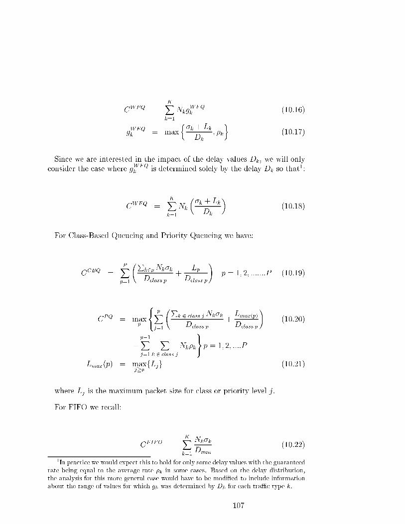
CWFQ =

KXk=1

NkgWFQk (10.16)

gWFQk = max

��k + Lk

Dk

; �k

�(10.17)

Since we are interested in the impact of the delay values Dk, we will only

consider the case where gWFQk is determined solely by the delay Dk so that

1:

CWFQ =

KXk=1

Nk

��k + Lk

Dk

�(10.18)

For Class-Based Queueing and Priority Queueing we have:

CCBQ =

PXp=1

Pk2pNk�k

Dclass p

+Lp

Dclass p

!p = 1; 2; :::::::P (10.19)

CPQ = max

p

8<:

pXj=1

Pk 2 class j Nk�k

Dclass p

+Lmax(p)

Dclass p

!(10.20)

+p�1Xj=1

Xk 2 class j

Nk�k

9=; p = 1; 2; ::::P

Lmax(p) = maxj�p

fLjg (10.21)

where Lj is the maximum packet size for class or priority level j.

For FIFO we recall:

CFIFO =

KXk=1

Nk�k

Dmin

(10.22)

1In practice we would expect this to hold for only some delay values with the guaranteed

rate being equal to the average rate �k in some cases. Based on the delay distribution,

the analysis for this more general case would have to be modi�ed to include information

about the range of values for which gk was determined by Dk for each traÆc type k.

107

where Dmin = minkfDkg.

We assume that the delay boundsDk have known independent distributions

with means Dk. We also assume that we assess the impact of the delay

distribution of each traÆc type by sampling the distribution of interest with

all other delay values set to their mean values. Applying Equations 10.5 and

10.6 the expected value and variance of the capacity will be given by:

EfCg = C +1

2

KXk=1

@2C

@D2

k

V ar[Dk] (10.23)

V ar[C] =KXk=1

@C

@Dk

!2

V ar[Dk] (10.24)

where C is the capacity when the delay bounds are at their mean values.

Using this approach we can �nd the sensitivity indices and partial variances

for each traÆc handling scheme. Note that in the equations that follow all

partial derivatives are evaluated with reference to the mean values of the

delay bounds. For WFQ we have:

@CWFQ

@Dk

=�Nk(�k + Lk)

D2

k

(10.25)

@2CWFQ

@D2k

=2 �Nk(�k + Lk)

D3

k

(10.26)

Thus the expected value and variance of the capacity are:

EfCWFQg =Xk

Nk(�k + Lk)

Dk

+Xk

Nk(�k + Lk)

D3

k

V ar[Dk] (10.27)

V ar[CWFQ] =Xk

Nk(�k + Lk)

D2

k

!2

V ar[Dk] (10.28)

For CBQ, since we are dealing with p classes, we compute sensitivity indices

and partial variances for each class as follows:

@CCBQ

@Dclass p

= �0@Pk2class pNk�k

D2

class p

+Lp

D2

class p

1A (10.29)

108

@2CCBQ

@D2class p

= 2 �0@Pk2class pNk�k

D3

class p

+Lp

D3

class p

1A (10.30)

where Dclass p is the mean delay for class p. Thus the expected value and

variance of the capacity are:

EfCCBQg =Xp

Pk2class pNk�k

Dclass p

+Lp

Dclass p

!(10.31)

+Xp

0@Pk2class pNk�k

D3

class p

+Lp

D3

class p

1AV ar[Dclass p]

V ar[CCBQ] =Xp

0@Pk2class pNk�k

D2

class p

+Lp

D2

class p

1A2

V ar[Dclass p] (10.32)

For PQ, we also calculate the sensitivity parameters on a per-class (priority-

level) basis to yield:

@CPQ

@Dclass p

= �pX

j=1

0@Pk2class j Nk�k

D2

class p

+Lmax(p)

D2

class p

1A (10.33)

@2CPQ

@D2class p

= 2 �pX

j=1

0@Pk2class j Nk�k

D3

class p

+Lmax(p)

D3

class p

1A (10.34)

Note that the values in Equations 10.33 and 10.34 apply when the maxi-

mizing class p in Equation 6.5 is unique over all possible delay values. Thus

the expected value and variance of the capacity are:

EfCPQg = maxp

8<:

pXj=1

Pk 2 class j Nk�k

Dclass p

+Lmax(p)

Dclass p

!(10.35)

+p�1Xj=1

Xk 2 class j

Nk�k +pX

j=1

0@Pk2class j Nk�k

D3

class p

+Lmax(p)

D3

class p

1AV ar[Dclass p]

9=;

V ar[CPQ] =Xp

0@ pXj=1

Pk2class j Nk�k

D2

class p

+Lmax(p)

D2

class p

1A2

V ar[Dclass p] (10.36)

109

The case where the maximizing value of p is not the same over all delay

values requires a more detailed examination of the distribution of the delays

to determine the range of values for which each class or priority-level in u-

ences the capacity in Equation 6.5. In this case the sensitivity coeÆcients

are evaluated as before but using delay values within the range of in uence

of each class. Example 1 of Section 10.3 illustrates this.

For FIFO, there is essentially one sensitivity index since we use the mini-

mum delay bound over all traÆc types. Thus,

@CFIFO

@Dmin

= �P

kNk�k

D2

min

(10.37)

@2CFIFO

@Dmin2 =

2 �PkNk�k

D3

min

(10.38)

EfCFIFOg =

PkNk�k

Dmin

+

PkNk�k

D3

min

!V ar[Dmin] (10.39)

V ar[CFIFO] =

PkNk�k

D2

min

!2

V ar[Dmin] (10.40)

The equations obtained for estimating the mean and variance of capacity

for each scheme as well as the sensitivity indices are straightforward to apply

for WFQ. However, for the other three schemes, the applicability of the

equations will depend on the ranges and inter-relations between the delay

bounds. This is because for CBQ and PQ we need to know the minimum

delay bound within an aggregation level (class or priority level) while for

FIFO we need to know the minimum delay bound over all types. When

dealing with delay bounds that have distribution functions, the determination

of the minimum bound may not be straightforward. The simplest case to

deal with is that in which the ranges of the delay bounds are non-overlapping

so that the distribution of the minimum is easily identi�ed. For more general

cases however, an analytic solution would require the use of order statistics

[1, 26] to determine the distribution of the minimum. This may prove to be

complex when the number of distributions is more than 2. For this work we

use Monte Carlo simulations to estimate the sensitivity indices for such cases

and leave the analysis using order statistics for future work.

110

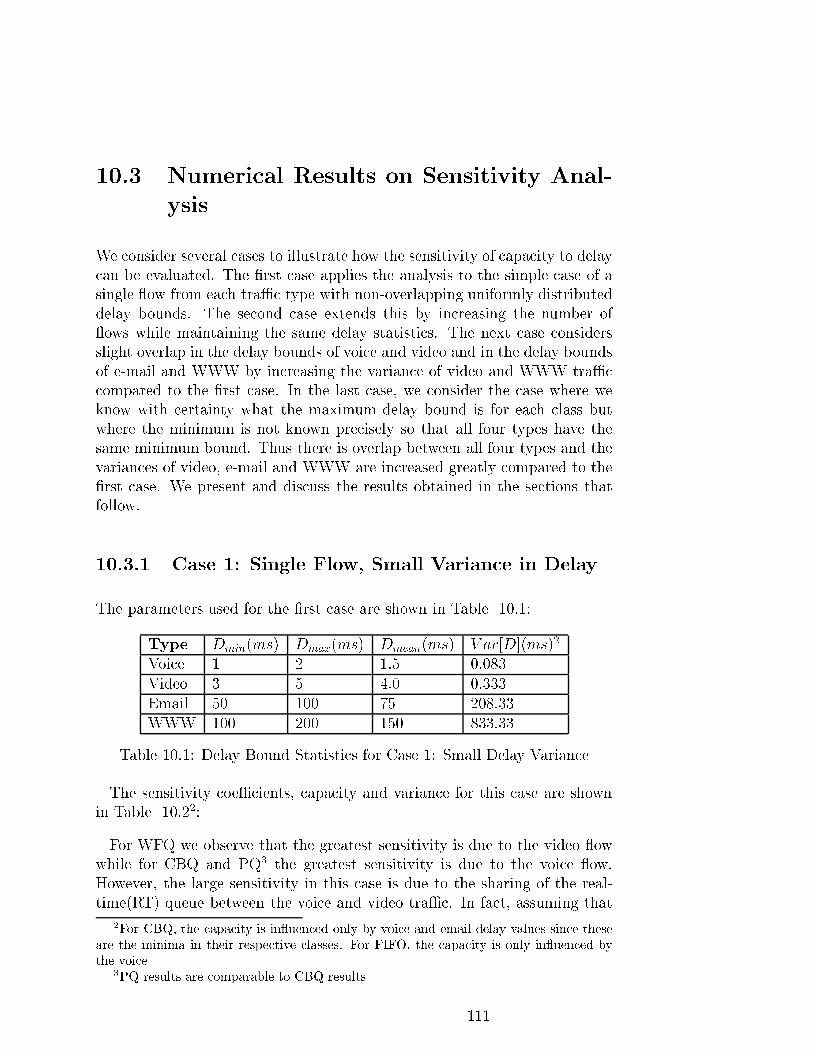
10.3 Numerical Results on Sensitivity Anal-

ysis

We consider several cases to illustrate how the sensitivity of capacity to delay

can be evaluated. The �rst case applies the analysis to the simple case of a

single ow from each traÆc type with non-overlapping uniformly distributed

delay bounds. The second case extends this by increasing the number of

ows while maintaining the same delay statistics. The next case considers

slight overlap in the delay bounds of voice and video and in the delay bounds

of e-mail and WWW by increasing the variance of video and WWW traÆc

compared to the �rst case. In the last case, we consider the case where we

know with certainty what the maximum delay bound is for each class but

where the minimum is not known precisely so that all four types have the

same minimum bound. Thus there is overlap between all four types and the

variances of video, e-mail and WWW are increased greatly compared to the

�rst case. We present and discuss the results obtained in the sections that

follow.

10.3.1 Case 1: Single Flow, Small Variance in Delay

The parameters used for the �rst case are shown in Table 10.1:

Type Dmin(ms) Dmax(ms) Dmean(ms) V ar[D](ms)2

Voice 1 2 1.5 0.083

Video 3 5 4.0 0.333

Email 50 100 75 208.33

WWW 100 200 150 833.33

Table 10.1: Delay Bound Statistics for Case 1: Small Delay Variance

The sensitivity coeÆcients, capacity and variance for this case are shown

in Table 10.22:

For WFQ we observe that the greatest sensitivity is due to the video ow

while for CBQ and PQ3 the greatest sensitivity is due to the voice ow.

However, the large sensitivity in this case is due to the sharing of the real-

time(RT) queue between the voice and video traÆc. In fact, assuming that

2For CBQ, the capacity is in uenced only by voice and email delay values since these

are the minima in their respective classes. For FIFO, the capacity is only in uenced by

the voice3PQ results are comparable to CBQ results

111

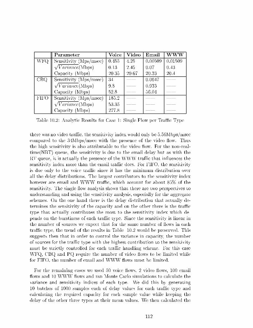
Parameter Voice Video Email WWW

WFQ Sensitivity (Mps/msec) 0.455 4.25 0.00509 0.01509pV ariance(Mbps) 0.13 2.45 0.07 0.43

Capacity (Mbps) 20.35 20.67 20.33 20.4

CBQ Sensitivity (Mps/msec) 34 | 0.0647 |pV ariance(Mbps) 9.8 | 0.933 |

Capacity (Mbps) 52.8 | 56.04 |

FIFO Sensitivity (Mps/msec) 185.2 | | |pV ariance(Mbps) 53.35 | | |

Capacity (Mbps) 277.8 | | |

Table 10.2: Analytic Results for Case 1: Single Flow per TraÆc Type

there was no video traÆc, the sensitivity index would only be 5.56Mbps/msec

compared to the 34Mbps/msec with the presence of the video ow. Thus

the high sensitivity is also attributable to the video ow. For the non-real-

time(NRT) queue, the sensitivity is due to the email delay but as with the

RT queue, it is actually the presence of the WWW traÆc that in uences the

sensitivity index more than the email traÆc does. For FIFO, the sensitivity

is due only to the voice traÆc since it has the minimum distribution over

all the delay distributions. The largest contributors to the sensitivity index

however are email and WWW traÆc, which account for about 85% of the

sensitivity. The single ow analysis shows that there are two perspectives to

understanding and using the sensitivity analysis, especially for the aggregate

schemes. On the one hand there is the delay distribution that actually de-

termines the sensitivity of the capacity and on the other there is the traÆc

type that actually contributes the most to the sensitivity index which de-

pends on the burstiness of each traÆc type. Since the sensitivity is linear in

the number of sources we expect that for the same number of ows in each

traÆc type, the trend of the results in Table 10.2 would be preserved. This

suggests then that in order to control the variance in capacity, the number

of sources for the traÆc type with the highest contribution to the sensitivity

must be strictly controlled for each traÆc handling scheme. For this case

WFQ, CBQ and PQ require the number of video ows to be limited while

for FIFO, the number of email and WWW ows must be limited.

For the remaining cases we used 50 voice ows, 2 video ows, 100 email

ows and 10 WWW ows and ran Monte Carlo simulations to calculate the

variance and sensitivity indices of each type. We did this by generating

10 batches of 1000 samples each of delay values for each traÆc type and

calculating the required capacity for each sample value while keeping the

delay of the other three types at their mean values. We then calculated the

112

variance and sensitivity index for each batch and averaged these over all the

batches.

10.3.2 Case 2: Multiple Flows, Small Variance in De-

lay

For this case we use the same delay statistics as in Table 10.1. The results

obtained analytically and from simulation will be discussed separately for

each traÆc handling scheme. The results for WFQ are shown in Table 10.3:

Parameter Voice Video Email WWW

Analytic Sensitivity (Mbps/msec) 22.7 8.5 0.509 0.151

Capacity (Mbps) 130.31 129.75 130.47 129.9pV ariance(Mbps) 6.5 4.9 7.4 4.4

% Variance 31 17 39 14

Simulation Sensitivity (Mbps/msec) 24.5 8.89 0.55 0.163

Capacity (Mbps) 130.38 129.82 130.39 129.8pV ariance(Mbps) 7.1 5.15 7.97 4.7

% Variance 31.2 16.2 38.9 13.7

Table 10.3: WFQ Analytic and Simulation Results for Case 2: Multiple

Flows, small variance

The results show a good match between the analytic and simulation re-

sults. A look at scatter plots of capacity and delay for video and WWW

in Figure 10.1 shows that for the delay statistics chosen, the capacity is an

approximately linear function of delay hence the good correlation between

the analytic and simulation results. Similar plots are obtained for voice and

email. We will observe that this correlation does not hold when we use

di�erent delay statistics for the other cases.

Looking at the sensitivity indices the capacity is most sensitive to voice

traÆc followed by video then e-mail and WWW. We �nd however that e-

mail contributes slightly more to the variance in capacity than voice. The

variance due to video is comparable to that of WWW.

For CBQ the analytic and simulation results are shown in Table 10.4.

For the analytic results we present results in terms of the RT and NRT

traÆc classes while for the simulation results we are able to consider the

impact of each traÆc type separately. For this particular example since

there is no overlap between the voice and video traÆc we could replace RT

113

3 3.2 3.4 3.6 3.8 4 4.2 4.4 4.6 4.8 5122

124

126

128

130

132

134

136

138

140

142

Link

Cap

acity

(M

bps)

Video Delay (msec)

WFQ Bandwidth as a function of Video Delay

100 110 120 130 140 150 160 170 180 190 200122

124

126

128

130

132

134

136

138

140

142

Link

Cap

acity

(M

bps)

WWW Delay (msec)

WFQ Bandwidth as a function of WWW Delay

Figure 10.1: WFQ Capacity vs Delay for Video and WWW traÆc for Case

2: small delay variance

Analytic Simulation

Parameter RT NRT Voice Video Email WWW

Sensitivity (Mbps/msec) 73.6 1.02 79.4 | 1.09 |

Capacity (Mbps) 185.72 184.59 191.3 187 189.7 187pV ariance(Mbps) 21.2 14.7 23.0 | 16 |

% Variance 67.3 32.7 67.4 | 32.6 |

Table 10.4: CBQ Analytic and Simulation Results for Case 2:Multiple Flows,

small variance

114

by voice and similarly we could replace NRT by E-mail. Since the behavior

of the RT queue is determined solely by the voice traÆc we expect in the

simulation results to obtain zero contribution to the variance from the video

traÆc. The same is true of the NRT queue which is in uenced by E-mail so

that the contribution to the variance fromWWW is zero. We again observe a

good match between the analytic and simulation results. The analysis shows

that 67.3% of the uncertainty in variance is due to the Real-Time class and

since the voice delays are the minimum in this class, this is all attributable

to voice traÆc which the simulations clearly validate. The same is true for

the NRT class where e-mail is the controlling traÆc type.

For PQ we observe that when dealing with the RT queue, the results are

identical to those of CBQ but for the NRT traÆc we are faced with the

situation in which the capacity is in some cases in uenced by the RT traÆc

and in others by the NRT traÆc. Equating the capacity values due to each

class in Equation 6.5 we �nd that for delay values of NRT traÆc in the

range 50-56.62ms, the capacity is determined by the NRT class whereas for

all other values, the delay is determined by the RT class. The scatter plot in

Figure 10.2 taken from the simulations con�rms this.

50 55 60 65 70 75 80 85 90 95 100110

115

120

125

Link

Cap

acity

(M

bps)

Email Delay (msec)

PQ Bandwidth as a function of Email Delay

Figure 10.2: PQ Capacity vs Email Delay for Case 2: small delay variance

We see from Figure 10.2 that for delays less than about 57ms, the capacity

is a linear function of the email delay whereas for values above this, the

capacity does not depend on the email delay. Proceeding with the analysis

we obtain the results in Table 10.5.

The results show that voice is the most signi�cant factor in uencing the

uncertainty in the variance as well as the sensitivity of the capacity. As

expected video and WWW do not contribute to the variance in capacity since

115

Analytic Simulation

Parameter RT NRT Voice Video Email WWW

Sensitivity (Mbps/msec) 73.6 0.209 78.9 | 0.117 |

Capacity (Mbps) 114 114 114.73 110.4 111.24 110.4pV ariance(Mbps) 21.2 3.01 23.02 | 2.6 |

% Variance 98.02 1.98 98.7 | 1.3 |

Table 10.5: PQ Analytic Results for Case 2: Multiple Flows, small variance

voice and e-mail have the minimum delay values in each class respectively.

The analytic and simulation results for FIFO are shown in Table 10.6.

Analytic Simulation

Parameter Voice Voice Video Email WWW

Sensitivity (Mbps/msec) 2600 2820.2 | | |

Capacity (Mbps) 4.07e3 4.077e3 3.92e3 3.92e3 3.92e3pV ariance(Mbps) 753.6 821 | | |

% Variance 100 100 | | |

Table 10.6: FIFO Analytic and Simulation Results for Case 2: Multiple

Flows, small variance

Again as expected, both the analysis and simulation show that voice is the

only signi�cant factor since all the minimum delay values are due to the voice

traÆc.

Looking at all four schemes we �nd that for this case voice delay contributes

the most to the sensitivity of the capacity and is also a signi�cant contributor

to the variance in capacity. The �rst two cases have demonstrated that

considerable insight into the sensitivity of capacity to delay and uncertainty

in the delay variance can be obtained by applying the methodology of Section

10.2. We will consider two more cases that show results when there is more

interaction between the traÆc classes in terms of their e�ects on the capacity

as well as how the analysis performs in the face of nonlinearity.

10.3.3 Case 3: Increased Video and WWW Variance

In this case, we increased the variance of video and WWW traÆc by chang-

ing their minimum delay values to coincide with those of voice and email

respectively. The parameters are shown in Table 10.7.

116

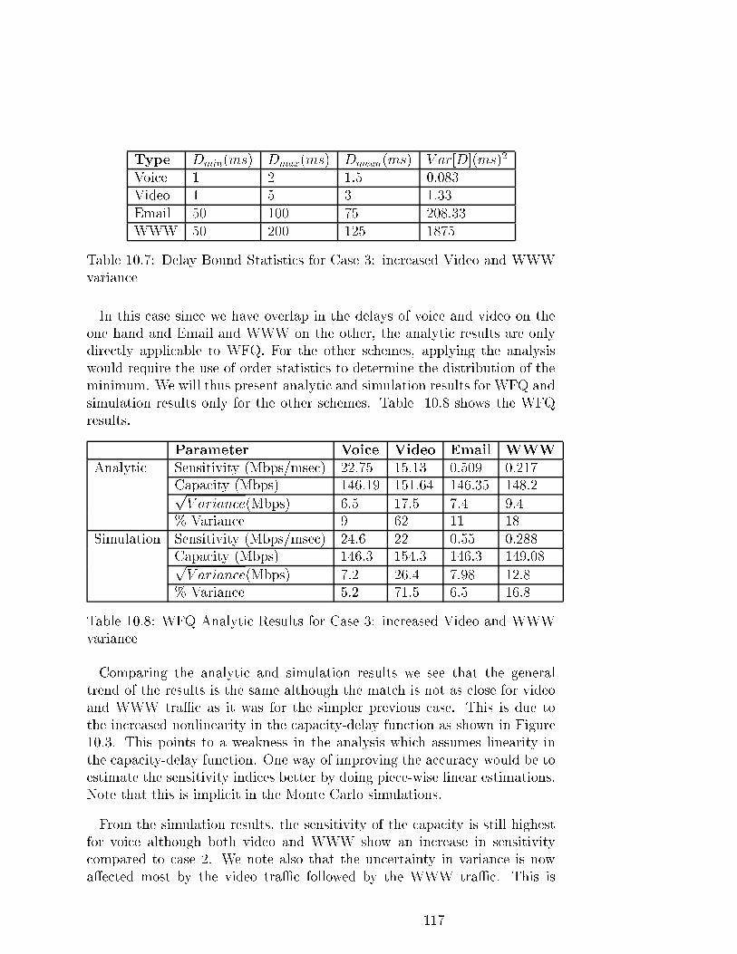
Type Dmin(ms) Dmax(ms) Dmean(ms) V ar[D](ms)2

Voice 1 2 1.5 0.083

Video 1 5 3 1.33

Email 50 100 75 208.33

WWW 50 200 125 1875

Table 10.7: Delay Bound Statistics for Case 3: increased Video and WWW

variance

In this case since we have overlap in the delays of voice and video on the

one hand and Email and WWW on the other, the analytic results are only

directly applicable to WFQ. For the other schemes, applying the analysis

would require the use of order statistics to determine the distribution of the

minimum. We will thus present analytic and simulation results for WFQ and

simulation results only for the other schemes. Table 10.8 shows the WFQ

results.

Parameter Voice Video Email WWW

Analytic Sensitivity (Mbps/msec) 22.75 15.13 0.509 0.217

Capacity (Mbps) 146.19 151.64 146.35 148.2pV ariance(Mbps) 6.5 17.5 7.4 9.4

% Variance 9 62 11 18

Simulation Sensitivity (Mbps/msec) 24.6 22 0.55 0.288

Capacity (Mbps) 146.3 154.3 146.3 149.08pV ariance(Mbps) 7.2 26.4 7.98 12.8

% Variance 5.2 71.5 6.5 16.8

Table 10.8: WFQ Analytic Results for Case 3: increased Video and WWW

variance

Comparing the analytic and simulation results we see that the general

trend of the results is the same although the match is not as close for video

and WWW traÆc as it was for the simpler previous case. This is due to

the increased nonlinearity in the capacity-delay function as shown in Figure

10.3. This points to a weakness in the analysis which assumes linearity in

the capacity-delay function. One way of improving the accuracy would be to

estimate the sensitivity indices better by doing piece-wise linear estimations.

Note that this is implicit in the Monte Carlo simulations.

From the simulation results, the sensitivity of the capacity is still highest

for voice although both video and WWW show an increase in sensitivity

compared to case 2. We note also that the uncertainty in variance is now

a�ected most by the video traÆc followed by the WWW traÆc. This is

117

1 1.5 2 2.5 3 3.5 4 4.5 5120

140

160

180

200

220

240

Link

Cap

acity

(M

bps)

Video Delay (msec)

WFQ Bandwidth as a function of Video Delay

50 100 150 200130

140

150

160

170

180

190

Link

Cap

acity

(M

bps)

WWW Delay (msec)

WFQ Bandwidth as a function of WWW Delay

Figure 10.3: WFQ Capacity vs Delay for Video and WWW traÆc for Case

3: increased Video and WWW variance

due to the increase in the delay variance of these two types. The voice and

email traÆc contribute almost equally to the uncertainty in variance. The

simulation results for CBQ are shown in Table 10.9.

Parameter Voice Video Email WWW

Sensitivity (Mbps/msec) 79.6 5.36 1.09 0.119

Capacity (Mbps) 191.45 189.95 189.87 189.72pV ariance(Mbps) 23.2 9.6 16 7.5

% Variance 57.2 9.7 27.2 5.9

Table 10.9: CBQ Simulation Results for Case 3: increased Video and WWW

variance

The sensitivity of the capacity is still highest for voice but we now have

sensitivity due to the video and WWW traÆc compared to case 2 where there

was none. Video and WWW also contribute to the variance in capacity but

voice is still the most signi�cant source of uncertainty followed by e-mail.

Note also that the net contribution due to the RT class (57.2 + 9.7) is

roughly the same as the net contribution due to the RT class in case 2. The

simulation results for PQ are shown in Table 10.10.

The voice traÆc contributes the most to the uncertainty in variance fol-

lowed by video. The email and WWW contribution is not very signi�cant.

We again note that the net contribution of the RT class to the variance is the

same as in case 2. The analytic and simulation results for FIFO are shown

in Table 10.11.

118

Parameter Voice Video Email WWW

Sensitivity (Mbps/msec) 79.2 5.36 0.119 0.0161

Capacity (Mbps) 114.89 113.33 111.24 110.67pV ariance(Mbps) 23.2 9.6 2.6 1.5

% Variance 84.2 14.4 1.0 0.4

Table 10.10: PQ Simulation Results for Case 3: increased Video and WWW

variance

Parameter Voice Video Email WWW

Sensitivity (Mbps/msec) 2830 191 | |

Capacity (Mbps) 4.08e3 4.03e3 3.92e3 3.92e3pV ariance(Mbps) 825.8 339.1 | |

% Variance 86.4 13.6 | |

Table 10.11: FIFO Simulation Results for Case 3: increased Video and

WWW variance

Voice and video are now the most signi�cant factors contributing to the

uncertainty in capacity variance with voice clearly dominating. Email and

WWW delays have no impact on the variance because the minimum delay

values come from either the voice or video distributions.

10.3.4 Case 4: Increased Email and WWW Variance

For the last case we consider the case where the uncertainty in the Email

and WWW delays is greatly increased over that of the previous case. The

delay bound statistics are shown in Table 10.12.

Type Dmin(ms) Dmax(ms) Dmean(ms) V ar[D](ms)2

Voice 1 2 1.5 0.083

Video 1 5 3.0 1.33

Email 1 100 50.5 816.75

WWW 1 200 100.5 3300.08

Table 10.12: Delay Bound Statistics for Case 4: increased Email and WWW

variance

As with the previous case where video and WWW had increased variance,

analytic results can only be provided for WFQ. Table 10.13 shows the results

for WFQ.

We observe that the analytic and simulation results show the same trend in

119

Parameter Voice Video Email WWW

Analytic Sensitivity (Mbps/msec) 22.75 15.13 1.12 0.336

% Variance 2.5 17.4 58.8 21.3

Simulation Sensitivity (Mbps/msec) 24.5 21.7 6.06 0.256pV ariance(Mbps) 7.18 26.4 248 238.8

% Variance 0.04 0.6 52 48

Table 10.13: WFQ Analytic and Simulation Results for Case 4: increased

Email and WWW variance

the ranking of the contribution of each traÆc type to the variance although

there is marked disparity in the exact numbers for video and WWW traf-

�c. With the current delay statistics the capacity-delay functions for email

and WWW are extremely nonlinear as shown in Figure 10.4. The current

0 10 20 30 40 50 60 70 80 90 1000

500

1000

1500

2000

2500

3000

Link

Cap

acity

(M

bps)

Email Delay (msec)

WFQ Bandwidth as a function of Email Delay

0 20 40 60 80 100 120 140 160 180 2000

500

1000

1500

2000

2500

3000

3500

Link

Cap

acity

(M

bps)

WWW Delay (msec)

WFQ Bandwidth as a function of WWW Delay

Figure 10.4: WFQ Capacity vs Email and WWWDelay for Case 4: increased

Email and WWW variance

analysis is not able to capture the e�ects of this nonlinearity hence the pre-

dicted sensitivity coeÆcients for Email and WWW are not accurate. This

inaccuracy in turn a�ects the variance results. However we can observe from

the simulation that Email is now the most signi�cant factor, contributing to

about 50% of the variance, followed by WWW traÆc. For CBQ, Table 10.14

shows that email and WWW are the most signi�cant factors contributing to

the variance in capacity, together accounting for almost all of the variance in

capacity.

In terms of the sensitivity however, voice is still the highest followed by

email then video and WWW. The PQ results are shown in Table 10.15. We

observe the same trends as for CBQ in the variance contribution of each traÆc

120

Parameter Voice Video Email WWW

Sensitivity (Mbps/msec) 79.3 5.13 12 3.75pV ariance(Mbps) 23.2 9.47 497.94 392.25

% Variance 0.13 0.02 61.5 38.35

Table 10.14: CBQ Simulation Results for Case 4: increased Email andWWW

variance

Parameter Voice Video Email WWW

Sensitivity (Mbps/msec) 32.7 3.04 12 3.85pV ariance(Mbps) 11.6 6.32 506.85 402.74

% Variance 0.03 | 61 38.97

Table 10.15: PQ Simulation Results for Case 4: increased Email and WWW

variance

type although the sensitivity indices are di�erent. Voice has the highest

sensitivity index followed by email, then WWW and Video. For FIFO, voice

and video are the most signi�cant factors both in terms of sensitivity and

variance in capacity as shown in Table 10.16. This is because only a small

Parameter Voice Video Email WWW

Sensitivity (Mbps/msec) 2820 182 0.679 0.184pV ariance(Mbps) 825.8 336.98 64.17 68.65

% Variance 84.8 14.1 0.5 0.6

Table 10.16: FIFO Simulation Results for Case 4: increased Email and

WWW variance

proportion of samples from the email and WWW distributions (0.5% and

0.25% respectively) are small enough to be the minimum value that determine

the capacity.

The four cases in this section have validated the methodology and analy-

sis that can be used to perform uncertainty and sensitivity analysis for the

four traÆc handling schemes. Numerical simulations can be used to per-

form the sensitivity analysis while the theoretical analysis is valid only when

the capacity-delay function is linear. More work is needed to extend and

generalize the theoretical formulation to cover all cases.

121

10.4 Summary

In this chapter we have shown how a stochastic formulation of the delay re-

quirements can be used to provide some understanding of how the capacity

required by di�erent traÆc handling schemes is a�ected by uncertainty in the

values of the maximum delay bounds. We have developed and demonstrated

a methodology for performing uncertainty and sensitivity analysis which can

be used to capture how uncertainty in delay bounds translates into uncer-

tainty in the network capacity. A purely analytic solution has been obtained

with the accuracy being largely dependent on the linearity of the capacity-

delay function. For cases where the functions are not linear, numerical Monte

Carlo simulations were used to provide accurate results. In the next chap-

ter we conclude by discussing the relevancy of our results in the context of

network planning and design.

122

Chapter 11

Conclusion

11.1 Implications of Results on Network Ar-

chitectures

We conclude by discussing the results obtained in the context of current and

proposed approaches to the use of traÆc handling for multi-service networks.

� Best-E�ort Network

The best-e�ort network uses FIFO in both the edge and core so that the

delay guarantees are uniform across all traÆc types. From our results

we �nd that to support the QoS of delay-sensitive applications such as

voice requires abundant network capacity when the voice traÆc shares

a queue with bursty traÆc such as email and WWW. When there is no

bursty traÆc then an all-FIFO network performs just as well as a non-

FIFO network. This may seem to suggest the use of separate queues

and links (in essence a separate network) for delay sensitive traÆc to

isolate it from the bursty non-delay sensitive traÆc. The appeal of the

best-e�ort network lies in its simplicity and if network capacity is not

a constraint, then it may still be the network of choice for some.

� Class-Based Network

In a class-based network, ows are grouped into distinct classes and

resources such as queues and link bandwidth are allocated to the class

as whole. TraÆc handling approaches for this type of network include

Class-Based Queueing, Priority Queueing and Class-Based Weighted

Fair Queueing among others. Our results show that using class-based

123

traÆc handling by grouping traÆc types with similar delay objectives

can meet the delay guarantees of all traÆc types with minimal band-

width. Class-based handling in the edge with best-e�ort handling in

the core requires moderate capacity while using best-e�ort in the edge

increases the bandwidth signi�cantly. The complexity of class-based

handling may range from fair to extreme depending on the exact im-

plementation.

� Flow-Based Network

In a ow-based network, each ow is allocated its own dedicated re-

sources and as such managing the network may prove to be complex

when there are numerous ows. Using ow based handling such as

WFQ requires minimal capacity and any combination of ow-based

handling and class-based handling does not increase the bandwidth

signi�cantly. Using ow-based handling with best-e�ort handling in ei-

ther the edge or core of the network requires more abundant capacity.

Figure 11.1 summarizes the capacity requirements of combinations of edge

and core traÆc handling mechanisms.

EdgeTraffic

Handling

Core Traffic Handling

Flow-based(WFQ)

Class-based(CBQ/PQ)

Best-Effort(FIFO)

Flow-based(WFQ)

Class-based(CBQ/PQ)

Best-Effort(FIFO)

KEY

Increasing Network Capacity

Figure 11.1: Capacity Requirements of Edge and Core TraÆc Handling

Mechanisms

The diagram uses di�erent shades of gray to show how the capacity re-

quirements change depending on the type of traÆc handling used in the edge

and core portions of the network. For example, we see that with ow-based

124

handling in the edge, class-based handling in the core requires comparable

capacity to ow-based handling in the core. Given that one objective is to

simplify network management, the use of ow-based handling in the core

portion of the network may not be practical and the choice between which

combination of traÆc handling mechanisms to use will depend in part on

the availability of bandwidth in the edge and core portions of the network.

With moderate amounts of bandwidth in the core, then either class-based or

ow-based handling can be used in the edge with best-e�ort handling in the

core portion of the network. If some complexity in the core can be tolerated

then with minimal capacity, ow-based or class-based handling can be used

in the edge with class-based handling in the core.

11.2 Practical Applications of Sensitivity Anal-

ysis

The methodology in Section 10.3 uses a one-at-a-time (OAT) approach by

considering how each delay distribution a�ects the capacity individually. For

practical purposes, one would like to use the analysis for the more general case

where any number of traÆc types may have stochastic delay bounds. Careful

examination of the equations for the variance of capacity in Section 10.2

shows that the total variance is simply the sum of the variance due to each

individual delay distribution. We can thus use the analysis to upper-bound

the standard deviation in capacity for di�erent distributions of the delay

parameters. Speci�cally, suppose the total variance in capacity is V ar[C] =

V ar[C1]+V ar[C2]+ :::::+V ar[Ck] where V ar[Ck] is the variance in capacity

due to the kth delay distribution. Then the standard deviation is given by:

SD(C) =qV ar[C1] + V ar[C2] + :::::::: + V ar[Ck]

<

sV ar[C1] + V ar[C2] + :::::::: + V ar[Ck] +

Xi6=j

SD(i)SD(j)

<

q(SD(1) + SD(2) + :::::::SD(k))2

< SD(1) + SD(2) + :::::::SD(k)

where SD(i) =qV ar[Ck]. Thus changes in one or more delay parameters

can easily be used to assess the e�ect on the total capacity.

125

The methodology used for the single-link analysis extends easily to edge-

core networks. The OAT approach can be applied to di�erent edge-core

architectures and sensitivity indices calculated for each link in the network.

From this information the average sensitivity in the edge and core portions

as well as variance in the edge and core capacity can be easily calculated.

With this in mind we turn now to some ways in which sensitivity analysis

can be used in network design and provisioning.

� Planning and Forecasting

Sensitivity analysis can be used to determine how changes in traÆc

patterns will impact the capacity requirements of a network. The sen-

sitivity indices can be used to determine the expected capacity and

standard deviation of capacity for di�erent traÆc conditions which can

then be used to predict at what point in time the network capacity will

need to be upgraded to support traÆc growth. It should be noted that

such planning has also been discussed in the context of deterministic

delay bounds but the value added by a stochastic formulation is the

incorporation of how uncertainty in the knowledge of the delay bounds

will impact the capacity requirements. Using the sensitivity analysis

allows the network planner to consider how the addition of new ser-

vices whose delay expectations are not known precisely may impact

the capacity requirements.

Another way to use the sensitivity analysis is to determine how chang-

ing trends in delay requirements of di�erent services will impact net-

work capacity requirements. As telecommunication networks and the

Internet evolve, di�erent applications will emerge with new delay re-

quirements. There is thus a need for a methodology that can be used to

assess how such changes will a�ect the network design and sensitivity

analysis can be used for this.

� Service Provisioning

By using the sensitivity analysis to determine how imperfect knowledge

of maximum delay requirements a�ects network capacity, a network

engineer will be in a better position to de�ne the types of services

that the network can o�er within the limits of its existing capacity

framework.

� Network Management

Sensitivity analysis can also be used to guide network users on suitable

traÆc parameters for the type of service they desire. For instance if a

user is aware of the rate and burstiness parameters, then the analysis

126

can be used to de�ne an appropriate range of delay objectives for a

given capacity or can be used to determine the capacity requirements

needed to satisfy speci�c delay objectives.

11.3 Summary of Contributions

There are four main contributions made by this thesis:

� The most signi�cant contribution is in developing a methodology that

can be used to quantify and compare the capacity requirements of dif-

ferent traÆc handling approaches. There has always been a general

consensus that larger amounts of capacity are required by FIFO traÆc

handling compared to per- ow handling without speci�cs on how to

quantify the di�erence. There have also been notions about the capac-

ity requirements of class-based handling being intermediate between

per- ow and FIFO but also with no quanti�cation. Through the work

we have done we have established an analytic methodology that has

quanti�ed the di�erences in capacity and that can be used to address a

variety of questions relating to design of integrated services networks.

� We began this thesis with the objective of answering the question of

how di�erent traÆc management approaches compare in terms of their

capacity requirements. We have shown that class-based schemes do not

di�er signi�cantly from ow-based schemes in their capacity require-

ments which was one of the issues surrounding the Integrated Services

vs Di�erentiated services debate of the last couple of years. We have

also shown that there are a number of issues that must be factored in

when comparing traÆc handling schemes such as the aggregate bursti-

ness, the network size and the connectivity of the network.

� The work on sensitivity analysis provides a �rst-step in the development

of procedures for long-term network planning. By incorporating other

parameters such as burstiness, topology and traÆc composition into the

sensitivity analysis valuable insight can be obtained for use in network

design and planning.

� Lastly, we have extended the application of Network Calculus in ad-

dressing a signi�cant networking problem.

127

11.4 Future Work

We have identi�ed several areas for future work:

� In this work we used a deterministic model to characterize the applica-

tion traÆc. This assume worst-case behavior on the part of the sources

generating the traÆc and is thus a conservative approach. An exten-

sion to this work would thus look at the use of stochastically bounded

traÆc models _Some work has been done with stochastically bounded

models such as the work in [14, 51, 66, 79, 92].

� Another area for future work is in obtaining better bounds on utiliza-

tion for networks that use aggregate traÆc handling. We reported in

Chapter 9 on the work in [17] which provides very pessimistic results

on allowable utilization. One issue not considered here is a detailed

study on utilization and network topology to determine how our re-

sults compared to the bounds in [17].

� In Chapter 8 we developed some analytic results for bounds on capacity

requirements in edge-core networks but we did not test the accuracy of

the bounds exhaustively. Future work would look at how good these

bounds are by conducting analyses on networks of varying topology as

was done here. This would provide results and insight into e�ective

uses of the bounds.

� There are several items related to the sensitivity analysis that are left

open for future work. The �rst is obtaining an analytic solution using

order statistics to deal with the general cases in which the minimum

delay distribution is not easily identi�ed. In view of the fact that the

complexity of using order statistics may not justify the e�ort, Monte

Carlo simulations as used here, may still prove to be the best solution.

The second item has to do with the use of global sensitivity analysis

such as the importance measures described in Section 10.1. A complete

uncertainty and sensitivity analysis should incorporate elements of both

local and global analysis and we emphasized local analysis in this work.

It would complete the work to consider further insight that may be

obtained from global analysis.

128

Bibliography

[1] Arnold B., N. Balakrishnan, H. Nagaraja, A FirstCourse in Order Statistics, J. Wiley and Sons, 1993.

[2] Atherton R.W., R.B. Schainker, E.R. Ducot, On the

Statistical Sensitivity Analysis of Models for Chem-

ical Kinetics, AICheJ. 21, p.441-448, 1975.

[3] ATM Forum, Draft TM 4.1 TraÆc Management

Speci�cation, Dec 1998.

[4] Bajaj S., L. Breslau, S. Shenker, Is Service Priority

Useful in Networks?, Proc. ACM SIGCOMM 1998,

p66-77.

[5] Bernet Y., Integrating RSVP and Di�serv, Internet

Bandwidth Summit, iBAND2, May 1999.

[6] Black D., Building Switched Networks, Addison-

Wesley-Longman Inc.,1999.

[7] Blake S. et al., A Framework for Di�erentiatedServices, IETF Internet Draft, draft-ietf-di�serv-

framework-02, Feb. 1999.

[8] Blake S. et al., An Architecture for Di�erentiated

Services, IETF Internet Draft, draft-ietf-di�serv-

arch-02, Oct. 1998.

[9] Braden R., D. Clark, S. Shenker, Integrated Services

in the Internet Architecture: an Overview IETF

RFC 1633, June 1994.

[10] Braden R. et al, Resource Reservation Protocol

(RSVP) - v1. Functional speci�cation, IETF RFC

2205, Sept. 1997.

129

[11] Bragg A., Wright S., Delay Bounds for a mix of

Latency-Rate(LR) and non-LR Schedulers, ATM

Forum Contribution, 99-0595, December 1999.

[12] Breslau L., S. Shenker, Best E�ort versus Reserva-

tions: A Simple Comparative Analyis, Proc. ACM

SIGOCMM 1998, p.3-16.

[13] Burakowski W., Performance of Premium Service

in IP QoS Networks, Proc. 7th Intl. Conf. on Ad-

vanced Computer Systems, Poland, Oct. 2000.

[14] Chang C.S., Stability, Queue Length and Delay of

Deterministic and Stochastic Queueing Networks,IEEE Trans. on Automatic Control, vol 39, no. 5,

May 1994.

[15] Chang C.S., Performance Guarantees in Communi-

cation Networks, Springer-Verlag, 2000.

[16] Charny A.,Delay Bounds in a Network withAggregate Scheduling, ftp:ftpeng.cisco.com/ftp/

acharny/aggregate delay v4.ps, Feb. 2000

[17] Charny A., J. Leboudec, Delay Bounds in a Networkwith Aggregate Scheduling, 1st International Work-

shop on Quality of future Internet Services, QofIS

2000, Sept. 2000.

[18] Chiussi F, A. Francini, Implementing Fair-Queueingin ATM Switches - Part 1: A Practical Methodology

for the Analysis of Delay Bounds, IEEE 1997.

[19] Cisco Government A�airs Website, Facts and Statis-

tics,www.cisco.com/warp/public/779/govta�s/factsNStats/internetusage.html.

[20] Clark D., W. Fang, Explicit Allocation of Best Ef-fort Packet Delivery Service, IEEE/ACM Trans. on

Networking, vol.6, no.4, Aug. 1998.

[21] Clark D., S.Shenker, L Zhang, Supporting Real-timeApplications in an integrated Services Packet Net-

work: Architecture and Mechanisms, Proc. ACM

SIGCOMM 1992, p. 14-26.

130

[22] Class Data Systems, Providing Enterprise Wide

End-to-End QoS www.classdata.com/whiteP-

no1.html.

[23] Cruz R.L., A Calculus for Network Delay, Part I:

Network Elements in Isolation, IEEE Transactions

on Information Theory, Vol 37, no. 1, Jan, 1991.

[24] Cruz R.L., A Calculus for Network Delay, Part II

: Network Analysis, IEEE Transactions on Informa-

tion Theory, Vol 37, no. 1, Jan, 1991.

[25] Cruz R.L., Quality of Service Guarantees in Virtual

Switched Networks, IEEE JSAC, vol 13, no. 6, Aug.

1995.

[26] David H.A., Order Statistics, 2nd ed., J. Wiley and

Sons, 1981.

[27] Demers A., S. Keshav, S. Shenker, Analysis and

Simulation of a Fair Queueing Algorithm, Proc.

ACM SIGCOMM 1989, p.1-11.

[28] de Veciana G., G. Kesidis, Bandwidth Allocation forMultiple Qualities of Service using Generalized Pro-cessor Sharing, IEEE Trans. on Information Theory,

vol. 42, no.1 1996.

[29] Dolzer K.,W. Payer, M. Eberspacher, \A Simula-

tion Study of TraÆc Aggregation in Multi-ServiceNetworks", Proc. IEEE Conference on High Per-

formance Switching and Routing, Heidelberg, June

2000.

[30] Dovrolis C.,A Case for Relative Di�erentiated Ser-

vices and the Proportional Di�erentiation Model,

IEEE NW, Sept/Oct. 1999.

[31] Eichler G. et al, Implementing Integrated and Dif-

ferentiated Services for the Internet with ATM Net-works: A Practical Approach, IEEE COM. Jan

2000, p132

[32] Elwalid A., d. Mitra, R. Wentworth, A New Ap-proach for Allocating Bu�ers and Bandwidth to

131

Heterogeneous Regulated TraÆc in an ATM Node,

IEEE/ACM Trans. on Networking, v.13, no. 6, Aug.

1995, p1165-1127.

[33] Elwalid A., D. Mitra, Design of Generalized Proces-

sor Sharing Schedulers which Statistically Multiplex

Heterogeneous QoS Classes, Proc. IEEE Infocom,

April 1999.

[34] Ferguson P.,G. Huston, Quality of Service, deliver-

ing QoS on the Internet and in Corporate Networks,

J. Wiley & Sons Inc, 1998.

[35] Ferrari D., Client Requirements for Real-time Com-munication Services, IEEE Communications Maga-

zine Nov. 1990 p. 65-72.

[36] Fiedler U., P. Huang, B. Plather, Over-provisioning or Di�erentiated Services - ACase Study on Integrating Services over IP,

www.tik.ee.ethz.ch/ �edler/papers/provisioning.pdf.

[37] Fischer S., Cooperative QoS Management for Multi-media Applications Proc. International Conference

on Multimedia Computing and Systems, 1997.

[38] Floyd S., V. Jacobson, Link-sharing and Re-source Management Models for Packet Networks,

IEEE/ACM Trans. On Networking, vol 3, no, 4,

Aug. 1995.

[39] Georgiadis L., R. Guerin, V. Peris, R. Rajan, EÆ-

cient Support of Delay and Rate Guarantees in an

Internet, Proc. ACM SIGCOMM 1996, p.106-116.

[40] Goyal P., S. Lam, H. Vin, Determining end-to-endDelay Bounds in Heterogeneous Networks, Multime-

dia systems vol. 5, no. 3, May 1997, p.157-163.

[41] Guerin R., S. Kamat, V. Peris, R. Rajan, Scalable

QoS Provision through Bu�er Management, Proc.

IEEE Infocom 1999.

[42] Guerin R., V. Peris, Quality of Service in PacketNetworks: Basic Mechanisms and Directions, Com-

puter Networks, vol 31, 1999.

132

[43] Hayes D., M. Rumsewicz, L. Andrew, Quality of

Service Driven Packet Scheduling Disciplines for

Real-Time Applications: looking beyond fairness,

Proc. IEEE Infocom 1999

[44] Holliday C., We have found the killer ap-

plication and it's killing us, Internet Tele-

phony, www.internettelephony.com/archive /fea-

turearchive/7.20.98.html, 1998.

[45] IETF RFC 2211, Speci�cation of the Controlled-Load Network Element Service,ftp://ftp.isi.edu/in-

notes/rfc2211.txt.

[46] IETF RFC 2212, Speci�cation of Guaranteed Qual-

ity of Service,ftp://ftp.isi.edu/in-notes/rfc2212.txt.

[47] Iida K., Performance Evaluation of the Architecture

for End-to-End QoS Provisioning, IEEE COM, vol.

38, no. 4, April 2000.

[48] Isenberg D.S., The Dawn of the Stupid Network,

www.isen.com/papers/Dawnstupid.html

[49] Kilkki K., Di�erentiated Services for the Internet,Macmillan Technical Publishing, 1999.

[50] Kim H., W. Leland, S. Thomson, Evalu-ation of Bandwidth Assurance Service us-

ing RED for Internet Service Di�erentia-tion,ftp://ftp.bellcore.com/pub/world/hkim/assured.ps.Z

[51] Knightly E. , H. Zhang, TraÆc Characterization

and Switch Utilization using a Deterministic Bound-

ing Interval Dependent TraÆc Model, Proc. IEE In-

focom, 1995,p. 1137-1145..

[52] Le Boudec J., Network Calculus MadeEasy, Tech. Report EPFL-DI 96/218,

http://lrcwww.ep .ch/PS�les/d4paper.ps, Dec.

1996.

[53] Le Boudec J, Application of Network Calculus to

Guaranteed Service Networks, IEEE Trans. on In-

formation Theory, vol. 44, no. 3, May 1998.

133

[54] Le Boudec J., G. Hebuterne, Comment on "A De-

terministic Approach to the End-to-End Analysis

of Packet Flows in Connection-Oriented Networks",

IEEE/ACM Trans. on Networking, vol. 8, no. 1,

Feb. 2000.

[55] Le Boudec J., P. Thiran, A Short Tutorial on Net-

work Calculus I: Fundamental Bounds in Commu-

nication Networks, Proc. ISCAS 2000, Geneva, May

2000.

[56] Le Boudec J., P. Thiran, Network Calculus: A The-

ory of Deterministic Queueing Systems for the In-ternet, Springer-Verlag 2001.

[57] Liebeherr J., S. Patek, E. Yilmaz, Tradeo�s in De-signing Networks with End-to-End Statistical QoSGuarantees, Proc. IEEE/IFIP 8th Intl. Workshop

on QoS, IWQoS 2000, Philadelphia, June 2000.

[58] Mark B., G. Ramamurthy, Real-Time TraÆc Char-

acterization for Quality-of-Service Control in ATMNetworks, IEICE Trans. Comm. vE81-B, no. 5, May

1998.

[59] McKay M.D., Evaluating Prediction Uncertainty,

Technical Report NUREG/CR-6311, US Nuclear

Regulatory Commission, 1995.

[60] Microsoft, Quality of Service Technical White Pa-per,www.microsoft.com/windows2000/techinfo/howitworks/

communications/traÆcmgmt/qosover.asp, Sept.

1999.

[61] Naser H., A. Leon-Garcia, O.Aboul-Magd, Voice

over Di�erentiated Services, IETF Draft, draft-

naser-voice-di�serv-eval-00, Dec. 1998.

[62] Parekh A., R. Gallager, A Generalized Processor

Sharing Approach to Flow Control in Integrated Ser-vices Networks: The Single Node Case, IEEE/ACM

Transactions on Networking, Vol. 1, no. 3, June

1993.

134

[63] Parekh A., R. Gallager, A Generalized Proces-

sor Sharing Approach to Flow Control in Inte-

grated Services Networks: The Multiple Node Case,

IEEE/ACM Transactions on Networking, Vol. 2,

no. 2, April 1994.

[64] Presti F.L., Z. Zhang, D. Towsley, Bounds, Approxi-

mations and Application for a Two-Queue GPS Sys-

tem Proc. IEEE Infocom 1996, p.1310-1317.

[65] Presti F., Z. Zhang, J. Kurose, Source Time-Scaleand Optimal Bu�er/Bandwidth Tradeo� for Het-

erogeneous Regulated TraÆc in a Network Node,IEEE/ACM Trans. on Networking, vol. 7, no. 4,

Aug. 1999.

[66] Qiu J., E. Knightly, Inter-Class Resource Sharingusing Statistical Service Envelopes, Proc. IEEE In-

focom, 1999.

[67] Reisslein M., K. Ross, S. Rajagopal, Guaranteeing

Statistical QoS to Regulated TraÆc: the Single NodeCase, IEEE Infocom 1999.

[68] Reisslein M., K. Ross, S. Rajagopal, Guaranteeing

Statistical QoS to Regulated TraÆc: the Multiple

Node Case, Proc. IEEE Conference on Decision and

Control, 1998, p531-538.

[69] Sahni J., P. Goyal, H. Vin, Scheduling CBR Flows:

FIFO or Per-Flow Queueing.

[70] Sahu S., D. Towsley, J. Kurose, A Quantitative

Study of Di�erentiated Services for the Internet,Umass CMPSCI Tech Report 99-09, University of

Massachusetts, 1999.

[71] Saltelli A.,K. Chan, E.M. Scott, ed. Sensitivity

Analysis, J. Wiley and Sons, 2000.

[72] Sariowan H., R. Cruz, G. Polyzos, Scheduling for

Quality of Service Gurantees via Service Curves,

Proc, ICC, 1995.

135

[73] Schmitt J.,Aggregation of Guaranteed Service Flows

TR-KOM-1998-06, http://www.kom.e-technik.tu-

darmstadt.de

[74] Schwartz M., Broadband Integrated Networks, Pren-

tice Hall, 1996.

[75] Seddigh N., B. Nandy, P. Pieda, Bandwidth Assur-ance Issues for TCP ows in Di�erentiated Services

Network, Proc. IEEE Globecom 1999.

[76] Shenker S., Fundamental Design Issues for the Fu-

ture Internet, IEEE JSAC vol.13, no. 7, Sept. 1995.

[77] Stardust Forums, Internet Bandwidth ManagementWhitepaper, Proc. Internet Bandwidth Summit,

iBAND2, May 1999.

[78] Stardust Forums, The Need for Quality of Service,

www.stardust.com/qos/whitepapers/need.html,

July 1999

[79] Starobinski D., M. Sidi, Stochastically Bounded

Burstiness for Communication Networks, IEEE In-

focom 1999.

[80] Stilliadis D., A. Varama, Latency-Rate Servers: AGeneral Model for Analysis of TraÆc Scheduling Al-

gorithms, IEEE/ACM Trans. on Networking vol. 6,

no. 5, Oct. 1998, p.611-624.

[81] Stoica I., S. Shenker, H. Zhang, Core-Stateless Fair

Queueing: Achieving Approximately Fair Band-

width Allocations in High Speed Networks, Proc.

ACM SIGCOM, p118-130, Vancouver, 1998.

[82] Stoica I., H. Zhang, Providing Guaranteed ServicesWithout Per-Flow Management, Proc. ACM SIG-

COMM 1999, p.81-95.

[83] Tanenbaum A.S., Computer Networks 3rd ed., Pren-

tice Hall 1996, p348-352

[84] Tatipamula M., B. Khasnabish, Multimedia Com-munication Networks: Techniques and Services,

Artech House 1998.

136

[85] Trecordi V., G. Verticale, QoS Support for per- ow

services: Packet over SONET vs IP over ATM,

IEEE Internet Computing, July/Aug 2000 p.58

[86] Van der Wal K., M. Mandjes, H. Bastiaangen, Delay

Performance Analysis of the New Internet Services

with Guaranteed QoS, Proc. IEEE, v85 no.12, Dec.

1997

[87] Verma P., A. Rybczynski, The Economics of Seg-

regated and Integrated Systems in Data Commu-

nication with Geometrically Distributed MessageLengths, IEEE Trans. on Comm. Nov. 1974, p.1844-

1848.

[88] Wexler J., The QoS Conundrum, Business Commu-nication Review, April 2001, p.48

[89] Wrege D., E. Knightly, H. Zhang, J. Liebeherr, De-terministic Delay Bounds for VBR Video in Packet-

Switching Networks: Fundamental Limits and Prac-

tical Tradeo�s, IEEE/ACM Trans. On Networking,

vol 4, no.3, June 1998.

[90] Wright S., Delay Accumulation Procedures, ATMForum Contribution, 99-0149, April 1999.

[91] Wright S., Delay Accumulation Proposal, ATM Fo-

rum Contribution, 99-0295, July 1999.

[92] Yaron O., M Sidi, Performance and Stability of

Communication Networks via Robust Exponential

Bounds, IEEE/ACM Trans. On Networking, vol.1,

no. 3, June 1993, p372-385.

[93] Zhang H.,S. Keshav, Comparison of Rate-BasedService Disciplines, Proc. ACM SIGCOMM 1991,

p.113-121.

[94] Zhang, H. D. Ferrari, Rate-Controlled Static Prior-

ity Queueing, Proc. IEEE INFOCOM 1993, p. 227-

236.

[95] Zhang H., Service Disciplines for Guranteed Perfor-mance Service in Packet Switching Networks, Proc.

IEEE, vol. 83, no. 10, Oct. 1995.

137

[96] Zhang Z., D. Towsley, J. Kurose, Statistical Analy-

sis of the Generalized Processor Sharing Scheduling

Discpline, IEEE JSAC, vol. 16, no. 6, Aug. 1995

[97] Zhang Z., Z. Duan, Y. Hou, Fundamen-

tal Tradeo�s in Aggregate Packet Schedul-

ing, www.cs.umin.edu/Research/CNMRG/ Pa-

pers/Zhan01/Fundamental TR.pdf, Jan 2001.

138