t.r. gebze technical university graduate school of

T.R.

GEBZE TECHNICAL UNIVERSITY

GRADUATE SCHOOL OF NANOTECHNOLOGY

FABRICATION AND CHARACTERIZATION OF

MINIATURIZED FLUXGATE SENSORS

FATMANUR KOCAMAN

A THESIS SUBMITTED FOR THE DEGREE OF

MASTER OF SCIENCE

NANOSCIENCE AND NANOENGINEERING

GEBZE

2019

T.R.

GEBZE TECHNICAL UNIVERSITY

GRADUATE SCHOOL OF NANOTECHNOLOGY

FABRICATION AND

CHARACTERIZATION OF MINIATURIZED

FLUXGATE SENSORS

FATMANUR KOCAMAN

A THESIS SUBMITTED FOR THE DEGREE OF

MASTER OF SCIENCE

NANOSCIENCE AND NANOENGINEERING

THESIS SUPERVISOR

PROF. DR. MUHAMMED HASAN ASLAN

II. THESIS SUPERVISOR

ASSIST. PROF. DR. TURGUT TUT

GEBZE

2019

T.C.

GEBZE TEKNİK ÜNİVERSİTESİ

NANOTEKNOLOJİ ENSTİTÜSÜ

MİNYATÜRİZE EDİLMİŞ FLUXGATE

SENSÖRLERİN FABRİKASYONU VE

KARAKTERİZASYONU

FATMANUR KOCAMAN

YÜKSEK LİSANS TEZİ

NANOBİLİM VE NANOMÜHENDİSLİK

ANABİLİM DALI

DANIŞMANI

PROF. DR. MUHAMMED HASAN ASLAN

II. DANIŞMANI

DR. ÖĞR. ÜYESİ TURGUT TUT

GEBZE

2019

v

SUMMARY

Magnetic sensors have been the devices in which have been greatly worked for

many years. Fluxgate sensors are more suitable and efficient than most of the other

magnetic sensors, although various magnetic field measurement device and techniques

have been used. These sensors have the advantages of high sensitivity, high

temperature stability and high reliability, and they are used to measure the magnitude

and direction of DC and low frequency AC magnetic fields. Fluxgate sensors can be

used in many applications such as location determination in satellites, magnetic track

detection, submarine mine detection and object recognation. In recent years, it has

been observed that studies on miniaturization of fluxgate sensor have increased with

the necessity of reducing the cost of the sensor and reducing the power consumption.

In this thesis study, the production of the fluxgate sensor in miniature dimensions with

orthogonal structure was realized. Cobalt-based amorphous alloy, which is frequently

preferred due to its soft material as a sensor core, was used. This amorphous alloy

which was taken as a ribbon was given a meander shape using photolithography and

chemical etching techniques. Firstly the sensor with this core was produced and

sensitivity and noise measurements were examined. Then annealed cobalt-based

amorphous alloy was used as a core material. All measurements for the sensor with

non-annealed core were repeated for the sensor with annealed core. In this way the

effect of magnetic core material on the performance of the sensor was examined under

different conditions.

Keywords: Fluxgate Sensor, Miniaturization, Orthogonal Fluxgate.

vi

ÖZET

Manyetik sensörler yıllar boyunca üzerinde çok fazla çalışılan konulardan

olmuşlardır. Çeşitli manyetik alan ölçüm cihazları ve teknikleri kullanılmasına

rağmen, fluxgate sensörler diğer manyetik sensörlerin çoğundan daha uygun ve

verimli olmuştur. Bu sensörler yüksek hassasiyet, yüksek sıcaklık kararlılığı, yüksek

güvenilirlik gibi avantajlara sahiptirler. Ayrıca DC ve düşük frekenslı AC manyetik

alanların yönünü ve büyüklüğünü ölçmek için kullanılırlar. Fluxgate sensörler

uydularda yer belirleme, manyetik iz tespiti, denizaltı mayın tespiti ve nesne tanıma

gibi bir çok uygulamada kullanılabilirler. Son yıllarda sensörün maliyetini düşürme ve

güç tüketimini azaltma gerekliliği doğduğundan, fluxgate sensörlerin minyatürize

edilmesine yönelik çalışmaların arttığı gözlemlenmiştir. Bu tez çalışmasında ortogonal

yapıda tasarlanmış minyatür boyutlarda fluxgate sensör üretimi gerçekleştirilmiştir.

Sensör nüvesi olarak soft manyetik özelliklere sahip olması nedeniyle sıkça tercih

edilen kobalt tabanlı amorf alaşım kullanıldı. Şerit şeklinde alınan bu alaşıma

fotolitografi ve kimyasal aşındırma teknikleri kullanılarak labirent şekli verildi. İlk

olarak bu nüveye sahip sensör üretimi gerçekleştirilip sensörün hassasiyet ve gürültü

ölçümleri yapıldı. Daha sonra tavlanmış kobalt tabanlı amorf şerit nüve malzemesi

olarak kullanıldı. Tavlanmamış nüveye sahip sensör için yapılan bütün ölçümler

tavlanmış nüveye sahip sensör için de tekrarlandı. Bu şekilde farklı koşullar altında

manyetik nüve malzemesinin sensörün çalışmasına olan etkisi incelendi.

Anahtar Kelimeler: Fluxgate Sensör, Minyatürleştirme, Ortogonal Fluxgate.

vii

ACKNOWLEDGEMENTS

I would like to thank my esteemed advisor Prof. Dr. Muhammed Hasan ASLAN

for providing all kinds of support and opportunities during my thesis studies.

I would like to express my gratitude to Assoc. Prof. Dr. Fikret YILDIZ who

supported me throughout my thesis and guided me with his deep knowledge and

experience.

I would like to thank my co-advisor Assist. Prof. Dr. Turgut TUT for taking

advantage of his experience and providing the necessary environment for us to conduct

our research.

I would like to thank Assoc. Prof. Dr. Uğur TOPAL for giving the opportunity

to work at TÜBİTAK Marmara Research Center National Metrology Institute and

always sharing his opinions and suggestions.

I would like to thank Dr. Hava CAN for her help in the use of devices in the

measurement process of my thesis and in taking all measurements.

I would like to thank Technician Emrah ANİGİ for his help and support in

technical parts of my studies.

I would like to say thank my dear friends for their presence and supports.

And I would like to final thank my precious family, who always stood behind

me for my entire life, whose support and love I have always felt.

viii

TABLE of CONTENTS

Page

SUMMARY v

ÖZET vi

ACKNOWLEDGEMENTS vii

TABLE of CONTENTS viii

LIST of ABBREVIATIONS and ACRONYMS x

LIST of FIGURES xii

LIST of TABLES xvi

1. INTRODUCTION

1.1. Fluxgate Sensors in the Literature

1.2. The Goal of the Thesis

1

1

2

2. BASIC MAGNETIC PROPERTIES OF SENSOR SYSTEMS 3

2.1. Basic Concepts of Magnetism

2.2. Classification of Materials by Magnetic Properties

3

4

2.2.1. Diamagnetism

2.2.2. Paramagnetism

2.2.3. Ferromagnetism

2.2.4. Antiferromagnetism

2.2.5. Ferrimagnetism

4

5

6

8

9

3. MAGNETIC SENSORS AND THEIR APPLICATIONS 10

3.1. Search Coil Sensors

3.2. Hall Effect Sensors

3.3. Anisotropic Magnetoresistance Sensors (AMR)

3.4. Giant Magnetoresistance Sensors (GMR)

3.5. SQUID Sensors

3.6. Fluxgate Sensors

11

13

14

15

16

17

3.6.1. Performance Parameters of Sensors

3.6.2. Choose of the Core Material

3.6.3. Miniaturized Fluxgate Sensors

19

20

21

ix

4. EXPERIMENTAL TECHNIQUES 22

4.1. Vibrating Sample Magnetometer (VSM)

4.2. Photolithography

4.3. Chemical Etching

22

22

24

5. EXPERIMENTAL STUDIES 26


5.2. Photolithography Process

5.3. Chemical Etching Process

5.4. Sensor Design Processes

5.4.1. Core Design

5.4.2. Pick-up Coil Design

5.4.3. Devices used for Sensor Measurements

5.4.3.1. Function Generator

5.4.3.2. Lock-in Amplifier

5.4.3.3. Helmholtz Coil

5.4.3.4. Current Source

5.4.3.5. Dynamic Signal Analyzer

6. RESULTS and DISCUSSION

6.1. Vibrating Sample Magnetometer Measurement Results

6.2. Sensitivity Measurement Results

6.3. Noise Level Measurement Results

6.4. Effect of Current and Heat Treatment on Core Material

7. CONCLUSION

26

27

30

31

31

32

33

34

34

34

35

35

37

37

38

43

46

62

REFERENCES 63

BIOGRAPHY 66

x

LIST of ABBREVIATIONS and ACRONYMS

Abbreviations

and Acronyms

Explanations

µ : Magnetic Permeability

µ0 : Permeability of Vacuum

µr : Relative Permeability

A : Cross Sectional Area

d : Thickness

E : Electric Field Intensity

F : Lorentz Force

G : Gauss

H : Magnetic Field

Hz : Hertz

I : Current

Iexc : Excitation Current

kh : Hall Coefficient

M : Magnetization

mA : Miliamper

N : Number of Turns

nF : Nanofarad

Oe : Oersted

q : Electrical Charge

rms : Root Mean Square

T : Tesla

v : Velocity of the Particle

V2f : Second Harmonic Signal

VHall : Hall Voltage

Vi : Induced Voltage in the Pick-up Coil

χ : Magnetic Susceptibility

Ф : Magnetic Flux

AC : Alternating Current

xi

AMR : Anisotropic Magnetoresistance

CMOS : Complimentary Metal Oxide Semiconductor

DC : Direct Current

EEG : Electroencephalogram

EKG : Electrocardiogram

EMC : Electromagnetic Compatibility

EMI : Electromagnetic Interference

GMR : Giant Magnetoresistance

MEMS : Microelectromechanical Systems

PCB : Printed Circuit Board

RF : Radio Frequency

SI : International System of Units

SQUID : Superconducting Quantum Interference Device

UV : Ultraviolet

VSM : Vibrating Sample Magnetometer

xii

LIST of FIGURES

Figure No: Page

2.1: Behavior of magnetic moments of the diamagnetic materials

according to the presence of external magnetic field.

5

2.2: Behavior of magnetic moments of the paramagnetic materials

according to the presence of external magnetic field.

6

2.3: Behavior of domains of the ferromagnetic materials according to the

presence of external magnetic field.

7

2.4: B-H hysteresis curve. 8

2.5: B-H curves of soft and hard magnetic materials. 8

2.6: Behavior of magnetic moments of the antiferromagnetic materials. 9

2.7: Behavior of magnetic moments of the ferrimagnetic materials . 9

3.1: Detection ranges for different magnetic sensors. 10

3.2: The simplest induction sensor. 12

3.3: The schematic of the hall effect sensors. 13

3.4: The schematic of the AMR sensors. 15

3.5: The schematic of the multilayer GMR sensors. 16

3.6: The schematic of the basic fluxgate sensors. 18

3.7: Fluxgate operation principle. 18

3.8: Basic configuration of the a) parallel fluxgate b) orthogonal

fluxgate.

19

4.1: Photolithography processes. 23

4.2: Chemical etching processes. 25

5.1: Vibrating sample magnetometer at Gebze Technical University,

Physics Department, Physical Property Measurement System

(PPMS) Laboratory.

27

5.2: Mask printer device at Gebze Technical University,

Nanotechnology Institute, Clean Room Laboratory.

28

5.3: Spin coater device at Gebze Technical University, Nanotechnology

Institute, Clean Room Laboratory.

29

xiii

5.4: Mask aligner device at Gebze Technical University,

Nanotechnology Institute, Clean Room Laboratory.

29

5.5: a) Ribbon glueing on silicon substrate b) Sample image after

development process.

30

5.6: Final image of the fluxgate sensor core after the etching process. 31

5.7: Core design of the miniaturized fluxgate sensor. 31

5.8: One of the plate produced for pick-up coil windings. 32

5.9: Pick-up coil windings. 32

5.10: Final image of miniaturized fluxgate sensor. 33

5.11: Measurement system of the fluxgate sensor. 34

5.12: Measurement devices for characterization of the sensors. 35

5.13: Three-layered mu-metal shielding. 36

6.1: In-plane M-H curves for the non-annealed and annealed core

material.

38

6.2: f-V measurement results. 39

6.3: Sensitivity measurement results for the sensor with annealed and

non-annealed core (f= 550 kHz, Iexc=10 mA).

40

6.4: Sensitivity measurement results for the sensor with annealed and

non-annealed core (f= 550 kHz, Iexc=80 mA).

41

6.5: Sensitivity measurement results for the sensor with non-annealed

core.

42

6.6: Sensitivity measurement results for the sensor with annealed core. 42

6.7: Noise measurements for the sensors with annealed core and non-

annealed core (f= 550 kHz, Iexc=10 mA).

44

6.8: Noise measurements for the sensors with annealed core and non-


44

6.9: Noise measurements for the sensors with non-annealed core. 45

6.10: Noise measurements for the sensors with annealed core. 46

6.11: Comparison of sensitivity values for the sensors with annealed core. 47

6.12: Comparison of noise levels for the sensors with annealed core. 48

6.13: Addition of capacitor to the pick-up coils of the sensors with

annealed and non-annealed core (Iexc=10 mA rms).

48

xiv

6.14: Sensitivity measurement results of sensors with capacitor and

without capacitor for the sensor with non-annealed core (Iexc= 10

mA rms, f=550 kHz).

49

6.15: Sensitivity measurement results of sensors with capacitor and

without capacitor for the sensor with annealed core (Iexc= 10 mA

rms, f=550 kHz).

50

6.16: Sensitivity measurements of sensors with 3 nF capacitor for the

sensor with annealed and non-annealed core (Iexc= 10 mA rms,

f=550 kHz).

50

6.17: Addition of capacitor to the pick-up coils of the sensors with

annealed and non-annealed core (Iexc= 80 mA rms).

51

6.18: Sensitivity measurements of sensors with capacitor and without

capacitor for the sensor with non-annealed core (Iexc= 80 mA rms,

f=550 kHz).

52

6.19: Sensitivity measurements of sensors with capacitor and without

capacitor for the sensor with annealed core (Iexc= 80 mA rms, f=550

kHz).

52

6.20: Sensitivity measurements of sensors with 0.4 nF capacitor for the

sensor with annealed and non-annealed core (Iexc= 80 mA rms,

f=550 kHz).

53

6.21: Sensitivity comparison of the sensors having annealed core with

different capacitors connected.

54

6.22: Noise level comparison of the sensors having annealed core with


54

6.23: Noise levels of sensors with capacitor and without capacitor for the

sensor with non-annealed core (Iexc= 10 mA rms, f=550 kHz).

55


sensor with annealed core (Iexc= 10 mA rms, f=550 kHz).

56

6.25: Noise levels of sensors with 3 nF capacitor for the sensor with

annealed and non-annealed core (Iexc= 10 mA rms, f=550 kHz).

57



58

xv



58

6.28: Noise levels of sensors with 0.4 nF capacitor for the sensor with


59

xvi

LIST of TABLES

Table No: Page

2.1: Magnetic quantities and units. 4

3.1: Applications of magnetic sensor types. 11

6.1: Sensitivity values for different conditions of the sensors. 43

6.2: Noise levels for different conditions of the sensors. 46

6.3: Sensitivity and noise values for sensors with different excitation

current and core materials before adding capacitors.

59

6.4: Sensitivity and noise values for sensors with different excitation

current and core materials after adding proper capacitors.

60

1

1. INTRODUCTION

Devices that detect changes in the physical environment such as temperature,

pressure, mechanical, magnetic, etc. are called “sensor”. Magnetic sensors are the

devices that detect magnetic changes and convert these data into electrical signals.

Magnetic sensors have been mostly used for navigation in early years. Now, these

devices are used in many areas such as non-contact switching elements in airplanes to

provide higher safety flight, to determine the parking distance in automobiles, to

achieve unlimited memory in magnetic storage elements on computers as well as

direction detection in navigation systems [1].

1.1. Fluxgate Sensors in the Literature

The first magnetic sensor was invented in 1833 by Carl Friedrich Gauss. The

first patent on fluxgate sensors is attributed to H. P. Thomas in 1931 [2]. In 1936,

Aschenbrenner and Goubau published a paper on ring core fluxgate sensor [3].

Fluxgate sensors was developed to find out submarines throughout World War II.

Fluxgate sensors have a wide range of applications. They are used in navigation

systems, object recognation applications, compass applications, geomagnetic

measurements, airborne field mapping, magnetic detection of submarines, non-

destructive testing of ferromagnetic materials and in the mapping of the magnetic field

of the earth [4,5]. In 1958, since the Sputnik 3 satellite, fluxgate sensors have been

used for space applications [6]. Apart from these applications, fluxgate sensor is an

important type of sensor which must be produced with national facilities as it can be

used for military and defense purposes by integrating to communication and satellite

systems.

In the literature, a large number of studies have been performed on different

sensor geometries and the effects of these different geometries on the ferromagnetic

core were examined. Performance comparison was made between sensors using

different geometries and different core materials [7]. Fluxgate sensors were produced

in different geometries such as rod, ring, racetrack, which are the most populer core

shapes.

2

Recently, studies on miniaturization of fluxgate sensors have been carried out.

The main purpose of miniaturizing the sensor is to reduce the fabrication cost and

power consumption [8]. There is also an increasing demand for reducing the size and

weight to be easily integrated into electronic circuits [9]. High permeability amorphous

magnetic material as core to obtain low power consumption and high sensitivity micro

fluxgate sensors using PCB (Printed Circuit Board) technologies was investigated

[10]. In addition, low noise, high precision sensors were designed and fabricated using

PCB and “flip chip” semiconductor packaging technologies [11]. Recently,

miniaturization of fluxgate sensors have been realized by means of CMOS and MEMS

technologies [12–14].

The first orthogonal fluxgate design was realized by Alldredge in 1958. Since

the orthogonal fluxgate sensors do not have an excitation coil, it is easier to miniaturize

the sensor. Since the early years, parallel fluxgates have always been more preferred

than orthogonal sensors since they are less noisy [15]. However, as interest in the

miniaturization of magnetic sensors increased, orthogonal fluxgates began to attract

attention again.

1.2. The Goal of the Thesis

In this thesis, the aim was to produce fluxgate sensors having high sensitivity

and low noise in miniature dimentions. In the sensor design, the orthogonal fluxgate

configuration was preferred to produce smaller sized sensors. In addition, two different

sensors with annealed and non-annealed core were examined to see the effect of the

core material on the behavior of the sensor. The sensitivity and the noise level of the

sensors were evaluated for these two different core material under different conditions.

It is thought that this study will contribute to the literature by going through the effects

to the sensor performance of magnetic properties of the ferromagnetic core which is

used in the sensors to be produced.

3

2. BASIC MAGNETIC PROPERTIES OF SENSOR

SYSTEMS

2.1. Basic Concepts of Magnetism

The origin of magnetism lies in the orbital and spin motions of electrons and

how the electrons interact with one another. The net magnetic moment of an electron

is expressed as the vector sum of the movement of the orbit of the atom to which that

electron is connected and the movement of the spin.

The interaction of a material with the magnetic field is given as in Equation (2.1):

B=µH (2.1)

where H is the magnetic field strength, B is the magnetic flux density and µ is the

magnetic permeability.

µ=µr.µo (2.2)

In Equation (2.2), µo shows the permeability of vacancy and µr shows the

relative permeability of the material with respect to the vacuum. Permeability is the

measure of how much of a material passes the applied magnetic field. When an

external magnetic field (H) is applied to the material, magnetic induction B depends

on the magnetization M as shown in Equation (2.3).

B= µo(H+M) = µo(H+χH)= µo(1+χ)H= µoµrH (2.3)

The relation between M and H is given in Equation (2.4) and Equation (2.5) :

M=(µr-1)H= χH (2.4)

χ= M

H (2.5)

4

where the magnetic susceptibility (χ) is the concept that expresses how much material

is magnetized when a magnetic field is applied to a magnetic material.

Φ=B.A (2.6)

In equation (2.6), Φ shows magnetic flux which is the measure of total

magnetization, the magnetic flux passing through the unit area is called magnetic flux

density (B). The unit of magnetic flux density is tesla (T). The units expressing the

magnitude of the magnetic field are:

1 T= 104 G= 104 Oe (2.7)

Table 2.1: Magnetic quantities and units.

Quantity Cgs SI

Magnetic field strength (H) 1 Oe (Oersted) 1000

4π A/meter

Magnetic flux density (B) 1 G (Gauss) 10-4 T (Tesla)

Magnetization (M) (1 emu/cm3) 1000 A/meter

2.2. Classification of Materials by Magnetic Properties

All materials show different responses to the applied magnetic fields. The

magnetic behaviour of materials can be classified into five major groups. These are

diamagnetic, paramagnetic, ferromagnetic, ferrimagnetic and antiferromagnetic

materials. Magnetic susceptibility is a measure of how the material responds to the

applied magnetic field. Therefore, the type of magnetism of the materials can be

determined by the magnetic susceptibility of that material.

2.2.1. Diamagnetism

Diamagnetism is the behavior caused by the orbital motion of the electrons.

Diamagnetic materials are composed of atoms with no net magnetic dipole moments,

since they do not have unpaired electrons. However, when a magnetic field is applied,

5

the material forms a magnetic dipole in the opposite direction to the applied field as it

is seen in Figure 2.1.

Figure 2.1: Behavior of magnetic moments of the diamagnetic materials according to

the presence of external magnetic field.

The magnetic susceptibility of diamagnetic materials is about -10-5. The fact that

the magnetic susceptibility is less than zero indicates that the magnetization of the

material is in the opposite direction to the applied magnetic field.

2.2.2. Paramagnetism

Paramagnetic behavior is observed in materials with unpaired electrons and each

of its atoms having a net magnetic moment. As a result of the fact that these magnetic

moments are away from each other and their random orientation, these materials do

not have net magnetic moments. In the presence of an external magnetic field, the

randomly oriented magnetic moments are directed towards the applied field and give

a net magnetization to the material. The magnetic susceptibility of paramagnetic

materials varies from 10-5 to 10-3 values. However, no matter how large magnetic field

is, all magnetic moments do not go in the same direction as the applied field. Therefore,

paramagnetic materials are weakly attracted towards the applied magnetic field.

6

Figure 2.2: Behavior of magnetic moments of the paramagnetic materials according

to the presence of external magnetic field.

2.2.3. Ferromagnetism

Ferromagnetic materials behave similar to the paramagnetic materials. These

materials also have unpaired electrons that form a net magnetic moment. They are

strongly magnetized when an external magnetic field is applied. In a ferromagnetic

material, atoms are grouped into domains. Domains are regions where magnetic dipole

moments are oriented in parallel. These regions are separated by domain walls. There

are about 1015 to 1016 atoms in the domains and about 100 atoms in the domain walls

[8]. The direction of magnetization changes as it passes through these regions. When

a magnetic field is applied, the domains oriented parallel to this field grow. After the

value of a certain magnetic field, the parallel domain will dominate the whole material.

Even if the externally applied magnetic field is removed, a net magnetic moment

remains in the material. Figure 2.3 shows the domain behavior of ferromagnetic

materials according to the presence of an external magnetic field [8].

The magnetic susceptibility values of ferromagnetic materials are much greater

than zero. Therefore, these materials are strongly attracted towards the applied

magnetic field. Ferromagnetic materials have permanent magnetization under a certain

Curie temperature. They are paramagnetic above the curie temperature.

Iron (Fe), Nickel (Ni) and Cobalt (Co) are ferromagnetic materials with very

strong magnetic properties.

7

Figure 2.3: Behavior of domains of the ferromagnetic materials according to the

presence of an external magnetic field.

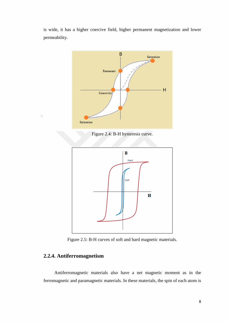
Hysteresis curve shows the change in the net magnetization of the ferromagnetic

material due to the change of the external magnetic field. By looking at the hysteresis

curve, it can be obtained that ferromagnetic materials will be saturated with how much

magnetic field the material exposed to. It is also understood from the hysteresis curve

for ferromagnetic materials that the material is soft or hard magnetic material. If it is

sufficient to apply small magnetic fields to achieve saturation, such materials are called

soft magnetic materials. Hysteresis curves of these soft materials are narrow and tall.

These materials are easily magnetized and their magnets can be eliminated. Very high

magnetic fields may be required to achieve the saturation value of some materials.

Such materials are also called hard magnetic materials. Hysteresis curves of these

materials are wide. These materials have a large permanent magnetization. These

magnetization can not be easily eliminated by applying an external field. Due to these

magnetization properties, hard magnetic materials are used as permanent magnets,

while soft magnetic materials are used in electromagnets and transformer cores [16].

In figure 2.5, hysteresis curves for soft and hard materials are compared [17].

Figure 2.4 shows the magnetization curve of a ferromagnetic material. The

magnetic field needs to be increased to a point to see the coercivity and magnetization

behaviour of a substance. When a sufficiently high magnetic field is applied to the

material, the magnetic domains are aligned and an additional increase does not change

the magnetization of the material since the material has reached saturation at this point.

When the magnetic field is reduced to zero, residual magnetization is seen in the

material. This is called remenant magnetization. The opposite magnetic field strength

to be applied to eliminate the permanent magnetization is called coercivity. The slope

of the B-H curve gives the permeability of the material.

If a material has a narrow hysteresis curve, it has a higher permeability, lower

permanent magnetization and a lower coercive field. However, if its hysteresis curve

8

is wide, it has a higher coercive field, higher permanent magnetization and lower

permeability.

Figure 2.4: B-H hysteresis curve.

Figure 2.5: B-H curves of soft and hard magnetic materials.

2.2.4. Antiferromagnetism

Antiferromagnetic materials also have a net magnetic moment as in the

ferromagnetic and paramagnetic materials. In these materials, the spin of each atom is

9

oriented in the opposite direction with the spin of the neighbor atoms. Therefore, if

there is no external magnetic field, the net magnetic moment is zero.

Figure 2.6: Behavior of magnetic moments of the antiferromagnetic materials.

2.2.5. Ferrimagnetism

In ferrimagnetic materials, the spins are in opposite directions but differently in

the spin sizes. Therefore, the net magnetic moment is equal to the difference in the

magnetic moments in the opposite directions. The magnetization of these materials is

similar to that of the ferromagnetic materials.

Figure 2.7: Behavior of magnetic moments of the ferrimagnetic materials.

10

3. MAGNETIC SENSORS AND THEIR

APPLICATIONS

Magnetic field has both magnitude and direction. Therefore, magnetic sensors

can be classified as vector or scalar by measuring the direction or magnitude of the

field. Scalar sensors measure the magnitude of the magnetic field but do not give

information about the direction of the field. Vector sensors can measure both the

magnitude and the vector components of the field.

If magnetic sensors are classified according to the field detection range, they can

be low field, medium field or high field magnetic sensors [18]. Low field sensors can

detect fields less than 1 microgauss. Sensors that detect fields between 1 microgauss

and 10 gauss are middle field sensors. The magnitude of the earth’s magnetic field is

around 0.5 gauss. High field sensors can measure fields greater than 10 gauss. Figure

3.1 shows the types of magnetic sensors and the ranges of fields they can detect [18].

Magnetic Sensor

Detectable Field Range (gauss)

10-8 10-4 100 104 108

Squid

Fiber-Optic

Optically Pumped

Nuclear Procession

Search-Coil

Anisotropic Magnetoresistive

Fluxgate

Magnetotransistor

Magnetodiode

Magneto-Optical

Giant Magnetoresistive

Hall Effect

Figure 3.1: Detection ranges for different magnetic sensors.

Earth’s Field

11

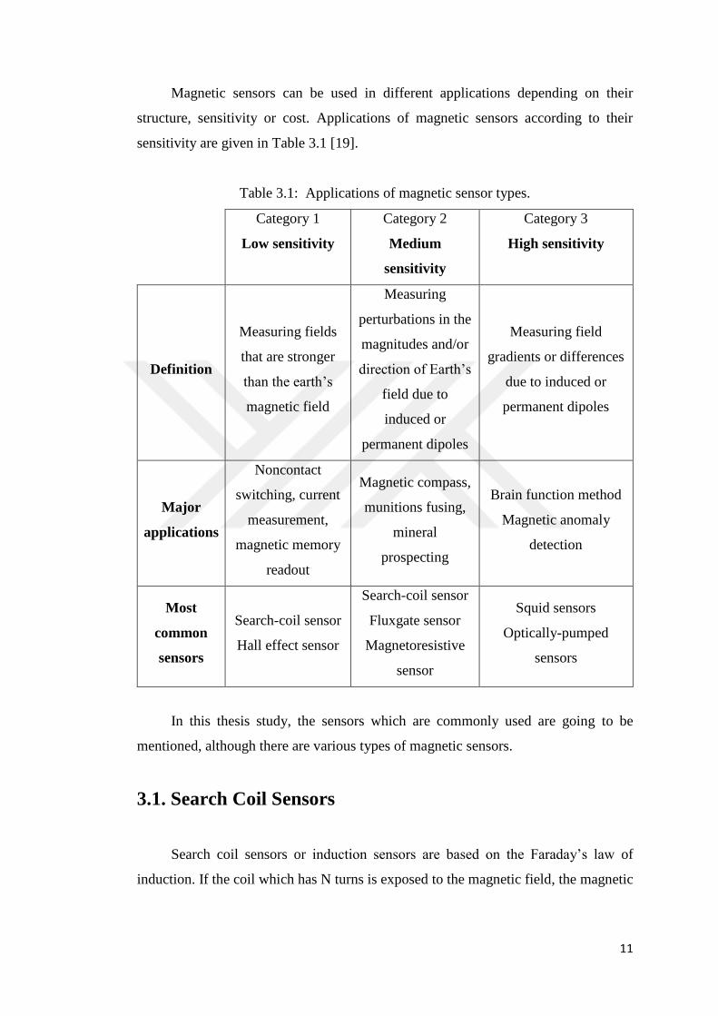
Magnetic sensors can be used in different applications depending on their

structure, sensitivity or cost. Applications of magnetic sensors according to their

sensitivity are given in Table 3.1 [19].

Table 3.1: Applications of magnetic sensor types.

Category 1

Low sensitivity

Category 2

Medium

sensitivity

Category 3

High sensitivity

Definition

Measuring fields

that are stronger

than the earth’s

magnetic field

Measuring

perturbations in the

magnitudes and/or

direction of Earth’s

field due to

induced or

permanent dipoles

Measuring field

gradients or differences

due to induced or

permanent dipoles

Major

applications

Noncontact

switching, current

measurement,

magnetic memory

readout

Magnetic compass,

munitions fusing,

mineral

prospecting

Brain function method

Magnetic anomaly

detection

Most

common

sensors

Search-coil sensor

Hall effect sensor

Search-coil sensor

Fluxgate sensor

Magnetoresistive

sensor

Squid sensors

Optically-pumped

sensors

In this thesis study, the sensors which are commonly used are going to be

mentioned, although there are various types of magnetic sensors.

3.1. Search Coil Sensors

Search coil sensors or induction sensors are based on the Faraday’s law of

induction. If the coil which has N turns is exposed to the magnetic field, the magnetic

12

flux through the coil changes and the coil generates voltage at the ends of the coil. The

induced voltage is given in Equation (3.1) and Equation (3.2).

Vi= -N𝑑Ф

𝑑𝑡 = -

𝑑(𝑁𝐴(𝑡)𝐵(𝑡))

𝑑𝑡= -

𝑑(𝑁𝐴(𝑡)𝜇˳𝜇ᵣ(𝑡)𝐻(𝑡))

𝑑𝑡 (3.1)

Vi= -NAµ˳H𝑑µᵣ(𝑡)

𝑑𝑡-NA𝜇˳µᵣ

𝑑𝐻(𝑡)

𝑑𝑡-Nµ˳µᵣH

𝑑𝐴(𝑡)

𝑑𝑡 (3.2)

In Equation (3.1), Ф shows the magnetic flux through the coil, A shows the cross

sectional area of the coil. The first term in Equation (3.2) is related to the fluxgate

effect [6]. The second term is the basic induction term. And the third term refers to

rotary coil sensors. Search-coil sensors measure the varying magnetic flux. They can

not measure DC fields. These sensors are vector sensors that measure both the

magnitude and the vector components of the magnetic field. Induction sensors can be

with air-core and ferromagnetic core [20]. The simplest induction sensor design is

shown in Figure 3.2 [21]. The winding number and the area of the coil and the

permeability of the ferromagnetic core material used are factors affecting the

sensitivity of the sensor [18].

Figure 3.2: The simplest induction sensor.

The search-coil sensors can measure the changing magnetic fields, from 1 Hz to

MHz frequencies [22]. These sensors are commonly used for current measurements,

detection of the magnetic anomaly in geophysics, magnetic recording techniques, in

13

electromagnetic compatibility (EMC) and electromagnetic interference (EMI)

measurements [4].

3.2. Hall Effect Sensors

The most commonly used magnetic field sensors are hall effect sensors. They

are suitable for measuring fields bigger than 1 mT [23]. Hall sensors and fluxgate

sensors are most commonly used for DC magnetic field measurements. Hall effect was

discovered by Edwin H. Hall [24]. This effect occurs on the moving charged particle.

The force formed on the charged particles is called the Lorentz force and this force is

given as:

�⃗�= -q(�⃗⃗�+�⃗�x�⃗⃗�) (3.3)

q is the electrical charge, v is the velocity of the particle, E is the electric field

intensity and B is the magnetic field intensity. The general operating principle of the

hall effect sensors is shown in Figure 3.3.

Figure 3.3: Schematic of the hall effect sensors.

Hall effect sensor consists of a thin strip of metal or semiconductor and

electrodes. If there is no magnetic field around the sensor, when a current is applied to

the input of the sensor, electrons move in a straight line from one side to the other side

of the strip. If there is some magnetic field that is perpendicular to the applied current,

14

it prevents the straight flow of the electrons. With the effect of the Lorentz force

electrons will deflect to down side of the strip. As a result, a potential difference occurs

between the other two sides of the strip. This potential difference is called as the Hall

voltage, VHall , that is shown in Equation (3.4).

VHall=khI . B

d (3.4)

Here, I, d and kh refers to the current, the thickness of the strip and the hall

coefficient, respectively. According to the Equation (3.4), when a constant current

flows through the conductor the hall voltage changes directly proportional to the

magnetic field. The value of the magnetic field can be measured by looking at the

voltage generated by the sensor. Hall sensors are less sensitive devices. But they are

used in many applications such as position sensing, current sensing and speed

detection since they are robust and simple to be manufactured [25].

3.3. Anisotropic Magnetoresistance Sensors (AMR)

Anisotropic magnetoresistance sensors are vector sensors that can measure the

amplitude and the direction of the magnetic field. AMR sensors can also sense DC

static fields. Magnetoresistance is the change in the resistivity of the material when an

external magnetic field is applied to it. The magnetoresistive effect in ferromagnetic

metals was observed by William Thomson in 1856 [26]. Thomson observed that the

resistivity of the ferromagnetic materials depend on the angle between the direction of

the applied electric current (I) and the magnetization orientation (M) of the material.

In these sensors to make a magnetoresistance, an iron-nickel alloy (about %80 iron

and %20 nickel), permalloy, is used since it shows magnetoresistance effect. Basic

configuration of an AMR sensor is shown in the Figure 3.4.

15

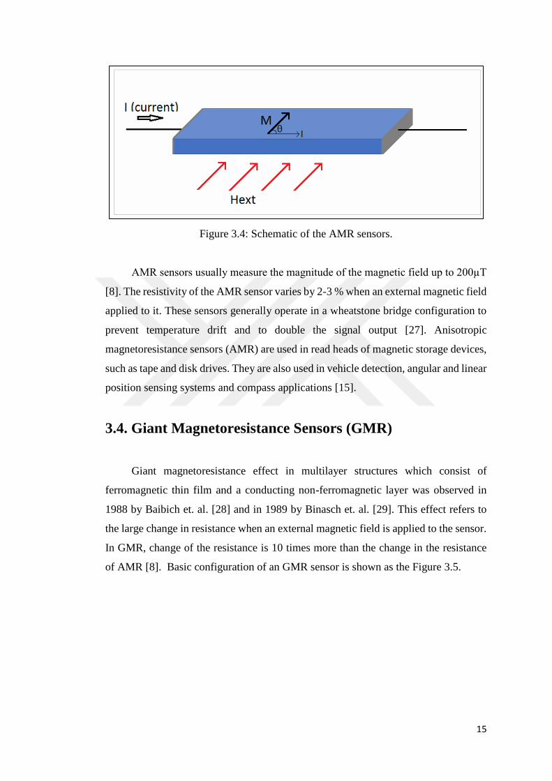
Figure 3.4: Schematic of the AMR sensors.

AMR sensors usually measure the magnitude of the magnetic field up to 200µT

[8]. The resistivity of the AMR sensor varies by 2-3 % when an external magnetic field

applied to it. These sensors generally operate in a wheatstone bridge configuration to

prevent temperature drift and to double the signal output [27]. Anisotropic

magnetoresistance sensors (AMR) are used in read heads of magnetic storage devices,

such as tape and disk drives. They are also used in vehicle detection, angular and linear

position sensing systems and compass applications [15].

3.4. Giant Magnetoresistance Sensors (GMR)

Giant magnetoresistance effect in multilayer structures which consist of

ferromagnetic thin film and a conducting non-ferromagnetic layer was observed in

1988 by Baibich et. al. [28] and in 1989 by Binasch et. al. [29]. This effect refers to

the large change in resistance when an external magnetic field is applied to the sensor.

In GMR, change of the resistance is 10 times more than the change in the resistance

of AMR [8]. Basic configuration of an GMR sensor is shown as the Figure 3.5.

16

Figure 3.5: Schematic of the multilayer GMR sensors.

In order to scattering of electrons, total layer must be thinner than the mean free

path of electrons [30]. When the magnetization moments are parallel, interface

scattering and total resistance occurs minimum. If the magnetization moments are anti-

parallel, then maximum resistance and interface scattering occur. GMR sensors are

used for many applications such as detection of vehicle, position sensing, magnetic

reading heads and nondestructive evaluation [4].

3.5. SQUID Sensors

SQUID (Superconducting Quantum Interference Device) is the most sensitive

sensor measuring magnetic field. For measuring pico tesla or smaller magnetic fields

SQUID sensors are preferred [23]. When the temperature falls below a certain value,

the resistance of the material becomes zero and shows the superconducting properties.

They can measure very small changes in magnetic flux. These sensors are vector

sensors. Their working principle is based on the magnetic flux quantization and

Josephson effect [31]. In 1962, it was foreseen by Brian Josephson that a pair of

electrons (Cooper pair) could tunnel through an insulating barrier seperating two

superconducting electrodes [32]. Josephson junction consists of two superconductor

and a thin insulator barrier. SQUID sensors can be RF or DC depending on whether

the applied current is alternating or dc. RF squid has a single josephson junction, while

the dc squid has two josephson junction. Although SQUIDs are very sensitive sensors,

17

they are more costly and consume more energy because they need to be cooled with

liquid hellium.

These sensors are used for magnetic anomaly detection, nondestructive

evaluation and medical applications such as electroencephalogram (EEG),

electrocardiogram (EKG) [4].

3.6. Fluxgate Sensors

Fluxgate sensors are high sensitive vector sensors. These sensors are used to

measure DC or low frequency AC magnetic fields. Fluxgate sensor consists of a soft

ferromagnetic core material and two coils, pick-up and excitation coils wrapped

around it [33]. Figure 3.6 shows basic structure of fluxgate sensors. Fluxgate sensors

work with the principle of periodically saturating a soft magnetic core. When the core

material is not yet saturated, the magnetic permeability increases and hence the

magnetic flux in the core increases (Figure 3.7.b). When AC current is applied to the

excitation coil, AC magnetic field occurs. Thanks to this field, the magnetic core

reaches saturation. Permeability of the magnetic core, which reach saturation by the

AC excitation field, decreases periodically and magnetic flux is gated (Figure 3.7.a).

The name of this sensor comes from gating the flux formed when the core is saturated.

Pick-up coil detects this periodic change in the permeability of the magnetic core. At

the output of the pick-up coil, a voltage is induced proportional to the measured field

and twice of the excitation frequency. Equation (3.1) and (3.2) given in Section 3.1 is

to be recalled again , the expression describing the operation of the fluxgate sensors is

given Equation (3.5).

V= NAµ˳H𝑑µᵣ(𝑡)

𝑑𝑡 (3.5)

If there is no external field, the voltage consists of odd harmonics on the signal.

This voltage is also symmetrical. When an external DC field is applied, the shifting in

the induced voltage occurs and the second and greater harmonic signal of the excitation

frequency is seen on the signal, as the time in which the core remains in saturation

increases in the direction in which this field is applied. Even harmonics of the signal

is proportional to the measured DC magnetic field. Between the even harmonics, the

18

intensity of the second harmonic signal is higher and this signal shows excellent linear

variation with the DC field to be measured.

If a resolution in the nanotesla range is desired, the fluxgate sensors will be the

best choice among other sensors [23]. While the SQUID sensors are also shown as

competitors to the fluxgate sensors, the SQUID sensors are high-power devices

because they need to be cooled with liquid helium. However the fluxgate sensors can

measure as low as 0.1 nano-tesla, while squid sensors can measure pico-tesla or lower

magnetic fields.

Figure 3.6: Schematic of the basic fluxgate sensors.

Figure 3.7: Fluxgate operation principle a) core is saturated b) core is not saturated.

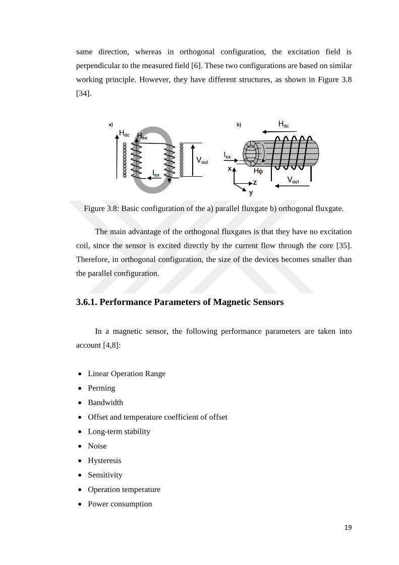
Fluxgate sensors can be in two different configurations, parallel or orthogonal.

In parallel configuration, both the excitation field and the measured field are in the

19

same direction, whereas in orthogonal configuration, the excitation field is

perpendicular to the measured field [6]. These two configurations are based on similar

working principle. However, they have different structures, as shown in Figure 3.8

[34].

Figure 3.8: Basic configuration of the a) parallel fluxgate b) orthogonal fluxgate.

The main advantage of the orthogonal fluxgates is that they have no excitation

coil, since the sensor is excited directly by the current flow through the core [35].

Therefore, in orthogonal configuration, the size of the devices becomes smaller than

the parallel configuration.

3.6.1. Performance Parameters of Magnetic Sensors

In a magnetic sensor, the following performance parameters are taken into

account [4,8]:

• Linear Operation Range

• Perming

• Bandwidth

• Offset and temperature coefficient of offset

• Long-term stability

• Noise

• Hysteresis

• Sensitivity

• Operation temperature

• Power consumption

20

• Demagnetization effect

• Sensor cost

The linear operation range in fluxgate sensors indicates the range in which the

voltage taken from the output of the pick-up coil of the sensor is linear with the applied

DC magnetic field. Perming is an offset change which occurs in the output of the

sensor when the sensor is exposed to a very high magnetic field. This change is called

the perming effect. Output of the sensor does not return to previous value,when this

field is removed. To reduce this effect in fluxgate sensors, the core of the sensor is well

saturated by applying a sufficiently large excitation current [36]. Bandwidth is a

frequency range where a sensor can detect input signals and generate output from

them. The stability of the magnetic sensors is expressed as the change in the offset

and sensitivity of the sensor depending on the time, temperature and the stress factor

of the ferromagnetic material [8]. Demagnetization effect is the parameter that causes

the field passing through the sensor to be smaller than the magnitude of the magnetic

field outside.

3.6.2. Choise of the Core Material

The core material used in fluxgate sensors greatly effects the performance of the

sensor [37]. When selecting the core material, it is important that the material has some

important magnetic properties [4]. Some of these features are as follows:

• High permeability

• Low coercivity

• Low saturation magnetization

• Low magnetostriction

• Low Barkhausen noise

• Smooth surface

• High electrical resistivity

Considering these properties, permalloy and cobalt based amorphous alloys are

often preferred as core materials in fluxgate sensors.

21

3.6.3. Miniaturized Fluxgate Sensors

Fluxgate sensors have high sensitivity but a bulky volume. Therefore, the

interest in miniaturized fluxgate sensors has increased recently, as it has smaller

dimensions, less power consumption, can be easily integrated into the electronic

circuits [9]. In addition to the small size, miniaturized sensors are required to reduce

the manufacturing costs [8]. Miniature fluxgate sensors are needed in many

applications such as sensor arrays, compasses, magnetic ink reading, navigation

systems, security sensors [4,8]. Nonetheless, the sensor’s noise increases, as the size

of the sensor is reduced [4]. Fluxgate sensors can be miniaturized by using PCB

technology or thin film technologies [38].

22

4. EXPERIMENTAL TECHNIQUES


Vibrating sample magnetometer is a device used to determine the magnetic

properties of the material. These devices are based on the principle of electromagnetic

induction. According to Faraday’s Law, if a magnetic flux density changes over time

in a conductor, a voltage is induced at the ends of that conductor. In order for the

magnetic flux density to change over time, either a time-varying magnetic field is

applied to the sample, or the sample is vibrated in the magnetic field. In this method

when the sample is vibrated under the magnetic field, the induced voltage value

changes directly proportional to the magnetization of this sample. The magnetization

of the material refers to the number of the magnetic moments in the per unit volume

of that material.

4.2. Photolithography

Photolithography is a process of transferring the geometric shapes in a mask onto

a substrate such as silicon or glass using ultraviolet light. The photolithography

processes are performed in clean rooms. The clean room is a working environment

that is free of dust and particles as much as possible, with constant humidity and

temperature. With the help of hepa filters in the clean room, the air is continuously

circulated and cleaned of dust.

The photolithography process is shown in Figure 4.1. First step of the

photolitography is substrate cleaning. Substrate is cleaned with the help of chemicals

such as aseton or alcohol. Then a photoresist is coated on substrate. Photoresist is a

sensitive material to light. It can be negative or positive. If the regions that exposed to

light are to be dissolved, positive photoresist is used, because the exposed regions

become more soluble in the developer process. On the contrary, if it is desired to

dissolve the regions that do not expose to light, negative photoresist is used. After the

photoresist coated by using spin coater, substrate is baked at certain temperature for a

while time. The purpose of prebaking is to ensure better adhesion of the photoresist to

23

the surface. After prebake process, substrate is exposed to UV light. The masks

designed using some drawing programs such as L-edit, Clewin or Autocad and printed

on chrome-coated glass using mask printer are used to transfer the desired shape to the

sample. The last process of the photolithography is development. This process allows

the dissolution of the photoresist in undesirable regions of the sample with the help of

a developer. Develop time varies according to the type and thickness of the photoresist

used.

Figure 4.1: Photolithography processes: a) Spinning of photoresist b) UV Exposure

c) After development for positive photoresist d) for negative photoresist.

In the fabrication of micro-nano devices, some techniques such as lift-off and

chemical etching are used to obtain the desired patterns together with lithography

techniques.

24

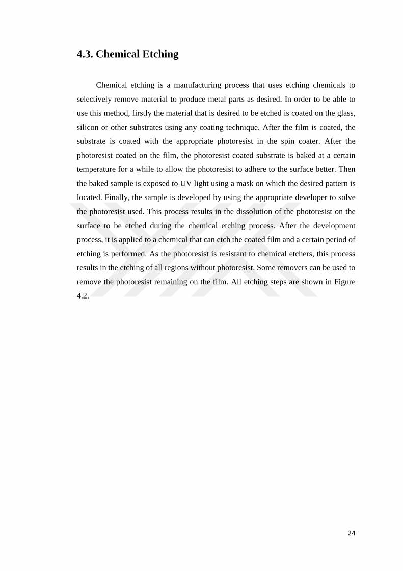
4.3. Chemical Etching

Chemical etching is a manufacturing process that uses etching chemicals to

selectively remove material to produce metal parts as desired. In order to be able to

use this method, firstly the material that is desired to be etched is coated on the glass,

silicon or other substrates using any coating technique. After the film is coated, the

substrate is coated with the appropriate photoresist in the spin coater. After the

photoresist coated on the film, the photoresist coated substrate is baked at a certain

temperature for a while to allow the photoresist to adhere to the surface better. Then

the baked sample is exposed to UV light using a mask on which the desired pattern is

located. Finally, the sample is developed by using the appropriate developer to solve

the photoresist used. This process results in the dissolution of the photoresist on the

surface to be etched during the chemical etching process. After the development

process, it is applied to a chemical that can etch the coated film and a certain period of

etching is performed. As the photoresist is resistant to chemical etchers, this process

results in the etching of all regions without photoresist. Some removers can be used to

remove the photoresist remaining on the film. All etching steps are shown in Figure

4.2.

25

Figure 4.2: Chemical Etching Processes: a) Coating of the film b) Spinning of

photoresist c) UV Exposure d) After development of positive photoresist e) negative

photoresist f) Etching of the metal film for positive photoresist g) for negative

photoresist h) removal of positive photoresist i) negative photoresist.

26

5. EXPERIMENTAL STUDIES

One of the most important parameters that affect the operation of the fluxgate

sensor is the magnetic properties of the core material to be used. Within the scope of

this study, as the core material Metglas 2714A, cobalt-based amorphous alloy with

low coercivity and high permeability, was used. Since the shape of the core material

significantly affected the sensitivity of the sensor, it was decided to produce meander

shaped core in order to increase the cross sectional area of the sensor core. The

meander-shaped core structure was produced using lithography and chemical etching

techniques. After the fabrication of the core was completed, the pick-up coil was

designed using copper wire. All fabrication and characterization processes were

performed for two different core materials which were annealed and not annealed.


The Vibrating Sample Magnetometer (VSM) system used for this thesis study is

Quantum Design PPMS 9T device located at Gebze Technical University, Physics

Department, Physical Property Measurement System (PPMS) Laboratory. This device

consists of a vacuum system, control panel, helium liquefaction unit, superconducting

magnet, VSM module, VSM engine. The sample is vibrated via the VSM engine. In

this study we have observed the M-H curves showing the magnetization of the

ferromagnetic material against applied magnetic field using VSM technique.

27

Figure 5.1: Vibrating sample magnetometer at Gebze Technical University, Physics

Department, Physical Property Measurement System (PPMS) Laboratory.

5.2. Photolithography Processes

Photolithography processes started by designing the mask on which it had the

desired shape to be transferred to the substrate. Firstly, 100 nm chrome layer was

coated on the mask glass. Then AZ 1505 photoresist was coated on the chrome layer.

Mask printing process was performed using Heidelberg DWL 66fs laser lithography

system, which is at Gebze Technical University, Nanotechnology Institute, Clean

Room Laboratory. The meander-shaped micro structures used in the chrome-coated

mask were designed using the Tanner Tools L-edit program. After printing of the

mask, develop process was made by using AZ 726 developer. Finally, the desired

shapes were obtained on the chrome-coated mask.

28

Figure 5.2: Mask printer device at Gebze Technical University, Nanotechnology


Before starting fabrication of the core material of the fluxgate sensor, the silicon

substrate was cleaned by vibrating in an ultrasonic bath for 5 minutes with acetone,

methanol and isopropanol, respectively. The silicon substrate was then dried with

nitrogen. Silicon wafer was preferred because its surface roughness is low compared

to glass. After making sure the substrate is clean and smooth, 23 micron thick cobalt-

based amorphous ribbon Metglas® 2714A was cut according to the size of the silicon

substrate and glued with epoxy adhesive on the Si-substrate so that there are no gaps

between them (Figure 5.5.a). The lithography process was started by applying SU-8

3005 negative photoresist coating on magnetic ribbon. Photoresist coating process was

performed using spin coater, which is at Gebze Technical University, Nanotechnology

Institute, Clean Room Laboratory. The appropriate parameters of the spin coater were

selected and the substrate was coated with 5 micron thick SU-8 3005 photoresist. Then

the sample was heated to 95°C for 150 seconds on the hot plate to enhance the adhesion

of the photoresist to surface of the ribbon. After the prebake process, the sample was

aligned with a chrome mask and exposed to the UV light. For the UV exposure process

SUSS MJB4 branded mask aligner, which is at Gebze Technical University,

Nanotechnology Institute, Clean Room Laboratory, was used. After exposure to UV

light, post exposure bake was made for 75 seconds at 95°C. Then the baked sample

29

was dissolved in the SU-8 developer. In all stages of photolithography, the images of

sample are shown in Figure 5.5.

Figure 5.3: Spin coater device at Gebze Technical University, Nanotechnology


Figure 5.4: Mask aligner device at Gebze Technical University, Nanotechnology


30

Figure 5.5: a) Ribbon glueing on silicon substrate b) Sample image after

development process.

5.3. Chemical Etching Process

After the photolithography process, there was only photoresist on the meander-

shaped core material on the substrate, while there was no protective layer on the other

parts of the surface of the ribbon. A chemical mixture had been prepared to etch these

regions without photoresist. This chemical mixture was composed of H2O, HNO3,

HCl, H2O2 acides (8:1:2:4). The ribbon was etched in these chemical solution for 5

minutes until the meander-shape was visible. After obtaining the core shape on the

silicon substrate, the Remover PG was used to remove the photoresist remaining on

the meander-shaped ribbon. The final version of the core fabrication is given in Figure

5.6.

31

Figure 5.6: Final image of the fluxgate sensor core after the etching process.

5.4. Sensor Design Processes

5.4.1. Core Design

Since orthogonal sensors do not have an excitation coil, excitation current will

be applied directly on the fabricated core material. As given in section 5.2 and section

5.3, the excitation part of the sensor was designed using photolithography and etching

techniques. Here, we wanted to work in an orthogonal structure that makes it easy to

work in miniature dimensions. In addition, the shape and size of the core material was

selected with reference to a study conducted in the literature in order to increase the

cross sectional area [14]. The width of each strip is 250 microns and the distance

between the strips is 150 microns. Meander shape consists of 8 turns. Design of the

core is shown in Figure 5.7.

Figure 5.7: Core design of the miniaturized fluxgate sensor.

32

5.4.2. Pick-up Coil Design

There is a need for an insulating assembly to disconnect the pick-up coils from

the core. If the pick-up coils were directly winded around the core, a short circuit would

be observed. Therefore, it is important for the sensor to ensure the insulation in

between the core material and the coils. In order to isolate the core shown in Figure

5.6 from the pick-up coil, a system with two plates was prepared as shown in Figure

5.8. Copper wire with a diameter of 0.11 mm was used for the pick-up coils. The pick-

up coil had 52 turns. Thus the design of the pick-up coil was realized. In all studies,

the effect of core material on sensor performance was investigated by changing the

properties of the core material used, provided that the pick-up coil assembly was the

same. The design processes of the pick-up coil of the fluxgate sensor were shown in

Figure 5.8 and Figure 5.9. To prevent the opening of the windings and protect the

sensor, the pick-up coils were wrapped with teflon tape.

Figure 5.8: One of the plate produced for pick-up coil windings.

Figure 5.9: Pick-up coil windings.

33

The meander shaped core material, which was fabricated on the silicon substrate

using photolithography and chemical etching production techniques was placed in the

pick-up coil carcass as shown in Figure 5.10.

Figure 5.10: Final image of miniaturized fluxgate sensor.

After receiving the contacts from the pads, the sensor was ready for

measurement. The same fabrication and design processes were performed for the

sensor having annealed Metglas 2714A core material.

5.4.3. Devices Used for Sensor Measurement

A measurement system is needed to evaluate the operation of fluxgate sensors.

The measurement system includes a function generator, a lock-in amplifier, a current

source, helmholtz coil or solenoid and signal analyzer. Schematic of the measurement

system used in the studies is given in Figure 5.11.

34

Figure 5.11: Measurement system of the fluxgate sensor.

5.4.3.1. Function Generator

An Agilent 33522A function generator was used for producing a sine wave

signal. AC current supply to magnetic core is provided by function signal generator.

5.4.3.2. Lock-in Amplifier

Usually, fluxgate sensors operate on the second harmonic detection principle. A

lock-in amplifier was needed to detect twice the frequency of the excitation signal. In

all measurements, Stanford SR844 RF lock-in amplifier was preferred because the

sensors that was produced operate at high frequency. The output voltage of the pick-

up coil is seen at the output of the lock-in amplifier.

5.4.3.3. Helmholtz Coil

A DC field source is needed to generate a uniform magnetic field. This field

source can be solenoid or helmholtz coil. A helmholtz coil with coil constant of 4,34

Oe/A was used to create the DC magnetic field to be measured.

35

5.4.3.4. Current Source

A current source was needed to produce the field with the helmholtz coil.

Keithley 220 programmable current source was used as the current source. This device

can produce current in the range of 1 nA with 100 mA.

5.4.3.5. Dynamic Signal Analyzer

A signal analyzer was needed to determine the noise level of the sensor. Agilent

35670 dynamic signal analyser was used in the measurement system. Magnetically

isolated environments were preferred for accurate results in noise measurements.

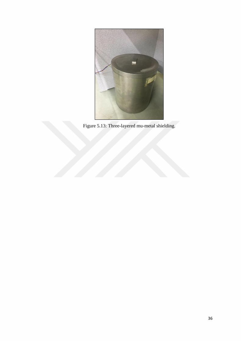
Noise measurements were made by leaving the sensor in a three-layered mu-metal

shields. The system used for sensor measurement is given in Figure 5.12. All sensor

measurements were performed in TÜBİTAK, National Metrology Institute, Magnetic

Measurements Laboratory.

Figure 5.12: Measurement devices for characterization of the sensors.

36

Figure 5.13: Three-layered mu-metal shielding.

37

6. RESULTS and DISCUSSION

In this section, the measurement results of the produced sensors are given.

Firstly, measurements were made by using Metglas 2714A cobalt-based amorphous

ribbon as core material. Then, using the same geometry of annealed Metglas 2714A

amorphous ribbon, the sensor was fabricated and measured in the same way. In

addition, sensors with non-annealed and annealed core were excited with 10 mA rms

and 80 mA rms excitation currents, respectively. The effect of the current value on the

sensitivity and noise of the sensor were observed. In addition, some improvement

studies had been carried out which may cause an increase in the performance of the

sensors.

6.1. Vibrating Sample Magnetometer (VSM) Measurement

Results

The VSM device was used to determine the magnetic properties of the core

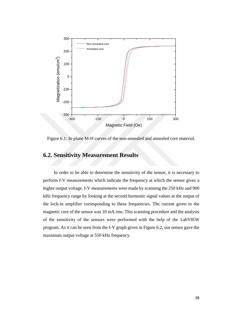
materials used. Measurements were performed at room temperature. Figure 6.1 shows

the comparison of the M-H curves of the annealed core material and the non-annealed

core material. When the ferromagnetic material is annealed under specific conditions,

the grain size increases and the lattice tension decreases [39]. This results in a

reduction in the coercivity of the ferromagnetic material. It is also expected that when

the materials are annealed, they will have a more uniform magnetic structure.

Therefore, as shown in Figure 6.1, the annealed core material has a lower coercivity.

In addition, the magnetic permeability of the annealed magnetic material is higher than

that of the non-annealed magnetic material.

38

-300 -150 0 150 300

-300

-200

-100

0

100

200

300

Mag

netizatio

n (

em

u/c

m3)

Magnetic Field (Oe)

Non-annealed core

Annealed core

Figure 6.1: In-plane M-H curves of the non-annealed and annealed core material.

6.2. Sensitivity Measurement Results

In order to be able to determine the sensitivity of the sensor, it is necessary to

perform f-V measurements which indicate the frequency at which the sensor gives a

higher output voltage. f-V measurements were made by scanning the 250 kHz and 900

kHz frequency range by looking at the second harmonic signal values at the output of

the lock-in amplifier corresponding to these frequencies. The current given to the

magnetic core of the sensor was 10 mA rms. This scanning procedure and the analysis

of the sensitivity of the sensors were performed with the help of the LabVIEW

program. As it can be seen from the f-V graph given in Figure 6.2, our sensor gave the

maximum output voltage at 550 kHz frequency.

39

200 300 400 500 600 700 800 900 1000

-0,10

-0,05

0,00

0,05

0,10

0,15

0,20

0,25

V2f (

mV

)

Frequency (Hz)

Figure 6.2: f-V measurement results.

The sensitivity of the fluxgate sensor is expressed as V/T. In fluxgate sensors,

second harmonic signals show excellent linearity with the DC field which is wanted

to be measured. Therefore, the linearity and slope of the 2f signal graphs corresponding

to the applied field are important to know the sensitivity value of the sensor.

First of all, the magnetic core was excited with a current of as low as 10 mA rms

at 550 kHz excitation frequency and sensitivity values were observed for the sensor

with non-annealed core. The sensitivity value of this sensor is 25.9 V/T, if the slope of

the curve in Figure 6.3 is linearly fitted.

When the same measurements were repeated for the sensor with annealed core

material, it was observed that the sensitivity value increased to 72.7 V/T. Figure 6.3

shows the effect of the annealing of the core material on the sensitivity of the sensor

when 10 mA rms current is applied to the sensor core.

40

-60 -40 -20 0 20 40 60

-3

-2

-1

0

1

2

3

V2f (

mV

)

Magnetic Field (T)

Non-annealed core

Annealed core

Figure 6.3: Sensitivity measurement results for the sensors with annealed and non-


In fluxgate sensors, the applied excitation current must be large enough to ensure

that the sensor is sufficiently saturated [40].

As another study, the excitation current was increased to 80 mA rms at same

excitation frequency and the effect of the excitation current on the sensitivity of the

sensor was observed. It was expected that the increase of the excitation current would

positively affect the operation of the sensor. When the slope of the graph of the second

harmonic signal voltage corresponding to the magnetic field in Figure 6.4 is

considered, the sensitivity value is 323 V/T for the sensor with non-annealed core

material. When the same excitation current is applied to the sensor having the annealed

core, the sensitivity was further increased to 387 V/T. The comparison of sensitivity

curves for the sensor with annealed and non-annealed core material are given in Figure

6.4.

41

-60 -40 -20 0 20 40 60

-20

-15

-10

-5

0

5

10

15

20

V2f (

mV

)

Magnetic Field (T)

Non-annealed core

Annealed core

Figure 6.4: Sensitivity measurement results for the sensors with annealed and non-


Figure 6.5 and Figure 6.6 show the effect of the applied excitation current on the

sensitivity of the sensor with the non-annealed and annealed core material,

respectively. It can be seen that the sensitivity of the sensors having annealed and non-

annealed core had increased depending on the excitation current. The second harmonic

signal values of the sensors show excellent linearity with the applied magnetic field.

42

-60 -40 -20 0 20 40 60

-15

-10

-5

0

5

10

15

V2f (

mV

)

Magnetic Field (T)

I= 10 mA rms, non-annealed core


Figure 6.5: Sensitivity measurement results for the sensors with non-annealed core

(f=550 kHz).

-60 -40 -20 0 20 40 60

-20

-15

-10

-5

0

5

10

15

20

V2f (

mV

)

Magnetic Field (T)

I= 10 mA rms, annealed core


Figure 6.6: Sensitivity measurement results for the sensors with annealed core

(f=550 kHz).

43

All sensitivity values obtained as a result of measurements are given in Table

6.1. According to this table, the maximum sensitivity value was reached in the sensor

with excited current of 80 mA rms and having annealed core.

Table 6.1: Sensitivity values for different conditions of the sensor.

Current Value Core Material Sensitivity

10 mA rms Non-annealed 25.9 V/T

10 mA rms Annealed 72.7 V/T

80 mA rms Non-annealed 323 V/T

80 mA rms Annealed 387 V/T

6.3. Noise Level Measurement Results

The noise level of the miniaturized fluxgate sensor is as important as its

sensitivity. Since the noise measurements of the sensor have to be done in a

magnetically isolated environment, the sensors were placed into three-layered mu-

metal shields. The magnetic field noise intensity values were obtained by dividing the

voltage noise density values read from the signal analyzer by the sensitivity values.

Voltage noise density values are expressed by V/√Hz. Therefore, the magnetic field

noise intensity values are expressed by T/√Hz. The noise levels of the sensors were

taken as the noise value corresponding to the 1 Hz frequency in all graphs.

Since the annealing process will eliminate the structural defects in the crystalline

structure of the ferromagnetic materials and obtain a homogeneous domain structure,

the sensor with the annealed core is expected to have a lower noise level. Figure 6.7

shows the noise levels of the annealed and non-annealed core sensors when the core

was supplied with 10 mA rms excitation current. When the noise values corresponding

to 1 Hz frequency were considered, this value was 6.89 nT/√Hz for the sensor with

non-annealed core. The noise level for the sensor with annealed core material has

decreased to 4.33 nT/√Hz.

When the excitation current was increased to 80 mA rms, the noise level of the

sensor with non-annealed core increased to 7.6 nT/√Hz as seen in Figure 6.8, while

the noise value of the sensor with annealed core remained almost the same as in the

previous current condition.

44

0 2 4 6 8 10 12 14

1

10

100

1000

10000N

ois

e (

nT

/H

z)

Frequency (Hz)

Non-annealed core

Annealed core

Figure 6.7: Noise level for the sensor with annealed core and non-annealed core

(f= 550 kHz, Iexc=10 mA).

0 2 4 6 8 10 12 14

1

10

100

1000

No

ise

(n

T/

Hz)

Frequency (Hz)

Non-annealed core

Annealed core

Figure 6.8: Noise level for the sensor with annealed core and non-annealed core

(f= 550 kHz, Iexc=80 mA).

45

Figure 6.9 and 6.10 show comparison of the noise levels of the sensors with non-

annealed and annealed core material depending on the excitation current applied to the

magnetic core, respectively. No significant changes were observed in the noise levels

of the sensors for two different excitation current values.

0 2 4 6 8 10 12 14

1

10

100

1000

10000

No

ise

(n

T/

Hz)

Frequency (Hz)



Figure 6.9: Noise measurements for the sensors with non-annealed core

(f= 550 kHz ).

46

0 2 4 6 8 10 12 14

1

10

100

1000

10000

Nois

e (

nT

/H

z)

Frequency (Hz)



Figure 6.10: Noise measurements of sensors with annealed core

(f= 550 kHz ).

Table 6.2 shows all noise levels for different core materials and different

excitation currents applied to core. According to this table, the minimum noise value

is also reached in the sensor with excited current of 80 mA rms and having annealed

core.

Table 6.2: Noise levels for different conditions of the sensor.

Current Value Core Material Noise

10 mA rms Non-annealed 6.89 nT/√Hz

10 mA rms Annealed 4.33 nT/√Hz

80 mA rms Non-annealed 7.66 nT/√Hz

80 mA rms Annealed 4.30 nT/√Hz

6.4. Effect of Current and Heat Treatment on Core Material

In this part of the thesis, we also desired to examine the effect of excitation

current and heat treatment applied to the core. Considering the sensitivity values of

our sensors with annealed and non-annealed core, it was thought that these results

47

should be improved. Two different studies were performed to investigate the

performance of the sensor. Firstly, since the sensor with the annealed core gave better

results in all of the previous measurements, it had been investigated whether better

sensitivity and noise value would be obtained when the excitation current for this

sensor was increased slightly so that the sensor was not damaged. Since there was no

current source with high frequency and high current output in our measurement

system, 120 mA current was applied to the sensor using a current source capable of

giving a maximum frequency of 200 kHz to observe the effect of much higher

excitation current on the sensor. Therefore, the same measurements were repeated by

applying 120 mA rms current at 200 kHz frequency to the core of the sensor having

annealed core. Sensitivity and noise level measurement results are given in Figure 6.11

and Figure 6.12, respectively. At this excitation current and frequency, there was no

improvement in the operation of the sensor, since the working frequency of our sensors

was 550 kHz. Therefore, not only increasing of excitation current but also the

excitation frequency of the sensor is significant for these sensors to work efficiently.

If these results were compared to the results when 80 mA rms excitation current

applied to the magnetic core, the sensitivity of the sensor decreased to 334.5 V/T, while

the noise level increased to 8.03nT/√Hz.

-60 -40 -20 0 20 40 60

-20

-15

-10

-5

0

5

10

15

20

V2f (

mV

)

Magnetic Field (T)

I= 120 mA rms, f=200 kHz, S=334.5 V/T

I= 80 mA rms, f=550 kHz, S=387.7 V/T

I= 10 mA rms, f=550 kHz, S=72.7 V/T

Figure 6.11: Comparison of sensitivity values of sensors with annealed core.

48

0 2 4 6 8 10 12 14

1

10

100

1000

10000

No

ise (

nT

/H

z)

Frequency (Hz)

I= 120 mA rms, f= 200 kHz, N= 8.03 nT/Hz



Figure 6.12: Comparison of noise levels of sensors with annealed core.

As another performance improvement study, in order to increase the output

signal strength of the sensors, the proper capacitor values to resonate the winding

systems were found and added to the pick-up coil of the sensors.

Figure 6.13: Addition of capacitor to the pick-up coils of the sensors with annealed

and non-annealed core (Iexc=10 mA rms).

For 10 mA rms excitation current, the capacitor to resonate the sensor was found

to be 3 nF. It is seen in Figure 6.14, along with the 3 nF capacitor connected to the

49

pick-up coil, the sensitivity of the sensor having non-annealed core increased slightly.

For the sensor with annealed core, adding 3 nF capacitor had increased the sensitivity

from 72.7 V/T to 76.9 V/T value, as seen in Figure 6.15.

-60 -40 -20 0 20 40 60

-1,5

-1,0

-0,5

0,0

0,5

1,0

1,5

V2f (

mV

)

Magnetic Field ()

Without capacitor

With 3 nF capacitor

Figure 6.14: Sensitivity measurement results of sensors with capacitor and without

capacitor for the sensor with non-annealed core (Iexc= 10 mA rms, f=550 kHz).

50

-60 -40 -20 0 20 40 60

-4

-3

-2

-1

0

1

2

3

4

V2f (

mV

)

Magnetic Field (T)

Without capacitor

With 3 nF capacitor

Figure 6.15: Sensitivity measurement results of sensors with capacitor and without

capacitor for the sensor with annealed core (Iexc= 10 mA rms, f=550 kHz).

-60 -40 -20 0 20 40 60

-4

-3

-2

-1

0

1

2

3

4

V2f (

mV

)

Magnetic Field (T)

Non-annealed core

Annealed core

Figure 6.16: Sensitivity measurements of sensors with 3 nF capacitor for the sensor

with annealed and non-annealed core (Iexc= 10 mA rms, f=550 kHz).

51

Figure 6.16 shows that the sensor with the annealed core had better sensitivity

even when the capacitor was connected to the pick-up coil.

Figure 6.17: Addition of capacitor to the pick-up coils of the sensors with annealed

and non-annealed core (Iexc= 80 mA rms).

When the excitation current was 80 mA rms, the proper capacitor value to

resonate the sensor was found to be 0.4 nF. It is seen from the slope of the curves in

Figure 6.18 that adding the capacitor value has increased the sensitivity of the sensor

having non-annealed core. For the sensor with annealed core, it has been observed that

the adding capacitor for this sensor also increased the sensitivity as shown in Figure

6.19.

52

-60 -40 -20 0 20 40 60

-15

-10

-5

0

5

10

15

V2f (

mV

)

Magnetic Field (T)

Without capacitor

With 0.4 nF capacitor

Figure 6.18: Sensitivity measurements of sensors with capacitor and without

capacitor for the sensor with non-annealed core (Iexc= 80 mA rms, f=550 kHz).

-60 -40 -20 0 20 40 60

-20

-15

-10

-5

0

5

10

15

20

V2f (

mV

)

Magnetic Field (T)

Without capacitor


Figure 6.19: Sensitivity measurements of sensors with capacitor and without

capacitor for the sensor with annealed core (Iexc= 80 mA rms, f=550 kHz).

53

In case the 0.4 nF capacitor have been added to the pick-up coils, the sensitivity

values of the sensor with annealed and non-annealed core are compared in Figure 6.20.

It is seen that the sensor with annealed core has better sensitivity even after adding the

proper capacitor.

-60 -40 -20 0 20 40 60

-20

-15

-10

-5

0

5

10

15

20

V2f (

mV

)

Magnetic Field (T)

Non-annealed core

Annealed core

Figure 6.20: Sensitivity measurements of sensors with 0.4 nF capacitor for the sensor

with annealed and non-annealed core (Iexc= 80 mA rms, f=550 kHz).

While the value of excitation current was 120 mA rms, the proper capacitor value

that will bring the system to resonance was found to be 5.6 nF. With the addition of

this capacitor value, the output signal strength of the sensor has increased. Therefore,

an improvement in the sensitivity of the sensor was also observed. As shown in Figure

6.21, the sensor had achieved a better sensitivity value when compared with other

sensors which were applied lower excitation current values. Furthermore, as shown in

Figure 6.22, it is seen that the noise level decreased after the capacitor was connected

to the pick-up coil for 120 mA rms excitation current. As a result, in the absence of the

desired high current source in the measurement system, the winding system was

resonated and the performance of the sensor with annealed core was improved at

different excitation frequency.

54

-60 -40 -20 0 20 40 60

-20

-15

-10

-5

0

5

10

15

20

V2f (

mV

)

Magnetic Field (T)

I=120 mA rms, f=200 kHz, S=439 V/T

I=80 mA rms, f=550 kHz, S=399 V/T

I=10 mA rms, f=550 kHz, S=77 V/T

Figure 6.21: Sensitivity comparison of the sensors having annealed core with


0 2 4 6 8 10 12 14

1

10

100

1000

10000

Nois

e (

nT

/H

z)

Frequency (Hz)

I= 120 mA rms, f=200 kHz, N=2.06 nT/Hz



Figure 6.22: Noise level comparison of the sensors having annealed core with


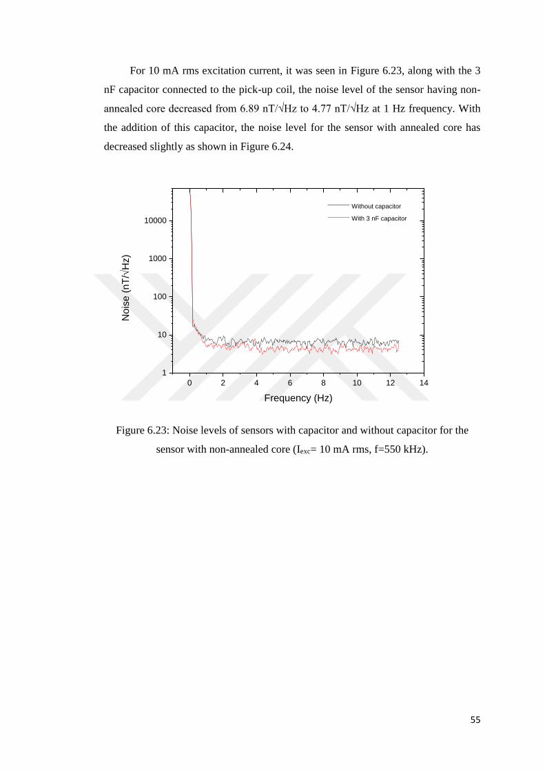
55

For 10 mA rms excitation current, it was seen in Figure 6.23, along with the 3

nF capacitor connected to the pick-up coil, the noise level of the sensor having non-

annealed core decreased from 6.89 nT/√Hz to 4.77 nT/√Hz at 1 Hz frequency. With

the addition of this capacitor, the noise level for the sensor with annealed core has

decreased slightly as shown in Figure 6.24.

0 2 4 6 8 10 12 14

1

10

100

1000

10000

No

ise

(n

T/

Hz)

Frequency (Hz)

Without capacitor

With 3 nF capacitor

Figure 6.23: Noise levels of sensors with capacitor and without capacitor for the


56

0 2 4 6 8 10 12 14

1

10

100

1000

10000

Nois

e (

nT

/H

z)

Frequency (Hz)

Without capacitor

With 3nF capacitor



In case the capacitor was added to the pick-up coils, the noise values of sensors

with annealed and non-annealed core were compared in Figure 6.25.

57

0 2 4 6 8 10 12 14

1

10

100

1000

10000N

ois

e (

nT

/H

z)

Frequency (Hz)

Non-annealed core

Annealed core

Figure 6.25: Noise levels of sensors with 3 nF capacitor for the sensor with annealed

and non-annealed core (Iexc= 10 mA rms, f=550 kHz).

When the excitation current was 80 mA rms, it is seen in Figure 6.26 that adding

the capacitor value has decreased the noise level of the sensor having non-annealed

core. For the sensor with annealed core, on the contrary, it is seen that the noise level

slightly increased after adding the capacitor as shown in Figure 6.27.

58

0 2 4 6 8 10 12 14

1

10

100

1000

Nois

e (

nT

/H

z)

Frequency (Hz)

Without capacitor




0 2 4 6 8 10 12 14

1

10

100

No

ise

(n

T/

Hz)

Frequency (Hz)

Without capacitor




59

0 2 4 6 8 10 12 14

1

10

100 N

ois

e (

nT

/H

z)

Frequency (Hz)

Non-annealed core

Annealed core

Figure 6.28: Noise levels of sensors with 0.4 nF capacitor for the sensor with


After adding 0.4 nF capacitor to the pick-up coils, the noise values of sensors

with annealed and non-annealed core are compared in Figure 6.28. It has been

observed that the noise level of the sensor which has non-annealed core is lower.

Table 6.3 and Table 6.4 show the sensitivity and noise values for the sensors

with different excitation current and core materials before and after adding the

capacitor.

Table 6.3: Sensitivity and noise values for sensors with different excitation current

and core materials before adding capacitors.

Excitation

Current Frequency

Core

Material Sensitivity Noise

10 mA rms 550 kHz Non-annealed 25.9 V/T 6.89 nT/√Hz

10 mA rms 550 kHz Annealed 72.7 V/T 4.33 nT/√Hz

80 mA rms 550 kHz Non-annealed 323 V/T 7.66 nT/√Hz

80 mA rms 550 kHz Annealed 387 V/T 4.30 nT/√Hz


60

Table 6.4: Sensitivity and noise values for sensors with different excitation current

and core materials after adding proper capacitors.

Excitation

Current Frequency

Core

Material Sensitivity Noise

10 mA rms 550 kHz Non-annealed 26.7 V/T 4.77 nT/√Hz

10 mA rms 550 kHz Annealed 76.9 V/T 4.05 nT/√Hz

80 mA rms 550 kHz Non-annealed 332 V/T 2.38 nT/√Hz



When all the results are thought together, the best sensitivity and noise values

are seen in the sensor with annealed core. There has been a significant increase in the

performance of the sensor since some properties of the magnetic core material have

been improved after heat treatment. In addition, it was seen that sensor sensitivity

increased with systematic increase of excitation current provided that the current

would be below the values that would not damage the sensor. It has also been observed

that increasing the excitation current to a certain value has a positive effect on the

performance of the sensor. Furthermore, the sensitivity value of the sensor increases

with the capacitor added to the sensor winding systems. Considering the noise levels,

if the number of layers of the mu-metal shielding used for noise measurements is

increased, the noise level of the sensors can be reduced to even lower value.

Looking at the literature, different core geometries were studied and maximum

378 V/T sensitivity was obtained using a multi-ring shaped core with 150 mA rms

excitation current using MEMS technologies [37]. In another study, it was observed

that the sensor having spiral shape core produced using MEMS technology reached a

maximum sensitivity of 117 V/T with 70 mA rms excitation current at 40 kHz [7]. In

addition, sensors with meander-shaped core were produced using MEMS

technologies, the sensitivity of the sensor that they produced has reached to 575 V/T

with using 90 mA rms excitation current at 500 kHz frequency [14]. In another study

about fluxgate sensors with orthogonal structure using CMOS fabrication processes, a

maximum sensitivity of 0.51 V/T with 100 mA peak excitation current at 100 kHz and

95 nT/√Hz at 1 Hz noise level have been reported [41]. Our sensor has reached a

maximum sensitivity of 439 V/T with using 120 mA rms excitation current at 200 kHz

frequency and 2.06 nT/√Hz noise at 1 Hz, after certain sensor improvement studies.

61

Considering the studies in the literature, our sensor performs better than many sensors,

but needs to be improved a little more.

The feature that highlights our sensors compared to the fluxgate sensors made in

many miniature dimensions is that our sensors are easier to fabricate and have lower

fabrication cost. We winded the pick-up coils directly onto the carcass around the core

rather than using any copper plating or micro fabrication techniques.

62

7. CONCLUSION

In this study, we designed and fabricated miniaturized orthogonal fluxgate

sensors. As the core material, magnetically soft materials which were annealed and

non-annealed form were used. We used photolithography and chemical etching

techniques to fabricate the sensors. In order to figure out the performance of the

designed sensors, we measured noise levels and sensitivities. Firstly, the sensors with

annealed and non-annealed core were driven by low excitation current. Secondly the

excitation current was increased. Noise and sensitivity of the sensors were examined.

As a result, it was observed that the sensors with annealed core and having higher

excitation current performed better.

To observe the behavior of the sensor when the excitation current is further

increased, higher excitation current was applied to the sensor with the annealed core

which gives better performance. Since there is no current source in our measurement

system that can drive higher current with high frequency, a lower frequency excitation

current was applied to this sensor. As a result of this performance improvement study,

there was no increase in the performance of the sensor. The conclusion is that not only

the increasing of the excitation current but also the excitation frequency has

importance on the performance of the sensor.

As another study, the pick-up coils of the sensors have been connected to the

appropriate capacitor values to resonate the winding systems. To conclude, the

performance of the sensors improved when a proper capacitor was added to the circuit.

Compared to the studies in the literature, our sensors perform better than many

miniaturized fluxgate sensors. Considering the dimensions of our sensors, they can be

easily integrated into many electronic systems. In this study, since it is seen that the

core material used in the sensor had a deep effect on the performance of the sensor, it

is aimed to improve the performance of the sensor by using different core materials in

future studies. It is also envisaged that improvements in sensor performance can be

achieved by optimizing the number of turns of the pick-up coil of the sensor and the

shape of the core material used.

63

REFERENCES

[1] Lenz J., Edelstein A., (2006), "Magnetic Sensors and Their Applications". IEEE Sensors Journal, 6 (3), 631–649.

[2] Thomas H. P., (1935), “Direction Responsive System”, US Patent 2,016,977.

[3] Aschenbrenner H., Goubau G., (1936), "Eine Anordnung zur Registrierung rascher magnetischer Störungen", Hochfrequenztech Electrokust, 47 (6), 177–181.

[4] Ripka P., (2001), "Magnetic Sensors and Magnetometers", 1st Edition, Boston: Artech House.

[5] Yağlıdere İ., (2018), "Novel Methods for Calculating the Demagnetization Factor of Ring-Core Fluxgate Sensors", Doktora Tezi, İstanbul Teknik Üniversitesi.

[6] Ripka P., (1992), "Review of Fluxgate Sensors", Sensors and Actuators A, 33, 129–141.

[7] Lei C., Lei J., Yang Z., Wang T., Zhou Y., (2013), "A Low Power Micro Fluxgate Sensor with Improved Magnetic Core", Microsystem Technologies, 19, 591–598.

[8] Zorlu Ö., (2008), "Orthogonal Fluxgate Type Magnetic Microsensors with Wide Linear Operation Range", Doctor of Philosophy Thesis, Institute of Microelectronics and Microsystems.

[9] Lei J., Lei C., Zhou Y.,(2012), "Micro Fluxgate Sensor Using Solenoid Coils Fabricated by MEMS Technology", Measurement Science Review, 12 (6), 286–289.

[10] Kubík J., Pavel L., Ripka P., Kašpar P., (2007), "Low-Power Printed Circuit Board Fluxgate Sensor", IEEE sensors journal, 7 (2), 179–183.

[11] Lu C. C., Huang J., Chiu P. K., Chiu S. L., Jeng J. T., (2014), "High-Sensitivity Low-Noise Miniature Fluxgate Magnetometers Using a Flip Chip Conceptual Design. Sensors", 14, 13815–13829.

[12] Lu C. C., Liu Y. T., Jhao F. Y., Jeng J. T., (2012), "Responsivity and Noise of a Wire-Bonded CMOS Micro-Fluxgate Sensor", Sensors Actuators A, 179, 39–43.

[13] Lu C. C., Huang W. S., Liu Y. T., Jeng J. T., (2011), "Design, Fabrication, and Characterization of a 3-D CMOS Fluxgate Magnetometer", IEEE Transactions on Magnetics, 47, 3752–3755.

[14] Zhi S., Feng Z., Guo L., Lei C., Zhou Y., (2017), "Investigation of a Novel MEMS Orthogonal Fluxgate Sensor Fabricated with Co-based Amorphous Ribbon Core", Sensors and Actuators A, 267, 121–126.

64

[15] Özkök E., (2017), "Düşük Manyetik Alan Algılama İçin Fluxgate Sensör Geliştirme ve Optimizasyonu", Yüksek Lisans Tezi, Yıldız Teknik Üniversitesi.

[16] Spaldin N. A., (2010), "Magnetic Materials: Fundamentals and Applications", 2nd Edition, Cambridge University Press.

[17] Callister W., Rethwisch D., (2009), "Materials Science and Engineering an Introduction", 8th Edition, Wiley.

[18] Caruso M. J., Bratland T, Smith C. H., Schneider R., (1998), "A New Perspective on Magnetic Field Sensing", Sensors, 15 (12), 34–45.

[19] Lenz J. E., (1990), "A Review of Magnetic Sensors", Proceeding of the IEEE, 78 (6), 973–989.

[20] Yağlıdere İ., (2010), "Fluxgate Tipi Hassas Manyetik Sensör Tasarımı", Yüksek Lisans Tezi, İstanbul Teknik Üniversitesi.

[21] Tumanski S., (2007), "Induction Coil Sensors - A review", Measurement Science and Technology, 18 (3), R31–R46.

[22] Edelstein A., (2007), “Advances in Magnetometry”, Journal of Physics : Condensed Matter, 19 (16), 165217.

[23] Ripka P., Tipek A., (2007), "Modern Sensors Handbook", UK.

[24] Hall E. H., (1879), "On a New Action of the Magnet on Electric Currents", American Journal of Mathematics , 2 (3), 287–292.

[25] Teresa M., Sileo L., Vittorio D. M., (2012), "Magnetic Field Sensors Based on Microelectromechanical Systems (MEMS) Technology", Magnetic Sensors - Principles and Applications, 103–124.

[26] Thomson W., (1857), "On the Electro-Dynamic Qualities of Metals:Effects of Magnetization on the Electric Conductivity of Nickel and of Iron", Proceedings Royal Society London, 8, 546–550.

[27] Jogschies L., Klaas D., Kruppe R., Rittinger J., Taptimthong P., Wienecke A., Rissing L., Wurz M. J., (2015), "Recent Developments of Magnetoresistive Sensors for Industrial Applications", Sensors, 15 (11), 28665–28689.

[28] Baibich M. N., Broto J. M., Fert A., Van Dau F.N., Petroff F., Eitenne P., Creuzet G., Friederich A., Chazelas J., (1988), "Giant Magnetoresistance of (001)Fe/(001)Cr Magnetic Superlattices", Physical Review Letters, 61 (21), 2472–2475.

[29] Binasch G., Grünberg P., Saurenbach F., Zinn W., (1989), "Enhanced Magnetoresistance in Layered Magnetic Structures with Antiferromagnetic Interlayer Exchange", Physical Review, 39 (7), 4828–4830.

[30] Hesse J., Gardner J. W., Gopel W., (2003), "Sensors for Automative Applications", Wiley.

[31] Granata C., Vettoliere A., (2016), "Nano Superconducting Quantum Interference Device: A Powerful Tool for Nanoscale Investigations". Physics Report, 614, 1–69.

65

[32] Josephson B. D., (1962), "Possible New Effects in Superconductive

Tunnelling", Physics Letters, 1 (7), 251–253.

[33] Can H., Svec J. P., Bydzovsky J., Svec S. P., Sözeri H., Topal U., (2017), "Systematic Optimization of the Sensing Properties of Ring-core Fluxgate Sensors with Different Core Diameters and Materials", Sensors and Actuators: A, 255, 94-103.

[34] Butta M., (2012), Orthogonal Fluxgates, Magnetic Sensors - Principles and Applications, Dr Kevin Kuang (Ed.), ISBN: 978-953-51-0232-8, http://www.intechopen.com/books/magnetic-sensorsprinciples-and-applications/orthogonal-fluxgates.

[35] Butta M., (2017), "Orthogonal Fluxgate Magnetometers", High Sensitivity Magnetometers, 1st edition, 19, 63–102, Springer International Publishing.

[36] Ripka, P., Janosec M., (2010), "Advances in Magnetic Field Sensors", IEEE Sensors Journal, 10 (6), 1108–1116.

[37] Lei J., Lei C., Zhou Y., (2013), "Analysis and Comparison of the Performance of MEMS Fluxgate Sensors with Permalloy Magnetic Cores of Different Structures", Measurement, 46, 710–715.

[38] Tumanski S., (2013), "Modern Magnetic Field Sensors-A Review", Przegląd Elektrotechniczny , 89 (10), 1–12.

[39] Sarkar A., Hembram S., Chatterjee S., Mallick A. B., (2018), "Effect of Annealing Treatments on the Magnetic Properties of FeCo/Cu Core Shell Nanostructures", Materials Today: Proceedings, 5, 745–751.

[40] Guo L., Wang C., Zhi S., Feng Z., Lei C., Zhou Y., (2017), "Wide Linearity Range and Highly Sensitive MEMS-based Micro-Fluxgate Sensor with Double-Layer Magnetic Core Made of Fe-Co-B Amorphous Alloy", Micromachines, 8 (12), 352.

[41] Zorlu Ö., Kejik P., Popovic R.S., (2007), “An Orthogonal Fluxgate-type Magnetic Microsensor with Electroplated Permalloy Core”, Sensors and Actuators A, 135, 43–49.

66

BIOGRAPHY

Fatmanur KOCAMAN was born in Erzurum, 1993. She completed her high

school education in Tevfik İleri Anatolian High School. She graduated from Electrical

and Electronics Engineering department at Atatürk University in 2016. She started her

Masters of Science degree in Nanotechnology Institute, Gebze Technical University.

As a part of her master of science education she took place as a scholarship in a

TÜBİTAK project of which number is 5155503 and is called “Development of

320x240 Pixel RGB AMOLED Avionics Displays”. She has been working as a

research assistant in Nanotechnology Institute, Gebze Technical University since

2017.

t.r. gebze technical university graduate school of

Documents