tracking with focus on the particle filter michael rubinstein idc
Post on 22-Dec-2015
220 views
TRANSCRIPT
Trackingwith focus on the particle filter
Michael RubinsteinIDC

Problem overview• Input
– (Noisy) Sensor measurements• Goal
– Estimate most probable measurement at time k using measurement up to time k’
k’<k: predictionk‘>k: smoothing
• Many problems require estimation of the state of systems that change over time using noisy measurements on the system
© Michael Rubinstein
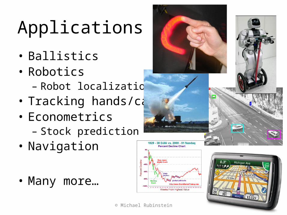
Applications• Ballistics• Robotics
– Robot localization• Tracking hands/cars/…• Econometrics
– Stock prediction• Navigation
• Many more…
© Michael Rubinstein
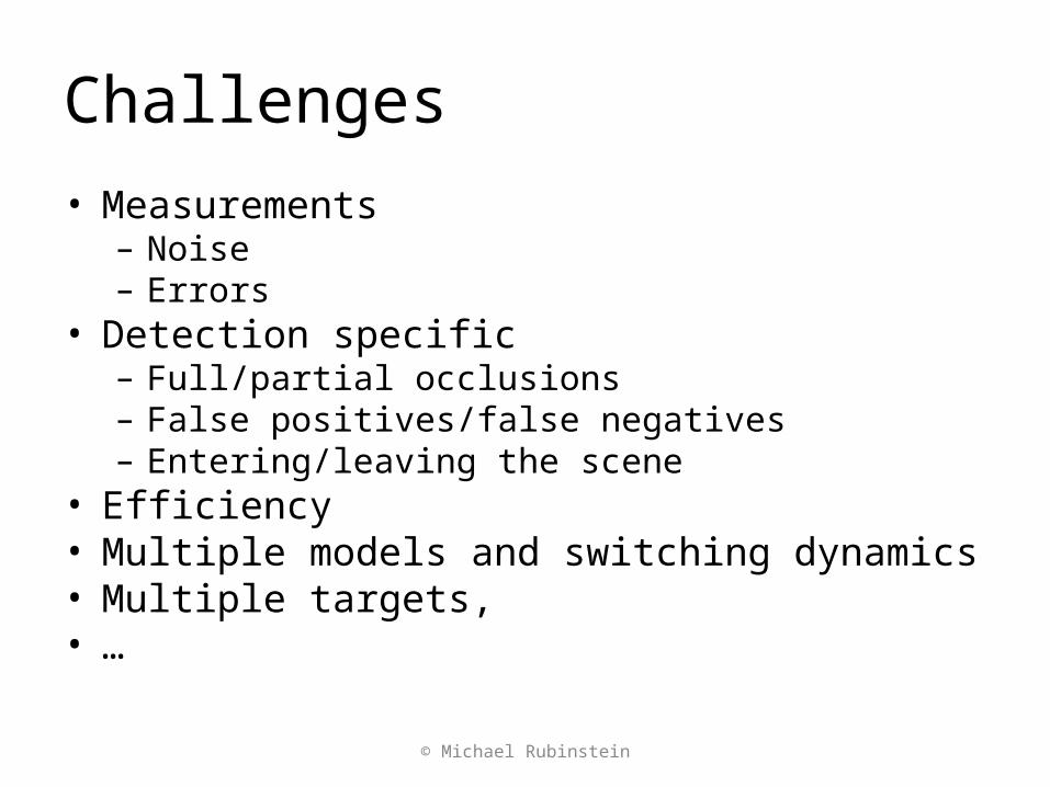
Challenges• Measurements
– Noise– Errors
• Detection specific– Full/partial occlusions– False positives/false negatives– Entering/leaving the scene
• Efficiency• Multiple models and switching dynamics• Multiple targets, • …
© Michael Rubinstein
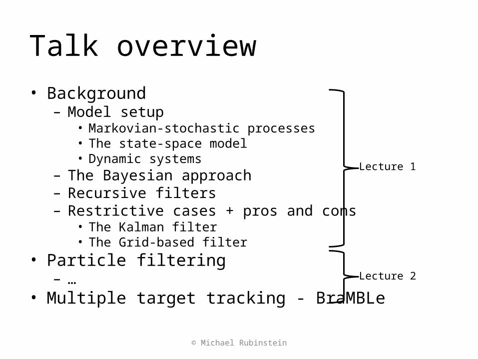
Talk overview• Background
– Model setup• Markovian-stochastic processes• The state-space model• Dynamic systems
– The Bayesian approach– Recursive filters– Restrictive cases + pros and cons
• The Kalman filter• The Grid-based filter
• Particle filtering– …
• Multiple target tracking - BraMBLe
© Michael Rubinstein
Lecture 1
Lecture 2

Stochastic Processes
• Deterministic process– Only one possible ‘reality’
• Random process– Several possible evolutions (starting point might be
known)– Characterized by probability distributions
• Time series modeling– Sequence of random states/variables– Measurements available at discrete times
© Michael Rubinstein
State space
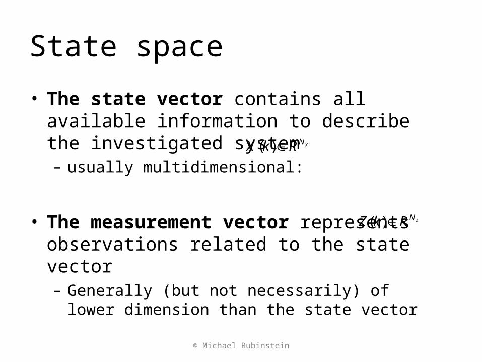
• The state vector contains all available information to describe the investigated system– usually multidimensional:
• The measurement vector represents observations related to the state vector– Generally (but not necessarily) of lower dimension
than the state vector
xNRkX )(
© Michael Rubinstein
zNRkZ )(
State space
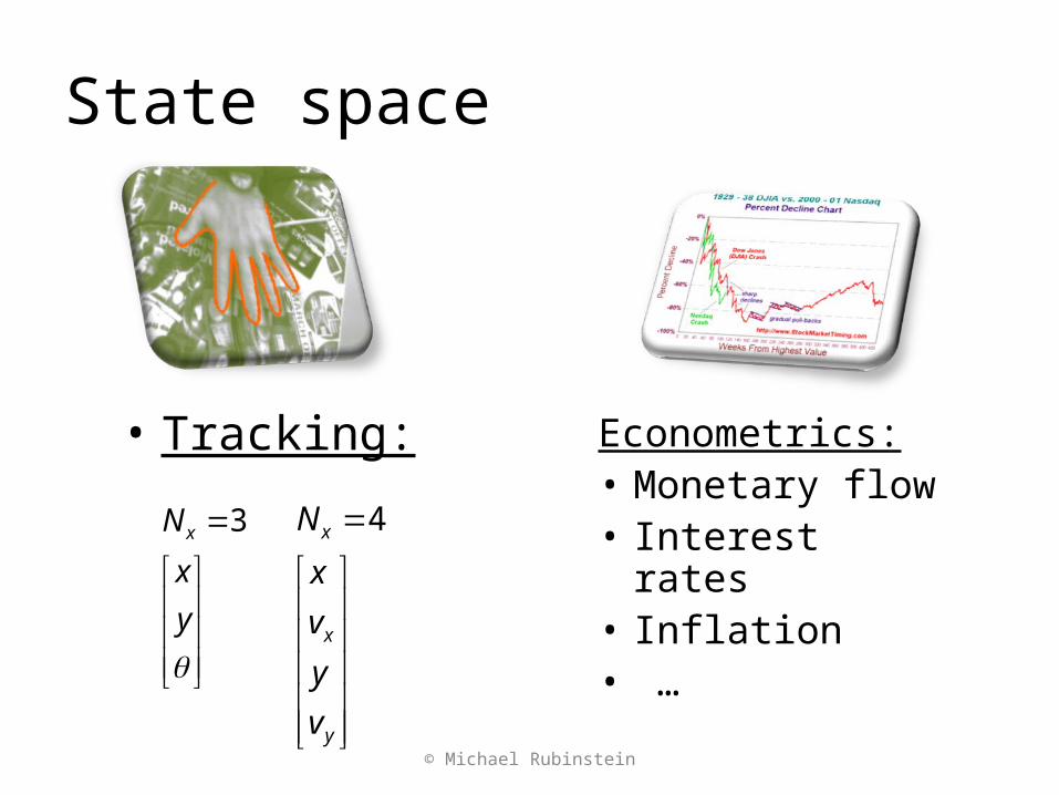
• Tracking: Econometrics:• Monetary flow• Interest rates• Inflation• …
y
x
N x 3
y
x
x
v
y
v
x
N 4
© Michael Rubinstein

(First-order) Markov process
• The Markov property – the likelihood of a future state depends on present state only
• Markov chain – A stochastic process with Markov property
0)],()(|)([Pr ]),()(|)(Pr[
hkxkXyhkXkssxsXyhkX
© Michael Rubinstein
k-1 k k+1 timexk-1 xk xk+1 States
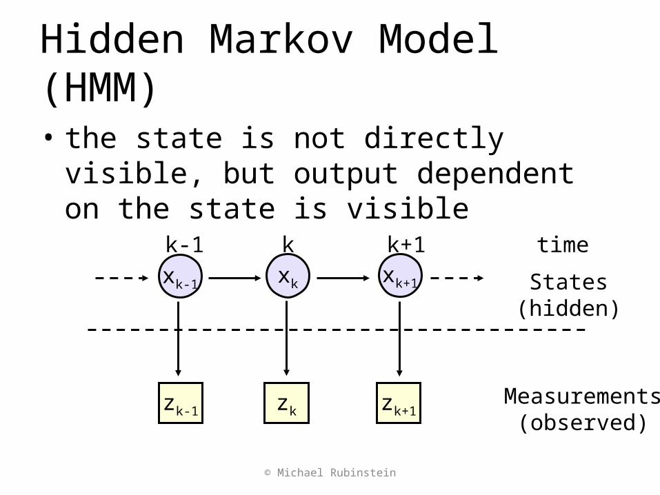
Hidden Markov Model (HMM)
• the state is not directly visible, but output dependent on the state is visible
© Michael Rubinstein
k-1 k k+1 timexk-1 xk xk+1 States
(hidden)
zk-1 zk zk+1Measurements
(observed)

Dynamic System
State equation: state vector at time instant k state transition function, i.i.d process noise
Observation equation:
observations at time instant kobservation function,i.i.d measurement noise
),( 1 kkkk vxfx
kxkf
xvx NNNk RRRf :
kv
),( kkkk wxhz kz
khkw
zwx NNNk RRRh :
© Michael Rubinstein
k-1 k k+1xk-1 xk xk+1
zk-1 zk zk+1
kf
kh
Stochastic diffusion
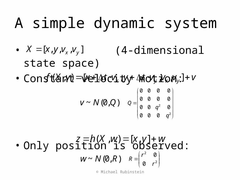
A simple dynamic system
• (4-dimensional state space) • Constant velocity motion:
• Only position is observed:
© Michael Rubinstein
],,,[ yx vvyxX
vvvvtyvtxvXf yxyx ],,,[),(
2
2
000
000
0000
0000
q
qQ),0(~ QNv
wyxwXhz ],[),(
),0(~ RNw
2
2
0
0
r
rR
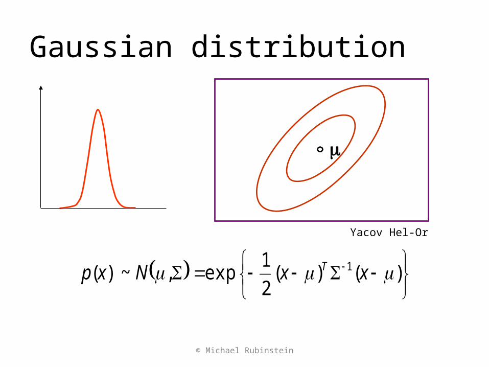
Gaussian distribution
© Michael Rubinstein
)()(
2
1exp,~)( 1 xxNxp T
Yacov Hel-Or
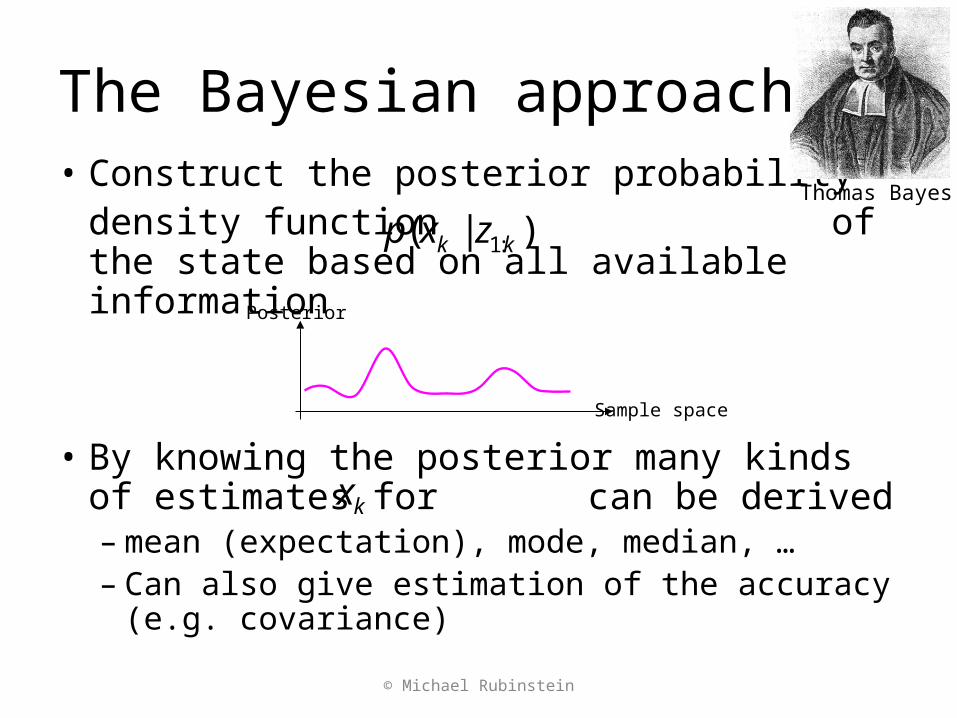
The Bayesian approach• Construct the posterior probability
density function of the state based on all available information
• By knowing the posterior many kinds of estimates for can be derived– mean (expectation), mode, median, …– Can also give estimation of the accuracy (e.g.
covariance)
)|( :1 kk zxp
© Michael Rubinstein
Thomas Bayes
kx
Sample space
Posterior
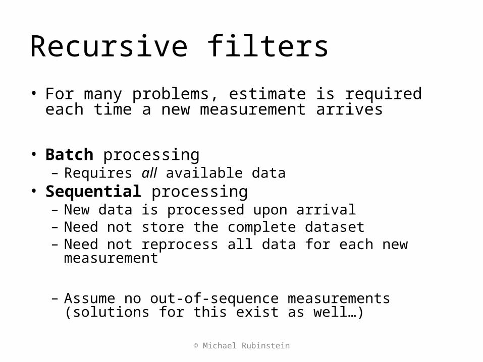
Recursive filters• For many problems, estimate is required each time a
new measurement arrives
• Batch processing– Requires all available data
• Sequential processing– New data is processed upon arrival– Need not store the complete dataset– Need not reprocess all data for each new measurement
– Assume no out-of-sequence measurements (solutions for this exist as well…)
© Michael Rubinstein
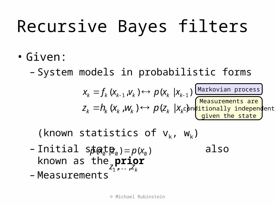
Recursive Bayes filters
• Given:– System models in probabilistic forms
(known statistics of vk, wk)
– Initial state also known as the prior– Measurements
© Michael Rubinstein
)|(),( 11 kkkkkk xxpvxfx
)|(),( kkkkkk xzpwxhz
Markovian process
Measurements are conditionally independent
given the state
)()|( 000 xpzxp
kzz ,,1
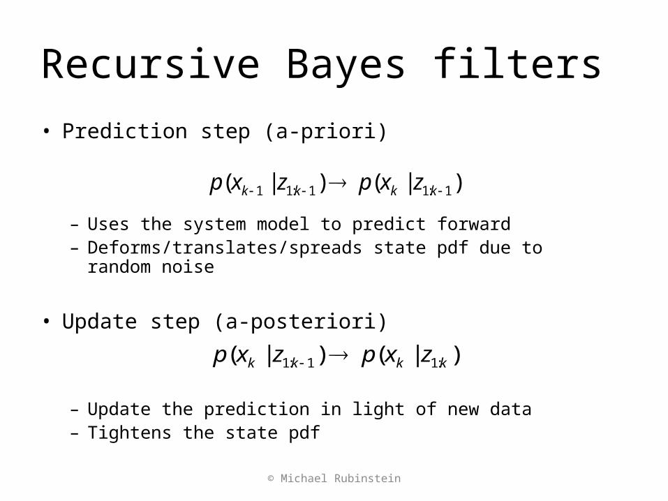
Recursive Bayes filters• Prediction step (a-priori)
– Uses the system model to predict forward– Deforms/translates/spreads state pdf due to random noise
• Update step (a-posteriori)
– Update the prediction in light of new data– Tightens the state pdf
)|()|( 1:11:11 kkkk zxpzxp
)|()|( :11:1 kkkk zxpzxp
© Michael Rubinstein

General prediction-update framework
• Assume is given at time k-1• Prediction:
• Using Chapman-Kolmogorov identity + Markov property
)|( 1:11 kk zxp
11:1111:1 )|()|()|( kkkkkkk dxzxpxxpzxp (1)
© Michael Rubinstein
Previous posteriorSystem model

General prediction-update framework
• Update step
Where
)|(
)|()|(
)|(
)|(),|(
),|()|(
1:1
1:1
1:1
1:11:1
1:1:1
kk
kkkk
kk
kkkkk
kkkkk
zzp
zxpxzp
zzp
zxpzxzp
zzxpzxp
kkkkkkk dxzxpxzpzzp )|()|()|( 1:11:1
(2)
)|(
)|(),|(),|(
CBp
CApCABpCBAp
© Michael Rubinstein
evidence
priorlikelihood
Measurement model
Currentprior
Normalization constant
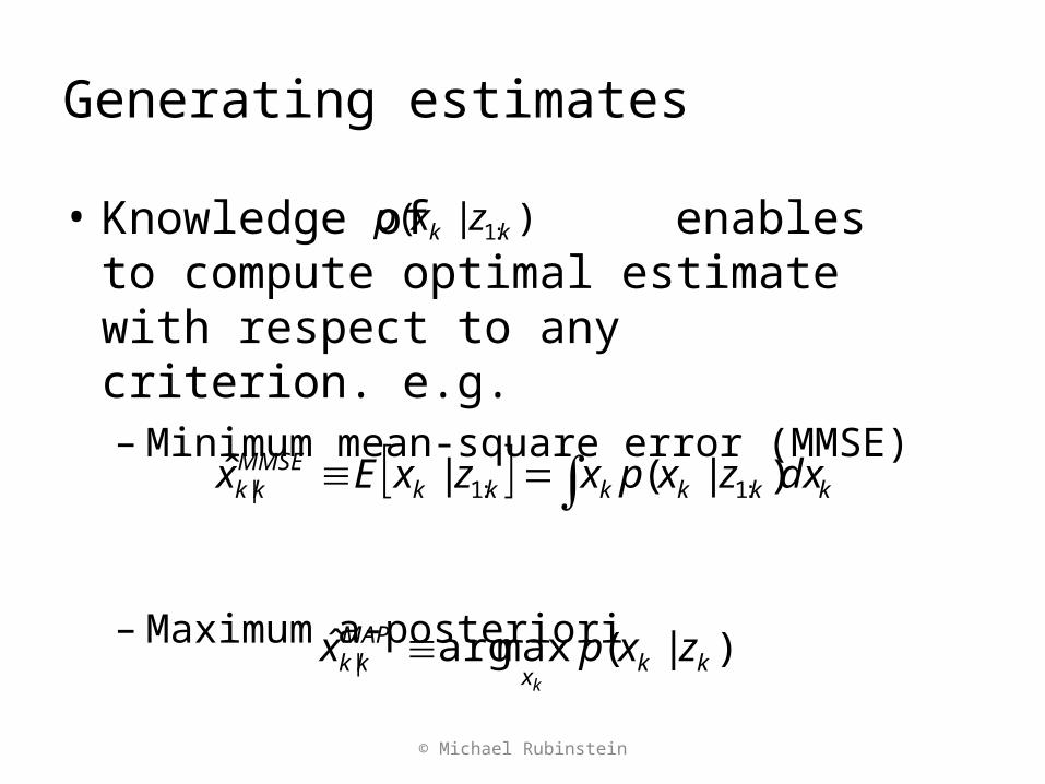
Generating estimates
• Knowledge of enables to compute optimal estimate with respect to any criterion. e.g.– Minimum mean-square error (MMSE)
– Maximum a-posteriori
kkkkkkMMSEkk dxzxpxzxEx )|(|ˆ :1:1|
)|( :1 kk zxp
)|(maxargˆ | kkx
MAPkk zxpx
k
© Michael Rubinstein
General prediction-update framework
So (1) and (2) give optimal solution for the recursive estimation problem!
• Unfortunately no… only conceptual solution– integrals are intractable…– Can only implement the pdf to finite representation!
• However, optimal solution does exist for several restrictive cases
© Michael Rubinstein

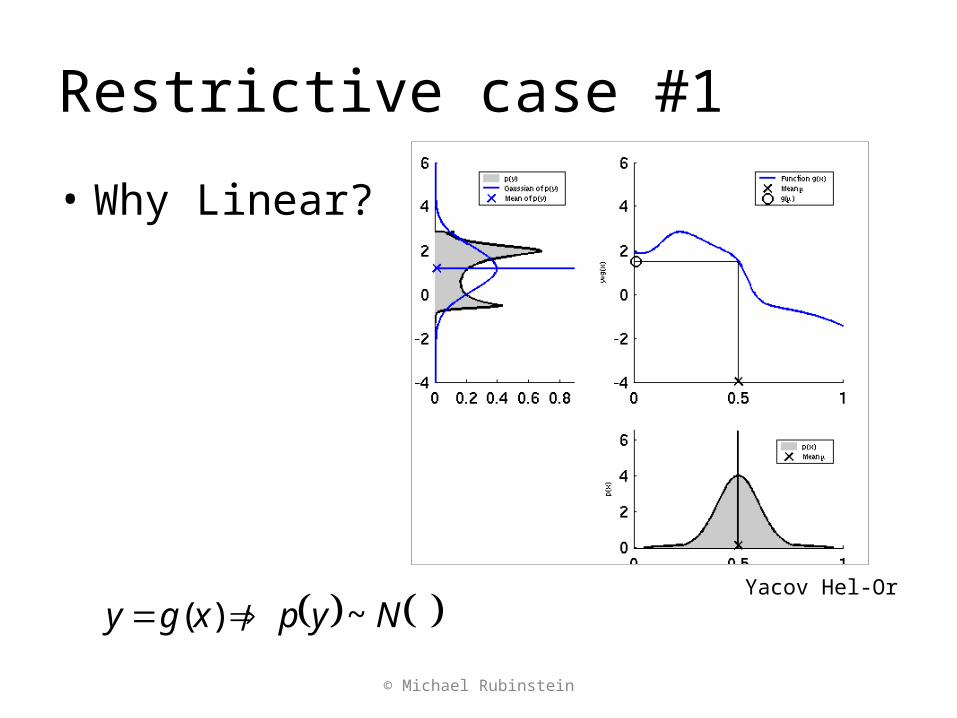
Restrictive case #1
• Posterior at each time step is Gaussian– Completely described by mean and covariance
• If is Gaussian it can be shown that is also Gaussian provided that:– are Gaussian– are linear
)|( 1:11 kk zxp
)|( :1 kk zxp
kk wv ,
kk hf ,
© Michael Rubinstein
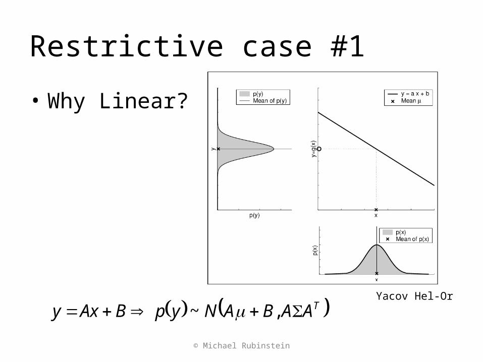
Restrictive case #1
© Michael Rubinstein
• Why Linear?
Yacov Hel-Or
TAABANypBAxy ,~
Restrictive case #1
© Michael Rubinstein
• Why Linear?
Yacov Hel-Or
Nypxgy ~)(
Restrictive case #1
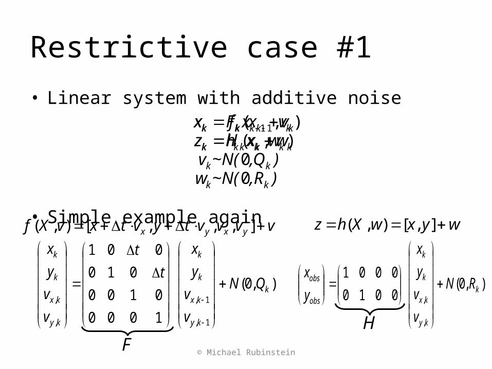
• Linear system with additive noise
• Simple example again
© Michael Rubinstein
),(),( 1
kkkk
kkkk
wxhzvxfx
),R~N(w),Q~N(vwxHzvxFx
kk
kk
kkkk
kkkk
00
1
vvvvtyvtxvXf yxyx ],,,[),( wyxwXhz ],[),(
),0(
1000
0100
010
001
1,
1,
,
,k
ky
kx
k
k
ky
kx
k
k
QN
v
v
y
x
t
t
v
v
y
x
),0(0010
0001
,
,k
ky
kx
k
k
obs
obs RN
v
v
y
x
y
x
FH
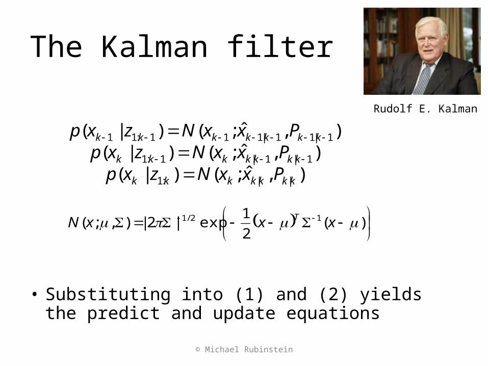
The Kalman filter
• Substituting into (1) and (2) yields the predict and update equations
),ˆ;()|(),ˆ;()|(
),ˆ;()|(
||:1
1|1|1:1
1|11|111:11
kkkkkkk
kkkkkkk
kkkkkkk
PxxNzxpPxxNzxpPxxNzxp
)(
2
1exp|2|),;( 12/1 xxxN T
Rudolf E. Kalman
© Michael Rubinstein
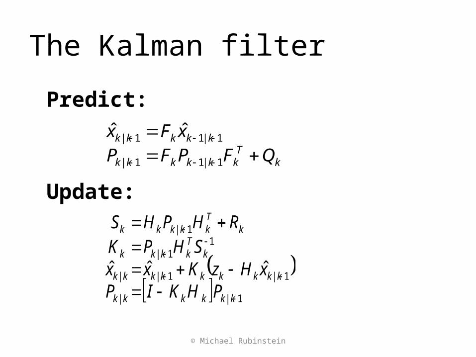
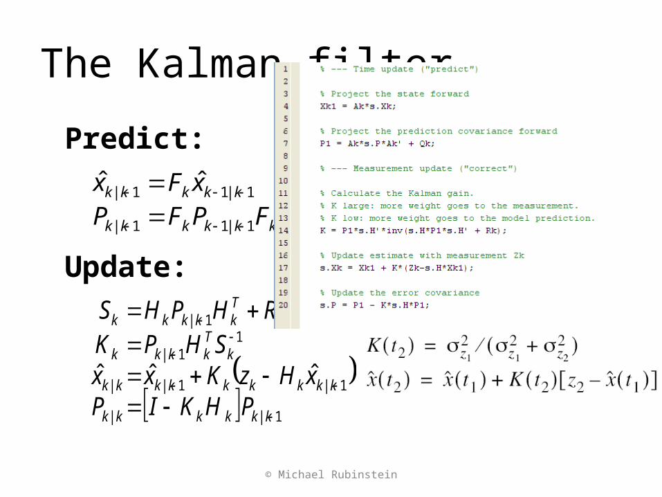
The Kalman filter
Predict:
Update:
© Michael Rubinstein
kTk|kkkk|k
|kkkk|k
QFPFPxFx
111
111 ˆˆ
1
11
11
1
ˆˆˆ
k|kkkk|k
k|kkkkk|kk|k
kTkk|kk
kTkk|kkk
PHKIPxHzKxx
SHPKRHPHS
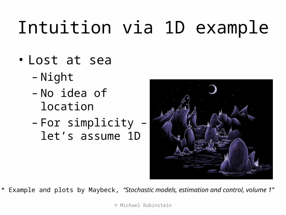
Intuition via 1D example
• Lost at sea– Night– No idea of location– For simplicity – let’s
assume 1D
© Michael Rubinstein
* Example and plots by Maybeck, “Stochastic models, estimation and control, volume 1”
Example – cont’d
• Time t1: Star Sighting– Denote x(t1)=z1
• Uncertainty (inaccuracies, human error, etc)– Denote 1 (normal)
• Can establish the conditional probability of x(t1) given measurement z1
© Michael Rubinstein
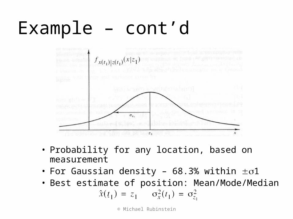
Example – cont’d
• Probability for any location, based on measurement• For Gaussian density – 68.3% within 1• Best estimate of position: Mean/Mode/Median
© Michael Rubinstein
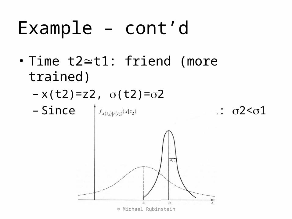
Example – cont’d
• Time t2t1: friend (more trained)– x(t2)=z2, (t2)=2– Since she has higher skill: 2<1
© Michael Rubinstein
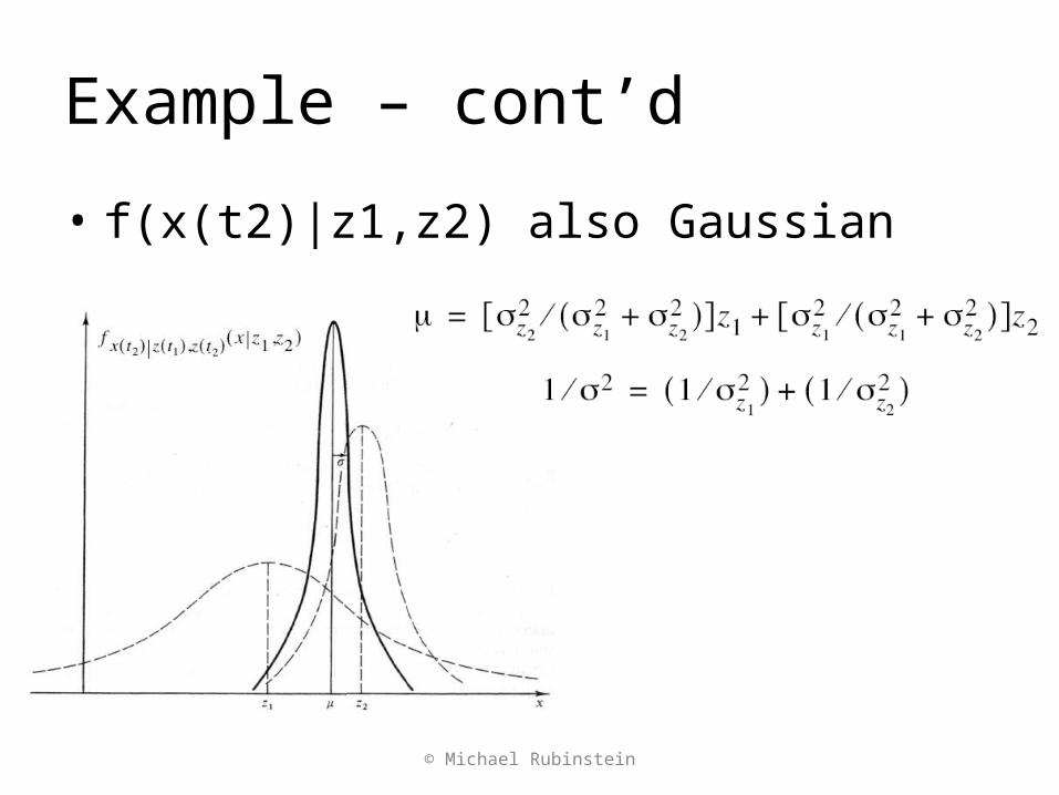
Example – cont’d
• f(x(t2)|z1,z2) also Gaussian
© Michael Rubinstein
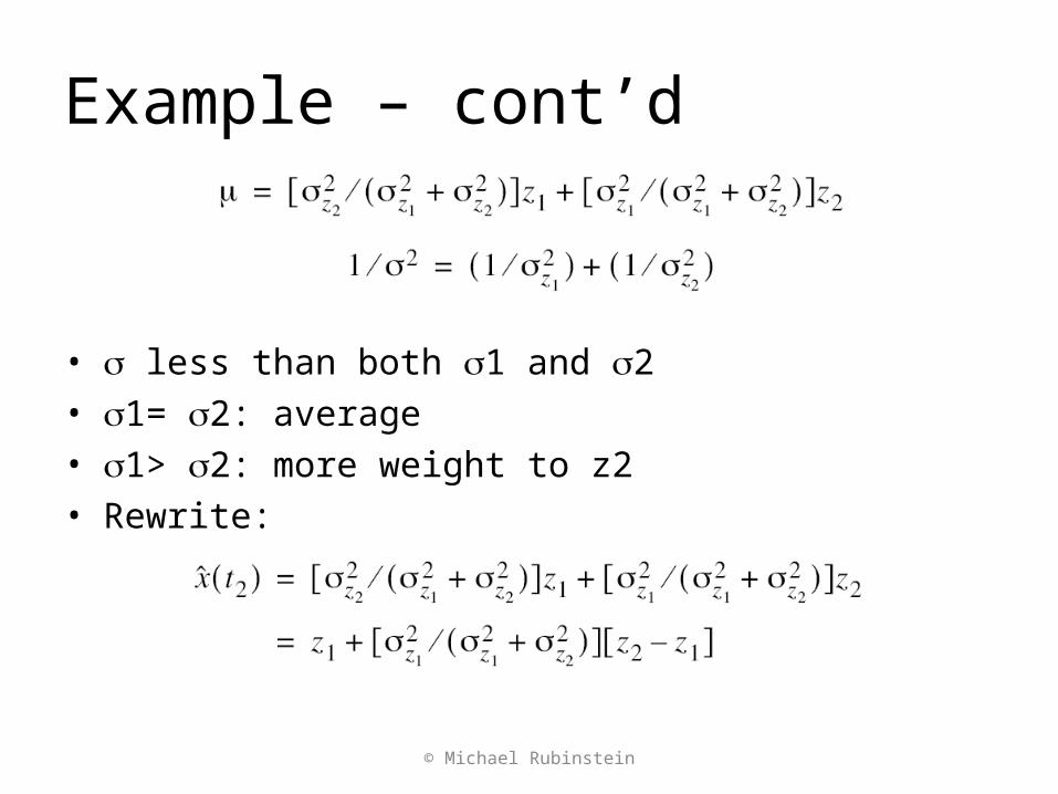
Example – cont’d
• less than both 1 and 2• 1= 2: average• 1> 2: more weight to z2• Rewrite:
© Michael Rubinstein
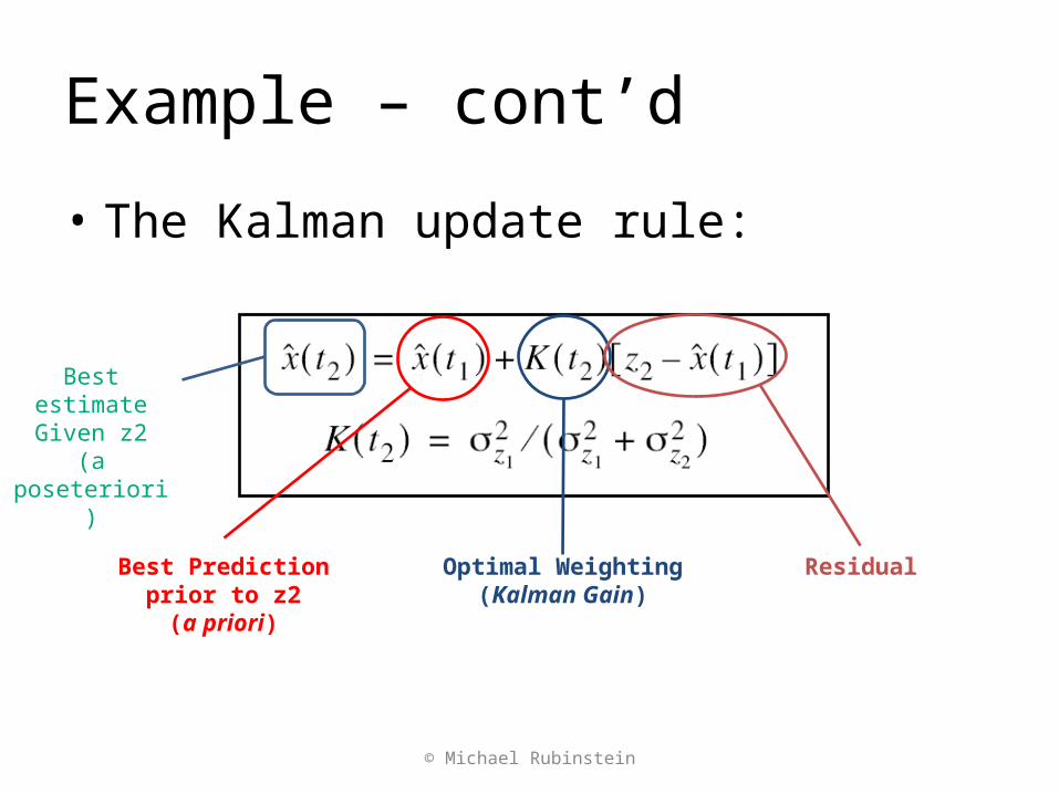
Example – cont’d
• The Kalman update rule:
Best Prediction prior to z2(a priori)
Optimal Weighting(Kalman Gain)
Residual
Best estimate Given z2
(a poseteriori)
© Michael Rubinstein
The Kalman filter
Predict:
Update:
kTk|kkkk|k
|kkkk|k
QFPFPxFx
111
111 ˆˆ
1
11
11
1
ˆˆˆ
k|kkkk|k
k|kkkkk|kk|k
kTkk|kk
kTkk|kkk
PHKIPxHzKxx
SHPKRHPHS
© Michael Rubinstein
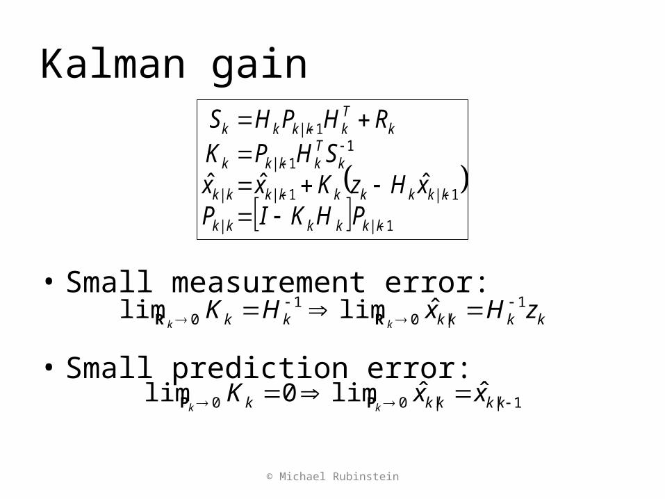
Kalman gain
• Small measurement error:
• Small prediction error:
© Michael Rubinstein
1
11
11
1
ˆˆˆ
k|kkkk|k
k|kkkkk|kk|k
kTkk|kk
kTkk|kkk
PHKIPxHzKxx
SHPKRHPHS
kkkkkk zHxHKkk
1|0
10 ˆlimlim
RR
1||00 ˆˆlim0lim kkkkk xxKkk PP

The Kalman filter• Pros
– Optimal closed-form solution to the tracking problem (under the assumptions)
• No algorithm can do better in a linear-Gaussian environment!
– All ‘logical’ estimations collapse to a unique solution– Simple to implement– Fast to execute
• Cons– If either the system or measurement model is non-
linear the posterior will be non-Gaussian
© Michael Rubinstein

Restrictive case #2
• The state space (domain) is discrete and finite• Assume the state space at time k-1 consists of
states • Let be the conditional
probability of the state at time k-1, given measurements up to k-1
sik Nix ..1,1
ikkk
ikk wzxx 1|11:111 )|Pr(
© Michael Rubinstein
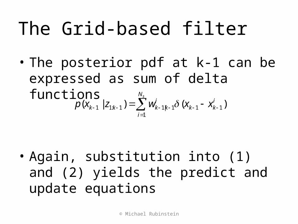
The Grid-based filter
• The posterior pdf at k-1 can be expressed as sum of delta functions
• Again, substitution into (1) and (2) yields the predict and update equations
sN
i
ikk
ikkkk xxwzxp
1111|11:11 )()|(
© Michael Rubinstein
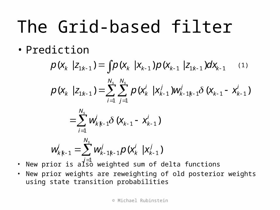
The Grid-based filter• Prediction
• New prior is also weighted sum of delta functions• New prior weights are reweighting of old posterior weights using state
transition probabilities
11:1111:1 )|()|()|( kkkkkkk dxzxpxxpzxp (1)
s
s s
N
i
ikk
ikk
N
i
N
j
ikk
jkk
jk
ikkk
xxw
xxwxxpzxp
1111|
1 1111|111:1
)(
)()|()|(
sN
j
jk
ik
jkk
ikk xxpww
111|11| )|(
© Michael Rubinstein
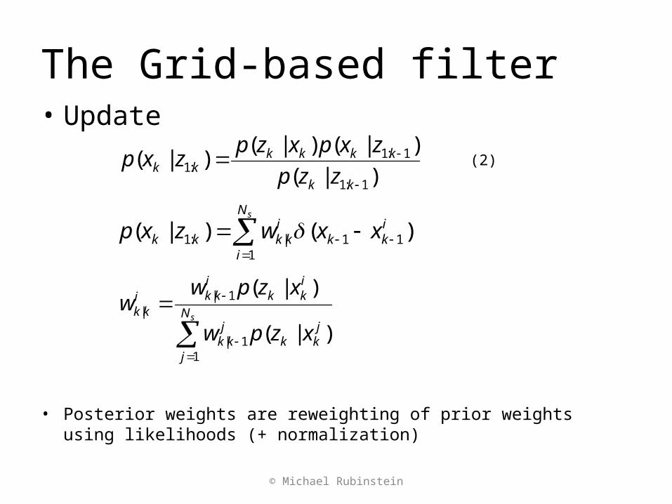
The Grid-based filter• Update
• Posterior weights are reweighting of prior weights using likelihoods (+ normalization)
sN
i
ikk
ikkkk xxwzxp
111|:1 )()|(
sN
j
jkk
jkk
ikk
ikki
kk
xzpw
xzpww
11|
1||
)|(
)|(
)|(
)|()|()|(
1:1
1:1:1
kk
kkkkkk zzp
zxpxzpzxp (2)
© Michael Rubinstein
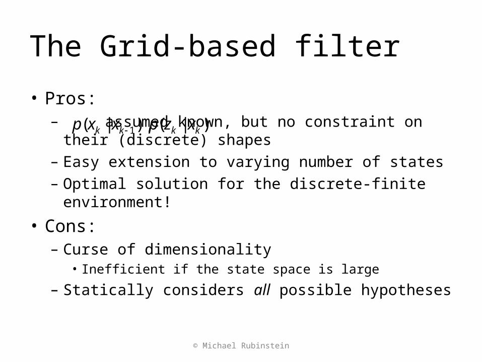
The Grid-based filter
• Pros:– assumed known, but no
constraint on their (discrete) shapes– Easy extension to varying number of states– Optimal solution for the discrete-finite environment!
• Cons:– Curse of dimensionality
• Inefficient if the state space is large
– Statically considers all possible hypotheses
)|(),|( 1 kkkk xzpxxp
© Michael Rubinstein
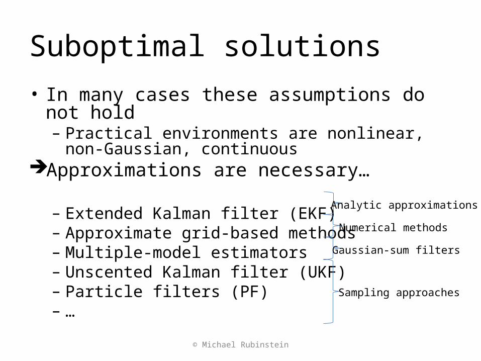
Suboptimal solutions• In many cases these assumptions do not hold
– Practical environments are nonlinear, non-Gaussian, continuous
Approximations are necessary…
– Extended Kalman filter (EKF)– Approximate grid-based methods– Multiple-model estimators– Unscented Kalman filter (UKF)– Particle filters (PF)– …
Analytic approximations
Sampling approaches
Numerical methods
Gaussian-sum filters
© Michael Rubinstein

The extended Kalman filter
• The idea: local linearization of the dynamic system might be sufficient description of the nonlinearity
• The model: nonlinear system with additive noise
),0(~),0(~
)()( 1
kk
kk
kkkk
kkkk
RNwQNv
wxhzvxfx
),RN(~w),QN(~v
wHxzvxFx
kk
kk
kkk
kkkk
00
1
© Michael Rubinstein
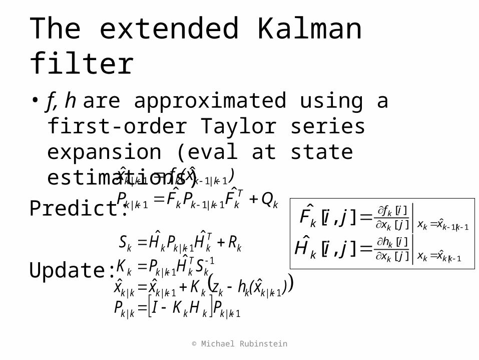
The extended Kalman filter
• f, h are approximated using a first-order Taylor series expansion (eval at state estimations)
Predict:
Update:
© Michael Rubinstein
kTk|kkkk|k
|kkkk|k
QFPFP
)x(fx
ˆˆˆˆ
111
111
1
11
11
1
ˆˆˆ
ˆ
ˆˆ
k|kkkk|k
k|kkkkk|kk|k
kTkk|kk
kTkk|kkk
PHKIP)x(hzKxx
SHPK
RHPHS1|
1|1
ˆ][][
ˆ][][
],[ˆ
],[ˆ
kkkk
k
kkkk
k
xxjxih
k
xxjxif
k
jiH
jiF

The extended Kalman filter
© Michael Rubinstein
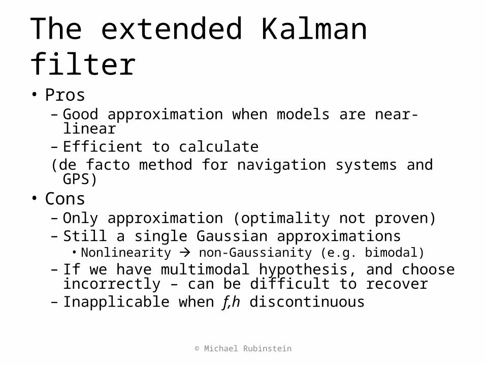
The extended Kalman filter• Pros
– Good approximation when models are near-linear– Efficient to calculate(de facto method for navigation systems and GPS)
• Cons– Only approximation (optimality not proven)– Still a single Gaussian approximations
• Nonlinearity non-Gaussianity (e.g. bimodal)– If we have multimodal hypothesis, and choose
incorrectly – can be difficult to recover– Inapplicable when f,h discontinuous
© Michael Rubinstein
Particle filtering• Family of techniques
– Condensation algorithms (MacCormick&Blake, ‘99)– Bootstrap filtering (Gordon et al., ‘93)– Particle filtering (Carpenter et al., ‘99)– Interacting particle approximations (Moral ‘98)– Survival of the fittest (Kanazawa et al., ‘95)– Sequential Monte Carlo methods (SMC,SMCM) – SIS, SIR, ASIR, RPF, ….
• Statistics introduced in 1950s. Incorporated in vision in Last decade
© Michael Rubinstein
Particle filtering
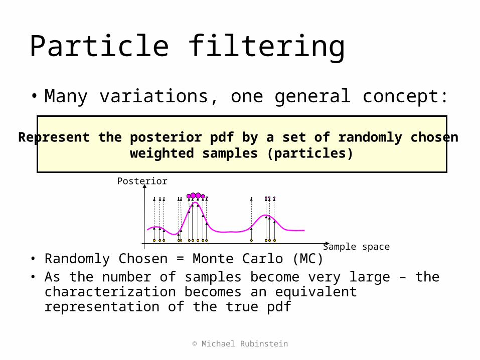
• Many variations, one general concept:
• Randomly Chosen = Monte Carlo (MC)• As the number of samples become very large – the
characterization becomes an equivalent representation of the true pdf
Represent the posterior pdf by a set of randomly chosen weighted samples (particles)
© Michael Rubinstein
Sample space
Posterior

Particle filtering
• Compared to previous methods– Can represent any arbitrary distribution
– multimodal support
– Keep track of many hypotheses as there are particles– Approximate representation of complex model
rather than exact representation of simplified model
• The basic building-block: Importance Sampling
© Michael Rubinstein