trade creation and diversion revisited: accounting for model

Trade Creation and Diversion Revisited: Accounting for Model

Uncertainty and Natural Trading Partner Effects∗

Theo S. Eicher†

University of Washington

Christian Henn

International Monetary Fund

Chris Papageorgiou

International Monetary Fund

April 20, 2010

Abstract

The effect of Preferential Trade Agreements (PTAs) on trade flows is subject to model uncertainty

stemming from the diverse and even contradictory effects suggested by the theoretical PTA literature.

The existing empirical literature has produced remarkably disparate results and the wide variety of em-

pirical approaches reflects the uncertainty about the “correct” set of explanatory variables that ought

to be included in the analysis. To account for the model uncertainty that surrounds the validity of the

competing PTA theories, we introduce Bayesian Model Averaging (BMA) to the PTA literature. Statis-

tical theory shows that BMA successfully incorporates model uncertainty in linear regression analysis by

minimizing the mean squared error, and by generating predictive distributions with optimal predictive

performance. Once model uncertainty is addressed as part of the empirical strategy, we find strong

evidence of trade creation, trade diversion, and open bloc effects. Our results are robust to a range of

alternative empirical specifications proposed by the recent PTA literature.

JEL Classification: F10, F15, C11.

Keywords: Trade Creation, Trade Diversion, Preferential Trade Agreements, Bayesian Model Averag-

ing.

∗We thank the editor and four anonymous referees for many valuable comments and suggestions. We also thank StevenYamarik for sharing his dataset and Serban Ranca for outstanding research assistance. Brian Donhauser and Alan van der Hilst

provided helpful comments. Christian Henn acknowledges support from the Henry Buechel Memorial Fellowship. The views

expressed in this study are the sole responsibility of the authors and should not be attributed to the International Monetary

Fund, its Executive Board, or its management.†Send correspondence to Theo Eicher, Department of Economics, Box 353330, University of Washington, Seattle, WA 98195

USA, email: [email protected], tel: (206) 685 8082, fax (206) 685 7477.

Trade Creation and Diversion Revisited 1

1 Introduction

Bhagwati and Panagariya (1996) call Preferential Trading Arrangements (PTAs) “two faced” because PTAs

introduce trade liberalization at the cost of discrimination. The controversy regarding the costs and benefits

of PTAs has raged since the 1950s, due to the potential for trade creation and trade diversion (Viner,

1950). Time has not provided a consensus; to the contrary, with the proliferation of PTAs in the 1990s,

the number of PTA theories that predict either increasing or decreasing trade flows among (non)members

increased in tandem. And as the number of theories expanded, the set of candidate regressors suggested

by empirical PTA research approached the point where comprehensive robustness has become virtually

unfeasible. Consequently, it has become common practice in this literature to juxtapose results that represent

alternative PTA theories. It is therefore not surprising that PTA coefficient estimates have been found to be

highly sensitive to the specific set of regressors used in any given study (see Baxter and Kouparitsas, 2006).

Ghosh and Yamarik (2004) provide the most extensive PTA robustness analysis to date. Not only do

they include a large set of PTAs, they also employ Extreme Bound Analysis (Leamer, 1983) to examine a

diverse set of PTA theories. Ghosh and Yamarik (2004) find little evidence for either trade creating or trade

diverting PTAs. They conclude that “the pervasive trade creation effect found in the literature reflects not

the information content of the data but rather the unacknowledged beliefs of the researchers.”

In this paper we apply Bayesian Model Averaging (BMA) to the PTA literature to reexamine model

uncertainty. BMA is specifically designed to incorporate model uncertainty into the estimation process, and

it is firmly rooted in statistical theory. It is a methodology that explores the model space without restrictions,

weighs each model according to quality, and provides a probability distribution for each coefficient estimate.

Raftery and Zheng (2003) prove that BMA maximizes predictive performance while minimizing the total

error rate when compared to any individual model. The rapidly growing list of economics applications using

BMA include policy evaluations (e.g. Brock, Durlauf and West, 2003), monetary policy (e.g. Levin and

Williams, 2003), macroeconomic forecasting (e.g. Garratt, Lee, Pesaran and Shin, 2003), economic growth

(e.g., Fernandez, Ley and Steel, 2001), and international economics (e.g., Chen and Rogoff, 2006).

The issue of model uncertainty surrounding PTA effects is well known in the PTA literature. Seldom

do papers present less than a dozen different PTA regression specifications. We show that BMA overturns

the fundamental Ghosh and Yamarik result by identifying a number of PTAs that exert decisive effects on

trade flows. Since Ghosh and Yamarik, the PTA literature has evolved to introduce a number of innovations

that address omitted variable bias. We show that our main finding of measurable PTA effects on trade


flows is robust, even when the Ghosh and Yamarik (2004) data set is updated to include additional years,

additional PTAs, and alternative fixed effect specifications.1 Our methodological extensions include a full

account of multilateral resistance (see, e.g., Anderson and van Wincoop, 2003; Subramanian and Wei, 2007),

bilateral unobserved heterogeneity (see, e.g., Glick and Rose, 2002; Egger and Pfaffenmayr, 2003), and an

approach to control for both multilateral resistance and heterogeneity simultaneously (Baier and Bergstrand,

2007; Baldwin and Taglioni, 2006). We also consider accession dynamics (Freund and McLaren, 1999). Our

analysis follows a voluminous literature spanned by Frankel, Stein and Wei (1995, 1997), Rose and van

Wincoop (2001), Frankel and Rose (2002), and Rose (2004).2

Our BMA benchmark specification, using Ghosh and Yamarik’s (2004) original dataset, shows strong

trade creation, trade diversion, and open bloc effects for 12 PTAs.3 Our results are at odds with Ghosh

and Yamarik (2004), even if we use their identical dataset. The differences arise for the following two

reasons: First, BMA inference is based on an unrestricted search of the model space spanned by all candidate

regressors, while Extreme Bound Analysis covers only a fraction of the model space due to the researcher’s

categorization of variables into “free” (variables that should always be included in the regression specification)

and “doubtful” (variables that may be effective in the regression specification). Second, BMA theory requires

that each model is weighed according to its posterior model probability (which is associated with the model’s

quality or performance), while Extreme Bound Analysis weighs all models equally and thus attributes the

same power of inference to both strong and exceptionally weak models.4

Even after we extend the Ghosh and Yamarik data from 1970-1995 to 1960-2000 and include more recent

bilateral trade agreements, our results remain robust. In fact, a number of PTAs are estimated with increased

precision, which allows us to identify additional trade creating PTAs. The updated dataset also modifies

the counterintuitive trade diversion effects (for NAFTA) and the unexpectedly large open bloc effects (for

MERCOSUR) that were implied by the Ghosh and Yamarik data. Controlling for multilateral resistance

does not affect our result qualitatively, and the vast majority of PTAs are shown to exert influence on trade

flows, mostly through trade creation among member countries.

1 It is important to note that most of the literature has ignored general equilibrium effects and estimates. The primary goal

of this paper is to flag more robust estimates of the “partial” or direct effects of PTAs and other controls, in order to provide

potentially better inputs for general equilibrium comparative statics.2An appealing alternative is to examine the intensive and extensive margins of trade as proposed by Helpman, Melitz and

Rubinstein (2008), and Felbermayr and Kohler (2006). We leave this to future research.3 It is common in Extreme Bound Analysis to attach all the weight of the posterior to the prior distribution. While Extreme

Bound Analysis provides no guidelines, Ghosh and Yamarik (2004) also examine the case where 95 percent of the weight of the

posterior distribution is on the prior and 5 percent on the sampling distribution — in this case they find trade creation in four

PTAs (CACM, CARICOM, MERCOSUR and APEC).4Previous comparisons between Extreme Bound Analysis and BMA results have also found Extreme Bound Analysis to be

excessively stringent (see Sala-i-Martin, 1997; and Fernandez, Ley and Steel, 2001).


Our approach to addressing multilateral resistance follows directly from Anderson and van Wincoop

(2003) and Novy (2006, 2007), as implemented by Subramanian and Wei (2007), whose context was different

and it did not address individual PTA effects. We also show that estimates based on multilateral resistance

are generally larger than estimates that account for unobserved country-pair heterogeneity (an approach

advocated by Glick and Rose, 2002; Rose, 2004; and Rose, 2005). This may be due to the methodological

difference, whereby country-pair fixed effects render estimates that measure only those PTA effects that are

directly related to accession. This raises the question of accession dynamics; we show that PTA trade effects

generally appear around accession or thereafter.5

Our most comprehensive specification controls simultaneously for multilateral resistance and unobserved

heterogeneity among countries. This specification is inspired by Baier and Bergstrand (2007), who produce a

similar specification, but without emphasis on the heterogeneous effects that individual PTAs exert on trade

flows. Even in this most comprehensive specification, we find strong effects of PTAs on trade flows, for the

Andean Pact, Central American Common Market, European Economic Area, Latin American Integration

Association, and for bilateral trade agreements.

The remainder of the paper is organized as follows. Section 2 discusses the basic framework of the BMA

methodology used in our estimation. In Section 3 we take a look at the data sets employed, and in Section

4 we report and discuss our results. Section 5 concludes.

2 The Empirical Framework

2.1 Baseline Specification

Econometric studies that seek to identify the impact of PTAs on trade flows are generally based on the gravity

model.6 The approach fits the application particularly well, due to the gravity model’s proven efficiency in

predicting trade flows (see Frankel and Romer, 1999). This allows PTA coefficients to pick up on deviations

between predicted and actual trade.

Ghosh and Yamarik (2004) include dummies that capture PTA effects on bilateral trade alongside a

matrix of other covariates, ,7 obtaining

log = + 1 log + 2 log + 3 + 4 + 5 + (1)

5The accession dynamics results are interesting in light of the emerging “endogenous PTA” strand of literature (Baier and

Bergstrand, 2007). This paper does not address endogeneity explicitly, although regressors used to control for endogeneity by

Baier and Bergstrand (2007) are included here. We discuss endogeneity bias later on. Similarly, while we are unable to prove

that our specifications are free of omitted variable bias, our expanded dataset is one of the most comprehensive to date.6The theoretical foundations of the gravity model are presented in Frankel (1997) and Deardorff (1998).7The set of specific correlates used is discussed in Section 2.3.


where average bilateral trade, , between countries and at time depends positively on national incomes,

and , and negatively on bilateral distance, . The matrix of other covariates, , is included to

represent alternative trade theories and to proxy for unobservable trade costs. The inclusion of time fixed

effects, , is standard in the literature to eliminate bias resulting from aggregate shocks to world trade, such

as global income shocks. Time fixed effects also mitigate any spurious correlation introduced, for example,

by the use of a U.S. price index to deflate all trade flows. To capture PTA effects, two sets of zero-one dummy

variables are included for each time interval, . indicates that both trading partners are members

of the same PTA in a given year, and indicates that only one member has joined. These dummies

enable us to isolate the three distinct effects that PTAs may exert on trade flows. A positive coefficient

on captures trade creation among PTA members, while trade diversion registers a negative

coefficient. Finally, open bloc trade creation is simply the opposite of trade diversion, characterized by a

positive coefficient.

2.2 Multilateral Resistance and Unobserved Heterogeneity

Equation (1) can be extended to control for multilateral resistance and unobserved country-pair heterogeneity.

In place of average trade, multilateral resistance requires the use of either bilateral imports (Subramanian

and Wei, 2007) or bilateral exports (Novy 2006, 2007) as the dependent variable.8 Here we largely follow

Subramanian and Wei (2007) to generate results that are comparable to their benchmark.

log¡Imports

¢= + + + 2 log + 3 + 4 + (2)

The added advantage of using bilateral imports, Imports, as the dependent variable is that it avoids

bias induced from averaging trade flows (see Baldwin and Taglioni, 2006).9 Since any nation faces only

one import/export price index at any point in time, multilateral resistance can be accounted for with

time-varying importer/exporter fixed effects (represented by and ).10 The inclusion of time-varying

importer/exporter effects does not allow for average trade flows as the dependent variable and we follow

Subramanian and Wei (2007) and choose bilateral imports instead. Multilateral resistance controls in (2)

absorb some of the covariates, which reduces to . Most notably the remoteness measure is now ab-

sorbed. Remoteness speaks only to GDP weighted geographic distance, which changes only slightly over time

8Some argue that this is advantageous, since trade theories yield predictions on unidirectional trade (see Freund, 2000;

Anderson and van Wincoop, 2003; Baldwin and Taglioni, 2006).9Alternative estimation approaches can also address measurement error bias see Felbermayr and Kohler (2006), and Santos

Silva and Tenreyro (2006).10Time-varying importer/exporter fixed effects are lucidly motivated by Baldwin and Taglioni (2006).


because the GDP weights are time-varying (see Section 2.3). Multilateral resistance, instead, also accounts

for variations in prices of all trading partners over time, which can imply considerable fluctuations.

In addition, multicollinearity no longer allows for the identification of separate trade creation and diver-

sion effects. In the presence of time-varying importer effects, the dummy partitions an importer’s

observations in any given year into (a) imports originating from fellow PTA members and (b) imports from

non-members. As a consequence, the dummies now expresses net trade creation, or how much

greater intra-PTA trade is compared to trade between PTA members and non-members. This implies that

when trade between members and non-members decreases because of trade diversion, the coefficient

increases in this specification.

Unobserved country pair heterogeneity can be addressed by controlling for all time-invariant bilateral

heterogeneity with country-pair fixed effects, , as follows:

log¡Imports

¢= + + 1 log + 3 + 4 + (3)

Note that now all time-invariant regressors are absorbed into the pair-specific fixed effects.11 Pair fixed

effects capture similarities of trading partners that are constant over time. With these pair-specific constants,

our regression only relies on time series variation, comparing each country pair’s observations before and

after PTA accession to determine the coefficient. Therefore here, like in equation (1),

expresses only intra-PTA trade creation. The country-pair fixed effect specification, together with Rose’s

remoteness variable to (imperfectly) capture multilateral resistance, represents a general formulation of the

gravity equation to address unobserved heterogeneity (e.g., Egger, 2000; Baldwin, 2005). If country-pair

fixed effects are omitted, the PTA coefficients tend to be biased upward because they pick up trade creation

that is not specifically PTA related, but simply due to unobservables. The introduction of country-pair fixed

effects absorbs non-time-varying control variables, which reduces the original matrix of other covariates to

(in equation 3) to (in equation 2).

The most comprehensive approach to controlling for unobserved heterogeneity, multilateral resistance,

and all other unobserved time-varying importer and exporter specific effects, is to combine (2) and (3).

This yields a specification that is most likely to generate unbiased coefficient estimates, while adhering to

theoretical foundations. This specification was suggested by Baier and Bergstrand (2007) in the context of

estimating average trade effects across all PTA member countries. It can be obtained by adding country-pair

11We estimate equations (2-4) using the Andrews, Schank and Upward’s (2006) “FEiLSDVj” estimator, which relies on

partitioned regression techniques to reduce computational burden; it delivers identical results to LSDV regressions.


() fixed effects along with the time-varying importer/exporter (, ) fixed effects to equation (1).12

log¡Imports

¢= + + + 2 log + 3 + 4 + (4)

Baier and Bergstrand (2007) also point out that in panel data, fixed effects or first differencing can be

employed to address some of the potential endogeneity in the PTA regressions.13 The fixed effects in equations

(2)-(4) can partially address two out of three sources of endogeneity bias. The first type of endogeneity bias

may arise in equation (1) between GDP and trade flows (see Frankel and Romer, 1999). The inclusion of

time-varying importer/exporter fixed effects will contain this source of bias. The second type of bias arises

due to the endogeneity between trade flows and trade policies. Trefler (1993) first used instruments to addess

the endogeneity of trade policies and found the effect of such policies to increase tenfold. Lee and Swagel

(1997) also document that the effect of trade liberalization on imports is biased downward in the absence of

instrumenting for endogeneity.

The third source of possible endogeneity is that countries might endogenous select into (specific) PTAs.

This bias is less likely addressed by fixed effects. Baier and Bergstrand (2004a) find cross-section evidence

that country pairs with common economic characteristics also tend to share PTA memberships. Baier and

Bergstrand (2007) suggest that the endogeneity of PTA membership likely renders the PTA coefficient biased

downward in cross sections.14 They argue that a key source of this endogeneity may be bilateral unobserved

characteristics, for example, common institutions or regulations. Such unobserved bilateral characteristics

may be the determinants of countries’ trade and of their PTA membership decisions. In this case the

endogeneity bias would be largely cross-sectional in nature, and it can be controlled by the country-pair

fixed effects that we include in our panel regressions.

Egger (2004) argues that the estimates obtained in the regressions above may be biased downward if

there exist cross section dependencies that result in correlations between explanatory variables and unob-

served bilateral effects exists. Thus he proposes the Hausman and Taylor (1981) Two Stage Least Squares

12The alternative would be to first-difference. Wooldridge (2002, Chapter 10) shows that when the number of time periods

exceeds two, the fixed-effects estimator is more efficient under the assumption of serially uncorrelated error terms. Baier and

Bergstrand (2007) provide a comprehensive discussion of the two approaches whose results might differ slightly depending on

the length of the panel and the structure of the error terms. Although both approaches have advantages and disadvantages,

Baier and Bergstrand show in a panel that is basically identical in error structure to ours, that the results are very similar.

Hence we present the fixed effects results below.13Aside from Baier and Bergstrand (2007), the potential PTA endogeneity bias in cross-section gravity models is also addressed

by Baier and Bergstrand (2002, 2004b) and Magee (2003), but with mixed success. Baier and Bergstrand (2007) also lament

that “... other methods to identify the impact, such as instrumental variables using cross-section data, are compromised by a

lack of suitable instruments.”14To paraphrase, their reasoning is that PTA membership of a trading pair and the intensity of their domestic regulations

may be positively correlated in a cross-section of data, but the gravity equation’s error term and the intensity of domestic

regulations may be negatively correlated. Hence the PTA dummies and the error term are negatively correlated, and the

PTA coefficient will tend to be underestimated.


Error Components model. Serlenga and Shin (2007) incorporate the Egger methodology into the correlated

common effect pooled (CCEP) estimation approach, which was advanced by Pesaran (2006). Serlenga and

Shin (2007) highlight that the bias can go either way, depending on the specific coefficient estimate and time

period examined. This is not surprising since the exact bias depends on the specific correlation structure.

Unfortunately, the methods developed by Hausman and Taylor (1981), Pesaran (2006), and Serlenga and

Shin (2007) are not available for Bayesian Model Averaging. Thankfully, however, this type of bias is not of

crucial importance in our application since we focus primarily on the coefficients of the time-varying PTA

dummies (which are still estimated consistently) and not on the magnitude of time-invariant regressors (such

as distance).

Serlenga and Shin (2007) further show that the gravity equation may be biased due to possible cross-

section dependence arising from unobserved (heterogeneous) time-specific factors. The authors thus adopt

an alternative estimator, originally proposed by Pesaran (2006), to explicitly address such dependencies. The

Pesaran estimator has not been implemented in a BMA context, hence we limit ourselves to the approaches

that we introduced above. While we are mindful of this bias, we nevertheless regard it as important to

consider results that have been obtained via a principled approach to model uncertainty. If anything, the

previous literature seems to suggest that the derived estimates are generally too low.

Another bias may arise due to spatial heterogeneity (structural instability or heteroskedasticity, see

Anselin and Griffith, 1988). This may lead to biased parameter estimates or misleading significance levels.

Bougheas, Demetriades, and Morgenroth (2003) explore the spatially autocorrelated error terms and use

instrumental variables in an attempt to address the issue. Their results show the bias can go either way,

depending on the application. Baltagi, Egger and Pfaffermayer (2007) also highlight the importance of spatial

autoregressive error processes that apply to both the individual and remainder error components. They

suggest a maximum likelihood estimator for a general spatial panel with random effects. Here we presume,

consistent with previous literature, that the fixed effects model is predominant for our trade application.

2.3 Model Uncertainty in PTA Theory

A voluminous theoretical literature discusses appropriate controls in gravity models, which include proxies

for geography, history, economic policy, and development and factor endowments. Each control is motivated

by a particular theory. At times the same control is claimed for different theories (with the opposite sign),

underlining the rampant model uncertainty. Below we provide a brief description of the theoretical under-

pinnings of the various controls suggested by the previous literature. It is crucial to outline this diversity of


approaches to justify the use of the model averaging methodology.

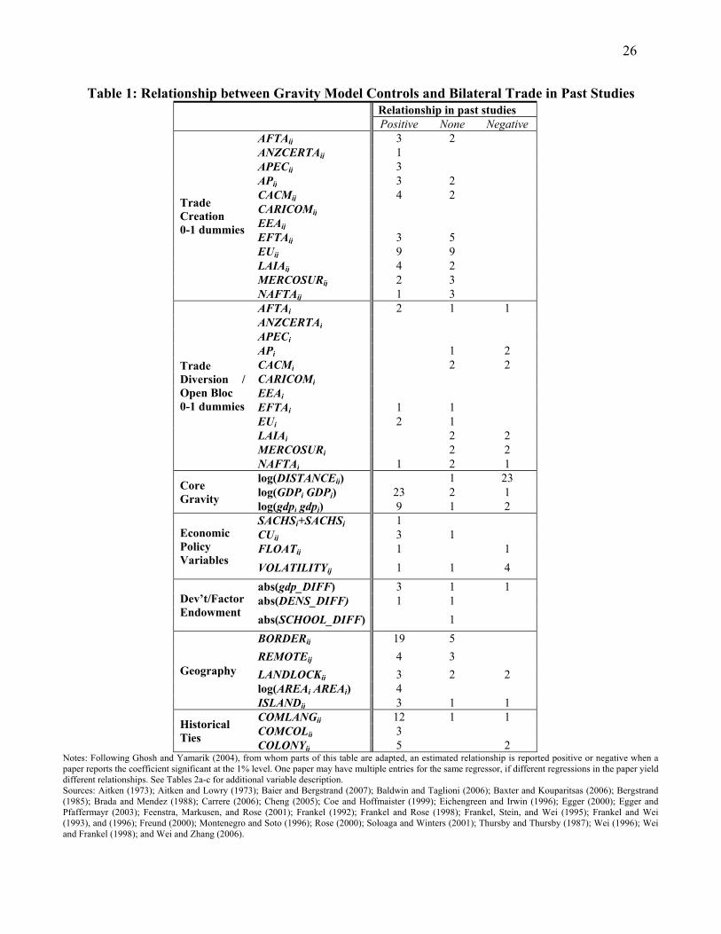
Table 1 summarizes the extend of the model uncertainty by tabulating the covariates suggested by earlier

studies. It highlights the numerous attempts to identify determinants of trade flows and the associated

diversity of results. The table shows how important it is to incorportate the model uncertainty that is

inherent in gravity/PTA regressions as part of the empirical strategy. When the uncertainty about the true

specification is not accounted for in the econometric method, the precision of estimates is inflated, since they

neglect the uncertainty surrounding the true theory.

It is important to outline the theoretical backbone for each covariate included in the analysis. Without

theoretical support, the results are difficult to interpret. The first set of control variables captures historical

ties, such as Common Language, Common Colonizer, or Colony. These covariates are commonly included to

capture transaction costs due to communication and/or cultural differences.15 Common historical ties lead

to similar institutions and similar levels of development, implying reliable contractual and legal standards,

as well as trust in shared values. Controlling for model uncertainty addresses not only which one of these

regressors (or regressor combinations) is appropriate, but also whether their inclusion is indeed approximating

the true model.

Geographic factors have been introduced as proxies for transport costs (e.g., Aitken, 1973), trade-and-

geography theories (e.g., Helpman and Krugman, 1985), or New Trade Theories (e.g., Rivera-Batiz and

Romer, 1991). Remoteness (developed by Rose, 2000) is the GDP-weighted negative of distance that is

often included to capture the notion that relatively remote country pairs are expected to trade more, because

they have fewer options in choosing trade partners.16 It has also been motivated as a proxy for multilateral

resistance, or the average trade costs facing a country (Carrere, 2006). Land Area is intended to capture

self-sufficiency and scale effects that are prominent in both the new trade and growth theories (e.g., Rose,

2000; Rose and Van Wincoop, 2001). Scale effects are also proxies for technology or knowledge spillovers

(e.g., Grossman and Helpman, 1991).

Alternative proxies in the geography category, such as Border, Landlocked, and Island have previously

been utilized by a variety of authors, although it is not immediately clear why adjacency should matter after

having controlled for distance.17 Perhaps variables that measure distance center-to-center introduce errors

that are mitigated by the additional controls, because neighboring countries often engage in large volumes of

15See Wei (1996), Frankel (1997), Rose (2000), Soloaga and Winters (2001), Rose and van Wincoop (2001), and Frankel and

Rose (2002).16 See Wei (1996), Rose (2000), Soloaga and Winters (2001), and Baier and Bergstrand (2007).17 See Frankel and Romer (1999), Rose (2000), Feenstra, Markusen and Rose (2001), Rose and van Wincoop (2001), Soloaga

and Winters (2001), and Frankel and Rose (2002).


trade. BMA addresses the uncertainty surrounding the inclusion of geography variables by indicating which

covariates are relevant to explaining how PTAs influence trade patterns.

Covariates for development and factor endowments juxtapose the Heckscher-Ohlin factor endowments

trade theory with Linder’s (1961) hypothesis, which holds that similar countries should trade more because

of their similar tastes. Davis (1995) presents an augmented Heckscher-Ohlin-Ricardo model that provides

support for either theory, depending on the technological distance between the countries, and Spilimbergo

and Stein (1998) examine the issue empirically. Common proxies for factor endowment differences are based

on Per Capita GDP, Schooling, and Population Density.18 The theoretical rationale for Per Capita GDP

is based on the strategic trade literature (e.g., Helpman and Krugman, 1985), which predicts intra-industry

trade to increase as countries become more similar in their levels of development. Furthermore, countries

with higher per capita GDP are likely to have better access to less distortionary revenue sources. Hence they

may experience more bilateral trade since they can afford lower tariffs.

Economic policy variables that are commonly included relate to trade/financial openness and exchange

rate management. These are important controls as trade restrictions can explain deviations from trade

patterns implied by the pure gravity equation. The Sachs and Warner (1995) Trade Openness variable

is inserted into the gravity equation to account for trade policy effects. In addition, proxies that measure

capital account openness, and financial transaction costs such as Currency Union, Floating FX Rate, and FX

Volatility are usually included although it is not clear what coefficient estimates are to be expected. Clark

et al. (2004) survey the literature and highlight that just this subset of regressors alone is so deeply affected

by model uncertainty that the impact of exchange rate fluctuations depends on the specific assumptions of

each model.19

Finally we address model uncertainty in the PTA theory itself.20 Not only do we have opposing implica-

tions suggested by different theories, but at times opposing theories have been suggested by the same author

(see, e.g., Krugman, 1991a,b). The theory of PTAs is based on Viner’s (1950) theory of trade creation and

diversion. By the 1990s, a full-scale discussion erupted regarding the drivers of trade creation and diversion.

Krugman (1991a,b) examined the relative merits of PTAs in a static, monopolistically competitive frame-

work that emphasized economic geography. His first model implied PTAs should not be welfare creating in

the absence of intercontinental transport costs. At the other extreme, Krugman’s second model suggested

18They have been introduced by Frankel (1992), Frankel and Wei (1993), Frankel, Stein and Wei (1995), Frankel (1997),

Freund (2000), Rose and van Wincoop (2001), and Frankel and Rose (2002).19Authors who introduced such regressors into the gravity equation include Rose (2000), Frankel and Rose (2002), Rose and

van Wincoop (2001), Glick and Rose (2002), and Tenreyro and Barro (2007).20For a more detailed literature review, see Panagariya (1999, 2000).


regional PTAs increase trade flows and subsequently welfare in the presence of prohibitive inter-continental

transport costs.

Krugman’s theories led Frankel, Stein, and Wei (1995), Frankel (1997), and Wei and Frankel (1998)

to develop theories based on a continuum of transport costs. Their work characterizes trade partners as

“natural” on the basis of relatively low intercontinental transport costs and their approach implies that trade

creation among “natural” trading partners should dominate small trade diversion among remote country pairs

from a welfare perspective. As trade costs fall, however, trade diversion may become larger since “natural”

trading partners overly skew their trade toward PTA partners. Frankel, Stein and Wei (1995) suggest two

hypotheses. First, the more remote trading partners are from the rest of the world, the more likely they are

to form PTAs due to less potential trade diversion. This effect could be picked up by the Remoteness proxy.

Second, the more “natural” trading partners are, the more likely PTAs are to lead to trade creation.

Krugman’s and Frankel, Stein and Wei’s theories are based on one factor/one industry models. Deardorff

and Stern (1994) note that these models preclude trade due to comparative advantage. Deardorff and

Stern point out that this “stacks the deck” against bilateralism and argue that, given differences in factor

endowments, trade with a few countries suffices in order to maximize gains from trade. Thus trade diversion

would be minimal. In response, Baier and Bergstrand (2004) construct a model that builds upon Frankel,

Stein and Wei (1995) to allow for comparative advantage and scale effects. Freund (2000) argues strongly

for PTA open bloc trade creation effects (even if trade creation among members is absent) since PTAs help

outside exporters overcome fixed trade costs. Trade diverting effects, instead, are highlighted by Bond and

Syropoulos (1996), who indicate that the increased market power of PTAs, relative to the market power of

each member taken individually, may lead to higher external tariffs.

2.4 Bayesian Model Averaging

This section briefly outlines the BMA methodology used in the estimation. We limit ourselves to discussing

the properties relevant to our application. The interested reader is referred to the comprehensive tutorial by

Raftery, Madigan and Hoeting (1997) for further discussion.21 BMA is a natural candidate to address model

uncertainty surrounding the correct controls in equations (1)-(4), since it provides probability distributions

over both the model space and the parameter space. In our PTA estimation, the model space consists of all

the possible subsets of candidate regressors that have been suggested by the distinct theories summarized

above.

21For recent methodological contributions to BMA see e.g. Doppelhofer and Weeks (2009), Ley and Steel (2009), and Eicher,

Papageorgiou and Raftery (forthcoming).


For linear regression models, the basic BMA setup can be concisely summarized as follows. Given a

dependent variable, Y, a number of observations, n, and a set of candidate regressors, 12 , the

variable selection problem is to assess the quality of model

= +

X=1

+ (5)

where 12 is a subset of 12 , and is a vector of regression coefficients to be estimated.

Note that (5) is specified for linear models. Given the data, , BMA first estimates a posterior distribution

(| ) for every candidate regressor, , in every model that includes . It then combines all

posterior distributions into a weighted averaged posterior distribution, (|) , using each model’s posteriorprobability, (|), as model weight

(|) =X∈

(| ) (|) (6)

The posterior model probability of is simply the ratio of its marginal likelihood to the sum of the

marginal likelihoods over all other models

(|) = (|)

2P=1

(|)

(7)

where posterior model probabilities are also the weights used to establish the posterior means and variances

≡ [|] =X

∈ (|) (8)

≡ [|] =X

∈

³ [|] +

2

´ (|)− [|]2 (9)

Summing the posterior model probabilities over all models that include a candidate regressor, we obtain the

posterior inclusion probability

( 6= 0|) =X∈

(|) (10)

The posterior inclusion probability provides a probability statement regarding the importance of a re-

gressor that directly addresses the researchers’ prime concern: What is the probability that the regressor

has a non-zero relationship with the dependent variable? The general rule developed by Jeffries (1961) and

refined by Kass and Raftery (1995) stipulates effect-thresholds for posterior probability. Posterior probabil-

ities 50% are seen as evidence against an effect, while the evidence for an effect is either weak, positive,

strong, or decisive for posterior probabilities ranging from 50-75%, 75-95%, 95-99%, and 99%, respectively.

In our analysis, we refer to a regressor as “effective,” if its posterior inclusion probability exceeds 50%.


BMA has a number of key advantages over estimating a single model, and over Extreme Bound Analysis.

Raftery and Zheng (2003) show that BMA a) minimizes the total error rate (sum of Type I and Type

II error probabilities), b) its point estimates and predictions minimize mean squared error (MSE), and c)

its predictive distributions have optimal predictive performance relative to other approaches. Contrary to

Extreme Bound Analysis, BMA examines the entire model space and imposes no restrictions on the model

size. Ghosh and Yamarik (2004) only consider models that contain a specific number of fixed variables. In

addition to these fixed regressors, a fixed number of regressors is rotated in and out of ech regression. This

approach limits the model search to a fraction of the model space that is spanned by all candidate regressors.

This has been shown to render Extreme Bound Analysis excessively stringent (see Sala-i-Martin, 1997).

3 Data

Our dataset is based on the Ghosh and Yamarik (2004) dataset to allow for a direct reexamination of their

evidence using BMA as our alternative statistical methodology. The Ghosh and Yamarik dataset is based on

Frankel and Rose (2002) and it includes 12 PTAs,22 3,420 bilateral trade pairs at five year intervals from 1970

to 1995, and a total of 14,522 observations.23 This dataset features average bilateral trade as the dependent

variable, recorded in U.S. dollars and deflated by the U.S. GDP chained price index. In addition to the

basic gravity and trade agreement variables, 16 control variables have been suggested by various gravity

approaches discussed above.

To address refinements in the theoretical and empirical trade flow specifications suggested by the recent

literature, we expand the baseline dataset in several dimensions. We extend the time horizon from 1960

to 2000 and allow for 60 additional (bilateral) trade agreements that are included in the Subramanian

and Wei (2007) dataset, which features 164 importers and 177 exporters. This increases the total number

of observations to 37,983.24 We follow Subramanian and Wei (2007) and choose bilateral imports as the

dependent variable; nominal imports are obtained from the IMF’s Direction of Trade Statistics.25 Overall

our updated dataset extends the unbalanced panel of Subramanian and Wei (2007) in the following three

22The PTAs are the European Union (EU), European Free Trade Arrangement (EFTA), European Economic Area (EEA),

Central American Common Market (CACM), Caribbean Community (CARICOM), North American Free Trade Agreement

(NAFTA), Latin American Integration Association (LAIA), Andean Pact (AP), Southern Cone Common Market (MER-

COSUR), Association of South-East Asian Nations Free Trade Area (AFTA), Australia-New Zealand Trade Agreement

(ANZCERTA), and Asian Pacific Economic Cooperation (APEC).23 See Ghosh and Yamarik (2004, Appendix C) for further details.24With 177 countries in the IMF’s Direction of Trade Statistics, as obtained by Subramanian and Wei (2007), potentially

trading in the 9 time periods from 1960-2000, we have 177 ∗ 176 ∗ 9 = 280 368 potential observations. Of these, 72,211 report

non-zero values. Dropping observations with import values of less than $500,000, reduces the dataset to 52,340. Missing values

for key covariates reduce the dataset by another 14,357 observations to yield our final dataset of 37,983 observations.25Note that Subramanian and Wei (2007) deflate bilateral imports by the U.S. CPI. Here we use nominal import values as

they yield the same results once time fixed effects are included (see Baldwin and Taglioni, 2006).


dimensions: (a) it disaggregates the Subramanian-Wei catch-all PTA variable, (b) it allows for additional

PTAs not considered in Subramanian and Wei (2007),26 and (c) it incorporates a comprehensive list of

additional controls suggested by the previous literature. Detailed descriptions of the PTAs and the other

control variables included in the extended dataset can be found in Tables 2a-c.

The Subramanian and Wei (2007) data is in turn based on Rose’s (2002, 2004) work on the determinants

of trade flows; we maintain their convention of including only those of the roughly 280,000 observations whose

trade values exceed $500,000. There exists, however, an important literature that seeks to understand the

true nature of the data when zero trade flows are observed. Zero trade values may also be due to a rounding

error or missing observations, and in a log linear gravity equation zeros are automatically excluded. If a zero

trade value were to be an accurate representation of two countries’ goods trade, the observation should not

be excluded, since it holds information and its absence may induce selection bias.

Santos Silva and Tenreyro (2007) suggest the Poisson pseudo-maximum-likelihood (PPML) estimator to

appropriately address the issue of zero trade values. This method has been shown to reduce estimates by

as much as 40 percent. Martin and Pham (2008) suggest that the PPML estimator is efficient in addressing

heterogeneity, but still biased in the presence of zero trade values. Based on the results of their simulations,

they instead recommend a Heckman Maximum Likelihood approach to control for selection bias. Below

we follow Rose’s and Subramanian and Wei’s OLS approach not only to maintain comparability with their

results, but also because neither a PPML nor a Heckman estimator has been developed to date for BMA

application.

4 Results

4.1 PTA Trade Creation: Differences due to Methodologies

Ghosh and Yamarik (2004) embarked on the most comprehensive robustness test of PTAs to date. They

considered not just a subset, but all major PTAs and employed Extreme Bound Analysis to explore the

model space far beyond what ordinary robustness exercises can hope to represent. Our first objective is

to replicate Ghosh and Yamarik’s (2004) results using BMA methodology. Table 3 reports results for two

specifications. Specification 1 employs BMA on the exact same data and regression equation in Ghosh and

Yamarik (2004, equation 1). Specification 2 differs from Specification 1 only in that it uses our new updated

dataset based on Subramanian and Wei (2007).

26This extension adds the European Free Trade Agreement (EFTA), the European Economic Area (EEA), the Andean Pact

(AP), the Latin American Integration Associationand the Asia Pacific Economic Community (APEC) to the analysis.


Table 3 highlights that our key result is independent of the choice of PTA data set that is used. Once

model uncertainty is addressed in a principled fashion using BMA, Ghosh and Yamarik’s (2004) own econo-

metric specification produces a host of PTA effects that range from trade creating to open bloc and even

trade diverting. We obtain effective coefficients (indicated with asterisks) whose signs and magnitudes are

similar to those commonly reported in the previous literature. BMA thus provides evidence that the model

space spanned by “free and doubtful variables” through Extreme Bound Analysis was too restrictive. The

models flagged out by Extreme Bound Analysis did not contain those that feature the highest posterior

probabilities, and the heuristic model weighting assigned by Extreme Bound Analysis generated excessively

conservative results that indicated no PTA effects. The expanded model space, combined with the principled

weighting of effective models, generate BMA’s superior predictive performance.

Of the 13 major trade agreements, 8 are found to be either trade creating and/or to exhibit open bloc

effects in Specification 1. All western hemisphere PTAs are identified as trade diverting in the original Ghosh

and Yamarik dataset (Specification 1). The additional years and controls for bilateral agreements in our

updated dataset (Specification 2) increase the precision of the estimates, but our key insights remain the

same. Specification 2 produces four additional trade creation effects (for key PTAs such as the EFTA, AFTA

and the EU), and erases the odd implication of NAFTA trade diversion that was reported by Specification

1. These changes are most certainly due to the extension of the time horizon from the mid 1990s to 2000.

In summary, the BMA results robustly link PTAs to changes in trade flows, although the effects vary across

PTAs.

A substantial literature addresses the possibility of PTA coefficient bias due to omitted variables or

inaccurate model specification. We extend our analysis to incorporate the insights of this recent literature to

examine the robustness of our results. The scale of some PTA coefficients in Table 3 is certainly suspicious

if not implausible. Coefficients that exceed unity imply that a PTA increased trade more than twofold

(since the regression is in logs). Such aberrant magnitudes have previously been noted and questioned in the

literature (e.g., Frankel, 1992; Frankel and Wei, 1993; Frankel, Stein and Wei, 1995; Frankel, 1997). We take

up the issue of omitted variable bias in the following section.

4.2 Multilateral Resistance

Ghosh and Yamarik (2004) and our Specifications 1 and 2 (Table 3) include time fixed effects, but the recent

PTA literature suggests the inclusion of additional fixed effects to account for multilateral trade costs. Wei

(1996), Deardorff (1998), Anderson and van Wincoop (2003), and Subramanian and Wei (2007) emphasized


that the standard gravity model is subject to misspecification bias if multilateral trade costs are ignored. The

crucial insight is that bilateral trade is influenced by the average multilateral trade cost faced by a country

in any given period. Anderson and van Wincoop (2003) suggest that, empirically, the inclusion of country

fixed effects captures multilateral resistance. Since bilateral trade between any two countries depends on

the multilateral resistance of both importers and exporters, the Anderson and van Wincoop (2003) model

requires fixed effects for both countries involved in any bilateral trading relationship.27 In a panel, these

importer and exporter fixed effects must be time varying, which allows the PTA dummies in equation (2) to

identify net trade creation. This fixed effect approach has been popularized by Subramanian and Wei (2007)

in their analysis of WTO trade effects (although these authors do not break out the effects of individual

PTAs).

Specification 4 reports results that control for multilateral resistance. Specification 3 replicates the results

in Specification 2, without separate trade diversion/open bloc effects. As expected, the results for most trade

agreements are very similar to the sum of trade creation and diversion in Specification 2. For example, the

Central American Common Market (CACM) featured a coefficient for trade creation of 2.3 in Specification

2, and a trade diversion effect with the rest of the world of 0.17. The combined net trade creation for PTA

members is then an implied 2.47, which is closely matched by the estimate of 2.45 in Specification 3.

More importantly, however, Table 4 shows that even after controlling for multilateral resistance, the

fundamental result of our analysis remains unchanged: PTAs have a strong impact on bilateral trade. Of

the 13 major PTAs covered, 10 PTAs exhibit an effect on bilateral trade, only one of which is negative. This

implies that controlling for multilateral resistance identifies four additional PTAs with significant positive

impacts on bilateral trade flows.

The one surprise in Specification 4 is the implied negative net trade creation for the EU. The attractiveness

of the EU market with its large size and strong harmonization likely exerts a significant pull on non-EU

exporters, resulting in the large open bloc effects estimated at about 0.6 in Specifications 1 and 2. The

drag of open bloc effects on net trade creation by itself thus explains roughly half of the negative coefficient

estimate. In addition, it is well known that the gravity equation overpredicts EU trade when estimated on

a global sample. Given their close proximity and other bilateral characteristics, EU countries undertrade

relative to the globally-based prediction, resulting in a negative EU coefficient. This may be related to the

gravity equation’s inability to proxy firms’ fixed costs in establishing trade relations (e.g. Freund, 2000).

27Helpman, Melitz and Rubinstein (2008) suggest an alternative rationale for importer and exporter fixed effects based on

firm heterogeneity.


Empirically, Aitken (1973), and Rose (2004) find similarly negative EU results. Inclusion of country-pair

fixed effects is commonly suggested to control for such time-invariant bilateral heterogeneity. It represents the

main alternative to time-varying importer/exporter fixed effects for our robustness analysis. By examining

EEA, EFTA and EU effects across alternative fixed effects specifications, Baier, Bergstrand, Egger, and

McLaughlin (2008) also find a similar instability and turn to country-pair fixed effects to obtain robust

effects.

4.3 Unobserved Heterogeneity

To capture unobserved time-invariant heterogeneity among trade partners, we reestimate Specification 4,

accounting for country-pair fixed effects. This specification does not address multilateral trade costs as com-

prehensively as suggested by Anderson and van Wincoop (2003), especially if they exhibit large fluctuations

over time. However, Rose (2004) makes the point that country-pair fixed effects constitute a valid proxy for

average multilateral resistance exhibited in country pairs. Hummels and Levinsohn (1995) first introduced

country-pair fixed effects to better distinguish between factor endowments and market structure as trade

flow drivers. Egger and Pfaffermayr (2003) advocate country-pair fixed effects to account for heterogene-

ity induced by time-invariant factors (e.g., geography, history, policy, and culture) that are only partially

accounted for by the explanatory variables or completely unobserved. Glick and Rose (2002) use the same

specification as Egger and Pfaffermayr (2003), but motivate country-pair fixed effects as proxies for trade

resistance. Here we employ it as a robustness test of the estimated parameter magnitudes for specific PTAs,

such as the EU.

Note that the introduction of country-pair fixed effects removes the cross-sectional information so that

Specification 5 relies only on the time-series information contained in the data. Specification 5, therefore,

expresses only PTA effects directly caused by PTA accession or exit. Nevertheless, our central result remains

robust: PTAs exert a significant effect on trade flows. The rewarding aspect of the country-pair analysis

is that BMA confirms the hypothesis that the gravity model overpredicts intra-European trade flows only

when pair specific heterogeneity is ignored. Once these effects are accounted for, EU trade creation is

indeed positive. On the other hand, some effects that seemed unreasonably large before are now significantly

reduced. ANZCERTA, AP, EEA and MERCOSUR lose their influence on net trade flows, which indicates

considerable unobserved bilateral heterogeneity members of these PTAs. With the exception of the Latin

American Integration Association (LAIA), magnitudes of significant PTA impacts are uniformly smaller

when we explore only the specific effect of entering and exiting a trade agreement.


4.4 A Comprehensive Approach

The previous sections illustrated how each individual fixed effect approach influences PTA estimates. In

this section we present results from our most comprehensive approach, which controls for both unobserved

heterogeneity and multilateral resistance simultaneously. The comprehensive approach adds a large number

of fixed effects controls to the regression, and is identical to the Baier and Bergstrand (2007) methodology.

However their focus was on the average PTA effect, while the motivation for this paper was to show the

heterogeneity of trade effects across individual PTAs and to resolve model uncertainty. As outlined above,

the comprehensive approach is also best suited to control for the various biases may be contained in a gravity

equation, especially endogeneity bias.

Specification 6 in Table 4 presents new results and present a number of additional insights. Even after

accounting for the large number of fixed effects, and after accounting for model uncertainty, a series of

PTAs show strong effects on trade flows. CACM, CARICOM, EEA and LAIA all exhibit high inclusion

probabilities and positive trade effects. The EU which oscillated from negative to positive coefficients is now

economically significant but only marginally statistically significant. Note, however, that the EEA picks up

important recent trade effects among a large number of EU members. We also find a dramatic reduction

in predicted trade flows due to a PTA among the APEC countries. This is comforting since APEC did not

institute actual tariff reductions, and it has been well known that the gravity models must have attributed

some of the bilateral or individual country effects to the creation of APEC. Once we control for these effects,

and for the potential endogenous selection of fast trade-growing countries into AFTA, we find that the actual

affect of APEC is nil.

Among the non-PTA variables, only the difference in GDP remains significant. The coefficient indicates

that countries with similar GDP generate larger trade volumes, which supports intra-industry trade theories

rather than Heckscher-Ohlin. The variation of the results across different fixed effects raises the general

question of integration dynamics. Are average estimates over the life of PTA membership appropriate, or

can we observe accession dynamics where static effects (before or at accession) differ fundamentally from

subsequent dynamic changes in trade flows? If we are interested in the specific effects of individual trade

flows, there may well be accession dynamics in play that suggest that the simple averaging of effects over

time may be misleading. We examine this hypothesis in the following section.


4.5 Accession Dynamics

Further investigation of accession dynamics may also yield benefits beyond the reconciliation of remaining

differences between Specifications 4 and 5. Namely, accession dynamics provide insights whether gains from

trade tend to be static, as advocated by neoclassical trade theory, or dynamic (e.g., Young 1991). Indeed the

gain might even commence before the PTA accession. Hence we recode the PTA dummy into three separate

effects. If accession occurs at time t, an accession dummy captures trade creation when the country joined

a PTA, a pre-accession dummy captures the 5 years prior to joining a PTA (t-1 in our notation), and a

post-accession dummy captures the 5 years following accession to the end of the sample, (t+1, n), where n

indicates either the year 2000 or the year a country exited the PTA.

Results that include accession dynamics are presented in Table 5, where we present specifications that

control for multilateral resistance (Specification 4a), unobserved bilateral heterogeneity (Specification 5a),

and for both of the former (Specification 6a). For expositional purposes, Table 5 does not report non-

PTA regressorsw that were included in the analysis to save space. The posterior estimates and inclusion

probabilities are very similar to the corresponding specifications without accession dynamics. Table 5 also

includes the average PTA effects (t, n) established in Specifications 4-6 to allow for quick comparisons

between average effects and accession dynamics for each PTA.

The accession dynamics highlight the timing of the trade gains for each PTA. In general, the PTAs’

effects on trade materialize in the accession and post-accession phases with the appropriate magnitudes.

The accession results also show a high coincidence between average effects and dynamic effects; namely only

PTAs that produce average effects in Table 4 also produce dynamic PTA effects in Table 5. There are

two interesting exceptions to this rule. In specification 6, where we control for both country-pair and time-

varying importer/exporter time fixed effects, we find that there is a gradual onset of trade creation for those

PTAs with overall net trade creation. The Latin America Integration Association (LAIA) and the European

Economic Area (EEA) illustrate that net trade creation first becomes notable in the accession period and

fortifies thereafter. The patterns in the Central American Common Market (CACM) and bilateral trade

agreements differ slightly. These PTAs show negative net trade creation pre-accession, which is remedied

by accession to the PTA. PTA accession thus created trade, correcting for members’ previously observed

undertrade relative to the gravity prediction.


4.6 Other Determinants of Trade Flows

So far we have discussed only the impact of PTAs on trade flows. However, the BMA exercise holds important

additional information regarding other determinants of trade flows. The geography and history controls are

highly significant in Specifications 1 and 2 (in agreement with the previous literature). Althought the

magnitues of their effects are reduced by the fixed effects, they generally remain significant.

BMA identifies trade openness as a key variable in all specifications, which is not surprising since we

are attempting to explain trade flows. More interesting is that a number of variables related to exchange

rate policy are not significant unless we control for bilateral unobservables. The currency union variable,

on the other hand, shows a strong effect independent of dataset or empirical specification. Additional

variables that might influence trade flows are factor endowments. Here BMA allows us to examine the

competing hypotheses that trade flows are either driven by differences in endowments (Heckscher-Ohlin)

or by similarities (Lindner). In Specifications 1 and 2, the Heckscher-Ohlin factor endowment theory finds

strong support as differences in per capita GDPs and population densities are strongly associated with greater

trade flows. The endowment effect vanishes, however, when we consider multilateral resistance. Effects of

population density disappear once we account for bilateral heterogeneity. Finally, the BMA methodology

shows that differences in schooling increase bilateral trade flows when we control for either unobserved

heterogeneity or multilateral resistance.

5 Conclusion

The literature on preferential trade agreements (PTAs) features an unusual diversity of theoretical and

empirical approaches. In this paper we incorporate model uncertainty into the empirical strategy by applying

Bayesian Model Averaging (BMA). To date the most extensive robustness analysis by Ghosh and Yamarik

(2004) used Extreme Bound Analysis and found evidence against any effects of PTAs at the extreme bounds.

In contrast, applying BMA to Ghosh and Yamark’s original dataset we find that PTA trade creation is strong.

In addition, the BMA approach produces coefficient estimates that resolve a number of empirical puzzles.

We confirm strong PTA effects not only with Ghosh and Yamarik’s original dataset, but also with

an updated dataset that includes additional years and PTAs. Our results are robust to the inclusion of

multilateral resistance, accession dynamics, and unobserved bilateral heterogeneity. Overall, the observed

PTA effects reflect the diversity of PTAs and the degree of tariff reductions they encompass. BMA allows

us to also account for model uncertainty in the set of additional control variables usually featured in PTA


regressions. Our approach highlights the importance of including all controls for policy, development, factor

endowments, geography, and history that have been suggested by the previous literature. Among these

regressors, the only ones that receive mixed evidence are those related to exchange rate fluctuations.


6 References

Aitken, N.D., 1973. “The Effect of the EEC and EFTA on European Trade: A Temporal Cross-SectionAnalysis,” American Economic Review, 63, pp. 881-892.

Anderson, J., van Wincoop, E., 2003. “Gravity with Gravitas: A Solution to the Border Puzzle”, AmericanEconomic Review, 93, pp. 170-192.

Andrews, M., Schank, T., Upward, R., 2006. “Practical Fixed Effects Estimation Methods for the Three-Way Error Components Model,” The Stata Journal, 6, pp. 461-481.

Anselin, L. and Griffith, D.A., 1988. “Do Spatial Effects Really Matter in Regression Analysis?” Papers,Regional Science Association, 65, pp. 11-34.

Baier, S.L., Bergstrand, J.H., 2002. “On the Endogeneity of International Trade Flows and Free TradeAgreements,” Manuscript, University of Notre Dame.

Baier, S.L., Bergstrand, J.H., 2004a. “Do Free Trade Agreements Actually Increase Members’ InternationalTrade?” Manuscript, University of Notre Dame.

Baier, S.L., Bergstrand, J.H., 2004b. “Economic Determinants of Free Trade Agreements,” Journal ofInternational Economics, 64, pp. 29-63.

Baier, S.L., Bergstrand, J.H., 2007. “Do Free Trade Agreements Actually Increase Members’ InternationalTrade?,” Journal of International Economics, 71, pp. 72-95.

Baier, S.L., Bergstrand, J.H., Egger, P. and McLaughlin, P.A., 2008. “Do Economic Integration AgreementsActually Work? Issues in Understanding the Causes and Consequences of the Growth of Regionalism,”The World Economy, Blackwell Publishing, 31, pp. 461-497.

Baldwin, R., 2005. “The Euro’s Trade Effects,” Working Paper prepared for ECB Workshop “What Effectsis EMU Having on the Euro Area and Its Member Countries?,” Frankfurt, June 16, 2005.

Baldwin, R., Taglioni, D., 2006. “Gravity for Dummies and Dummies for Gravity Equations,” NBERWorking Paper No. 12516.

Baltagi, Badi H., Egger, P. and Pfaffermayr, M., 2007. "Estimating models of complex FDI: Are therethird-country effects?," Journal of Econometrics, 140(1), 260-281.

Barro, R., Lee, J.W., 2001. “International Data on Educational Attainment: Updates and Implications,”Oxford Economic Papers, 53, 541-563.

Baxter, M., Kouparitsas, M.A., 2006. “What Determines Bilateral Trade Flows?,” NBER Working PaperNo. 12188.

Bhagwati, J., Panagariya, A., 1996. “Preferential Trading Areas and Multilateralism: Strangers, Friendsor Foes?,” in: Bhagwati, J., Panagariya, A., eds., The Economics of Preferential Trade Agreements,AEI Press, Washington, D.C.

Bergstrand, J., 1985. “The Gravity Equation in International Trade: Some Microeconomic Foundation andEmpirical Evidence,” The Review of Economics and Statistics, 67, pp. 474-481.

Bond, E.W., Syropoulos, C., 1996. “The Size of Trading Blocs, Market Power and World Welfare Effects,”Journal of International Economics, 40, pp. 411-437.

Bougheas S., Demetriades P., and Morgenroth E., 2003. "International aspects of public infrastructureinvestment," Canadian Journal of Economics, 36(4), 884-910.

Brock, W., Durlauf, S.N., West, K, 2003. “Policy Evaluation in Uncertain Economic Environments,”Brookings Papers on Economic Activity, 1, pp. 235-322.


Carrere, C., 2006. “Revisiting the Effects of Regional Trade Agreements on Trade Flows with ProperSpecification of the Gravity Model,” European Economic Review, 50, pp. 223-247.

Chen, Y.C., Rogoff, K., 2006. “Commodity Currencies and Exchange Rate Predictability: A BayesianModel Averaging Approach,” Working Paper, University of Washington.

Cheng, I., Wall, H.J., 2005. “Controlling for Heterogeneity in Gravity Models of Trade and Integration,”Federal Reserve Bank of St. Louis Review, 87, pp. 49-63.

Clark, P., Tamirisa, N., Wei, S.J., Sadikov, A., Zeng, L., 2004. “Exchange Rate Volatility and Trade Flows- Some New Evidence,” Working Paper, International Monetary Fund.

Davis, D.R., 1995. “Intra-Industry Trade: A Heckscher-Ohlin-Ricardo Approach,” Journal of InternationalEconomics, 39, pp. 201-226.

Deardorff, A.V., 1998. “Determinants of Bilateral Trade: Does Gravity Work in a Classical World,” in:Frankel, J. (Ed.), The Preferentialization of the World Economy. University of Chicago Press, Chicago,pp. 7-22.

Deardorff, A.V., Stern, R., 1994. “Multilateral Trade Negotiations and Preferential Trade Agreements,”in: Deardorff, A.V., Stern, R., eds., Analytical and Negotiating Issues in the Global Trading System,University of Michigan Press, Ann Arbor, MI.

Doppelhofer, G., Weeks, M., 2009. “Jointness of Growth Determinants,” Journal of Applied Econometrics,24, pp. 209-244.

Eicher, T.S., Papageorgiou, C., Raftery, A.E., forthcoming. “Determining Growth Determinants: DefaultPriors and Predictive Performance in Bayesian Model Averaging,” Journal of Applied Econometrics.

Egger, P., 2000. “A Note on the Proper Econometric Specification of the Gravity Equation,” EconomicsLetters, 66, pp. 25-31.

Egger, P., Pfaffermayr, M., 2003. “The Proper Panel Econometric Specification of the Gravity Equation:A Three-Way Model with Bilateral Interaction Effects,” Empirical Economics, 28, pp. 571-580.

Fernandez, C., Ley, E., Steel, M., 2001. “Model Uncertainty in Cross-Country Growth Regressions,” Journalof Applied Econometrics, 16, pp. 563-576.

Feenstra, R.C., Markusen, J.R., Rose, A.K., 2001. “Using the Gravity Equation to Differentiate amongAlternative Theories of Trade,” Canadian Journal of Economics, 34, pp. 430-477.

Felbermayr G., Kohler, W., 2006. “Exploring the Intensive and Extensive Margins of World Trade,” Reviewof World Economics, 142, pp. 642-674

Frankel, J., 1992. “Is Japan Creating a Yen Bloc in East Asia and the Pacific?,” NBER Working PaperNo. 4050.

Frankel, J., 1997. Preferential Trading Blocs in the World Trading System, Institute for InternationalEconomics, Washington, D.C.

Frankel, J., Romer, D., 1999. “Does Trade Cause Growth?” American Economic Review, 89, pp. 379-399.

Frankel, J., Rose, A.K., 1998. “The Endogeneity of the Optimum Currency Area Criteria”, EconomicJournal, 108, pp. 1009-1025.

Frankel, J., Rose, A.K., 2002. “An Estimate of the Effect of Common Currencies on Trade and Income,”Quarterly Journal of Economics, 117, pp. 437—466.

Frankel, J., Stein, E., Wei, S.J., 1995. “Trading Blocs and the Americas: the Natural, the Unnatural andthe Supernatural?,” Journal of Development Economics, 47, pp. 61-95.


Frankel, J., Stein, E., Wei, S.J., 1997. Regional Trading Blocs in the World Economic System, Washington:Institute for International Economics.

Frankel, J., Wei, S.J., 1993. “Trading Blocs and Currency Blocs,” NBER Working Paper No. 4335.

Frankel, J., Wei, S.J., 1996. “ASEAN in a Regional Perspective,” Pacific Basin Working Paper No. PB96-02.

Freund, C., 2000. “Different Paths From Free Trade: The Gains from Regionalism,” Quarterly Journal ofEconomics, 115, pp. 1317-1341.

Freund, C., McLaren, J., 1999. “On the Dynamics of Trade Diversion: Evidence from Four Trade Blocs,”International Finance Discussion Paper 637, Board of Governors of the Federal Reserve System, Wash-ington, D.C.

Garratt, A., Lee, K., Pesaran, M.H., Shin, Y., 2003. “A Long Run Structural Macroeconometric Model ofthe UK,” Economic Journal 113, pp. 412-455.

Ghosh, S., Yamarik, S., 2004. “Are Preferential Trade Agreements Trade Creating? An Application ofExtreme Bounds Analysis,” Journal of International Economics, 63, pp. 369-395.

Glick, R., Rose, A.K., 2002. “Does A Currency Union Affect Trade? The Time-Series Evidence,” EuropeanEconomic Review, 46, pp. 1125-1151.

Grossman, G.M., Helpman, E., 1991. Innovation and Growth in the Global Economy, Cambridge, MITPress.

Hausman, J.A., and Taylor, W.E., 1981. “Panel Data and Unobservable Individual Effects,” Econometrica,49, pp.1377-1398.

Helpman, E., Krugman, P.R., 1985. Market Structure and Foreign Trade, MIT Press, Cambridge, MA.

Helpman, E., Melitz, M. J., Rubinstein, Y., 2008. “Estimating Trade Flows: Trading Partners and TradingVolumes,” Quarterly Journal of Economics 123, pp. 441-487.

Hummels, D., Levinsohn, J., 1995. “Monopolistic Competition and International Trade: Reconsidering theEvidence,” Quarterly Journal of Economics, 110, pp. 799-836.

Jeffries, H., 1961. Theory of Probability, 3rd Edition, Clarendon Press, Oxford.

Kass, R.E., Raftery, A.E., 1995. “Bayes Factors,” Journal of the American Statistical Association, 90, pp.773-795.

Krugman, P., 1991a. “Is Bilateralism Bad?,” in: Helpman, E., Razin, A., eds, International trade and tradepolicy, MIT Press, Cambridge, MA.

Krugman, P., 1991b. “The Move Toward Free Trade Zones,” in: Policy Implications of Trade and CurrencyZones, A Symposium Sponsored by the Federal Reserve Bank of Kansas City, Jackson Hole, WY, Aug.,pp. 7-42.

Leamer, E.E., 1983. “Let’s Take the Con Out of Econometrics,” American Economic Review, 73, pp. 31-43.

Lee. J. and P. Swagel, P., 1997. “Trade Barriers and Trade Flows Across Countries and Industries,” Reviewof Economics and Statistics,79, pp. 372-382.

Levin, A., Williams, J., 2003. “Robust Monetary Policy with Competing Reference Models,” Journal ofMonetary Economics, 50, pp. 945-975.

Ley, E., Steel, M.F.J., 2009. “On the Effect of Prior Assumptions in BMA with Applications to GrowthRegression,” Journal of Applied Econometrics 24, pp. 651-674.


Linder, S.B., 1961. An Essay on Trade and Transformation, John Wiley, New York.

Magee, C., 2003. “Endogenous Preferential Trade Agreements: An Empirical Analysis,” Contributions toEconomic Analysis & Policy, 2 (1), article 15.

Martin,W. and C.S. Pham, 2008. “Estimating the Gravity Model When Zero Trade Flows Are Frequent,”University of Melbourne Working Paper.

Novy, D., 2006. “Is the Iceberg Melting Less Quickly? International Trade Costs after World War II,”Working Paper, University of Warwick.

Novy, D., 2007. “Gravity Redux: Measuring International Trade Costs with Panel Data,” Working Paper,University of Warwick.

Panagariya, A., 1999. “The Regionalism Debate: An Overview,” World Economy, 22, pp. 280-301.

Panagariya, A., 2000. “Preferential Trade Liberalization: The Traditional Theory and New Developments,”Journal of Economic Literature, 38, pp. 287-331.

Pesaran, M.H., 2006. “Estimation and Inference in Large Heterogeneous Panels with a Multifactor Errorstructure,” Econometrica, 74, pp. 967-1012.

Raftery, A.E., D. Madigan and J.A. Hoeting, 1997, “Bayesian Model Averaging for Linear RegressionModels,” Journal of the American Statistical Association, 92, pp. 179-191.

Raftery, A.E., Zheng, Y., 2003. “Discussion: Performance of Bayesian Model Averaging,” Journal of theAmerican Statistical Association, 98, Theory and Methods, pp. 931-938.

Rivera-Batiz, L.A., Romer, P.M., 1991. “Economic Integration and Endogenous Growth,” Quarterly Jour-nal of Economics, 106, pp. 531-555.

Rose, A.K., 2000. “One Money, One Market? The Effects of Common Currencies on International Trade,”Economic Policy, 15, pp. 7-46.

Rose, A.K., Glick, R., 2002. “Does a Currency Union Affect Trade? Time-Series Evidence,” EuropeanEconomic Review, 46, pp. 1125-1151.

Rose, A.K., 2004. “Do We Really Know That the WTO Increases Trade?,” American Economic Review,94, pp. 98-114.

Rose, A.K., 2005. “Which International Institutions Promote International Trade?,” Review of Interna-tional Economics, 13, pp. 682-698.

Rose, A.K., van Wincoop, E., 2001. “National Money as a Barrier to International Trade: The Real Casefor a Currency Union,” American Economic Review, 91, pp. 386-390.

Sachs, J., Warner, A., 1995. “Economic Reform and the Process of Global Integration,” Brookings Paperson Economic Activity, 1, 1-118.

Sala-i-Martin, X.G., 1997. “I Just Ran Two Million Regressions,” American Economic Review, Papers andProceedings, 87, pp. 178-183.

Santos Silva J.M., Tenreyro, S., 2006. “The Log of Gravity,” The Review of Economics and Statistics, 88,pp. 641-658.

Serlenga L., Shin Y. 2007. “Gravity Models of Intra-EU Trade: Application of the CCEP-HT Estima-tion in Heterogeneous Panels with Unobserved Common Time-Specific Factors,” Journal of AppliedEconometrics, 22, pp. 361-381.


Spilimbergo, A., Stein, E., 1998. “TheWelfare Implications of Trading Blocs among Countries with DifferentEndowments,” NBER Conference Volume, Frankel J., Stein E., eds, University of Chicago Press,Chicago.

Subramanian, A., Wei, S.J., 2007. “The WTO Promotes Trade, Strongly But Unevenly,” Journal ofInternational Economics, 72, pp. 151-175.

Tenreyro, S., Barro, R.J., 2007. “Economic Effects of Currency Unions,” Economic Inquiry, 45, 1-23.

Trefler, D., 1993. “International Factor Price Differences: Leontief Was Right!” Journal of Political Econ-omy, 101, pp. 961-987.

Viner, J., 1950. The Customs Union Issue, Carnegie Endowment for International Peace, New York.

Wei, S.J., 1996. “Intra-National Versus International Trade: How Stubborn are Nations in Global Integra-tion?,” NBER No. 5531.

Wei, S.J., Frankel, J., 1998. “Open Regionalism in World of Continental Trades,” IMF Staff Papers, 45,pp. 440-453.

Wooldridge, J.M., 2002. Econometric Analysis of Cross—Section and Panel Data, Cambridge, MA: TheMIT Press.

Young, A., 1991. “Learning by Doing and the Dynamic Effects of International Trade,” Quarterly Journalof Economics, 106, pp. 369-405.

26

Table 1: Relationship between Gravity Model Controls and Bilateral Trade in Past Studies Relationship in past studies Positive None Negative

Trade Creation 0-1 dummies

AFTAij 3 2 ANZCERTAij 1 APECij 3 APij 3 2 CACMij 4 2 CARICOMij EEAij EFTAij 3 5 EUij 9 9 LAIAij 4 2 MERCOSURij 2 3 NAFTAij 1 3

Trade Diversion / Open Bloc 0-1 dummies

AFTAi 2 1 1 ANZCERTAi APECi APi 1 2 CACMi 2 2 CARICOMi EEAi EFTAi 1 1 EUi 2 1 LAIAi 2 2 MERCOSURi 2 2 NAFTAi 1 2 1

Core Gravity

log(DISTANCEij) 1 23 log(GDPi GDPj) 23 2 1 log(gdpi gdpj) 9 1 2

Economic Policy Variables

SACHSi+SACHSj 1 CUij 3 1 FLOATij 1 1

VOLATILITYij 1 1 4

Dev’t/Factor Endowment

abs(gdp_DIFF) 3 1 1 abs(DENS_DIFF) 1 1

abs(SCHOOL_DIFF) 1

Geography

BORDERij 19 5

REMOTEij 4 3

LANDLOCKij 3 2 2 log(AREAi AREAj) 4 ISLANDij 3 1 1

Historical Ties

COMLANGij 12 1 1 COMCOLij 3 COLONYij 5 2

Notes: Following Ghosh and Yamarik (2004), from whom parts of this table are adapted, an estimated relationship is reported positive or negative when a paper reports the coefficient significant at the 1% level. One paper may have multiple entries for the same regressor, if different regressions in the paper yield different relationships. See Tables 2a-c for additional variable description. Sources: Aitken (1973); Aitken and Lowry (1973); Baier and Bergstrand (2007); Baldwin and Taglioni (2006); Baxter and Kouparitsas (2006); Bergstrand (1985); Brada and Mendez (1988); Carrere (2006); Cheng (2005); Coe and Hoffmaister (1999); Eichengreen and Irwin (1996); Egger (2000); Egger and Pfaffermayr (2003); Feenstra, Markusen, and Rose (2001); Frankel (1992); Frankel and Rose (1998); Frankel, Stein, and Wei (1995); Frankel and Wei (1993), and (1996); Freund (2000); Montenegro and Soto (1996); Rose (2000); Soloaga and Winters (2001); Thursby and Thursby (1987); Wei (1996); Wei and Frankel (1998); and Wei and Zhang (2006).

27

Table 2a: Preferential Trading Arrangements

Abbreviation Name of PTA Start Member countries

ANZCERTA Australia – New Zealand Closer Economic Relations Trade Agreement

1983 Australia, New Zealand

APEC Asia Pacific Economic Community

1989 Australia, Brunei, Canada, China (1991), Chile (1994), Taiwan (1991), Hong Kong (1991), Indonesia, Japan, South Korea, Malaysia, Mexico (1993), New Zealand, Papua New Guinea (1993), Peru (1998), Philippines, Singapore, Thailand, United States, Vietnam (1998).

AP Andean Community / Andean Pact

1969 Bolivia, Colombia, Ecuador, Peru, Venezuela (1973), Former: Chile (1969-76)

AFTA Association of South East Asian Nations (ASEAN) Free Trade Area

1967 Brunei (1984), Cambodia (1998), Indonesia, Laos (1997), Malaysia, Myanmar (1997), the Philippines, Singapore, Thailand, Vietnam (1995).

CACM Central American Common Market

1960 Costa Rica (1963), El Salvador, Guatemala, Honduras, Nicaragua.

CARICOM Caribbean Community/ Carifta

1968 Antigua and Barbuda, Bahamas (1983), Barbados, Belize (1995), Dominica (1974), Guyana (1995), Grenada (1974), Jamaica, Montserrat (1974), St. Kitts and Nevis, St. Lucia (1974), St. Vincent and the Grenadines, Suriname (1995), Trinidad and Tobago.

EEA European Economic Area

1994 Austria, Belgium, Denmark, Finland, France, Germany, Greece, Luxembourg, Iceland, Italy, Ireland, Liechtenstein, Netherlands, Norway, Portugal, Spain, Sweden, United Kingdom.

EFTA European Free Trade Association

1960 Iceland, Liechtenstein (1991), Norway (1986), Switzerland Former: Denmark (1960-72), United Kingdom (1960-72), Portugal (1960-85), Austria (1960-94), Sweden (1960-94), Finland (1986-94).

EU European Union 1958 Austria (1995), Belgium, Denmark (1973), Finland (1995), France, Germany, Greece (1981), Luxembourg, Ireland (1973), Italy, Netherlands, Portugal (1986), Spain (1986), Sweden (1995), United Kingdom (1973).

LAIA/LAFTA Latin America Integration Agreement

1960 Argentina, Bolivia (1967), Brazil, Chile, Colombia (1961) Ecuador (1961), Mexico, Paraguay, Peru, Uruguay, Venezuela (1966).

MERCOSUR Southern Cone Common Market

1991 Argentina, Brazil, Paraguay, Uruguay

NAFTA Canada-US Free Trade Arrangement / North America Free Trade Agreement

1988 Canada, United States, Mexico (1994).

BilateralPTA Bilateral Preferential Trade Agreements

All bilateral agreements considered are listed in Table 2b.

Notes: This table is based on Ghosh and Yamarik (2004) and includes corrections to some of the original PTA coding as follows. ASEAN, which is no free trade area was changed to AFTA with AFTA membership starting in 1992 instead of 1980. For the Andean Pact, Chile had to be excluded post-1976, when it left the AP. Finally, CARICOM membership for Guyana is corrected to start in 1973 (instead of 1995). The corrections do not alter the qualitative results.

28

Table 2b: Bilateral Preferential Trade Agreements considered in BilateralPTA

US - Israel Slovak Republic - Turkey Turkey - Slovenia Papua New Guinea - Australia Trade & Commercial

Relations Agreement (PATCRA) EC - Slovenia EC - Tunisia EC - Lithuania Estonia – Turkey EC - Estonia Slovenia – Israel EC - Latvia Poland – Israel Chile - Mexico Estonia - Faroe Islands Mexico - Israel Czech Republic - Estonia Georgia - Armenia Slovak Republic - Estonia Georgia - Azerbaijan Lithuania – Turkey Georgia - Kazakhstan Israel – Turkey Georgia - Turkmenistan Romania – Turkey Georgia - Ukraine Hungary – Turkey Latvia - Turkey Czech Republic – Israel Turkey - former Yugoslav Rep. of Macedonia Slovak Republic - Israel EC - South Africa Slovenia – Croatia EC - Morocco Hungary – Israel EC - Israel CEFTA accession of Romania EC - Mexico CEFTA accession of Slovenia Estonia - Ukraine Poland – Lithuania Poland - Turkey Slovak Republic - Latvia EFTA - Morocco Slovak Republic - Lithuania Bulgaria - former Yugoslav Rep. of Macedonia Canada – Chile Hungary - Latvia Czech Republic - Latvia Hungary - Lithuania Czech Republic - Lithuania Poland - Latvia Slovenia – Estonia Poland - Faeroe Islands Slovenia – Lithuania Kyrgyz Republic - Moldova EC - Faeroe Islands Kyrgyz Republic - Ukraine Canada – Israel Kyrgyz Republic - Uzbekistan EFTA – Estonia Bulgaria - Turkey EFTA – Latvia Czech Republic - Turkey EFTA – Lithuania EAEC EC – Turkey CEFTA accession of Bulgaria

Source: Subramanian and Wei (2007).

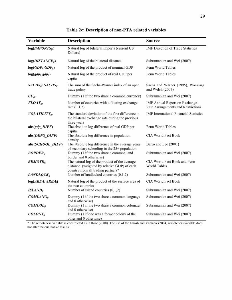
29

Table 2c: Description of non-PTA related variables

Variable Description Source

log(IMPORTSijt) Natural log of bilateral imports (current US Dollars)

IMF Direction of Trade Statistics

log(DISTANCEij) Natural log of the bilateral distance Subramanian and Wei (2007)

log(GDPit GDPjt) Natural log of the product of nominal GDP Penn World Tables

log(gdpit gdpjt) Natural log of the product of real GDP per capita

Penn World Tables

SACHSit+SACHSjt The sum of the Sachs-Warner index of an open trade policy

Sachs and Warner (1995), Wacziarg and Welch (2003)

CUijt Dummy (1 if the two share a common currency) Subramanian and Wei (2007)

FLOATijt Number of countries with a floating exchange rate (0,1,2)

IMF Annual Report on Exchange Rate Arrangements and Restrictions

VOLATILITYijt The standard deviation of the first difference in the bilateral exchange rate during the previous three years

IMF International Financial Statistics

abs(gdp_DIFF) The absolute log difference of real GDP per capita

Penn World Tables

abs(DENS_DIFF) The absolute log difference in population density

CIA World Fact Book

abs(SCHOOL_DIFF) The absolute log difference in the average years of secondary schooling in the 25+ population

Barro and Lee (2001)

BORDERij Dummy (1 if the two share a common land border and 0 otherwise)

Subramanian and Wei (2007)

REMOTEijt The natural log of the product of the average distance (weighted by relative GDP) of each country from all trading partners*

CIA World Fact Book and Penn World Tables

LANDLOCKij Number of landlocked countries (0,1,2) Subramanian and Wei (2007)

log(AREAi AREAj) Natural log of the product of the surface area of the two countries

CIA World Fact Book

ISLANDij Number of island countries (0,1,2) Subramanian and Wei (2007)

COMLANGij Dummy (1 if the two share a common language and 0 otherwise)


COMCOLij Dummy (1 if the two share a common colonizer and 0 otherwise)


COLONYij Dummy (1 if one was a former colony of the other and 0 otherwise)


* The remoteness variable is constructed as in Rose (2000). The use of the Ghosh and Yamarik (2004) remoteness variable does not alter the qualitative results.

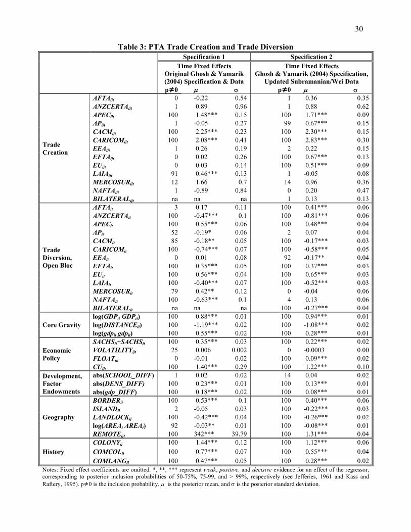
30

Table 3: PTA Trade Creation and Trade Diversion Specification 1 Specification 2

Time Fixed Effects Original Ghosh & Yamarik (2004) Specification & Data

Time Fixed Effects Ghosh & Yamarik (2004) Specification,

Updated Subramanian/Wei Data p≠0 p≠0

Trade Creation

AFTAijt 0 -0.22 0.54 1 0.36 0.35ANZCERTAijt 1 0.89 0.96 1 0.88 0.62APECijt 100 1.48*** 0.15 100 1.71*** 0.09APijt 1 -0.05 0.27 99 0.67*** 0.15CACMijt 100 2.25*** 0.23 100 2.30*** 0.15CARICOMijt 100 2.08*** 0.41 100 2.83*** 0.30EEAijt 1 0.26 0.19 2 0.22 0.15EFTAijt 0 0.02 0.26 100 0.67*** 0.13EUijt 0 0.03 0.14 100 0.51*** 0.09LAIAijt 91 0.46*** 0.13 1 -0.05 0.08MERCOSURijt 12 1.66 0.7 14 0.96 0.36NAFTAijt 1 -0.89 0.84 0 0.20 0.47BILATERALijt na na na 1 0.13 0.13

Trade Diversion, Open Bloc

AFTAit 3 0.17 0.11 100 0.41*** 0.06ANZCERTAit 100 -0.47*** 0.1 100 -0.81*** 0.06APECit 100 0.55*** 0.06 100 0.48*** 0.04APit 52 -0.19* 0.06 2 0.07 0.04CACMit 85 -0.18** 0.05 100 -0.17*** 0.03CARICOMit 100 -0.74*** 0.07 100 -0.58*** 0.05EEAit 0 0.01 0.08 92 -0.17** 0.04EFTAit 100 0.35*** 0.05 100 0.37*** 0.03EUit 100 0.56*** 0.04 100 0.65*** 0.03LAIAit 100 -0.40*** 0.07 100 -0.52*** 0.03MERCOSURit 79 0.42** 0.12 0 -0.04 0.06NAFTAit 100 -0.63*** 0.1 4 0.13 0.06BILATERALit na na na 100 -0.27*** 0.04

Core Gravity log(GDPit GDPjt) 100 0.88*** 0.01 100 0.94*** 0.01log(DISTANCEij) 100 -1.19*** 0.02 100 -1.08*** 0.02log(gdpit gdpjt) 100 0.55*** 0.02 100 0.28*** 0.01

Economic Policy

SACHSit+SACHSjt 100 0.35*** 0.03 100 0.22*** 0.02VOLATILITYijt 25 0.006 0.002 0 -0.0003 0.00FLOATijt 0 -0.01 0.02 100 0.09*** 0.02CUijt 100 1.40*** 0.29 100 1.22*** 0.10

Development, Factor Endowments

abs(SCHOOL_DIFF) 1 0.02 0.02 14 0.04 0.02abs(DENS_DIFF) 100 0.23*** 0.01 100 0.13*** 0.01abs(gdp_DIFF) 100 0.18*** 0.02 100 0.08*** 0.01

Geography

BORDERij 100 0.53*** 0.1 100 0.40*** 0.06ISLANDij 2 -0.05 0.03 100 -0.22*** 0.03LANDLOCKij 100 -0.42*** 0.04 100 -0.26*** 0.02log(AREAi AREAj) 92 -0.03** 0.01 100 -0.08*** 0.01REMOTEijt 100 342*** 39.79 100 1.31*** 0.04

History COLONYij 100 1.44*** 0.12 100 1.12*** 0.06

COMCOLij 100 0.77*** 0.07 100 0.55*** 0.04COMLANGij 100 0.47*** 0.05 100 0.28*** 0.02

Notes: Fixed effect coefficients are omitted. *, **, *** represent weak, positive, and decisive evidence for an effect of the regressor, corresponding to posterior inclusion probabilities of 50-75%, 75-99, and > 99%, respectively (see Jefferies, 1961 and Kass and Raftery, 1995). p≠0 is the inclusion probability, is the posterior mean, and is the posterior standard deviation.

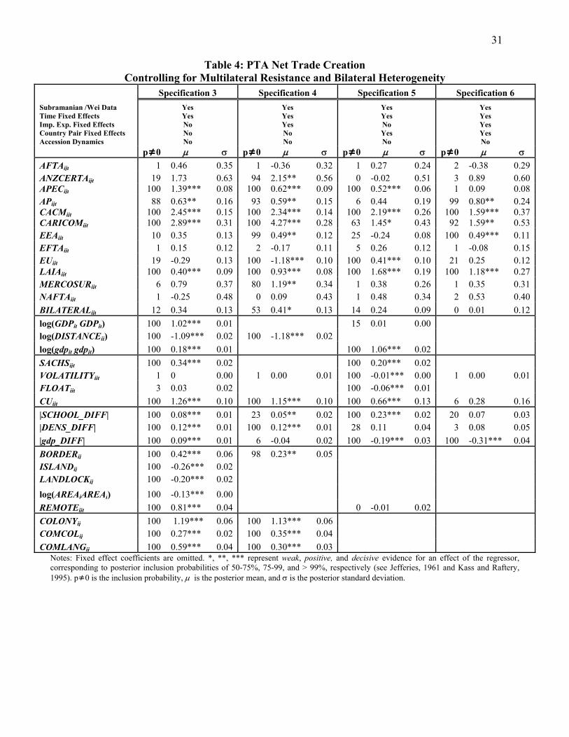
31

Table 4: PTA Net Trade Creation Controlling for Multilateral Resistance and Bilateral Heterogeneity

Specification 3 Specification 4 Specification 5 Specification 6

Subramanian /Wei Data Time Fixed Effects Imp. Exp. Fixed Effects Country Pair Fixed Effects Accession Dynamics

Yes Yes No No No

Yes Yes Yes No No

Yes Yes No Yes No

Yes Yes Yes Yes No

p≠0 p≠0 p≠0 p≠0 AFTAijt 1 0.46 0.35 1 -0.36 0.32 1 0.27 0.24 2 -0.38 0.29ANZCERTAijt 19 1.73 0.63 94 2.15** 0.56 0 -0.02 0.51 3 0.89 0.60APECijt 100 1.39*** 0.08 100 0.62*** 0.09 100 0.52*** 0.06 1 0.09 0.08APijt 88 0.63** 0.16 93 0.59** 0.15 6 0.44 0.19 99 0.80** 0.24CACMijt 100 2.45*** 0.15 100 2.34*** 0.14 100 2.19*** 0.26 100 1.59*** 0.37CARICOMijt 100 2.89*** 0.31 100 4.27*** 0.28 63 1.45* 0.43 92 1.59** 0.53EEAijt 10 0.35 0.13 99 0.49** 0.12 25 -0.24 0.08 100 0.49*** 0.11EFTAijt 1 0.15 0.12 2 -0.17 0.11 5 0.26 0.12 1 -0.08 0.15EUijt 19 -0.29 0.13 100 -1.18*** 0.10 100 0.41*** 0.10 21 0.25 0.12LAIAijt 100 0.40*** 0.09 100 0.93*** 0.08 100 1.68*** 0.19 100 1.18*** 0.27MERCOSURijt 6 0.79 0.37 80 1.19** 0.34 1 0.38 0.26 1 0.35 0.31NAFTAijt 1 -0.25 0.48 0 0.09 0.43 1 0.48 0.34 2 0.53 0.40

BILATERALijt 12 0.34 0.13 53 0.41* 0.13 14 0.24 0.09 0 0.01 0.12

log(GDPit GDPjt) 100 1.02*** 0.01 15 0.01 0.00 log(DISTANCEij) 100 -1.09*** 0.02 100 -1.18*** 0.02

log(gdpit gdpjt) 100 0.18*** 0.01 100 1.06*** 0.02

SACHSijt 100 0.34*** 0.02 100 0.20*** 0.02 VOLATILITYijt 1 0 0.00 1 0.00 0.01 100 -0.01*** 0.00 1 0.00 0.01FLOATijt 3 0.03 0.02 100 -0.06*** 0.01

CUijt 100 1.26*** 0.10 100 1.15*** 0.10 100 0.66*** 0.13 6 0.28 0.16

|SCHOOL_DIFF| 100 0.08*** 0.01 23 0.05** 0.02 100 0.23*** 0.02 20 0.07 0.03|DENS_DIFF| 100 0.12*** 0.01 100 0.12*** 0.01 28 0.11 0.04 3 0.08 0.05

|gdp_DIFF| 100 0.09*** 0.01 6 -0.04 0.02 100 -0.19*** 0.03 100 -0.31*** 0.04

BORDERij 100 0.42*** 0.06 98 0.23** 0.05 ISLANDij 100 -0.26*** 0.02 LANDLOCKij 100 -0.20*** 0.02

log(AREAiAREAj) 100 -0.13*** 0.00

REMOTEijt 100 0.81*** 0.04 0 -0.01 0.02

COLONYij 100 1.19*** 0.06 100 1.13*** 0.06 COMCOLij 100 0.27*** 0.02 100 0.35*** 0.04

COMLANGij 100 0.59*** 0.04 100 0.30*** 0.03 Notes: Fixed effect coefficients are omitted. *, **, *** represent weak, positive, and decisive evidence for an effect of the regressor, corresponding to posterior inclusion probabilities of 50-75%, 75-99, and > 99%, respectively (see Jefferies, 1961 and Kass and Raftery, 1995). p≠0 is the inclusion probability, is the posterior mean, and is the posterior standard deviation.

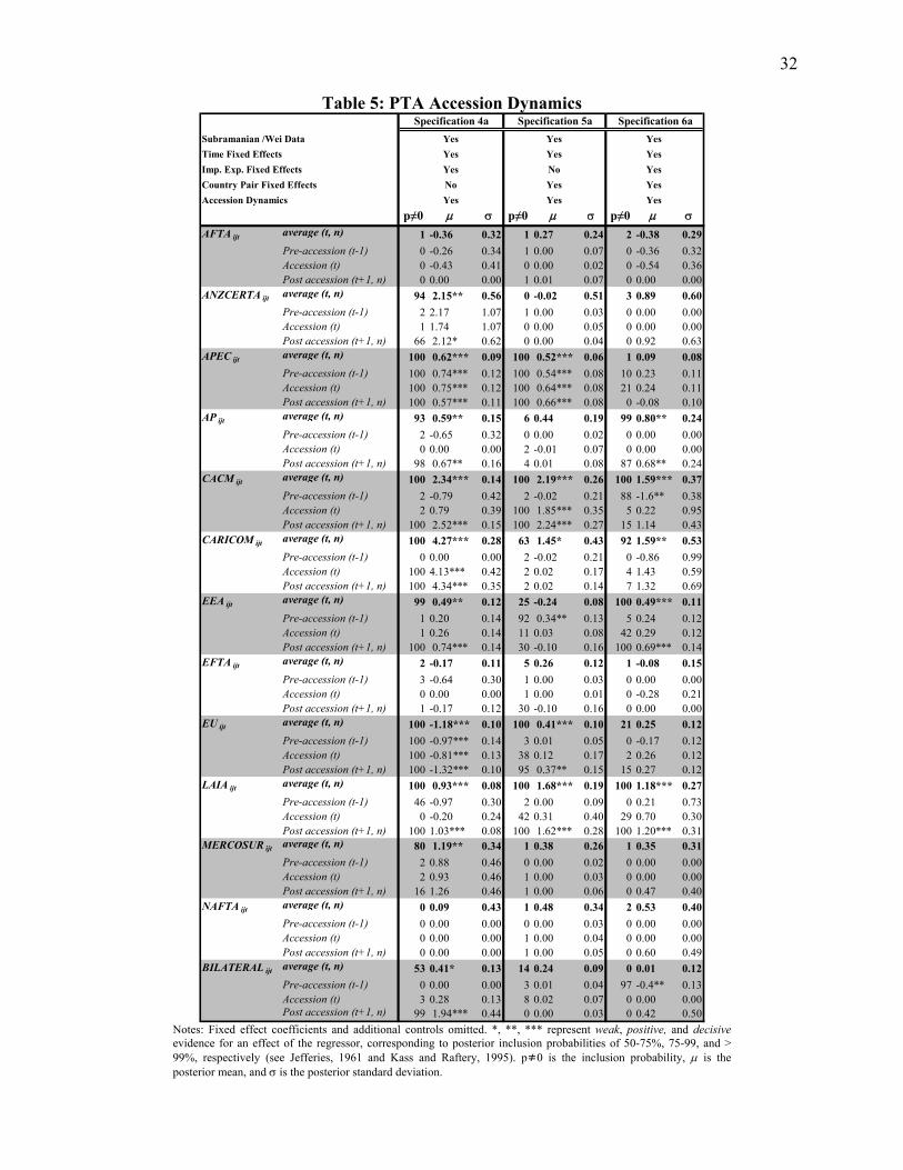
32

Table 5: PTA Accession Dynamics

Subramanian /Wei Data Yes Yes Yes

Time Fixed Effects Yes Yes Yes

Imp. Exp. Fixed Effects Yes No Yes

Country Pair Fixed Effects No Yes Yes

Accession Dynamics Yes Yes Yes

p≠0 p≠0 p≠0 AFTA ijt average (t, n) 1 -0.36 0.32 1 0.27 0.24 2 -0.38 0.29

Pre-accession (t-1) 0 -0.26 0.34 1 0.00 0.07 0 -0.36 0.32Accession (t) 0 -0.43 0.41 0 0.00 0.02 0 -0.54 0.36Post accession (t+1, n) 0 0.00 0.00 1 0.01 0.07 0 0.00 0.00

ANZCERTA ijt average (t, n) 94 2.15** 0.56 0 -0.02 0.51 3 0.89 0.60

Pre-accession (t-1) 2 2.17 1.07 1 0.00 0.03 0 0.00 0.00Accession (t) 1 1.74 1.07 0 0.00 0.05 0 0.00 0.00Post accession (t+1, n) 66 2.12* 0.62 0 0.00 0.04 0 0.92 0.63

APEC ijt average (t, n) 100 0.62*** 0.09 100 0.52*** 0.06 1 0.09 0.08

Pre-accession (t-1) 100 0.74*** 0.12 100 0.54*** 0.08 10 0.23 0.11Accession (t) 100 0.75*** 0.12 100 0.64*** 0.08 21 0.24 0.11Post accession (t+1, n) 100 0.57*** 0.11 100 0.66*** 0.08 0 -0.08 0.10

AP ijt average (t, n) 93 0.59** 0.15 6 0.44 0.19 99 0.80** 0.24

Pre-accession (t-1) 2 -0.65 0.32 0 0.00 0.02 0 0.00 0.00Accession (t) 0 0.00 0.00 2 -0.01 0.07 0 0.00 0.00Post accession (t+1, n) 98 0.67** 0.16 4 0.01 0.08 87 0.68** 0.24

CACM ijt average (t, n) 100 2.34*** 0.14 100 2.19*** 0.26 100 1.59*** 0.37

Pre-accession (t-1) 2 -0.79 0.42 2 -0.02 0.21 88 -1.6** 0.38Accession (t) 2 0.79 0.39 100 1.85*** 0.35 5 0.22 0.95Post accession (t+1, n) 100 2.52*** 0.15 100 2.24*** 0.27 15 1.14 0.43

CARICOM ijt average (t, n) 100 4.27*** 0.28 63 1.45* 0.43 92 1.59** 0.53

Pre-accession (t-1) 0 0.00 0.00 2 -0.02 0.21 0 -0.86 0.99Accession (t) 100 4.13*** 0.42 2 0.02 0.17 4 1.43 0.59Post accession (t+1, n) 100 4.34*** 0.35 2 0.02 0.14 7 1.32 0.69

EEA ijt average (t, n) 99 0.49** 0.12 25 -0.24 0.08 100 0.49*** 0.11

Pre-accession (t-1) 1 0.20 0.14 92 0.34** 0.13 5 0.24 0.12Accession (t) 1 0.26 0.14 11 0.03 0.08 42 0.29 0.12Post accession (t+1, n) 100 0.74*** 0.14 30 -0.10 0.16 100 0.69*** 0.14

EFTA ijt average (t, n) 2 -0.17 0.11 5 0.26 0.12 1 -0.08 0.15

Pre-accession (t-1) 3 -0.64 0.30 1 0.00 0.03 0 0.00 0.00Accession (t) 0 0.00 0.00 1 0.00 0.01 0 -0.28 0.21Post accession (t+1, n) 1 -0.17 0.12 30 -0.10 0.16 0 0.00 0.00

EU ijt average (t, n) 100 -1.18*** 0.10 100 0.41*** 0.10 21 0.25 0.12

Pre-accession (t-1) 100 -0.97*** 0.14 3 0.01 0.05 0 -0.17 0.12Accession (t) 100 -0.81*** 0.13 38 0.12 0.17 2 0.26 0.12Post accession (t+1, n) 100 -1.32*** 0.10 95 0.37** 0.15 15 0.27 0.12

LAIA ijt average (t, n) 100 0.93*** 0.08 100 1.68*** 0.19 100 1.18*** 0.27

Pre-accession (t-1) 46 -0.97 0.30 2 0.00 0.09 0 0.21 0.73Accession (t) 0 -0.20 0.24 42 0.31 0.40 29 0.70 0.30Post accession (t+1, n) 100 1.03*** 0.08 100 1.62*** 0.28 100 1.20*** 0.31

MERCOSUR ijt average (t, n) 80 1.19** 0.34 1 0.38 0.26 1 0.35 0.31

Pre-accession (t-1) 2 0.88 0.46 0 0.00 0.02 0 0.00 0.00Accession (t) 2 0.93 0.46 1 0.00 0.03 0 0.00 0.00Post accession (t+1, n) 16 1.26 0.46 1 0.00 0.06 0 0.47 0.40

NAFTA ijt average (t, n) 0 0.09 0.43 1 0.48 0.34 2 0.53 0.40

Pre-accession (t-1) 0 0.00 0.00 0 0.00 0.03 0 0.00 0.00Accession (t) 0 0.00 0.00 1 0.00 0.04 0 0.00 0.00Post accession (t+1, n) 0 0.00 0.00 1 0.00 0.05 0 0.60 0.49

BILATERAL ijt average (t, n) 53 0.41* 0.13 14 0.24 0.09 0 0.01 0.12

Pre-accession (t-1) 0 0.00 0.00 3 0.01 0.04 97 -0.4** 0.13Accession (t) 3 0.28 0.13 8 0.02 0.07 0 0.00 0.00

Post accession (t+1, n) 99 1.94*** 0.44 0 0.00 0.03 0 0.42 0.50

Specification 5a Specification 6aSpecification 4a

Notes: Fixed effect coefficients and additional controls omitted. *, **, *** represent weak, positive, and decisive evidence for an effect of the regressor, corresponding to posterior inclusion probabilities of 50-75%, 75-99, and > 99%, respectively (see Jefferies, 1961 and Kass and Raftery, 1995). p≠0 is the inclusion probability, is the posterior mean, and is the posterior standard deviation.

trade creation and diversion revisited: accounting for model

Documents