tragedy of the commons - economics research unit at tu wien
TRANSCRIPT
Agent-Based Modelling in Economics, First Edition. Lynne Hamill and Nigel Gilbert. © 2016 John Wiley & Sons, Ltd. Published 2016 by John Wiley & Sons, Ltd.
Tragedy of the commons
10
10.1 Introduction
The term ‘tragedy of the commons’ was coined in 1968 by Garrett Hardin, a professor of biology at the University of California, Santa Barbara. His famous paper (Hardin, 1968) primarily addressed the problem of human overpopulation and argued that technology could not be relied on to accommodate ever‐increasing numbers: social changes were required to limit the population. As one example among several, he described a pasture open to all and argued that, eventually, if each herdsman behaved rationally and pursued his own interest by adding animals to the pasture, the ‘tragedy of the commons’ would ensue because the pasture could not support an ever‐increasing number of animals. Thus, the herdsman pursuing his own private interest did not pro-mote the interest of the community as a whole: Adam Smith’s invisible hand (see Box 5.4) was not at work. But this analysis fails to acknowledge that people have found ways of avoiding the ‘tragedy of the commons’ by cooperating. For instance, Nobel laureate Elinor Ostrom (1990, pp.58–88) described systems that have persisted for hundreds of years for managing alpine pas-tures in Switzerland, forests in Japan and water for irrigation in Spain, while Straughton (2008) described the management of moorlands in northern England.
Before discussing the issues, we first define exactly what we mean by ‘commons’. Formally, a ‘common pool resource’ (CPR) is ‘a natural or man‐made resource system that is sufficiently large as to make it costly (but not impossible) to exclude potential beneficiaries from obtaining benefits from its use’ (Ostrom, 1990, p.30). In economic terms, a CPR is not a public good because it is a limited resource and use by one person means that it cannot be used by another. Indeed, it is because the CPR is a limited resource that the problem of management arises. In con-trast, the use of a public good by one person does not reduce its availability for another, for example, a weather forecast (Ostrom, 1990, pp.31–32).
There are many different types of CPRs, and each has its own distinct characteristics requiring different management arrangements to make best use of it. For example, compared to managing grazing, forestry involves very long time horizons, while the management of fisheries has to
TRAGEdy OF THE COmmONS 215
accommodate the movement of fish. Both forestry and fishery are covered in detail in Perman et al. (2003: Chapters 17 & 18), which is also a useful introduction to this area of economics.
This chapter focuses on grazing because it is simpler and it is the typical CPR found in England. (See Box 10.1 for background on English common land.) Following Natural England (2014), we call those with the right to use the common ‘commoners’.
Economic analysis
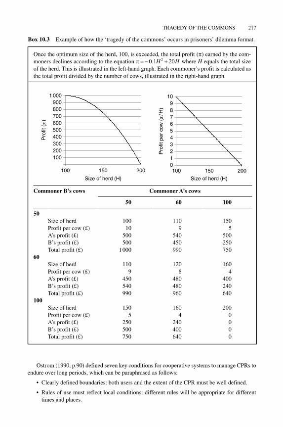
Game theory is sometimes applied to the CPR problem, representing it as a prisoner’s dilemma game (see Box 10.2). To model the ‘tragedy of the commons’ in this way, two commoners share a pasture, and instead of jail sentences, the reward matrix shows how benefits vary with the number of animals grazed. In our example, the optimum herd size is 100, and this produces a total profit of £1000. If the optimum size of the herd is exceeded, the total profit declines. In the real world, this would perhaps happen because the cows are in poorer condition. In this example, profit ( ) earned by the commoners declines according to the equation
0 1 202. H H
where H equals the number of cows, the total size of the herd: thus, if there are 200 cows, the total profit is zero. This is illustrated in the top part of Box 10.3. If the two commoners share equally and both put half the optimum number of cows on the pasture, they both earn the same income of £500 and the total profit is maximised. However, if one commoner ‘defects’ by putting 60 cows on the pasture while the other puts only 50, then the herd size rises to 110. Given the profit function above, the total profit falls to £990 or £9 per cow. Nevertheless, the ‘defector’ gains at the expense of the other, with a total gain of 60 × £9 = £540 instead of £500 under the optimum scenario. However, the other commoner receives less than the optimum, only 50 × £9 = £450 instead of £500. If both commoners think the other will put 60 cows on the common, both have an incentive to graze 60 cows. The total herd size then rises to 120 and the total gain falls to £960 or £8 per cow. Both commoners therefore receive £480, and both are worse off than in the optimum scenario. If this continues to the extreme and each commoner puts 100 cows on the pasture, the tragedy occurs and both commoners get no income. The reward matrix is shown in the lower part of Box 10.3. The precise figures are not important, but simply illustrate the principle, namely, that the incentives for individuals are such that they bring about an outcome that is undesirable for all.
But setting out the tragedy in this way demonstrates why the prisoner’s dilemma is not applicable to this situation. The simple, single prisoner’s dilemma game assumes that there is no
In England, Parliament has made laws on common land since the thirteenth century (Natural England, 2014; Straughton, 2008, p.10). The Commons Act 2006 brought together in one Act of Parliament all the common land legislation passed in the previous 700 years (Natural England, 2014). The 2006 Act aims to protect common land ‘in a sustainable manner delivering benefits for farming, public access and biodiversity’ (dEFRA, 2014).
There is a popular misconception that common land belongs to everyone, but that is not the case (Natural England, 2014). In England, common land is privately owned land over which third parties have certain rights (Straughton, 2008, p.9).
There are currently just over 7000 commons in England, together accounting for 3% of the land area; much is poor‐quality grazing (Natural England, 2014).
Box 10.1 Common land in England.
216 AGENT-BASEd mOdEllING IN ECONOmICS
communication and no cooperation and the commoners have no regard for the future. People do not always act in their short‐term interest: they care about the long‐term future, be it their own or that of their children. In a stable society in which people expect that they and their families will continue to live and work alongside one another for years or even generations, the kind of behav-iour implied by the prisoner’s dilemmas is unlikely. The key characteristic of the prisoners’ dilemma is that cooperation is forbidden. (For further discussion, see Ostrom, 1990, pp.2–20.) Similarly, in the Cournot–Nash equilibrium problem discussed in Chapter 6, there was no coop-eration allowed. Indeed, the Cournot–Nash model presented in Chapter 6 can be adapted to model uncooperative behaviour in this context. However, in this chapter, we focus on cooperation.
However, it is not clear how cooperation emerges. Ostrom (1990) suggests that it is a slow, protracted process. Game theory based on an unlimited number of repeated games may provide a clue. If a prisoner’s dilemma game is repeated indefinitely, a ‘tit‐for‐tat’ strategy – in which each player copies what the other player did in the previous round – cooperation can emerge. (See, for instance, Varian, 2010, pp.529–530.) Here, we extend the prisoner’s dilemma example by increasing the number of commoners to 10. Now, on the basis of the example used earlier, and assuming that the size of the herd is 150, compared to the optimum of 100, then it is clearly beneficial overall if the herd size were to be reduced. But if one of the commoners reduces the number of their cows, the group as a whole will gain but the reducer will lose out. At the other extreme, if all reduce the number of their cows, all benefit too. In this example, it is possible for both the group and all individuals to benefit if just four commoners reduce the number of their cows. This is illustrated in Table 10.1. It demonstrates how cooperation might start. Again, the precise numbers are not important.
The scenario is as follows. Two friends are suspected of committing a crime and are taken into police custody. They are put in separate cells, so that they cannot communicate with each other. They are both told:
• If you do not confess, but your friend does, you will get a sentence of 10 years.
• If you confess, you will only get a sentence of 5 years.
• If neither of you confess, we will charge you with a lesser crime, and you will still get a sentence, but only a year.
The reward matrix looks like this with the sentences shown as, for example, (10, 5), meaning that A gets 10 years and B gets 5 years.
Suspect B Suspect A
Confesses does not confess
Confesses (5, 5) (10, 5)does not confess (5, 10) (1, 1)
It is in the interests of both not to confess, and then each would receive a sentence of one year. But if A does not confess and B does, then A will receive the maximum sentence. And the same holds for B. Neither knows what the other will do. Consequently, both will probably confess in order to avoid the maximum sentence, and each will get 5 years.
For more information on game theory and the prisoner’s dilemma, see, for example, Varian (2010: Chapters 28 & 29) or Begg et al. (2011, pp. 206–212).
Box 10.2 Prisoner’s dilemma and the ‘tragedy of the commons’.
TRAGEdy OF THE COmmONS 217
Ostrom (1990, p.90) defined seven key conditions for cooperative systems to manage CPRs to endure over long periods, which can be paraphrased as follows:
• Clearly defined boundaries: both users and the extent of the CPR must be well defined.
• Rules of use must reflect local conditions: different rules will be appropriate for different times and places.
Once the optimum size of the herd, 100, is exceeded, the total profit ( ) earned by the com-moners declines according to the equation 0 1 202. H H where H equals the total size of the herd. This is illustrated in the left‐hand graph. Each commoner’s profit is calculated as the total profit divided by the number of cows, illustrated in the right‐hand graph.
100 200 300 400 500 600 700 800 900
1 000
100 150 200
Pro
fit (
π)
Size of herd (H)
0123456789
10
100 150 200
Pro
fit p
er c
ow (
π/H
)
Size of herd (H)
Commoner B’s cows Commoner A’s cows
50 60 100
50Size of herd 100 110 150Profit per cow (£) 10 9 5A’s profit (£) 500 540 500B’s profit (£) 500 450 250Total profit (£) 1 000 990 750
60Size of herd 110 120 160Profit per cow (£) 9 8 4A’s profit (£) 450 480 400B’s profit (£) 540 480 240Total profit (£) 990 960 640
100Size of herd 150 160 200Profit per cow (£) 5 4 0A’s profit (£) 250 240 0B’s profit (£) 500 400 0Total profit (£) 750 640 0
Box 10.3 Example of how the ‘tragedy of the commons’ occurs in prisoners’ dilemma format.
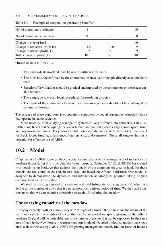
218 AGENT-BASEd mOdEllING IN ECONOmICS
• most individuals involved must be able to influence the rules.
• The rules must be enforced by the commoners themselves or people directly accountable to them.
• Sanctions for violations should be gradual and imposed by the commoners or those account-able to them.
• There must be low‐cost, local procedures for resolving disputes.
• The rights of the commoners to make their own arrangements should not be challenged by external authorities.
The essence of these conditions is cooperation, supported by social constraints, especially those that operate in stable societies.
more recently, after studying a range of systems in very different environments, liu et al. (2007) concluded that ‘couplings between human and natural systems vary across space, time, and organizational units. They also exhibit nonlinear dynamics with thresholds, reciprocal feedback loops, time lags, resilience, heterogeneity, and surprises’. These all suggest there is a potential for effective use of ABm.
10.2 Model
Chapman et al. (2009) have produced a detailed simulation of the management of moorlands in northern England, but this is too detailed for our purpose. Schindler (2012a & 2012b) has created two models using Netlogo that address the tragedy of the commons on grazing land, but these models are too complicated and, in one case, are based on African herdsmen. Our model is designed to demonstrate the dynamics and interaction as simply as possible taking English common land as its inspiration.
We start by creating a model of a meadow and establishing its ‘carrying capacity’, which we define as the number of cows that it can support over a given period of time. We then add com-moners so that we can examine alternative strategies for sharing the meadow.
The carrying capacity of the meadow
‘Carrying capacity’ will, of course, vary with the type of animals, the climate and the nature of the soil. For example, the number of sheep that can be supported on sparse grazing on the hills in northern England will be quite different to the number of ponies that can be supported by the same area of land in the New Forest in warmer southern England. detailed biological models have been built such as Armstrong et al.’s (1997) hill grazing management model. But our focus of interest
Table 10.1 Example of cooperation generating benefitsa.
No. of commoners reducing 1 4 10
No. of commoners unchanged 9 6 0
Change in size of herd −1 −4 −10Change in reducers’ profit (£) −3.6 0.6 9Change in other’s profit (£) 1.5 6 9Total change in profit (£) 10 38 90
a Based on data in Box 10.3.

TRAGEdy OF THE COmmONS 219
is not on the detailed biological processes but the strategies adopted by commoners; so at this stage, we keep our modelling of biological processes as simple as possible, although we draw very broadly on data for the United Kingdom such as EBlEX (2013).
The rate at which grass grows depends on all sorts of factors and varies during the year. In England, it is faster in the spring and early autumn and less in the summer and barely grows at all in winter. Here, we focus on summer grazing and for simplicity assume that grass grows at the same rate throughout the period. The growth of grass is modelled using a logistic function fol-lowing Perman et al. (2003, p.562). logistic functions are explained in Box 10.4. For example, if a cow grazes a patch of grass down to 0.25 of its maximum, the grass growth rate is set at 0.2 per week, and a grazed patch is not grazed again until it reaches 0.9 of its maximum, it will take 16 weeks for a grazed patch to recover sufficiently to be grazed again. This is illustrated at the
The logistic equation, devised by Verhulst in 1838 to describe the growth of populations, can be used to produce a simple non‐linear model in which the change depends on the level in the previous period and the growth rate (Strogatz, 1994, pp. 9–10 & 22–23).
If Gt is the amount of grass at time t and g the rate at which grass grows each week, then the amount of grass in the next week is given by
G G G G gt t t t1 1
where 0 1Gt and 1g .For example, if Gt equals 0.25 and g is set at 0.2, then after 1 week, Gt 1 will be 0.2875:
Gt 1 0 25 0 25 0 75 0 2 0 2875. . . . .
If, however, the grass has nearly reached its maximum, the absolute level of growth will be much lower. For example, if Gt equals 0.95 and g is set at 0.2, then after 1 week, Gt 1 will be 0.9595:
Gt 1 0 95 0 95 0 05 0 2 0 9595. . . . .
Example of grass growing at rate of 0.2 per week. If it is grazed down to 0.25, it will recover to 0.9 after 16 weeks.
Box 10.4 Grass growth using a logistic function.
0.0
0.1
0.2
0.3
0.4
0.5
0.6
0.7
0.8
0.9
1.0
0 2 4 6 8 10 12 14 16 18 20 22 24
Am
ount
of g
rass
Weeks

220 AGENT-BASEd mOdEllING IN ECONOmICS
bottom of Box 10.4. These parameter values have been chosen to ensure that the carrying capacity is a reasonably small number of cows in order to reduce the time taken by each run.
The model meadow comprises 9999 patches. Initially, each patch has 1 unit of grass. The modeller sets the initial number of cows, and these cows are distributed randomly. Each cow then eats 0.75 units of grass and the next week moves on to the nearest unoccupied patch with sufficient grass, defined at 0.9 units. (Cows are not allowed to eat all the grass on a patch as it will not then regrow!) If a cow cannot find a suitable patch, it dies.
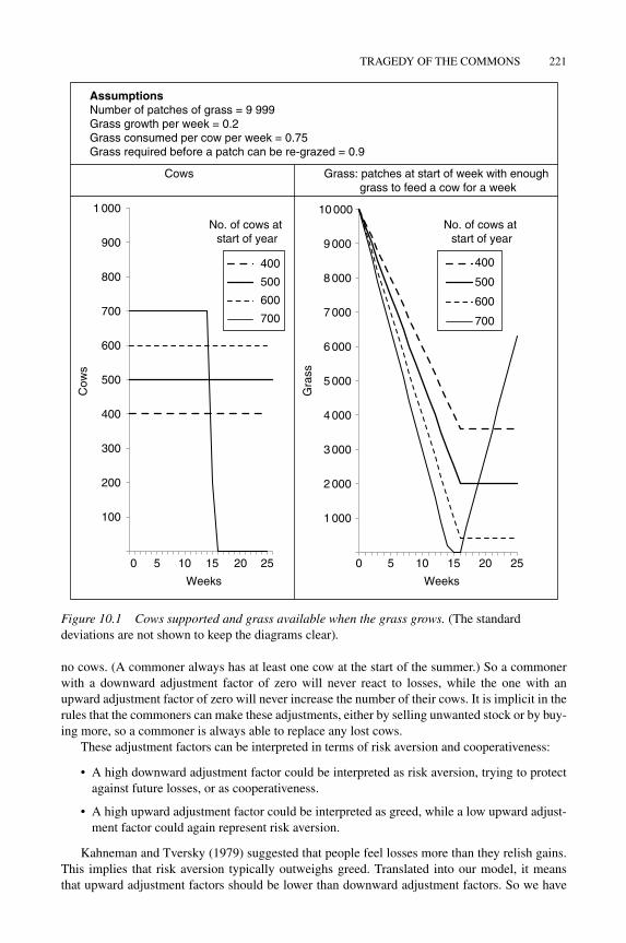
If the cows eat the grass faster than it grows, the pasture available will decline. As the rate at which grass grows is fixed, if there are too many cows, the pasture will be overgrazed and the cattle will starve. The model runs for 25 weeks to represent a summer of grazing. To establish the basic characteristics of the model, we start by assuming that the grass does not grow. With 400 cows, each consuming 1 patch of grass a week, then the meadow will support all the cows for 25 weeks. The model produces this result.
Allowing the grass to grow a little each week transforms this scenario. Using a growth rate of 0.2 (as illustrated in Box 10.4), as many as 600 cows will survive the summer season although very little grass is then left by the end, suggesting that this level of use will not be sustainable in the long run. However, if there are more than 700 cows, they cannot survive the summer: the grass runs out after 16 weeks. This is shown in Figure 10.1.
more information on this model – the Carrying capacity model – is in Appendix 10.A.
Managing the meadow
Having established the characteristics of the model meadow, in particular its carrying capacity, we now introduce commoners to manage the cattle.
Instead of modelling just one summer’s grazing, the meadow management model covers many years. Of course, in reality, the rate of growth of the grass and thus the carrying capacity would vary from year to year. But in order to be able to draw out the key dynamics, it is assumed that the grass grows at the same rate in all years. As before, the cows graze for 25 weeks. They are then removed and the grass has the opportunity to recover a little: it is assumed that there are only 5 weeks of growth, reflecting the fact that grass in England grows only a little over winter. (See, e.g. EBlEX, 2013.)
There are 10 commoners and at the start of the run the number of cows – set at 300 in our examples – is divided equally between them. At the beginning of each year, the commoners decide whether to increase or reduce the number the cows they will graze that summer. In the examples used in the introduction, the commoners made their decisions on the basis of a loss function. In the model, the grazing of the meadow in effect replaces this loss function in that it determines how many cows survive and thus how much money the commoners make. We also saw in the introduction how, if a few commoners responded to a loss by cutting back, the situation could be improved for everyone. Based on this, a pair of simple heuristic decision rules is used:
• If all the commoner’s cows survive the summer, the commoner increases their herd by an upward factor, to reflect an incentive to take more.
• If all the cows do not survive, the commoner reduces the size of their herd by a downward factor, to reflect a dislike of losses.
Each commoner is randomly allocated a downward and an upward factor based on a normal distribution with a mean set by the modeller and the standard deviation set equal to the mean. The upward and downward factors cannot be negative but can be zero and are arbitrarily constrained to be less than one in order to avoid any commoner making very large increases or being left with
TRAGEdy OF THE COmmONS 221
no cows. (A commoner always has at least one cow at the start of the summer.) So a commoner with a downward adjustment factor of zero will never react to losses, while the one with an upward adjustment factor of zero will never increase the number of their cows. It is implicit in the rules that the commoners can make these adjustments, either by selling unwanted stock or by buy-ing more, so a commoner is always able to replace any lost cows.
These adjustment factors can be interpreted in terms of risk aversion and cooperativeness:
• A high downward adjustment factor could be interpreted as risk aversion, trying to protect against future losses, or as cooperativeness.
• A high upward adjustment factor could be interpreted as greed, while a low upward adjust-ment factor could again represent risk aversion.
Kahneman and Tversky (1979) suggested that people feel losses more than they relish gains. This implies that risk aversion typically outweighs greed. Translated into our model, it means that upward adjustment factors should be lower than downward adjustment factors. So we have
AssumptionsNumber of patches of grass = 9 999Grass growth per week = 0.2Grass consumed per cow per week = 0.75Grass required before a patch can be re-grazed = 0.9
Cows Grass: patches at start of week with enough grass to feed a cow for a week
100
200
300
400
500
600
700
800
900
1 000
0 5 10 15 20 25
Cow
s
Weeks
400
500
600
700
No. of cows at start of year
1 000
2 000
3 000
4 000
5 000
6 000
7 000
8 000
9 000
10 000
0 5 10 15 20 25
Gra
ss
Weeks
400
500
600
700
No. of cows at start of year
Figure 10.1 Cows supported and grass available when the grass grows. (The standard deviations are not shown to keep the diagrams clear).

222 AGENT-BASEd mOdEllING IN ECONOmICS
arbitrarily combined a downward adjustment factor based on a distribution with a mean of 0.5 with an upward adjustment with a mean of 0.1.
Putting aside the factors determining the rates of grass growth and consumption – which are set as in the carrying capacity model – the modeller can set just these factors:
• The initial number of cows
• The means (and standard deviations) of the downward and upward adjustment factors
• Whether there is a limit on the number of cows any commoner can graze on the meadow and, if so, what that number is (but more will be said about this later)
• The number of years that the model will run.
The model records the number of cows at the start of each summer grazing season and the number at the end, both in total and for each commoner.
AssumptionsMeadow assumptions as in Figure 10.1300 cows initially evenly distrubuted across 10 commonersMean (and standard deviation) of distribution of downward adjustment factor = 0.5Mean (and standard deviation) of distribution of upward adjustment factor = 0.1Limit = 1000 per commoner
Each line represents a run, but not all 15 are visible due to overlap
100
200
300
400
500
600
1 2 3 4 5 6 7 8 9 10 1112 13 14 15 16 17 18 19 20 21 22 23 24 25
Tot
al c
ows
at e
nd o
f yea
r
Years
0
100
200
300
400
500
600
700
1 2 3 4 5 6 7 8 9 10 11 12 13 14 15 16 17 18 19 20 21 22 23 24 25
Tot
al c
ows
at e
nd o
f yea
r
Years
Mean(solid line) and plus and minus one standard deviation (dotted lines) in number of cows at the end of year
Figure 10.2 Meadow management model results: limit of 1000 cows per commoner. 15 runs over 25 years.

TRAGEdy OF THE COmmONS 223
The aim is to establish how best to create sustainable stability. Four indicators are used:
• The average number of cows at the end of each year: the more the better.
• The survival rate: the percentage of cows that survive the summer. The higher this number, the better and ideally the survival rate should be 100%.
• The proportion of years in which some cows die, that is, the survival rate is less than 100%. The lower this number, the better: ideally, it should be zero.
• Whether there is any variation in the number of cows at the end of year during the last 10 years: the less variation, the better and ideally there should be none, indicating that the system is stable.
Furthermore, comparing the first three indicators calculated over all 25 years with the same indicators calculated over just the last 10 years shows whether the system is becoming more sus-tainable and stable over time. It is important to consider these four indicators together. For example, it would not be an efficient use of the resources provided by the meadow if there were on average only 100 cows grazing even if the survival rate was then always 100% and the number of cows on the common was constant as we know that the meadow can support significantly more.
To explore the dynamics of this simple model, we start by setting the limit for each commoner at 1000, which in effect means there is no limit as this level is way above the total carrying capacity of the meadow. Each commoner starts with 30 cows. The model is run 15 times for 25 years. Figure 10.2 shows the number of cows at the end of each year: it is highly volatile. For example, after 5 years, the number of cows at the end of any given year often ranges from zero to over 500 from one run to another. Furthermore, although the commoners all start with the same number of cows, by the end of the 25th year, most of the cows being grazed tend to belong to just one or two com-moners. When there are any cows left at all, on average, one commoner owns 58% (sd 18). How this concentration arises is shown in Box 10.5 which uses actual examples from one of these runs.
What then might bring more stability to this system? A rule found in both England (Straughton, 2008, p.119) and Switzerland (Ostrom, 1990, pp.61–65) is that commoners are allowed to put on the common land pasture the same number of animals that they can support over winter. In prac-tice, this means those with larger farms will be able to put more animals on the common because they have more land with which to produce forage (such as hay) to feed to the animals during the winter months when there is no grass available. This prevents commoners buying in animals to graze on the commons over the summer to sell on before winter. For simplicity, we have assumed that the limit for each commoner is set at the same level and leave it as an exercise for readers with programming skills to explore the impact of an unequal distribution. This limit could be enforced by some well‐informed public official, or it could evolve over time as Ostrom’s work suggests.
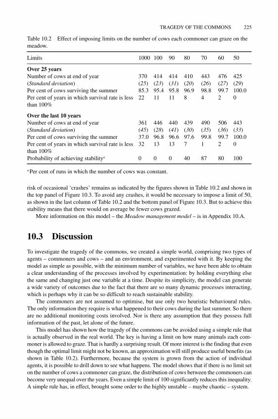
We know that the carrying capacity of the meadow is less than 700 cows. However, even if the limit were set at 100 per commoner, thus potentially allowing up to 1000 cows in total, there is still a significant improvement in all four indicators compared to when there is in effect no limit. The first two columns of Table 10.2 show that with a limit of 100 per commoner, the meadow supports more cows than when there is no limit: on average, 414 with a survival rate of 95% instead of 370 with a survival rate of 85%. Also, with this limit, the indicators over the last 10 years are better than for the period as a whole, while this is not the case for when there is no limit. Furthermore, the extreme inequality in the distribution of cows across the commoners is reduced. With a limit of 100 cows per commoner, after 25 years on average, the commoner with the most cows on the meadow has 22% (sd 3) of the total.
Reducing the limits increases the benefits. Arguably, a limit of 60 cows per commoner pro-duces the best results, with an average of 476 cows being grazed with a survival rate of 99.7%. With a limit of 60 cows per commoner, there is only a slight increase in inequality over 25 years, and on average, 7 of the 10 commoners have the maximum number of cows permitted. But the

A’s downward adjustment factor = 0.5 and upward adjustment factor = 0.1B’s downward adjustment factor = 0.5 and upward adjustment factor = 0.2Both commoners start with 30 cows, as do all the other commoners.
In year 1, all A’s cows survive, and so in year 2, A grazes 30 × 1.1 = 33 cows. All B’s sur-vive too, but B increases the number of cows in year 2 to 30 × 1.2 = 36.
This continues until year 11, by which time at the start of the year A puts 72 cows on the common and B 177. In total, the 10 commoners put 573 cows on the common. This overloads the common, and only 330 survive, including 42 belonging to A and 98 belonging to B. Following the adjustment rule, the next year, both graze only half as many as at the start of the previous year: A grazes 36 (72 × 0.5) and B 89 (177 × 0.5).
All is well until year 19. At the start of that year, A puts 66 cows on the meadow and B 313. In total, the 10 commoners put 598 cows on the common. The meadow cannot support this number and all but are 86 lost. Just 11 of A’s cows and 50 of B’s survive. The next year, year 20, A puts out 33 and B 157, being half of the number with which they started the previous year.
Each year, all the other commoners put more cows on the common until in year 25 there is another crash. By the end of year 25, there are just 182 cows on the common, of which A has 17 and B has 118.
Short bars mean that the number of cows at the end of the year was the same as at the start. long bars mean that the number of cows dropped during the year, that is, less than 100% survived.
Commoner A’s cows Commoner B’s cows
All 10 commoners
0100200300400500600700
1 2 3 4 5 6 7 8 9 10 11 12 13 14 15 16 17 18 19 20 21 22 23 24 25Tot
al c
ows
at e
nd o
f yea
r
Years
0
50
100
150
200
250
300
350
400
1 3 5 7 9 1113151719212325
Cow
s at
end
of y
ear
Years
0
50
100
150
200
250
300
350
400
1 3 5 7 9 11 13 151719 21 23 25
Cow
s at
end
of y
ear
Years
Box 10.5 Examples of commoners’ experiences.
TRAGEdy OF THE COmmONS 225
risk of occasional ‘crashes’ remains as indicated by the figures shown in Table 10.2 and shown in the top panel of Figure 10.3. To avoid any crashes, it would be necessary to impose a limit of 50, as shown in the last column of Table 10.2 and the bottom panel of Figure 10.3. But to achieve this stability means that there would on average be fewer cows grazed.
more information on this model – the Meadow management model – is in Appendix 10.A.
10.3 Discussion
To investigate the tragedy of the commons, we created a simple world, comprising two types of agents – commoners and cows – and an environment, and experimented with it. By keeping the model as simple as possible, with the minimum number of variables, we have been able to obtain a clear understanding of the processes involved by experimentation: by holding everything else the same and changing just one variable at a time. despite its simplicity, the model can generate a wide variety of outcomes due to the fact that there are so many dynamic processes interacting, which is perhaps why it can be so difficult to reach sustainable stability.
The commoners are not assumed to optimise, but use only two heuristic behavioural rules. The only information they require is what happened to their cows during the last summer. So there are no additional monitoring costs involved. Nor is there any assumption that they possess full information of the past, let alone of the future.
This model has shown how the tragedy of the commons can be avoided using a simple rule that is actually observed in the real world. The key is having a limit on how many animals each com-moner is allowed to graze. That is hardly a surprising result. Of more interest is the finding that even though the optimal limit might not be known, an approximation will still produce useful benefits (as shown in Table 10.2). Furthermore, because the system is grown from the action of individual agents, it is possible to drill down to see what happens. The model shows that if there is no limit set on the number of cows a commoner can graze, the distribution of cows between the commoners can become very unequal over the years. Even a simple limit of 100 significantly reduces this inequality. A simple rule has, in effect, brought some order to the highly unstable – maybe chaotic – system.
Table 10.2 Effect of imposing limits on the number of cows each commoner can graze on the meadow.
limits 1000 100 90 80 70 60 50
Over 25 yearsNumber of cows at end of year 370 414 414 410 443 476 425(Standard deviation) (25) (23) (31) (20) (26) (27) (29)Per cent of cows surviving the summer 85.3 95.4 95.8 96.9 98.8 99.7 100.0Per cent of years in which survival rate is less than 100%
22 11 11 8 4 2 0
Over the last 10 yearsNumber of cows at end of year 361 446 440 439 490 506 443(Standard deviation) (45) (28) (41) (30) (35) (36) (33)Per cent of cows surviving the summer 37.0 96.8 96.6 97.6 99.8 99.7 100.0Per cent of years in which survival rate is less than 100%
32 13 13 7 1 2 0
Probability of achieving stabilitya 0 0 0 40 87 80 100
a Per cent of runs in which the number of cows was constant.
226 AGENT-BASEd mOdEllING IN ECONOmICS
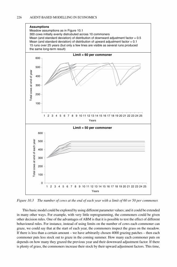
This basic model could be explored by using different parameter values; and it could be extended in many other ways. For example, with very little reprogramming, the commoners could be given other decision rules. One of the advantages of ABm is that it is possible to test the effect of different behavioural rules. For instance, instead of using limits on the number of cows each commoner can graze, we could say that at the start of each year, the commoners inspect the grass on the meadow. If there is less than a certain amount – we have arbitrarily chosen 4000 grazing patches – then each commoner puts less stock out to graze in the coming summer. How many each commoner puts on depends on how many they grazed the previous year and their downward adjustment factor. If there is plenty of grass, the commoners increase their stock by their upward adjustment factors. This time,
AssumptionsMeadow assumptions as in Figure 10.1300 cows initially evenly distrubuted across 10 commonersMean (and standard deviation) of distribution of downward adjustment factor = 0.5Mean (and standard deviation) of distribution of upward adjustment factor = 0.115 runs over 25 years (but only a few lines are visible as several runs produced the same long-term result)
100
200
300
400
500
600
1 2 3 4 5 6 7 8 9 10 11 12 13 14 15 16 17 18 19 20 21 22 23 24 25
Tot
al c
ows
at e
nd o
f yea
r
Years
0
100
200
300
400
500
600
1 2 3 4 5 6 7 8 9 10 11 12 13 14 15 16 17 18 19 20 21 22 23 24 25
Tot
al c
ows
at e
nd o
f eac
h ye
ar
Years
Limit = 60 per commoner
Limit = 50 per commoner
Figure 10.3 The number of cows at the end of each year with a limit of 60 or 50 per commoner.
TRAGEdy OF THE COmmONS 227
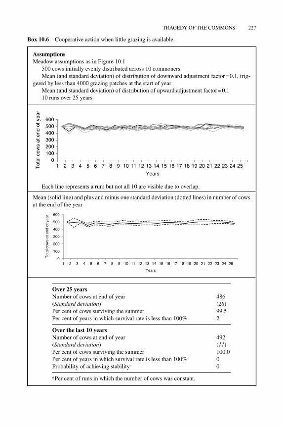
Assumptionsmeadow assumptions as in Figure 10.1
500 cows initially evenly distributed across 10 commonersmean (and standard deviation) of distribution of downward adjustment factor = 0.1, trig-
gered by less than 4000 grazing patches at the start of yearmean (and standard deviation) of distribution of upward adjustment factor = 0.110 runs over 25 years
0100200300400500600
1 2 3 4 5 6 7 8 9 10 11 12 13 14 15 16 17 18 19 20 21 22 23 24 25Tot
al c
ows
at e
nd o
f yea
r
Years
Each line represents a run: but not all 10 are visible due to overlap.
mean (solid line) and plus and minus one standard deviation (dotted lines) in number of cows at the end of the year
0
100
200
300
400
500
600
1 2 3 4 5 6 7 8 9 10 11 12 13 14 15 16 17 18 19 20 21 22 23 24 25
Tot
al c
ows
at e
nd o
f yea
r
Years
Over 25 yearsNumber of cows at end of year 486(Standard deviation) (28)Per cent of cows surviving the summer 99.5Per cent of years in which survival rate is less than 100% 2
Over the last 10 yearsNumber of cows at end of year 492(Standard deviation) (11)Per cent of cows surviving the summer 100.0Per cent of years in which survival rate is less than 100% 0Probability of achieving stabilitya 0
a Per cent of runs in which the number of cows was constant.
Box 10.6 Cooperative action when little grazing is available.

228 AGENT-BASEd mOdEllING IN ECONOmICS
we start each commoner with 50 cows and assume that both adjustment factors are distributed with a mean (and standard deviation) of 0.1. So, for example, if a commoner grazed 60 last year and there are less than 4000 grazing patches available at the start of this year and his downward adjustment factor is 0.1, then he will graze 54; but if there are 4000 or more grazing patches, he will increase his stock by 10% to 66%. At the macro level, although complete stability is not achieved, a large number of cows are supported, and there is a very high survival rate as shown in Box 10.6. But at the micro level, after 25 years, there is much more diversity between com-moners in the sizes of their grazing herds than if there was simply a limit of 50 or 60 cows per commoner set. In this example, after 25 years, one commoner has on average 31% (sd 8) of the cows on the meadow.
Other scenarios are suggested in the ‘Things to try’ sections. Alternatively, readers may like to explore Sugarscape, a well‐known agent‐based model in which agents move across a landscape consuming its resources (Epstein & Axtell, 1996). Parts of the Sugarscape model are available in the Netlogo library (li & Wilensky, 2009).
Our model does not explain how cooperation is attained. While case studies have shown what factors contribute to long‐term cooperative solutions, how such solutions have emerged is not clear. Exploring this, perhaps using variations of the repeated prisoner’s dilemma game, may prove interesting. (There are examples of a multi‐person iterated prisoner dilemma game in the Netlogo library (Wilensky, 2002).)
Returning to the themes of the book – interaction, heterogeneity and dynamics, this chapter has demonstrated the importance of combining all three. The commoners interact with their envi-ronment and, indirectly, with each other over time, and they are heterogeneous in that they react to changes in different ways. Agent‐based modelling facilitates the modelling of this complex dynamic system in a way that other methods simply cannot.
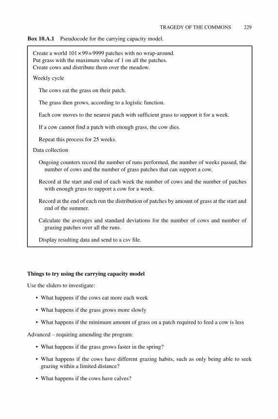
Appendix 10.A How to do it
Carrying capacity model
Purpose: The aim of the model is to establish the carrying capacity of a meadow.
Entities: Agents are cows and the patches carry grass.Stochastic processes: distribution of cows over the meadow.Initialisation:
• The initial number of cows
• How much each cow eats each week
• The weekly rate at which grass grows
• The minimum amount of grass on a patch required to feed a cow for a week
• The number of runs required
Outputs: data on the amount of grass and the number of cows is collected and sent to a csv file.
The pseudocode is in Box 10.A.1 and a screenshot in Figure 10.A.1. For the full code, see the website: Chapter 10 – Carrying Capacity Model.
TRAGEdy OF THE COmmONS 229
Things to try using the carrying capacity model
Use the sliders to investigate:
• What happens if the cows eat more each week
• What happens if the grass grows more slowly
• What happens if the minimum amount of grass on a patch required to feed a cow is less
Advanced – requiring amending the program:
• What happens if the grass grows faster in the spring?
• What happens if the cows have different grazing habits, such as only being able to seek grazing within a limited distance?
• What happens if the cows have calves?
Create a world 101 × 99 = 9999 patches with no wrap‐around.Put grass with the maximum value of 1 on all the patches.Create cows and distribute them over the meadow.
Weekly cycle
The cows eat the grass on their patch.
The grass then grows, according to a logistic function.
Each cow moves to the nearest patch with sufficient grass to support it for a week.
If a cow cannot find a patch with enough grass, the cow dies.
Repeat this process for 25 weeks.
data collection
Ongoing counters record the number of runs performed, the number of weeks passed, the number of cows and the number of grass patches that can support a cow.
Record at the start and end of each week the number of cows and the number of patches with enough grass to support a cow for a week.
Record at the end of each run the distribution of patches by amount of grass at the start and end of the summer.
Calculate the averages and standard deviations for the number of cows and number of grazing patches over all the runs.
display resulting data and send to a csv file.
Box 10.A.1 Pseudocode for the carrying capacity model.

230 AGENT-BASEd mOdEllING IN ECONOmICS
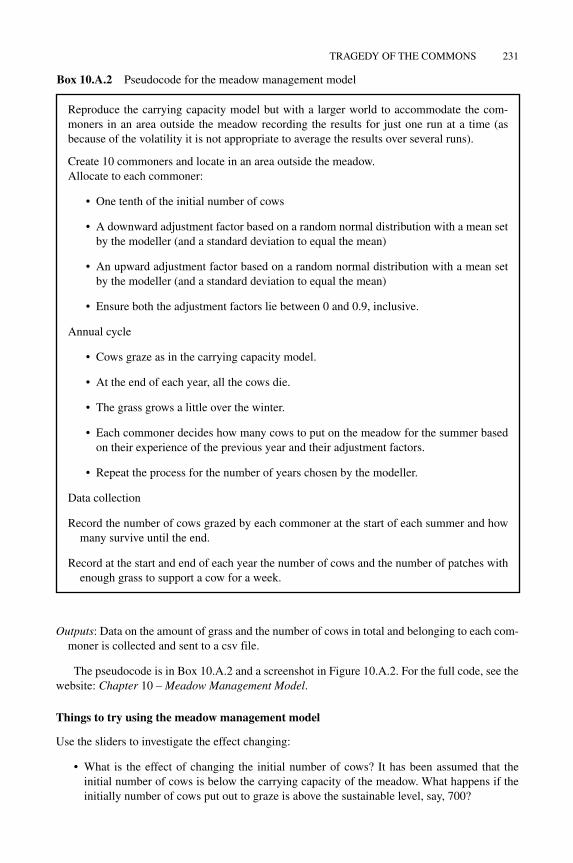
Meadow management model
Purpose: The aim of the model is to illustrate how a common area of grazing can be managed.Entities: The patches carry grass and there are two types of agents: cows and commoners.Stochastic processes:
• distribution of cows over the meadow
• Each commoner’s adjustment factors
• Allocation of cows to commoners
Initialisation:The meadow
• How much each cow eats every week
• The weekly rate at which grass grows
• The minimum amount of grass on a patch required to feed a cow
The commoners
• The initial number of cows
• The mean (and standard deviation) of the adjustment factors
• The number of years
Figure 10.A.1 Screenshot of the carrying capacity model.
TRAGEdy OF THE COmmONS 231
Outputs: data on the amount of grass and the number of cows in total and belonging to each com-moner is collected and sent to a csv file.
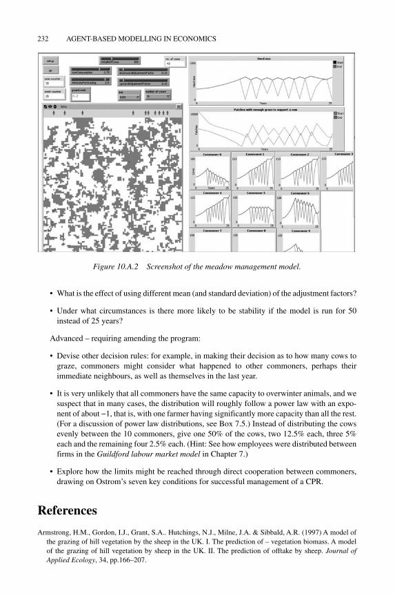
The pseudocode is in Box 10.A.2 and a screenshot in Figure 10.A.2. For the full code, see the website: Chapter 10 – Meadow Management Model.
Things to try using the meadow management model
Use the sliders to investigate the effect changing:
• What is the effect of changing the initial number of cows? It has been assumed that the initial number of cows is below the carrying capacity of the meadow. What happens if the initially number of cows put out to graze is above the sustainable level, say, 700?
Reproduce the carrying capacity model but with a larger world to accommodate the com-moners in an area outside the meadow recording the results for just one run at a time (as because of the volatility it is not appropriate to average the results over several runs).
Create 10 commoners and locate in an area outside the meadow.Allocate to each commoner:
• One tenth of the initial number of cows
• A downward adjustment factor based on a random normal distribution with a mean set by the modeller (and a standard deviation to equal the mean)
• An upward adjustment factor based on a random normal distribution with a mean set by the modeller (and a standard deviation to equal the mean)
• Ensure both the adjustment factors lie between 0 and 0.9, inclusive.
Annual cycle
• Cows graze as in the carrying capacity model.
• At the end of each year, all the cows die.
• The grass grows a little over the winter.
• Each commoner decides how many cows to put on the meadow for the summer based on their experience of the previous year and their adjustment factors.
• Repeat the process for the number of years chosen by the modeller.
data collection
Record the number of cows grazed by each commoner at the start of each summer and how many survive until the end.
Record at the start and end of each year the number of cows and the number of patches with enough grass to support a cow for a week.
Box 10.A.2 Pseudocode for the meadow management model
232 AGENT-BASEd mOdEllING IN ECONOmICS
• What is the effect of using different mean (and standard deviation) of the adjustment factors?
• Under what circumstances is there more likely to be stability if the model is run for 50 instead of 25 years?
Advanced – requiring amending the program:
• devise other decision rules: for example, in making their decision as to how many cows to graze, commoners might consider what happened to other commoners, perhaps their immediate neighbours, as well as themselves in the last year.
• It is very unlikely that all commoners have the same capacity to overwinter animals, and we suspect that in many cases, the distribution will roughly follow a power law with an expo-nent of about −1, that is, with one farmer having significantly more capacity than all the rest. (For a discussion of power law distributions, see Box 7.5.) Instead of distributing the cows evenly between the 10 commoners, give one 50% of the cows, two 12.5% each, three 5% each and the remaining four 2.5% each. (Hint: See how employees were distributed between firms in the Guildford labour market model in Chapter 7.)
• Explore how the limits might be reached through direct cooperation between commoners, drawing on Ostrom’s seven key conditions for successful management of a CPR.
References
Armstrong, H.m., Gordon, I.J., Grant, S.A.. Hutchings, N.J., milne, J.A. & Sibbald, A.R. (1997) A model of the grazing of hill vegetation by the sheep in the UK. I. The prediction of – vegetation biomass. A model of the grazing of hill vegetation by sheep in the UK. II. The prediction of offtake by sheep. Journal of Applied Ecology, 34, pp.166–207.
Figure 10.A.2 Screenshot of the meadow management model.

TRAGEdy OF THE COmmONS 233
Begg, d., Vernasca, G., Fischer, S. & dornbusch, R. (2011) Economics. Tenth Edition. london: mcGraw‐Hill Higher Education.
Chapman, d.S., Termansen, m., Quinn, C.H., Jin, N., Bonn, A., Cornell, S.J., Fraser, E.d.G., Hubacek, K., Kunin, W. E. & Reed, m.S. (2009) modelling the coupled dynamics of moorland management and upland vegetation. Journal of Applied Ecology, 46, pp.278–288 [Online]. Available at: http://onlinelibrary.wiley.com/doi/10.1111/j.1365‐2664.2009.01618.x/full [Accessed 29 September 2014].
dEFRA (2014) Common land: management, protection and registering to use. [Online]. Available at: https://www.gov.uk/common‐land‐management‐protection‐and‐registering‐to‐use [Accessed 29 September 2014].
EBlEX (2013) Planning Grazing Strategies for Better Returns. Agriculture and Horticulture development Board, Kenilworth [Online]. Available at: http://www.eblex.org.uk [Accessed 11 September 2014].
Epstein, J. & Axtell, R. (1996) Growing Artificial Societies: Social Science from the Bottom Up. Washington, dC: Brookings Institution Press.
Hardin, G. (1968) The Tragedy of the Commons. Science, 162, pp.243–1248.
Kahneman d. & Tversky, A. (1979) Prospect theory: An analysis of decision under risk. Econometrica, 47(2), pp.263–292.
li, J. and Wilensky, U. (2009). NetLogo Sugarscape 1 Immediate Growback model. http://ccl.northwestern.edu/netlogo/models/Sugarscape1ImmediateGrowback and NetLogo Sugarscape 2 Constant Growback model Center for Connected learning and Computer‐Based modeling, Northwestern University, Evanston, Il [Online]. Available at: http://ccl.northwestern.edu/netlogo/models/Sugarscape2ConstantGrowback. [Accessed 10 August 2014].
liu, J., dietz, T., Carpenter, S., Alberti, m., Carl Folke, C., moran, E., Pell, A., deadman, P., Kratz, T., lubchenco, J., Ostrom, E., Ouyang, Z., Provencher, W., Redman, C., Schneider, S. & Taylor, W. (2007); Complexity of coupled human and natural systems. Science, 317, pp.1513–1516.
Natural England (2014) Common Land [Online]. Available at: http://www.naturalengland.org.uk/ourwork/landscape/protection/historiccultural/commonland/ [Accessed 10 August 2014].
Ostrom, E. (1990) Governing the Commons. Cambridge, mA: Cambridge University Press.
Perman, R. ma, y., mcGilvray, J. & Common, m. (2003) Natural Resource and Environmental Economics. Harlow: Pearson.
Schindler, J. (2012a) Rethinking the tragedy of the commons: The integration of socio‐psychological disposi-tions. Journal of Artificial Societies and Social Simulation, 15(1), 4 [Online]. Available at: http://jasss.soc.surrey.ac.uk/15/1/4.html [Accessed 5 August 2014].
Schindler, J. (2012b) A simple agent‐based model of the tragedy of the commons. In: Troitzsch, K., möhring, m. & lotzmann, U., eds, Proceedings 26th European Conference on Modelling and Simulation. dudweiler: European Council for modelling and Simulation [Online]. Available at: http://www.openabm.org/files/models/3051/v1/doc/Article‐Conf‐Proceedings.pdf [Accessed 5 August 2014].
Straughton, E.A. (2008) Common Grazing in the Northern English Uplands, 1800–1965. lewiston, New york: Edwin mellon Press.
Strogatz, S. (1994) Nonlinear Dynamics and Chaos. Cambridge, mA: Westview.
Varian, H. (2010) Intermediate Microeconomics. Princeton: Princeton University Press.
Wilensky, U. (2002) NetLogo PD N‐Person Iterated model. Center for Connected learning and Computer‐Based modeling, Northwestern University, Evanston, Il [Online]. Available at: http://ccl.northwestern.edu/netlogo/models/PdN‐PersonIterated [Accessed 3 January 2015].