transfer matrix analysis - ethesisethesis.nitrkl.ac.in/105/1/10401015.pdf · transfer matrix method...
TRANSCRIPT
Transfer Matrix Analysis
A Project Submitted
In Partial Fulfillment of the Requirements
For the Degree of
Bachelor of Technology
In Civil Engineering
By
Jasmeet Singh
10401015&
Suman Samal10401020
DEPARTMENT OF CIVIL ENGINEERING
NATIONAL INSTITUTE OF TECHNOLOGY, ROURKELA2008

ii
Transfer Matrix Analysis
A Project Submitted
In Partial Fulfillment of the Requirements
For the Degree of
Bachelor of Technology
In Civil Engineering
By
Jasmeet Singh10401015
&
Suman Samal10401020
Under the Guidance of
Dr. M. R. Barik
DEPARTMENT OF CIVIL ENGINEERING
NATIONAL INSTITUTE OF TECHNOLOGY, ROURKELA 2008

iii
NATIONAL INSTITUTE OF TECHNOLOGY
ROURKELA
CERTIFICATE
This is to certify that the thesis entitled, “TRANSFER MATRIX ANALYSIS” submitted by
Jasmeet Singh (10401015) and Suman Samal (10401020) in partial fulfillment of the
requirements for the award of Bachelor of Technology Degree in Civil Engineering at the
National Institute of Technology, Rourkela (Deemed University) is an authentic work carried out
by them under my supervision and guidance.
Date:- Dr.M.R.Barik
Dept. of Civil Engineering
National Institute of Technology
Rourkela - 769008

iv
ACKNOWLEDGEMENT
We would like to articulate our deep gratitude to our project guide Dr. M.R.Barik who has
always been our motivation for carrying out the project.
We wish to convey our sincere gratitude to all the faculties of Civil Engineering Department who
have enlightened us during our studies. The facilities and co-operation received from the
technical staff of Civil Engineering Department is thankfully acknowledged.
We would like to thank the computer lab in charge M.tech. students for their timely inputs and
fulsome support. Last, but certainly not the least, we wish to thank our friends who stood beside
through all our endeavors.
Jasmeet Singh Suman Samal
Roll no.:-10401015 Roll no.:-10401020
Dept. of Civil Engineering Dept. of Civil Engineering
National Institute of Technology National Institute of Technology
Rourkela – 769008 Rourkela - 769008
v
CONTENTS
CHAPTER NO. TITLE PAGE NO.
CERTIFICATE iii
ACKNOWLEDGEMENT iv
CONTENTS v
LIST OF FIGURES viii
ABSTRACT x
1 INTRODUCTION 1
2 BASIC PRINCIPLE OF MATRIX METHOD 3 2.1 INTRODUCTION 4
2.2 MATRIX ADDITION AND SUBTRACTION 5
2.3 MATRIX MULTIPLICATION 5
2.4 TRANSPOSE OF A MATRIX 5
2.5 DETERMINANT OF A MATRIX 6
2.6 INVERSE OF A MATRIX 6
2.7 SOLVING A SYSTEM OF EQUATIONS USING MATRIX 7
2.7.1 Inverse Matrix Method 8
2.7.2 Cramer's Rule 9
3 TRANSFER MATRIX METHOD 10 3.1 ALGORITHM OF TRANSFER MATRIX METHOD 11
3.2 STATIC ANALYSIS 11
4 VIBRATIONS AND NATURAL FREQUENCY 16 4.1 INTRODUCTION 17
vi
4.2 DYNAMIC LOAD AND D’ALEMBERT PRINCIPLE 18
4.2.1 Modes of Vibration 19
4.3 DETERMINATION OF THE FUNDAMENTAL
FREQUENCY OF A MULTISTOREYED BUILDING 20
5 TORSIONAL VIBRATION OF SHAFTS 22 5.1 INTRODUCTION 23
5.2 SOLVING USING TRANSFER MATRIX METHOD 23
6 COMPUTER PROGRAMMING AND RESULTS 25 6.1 FUNDAMENTAL FREQUENCY OF SINGLE BAY
MULTI-STOREY BUILDING
6.1.1 Program 26
6.1.2 Flowchart 28
6.1.3 Result 29
6.2 FUNDAMENTAL FREQUENCY OF MULTIPE BAY
MULTIPLE-STOREY BUILDING
6.2.1 Program 30
6.2.2 Flowchart 33
6.2.3 Result 34
6.3 TORSIONAL VIBRATION OF SHAFT
6.3.1 Program 35
6.3.2 Flowchart 38
6.3.3 Result 39
6.4. ANALYSIS OF A BEAM SECTION
6.4.1 Program 40
6.4.2 Flowchart 51
6.4.3 Result 55
6.5. ANALYSIS OF A BEAM SECTION WITH UNEQUAL
SECTIONS AND WITH STIFFNERS
6.5.1 Program 56

vii
6.5.2 Flowchart 71
6.5.3 Result 75
7 CONCLUSION 76
viii
LIST OF FIGURES
SL No. Title Page No.
Fig.4.1 Modes of Vibration in Building 19
Fig.4.2 Modes of Vibration in String 20
Fig.4.3 Wind Load on Multi-Storeyed Building 20
Fig.5.1 Torsional Vibration of Shaft 24
Fig.6.1 Flowchart for calculating the Fundamental
Frequency of a Multi-Storeyed Building 28
Fig.6.2 Problem Statement 29
Fig.6.3 Solution obtained from Program 29
Fig.6.4 Flowchart for calculating the Fundamental
Frequency of a Multi-Storeyed Building
with Multiple Bays 33
Fig.6.5 Problem Statement 34
Fig.6.6 Solution obtained from Program 34
Fig 6.7 Flowchart for calculating the Fundamental
Frequency of a shaft with torsional forces
acting on it 38
Fig.6.8 Problem Statement 39
Fig.6.9 Solution obtained from Program 39
Fig 6.10 Flowchart for calculating the slope,
displacement, moment and reaction of a beam
section with a single cross-sectional area 51-54
Fig.6.11 Problem Statement 55
Fig.6.12 Solution obtained from Program 55
Fig 6.13 Flowchart for calculating the slope,

ix
displacement, moment and reaction of a beam
section with a various cross-sectional area and
having vertical and angular stiffeners 71-74
Fig.6.14. Problem Statement 75
Fig.6.15. Solution obtained from Program 75
x
NATIONAL INSTITUTE OF TECHNOLOGY
ROURKELA
ABSTRACT
Vibration analysis of arbitrary shaped structures has been of interest to structural designers for
several decades. Dynamic behavior of these structures is strongly dependent on boundary
conditions, geometrical shapes, material properties, different theories, and various complicating
effects. Closed-form solutions are possible only for a limited set of simple boundary conditions
and geometries. For analysis of arbitrary shaped structures, several numerical methods, such as
finite element method, finite difference method, boundary element method, and so on, are usually
applied. In this paper, we have tried to put some light on the methods of calculation of methods
to find out the vibration in structural members by taking advantages Transfer Matrix Methods in
calculating the vibration in Multi-Storied Buildings, the various beam actions in a given beam
with some given loading criteria and also used to compute the natural frequency of a shaft under
torsional vibration. Computer-Aided Analysis has also been provided to calculate the vibration in
a multi-storied building.

1
1
INTRODUCTION

2
Transfer matrix method is an approach to matrix structural analysis that uses a mixed
form of the element force-displacement relationship and transfers the structural behavior
parameters the joint forces and displacement from one end of the structures of line element to
other). An advantage of transfer matrix method is that it produces a system of equation to be
solved that are quite small in comparison with those produced by the stiffness method. A
disadvantage is the extensive sequence of operations that are required on a small matrix.
The transfer-matrix method is used when the total system can be broken into a sequence
of subsystems that interact only with adjacent subsystems. This method is suitable for line
structures such as arches and cables.
To implement the transfer matrix method, we need a relationship that gives the state of
forces and displacements at one end of the element in terms of force and displacement at the
other end.

3
2
BASIC PRINCIPLES OF MATRIX METHODS

4
2.1 INTRODUCTIONA matrix is defined as an ordered rectangular array of numbers. They can be used to
represent systems of linear equations, as will be explained below
Here are a couple of examples of different types of matrices:
• Symmetric matrix
• Diagonal matrix
• Upper Triangular matrix
• Lower Triangular matrix
• Zero matrix
• Identity matrix

5
And a fully expanded mxn matrix A, would look like this:
or in a more compact form:
2.2 MATRIX ADDITION AND SUBTRACTIONTwo matrices A and B can be added or subtracted if and only if their dimensions are the
same (i.e. both matrices have the identical amount of rows and columns.
2.3 MATRIX MULTIPLICATIONWhen the number of columns of the first matrix is the same as the number of rows in the
second matrix then matrix multiplication can be performed.
Where A has dimensions mxn, B has dimensions nxp. Then the product of A and B is the matrix
C, which has dimensions mxp. The ijth element of matrix C is found by multiplying the entries
of the ith row of A with the corresponding entries in the jth column of B and summing the n
terms
Note: That AxB is not the same as BxA
2.4 TRANSPOSE OF A MATRIXThe transpose of a matrix is found by exchanging rows for columns i.e. Matrix A = (aij)
and the transpose of A is:
AT=(aji) where j is the column number and i is the row number of matrix A.
In the case of a square matrix (m=n), the transpose can be used to check if a matrix is symmetric.
For a symmetric matrix A = AT

6
2.5 DETERMINANT OF A MATRIXDeterminants play an important role in finding the inverse of a matrix and also in solving
systems of linear equations. We assume we have a square matrix (m=n). The determinant of a
matrix A will be denoted by det(A) or |A|. Firstly the determinant of a 3x3 matrix will be
introduced then the nxn case will be shown.
Determinant of a 3x3 matrix
Determinant of a nxn matrix
For the general case, where A is an nxn matrix the determinant is given by:
Where the coefficients are given by the relation
where is the determinant of the (n-1) x (n-1) matrix that is obtained by deleting row i and
column j. This coefficient is also called the cofactor of aij.
2.6 INVERSE OF A MATRIXAssuming we have a square matrix A, which is non-singular ( i.e. det(A) does not equal
zero ), then there exists an nxn matrix A-1 which is called the inverse of A, such that this
property holds:
AA-1= A-1A = I where I is the identity matrix.
The inverse of a nxn matrix
The inverse of a general nxn matrix A can be found by using the following equation:

7
Where the adj(A) denotes the adjoint (or adjugate) of a matrix. It can be calculated by the
following method
• Given the nxn matrix A, define
to be the matrix whose coefficients are found by taking the determinant of the (n-1) x (n-
1) matrix obtained by deleting the ith row and jth column of A. The terms of B (i.e. B =
bij) are known as the cofactors of A.
• And define the matrix C, where
• The transpose of C (i.e CT) is called the adjoint of matrix A.
Lastly to find the inverse of A divide the matrix CT by the determinant of A to give its inverse.
2.7 SOLVING A SYSTEM OF EQUATIONS USING MATRIXA system of linear equations is a set of equations with n equations and n unknowns, is of
the form of
The unknowns are denoted by x1,x2,...xn and the coefficients (a's and b's above) are assumed to
be given. In matrix form the system of equations above can be written as:
A simplified way of writing above is like this ; Ax = b
After looking at this there are two methods used to solve matrices these are
8
• Inverse Matrix Method
• Cramer's Rule
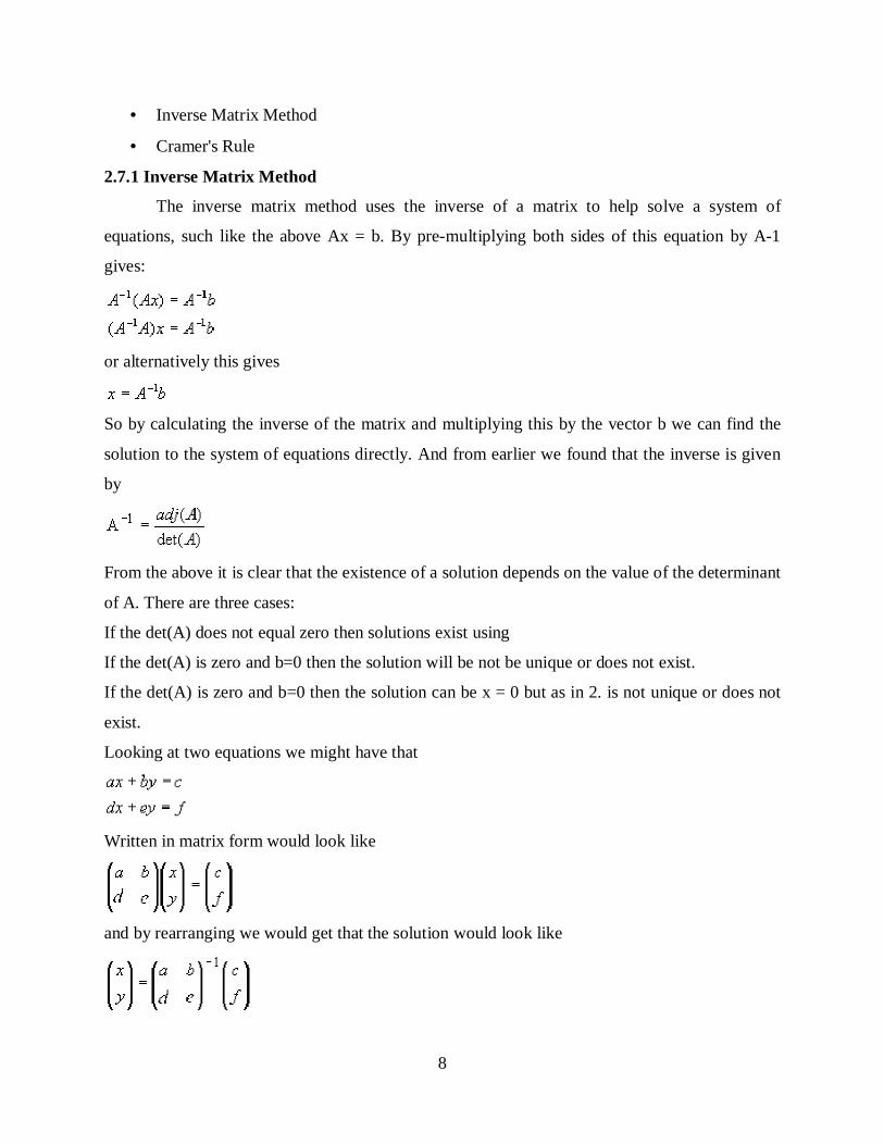
2.7.1 Inverse Matrix Method
The inverse matrix method uses the inverse of a matrix to help solve a system of
equations, such like the above Ax = b. By pre-multiplying both sides of this equation by A-1
gives:
or alternatively this gives
So by calculating the inverse of the matrix and multiplying this by the vector b we can find the
solution to the system of equations directly. And from earlier we found that the inverse is given
by
From the above it is clear that the existence of a solution depends on the value of the determinant
of A. There are three cases:
If the det(A) does not equal zero then solutions exist using
If the det(A) is zero and b=0 then the solution will be not be unique or does not exist.
If the det(A) is zero and b=0 then the solution can be x = 0 but as in 2. is not unique or does not
exist.
Looking at two equations we might have that
Written in matrix form would look like
and by rearranging we would get that the solution would look like
9
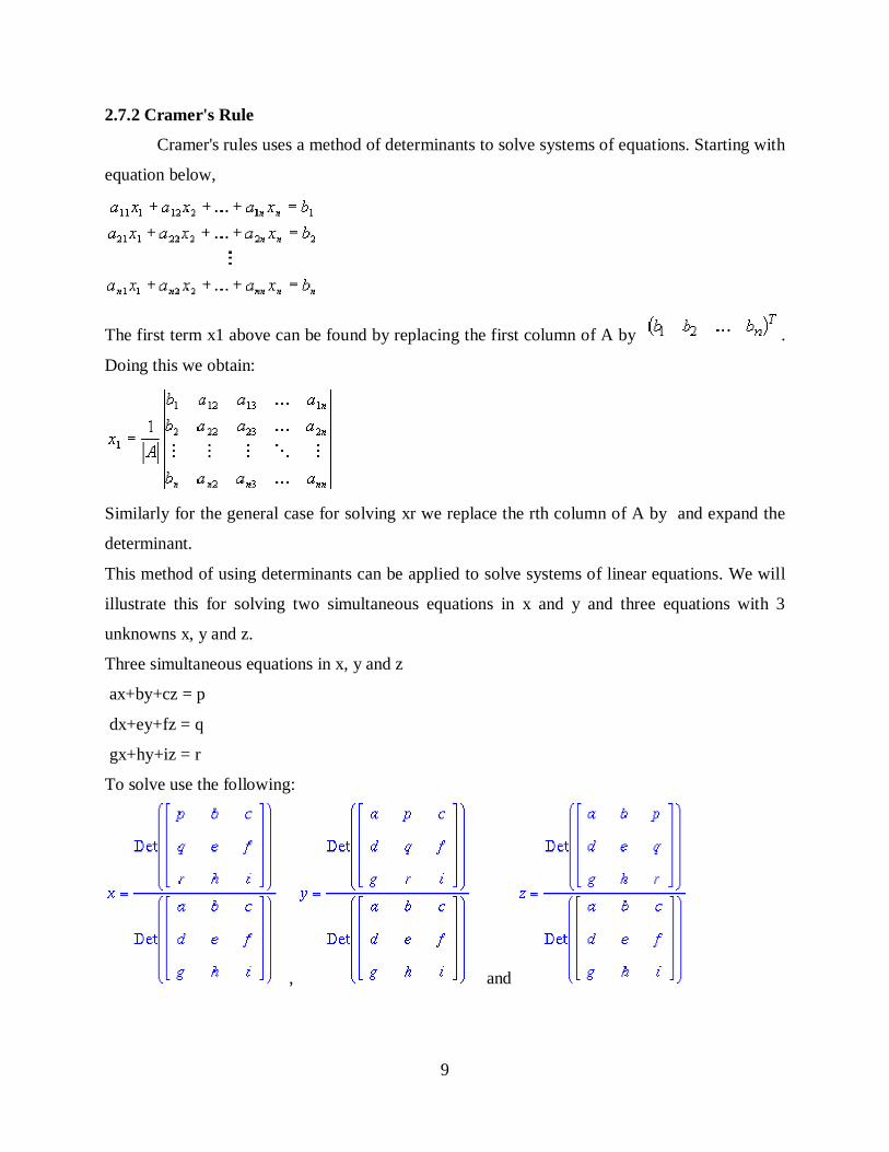
2.7.2 Cramer's Rule
Cramer's rules uses a method of determinants to solve systems of equations. Starting with
equation below,
The first term x1 above can be found by replacing the first column of A by .
Doing this we obtain:
Similarly for the general case for solving xr we replace the rth column of A by and expand the
determinant.
This method of using determinants can be applied to solve systems of linear equations. We will
illustrate this for solving two simultaneous equations in x and y and three equations with 3
unknowns x, y and z.
Three simultaneous equations in x, y and z
ax+by+cz = p
dx+ey+fz = q
gx+hy+iz = r
To solve use the following:
, and

10
3
TRANSFER MATRIX METHOD

11
3.1 ALGORITHM OF TRANSFER MATRIX METHOD The algorithm of the transfer matrix method is defined in two principal steps:-
1. The unknown initial parameter is defined by the matrix of initial parameters are transferred
using the matrix multiplication of transfer and nodal matrices into the end point of the applied
simulation. The boundary condition in the end point, implemented in the matrix of boundary
conditions, define the set of algebraic equations for determination of the unknown initial
parameters.
2. The calculated initial parameters are put into the state vector in initial point of
simulation and is repeated multiplications with transfer and nodal matrices determine the set of
resulting state vectors, stress and strain components in nodal points of the used discrete model.
3.2 STATIC ANALYSISThe state vector of bending components in the initial point of the arbitrary one-dimensional
element of the discrete simulation is given by:-
where vk, , Mk, Qk are the displacements, slope, moment and the lateral force in node K,
respectively. The last term of the vector k is the preliminary unit and has the importance for
incorporation of the external loading or deformation components into calculation process.
When deriving the corresponding transfer matrix BK, the known transformation
equations for the couplings of the components of the state vector kk between initial and end
points of the studied element can be written as
where lk is the length of the element and EJk is its stiffness.
12
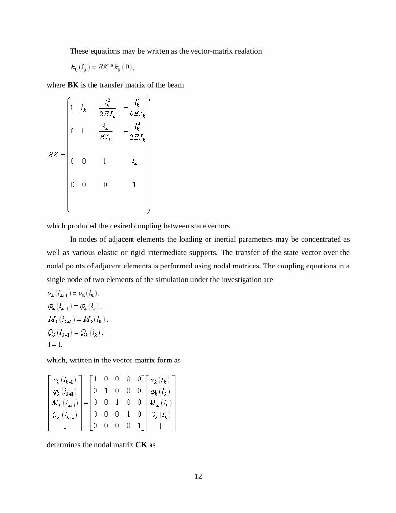
These equations may be written as the vector-matrix realation
where BK is the transfer matrix of the beam
which produced the desired coupling between state vectors.
In nodes of adjacent elements the loading or inertial parameters may be concentrated as
well as various elastic or rigid intermediate supports. The transfer of the state vector over the
nodal points of adjacent elements is performed using nodal matrices. The coupling equations in a
single node of two elements of the simulation under the investigation are
which, written in the vector-matrix form as
determines the nodal matrix CK as

13
When the node under investigation, a external force is present, the equation is
modified via
and the nodal matrix assumes form
with the nonzero force in the last column. Other external state components (initial deformation,
slope or moment) concentrated in this node may be incorporated into the last column of the nodal
matrix. If in addition the elastic support with stiffness characteristics Hk, hk is located in this
node
and the nodal matrix is given by
For the case of rigid support the stiffness characteristics Hk and hk tend to infinity (1020
and greater, depending on the type of computer).Hence, the degree of static redundancy of the
structure doesn’t influence the line algorithm of the solution. Generally, the significance of the
nodal matrix CK is the defined as

14
The nodal matrix, like the transfer matrix, allows the general variability of all transported
physical parameters in individual nodal points.
The boundary conditions defined in the initial point of the studied discrete simulation are
given by
where and are the unknown initial parameters.
The state vector k0 and the vector of the initial parameters u0 in the initial point of the
applied model are then given by
The relation between these two vectors is given by
k0=HL u0,
where HL is the matrix of initial parameters.
The matrix of initial parameters for the boundary conditions is then written as
The boundary conditions in the end point of the studied simulation

15
are implemented into the algorithm of method over the matrix of the boundary conditions RP,
derived similarly as HL, and expressed as
The algorithm of the TMM in a typical two-step concept is defined by two following
operations:
STEP 1- determination of the unknown initial parameters
STEP 2- input of calculated initial parameters into the initial state vector k0 and determination of
the state vectors in each node as
i.e.,
kn=(CK BK) kn-1
The present line concept may be adopted for the analysis of one-dimensional or multi-
dimensional structural simulations.
16
4
VIBRATIONS AND NATURAL FREQUENCY

17
4.1 INTRODUCTIONThe vibrating object is the source of the disturbance which moves through the medium. The
vibrating object which creates the disturbance could be the vocal chords of a person, the
vibrating string and sound board of a guitar or violin, the vibrating tines of a tuning fork, or the
vibrating diaphragm of a radio speaker. Any object which vibrates will create a sound. The
sound could be musical or it could be noisy; but regardless of its quality, the sound was created
by a vibrating object.
The fundamental tone, often referred to simply as the fundamental and abbreviated fo, is
the lowest frequency in a harmonic series.
The fundamental frequency (also called a natural frequency) of a periodic signal is the
inverse of the pitch period length. The pitch period is, in turn, the smallest repeating unit of a
signal. One pitch period thus describes the periodic signal completely. The significance of
defining the pitch period as the smallest repeating unit can be appreciated by noting that two or
more concatenated pitch periods form a repeating pattern in the signal. However, the
concatenated signal unit obviously contains redundant information.
A ‘fundamental bass’ is the root note, or lowest note or pitch in a chord or sonority when
that chord is in root position or normal form.
In terms of a superposition of sinusoids (for example, Fourier series), the fundamental
frequency is the lowest frequency sinusoidal in the sum.
To find the fundamental frequency of a sound wave in a tube that has a closed end you
will use the equation:
To find L you will use:
A key aspect of structural dynamic analysis concerns the behavior of a structure at
“resonance.” The natural frequency of vibration of a structure --- whether a wood-frame house or
a radio tower --- corresponds to that structure’s resonant frequency. If a structure is subjected to

18
vibration at its natural frequency, the displacements of that structure will reach a maximum
(“resonance”). The greater the displacements, greater is the stresses that are developed in the
framing members and connections of the structure.
The natural frequencies of vibration of a building depend on its mass and its stiffness (or
how flexible it is).
The natural frequency for each mode of vibration follows this rule:
f = natural frequency in Hertz.
K = the stiffness of the building associated with this mode
M = the mass of the building associated with this mode
Buildings tend to have lower natural frequencies when they are:
• Either heavier (more mass)
• Or more flexible (that is less stiff).
One of the main things that affect the stiffness of a building is its height. Taller buildings tend to
be more flexible, so they tend to have lower natural frequencies compared to shorter buildings.
4.2 DYNAMIC LOAD AND D’ALEMBERT PRINCIPLE
When we come to study vibrations, what we have is not static load but dynamic load. The very
nature of the load means that the response of the structure i.e the displacement, stress, reactions
etc. also varies with time.
The fundamental difference between static and dynamic loads is that acceleration of the body
must be taken into account. From Newton's Law, we know that any force produces acceleration,
however in statics we assumed that the load had been applied slowly and whatever effects were
19
to take place are over and the body is now in equilibrium. This cannot be assumed under
dynamic load.
The solution to this problem was proposed by D'Alembert who said that the acceleration can be
treated as another force acting opposite to the acceleration and of magnitude the mass times the
acceleration. This force is called the inertial force. The forces that act on the body can now be
treated as a set of forces in equilibrium.
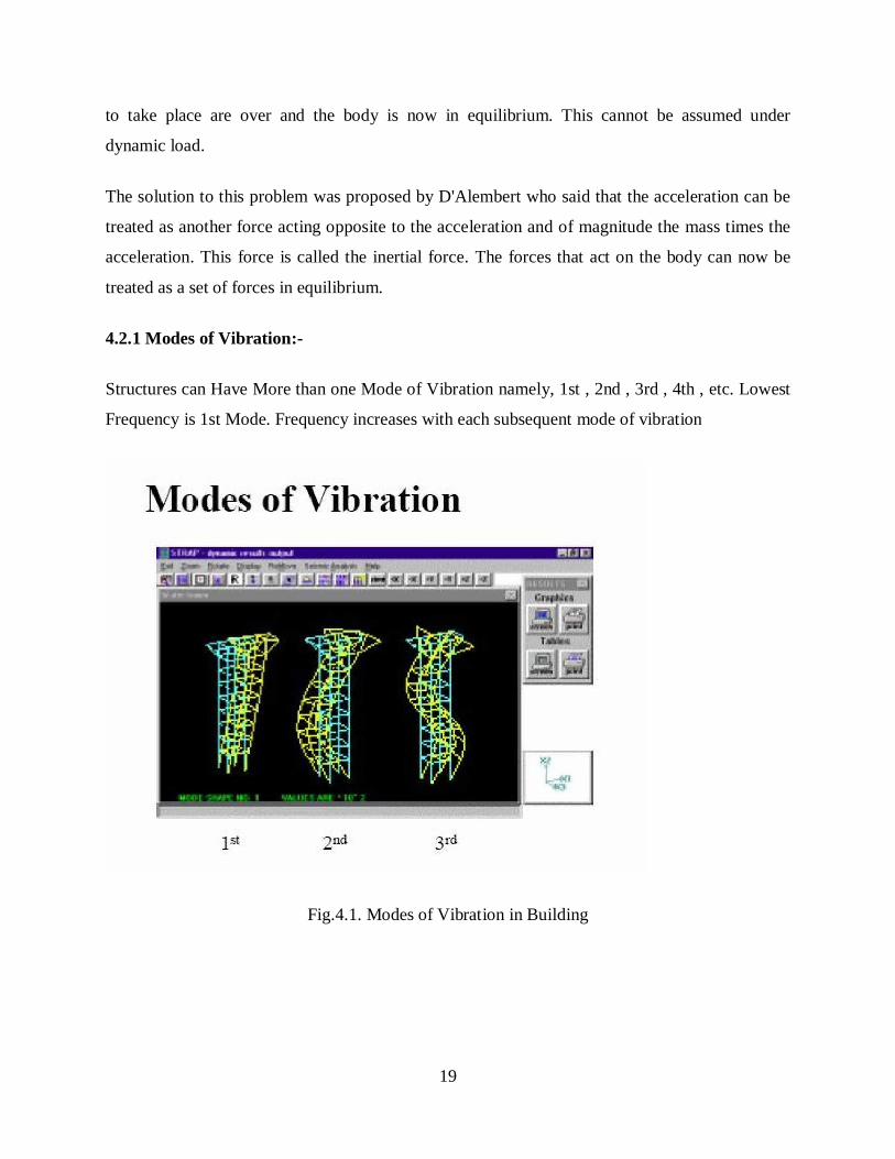
4.2.1 Modes of Vibration:-
Structures can Have More than one Mode of Vibration namely, 1st , 2nd , 3rd , 4th , etc. Lowest
Frequency is 1st Mode. Frequency increases with each subsequent mode of vibration
Fig.4.1. Modes of Vibration in Building
20
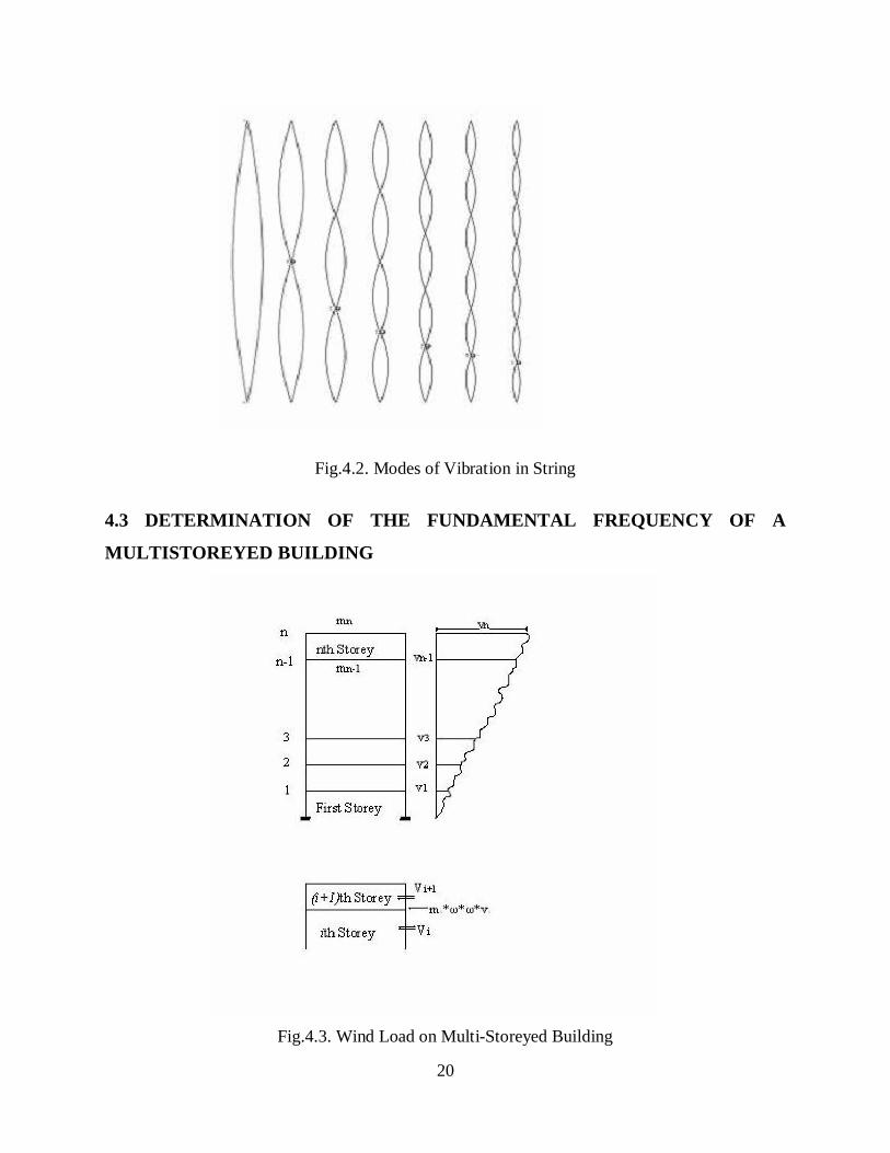
Fig.4.2. Modes of Vibration in String
4.3 DETERMINATION OF THE FUNDAMENTAL FREQUENCY OF A
MULTISTOREYED BUILDING
Fig.4.3. Wind Load on Multi-Storeyed Building
21
Consider a shear frame as shown consisting of n storey. Consider the free body diagram of the
ith storey. Here, m is the mass, K is the stiffness, V the shear, the frequency and v gives the
load displacements.
Initially, the displacement at the top storey level and the natural frequency are both assumed. By
using the transfer matrix method it is possible to find the displacement at the base as well as the
shear in the base storey. If the support displacement is not zero, a new value for the natural
frequency is assumed and the procedure is repeated till the value for the natural frequency is
assumed and the procedure is repeated till we get the value for the base displacement at the base
equal to zero.
Vi = Vi+1 + mi2vi
vi– vi-1= Vi/ki= (Vi+1 + mi2vi )/ki
22
5
TORSIONAL VIBRATION OF A SHAFT

23
5.1 INTRODUCTION
Torsional vibration is angular vibration of an object--commonly a shaft along its axis of
rotation. A ROTATING shaft can exhibit torsional vibration when, because the dynamic
coefficient of friction is less than the static value, the frictional force at the bearings supporting
the shaft decreases as the shaft begins to rotate. The torque in the shaft when it begins to turn is
greater than is required to overcome the running friction in the bearings, and the shaft accelerates
and may overrun the drive until the speed of the shaft is reduced to zero. Then superposed on the
steady rotation of the shaft there is a vibration of an amplitude such that the instantaneous
angular velocity of the shaft varies between zero and rather more than twice the mean value.
5.2 SOLVING USING TRANSFER MATRIX METHOD
Torsional vibration of the shaft can be solved by the transfer matrix method by applying the
following equation
1
11
0 1
R R
nn n
kT Tθ θ
−
=
2
1
1 01
R R
nn nJT Tθ θ
ω−
= −
where Jn=Rotary inertia of the rotor n
kn=stiffness of the shaft connecting (n-1) to n rotors.
n=Twist at rotor n

24
Fig.5.1. Torsional Vibration of Shaft
Combining we get
22 1
11
1
R Rn
nn nn
n
k
T TJJk
θ θ
ωω −
= − −

25
6
COMPUTER PROGRAMMING AND RESULTS

26
6.1 FUNDAMENTAL FREQUENCY OF SINGLE BAY MULTI-STOREY
BUILDING
6.1.1 Program
#include<iostream.h>
#include<conio.h>
void main()
{
double mass[10], stiffness[10], V[10], v[10], m=1.0, n=1.0;
int storey=0, i, j=0, k, l=0;
for(i=0;i<10;i++)
{
mass[i]=0.0;
stiffness[i]=0.0;
v[i]=0.0;
V[i]=0.0;
}
cout<<"ENTER THE NUMBER OF STOREYS: ";
cin>>storey;
for(i=1;i<=storey;i++)
{
cout<<"ENTER THE MASS OF BEAM IN STOREY "<<i<<" = ";
cin>>mass[i];
cout<<"ENTER THE STIFFNESS OF BEAM IN STOREY "<<i<<" = ";
cin>>stiffness[i];
}
V[storey+1]=0;
v[storey]=1;
for(i=0; i<500; i++)
{
j=0;

27
while (j<storey)
{
k=storey-j;
V[k]=(V[k+1])+(mass[k]*i*v[k]);
v[k-1]=((-1)*V[k+1]/stiffness[k])+v[k]-(mass[k]*i*v[k]/stiffness[k]);
j=j+1;
m=v[0];
}
if((n/m)<0)
cout<<i-1;
n=m;
}
}

28
6.1.2 Flowchart
Fig.6.1. Flowchart for calculating the Fundamental Frequency of a Multi-Storeyed Building

29
6.1.3 Result
Fig.6.2. Problem Statement
SOLUTION-
Natural Frequency=209 Hz
From Program
Fig.6.3. Solution obtained from Program

30
6.2 FUNDAMENTAL FREQUENCY OF MULTIPE BAY MULTIPLE-STOREY
BUILDING
6.2.1 Program
#include<iostream.h>
#include<conio.h>
void main()
{
double m[10][10], ks[10][10], mass[10], stiffness[10], V[10], v[10], p=1.0;
double n=1.0, tempm, tempk, tempmk, t;
int storey=0, bay=0, i, j=0, k, q, r;
for(i=1;i<=10;i++)
for(q=1;q<=10;q++)
{
m[i][q]=0.0;
ks[i][q]=0.0;
mass[i]=0.0;
stiffness[i]=0.0;
v[i]=0.0;
V[i]=0.0;
}
cout<<"ENTER THE NUMBER OF STOREYS: ";
cin>>storey;
cout<<"ENTER THE NUMBER OF BAYS: ";
cin>>bay;
for(i=1;i<=storey;i++)
for(q=1;q<=bay;q++)
{
cout<<"ENTER THE MASS OF BEAM IN STOREY "<<i<<" BAY
"<<q<<" = ";
cin>>m[i][q];

31
cout<<"ENTER THE STIFFNESS OF BEAM IN STOREY "<<i<<"
BAY "<<q<<" = ";
cin>>ks[i][q];
}
for(i=1;i<=storey;i++)
{
for(q=1;q<=bay;q++)
{
mass[i]=mass[i]+(m[i][q]/bay);
}
}
for(i=1;i<=storey;i++)
{
tempm=0.0;
tempk=1.0;
tempmk=0.0;
for(q=1;q<=bay;q++)
{
tempm=tempm+m[i][q];
/*cout<<"\n tempm = "<<tempm;*/
tempk=tempk*ks[i][q];
/*cout<<"\n tempk = "<<tempk;*/
t=1.0;
for(r=1;r<=bay;r++)
{
if(q!=r)
t=t*ks[i][r];
/*cout<<"\n ks="<<ks[i][r];
cout<<"\n t = "<<t;*/
}
tempmk=tempmk+(m[i][q]*t);
32
}
stiffness[i]=(tempk*tempm)/tempmk;
/*cout<<"stiffness"<<stiffness[i];*/
}
V[storey+1]=0;
v[storey]=1;
for(i=0; i<500; i++)
{
j=0;
while (j<storey)
{
k=storey-j;
V[k]=(V[k+1])+(mass[k]*i*v[k]);
v[k-1]=((-1)*V[k+1]/stiffness[k])+v[k]-(mass[k]*i*v[k]/stiffness[k]);
j=j+1;
p=v[0];
}
if((n/p)<0)
cout<<"THE NATURAL FREQUENCY "<<(i-1);
n=p;
}
}

33
6.2.2 Flowchart
Fig.6.4. Flowchart for calculating the Fundamental Frequency of a Multi-Storeyed Building with
Multiple Bays

34
6.2.3 Result
Fig.6.5. Problem Statement
SOLUTION-
Natural Frequency=209 Hz
From Program
Fig.6.6. Solution obtained from Program
35
6.3 TORSIONAL VIBRATION OF SHAFT
6.3.1 Program
#include<iostream.h>
#include<conio.h>
#include<math.h>
#include<stdio.h>
#include "nrutil.h"
#include "nrutil.c"
void matrix_mult( float **q1, float **q2, float **ans, int r1, int c1, int r2, int c2)
{
int i,j,k;
if(c1!=r2)
cout<<"\nTHE MATRIX MULTIPLICATION IS NOT POSSIBLE\n";
else
for(i=1;i<=r1;i++)
for(j=1;j<=c2;j++)
{
ans[i][j]=0;
for(k=1;k<=c1;k++)
ans[i][j]=ans[i][j]+(q1[i][k]*q2[k][j]);
}
}
void main()
{
double J[10], ks[10], Th[10], T[10], m=1.0, n=1.0, fin;
int rotor=0, i, j, w, f, k;
float **a, **b, **c;
a = matrix(1,2,1,2);
b = matrix(1,2,1,2);
c = matrix(1,2,1,2);

36
for(i=1;i<=10;i++)
{
J[i]=0.0;
ks[i]=0.0;
Th[i]=0.0;
T[i]=0.0;
}
cout<<"ENTER THE NUMBER OF ROTOR: ";
cin>>rotor;
for(i=1;i<=rotor;i++)
{
cout<<"THE ROTARY INERTIA OF ROTOR NO."<<i<<" = ";
cin>>J[i];
}
for(i=2;i<=rotor;i++)
{
cout<<"THE STIFFNESS OF SHAFT NO."<<i<<" = ";
cin>>ks[i];
}
for(w=10;w<=1000;w++)
{
a[1][1]=1.0;
a[1][2]=0.0;
a[2][1]=0.0;
a[2][2]=1.0;
for(i=rotor;i>=2;i--)
{
b[1][1]=1;
b[1][2]=1/ks[i];
b[2][1]=-1*w*w*J[i];

37
b[2][2]=1-(w*w*J[i]/ks[i]);
matrix_mult( a, b, c, 2, 2, 2, 2);
for(k=1;k<=2;k++)
for(j=1;j<=2;j++)
{
a[k][j]=c[k][j];
}
}
fin=(a[2][1]-a[2][2]*w*w*J[1])/10000;
/*cout<<"\n fin "<<w<<"="<<abs(fin);*/
if((abs(fin))<1)
cout<<"\n THE NATURAL FREQUENCY IS "<<w;
}
}

38
6.3.2 Flowchart
Fig 6.7. Flowchart for calculating the Fundamental Frequency of a shaft with torsional forces
acting on it

39
6.3.3 Result
Fig.6.8. Problem Statement
SOLUTION-
Natural Frequency-126 Hz
From Program
Fig.6.9. Solution obtained from Program

40
6.4 ANALYSIS OF A BEAM SECTION
6.4.1 Program
#include<iostream.h>
#include<conio.h>
#include<math.h>
#include "nrutil.h"
#include "nrutil.c"
struct uniform_load
{
float w, epoa, spoa;
};
uniform_load ul[10];
struct concentrated_load
{
float W, poa;
};
concentrated_load cl[10];
void matrix_multiplication( float **q1, float **q2, float *ans, int r1, int c1, int r2, int c2=1)
{
int i,j,k;
if(c1!=r2)
cout<<"\nTHE MATRIX MULTIPLICATION IS NOT POSSIBLE\n";
else
for(i=1;i<=r1;i++)
for(j=1;j<=c2;j++)
{
ans[i]=0;
for(k=1;k<=c1;k++)
ans[i]=ans[i]+(q1[i][k]*q2[k][j]);
}

41
}
void matrix_addition( float *q1, float *q2, float *ans, int r1, int c1, int r2, int c2=1)
{
int i,j;
if(r1!=r2 && c1!=c2)
cout<<"\nTHE MATRIX ADDITION IS NOT POSSIBLE\n";
else
for(i=1;i<=r1;i++)
ans[i]=q1[i]+q2[i];
}
float swappingrowsfn(float **mat, int row, int order)
{
float delement,tempvar;
int var=0;
for(int i=row;i<order;i++)
{
if(mat[i][row]!=0)
{
var=1;
for(int j=0;j<order;j++)
{
tempvar=mat[row][j];
mat[row][j]=mat[i][j];
mat[i][j]=tempvar;
}
}
if(var==1)
break;
}
42
delement=mat[row][row];cout<<"\n"<<delement;
return(delement);
}
void g_valfunc( float **g_val, float l, float ei)
{
int i,j;
for(i=1;i<=4;i++)
for(j=1;j<=4;j++)
g_val[i][j]=0.0;
g_val[1][1]=1.0;
g_val[1][2]=l;
g_val[1][3]=-1*l*l/(2*ei);
g_val[1][4]=-1*l*l*l/(6*ei);
g_val[2][2]=1.0;
g_val[2][3]=-1*l/(ei);
g_val[2][4]=-1*l*l/(2*ei);
g_val[3][3]=1.0;
g_val[3][4]=l;
g_val[4][4]=1.0;
}
void z_valfunc(float *z, float d, float s, float m, float r)
{
z[1]=d;
z[2]=s;
z[3]=m;
z[4]=r;
}
void z_valfuncforc(float **z, float w)
{
int i;
for(i=1;i<4;i++)

43
z[i][1]=0;
z[4][1]=-1.0*w;
}
void z_valfuncforu(float *z, float w, float l, float ei)
{
z[1]=w*l*l*l*l/(24*ei);
z[2]=w*l*l*l/(6*ei);
z[3]=-1.0*w*l*l/2;
z[4]=-1.0*w*l;
}
void main()
{
int flag1, i=0, j=0, k=1, bar=0, n, u=1, c=1, x, y, p, q, con=1, z, l, m;
char flag2='y';
float len, leng, length[10], EI[10], tl=0, ch, **Z, **G, *cons;
float **equa, **inv, **Zfor, answ, temp, *temp1, *constant;
for(i=1;i<=10;i++)
{
length[i]=0;
EI[i]=0;
}
while (flag2=='y' || flag2=='Y')
{
bar=bar+1;
cout<<"ENTER THE LENGTH: ";
cin>>length[bar];
length[bar]=length[bar]*1.0;
cout<<"ENTER THE VALUE OF EI: ";
cin>>EI[bar];
EI[bar]=EI[bar]*1.0;
cout<<"DO YOU WANT TO ENTER MORE (Y/N): ";

44
cin>>flag2;
}
for(i=1;i<=10;i++)
tl=tl+length[i];
n=bar+1;
flag2='y';
cout<<" :ENTER THE LOAD DETAILS:";
while (flag2=='y' || flag2=='Y')
{
cout<<"\n ENTER YOUR PREFERENCE: \n";
cout<<"1 FOR UDL \n2 FOR POINT LOAD: ";
cin>>flag1;
switch(flag1)
{
case(1): cout<<"ENTER THE UNIFORM LOAD: ";
cin>>ul[u].w;
cout<<"ENTER THE STARTING POINT OF
APPLICATION: ";
cin>>ul[u].spoa;
cout<<"ENTER THE END POINT OF
APPLICATION: ";
cin>>ul[u].epoa;
u=u+1;
break;
case(2): cout<<"ENTER THE LOAD: ";
cin>>cl[c].W;
cout<<"ENTER THE POINT OF APPLICATION:
";
cin>>cl[c].poa;
c=c+1;
break;

45
default: cout<<"WRONG OPTION";
break;
}
cout<<"DO YOU WANT TO ENTER MORE (Y/N): ";
cin>>flag2;
}
Z = matrix(0,bar,1,4);
equa = matrix(1,n,1,n);
inv = matrix(1,n,1,n);
G = matrix(1,4,1,4);
cons = vector(1,n);
temp1 = vector(1,4);
Zfor = matrix(1,4,1,1);
constant = vector(1,4);
for(i=1; i<=n; i++)
for(j=0; j<=n; j++)
equa[i][j]=0.0;
cout<<"ENTER 1 IF THE STARTING POINT IS SIMPLY SUPPORTED\n";
cout<<"ENTER 2 IF THE STARTING POINT IS FIXED\n";
cin>>flag1;
switch(flag1)
{
case(1): z_valfunc(Z[0], 0, 1, 0, 1);
break;
case(2): z_valfunc(Z[0], 0, 0, 1, 1);
break;
default: cout<<"WRONG OPTION";
}
cout<<"ENTER 1 IF THE END POINT IS SIMPLY SUPPORTED\n";
cout<<"ENTER 2 IF THE END POINT IS FIXED\n";
cin>>flag1;

46
switch(flag1)
{
case(1): z_valfunc(Z[bar], 0, 1, 0, 1);
break;
case(2): z_valfunc(Z[bar], 0, 0, 1, 1);
break;
default: cout<<"WRONG OPTION";
}
p=0;
for(i=1;i<bar;i++)
z_valfunc(Z[i], 0, 0, 0, 1);
for(i=1;i<=bar;i++)
{
leng=0.0;
j=1;
k=1;
for(m=1;m<=4;m++)
constant[m]=0.0;
for(m=1;m<=i;m++)
leng=leng+length[m];
while (leng>ul[j].spoa)
{
if(leng>ul[j].epoa)
len=ul[j].epoa-ul[j].spoa;
else
len=leng-ul[j].spoa;
z_valfuncforu(temp1, ul[j].w, len, EI[i]);
matrix_addition(temp1, constant, constant, 4, 1, 4, 1);
j++;
/*for(m=1;m<=4;m++)
cout<<"\n CONS["<<m<<"]="<<constant[m];*/

47
}
while (leng>cl[k].poa)
{
len=leng-cl[k].poa;
g_valfunc(G, len, EI[i]);
z_valfuncforc(Zfor, cl[k].W);
matrix_multiplication(G, Zfor, temp1, 4, 4, 4, 1);
matrix_addition(temp1, constant, constant, 4, 1, 4, 1);
k++;
/*for(m=1;m<=4;m++)
cout<<"\n CONS["<<m<<"]="<<constant[m];*/
}
x=1;
do
{
if(Z[i][x]==0.0)
{
cons[con]=-1*constant[x];
con++;
}
x++;
}
while (i==bar && x<=4);
/*for(m=1;m<=n;m++)
cout<<"\n CONS["<<m<<"]="<<cons[m];*/
for(l=i; l>=1; l--)
{
len=0;
for(m=1; m<=l; m++)
len=len+length[m];
48
g_valfunc(G, len, EI[l]);
for(m=1; m<=4; m++)
temp1[m]=Z[i-l][m];
x=1;
do
{
if (Z[i][x]==0)
{
q=0;
p++;
for(y=1; y<=4; y++)
{
if (temp1[y]!=0)
{
q++;
if (p<=n)
equa[p][q]=G[x][y];
else
if (p>n)
equa[p+q-n][n]=G[x][y];
}
}
}
x++;
}
while (i==bar && x<=4);
}
}
/*for(i=1;i<=n;i++)
for(j=1;j<=n;j++)
cout<<"\n eq["<<i<<"]["<<j<<"]="<<equa[i][j];*/
49
for(x=1; x<=n; x++)
for(y=1; y<=n; y++)
inv[x][y]=0.0;
for(x=1; x<=n; x++)
inv[x][x]=1.0;
for(x=1; x<=n; x++)
{
temp=equa[x][x];
if(equa[x][x]==0)
temp=swappingrowsfn(equa,x,n);
if(temp==0)
break;
for(y=1; y<=n; y++)
{
equa[x][y]= (equa[x][y])/temp;
inv[x][y]= (inv[x][y])/temp;
}
for(y=1; y<=n; y++)
{
if (y!=x)
{
temp=equa[y][x];
for(z=1; z<=n; z++)
{
equa[y][z]=equa[y][z]-temp*equa[x][z];
inv[y][z]=inv[y][z]-temp*inv[x][z];
}
}
}
}
if(temp==1)

50
cout<<"\nThe solution does not exist.";
for(i=1; i<=n; i++)
{
answ=0.0;
for(j=1; j<=n; j++)
answ= answ + ((inv[i][j])*(cons[j]));
cout<<"\nTHE ANSWER IS: "<<answ;
}
}

51
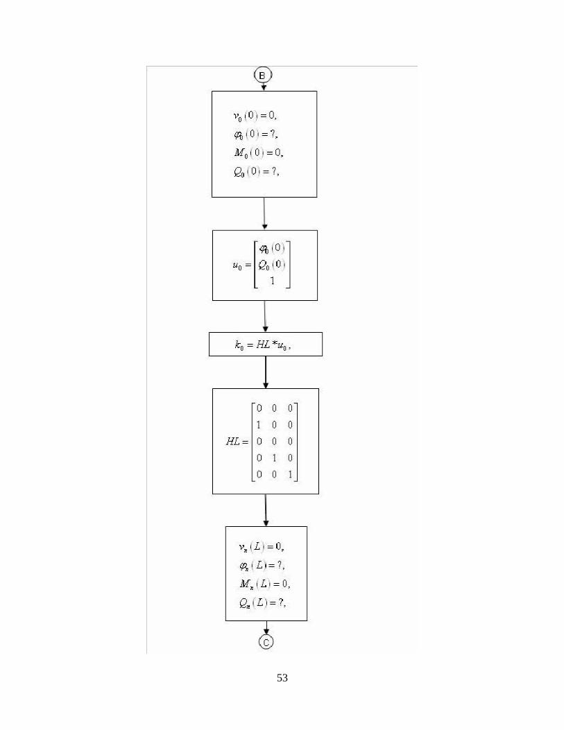
6.4.2 Flowchart

52
53
54
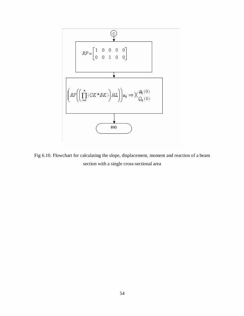
Fig 6.10. Flowchart for calculating the slope, displacement, moment and reaction of a beam
section with a single cross-sectional area
55
6.4.3 Result
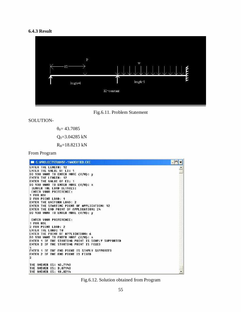
Fig.6.11. Problem Statement
SOLUTION-
0= 43.7085
Q0=3.04285 kN
RB=18.8213 kN
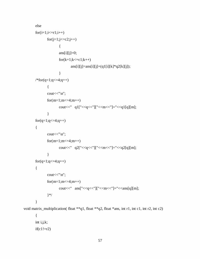
From Program
Fig.6.12. Solution obtained from Program

56
6.5 ANALYSIS OF A BEAM SECTION WITH UNEQUAL SECTIONS AND
WITH STIFFNERS
6.5.1 Program
#include<iostream.h>
#include<conio.h>
#include<math.h>
#include "nrutil.h"
#include "nrutil.c"
int n;
float length[10], EI[10], tl=0;
struct uniform_load
{
float w, epoa, spoa;
};
uniform_load ul[10];
struct concentrated_load
{
float W, poa;
};
concentrated_load cl[10];
struct support_constraints
{
float Hk, hk;
};
support_constraints sc[10];
void matrix_mult( float **q1, float **q2, float **ans, int r1, int c1, int r2, int c2)
{
int i,j,k,q,m;
if(c1!=r2)
cout<<"\nTHE MATRIX MULTIPLICATION IS NOT POSSIBLE\n";
57
else
for(i=1;i<=r1;i++)
for(j=1;j<=c2;j++)
{
ans[i][j]=0;
for(k=1;k<=c1;k++)
ans[i][j]=ans[i][j]+(q1[i][k]*q2[k][j]);
}
/*for(q=1;q<=4;q++)
{
cout<<"\n";
for(m=1;m<=4;m++)
cout<<" q1["<<q<<"]["<<m<<"]="<<q1[q][m];
}
for(q=1;q<=4;q++)
{
cout<<"\n";
for(m=1;m<=4;m++)
cout<<" q2["<<q<<"]["<<m<<"]="<<q2[q][m];
}
for(q=1;q<=4;q++)
{
cout<<"\n";
for(m=1;m<=4;m++)
cout<<" ans["<<q<<"]["<<m<<"]="<<ans[q][m];
}*/
}
void matrix_multiplication( float **q1, float **q2, float *ans, int r1, int c1, int r2, int c2)
{
int i,j,k;
if(c1!=r2)

58
cout<<"\nTHE MATRIX MULTIPLICATION IS NOT POSSIBLE\n";
else
for(i=1;i<=r1;i++)
for(j=1;j<=c2;j++)
{
ans[i]=0;
for(k=1;k<=c1;k++)
ans[i]=ans[i]+(q1[i][k]*q2[k][j]);
}
}
void matrix_addition( float *q1, float *q2, float *ans, int r1, int c1, int r2, int c2=1)
{
int i;
if(r1!=r2 && c1!=c2)
cout<<"\nTHE MATRIX ADDITION IS NOT POSSIBLE\n";
else
for(i=1;i<=r1;i++)
ans[i]=q1[i]+q2[i];
}
void g_valfunction(float **g_val, float l, float ei)
{
int i,j;
for(i=1;i<=4;i++)
for(j=1;j<=4;j++)
g_val[i][j]=0.0;
g_val[1][1]=1.0;
g_val[1][2]=l;
g_val[1][3]=-1*l*l/(2*ei);
g_val[1][4]=-1*l*l*l/(6*ei);
g_val[2][2]=1.0;
59
g_val[2][3]=-1*l/(ei);
g_val[2][4]=-1*l*l/(2*ei);
g_val[3][3]=1.0;
g_val[3][4]=l;
g_val[4][4]=1.0;
}
void g_valfunc(float **gvalf, float ep, float sp)
{
int i, j, k, m, l, flag=0;
float len=0, leng=0, temp, le;
float **gv,**gv1,**gv2;
gv = matrix(1,4,1,4);
gv1 = matrix(1,4,1,4);
gv2 = matrix(1,4,1,4);
for(i=1;i<=4;i++)
for(j=1;j<=4;j++)
{
gvalf[i][j]=0.0;
gv[i][j]=0.0;
gv1[i][j]=0.0;
gv2[i][j]=0.0;
}
for(i=1;i<=4;i++)
{
gvalf[i][i]=1.0;
gv[i][i]=1.0;
gv1[i][i]=1.0;
gv2[i][i]=1.0;
}
for(i=1; i<n; i++)
{
60
len=len+length[i];
if(sp==len)
{
/*cout<<"\n i"<<i;*/
for(l=i; l>0; l--)
{
if(ep<(len-length[l]))
{
gv2[3][2]=sc[l].Hk;
gv2[4][1]=sc[l].hk;
le=length[l];
/*cout<<"l"<<l<<"ep"<<ep<<"sp"<<sp<<"len"<<len<<"le"<<le<<"length"<<length[l-
1];*/
g_valfunction(gv, le, EI[l]);
for(k=1;k<=4;k++)
for(m=1;m<=4;m++)
cout<<"\n
gv["<<k<<"]["<<m<<"]="<<gv[k][m];
matrix_mult(gv2, gv, gv1, 4, 4, 4, 4);
for(k=1;k<=4;k++)
for(m=1;m<=4;m++)
{
gv[k][m]=gv1[k][m];
/*cout<<"\n
gv["<<k<<"]["<<m<<"]="<<gv[k][m];*/
}
matrix_mult(gv, gvalf, gv1, 4, 4, 4, 4);
for(k=1;k<=4;k++)
for(m=1;m<=4;m++)
gvalf[k][m]=gv1[k][m];
61
}
else
if(flag==0)
{
for(k=1; k<=l; k++)
leng=leng+length[k];
temp=ep-leng;
gv2[3][2]=sc[l].Hk;
gv2[4][1]=sc[l].hk;
g_valfunction(gv, temp, EI[l]);
matrix_mult(gv2, gv, gv1, 4, 4, 4, 4);
for(k=1;k<=4;k++)
for(m=1;m<=4;m++)
gv[k][m]=gv1[k][m];
matrix_mult(gv, gvalf, gv1, 4, 4, 4, 4);
for(k=1;k<=4;k++)
for(m=1;m<=4;m++)
gvalf[k][m]=gv1[k][m];
flag=1;
}
}
}
}
}
void z_valfunc(float *z, float d, float s, float m, float r)
{
z[1]=d;
z[2]=s;
z[3]=m;
z[4]=r;
}

62
void z_valfuncforc(float **z, float w)
{
int i;
for(i=1;i<4;i++)
z[i][1]=0;
z[4][1]=-1.0*w;
}
void z_valfuncforu(float *z, float w, float l, float ei)
{
z[1]=w*l*l*l*l/(24*ei);
z[2]=w*l*l*l/(6*ei);
z[3]=-1.0*w*l*l/2;
z[4]=-1.0*w*l;
}
void main()
{
int flag1, i=0, j=0, k=1, bar=0, u=1, c=1, x, y, p, q, con=1, z, l, m, a, b;
char flag2='y';
float len, leng, ch, **Z, **G, *cons, *constant, check;
float **equa, **inv, **Zfor, answ, temp, *temp1;
for(i=0;i<=10;i++)
{
length[i]=0;
EI[i]=0;
ul[i].w=0;
ul[i].epoa=0;
ul[i].spoa=0;
cl[i].W=0;
cl[i].poa=0;
sc[i].Hk=0;
sc[i].hk=0;
63
}
while (flag2=='y' || flag2=='Y')
{
bar=bar+1;
cout<<"ENTER THE LENGTH: ";
cin>>length[bar];
length[bar]=length[bar]*1.0;
cout<<"ENTER THE VALUE OF EI: ";
cin>>EI[bar];
EI[bar]=EI[bar]*1.0;
cout<<"DO YOU WANT TO ENTER MORE (Y/N): ";
cin>>flag2;
}
for(i=1;i<=10;i++)
tl=tl+length[i];
n=bar+1;
flag2='y';
cout<<" :ENTER THE STIFFENERS DETAILS:";
while (flag2=='y' || flag2=='Y')
{
cout<<"\n ENTER YOUR PREFERENCE: \n";
cout<<"1 FOR VERTICAL STIFFENER \n2 FOR ANGULAR STIFFENERS: ";
cin>>flag1;
switch(flag1)
{
case(1): cout<<"ENTER THE NODE: ";
cin>>i;
cout<<"ENTER THE VALUE OF VERTICAL
STIFFENER: ";
cin>>sc[i].hk;
break;

64
case(2): cout<<"ENTER THE NODE: ";
cin>>i;
cout<<"ENTER THE VALUE OF ANGULAR
STIFFENER: ";
cin>>sc[i].Hk;
break;
default: cout<<"WRONG OPTION";
break;
}
cout<<"\nDO YOU WANT TO ENTER MORE (Y/N): ";
cin>>flag2;
}
flag2='y';
cout<<" :ENTER THE LOAD DETAILS:";
while (flag2=='y' || flag2=='Y')
{
cout<<"\n ENTER YOUR PREFERENCE: \n";
cout<<"1 FOR UDL \n2 FOR POINT LOAD: ";
cin>>flag1;
switch(flag1)
{
case(1): cout<<"ENTER THE UNIFORM LOAD: ";
cin>>ul[u].w;
cout<<"ENTER THE STARTING POINT OF
APPLICATION: ";
cin>>ul[u].spoa;
cout<<"ENTER THE END POINT OF
APPLICATION: ";
cin>>ul[u].epoa;
u=u+1;
break;

65
case(2): cout<<"ENTER THE LOAD: ";
cin>>cl[c].W;
cout<<"ENTER THE POINT OF APPLICATION:
";
cin>>cl[c].poa;
c=c+1;
break;
default: cout<<"WRONG OPTION";
break;
}
cout<<"DO YOU WANT TO ENTER MORE (Y/N): ";
cin>>flag2;
}
Z = matrix(0,bar,1,4);
equa = matrix(1,n,1,n);
inv = matrix(1,n,1,n);
G = matrix(1,4,1,4);
cons = vector(1,n);
temp1 = vector(1,4);
Zfor = matrix(1,4,1,1);
constant = vector(1,4);
for(i=1; i<=n; i++)
for(j=0; j<=n; j++)
equa[i][j]=0.0;
cout<<"ENTER 1 IF THE STARTING POINT IS SIMPLY SUPPORTED\n";
cout<<"ENTER 2 IF THE STARTING POINT IS FIXED\n";
cin>>flag1;
switch(flag1)
{
case(1): z_valfunc(Z[0], 0, 1, 0, 1);
break;
66
case(2): z_valfunc(Z[0], 0, 0, 1, 1);
break;
default: cout<<"WRONG OPTION";
}
cout<<"ENTER 1 IF THE END POINT IS SIMPLY SUPPORTED\n";
cout<<"ENTER 2 IF THE END POINT IS FIXED\n";
cin>>flag1;
switch(flag1)
{
case(1): z_valfunc(Z[bar], 0, 1, 0, 1);
break;
case(2): z_valfunc(Z[bar], 0, 0, 1, 1);
break;
default: cout<<"WRONG OPTION";
}
p=0;
for(i=1;i<bar;i++)
z_valfunc(Z[i], 0, 0, 0, 1);
for(i=1;i<=bar;i++)
{
leng=0.0;
j=1;
k=1;
for(m=1;m<=4;m++)
constant[m]=0.0;
for(m=1;m<=i;m++)
leng=leng+length[m];
while ((leng>ul[j].spoa) && (check!=ul[j].spoa))
{
check=ul[j].spoa;
if(leng>ul[j].epoa)

67
len=ul[j].epoa-ul[j].spoa;
else
len=leng-ul[j].spoa;
z_valfuncforu(temp1, ul[j].w, len, EI[i]);
matrix_addition(temp1, constant, constant, 4, 1, 4, 1);
j++;
/*for(m=1;m<=4;m++)
cout<<"\n CONS["<<m<<"]="<<constant[m];*/
}
while ((leng>cl[k].poa) && (check!=cl[k].poa))
{
check=cl[k].poa;
/*cout<<" poa="<<cl[k].poa<<" length= "<<leng;*/
g_valfunc(G, cl[k].poa, leng);
/*for(a=1;a<=4;a++)
for(b=1;b<=4;b++)
cout<<"\n G["<<a<<"]["<<b<<"]="<<G[a][b];*/
z_valfuncforc(Zfor, cl[k].W);
matrix_multiplication(G, Zfor, temp1, 4, 4, 4, 1);
/*for(b=1;b<=4;b++)
cout<<"\n temp1["<<b<<"]="<<temp1[b];*/
matrix_addition(temp1, constant, constant, 4, 1, 4, 1);
k++;
/*for(m=1;m<=4;m++)
cout<<"\n CONS["<<m<<"]="<<constant[m];*/
}
x=1;
do
{
if(Z[i][x]==0.0)
{

68
cons[con]=-1*constant[x];
con++;
}
x++;
}
while (i==bar && x<=4);
/*for(m=1;m<=n;m++)
cout<<"\n CONS["<<m<<"]="<<cons[m];*/
for(l=i; l>=1; l--)
{
len=0;
for(m=1; m<=i; m++)
len=len+length[m];
g_valfunc(G, length[i-l], len);
for(m=1; m<=4; m++)
temp1[m]=Z[i-l][m];
x=1;
do
{
if (Z[i][x]==0)
{
q=0;
p++;
for(y=1; y<=4; y++)
{
if (temp1[y]!=0)
{
q++;
if (p<=n)
equa[p][q]=G[x][y];
else

69
if (p>n)
equa[p+q-n][n]=G[x][y];
}
}
}
x++;
}
while (i==bar && x<=4);
}
}
/*for(i=1;i<=n;i++)
for(j=1;j<=n;j++)
cout<<"\n eq["<<i<<"]["<<j<<"]="<<equa[i][j];*/
for(x=1; x<=n; x++)
for(y=1; y<=n; y++)
inv[x][y]=0.0;
for(x=1; x<=n; x++)
inv[x][x]=1.0;
for(x=1; x<=n; x++)
{
temp=equa[x][x];
for(y=1; y<=n; y++)
{
equa[x][y]= (equa[x][y])/temp;
inv[x][y]= (inv[x][y])/temp;
}
for(y=1; y<=n; y++)
{
if (y!=x)
{
temp=equa[y][x];

70
for(z=1; z<=n; z++)
{
equa[y][z]=equa[y][z]-temp*equa[x][z];
inv[y][z]=inv[y][z]-temp*inv[x][z];
}
}
}
}
for(i=1; i<=n; i++)
{
answ=0.0;
for(j=1; j<=n; j++)
answ= answ + ((inv[i][j])*(cons[j]));
cout<<"\nTHE ANSWER IS: "<<answ;
}
}

71
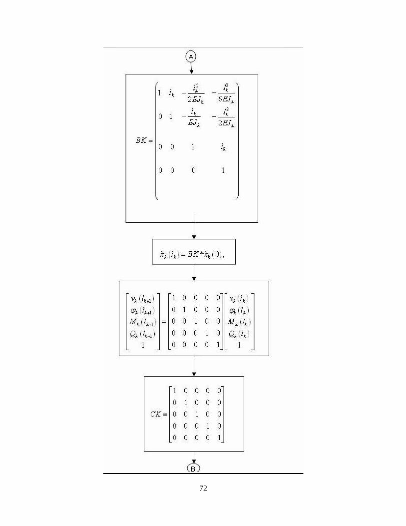
6.5.2 Flowchart
72
73

74
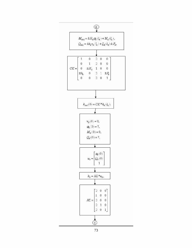
Fig 6.13. Flowchart for calculating the slope, displacement, moment and reaction of a beam
section with a various cross-sectional area and having vertical and angular stiffeners

75
6.5.3 Result
Fig.6.14. Problem Statement
SOLUTION-
M=56.2516 kN-m
P=20.615 kN
From Program
Fig.6.15. Solution obtained from Program

76
7
CONCLUSION

77
Transfer matrix is a powerful tool to solve for solving large type of problem using
computer programming. We have can taken advantage of this method of analysis to make
problem more simpler. The transfer-matrix method is used when the total system can be broken
into a sequence of subsystems that interact only with adjacent subsystems. To implement the
transfer matrix method, we need a relationship that gives the state of forces and displacements at
one end of the element in terms of force and displacement at the other end. Transfer matrix
method is an approach to matrix structural analysis that uses a mixed form of the element force-
displacement relationship and transfers the structural behavior parameters the joint forces and
displacement from one end of the structures of line element to other). An advantage of transfer
matrix method is that it produces a system of equations that are to be solved that are quite small
in comparison with those produced by the stiffness method. A disadvantage is the extensive
sequence of operations that are required on a small matrix.

78
REFERENCES
• By Rajasekaran S. and Sankarasubramanian G., Computational Structural Mechanics,
New Delhi, Prentice-Hall of India Private Limited, 2001.
• By Tesar Alexander and Fillo Ludovit, Transfer Matrix Method, Czechoslovakia, Kluwer
Academic Publisher, 1988.
• By Kanetkar Yashavant, Let us C, New Delhi, BPB Publication, 2005.
• By Pandit G.S. and Gupta S.P., Structural Analysis A Matrix Approach, New Delhi, Tata
McGraw-Hill Publishing Company Limited, 1981.
• By Kanetkar Yashavant, Pointers in C, New Delhi, BPB Publication, 2005.
• By Kanetkar Yashavant, Data Structure in C, New Delhi, BPB Publication, 2005.
• www.wikipedia.com
• www.howstuffworks.com