transfer payments and the macroeconomy: the effects of ...dromer/papers/romer and romer...

American Economic Journal: Macroeconomics 2016, 8(4): 1–42 http://dx.doi.org/10.1257/mac.20140348

1

Transfer Payments and the Macroeconomy: The Effects of Social Security Benefit Increases,

1952–1991†

By Christina D. Romer and David H. Romer*

This paper uses Social Security benefit increases from 1952 to 1991 to investigate the macroeconomic effects of changes in transfers. It finds a large, immediate, and significant positive response of con-sumption to permanent benefit increases. The response declines after about five months, and does not appear to spread to industrial pro-duction or employment. The effects of transfers are faster, but much less persistent and much smaller overall, than those of tax changes. Finally, monetary policy responds strongly to benefit increases but not to tax changes. This may account for the failure of the effects of transfers to persist or spread. (JEL E21, E62, E63, H31, H55)

Government transfer payments are the relative unknowns of fiscal policy. There have been many studies of the short-run macroeconomic effects of changes in

government purchases and taxes, but much less research has been done on the aggre-gate impacts of transfer payments. Yet such payments are substantial. In the United States today, for example, federal transfer payments account for about 15 percent of GDP and more than 40 percent of federal spending. This paper takes a step toward filling this gap in our knowledge by examining the macroeconomic impact of increases in Social Security benefits in the United States from 1952 to 1991.1

For much of the postwar period, increases in Social Security benefits occurred somewhat randomly. The generosity of the program was expanded in several steps during the 1950s and 1960s. Until 1974, cost-of-living increases were not auto-matic, but were legislated at irregular intervals. And from 1975 until the early 1990s, substantial variation in inflation and occasional bursts of retroactive payments resulting from idiosyncratic factors, as well as a legislated change in the timing of cost-of- living adjustments, led to irregular and variable benefit changes. This

1 Oh and Reis (2012) document the importance of changes in transfers in short-run movements in government expenditures, and describe some of the channels through which they could have aggregate effects.

* C. Romer: Department of Economics, University of California, Berkeley, Berkeley, CA 94720-3880 (e-mail: [email protected]); D. Romer: Department of Economics, University of California, Berkeley, Berkeley, CA 94720-3880 (e-mail: [email protected]). We are grateful to Martin Eichenbaum, Simon Gilchrist, Yuriy Gorodnichenko, John Leahy, Ricardo Reis, the referees, and seminar participants at Stanford University, the University of California, Berkeley, Northwestern University, the University of Michigan, the University of Chicago, Princeton University, and the National Bureau of Economic Research for helpful comments and suggestions, and to Dmitri Koustas, Paul Matsiras, and Walker Ray for research assistance.

† Go to http://dx.doi.org/10.1257/mac.20140348 to visit the article page for additional materials and author disclosure statement(s) or to comment in the online discussion forum.

mailto:[email protected]

mailto:[email protected]

2 AMErIcAn EconoMIc JournAL: MAcroEconoMIcS ocToBEr 2016

variation makes Social Security benefit increases a potentially fruitful window into the macroeconomic effects of transfers.

We use documents from the Social Security Administration, Congress, and the executive branch to identify the nature, motivation, timing, and size of benefit increases over these decades. This narrative analysis allows us to focus on increases that raised payments to existing beneficiaries, to exclude the few increases that were explicitly made for countercyclical purposes, and to separate permanent and tempo-rary changes.

We then estimate how aggregate consumer spending responds to these relatively exogenous increases in Social Security benefits. We find that permanent benefit increases have a roughly one-for-one impact on consumer spending in the month the larger checks arrive, and that this effect is highly statistically significant. The effect persists for roughly half a year and then appears to wane sharply—though the standard errors become large at longer horizons. Interestingly, we find that tempo-rary benefit increases (which mainly took the form of one-time retroactive payments in the period we consider) have a much smaller impact on consumption. Neither permanent nor temporary increases in benefits appear to affect broader measures of economic activity, such as industrial production or employment.

In some models of macroeconomic behavior, taxes and transfers have equal and opposite effects on household consumption and overall economic activity. To com-pare the effects of taxes and transfers, we expand our analysis to also include the rela-tively exogenous federal tax changes identified in Romer and Romer (2010). Like the permanent Social Security benefit increases, these tax changes were almost all legis-lated to be very long-lasting. We find large differences in the response of consump-tion to a permanent benefit increase and a tax cut. The effects of a benefit increase are faster, but much less persistent and substantially smaller overall. In both cases, the main component of consumption that responds is purchases of durable goods.

One possible explanation for the seemingly short-lived response of consump-tion to a permanent benefit increase, and the contrast with the impact of a tax cut, involves the response of monetary policy. We therefore examine both statistical and narrative evidence on the monetary policy reaction. We find that the federal funds rate rises in response to a benefit increase, and the effect is very fast, economically large, and highly statistically significant. Following an exogenous tax cut, in con-trast, the federal funds rate falls slightly over the first year. The records of Federal Reserve policy discussions reveal that policymakers were very aware of the benefit increases and often viewed them as a reason to tighten monetary policy. In contrast, monetary policymakers were much less consistent in advocating for counteracting the likely impacts of tax changes on aggregate demand.

The most important limitation of our study is simply that the amount of iden-tifying variation that we are able to exploit is only moderate. Increases in Social Security benefits are small relative to the large changes in government purchases associated with major wars, and they are noticeably smaller than the tax changes that are the focus of Romer and Romer (2010). Our detailed information about the monthly timing of benefit increases allows us to pin down their effects in the very near term relatively precisely. But once we consider horizons beyond a few months, the limited amount of variation often yields confidence intervals that are

VoL. 8 no. 4 3ROMER AND ROMER: TRANSFER PAYMENTS AND THE MACROECONOMY

wide enough to encompass a range of economically interesting hypotheses. Thus, this paper is only a first step in trying to understand the macroeconomic effects of government transfer payments.

Our paper builds on and speaks to a range of literatures. Many papers examine the response of individuals to particular changes in income. Most find that as long as the changes are not large, individuals respond to them when they occur, even if they could have known about them in advance or their impact on lifetime resources is small.2 Importantly, although this individual-level evidence is suggestive of a macroeconomic impact of changes in transfers, there could be offsetting forces at the aggregate level. For example, there could be Ricardian-equivalence effects: the adverse implications for lifetime wealth of the higher future taxes needed to finance an increase in transfers could exert a downward influence on all individuals’ consumption. Likewise, there could be offsetting effects on aggregate consump-tion through higher interest rates, reduced confidence about government policy, or increased uncertainty about policy. Thus, a finding that individuals who receive a payment raise their consumption relative to individuals who do not is insufficient to establish that changes in transfers have important macroeconomic effects. It is therefore important to look directly at aggregate evidence.

Like us, Wilcox (1989) looks at the response of aggregate consumption to Social Security benefit increases. Like much of the individual-level literature, however, his focus is on the permanent income hypothesis: since the benefit increases are announced in advance, the hypothesis implies that consumption should not respond to their implementation. He shows that over the period 1965–1985, the immediate impact of permanent benefit increases on real retail sales and personal consump-tion expenditures is positive and statistically significant. Because our interest is in the macroeconomic effects of changes in transfers more broadly, we use narrative sources to construct a longer sample of benefit increases, and to identify and omit the few that were made in response to short-run macroeconomic developments. In our empirical analysis, we focus on the magnitude of the effects of benefit increases rather than just whether they are nonzero, examine whether the impact persists and whether it spreads to broader indicators of economic activity, and compare the effects of permanent and temporary benefit changes. We go on to compare the effects of transfers and tax changes, and to investigate the response of monetary policy. While we replicate Wilcox’s finding of a strong immediate impact of permanent benefit increases on consumption, we find that the effects disappear relatively quickly and do not spread, and we provide evidence that counteracting monetary developments likely explain much of this behavior.

Our paper is clearly related to recent work on the macroeconomic effects of changes in fiscal policy. These papers use both time-series evidence and cross-state variation.3 While this literature has generally found a significant positive impact of

2 See, for example, Agarwal, Liu, and Souleles (2007); Sahm, Shapiro, and Slemrod (2012); and Parker et al. (2013).

3 Among the papers using time-series evidence are Blanchard and Perotti (2002), Hall (2009), Fisher and Peters (2010), Romer and Romer (2010), Barro and Redlick (2011), and Ramey (2011). Among the papers using cross-state variation are Shoag (2010), Chodorow-Reich et al. (2012), and Nakamura and Steinsson (2014). Pennings (2016) finds that in response to Social Security benefit increases over the period 1968–1974, labor income


fiscal expansion, the implied fiscal multipliers differ substantially in both size and timing. Our paper provides another estimate of the effect of fiscal policy, using a type of fiscal change whose timing is relatively exogenous and can be identified quite accurately.

Finally, much recent research has focused on the importance of monetary pol-icy for the effects of fiscal policy (for example, Leigh et al. 2010; Christiano, Eichenbaum, and Rebelo 2011; Woodford 2011; and Nakamura and Steinsson 2014). Our study provides both statistical and narrative evidence of a link between Social Security benefit increases and contractionary monetary policy, and of differ-ent monetary policy responses to changes in transfers and taxes.

Our analysis is organized as follows. Section I discusses our use of narrative sources to identify the nature, motivation, timing, size, and permanence of Social Security benefit increases. Section II examines the response of consumption and other aggregate indicators to relatively exogenous benefit increases. Section III compares the impact of benefit increases and tax changes. Section IV investigates the response of monetary policy to benefit increases and tax changes using both statistical evidence and evidence from the records of Federal Reserve policy discus-sions. Finally, Section V presents our conclusions and discusses the implications of our findings.

I. Identifying Social Security Benefit Increases

A central goal of the paper is to use Social Security benefit increases to examine how consumption and other macroeconomic variables respond to changes in trans-fer payments. Thus, a critical step is to identify a set of benefit increases that are useful for this purpose.

A. General considerations

There exist monthly data on aggregate Social Security payments in the National Income and Product Accounts (NIPA) starting in 1959, and administrative data on payments from the Social Security Administration going back further. However, not all increases in aggregate Social Security benefit payments are appropriate for esti-mating the near-term effects of changes in transfers. First, changes in benefit pay-ments reflect changes in both the number of beneficiaries and the size of benefits. But changes in payments resulting from changes in the number of beneficiaries are likely to be correlated with other factors affecting the economy, such as demographic changes raising the number of individuals over the retirement age or endogenous retirement decisions in response to the health of the economy. Likewise, changes in payments coming from legislated expansions in eligibility for Social Security may affect consumption and activity through very different channels than changes in payments to existing recipients. For this reason, we want to limit the analysis to benefit increases stemming from increased payments to existing beneficiaries.

rose more in states where Social Security benefits were larger relative to state income, suggesting an impact of the changes on local spending.


A second consideration is that, like changes in coverage, legislated changes in the path of future benefits or in the retirement age are likely to affect behavior through very different mechanisms than those for immediate benefit changes. We therefore also exclude such longer run changes from the analysis.

A third issue is that Social Security benefits were occasionally increased for explicitly countercyclical reasons. In such cases, one might not expect consumption to rise following the increases in benefits because other factors (that is, whatever was causing the economy to be weak) were operating in the opposite direction. For this reason, we need to identify the motivation for legislated benefit increases, and exclude any that were explicitly motivated by the state of the economy.

Finally, while most Social Security benefit changes have been intended as per-manent, some were explicitly temporary. For example, some permanent benefit increases were retroactive for several months. In these cases, in the month of the increase, beneficiaries received not only their higher regular monthly benefit, but also a one-time payment for the higher benefits in the preceding months. Many models of consumer behavior predict that permanent and temporary changes in income have very different impacts. For this reason, it is important to classify ben-efit increases into whether they were permanent or temporary, and to consider the two types of changes separately.

B. Methods used for 1952–1974

As just described, isolating Social Security benefit increases that are useful for estimating the macroeconomic effects of changes in transfers requires evidence about the nature and motivation for benefit changes. Thus, we need to bring in infor-mation beyond the standard data sources.

We begin our analysis of Social Security benefit increases in the early 1950s. This is late enough that the Social Security program was well established and operating at a substantial scale; at the same time, it is early enough that it captures the substantial changes in benefits in the 1950s and early 1960s. To identify useful observations on benefit increases for the first part of the sample, we focus on legislated changes. This focus automatically excludes any change in payments occurring through demo-graphic developments and endogenous retirement decisions.

We identify the universe of possible legislated changes using a Congressional Research Service survey (Kollmann and Solomon-Fears 2001). The descriptions in the survey allow us to identify the acts that may have affected the benefits of existing beneficiaries, and to exclude the acts that only affected coverage. We also use the descriptions to exclude several other types of actions: ones that only affected pay-ments to future beneficiaries, ones involving only small administrative changes, and ones that did not ultimately lead to the enactment of legislation.

We look at a range of narrative sources to identify important characteristics of each relevant legislated increase. The Social Security Bulletin typically has an arti-cle describing the specifics of the legislation and providing a detailed account of the Congressional debate. This article often provides the most comprehensive informa-tion about the nature, size, timing, and permanence of the increase (Social Security Bulletin, various issues). The reports of the House Ways and Means Committee and


the Senate Finance Committee on the bill typically contain information about the motivation for the action as well as its size, though the final legislation often differs at least slightly from the versions analyzed in these reports (US Congress, various years). The Economic report of the President often discusses both the motivations for the actions and their sizes (US Office of the President, various years). Finally, presidential speeches, particularly those made proposing the legislation or upon the signing of the final bill, are also useful sources (Woolley and Peters 1999).

We date the changes according to the month when Social Security checks reflected the benefit increase. Our sources do not provide enough information to generate a reliable series on the timing of the news surrounding the increases. But, as a step in that direction, we collect information on the date of passage for each benefit change. The narrative record also makes clear which benefit increases were one-time pay-ments and which were permanent.

We try to identify the aggregate increase in payments to current recipients (at an annual rate) in the first month the higher payments were received. As a practi-cal matter, this is typically derived from the cost estimates of the legislation in the first period mentioned (which is usually the first full year). We include increases in old-age, survivors, and disability benefits, since they are often combined in the dis-cussions in our sources. We also include increases in Supplemental Security Income (SSI) benefits, which provide additional support for low-income seniors and dis-abled individuals.

Finally, we gather information on the motivations for the increases. The vast majority were undertaken either to allow benefits to make up for inflation that had occurred over the previous several years, or for equity reasons. For example, the increase legislated in the Social Security Act Amendments of 1952 was intended to make up for the inflation that had occurred after the outbreak of the Korean War in 1950. The increase in the Tax Reform Act of 1969 was motivated by a desire both to counter the inflation of the previous few years and to ensure that the standard of living of the elderly rose along with that of the general population. A few benefit increases, however, were explicitly undertaken for countercyclical purposes. For example, the timing of the benefit increase contained in the Social Security Amendments of 1961 was explicitly tied to the need to raise demand to counteract economic weakness. As described above, because these changes are likely correlated with other factors affecting the economy in the short run, we exclude these anti-recessionary increases from our analysis of the macroeconomic effects of the benefit changes.

Online Appendix A provides a brief description of each legislated increase in benefits and the key information about it.

C. Methods used for 1975–1991

Starting in 1975, Social Security benefits were indexed to inflation. Because these cost-of-living increases raised existing benefits, rather than expanded coverage, they are potentially useful observations. Similarly, because these benefit increases were automatic, there is no issue of them being deliberately countercyclical. At the same time, because inflation responds to the state of the economy, benefit increases due


to indexation could potentially be correlated with other developments affecting con-sumption and economic activity. We address this issue in detail in Section II.

Two features of these automatic adjustments through the early 1990s allow them to provide useful variation. One is that the timing of the cost-of-living increases switched at one point: they occurred in July until 1982 and in January starting in 1984 (with no adjustment in 1983). The other is that there was substantial heteroge-neity in the size of the adjustments: they ranged from 1.3 percent in January 1987 to 14.3 percent in July 1980. After 1991, however, inflation was very low and the adjust-ments so regular that it seems unlikely that they greatly affected behavior. Moreover, their regularity means that any impact on macroeconomic outcomes would probably have been obscured by the seasonal adjustment of the data.4 For this reason, we only construct a series on these automatic benefit increases through December 1991.

Legislation played a very small role in benefit changes in the 1975–1991 period. The Congressional Research Service survey described above shows that the vast majority of legislated changes in this period affected coverage or future payments, not the benefits of existing recipients. The one notable exception was the Social Security Amendments of 1983, which was the source of the change in the timing of the automatic cost-of-living adjustments and also raised Supplemental Security Income payments.

There were also some one-time payments in this period whose timing was effec-tively random. In particular, there were one-time retroactive payments at various dates based on legal decisions, revisions to case review procedures, and, in one case, the purchase of new computers that sped the processing of appeals. We iden-tify these one-time payments by conducting Google news searches using the terms “Social Security” and “personal income,” and “Social Security” and “retroactive.”

Because the benefit increases in this period were not legislated, for the most part their sizes are not reported in our sources. Thus, our methods for estimating sizes differ from those we use for the earlier period. For the cost-of-living adjustments, we multiply total Social Security payments (as reported in the NIPA data) in the month before the increase by the official percentage adjustment.5 This procedure holds enrollment fixed, and so shows just the increase in payments coming from the increase in average payments per beneficiary.

In the case of the one-time payments, occasionally the news stories discuss their size, but often they do not. To estimate the size of a payment, we therefore take the increase in the NIPA Social Security series in the month for which our news stories identify a payment. Since the usual month-to-month changes in this series are small, most of the changes in the months of substantial one-time payments are likely the result of the payments. Consistent with this interpretation, the estimates based on this approach correlate closely with the figures in the news articles in the few cases where the articles report the sizes of the one-time payments.

4 Because the Bureau of Economic Analysis (BEA) obtains many of the component consumption series only in seasonally adjusted form, it does not construct seasonally unadjusted consumption data. Thus, it is not possible to examine the impact of the regular annual adjustments on seasonally unadjusted consumption.

5 The monthly NIPA Social Security data are from the BEA, NIPA, table 2.6, series for government social ben-efits to persons—Social Security, downloaded January 23, 2014.


We classify the automatic cost-of-living increases as permanent and the various one-time payments as temporary. Online Appendix A provides additional details about the cost-of-living increases and lists the sources of the articles about the one-time payments.

D. new Series of Social Security Benefit Increases

Table 1 presents the data for the full 1952–1991 period. They are expressed as the dollar increase as a percent of aggregate personal income.6 Permanent and tempo-rary increases are reported separately. Figure 1 shows the two series.

The figure shows several characteristics of the new series. One is that the timing of benefit increases was highly uneven, particularly before 1975. This adds cre-dence to the notion that there is substantial usable variation to exploit. At the same time, the size of the permanent benefit increases varied within a somewhat narrow range. The largest permanent increase was less than 1 percent of aggregate personal income. In contrast, some temporary benefit increases were quite large. The three

6 The monthly data on personal income are from the BEA, NIPA, table 2.6, http://www.bea.gov/iTable/index_nipa.cfm, downloaded January 23, 2014. For the years before 1959, we use the quarterly personal income figures (from table 2.1, downloaded January 23, 2014) for each month of the quarter.

Table 1—New Series of Permanent and Temporary Social Security Benefit Increases, 1952–1991( percent of personal income)

1952–1974 1975–1991

Date Permanent Temporary Date Permanent Temporary

October 1952 0.23 July 1975 0.37October 1954 0.21 July 1976 0.31December 1956 0.14 July 1977 0.29August 1957 0.07 July 1978 0.31October 1958 0.05 July 1979 0.46February 1959 0.18 July 1980 0.68December 1960 0.05 July 1981 0.56January 1961 0.06 July 1982 0.39September 1965 0.39 1.81 August 1983 0.03January 1966 0.03 November 1983 0.17November 1966 0.02 December 1983 0.21March 1968 0.49 January 1984 0.19April 1970 0.48 0.96 December 1984 0.25June 1971 0.37 1.46 January 1985 0.19October 1972 0.75 July 1985 0.16February 1973 0.21 January 1986 0.16February 1974 0.14 July 1986 0.17April 1974 0.33 January 1987 0.07July 1974 0.19 May 1987 0.16August 1974 0.01 January 1988 0.21

March 1988 0.12January 1989 0.19March 1989 0.14November 1989 0.08January 1990 0.22January 1991 0.27

notes: See online Appendix A for a detailed description of each benefit increase. The text describes the source of the personal income data used to scale the series.

http://www.bea.gov/iTable/index_nipa.cfm

http://www.bea.gov/iTable/index_nipa.cfm


largest one-time payments (in 1965, 1970, and 1971) were each about 1 to 2 percent of annual personal income. And most of the later one-time payments, though not as large relative to aggregate personal income, were large for those receiving them. Our news stories provide figures for the average payment per recipient for three of these one-time payments: those in November–December 1983, December 1984, and July 1986. In 2014 dollars, these payments averaged $2,335 per recipient in 1983, $1,075 in 1984, and $572 in 1986.

E. Persistence of Permanent Benefit Increases

Many of the benefit increases we classify as permanent were intended to make up for past inflation. But, since inflation itself was serially correlated, there may have been a tendency for even permanent benefit increases to be eroded by future inflation, and so for their effects on income to be only moderately persistent. To shed light on this issue, we look at the relationship between the NIPA series on Social Security benefits as a share of personal income (which is available starting in 1959) and our series on permanent and temporary benefit increases.

In particular, we estimate the following regression:

(1) Δ B t = a + ∑ i=0

n

b i PErM S S t−i PErM + ∑ i=0

n

b i TEMP S S t−i TEMP + e t ,

where ΔB is the change in the ratio of the monthly NIPA measure of Social Security benefits to personal income, and S S PErM and S S TEMP are our new series on permanent and temporary increases in Social Security benefits, both measured as a fraction of personal income. n is the number of lags. We estimate the regression

0.0

0.2

0.4

0.6

0.8

1.0

1.2

1.4

1.6

1.8

2.0

1952

:1

1954

:1

1956

:1

1958

:1

1960

:1

1962

:1

1964

:1

1966

:1

1968

:1

1970

:1

1972

:1

1974

:1

1976

:1

1978

:1

1980

:1

1982

:1

1984

:1

1986

:1

1988

:1

1990

:1

Per

cent

of p

erso

nal i

ncom

e Temporary

Permanent

Figure 1. New Series of Permanent and Temporary Social Security Benefit Increases ( percent of personal income)

note: See text and online Appendix A for details of the new series.


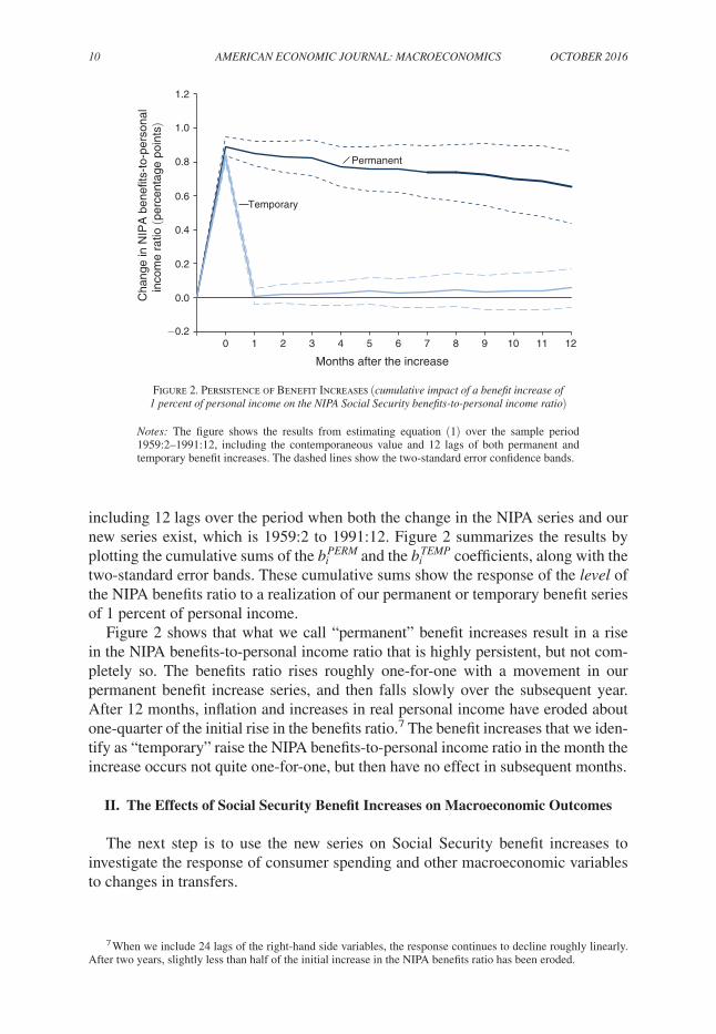
including 12 lags over the period when both the change in the NIPA series and our new series exist, which is 1959:2 to 1991:12. Figure 2 summarizes the results by plotting the cumulative sums of the b i PErM and the b i TEMP coefficients, along with the two-standard error bands. These cumulative sums show the response of the level of the NIPA benefits ratio to a realization of our permanent or temporary benefit series of 1 percent of personal income.

Figure 2 shows that what we call “permanent” benefit increases result in a rise in the NIPA benefits-to-personal income ratio that is highly persistent, but not com-pletely so. The benefits ratio rises roughly one-for-one with a movement in our permanent benefit increase series, and then falls slowly over the subsequent year. After 12 months, inflation and increases in real personal income have eroded about one-quarter of the initial rise in the benefits ratio.7 The benefit increases that we iden-tify as “temporary” raise the NIPA benefits-to-personal income ratio in the month the increase occurs not quite one-for-one, but then have no effect in subsequent months.

II. The Effects of Social Security Benefit Increases on Macroeconomic Outcomes

The next step is to use the new series on Social Security benefit increases to investigate the response of consumer spending and other macroeconomic variables to changes in transfers.

7 When we include 24 lags of the right-hand side variables, the response continues to decline roughly linearly. After two years, slightly less than half of the initial increase in the NIPA benefits ratio has been eroded.

−0.2

0.0

0.2

0.4

0.6

0.8

1.0

1.2

0 1 2 3 4 5 6 7 8 9 10 11 12

Cha

nge

in N

IPA

ben

efits

-to-

pers

onal

inco

me

ratio

(per

cent

age

poin

ts)

Months after the increase

Temporary

Permanent

Figure 2. Persistence of Benefit Increases (cumulative impact of a benefit increase of 1 percent of personal income on the nIPA Social Security benefits-to-personal income ratio)

notes: The figure shows the results from estimating equation (1) over the sample period 1959:2–1991:12, including the contemporaneous value and 12 lags of both permanent and temporary benefit increases. The dashed lines show the two-standard error confidence bands.


A. outcome Variables and Sample Periods

The main outcome variable we consider is real personal consumption expendi-tures.8 There are two main advantages of focusing on consumption. First, because increases in Social Security benefits affect households’ disposable income directly, any macroeconomic effects might occur more quickly and sharply in consumption than in other aggregate variables. Second, consumption data are available monthly, which allows us to use information about the exact timing of benefit increases more effectively than we could with lower frequency data.

One drawback of the monthly consumption series is that it is not available before 1959. However, both quarterly data on real consumption and monthly data on real retail sales (which generally move closely with consumption) are available for the earlier period. We therefore construct monthly consumption data for the period before 1959 using a Chow-Lin procedure.9

We consider three other aggregate outcome series: real retail sales, industrial pro-duction, and employment. All three are available monthly beginning before 1950.10 Retail sales are more volatile than consumption but capture a similar aspect of the economy. In contrast, industrial production and employment are broader indicators of economic activity, and so may respond differently to increases in Social Security benefits.

Our baseline sample period is 1952–1991. We consider two variants of the base-line sample. The first starts in 1959, and so excludes the period for which we have only estimated monthly consumption data. The second ends in 1974, and so excludes the period when benefit increases were largely the result of automatic cost-of-living adjustments.

B. Specification and Identification Issues

Baseline Specification.—Our goal is to estimate the effects of permanent and temporary Social Security benefit increases on consumption and other aggregate

8 The data are from the BEA, NIPA, table 2.8.3, series for personal consumption expenditures, downloaded January 23, 2014.

9 The data on retail sales, adjusted for seasonal variation, for 1947:1–1958:12 are from the US Department of Commerce, Business Statistics (1979, 216). We convert it to a real series by dividing by the seasonally adjusted consumer price index for all urban consumers: all items less shelter, Bureau of Labor Statistics (BLS), series CUSR0000SA0L2, downloaded from Federal Reserve Economic Data (FRED) http://research.stlouisfed.org/fred2/, January 23, 2014. The quarterly real consumption data are from the BEA, NIPA, table 2.3.3, series for personal consumption expenditures, downloaded January 23, 2014. To create an estimate of monthly consumption, we use the Chow-Lin algorithm in RATS, which employs the variant of the Chow-Lin procedure proposed by Fernández (1981). We estimate the algorithm over the period 1947–1958. The results are similar for this decade when we run the Chow-Lin procedure over the full sample 1947–1991.

10 The real retail sales series for 1947–1991 is constructed by taking nominal, seasonally adjusted data for 1967:1–1991:12 from the US Department of Commerce, Business Statistics (1991, A-56 and 37); for 1961:1–1967:1 from Business Statistics (1984, 177); and for 1947:1–1961:1 from Business Statistics (1979, 216). The series, which do not line up exactly because of data revisions, are combined using ratio splices—starting with the most recent series and working backwards. The data are converted to real values by dividing by the consumer price index for all urban consumers: all items less shelter. The industrial production series is the total index, sea-sonally adjusted, Board of Governors of the Federal Reserve System, series INDPRO, downloaded from FRED, January 24, 2014. The employment series is total nonfarm employees, seasonally adjusted, BLS, series PAYEMS, downloaded from FRED, January 24, 2014.

http://research.stlouisfed.org/fred2/

http://research.stlouisfed.org/fred2/


outcome measures. As described in Section I, the benefit increases we identify were largely a response to past inflation or to equity and fairness considerations. Thus, there is no reason to expect them to be systematically correlated with contempora-neous macroeconomic conditions or with other short-run influences on macroeco-nomic outcomes. In addition, as discussed above, a range of evidence suggests that households respond to modest changes in income when the changes occur rather than when they learn that the changes will happen.

This discussion suggests that a natural starting point for estimating the impact of benefit increases on macroeconomic outcomes is very simple. We begin by con-sidering regressions of an outcome variable on the contemporaneous and lagged values of our measures of increases in Social Security benefits, with no controls, and with the benefit increases dated according to when recipients first received checks reflecting the higher benefits. Since permanent and temporary benefit increases have been quite different in character and might have different effects, we enter them separately. That is, the baseline specification takes the form

(2) Δ ln Y t = a + ∑ i=0

n


n


where Δ ln Y is the change in the logarithm of an outcome variable—primarily real personal consumption expenditures—and n is the number of lags.

Of course, the conditions needed for this specification to be appropriate may not hold exactly. Three concerns appear particularly important.

news.—It is possible that recipients respond not only when they receive higher benefits, but also when there is news of benefit increases. To the extent this is the case, equation (2) omits a determinant of consumption or other macroeconomic outcomes that may be correlated with our benefit series.

We address this concern in two ways. First, we experiment with including sev-eral leads of the benefit increases in (2). This allows for the possibility that house-holds change their behavior in anticipation of the increases. Second, in addition to including the contemporaneous and lagged values of benefit increases dated when they showed up in recipients’ checks, we include the contemporaneous and lagged values of the increases dated when they were passed. If consumption responds to news rather than to changes in current income, its movements will be more closely related to when the increases were passed than to when recipients first received the higher benefits.

Macroeconomic Endogeneity.—The second and largest set of concerns revolves around the role of macroeconomic developments in leading to the benefit increases. As discussed above, a substantial fraction of the increases were motivated by a desire to make up for past inflation. Thus, it is natural to be concerned about the possibility that consumption movements or other macroeconomic outcomes follow-ing these benefit increases were in part responses not to the benefit increases, but to factors that caused the inflation that prompted the increases. For example, a pro-longed economic boom could both cause inflation that led to a benefit increase and


directly generate higher consumption. Similarly, a period of sustained growth could make it more likely for policymakers to increase benefits on grounds of fairness, and some of the behavior of macroeconomic variables following these increases could be responses to the factors that caused the high growth rather than to the benefit increases.

Although these possibilities could be relevant to studies of some relationships, they are unlikely to be problematic for our analysis. Before 1974, the benefit increases were ad hoc, infrequent, and irregularly spaced. Even after the adoption of indexing, benefit adjustments still occurred at discrete intervals. As a result, the relationship between the benefit increases and macroeconomic developments is weak. For exam-ple, a regression of our series for permanent benefit increases on a constant and 12 lags of inflation, estimated over our full sample period 1952:1–1991:12, yields an

_ r 2 of just 0.01.11 Similarly, a regression of the permanent benefit increases on

a constant and 12 lags of consumption growth has an _

r 2 of −0.0003. Thus, even if various factors were affecting benefit increases through effects on inflation or growth, their correlation with the actual benefit increases is likely to be small.

Nonetheless, we take several steps to address the possibility that the benefit increases were to some extent endogenous responses to macroeconomic develop-ments and that this could be affecting the results. First, we consider the effects of stopping the sample in 1974, and so leaving out the period when benefit increases were most mechanically linked to inflation. Second, we experiment with adding some drivers of inflation as control variables in (2). One is the change in oil prices. A rise in oil prices could both directly reduce real consumption spending and raise inflation (and hence lead to benefit increases), and so bias our estimates down. Another is a measure of monetary policy shocks, which are a potential source of movements in economic activity and inflation.

Including the controls serves another purpose in addition to dealing with possible omitted variable bias from the responsiveness of benefits to inflation: it addresses potential sources of accidental correlation between the benefit increases and other influences on macroeconomic variables. That is, perhaps benefit increases do not actually respond to oil price movements or monetary policy shocks, but there just happen to be strong movements in those variables around the times of the benefit increases.

Finally, and most importantly, we embed the benefit increases in a vector autore-gression (VAR) framework. The VARs account for possible correlation between the benefit increases and past macroeconomic developments, and they account for the normal dynamics of the macroeconomy. Our baseline VAR includes the two ben-efit series (permanent and temporary) and the focal outcome variable (consump-tion). We also consider specifications that include the price level to account for the potential role of inflation in driving benefit increases. Because we want to find the effects of both permanent and temporary benefit increases, which often occur together, our identifying assumption throughout is that permanent and temporary

11 The specific inflation series we use is the change in the logarithm of the seasonally adjusted consumer price index for all urban consumers: all items, BLS, series CPIAUCSL, downloaded from FRED, January 23, 2014.


benefit increases do not cause one another within the month, and that both can affect but are not affected by the other variables in the system within the month.12

other Fiscal Actions.—The final set of concerns involves the possibility that increases in Social Security benefits could be correlated with other fiscal actions. There are two main issues. First, perhaps benefit increases were legislated as parts of expansionary fiscal packages more broadly. Second, because the Social Security program is explicitly self-financed, legislation increasing benefits has often included provisions raising payroll taxes.

The history of the Social Security program suggests that these possibilities are not major causes for concern. Our narrative analysis of the history of the benefit increases shows that most benefit increases were self-contained actions, not part of a broader program of fiscal expansion. This pattern is extremely clear for the second part of the sample, when benefit increases were almost entirely the result of automatic cost-of-living adjustments, and for the 1950s, when Social Security leg-islation was considered essentially in isolation. But it also appears to be an accurate description of most of the increases in the 1960s and early 1970s. In addition, we explicitly exclude the increases that were part of a countercyclical stimulus package, such as the one-time payments to seniors in the Tax Reduction Act of 1975.

In previous work (Romer and Romer 2010), we identified increases in Social Security taxes intended to pay for benefit increases from the same types of nar-rative sources described above. Many of these increases occurred years after the benefit increases, and even the increases that happened relatively quickly typically followed the benefit increases by at least a few months. For example, the Social Security Amendments of 1954, which raised benefits starting in October of that year, legislated a rise in the Social Security tax base in 1955 and increases in the Social Security tax rate in 1970 and 1975. Thus, the tax changes are unlikely to pose a major problem for our analysis, especially when we consider the very short-run effects of benefit increases.

To explicitly address the possibility of confounding effects from other fiscal actions, in Section III we consider specifications that include a measure of tax changes as a control variable. This approach also allows us to compare the effects of benefit increases and tax changes.

Controlling for other changes on the spending side of fiscal policy is harder. Monthly data on government purchases are not available, so there is no obvious control variable to include. However, a first look at the data suggests little reason for concern. In quarterly data, the contemporaneous correlation of our series for permanent Social Security benefit increases with the growth rate of real federal gov-ernment purchases is −0.04; its correlation with the growth rate of all of real federal government spending excluding Social Security benefits is −0.05; and its correlation

12 Thus, relative to VARs identified purely by an ordering assumption, we impose one additional restriction (by assuming that neither permanent nor temporary increases cause the other contemporaneously, rather than allow-ing one to affect the other), and relax one restriction (by allowing the shocks to permanent and temporary benefit increases to be correlated contemporaneously). Thus, like VARs identified by an ordering assumption, our VARs are just identified.


with the measure of shocks to government spending developed by Ramey (2011) is −0.01.13

C. results for the Baseline Specification

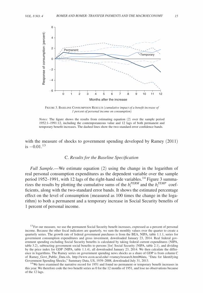
Full Sample.—We estimate equation (2) using the change in the logarithm of real personal consumption expenditures as the dependent variable over the sample period 1952–1991, with 12 lags of the right-hand side variables.14 Figure 3 summa-rizes the results by plotting the cumulative sums of the b i PErM and the b i TEMP coef-ficients, along with the two-standard error bands. It shows the estimated percentage effect on the level of consumption (measured as 100 times the change in the loga-rithm) to both a permanent and a temporary increase in Social Security benefits of 1 percent of personal income.

13 For our measure, we use the permanent Social Security benefit increases, expressed as a percent of personal income. Because the other fiscal indicators are quarterly, we sum the monthly values over the quarter to create a quarterly series. The growth rate of federal government purchases is from the BEA, NIPA, table 1.1.1, series for government consumption expenditures and gross investment, downloaded January 23, 2014. Real federal gov-ernment spending excluding Social Security benefits is calculated by taking federal current expenditures (NIPA, table 3.2), subtracting government social benefits to persons [for] Social Security (NIPA, table 2.1), and dividing by the price index for GDP (NIPA, table 1.1.4), all downloaded January 23, 2014. We then calculate the differ-ence in logarithms. The Ramey series on government spending news shocks as a share of GDP is from column C of Ramey_Govt_Public_Data.xls, http://www.econ.ucsd.edu/~vramey/research.html#data, “Data for Identifying Government Spending Shocks,” Summary Data, US, 1939–2008, downloaded July 31, 2013.

14 We have examined the narrative record for 1951 and found no permanent or temporary benefit increases in this year. We therefore code the two benefit series as 0 for the 12 months of 1951, and lose no observations because of the 12 lags.

−6

−4

−2

0

2

4

6

0 1 2 3 4 5 6 7 8 9 10 11 12

Res

pons

e of

con

sum

ptio

n (p

erce

nt)


Temporary

Permanent

Figure 3. Baseline Consumption Results (cumulative impact of a benefit increase of 1 percent of personal income on consumption)

notes: The figure shows the results from estimating equation (2) over the sample period 1952:1–1991:12, including the contemporaneous value and 12 lags of both permanent and temporary benefit increases. The dashed lines show the two-standard error confidence bands.

http://www.econ.ucsd.edu/~vramey/research.html#data


The most striking result is the large, immediate response of consumption to a permanent increase in benefits. The point estimates suggest that a benefit increase of 1 percent of personal income raises aggregate consumption by 1.2 percent in the month the larger checks arrive, and that the effect persists for the next 5 months. The null hypothesis of no effect in the month of the increase is rejected with a t -statistic of 2.8. As detailed below, this result is very robust.

The standard errors rise as the horizon lengthens. As a result, five months after the benefit increase, the point estimate remains large (1.0) but is no longer statistically significant ( t = 0.9). Thereafter, the estimated effect declines. However, the esti-mates are sufficiently imprecise that it is not possible to reject either the hypothesis that the effect remains one-for-one or the hypothesis that it returns to zero.

The figure shows that the response to a temporary benefit increase of 1 percent of personal income appears considerably weaker. The estimated impact in the month of the increase is only 0.1 percent ( t = 0.5). The estimates remain small for several months after the temporary payment. Thereafter they rise considerably, but the stan-dard errors are sufficiently large that the possibility that this pattern is just statistical noise cannot be rejected.15

An obvious question is why the effects of permanent and temporary benefit increases appear to be so different. One possibility involves their sizes. A com-mon finding in previous work on consumption is that households tend to behave as rule-of-thumb or Keynesian consumers in response to small changes in income, but to follow the predictions of the permanent income hypothesis more closely for large changes (for example, Hsieh 2003). In our case, the permanent benefit increases we consider are generally small, while the increases that provide the bulk of the iden-tification for temporary changes are large. The biggest permanent benefit increase in our sample is a 20 percent rise in individuals’ benefits in October 1972, and only a few of the permanent increases exceed 10 percent. In contrast, the retroactive across-the-board increases in September 1965, April 1970, and June 1971 were all 30 percent or more of individuals’ normal monthly benefits. And all three payments were coupled with increases in permanent benefits, so that the total Social Security payments beneficiaries received in the month exceeded their previous monthly benefits by 45 percent or more. In addition, as described in Section I, the various one-time payments in the 1980s were often substantial for those who received them. Thus, our finding that the temporary benefit increases in our sample period for the most part did not lead to large immediate increases in consumption is consistent with previous evidence about consumer behavior.

Alternative Sample Periods.—The results of the baseline specification are rel-atively robust to the sample period. To keep things manageable, our discussion

15 Two considerations suggest that the large point estimates for the effects of temporary payments at longer horizons likely reflect sampling error rather than true effects of the payments. First, it is hard to think of a plausible mechanism that would cause households to raise their spending greatly 6 or 12 months after receiving a one-time payment. Second, closer examination of the data shows that the substantial estimated response at moderate horizons is largely the result of a few observations. For example, there was a sharp rise in consumption in early 1972, which followed a large retroactive increase in Social Security benefits in June 1971. Conventional accounts of this period attribute the rise in consumption to a cut in the excise tax on autos and abundant credit, not to the earlier one-time benefits payment (see, for example, Economic report of the President, 1973, 23).


of robustness and of the results of the various ways of dealing with the concerns about identification focuses on the effects of a permanent benefit increase. Online Appendix B presents figures corresponding to the various robustness checks that we describe in the text; these figures are denoted in parentheses with a “B” pre-fix. Restricting the sample to the period when official monthly consumption data exist (that is, starting in 1959) reduces the estimated effects of a permanent ben-efit increase on consumption slightly (online Appendix Figure B1a). Using the pre-1974 sample (before indexation), on the other hand, raises the estimated effects of a permanent benefit increase noticeably (online Appendix Figure B1b). In both samples, the initial impact on consumption remains highly statistically significant.

In contrast, when we limit the sample to the period after the adoption of index-ation (1975–1991), there is too little identifying variation to be informative (online Appendix Figure B1c). The point estimates suggest little effect of permanent benefit increases at short horizons and substantial negative effects at longer ones. At all horizons, however, the two-standard error confidence interval includes not just zero, but effects well over one.16

D. Addressing the Identification Issues

news.—As described above, we address the possibility that consumers respond before the benefit increases take effect in two ways. The first is by adding leads of the benefit increases to (2), and so allowing for the possibility that households change their behavior in anticipation of the increases. Specifically, since there is typically a lag of about two to four months from the passage of legislation to the actual increases in benefits, we experiment with including three leads of the benefit increases. When we do this, the coefficients on the leads are never close to statis-tically significant, and two of the three are negative rather than positive (online Appendix Figures B2a and B2b).

The second approach is to consider not only the benefit increases dated when the larger checks arrived, but also when they were passed.17 Since news about automatic cost-of-living adjustments inherently comes out gradually as inflation reports accu-mulate, for this robustness check we restrict our attention to the period when benefit increases were legislated directly. Thus, our sample period is 1952–1974, and we include the contemporaneous value and 12 lags of both series. Figure 4 shows the results. The estimated response to the passage of benefit increases is irregularly signed and always far from statistically significant. The estimated response to the arrival of larger benefit checks, in contrast, is large and positive; indeed, it is greater than in the baseline specification. The responses in the month of an increase and in the subsequent month are significantly different from zero. Thereafter, the standard

16 Wilcox (1989) also finds that the impact of benefit changes in the second half of his sample (1975–1985) is smaller and much less precisely estimated than in the first half of his sample (1965–1974).

17 In assigning benefit increases to the month of passage, we follow the convention that if passage occurred before the middle of the month, we assign it to that month; if passage occurred after the middle of the month, we assign it to the next month.


errors are quite large, which is unsurprising given the shorter sample and the close proximity of the passage of legislation and the receipt of higher benefit checks.

Macroeconomic Endogeneity.—The second set of identification issues revolves around the potential macroeconomic endogeneity of the benefit increases. We first deal with these issues narrowly. For example, as noted above, ending the sample in 1974, and so excluding the period after the start of indexation, increases the esti-mated effects somewhat. This is contrary to what one would expect if endogeneity of benefit increases was greater when the increases were mechanically linked to past inflation, and consumption, inflation, and benefit increases were being driven by common expansionary factors.

Controlling for the contemporaneous value and 12 lags of the change in the logarithm of the price of oil leads to a moderately higher estimated impact of a permanent benefit increase on consumption (online Appendix Figure B3a).18 The estimated contemporaneous impact rises from 1.23 percent ( t = 2.85) to 1.40 per-cent ( t = 3.20). This pattern could result if oil prices both contribute to higher ben-efit increases and directly reduce consumption, so that there is some downward bias in the estimated response of consumption when oil prices are not included.

We do not want to control for all movements in monetary policy, since the response of monetary policy to benefit increases may affect how the increases impact

18 The specific series for oil prices we use is the spot oil price: West Texas intermediate, Dow Jones & Company, downloaded from FRED, November 25, 2014.

−15

−10

−5

0

5

10

15

0 1 2 3 4 5 6 7 8 9 10 11 12

Res

pons

e of

con

sum

ptio

n (p

erce

nt)


Permanent, dated when legislation was passed

Permanent, dated when checks arrived

Figure 4. Consumption Results Including Both News and Receipt of Benefit Increases (cumulative impact of a permanent benefit increase of 1 percent of personal income,

dated both when larger checks arrived and when legislation was passed, on consumption)

notes: The figure shows the results from estimating equation (2) over the sample period 1952:1–1974:12, including the contemporaneous value and 12 lags of both permanent benefit increases dated when the larger checks arrived and permanent benefit increases dated when the legislation was passed (and excluding temporary benefit increases). The dashed lines show the two-standard error confidence bands.


the economy (an issue we investigate in depth in Section IV). As discussed above, however, it is reasonable to control for monetary policy shocks, since they could affect inflation (and hence benefit increases) and directly affect economic activity. We therefore control for the contemporaneous value and either 12 or 24 lags of the dummy variable for contractionary monetary policy shocks constructed by Romer and Romer (1989, 1994). Including this variable strengthens the findings slightly (online Appendix Figures B3b and B3c).

To address the issue of possible macroeconomic endogeneity more broadly, we embed the benefit increases in a VAR. Figure 5 displays the results of estimating the VAR that includes permanent and temporary benefit increases (both measured as a fraction of personal income) and the logarithm of real personal consumption expenditures, with 12 lags of each variable. Specifically, the figure shows the per-centage effect on the level of consumption of both a permanent and a temporary benefit increase of 1 percent of personal income, together with the two-standard error bands.19 The results are very similar to those of the baseline specification. The impact of a permanent benefit increase is 1.2 percent ( t = 2.9) contemporaneously and 1.1 percent ( t = 1.3) after 5 months. The estimated impact of a temporary ben-efit increase is very small at short horizons, and imprecisely estimated throughout.

Figure 6 shows the effects of adding the logarithm of the seasonally adjusted overall consumer price index to the VAR. The results are broadly similar to the

19 The standard errors are computed by taking 100,000 draws of the coefficient vector from a multivariate nor-mal distribution with mean and variance-covariance matrix equal to the point estimates and variance-covariance matrix of the regression coefficients.

Figure 5. Consumption Results from a Three-Variable VAR (cumulative impact of a benefit increase of 1 percent of personal income on consumption)

notes: The figure shows the results from estimating a vector autoregression including three variables (permanent benefit increases, temporary benefit increases, and the logarithm of per-sonal consumption expenditures) over the sample period 1952:1–1991:12. The dashed lines show the two-standard error confidence bands.

−6

−4

−2

0

2

4

6

0 1 2 3 4 5 6 7 8 9 10 11 12

Res

pons

e of

con

sum

ptio

n (p

erce

nt)


Temporary

Permanent


baseline case. The main difference is that the estimated response to a permanent benefit increase is noticeably larger than before. This is the opposite of what one would expect if the estimated consumption response in the baseline specification were a response to a boom leading to inflation and hence to the benefit increases, rather than a true effect of the benefit increases. The impact is now 1.4 percent ( t = 3.4) contemporaneously, remains above one and statistically significant through month 5, and is positive at almost all horizons. The estimated effects of temporary benefit increases fall slightly relative to the baseline specification, and are now even further from statistical significance.20

The overall message of our various efforts to deal with the possibility of omitted variables affecting both the benefit increases and consumption is that we find no evidence that this concern is driving our results. Indeed, if anything, the estimated effects become slightly stronger when we address this issue.

other Fiscal Actions.—The final set of identification issues involves fiscal policy. We address these in the next section, where we explicitly compare the effects of Social Security benefit increases and tax changes.

20 We also consider the effects of using the Jordà local projection approach (Jordà 2005) rather than VARs. Moving from VARs to the local projection approach has almost no impact on the estimates (online Appendix Figures B4a and B4b).

−6

−4

−2

0

2

4

6

0 1 2 3 4 5 6 7 8 9 10 11 12

Res

pons

e of

con

sum

ptio

n (p

erce

nt)


TemporaryPermanent

Figure 6. Consumption Results from a Four-Variable VAR (cumulative impact of a benefit increase of 1 percent of personal income on consumption)

notes: The figure shows the results from estimating a vector autoregression including four variables (permanent benefit increases, temporary benefit increases, the logarithm of prices, and the logarithm of personal consumption expenditures) over the sample period 1952:1–1991:12. The dashed lines show the two-standard error confidence bands.


E. other outcome Variables

We now turn to the effects of Social Security benefit increases on three other monthly measures of macroeconomic outcomes: real retail sales, industrial produc-tion, and employment. We estimate equation (2), replacing consumption with these alternatives. Table 2 shows the cumulative response of each variable to a permanent benefit increase of 1 percent of personal income. The table also repeats the results for personal consumption expenditures (PCE) for comparison.

For retail sales, the point estimates suggest a somewhat larger impact of benefit increases than they do for consumption. For example, the estimated effect of a per-manent benefit increase of 1 percent of personal income is a rise in retail sales of 1.7 percent in the month it occurs, and a peak increase of 2.1 percent after 4 months. The standard errors, however, are also larger. The t -statistic on the contemporaneous effect is 1.7, and that on the maximum effect is 1.0. All of this is consistent with the fact that retail sales are more cyclically sensitive and more volatile than overall consumption.

The point estimates also suggest a nontrivial impact on industrial production. The estimated peak effect is 0.7 percent 3 months after a permanent benefit increase. The dominant feature of the estimates, however, is their imprecision. The t -statistics for the estimated positive effects never exceed 1, and the estimated impact turns sharply (but insignificantly) negative after 6 months.

Finally, there is no evidence of an employment response. The point estimates differ trivially from zero for five months before turning moderately negative. The hypothesis that the effect is zero cannot be rejected at any horizon.

Table 2—Baseline Results for Other Macroeconomic Outcome Variables (cumulative impact of a permanent benefit increase of 1 percent of personal income,

in percent)

Real PCE

Real retail sales

Industrial production Employment

Month Impact SE Impact SE Impact SE Impact SE

0 1.23 0.43 1.67 0.95 0.37 0.73 0.00 0.211 1.04 0.58 2.07 1.28 0.31 0.98 0.06 0.282 0.94 0.71 1.64 1.57 0.66 1.20 0.01 0.343 1.03 0.83 1.97 1.83 0.67 1.39 0.00 0.404 1.01 0.93 2.13 2.05 0.39 1.57 −0.01 0.455 0.96 1.03 1.46 2.27 −0.28 1.73 −0.12 0.496 0.36 1.13 0.09 2.49 −1.81 1.90 −0.37 0.547 0.02 1.23 −0.59 2.71 −2.05 2.06 −0.55 0.598 −0.32 1.33 −0.53 2.93 −2.52 2.24 −0.57 0.649 −1.09 1.43 −1.58 3.16 −3.40 2.41 −0.80 0.6910 −1.60 1.53 −2.53 3.38 −4.30 2.58 −1.01 0.7411 −1.12 1.63 −2.58 3.60 −4.83 2.75 −1.23 0.7812 −2.49 1.67 −4.08 3.68 −5.48 2.81 −1.37 0.80

notes: The estimated impact shows the effect on the level of each variable relative to the ini-tial value (in percent), at different horizons. SE is the standard error of the impact at each hori-zon. The results are based on estimating equation (2) over the sample period 1952:1–1991:12, including the contemporaneous value and 12 lags of both permanent and temporary benefit increases.


III. Benefit Increases and Tax Changes

It is useful to extend our previous analysis to include tax changes for two reasons. The narrower one is that, as we have described, either by design or by accident some benefit increases may be correlated with tax changes that occurred around the same time. If these tax changes had a direct effect on consumption, the fact that they are not included in our baseline specification could cause our simple results to be inac-curate estimates of the effects of benefit increases.

The broader reason for expanding the analysis is to compare the impacts of taxes and transfers. In very simple Keynesian models, taxes and transfers have equal and opposite effects. Even more sophisticated models tend to imply that the effects are broadly inverse, as long as the incidence and incentive effects are not extremely different. A direct comparison of the estimated effects of taxes and transfers can see if this is the case. To the degree that it is not, the comparison can suggest possible explanations and directions for further study.

A. Data and Specifications

The tax measure we use is a variant of the one developed in Romer and Romer (2010). In particular, our measure here is the sum of the tax changes that are the focus of that paper—legislated tax changes taken for long-run reasons or to reduce an inherited budget deficit—and legislated changes to finance a roughly contem-poraneous increase in Social Security benefits.21 In the earlier paper, we argue that the first set of tax changes should not be systematically correlated with other fac-tors affecting macroeconomic developments in the short run. And once we con-trol for Social Security benefit increases, the tax increases intended to help finance them should also be uncorrelated with other factors affecting the macroeconomy. To facilitate the comparison of tax and transfer changes, we follow the convention of expressing tax cuts as positive and tax increases as negative. With this sign conven-tion, one would expect similarly-signed rather than opposite effects.

Because our focus here is on consumer behavior and the comparison to Social Security benefit increases, we exclude tax actions that only affected businesses. For example, we exclude the large investment tax credit legislated in the Revenue Act of 1962. We do, however, include any tax action that involved a substantial change in personal income, payroll, or excise taxes, even if some business taxes were also changed by the action.22

21 Specifically, our measure consists of the “long-run” and “deficit-driven” tax increases from our earlier paper plus the “spending-driven” Social Security tax increases in 1951:1, 1955:1, 1957:1, 1959:1, 1966:1, 1968:1, 1969:1, 1972:1, 1973:1, and 1974:1. We exclude the spending-driven tax increase related to the Social Security Amendments of 1961 because that benefit increase was countercyclical, and so is excluded from the analysis. The size of the tax changes is measured using the revenue estimates in Romer and Romer (2010). For comparability with our measures of benefit increases, we measure the changes as a fraction of personal income. We assign the tax changes to specific months in the same way we assign them to specific quarters in our earlier paper. A tax change is assigned to the month it took effect unless the change occurred after the middle of the month; in that case, it is assigned to the following month.

22 The particular long-run and deficit-driven tax changes in our sample period identified in Romer and Romer (2010) that we exclude (and their magnitudes, in billions of dollars) are: July 1958 (0.5); July 1962 (1.35); November 1962 (0.9); January 1963 (−0.6); June 1967 (1.6); January 1971 (2.8); April 1980 (−8.2); January 1981


One limitation of the tax measure is that it does not separate permanent and tem-porary tax changes. However, most tax changes in the postwar period that were explicitly temporary were adopted for countercyclical purposes, and so are not included in our measure. As a result, the vast majority of the tax changes in our measure are permanent.

To expand the empirical analysis, we begin by estimating equation (2) described earlier including the tax variable as an additional control. Since our earlier paper finds substantial lags in the effects of tax changes, we include the contemporaneous value and 24 lags of the tax measure.

As before, however, it is natural to be concerned about various possible sources of macroeconomic endogeneity. We therefore again also consider a VAR. In particular, we estimate a five-variable system that includes permanent and temporary benefit changes, tax changes, the price level, and consumption. Our identifying assump-tions about the non-tax variables are the same as before. And our assumptions about the tax series are analogous to those for the benefit changes: it is neither affected by nor affects the benefit increases within the month but is potentially correlated with them, and it can affect but is not affected by the price level or consumption within the month.

B. results

Controlling for tax changes in the baseline specification has essentially no effect on the estimated impact of a permanent increase in Social Security benefits on con-sumption (online Appendix Figure B6a). At medium horizons, the impact is slightly larger when tax changes are included. For example, after 7 months, the impact on consumption of a benefit increase of 1 percent of personal income is 0.02 percent ( t = 0.02) not controlling for taxes, and 0.28 ( t = 0.22) controlling for taxes. The difference is in the direction one would expect, but small both in absolute terms and relative to the standard errors. Thus, the results suggest that excluding tax changes from our previous analysis introduces relatively little omitted variable bias.23

Figure 7 displays the estimated responses of consumption to a permanent Social Security benefit increase and to a tax cut of 1 percent of personal income implied by the regression including both types of changes (and temporary benefit increases as well). The estimated responses are noticeably different. Whereas the effect of a permanent benefit increase is strong and immediate, that of a tax cut is much slower. The hypothesis that the contemporaneous responses are the same is rejected at the 1 percent level. At the same time, while the impact of a benefit increase falls after five months and becomes small and imprecisely estimated, that of a tax cut rises steadily and becomes highly significant at longer horizons. The effect of a tax

(−4.1); January 1982 (−4.1); January 1983 (−26.4); August 1984 (−8.0); and January 1988 (−10.8). When those business tax changes are included, the impact of a permanent benefit increase on consumption in the regression including both benefit increases and tax changes is very similar to that when the narrower tax measure is used. The estimated impact of tax changes is slightly larger and more precisely estimated (online Appendix Figure B5).

23 Including the tax variable reduces the impact of temporary benefit increases somewhat (online Appendix Figure B6b). The standard error bands, however, remain very large. That including the tax variable affects these estimates noticeably at long horizons is consistent with the view discussed previously that those point estimates were being driven by accidental correlation with other factors, such as the automobile excise tax cut in 1971.


cut of 1 percent of personal income on consumption is 1.7 percent ( t = 3.0) after 12 months. However, because the standard errors for the effect of a benefit increase rise substantially after the contemporaneous impact, the hypothesis that the effects of a benefit increase and a tax cut are the same at longer horizons generally cannot be rejected.

The impact of tax changes in this expanded regression is very similar to the esti-mates in Romer and Romer (2010). The expanded regression includes 24 lags of the tax changes, and so it is possible to carry the response out for 2 years. The maxi-mum impact of a tax cut of 1 percent of personal income on consumption is a rise of 1.9 percent ( t = 2.8) after 22 months (online Appendix Figure B7a).24

Another difference between benefit increases and tax changes is that the effects of the tax changes also show up in broader measures of economic activity. Whereas benefit increases have economically small and statistically insignificant effects on employment and industrial production, tax changes have large and significant impacts. For example, following a tax cut of 1 percent of personal income, industrial production rises 1.8 percent ( t = 1.9) after 12 months, and the effect reaches 3.4 per-cent ( t = 2.8) after 24 months (online Appendix Figure B8).

Moving to a VAR framework has no impact on the main messages of this anal-ysis. Figure 8 shows the effect on consumption of a permanent benefit increase of

24 Although our baseline specification includes only 12 lags of the Social Security benefit increases, we also try including 24 lags of both permanent and temporary changes, along with 24 lags of the tax variable. The response of consumption to a permanent benefit increase becomes quite large and negative at long horizons, with very large standard errors. Including 24 lags of the benefit increases instead of 12 has virtually no effect on the estimated response of consumption to tax changes (online Appendix Figure B7b).

−6

−4

−2

0

2

4

6

0 1 2 3 4 5 6 7 8 9 10 11 12

Res

pons

e of

con

sum

ptio

n (p

erce

nt)


Permanent benefit increase

Tax cut

Figure 7. Consumption Results for Benefit Increases and Tax Cuts (cumulative impact of a benefit increase and a tax cut of 1 percent of personal income on consumption)

notes: The figure shows the results from estimating equation (2) including the contempora-neous value and 12 lags of both permanent and temporary benefit increases, and including the contemporaneous value and 24 lags of the tax variable as additional controls. The sample period is 1952:1–1991:12. The dashed lines show the two-standard error confidence bands.


1 percent of personal income and of a tax cut of the same size, together with the two-standard error bands, estimated from the five-variable VAR that includes the two benefit series, tax changes, prices, and consumption. The VAR again includes 12 lags. The estimated impact of a permanent benefit increase in this VAR is very similar to the impact in the corresponding VAR without taxes (shown in Figure 6). And the estimated impacts of tax changes from the VAR are gradual, large, and highly statistically significant at longer horizons.

C. understanding the Differences

The comparison of the macroeconomic impacts of permanent benefit increases and tax changes reveals at least three important differences: the initial impact of a benefit increase is larger; the impact dies out for a benefit increase while it rises steadily for a tax cut; and the overall impact is much larger for a tax cut than for a benefit increase. One way to try to make progress in understanding these differences is to look at disaggregated consumer spending data.

In particular, we look separately at consumer spending on durable and nondura-ble goods using the specification in equation (2) expanded to also include tax chang-es.25 That is, we regress the change in the logarithm of each category of consumer

25 The monthly disaggregate consumer spending data are from the BEA, NIPA, table 2.8.3, series for personal consumption expenditures on durable goods and nondurable goods, downloaded January 23, 2014. As with total consumer spending, the monthly data do not begin until 1959. We therefore create monthly data for the period

−6

−4

−2

0

2

4

6

0 1 2 3 4 5 6 7 8 9 10 11 12

Res

pons

e of

con

sum

ptio

n (p

erce

nt)



Tax cut

Figure 8. Consumption Results for Benefit Increases and Tax Cuts from a Five-Variable VAR (cumulative impact of a benefit increase and a tax cut of 1 percent

of personal income on consumption)

notes: The figure shows the results from estimating a vector autoregression including five variables (permanent benefit increases, temporary benefit increases, tax changes, the logarithm of prices, and the logarithm of personal consumption expenditures) over the sample period 1952:1–1991:12. The dashed lines show the two-standard error confidence bands.


spending on the contemporaneous value and 12 lags of both permanent and tempo-rary Social Security benefit increases, and the contemporaneous value and 24 lags of our measure of tax changes.

Panel A of Figure 9 shows the responses of durables consumption to a perma-nent benefit increase and to a tax cut of 1 percent of personal income from the regression for the full sample period (1952–1991). Panel B shows the two responses for nondurables consumption. The figure shows that for both benefit increases and tax changes, the response of durables consumption drives much of the response of overall consumption.26 Durables consumption rises sharply in response to a benefit increase; for example, the initial impact is a rise of 6.6 percent ( t = 3.0). For a tax cut, the response is more gradual, but eventually similarly large and statistically significant. Nondurables consumption rises only slightly in response to a benefit increase, and the impact is never statistically significant. For a tax cut, the estimates suggest a moderate rise in nondurables consumption after about four months, but the response is far smaller than that of durables consumption, and the hypothesis of no effect cannot be rejected.

The large initial response of durables consumption to a permanent increase in Social Security benefits is quite consistent with the individual-level tests of the per-manent income hypothesis. Studies such as Parker et al. (2013) find that households tend to buy durables, particularly automobiles, in response to a rise in income, and that the response is often rapid and substantial.

In light of these findings, the slow response of spending to tax cuts is puzzling. Some of this lag may be due to the fact that in Romer and Romer (2010) we date tax changes when they took effect, or when they were passed if they were retroactive. But, when a tax bill is passed or effective may be substantially before it shows up in take-home pay. With the Social Security benefit increases, we date the change in the month when the larger check first arrives. To see if this difference in dating con-ventions is important, we adjust the timing of the two major tax changes where the change in liabilities and the change in withholding are most different (the 1964 tax cut and the Reagan tax cut) to more closely reflect the change in withholding. This adjustment increases the contemporaneous impact of a tax cut on total consumption from −0.04 ( t = −0.23) to 0.18 ( t = 1.21) (online Appendix Figure B9). Thus, dif-ferences between when tax changes affected tax liabilities and when they affected take-home pay appear to account for some, but far from all, of our finding of a slow response of spending to tax changes.

1952:1–1958:12 using a Chow-Lin procedure and monthly data on real retail sales of durables and nondurables. This process involves two steps. The first is to convert the monthly nominal retail sales data to real. The CPI series for durables and nondurables are not available until 1956. We therefore link each series to the CPI for all goods less shelter using a ratio splice to construct the two CPI series before 1956. We then deflate retail sales of dura-bles and nondurables by the corresponding CPI. The second step is to use these monthly real retail sales data and the Chow-Lin algorithm estimated over the period 1947–1958 to create monthly data for real personal consump-tion expenditures on durables and nondurables for 1952–1958. The quarterly disaggregate consumption data are from the BEA, NIPA, table 2.3.3, series for personal consumption expenditures on durable goods and nondurable goods, downloaded January 23, 2014. The monthly disaggregate retail sales data are from the US Department of Commerce, Business Statistics, (1979, 216–217). The disaggregate CPI data are BLS series CUSR0000SAD and CUSR0000SAN, downloaded from FRED, January 23, 2014.

26 Wilcox (1989) also examines the response of durables and nondurables consumption to permanent benefit increases. Like us, he finds that the response is concentrated in durables.


Other factors may also play a role in explaining the different initial impacts of benefit increases and tax changes. It is possible that households take more notice of a higher benefit check than of lower tax withholding, and so benefit recipients may respond faster and more strongly. Social Security beneficiaries may feel more liquidity constrained, on average, than other households, or follow rules of thumb

Panel A. Durable goods

Panel B. Nondurable goods

−25

−20

−15

−10

−5

0

5

10

15

20

25

0 1 2 3 4 5 6 7 8 9 10 11 12

Res

pons

e of

dur

able

s co

nsum

ptio

n (p

erce

nt)


Permanent benefit increase Tax cut

−25

−20

−15

−10

−5

0

5

10

15

20

25

0 1 2 3 4 5 6 7 8 9 10 11 12Res

pons

e of

non

dura

bles

con

sum

ptio

n (p

erce

nt)


Tax cut


Figure 9. Consumption Results for Benefit Increases and Tax Cuts by Spending Type (cumulative impact of a benefit increase and a tax cut of 1 percent

of personal income on consumption)

notes: The figures show the results from estimating equation (2) for durables and nondurables consumption separately, including the contemporaneous value and 12 lags of both permanent and temporary benefit increases, and including the contemporaneous value and 24 lags of the tax variable as additional controls. The sample period is 1952:1–1991:12. The dashed lines show the two-standard error confidence bands.


that depend more strongly on current income, and so respond more quickly. Or, more generally, Social Security recipients may simply have a different marginal propensity to consume and speed of adjustment than tax cut recipients.

The fact that the durables consumption response wanes quickly for benefit increases and is smaller overall than that for tax cuts is another puzzle. Faced only with the behavior of consumption following benefit increases, one might be tempted to tell a simple stock-adjustment story. In response to the rise in benefits, households increase durables purchases only for a short period, but then have higher flow con-sumption as they use the new car or other durable good over time.

However, the fact that consumer spending on durables (and to a lesser degree nondurables) rises consistently for the 24 months following a tax cut suggests this stock-adjustment mechanism cannot be the full explanation. In the case of tax cuts, there is gradual adjustment or a multiplier effect that keeps consumer spending high for an extended period. This is consistent with the fact that tax changes have strong and significant impacts on broader measures of economic activity, such as employ-ment and industrial production.

That those persistent effects are not present following benefit increases (and the effects do not show up in broader measures) would seem to suggest that some force is damping the effects of the benefit increases. One possibility is that monetary pol-icy may have played this role.

IV. The Response of Monetary Policy

In this section, we examine both statistical and narrative evidence on the response of monetary policy to Social Security benefit increases. Because we find the response of consumption and broader economic indicators to be very different for benefit increases and tax changes, we focus particularly on whether the monetary policy reactions are different as well.

A. Specification and Data

To examine the response of monetary policy to benefit increases, we estimate regressions analogous to those for consumer spending, using the monthly change in the federal funds rate as the dependent variable. That is, our baseline specification is

(3) ΔF F t = a + ∑ i=0

n


n


where ∆FF is the monthly change in the federal funds rate and, as before, S S PErM and S S TEMP are our new series on permanent and temporary increases in Social Security benefits (as a share of personal income).

One can think of equation (3) as a very simple form of the Federal Reserve’s reaction function. This raises at least two issues. The first is the appropriate indicator of policy. We follow the standard practice of using the funds rate as the indicator, even though the period we consider includes times when the Federal Reserve was not explicitly targeting the funds rate.


The second issue is whether to include other arguments in the reaction function, such as the measures of inflation and the output gap that are usually included (or expectations of those variables). If the Federal Reserve responds to benefit increases, it is most likely because it expects them to affect inflation and output. Therefore, ask-ing whether benefit increases have an effect above and beyond any actual or antic-ipated effect on inflation and output would likely miss important channels through which the increases might influence monetary policy. Thus, our basic specification does not include those variables.

We consider a range of sample periods. Because the Volcker disinflation was associated with dramatic swings in the funds rate that could have a disproportionate influence on the estimates, we place considerable emphasis on the sample period starting in 1952:1 and ending just before the start of the disinflation (1979:9). We also again consider the full sample period, 1952–1991, and the period when increases in Social Security benefits were individually legislated rather than the result of auto-matic cost-of-living adjustments, 1952–1974.27

The same types of identification issues that arise with our analysis of con-sumption are also potentially relevant to the examination of the monetary policy response. For example, macroeconomic endogeneity is again a possible concern. As described above, the history of the benefit increases suggests that there should not be substantial correlation between the increases and prospective macroeconomic developments, and indeed, the correlation between the increases and inflation and consumption growth over the previous year is minimal. Nonetheless, the fact that many of the benefit increases were ultimately driven by inflation raises the possibil-ity that there could be some omitted variable that influences inflation, which in turn affects both the benefit increases and monetary policy, and so biases our estimates. We therefore consider a similar set of robustness checks as in Section II, such as including control variables and embedding the benefit increases in a VAR.

Monthly data for the federal funds rate are available from the Board of Governors starting in 1954:7.28 We extend the series back to 1950:1 using data reported by Martens (1958).

B. results

Figure 10 shows the results from estimating (3) over the pre-Volcker period, 1952:1–1979:9, including 12 lags of the benefit increases. It reports the implied response of the federal funds rate to both a permanent and a temporary Social Security benefit increase of 1 percent of personal income. The response to a permanent benefit increase is 83 basis points in the month of the increase and rises to a maximum of 259 basis points after 5 months. The null hypothesis that monetary

27 Since there is no break in the funds rate series in 1959, as there is with personal consumption expenditures, we do not emphasize the 1959–1991 sample. The funds rate results for this sample, however, are similar to those for the full sample (online Appendix Figure B10). When we estimate our baseline consumption regression over the pre-Volcker sample period (1952:1–1979:9), the results are somewhat stronger than those for the full sample, but generally similar (online Appendix Figure B11).

28 The data are from the Board of Governors of the Federal Reserve System, series FEDFUNDS, downloaded from FRED, January 23, 2014.


policy does not respond is overwhelmingly rejected at short horizons; the maxi-mum t -statistic is 4.0 after 3 months. For temporary benefit increases, the estimated response of the funds rate is generally negative but not statistically significant. The contemporaneous impact is a fall of 14 basis points ( t = −0.9). After 5 months it is a fall of 76 basis points ( t = −1.9).

The results for other sample periods are similar. For simplicity, we focus just on the results for permanent benefit increases. Ending the sample in 1974:12 rather than 1979:9 has little effect other than increasing the standard errors slightly and increasing the estimated response at longer horizons slightly (online Appendix Figure B12a). Extending it through 1991:12, and thus including the period of inter-est rate volatility during the Volcker disinflation, has almost no impact on the esti-mated response after five months. But it causes the response to be somewhat slower and the standard errors to be somewhat larger. For example, the maximum t-statistic falls to 2.5 (online Appendix Figure B12b).29

The finding of a sharp and significant response of the funds rate to a permanent benefit increase is also very robust to variations in the specification. Returning to the focal pre-Volcker sample period, including the contemporaneous value and 12 lags of the change in the logarithm of the price of oil actually raises the estimated impact of a permanent benefit increase on the funds rate (online Appendix Figure B13a). Including 12 or 24 lags of the Romer and Romer dummy variable for monetary

29 As an additional robustness check along these lines, we try excluding the largest permanent benefit increase (in October 1972), which occurred near of the beginning of a very large run-up in the funds rate in 1972–1974. Omitting this increase lowers the maximum response of the funds rate from 259 basis points to 220, accelerates the response slightly, and causes the point estimates to become negative at long horizons. But the maximum t -statistic is still well over 3 (3.5 after two months) (online Appendix Figure B12c).

−3

−2

−1

0

1

2

3

4

5

6

0 1 2 3 4 5 6 7 8 9 10 11 12

Res

pons

e of

the

fund

s ra

te (p

erce

ntag

e po

ints

)


Permanent

Temporary

Figure 10. Baseline Federal Funds Rate Results (cumulative impact of a benefit increase of 1 percent of personal income on the funds rate)

notes: The figure shows the results of estimating equation (3) over the sample period 1952:1–1979:9, including the contemporaneous value and 12 lags of both permanent and temporary benefit increases. The dashed lines show the two-standard error confidence bands.


policy shocks reduces the maximum response of the funds rate only slightly, and the impact remains highly statistically significant (online Appendix Figures B13b and B13c). And adding three leads of the permanent benefit increases reveals no evidence of anticipatory Federal Reserve responses. The coefficients on the leads are small and far from statistically significant (0.1, 0.3, and 0.1, starting with the three-month lead, each with a standard error of 0.3). The coefficients on the contem-poraneous and lagged values of the benefit increases are almost unchanged (online Appendix Figures B14a and B14b).

Addressing the issue of macroeconomic endogeneity more broadly by using a VAR in place of simple regressions also has no impact on the main messages. We estimate a five-variable system that includes the two benefit series, prices, con-sumption, and the funds rate over the pre-Volcker sample period. As before, we assume that the two benefit series can affect the other variables within the month, but are not affected by them contemporaneously. The VAR again includes 12 lags. Figure 11 shows the estimated cumulative effect on the funds rate of both a per-manent and a temporary benefit increase of 1 percent of personal income, together with the two-standard error bands. The peak effect of a permanent benefit increase in the VAR falls somewhat relative to the baseline results (to 189 basis points, with a t -statistic of 2.3), but the impact remains large and rapid, with t -statistics over 3 in the contemporaneous month through month 3. As in the baseline specification, the effect of a temporary benefit increase is relatively small and not statistically significant.30

30 The response of consumption to a permanent benefit increase in the VAR including the funds rate is very sim-ilar to that in the VAR excluding the funds rate. In either the pre-Volcker sample (online Appendix Figure B15a) or

−3

−2

−1

0

1

2

3

4

5

6

0 1 2 3 4 5 6 7 8 9 10 11 12

Res

pons

e of

the

fund

s ra

te (p

erce

ntag

e po

ints

)


Permanent

Temporary

Figure 11. Federal Funds Rate Results from a Five-Variable VAR (cumulative impact of a benefit increase of 1 percent of personal income on the funds rate)

notes: The figure shows the results from estimating a vector autoregression including five variables (permanent benefit increases, temporary benefit increases, the logarithm of prices, the logarithm of personal consumption expenditures, and the federal funds rate) over the sam-ple period 1952:1–1979:9. The dashed lines show the two-standard error confidence bands.


C. Including Tax Variables

As discussed in the previous section, changes in taxes are an important source of shocks to the economy, and they sometimes occur at about the same time as Social Security benefit increases. It is therefore useful to see if the estimated response of monetary policy to benefit increases is sensitive to the inclusion of a measure of tax changes. More fundamentally, the response of monetary policy to tax changes is of interest in itself. We therefore examine whether such a response is present and how it compares with the response to benefit increases.

We use the same measure of tax changes as in Section III, and we again include the contemporaneous value and 24 lags. Adding the tax variable to (3) has little impact on the estimated response of the funds rate to a permanent benefit increase. The estimated funds rate response is slightly smaller when the tax series is included in the regression, but the effect is still large and highly statistically significant (online Appendix Figure B16a).31

Figure 12 shows the response of the funds rate to both a permanent benefit increase and a tax cut of 1 percent of personal income from the regression including both variables. As with the responses of consumption, the responses of the funds rate to benefit and tax changes are very different. Whereas the Federal Reserve appears to raise the funds rate quickly and strongly in response to a permanent benefit increase, there is no evidence that it raises the funds rate in the year after a tax cut. Indeed at some horizons, the response to a tax cut is moderately and significantly negative.32 The difference in the response is significant up through month ten. Though not shown in the figure, after 12 months the response of the funds rate to a tax cut turns positive. After 20 months, the impact is a rise in the funds rate of 95 basis points ( t = 1.4); after 24 months, it is 204 basis points ( t = 2.7) (online Appendix Figure B17a).33

As in previous cases, the results are similar when we estimate a VAR. We con-sider a six-variable VAR that includes the two benefit increases, tax changes, con-sumption, prices, and the funds rate estimated over the pre-Volcker sample. In this system, the response of the funds rate to a permanent benefit increase of 1 percent of personal income is noticeably smaller than in the baseline specification, but is still large and statistically significant (the peak impact is a rise in the funds rate of 150 basis points with a t -statistic of 2.6 and occurs after three months). Moving to a

the full sample (online Appendix Figure B15b), the estimated effect of a permanent benefit increase of 1 percent of personal income is a rise in consumption of roughly 1.4 percent with a t -statistic over 3 in the month of the increase, remains over 1 through month 5, and then falls sharply.

31 The response of the funds rate to a temporary benefit increase is affected somewhat more by the inclusion of the tax series. It becomes more strongly negative, and is statistically significant at longer horizons (online Appendix Figure B16b).

32 Mertens and Ravn (2012) also examine the response of the funds rate to our series for exogenous tax changes. The details of their sample and specification and the precise set of tax changes they consider differ from ours. But like us, they find that the funds rate does not respond strongly to tax changes, and that the response is negative in the short run.

33 In the results reported in Figure 12, we include 12 lags of the Social Security benefit increases. If we include 24 lags of both permanent and temporary increases (along with 24 lags of the tax variable), the response of the funds rate to a permanent benefit increase rises gradually over most of the second year (online Appendix Figure B17b).


VAR has little effect on the estimated response of the funds rate to a tax cut (online Appendix Figure B18).

D. narrative Evidence

The regressions provide strong evidence of a link between increases in Social Security benefits and monetary policy. But we can go a step further and ask whether there is direct evidence of Federal Reserve behavior behind such a link. In particular, we examine the detailed accounts of meetings of the Federal Open Market Committee (FOMC), which discuss the reasoning behind monetary policy decisions. If benefit increases affected the conduct of policy, it should be evident in those records.34

Benefit Increases and consumption.—Throughout our sample period, the Federal Reserve staff and the members of the FOMC were very clear that they believed that Social Security benefit increases had a stimulative impact on consumption. Moreover, they thought that the timing of the effect coincided closely with the

34 Through the meeting of March 15–16, 1976, our source is thorough summaries prepared after the meetings. They are often over 100 pages for a single meeting, and remarks are attributed to specific participants. These accounts are referred to as “Minutes” through May 1967 and “Memoranda of Discussion” thereafter. For simplicity, we refer to all of these summaries as “Minutes.” After the March 15–16, 1976 meeting, our source is the meeting transcripts. (Board of Governors of the Federal Reserve System, various years.)

−3

−2

−1

0

1

2

3

4

5

6

0 1 2 3 4 5 6 7 8 9 10 11 12

Res

pons

e of

the

fund

s ra

te (p

erce

ntag

e po

ints

)



Tax cut

Figure 12. Federal Funds Rates Results for Benefit Increases and Tax Cuts (cumulative impact of a benefit increase and a tax cut of 1 percent

of personal income on the funds rate)

notes: The figure shows the results from estimating equation (3) including the contempora-neous value and 12 lags of both permanent and temporary benefit increases, and including the contemporaneous value and 24 lags of the tax variable as additional controls. The sam-ple period is 1952:1–1979:9. The dashed lines show the two-standard error confidence bands.


arrival of larger benefit checks, rather than being anticipatory or working with sub-stantial lags.

One relatively extensive early discussion occurred around the time of the September 1965 benefit increase. According to the staff presentation at the August 10 meeting (Minutes 8/10/65, p. 28):

The mailing of checks to Social Security beneficiaries, including both the new higher scale of payments and lump-sum retroactive benefits, will be adding to disposable personal income shortly. … How rapidly, and for what goods or services, recipients of the benefits will spend their funds is a big unknown; we have very little basis for estimating the consumption function for this older age group. But it’s hard to believe that the bulk of it won’t get into the spending stream fairly promptly.

At the next meeting, one FOMC member referred to “the fiscal stimuli the economy would be receiving in the next few weeks,” suggesting that the timing of the per-ceived effect of the Social Security increase was closely linked to the timing of the receipt of higher benefits (Minutes 8/31/65, p. 48). And at the following meeting, the staff presentation commented (Minutes 9/28/65, p. 17):

Total consumer spending … will no doubt continue to be strong. The rela-tionship between such spending and personal incomes is relatively stable, and incomes have recently been augmented by a large lump-sum social security benefit payment as well as by an increase in current payments. The spending propensities of the aged are no doubt higher than those of other segments of the population.

The discussion of the September 1965 benefit increase is unusual only in its detail. More commonly, participants appear to have taken it as given that benefit increases, by raising disposable income, raised consumption. They often commented on the impact of increases in benefits on household income, and either stated or implied that those changes would feed through to household spending.

In the 1950s, when the accounts of the meetings were relatively short and benefit increases were generally moderate, the effects of the increases were typically only mentioned in passing. For example, in March 1959, following a benefit increase the previous month, the staff presentation noted, “the recent advance [in personal income] reflected mainly a further rise in wage and salary payments, but higher old-age and survivors’ benefit payments were also of importance in causing the rise. With personal income advancing further, retail sales in February were strong” (Minutes 3/24/59, p. 7; see also 11/27/56, p. 7, and 5/27/58, p. 4).

In the 1960s and 1970s, the consumption effects of Social Security benefit increases were mentioned frequently. As described above, there was a long discus-sion around the 1965 increase. Similarly, in April 1970 (the month of a large ben-efit increase), the staff presentation commented, “we are now at the point where additional income supplements—including social security payments as well as the Federal pay raise—should begin to stimulate consumer demands” (Minutes 4/7/70, p. 26). Again, the timing of the effect was linked to the timing of the arrival of larger benefit checks. In November 1972, the staff explicitly attributed the rise in retail sales the previous month partly to the benefit increase that had occurred then: “The upward course in retail sales in real terms is particularly impressive; the sharp rise


in October reflects both strength in new car buying and substantial gains in other lines, stimulated in part by the recent boost in social security benefits” (Minutes 11/20/72, p. 5).

After 1974, when Social Security cost-of-living adjustments became standard, the impact of the benefit increases received less attention. However, there were some discussions of them. In late 1974 and early 1975, for example, the staff consistently projected that the first automatic cost-of-living increase, scheduled for July 1975, would boost consumption when it occurred. In September 1974 (Minutes 9/10/74, p. 11):

The upturn in consumer spending projected by the staff for the latter half of 1975 was based on the increase in disposable income expected to result from increased social security payments and an anticipated redistribution of income toward wage earners … . There was no assumption of a signif-icant decline in the rate of saving.

And quite late in our sample period, in a discussion of the “consumption func-tion” and the forecast for the path of the saving rate, Federal Reserve Chairman Alan Greenspan stated, “[Unintelligible] COLA on social security, you have to assume [the marginal propensity to consume] is about .9” (Transcript 2/9–10/88, pp. 11–12; brackets in the original).

Benefit Increases and Monetary Policy.—In light of policymakers’ belief that Social Security benefit increases were expansionary, one might expect that they would view them as calling for tighter monetary policy. The narrative record con-firms this expectation. During the core part of our sample period when benefit increases were often discussed, policymakers consistently viewed them as a con-sideration weighing on the side of more contractionary policy. Interestingly, in the narrative sources, increases in Social Security benefits are often discussed together with other expansionary fiscal actions. That is, in contrast to our empirical finding of little correlation between benefit increases and other changes in fiscal policy, monetary policymakers appear to have perceived such a correlation, at least in some episodes. To the extent that contractionary monetary policy actions in the wake of the benefit increases were responses to those other fiscal actions rather than to just the benefit increases, our regressions may somewhat overstate the effects of benefit increases on monetary policy.

Again, a particularly extensive discussion occurred at the August 10, 1965 FOMC meeting, shortly before the large permanent benefit increase scheduled for September. At this meeting, four committee members explicitly argued that looser fiscal policy called either for not easing monetary policy or for tightening. For example, one member said: “I would not want to ease policy right now, for a considerable degree of new fiscal stimulus lies immediately ahead of us. Some of this will come from the enlarged Social Security payments” (Minutes 8/10/65, p. 65; see also pp. 48–49, 55, and 70). In addition, the staff presentation stated, “it would seem premature now to add monetary stimulation to the picture—at least not until the dimension of consumer responses to the Social Security pay-ments becomes more evident or the pace of the defense buildup becomes clearer” (Minutes 8/10/65, p. 29).


This pattern continued in response to other benefit increases. In April 1968, when the recent benefit increase was cited as one factor stimulating the economy (Minutes 4/2/68, p. 39), many members discussed the link between fiscal policy and appro-priate monetary policy in very clear terms. The vice-chair of the committee said, “The appropriateness and timing of an additional discount rate increase must be importantly influenced by the progress or lack of it with respect to Vietnam and on the fiscal front” (Minutes 4/2/68, p. 49). Another argued that “little real progress had been made in either cutting expenditures or raising taxes. Hence, he felt that movement towards greater monetary restraint was still needed” (Minutes 4/2/68, p. 50). Another’s view was that “further monetary tightening would be in order if it became clear that fiscal action was not likely to be taken” (Minutes 4/2/68, p. 84; see also pp. 16, 39, 70, 72, and 87).

The FOMC’s views around the time of the April 1970 benefit increase were sim-ilar. Both members and the staff commented on the expansionary effects of the ben-efit increase (Minutes 1/15/70, pp. 34 and 47; 4/7/70, pp. 26 and 36). A number of members drew implications for monetary policy from fiscal policy. For example, one argued that “in view of the lessening fiscal restraint and the persistent inflation-ary expectations of business, he would permit only a very minor shading away from the taut money market conditions of early December” (Minutes 1/15/70, p. 62; see also pp. 74–75 and 100).

As a final example, consider policy around the time of the 1974 Social Security benefit increases. Again, the increases were discussed as an expansionary influence on the economy (Minutes 1/21–22/74, p. 56; 8/20/74, p. 36; and 9/10/74, p. 11). And again, fiscal policy was thought to be directly relevant to monetary policy. For example, in January, one member’s view was that “fiscal policy might become more stimulative, and monetary policy might have to be more conservative than otherwise if the combination of fiscal and monetary policies was to be moderately conserva-tive—as the Chairman had suggested it should be” (Minutes 1/21–22/74, p. 100; see also p. 107). In February, another member commented simply that “The possibility of an easing in fiscal policy provided an opportunity for the System to ease monetary policy less than it otherwise might” (Minutes 2/20/74, p. 72). And at the same meet-ing, the vice-chair cited the fact that “the Federal budget was likely to be reasonably stimulative” as a reason not to undertake “a decisive move toward ease” (Minutes 2/20/74, p. 56).

In short, the record of policymakers’ thinking shows clearly that the statistical association between Social Security benefit increases and tighter monetary policy is not a coincidence. Policymakers consistently believed that benefit increases were expansionary, and that monetary policy should counteract this type of expansionary fiscal policy.

comparison with Tax changes.—Our statistical analysis finds that the monetary policy responses to Social Security benefit increases and tax changes are very dif-ferent. We therefore examine whether the narrative record suggests that monetary policymakers had a different view of tax changes than of benefit increases. To keep the analysis manageable, we focus on the largest non-Social-Security-related tax changes in our sample: the Kennedy-Johnson tax cuts of 1964 and 1965, the Reagan


tax cuts of 1981–1985, the Nixon tax cut of 1972, and the 1991 tax increase under George H. W. Bush.

As with benefit increases, monetary policymakers clearly believed tax changes affected the economy in the conventional direction. For example, in January 1964, the staff presentation stated, “Looking ahead, the stimulative effects of the tax cut on the economy in the first half of 1964 are projected as very large” (Minutes 1/28/64, p. 14). In 1971, just after the announcement of the president’s economic proposals, Federal Reserve Chairman Arthurs Burns said that, “In his judgment the program implied a great deal of stimulus” (Minutes 8/24/71, p. 8). At the meeting three months after the signing of the Reagan tax cuts, six members commented on their likely stimulative effects (Transcript 11/17/81, pp. 14, 15, 17, 19, 23, and 24). Because this is such a consistent pattern and is similar to policymakers’ view of benefit increases, we do not belabor it.

Instead, what is notable is that policymakers’ perception of the appropriate mon-etary policy response to tax changes was far more complicated than for benefit increases. In most cases, either they believed they should not try to offset the effects of tax changes, or other considerations muted their response.

In 1964 and 1965, the view that carried the day within the FOMC was that the tax cut was designed to raise long-run output and lower unemployment, and monetary policy should allow it to do that until inflation was a clear problem. For example, in February 1964, one member’s view was: “the stimulative effect of a tax cut, which was being counted on so heavily by the American people should not be offset by the System until such action was obviously necessary” (Minutes 2/11/64, p. 48). Similarly, in March, another member said in a prepared statement, “I believe we ought to be holding policy unchanged, through the next meeting and beyond, until such time as we will have reaped the full potential noninflationary stimulus of the tax cut” (Minutes 3/24/64, p. 52). In February 1965, yet another member said that the recent surge in consumer spending was “not a larger reaction than sought when it was hoped that the tax cut might achieve a lower rate of unemployment than 5 per cent,” and that “it should not be tranquilized by monetary restraint” (Minutes 2/2/65, p. 42).

Federal Reserve officials’ view of the 1972 tax cut was similar. As in 1964, the 1972 measure was undertaken to try to obtain a period of above-normal growth, and monetary policymakers largely supported the program. For example, the policy directive adopted at the meeting immediately after the president’s announcements of his proposals stated, “it is the policy of the Federal Open Market Committee to fos-ter financial conditions consistent with the aims of the new governmental program” (Minutes 8/24/71, p. 106). In December 1971, the staff presentation noted, “There appears to be general agreement that fiscal actions of this magnitude were needed, and are desirable” (Minutes 12/14/71, p. 18).

These episodes and other discussions of fiscal policy around the same time may suggest a broader pattern. Monetary policymakers believed they should counter-act the aggregate demand effects of fiscal actions, such as Social Security benefit increases and wartime spending, where those effects were unintended consequences. On the other hand, for many tax changes, the expansionary effects were expected and desired by Congress, and so should not be counteracted.


This general pattern may help explain why monetary policymakers moved quickly to offset the 1991 tax increases that were part of the 1990 budget agreement. In this case, any aggregate demand consequences of the agreement were an undesired side effect of a reduction in the budget deficit. In July 1990, the staff provided a detailed analysis of the monetary policy response needed to offset the effects of the prospec-tive fiscal changes (Presentation materials 7/2–3/90, Prell presentation, pp. 9–11), and the chief economist said, “obviously, we have to have that accommodation” (Transcript, p. 4). At the October meeting, the FOMC explicitly agreed to tie a cut in the target federal funds rate to a budget agreement (Transcript 10/2/90, pp. 57–59).

The Reagan tax cuts occurred during the brief period when the Federal Reserve was putting considerable emphasis on money targets. In the discussion of the targets for 1981 and 1982 in July 1981, FOMC members viewed it as critical to be per-ceived as gradually lowering money growth and their growth targets. One member said, “it’s extremely important to be perceived as doing what we said we were going to do” (Transcript 7/6–7/81, p. 54). Yet they also thought the economic outlook was much weaker than they wanted (Transcript 7/6–7/81, pp. 17–21), and so they set their money targets as high as they felt they could without risking the credibility of their anti-inflation policy (pp. 89–95). The fact that policymakers wanted to be loosening monetary policy more than they felt able to do likely explains why they did not try to counteract the expansionary aggregate demand impact of the tax cuts in this episode.

In the cases of the Nixon and Reagan tax cuts, another consideration also caused monetary policy not to respond quickly to our measure of tax cuts. As described in Section III, we date tax changes according to when they changed tax liabilities. For example, the Revenue Act of 1971 cut personal income taxes on 1972 incomes, and so we identify a tax cut in January 1972. Policymakers, however, believed the effects were tied to when the cut actually changed disposable income. Because there was considerable overwithholding in early 1972, they therefore expected the effects to be delayed. For example, a staff member said, “It is our view that recent sizable cuts in personal taxes are being offset currently by a swing from underwithholding to over-withholding in withheld taxes. The impact of this overwithholding is to spread the economic effects of recent tax cuts over a longer period” (Minutes 2/15/72, p. 22). Similarly, because the main changes in tax rates in the Reagan tax cuts occurred for the tax years 1982, 1983, and 1984, we identify tax cuts in January of each of those years. The bill, however, framed the main cuts as occurring on July 1, 1982 and July 1, 1983, and withholding was reduced on those dates. Federal Reserve offi-cials consistently referred to the tax cuts as occurring on those dates, and expected their stimulative effects to occur then (for example, Transcript 11/17/81, pp. 14, 15, 17, 22, and 24). That monetary policymakers expected the main effects of some important tax changes to occur well after the times that liabilities changed may be part of the reason that we find that the monetary policy response to changes in taxes is relatively slow.

The bottom line is that the overall pattern of the narrative evidence about mone-tary policy is very different for tax changes than for Social Security benefit increases. For a range of reasons, monetary policymakers usually did not think they should move promptly and aggressively to offset the impact of tax changes on aggregate


demand, whereas they did for benefit increases. This matches our regression results: the response of the funds rate to tax changes is much slower and smaller than its response to benefit increases.

E. Discussion

The different monetary policy behavior may help explain the very different medium-run responses of consumption and economic activity to a permanent ben-efit increase and a tax cut. The swift and strong contractionary monetary policy response to a benefit increase is consistent with our findings that the short-run effects of benefit increases fade over time and do not spread to other variables. The fact that the monetary policy response to a tax cut is modestly expansionary for the first year and only very gradually contractionary over the second is consistent with the finding that the macroeconomic effects of tax cuts are broad, persistent, and rise over time.

A back-of-the-envelope calculation suggests that the different monetary policy responses may explain a large part of the different medium-run effects of benefit increases and tax cuts. In our baseline specification including taxes, the difference in the funds rate responses to a permanent benefit increase and a tax cut of 1 percent of personal income after 3 to 6 months is about 2.7 percentage points, and the differ-ence in the consumption responses after 9 to 12 months (that is, 6 months later) is about 2.8 percentage points. Thus, a response of consumption to a 1 percentage point increase in the funds rate of about 1 percent after roughly six months would fully account for the different medium-run effects of the policies. While there is no con-sensus estimate of the real effects of monetary policy, recent work by Coibion (2012, Figure 7) integrating the evidence from different approaches finds that a 1 percent-age point rise in the funds rate lowers industrial production by about 1 percent after six months. Since consumption is somewhat less cyclically sensitive than indus-trial production, the consumption effects are probably moderately smaller. Thus, the evidence points to the differential monetary policy response as explaining much, but not all, of the different medium-run effects of benefit increases and tax cuts.

At the same time, the very different monetary policy responses cannot explain why the consumption effects of benefit increases occur so much faster than those for tax changes. Monetary policy affects the economy with a lag, and we find no evidence of preemptive changes. Moreover, the differences we find in the near-term monetary policy responses would tend to make the short-run effects of tax cuts larger than those for benefit increases, not smaller. Thus, the short-run mystery remains.

V. Conclusions and Implications

This paper shows that Social Security benefit increases over the period 1952–1991 were highly irregular in timing and size, and presents evidence that most of the increases were not taken in response to current or prospective macroeconomic developments or as part of larger policy programs. As a result, these benefit increases can be used to estimate the short-run macroeconomic effects of changes in transfers.

Our first finding is that transfers matter. The estimates suggest that a permanent increase in Social Security benefits raises aggregate consumer spending in the first


month the larger checks arrive roughly one-for-one. The estimated impact remains high for about half a year, and then declines sharply. The initial impact is highly statistically significant, but the standard errors increase as the horizon lengthens. The timing of the response corresponds more closely to when the higher benefit checks are received than to when the increases are passed. Interestingly, the esti-mated response of consumption to temporary benefit increases is small and not sta-tistically significant.

A comparison of the impact of permanent Social Security benefit increases and relatively exogenous tax changes shows a marked contrast. While the tax changes are slower to affect consumption, their effects are much more persistent, more sta-tistically significant, and far larger over an extended period than those for benefit increases. As a result, tax changes affect broader economic indicators, while benefit increases do not. Both types of changes have their primary impact on total consump-tion by raising expenditures on durable goods.

Monetary policy appears to be important in explaining the differential impacts of a benefit increase and a tax cut at medium horizons. The federal funds rate rises sharply and significantly following a permanent Social Security benefit increase, but it moves little, or perhaps even falls, during the year following a tax cut. Narrative evidence from Federal Reserve records confirms that monetary policymakers believed that the benefit increases stimulated the economy and called for a con-tractionary response, whereas their beliefs about the appropriate response to tax changes were far more complicated.

These findings have implications for both research and policy. On the research side, the most important implication is in some ways the most prosaic: it is useful to look at the macroeconomic impact of transfers. The microeconomic evidence on the response of consumption to income changes does not carry over seamlessly to the aggregate level. In the case of Social Security benefit increases between 1952 and 1991, a systematic monetary policy response appears to have rapidly counteracted the impact of the increases on consumption. In addition to suggesting caution in trying to generalize from individual-level studies to the macroeconomy, this impli-cation highlights the importance of considering monetary and fiscal policy jointly in both empirical studies and theoretical models.

Related to this, our study also casts doubt on the view of traditional Keynesian models and of such authors as Blanchard and Perotti (2002) that the short-run mac-roeconomic effects of changes in transfers and changes in taxes are approximately equal and opposite. Our results suggest that the speed, persistence, and size of the responses of consumption and of monetary policy to a permanent increase in trans-fers and to a tax cut of the same size may in fact be decidedly different. As a result, their impacts on the broader economy may also be very different.

While our study raises questions about whether individual-level studies of con-sumption carry over to the aggregate level, our aggregate results may nevertheless contribute to our understanding of household consumption behavior. Most notably, our findings about the very short-run response of consumption to benefit increases echo the results of many previous studies that neither the permanent income hypoth-esis nor a simple hand-to-mouth model provides a complete description of consump-tion behavior. As stressed by Wilcox (1989), the fact that aggregate consumption


responds when permanent benefit increases are implemented even though the changes are announced in advance contradicts the permanent income hypothesis. At the same time, a hand-to-mouth or liquidity constraints view is contradicted by our finding that consumption does not respond to temporary benefit increases.

Our results are more supportive of nuanced views of consumption behavior. The fact that aggregate consumption responds much more to permanent benefit increases than to temporary ones is consistent with the notion that households smooth con-sumption in response to temporary changes. And, because the temporary increases in our sample are typically quite large, our findings are consistent with previous work suggesting that the permanent income hypothesis describes household behav-ior reasonably well when large payments are involved.

On the policy side, the fact that we find little impact from large temporary increases in transfers could raise questions about the efficacy of such payments for countercyclical purposes. And, if the findings for temporary transfers carry over to temporary tax changes, our results could raise similar concerns about the countercy-clical effectiveness of such tax changes. However, because the temporary transfers that drive our estimates are quite large, our estimates do not speak directly to the issue of whether small temporary transfers could have a greater impact. In addition, the transfers we consider are targeted to the elderly. Determining why this group responds strongly to permanent increases but not to temporary ones is important for understanding whether our results are likely to hold for other types of changes.

Another policy implication involves the interaction of monetary and fiscal policy. We find that the monetary policy response is a likely determinant of the persistence and strength of the impact of benefit increases and tax changes. These results sup-port the view that the effects of fiscal policy are very dependent on the conduct of monetary policy. And they suggest that if fiscal policymakers want to achieve some objective, coordination with monetary policymakers may be essential.

REFERENCES

Agarwal, Sumit, Chunlin Liu, and Nicholas S. Souleles. 2007. “The Reaction of Consumer Spending and Debt to Tax Rebates—Evidence from Consumer Credit Data.” Journal of Political Economy 115 (6): 986–1019.

Barro, Robert J., and Charles J. Redlick. 2011. “Macroeconomic Effects from Government Purchases and Taxes.” Quarterly Journal of Economics 126 (1): 51–102.

Blanchard, Olivier, and Roberto Perotti. 2002. “An Empirical Characterization of the Dynamic Effects of Changes in Government Spending and Taxes on Output.” Quarterly Journal of Economics 117 (4): 1329–68.

Board of Governors of the Federal Reserve System. Various years. Transcripts and other Historical Materials. Washington, DC: Federal Open Market Committee.

Christiano, Lawrence, Martin Eichenbaum, and Sergio Rebelo. 2011. “When Is the Government Spending Multiplier Large?” Journal of Political Economy 119 (1): 78–121.

Chodorow-Reich, Gabriel, Laura Feiveson, Zachary Liscow, and William Gui Woolston. 2012. “Does State Fiscal Relief During Recessions Increase Employment? Evidence from the American Recov-ery and Reinvestment Act.” American Economic Journal: Economic Policy 4 (3): 118–45.

Coibion, Olivier. 2012. “Are the Effects of Monetary Policy Shocks Big or Small?” American Eco-nomic Journal: Macroeconomics 4 (2): 1–32.

Fernández, Roque B. 1981. “A Methodological Note on the Estimation of Time Series.” review of Eco-nomics and Statistics 63 (3): 471–76.

Fisher, Jonas D. M., and Ryan Peters. 2010. “Using Stock Returns to Identify Government Spending Shocks.” Economic Journal 120 (544): 414–36.

http://pubs.aeaweb.org/action/showLinks?crossref=10.1086%2F528721


http://pubs.aeaweb.org/action/showLinks?crossref=10.1111%2Fj.1468-0297.2010.02355.x

http://pubs.aeaweb.org/action/showLinks?crossref=10.1093%2Fqje%2Fqjq002

http://pubs.aeaweb.org/action/showLinks?system=10.1257%2Fpol.4.3.118


http://pubs.aeaweb.org/action/showLinks?system=10.1257%2Fmac.4.2.1



Hall, Robert E. 2009. “By How Much Does GDP Rise If the Government Buys More Output?” Brook-ings Papers on Economic Activity (2): 183–231.

Hsieh, Chang-Tai. 2003. “Do Consumers React to Anticipated Income Changes? Evidence from the Alaska Permanent Fund.” American Economic review 93 (1): 397–405.

Jordà, Òscar. 2005. “Estimation and Inference of Impulse Responses by Local Projections.” American Economic review 95 (1): 161–82.

Kollmann, Geoffrey, and Carmen Solomon-Fears. 2001. Major Decisions in the House and Senate on Social Security: 1935–2000. Congressional Research Service Legislative History. Social Security Administration. Baltimore, March.

Leigh, Daniel, Pete Devries, Charles Freedman, Jaime Guajardo, Douglas Laxton, and Andrea Pescatori. 2010. “Will It Hurt? Macroeconomic Effects of Fiscal Consolidation.” In World Eco-nomic outlook: recovery, risk, and rebalancing, 93–124. Washington, DC: International Mone-tary Fund Multimedia Services Division.

Martens, Edward J. 1958. Federal Funds: A Money Market Device. Pacific Coast Banking School. Seattle, April.

Mertens, Karel, and Morten O. Ravn. 2012. “Empirical Evidence on the Aggregate Effects of Antic-ipated and Unanticipated US Tax Policy Shocks.” American Economic Journal: Economic Policy 4 (2): 145–81.

Nakamura, Emi, and Jón Steinsson. 2014. “Fiscal Stimulus in a Monetary Union: Evidence from US Regions.” American Economic review 104 (3): 753–92.

Oh, Hyunseung, and Ricardo Reis. 2012. “Targeted Transfers and the Fiscal Response to the Great Recession.” Journal of Monetary Economics 59 (Supplement): S50–64.

Parker, Jonathan A., Nicholas S. Souleles, David S. Johnson, and Robert McClelland. 2013. “Con-sumer Spending and the Economic Stimulus Payments of 2008.” American Economic review 103 (6): 2530–53.

Pennings, Steven. 2016. “Cross-Regions Transfers in a Monetary Union: Evidence from the US and Implications for Europe.” https://sites.google.com/site/stevenpennings/PenningsCrossRegionTransfers.pdf?attredirects=0.

Ramey, Valerie A. 2011. “Identifying Government Spending Shocks: It’s All in the Timing.” Quarterly Journal of Economics 126 (1): 1–50.

Romer, Christina D., and David H. Romer. 1989. “Does Monetary Policy Matter? A New Test in the Spirit of Friedman and Schwartz.” In nBEr Macroeconomics Annual, Vol. 4, edited by Olivier J. Blanchard and Stanley Fischer, 121–70. Cambridge: MIT Press.

Romer, Christina D., and David H. Romer. 1994. “Monetary Policy Matters.” Journal of Monetary Economics 34 (1): 75–88.

Romer, Christina D., and David H. Romer. 2010. “The Macroeconomic Effects of Tax Changes: Esti-mates Based on a New Measure of Fiscal Shocks.” American Economic review 100 (3): 763–801.

Romer, Christina D., and David H. Romer. 2016. “Transfer Payments and the Macroeconomy: The Effects of Social Security Benefit Increases, 1952–1991: Dataset.” American Economic Journal: Macroeconomics. http://dx.doi.org/10.1275/mac.20140348.

Sahm, Claudia R., Matthew D. Shapiro, and Joel Slemrod. 2012. “Check in the Mail or More in the Paycheck: Does the Effectiveness of Fiscal Stimulus Depend on How It Is Delivered?” American Economic Journal: Economic Policy 4 (3): 216–50.

Shoag, Daniel. 2010. “The Impact of Government Spending Shocks: Evidence on the Multiplier from State Pension Plan Returns.” http://scholar.harvard.edu/files/shoag/files/impact_of_government_spending_shocks_01.pdf.

Social Security Bulletin. Various issues.United States Congress. Various years. Reports of the House Ways and Means Committee.United States Congress. Various years. Reports of the Senate Finance Committee.United States Department of Commerce. Various years. Business Statistics. Biennial supplement to the

Survey of current Business.United States Office of the President. Various years. Economic report of the President. Washington,

DC: United States Government Printing Office.Wilcox, David W. 1989. “Social Security Benefits, Consumption Expenditures, and the Life Cycle

Hypothesis.” Journal of Political Economy 97 (2): 288–304.Woodford, Michael. 2011. “Simple Analytics of the Government Expenditure Multiplier.” American

Economic Journal: Macroeconomics 3 (1): 1–35.Woolley, John T., and Gerhard Peters. 1999. The American Presidency Project. www.presidency.ucsb.

edu.

https://sites.google.com/site/stevenpennings/PenningsCrossRegionTransfers.pdf?attredirects=0

http://scholar.harvard.edu/files/shoag/files/impact_of_government_spending_shocks_01.pdf

www.presidency.ucsb.edu

http://pubs.aeaweb.org/action/showLinks?system=10.1257%2Fmac.3.1.1

http://pubs.aeaweb.org/action/showLinks?system=10.1257%2Faer.103.6.2530

http://pubs.aeaweb.org/action/showLinks?crossref=10.1016%2F0304-3932%2894%2901150-8

http://pubs.aeaweb.org/action/showLinks?system=10.1257%2F0002828053828518




http://pubs.aeaweb.org/action/showLinks?crossref=10.1093%2Fqje%2Fqjq008

http://pubs.aeaweb.org/action/showLinks?crossref=10.1353%2Feca.0.0069


http://pubs.aeaweb.org/action/showLinks?crossref=10.1016%2Fj.jmoneco.2012.10.025

http://pubs.aeaweb.org/action/showLinks?system=10.1257%2F000282803321455377


transfer payments and the macroeconomy: the effects of ...dromer/papers/romer and romer...

Documents