transformation of a mismatched nonlinear dynamic system...

1

tmewotteula“cfdn�n

rTtDic

s�

AT

p

J

Downloaded Fr

Johanna L. Mathieu1

Mem. ASMEe-mail: [email protected]

J. Karl HedrickProfessor

ASME Fellowe-mail: [email protected]

Department of Mechanical Engineering,University of California, Berkeley,6141 Etcheverry Hall, MC 1740,

Berkeley, CA 94720

Transformation of a MismatchedNonlinear Dynamic System intoStrict Feedback FormDynamic surface control is a robust nonlinear control technique. It is generally appliedto mismatched dynamic systems in strict feedback form. We have developed a new methodof defining states and state-dependent disturbances to transform a mismatched dynamicsystem into strict feedback form. We apply this method to a multi-input multi-output(MIMO) extended-state kinematic model of a bicycle. We show how a dynamic surfacecontroller can be used for position tracking of the bicycle. The performance of thedynamic surface controller is compared with that of a controller designed using feedbacklinearization. Transformation of the dynamic system into strict feedback form allows us tosuccessfully apply dynamic surface control. Both the dynamic surface controller and thefeedback linearization controller perform well in the absence of disturbances. The dy-namic surface controller is more robust when disturbances are introduced; however, alarge control effort is required to reject the disturbances. Our method of defining newstates and state-dependent disturbances to transform mismatched nonlinear dynamic sys-tems into strict feedback form could be used on other systems requiring robust nonlinearcontrol.�DOI: 10.1115/1.4003795�

Keywords: strict feedback form, mismatched system, nonlinear control, dynamic surfacecontrol, feedback linearization, bicycle

IntroductionNonlinear control techniques are an obvious choice when sys-

em linearization yields uncontrollable linear models. Two com-on methods for controlling nonlinear systems are feedback lin-

arization �FL� and sliding control �1�. Feedback linearization is aay of simplifying nonlinear controller design by transformingriginal system models into equivalent models that can be con-rolled with linear techniques. While effective at controlling sys-ems with precise models �and precise derivatives of those mod-ls�, feedback linearization is not robust with respect to modelncertainty. Sliding control is a more robust method for control-ing nonlinear systems. Traditional techniques for sliding control,s presented in Ref. �1�, work well for systems that satisfy thematching condition” �2�, meaning that a control exists in eachhannel with uncertainty; however, these techniques do not workor mismatched systems because they would require bounding theerivative of the uncertainty, an impossible task. Alternative tech-iques, which avoid this problem, include integrator backstepping2� and using multiple sliding surfaces �3�. However, these tech-iques lead to an “explosion of terms” �4�.

Dynamic surface control �DSC�, as described in Ref. �4�, is aobust technique used to control mismatched nonlinear systems.he method employs low-pass filters that introduce a delay �and

herefore error� in exchange for avoiding an “explosion of terms.”SC has been used to control many different types of systems

ncluding remotely operated underwater vehicles �5�, automatedars �6�, and ships �7�.

DSC is generally applied to mismatched dynamic systems intrict feedback form �4�, a subset of semistrict feedback form8,9�. In this paper, we present a new method of defining states

1Correspoding author.Contributed by the Dynamic Systems, Measurement and Control Division of

SME for publication in the JOURNAL OF DYNAMIC SYSTEMS, MEASUREMENT, AND CON-

ROL. Manuscript received July 23, 2010; final manuscript received January 12, 2011;
ublished online April 11, 2011. Assoc. Editor: Marcio de Queiroz.
ournal of Dynamic Systems, Measurement, and ControlCopyright © 20

om: http://dynamicsystems.asmedigitalcollection.asme.org/ on 11/28/2017

and state-dependent disturbances to transform a mismatched dy-namic system into strict feedback form. We apply this method to anonlinear, multi-input multi-output �MIMO�, extended-state, mis-matched, kinematic model of a bicycle. Our goal is for the bicycleto track a desired trajectory, a control objective that has beenexplored by many researchers �e.g., Refs. �10–12��. The bicyclemodel and variations on it have also been used to design steer-by-wire controllers for automobiles, by ignoring the roll degree offreedom �e.g., Refs. �13,14��. To demonstrate the robustness of thedynamic surface controller, we compare its performance to that ofa controller designed using feedback linearization. Note that anearlier version of this paper was presented at the 2010 AmericanControls Conference �15�.

The following section includes a description of the system, thedynamic model, and the controllability analysis. Section 3 de-scribes the design of a controller using feedback linearization.Section 4 describes the method of defining states and state-dependent disturbances to transform the system into strict feed-back form, and the design of a dynamic surface controller. Section5 presents simulation results, and Section 6 concludes.

2 Dynamic System Description and ControllabilityA bicycle can be modeled as a four state system, as illustrated

in Fig. 1. The states are as follows: x1 is the distance in x to theback wheel �with respect to a fixed coordinate system�, x2 is thedistance in y to the back wheel �with respect to the same fixedcoordinate system�, �1 is the heading angle �angle between thebicycle axis and the x axis�, and �2 is the steering angle �anglebetween axis of the front wheel and the bicycle axis�.

The rider controls the forward velocity of the bicycle and theangular velocity of the handle bars. Therefore, the following twoinputs are used: u1 is the forward velocity of the bicycle and u2 isthe angular velocity of the handle bars.

The kinematic relations governing the motion of the bicycle areas follows:

˙
x1 = cos��1 + �2�u1 �1�
JULY 2011, Vol. 133 / 041010-111 by ASME

Terms of Use: http://www.asme.org/about-asme/terms-of-use

Tcshttftc

wc�T

Ftd

Wa

w

s

0

Downloaded Fr

x2 = sin��1 + �2�u1 �2�

�1 =sin��2�u1

L�3�

�2 = u2 �4�he first two state equations, specifying the velocity of the bicy-le’s back wheel in x and y, are derived from geometry. The thirdtate equation, which defines how the steering angle affects theeading angular velocity, is given in Ref. �16�. Here, sin��2�u1 ishe velocity of the bicycle perpendicular to the bicycle axis and L,he distance between the wheel axles, is the radius of the turn. Theourth state equation results from the inability of the rider to con-rol the position of the handle bars directly; instead, the riderontrols the angular velocity of the handle bars.

We set

� =sin��2�

L�5�

here � is a parameter characterizing the steering angle. A bicy-le’s steering angle, �2, is small and we normalize L to 1 so ��2. Also, �1��2 so �1+�2��1. For simplicity, we set �=�1.

he simplified state equations are

x1 = cos��u1 �6�

x2 = sin��u1 �7�

� = �u1 �8�

� = u2 �9�or the purpose of this analysis, the output equation is defined as

he position of the back wheel, which we assume we can measureirectly

y = �y1

y2� = �x1

x2� �10�

ritten in standard form, the nonlinear system can be expresseds

x = f�x� + g1�x�u1 + g2�x�u2 �11�

here f�x�=0,

x = �x1

x2

�

�, g1�x� = �

cos��sin��

�

0, and g2�x� = �

0

0

0

1

To determine the accessibility �17� of the full MIMO nonlinear

Fig. 1 Geometry of a bicycle

ystem, we form the accessibility matrix:

41010-2 / Vol. 133, JULY 2011


C = �g1,g2,�g1,g2�,�g1,�g1,g2�� = �cos�� 0 0 − sin��sin�� 0 0 cos��

� 0 1 0

0 1 0 0�12�

where �g1 ,g2� is the Lie bracket between g1 and g2. We find thatdet�C�=−1. C is full rank for all values of � and � so the systemis locally accessible everywhere. Moreover, since f�x�=0, the sys-tem is controllable �18�. This means that for any initial state andany target state, there exists a control function that will transferthe bicycle from the initial state to the target state in finite time.

3 Control Using Feedback LinearizationMIMO input/output feedback linearization of this system is

achieved through use of dynamic extension �2,17,18�, which re-quires the definition of new states corresponding to inputs of theoriginal system. Ultimately, dynamic extension allows us to de-couple the derivatives of the rows of the output equation, whichwe will set equal to a synthetic input, allowing us to solve for thecontrol input.

To illustrate the need to use dynamic extension, we first differ-entiate the output equation �10� until the control explicitly ap-pears:

y = l1 + J1�u1

u2� �13�

where l1=0 and J1 is the decoupling matrix:

J1 = �cos�� 0

sin�� 0� �14�

Unfortunately, J1 is singular so the two equations cannot be de-coupled.

Using dynamic extension, we define a new state x3=u1 and itsderivative x3=u3, where u3 controls the acceleration of the bi-cycle. We now have a redefined system with five states:

x1 = cos��x3 �15�

x2 = sin��x3 �16�

�1 = �x3 �17�

� = u2 �18�

x3 = u3 �19�Differentiating Eq. �10� until the control explicitly appears yields

y = l2 + J2�u2

u3� �20�

where l2 is a function of the states and J2 is the new decouplingmatrix:

J2 = �0 cos��0 sin�� 21�

Unfortunately, J2 is also singular so we apply dynamic extensionagain and define a second new state x4=u3 and its derivative x4=u4, where u4 controls the jerk of the bicycle. We now have aredefined system with six states:

x1 = cos��x3 �22�

x2 = sin��x3 �23�

˙
� = �x3 �24�
Transactions of the ASME


D

w

a

WrTdT

s

W�t

watw

w

4

cw

H�fs

J

Downloaded Fr

� = u2 �25�

x3 = x4 �26�

x4 = u4 �27�ifferentiating Eq. �10� until the control explicitly appears yields

y� = l3 + J3�u2

u4� �28�

here

l3 = �− cos��2x33 − 3 sin��x3x4

− sin��2x33 + 3 cos��x3x4

� �29�

nd J3 is the new decoupling matrix:

J3 = �− sin��x32 cos��

cos��x32 sin�� 30�

e are now able to decouple the two equations because J3 is fullank, except in the case where the bicycle’s velocity, x3, is zero.he relative degree of each output equation is 3 so the relativeegree of the system is 6, which equals the order of the system.herefore, there are no internal dynamics.We can now solve for the control input, u� �u2 ,u4�T. Let the

ynthetic input, vFL, be defined as follows:

vFL = y� �31�e assume that we know the desired trajectory of the bicycle

x1d�t� ,x2d�t�� and can differentiate it freely. We chose a simpleracking control law:

d

dt+ �1�3

�1 = 0 �32�

d

dt+ �2�3

�2 = 0 �33�

here �1 and �2 are the strictly positive constants and �1 and �2re the differences between the actual trajectory and the desiredrajectory, specifically �1=x1−x1d and �2=x2−x2d. We can nowrite an explicit expression for u:

u = J3−1�vFL − l3� �34�

here l3 and J3 are defined in Eqs. �29� and �30�, and

vFL = �x�1d − 3�1�1 − 3�12�1 − �1

3�1

x�2d − 3�2�2 − 3�22�2 − �2

3�2� �35�

Dynamic Surface ControlIn this section, we describe the design of a dynamic surface

ontroller to control the extended-state uncertain system, which isritten as

x1 = cos��x3 + w1 �36�

x2 = sin��x3 + w2 �37�

� = �x3 + w3 �38�

� = u2 + w4 �39�

x3 = x4 �40�

x4 = u4 �41�ere we have simply modified the extended-state equations, Eqs.

22�–�27�, by adding disturbances �w1, w2, w3, and w4� to the firstour equations. We next present a method for defining states and
tate-dependent disturbances to transform the system into strict
ournal of Dynamic Systems, Measurement, and Control


feedback form. We then define the sliding surfaces and derive thecontrol law.

4.1 Transformation into Strict Feedback Form. It isstraightforward to use DSC if a system is in strict feedback form,as described in Ref. �5�. For a single-input single-output �SISO�system, strict feedback form is as follows:

z1 = z2 + f1�z1� + �f1�z1�

z2 = z3 + f2�z1,z2� + �f2�z1,z2�

] �42�

zn−1 = zn + fn−1�z1, . . . ,zn−1� + �fn�z1, . . . ,zn−1�

zn = fn�z, . . . ,zn� + gn�z, . . . ,zn�u + �fn�z, . . . ,zn�

where zi are the states, f i�zj , . . . ,zk� and gi�zj , . . . ,zk� are the func-tions of states zj −zk, �f i�zi , . . . ,zj� are the model uncertainties,and u is the control input. As can be seen, the extended-stateuncertain system in Eqs. �36�–�41� is not in strict feedback form.

To put the system in strict feedback form, we have developed anew method of defining new states and state-dependent distur-bances. Since the bicycle has been modeled as a dual-input dual-output system, we consider the state equations in pairs. To formthe first two state equations, Eqs. �36� and �37� are rewritten as

x1 = x5 + w1 �43�

x2 = x6 + w2 �44�

where x5=cos��x3 and x6=sin��x3. Note that w1 and w2 are thesame disturbances as in Eqs. �36� and �37�. We assume that theyare bounded with �w1��1 and �w2��2, where �1 and �2 areknown positive constants.

Then, x5 and x6 are differentiated to form the next two stateequations:

x5 = x7 + w5 �45�

x6 = x8 + w6 �46�

where

x7 = − sin��x32 + cos��x4 �47�

x8 = cos��x32 + sin��x4 �48�

w5 = − sin��x3w3 �49�

w6 = cos��x3w3 �50�

Note that w5 and w6 are state-dependent disturbances. We assumethat w3, from Eq. �38�, is bounded with �w3��3, where �3 is aknown positive constant. Assuming we have access to the state,we can compute the uncertainty bounds, �5 and �6, for w5 and w6,respectively:

�w5� � �sin��x3�3� = �5 �51�

�w6� � �cos��x3�3� = �6 �52�

Since x3 and � change over time, the uncertainty bounds changeover time and must be recomputed at each time step. Since this isa physical system, x3 will never be infinite, so �5 and �6 will neverbe infinite.

Finally, x7 and x8 are differentiated to form the final two stateequations, in which u2 and u4 explicitly appear:

x7 = − cos��2x33 − 3 sin��x3x4 − sin��x3

2u2 + cos��u4 + w7

�53�

JULY 2011, Vol. 133 / 041010-3


w

Atkwr

Aueb

iadptffi

T

wo

Ustx

Hga

sfi

0

Downloaded Fr

x8 = − sin��2x33 + 3 cos��x3x4 + cos��x3

2u2 + sin��u4 + w8

�54�

here

w7 = − �cos��x32 + sin��x4�w3 − sin��x3

2w4 �55�

w8 = − �sin��x32 − cos��x4�w3 + cos��x3

2w4 �56�

gain, w7 and w8 are state-dependent disturbances. We assumehat w4, from Eq. �39�, is bounded with �w4��4, where �4 is anown positive constant. Assuming we have access to the state,e can compute the uncertainty bounds, �7 and �8, for w7 and w8,

espectively:

�w7� � max��cos��x32 + sin��x4��3 sin��x3

2�4�� = �7

�57�

�w8� � max��sin��x32 − cos��x4��3 cos��x3

2�4�� = �8

�58�

gain, since the states �x3, x4, �, and �� change over time, thencertainty bounds change over time and must be recomputed atach time step. Since this a physical system, x3 and x4 will nevere infinite, so �7 and �8 will never be infinite.

4.2 Sliding Surfaces and Control Law. Now we define slid-ng surfaces and derive the control law using the DSC designlgorithm in Ref. �5�. Since the bicycle has been modeled as aual-input dual-output system, we consider the sliding surfaces inairs. As stated previously, we assume that we know the desiredrajectory of the bicycle �x1d�t� ,x2d�t�� and can differentiate itreely. As the goal is to send x1 to x1d and x2 to x2d, we define therst two sliding surfaces, S1 and S2, to be

S1 = x1 − x1d �59�

S2 = x2 − x2d �60�

he sliding condition is

S1S1 � − k1S12 �61�

S2S2 � − k2S22 �62�

here k1 and k2 are the positive control gains. Taking derivativesf S1 and S2, we find

S1 = x1 − x1d = x5 + w1 − x1d �63�

S2 = x2 − x2d = x6 + w2 − x2d �64�

nfortunately, we cannot arbitrarily choose x5 and x6 to satisfy theliding condition because the control does not explicitly appear inhe equations for x5 and x6. Therefore, we define synthetic inputs,

5 and x6, as follows:

x5 = x1d − �k1 + �1�S1 �65�

x6 = x2d − �k2 + �2�S2 �66�

ere, the uncertainty bounds, �1 and �2, are added to the controlains, k1 and k2, to compensate for the unknown disturbances, w1nd w2.

Our goal is now to drive x5 to some desired state, x5d, and x6 toome desired state, x6d. The desired states are determined fromrst-order filters:

1x5d + x5d = x5 �67�

˙ ¯
2x6d + x6d = x6 �68�
41010-4 / Vol. 133, JULY 2011


where 1 and 2 are the filter parameters.To drive the synthetic inputs to their desired states, we define

the next two sliding surfaces, S3 and S4, as

S3 = x5 − x5d �69�

S4 = x6 − x6d �70�

The sliding condition is

S3S3 � − k3S32 �71�

S4S4 � − k4S42 �72�

where k3 and k4 are the positive control gains. Taking derivativesof S3 and S4, we find

S3 = x5 − x5d = x7 + w5 − x5d �73�

S4 = x6 − x6d = x8 + w6 − x6d �74�

The control does not explicitly appear in the equations for x7 andx8, so again we cannot arbitrarily chose x7 and x8 to satisfy thesliding condition. Therefore, we define synthetic inputs, x7 and x8,as follows:

x7 = x5d − �k3 + �5�S3 �75�

x8 = x6d − �k4 + �6�S4 �76�

Again, the uncertainty bounds are added to the control gains tocompensate for the unknown disturbances.

Our goal is now to drive x7 to some desired state, x7d, and x8 tosome desired state, x8d. The desired states are determined fromfirst-order filters:

3x7d + x7d = x7 �77�

4x8d + x8d = x8 �78�

where 3 and 4 are the filter parameters.To drive the synthetic inputs to their desired states, we define

the last two sliding surfaces:

S5 = x7 − x7d �79�

S6 = x8 − x8d �80�

The sliding conditions are

S5S5 � − k5S52 �81�

S6S6 � − k6S62 �82�

where k5 and k6 are the positive control gains. Taking derivativesof S5 and S6, we find

S5 = x7 − x7d �83�

S6 = x8 − x8d �84�

Fortunately, the controls, u2 and u4, appear in the equations for x7and x8, as shown in Eqs. �53� and �54�, so we can solve for u= �u2 ,u4�T to satisfy the sliding condition in Eqs. �81� and �82�,which results in

u = J−1�vDSC − l� �85�

where

J = �− sin��x32 cos��

cos��x32 sin�� 86�

v =x7d − �k5 + �7�S5 �87�
DSC �x8d − �k6 + �8�S6
�Transactions of the ASME


Ncw

r=ag

sc�awsgtba

5

ttxs��pc�tt1

scc�wocgc

wtt

wmb

2eMli

J

Downloaded Fr

l = � − cos��2x33 − 3 sin��x3x4

− sin��2x33 + 3 cos��x3x4.

� �88�

ote that we have added the uncertainty bounds, �7 and �8, to theontrol gains to compensate for the unknown disturbances w7 and8.Equation �85� is very similar to Eq. �34�, the control law de-

ived for the feedback linearization case. Specifically, we find JJ3 and l= l3. The difference is that the synthetic control v is nowfunction of the sliding surfaces, desired trajectories, control

ains, and disturbance bounds.There exists a set of control gains, ki, and filter parameters i

uch that the system is semiglobally stable �5�. A method forhoosing control gains and filter parameters is presented in Ref.19�; however, we have simply chosen k and through iteration,s explained in Sec. 5.2. For reasons also explained in Sec. 5.2,e impose control input bounds that lead to transient control input

aturation, resulting in a controller that is locally stable but is notuaranteed to be semiglobally stable. While out of the scope ofhis paper, future work could explore including the control inputounds in the plant model and developing a controller thatchieves semiglobal stability despite control input saturation.

Simulation and Results

5.1 Feedback Linearization. Simulations were carried out toest the performance of the feedback linearization controller inracking a desired trajectory, which was chosen to be x1d= t and2d=sin�t�+ t. MATLAB’s ordinary differential equation �ODE�olver ode45 �with default options� was employed to solve Eqs.22�–�27�. Initial conditions were chosen as follows:x1o ,x2o ,�o ,�o ,x3o ,x4o�= �0.5,2 ,0.01,0 ,0.01,0�. The control in-uts were forced to remain be between �10 and 10 to ensureonvergence of the ODE solver. This was achieved by using Eq.34� to compute the desired value of the control and then equatinghe actual control to either the desired control, if the desired con-rol was within the allowed range, or the closest bound ��10 or0�, if the desired control was outside of the allowed range.

Results of the simulation show that though the bicycle does nottart on the desired trajectory, after an initial period of time itonverges to and stays on the desired trajectory, for an appropriatehoice of the parameter �. Through iteration � was chosen to be= ��1 ,�2�T= �5,5�T. For integer values of �1=�2�5, the bicycleas unable to converge to the desired trajectory due to saturationf the control input. For integer values of �1=�2 5, the bicycleonverged to the trajectory more slowly than if �1=�2=5. In theeneral case, the best choice of �1 and �2 is a function of theontrol input bounds.

To test the robustness of the feedback linearization controller, itas also used to control the uncertain system, Eqs. �36�–�41�. For

he purposes of simulation, the disturbances �unknown to the con-roller� included a static offset and a random component:

w1 = 0.10 + 0.02r1�t� �89�

w2 = 0.15 + 0.02r2�t� �90�

w3 = 0.20 + 0.02r3�t� �91�

w4 = 0.10 + 0.02r4�t� �92�

here ri�t� N�0,1�. Physically, these disturbances representodel uncertainty in addition to unknown forcing that affects the

icycle’s velocity and its heading and steering angular velocities.Results of the simulation are presented in Figs. 2 and 3. Figureshows the tracking error in x1 and x2. There exists a steady state

rror between the desired trajectory and the actual trajectory.ore error exists in x2 because the static offset chosen for w2 was

arger than that chosen for w1, as shown in Eqs. �89� and �90�. It
s clear from Fig. 2 that feedback linearization is unable to com-


pensate for the disturbances that have been introduced.Figure 3 shows control inputs u2 �angular velocity� and u4 �sec-

ond derivative of velocity, or jerk�. While the bicycle is findingthe trajectory, the control input saturates. After converging to thetrajectory, the inputs settle into a steady state pattern, which isoscillatory because of the sinusoidal nature of the desired trajec-tory. Figure 3 also includes an approximation of the desired for-ward velocity, u1, computed from u4 using MATLAB’s numericalintegrator trapz. Note that since we control the forward velocity of

0 5 10 15 20−0.5

0

0.5

x1

position error

x 1er

ror

FLDSC

0 5 10 15 200

0.5

1

1.5

2

x2

position error

time

x 2er

ror

FLDSC

Fig. 2 Tracking error in x1 and x2 when MIMO FL and MIMODSC are applied to the uncertain system

0 5 10 15 20−10

−5

0

5

10Steering Angular Velocity

u 2(r

ad/s

)

FLDSC

0 5 10 15 20−10

−5

0

5

10Second Derivative of Forward Velocity

u 4(m

/s3 )

FLDSC

0 5 10 15 20−1

0

1

2

3Approximate Forward Velocity

time

u 1(m

/s)

FLDSC

Fig. 3 Control inputs u2 and u4 and an approximation of u1„computed from u4… when MIMO FL and MIMO DSC are applied
to the uncertain system
JULY 2011, Vol. 133 / 041010-5


tdww

a1Gmac

rtplfM

��sIi�tceC=vtuthc

�=c

sttim

0

Downloaded Fr

he bicycle by specifying the bicycle’s jerk, we have designed aynamic controller. Applying this controller to a physical systemould require integrating u4 in real time. Numerical integrationould lead to errors, which are not captured in this simulation.As a result of Eq. �5�, the physical values of the various inputs

re related to the distance, L. For L=1 m, the maximum jerk is0 m /s3, the maximum acceleration is 5 m /s2 �or about 0.5�, and the maximum forward velocity is 3 m /s �or about 6.7/h� over the time period t=0 s to t=20 s. Expanding the allow-

ble range for the inputs would increase the maximum jerk, ac-eleration, and velocity.

5.2 Dynamic Surface Control. Using DSC, we are able toeduce the steady state error that results when the uncertain sys-em is controlled using feedback linearization. Simulations wereerformed to test the performance of the dynamic surface control-er. The same desired trajectory and input bounds used in theeedback linearization case were used in the DSC case. Again,ATLAB’s ode45 was employed to solve the state equations, Eqs.

36�–�41�, in addition to the four filter equations, Eqs. �67�, �68�,77�, and �78�. Initial conditions for the state equations were cho-en as follows: �x1o ,x2o ,�o ,�o ,x3o ,x4o�= �0.5,2 ,0.01,0 ,0.01,0�.nitial conditions for the filter equations were computed from thenitial conditions for the state equations. The uncertainty bounds1, �2, and �4 were each assumed to be 0.2, and �3 was assumedo be 0.25. The uncertainty bounds �5, �6, �7, and �8, whichhange over time as a function of the state, were calculated atach iteration of the solver using Eqs. �51�, �52�, �57�, and �58�.ontrol gains k= �k1 ,k2 , . . . ,k6� and filter parameters �1 ,2 ,3 ,4� were chosen by iteration. Up to a point, largeralues of ki lead to faster convergence of the bicycle to the desiredrajectory. However, when the kis become too large, the bicycle isnable to converge to the desired trajectory due to saturation ofhe control input. Small values of i lead to better tracking butigh control action, while large values of i lead to smootherontrol but more error.

The simulation was run using the disturbances in Eqs.89�–�92�. The values of the control gain were chosen to be k�10,10,1 ,1 ,10,10�, and the values of the filter parameter werehosen to be = �0.05,0.05,0.05,0.05�.

Results of the simulation are presented in Figs. 2–4. Figure 2hows that the tracking error in the DSC case is significantly lesshan in the feedback linearization case. However, in the DSC case,he control inputs u2 and u4 exhibit high frequency control actionn order to reject the disturbances, as can be seen in Fig. 3. Nu-

−100

1020

30 −10

12

3

0

0.1

0.2

0.3

0.4

0.5

S3

Sliding surfaces for x1

S5

S1

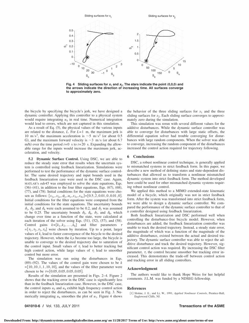
Fig. 4 Sliding surfaces for x1 and x2the arrows indicate the direction ofto approximately zero.

erically integrating u4 smoothes the plot of u1. Figure 4 shows

41010-6 / Vol. 133, JULY 2011


the behavior of the three sliding surfaces for x1 and the threesliding surfaces for x2. Each sliding surface converges to approxi-mately zero during the simulation.

This simulation was rerun with several different values for theadditive disturbances. While the dynamic surface controller wasable to converge for disturbances with large static offsets, thedifferential equation solver had trouble converging for distur-bances with large random components. When the solver was ableto converge, increasing the random component of the disturbancesincreased the control action required for trajectory following.

6 ConclusionsDSC, a robust nonlinear control technique, is generally applied

to mismatched systems in strict feedback form. In this paper, wedescribe a new method of defining states and state-dependent dis-turbances that allowed us to transform a nonlinear mismatcheddynamic system into strict feedback form. The method developedhere could be used for other mismatched dynamic systems requir-ing robust nonlinear control.

We applied this method to a MIMO extended-state kinematicmodel of a bicycle, which originally was not in strict feedbackform. After the system was transformed into strict feedback form,we were able to design a dynamic surface controller. We com-pared the performance of the dynamic surface controller to that ofa controller designed using feedback linearization.

Both feedback linearization and DSC performed well whencontrolling the disturbance-free bicycle model. However, whendisturbances are added, the feedback linearization controller wasunable to track the desired trajectory. Instead, a steady state error,the magnitude of which was a function of the magnitude of theadditive disturbance, existed between the actual and desired tra-jectory. The dynamic surface controller was able to reject the ad-ditive disturbance and track the desired trajectory. However, sig-nificant control action was required. By increasing the DSC filterparameter, , the control became smoother but tracking error in-creased. This demonstrates the trade-off between control actionand tracking error in all sliding controllers.

AcknowledgmentThe authors would like to thank Hope Weiss for her helpful

comments. J.L.M. was funded by a NDSEG fellowship.

References�1� Slotine, J. E., and Li, W., 1991, Applied Nonlinear Controls, Prentice-Hall,

050

100150 0

510

150

0.5

1

1.5

2

S4

Sliding surfaces for x2

S6

S2

e stars indicate the point „0,0,0… andreasing time. All surfaces converge

. Thinc

Englewood Cliffs, NJ.

Transactions of the ASME


J

Downloaded Fr

�2� Krstic, M., Kanellakopoulos, I., and Kokotovic, P., 1995, Nonlinear and Adap-tive Control Design, Wiley, New York.

�3� Won, M., and Hedrick, J. K., 1996, “Multiple-Surface Sliding Control of aClass of Uncertain Nonlinear Systems,” Int. J. Control, 64�4�, pp. 693–706.

�4� Swaroop, D., Hedrick, J. K., Yip, P. P., and Gerdes, J. C., 2000, “DynamicSurface Control for a Class of Nonlinear Systems,” IEEE Trans. Autom. Con-trol, 45�10�, pp. 1893–1899.

�5� Gomes, R. M. F., Sousa, J. B., and Pereira, F. L., 2003, “Integrated Maneuverand Control Design for ROV Operations,” Proc. IEEE OCEANS 2003, Vol. 2,pp. 703–710.

�6� Lu, X. Y., Tan, H. S., Shladover, S., and Hedrick, J. K., 2001, “NonlinearLongitudinal Controller Implementation and Comparison for AutomatedCars,” ASME J. Dyn. Syst., Meas., Control, 123�2�, pp. 161–167.

�7� Girard, A., and Hedrick, J. K., 2001, “Dynamic Positioning of Ships UsingNonlinear Dynamic Surface Control,” Proceedings of the Fifth IFAC Sympo-sium on Nonlinear Control Systems 2001.

�8� Yao, B., and Tomizuka, M., 1997, “Adaptive Robust Control of SISO Nonlin-ear Systems in a Semi-Strict Feedback Form,” Automatica, 33, pp. 893–900.

�9� Yao, B., and Tomizuka, M., 2001, “Adaptive Robust Control of MIMO Non-linear Systems in Semi-Strict Feedback Forms,” Automatica, 37, pp. 1305–1321.

�10� Getz, N., and Marsden, J., 1995, “Control for an Autonomous Bicycle,” Pro-ceedings of IEEE Conference on Robotics and Automation 1995, Vol. 2, pp.
1397–1402.


�11� Lee, S., and Ham, W., 2002, “Self Stabilizing Strategy in Tracking Control ofUnmanned Electric Bicycle With Mass Balance,” Proceedings of IEEE/RSJConference on Intelligent Robots and Systems 2002, Vol. 3, pp. 2200–2205.

�12� Astrom, K., Klein, R., and Lennartsson, A., 2005, “Bicycle Dynamics andControl: Adapted Bicycles for Education and Research,” IEEE Control Syst.Mag., 25�4�, pp. 26–47.

�13� Peng, H., and Tomizuka, M., 1990, “Vehicle Lateral Control for HighwayAutomation,” Proceedings of American Control Conference 1990, pp. 788–794.

�14� Hedrick, J. K., Tomizuka, M., and Varaiya, P., 1994, “Control Issues in Auto-mated Highway Systems,” IEEE Control Syst. Mag., 14�6�, pp. 21–32.

�15� Mathieu, J. L., and Hedrick, J. K., 2010, “Robust Multivariable DynamicSurface Control for Position Tracking of a Bicycle,” Proceedings of the Ameri-can Control Conference 2010, ACC-201-WeB11.1, pp. 1159–1165.

�16� Iuchi, K., Niki, H., and Murakami, T., 2005, “Attitude Control of BicycleMotion by Steering Angle and Variable COG Control,” Proceedings of IEEEIECON 2005, pp. 2065–2070.

�17� Isidori, A., 1995, Nonlinear Control Systems, Springer, New York.�18� Sastry, S., 1999, Nonlinear Systems: Analysis, Stability, and Control, Springer,

New York.�19� Song, B., Hedrick, J. K., and Howell, A., 2002, “Robust Stabilization and

Ultimate Boundedness of Dynamic Surface Control Systems via Convex Op-
timization,” Int. J. Control, 75�12�, pp. 870–881.
JULY 2011, Vol. 133 / 041010-7


transformation of a mismatched nonlinear dynamic system...

Documents