3

Transmission across

potential wells and

barriers

The physics of transmission and tunneling of waves and particles across differ-

ent media has wide applications. In geometrical optics, certain phenomenon

of light propagation cannot be explained without taking the wave nature of

light [51]. Thus interference, diffraction and ”tunnelling” of light through re-

gions which are forbidden in geometrical optics can be understood through

wave nature of light. Another example is the well-known phenomenon of to-

45

tal internal reflection. When light impinges upon the interface between two

media with refractive indices n1 and n2, it suffers total internal reflection when

θi ≥ sin−1(

n1n2

), where θi is the angle of incidence. According to the geometrical

optics description, there is no penetration of light into the rarer medium. How-

ever, it is known that, in reality, the light does propagate into the rarer medium,

even under total internal reflection conditions. This is possible by tunnelling

when the thickness of the rarer medium is comparable to the wavelength of

the light. The penetration of light into “forbidden” regions is used in a vari-

ety of optical devices such as prism couplers, directional couplers, switches,

etc. Similarly, in quantum mechanics the penetration of particle into forbidden

region can be explained by means of the wave nature associated with it.

The general problem of particle tunneling can be classified into two in-

teresting categories [51] both of which involve the propagation of a particle

with energy E through a classically forbidden region of potential energy V(x),

where E < V(x). In the first category, there is a region in space where the

particle can be represented by a “free” state and its energy is greater than the

background potential energy. As the particle strikes the barrier there will be a

finite probability of tunneling and a finite probability of being reflected back.

In the second category the particle is initially confined to a quantum well (ex-

ample: tunnelling through two or more barriers with wells in between). The

particle initially confined to a ”quantum well” region is a quasi-bound (QB) or

sharp resonant state. In the quasi-bound state, though the particle is primarily

confined to the quantum well, it has a finite probability of tunnelling out of the

well and escaping. The key differences between the two cases is that in the

first problem the wave function corresponding to the initial state is essentially

46

unbound, whereas in the second case it is primarily confined to the quantum

well region. However, the phenomenon of resonances is more general and can

occur during transmission across well, barrier, and potential pockets created by

two well separated barriers. These are generally outlined only briefly in some

of the books (see for example[52]) in literature. It may further be pointed out

that transmission and tunneling across potential barriers in one dimension is a

fundamental topic in the under graduate courses on quantum mechanics. But,

most of the text books on introductory quantum mechanics confine to trans-

mission and tunneling across the potential barriers and approximate methods

to calculate the transmission coefficients using WKB type approximation (see

for example [31]). Similarly resonance tunneling is briefly outlined by indicat-

ing the reflectionless transmission at specific energies . Therefore, a systematic

study [11, 12] of resonant or quasi-bound states, their widths, and their relation

to the variation of T is desirable.

S -matrix theory in three dimensional (3D) potential scattering provides a

unified way for the analysis of resonances and bound states generated by the

potential through its analytical structure [10]. These are done using the study of

pole structure of S -matrix in complex momentum or complex energy planes. In

chapter 2 we have outlined how a somewhat similar procedure can be adopted

in one dimensional transmission problem using the pole structure of reflec-

tion amplitude and transmission amplitude. In three-dimensional systems, a

potential with an attractive well followed by a barrier is useful for analyzing

bound states, sharp resonances generated by potential pockets, and broader or

above barrier resonant states generated by wide barriers [53]. In contrast, in

one dimension we usually study a set of two or more well separated potential

47

barriers [12, 54]. The gap between two adjacent potential barriers provides

a pocket for the formation of sharp resonant states, and these generate sharp

peaks in the transmission coefficient. In addition, ordinary potential wells and

barriers can also generate resonances but they will be broader. It is also impor-

tant to study the resonance generated by purely attractive well. The motivation

of the present chapter is to explore the nature of broader resonances and related

subtle features of the transmission across purely attractive well and the corre-

sponding repulsive barrier to obtain a deeper understanding of transmission

across a potential in one dimension. The study of sharper quasi-bound states

[12] generated by twin symmetric barriers will be described in next chapter.

This chapter (see ref. [11]) is organized as follows: Section 3.1 is about the

formulation of bound states, resonant states and transmission coefficient T in

1D. In section 3.2 we investigate the resonance states, its correlation with os-

cillatory structure of T and the corresponding box potential for 1D rectangular

potential. In section 3.3 we study the transmission across a potential having

a combination of well and barrier and in section 3.4 we analyze T across an

attractive potential for which T does not show any oscillations. In section 3.5

we summarize the main conclusions of our study.

3.1 Bound states, resonance states and

transmission coefficient

The basic equation that we use to study the bound states, resonant states, trans-

mission and reflection is the one dimensional time independent Schrodinger

48

equation for a particle of mass m with potential U(x) and total energy E:

d2ϕ(x)dx2 + (k2 − V(x))ϕ(x) = 0, (3.1)

where k2 = 2mE/~2, V(x) = 2mU(x)/~2 and α2 = k2 − V(x). For convenience

we use the units 2m = 1 and ~2=1 such that k2 denotes energy E. In our

numerical calculations we have used Å as the unit of length and Å−2 as the

unit of energy.

(a) Bound state eigenvalues from bound state wave function

Stationary states of the system which correspond to discrete energy levels and

describe the bound state motion are called bound states. For bound states,

the energy is real and its wave function is square integrable. If a potential

can generate bound states, then the solution of Eq.(3.1) have exponentially

decaying tails at the boundaries. For potentials vanishing as |x| → ∞, the bound

state energies are negative. In particular, for short-range potentials satisfying

plane wave or free particle asymptotic boundary conditions, the bound state

wave function has the asymptotic behavior:

ϕ(x) −→|x|→∞

e−kb |x|, (3.2)

and the corresponding bound state energy Eb is given by Eb = (ikb)2 = −k2b .

We see that the bound states can be thought of as negative energy states with

zero width.

(b) Resonance state eigenvalues from resonance state wave function

For evaluation of the resonant states, we seek a solution of Eq.(3.1) with

complex energy k2R = (kr − iki)2 = (k2

r − k2i ) − i2krki = ER = Er − iΓr/2 with

49

Er > 0 and Γr > 0 such that the wave function behaves asymptotically as:

ϕ(x) −→x→∞

ei(kr−iki)x

ϕ(x) −→x→−∞

e−i(kr−iki)x. (3.3)

This behavior implies a positive energy state Er with width Γr and lifetime ~/Γr

and |ϕ(x)| diverges exponentially as eki |x| but decays exponentially in time be-

cause the time-dependent part of the solution of the Schrodinger wave equation

is e−iEt/~. Smaller width Γr corresponds to a long lived resonance state. If the

widths are very narrow, resonant states behave similarly to bound states in the

vicinity of the potential and may be considered as QB state. However, unlike

the bound states the QB or resonance states are not normalizable because of

the exponential divergence stated above indicating the significant presence of

resonance state wave function in the entire domain.

(c) Resonance states and transmission coefficient

In one dimensional quantum transmission across a potential, the transmission

coefficient can be obtained by solving the Schrodinger wave equation for E > 0

and then by applying the appropriate boundary conditions for the continuity of

ϕ(x) and ϕ′(x) at the boundaries. A smooth potential can be approximated by

a large number of very small step potentials, and the transmission and reflec-

tion coefficient R can be obtained by using transfer matrix technique. This

method can be used for potentials that are not analytically solvable. Alterna-

tively, one can adopt a numerical integration of the Schrodinger equation using

well known procedures like Runge kutta method.

50

For the study of R and T we seek a solution of ϕ(x) satisfying the conditions:

ϕ(x) −→x→−∞

Aeikx + Be−ikx,

ϕ(x) −→x→∞

Feikx, (3.4)

such that T = |F/A|2 and R = |B/A|2, where A, B and F are amplitudes of

incident, reflected and transmitted wave respectively. In one dimension scat-

tering potential, the S -matrix is given by the ratio of F/A. The pole of F/A

in the complex k-plane or in the complex energy E-plane generated by zero of

A corresponds to the resonant state. The resonance state energy generated by

the potential can be estimated from T by studying it as a function of energy E.

In the vicinity of resonance, T shows peaks due to enhanced transmission at

resonance energy. The peak position of T corresponds to resonance energy Er

and its width corresponds to the width of the resonance state Γr.

3.2 Resonance states and transmission generated

by rectangular potential

As a simple analytically solvable example, we consider the attractive square

well potential of width 2a given by:

V(x) =

−V0, V0 > 0, |x| < a,

0, |x| > a.(3.5)

51

The corresponding box potential of attractive square well potential is:

V(x) =

−V0, V0 > 0, |x| < a,

∞, |x| > a,(3.6)

which generates the eigenvalues:

En = −V0 + n2π2/(2a)2, n = 1, 2, ..... (3.7)

The potential in Eq.(3.6) can be considered to be infinitely repulsive for |x| > a,

we expect that the states for E < 0 have higher energies than the corresponding

square well given by Eq.(3.5). These potentials can generate bound and reso-

nance states. Since the potential V(x) is symmetric in x, the states generated

will have definite parity.

• The resonance state positions and widths are evaluated by solving the

Schrodinger equation Eq.(3.1), satisfying the boundary conditions given

by Eq.(3.3). Because we have chosen the potential to be symmetric with

respect to the origin, we expect both even and odd wave functions. The

former behave as cos(αx) near the origin and the latter as sin(αx). Thus

for even resonant states, the matching of the wave function and its deriva-

tive at x = a leads to the condition αtan(αa) = −ik. As a result the even

resonance state energy and widths are obtained from the complex roots

kn of the equation:

kcos(αa) − iαsin(αa) = 0. (3.8)

52

The roots kn are just below the real k-axis in the complex k-plane such

that Re(kn) > |Im(kn)|. This condition signifies a positive energy resonant

state with finite width. The corresponding equation for the energies and

widths of odd states is:

ksin(αa) + iαcos(αa) = 0. (3.9)

By incorporating the asymptotic condition Eq.(3.2), a similar procedure

can be used to obtain the bound state energy eigenvalues En.

• The transmission and reflection coefficient generated by the attractive

rectangular potential Eq.(3.5) is obtained by solving the Eq.(3.1) with

boundary condition given by Eq.(3.4). The following expressions are

obtained [23]:

FA=

4αke−2ika

(α + k)2e−2iαa − (α − k)2e2iαa , (3.10)

BA= −2i

(k2 − α2)4kα

sin(2αa)e2ika

(FA

), (3.11)

BA=

2i(α2 − k2)sin(2αa)[e−2iαa(α + k)2 − e2iαa(α − k)2]

, (3.12)

BF=

2i(α2 − k2)sin(2αa)4kα

, (3.13)

T =

∣∣∣∣∣∣FA∣∣∣∣∣∣2 = (4αk)2

(4kα)2 + 4(α2 − k2)2sin2(2αa), (3.14)

53

R =

∣∣∣∣∣∣BA∣∣∣∣∣∣2 = 4(α2 − k2)2sin2(2αa)

(4kα)2 + 4(α2 − k2)2sin2(2αa)= 1 − T, (3.15)

where α2 = V0 + k2. For a repulsive rectangular potential α2 = k2 − V0.

3.2.1 Comparison of the states generated by an attractive

square potential and the corresponding box potential

We evaluate the eigenstates generated by the potential given by Eq.(3.5) by

solving Eq.(3.1) satisfying the boundary condition Eq.(3.3) for resonance states

and Eq.(3.2) for bound states and compare these eigenstates with the corre-

sponding box potential Eq.(3.6). The eigenstates generated by the potential

Eq.(3.5) is also examined from the oscillatory structure of T as a function of

energy. The oscillatory behavior of T is due to the sine term in Eq.(3.14). In

Figure. 3.1 we show the variation of T with energy for a set of potential pa-

rameters. As E → ∞, T → 1 as it should. In our numerical calculations we

use Å as the unit of length and Å−2 as the unit of energy (i.e we set 2m = 1,

~ = 1), and choose parameters such that the numerical results and figures show

the physical features we seek to highlight. In Table 3.1 we summarize the nu-

merical results obtained using V0 = −3 and a = 5. In this case the attractive

square well has six bound states, and the corresponding box potential has only

five negative energy states. We also give the positions of the peaks of T . From

Table 3.1 it is clear that the peaks positions of T are related to the energies

of the corresponding resonant states, even though there is a small difference

in the numerical values. This difference is primarily due to the large widths

associated with the resonances generated by attractive well.

54

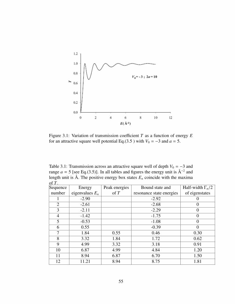
Figure 3.1: Variation of transmission coefficient T as a function of energy Efor an attractive square well potential Eq.(3.5 ) with V0 = −3 and a = 5.

Table 3.1: Transmission across an attractive square well of depth V0 = −3 andrange a = 5 [see Eq.(3.5)]. In all tables and figures the energy unit is Å−2 andlength unit is Å. The positive energy box states En coincide with the maximaof T .Sequence Energy Peak energies Bound state and Half-width Γn/2number eigenvalues En of T resonance state energies of eigenstates

1 -2.90 -2.92 02 -2.61 -2.68 03 -2.11 -2.29 04 -1.42 -1.75 05 -0.53 -1.08 06 0.55 -0.39 07 1.84 0.55 0.46 0.308 3.32 1.84 1.72 0.629 4.99 3.32 3.18 0.9110 6.87 4.99 4.84 1.2011 8.94 6.87 6.70 1.5012 11.21 8.94 8.75 1.81

55

Figure 3.2: Comparison of bound and resonant states of an attractive squarewell in Eq.(3.5) for potential parameters V0 = −3 and a = 5 with the corre-sponding states for the box potential (3.6). The abscissa is the sequence num-ber of the states. It may be pointed out that in the case of the bound states ofattractive square well n−1 signifies the ‘principal’ quantum number associatedwith energy eigenvalues.

In Figure.3.2 we demonstrate a correlation between the bound and reso-

nance states of the attractive square well and the corresponding box energy

eigenvalues given by Eq.(3.7). Along the x-axis we give the sequence number

of the resonant states and bound states generated by the box, as they occur,

starting with the lowest energy state. These numbers can be interpreted as

quantum numbers for the bound states. From Table 3.1 we see that the sets of

positive energy states generated by the potential in Eq.(3.5) and the peak posi-

tions of T for the corresponding well are the same, but the results for negative

energy bound states for the potential given by Eq.(3.5) and the corresponding

results for the box potential differ.

56

Correlation between peaks of T and the resonance states

It is well known that in 3D potential scattering the bound states and resonant

states can be associated with the poles of the S -matrix in complex k or, equiv-

alently, complex-E plane [10]. For transmission across a potential in one di-

mension, it is natural to examine whether the resonant states we have described

correspond to the complex poles of the transmission amplitude F/A. From Eq.

(3.11) we see that the pole structure of F/A and the reflection amplitude B/A

are the same. The only condition to be satisfied is that for real positive energies

R + T = 1, which means that whenever T has a peak R has a minimum. If we

use Eq.(3.11) for F/A and a convenient numerical procedure such as an itera-

tive method, we can calculate the zeros of the denominator of Eq.(3.10), which

will generate the poles of F/A and B/A. From this calculation we can verify

that all the resonance states listed in Table 3.1 correspond to the complex poles

of F/A.

The reason for relating the complex poles of F/A to resonances are as follows:

The amplitude A/F can be understood as the coefficient of an incoming inci-

dent wave eikx as x→ −∞ when the outgoing transmitted wave eikx for x→ ∞

has amplitude unity. Similarly, B/F can be understood as the coefficient of the

reflected wave as x → −∞ for the same condition. If A/F = 0 for a complex

k = kr − iki in the lower half of k-plane with kr > ki, the resulting wave func-

tion satisfies the asymptotic condition given in Eq.(3.3) signifying a resonant

state. However, A/F = 0 implies a corresponding pole in F/A, signifying that

F/A has complex poles corresponding to a resonance. This correspondence

is analogous to three dimensional potential scattering for which the complex

zeros k = kr − iki of the coefficient of incoming spherical wave component of

57

the regular solution of the scattering problem represent the resonant states and

consequently are identified as the pole position of the corresponding partial

wave S -matrix S l [10]. This result demonstrates that resonances have similar

interpretations in one and three dimensions. If let A/F = 0, we obtain the

condition satisfied by the zeros of A/F:

α + kα − k

= ±e2iαa , (3.16)

which corresponds to the complex poles of the transmission amplitude F/A.

It is straightforward to verify that Eq.(3.16) implies Eqs.(3.8) and (3.9), which

generate the resonance energies and widths. This verification and the numerical

example we have described demonstrate that the complex poles of the trans-

mission amplitude F/A for unit incident wave signify resonances and generate

the peaks of the oscillations of T for an attractive square well potential.

3.2.2 Numerical analysis of resonance states generated by

repulsive rectangular potential and its corresponding

box potential

For our study of resonance states generated by a repulsive potential, we have

taken a repulsive rectangular potential of width 2a given by:

V(x) =

V0, V0 > 0, |x| < a,

0, |x| > a .(3.17)

58

The corresponding box potential is:

V(x) =

V0, V0 > 0, |x| < a,

∞, |x| > a ,(3.18)

which can generate the eigenvalues:

En = V0 + n2π2/(2a)2, n = 1, 2, ..... (3.19)

Transmission across such a potential is the most commonly studied example in

introductory quantum mechanics. Our primary interest is in the interpretation

of the oscillations of T for energies E > V0 with the resonance states generated

by the potential Eq.(3.17). In Figure. 3.3 we show the variation of T with E

for the potential Eq.(3.17). Based on our interpretation of the oscillations of

T generated by an attractive square well, we can understand these oscillations

in a similar manner. Resonances generated by a reasonably flat barrier are

well studied for nucleus-nucleus collisions [53, 55]. Barrier top resonances are

broader states compared to the very narrow resonant states that are generated

by the potential pockets sandwiched between wide barriers. However if the

barrier is flatter and wider, a number of narrower resonance states are generated

for energies above the barrier. This condition is satisfied in our example of the

rectangular barrier with the choice a = 5. Unlike the attractive well, there are

no bound states associated with the rectangular barrier in Eq.(3.17).

We used the conditions given in Eq.(3.3) to search for resonance states gen-

erated by the barrier at energies E > V0. These states along with the maxima

of T are listed in Table 3.2. The expression T for E < V0 is given by Eq.(3.14)

59

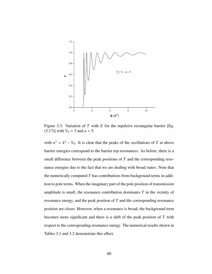
Figure 3.3: Variation of T with E for the repulsive rectangular barrier [Eq.(3.17)] with V0 = 3 and a = 5.

with α2 = k2 − V0. It is clear that the peaks of the oscillations of T at above

barrier energies correspond to the barrier top resonances. As before, there is a

small difference between the peak positions of T and the corresponding reso-

nance energies due to the fact that we are dealing with broad states. Note that

the numerically computed T has contributions from background terms in addi-

tion to pole terms. When the imaginary part of the pole position of transmission

amplitude is small, the resonance contribution dominates T in the vicinity of

resonance energy, and the peak position of T and the corresponding resonance

position are closer. However, when a resonance is broad, the background term

becomes more significant and there is a shift of the peak position of T with

respect to the corresponding resonance energy. The numerical results shown in

Tables 3.1 and 3.2 demonstrate this effect.

60

To make the comparison between the attractive well and the corresponding

barrier more complete, we examine the variation of the barrier top resonance

position En with n and compare it with the corresponding box potential posi-

tive energy eigenvalues Eq.(3.19). We show this in Figure 3.4. The correlation

between the box states and barrier top states is close as in the case for an attrac-

tive square well. Figure 3.2 looks different because of the single sequencing

of bound and resonant states generated by the well. The positive energy states

generated by Eq.(3.17) and the corresponding peak position of T match very

well. The reason for this common feature can be understood as follows.

The expression for T in Eq.(3.14) holds for an attractive square well with

α2 = k2 + V0. The same expression is valid for the barrier for k2 > V0 with

α2 = k2 − V0. We have taken the width 2a of the well and the barrier to be

large (a = 5) to generate a greater number of states. For both the well and

the barrier, the maxima of T are governed by the zeros of sin(2αa). Thus for

an attractive well, the peaks of T are at positive energies, signifying that the

resonances occur at En = [(n2π2/(2a)2) − V0] > 0. Such a close correlation is

not present for the negative energy states, as is clear from Table 3.1. For the

barrier, the peaks of T are at En = [(n2π2/(2a)2) + V0] for n=1,2,.... Both sets

of En are eigenvalues of the corresponding box potentials. In contrast, resonant

state energies and widths are generated from the complex poles of T , and their

positions are slightly shifted from the maxima of T because the resonances are

broader. Tables 3.1 and 3.2 summarize these results.

61

Table 3.2: Comparison of transmission peaks and barrier resonance energiesfor the square barrier potential Eq. (3.17) with V0 = 3 and a = 5.

Sequence Energy eigenvalues Peak energy Resonance Resonancenumber n En of T energies Er half-width Γr/2

1 3.10 3.10 3.10 0.022 3.40 3.40 3.38 0.093 3.89 3.89 3.86 0.194 4.58 4.58 4.53 0.335 5.47 5.47 5.40 0.506 6.55 6.55 6.46 0.707 7.84 7.84 7.72 0.928 9.32 9.32 9.19 1.16

Figure 3.4: Comparison of the barrier top resonant state energies of the repul-sive rectangular potential [Eq. 3.17] with V0 = 3 and a = 5 with the corre-sponding states for the box potential [Eq. 3.18]. The abscissa is the sequencenumber of the states.

62

3.3 Effect of adjacent well on barrier

transmission

Now we wish to discuss an interesting aspect of barrier tunneling. In most

applications for studying the transmission probability across a potential bar-

rier one uses the well known barrier penetration formula deduced using WKB

approximation. In this approximation, one explores only the barrier region of

the potential between classical turning points and the rest of the potential on

either side of the barrier play no role. This cannot be strictly true because, in

principle, transmission and tunneling should depend on the the full potential.

In particular if there is a deep well on either or both sides of the barrier, the

resonances generated by these states can be expected to affect the behaviour of

T . This feature was explored earlier in Ref.[14]. In this section we demonstrate

the role of adjacent well in the transmission across a rectangular barrier having

an attractive well on one side. The WKB approximation based expression for

T is given by (see also Eq.(2.60)):

T = exp[− 2

x2∫x1

√(V(x) − k2)dx

]. (3.20)

Here x1 and x2 > x1 are the turning points, which define the classically forbid-

den region x1 < x < x2 of the barrier at E = k2.

This semiclassical approach to tunneling incorporates the potential between

the turning points at a given energy but ignores the potential elsewhere result-

ing in the expression for T given by Eq.(3.20), which is independent of V(x) in

the domains x < x1 and x > x2. In the light of our discussion on the transmis-

63

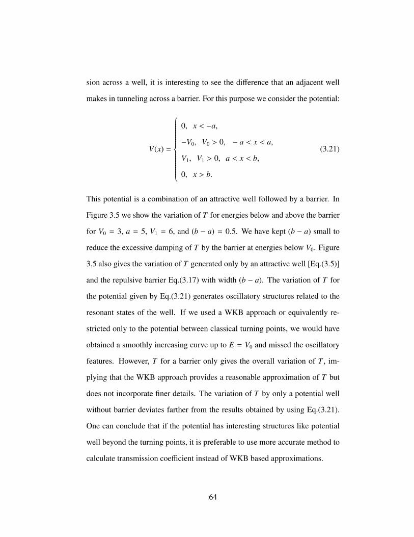
sion across a well, it is interesting to see the difference that an adjacent well

makes in tunneling across a barrier. For this purpose we consider the potential:

V(x) =

0, x < −a,

−V0, V0 > 0, − a < x < a,

V1, V1 > 0, a < x < b,

0, x > b.

(3.21)

This potential is a combination of an attractive well followed by a barrier. In

Figure 3.5 we show the variation of T for energies below and above the barrier

for V0 = 3, a = 5, V1 = 6, and (b − a) = 0.5. We have kept (b − a) small to

reduce the excessive damping of T by the barrier at energies below V0. Figure

3.5 also gives the variation of T generated only by an attractive well [Eq.(3.5)]

and the repulsive barrier Eq.(3.17) with width (b − a). The variation of T for

the potential given by Eq.(3.21) generates oscillatory structures related to the

resonant states of the well. If we used a WKB approach or equivalently re-

stricted only to the potential between classical turning points, we would have

obtained a smoothly increasing curve up to E = V0 and missed the oscillatory

features. However, T for a barrier only gives the overall variation of T , im-

plying that the WKB approach provides a reasonable approximation of T but

does not incorporate finer details. The variation of T by only a potential well

without barrier deviates farther from the results obtained by using Eq.(3.21).

One can conclude that if the potential has interesting structures like potential

well beyond the turning points, it is preferable to use more accurate method to

calculate transmission coefficient instead of WKB based approximations.

64

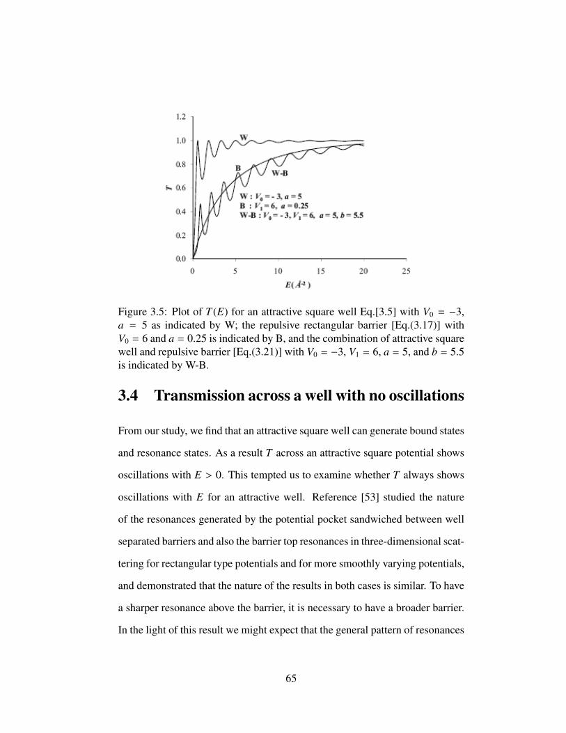
Figure 3.5: Plot of T (E) for an attractive square well Eq.[3.5] with V0 = −3,a = 5 as indicated by W; the repulsive rectangular barrier [Eq.(3.17)] withV0 = 6 and a = 0.25 is indicated by B, and the combination of attractive squarewell and repulsive barrier [Eq.(3.21)] with V0 = −3, V1 = 6, a = 5, and b = 5.5is indicated by W-B.

3.4 Transmission across a well with no oscillations

From our study, we find that an attractive square well can generate bound states

and resonance states. As a result T across an attractive square potential shows

oscillations with E > 0. This tempted us to examine whether T always shows

oscillations with E for an attractive well. Reference [53] studied the nature

of the resonances generated by the potential pocket sandwiched between well

separated barriers and also the barrier top resonances in three-dimensional scat-

tering for rectangular type potentials and for more smoothly varying potentials,

and demonstrated that the nature of the results in both cases is similar. To have

a sharper resonance above the barrier, it is necessary to have a broader barrier.

In the light of this result we might expect that the general pattern of resonances

65

we have found for the attractive rectangular well and rectangular barrier is ap-

plicable even when they are replaced by smoother potentials. However there

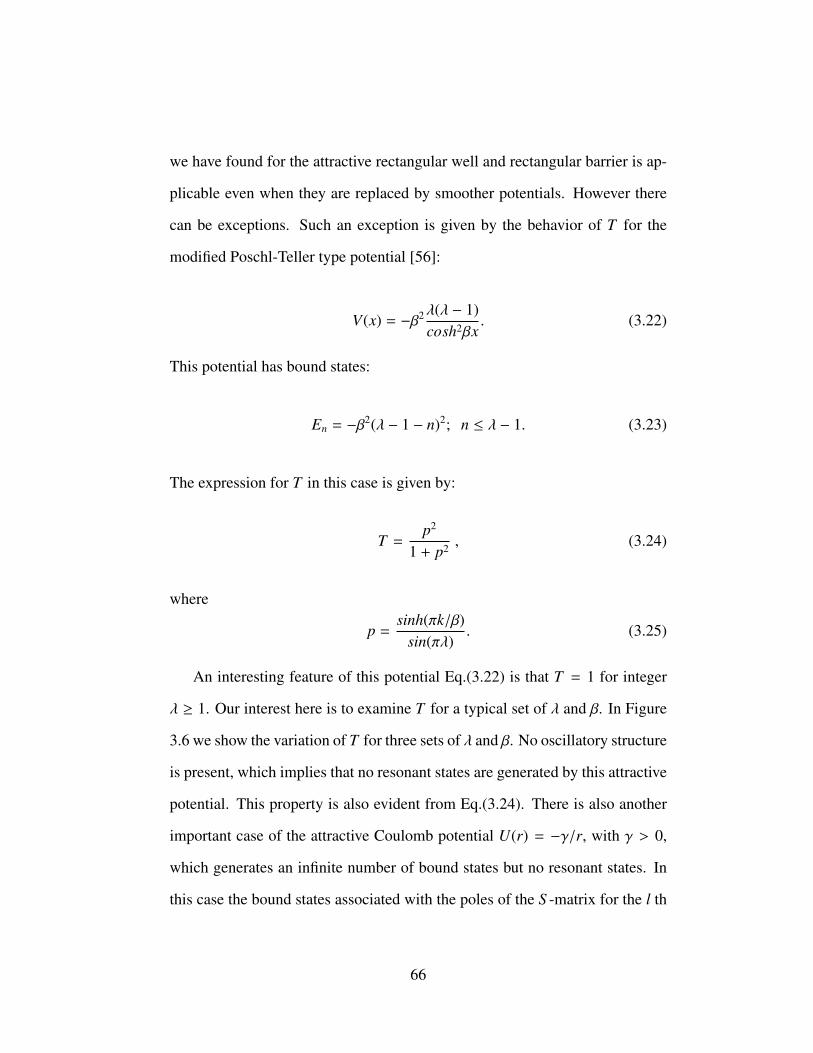
can be exceptions. Such an exception is given by the behavior of T for the

modified Poschl-Teller type potential [56]:

V(x) = −β2λ(λ − 1)cosh2βx

. (3.22)

This potential has bound states:

En = −β2(λ − 1 − n)2; n ≤ λ − 1. (3.23)

The expression for T in this case is given by:

T =p2

1 + p2 , (3.24)

where

p =sinh(πk/β)

sin(πλ). (3.25)

An interesting feature of this potential Eq.(3.22) is that T = 1 for integer

λ ≥ 1. Our interest here is to examine T for a typical set of λ and β. In Figure

3.6 we show the variation of T for three sets of λ and β. No oscillatory structure

is present, which implies that no resonant states are generated by this attractive

potential. This property is also evident from Eq.(3.24). There is also another

important case of the attractive Coulomb potential U(r) = −γ/r, with γ > 0,

which generates an infinite number of bound states but no resonant states. In

this case the bound states associated with the poles of the S -matrix for the l th

66

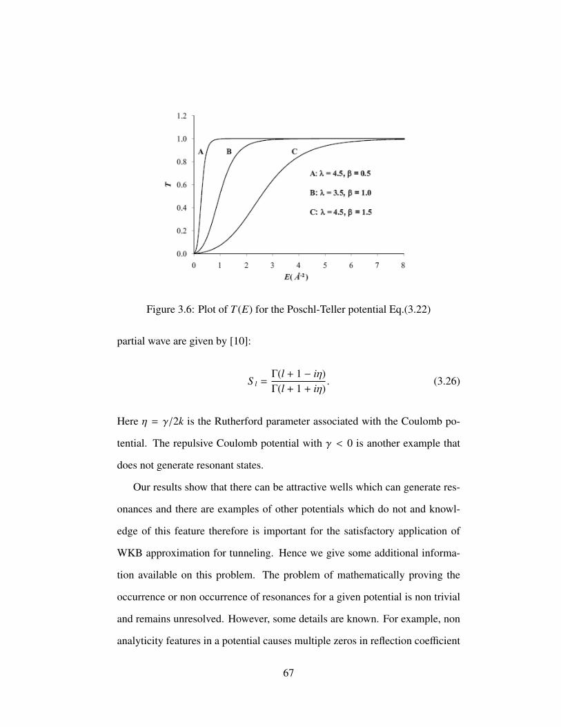
Figure 3.6: Plot of T (E) for the Poschl-Teller potential Eq.(3.22)

partial wave are given by [10]:

S l =Γ(l + 1 − iη)Γ(l + 1 + iη)

. (3.26)

Here η = γ/2k is the Rutherford parameter associated with the Coulomb po-

tential. The repulsive Coulomb potential with γ < 0 is another example that

does not generate resonant states.

Our results show that there can be attractive wells which can generate res-

onances and there are examples of other potentials which do not and knowl-

edge of this feature therefore is important for the satisfactory application of

WKB approximation for tunneling. Hence we give some additional informa-

tion available on this problem. The problem of mathematically proving the

occurrence or non occurrence of resonances for a given potential is non trivial

and remains unresolved. However, some details are known. For example, non

analyticity features in a potential causes multiple zeros in reflection coefficient

67

[57]. Similarly the top/bottom curvature and higher localization of a potential

profile can be crucial in generating resonances [58]. More interestingly the

rectangular well/barrier seems to be the best illustration which displays these

oscillations. On the other hand potentials like Gaussian, Lorentzian, exponen-

tial, parabolic or Eckart do not entail multiple oscillations in T as they are less

localized. The WKB formula for R and T works well for them. Higher order

potential like V(x) = −V0x2n,±V0e−x2n, ±,V0

1+x2n , n=2,3,4... can become reflection-

less at certain discrete energies [58, 59].

3.5 Summary

Now we summarize below the main conclusions about our study of quantum

transmission and eigenstates generated by potentials like wells and barriers:

• By taking an attractive square well and its repulsive counterpart, we have

shown that the oscillations in T as a function of energy corresponds to

the broad resonant state energies obtained by using boundary conditions

satisfied by the resonant state wave function.

• We found that the resonant energies and their widths can be obtained in

terms of the complex poles of the transmission amplitude or reflection

amplitude in the lower half of the complex E-plane in the vicinity of

the real axis. This result is similar to the corresponding behavior of S -

matrix poles in three-dimensional scattering and hence provides a unified

understanding of transmission in one dimension and potential scattering

in three dimensions in terms of the pole structure of the corresponding

amplitudes.

68

• For an attractive square well and the rectangular barrier, the positions of

the maxima of T are practically same as the energies of the eigenstates of

the corresponding one-dimensional box potentials. The resonance state

energies are also close to the peak positions of T , this confirms the close

correlation between the oscillatory structure of T at resonance energies.

• From the study of transmission across a potential that is a combination

of an attractive well and a repulsive barrier, we found that T exhibits os-

cillations even at energies below the barrier, in contrast to the WKB type

barrier expression for T , which does not manifest these features. Hence

simple WKB type expressions for T may not be a reasonable approxima-

tion if the total potential has physical features such as an attractive well

outside the barrier region.

• The oscillations of T across an attractive potential are likely to be found

for most potentials. But these features can have exceptions for example

the attractive modified Poschl-Teller type potential which can generate

bound states but no resonance states. Hence the study of T across this

potential as a function of energy does not show any oscillations.

69