transportation conformity guidance for … december 2010 transportation and regional programs...

Transportation Conformity Guidance for Quantitative Hot-spot Analyses in PM2.5 and PM10 Nonattainment and Maintenance Areas

EPA-420-B-10-040 December 2010

Transportation and Regional Programs Division Office of Transportation and Air Quality U.S. Environmental Protection Agency

Transportation Conformity Guidance for Quantitative Hot-spot Analyses in PM2.5 and PM10 Nonattainment and

Maintenance Areas

i

LIST OF EXHIBITS .................................................................................................................................... V

Table of Contents

LIST OF APPENDICES .............................................................................................................................. V

SECTION 1: INTRODUCTION ................................................................................................................. 1

1.1 PURPOSE OF THIS GUIDANCE.................................................................................................... 1 1.2 TIMING OF QUANTITATIVE PM HOT-SPOT ANALYSES ................................................................ 1 1.3 DEFINITION OF A HOT-SPOT ANALYSIS ..................................................................................... 2 1.4 PROJECTS REQUIRING A PM HOT-SPOT ANALYSIS ..................................................................... 2 1.5 OTHER PURPOSES FOR THIS GUIDANCE .................................................................................... 3 1.6 ORGANIZATION OF THIS GUIDANCE ......................................................................................... 3 1.7 ADDITIONAL INFORMATION ..................................................................................................... 4 1.8 GUIDANCE AND EXISTING REQUIREMENTS .............................................................................. 5

SECTION 2: TRANSPORTATION CONFORMITY REQUIREMENTS............................................. 6

2.1 INTRODUCTION ........................................................................................................................ 6 2.2 OVERVIEW OF STATUTORY AND REGULATORY REQUIREMENTS ............................................... 6 2.3 INTERAGENCY CONSULTATION AND PUBLIC PARTICIPATION REQUIREMENTS .......................... 8 2.4 HOT-SPOT ANALYSES ARE BUILD/NO-BUILD ANALYSES ........................................................... 9

2.4.1 General ................................................................................................................................... 9 2.4.2 Suggested approach for PM hot-spot analyses ....................................................................... 9 2.4.3 Guidance focuses on refined PM hot-spot analyses ..............................................................11

2.5 EMISSIONS CONSIDERED IN PM HOT-SPOT ANALYSES..............................................................13 2.5.1 General requirements ............................................................................................................13 2.5.2 PM emissions from motor vehicle exhaust, brake wear, and tire wear .................................13 2.5.3 PM2.5 emissions from re-entrained road dust .........................................................................13 2.5.4 PM10 emissions from re-entrained road dust .........................................................................13 2.5.5 PM emissions from construction-related activities ................................................................14

2.6 NAAQS CONSIDERED IN PM HOT-SPOT ANALYSES ...................................................................14 2.7 BACKGROUND CONCENTRATIONS...........................................................................................14 2.8 APPROPRIATE TIME FRAME AND ANALYSIS YEARS .................................................................15 2.9 AGENCY ROLES AND RESPONSIBILITIES ..................................................................................16

2.9.1 Project sponsor ......................................................................................................................16 2.9.2 DOT .......................................................................................................................................16 2.9.3 EPA ........................................................................................................................................16 2.9.4 State and local transportation and air agencies ....................................................................16

SECTION 3: OVERVIEW OF A QUANTITATIVE PM HOT-SPOT ANALYSIS .............................18

3.1 INTRODUCTION .......................................................................................................................18 3.2 DETERMINE NEED FOR A PM HOT-SPOT ANALYSIS (STEP 1) .....................................................18 3.3 DETERMINE APPROACH, MODELS, AND DATA (STEP 2) ............................................................18

3.3.1 General ..................................................................................................................................18 3.3.2 Determining the geographic area and emission sources to be covered by the analysis ........20 3.3.3 Deciding the general analysis approach and analysis year(s) ..............................................20 3.3.4 Determining the PM NAAQS to be evaluated ........................................................................21 3.3.5 Deciding on the type of PM emissions to be modeled ............................................................22 3.3.6 Determining the models and methods to be used ...................................................................22 3.3.7 Obtaining project-specific data .............................................................................................22

3.4 ESTIMATE ON-ROAD MOTOR VEHICLE EMISSIONS (STEP 3) ......................................................23 3.5 ESTIMATE EMISSIONS FROM ROAD DUST, CONSTRUCTION, AND ADDITIONAL SOURCES (STEP 4) ...................................................................................................................................23 3.6 SELECT AN AIR QUALITY MODEL, DATA INPUTS AND RECEPTORS (STEP 5) ..............................23 3.7 DETERMINE BACKGROUND CONCENTRATIONS FROM NEARBY AND OTHER SOURCES

(STEP 6) ...................................................................................................................................24

ii

3.8 CALCULATE DESIGN VALUES AND DETERMINE CONFORMITY (STEP 7) ....................................24 3.9 CONSIDER MITIGATION OR CONTROL MEASURES (STEP 8) .......................................................25 3.10 DOCUMENT THE PM HOT-SPOT ANALYSIS (STEP 9) ..................................................................25

SECTION 4: ESTIMATING PROJECT-LEVEL PM EMISSIONS USING MOVES ........................27

4.1 INTRODUCTION .......................................................................................................................27 4.2 CHARACTERIZING A PROJECT IN TERMS OF LINKS ...................................................................29

4.2.1 Highway and intersection projects ........................................................................................30 4.2.2 Transit and other terminal projects .......................................................................................32

4.3 DETERMINING THE NUMBER OF MOVES RUNS .........................................................................32 4.3.1 General ..................................................................................................................................32 4.3.2 Projects with typical travel activity data ...............................................................................34 4.3.3 Projects with additional travel activity data ..........................................................................35

4.4 DEVELOPING BASIC RUN SPECIFICATION INPUTS.....................................................................35 4.4.1 Description ............................................................................................................................36 4.4.2 Scale ......................................................................................................................................36 4.4.3 Time Spans .............................................................................................................................37 4.4.4 Geographic Bounds ...............................................................................................................37 4.4.5 Vehicles/Equipment ...............................................................................................................37 4.4.6 Road Type ..............................................................................................................................38 4.4.7 Pollutants and Processes .......................................................................................................39 4.4.8 Manage Input Data Sets ........................................................................................................40 4.4.9 Strategies ...............................................................................................................................40 4.4.10 Output ....................................................................................................................................41 4.4.11 Advanced Performance Features...........................................................................................41

4.5 ENTERING PROJECT DETAILS USING THE PROJECT DATA MANAGER ........................................42 4.5.1 Meteorology ...........................................................................................................................43 4.5.2 Age Distribution ....................................................................................................................44 4.5.3 Fuel Supply and Fuel Formulation ........................................................................................45 4.5.4 Inspection and Maintenance (I/M) ........................................................................................45 4.5.5 Link Source Type ...................................................................................................................45 4.5.6 Links ......................................................................................................................................46 4.5.7 Describing Vehicle Activity ...................................................................................................46 4.5.8 Deciding on an approach for activity ....................................................................................48 4.5.9 Off-Network ...........................................................................................................................48

4.6 GENERATING EMISSION FACTORS FOR USE IN AIR QUALITY MODELING ..................................50 4.6.1 Highway and intersection links..............................................................................................50 4.6.2 Transit and other terminal links ............................................................................................51

SECTION 5: ESTIMATING PROJECT-LEVEL PM EMISSIONS USING EMFAC (IN CALIFORNIA) ............................................................................................................................................52

5.1 INTRODUCTION .......................................................................................................................52 5.2 CHARACTERIZING A PROJECT IN TERMS OF LINKS ...................................................................54

5.2.1 Highway and intersection projects ........................................................................................54 5.2.2 Transit and other terminal projects .......................................................................................55

5.3 DETERMINING THE NUMBER OF EMFAC RUNS .........................................................................56 5.4 DEVELOPING BASIC SCENARIO INPUTS ....................................................................................58

5.4.1 Geographic area and calculation method .............................................................................58 5.4.2 Calendar year ........................................................................................................................59 5.4.3 Season or month ....................................................................................................................59 5.4.4 Scenario title ..........................................................................................................................59 5.4.5 Model years ...........................................................................................................................59 5.4.6 Vehicle classes .......................................................................................................................60 5.4.7 I/M program schedule and other state control measures ......................................................60

5.5 CONFIGURING EMISSION FACTOR OUTPUTS ............................................................................61 5.5.1 Temperature and relative humidity ........................................................................................61

iii

5.5.2 Speed......................................................................................................................................62 5.5.3 Output rate file.......................................................................................................................63 5.5.4 Output particulate ..................................................................................................................63

5.6 EDITING PROGRAM CONSTANTS ..............................................................................................64 5.6.1 Overview ................................................................................................................................64 5.6.2 Default data in the Emfac mode ............................................................................................64 5.6.3 Comparing project data and EMFAC defaults to determine adjustments .............................65 5.6.4 Adjustment of default activity distributions to reflect project data ........................................65

5.7 GENERATING EMISSION FACTORS FOR USE IN AIR QUALITY MODELING ..................................68 5.7.1 Highway and intersection links..............................................................................................68 5.7.2 Transit and other terminal links ............................................................................................70

SECTION 6: ESTIMATING EMISSIONS FROM ROAD DUST, CONSTRUCTION, AND ADDITIONAL SOURCES .........................................................................................................................73

6.1 INTRODUCTION .......................................................................................................................73 6.2 OVERVIEW OF DUST METHODS AND REQUIREMENTS ..............................................................73 6.3 ESTIMATING RE-ENTRAINED ROAD DUST ................................................................................74

6.3.1 PM2.5 nonattainment and maintenance areas ........................................................................74 6.3.2 PM10 nonattainment and maintenance areas .........................................................................74 6.3.3 Using AP-42 for road dust on paved roads ...........................................................................74 6.3.4 Using AP-42 for road dust on unpaved roads .......................................................................74 6.3.5 Using alternative local approaches for road dust .................................................................75

6.4 ESTIMATING TRANSPORTATION-RELATED CONSTRUCTION DUST ............................................75 6.4.1 Determining whether construction dust must be considered .................................................75 6.4.2 Using AP-42 for construction dust ........................................................................................75 6.4.3 Using alternative approaches for construction dust ..............................................................75

6.5 ADDING DUST EMISSIONS TO MOVES/EMFAC MODELING RESULTS ..........................................76 6.6 ESTIMATING ADDITIONAL SOURCES OF EMISSIONS IN THE PROJECT AREA ..............................76

6.6.1 Construction-related vehicles and equipment .......................................................................76 6.6.2 Locomotives ...........................................................................................................................76 6.6.3 Additional emission sources ..................................................................................................76

SECTION 7: SELECTING AN AIR QUALITY MODEL, DATA INPUTS, AND RECEPTORS .....77

7.1 INTRODUCTION .......................................................................................................................77 7.2 GENERAL OVERVIEW OF AIR QUALITY MODELING ..................................................................77 7.3 SELECTING AN APPROPRIATE AIR QUALITY MODEL.................................................................79

7.3.1 Recommended air quality models ..........................................................................................79 7.3.2 How emissions are represented in CAL3QHCR and AERMOD ............................................82 7.3.3 Alternate models ....................................................................................................................82

7.4 CHARACTERIZING EMISSION SOURCES ....................................................................................83 7.4.1 Physical characteristics and location ....................................................................................83 7.4.2 Emission rates/emission factors.............................................................................................84 7.4.3 Timing of emissions ...............................................................................................................84

7.5 INCORPORATING METEOROLOGICAL DATA .............................................................................84 7.5.1 Finding representative meteorological data ..........................................................................84 7.5.2 Surface and upper air data ....................................................................................................86 7.5.3 Time duration of meteorological data record ........................................................................87 7.5.4 Considering surface characteristics ......................................................................................88 7.5.5 Specifying urban or rural sources .........................................................................................89

7.6 PLACING RECEPTORS ..............................................................................................................90 7.6.1 Overview ................................................................................................................................90 7.6.2 General guidance for receptors for all PM NAAQS ..............................................................91 7.6.3 Additional guidance for receptors for the PM2.5 NAAQS ......................................................93

7.7 RUNNING THE MODEL AND OBTAINING RESULTS ....................................................................94

iv

SECTION 8: DETERMINING BACKGROUND CONCENTRATIONS FROM NEARBY AND OTHER EMISSION SOURCES ................................................................................................................95

8.1 INTRODUCTION .......................................................................................................................95 8.2 NEARBY SOURCES THAT REQUIRE MODELING .........................................................................96 8.3 OPTIONS FOR BACKGROUND CONCENTRATIONS .....................................................................97

8.3.1 Using ambient monitoring data to estimate background concentrations ..............................98 8.3.2 Adjusting air quality monitoring data to account for future changes in air quality:

using chemical transport models .........................................................................................101 8.3.3 Adjusting air quality monitoring data to account for future changes in air quality:

using an on-road mobile source adjustment factor .............................................................104

SECTION 9: CALCULATING PM DESIGN VALUES AND DETERMINING CONFORMITY...105

9.1 INTRODUCTION .....................................................................................................................105 9.2 USING DESIGN VALUES IN BUILD/NO-BUILD ANALYSES ........................................................106 9.3 CALCULATING DESIGN VALUES AND DETERMINING CONFORMITY FOR PM HOT-SPOT

ANALYSES ............................................................................................................................109 9.3.1 General ................................................................................................................................109 9.3.2 Annual PM2.5 NAAQS ...........................................................................................................109 9.3.3 24-hour PM2.5 NAAQS .........................................................................................................113 9.3.4 24-hour PM10 NAAQS ..........................................................................................................120

9.4 DETERMINING APPROPRIATE RECEPTORS FOR COMPARISON TO THE ANNUAL PM2.5 NAAQS ...124 9.4.1 General ................................................................................................................................124 9.4.2 Factors for determining appropriate receptors for comparison to the annual

PM2.5 NAAQS .......................................................................................................................124 9.4.3 Overview of PM2.5 monitoring regulations ..........................................................................125 9.4.4 Conformity guidance for all projects in annual PM2.5 NAAQS areas ..................................127 9.4.5 Additional conformity guidance for the annual PM2.5 NAAQS and highway and

intersection projects ............................................................................................................129 9.5 DOCUMENTING CONFORMITY DETERMINATION RESULTS .....................................................131

SECTION 10: MITIGATION AND CONTROL MEASURES ............................................................132

10.1 INTRODUCTION .....................................................................................................................132 10.2 MITIGATION AND CONTROL MEASURES BY CATEGORY .........................................................132

10.2.1 Retrofitting, replacing vehicles/engines, and using cleaner fuels ........................................132 10.2.2 Reduced idling programs .....................................................................................................133 10.2.3 Transportation project design revisions ..............................................................................134 10.2.4 Fugitive dust control programs ...........................................................................................134 10.2.5 Addressing other source emissions ......................................................................................135

v

List of Exhibits EXHIBIT 3-1. OVERVIEW OF A PM QUANTITATIVE HOT-SPOT ANALYSIS ..........................................................19 EXHIBIT 4-1. STEPS FOR USING MOVES IN A QUANTITATIVE PM HOT-SPOT ANALYSIS .....................................28 EXHIBIT 4-2. TYPICAL NUMBER OF MOVES RUNS FOR AN ANALYSIS YEAR .....................................................33 EXHIBIT 5-1. STEPS FOR USING EMFAC IN A QUANTITATIVE PM HOT-SPOT ANALYSIS .....................................53 EXHIBIT 5-2. SUMMARY OF EMFAC INPUTS NEEDED TO EVALUATE A PROJECT SCENARIO ..............................58 EXHIBIT 5-3. CHANGING EMFAC DEFAULT SETTINGS FOR TEMPERATURE AND RELATIVE HUMIDITY ..............62 EXHIBIT 5-4. SELECTING POLLUTANT TYPES IN EMFAC FOR PM10 AND PM2.5 ...................................................63 EXHIBIT 5-5. EMFAC PROGRAM CONSTANTS AND MODIFICATION NEEDS FOR PM HOT-SPOT ANALYSES .........64 EXHIBIT 5-6. MAPPING EMFAC VEHICLE CLASSES TO PROJECT-SPECIFIC ACTIVITY INFORMATION .................65 EXHIBIT 5-7. EXAMPLE DEFAULT EMFAC VMT BY VEHICLE CLASS DISTRIBUTION ...........................................66 EXHIBIT 5-8. EXAMPLE ADJUSTED EMFAC VMT BY VEHICLE CLASS DISTRIBUTION .........................................67 EXHIBIT 5-9. EXAMPLE EMFAC RUNNING EXHAUST, TIRE WEAR, AND BRAKE WEAR EMISSION FACTORS IN THE

SUMMARY RATES (RTS) OUTPUT FILE ........................................................................................69 EXHIBIT 5-10. EXAMPLE SOAK TIMES FOR SEVERAL PROJECT SCENARIOS ......................................................70 EXHIBIT 7-1. OVERVIEW AND DATA FLOW FOR AIR QUALITY MODELING .......................................................78 EXHIBIT 7-2. SUMMARY OF RECOMMENDED AIR QUALITY MODELS ...............................................................79 EXHIBIT 7-3. AIR QUALITY MODEL CAPABILITIES FOR METEOROLOGICAL DATA FOR EACH SCENARIO ...........88 EXHIBIT 7-4. GUIDANCE FOR RECEPTORS IN PM HOT-SPOT ANALYSES............................................................91 EXHIBIT 9-1. GENERAL PROCESS FOR CALCULATING DESIGN VALUES FOR PM HOT-SPOT ANALYSES ............105 EXHIBIT 9-2. GENERAL PROCESS FOR USING DESIGN VALUES IN BUILD/NO-BUILD ANALYSES ......................107 EXHIBIT 9-3. DETERMINING CONFORMITY TO THE ANNUAL PM2.5 NAAQS .....................................................111 EXHIBIT 9-4. DETERMINING CONFORMITY TO THE 24-HOUR PM2.5 NAAQS USING FIRST TIER ANALYSIS .........115 EXHIBIT 9-5. RANKING OF 98TH PERCENTILE BACKGROUND CONCENTRATION VALUES .................................116 EXHIBIT 9-6. DETERMINING CONFORMITY TO THE 24-HOUR PM2.5 NAAQS USING SECOND TIER ANALYSIS .....118 EXHIBIT 9-7. RANKING OF 98TH PERCENTILE BACKGROUND CONCENTRATION VALUES .................................119 EXHIBIT 9-8. DETERMINING CONFORMITY TO THE 24-HOUR PM10 NAAQS ......................................................122 EXHIBIT 9-9. DETERMINING SCALE OF RECEPTOR LOCATIONS FOR THE ANNUAL PM2.5 NAAQS .....................130

List of Appendices APPENDIX A: CLEARINGHOUSE OF WEBSITES, GUIDANCE, AND OTHER TECHNICAL RESOURCES FOR PM

HOT-SPOT ANALYSES APPENDIX B: EXAMPLES OF PROJECTS OF LOCAL AIR QUALITY CONCERN APPENDIX C: HOT-SPOT REQUIREMENTS FOR PM10 AREAS WITH PRE-2006 APPROVED CONFORMITY SIPS APPENDIX D: CHARACTERIZING INTERSECTION PROJECTS FOR MOVES APPENDIX E: EXAMPLE QUANTITATIVE PM HOT-SPOT ANALYSIS OF A HIGHWAY PROJECT USING MOVES

AND CAL3QHCR APPENDIX F: EXAMPLE QUANTITATIVE PM HOT-SPOT ANALYSIS OF A TRANSIT PROJECT USING MOVES AND

AERMOD APPENDIX G: EXAMPLE OF USING EMFAC FOR A HIGHWAY PROJECT APPENDIX H: EXAMPLE OF USING EMFAC TO DEVELOP EMISSION FACTORS FOR A TRANSIT PROJECT APPENDIX I: ESTIMATING LOCOMOTIVE EMISSIONS APPENDIX J: ADDITIONAL REFERENCE INFORMATION ON AIR QUALITY MODELS AND DATA INPUTS APPENDIX K: EXAMPLES OF DESIGN VALUE CALCULATIONS FOR PM HOT-SPOT ANALYSES

1

Section 1: Introduction

1.1 PURPOSE OF THIS GUIDANCE This guidance describes how to complete quantitative hot-spot analyses for certain highway and transit projects in PM2.5 and PM10 (PM) nonattainment and maintenance areas. This guidance describes transportation conformity requirements for hot-spot analyses, and provides technical guidance on estimating project emissions with the Environmental Protection Agency’s (EPA’s) MOVES model, California’s EMFAC model, and other methods. It also outlines how to apply air quality models for PM hot-spot analyses and includes additional references and examples. However, the guidance does not change the specific transportation conformity rule requirements for quantitative PM hot-spot analyses, such as what projects require these analyses. EPA has coordinated with the Department of Transportation (DOT) during the development of this guidance. Transportation conformity is required under Clean Air Act (CAA) section 176(c) (42 U.S.C. 7506(c)) to ensure that federally supported highway and transit project activities are consistent with (conform to) the purpose of a state air quality implementation plan (SIP). Conformity to the purpose of the SIP means that transportation activities will not cause or contribute to new air quality violations, worsen existing violations, or delay timely attainment of the relevant national ambient air quality standards (NAAQS) or required interim milestones. EPA’s transportation conformity rule (40 CFR 51.390 and Part 93) establishes the criteria and procedures for determining whether transportation activities conform to the SIP. Conformity applies to transportation activities in nonattainment and maintenance areas for transportation-related pollutants, including PM2.5 and PM10. This guidance is consistent with existing regulations and guidance for the PM NAAQS, SIP development, and other regulatory programs as applicable. This guidance does not address carbon monoxide (CO) hot-spot requirements or modeling procedures.1

1.2 TIMING OF QUANTITATIVE PM HOT-SPOT ANALYSES On March 10, 2006, EPA published a final rule establishing transportation conformity requirements for analyzing the local PM air quality impacts of transportation projects (71 FR 12468). The conformity rule requires a qualitative PM hot-spot analysis to be performed until EPA releases guidance on how to conduct quantitative PM hot-spot analyses and announces in the Federal Register that such requirements are in effect (40 CFR 93.123(b)).2

1 EPA has issued a separate guidance document on how to use MOVES for CO project-level analyses (including CO hot-spot analyses for conformity purposes). This guidance is available online at:

EPA also stated in the March 2006 final rule that quantitative PM hot-

www.epa.gov/otaq/stateresources/transconf/policy.htm. 2 For more information on qualitative PM hot-spot analyses, see “Transportation Conformity Guidance for Qualitative Hot-spot Analyses in PM2.5 and PM10 Nonattainment and Maintenance Areas,” EPA420-B-06-902 (March 2006); available online at: www.epa.gov/otaq/stateresources/transconf/policy.htm. The qualitative PM hot-spot requirements under 40 CFR 93.123(b)(2) will no longer apply in any PM2.5 and

http://www.epa.gov/otaq/stateresources/transconf/policy.htm�


2

spot analyses would not be required until EPA released an appropriate motor vehicle emissions model for these project-level analyses.3

Quantitative PM hot-spot analyses will be required after the end of the conformity grace period for applying motor vehicle emissions models for such analyses. See the Federal Register notice of availability for more information on EPA’s approval of MOVES (and EMFAC in California) for PM hot-spot analyses. The effective date of the Federal Register notice constitutes the start of the two-year conformity grace period.4 EPA has issued policy guidance on when these models will be required for PM hot-spot analyses and other purposes.5

1.3 DEFINITION OF A HOT-SPOT ANALYSIS A hot-spot analysis is defined in 40 CFR 93.101 as an estimation of likely future localized pollutant concentrations and a comparison of those concentrations to the relevant NAAQS. A hot-spot analysis assesses the air quality impacts on a scale smaller than an entire nonattainment or maintenance area, including, for example, congested highways or transit terminals. Such an analysis of the area substantially affected by the project demonstrates that CAA conformity requirements are met for the relevant NAAQS in the “project area.” When a hot-spot analysis is required, it is included within a project-level conformity determination.

1.4 PROJECTS REQUIRING A PM HOT-SPOT ANALYSIS PM hot-spot analyses are required for projects of local air quality concern, which include certain highway and transit projects that involve significant levels of diesel vehicle traffic and any other project identified in the PM SIP as a localized air quality concern. See Section 2.2 of the guidance for further information on the specific types of projects where a PM hot-spot analysis is required. A PM hot-spot analysis is not required for projects that are not of local air quality concern. This guidance does not alter the types of projects that require a PM hot-spot analysis. Note that additional projects may need hot-spot analyses in PM10 nonattainment and maintenance areas with approved conformity SIPs that are based on the federal PM10 hot-spot requirements that existed before the March 2006 final rule.6

PM10 nonattainment and maintenance areas once the grace period is over and quantitative requirements are in effect. At that time, the 2006 EPA/FHWA qualitative PM hot-spot guidance will be superseded by EPA’s quantitative PM hot-spot guidance.

EPA strongly

3 See EPA’s March 2006 final rule (71 FR 12498-12502). 4 EPA posts all Federal Register notices for approving new emissions models on its website: www.epa.gov/otaq/stateresources/transconf/policy.htm#models. 5 “Policy Guidance on the Use of MOVES2010 for State Implementation Plan Development, Transportation Conformity, and Other Purposes,” EPA-420-B-09-046 (December 2009); available online at: www.epa.gov/otaq/stateresources/transconf/policy.htm#models. 6 A “conformity SIP” includes a state’s specific criteria and procedures for certain aspects of the transportation conformity process (40 CFR 51.390).

http://www.epa.gov/otaq/stateresources/transconf/policy.htm#models�

http://www.epa.gov/otaq/stateresources/transconf/policy.htm#models�

3

encourages states to revise these types of approved conformity SIPs to take advantage of the streamlining flexibilities provided by the current CAA.7

See Appendix C for further details on how these types of approved conformity SIPs can affect what projects are required to have PM hot-spot analyses.

1.5 OTHER PURPOSES FOR THIS GUIDANCE This guidance addresses how to complete a quantitative PM hot-spot analysis for transportation conformity purposes. However, certain sections of this technical guidance may also be applicable when completing analyses of transportation projects for general conformity determinations and for other purposes. For example, Sections 4 or 5 can be used to estimate transportation project emissions using MOVES or EMFAC, and Sections 7 and 8 can be used to conduct PM air quality analyses of transportation projects.

1.6 ORGANIZATION OF THIS GUIDANCE The remainder of this guidance is organized as follows:

• Section 2 provides an overview of transportation conformity requirements for PM hot-spot analyses.

• Section 3 describes the general process for conducting PM hot-spot analyses. • Sections 4 and 5 describe how to estimate vehicle emissions from a project using

the latest approved emissions model, either MOVES (for all states other than California) or EMFAC (for California).

• Section 6 discusses how to estimate emissions from road dust, construction dust, and additional sources, if necessary.

• Section 7 describes how to determine the appropriate air quality dispersion model and select model inputs.

• Section 8 covers how to determine background concentrations, including nearby source emissions in the project area.

• Section 9 describes how to calculate the appropriate design values and determine whether or not the project conforms.

• Section 10 describes mitigation and control measures that could be considered, if necessary.

The following appendices for this guidance may also help state and local agencies conduct PM hot-spot analyses:

• Appendix A is a clearinghouse of information and resources external to this guidance that may be useful when completing PM hot-spot analyses.

• Appendix B gives examples of projects of local air quality concern.

7 For more information about conformity SIPs, see EPA’s “Guidance for Developing Transportation Conformity State Implementation Plans (SIPs),” EPA-420-B-09-001 (January 2009); available online at: www.epa.gov/otaq/stateresources/transconf/policy/420b09001.pdf.

http://www.epa.gov/otaq/stateresources/transconf/policy/420b09001.pdf�

4

• Appendix C discusses what projects need a PM10 hot-spot analysis if a state’s approved conformity SIP is based on pre-2006 requirements.

• Appendix D demonstrates how to characterize links in an intersection when running MOVES.

• Appendices E and F are abbreviated PM hot-spot analysis examples using MOVES and air quality models for a highway and transit project, respectively.

• Appendices G and H are examples on how to configure and run EMFAC for a highway and transit project, respectively.

• Appendix I describes how to estimate locomotive emissions in the project area. • Appendix J includes details on how to input data and run air quality models for

PM hot-spot analyses, as well as prepare outputs for design value calculations. • Appendix K has examples of how to calculate design values and determine

transportation conformity. Except where indicated, this guidance applies equally for the annual PM2.5 NAAQS, the 24-hour PM2.5 NAAQS, and the 24-hour PM10 NAAQS. This guidance is written for current and future PM2.5 and PM10 NAAQS. EPA will re-evaluate the applicability of this guidance, as needed, if different PM NAAQS are promulgated in the future.

1.7 ADDITIONAL INFORMATION For specific questions concerning a particular nonattainment or maintenance area, please contact the transportation conformity staff person responsible for your state at the appropriate EPA Regional Office. Contact information for EPA Regional Offices can be found at: www.epa.gov/otaq/stateresources/transconf/contacts.htm. General questions about this guidance can be directed to Meg Patulski at EPA’s Office of Transportation and Air Quality, [email protected], (734) 214-4842. Technical questions about conformity hot-spot analyses can be directed to [email protected].

http://www.epa.gov/otaq/stateresources/transconf/contacts.htm�

mailto:[email protected]�



5

1.8 GUIDANCE AND EXISTING REQUIREMENTS This guidance does not create any new requirements. The CAA and the regulations described in this document contain legally binding requirements. This guidance is not a substitute for those provisions or regulations, nor is it a regulation in itself. Thus, it does not impose legally binding requirements on EPA, DOT, states, or the regulated community, and may not apply to a particular situation based upon the circumstances. EPA retains the discretion to adopt approaches on a case-by-case basis that may differ from this guidance but still comply with the statute and applicable regulations. This guidance may be revised periodically without public notice. As noted above, EPA’s Federal Register notice describes the two-year conformity grace period for MOVES and EMFAC for PM hot-spot analyses, and when the requirements for quantitative PM hot-spot analyses in 40 CFR 93.123(b) will take effect.

6

Section 2: Transportation Conformity Requirements

2.1 INTRODUCTION This section outlines the transportation conformity requirements for quantitative PM hot-spot analyses, including the general statutory and regulatory requirements, specific analytical requirements, and the different types of agencies involved in developing hot-spot analyses.

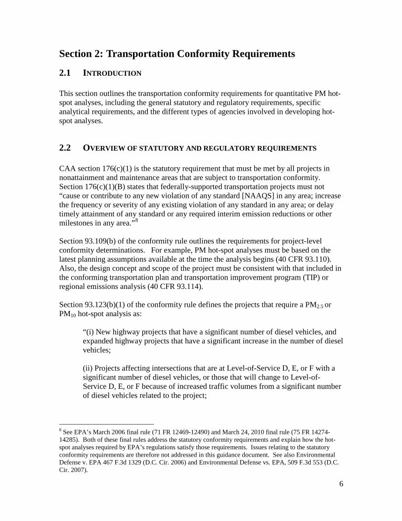
2.2 OVERVIEW OF STATUTORY AND REGULATORY REQUIREMENTS CAA section 176(c)(1) is the statutory requirement that must be met by all projects in nonattainment and maintenance areas that are subject to transportation conformity. Section 176(c)(1)(B) states that federally-supported transportation projects must not “cause or contribute to any new violation of any standard [NAAQS] in any area; increase the frequency or severity of any existing violation of any standard in any area; or delay timely attainment of any standard or any required interim emission reductions or other milestones in any area.”8

Section 93.109(b) of the conformity rule outlines the requirements for project-level conformity determinations. For example, PM hot-spot analyses must be based on the latest planning assumptions available at the time the analysis begins (40 CFR 93.110). Also, the design concept and scope of the project must be consistent with that included in the conforming transportation plan and transportation improvement program (TIP) or regional emissions analysis (40 CFR 93.114). Section 93.123(b)(1) of the conformity rule defines the projects that require a PM2.5 or PM10 hot-spot analysis as:

“(i) New highway projects that have a significant number of diesel vehicles, and expanded highway projects that have a significant increase in the number of diesel vehicles; (ii) Projects affecting intersections that are at Level-of-Service D, E, or F with a significant number of diesel vehicles, or those that will change to Level-of-Service D, E, or F because of increased traffic volumes from a significant number of diesel vehicles related to the project;

8 See EPA’s March 2006 final rule (71 FR 12469-12490) and March 24, 2010 final rule (75 FR 14274-14285). Both of these final rules address the statutory conformity requirements and explain how the hot-spot analyses required by EPA’s regulations satisfy those requirements. Issues relating to the statutory conformity requirements are therefore not addressed in this guidance document. See also Environmental Defense v. EPA 467 F.3d 1329 (D.C. Cir. 2006) and Environmental Defense vs. EPA, 509 F.3d 553 (D.C. Cir. 2007).

7

(iii) New bus and rail terminals and transfer points that have a significant number of diesel vehicles congregating at a single location; (iv) Expanded bus and rail terminals and transfer points that significantly increase the number of diesel vehicles congregating at a single location; and (v) Projects in or affecting locations, areas, or categories of sites which are identified in the PM2.5 or PM10 applicable implementation plan or implementation plan submission, as appropriate, as sites of violation or possible violation.”

A PM hot-spot analysis is not required for projects that are not of local air quality concern. For these projects, state and local project sponsors should document in their project-level conformity determinations that the requirements of the CAA and 40 CFR 93.116 are met without a hot-spot analysis, since such projects have been found not to be of local air quality concern under 40 CFR 93.123(b)(1). Note that all other project-level conformity requirements must continue to be met. See Appendix B for examples of projects that are most likely to be of local air quality concern, as well as examples of projects that are not.9

Section 93.123(c) of the conformity rule includes the general requirements for all PM hot-spot analyses. A PM hot-spot analysis must:

• Estimate the total emissions burden of direct PM emissions that may result from

the implementation of the project(s), summed together with future background concentrations;

• Include the entire transportation project, after identifying the major design features that will significantly impact local concentrations;

• Use assumptions that are consistent with those used in regional emissions analyses for inputs that are needed for both analyses (e.g., temperature, humidity);

• Assume the implementation of mitigation or control measures only where written commitments for such measures have been obtained; and

• Consider emissions increases from construction-related activities only if they occur during the construction phase and last more than five years at any individual site.

Finally, the interagency consultation process must be used to develop project-level conformity determinations to meet all applicable conformity requirements for a given project. In general, when a hot-spot analysis is required, it is done when a project-level conformity determination is completed. Conformity determinations are typically developed during the National Environmental Policy Act (NEPA) process, although conformity requirements are separate from NEPA-related requirements. There can also

9 See the preamble of the March 2006 final rule for further information regarding how and why EPA defined projects of local air quality concern (71 FR 12491-12493). EPA also clarified Section 93.123(b)(1)(i) in the January 24, 2008 final rule (73 FR 4435-4436).

8

be limited cases when conformity requirements apply after the initial NEPA process has been completed.10

2.3 INTERAGENCY CONSULTATION AND PUBLIC PARTICIPATION REQUIREMENTS

The interagency consultation process is an important tool for completing project-level conformity determinations and hot-spot analyses. Interagency consultation must be used to develop a process to evaluate and choose models and associated methods and assumptions to be used in PM hot-spot analyses (40 CFR 93.105(c)(1)(i)). For example, each area’s interagency consultation procedures must be used to determine the models and associated methods and assumptions for:

• The geographic area covered by the analysis (see Section 3.3); • The emissions models used in the analysis (see Section 4 for MOVES and

Section 5 for EMFAC); • Whether and how to estimate road and construction dust emissions (see

Section 6); • The nearby sources considered, background data used, and air quality model

chosen, including the background monitors/concentrations selected and any interpolation methods used (see Sections 7 and 8); and

• The appropriateness of receptors to be compared to the annual PM2.5 NAAQS (see Section 9.4).

State and local agencies have flexibility to decide whether the process outlined in the interagency consultation procedures should be used for aspects of PM hot-spot analyses where consultation is not required. The roles and responsibilities of various agencies for meeting the transportation conformity requirements are addressed in 40 CFR 93.105 or in a state’s approved conformity SIP. See Section 2.9 for further information on the agencies involved in interagency consultation. This guidance describes when consultation on specific decisions is necessary, but for many aspects of PM hot-spot analyses, the general requirement for interagency consultation can be satisfied without consulting separately on each and every specific decision that arises. In general, as long as the consultation requirements are met, agencies have discretion as to how they consult on hot-spot analyses. For example, the interagency consultation process could be used to make decisions on a case-by-case basis for individual transportation projects for which a PM hot-spot analysis is required. Or, agencies involved in the consultation process could develop procedures that will apply for any PM hot-spot analysis and agree that any departures from procedures would be discussed by involved agencies. For example, interagency consultation is required on the emissions model used for the analysis, but agencies could agree up front that the latest EPA-approved version of MOVES will be used for any hot-spot analysis necessary in an

10 Such an example may occur when NEPA is completed prior to an area being designated nonattainment, but additional federal project approvals are required after conformity requirements apply.

9

area that is not located in California. As a second example, agencies could agree ahead of time that, if appropriate, instead of modeling all four quarters of the year for a 24-hour PM NAAQS, only the quarters that were modeled for the latest SIP demonstration for that NAAQS need to be modeled in a hot-spot analysis. The conformity rule also requires agencies completing project-level conformity determinations to establish a proactive public involvement process that provides opportunity for public review and comment (40 CFR 93.105(e)). The NEPA public involvement process is typically used to satisfy this public participation requirement.11

If a project-level conformity determination that includes a PM hot-spot analysis is performed after NEPA is completed, a public comment period must still be provided to support that determination. In these cases, agencies have flexibility to decide what specific public participation procedures are appropriate, as long as the procedures provide a meaningful opportunity for public review and comment.

2.4 HOT-SPOT ANALYSES ARE BUILD/NO-BUILD ANALYSES

2.4.1 General As noted above, the conformity rule requires that the emissions from the proposed project, when considered with background concentrations, will not cause or contribute to any new violation, worsen existing violations, or delay timely attainment of the relevant NAAQS or required interim milestones. As described in Section 1.3, the hot-spot analysis examines the area substantially affected by the project (i.e., the “project area”). In general, a hot-spot analysis compares the air quality concentrations with the proposed project (the build scenario) to the air quality concentrations without the project (the no-build scenario).12

2.4.2 Suggested approach for PM hot-spot analyses

These air quality concentrations are determined by calculating a “design value,” a statistic that describes a future air quality concentration in the project area that can be compared to a particular NAAQS. It is always necessary to complete emissions and air quality modeling on the build scenario and compare the resulting design values to the relevant PM NAAQS. However, it will not always be necessary to conduct emissions and air quality modeling for the no-build scenario, as described further below.

To avoid unnecessary work, EPA suggests the following approach when completing a PM hot-spot analysis:

11 Section 93.105(e) of the conformity rule requires agencies to “provide opportunity for public involvement in conformity determinations for projects where otherwise required by law.” 12 See 40 CFR 93.116(a). See also November 24, 1993 conformity rule (58 FR 62212-62213). Please note that a build/no-build analysis for project-level conformity determinations is different than the build/no-build interim emissions test for regional emissions analyses in 40 CFR 93.119.

10

• First, model the build scenario and account for background concentrations in accordance with this guidance. If the design values for the build scenario are less than or equal to the relevant NAAQS, the project meets the conformity rule’s hot-spot requirements and no further modeling is needed (i.e., there is no need to model the no-build scenario). If this is not the case, the project sponsor could choose mitigation or control measures, perform additional modeling that includes these measures, and then determine if the build scenario is less than or equal to the relevant NAAQS.

• If the build scenario results in design values greater than the NAAQS, then the no-build scenario will also need to be modeled. The no-build scenario will model the air quality impacts of sources without the proposed project. The modeling results of the build and no-build scenarios should be combined with background concentrations as appropriate. If the design values for the build scenario are less than or equal to the design values for the no-build scenario, then the project meets the conformity rule’s hot-spot requirements. If not, then the project does not meet conformity requirements without further mitigation or control measures. If such measures are considered, additional modeling will need to be completed and new design values calculated to ensure that the build scenario is less than or equal to the no-build scenario.

The project sponsor can decide to use the suggested approach above or a different approach (e.g., conduct the no-build analysis first, calculate design values at all build and no-build scenario receptors). The project sponsor can choose to apply mitigation or control measures at any point in the process.13

This guidance applies to any of the above approaches for a given PM hot-spot analysis.

In general, assumptions should be consistent between the build and no-build scenarios for a given analysis year, except for traffic volumes and other project activity changes or changes in nearby sources that are expected to occur due to the project (e.g., increased activity at a nearby marine port or intermodal terminal due to a new freight corridor highway). Project sponsors should document the build/no-build analysis in the project-level conformity determination, including the assumptions, methods, and models used for each analysis year(s). The conformity rule defines how to determine if new NAAQS violations or increases in the frequency or severity of existing violations are predicted to occur based on the hot-spot analysis. Section 93.101 states: “Cause or contribute to a new violation for a project means:

(1) To cause or contribute to a new violation of a standard in the area substantially affected by the project or over a region which would

13 If mitigation or control measures are used to demonstrate conformity during the hot-spot analysis, the conformity determination for the project must include written commitments to implement such measures (40 CFR 93.125).

11

otherwise not be in violation of the standard during the future period in question, if the project were not implemented; or (2) To contribute to a new violation in a manner that would increase the frequency or severity of a new violation of a standard in such area.”

“Increase the frequency or severity means to cause a location or region to exceed

a standard more often or to cause a violation at a greater concentration than previously existed and/or would otherwise exist during the future period in question, if the project were not implemented.”

A build/no-build analysis is typically based on design value comparisons done on a receptor-by-receptor basis. However, there may be certain cases where a “new” violation at one receptor (in the build scenario) is relocated from a different receptor (in the no-build scenario). As discussed in the preamble to the November 24, 1993 transportation conformity rule, EPA believes that “a seemingly new violation may be considered to be a relocation and reduction of an existing violation only if it were in the area substantially affected by the project and if the predicted [future] design value for the “new” site would be less than the design value at the “old” site without the project – that is, if there would be a net air quality benefit” (58 FR 62213). Since 1993, EPA has made this interpretation only in limited cases with CO hot-spot analyses where there is a clear relationship between a proposed project and a possible relocated violation (e.g., a reduced CO NAAQS violation is relocated from one corner of an intersection to another due to traffic-related changes from an expanded intersection). Any potential relocated violations in PM hot-spot analyses should be determined through an area’s interagency consultation procedures.

2.4.3 Guidance focuses on refined PM hot-spot analyses Finally, the build/no-build analysis described in this guidance represents a refined PM hot-spot analysis, rather than a screening analysis. Refined analyses rely on detailed local information and simulate detailed atmospheric processes to provide more specialized and accurate estimates, and can be done for both the build and no-build scenarios. In contrast, screening analyses estimate the maximum likely air quality impacts from a given source under worst case conditions for the build scenario only.14

EPA believes that, because of the complex nature of PM emissions, the statistical form of each NAAQS, the need to consider temperature effects throughout the time period covered by the analysis, and the variability of background concentrations over the course of a year, quantitative PM hot-spot analyses need to be completed using the refined analysis procedures described in this guidance. However, there may be cases where using a screening analysis or components of a screening analysis could be supported in PM hot-spot analyses, such as: 14 Screening analyses for the 1-hour and 8-hour CO NAAQS have been completed based on peak emissions and worst case meteorology. The shorter time period covered by these NAAQS, the types of projects modeled, and other factors make screening analyses appropriate for the CO NAAQS.

12

• Where a project can be characterized as a single source (e.g., a transit terminal that could be characterized as a single area source). Such a case may be a candidate for a screening analysis using worst case travel activity and meteorological data and an appropriate screening model.15

• Where emissions modeling for a project is completed using worst case travel activity and a recommended air quality model (see Section 7.3).

Both of these options would be appropriate only for the build scenario and may be most feasible in areas where monitored PM air quality concentrations are significantly below the applicable NAAQS. In addition, other flexibilities that can simplify the hot-spot analysis process are included in later parts of this guidance (e.g., calculating design values in the build scenario first for the receptor with highest modeled concentrations only). EPA notes, however, that this guidance assumes that emissions modeling, air quality modeling, and representative background concentrations are all necessary as part of a quantitative PM hot-spot analysis in order to demonstrate conformity requirements. For example, an approach that would involve comparing only emissions between the build and no-build scenarios, without completing air quality modeling or considering representative background concentrations, would not be technically supported.16

Furthermore, EPA believes that the value of using a screening option decreases for a PM hot-spot analysis if a refined analysis will ultimately be necessary to meet conformity requirements. Evaluating and choosing models and associated methods and assumptions used in screening options must be completed through the process established by each area’s interagency consultation procedures (40 CFR 93.105(c)(1)(i)). Please consult with your EPA Regional Office, which will coordinate with EPA’s Office of Transportation and Air Quality (OTAQ) and Office of Air Quality Planning and Standards (OAQPS), if a screening analysis option is being considered for a PM hot-spot analysis.

15 Such as AERSCREEN or AERMOD using meteorological conditions suitable for screening analyses. 16 Since Section 93.123(b)(1) of the conformity rule requires PM hot-spot analyses for projects with significant new levels of PM emissions, it is unlikely that every portion of the project area in the build scenario would involve the same or fewer emissions than that same portion in the no-build scenario. Such an approach would not consider the variation of emissions and potential NAAQS impacts at different locations throughout the project area, which is necessary to meet conformity requirements.

13

2.5 EMISSIONS CONSIDERED IN PM HOT-SPOT ANALYSES

2.5.1 General requirements PM hot-spot analyses include only directly emitted PM2.5 or PM10 emissions. PM2.5 and PM10 precursors are not considered in PM hot-spot analyses, since precursors take time at the regional level to form into secondary PM.17

2.5.2 PM emissions from motor vehicle exhaust, brake wear, and tire wear

Exhaust, brake wear, and tire wear emissions from on-road vehicles are always be included in a project’s PM2.5 or PM10 hot-spot analysis. See Sections 4 and 5 for how to quantify these emissions using MOVES (outside California) or EMFAC (within California).

2.5.3 PM2.5 emissions from re-entrained road dust Re-entrained road dust must be considered in PM2.5 hot-spot analyses only if EPA or the state air agency has made a finding that such emissions are a significant contributor to the PM2.5 air quality problem in a given nonattainment or maintenance area (40 CFR 93.102(b)(3) and 93.119(f)(8)).18

• If a PM2.5 area has no adequate or approved SIP budgets for the PM2.5 NAAQS, re-entrained road dust is not included in a hot-spot analysis unless the EPA Regional Administrator or state air quality agency determines that re-entrained road dust is a significant contributor to the PM2.5 nonattainment problem and has so notified the metropolitan planning organization (MPO) and DOT.

• If a PM2.5 area has adequate or approved SIP budgets, re-entrained road dust

would have to be included in a hot-spot analysis only if such budgets include re-entrained road dust.

See Section 6 for further information regarding how to estimate re-entrained road dust for PM2.5 hot-spot analyses, if necessary.

2.5.4 PM10 emissions from re-entrained road dust Re-entrained road dust must be included in all PM10 hot-spot analyses. Because road dust is a significant component of PM10 inventories, EPA has historically required road dust emissions to be included in all conformity analyses of direct PM10 emissions –

17 See 40 CFR 93.102(b) for the general requirements for applicable pollutants and precursors in conformity determinations. Section 93.123(c) provides additional information regarding certain PM emissions for hot-spot analyses. See also EPA’s March 2006 final rule preamble (71 FR 12496-8). 18 See the July 1, 2004 final conformity rule (69 FR 40004).

14

including hot-spot analyses.19

2.5.5 PM emissions from construction-related activities

See Section 6 for further information regarding how to estimate re-entrained road dust for PM10 hot-spot analyses.

Emissions from construction-related activities are not required to be included in PM hot-spot analyses if such emissions are considered temporary as defined in 40 CFR 93.123(c)(5) (i.e., emissions which occur only during the construction phase and last five years or less at any individual site). Construction emissions would include any direct PM emissions from construction-related dust and exhaust emissions from construction vehicles and equipment. For most projects, construction emissions would not be included in PM2.5 or PM10 hot-spot analyses (because, in most cases, the construction phase is less than five years at any one site).20

However, there may be limited cases where a large project is constructed over a longer time period, and non-temporary construction emissions must be included when an analysis year is chosen during project construction. See Section 6 for further information regarding how to estimate transportation-related construction emissions for PM hot-spot analyses, if necessary.

2.6 NAAQS CONSIDERED IN PM HOT-SPOT ANALYSES The CAA and transportation conformity regulations require that conformity be met for all transportation-related NAAQS for which an area has been designated nonattainment or maintenance. Therefore, a project-level conformity determination must address all applicable NAAQS for a given pollutant.21

Accordingly, results from a quantitative hot-spot analysis will need to be compared to all relevant PM2.5 and PM10 NAAQS in effect for the area undertaking the analysis. For example, in an area designated nonattainment or maintenance for only the annual PM2.5 NAAQS or only the 24-hour PM2.5 NAAQS, the hot-spot analysis would have to address only that respective PM2.5 NAAQS. If an area is designated nonattainment or maintenance for the annual and 24-hour PM2.5 NAAQS, the hot-spot analysis would have to address both NAAQS for conformity purposes.

2.7 BACKGROUND CONCENTRATIONS As required by 40 CFR 93.123(c)(1) and discussed in Section 2.2, a PM hot-spot analysis “must be based on the total emissions burden which may result from the implementation of the project, summed together with future background concentrations….” By 19 See the March 2006 final rule (71 FR 12496-98). 20 EPA’s rationale for limiting the consideration of construction emissions to five years can be found in its January 11, 1993 proposed rule (58 FR 3780). 21 See EPA’s March 2006 final rule (71 FR 12468-12511).

15

definition, background concentrations do not include emissions from the project itself. Background concentrations include the emission impacts of all sources that affect concentrations in the project area other than the project. Section 8 provides further information on how background concentrations can be determined.

2.8 APPROPRIATE TIME FRAME AND ANALYSIS YEARS Section 93.116(a) of the conformity rule requires that PM hot-spot analyses consider either the full time frame of an area's transportation plan or, in an isolated rural nonattainment or maintenance area, the 20-year regional emissions analysis.22

Conformity requirements are met if the analysis demonstrates that no new or worsened violations occur in the year(s) of highest expected emissions – which includes the project’s emissions in addition to background concentrations.23

• Peak emissions from the project are expected; and

Areas should analyze the year(s) within the transportation plan or regional emissions analysis, as appropriate, during which:

• A new NAAQS violation or worsening of an existing violation would most likely occur due to the cumulative impacts of the project and background concentrations in the project area.

If such a demonstration occurs, then no adverse impacts would be expected to occur in any other years within the time frame of the transportation plan or regional emissions analysis.24

The following factors (among others) should be considered when selecting the year(s) of peak emissions:

• Changes in vehicle fleets; • Changes in traffic volumes, speeds, and vehicle miles traveled (VMT); and • Expected trends in background concentrations, including any nearby sources that

are affected by the project. In some cases, selecting only one analysis year, such as the last year of the transportation plan or the year of project completion, may not be sufficient to satisfy conformity requirements. For example, if a project is being developed in two stages and the entire two-stage project is being approved, two analysis years should be modeled: one to examine the impacts of the first stage of the project and another to examine the impacts

22 Although CAA section 176(c)(7) and 40 CFR 93.106(d) allow the election of changes to the time horizons for transportation plan and TIP conformity determinations, these changes to do not affect the time frame and analysis requirements for hot-spot analyses. 23 If such a demonstration can be made, then EPA believes it is reasonable to assume that no adverse impacts would occur in any other years within the time frame of the transportation plan or regional emissions analysis. 24 See EPA’s July 1, 2004 final conformity rule (69 FR 40056-40058).

16

of the completed project.25

Selecting appropriate analysis year(s) should be considered through the process established by each area’s interagency consultation procedures (40 CFR 93.105(c)(1)(i)).

2.9 AGENCY ROLES AND RESPONSIBILITIES The typical roles and responsibilities of agencies implementing the PM hot-spot analysis requirements are described below. Further details are provided throughout later sections of this guidance.

2.9.1 Project sponsor The project sponsor is typically the agency responsible for implementing the project (e.g., a state department of transportation, regional or local transit operator, or local government). The project sponsor is the lead agency for developing the PM hot-spot analysis, meeting interagency consultation and public participation requirements, and documenting the final hot-spot analysis in the project-level conformity determination.

2.9.2 DOT DOT is responsible for making project-level conformity determinations. PM hot-spot analyses and conformity determinations would generally be included in documents prepared to meet NEPA requirements. It is possible for DOT to make a project-level conformity determination outside of the NEPA process (for example, if conformity requirements apply after NEPA has been completed, but additional federal action on the project is required). DOT is also an active member of the interagency consultation process for conformity determinations.

2.9.3 EPA EPA is responsible for promulgating transportation conformity regulations and provides policy and technical assistance to federal, state, and local conformity implementers. EPA is an active member of the interagency consultation process for conformity determinations. In addition, EPA reviews submitted SIPs, and provides policy and technical support for emissions modeling, air quality modeling, monitoring, and other issues.

2.9.4 State and local transportation and air agencies State and local transportation and air quality agencies are part of the interagency consultation process and assist in modeling of transportation activities, emissions, and air quality. These agencies are likely to provide data required to perform a PM hot-spot analysis, although the conformity rule does not specifically define the involvement of

25 See EPA’s July 1, 2004 final rule (69 FR 40057).

17

these agencies in project-level conformity determinations. For example, the state or local air quality agency operates the air quality monitoring network, processes meteorological data, and uses air quality models for air quality planning purposes (such as SIP development and modeling applications for other purposes). MPOs often conduct emissions modeling, maintain regional population forecasts, and estimate future traffic conditions relevant for project planning. The interagency consultation process can be used to discuss the role of the state or local air agency, the MPO, and other agencies in project-level conformity determinations, if such roles are not already defined in an area’s conformity SIP.

18

Section 3: Overview of a Quantitative PM Hot-Spot Analysis

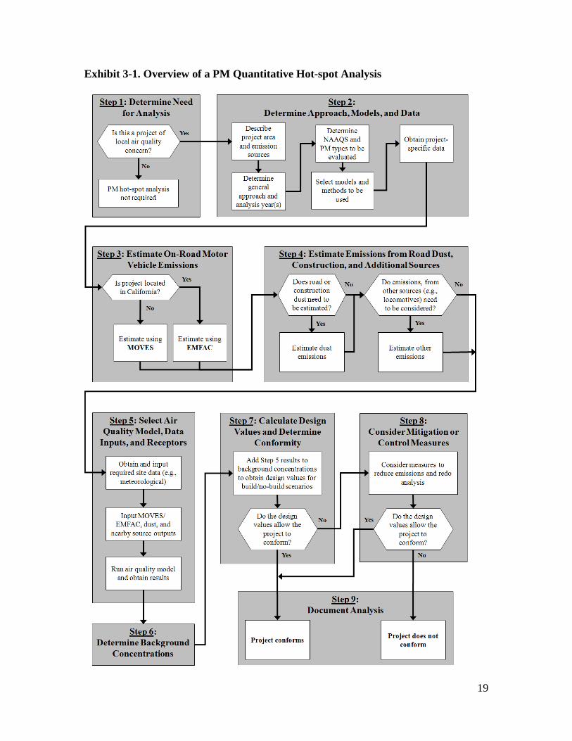
3.1 INTRODUCTION This section provides a general overview of the process for conducting a quantitative PM hot-spot analysis. All individual elements or steps presented here are covered in more depth and with more technical information throughout the remainder of the guidance. The general steps required to complete a quantitative PM hot-spot analysis are depicted in Exhibit 3-1 (following page) and summarized in this section. As previously noted in Section 2.3, the interagency consultation process is an essential part of developing PM hot-spot analyses. As a number of fundamental aspects of the analysis need to be determined through consultation, it is recommended that these discussions take place as early and as often as necessary for the analysis to be completed on schedule. In addition, early consultation allows potential data sources for the analysis to be more easily identified.

3.2 DETERMINE NEED FOR A PM HOT-SPOT ANALYSIS (STEP 1) The conformity rule requires a PM hot-spot analysis only for projects of local air quality concern. See Section 2.2 regarding how to determine if a project is of local air quality concern according to the conformity rule. 3.3 DETERMINE APPROACH, MODELS, AND DATA (STEP 2)

3.3.1 General There are several decisions that need to be made before beginning a PM hot-spot analysis, including determining the:

• Geographic area to be covered by the analysis (the “project area”) and emission sources to be modeled;

• General approach and analysis year(s) for emissions and air quality modeling; • Applicable PM NAAQS to be evaluated; • Type of PM emissions to be modeled for different sources; • Emissions and air quality models and methods to be used; • Project-specific data to be used; and • Schedule for conducting the analysis and points of consultation.

Further details on these decisions are provided below. Evaluating and choosing models and associated methods and assumptions must be completed through the process established by each area’s interagency consultation procedures (40 CFR 93.105(c)(1)(i)).

19

Exhibit 3-1. Overview of a PM Quantitative Hot-spot Analysis

20

3.3.2 Determining the geographic area and emission sources to be covered by the analysis

The geographic area to be covered by a PM hot-spot analysis (the “project area”) is to be determined on a case-by-case basis.26 PM hot-spot analyses must examine the air quality impacts for the relevant PM NAAQS in the area substantially affected by the project (40 CFR 93.123(c)(1)). To meet this and other conformity requirements, it is necessary to define the project, determine where it is to be located, and ascertain what other emission sources are located in the project area.27 In addition to emissions from the proposed highway or transit project,28

there may be nearby sources of emissions that need to be estimated and included in air quality modeling (e.g., a freight rail terminal that is affected by the project). There also may be other sources in the project area that are determined to be insignificant to project emissions (e.g., a service drive or small employee parking lot). See Sections 4 through 6 for how to estimate emissions from the proposed project, and Sections 6 through 8 for when and how to include nearby source emissions and other background concentrations.

Hot-spot analyses must include the entire project (40 CFR 93.123(c)(2)). However, it may be appropriate in some cases to focus the PM hot-spot analysis only on the locations of highest air quality concentrations. For large projects, it may be necessary to analyze multiple locations that are expected to have the highest air quality concentrations and, consequently, the most likely new or worsened PM NAAQS violations. If conformity is demonstrated at such locations, then it can be assumed that conformity is met in the entire project area. For example, if a highway project involves several lane miles with similar travel activity (and no nearby sources that need to be modeled), the scope of the PM hot-spot analysis could involve only the point(s) of highest expected PM concentrations. If conformity requirements are met at such locations, then it can be assumed that conformity is met throughout the project area. Such an approach would be preferable to modeling the entire length of the highway project, which would involve additional time and resources. Questions regarding the scope of a given PM hot-spot analysis can be determined through the interagency consultation process.

3.3.3 Deciding the general analysis approach and analysis year(s) As stated in Section 2.4, there are several approaches for completing a build/no-build analysis for a given project. For example, a project sponsor may want to start by completing the build scenario first to see if a new or worsened PM NAAQS violation is

26 Given the variety of potential projects that may require a PM hot-spot analysis, it is not possible to provide one definition or set of parameters that can be used in all cases to determine the area covered by the PM hot-spot analysis. 27 See more in the March 24, 2010 final conformity rule entitled “Transportation Conformity Rule PM2.5 and PM10 amendments,” 75 FR 14281; found online at: www.epa.gov/otaq/stateresources/transconf/conf-regs.htm. 28 40 CFR 93.101 defines “highway project” and “transit project” for transportation conformity purposes.

http://www.epa.gov/otaq/stateresources/transconf/conf-regs.htm�

http://www.epa.gov/otaq/stateresources/transconf/conf-regs.htm�

21

predicted (if not, then modeling the no-build scenario would be unnecessary). In contrast, a project sponsor could start with the no-build scenario first if a future PM NAAQS violation is anticipated in both the build and no-build scenarios (even after mitigation or control measures are considered). It is also necessary to select one or more analysis years within the time frame of the transportation plan or regional emissions analysis when emissions from the project, any nearby sources, and background are expected to be highest. See Section 2.8 for more information on selecting analysis year(s).

3.3.4 Determining the PM NAAQS to be evaluated As stated in Section 2.6, PM hot-spot analyses need to be evaluated only for the NAAQS for which an area has been designated nonattainment or maintenance. In addition, there are aspects of modeling that can be affected by whether a NAAQS is an annual or a 24-hour PM NAAQS. It is also important to conduct modeling for those parts of an analysis year where PM concentrations are expected to be highest. For example, a hot-spot analysis for the annual PM2.5 NAAQS would involve data and modeling throughout a given analysis year (i.e., all four quarters of the analysis year).29

A hot-spot analysis for the 24-hour PM2.5 or PM10 NAAQS would also involve data and modeling throughout an analysis year, except when future NAAQS violations and peak emissions in the project area are expected to occur in only one quarter of the future analysis year(s). In such cases, a project sponsor could choose to complete emissions and air quality modeling for only that quarter, as determined through the interagency consultation process. For example, if an area’s SIP demonstration is based on only one quarter for a 24-hour PM NAAQS, it may be appropriate to make the same assumption for hot-spot analyses for that NAAQS. This could be the case in a PM10 nonattainment or maintenance area that has PM10 NAAQS violations only during the first quarter of the year (January-March), when PM emissions from other sources, such as wood smoke, are highest. In such an area, if the highest emissions from the project area are also expected to occur in this same quarter, then the project sponsor could complete the PM hot-spot analysis for only that quarter. EPA notes, however, that it may be difficult to determine whether 24-hour PM2.5 NAAQS violations will occur in only one quarter. State and local air quality agencies should be consulted regarding when it may be appropriate for a PM hot-spot analysis for a 24-hour PM NAAQS to cover only one quarter in an analysis year. These agencies are responsible for monitoring air quality violations and for developing SIP attainment demonstrations.

29 Calendar quarters in this guidance are defined in the following manner: Q1 (January-March), Q2 (April-June), Q3 (July-September), and Q4 (October-December). These quarters are also used by EPA and state and local agencies to calculate design values for air quality monitoring purposes and for SIP development.

22

3.3.5 Deciding on the type of PM emissions to be modeled See Section 2.5 for further information on what types of directly emitted PM must be included in hot-spot analyses and Sections 4 through 6 and Section 8 on when and how to quantify PM emissions.

3.3.6 Determining the models and methods to be used The emissions and air quality models and methods used in PM hot-spot analyses must be evaluated and chosen through the process established by each area’s interagency consultation procedures (40 CFR 93.105(c)(1)(i)). The latest approved emissions models must be used in PM hot-spot analyses (40 CFR 93.111). See Sections 3.4 through 3.6 and the subsequent sections of the guidance they refer to for specific information about models and methods that apply. Note: It is important to select an air quality model to be used in the PM hot-spot analysis early in the process, since this information is necessary to prepare emissions model outputs for air quality modeling purposes. See Section 7 for further information on when AERMOD and CAL3QHCR are recommended air quality models for PM hot-spot analyses.

3.3.7 Obtaining project-specific data The conformity rule requires that the latest planning assumptions available at the time that the analysis begins be used in conformity determinations (40 CFR 93.110). In addition, the regulation states that hot-spot analysis assumptions must be consistent with those assumptions used in the regional emissions analysis for any inputs that are required for both analyses (40 CFR 93.123(c)(3)). The project sponsor should use project-specific data for both emissions and air quality modeling whenever possible, though default inputs may be appropriate in some cases. The use of project-specific versus default data is discussed further in this guidance. The following are examples of data needed to run MOVES or EMFAC, as described in Sections 4 and 5:

• Traffic data sufficient to characterize each link in the project area; • Starts per hour and number of vehicles idling during each hour for off-network

links/sources; • Vehicle types and age distribution expected in the project area; and • Temperature and humidity data for each month and hour included in the analysis.

Depending on the air quality model to be used, the following are examples of data that will likely be needed, as described in Sections 7 through 9:

• Surface meteorological data from monitors that measure the atmosphere near the ground;

23

• Upper air data describing the vertical temperature profile of the atmosphere; • Land use data describing surface characteristics near the surface meteorological

monitors; • Nearby population data; and • Information necessary for determining locations of air quality modeling receptors.

To complete the PM hot-spot analysis, areas will also need data on background concentrations in the project area from nearby or other emission sources, as described in Section 8.

3.4 ESTIMATE ON-ROAD MOTOR VEHICLE EMISSIONS (STEP 3) There are two approved motor vehicle emissions models available for estimating the project’s exhaust, brake wear, and tire wear emissions. See Section 4 for more on estimating these PM emissions with EPA’s MOVES model. Section 5 describes how to apply EMFAC for estimating these emissions for projects in California.

3.5 ESTIMATE EMISSIONS FROM ROAD DUST, CONSTRUCTION, AND ADDITIONAL SOURCES (STEP 4)

Section 2.5 provides more information about when re-entrained road dust and/or construction emissions are included in PM hot-spot analyses. Section 6 describes methods for estimating these emissions. There may be other sources of emissions that also need to be estimated, and included in air quality modeling. Section 8 provides further information regarding how to account for these emissions in a PM hot-spot analysis and Appendix I describes how to estimate locomotive emissions.

3.6 SELECT AN AIR QUALITY MODEL, DATA INPUTS AND RECEPTORS (STEP 5)

An air quality model estimates PM concentrations at specific points in the project area known as “receptors.” Emissions that result from the project (including those from vehicles, dust, and construction from Steps 3 and 4) as well as any other nearby emission sources that are affected by the project (e.g., expanded locomotive emissions at a freight terminal) are included in the selected air quality model, which predicts how emissions are dispersed based on meteorological and other input data. There are two air quality models—AERMOD and CAL3QHCR— recommended for use in PM hot-spot analyses, depending on the project involved. Basic information about

24

these models, including how to select an appropriate model for a particular project and the data needed to run them, is found in Section 7 and Appendix J.

3.7 DETERMINE BACKGROUND CONCENTRATIONS FROM NEARBY AND OTHER SOURCES (STEP 6)

The PM hot-spot analysis must also account for background PM concentrations in the project area. Section 8 provides further information on selecting representative background concentrations, including when to incorporate nearby sources into air quality modeling.

3.8 CALCULATE DESIGN VALUES AND DETERMINE CONFORMITY (STEP 7) In general, the PM concentrations estimated from air quality modeling (from Step 5) are then combined with background concentrations (from Step 6) at the receptor locations for both the build and no-build scenarios. The resulting statistic is referred to as a design value; how it is calculated depends on the form of the NAAQS. If the design value in the build scenario is less than or equal to the relevant PM NAAQS at appropriate receptors, then the project meets conformity requirements. In the case where the design value is greater than the NAAQS in the build scenario, a project could still meet conformity requirements if the design values in the build scenario were less than or equal to the design values in the no-build scenario at appropriate receptors. See Sections 2.4 and 9 for further details on build/no-build approaches and implementation.

25

3.9 CONSIDER MITIGATION OR CONTROL MEASURES (STEP 8) Where a project does not meet conformity requirements, a project sponsor may consider mitigation or control measures to reduce emissions in the project area. If such measures are considered, additional modeling will need to be completed and new design values calculated to ensure that conformity requirements are met. A project sponsor could decide to add mitigation or control measures at any time in the process; such measures must include written commitments for implementation (40 CFR 93.125). See Section 10 for more information on possible measures for consideration.

3.10 DOCUMENT THE PM HOT-SPOT ANALYSIS (STEP 9) The PM hot-spot analysis should include sufficient documentation to support the conclusion that a proposed project meets conformity rule requirements per 40 CFR 93.116 and 93.123. This documentation should include, at a minimum:

• A description of the proposed project, including where the project is located, the project’s scope (e.g., adding an interchange, widening a highway, expanding a major bus terminal), when the project is expected to be open to traffic, travel activity projected for the analysis year(s), and what part of 40 CFR 93.123(b)(1) applies;30

• A description of the analysis year(s) examined and the factors considered in determining the year(s) of peak emissions;

• Emissions modeling, including the emissions model used (e.g., MOVES), modeling inputs and results, and how the project was characterized in terms of links;

• Modeling inputs and results for estimating re-entrained road dust, construction emissions, and any nearby source emissions (if applicable to a particular PM hot-spot analysis);

• Air quality modeling data, including the air quality model used, modeling inputs and results, and description of the receptors employed in the analysis;

• A description of the assumptions used to determine background concentrations; • A discussion of any mitigation or control measures that will be implemented, the

methods and assumptions used to quantify their expected effects, and associated written commitments;

• A description of how the interagency consultation and public participation requirements in 40 CFR 93.105 were met; and

• A conclusion for how the proposed project meets 40 CFR 93.116 and 93.123 conformity requirements for the PM2.5 and/or PM10 NAAQS.

Documentation should describe the sources of data used in preparing emissions and air quality modeling inputs. This documentation should also describe any critical 30 This information could reference the appropriate sections of any NEPA document prepared for the project.

26

assumptions that have the potential to affect predicted concentrations. Documentation of PM hot-spot analyses would be included in the project-level conformity determination.

27

Section 4: Estimating Project-Level PM Emissions Using MOVES

4.1 INTRODUCTION This section of the guidance describes how to use MOVES to estimate PM exhaust, brake wear, and tire wear emissions for PM hot-spot analyses outside of California.31 This section focuses on determining the appropriate project-level inputs and how MOVES should be run to provide the necessary information to complete air quality modeling.32

MOVES is a computer model designed by EPA to estimate emissions from cars, trucks, buses and motorcycles. MOVES replaces MOBILE6.2, EPA’s previous emissions model.33

MOVES is based on an extensive review of in-use vehicle data collected and analyzed since the release of MOBILE6.2. MOVES estimates PM emissions to account for speed and temperature variations and models emissions at a high resolution. As a result, MOVES allows users to incorporate a much wider array of vehicle activity data for each roadway link, as well as start and extended idle activity in transit or other terminal projects.

Exhibit 4-1 (following page) shows the necessary steps for applying the MOVES model for project-level PM hot-spot analyses. This section presumes users already have a basic understanding of how to run the MOVES model.34

MOVES includes a default database of meteorology, fleet, activity, fuel, and control program data for the entire United States. The data included in this database come from a variety of sources which are not necessarily the most accurate or up-to-date information available at the local level for a particular project. This section describes when the use of that default database is appropriate for PM hot-spot analysis, as well as when available local data must be used (40 CFR 93.110 and 93.123(c)).

31 This guidance is applicable to current and future versions of the MOVES model, unless EPA notes otherwise when approving the model for conformity purposes. 32 Technical guidance on using MOVES for regional emissions inventories can be found in “Technical Guidance on the Use of MOVES2010 for Emission Inventory Preparation in State Implementation Plans and Transportation Conformity,” EPA-420-B-10-023 (April 2010); available online at: www.epa.gov/otaq/stateresources/transconf/policy.htm. 33 EPA stated in the preamble to the March 2006 final rule that finalizing the MOVES emissions model was critical before quantitative PM hot-spot analyses are required, due to the limitations of applying MOBILE6.2 for PM at the project level. See EPA’s March 2006 final rule for further information (71 FR 12498-12502). 34 The MOVES model, user guide, and supporting documentation are available online at: www.epa.gov/otaq/models/moves/index.htm.


http://www.epa.gov/otaq/models/moves/index.htm�

28

Exhibit 4-1. Steps for Using MOVES in a Quantitative PM Hot-spot Analysis

Note: The steps in this exhibit and in the accompanying text describe how to use MOVES at the project-level for a PM hot-spot analysis.

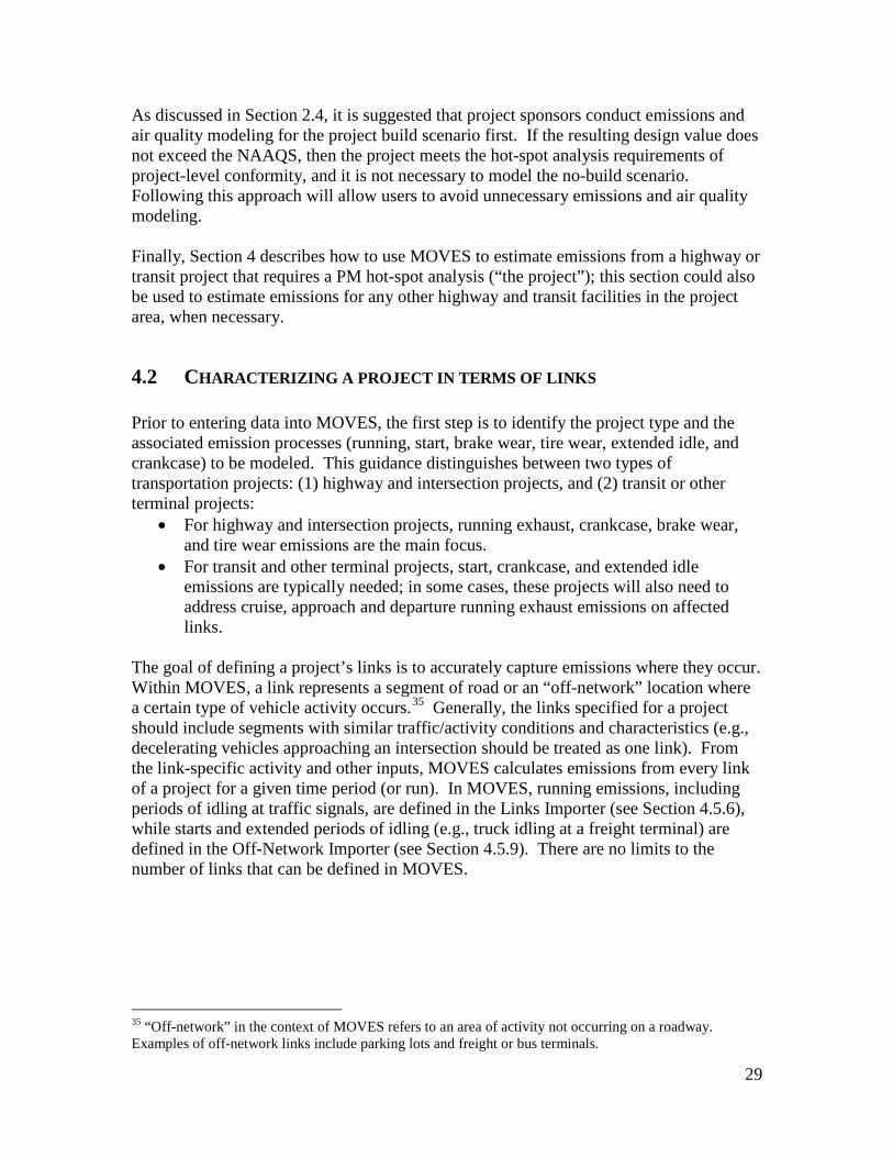
29

As discussed in Section 2.4, it is suggested that project sponsors conduct emissions and air quality modeling for the project build scenario first. If the resulting design value does not exceed the NAAQS, then the project meets the hot-spot analysis requirements of project-level conformity, and it is not necessary to model the no-build scenario. Following this approach will allow users to avoid unnecessary emissions and air quality modeling. Finally, Section 4 describes how to use MOVES to estimate emissions from a highway or transit project that requires a PM hot-spot analysis (“the project”); this section could also be used to estimate emissions for any other highway and transit facilities in the project area, when necessary.

4.2 CHARACTERIZING A PROJECT IN TERMS OF LINKS Prior to entering data into MOVES, the first step is to identify the project type and the associated emission processes (running, start, brake wear, tire wear, extended idle, and crankcase) to be modeled. This guidance distinguishes between two types of transportation projects: (1) highway and intersection projects, and (2) transit or other terminal projects:

• For highway and intersection projects, running exhaust, crankcase, brake wear, and tire wear emissions are the main focus.

• For transit and other terminal projects, start, crankcase, and extended idle emissions are typically needed; in some cases, these projects will also need to address cruise, approach and departure running exhaust emissions on affected links.

The goal of defining a project’s links is to accurately capture emissions where they occur. Within MOVES, a link represents a segment of road or an “off-network” location where a certain type of vehicle activity occurs.35

35 “Off-network” in the context of MOVES refers to an area of activity not occurring on a roadway. Examples of off-network links include parking lots and freight or bus terminals.

Generally, the links specified for a project should include segments with similar traffic/activity conditions and characteristics (e.g., decelerating vehicles approaching an intersection should be treated as one link). From the link-specific activity and other inputs, MOVES calculates emissions from every link of a project for a given time period (or run). In MOVES, running emissions, including periods of idling at traffic signals, are defined in the Links Importer (see Section 4.5.6), while starts and extended periods of idling (e.g., truck idling at a freight terminal) are defined in the Off-Network Importer (see Section 4.5.9). There are no limits to the number of links that can be defined in MOVES.

30

4.2.1 Highway and intersection projects General A PM hot-spot analysis fundamentally depends on the availability of accurate data on roadway link speed and traffic volumes for build and no-build scenarios.36

Thus, local traffic data should be used to characterize each link sufficiently. It is recommended that the user divide a project into separate links to allow sufficient resolution at different vehicle traffic and activity patterns; characterizing this variability in emissions within the project area will assist in air quality modeling (see Section 7).

In MOVES, activity on free-flow highway links can be defined by an average speed, link drive schedule, or operating mode (“Op-Mode”) distribution (discussed in Section 4.5.7). For analyses with MOVES, average speed and traffic volume, at a minimum, is needed for each link. If no other information is available, MOVES uses default assumptions of vehicle activity patterns (called drive cycles) for average speed and type of roadway to estimate emissions. Default drive cycles use different combinations of vehicle activity (acceleration, deceleration, cruise, and/or idle) depending on the speed and road type. For example, if the link average speed is 30 mph and it is an urban arterial (urban unrestricted road type), MOVES uses a default drive cycle that includes a high proportion of acceleration, deceleration, and idle activity as would be expected on an urban arterial with frequent stops. If the average speed is 60 mph and it is a rural freeway (rural restricted road type), MOVES uses a default drive cycle that assumes a higher proportion of cruise activity, smaller proportions of acceleration and deceleration activity, and little or no idle activity. Project sponsors should determine average congested speeds by using appropriate methods based on best practices used for highway analysis.37 Some resources are available through FHWA’s Travel Model Improvement Program (TMIP).38 Methodologies for computing intersection control delay are provided in the Highway Capacity Manual 2000.39

As described further in Section 4.5.7, users should take advantage of the full capabilities of MOVES for estimating emissions on different highway and intersection project links.

36 Project sponsors should document available traffic data sets, their sources, key assumptions, and the methods used to develop build and no-build scenario inputs for MOVES. Documentation should include differences between how build and no-build traffic projections are obtained. For projects of local air quality concern, differences in traffic volumes and other activity changes between the build and no-build scenarios must be accounted for in the data that is used in the PM hot-spot analysis. 37 As discussed in Section 7, the use of the CAL3QHCR queuing algorithm for intersection idle queues is not recommended. Rather, idling vehicles should be represented in combination with decelerating, accelerating, and free-flow traffic on an approach segment of an intersection. 38 See FHWA’s TMIP website: http://tmip.fhwa.dot.gov/. 39 Users should consult the most recent version of the Highway Capacity Manual. As of the release of this guidance, the latest version is the Highway Capacity Manual 2000, which can be obtained from the Transportation Research Board (see http://144.171.11.107/Main/Public/Blurbs/152169.aspx for details).

http://tmip.fhwa.dot.gov/�

http://144.171.11.107/Main/Public/Blurbs/152169.aspx�

31

Although average speeds and travel volumes are typically available for most transportation projects and may need to be relied upon during the transition to using MOVES, users can develop and use more precise data through the MOVES Operating Mode Distribution Importer or Link Drive Schedule Importer, as described further below. When more detailed data are available to describe the pattern of changes in vehicle activity (proportion of time in acceleration, deceleration, cruise, or idle activity) over a length of road, MOVES is capable of calculating these specific emission impacts. EPA encourages users to consider these options for highway and intersection projects, especially as MOVES is implemented further into the future, or for more advanced MOVES applications. Free-flow Highway Links The links defined in MOVES should capture the expected physical layout of a project and representative variations in vehicle activity. A simple example would be a single, one directional, four-lane highway that could be characterized as just one link. More sophisticated analyses may break up traffic flow on that single link into multiple links of varying operating modes or drive cycles that may have different emission factors depending on the relative acceleration, cruise, or deceleration activity on each segment of that link. In general, the definition of a link will depend on how much the type of vehicle activity (acceleration, deceleration, cruise or idle) changes over a length of roadway, the level of detail of available data, and the modeling approach used with MOVES. For a highway lane where vehicle behavior is fairly constant, the length of the link could be longer and the use of detailed activity data will have a smaller impact on results. Intersection Links If the project analysis involves intersections, the intersections need to be treated separately from the free-flow links that connect to those intersections. Although road segments between intersections may experience free-flow traffic operations, the approaches and departures from the intersections will likely involve acceleration, deceleration, and idling activity not present on the free-flow link. For intersection modeling, the definition of link length will depend on the geometry of the intersection, how that geometry affects vehicle activity, and the level of detail of available activity information. Guidance for defining intersection links is given in Appendix D, but the definition of links used for a particular project will depend of the specific details of that project and the amount of available activity information.40

Note: For both free-flow highway and intersection links, users may directly enter output from traffic simulation models in the form of second-by-second individual vehicle trajectories. These vehicle trajectories for each road segment can be input into MOVES using the Link Drive Schedule Importer and defined as unique LinkIDs. There are no limits in MOVES as to how many links can be defined; however, model run times

40 As discussed in Section 7, the use of the CAL3QHCR queuing algorithm for intersection idle queues is not recommended. Rather, idling vehicles should be represented in combination with decelerating, accelerating, and free-flow traffic on an approach segment of an intersection.

32

increase as the user defines more links. More information on using vehicle trajectories from traffic micro-simulation models is found in Appendix D.

4.2.2 Transit and other terminal projects For off-network sources such as a bus terminal or intermodal freight terminal, the user should have information on starts per hour and number of vehicles idling during each hour. This activity will likely vary from hour to hour. Additionally, if there are vehicles starting, it is necessary to provide an estimate of the duration that vehicles are parked before starting (soak-time distribution). It is recommended that the user divide such a project into separate links to appropriately characterize variability in emission density within the project area (as discussed in Section 7). In this case, each “link” describes an area with a certain number of vehicle starts per hour, or a certain number of vehicles idling during each hour. Some transit and other terminal projects may have significant running emissions similar to free-flow highway projects (such as buses and trucks coming to and from an intermodal terminal). These emissions can be calculated by defining one or more unique running links as described in Section 4.2.1 and Appendix D (that is, in addition to any other roadway links associated with the project). These running link emissions can then be aggregated with the emissions from starts and idling from non-running activity on the transit or other terminal link outside of the MOVES model to generate the necessary air quality model inputs. Long duration idling (classified in MOVES as OpModeID 200) can only be modeled in MOVES for long-haul combination trucks. Idling for other vehicles and shorter periods of idling for long-haul combination trucks should be modeled as a project link with an operating mode distribution that consists only of idle operation (OpMode 1). This can be specified in the Links table by inputting the vehicle population and specifying an average speed of “0” mph. Note: The user may choose to exclude sources such as a separate service drive, separate small employee parking lot, or other minor sources that are determined to be insignificant to project emissions.

4.3 DETERMINING THE NUMBER OF MOVES RUNS

4.3.1 General When MOVES is run at the project scale, it estimates emissions for only the hour specified by the user. Before running MOVES to calculate emission factors, users should first determine the number of unique scenarios that can sufficiently describe activity variation in a project. In most projects, traffic volume, average speed, idling, fleet mix, and the corresponding emission factors will likely vary from hour to hour, day to day, and month to month. However, it is unlikely that data are readily available that capture

33

such finite changes. Project sponsors may have activity data collected at a range of possible temporal resolutions. The conformity rule requires the use of the latest planning assumptions or data available at the time the conformity analysis begins (40 CFR 93.110).41

Depending on the sophistication of the activity data analysis for a given project, these data may range from a daily average-hour and peak-hour value to hourly estimates for all days of the year. EPA encourages the development of sufficient travel activity data to capture the expected ranges of traffic conditions for the build and no-build scenarios.

The number of MOVES runs should be based on the best available activity data and the PM NAAQS involved. One of the advantages to using MOVES is that, for the first time, PM emission estimates are sensitive to temperature changes through a day and across a year. Therefore, EPA is recommending the minimum number of MOVES runs that is necessary for PM hot-spot analysis to capture changes in emission rates due to changes in ambient conditions.42

Exhibit 4-2 includes EPA’s recommendations for PM hot-spot analyses:

Exhibit 4-2. Typical Number of MOVES Runs for an Analysis Year Applicable NAAQS Build Scenario No-build Scenario43 Annual PM2.5 NAAQS only 16 16 24-hour PM2.5 NAAQS only 16 (4 in certain cases) 16 (4 in certain cases) 24-hour PM10 NAAQS only 16 (4 in certain cases) 16 (4 in certain cases) Annual and 24-hour PM NAAQS44 16 16

Hot-spot analyses for the annual PM2.5 NAAQS should include 16 unique MOVES runs (i.e., four runs for different time periods for each of four calendar quarters). For a typical build/no-build analysis, a total of 32 runs would be needed (16 for the build scenario and 16 for the no-build scenario). Hot-spot analyses for only the 24-hour PM2.5 or PM10 NAAQS should also be completed with 16 MOVES runs for each scenario, except in cases where potential PM NAAQS violations are expected to occur in only one quarter of the calendar year. In such cases, the user may choose to model only that quarter with

41 See “EPA and DOT Joint Guidance for the Use of Latest Planning Assumptions in Transportation Conformity Determinations,” EPA-420-B-08-901 (December 2008) for a more detailed discussion of the latest planning assumptions requirements: www.epa.gov/otaq/stateresources/transconf/policy/420b08901.pdf. 42 Information on PM emission rate sensitivity to temperature inputs is available in “Draft MOVES2009 Highway Vehicle Temperature, Humidity, Air Conditioning, and Inspection and Maintenance Adjustments” at: www.epa.gov/otaq/models/moves/techdocs/420p09003.pdf. 43 There are some cases where the no-build scenario and associated emissions and air quality modeling is not necessary. See Section 2.4 for further information. 44 Such a situation would include cases where a project is located in a nonattainment/maintenance area for both the annual PM2.5 NAAQS and either a 24-hour PM2.5 NAAQS or the 24-hour PM10 NAAQS.




http://www.epa.gov/otaq/models/moves/techdocs/420p09003.pdf�

34

four MOVES runs for each scenario. See Section 3.3 for more information on when using fewer MOVES runs is appropriate for the 24-hour PM NAAQS. The product of the MOVES analysis is a year’s (or quarter’s) worth of hour-specific emission factors for each project link that will be applied to the appropriate air quality model (discussed in Section 7) and compared to the relevant PM NAAQS (discussed in Section 9). The following subsections provide further information for determining MOVES runs for all PM NAAQS, based on the level of available travel activity data.

4.3.2 Projects with typical travel activity data Traffic forecasts for highway and intersection projects are often completed for annual average daily traffic volumes, with an allocation factor for a daily peak-hour volume. This data can be used to conduct an analysis with MOVES that is representative for all hours of the year. To complete 16 MOVES runs as outlined above, the user should run MOVES for four months: January, April, July, and October; and four weekday time periods: morning peak (AM), midday (MD), evening peak (PM), and overnight (ON).45

The AM and PM peak periods should be run with peak-hour traffic activity; MD and ON periods should be run with average-hour activity. The most reasonable methods in accordance with good practice should be used to obtain the peak hour allocation factors and diurnal distribution of traffic; these methods must be determined in accordance with interagency consultation procedures (40 CFR 93.105(c)(1)(i)).

The results for each of the four hours can then be extrapolated to cover the entire day. For example, the peak-hour volume can be used to represent activity conditions over a three-hour morning (AM) and three-hour evening (PM) period. The remaining 18 hours of the day can be represented by the average-hour volume. These 18 hours would be divided into a midday (MD) and overnight (ON) scenario. The following is one suggested approach for an analysis employing the average-hour/peak-hour traffic scenario:

• Morning peak (AM) emissions based on traffic data and meteorology occurring between 6 a.m. and 9 a.m.;

• Midday (MD) emissions based on data from 9 a.m. to 4 p.m.; • Evening peak (PM) emissions based on data from 4 p.m. to 7 p.m.; and • Overnight (ON) emissions based on data from 7 p.m. to 6 a.m.

If there are local or project-specific data to suggest that the AM or PM peak traffic periods will occur in different hours than the default values suggested here, or over a longer or shorter period of time, that information should be documented and the hours representing each time period adjusted accordingly. Additionally, users should determine peak periods for the build and no-build scenarios independently and not assume that each scenario is identical. 45 If only four MOVES runs are required for a PM hot-spot analysis for a 24-hour PM NAAQS, four runs would be done for the same weekday time periods, except only for one quarter (i.e., January, April, July, or October) for each build or no-build scenario.

35

The emission factors for each month’s runs should be used for the other months within the quarter. The months suggested for the minimum number of MOVES runs correspond to the first month of each quarter. For instance, January emissions should be assumed to represent February and March emissions, April should be used to represent May and June emissions, and so forth.46

4.3.3 Projects with additional travel activity data

Some project sponsors may have developed traffic or other activity data to show variations in volume and speed across hours, days, or months. Additionally, if users are modeling a transit or other terminal project, traffic volumes, starts, and idling estimates are likely to be readily available for each hour of the day. Under either of these circumstances, users have the option of applying the methodology described above (using average-hour and peak-hour as representative for all hours of the year) if it is determined through the interagency consultation process that using the additional data would not significantly impact the emissions modeling results. Alternatively, additional MOVES runs could be generated to produce unique emission factors using these additional activity data and emission factors for each period of time for which specific activity data are available.

4.4 DEVELOPING BASIC RUN SPECIFICATION INPUTS Once the user has defined the project conceptually in terms of links and determined the number of MOVES runs, the next step in using MOVES for project-level analyses is to develop a run specification (“RunSpec”). The RunSpec is a computer file in XML format that can be edited and executed directly or with the MOVES Graphical User Interface (GUI). MOVES needs the user to set up a RunSpec to define the place and time of the analysis as well as the vehicle types, road types, fuel types, and the emission-producing processes and pollutants that will be included in the analysis. The headings in this subsection describe each set of input options needed to create the RunSpec as defined in the Navigation panel of the MOVES GUI. In order to create a project-level RunSpec, the user would go down the Navigation panel filling in the appropriate data for each of the items listed. A new panel will open for each item:

• Description • Scale • Time Spans • Geographic Bounds • Vehicles/Equipment • Road Type • Pollutants and Processes • Manage Input Data Sets

46 Rather than use the middle month of the first quarter (February), January is used because it is typically the coldest month of the year and therefore has the highest PM emission rates.

36

• Strategies • Output • Advanced Performance Features

Additional information on each panel can be found in the MOVES User Guide available on EPA’s website (www.epa.gov/otaq/models/moves/index.htm). The appropriate sections of the user guide are referenced when describing the RunSpec creation process below.

4.4.1 Description (MOVES User Guide Section 2.2.1) The Description panel allows the user to enter a description of the RunSpec using up to 5,000 characters of text. Entering a complete description of the RunSpec is important for users to keep track of their MOVES runs as well as to provide supporting documentation for the regulatory submission. Users may want to identify the project, the time period being analyzed, and the purpose of the analysis in this field.

4.4.2 Scale (MOVES User Guide Section 2.2.2) The Scale panel in MOVES allows the user to select different scales or domains for the MOVES analysis. All MOVES runs for project-level analysis must be done using the “Project” domain in the Scale panel. Selecting the “Project” domain is necessary to allow MOVES to accept detailed activity input at the link level.47

Users can select either “Inventory” or “Emission Rates” as output, depending on the air quality model being used:

• When using AERMOD, a grams/hour emission factor is needed. Users should select “Inventory,” which produces results for total emissions on each link; this is equivalent to a grams/hour/link emission factor.

• When using CAL3QHCR, the “Emission Rates” option should be selected to produce link specific grams/vehicle-mile emission factors.

This guidance explains the steps of post-processing both “Inventory” and “Emission Rates” results to produce the desired emission factors in Section 4.6.

47 Running MOVES using the “County” or “National” domains would not allow for detailed link-level input or output that is needed for PM hot-spot analyses.

http://www.epa.gov/otaq/models/moves/index.htm�

37

4.4.3 Time Spans (MOVES User Guide Section 2.2.3) The Time Spans panel is used to define the specific time period covered in the MOVES run. The Time Spans panel allows the user to select the time aggregation level and the year, month, day, and hour included in the run. For the project domain, the MOVES model processes one hour, of one day, of one month, of one year for each run; that is, each MOVES run represents one specific hour. The user should enter the desired time period in the MOVES Time Span panel for estimating PM2.5 and/or PM10 emissions for the relevant NAAQS in a given nonattainment or maintenance area. Time aggregation should be set to “hour,” which indicates no pre-aggregation. The “day” selection should be set to “weekday” or “weekend,” but not both. Most users will be defining activity for a typical weekday. The year, month, and hour should be set to specifically describe each MOVES run. For instance, one run might be: 2015, January, 8:00 to 8:59 a.m. (the start and end hours both set to 8:00 to 8:59 a.m.). The user may choose to build a batch file to automate the process of running multiple scenarios.48

4.4.4 Geographic Bounds

(MOVES User Guide Section 2.2.4) The Geographic Bounds panel allows the user to define the specific county that will be modeled. The MOVES database includes county codes and descriptive information for all 3,222 counties in the United States. Specifying a county in MOVES determines certain default information for the analysis. Users should select the specific county where the project is located. Only a single county (or single custom domain) can be included in a MOVES run at the project level. If a project spans multiple counties, users have three options:

1. If the fuel supply and age distribution of vehicles in the fleet are the same for all of the counties, select the county in which the majority of the project area is located;

2. If not, separate the project into multiple parts (each of which is in a separate county) and do a separate MOVES run for each part; or

3. Use the custom domain option to model one unique area that represents all the project counties.

4.4.5 Vehicles/Equipment (MOVES User Guide Section 2.2.5) The Vehicles/Equipment panel is used to specify the vehicle types that are included in the MOVES run. MOVES allows the user to select from among 13 “source use types” (the terminology that MOVES uses to describe vehicle types) and several different fuels. 48 For more information about using batch commands, see Appendix C of the MOVES User Guide, available online at: www.epa.gov/oms/models/moves/index.htm.

http://www.epa.gov/oms/models/moves/index.htm�

38

Some fuel/source type combinations do not exist (e.g., diesel motorcycles) and therefore are not included in the MOVES database. PM hot-spot analyses must include all vehicle types that are expected to operate in the project area. Users should select the appropriate fuel and vehicle type combinations in the On Road Vehicle Equipment panel to reflect the full range of vehicles that will operate in the project area. The fuel type “Placeholder Fuel Type” should not be selected as it can cause errors.

4.4.6 Road Type (MOVES User Guide Section 2.2.6) The Road Type panel is used to define the types of roads that are included in the project. MOVES defines five different road types:

• Rural Restricted Access – a rural highway that can be accessed only by an on-ramp;

• Rural Unrestricted Access – all other rural roads (arterials, connectors, and local streets);

• Urban Restricted Access – an urban highway that can be accessed only by an on-ramp;

• Urban Unrestricted Access – all other urban roads (arterials, connectors, and local streets); and

• Off-Network – any location where the predominant activity is vehicle starts and idling (parking lots, truck stops, rest areas, freight or bus terminals).

MOVES uses these road types to determine the default drive cycle on a particular link. For example, MOVES uses drive cycles for unrestricted access road types that assume stop-and-go driving, including multiple accelerations, decelerations, and short periods of idling. For restricted access road types, MOVES uses drive cycles that include a higher fraction of cruise activity with much less time spent accelerating or idling. For project-level analyses, the extent upon which MOVES uses these default drive cycles will depend on how much additional information the user can supply for the link. The process of choosing default or local drive cycles is described in Sections 4.2 and 4.5.7. However, even if the user will be supplying detailed, link-specific drive cycle information or an Op-Mode distribution, road type is a necessary input in the RunSpec and users should select one or more of the five road types that correspond to the road types of the links that will be included in the project area. The determination of rural or urban road types should be based on the Highway Performance Monitoring System (HPMS) functional classification of the road type. Additionally, any project that includes a significant number of engine starts or significant amounts of extended idling for heavy-duty vehicles needs to include the “Off-Network” road type to account for emissions from those activities properly. More details on describing inputs for engine start and idling activity are given in Section 4.5.9.

39

4.4.7 Pollutants and Processes (MOVES User Guide Section 2.2.7) The Pollutant and Processes panel is used to select both the types of pollutants and the emission processes that produce them. For PM2.5 or PM10 emissions, MOVES calculates emissions for several pollutant species:

• Organic Carbon (OC) • Elemental Carbon (EC) • Sulfate Particulate • Brake Wear Particulate • Tire Wear Particulate

In addition, MOVES divides emissions by pollutant process. For a PM hot-spot analysis, the categories are:

• Running Exhaust • Start Exhaust • Extended Idle Exhaust • Crankcase Running Exhaust • Crankcase Start Exhaust • Crankcase Extended Idle Exhaust • Brake Wear • Tire Wear

For a PM2.5 hot-spot analysis, the user should select “Primary Exhaust PM2.5 - Total” (or “Primary Exhaust PM10 - Total” if it is a PM10 hot-spot analysis), which is an aggregate of each of the pollutant species (OC, EC, and sulfate) for each process. For MOVES to run, the user would select each individual PM species (i.e., “Primary PM2.5 - Organic Carbon,” “Primary PM2.5 - Elemental Carbon,” “Primary PM2.5 - Sulfate Particulate,” or the PM10 equivalents). In addition, if the analysis has road links with running emissions, users would also select “Primary PM2.5 - Brake Wear Particulate” and “Primary PM2.5 - Tire Wear Particulate” (or their PM10 equivalents) as brake wear and tire wear are not included in the exhaust totals. MOVES does not automatically sum the appropriate processes to create an aggregate emission factor, although EPA is considering creating one or more MOVES scripts that would automate the summing of aggregate emissions when completing project-level analyses.49

Therefore, the user should calculate total PM from the MOVES output table results for each link using the formulas described below:

For highway links (roads, intersections, ramps, etc.) where output was specified as a grams/vehicle-mile emission factor (“Emission Rates” output), the aggregate total PM

49 These scripts would be made available for download on the MOVES website (www.epa.gov/otaq/models/moves/tools.htm), when available.

http://www.epa.gov/otaq/models/moves/tools.htm�

40

emission factor (i.e., the sum of all PM emission factors for a link) needs to be calculated using the formula:

PMaggregate total = (PMtotal running) + (PMtotal crankcase running) + (brake wear) + (tire wear) For transit and other terminal project activity (starts and extended idle) where output was selected as grams/hour (“Inventory” output), the aggregate total PM emission factor (i.e., the sum of all PM emission factors for a link) needs to be calculated using the formula:

PMaggregate total = (PMtotal starts) + (PMtotal crankcase starts) + (PMtotal ext. idle) + (PMtotal crankcase ext. idle)

For transit and other terminal project links that contain starts and extended idling as well as running emissions, and output was selected as “Inventory” output (grams/hour/link), the aggregate total PM emission factor for each link needs to be calculated using the formula:

PMaggregate total = (PMtotal running) + (PMtotal crankcase running) + (PMtotal starts) + (PMtotal crankcase starts) + (PMtotal ext. idle) + (PMtotal crankcase ext. idle) + (brake wear) + (tire wear)

4.4.8 Manage Input Data Sets (MOVES User Guide Section 2.2.8) Most analyses will not use the Manage Input Data Sets panel. One possible application is to specify user-supplied databases to be read by the model during execution of a run. However, for project-level analysis in MOVES, the Project Data Manager (described below) serves this same function while providing for the creation of data table templates and for the review of default data. EPA specifically developed the Project Data Manager for project analyses and recommends using it, instead of the Manage Input Databases panel, to create and specify user supplied database tables.

4.4.9 Strategies (MOVES User Guide Section 2.2.9) In MOVES, the Strategies panel can be used to model alternative control strategies that affect the composition of the vehicle fleet. The MOVES model has two alternative control strategies built into the Strategies panel:

• The Alternative Vehicle Fuels and Technologies (AVFT) strategy allows users to modify the fraction of alternative fuel vehicles in each model year.

• The On-Road Retrofit strategy allows the user to enter information about diesel trucks and buses that have been retrofitted with emission control equipment.

A common use of the AVFT panel would be to change the diesel fractions of the fleet. Users can modify the default assumptions about diesel, gasoline, and CNG use for each source type and model year. If local information is available on these fractions, the

41

AVFT should be used to modify the defaults. For instance, users modeling a transit facility may use the AVFT to specify that the entire fleet of buses uses CNG, or entirely diesel, rather than a default mix of both fuel types. Another application of the Strategies panel would be to apply a retrofit program to the fleet. For example, a bus terminal project might include plans to mitigate emissions by retrofitting the bus fleet that will operate at that terminal with control equipment that reduces PM emissions. In that case, the user would specify the details of the retrofit project using the On-Road Retrofit Strategy panel. The latest guidance on retrofit programs can be located at the EPA’s conformity website: www.epa.gov/otaq/stateresources/transconf/policy.htm. Strategies that affect vehicle activity, such as implementing a truck idle reduction plan, should be handled in the Off-Network Importer and Links Importer. See Section 10 for further information regarding the inclusion of mitigation and/or control measures in PM hot-spot analyses.

4.4.10 Output (MOVES User Guide Section 2.2.10) Selecting Output in the Navigation panel provides access to two additional panels: General Output and Output Emissions Detail. Each of these allows the user to specify aspects of the output data. Under General Output, users should make sure to choose “grams” and “miles” for the output units in order to provide results for air quality modeling. Also, “Distance Traveled” and “Population” should be selected under the “Activity” heading to obtain vehicle volume information for each link in the output. Output Emissions Detail is used to specify the level of detail desired in the output data. Emissions by hour and link are the default selections and cannot be changed. Road type will also be checked if output by Emission Rates was selected. EPA recommends that users check the box labeled “Emission Process.” No other boxes should be selected in order to produce fleet aggregate emission factors for each link.50

4.4.11 Advanced Performance Features

Emission rates for each process can be appropriately summed to calculate aggregate PM emission factors for each link (as described in Section 4.4.7).

(MOVES User Guide Section 2.2.11) Most analyses will not use the Advanced Performance Features panel. This menu item is used to invoke features of MOVES that improve run time for complex model runs by

50 Users may choose to select output by Source Type if using AERMOD to model a volume source. It may be appropriate to characterize a volume source with an initial vertical dimension and source release height that is the emission-weighted average of light-duty and heavy-duty vehicles. See Section J.3.3 of the Appendix for more information on characterizing volume sources.


42

saving and reusing intermediate results. For specific applications, the user may want to “save data” for deriving the intermediate MOVES calculation of an Op-Mode Distribution from an average speed or link drive schedule. This is discussed further in the MOVES User Guide, as well as demonstrated in the quantitative PM hot-spot analysis example of a transit project in Appendix F.

4.5 ENTERING PROJECT DETAILS USING THE PROJECT DATA MANAGER After completion of all the necessary panels to create the RunSpec, the user would then create the appropriate input database tables that describe the project in detail. As described in Section 4.3, a typical PM hot-spot analysis will involve 32 MOVES runs (16 runs for each build and no-build scenario), each run needing individual sets of input database tables to be created. This is done using the Project Data Manager, which can be accessed from the Pre-Processing menu item at the top of the MOVES GUI or by selecting Enter/Edit Data in the Domain Input Database section of the Geographic Bounds panel. Since modeling a project involves many MOVES runs, good data management practices are essential to prevent confusion and errors. For example, the name of the project input database for each run should reflect the purpose of that run (e.g., “NoBuildSpringAMPeak_in”). A similar naming protocol should be used for the RunSpec for each run. Also, each tab of the Project Data Manager includes a box for entering a “Description of Imported Data.” Modelers should make liberal use of these descriptions to (1) indicate whether default or local data were used, and (2) indicate the source and date of any local data, along with the filename of imported spreadsheets. These descriptions are preserved with the input database so reviewers (or future users of the same runs) will have the documentation of inputs readily at hand. The Project Data Manager includes multiple tabs to open importers used to enter project-specific data. These importers are:

• Meteorology • Age Distribution • Fuel Supply • Fuel Formulation • Inspection and Maintenance • Link Source Type • Links • Link Drive Schedule • Operating Mode Distribution • Off-Network

Each of the importers allows the user to create a template file with the necessary data field names and some key fields populated. The user then edits this template to add project-specific local data with a spreadsheet application or other tool and imports the data files into MOVES. In some importers, there is also the option to export default data

43

from the MOVES database in order to review and then use it. Once the user determines that the default data are accurate and applicable to the particular project, or determines that the default data need to be changed and makes those changes, the user can then import that data into MOVES. Details of the mechanics of using the data importers are provided in the MOVES User Guide. Guidance for the use of these importers in PM hot-spot analyses is described below.

4.5.1 Meteorology (MOVES User Guide Section 2.3.3.4.1) The Meteorology Data Importer is used to import temperature and humidity data for the month and hour that are defined in the MOVES run specification. Although temperature and humidity data can be entered for all hours, only the one hour selected in the run specification will be used for PM hot-spot analyses. Meteorology inputs for MOVES should be the same for build and no-build scenarios. Users should enter data specific to the project’s location and time period modeled, as PM emissions are found to vary significantly depending on temperature. The accuracy of emission estimates at the project level improves when meteorological data specific to the modeled location is included. Default temperature and humidity values are available in MOVES, but are not recommended for use in a PM hot-spot analysis. Temperatures must be consistent with those used for the project’s county in the regional emissions analysis (40 CFR 93.123(c)(3)) as well as the air quality modeling inputs used in the hot-spot analysis. Meteorological data may be obtained either from the National Weather Service (NWS) or as part of a site-specific measurement program. Local universities, the Federal Aviation Administration (FAA), military stations, and state and local air agencies may also be sources of such data. The National Oceanic and Atmospheric Administration’s National Climatic Data Center (NCDC; online at www.ncdc.noaa.gov/oa/ncdc.html) is the world’s largest active archive of weather data through which years of archived data can be obtained. A data source should be selected that is representative of local meteorological conditions. Meteorological site selection is discussed further in Section 7.5. As discussed in Section 4.3, MOVES will typically be run for multiple time periods and specific meteorology data that accurately represents these runs is needed to produce emission estimates for comparison with both the 24-hour and annual PM NAAQS. The user should employ a minimum of four hours (corresponding to AM peak traffic/PM peak traffic/MD traffic/ON traffic), for one day (weekday), for January, April, July, and October. Within each period of day in each quarter, temperatures should be used that represent the average temperature within that time period. For example, for January AM peak periods corresponding to 6 a.m. to 9 a.m., the average January temperature based on the meteorological record for those hours should be used in estimating the average January AM peak period temperature for MOVES runs. The user may choose to run additional hours and temperatures beyond the number of traffic periods for which data exist. For example, within an 11-hour overnight (ON) modeling period, temperature data

http://www.ncdc.noaa.gov/oa/ncdc.html�

44

could be used to differentiate hours with significantly different temperatures, despite having assumed identical traffic estimates. Humidity estimates should be based on the same hours and data source as the temperature estimates. See Section 4.3 for further information on the number of MOVES runs recommended for different project analyses.

4.5.2 Age Distribution (MOVES User Guide Section 2.3.3.4.3) The Age Distribution Importer is used to enter data that provides the distribution of vehicle fractions by age for each calendar year (yearID) and vehicle type (sourceTypeID). These data are needed for running MOVES at the project level. The distribution of ageID (the variable for age) fractions must sum to one for each vehicle type. These inputs should generally be the same for build and no-build scenarios, unless something about the project would change them (e.g., a bus terminal project that includes the purchase of new buses in the build scenario). To build a MOVES-compatible age distribution table, there are three possible options.

1. If available, users should use the latest state or local age distribution assumptions from their SIP or transportation conformity regional emissions analysis. For the initial transition from MOBILE6.2 to MOVES, EPA has provided a registration distribution converter.51

The tool allows users to input a MOBILE6.2 registration distribution table (10, 10, 5 format) and obtain a MOVES age distribution table. Over time, users should develop age distribution data consistent with MOVES.

Some users may have local registration distribution tables for all vehicle classes. However, there may be cases where the user has registration distributions only for one or more vehicle classes (e.g., LDVs) and therefore relies on MOBILE6.2 defaults for the remaining vehicle classes. In these cases, the user may use MOVES default distributions available on the EPA’s website.

2. If the project is designed to serve a fleet that operates only locally, such as a

drayage yard or bus terminal, the user should provide project-specific fleet age distribution data. For most captive fleets, an exact age distribution should be readily available or obtainable. The data should be in a format compatible with MOVES. This format includes age fractions in 30-year bins rather than the 25 used in MOBILE6.2. Additionally, vehicle categories need to be in terms of the 13 MOVES source types.

3. If no state or local age distribution is available, the MOVES default age distribution should be used. This can be obtained from the tables available on the EPA website: www.epa.gov/otaq/models/moves/tools.htm. The user can select the analysis year(s) and find the corresponding age distribution. These fractions are national defaults and could be significantly different than the local project age distribution. Age distribution can have a considerable impact on emission

51 This convertor can be found online at: www.epa.gov/otaq/models/moves/tools.htm.



45

estimates, so the default data should be used only if an alternative state or local dataset cannot be obtained.

4.5.3 Fuel Supply and Fuel Formulation (MOVES User Guide Section 2.3.3.4.8 and 2.3.3.4.9) The user needs to define in MOVES what fuel(s) and fuel mix will be used in the project area. The Fuel Supply Importer and Fuel Formulation Importer are used to enter the necessary information describing fuel mix and fuel type for each MOVES run. These inputs should generally be the same for build and no-build scenarios, unless something about the project would change them (e.g., a project that includes alternate fuel vehicles and infrastructure in the build scenario). Users should review the default fuel formulation and fuel supply data in MOVES and make changes only if local volumetric fuel property information is available. Otherwise, EPA recommends that the MOVES default fuel supply and formulation information be used. The lone exception to this is in the case of Reid Vapor Pressure (RVP), where a user should change the value to reflect the differences between ethanol and non-ethanol blended gasoline. For additional guidance on defining fuel supply and formulation information, consult the EPA document “Technical Guidance on the Use of MOVES2010 for Emission Inventory Preparation in State Implementation Plans and Transportation Conformity” available online at: www.epa.gov/otaq/stateresources/transconf/policy.htm.

4.5.4 Inspection and Maintenance (I/M) (MOVES User Guide Section 2.3.3.4.10) MOVES does not provide a PM emission benefit from an I/M program. If the user includes an I/M program in the run specification, the selection will have no impact on PM emissions.

4.5.5 Link Source Type (MOVES User Guide Section 2.3.3.4.13) The Link Source Type Importer allows the user to enter the fraction of the link traffic volume that is represented by each vehicle type (source type). It is not needed if the project contains only a transit or other terminal (off-network) link. For each LinkID, the “SourceTypeHourFractions” must sum to one across all source types. Additionally, the user needs to ensure that the source types selected in the MOVES Vehicles/Equipment panel match the source types defined through the Link Source Type Importer. There are no defaults that can be exported from the Link Source Type Importer. For any analysis at the project level, the user needs to provide source type fractions for all


46

vehicles being modeled and for each MOVES run (as vehicle mixes may change from hour to hour and month to month). There are two options available to populate the Link Source Type input:

1. For projects that will have an entirely different source type distribution than that of the regional fleet, the preferred option is for the user to collect project-specific data. For projects such as bus or freight terminals or maintenance facilities that contain links that are primarily used by a specific subset of the regional fleet, users need to develop the fractions of link traffic volume by vehicle type data specific to the project. This could be based on analysis of similar existing projects through the interagency consultation process.

2. If the project traffic data suggests that the source type distribution for the project

can be represented by the distribution of the regional fleet for a given road type, the user can provide a source type distribution consistent with the road type used in the latest regional emissions analysis. For example, highways tend to have a higher fraction of truck traffic than arterial roads. Therefore, the highway source type distribution used in the regional emissions analysis may be appropriate to use for a highway project.

4.5.6 Links (MOVES User Guide Section 2.3.3.4.12) The Links Importer is used to define the individual roadway links. All links being modeled should have unique IDs. The Links Importer requires information on each link’s length (in miles), traffic volume (units of vehicles per hour), average speed (miles per hour), and road grade (percent). Users should follow guidance given above in Section 4.2 when determining the number of links and the length of specific links. Consult Section 7 for information on how these links should be formatted for use in air quality modeling.

4.5.7 Describing Vehicle Activity (MOVES User Guide Section 2.3.3.4.14 through Section 2.3.3.4.16) MOVES determines vehicle emissions based on operating modes, which represent different types of vehicle activity such as acceleration (at different rates), deceleration, idle, and cruise that have distinct emission rates. MOVES handles these data in the form of a distribution of the time vehicles spend in different operating modes. This capability is central to the use of MOVES for PM hot-spot analyses because it allows for the analysis of fine distinctions between vehicle behavior and emissions before and after construction of the project. For example, the full emission benefits of a project designed to smooth traffic flow can best be realized by taking into account the changes in acceleration, deceleration, and idle activity that result from the project. There are several methods that users may employ to calculate an Op-Mode distribution based on the project design and available traffic information. MOVES currently offers three options that the user can employ to add link activity data, depending on data availability. These are:

47

1. Provide average speed and road type through the Links input:

Using this approach, MOVES will calculate emissions based on a default drive cycle for a given speed, grade, and road type. Input of link drive schedules or operating mode distributions is not needed. For users modeling a free-flow link with only basic information on average speed and volume on a link, this option may be appropriate. This approach accounts for some differences in emissions due to changes in operating modes associated with different average speeds on a specific road type. However, this approach provides the least resolution when analyzing the emission impact of a project because the default drive cycles used by the model may not accurately reflect the specific project. For instance, due to the range of operating modes associated with intersection projects, a single average speed would not spatially capture localized idling and acceleration emissions.

2. Provide a link drive schedule using the Link Drive Schedule Importer:

The Link Drive Schedule Importer allows the user to define the precise speed and grade as a function of time (seconds) on a particular roadway link. The time domain is entered in units of seconds, the speed variable is miles-per-hour and the grade variable in percent grade (vertical distance/lateral distance, 100% grade equals a 45-degree slope). MOVES builds an Operating Mode Distribution from the Link Drive Schedule and uses it to calculate link running emissions.

Individual Link Drive Schedules cannot be entered for separate source types. The Link Drive Schedule therefore represents the “tracer” path of an average vehicle on each link. Link drive schedules could be based on observations using methods such as chase (floating) cars on similar types of links, or on expected vehicle activity based on an analysis of link geometry. Link drive schedules will only represent average vehicle activity, not the full range of activity that will occur on the link. As described in Section 4.2 and Appendix D, users can overcome this limitation by defining multiple links for the same portion of the project (links that “overlap”) with separate source distributions and drive schedules to model individual vehicle types.

3. Provide a detailed operating mode distribution for the link:

The Operating Mode Distribution Importer allows the user to directly import operating mode fraction data for source types, hour/day combinations, roadway links, and pollutant/process combinations that are included in the run specification. Operating mode distributions may be obtained from:

• Op-Mode distribution data from other locations with similar geometric and operational (traffic) characteristics;52

• Output from traffic microsimulation models. or

53

52 For example, chase (or floating) cars, traffic cameras, and radar guns have been used previously to collect some traffic data for use in intelligent transportation systems and other applications. EPA encourages the development of validated methods for collecting verifiable vehicle operating mode distribution data at specific locations representative of different projects covered by this guidance.

48

4.5.8 Deciding on an approach for activity Users should consider the discussion in Section 4.2 when deciding on the appropriate activity input. The MOVES model is capable of using complex activity datasets with high levels of resolution to calculate link-level emissions. EPA encourages the development of validated methods for collecting verifiable vehicle Op-Mode distribution data at locations and in traffic conditions representative of different projects covered by this guidance. However, the user should determine the most robust activity dataset that can be reasonably collected while still achieving the goal of determining an accurate assessment of the PM air quality impacts from a given project. The decision to populate the Links table, Link Drive Schedule, or Op-Mode Distribution should be based on the data available to the user and should reflect the vehicle activity and behavior on each link. Note: If either the average speed or link-drive schedule approach is used, it is not necessary to input an Op-Mode distribution for on-road link activity.

4.5.9 Off-Network (MOVES User Guide Section 2.3.3.4.16) The Off-Network Importer is where the user can provide information about vehicles not driving on the project links, but still contributing to the project’s emissions. Currently, only one off-network link may be described per run. If more than one off-network link is associated with the project, another set of 16 MOVES runs would be needed to characterize each additional off-network location for each build or no-build scenario. The Off-Network Importer should be used if the project includes an area where highway vehicles are parked, starting their engines, or in extended idling mode (such as at a truck stop, parking lot, or passenger or freight intermodal terminal). All such areas within the project area should be modeled, regardless of whether they are part of the project. There are no default values available for any of the off-network inputs, so users will need to populate the Off-Network table with information describing vehicle activity in the off-network area being modeled. The necessary fields are vehicle population, start fraction, and extended idle fraction:

• The vehicle population reflects the total number of vehicles parked, starting, or idling on the off-network area over the course of the hour covered by the MOVES run.

• The start fraction is the fraction of the total vehicle population that starts during the hour.

53 A traffic microsimulation model can be used to construct link drive schedules or operating mode distributions if prior validation of the model’s predictions of speed and acceleration patterns for roadway links similar to those in the project was conducted. If a user has a microsimulation model that has been previously demonstrated to adequately predict speed/acceleration patterns for relevant vehicle classes (e.g., heavy-duty), and has a procedure for importing data into MOVES, it may be appropriate to use the microsimulation model, subject to interagency consultation.

49

• The extended idle fraction specifies the fraction of time that the vehicle population spends in extended idle operation in the hour.54

Extended idle operation applies only to long-haul combination trucks and is defined as the operation of the truck's propulsion engine when not engaged in gear for a period greater than 15 consecutive minutes, except when associated with routine stoppages due to traffic movement or congestion.55

As discussed in Section 4.2.2, shorter periods of idling for long-haul combination trucks and all idling for other vehicles should be modeled as a project link with an Op-Mode distribution that consists only of idle operation (Op-Mode 1). This can be specified in the Links table by inputting the vehicle population and specifying an average speed of “0” mph.

For vehicle population inputs, the user should be able to rely on existing project documentation. The user will also need to estimate the number of starts and idle operation of the facility for other inputs, which will depend on the project involved. For example, in a bus terminal project, the user could estimate the number of starts and idling based on expected passenger ridership and proposed operating schedules for the buses using the terminal. Most buses would be expected to first start early in the morning, prior to the morning peak period. The buses might operate all day, with little or no start activity during the midday hours. Idle operation is likely a function of the volume of buses accessing the terminal each hour and the duration that those buses idle prior to leaving the terminal. Conversely, an employee parking lot would have little or no idle activity and may have the opposite trend in start activity. Typically, employees arrive during the morning peak period and leave during the evening peak period. In this case, most starts would occur during the evening peak period. Information on start and idle activity should be specific to the project being modeled. However, data from similar projects could be adapted for use in a quantitative PM hot-spot analysis, when appropriate. For instance, the ratio of starts to vehicles and the distribution of starts throughout the day for a project being analyzed could be determined by studying a similar parking lot. If an off-network link is defined, users need to also define an Op-Mode distribution that describes the soak-time distribution of vehicles on the link; this will affect the start emissions. Additionally, any extended idle operation on an off-network link needs to be described by the Op-Mode distribution with a fraction of 1.0 for Op-Mode 200 (Extended Idle Mode). Since there is only one possible extended idle mode in MOVES, this fraction should always be 1.0. The soak time is the time a vehicle is stationary with the engine turned off, following the last time it was operated. There are no default soak-time distributions available. Soak times and soak-time distributions should be specific to the type of project being modeled.

54 Parked fraction is not required as an input and can be left blank. 55 See “Guidance for Quantifying and Using Long Duration Truck Idling Emission Reductions in State Implementation Plans and Transportation Conformity”; available online at www.epa.gov/smartway/documents/420b04001.pdf.

http://www.epa.gov/smartway/documents/420b04001.pdf�

50

This information could either be directly collected or obtained from information collected for a similar project. For instance, a park-and-ride lot may have vehicles parked for eight or nine hours prior to starting, while an intermodal freight terminal may have vehicles parked for only one hour before starting. This information should be defined through the appropriate distribution of soak-time Op-Modes (OpModes 101-108) in the Op-Mode Distribution table. The methods and assumptions used to derive off-network inputs (including starts, idle activity, and soak-time distributions) should be documented as part of the analysis, including any adjustments based on data from similar projects.

4.6 GENERATING EMISSION FACTORS FOR USE IN AIR QUALITY MODELING

The MOVES model provides results as either an emission total (if “Inventory” output is selected) or an emission factor (if “Emission Rates” output is selected). The emission results are produced for each pollutant and process and are calculated in terms of grams per link or grams/vehicle-mile per link. Using the equations in Section 4.4.7, the user will need to sum the appropriate pollutants and processes to derive a link total grams/vehicle-mile or grams/hour emission factor. These totals will be needed as inputs into the appropriate air quality model. Instructions on running AERMOD and CAL3QHCR for quantitative PM hot-spot analyses are in Section 7 and Appendix J. Note: If MOVES is being run in batch-mode, or if multiple runs are being saved to the same output database, the user should make sure to separate link emissions in the result database by “MOVESRunID” or “monthID, dayID, hourID.” Aggregating separate runs will result in incorrect emission rates.

4.6.1 Highway and intersection links For links characterized as “highway” or “running” segments of a project, a grams/vehicle-mile emission rate is needed for CAL3QHCR; if AERMOD is being used, a grams/hour emission factor for each roadway link is needed:

• CAL3QHCR uses grams/vehicle-mile emission factors and calculates air quality estimates based on the volume of traffic and length of a given link. All of the information necessary to generate the necessary inputs is available in the MOVES MySQL output database. After running MOVES for a particular hour/day/month scenario, emission results can be located in the user defined MOVES output database in the table “rateperdistance.” All links defined in the Project Level Importer will have results in the column “rateperdistance.” The units should have been defined as grams and miles in the MOVES RunSpec (see Section 4.4.10). As shown in the equations in Section 4.4.7, all relevant pollutants and processes should be summed together to get a single “rateperdistance” value. This value can then be paired with link volume and link length for use in CAL3QHCR for each link.

51

• AERMOD uses a grams/hour emission factor for each hour of the day (which

should be mapped based on the time periods analyzed with MOVES, as described in Section 4.3). If “Inventory” is selected in the Scale panel, MOVES will produce output in terms of grams/hour/link. The user should then calculate aggregate PM grams/hour emission factors by summing the appropriate pollutants and processes as described in Section 4.4.7. Since AERMOD processes emission factors in terms of grams/hour (or second), no further calculation is necessary. Section 7 and Appendix J discuss input formats for different AERMOD source configurations.

4.6.2 Transit and other terminal links For transit and other terminal projects, or a combination of highway and transit or other terminal components, AERMOD is recommended (see Section 7). AERMOD uses a grams/hour emission factor for each hour of the day (which should be mapped based on the time periods analyzed with MOVES as described in Section 4.3). If “Inventory” is selected in the Scale panel, MOVES will produce output in terms of grams/hour/link. The user should then calculate aggregate PM grams/hour emission factors by summing the appropriate pollutants and processes as described in Section 4.4.7. Since AERMOD processes emission factors in terms of grams/hour (or second), no further calculation is necessary. Section 7 and Appendix J discuss input formats for different AERMOD source configurations.

52

Section 5: Estimating Project-Level PM Emissions Using EMFAC (in California)

5.1 INTRODUCTION This section of the guidance addresses the necessary steps to run EMFAC to estimate a project’s exhaust, brake wear, and tire wear emissions for PM hot-spot analyses in California.56 The California Air Resources Board (CARB) maintains the EMission FACtors (EMFAC) model, which is approved by EPA for developing on-road motor vehicle emission inventories and conformity analyses in California.57

EMFAC models on-road mobile source emissions under multiple temporal and spatial scales; it produces composite emission factors for an average day of a month (January to December), a season (summer and winter), or an annual average, for specific California geographic areas by air basin, district, and county as well as the statewide level. EMFAC can produce PM2.5 and PM10 emission rates for three exhaust emission processes (running, starting, and idle), tire wear, and brake wear.

To complete an EMFAC-based PM hot-spot analysis, users need to determine the scope and resolution of traffic activity data, specify basic scenario data inputs, choose the desired outputs of the EMFAC model, and gather project-specific traffic data and fleet data. Next, users would run EMFAC through the “EMFAC Area Fleet Average Emissions Output Mode” (Emfac mode) to produce a look-up table of average emission factors for the planning area and/or county where the project is located. At that point, the relevant emission factors from the model can be combined with project-specific activity data to calculate total link-level emission factors. The emission factors can then be used in air quality modeling as discussed in Section 7 of the guidance. The steps to using EMFAC are illustrated in Exhibit 5-1 (following page). As discussed in Section 2.4, it is suggested that project sponsors conduct emissions and air quality modeling for the project build scenario first. If this scenario does not exceed the NAAQS, then it is unnecessary to model the no-build scenario. If the resulting design value does not exceed the NAAQS, then the project meets the hot-spot analysis requirements of project-level conformity and it is not necessary to model the no-build scenario. Following this approach will allow users to avoid additional emissions and air quality modeling. Finally, this section describes how to use EMFAC to estimate emissions from a highway and transit project that requires a PM hot-spot analysis (“the project”); this section could also be used to estimate emissions for any other highway and transit facilities in the project area, when necessary.

56 This guidance is applicable to current and future versions of the EMFAC model, unless EPA notes otherwise when approving the model for conformity purposes. 57 The current version of the EMFAC model, future model versions, and supporting documentation can be downloaded from the CARB website at: www.arb.ca.gov/msei/onroad/latest_version.htm.

http://www.arb.ca.gov/msei/onroad/latest_version.htm�

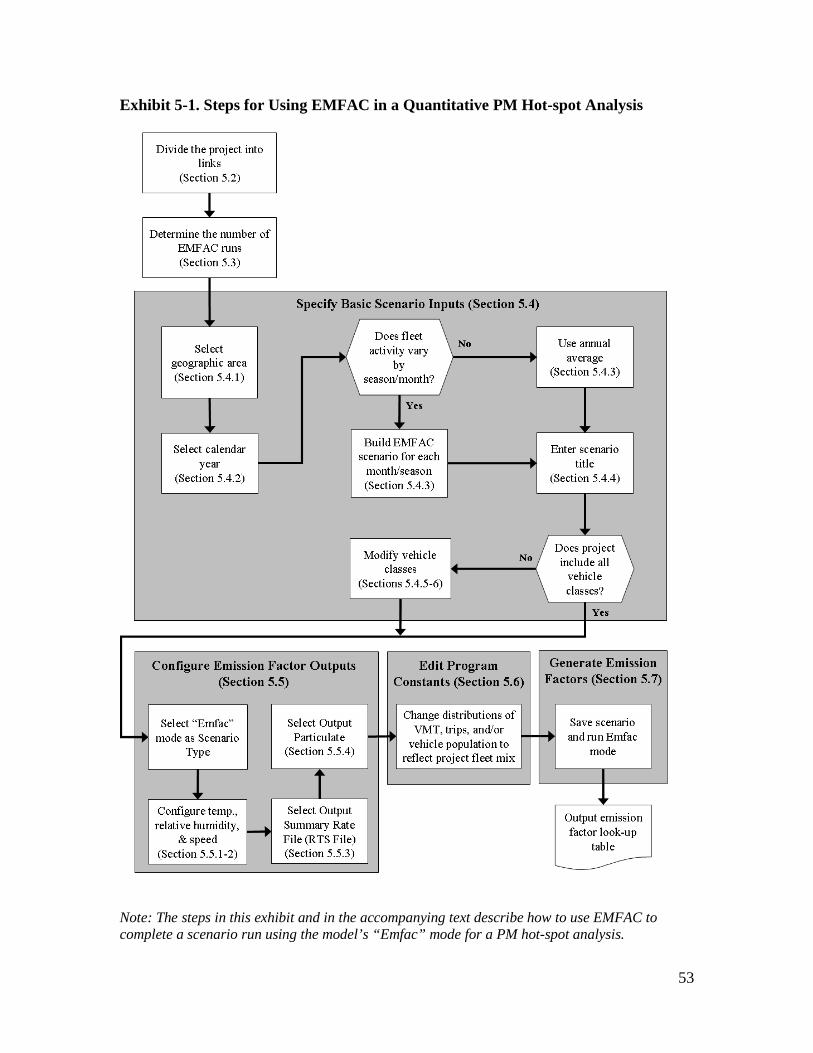
53

Exhibit 5-1. Steps for Using EMFAC in a Quantitative PM Hot-spot Analysis

Note: The steps in this exhibit and in the accompanying text describe how to use EMFAC to complete a scenario run using the model’s “Emfac” mode for a PM hot-spot analysis.

54

This section presumes users already have a basic understanding of how to run EMFAC. Please note that there are some aspects of Section 5 that differ from the MOVES guidance discussed in Section 4, due to the inherent differences between MOVES and EMFAC. For example, unlike MOVES, EMFAC emission rates do not vary by temperature. EMFAC users will not account for variations in temperature over the course of the day or year, and therefore will complete fewer model runs.58

Additionally, EMFAC generates an emission factor look-up table for a range of average speeds. MOVES calculates emission factors based on a distribution of operating modes, which allows the option of more advanced methods of defining link-level activity.

5.2 CHARACTERIZING A PROJECT IN TERMS OF LINKS Prior to using EMFAC, users need to first identify the project type and the associated emission processes (running, start, brake wear, tire wear, and idle exhaust) to be modeled. This guidance distinguishes between two types of transportation projects: (1) highway and intersection projects, and (2) transit or other terminal projects:

• For highway and intersection projects, running exhaust, brake wear, and tire wear emissions are the main focus.

• For transit and other terminal projects, start and extended idle emissions are typically needed, and in some cases these projects will also need to address cruise, approach and departure running exhaust emissions on affected links.

The goal of defining a project’s links is to accurately capture emissions where they occur. A link represents a segment of a highway or transit project characterized by a certain type of vehicle activity. Generally, the links specified for a highway project should include road segments with similar traffic conditions and characteristics. Links representing transit or other terminal projects should similarly reflect variation in idle and start activity, as well as other relevant cruise, approach and departure running exhaust emissions.

5.2.1 Highway and intersection projects General A PM hot-spot analysis fundamentally depends on the availability of accurate data on roadway link speed and traffic volumes for build and no-build scenarios.59

58 If future versions of EMFAC include PM emission rates that differ by temperature, EPA would work with CARB to develop additional EMFAC guidance as needed so that users could adequately capture hourly and seasonal temperature variability in PM hot-spot analyses.

Thus, local traffic data should be used to characterize each link sufficiently. It is recommended that

59 Project sponsors should document available traffic data sets, their sources, key assumptions, and the methods used to develop build and no-build scenario inputs for EMFAC. Documentation should include differences between how build and no-build traffic projections are obtained. For projects of local air quality concern, differences in traffic volumes and other activity changes between the build and no-build scenarios must be accounted for in the data that is used in the PM hot-spot analysis.

55

the user divide a project into separate links to allow sufficient resolution at different vehicle traffic and activity patterns; characterizing this variability in emissions within the project area will assist in air quality modeling (see Section 7). For analyses with EMFAC, an average speed and traffic volume is needed for each link.60

A simple example would be a single, one directional, four-lane highway that could be characterized as one link with one average speed. If the project analysis involves intersections, the intersections need to be treated separately from the free-flow links that connect to those intersections. Although road segments between intersections may experience free-flow traffic operations, the approaches and departures from the intersections will involve acceleration, deceleration, and idling activity not present on the free-flow link. For intersection modeling, the definition of link length will depend on the geometry of the intersection, how that geometry affects vehicle activity, and the level of detail of available activity information.

When using EMFAC, project sponsors can use average speeds for highway and intersection links based on travel time and distance. Travel time should account for the total delay attributable to traffic signal operation, including the portion of travel when the light is green and the portion of travel when the light is red. The effect of a red signal cycle on travel time includes deceleration delay, move-up time in a queue, stopped delay, and acceleration delay. Each approach link would be modeled as one link to reflect the higher emissions associated with vehicle idling through lower speeds affected by stopped delay; each departure link would be modeled as another link to reflect the higher emissions associated with vehicle acceleration through lower speeds affected by acceleration delay. Project sponsors should determine average congested speeds by using appropriate methods based on best practices used for highway analysis.61 Some resources are available through FHWA’s Travel Model Improvement Program (TMIP).62 Methodologies for computing intersection control delay are provided in the Highway Capacity Manual.63

5.2.2 Transit and other terminal projects

For transit and other terminal projects such as a bus terminal or intermodal freight terminal, the user should have information on starts per hour and number of vehicles idling during each hour. This activity will likely vary from hour to hour. It is

60 Unlike MOVES, the current version of EMFAC does not allow a user to account for more detailed data to describe the pattern of changes in vehicle activity (proportion of time in acceleration, deceleration, cruise, and idle activity) over the length of a road. 61 As discussed in Section 7, the use of the CAL3QHCR queuing algorithm for intersection idle queues is not recommended. Rather, idling vehicles should be represented in combination with decelerating, accelerating, and free-flow traffic on an approach segment of an intersection. 62 See FHWA’s TMIP website: http://tmip.fhwa.dot.gov/. 63 Users should consult the most recent version of the Highway Capacity Manual. As of the release of this guidance, the latest version is the Highway Capacity Manual 2000, which can be obtained from the Transportation Research Board (see http://144.171.11.107/Main/Public/Blurbs/152169.aspx for details).

http://tmip.fhwa.dot.gov/�

http://144.171.11.107/Main/Public/Blurbs/152169.aspx�

56

recommended that the user divide such a project into separate links to characterize variability in emission density within the project area appropriately (as discussed in Section 7). In this case, each “link” describes an area with a certain number of vehicle starts per hour, or a certain number of vehicles idling during each hour. Generally, users need to account for the number of vehicle starts and the amount of idle activity (in hours). Grams/trip rates can be calculated for start exhaust emissions. Additionally, grams/idle-hour (grams/hour) emission rates can be calculated for both regular idle and extended idle exhaust emissions, but only for heavy-duty vehicles. Users need to have data on the number of vehicle starts per hour and number of heavy-duty diesel vehicles idling during each hour to get the total project or project area emission factor. In addition, some transit and other terminal projects may have significant running emissions similar to free-flow highway projects (such as buses and trucks traveling to and from an intermodal terminal). These emissions can be calculated by defining one or more unique running links as described in Section 5.2.1 and Appendix G (that is, in addition to any other roadway links associated with the project). These running link emissions can then be aggregated with the emissions from starts and idling from non-running activity on the transit or other terminal link outside of the EMFAC model to generate the necessary air quality model inputs. Note: The user may choose to exclude sources such as a separate service drive, separate small employee parking lot, or other minor sources that are determined to be insignificant to project emissions.

5.3 DETERMINING THE NUMBER OF EMFAC RUNS 5.3.1 General Before running EMFAC to calculate emission factors, users should first determine the number of unique scenarios that can sufficiently describe activity variation in a project. In most projects, traffic volume, average speed, idling, fleet mix, and the corresponding emission factors will likely vary from hour to hour, day to day, and month to month. However, it is unlikely that data are readily available to capture such finite changes. Project sponsors may have activity data collected at a range of possible temporal resolutions. The conformity rule requires the use of latest planning assumptions or data available at the time the conformity analysis begins (40 CFR 93.110).64

64 See “

Depending on the sophistication of the activity data analysis for a given project, these data may range from a daily average-hour and peak-hour value to hourly estimates for all days of the year. EPA encourages the development of sufficient travel activity data to capture the expected ranges of traffic conditions for the build and no-build scenarios.

EPA and DOT Joint Guidance for the Use of Latest Planning Assumptions in Transportation Conformity Determinations,” EPA-420-B-08-901 (December 2008); available online at: www.epa.gov/otaq/stateresources/transconf/policy/420b08901.pdf.




57

5.3.2 Projects with typical travel activity data Traffic forecasts for highway and intersection projects are often completed for annual average daily traffic volumes, with an allocation factor for a daily peak-hour volume. This data can be used to conduct an analysis with EMFAC that is representative for all hours of the year. The most reasonable methods in accordance with good practice should be used to obtain the peak-hour allocation factors and diurnal distribution of traffic and the methods must be determined in accordance with interagency consultation procedures (40 CFR 93.105(c)(1)(i)). One option is to use average-hour and peak-hour traffic volumes to represent traffic over four time periods: morning peak (AM), midday (MD), evening peak (PM), and overnight (ON). For example, the peak-hour volume can be used to represent activity conditions over a three-hour morning (AM) and three-hour evening period (PM). The remaining 18 hours of the day can be represented by the average-hour volume. These 18 hours would be divided into a midday (MD) and overnight (ON) scenario. The following is one suggested approach for an analysis employing the average-hour/peak-hour traffic scenario:

• Morning peak (AM) emissions based on traffic data occurring between 6 a.m. and 9 a.m.;

• Midday (MD) emissions based on data from 9 a.m. to 4 p.m.; • Evening peak (PM) emissions based on data from 4 p.m. to 7 p.m.; and • Overnight (ON) emissions based on data from 7 p.m. to 6 a.m.

If there are local or project-specific data to suggest that the AM or PM peak traffic periods will occur in different hours than the default values suggested here, or over a longer or shorter period of time, that information should be documented and the hours representing each time period adjusted accordingly. Additionally, users should determine peak periods for the build and no-build scenarios independently and not assume that each scenario is identical. If the fleet mix does not vary between the peak-hour and average-hour, then only one EMFAC run is necessary. If there is a difference in fleet mix, two separate runs are necessary. 5.3.3 Projects with additional travel activity data Some project sponsors may have developed traffic or other activity data to show variations in volume and speed across hours, days, or months. Additionally, if users are modeling a transit or other terminal project, traffic volumes, starts, and idling estimates are likely to be readily available for each hour of the day. Under either of these circumstances, users have the option of applying the methodology described above (using average-hour and peak-hour as representative for all hours of the year) if it is determined through the interagency consultation process that using the additional data would not significantly impact the emissions modeling results. Alternatively, additional EMFAC

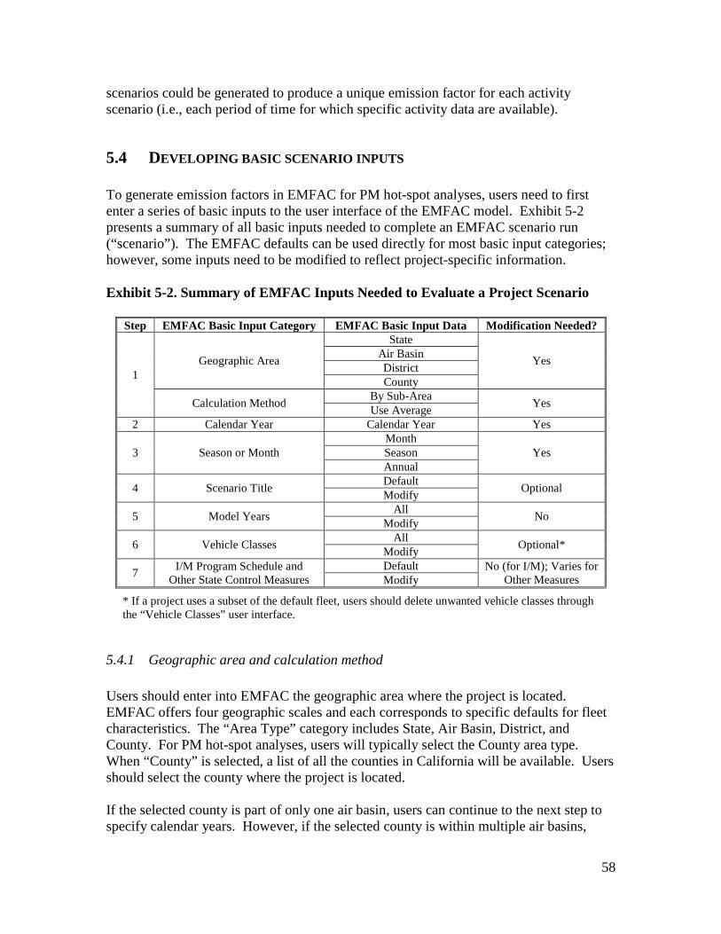
58

scenarios could be generated to produce a unique emission factor for each activity scenario (i.e., each period of time for which specific activity data are available).

5.4 DEVELOPING BASIC SCENARIO INPUTS To generate emission factors in EMFAC for PM hot-spot analyses, users need to first enter a series of basic inputs to the user interface of the EMFAC model. Exhibit 5-2 presents a summary of all basic inputs needed to complete an EMFAC scenario run (“scenario”). The EMFAC defaults can be used directly for most basic input categories; however, some inputs need to be modified to reflect project-specific information. Exhibit 5-2. Summary of EMFAC Inputs Needed to Evaluate a Project Scenario

Step EMFAC Basic Input Category EMFAC Basic Input Data Modification Needed?

1 Geographic Area

State

Yes Air Basin District County

Calculation Method By Sub-Area Yes Use Average 2 Calendar Year Calendar Year Yes

3 Season or Month Month

Yes Season Annual

4 Scenario Title Default Optional Modify

5 Model Years All No Modify

6 Vehicle Classes All Optional* Modify

7 I/M Program Schedule and Other State Control Measures

Default No (for I/M); Varies for Other Measures Modify

* If a project uses a subset of the default fleet, users should delete unwanted vehicle classes through the “Vehicle Classes” user interface.

5.4.1 Geographic area and calculation method Users should enter into EMFAC the geographic area where the project is located. EMFAC offers four geographic scales and each corresponds to specific defaults for fleet characteristics. The “Area Type” category includes State, Air Basin, District, and County. For PM hot-spot analyses, users will typically select the County area type. When “County” is selected, a list of all the counties in California will be available. Users should select the county where the project is located. If the selected county is part of only one air basin, users can continue to the next step to specify calendar years. However, if the selected county is within multiple air basins,

59

EMFAC will show two options, “By Sub-Area” and “Use Average,” as calculation methods. Users should select “By Sub-Area” to generate EMFAC emission factors in look-up tables for all sub-areas within the selected county. For instance, Los Angeles County is located in both the Mojave Desert Air Basin and the South Coast Air Basin. If the project is located near the Port of Los Angeles and “Los Angeles County” with “By Sub-Area” selected in EMFAC runs, EMFAC will provide emission data for both the Mojave Desert Air Basin and the South Coast Air Basin. Only the look-up tables for the South Coast Air Basin would be used because this is where the port is located; the Mojave Desert Air Basin data would be ignored.

5.4.2 Calendar year EMFAC is able to analyze calendar years from 1970 to 2040 and allows emission calculations for multiple calendar years in a single run. Users should select one or more calendar years in EMFAC based on the project scenarios to be analyzed. If an analysis year beyond 2040 is needed, select 2040 to represent that year.

5.4.3 Season or month EMFAC can estimate emission factors for each month, two seasons (winter and summer), or an annual average. Although VMT and speed are handled external to the model, the vehicle mix may vary by hour and season and these scenarios should be modeled explicitly. As discussed in Section 5.3, users should run EMFAC for the appropriate number of scenarios based on the availability of travel activity data. Users with typical travel activity data may run one or two scenarios (depending whether vehicle mix varies between the peak-hour and average-hour) and will select “annual average” in the “Season or Month” selection panel. Users with additional data that shows variation in fleet mix across seasons or months should select the appropriate month or season for each run.

5.4.4 Scenario title EMFAC generates a default scenario title that includes the name of the county, calculation method, season or month, and calendar year. A replacement scenario title can be specified, if desired.

5.4.5 Model years EMFAC includes vehicle model years from 1965 to 2040 and default assumptions about mileage accumulation that vary by model year. EMFAC will generate emission factors for 45 model years (ages 1 through 45) for the build and no-build scenarios for each analysis year. Users can change the range of model years to be included in an EMFAC run through the model interface. If a project involves a specialized and simple fleet (e.g., buses operating in a bus terminal) for which the range of model years is well known or reliably estimated, users may consider including only those model years and exclude unrelated vehicle types in an EMFAC run.

60

However, under most circumstances, projects that involve multiple vehicle types and model years will need EMFAC defaults to be used for PM hot-spot analyses. The two reasons for this recommendation are: (1) most projects will not affect the age distribution of the vehicles operating at the project site, and (2) changing EMFAC defaults to reflect specific fleet age distributions is complicated for projects that involve multiple vehicle types and model years. These changes involve a level of familiarity with EMFAC that many users may not have or need for most hot-spot analyses. Therefore, if users anticipate that it will be necessary to adjust the age distribution of their vehicle fleet, they should consult with CARB for further guidance.

5.4.6 Vehicle classes All 13 default vehicle classes should be selected for most projects. The exception would be a project or link that involves a specialized fleet of limited vehicle types (e.g., a bus terminal). The EMFAC model assumes vehicle population and travel activity distributions by vehicle class, depending on the geographic area and analysis year selected. Editing the default distribution of vehicle classes will be discussed in Section 5.5. If only one vehicle type is selected (e.g., heavy-heavy duty trucks (HHDTs)), all emission information in the EMFAC output will be calculated for that one vehicle type.

5.4.7 I/M program schedule and other state control measures When a particular county from the Geographic Area panel is selected in EMFAC, the model assumes a default I/M program. Although EMFAC allows edits for each I/M program, users should not alter the default settings and parameters associated with I/M programs and their coverage. If I/M program modifications are considered, users should consult with the local air district or CARB for specific guidance. Currently, no PM emission benefit from I/M programs exists in EMFAC2007. The PM emission reductions from any additional state PM emission control measure should be applied outside of the EMFAC model and be consistent with current implementation of measures and how reductions are calculated for SIP and other air quality planning purposes. For instance, EMFAC2007 currently does not have the capability of modeling diesel engine retrofits. It is recommended that manufacturer specification data be used for calculating emission factors from engines equipped with such devices, consistent with EPA’s and CARB’s retrofit guidance and methods used to calculate reductions for the SIP. Any issues regarding the models and associated methods and assumptions for the inclusion of state control measures in PM hot-spot analyses must be considered through the process established by each area’s interagency consultation procedures (40 CFR 93.105(c)(1)(i)).65

65 For information about quantifying the benefits of retrofitting diesel vehicles and engines to conformity determinations, see EPA’s website for the most recent guidance on this topic:

www.epa.gov/otaq/stateresources/transconf/policy.htm. Also, see CARB’s website at: www.arb.ca.gov/msprog/onrdiesel/calculators.htm.


http://www.arb.ca.gov/msprog/onrdiesel/calculators.htm�

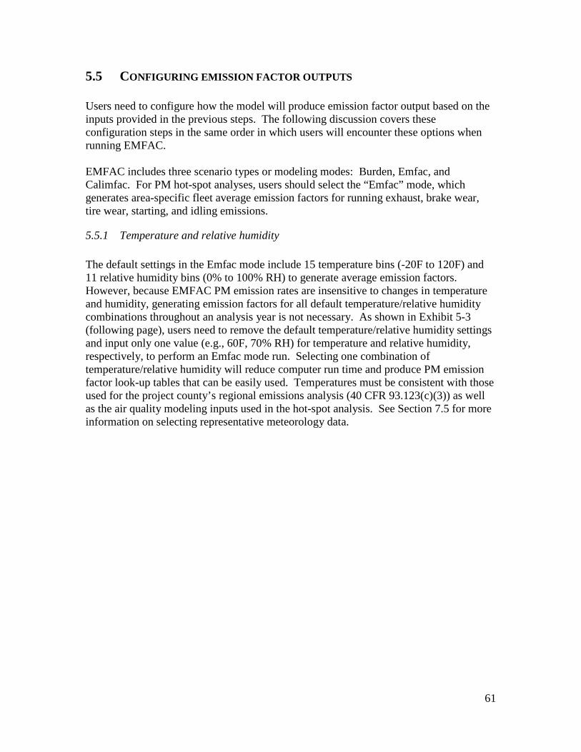
61

5.5 CONFIGURING EMISSION FACTOR OUTPUTS Users need to configure how the model will produce emission factor output based on the inputs provided in the previous steps. The following discussion covers these configuration steps in the same order in which users will encounter these options when running EMFAC. EMFAC includes three scenario types or modeling modes: Burden, Emfac, and Calimfac. For PM hot-spot analyses, users should select the “Emfac” mode, which generates area-specific fleet average emission factors for running exhaust, brake wear, tire wear, starting, and idling emissions.

5.5.1 Temperature and relative humidity The default settings in the Emfac mode include 15 temperature bins (-20F to 120F) and 11 relative humidity bins (0% to 100% RH) to generate average emission factors. However, because EMFAC PM emission rates are insensitive to changes in temperature and humidity, generating emission factors for all default temperature/relative humidity combinations throughout an analysis year is not necessary. As shown in Exhibit 5-3 (following page), users need to remove the default temperature/relative humidity settings and input only one value (e.g., 60F, 70% RH) for temperature and relative humidity, respectively, to perform an Emfac mode run. Selecting one combination of temperature/relative humidity will reduce computer run time and produce PM emission factor look-up tables that can be easily used. Temperatures must be consistent with those used for the project county’s regional emissions analysis (40 CFR 93.123(c)(3)) as well as the air quality modeling inputs used in the hot-spot analysis. See Section 7.5 for more information on selecting representative meteorology data.

62

Exhibit 5-3. Changing EMFAC Default Settings for Temperature and Relative Humidity

5.5.2 Speed The Emfac mode allows users to input up to 24 speed values to populate average emission factors. The default setting specifies speed bins for 0 mph through 65 mph in 5 mph increments. Emission factors associated with the 0 mph speed bin can be applied for idle emissions (essentially for heavy-duty trucks only; EMFAC idle emission factors are unavailable for most other vehicle classes).66

Emission factors for intermediate speeds can also be generated if specific speed values are input into the EMFAC model.

Users have several options to calculate appropriate speed-dependent emission factors for a project. For instance, if a highway link in a build scenario is known to have an average speed of 32 mph, it can be directly input into the speed list of EMFAC to produce the associated PM emission factors. Alternatively, if the EMFAC default settings are used to generate a look-up table for different speed bins, users can either select the emission

66 Among the 13 vehicle classes in EMFAC, idle emission factors are available only for LHDT1 and LHDT2 (included in the MDT vehicle group in the output .rts file) and MHDT, HHDT, School Buses, and Other Buses (included in the HDT vehicle group in the output .rts file); see Exhibit 5-6 for further information.

63

factors associated with the closest speed bin (e.g., 30 mph bin, representing speeds of 27.5 mph to 32.5 mph), or interpolate between the emission factors for speed bins of 30 mph and 35 mph. Users should include 0 mph in an EMFAC run unless the project to be evaluated does not involve idle emissions. For specific cases for which the average link speed is less than 5 mph, users can either select the emission factors from the 5 mph speed bin, or extrapolate down to the desired speed by using the emission factors from the speed bins for 5 mph and 10 mph to create a trend line to lower speeds.

5.5.3 Output rate file The Emfac mode can provide emission information in four output formats with different levels of detail. Users should select “Summary Rates (RTS).” The Summary Rates format generates average emission factors by speed for six vehicle groups (aggregated from the 13 vehicle classes modeled in EMFAC) and an overall average emission factor for the entire vehicle fleet. The overall average emission factors are appropriate for use in air quality dispersion modeling.

5.5.4 Output particulate As shown in Exhibit 5-4, users have to select either PM10 or PM2.5 in an Emfac mode run to obtain particulate emission factors. EMFAC must be run twice to obtain both PM10 and PM2.5 data for those projects that are located in both PM10 and PM2.5 nonattainment/maintenance areas. Exhibit 5-4. Selecting Pollutant Types in EMFAC for PM10 and PM2.5

64

5.6 EDITING PROGRAM CONSTANTS

5.6.1 Overview Typically, users will start the analysis process with only a broad understanding of the project-specific vehicle fleet – specifically, the percentage of vehicles that are considered “trucks” versus those that are “non-trucks.” In all cases, projects that require a quantitative PM hot-spot analysis will have a different fleet distribution than the EMFAC regional default mix. Users will therefore need to adjust the project fleet and fleet activity (VMT, trips) to reflect the expected project fleet mix for each EMFAC scenario. Depending on the project, users should modify some combination of VMT (which affects running exhaust emission factors), vehicle trips (which affects starting emission factors), and/or vehicle population (which affects idling emission factors). In the following discussion, overall guidance is provided on how to make these adjustments. Appendices G and H provide more specific illustrations of the step-by-step procedures involved.

5.6.2 Default data in the Emfac mode The Emfac mode is associated with a range of pre-populated program constants linked to specific time periods and California geographic areas. Exhibit 5-5 lists the default data available in the Emfac mode that can be accessed through the “Edit Program Constants” in the user interface. For a PM hot-spot analysis, many of the defaults do not need to be modified. However, users do need to determine which adjustments are needed for the default distributions of VMT, trips, and vehicle population by vehicle class. The EMFAC interface has “Copy with Headers” and “Paste Data Only” tabs that are helpful for users to easily export the default data and import the adjusted data. Exhibit 5-5. EMFAC Program Constants and Modification Needs for PM Hot-spot Analyses

EMFAC Program Constants Description

Modification Needed for PM

Analyses? Exh Tech Fractions Exhaust control technology fractions No Evap Tech Fractions Evaporative control technology factions No Interim I/M Enhanced interim I/M program No Population Vehicle population by class, fuel type, and age Yes* Accrual Odometer accrual rate by class, fuel type, and age No Trips Vehicle trips/starts per day by class, fuel type, and age Yes* VMT Vehicle miles traveled per day by class, fuel type, and age Yes* Speed Fractions VMT by speed bin distribution for each vehicle class No Idle Time Idle times by vehicle class, fuel, and hour of day No

* Different distributions in VMT, trips, or vehicle population than those reflected by the EMFAC defaults should be updated through the user interface to incorporate project-specific vehicle activity information.

65

5.6.3 Comparing project data and EMFAC defaults to determine adjustments Individual projects will have a mix of vehicle types that varies from the regional average fleet mix. Because PM hot-spot analyses can be especially sensitive to diesel-powered truck activity, it is important to characterize the relative fraction of the fleet that is comprised of trucks compared to light-duty vehicles properly. Users should determine the base (default) case and forecasted vehicle mix (trucks versus non-trucks) applicable to their project’s build and no-build scenarios and use that information to adjust EMFAC defaults. Users should first collapse VMT, vehicle trip and vehicle population data for EMFAC’s 13 vehicle classes to two general data categories: “truck” and “non-truck.” The common practice in California is to define, for emission purposes, “truck” activity as being comprised of all activity associated with what EMFAC identifies as medium-duty and heavier vehicles. In addition, travel activity data typically identify “trucks” in a general sense, without regard to their fuel type. Exhibit 5-6, therefore, shows the suggested vehicle class mapping given the likely data available at the project level. Exhibit 5-6. Mapping EMFAC Vehicle Classes to Project-specific Activity Information

Typical Projects (2 categories)

EMFAC Default

(13 classes) Description

EMFAC Output Summary Rates (RTS)

File (6 groups)

Non-truck LDA Passenger cars LDA LDT1 Light-duty trucks 1 LDT LDT2 Light-duty trucks 2 MCY Motorcycles MCY

Truck MDV Medium-duty trucks MDT LHDT1 Light-heavy-duty trucks 1 LHDT2 Light-heavy-duty trucks 2 MHDT Medium-heavy-duty trucks HDT HHDT Heavy-heavy-duty trucks MH Motor homes OBUS Other buses SBUS School buses UBUS Urban buses UBUS

5.6.4 Adjustment of default activity distributions to reflect project data After the vehicle mapping is complete, users will need to compare the project-specific distributions to the default data included in EMFAC for trucks and non-trucks. For example, assume 2009 is used as the analysis year for a hypothetical highway project in Sacramento County with 25% of total annual average daily VMT apportioned to trucks. After entering all the basic inputs in the EMFAC modeling software, pre-populated (default) county VMT for the truck portion of the fleet is equal to 6,269,545 (when all

66

appropriate vehicle classes are summed up), and the model default activity shows that truck VMT represents 19% of total VMT in Sacramento County (see Exhibit 5-7).

The VMT should then be re-allocated to the correct percentage. EMFAC allows users to adjust the calculated fleet-average emission factors by varying the relative weightings of the 13 vehicle classes. This adjustment is done by replacing the default numbers for each vehicle class in the EMFAC user interface, using the “VMT” option for a highway project, or the “Trips” or “Population” option if analyzing a transit or other terminal project, under the “Edit Program Constants” function available via the Emfac mode screen. Note: EMFAC also allows users to modify the fuel characteristics (gas/diesel/electric) for each of the 13 vehicle classes. For most PM hot-spot analyses for highway projects with non-captive fleets, users will not need to modify the fuel assumed for the fleet vehicles. For projects involving captive fleets with known fuel use distributions, the default fractions should be modified. Exhibit 5-7. Example Default EMFAC VMT by Vehicle Class Distribution

Continuing with the Sacramento County illustration from the previous step, users would need to scale the EMFAC defaults to reflect the truck/non-truck VMT fractions appropriate to the project (i.e., truck VMT needs to be adjusted from 19% to 25% of the total). The fractional differences for trucks and non-trucks are then applied to the default VMT for each corresponding vehicle class in the EMFAC user interface. As illustrated

67

in Exhibit 5-8, when the VMT values for the truck classes are adjusted, their sum is equal to 8,101,117 (25% of total county VMT). Adjusted non-truck VMT is now 24,303,350 (75% of total VMT). The details of this example are presented in Appendix G. When updating the EMFAC default VMT by vehicle class, the total VMT (for all 13 vehicle classes) must remain unchanged. Exhibit 5-8. Example Adjusted EMFAC VMT by Vehicle Class Distribution

Note that, in special cases, if one or more of the default vehicle classes are not present in the project area, users should set VMT (to address running exhaust emissions), number of trips (to address starting emissions) and population (to address idling emissions) for that class to “1” in the EMFAC interface. In other words, users should functionally zero-out the appropriate vehicle class by inputting a value of “1” because EMFAC does not allow an input of zero in the interface for VMT, trip, and vehicle population distributions. A complete example illustrating how to change EMFAC default distributions to exclude some vehicle classes for a transit project is presented in Appendix H. An alternate way is to delete unwanted vehicle classes in the basic scenario data input to the model. Appendices G and H provide more detailed examples of these steps; these modifications will typically only be necessary for projects involving unique conditions such as truck-only activity.

68

Note: The average emission factors provided by EMFAC in the “Emfac mode” are VMT-weighted (for running emissions), vehicle trip-weighted (for start emissions), or vehicle population-weighted (for idle emissions) across different vehicle classes. If a user runs the model for a county, the weighting reflects county-level VMT, trips (starts), or vehicle fleet and their absolute values are not relevant at the project level. For most transit and other terminal projects, users may have very detailed information on not only vehicle mix, but also fuel mix (diesel/gas/electric) and age distribution (model year distribution). Users should adjust the fuel mix (changed through the “By Vehicle and Fuel” tabs of the VMT, Population, and Trips panels) to reflect the known or expected fuel use (if, for instance, a bus fleet is expected to use entirely diesel fuel). Similarly, if the age distribution (model year distribution) is known for a particular fleet, this should be entered in place of the EMFAC default values (found in the “By Vehicle/Fuel/Age” tab of the Edit Population panel). Note that EMFAC’s ability to model alternate fuel options is not uniform among vehicle classes. If users determine that modification of the fleet in terms of fuel or age distribution is needed, they should contact CARB for further guidance. However, for most highway and intersection projects with a non-captive fleet, the EMFAC default fuel mix and age distribution should be used.

5.7 GENERATING EMISSION FACTORS FOR USE IN AIR QUALITY MODELING

For each EMFAC run, emission factors will be generated in the “Summary Rates (RTS)” file (.rts file) in the form of look-up tables. These tables are organized and numbered by different emission processes and pollutant types. PM emission factors for running exhaust, idle exhaust, tire wear, and brake wear are included in Table 1 of the .rts file; PM start emission factors are included in Table 2 of the .rts file. Exhibit 5-9 (following page) includes example screenshots of EMFAC .rts file output.

5.7.1 Highway and intersection links For each speed value (greater than 0 mph), EMFAC outputs running exhaust, tire wear, and brake wear emission factors in grams/vehicle-mile, for six vehicle groups plus an aggregate emission factor named as “All” (see Exhibit 5-6). Note that the .rts output file includes only six vehicle groups – an aggregation of the 13 vehicle classes manipulated during the input process. In general, assuming users have run the model with VMT-weighted distributions appropriate for the project’s fleet activity (see Section 5.6), only the emission factors from the “All” column will be needed. The “All” column includes a grams/vehicle-mile value that is a VMT-weighted average based on the user-provided vehicle activity mix. The sum of running exhaust, tire wear, and brake wear grams/mile PM emission factors for a given speed is the total fleet-average grams/vehicle-mile emission factor appropriate for modeling highway project links:

Total Link Emission Factor = (EFrunning) + (EFtire wear) + (EFbrake wear)

69

The total link emission factor (grams/vehicle-mile) can be used in combination with the link volume and link length as input into CAL3QHCR. If using AERMOD, an emission rate (in grams/hour) should be calculated for each link. This can be done by multiplying the total link emission factor (calculated above) by the link hourly volume and link length. Exhibit 5-9. Example EMFAC Running Exhaust, Tire Wear, and Brake Wear Emission Factors in the Summary Rates (rts) Output File

70

5.7.2 Transit and other terminal links For transit and other terminal projects, such as bus terminals or intermodal freight terminals, grams/trip (or grams/start) emission factors can be combined with project-specific estimates of vehicle trips (or starts) per hour to calculate grams/hour emissions. Starting emission factors depend on the vehicle soak time (the soak time is the time a vehicle is stationary with the engine turned off, following the last time it was operated). The longer a vehicle is turned off, or soaks, the higher the start emissions embedded in EMFAC. The output look-up table for start emissions includes 18 time bins (5 minutes to 720 minutes); users need to choose an appropriate time bin that is representative for the project activity. Selected examples of some potential associated soak times are shown in Exhibit 5-10 for several possible scenarios.

Exhibit 5-10. Example Soak Times for Several Project Scenarios

Project Type Example Soak Time

(min)* PM10 Start Emission

Factors (g/trip) Bus Transit Facility 10 0.002 Truck Refueling Station 60 0.008 Intermodal Distribution Center 180 0.013 Truck Stop Parking Lot 480 0.016

* Example soak times and emission factors are for illustration purposes and are not to be used as literal values. Users should select soak times and estimate emission factors appropriate to the specific project and implementation dates to be evaluated. Emission factors will vary by analysis year.

Idling emission factors are in grams/idle-hour and are available in Table 1 of the .rts file associated with a speed value of 0 mph (available only for MDT and HDT groups due to EMFAC’s data limitations). Note that, for transit and other terminal projects, idling and starting emission factors from EMFAC should not be combined directly because they are generated in different units. The project idling and starting emissions (in grams) need to be calculated separately for a particular time period, based on project-specific idle hour and trips/hour data. The total transit or other terminal project emissions for the time period are the sum of the two values:

Total Project Emissions = (EFidling * idle hours) + (EFstarting * trips) The result of this calculation is a grams/hour emission rate that can be used for air quality modeling. In some cases, users may need to model running exhaust emissions from cruise, approach, and departure link activity, as well as start and idle emissions at the project site. For instance, to assess impacts from a proposed bus terminal, users may need to evaluate both the start and idle emissions from buses at the terminal as well as the bus running exhaust emissions along the links approaching and departing from the terminal. Given that the link activity will involve a unique vehicle fleet (one with a disproportionate amount of bus activity), users should modify the default travel activity

71

in EMFAC to reflect the bus activity (see the discussion above). EMFAC allows users to generate emission factors for both the approaching/departing links and the bus terminal itself in a single run. To obtain project-specific running exhaust emission factors, users can modify the VMT associated with the buses at the approaching link by adjusting the values for each of the 13 vehicle classes in the user interface with the method described in Section 5.6. In the same EMFAC run, users can enter project-specific vehicle population and trip distributions to produce project-specific start and idle emission factors. Another special case may involve modeling idling emissions for a specific fleet of heavy heavy-duty diesel trucks (HHDT). Because EMFAC provides only an overall average idle emission factor for heavy-duty trucks regardless of fuel type, ambient conditions, accessory usage, and engine speed, CARB has created supplemental guidance that, off-model, provides season-specific HHDT emission factors for activity that CARB has termed “high idle” and “low idle.”67

Low idle (sometimes also called “curb idle”) involves short-term idling with engine speeds of 800 rpm or less and no accessory loading. High idle is idling over an extended period of time with engine speeds over 800 rpm, usually involving the use of heaters, air conditioners, or other vehicle accessories. If the project under evaluation involves HHDT and the user has detailed information about the fleet (vehicle model years and the amount of time spent in low and high idle, in particular), the information from this supplemental guidance may be used to obtain more specific idle emission factors for HHDT than would otherwise be available by simply using EMFAC.

Other special projects may need additional data manipulation. Project sponsors should contact CARB or the local air quality management district for further guidance. Note: The product of any transit or other terminal project should be a grams/hour emission factor for each defined project area. If approach/departure running emissions are calculated, a grams/hour emission factor should be calculated from the grams/mile EMFAC output as described in Section 5.7.1. Alternative Method to Estimate Idle and Start Emission Factors for a Specific Vehicle Class A relatively simple method is available to obtain idle and start emission factors for those cases in which users are interested in only one vehicle class (such as for heavy-duty trucks). Note that this method is not recommended for situations involving multiple vehicle classes (e.g., medium- and heavy-duty trucks). Because this is a methodology to support development of idle and start emission factors, it is applicable only to those vehicle classes for which EMFAC includes idle emissions (LHDT1, LHDT2, MHDT, HHDT, School Buses, and Other Buses).

67 See EMFAC Modeling Change Technical Memo, “Revision of Heavy Duty Diesel Truck Emissions Factors and Speed Correction Factors” (original and amendment), October 20, 2006; available through ARB online at: www.arb.ca.gov/msei/supportdocs.htm#onroad.

http://www.arb.ca.gov/msei/supportdocs.htm#onroad�

72

For example, suppose a project or link involves just HHDT. In this case, users could modify EMFAC’s basic input of Vehicle Classes in Section 3.6 in the user interface and select “Heavy Heavy Duty Trucks.” Editing EMFAC default population and trip distributions is not needed because the output .rts file will reflect emission factors that are associated with the selected single vehicle class only.

73

Section 6: Estimating Emissions from Road Dust, Construction, and Additional Sources

6.1 INTRODUCTION This section provides guidance on how to estimate re-entrained road dust and transportation-related construction dust emissions. MOVES and EMFAC do not estimate emissions of road or construction dust, so this section must be consulted if dust is required to be included in the PM hot-spot analysis. See Section 2.5 for further information regarding when dust emissions are required to be included in a PM hot-spot analysis. This section also includes information on quantifying emissions from construction vehicles and equipment and additional sources in the project area, when applicable. The models and associated methods and assumptions used in estimating these emissions must be evaluated and chosen through the process established by each area’s interagency consultation procedures (40 CFR 93.105(c)(1)(i)).

6.2 OVERVIEW OF DUST METHODS AND REQUIREMENTS In summary, road or construction dust can be quantified using EPA’s AP-42 method or alternative local methods. AP-42 is EPA’s compilation of data and methods for estimating average emission rates from a variety of activities and sources from various sectors. Refer to EPA’s website (www.epa.gov/ttn/chief/ap42/index.html) to access the latest version of AP-42 sections and for more information about AP-42 in general. The sections of AP-42 that address emissions of re-entrained road dust from paved and unpaved roads and emissions of construction dust are found in AP-42, Chapter 13, “Miscellaneous Sources.” The key portions of the chapter include:

• Section 13.2: “Introduction to Fugitive Dust Sources,” • Section 13.2.1: “Paved Roads” • Section 13.2.2: “Unpaved Roads” • Section 13.2.3: “Heavy Construction Operations” (includes road construction)

Users should consult EPA’s website to ensure they are using the latest approved version of AP-42, as the methodology and procedures may change over time.68

In addition to the latest version of AP-42, alternative local methods can be used for estimating road or construction dust; in some areas, these methods may already exist and can be considered for use in quantitative PM hot-spot analyses. This section presumes users already have a basic understanding of how to use AP-42 or other dust methods.

68 This guidance is applicable to current and future versions of AP-42, unless otherwise noted by EPA in the future.

http://www.epa.gov/ttn/chief/ap42/index.html�

74

6.3 ESTIMATING RE-ENTRAINED ROAD DUST

6.3.1 PM2.5 nonattainment and maintenance areas The transportation conformity rule requires a hot-spot analysis in a PM2.5 nonattainment and maintenance area to include emissions from re-entrained road dust only if emissions from re-entrained road dust are determined to be a significant contributor to the PM2.5 nonattainment problem. See Section 2.5 for further information.

6.3.2 PM10 nonattainment and maintenance areas Re-entrained road dust must be included in all PM10 hot-spot analyses. EPA has historically required road dust emissions to be included in all conformity analyses of direct PM10 emissions – including hot-spot analyses. See Section 2.5 for further information.

6.3.3 Using AP-42 for road dust on paved roads Section 13.2.1 of AP-42 provides a method for estimating emissions of re-entrained road dust from paved roads for situations for which silt loading, mean vehicle weight, and mean vehicle speeds on paved roads fall within ranges given in AP-42, Section 13.2.1.3 and with reasonably free-flowing traffic (if the project doesn’t meet these conditions, see Section 6.3.5, below). Section 13.2.1 of AP-42 contains predictive emission factor equations that can be used to estimate an emission factor for road dust. This section can be downloaded from EPA’s website at: www.epa.gov/ttn/chief/ap42/ch13/index.html. When estimating emissions of re-entrained road dust from paved roads, site-specific silt loading data must be consistent with the data used for the project’s county in the regional emissions analysis (40 CFR 93.123(c)(3)). In addition, if the project is located in an area where anti-skid abrasives for snow-ice removal are applied, information about their use should be included (e.g., the number of times such anti-skid abrasives are applied).

6.3.4 Using AP-42 for road dust on unpaved roads Section 13.2.2 of AP-42 provides a method for estimating emissions of re-entrained road dust from unpaved roads. Different equations are provided for vehicles traveling unpaved surfaces at industrial sites and vehicles traveling on publicly accessible roads. Most PM hot-spot analyses will involve only vehicles traveling on publicly accessible roads. When applying an equation that accounts for surface material moisture content, the percentage of surface material moisture must be consistent with the data used for the project’s county in the regional emissions analysis (40 CFR 93.123(c)(3)).

http://www.epa.gov/ttn/chief/ap42/ch13/index.html�

75

6.3.5 Using alternative local approaches for road dust Some PM areas have historically used locally-developed methods for estimating re-entrained road dust emissions that may be more appropriate than the AP-42 methods given specific local conditions. Other areas may develop alternatives in the future. Also, an alternative method could be used if the equations in AP-42 do not apply to a particular project, as they were developed using a particular range of source conditions. Section 13.2.1 of AP-42 currently states that users should use caution when applying the 13.2.1 equation outside of the range of variables and operating conditions specified. In these cases, users are encouraged to consider alternative methods that can better reflect local conditions.

6.4 ESTIMATING TRANSPORTATION-RELATED CONSTRUCTION DUST

6.4.1 Determining whether construction dust must be considered Construction-related PM2.5 or PM10 emissions associated with a particular project are required to be included in hot-spot analyses only if such emissions are not considered temporary as defined in 40 CFR 93.123(c)(5) (see Section 2.5.5). The following discussion includes guidance only for construction-related dust emissions; any other construction emissions (e.g., exhaust emissions from construction equipment) would need to be calculated separately, as discussed in Section 6.6.

6.4.2 Using AP-42 for construction dust Section 13.2.3 of AP-42 describes how to estimate emissions of dust from construction of transportation projects. This section can be downloaded from EPA’s website at: www.epa.gov/ttn/chief/ap42/ch13/index.html. Section 13.2.3 of AP-42 indicates that a substantial source of construction-related emissions could be from material that is tracked out from the site and deposited on adjacent paved streets. Therefore, AP-42 states that persons developing construction site emission estimates need to consider the potential for increased adjacent emissions from off-site paved roadways; users should refer to the discussion regarding paved roads in Section 6.3.3.

6.4.3 Using alternative approaches for construction dust Some PM nonattainment or maintenance areas have historically used alternative methods for estimating construction dust that may be more appropriate than AP-42, given specific local conditions. Other areas may develop alternatives in the future. Also, an alternative method may be more appropriate if the project’s conditions – such as surface material silt and moisture content percentages, mean vehicle weight and speed – are not within the ranges of source conditions that were tested in developing the

http://www.epa.gov/ttn/chief/ap42/ch13/index.html�

76

equations. In such cases, users may consider alternative methods that are more appropriate for local conditions.

6.5 ADDING DUST EMISSIONS TO MOVES/EMFAC MODELING RESULTS Emission factors for road and construction dust should be added to the emission factors generated for each link by MOVES or EMFAC (in California). Once this data is available, the user can move on to Section 7 to develop input files for the appropriate air quality model.

6.6 ESTIMATING ADDITIONAL SOURCES OF EMISSIONS IN THE PROJECT AREA

6.6.1 Construction-related vehicles and equipment In certain cases, emissions resulting from construction vehicles and equipment, including exhaust emissions as well as dust, must be included in an analysis; refer to Section 2.5.5 for more information on when to include such emissions. State and local air agencies may have quantified these types of emissions for the development of SIP non-road mobile source inventories, and related methods should be considered for PM hot-spot analyses. Evaluating and choosing models and associated methods and assumptions for quantifying construction-related emissions must be determined through an area’s interagency consultation procedures (40 CFR 93.105(c)(1)(i)).

6.6.2 Locomotives EPA has developed guidance to quantify locomotive emissions when they are a component of a transit or freight terminal or otherwise a source in the project area being modeled. See Appendix I for further general guidance, resources, and examples.

6.6.3 Additional emission sources When applicable, additional sources need to be estimated and included in air quality modeling, as described in Section 8.

77

Section 7: Selecting an Air Quality Model, Data Inputs, and Receptors

7.1 INTRODUCTION This section describes the recommended air quality models, data inputs, and receptor considerations for PM hot-spot analyses. This guidance is consistent with the conformity rule and recommendations for air quality modeling in EPA’s “Guideline on Air Quality Models” (Appendix W to 40 CFR Part 51). Regardless of the model used, the quality of a model’s predictions depends on appropriate input data, proper formatting, model setup, quality assurance, and other assumptions. As noted in Section 2, air quality modeling for PM hot-spot analyses must meet the conformity rule’s general requirements for such analyses (40 CFR 93.123(c)) and rely on the latest planning assumptions available when the conformity analysis begins (40 CFR 93.110). This section presumes that users already have a basic understanding of air quality models and their operation. EPA has also included additional details on air quality modeling in Appendix J of this guidance. The models in this section, user guides, and supporting documentation are available through EPA’s Support Center for Regulatory Air Models (SCRAM) website at: www.epa.gov/scram001. Project sponsors conducting PM hot-spot analyses will need to refer to the latest user guides and available guidance for complete instructions.

7.2 GENERAL OVERVIEW OF AIR QUALITY MODELING Air quality models, methods, and assumptions need to be determined for each PM hot-spot analysis through the interagency consultation process (40 CFR 93.105(c)(1)(i)). Exhibit 7-1 (following page) outlines the basic process for conducting air quality modeling for a given project. This exhibit depicts the flow of information developed for air quality modeling (as described in this section), the development of background concentration estimates (see Section 8), and the calculation of design values and comparison to the NAAQS (see Section 9).

http://www.epa.gov/scram001�

78

Exhibit 7-1. Overview and Data Flow for Air Quality Modeling

79

7.3 SELECTING AN APPROPRIATE AIR QUALITY MODEL

7.3.1 Recommended air quality models

PM hot-spot analyses should be developed consistent with EPA’s current recommended models under Appendix W to 40 CFR Part 51. The purpose of recommending a particular model is to ensure that the best-performing methods are used in assessing PM impacts from a particular project and are employed in a consistent fashion.69

Exhibit 7-2 summarizes the recommended air quality models for PM hot-spot analyses for required projects under 40 CFR 93.123(b)(1).

Exhibit 7-2. Summary of Recommended Air Quality Models

Type of Project Recommended Model

Highway and intersection projects AERMOD, CAL3QHCR

Transit, freight, and other terminal projects AERMOD

Projects that involve both highway/intersections and terminals, and/or nearby sources* AERMOD

* Note that “nearby sources” refers to those sources that (1) are not part of the project but are affected by the project or (2) are sources in the project area whose emissions are not adequately captured by the selected background concentrations. See Section 8.2 for more information. The American Meteorological Society/EPA Regulatory Model (AERMOD) is EPA’s recommended near-field dispersion model for many regulatory applications. EPA recommended AERMOD in a November 9, 2005 final rule that amended EPA’s “Guideline on Air Quality Models” after more than ten years of development and peer review that resulted in substantial improvements and enhancements.70

69 The best performing model is one that best predicts regulatory design values for a particular pollutant. EPA’s “Protocol for Determining the Best Performing Model” (EPA-454/R-92-025) defines operational and statistical criteria for this evaluation. According to the document: “For a pollutant…for which short-term ambient standards exist, the statistic of interest involves the network-wide highest concentration…the precise time, location, and meteorological condition is of minor concern compared to the magnitude of the highest concentration actually occurring.”

AERMOD includes options for modeling emissions from volume, area, and point sources and can therefore model the impacts of many different source types, including highway and transit projects. In addition, EPA conducted a study to evaluate AERMOD and other air quality models in preparation for developing this guidance and the study supported

70 The final rule can be found at: www.epa.gov/scram001/guidance/guide/appw_05.pdf. Extensive documentation is available on EPA’s SCRAM website describing the various components of AERMOD, including user guides, model formulation, and evaluation papers. See: www.epa.gov/scram001/dispersion_prefrec.htm#aermod.

http://www.epa.gov/scram001/guidance/guide/appw_05.pdf�

http://www.epa.gov/scram001/dispersion_prefrec.htm#aermod�

80

AERMOD’s use.71 To date, AERMOD has already been used to model air quality near roadways, other transportation sources, and other ground-level sources for regulatory applications by EPA and other federal and state agencies.72

CAL3QHCR is an extension of the CAL3QHC model, which is the model recommended for use in analyzing CO impacts from intersections.73

In addition, CAL3QHCR incorporates enhancements to process up to a year of meteorological data and emissions data that vary by day of week and hour of day. It is appropriate to use CAL3QHCR for PM hot-spot modeling for specified projects; however, its queuing algorithm should not be used.

Both the AERMOD and CAL3QHCR models (and related documentation) can be obtained through EPA’s SCRAM website. OAQPS maintains the SCRAM website and maintains, codes, and supports AERMOD on an ongoing basis. Modelers should regularly check this website to ensure use of the latest regulatory version. CAL3QHCR is not maintained by EPA and is no longer updated; therefore, technical support for the model code is not available through OAQPS. However, EPA will provide technical support for implementing AERMOD and the current version of CAL3QHCR for PM hot-spot analyses completed with this guidance. Appendix J includes important additional information about configuring AERMOD and CAL3QHCR when using these models to complete PM hot-spot analyses. In the future, it is possible that other recommended models will become available. Highway and Intersection Projects Some projects may consist exclusively of highways and intersections, with little or no emissions coming from extended idling, non-road engine operations, or modeled nearby sources (see more below). Both AERMOD and CAL3QHCR are recommended air quality models for these types of projects.74

71 Hartley, W.S.; Carr, E.L.; Bailey, C.R. (2006). Modeling hotspot transportation-related air quality impacts using ISC, AERMOD, and HYROAD. Proceedings of Air & Waste Management Association Specialty Conference on Air Quality Models.

When using CAL3QHCR for such highway and intersection projects, its queuing algorithm should not be used. As discussed in Sections 4 and 5, as well as in Appendix D, idling vehicle emissions should instead be

72 For example, EPA used AERMOD to model concentrations of nitrogen dioxide (NO2) as part of the 2008 Risk and Exposure Assessment for revision of the primary NO2 NAAQS. Also, other agencies have used AERMOD to model PM and other concentrations from roadways (represented as a series of area sources) for purposes of NEPA and CAA analyses. 73 CAL3QHC is a CALINE3-based screening model with a traffic model to calculate delays and queues at signalized intersections; CAL3QHCR is a refined model based on CAL3QHC that requires local meteorological data. The CAL3QHCR’s User Guide (“User’s Guide to CAL3QHC Version 2.0: A Modeling Methodology for Predicting Pollutant Concentrations Near Roadway Intersections”) can be found at: www.epa.gov/scram001. 74 Appendix W to 40 CFR Part 51 describes both AERMOD and CAL3QHCR as being appropriate for modeling line sources. For further background, see Sections 3.0, 4.0, 5.0, and 8.0 of Appendix W, as well as Appendix A to Appendix W of 40 CFR Part 51.

http://www.epa.gov/scram001�

81

accounted for by properly specifying links for emission analysis and reflecting idling activity in the activity patterns used for MOVES or EMFAC modeling. Note: Users should be aware that, to handle quarterly emissions and multiple years of meteorological data, AERMOD and CAL3QHCR need different numbers of input files and runs. AERMOD can handle quarterly variations in emissions and multiple years of meteorological data using a single input file and run. In contrast, CAL3QHCR can handle only one quarter’s emissions and one year of meteorological data at a time. See further information in Section 7.5.3. Transit and Other Terminal Projects Other projects may include only transit or freight terminals and transfer points where a large share of total emissions arise from engine start and idling emissions or from non-road engine activity. AERMOD is the recommended air quality model for these types of projects. Projects that Involve Both Highway/Intersection and Terminal Projects, and/or Nearby Sources There may be some projects that are a combination of the “highway and intersection” and “transit and freight terminal” project types. AERMOD is the recommended model for these projects. As a general recommendation, if AERMOD is used for modeling any source associated with the project, it should be the only air quality model used for the PM hot-spot analysis.75

75 There are several reasons for this recommendation. First, AERMOD is flexible in how different sources are represented, while CAL3QHCR represents all sources as “line sources” (see Section 7.3.2). Second, AERMOD allows a much wider number of receptors and sources to be modeled simultaneously, which is useful for large projects with different source configurations. Third, AERMOD’s treatment of dispersion in the lower atmosphere is based on more current atmospheric science than CAL3QHCR. Furthermore, the use of a single model, rather than multiple models, is recommended to avoid the need to run the same meteorological data through different preprocessors (AERMET, MPRM), avoid different receptor networks for different sources, reduce the number of atmospheric modeling runs required to analyze a project, avoid the use of different modeling algorithms that perform the same task, and reduce double-counting or other errors.

There may be other cases where the project area also includes a nearby source that is affected by the project, and as a result, needs to be modeled to account for background concentrations around the project (e.g., locomotives at a nearby freight terminal or marine port). In these cases, AERMOD should be used for the project and any such nearby sources. In general, it should be unnecessary to include nearby sources in air quality modeling if they are not affected by the project (assuming the impacts of such sources are adequately accounted for in the selected representative background concentrations). See Section 8.2 for further information on nearby sources.

82

7.3.2 How emissions are represented in CAL3QHCR and AERMOD Both CAL3QHCR and AERMOD simulate how pollutants disperse in the atmosphere. To do so, the models classify emission sources within a project as line, volume, area, and point sources:

• Line sources are generally linear emission sources, which can include highways, intersections, and rail lines. They are directly-specified in the CAL3QHCR input file using road link coordinates. AERMOD can simulate a highway “line source” using a series of adjacent volume or area sources (see the AERMOD User Guide and the AERMOD Implementation Guide for suggestions).76

• Volume sources (used in AERMOD only) are three-dimensional spaces from which emissions originate. Examples of sources that could be modeled as volume sources include areas designated for truck or bus queuing or idling (e.g., off-network links in MOVES), driveways and pass-throughs in bus terminals, and locomotive activity at commuter rail or freight rail terminals.

77

• Area sources (used in AERMOD only) are flat, two-dimensional surfaces from which emissions arise (e.g., parking lots).

• Point source emissions (used in AERMOD only) emanate from a discrete location in space, such as a bus garage or transit terminal exhaust stack.

Each of these source types may be appropriate for representing different sources in a PM hot-spot analysis. For example, highways may be modeled as line sources in CAL3QHCR, but they may also be modeled as a series of adjoining volume or area sources in AERMOD, as described below. Using another example, an exhaust vent from a bus garage might be best represented as a point source, area source, or volume source, depending on its physical characteristics. Project sponsors should consult with the most recent user guides for air quality models to determine the most appropriate way to represent a particular source within a model. Appendix J includes additional specific information for modeling highway and transit projects.

7.3.3 Alternate models In limited cases, an alternate model for use in a PM hot-spot analysis may be considered. As stated in Section 3.2 of Appendix W, “Selection of the best techniques for each individual air quality analysis is always encouraged, but the selection should be done in a consistent manner.” This section of Appendix W sets out objective criteria by which alternate models may be considered. Analyses of individual projects are not expected to involve the development of new air quality models. However, should a project sponsor seek to employ a new or alternate model for a particular transit or highway project, that model must address the criteria set forth in Section 3.2 of Appendix W. Determining model acceptability in a particular 76 The AERMOD Implementation Guide is updated on a periodic basis. The latest version is posted on the SCRAM web site at: www.epa.gov/ttn/scram/dispersion_prefrec.htm#aermod. 77 See Appendix I for information on estimating locomotive emissions.

http://www.epa.gov/ttn/scram/dispersion_prefrec.htm#aermod�

83

application is an EPA Regional Office responsibility involving consultation with EPA Headquarters, when appropriate.

7.4 CHARACTERIZING EMISSION SOURCES Characterizing sources is the way in which the transportation project’s features and emissions are represented within an air quality model. In order to determine the concentrations downwind of a particular emission source, an air quality model needs to have a description of the sources, including:

• Physical characteristics and location; • Emission rates/emission factors; and • Timing of emissions.

There may be several different emission sources within the project area. Sections 4 and 5 describe how a project can be characterized into different links, which will each have separate emission rates to be used in air quality modeling. Sections 6 and 8.2 outline how nearby source emissions, when present, can be characterized to account for emissions throughout the project area. Properly characterizing all of these distinct sources within the PM hot-spot analysis will help ensure that the locations with the greatest impacts on PM air quality concentrations are identified. This section describes the major elements needed to characterize a source properly for use in an air quality model.

7.4.1 Physical characteristics and location When modeling an emission source, its physical characteristics and location need to be described using the relevant model’s input format, as described in the appropriate user guide. Sources with the same emission rate but with different physical characteristics may have different impacts on predicted concentrations. Refer to Appendix J of this guidance and to the user guides for CAL3QHCR and AERMOD for specific information about how physical characteristics and location of sources are included in these models. In addition, for emissions on or near rooftops, such as those from exhaust stacks on transit or other terminal projects, building downwash can result in higher concentrations on the downwind side of nearby buildings than would otherwise be present.78

78 Building downwash occurs when air moving over a building mixes to the ground on the downwind side of the building.

Consult Appendix J for guidance on when to include building downwash for these projects when using AERMOD.

84

7.4.2 Emission rates/emission factors The magnitude of emissions within a given time period or location is a necessary component of dispersion modeling. For motor vehicles, MOVES-based emission rates are required in all areas other than the state of California, where EMFAC-based emission rates are required, as described in Sections 4 and 5, respectively. For road and construction dust, emission factors from AP-42 or a local method are required, as described in Section 6. For nearby sources, the appropriate emission rates should also be estimated, as described in Sections 6 and 8.2. CAL3QHCR and AERMOD accept emission rates in different formats. For highways and intersections, CAL3QHCR needs emissions to be specified in grams/vehicle-mile traveled (grams/mile).79

7.4.3 Timing of emissions

AERMOD needs emission rates in grams/hour (or grams/second). When employing area sources with AERMOD (e.g., parking lots), emission rates must be specified in grams/second per unit area.

The proper description of emissions across time of year, day of week, and hour of day is critical to the utility of air quality modeling.80

Sections 4 and 5 describe how to account for different periods of the day in emissions modeling with MOVES and EMFAC. This approach is then applied to air quality modeling to estimate air quality concentrations throughout a day and year. As described in Section 3.3.4, air quality modeling for the annual PM2.5 NAAQS would involve data and modeling for all four quarters of the analysis year; air quality modeling for the 24-hour PM NAAQS may involve all four quarters, or one quarter in certain circumstances.

Sections 4 and 5 and Appendix J describe how results from MOVES and EMFAC should be prepared for use as inputs in both AERMOD and CAL3QHCR.

7.5 INCORPORATING METEOROLOGICAL DATA

7.5.1 Finding representative meteorological data One of the key factors in producing credible results in a PM hot-spot analysis is the use of meteorological data that is as representative as possible of the project area. Meteorological data are necessary for running either AERMOD or CAL3QHCR because meteorology affects how pollutants will be dispersed in the lower atmosphere. The following paragraphs provide an overview of the meteorological data needed and sources of this data. More detailed information can be found in Appendix J and in model user 79 CAL3QHCR uses the hourly volume of vehicles on each road link and the emission factor (in grams/mile) for the vehicles on each link to calculate time-specific emission rates for use in air quality modeling. As described in Sections 4 and 5, the idle emission factor inputs in CAL3QHCR should not be used in a PM hot-spot analysis. 80 The timing of emissions in AERMOD is described in Section 3.3.5 of the AERMOD User Guide.

85

and implementation guides. EPA’s SCRAM web site also contains additional information, including additional guidance, archived meteorological data (which may be suitable for some analyses), and links to data sources.

Meteorological data is used by air quality dispersion models to characterize the extent of wind-driven (mechanical) and temperature-driven (convective) mixing in the lower atmosphere throughout the day.81

For emissions near the ground, as is common in transportation projects, dispersion is driven more by mechanical mixing, but temperature-driven mixing can still have a significant impact on air quality. As a source’s plume moves further downwind, temperature-driven mixing becomes increasingly important in determining concentrations.

Depending on the air quality model to be used, the following types of information are needed to characterize mechanical and convective mixing:

• Surface meteorological data, from surface meteorological monitors that measure the atmosphere near the ground (typically at a height of 10 meters—see Section 7.5.2);

• Upper air data on the vertical temperature profile of the atmosphere (see Section 7.5.2);

• Data describing surface characteristics, including the surface roughness, albedo, and Bowen ratio (see Section 7.5.4); and

• Population data to account for the “urban heat island effect” (see Section 7.5.5).

Project sponsors may want to first consult with their respective state and local air quality agencies for any representative meteorological data for the project area. In addition, some state and local air agencies may maintain preprocessed meteorological data suitable for use in PM hot-spot analyses. Interagency consultation can be used to determine whether preprocessed meteorological data are available, which could reduce time and resources for PM hot-spot analyses. To format meteorological data appropriately and prepare them for use in air quality models, EPA maintains meteorological processing software on the SCRAM website.82

These programs produce input data files that the air quality models read to produce calculations of atmospheric dispersion. AERMOD and CAL3QHCR employ different meteorological preprocessing programs. AERMET is the meteorological preprocessor for AERMOD. The Meteorological Processor for Regulatory Models (MPRM) program is the meteorological preprocessor for CAL3QHCR. User guides for both AERMET and MPRM should be consulted for specific instructions.

The meteorological data used as an input to an air quality model should be selected on the basis of geographic and climatologic representativeness and how well measurements at

81 Mechanical turbulence arises when winds blow across rough surfaces. When wind blows across areas with greater surface roughness (roughness length), more mechanical turbulence and mixing is produced. Temperature-driven mixing is driven by convection (e.g., hot air rising). 82 These programs and their user guides may be downloaded from the SCRAM website at: www.epa.gov/scram001/metobsdata_procaccprogs.htm.

http://www.epa.gov/scram001/metobsdata_procaccprogs.htm�

86

one site represent the likely transport and dispersion conditions in the area around the project. The representativeness of the data depends on factors such as:

• The proximity of the project area to the meteorological monitoring site; • The similarity of the project area to the meteorological monitoring site in surface

characteristics (particularly surface measurements); • The time period of data collection; • Topographic characteristics within and around the project area; and • Year-to-year variations in weather conditions (hence, a sufficient length of

meteorological data should be employed, as discussed in Section 7.5.3 and Appendix J).

The AERMOD Implementation Guide provides up-to-date information and recommendations on how to judge the representativeness of meteorological data.83

7.5.2 Surface and upper air data

Modelers should consult the most recent version of the AERMOD Implementation Guide for assistance in obtaining and handling meteorological information. Although intended for users of AERMOD, its recommendations for how to assess the representativeness of meteorological data apply to analyses employing CAL3QHCR as well.

Surface Data Air quality models need representative meteorological data from a near-ground surface weather monitoring station (“surface data”). Models have minimum needs for surface observations. For example, when using National Weather Service (NWS) data to produce meteorological input files for AERMOD, the following surface data measurements are needed:

• Wind vector (speed and direction); • Ambient temperature; and • Opaque sky cover (or, in the absence of opaque sky cover, total sky cover).

Station barometric pressure is recommended, but not needed (AERMET includes a default value in the absence of such data). When processing data using MPRM for use in CAL3QHCR, information on stability category is also needed. MPRM estimates stability internally. Alternatively, when using NWS data, the calculation needs:

• Wind speed and direction; • Ceiling height; and • Cloud cover (opaque or total).

For details, refer to the AERMET or MPRM user guides on the SCRAM website.84

83 See

www.epa.gov/scram001/dispersion_prefrec.htm#aermod. 84 See www.epa.gov/scram001/metobsdata_procaccprogs.htm.

http://www.epa.gov/scram001/dispersion_prefrec.htm#aermod�

http://www.epa.gov/scram001/metobsdata_procaccprogs.htm�

87

Upper Air Data Upper air soundings measure gradients of vertical temperature in the atmosphere. The vertical temperature gradients of the lower atmosphere are used by air quality models to calculate convective mixing heights. Models need upper air sounding data from a representative measurement site. For AERMOD, consult the AERMOD Implementation Guide for specific recommendations. For CAL3QHCR, consult the MPRM user guide. Obtaining Surface and Upper Air Meteorological Data Meteorological data that is most representative of the project area should always be sought. Meteorological data that can be used for air quality modeling are routinely collected by the NWS. Other organizations, such as the FAA, local universities, military bases, industrial facilities, and state and local air agencies may also collect such data. Project sponsors may also choose to collect site-specific data for use in PM hot-spot analyses, but it is not necessary to do so. If site-specific data are used, it should be obtained in a manner consistent with EPA guidance on the topic.85

There are several locations where such data can be obtained. The National Oceanic and Atmospheric Administration’s National Climatic Data Center (NCDC) contains many years of archived surface and upper air data (www.ncdc.noaa.gov) from NWS and other sources. In addition, EPA’s SCRAM web site contains archived surface and upper air data from several sources, including NWS, as well as internet links to other data sources. Some states can provide processed meteorological data for use in regulatory air quality modeling applications. Other local agencies and institutions may also provide meteorological data, as described above.

7.5.3 Time duration of meteorological data record PM hot-spot analyses can be based on either off-site or site-specific meteorological data. When using off-site data, five consecutive years of the most recent representative meteorological data should be used.86

Meteorological data files that have been preprocessed by the relevant state or local air agency may be used, when appropriate. If meteorological data are collected on the project area prior to analysis, at least one year of site-specific data is needed. Consult Section 8.3.1 of Appendix W for additional explanation.

AERMOD and CAL3QHCR have different capabilities for modeling meteorological data, as illustrated in Exhibit 7-3 (following page). The numbers in the exhibit pertain to each analysis year and build or no-build scenario analyzed. 85 See Section 8.3.3 in Appendix W to 40 CFR Part 51 (“Site Specific Data”) and the “Monitoring Guidance for Regulatory Modeling Applications” (www.epa.gov/scram001/metguidance.htm). Other meteorological guidance documents are also available through SCRAM, including procedures for addressing missing data and for quality assuring meteorological measurements. 86 As noted above, meteorological data are available through the NCDC website. Meteorological data are continuously collected by NWS from sources such as airports. Five years of meteorological data are also routinely used in other dispersion modeling applications.

http://www.ncdc.noaa.gov/�

http://www.epa.gov/scram001/metguidance.htm�

88

Exhibit 7-3. Air Quality Model Capabilities for Meteorological Data for Each Scenario

Type of Air Quality Model

Number of Runs with 5 Years of Off-Site

Meteorological Data

Number of Runs with 1 Year of Site-Specific

Meteorological Data AERMOD 1-5 1

CAL3QHCR 20 4 AERMOD can model either five years of representative off-site meteorological data (e.g., from NWS) or one year of site-specific data in a single run, since the model handles different emissions within a year and multiple years of meteorological data with a single input file. This requires a user to externally join meteorological data files before preprocessing them with AERMET. Alternatively, AERMOD can be run five times, with one year of meteorological data processed per run. CAL3QHCR needs different input files for each quarter that is modeled using MOVES or EMFAC, since CAL3QHCR does not distinguish between emission changes due to seasonal differences. If site-specific data are collected, CAL3QHCR needs to be run only four times, once for each quarter. If off-site data are used (e.g., from NWS), modeling five years of consecutive meteorological data involves five runs of CAL3QHCR for each quarter, which results in 20 runs for all four quarters.

7.5.4 Considering surface characteristics In addition to surface and upper air meteorological data, three surface characteristics for the site of meteorological monitoring are needed for air quality modeling, depending on the model used:

• The surface roughness length (zo), which indicates how much the surface features at a given site (e.g., buildings, trees, grass) interrupt a smooth-flowing wind;

• Albedo (r), which is the amount of solar radiation reflected by the surface; and • Bowen ratio (Bo), which indicates how much heat the ground imparts to the air,

instead of evaporating moisture at the surface. AERMOD and AERMET make use of these parameters directly. CAL3QHCR and MPRM do not need data on surrounding surfaces’ albedo or Bowen ratio for modeling ambient PM concentrations, but surface roughness is an input to CAL3QHCR.87

As described above, surface characteristics are also used to assess a meteorological monitor’s representativeness.

The AERMOD Implementation Guide should be consulted for the latest information on processing land surface data, when using either AERMOD or CAL3QHCR. Although its recommendations are intended for AERMOD, they also apply to CAL3QHCR with

87 As described in Section 4.2 of its user guide, MPRM makes use of surface roughness in calculating stability categories.

89

meteorological data processed by MPRM.88

More detailed information about each of these characteristics is found in Appendix J.

Sources of data that can be used to determine appropriate surface characteristics include printed topographic and land use/land cover (LULC) maps available from the U. S. Geological Survey (USGS), aerial photos from web-based services, site visits and/or site photographs, and digitized databases of LULC data available from USGS. For specific transportation projects, detailed nearby LULC data may be developed as part of project design and engineering plans. Furthermore, some MPOs have adopted modeling techniques that estimate the land use impacts resulting from individual highway and transit projects. LULC data may only be available for particular years in the past. As such, planning for modeling should consider how representative these data are for the year when meteorological data were collected, as well as the PM hot-spot analysis year(s). The National Land Cover Database (NLCD) is a set of satellite-based land cover measurements that are updated periodically.89 As of the writing of this guidance, versions of the NLCD have been released representing calendar years 1992 and 2001, with five areas/states (New England, Mississippi, South Dakota, Washington, and Southern California) being updated to reflect 2006. Consult the AERMOD Implementation Guide for recommendations for using NLCD data when processing meteorological data.90

In most situations, the project area should be modeled as having flat terrain. However, in some situations a project area may include complex terrain, such that sources and receptors included in the model are found at different heights. See Appendix J for information on handling complex terrain in air quality modeling.

7.5.5 Specifying urban or rural sources In addition to surface characteristics, night-time dispersion in urban areas can be greater than in surrounding rural areas with similar surface characteristics as a result of the “urban heat island effect.”91

88 The CAL3QHCR User Guide does not address preprocessing meteorological data, which is necessary for PM hot-spot analyses. In the absence of such information, project sponsors should rely on the AERMOD Implementation Guide when using either dispersion model.

After sunset, urban areas cool at slower rates than surrounding rural areas, because buildings in urban areas slow the release of heat. Furthermore, the urban surface cover has greater capacity for storing thermal energy due to the presence of buildings and other urban structures. As a result, the vertical motion of urban air is enhanced through convection, a phenomenon lacking (or reduced) in rural

89 This database can be accessed at: www.mrlc.gov. 90 The AERSURFACE model, a non-regulatory component of AERMOD, may also be used to generate information on surface roughness, albedo, and Bowen ratio. As of this writing, AERSURFACE is based on the 1992 NLCD. The latest version of AERSURFACE may be accessed via SCRAM (www.epa.gov/scram001/). 91 The MPRM User Guide refers to the “urban heat island effect” as “anthropogenic heat flux.”

http://www.mrlc.gov/�

http://www.epa.gov/scram001/�

90

areas. The magnitude of the urban heat island effect is driven by the urban-rural temperature difference that develops at night. The implications for highway and transit projects are that the same emissions in a rural area will undergo less dispersion than the same source in an urban area, all other factors (e.g., surface characteristics, meteorology) being equal. For the purposes of a hot-spot analysis, then:

• In urban areas, sources should generally be treated as urban. • In isolated rural nonattainment and maintenance areas (as defined by 40 CFR

93.101), sources should be modeled as rural. • Near the edge of urban areas, additional considerations apply that should be

addressed through the interagency consultation process.92

Modeling sources as urban or rural can have a large impact on predicted concentrations. Both AERMOD and CAL3QHCR can account for the urban/rural differences in dispersion. When sources are modeled as urban in AERMOD, the urban area’s population is a necessary input. For projects near or beyond the edge of an urbanized area, there may be situations where the build and no-build scenarios result in different degrees of urbanization. In these situations, sources in the build scenario might be treated as urban, while in the no-build they are treated as rural. Local data on such cases may not be universally available, although some planning agencies have adopted models that may allow the impacts of projects on population growth to be described. Given the potentially large impact of modeling sources as either urban or rural, all available information on population growth in the greater area around the project should be used when modeling projects near or beyond the edge of an urbanized area. When using AERMOD, consult the latest version of the AERMOD Implementation Guide for additional information, including instructions on what type of population data should be used in making urban/rural determinations. When using CAL3QHCR, consult Section 7.2.3 of Appendix W for guidance on determining urban sources. Refer to Appendix J for additional information on how to handle this data for each model.

7.6 PLACING RECEPTORS

7.6.1 Overview Receptors for conformity purposes are locations in the project area where an air quality model estimates future PM concentrations. Section 93.123(c)(1) of the conformity rule requires PM hot-spot analyses to estimate air quality concentrations at “appropriate receptor locations in the area substantially affected by the project.” An “appropriate

92 Since the urban heat island is not a localized effect, but regional in character, Section 7.2.3 of Appendix W recommends that all sources within an “urban complex” be modeled as urban.

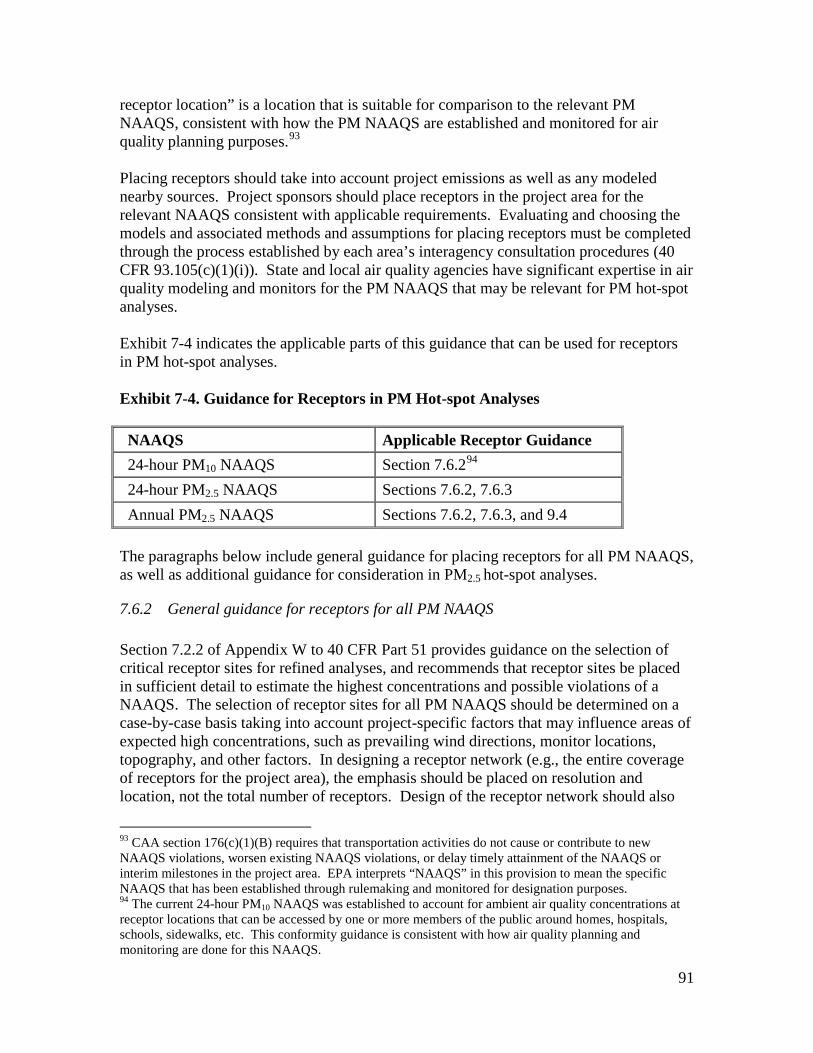
91

receptor location” is a location that is suitable for comparison to the relevant PM NAAQS, consistent with how the PM NAAQS are established and monitored for air quality planning purposes.93

Placing receptors should take into account project emissions as well as any modeled nearby sources. Project sponsors should place receptors in the project area for the relevant NAAQS consistent with applicable requirements. Evaluating and choosing the models and associated methods and assumptions for placing receptors must be completed through the process established by each area’s interagency consultation procedures (40 CFR 93.105(c)(1)(i)). State and local air quality agencies have significant expertise in air quality modeling and monitors for the PM NAAQS that may be relevant for PM hot-spot analyses. Exhibit 7-4 indicates the applicable parts of this guidance that can be used for receptors in PM hot-spot analyses. Exhibit 7-4. Guidance for Receptors in PM Hot-spot Analyses NAAQS Applicable Receptor Guidance 24-hour PM10 NAAQS Section 7.6.294 24-hour PM2.5 NAAQS Sections 7.6.2, 7.6.3 Annual PM2.5 NAAQS Sections 7.6.2, 7.6.3, and 9.4

The paragraphs below include general guidance for placing receptors for all PM NAAQS, as well as additional guidance for consideration in PM2.5 hot-spot analyses.

7.6.2 General guidance for receptors for all PM NAAQS Section 7.2.2 of Appendix W to 40 CFR Part 51 provides guidance on the selection of critical receptor sites for refined analyses, and recommends that receptor sites be placed in sufficient detail to estimate the highest concentrations and possible violations of a NAAQS. The selection of receptor sites for all PM NAAQS should be determined on a case-by-case basis taking into account project-specific factors that may influence areas of expected high concentrations, such as prevailing wind directions, monitor locations, topography, and other factors. In designing a receptor network (e.g., the entire coverage of receptors for the project area), the emphasis should be placed on resolution and location, not the total number of receptors. Design of the receptor network should also

93 CAA section 176(c)(1)(B) requires that transportation activities do not cause or contribute to new NAAQS violations, worsen existing NAAQS violations, or delay timely attainment of the NAAQS or interim milestones in the project area. EPA interprets “NAAQS” in this provision to mean the specific NAAQS that has been established through rulemaking and monitored for designation purposes. 94 The current 24-hour PM10 NAAQS was established to account for ambient air quality concentrations at receptor locations that can be accessed by one or more members of the public around homes, hospitals, schools, sidewalks, etc. This conformity guidance is consistent with how air quality planning and monitoring are done for this NAAQS.

92

consider whether any locations within the project area should be excluded from the modeling based on a location being restricted from public access or where a member of the public would normally be present only for a very short period of time. Examples include locations within a fenced property of a business, a median strip of a highway, a right-of-way on a limited access highway, or an approach to a tunnel. As described in Appendix W, air quality dispersion models are more reliable for estimating the magnitude of highest concentrations somewhere within a specified area and span of time than in predicting concentrations at a specific place and time. Therefore, receptors should be sited at all locations at which high concentrations may occur, rather than simply focusing on the expected worst case location. Receptor spacing in the vicinity of the source should be of sufficient resolution to capture the concentration gradients around the locations of maximum modeled concentrations. The majority of emissions from a highway or transit project will occur within several meters of the ground, and concentrations are likely to be greatest in proximity of near-ground sources. As such, receptors should be placed with finer spacing (e.g., 10-25 meters) closer to a near-ground source, and with wider spacing (e.g., 50-100 meters) farther from such a source. While prevailing wind directions may influence where maximum impacts are likely to occur, receptors should also be placed in all directions surrounding a project. It should not be assumed that the location of maximum concentration will always be located closest to the project itself. For example, if a highway project consists of a new bypass that branches off an existing highway with significant emissions, maximum concentrations may be expected at receptors farther from the project, but closer to the existing highway. Receptors should be sited as near as five meters from a source (e.g., the edge of a traffic lane or a source in a terminal), except possibly with projects involving urban street canyons where receptors may be appropriate within 2-10 meters of a project.95

In addition, if AERMOD is used to create a standardized receptor network (e.g., using AERMOD’s Cartesian or polar grid functions), receptors may inadvertently be placed within five meters of a project, and subsequently modeled. Such receptors should not be used when calculating design values in most cases.

Receptors should be placed to capture the impacts of the project and any nearby source that needs to be modeled. Receptor placement should be extended out to a sufficient distance from sources to account for emissions that affect concentrations throughout the project area, depending on the spatial extent of the project and the impacts of other modeled sources. EPA recommends that receptors should be sited to represent concentrations near-ground level, generally at a height of 1.8 meters above grade or less. Receptors should also be 95 See 40 CFR Part 58, Appendix D, Section 4.7.1(c)(1) and Appendix E, Section 6.3(b). The interagency consultation process should be used to determine when these provisions are relevant for a given analysis.

93

placed at higher elevations if needed to represent concentrations at several heights along multi-story buildings, such as apartment or office buildings. When completing air quality modeling for build and no-build scenarios, receptors should be placed in the same geographic locations in both scenarios so that direct comparisons can be made between the design values calculated at each receptor. Receptors are first determined based on the build scenario, and then placed in the same locations in the no-build scenario (when this scenario is modeled). See Section 9 for further information regarding calculating design values in a build/no-build analysis and appropriate receptors.

7.6.3 Additional guidance for receptors for the PM2.5 NAAQS There are additional considerations when placing receptors for the PM2.5 NAAQS, due to how this NAAQS was established. In the March 2006 final rule, EPA stated:

“Quantitative hot-spot analyses for conformity purposes would consider how projects of air quality concern are predicted to impact air quality at existing and potential PM2.5 monitor locations which are appropriate to allow the comparison of predicted PM2.5 concentrations to the current PM2.5 standards, based on PM2.5 monitor siting requirements (40 CFR Part 58).” (71 FR 12471)

EPA included this language in the preamble to the March 2006 final rule so that PM2.5 hot-spot analyses would be consistent with how the PM2.5 NAAQS were developed, monitored, and implemented. Receptors cannot be used for PM2.5 hot-spot analyses if they are at locations that would be inappropriate for ambient air quality monitoring for purposes of comparison to the NAAQS. In general, there are two factors in the PM2.5 monitoring regulations that need to be considered in determining the appropriateness of receptors for use in PM2.5 hot-spot analyses. First, a receptor must be “population-oriented” in order to be appropriate for comparison to either the 24-hour or annual PM2.5 NAAQS. Section 58.1 of the PM2.5 monitoring regulations defines population-oriented sites as:

“…residential areas, commercial areas, recreational areas, industrial areas where workers from more than one company are located, and other areas where a substantial number of people may spend a significant fraction of their day.”

Population-orientated receptors can be determined when receptors are placed for air quality modeling. In general, most locations, especially in urban areas, are population-oriented. Receptors placed near transportation projects, therefore, will most likely be population-oriented. Also, consideration should be given to the presence of people at locations around each receptor in determining whether the receptor is population-oriented, because the concentration predicted for the receptor can represent concentrations surrounding the receptor. Changes in the project area in the future analysis year should also be considered when placing receptors. For example, if a receptor is at a location that is currently not population-oriented, but a housing

94

development is planned for that location under the build and/or the no-build scenario, that receptor may be appropriate for comparison to the PM2.5 NAAQS. The second factor from the PM2.5 monitoring regulations is only relevant for the annual PM2.5 NAAQS. The PM2.5 monitoring regulations require that receptors for the annual PM2.5 NAAQS also represent “community-wide air quality.” Although receptors can be placed for the annual PM2.5 NAAQS prior to air quality modeling, further consideration is needed after air quality modeling to determine whether any of the modeled receptors are not appropriate for comparison to the annual PM2.5 NAAQS. See Section 9.4 of this guidance for how to determine appropriate receptor locations for the annual PM2.5 NAAQS.

7.7 RUNNING THE MODEL AND OBTAINING RESULTS After preparing all model inputs, the air quality model should be run to predict concentrations. Next, background concentrations need to be determined, as described in Section 8. Finally, the resulting concentrations at receptors should be combined with background concentrations from other sources to calculate design values, as described in Section 9. Note that, before the results of either AERMOD or CAL3QHCR are ready for use in calculating design values and determining conformity, the data will have to undergo some post-processing, depending on how the data was run in the models and the NAAQS being evaluated. See Appendix J for more details.

95

Section 8: Determining Background Concentrations from Nearby and Other Emission Sources

8.1 INTRODUCTION This section describes how to determine background concentrations for PM hot-spot analyses. Section 93.123(c)(1) of the conformity rule states that “estimated pollutant concentrations must be based on the total emissions burden which may result from the implementation of the project, summed together with future background concentrations….” Background concentrations do not include the emissions from the project itself.96

Instead, background concentrations for PM hot-spot analyses involve:

• Nearby sources: These are individual sources other than the highway or transit project that contribute to ambient concentrations in the project area. Some nearby sources may be included in the air quality modeling for PM hot-spot analyses, while other nearby sources can be reflected in representative background concentrations. In general, nearby sources would be included in air quality modeling only when those sources would be affected by the project; and

• Other sources: This term is intended to capture the background concentrations in the project area that are not from the project or any nearby sources that are modeled.

Further information is provided in Section 8.2 on when to include nearby sources in air quality modeling and in Section 8.3 on how to include the impact of other sources of emissions in a future analysis year. It is important to note that nearby sources may only be present for some PM hot-spot analyses. This section is consistent with EPA’s “Guideline on Air Quality Models” (Appendix W to 40 CFR Part 51), which provides the appropriate framework for defining the elements of background concentrations. Section 8.2.1 of Appendix W states that “background concentrations are an essential part of the total air quality concentration to be considered in determining source impacts.”97

Concentrations are expected to vary throughout a PM nonattainment or maintenance area, resulting from differences in emission sources, meteorology, terrain, and other factors. EPA believes that meeting Section 93.123(c)(1) requirements for PM hot-spot analyses will be different from what has occurred historically for CO hot-spot analyses, due to the fundamental differences between the contributors to PM and CO pollution and the projects that are required to have quantitative PM and CO hot-spot analyses. Additional information is provided in Section 8.3 of this guidance.

96 See Sections 4 through 6 for more information on how to estimate project emissions. 97 Section 8.2.3 recommends for “multi-source areas” that “two components of background should be determined: contributions from nearby sources and contributions from other sources.”

96

Evaluating and choosing the models and associated methods and assumptions for nearby sources and representative background concentrations must be completed through the process established by each area’s interagency consultation procedures (40 CFR 93.105(c)(1)(i)). State and local air quality agencies will have the primary expertise on what emission sources are expected to affect background concentrations, including any nearby sources. The state or local air agency is likely to have an understanding of the project area and knowledge about information needed to characterize background concentrations appropriately, due to experience in developing air quality demonstrations, emission inventories, and siting air quality monitors for a given NAAQS. The EPA Regional Office is also a key resource for discussions regarding the air quality monitoring network, SIP modeling, and other issues.

8.2 NEARBY SOURCES THAT REQUIRE MODELING Nearby sources are individual sources that contribute PM concentrations to the project area.98

In general, nearby sources need to be included in air quality modeling only when those sources would be affected by the project. An example of a project that could affect nearby sources would be a highway project whose primary purpose is to accommodate future growth in freight and goods movement; such a project could affect emissions from related activity at nearby marine ports, rail yards, or intermodal facilities. These types of nearby sources (that is, those affected by the project) need to be included in air quality modeling for the PM hot-spot analysis, as described in Section 7, because their emissions will change between build and no-build scenarios.

EPA anticipates that most PM hot-spot analyses will not involve modeling of nearby sources that are not affected by the project, such as a stationary source, since these types of nearby sources would typically be captured in the representative background concentrations described in Section 8.3. The following questions can be used by project sponsors, the relevant state or local air agency, the EPA Regional Office, and other members of the interagency consultation process to identify any nearby sources that are affected by the project:

• Are there any nearby sources in the project area? If no, then the remainder of Section 8.2 can be skipped.

• If yes, then: o Do these sources emit significant levels of emissions that could affect PM

concentrations in the project area? o Are emissions from any nearby sources expected to differ between the

build and no-build scenarios as a result of the project? 98 Section 8.2.3 of Appendix W describes “nearby sources” more generally as: “All sources expected to cause a significant concentration gradient in the vicinity of the source or sources under consideration for emission limit(s) should be explicitly modeled.”

97

EPA notes that there may be limited cases where nearby sources not affected by the project would also need to be included in the modeling for a PM hot-spot analysis. However, such cases would only occur when these sources are not captured in background concentrations for the project area. See Section 8.3 for further information on the factors used to determine representative background concentrations for these cases. For example, if a stationary source is located upwind of the project area, representative background concentrations should include concentrations from such a source whenever possible. As stated above, state and local air quality agencies and the EPA Regional Office are key resources in understanding how to characterize nearby sources in PM hot-spot analyses, including those nearby sources not affected by the project.

As discussed in Section 7.3, EPA recommends that AERMOD be used for any PM hot-spot analyses that involve nearby sources that need to be modeled. The air quality modeling for nearby sources that would be affected by the project must include any reasonably expected changes in operation of the nearby source between the build and no-build scenarios when both scenarios are necessary to demonstrate conformity. Refer to Section 7 for more information about using AERMOD, placing receptors, and other information for air quality modeling. Specific information on emissions from nearby sources should be obtained. The state and local air agency should be consulted on characterizing nearby sources. In addition, emission rates and other parameters of nearby sources should be consistent with any permits approved by the state or local air agency, when applicable. For unpermitted sources, emission information should be consistent with information used by air agencies for developing emission inventories for regulatory purposes. Sections 8.1 and 8.2 of Appendix W describe the information needed to characterize the emissions of nearby sources for air quality models. For the 24-hour PM2.5 and PM10 NAAQS, it is also important to consider Section 8.2.3 of Appendix W, which states that it is appropriate to “model nearby sources only during those times when they, by their nature, operate at the same time as the primary source(s) being modeled.” Finally, estimation of nearby source impacts may take into account the effectiveness of anticipated control measures in the SIP if they are already enforceable in the SIP.

8.3 OPTIONS FOR BACKGROUND CONCENTRATIONS PM hot-spot analyses should also include background concentrations from “other sources” as well as any nearby sources that are not included in modeling.99

99 Section 8.2.3 of Appendix W defines “contributions from other sources” as “that portion of the background attributable to all other sources (e.g., natural sources, minor sources and distant major sources)….”

There are several options provided below that meet the requirements of Section 93.123(c)(1) of the conformity rule that involve using representative air quality monitoring data. Whatever option is selected, the same background concentrations would be used at every receptor

98

used in the build and no-build scenarios for a PM hot-spot analysis. Additional options for background concentrations can be considered by the EPA Regional Office, OTAQ, and OAQPS. See Section 1.7 for contact information.

8.3.1 Using ambient monitoring data to estimate background concentrations Ambient monitoring data for PM10 and PM2.5 provide an important source of information to characterize the contributions from sources that affect the background concentrations in the project area, but are not captured by air quality modeling for the PM hot-spot analysis. Nonattainment and maintenance areas, and areas that surround them, have numerous sites for monitoring PM2.5 and PM10 concentrations that may be appropriate for estimating background concentrations.100 Project sponsors, relevant state or local air agencies, and the EPA Regional Office should identify the appropriate PM10 and PM2.5 monitoring data, along with information on each monitor’s site location, purpose, geographic scale, nearby land uses, and sampling frequency. EPA offers Air Explorer (based on Google Earth™ mapping software) as a user-friendly way to identify and visualize where monitoring sites are in operation and to obtain concentration data and descriptions of the site (such as the reported scale of spatial representation).101

The evaluation and selection of monitoring data for use in a particular analysis must follow the process defined in each area’s interagency consultation procedures. These discussions, as well as any maps or statistical techniques used to analyze background data, should be well-documented and included in the project-level conformity determination. Project sponsors should not use monitoring data for which EPA has granted data exclusion under the Exceptional Events rule (see 40 CFR 50.14). Using a Single Monitor Background concentration data should be as representative as possible for the project area examined by the PM hot-spot analysis.102

In most cases, the simplest approach will be to use data from the monitor closest to and upwind of the project area. However, all of the following factors need to be evaluated when considering monitors for use of their data as representative background concentrations:

100 Monitors in adjacent nonattainment, maintenance, and attainment areas should also be evaluated for use in establishing background concentrations, which may be appropriate if the air quality situation at those monitors can be determined to be reasonably similar to the situation in the project area. 101 Available online at: www.epa.gov/airexplorer/monitor_kml.htm. 102 In particular, there should be interagency consultation prior to using any ambient monitoring data set for PM2.5 that does not meet EPA requirements in Appendix N to 40 CFR Part 50 regarding data completeness, and any data set that reflects a sampling schedule that has been erratic or has resulted in more frequent samples in some seasons of a year than others. The guidance in Section 9 of this document assumes that the normal data completeness requirement (75% of scheduled samples in each calendar quarter of each year) has been met and that the monitoring data is evenly distributed across the year. Deviation from these conditions may make the steps given in Section 9 inappropriate.

http://www.epa.gov/airexplorer/monitor_kml.htm�

99

• Similar characteristics between the monitor location and project area: Monitors at locations that are similar to the project area should be preferred for this factor, whenever possible. If several monitors are available, preference should be given to the monitor with the most similar characteristics as the project area. Some questions to be considered include:

o Is the density and mix of emission sources around the monitor location similar to those around the project site?

o How well does the monitor capture the influence of nearby sources that are not affected by the project?

o Are there differences in land use or terrain between the two locations that could influence air quality in different ways?

o Is the monitor probe located at a similar height as the project (e.g., is the project at grade, but the monitor is on top of a high building)?

o What is the purpose of the monitor and what geographic scale of representation does the monitor have?

• Distance of monitor from the project area: Monitors closer to the project may have

concentrations most similar to the project area. If more than one such monitor is available, preference may be given to the closest representative monitor for this factor. There are some cases, however, where consideration of distance alone may mask the influence of other factors that need to also be considered (e.g., a monitor upwind of the project location may be preferred to an even closer monitor located downwind of the project).

• Wind patterns between the monitor and the project area: Monitors that are located in

directions that are frequently upwind of a project are more likely to represent a project area’s background concentrations than monitors that are frequently downwind.103

Preference should be given to upwind monitors for this factor, whenever appropriate.

The factors considered when selecting a particular monitor to represent background concentrations should be documented as part of the PM hot-spot analysis. Interpolating Between Several Monitors If, during interagency consultation, agencies conclude that no single ambient monitor is sufficiently representative of the project area, interpolating the data of several monitors surrounding the project area is also an option. The advantage of interpolation is that no single monitor is used exclusively in representing air quality for a project area. There may be projects sited in locations between large emission sources and areas several miles away with relatively low emissions, suggesting a gradient in concentrations across the nonattainment or maintenance area. If there are no monitors within or near the project 103 Constructing a “wind rose” (a graph that depicts the frequency of wind blowing from different directions) can be a useful tool in examining the frequency of wind blowing from different directions. EPA’s SCRAM website contains two programs for calculating wind statistics and wind roses, WINDROSE and WRPLOT.

100

area, then background concentrations from other sources may be difficult to estimate. Interpolation is an approach that allows estimates of background concentrations for a project to take advantage of monitoring data from multiple monitoring sites. Any planned interpolation methods must be addressed through the interagency consultation process. There are several approaches to interpolation that can be used. One simple method is weighted averaging, which places greater weight on nearby monitors and uses the inverse distance between the project site and the monitor to weight each monitor. For example, suppose monitors A, B, and C surround an unmonitored location, at distances 5, 10, and 15 miles from the site, respectively, the weighting of data from monitor A:

55.0151

101

51

51)( =

++=AWeight

The weighting for monitor B:

27.0151

101

51

101)( =

++=BWeight

The weighting for monitor C:

18.0151

101

51

151)( =

++=CWeight

If concentrations at A, B, and C are 10.0, 20.0, and 30.0 µg/m3, respectively, then the predicted concentration at the unmonitored site is 16.3 µg/m3. In most situations, the inverse-distance weighted average will provide a reasonable approximation of background concentrations due to other sources. Another interpolation approach is the inverse-squared distance weighting that weights monitors based on how close they are to the project (1/distance squared). Other, more advanced statistical methods to interpolate monitoring data may also be used, but these require significant geostatistical expertise.104

104 EPA’s MATS (

www.epa.gov/ttn/scram/modelingapps_mats.htm) and BenMAP (www.epa.gov/air/benmap) models incorporate another interpolation-based approach (Voronoi Neighbor Averaging). Consult those models’ documentation for further information.

http://www.epa.gov/ttn/scram/modelingapps_mats.htm�

http://www.epa.gov/air/benmap�

101

8.3.2 Adjusting air quality monitoring data to account for future changes in air quality: using chemical transport models

Options Using Chemical Transport Models (CTMs) To account for future emission changes, it may be appropriate in some cases to use future background concentrations that have been calculated based on modeled outputs from a CTM. CTMs are photochemistry models that are routinely used in regulatory analyses, including attainment demonstrations for PM SIPs and EPA regulatory analyses to support national or regional final rules. 105

In these types of analyses, CTM modeling is completed for a base and future year, and then these resulting PM concentrations are used to develop relative response factors (RRFs). These factors are then used to adjust the air quality monitoring data from the base year of the SIP or EPA final rule modeling. The end result will be predicted PM concentrations for monitoring locations for a future year (e.g., the attainment year addressed in the SIP).

Although project sponsors are not expected to operate CTMs, there may be available information from CTM modeling to support PM hot-spot analyses. There are two CTM-based options that may be available for PM hot-spot analyses:

1. Use existing pre-calculated future year PM concentrations from EPA or state or local air quality agency modeling. If available, the future year concentrations at a monitor used in the SIP or EPA rulemaking can be used for a PM hot-spot analysis, if the monitor is representative of the project area. Typically, projected annual average and/or 24-hour average PM design values for a future year will be available for monitoring site locations that are part of such modeling demonstrations.

2. In some cases, site-specific, post-processed concentrations may not be readily

available from states or EPA. Depending on the nature of the modeling, it may be possible to obtain CTM outputs that can be used to derive background concentrations.106

This may be an option if the standard post-processed data includes only a subset of monitoring sites in the domain or a subset of averaging times (e.g., annual average results are available, but not 24-hour average results).

Details on the recommended procedures for projecting PM2.5 concentrations using CTMs are contained in EPA’s “Guidance on the Use of Models and Other Analyses for Demonstrating Attainment of Air Quality Goals for Ozone, PM2.5, and Regional

105 Examples of commonly employed CTMs are shown on the SCRAM website at: www.epa.gov/scram001/photochemicalindex.htm. 106 Many CTM applications are post-processed with EPA’s MATS program available at: www.epa.gov/ttn/scram/modelingapps_mats.htm . MATS produces future year annual and quarterly PM2.5 outputs for both the annual and 24-hour PM2.5 NAAQS. The quarterly concentration information may not be routinely documented.

http://www.epa.gov/scram001/photochemicalindex.htm�

http://www.epa.gov/ttn/scram/modelingapps_mats.htm�

102

Haze.”107

The location where CTM modeling is completed, the location of the project, and determining representative monitors are important considerations in using CTM-based options for PM hot-spot analyses. Evaluating and choosing the models and associated methods and assumptions for using CTM-based options must be determined through interagency consultation (40 CFR 93.105(c)(1)(i)). The EPA Regional Office should consult with OTAQ and OAQPS in applying the above options or considering other options.

Additional Information and Considerations about CTMs EPA’s photochemical modeling guidance recommends using CTM outputs in a relative sense. Therefore the absolute predictions of a CTM in a future analysis year are not used to predict future background concentrations directly. Instead, appropriate future year design values or concentrations are derived from monitoring data that have been adjusted using the modeled relative change in PM concentrations. RRFs are calculated from the outputs of current (base) year and future year CTM results. These RRFs reflect the relative changes in concentrations between current and future years.108

An RRF is generally calculated as:

CTMby predicted year, basein ionsConcentratCTMby predicted year, futurein ionsConcentrat=RRF

Future year concentrations are then calculated by multiplying base year monitoring data by modeled RRFs, as follows: Base year measured concentration * RRF = Future year concentration Additionally, when using the CTM-based options, several criteria should be met:

• The CTM has demonstrated acceptable performance for the project area using

standard indicators of model performance.109

• The results of CTM runs are appropriate for the project and future analysis year(s) covered by the PM hot-spot analysis (e.g., the CTM modeling includes the project area and the modeling was completed for the analysis year or a year earlier than the analysis year).

• Any future emission reductions for sources within the CTM modeling demonstration are based on enforceable commitments in the SIP and/or are consistent with the conformity rule’s latest planning assumptions requirements (40 CFR 93.110).

107 See guidance for further information at: www.epa.gov/scram001/guidance/guide/final-03-pm-rh-guidance.pdf. 108 Future year concentrations of PM2.5 are calculated based on PM2.5 species concentrations that have been projected using RRFs for individual PM2.5 species. 109 Details on model performance evaluation and examples of model evaluation statistics may be found in Chapter 18 and Appendix A of the document “Guidance on the Use of Models and Other Analyses for Demonstrating Attainment of Air Quality Goals for Ozone, PM2.5, and Regional Haze,” referenced above.

http://www.epa.gov/scram001/guidance/guide/final-03-pm-rh-guidance.pdf�

http://www.epa.gov/scram001/guidance/guide/final-03-pm-rh-guidance.pdf�

103

• EPA or state modeling which includes future emissions reductions from a proposed rule or hypothetical emissions reductions that are not associated with enforceable SIP commitments or state or Federal rules should not be used.

• Any future emission reductions for sources within the CTM modeling demonstration should take effect prior to the year(s) for which the PM hot-spot analysis is conducted.

The PM hot-spot analysis year(s) will often be after a year for which CTM modeling is performed. In this case, the future background concentration for the analysis year should be the same year for which CTM modeling was performed. It is not technically justified to extrapolate background concentrations beyond the year in which data are available for the CTM modeling. For example, if future background concentrations were estimated based on CTM modeling for the year 2014, and the PM hot-spot analysis year was 2016, then the 2014 background estimate could be used for 2016. A project sponsor could not make a further adjustment based on an extrapolation to the year 2016; such an extrapolation would not be based on credible modeling or mathematical practices. Similarly, emissions-based “roll-back” and “roll-forward” techniques for adjusting current air quality monitoring data for future background concentrations are also not technically supported and would not allow projects sponsors to meet Section 93.123(c)(1) requirements. Note that in some cases, CTM adjusted background predictions for a future year may already incorporate emissions from the project’s no-build scenario (e.g., if the monitor used in the SIP modeling demonstration included emissions from the current project area). Adding modeled concentrations for the build scenario to this value would be essentially adding build emissions to the no-build emissions already accounted for in the background. In these cases, an adjustment may be appropriate only when comparing the build scenario to the NAAQS. In such cases, to evaluate predicted concentrations in the build scenario, the difference between modeled concentrations at each receptor in the build and no-build scenarios should be calculated as:

scenario build no i,receptor scenario build i,receptor ireceptor ionConcentrationConcentratDifference −= The result – the difference between the build and no-build scenarios at each receptor – should be added to background concentrations when calculating design values for the build scenario. Comparing a build scenario to the no-build scenario to demonstrate conformity will not involve any similar adjustments, since the same background concentrations are used in the build and no-build scenarios. Using this approach, only the changes in receptor concentrations affected by emission changes from the project or modeled nearby sources used in calculating design values. Evaluating and choosing the models and associated methods and assumptions for using these adjustments must be determined through interagency consultation (40 CFR 93.105(c)(1)(i)).

104

8.3.3 Adjusting air quality monitoring data to account for future changes in air quality: using an on-road mobile source adjustment factor

There may be limited cases in PM10 nonattainment or maintenance areas where it would be appropriate to adjust representative air quality monitoring data by the factor described in Section 93.123(c)(2) of the conformity rule. This provision states that “…the future background concentration should be estimated by multiplying current background by the ratio of future to current traffic and the ratio of future to current emission factors.” This method has been a credible option for CO hot-spot analyses. Since CO air quality problems are primarily due to on-road CO emissions, such a ratio is appropriate for CO hot-spot analyses. EPA has determined that this method may also be a credible option when on-road mobile sources overwhelm overall PM10 SIP inventories. Such a case could occur in a limited number of PM10 areas where on-road mobile emissions for directly emitted PM10 represent most of the overall directly emitted PM10 emission inventory (e.g., are 75% or more of the overall inventory).110

Such cases include smaller PM10 areas where paved and unpaved road dust are the main source of direct PM10 emissions. EPA notes that this option would increase background concentrations (as compared to options discussed in Section 8.3.1), in cases where road dust and VMT are expected to increase in the future. The EPA Regional Office should be consulted on a case-by-case basis if Section 93.123(c)(2) is considered for a PM10 hot-spot analysis.

However, EPA has determined that the method described in Section 93.123(c)(2) is not required by the conformity rule and is not a technically viable option for estimating background concentrations in all PM2.5 hot-spot analyses and most PM10 hot-spot analyses. PM2.5 and PM10 nonattainment problems are typically more complex and result from many different types of emission sources, including emissions from on-road, non-road, stationary, and area sources. It would not be appropriate to adjust PM air quality monitoring data from all source types based on an on-road mobile source adjustment factor only, as has been done in CO hot-spot analyses. While the conformity rule requires CO hot-spot analyses for only the largest and most congested intersections in a given area (40 CFR 93.123(a)(2)), PM hot-spot analyses are required for more complex highway and transit projects that can also involve nearby sources (40 CFR 93.123(b)(1)). For all of the above reasons, using the same ratios in most PM hot-spot analyses would not allow project sponsors to meet Section 93.123(c)(1) requirements.

110 Precursor emissions inventories should not be considered in such a determination, since precursor emissions are not considered in hot-spot analyses.

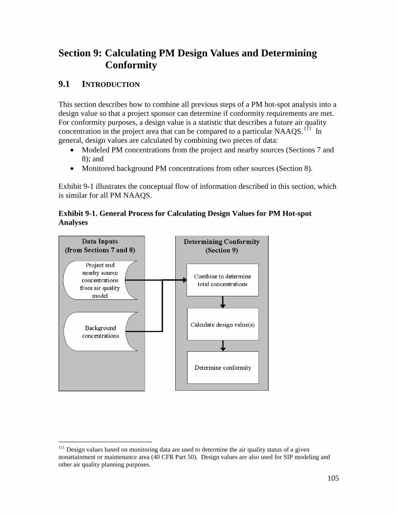
105

Section 9: Calculating PM Design Values and Determining Conformity

9.1 INTRODUCTION This section describes how to combine all previous steps of a PM hot-spot analysis into a design value so that a project sponsor can determine if conformity requirements are met. For conformity purposes, a design value is a statistic that describes a future air quality concentration in the project area that can be compared to a particular NAAQS.111

• Modeled PM concentrations from the project and nearby sources (Sections 7 and 8); and

In general, design values are calculated by combining two pieces of data:

• Monitored background PM concentrations from other sources (Section 8). Exhibit 9-1 illustrates the conceptual flow of information described in this section, which is similar for all PM NAAQS. Exhibit 9-1. General Process for Calculating Design Values for PM Hot-spot Analyses

111 Design values based on monitoring data are used to determine the air quality status of a given nonattainment or maintenance area (40 CFR Part 50). Design values are also used for SIP modeling and other air quality planning purposes.

106

This section describes how to calculate the specific statistical form of design values for each PM NAAQS and how to apply design values in build/no-build analyses for conformity purposes. This section also discusses how to determine which receptors for a particular project may or may not be appropriate for comparison to the annual PM2.5 NAAQS. This guidance is consistent with how design values are calculated for designations and other air quality planning purposes for each PM NAAQS. EPA is considering whether spreadsheet tools can be developed to assist state and local agencies in calculating design values for PM hot-spot analyses. This guidance is written for current and future PM2.5 and PM10 NAAQS. EPA will re-evaluate the applicability of this guidance as needed, if different PM NAAQS are promulgated in the future. The interagency consultation process must be used to determine the models, methods, and assumptions used for PM hot-spot analyses, including those used in calculating design values and completing build/no-build analyses (40 CFR 93.105(c)(1)(i)). State and local air quality agencies and EPA have significant expertise in air quality planning that may be useful resources for the topics covered by this section. Project sponsors should document the data and other details used for calculating design values for the build and no-build scenarios for a project-level conformity determination, as well as how appropriate receptors were determined.

9.2 USING DESIGN VALUES IN BUILD/NO-BUILD ANALYSES Design values are a fundamental component of PM hot-spot analyses, as they are the values compared to the NAAQS and between build and no-build scenarios. In general, a hot-spot analysis compares air quality concentrations with the proposed project (the build scenario) to air quality concentrations without the project (the no-build scenario). The conformity rule requires that the build scenario not cause or contribute to any new violations of the NAAQS, increase the frequency or severity of existing violations, or delay timely attainment as compared to the no-build scenario (40 CFR 93.116(a) and 93.123(c)(1)). Exhibit 9-2 (following page) illustrates the build/no-build analysis approach suggested in Section 2.4.

107

Exhibit 9-2. General Process for Using Design Values in Build/No-build Analyses

In general, project sponsors could begin by determining the design value for only one receptor in the build scenario: the receptor with the highest modeled air quality concentration, as described in Section 9.3. If the design value for this receptor is less than or equal to the relevant NAAQS, it can be assumed that conformity requirements are met at all receptors in the project area, without further analysis. If this is not the case, the project sponsor could choose to add mitigation or control measures and then determine if the new build scenario concentrations at the receptor with the highest modeled concentrations is less than or equal to the relevant NAAQS. If this is not the case, the project sponsor would calculate the design values at all receptors in the build scenario and also model the no-build scenario. Design values should then be calculated for the no-build scenario at all receptors with design values that exceeded the NAAQS in the build scenario. Conformity requirements are met if the design value for every appropriate receptor in the build scenario is less than or equal to the same receptor in the no-build scenario.112

112 This would be the receptor at the same geographic location in the build and no-build scenarios.

If not, then the project does not meet conformity requirements without

108

further mitigation or control measures to address air quality concentrations at such receptors, except in certain cases described below.113

A build/no-build analysis is typically based on design value comparisons done on a receptor-by-receptor basis. However, there may also be cases where a possible “new” violation at one receptor (in the build scenario) is relocated from a different receptor (in the no-build scenario). It would be necessary to calculate the design values for all receptors in the build and no-build scenarios to determine whether a “new” violation is actually a relocated violation. EPA addressed this issue in the preamble to the November 24, 1993 transportation conformity rule (58 FR 62213), where a “new” violation within the same intersection could be considered a relocated violation. Since 1993, EPA has made this interpretation only in limited cases with CO hot-spot analyses where there is a clear relationship between such changes (e.g., a reduced CO NAAQS violation is relocated from one corner of an intersection to another due to traffic-related changes from an expanded intersection). Any potential relocated violations in PM hot-spot analyses should be determined through the process established by each area’s interagency consultation procedures. When completing air quality modeling for build and no-build scenarios, receptors should be placed in identical locations so that direct comparisons can be made between design values calculated at receptors under each scenario. Also, design values are compared to the relevant NAAQS and between build and no-build scenarios after rounding has been done, which occurs in the final steps of design value calculations.114

Further details on rounding conventions for different PM NAAQS are included in Section 9.3 below.

Determining whether receptors are appropriate for the annual PM2.5 NAAQS would be done after air quality modeling is completed and design values are calculated, as described further in Section 9.4.

113 Additional mitigation or control measures can be considered at any point in the hot-spot analysis process. When such measures are considered, additional emissions and air quality modeling would need to be completed and new design values calculated to ensure that conformity requirements are met. 114 For example, conformity requirements would be met at a receptor if the final build design value is no greater than the final no-build design value, even if the pre-rounding build design value is greater than the pre-rounding no-build design value.

109

9.3 CALCULATING DESIGN VALUES AND DETERMINING CONFORMITY FOR PM HOT-SPOT ANALYSES

9.3.1 General As noted above, this conformity guidance is generally consistent with how design values are calculated for air quality monitoring and other EPA regulatory programs.115

Further details are included below about how design values should be calculated at receptors for build/no-build analyses, and examples of each design value calculation can be found in Appendix K of this guidance. These details and examples are primarily narrative in nature. EPA has also provided mathematical formulas of design values in Appendix K, which may be helpful for certain users.

9.3.2 Annual PM2.5 NAAQS Design Value The annual PM2.5 design value is currently defined as the average of three consecutive years’ annual averages, each estimated using equally-weighted quarterly averages.116

This NAAQS is met when the three-year average concentration is less than or equal to the annual PM2.5 NAAQS (currently 15.0 µg/m3):

Annual PM2.5 design value = ([Y1] average + [Y2] average + [Y3] average) ÷ 3

Where: [Y1] = Average annual PM2.5 concentration for the first year of air quality

monitoring data [Y2] = Average annual PM2.5 concentration for the second year of air quality

monitoring data [Y3] = Average annual PM2.5 concentration for the third year of air quality

monitoring data

The annual PM2.5 NAAQS is rounded to the nearest tenth of a µg/m3. For example, 15.049 rounds to 15.0, and 15.050 rounds to 15.1.117

115 EPA notes that design value calculations for PM hot-spot analyses involve using air quality modeling results based on either one year of site-specific measured meteorological data or five years of off-site measured meteorological data, rather than three years.

These rounding conventions should be followed when calculating design values for this NAAQS.

116 The design value for the annual PM2.5 NAAQS is defined for air quality monitoring purposes in 40 CFR Part 50.13. 117 A sufficient number of decimal places (3-4) should be retained during intermediate calculations for design values, so that there is no possibility of intermediate rounding or truncation affecting the final result. Rounding to the tenths place should only occur during final design value calculations, pursuant to Appendix N to 40 CFR Part 50.

110

Necessary Data This design value calculation assumes the project sponsor already has the following data in hand:

• Air quality modeling results: Average annual concentrations from the project and any nearby sources should be calculated from the air quality model output files.118

• Air quality monitoring data: 12 quarters of background concentration measurements (four quarters for each of three consecutive years). See Section 8 for more details on determining representative monitored background concentrations that meet all applicable monitoring requirements (such as data completeness).

The methodology for post-processing the air quality model output files will vary depending on what air quality model is used. Refer to Appendix J for details on preparing air quality model outputs for use in design value calculations.

119

Calculating Design Values and Determining Conformity Exhibit 9-3 (following page) illustrates how a design value is to be calculated and conformity determined for the annual PM2.5 NAAQS. This exhibit assumes that the project sponsor would first compare the receptor with the highest average annual concentration in the build scenario to the NAAQS to determine conformity. If conformity is not met at this receptor, design values would be calculated at all receptors in the build scenario. For any receptors with design values above the NAAQS in the build scenario, the project sponsor would then model the no-build scenario and calculate design values to determine if conformity requirements are met. An example of how to calculate design values for the annual PM2.5 NAAQS using this procedure is included in Appendix K. The steps below can also be described mathematically using the formulas found in Equation Set 1 in Appendix K. The steps shown in Exhibit 9-3 are described below. The initial step is to compare the build scenario to the NAAQS to see if the project conforms:

• Step 1. For each receptor, calculate the average annual concentrations with the air quality modeling results for each quarter and year of meteorological data used. If using AERMOD, the model does this step for you and provides the average annual concentrations as output; proceed to Step 2. If using CAL3QHCR, for each year of meteorological data, first determine the average concentration in each quarter. Then, within each year of meteorological data, add the average concentrations of all four quarters and divide by four to calculate the average annual modeled concentration for each year of meteorological data. Sum the modeled average annual concentrations from each year of meteorological data, and divide by the number of years of meteorological data used.

118 See Section 7.5.3 for further information on the number of years of meteorological data used in air quality modeling. For most PM hot-spot analyses, five years of meteorological data will be used. 119 The interagency consultation process should be used when situations require incorporation of any CTM results into design value calculations.

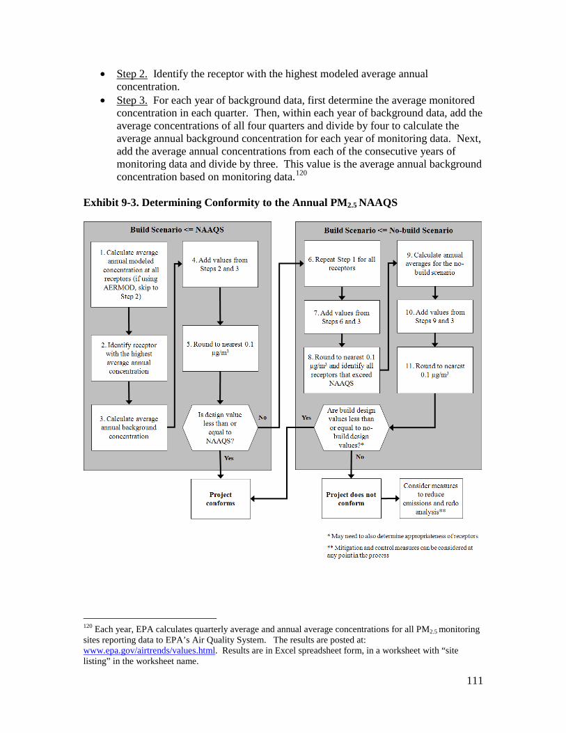
111

• Step 2. Identify the receptor with the highest modeled average annual concentration.

• Step 3. For each year of background data, first determine the average monitored concentration in each quarter. Then, within each year of background data, add the average concentrations of all four quarters and divide by four to calculate the average annual background concentration for each year of monitoring data. Next, add the average annual concentrations from each of the consecutive years of monitoring data and divide by three. This value is the average annual background concentration based on monitoring data.120

Exhibit 9-3. Determining Conformity to the Annual PM2.5 NAAQS

120 Each year, EPA calculates quarterly average and annual average concentrations for all PM2.5 monitoring sites reporting data to EPA’s Air Quality System. The results are posted at: www.epa.gov/airtrends/values.html. Results are in Excel spreadsheet form, in a worksheet with “site listing” in the worksheet name.

http://www.epa.gov/airtrends/values.html�

112

• Step 4. Add the average annual background concentration (from Step 3) to the average annual modeled concentration at the highest receptor (from Step 2) to determine the total average annual background concentration at this receptor.

• Step 5. Round to the nearest 0.1 µg/m3. This result is the annual PM2.5 design value at the highest receptor in the build scenario.

The project sponsor should then compare the design value from Step 5 to the annual PM2.5 NAAQS (currently 15.0 µg/m3). If the value is less than or equal to the NAAQS, the project conforms. If the design value is greater than the NAAQS, the project sponsor should then continue to Step 6:

• Step 6. Repeat the calculations described in Step 1 to determine average annual concentrations for all receptors in the build scenario.

• Step 7. Add the average annual modeled concentrations (from Step 6) to the average annual background concentrations (from Step 3).121

• Step 8. Round to the nearest 0.1 µg/m3. At each receptor, this value is the annual PM2.5 design value for the build scenario. Identify all receptors that exceed the annual PM2.5 NAAQS.

The result will be the total average annual concentration at each receptor in the build scenario.

• Step 9. From the no-build air quality modeling results, calculate the average annual concentrations at each receptor identified in Step 8.

• Step 10. For the no-build scenario, add the average annual modeled concentrations for the no-build scenario (from Step 9) to the average annual background concentrations (from Step 3). The result will be the total average annual concentration for each receptor identified in Step 8 under the no-build scenario.

• Step 11. Round to the nearest 0.1 µg/m3. This result is the annual PM2.5 design value for each receptor identified in Step 8 under the no-build scenario.

For each receptor with a design value that exceeded the NAAQS in the build scenario, compare the build design value (Step 8) to the no-build design value (Step 11). For the project to conform, the build design value must be less than or equal to the no-build design value at each receptor in the build scenario that exceeded the NAAQS (Step 8). If this is not the case, it may be necessary to determine if any receptors are not appropriate for conformity purposes (see Section 9.4).122

If a build scenario design value is greater than the no-build design value at any appropriate receptor, the sponsor should then consider additional mitigation and control measures, and revise the PM hot-spot analysis accordingly. Mitigation and control 121 As discussed in Section 8, the same air quality monitoring concentrations would not be expected to change between the build and no-build scenarios. As a result, the same background concentrations would be used for every receptor in the build and no-build scenario. 122 Project sponsors could decide to determine appropriate receptors for this NAAQS at Step 8, for any receptors where a NAAQS violation is predicted to occur. Also, in certain cases, project sponsors can also decide to calculate the design values for all receptors in the build and no-build scenarios and use the interagency consultation process to determine whether a “new” violation has been relocated (see Section 9.2).

113

measures could also be considered at any other point in the analysis before the project-level conformity determination is made. Refer to Section 10 for a discussion of potential measures.

9.3.3 24-hour PM2.5 NAAQS Design Value The 24-hour PM2.5 design value is currently defined as the average of three consecutive years’ 98th percentile concentrations of 24-hour values for each of those years.123 The NAAQS is met when that three-year average concentration is less than or equal to the currently applicable 24-hour PM2.5 NAAQS for a given area’s nonattainment designation (currently 35 µg/m3 for nonattainment areas for the 2006 PM2.5 NAAQS and 65 µg/m3 for nonattainment areas for the 1997 PM2.5 NAAQS).124

The design value for comparison to any 24-hour PM2.5 NAAQS is rounded to the nearest 1 µg/m3 (decimals 0.5 and greater are rounded up to the nearest whole number; decimals lower than 0.5 are rounded down to the nearest whole number). For example, 35.499 rounds to 35 µg/m3, while 35.500 rounds to 36.125


There are two analysis options, or tiers, that are available to project sponsors to estimate a 24-hour PM2.5 design value.126 Project sponsors can start with either the first or second tier analysis, since either tier is a viable approach for meeting conformity requirements. There may be cases where a project sponsor may decide to start with a first tier analysis, which is a conservative but less intensive approach.127

123 The design value for the 24-hour PM2.5 NAAQS is defined for air quality monitoring purposes in 40 CFR Part 50.13.

In other cases, project sponsors may decide to go directly to a second tier analysis. For example, depending on how the air quality model was run and its data post-processed, the actions needed to identify the highest modeled 24-hour concentration by quarter for a second tier analysis may not involve much additional time or effort, in which case the second tier approach may be

124 There are only two areas where conformity currently applies for both the 1997 and 2006 24-hour PM2.5 NAAQS. While both 24-hour NAAQS must be considered in these areas, in practice if the more stringent 2006 24-hour PM2.5 NAAQS is met, then the 1997 24-hour PM2.5 NAAQS is met as well. 125 A sufficient number of decimal places (3-4) should be retained during intermediate calculations for design values, so that there is no possibility of intermediate rounding or truncation affecting the final result. Rounding should only occur during final design value calculations, pursuant to Appendix N to 40 CFR Part 50. 126 This approach is consistent with EPA’s approach for calculating design values for other EPA regulatory programs. See the EPA March 23, 2010 memorandum from Stephen D. Page at www.epa.gov/scram001/Official%20Signed%20Modeling%20Proc%20for%20Demo%20Compli%20w%20PM2.5.pdf. 127 While less data intensive and therefore possibly quicker to execute, the first tier approach is considered more conservative as compared to the second tier analysis. The first tier approach assumes that the estimated highest predicted concentration attributable to the project and nearby sources will occur in the future on each of the days from which the three-year average 98th percentile background concentration is derived (which may not occur).

http://www.epa.gov/scram001/Official%20Signed%20Modeling%20Proc%20for%20Demo%20Compli%20w%20PM2.5.pdf�

http://www.epa.gov/scram001/Official%20Signed%20Modeling%20Proc%20for%20Demo%20Compli%20w%20PM2.5.pdf�

114

preferred from that start. Under either tier, the contributions from the project, any nearby sources, and background concentrations from other sources are combined for a given analysis year, as described further below. Examples of how to calculate design values for the 24-hour PM2.5 NAAQS using each tier are included in Appendix K. Necessary Data This design value calculation assumes the project sponsor already has the following data in hand:

• Air quality modeling results: The highest 24-hour average concentration from the project and any nearby sources should be calculated based on the air quality model output files, depending on what tier of analysis is used:

o In a first tier analysis, the highest 24-hour values from each year of meteorological data should be averaged together.

o In a second tier analysis, the highest 24-hour values from each quarter and year of meteorological data should be averaged together per quarter.

Post-processing the air quality model output files will vary depending on what air quality model is used in the hot-spot analysis. Refer to Appendix J for a discussion of air quality model output file formats.

• Air quality monitoring data: 12 quarters of background concentration measurements (four quarters for each of three consecutive years). See Section 8 for more details on determining representative monitored background concentrations that meet all applicable monitoring requirements (such as data completeness).128

Calculating Design Values and Determining Conformity Using a First Tier Analysis The first tier consists of directly adding the highest average modeled 24-hour concentrations to the average 98th percentile 24-hour background concentrations. Exhibit 9-4 (following page) illustrates how a design value would be calculated under a first tier analysis for a given receptor. The steps shown in Exhibit 9-4 are described in detail below, and are also described mathematically using the formulas found in Equation Set 2 in Appendix K.

128 The interagency consultation process should be used when situations require incorporation of any CTM results into design value calculations.

115

Exhibit 9-4. Determining Conformity to the 24-hour PM2.5 NAAQS Using First Tier Analysis

The initial step in a first tier analysis is to compare the build scenario to the NAAQS to see if the project conforms:

• Step 1. From the air quality modeling results from the build scenario, identify the receptor with the highest average 24-hour concentration. This is done by first separating the air quality model output into each year of meteorological data. Second, for each receptor and year of meteorological data, identify the 24-hour period (midnight-to-midnight) with the highest average concentration throughout the entire year. Finally, at each receptor, average the highest 24-hour concentrations from each year of meteorological data across all years. The receptor with the highest value is used to calculate the 24-hour PM2.5 design value.

• Step 2. Calculate the average 98th percentile 24-hour background concentration using the 98th percentile 24-hour concentrations of the three most recent years of air quality monitoring data. To calculate the 98th percentile background concentrations for each year of monitoring data, first count the number of 24-hour background measurements in each year. Next, order the highest eight monitoring values in each year from highest to lowest and rank each value from 1 (highest) to 8 (eighth highest). Consult Exhibit 9-5 (following page) to determine which of these eight values is the 98th percentile value. Using the results from the three

116

years of monitoring data, calculate the three-year average of the 98th percentile concentrations.129

• Step 3. Add the highest average 24-hour modeled concentration (Step 1) to the average 98th percentile 24-hour background concentration (Step 2) and round to the nearest 1 µg/m3. The result is the 24-hour PM2.5 design value at the highest receptor in the build scenario.

Exhibit 9-5. Ranking of 98th Percentile Background Concentration Values130

Number of Background

Concentration Values

Rank of Value Corresponding to

98th Percentile Concentration

1-50 1 51-100 2 101-150 3 151-200 4 201-250 5 251-300 6 301-350 7 351-366 8

If the design value calculated in Step 3 is less than or equal to the relevant 24-hour PM2.5 NAAQS, then the project conforms. If it is greater than the 24-hour PM2.5 NAAQS, conformity is not met, and the project sponsor has two options:

• Repeat the first tier analysis for the no-build scenario at all receptors that exceeded the NAAQS in the build scenario. If the calculated design value for the build scenario is less than or equal to the design value for the no-build scenario at all of these receptors, then the project conforms;131

• Conduct a second tier analysis as described below. or

129 Assuming a regular monitoring schedule and a resulting data set that meets the completeness requirements of 40 CFR Part 50 Appendix N, the result of Step 2 will be the design value for the monitoring site used to estimate the background concentrations. Each year, EPA calculates the 98th percentile concentration for each of the most recent three years and the average of the three current annual values for every PM2.5 monitor, based on the data reported to EPA’s Air Quality System. Project sponsors may use the EPA-calculated design values directly instead of executing Step 2, or may compare their result from Step 2 to the EPA-calculated design value. These design values appear in the worksheet “Site Listing” of the latest PM2.5 design value spreadsheet posted at: www.epa.gov/airtrends/values.html. 130 This exhibit is based on a table in Appendix N to 40 CFR Part 50, and ranks the 98th percentile of background concentrations pursuant to the total number of air quality monitoring measurements. 131 In certain cases, project sponsors can also decide to calculate the design values for all receptors in the build and no-build scenarios and use the interagency consultation process to determine whether a “new” violation has been relocated (see Section 9.2).

http://www.epa.gov/airtrends/values.html�

117

Calculating Design Values and Determining Conformity Using a Second Tier Analysis The second tier involves a greater degree of analysis, in that the highest modeled concentrations and the 98th percentile background concentrations are not added together for each receptor directly, as in a first tier analysis. Unlike a first tier analysis, which uses the average of the highest modeled 24-hour concentration from each year of meteorological data, a second tier analysis uses the average of the highest modeled 24-hour concentration within each quarter of each year of meteorological data. In other words, impacts from the project, nearby sources, and other background concentrations are calculated on a quarterly basis before determining the 98th percentile concentration resulting from these inputs. Exhibit 9-6 (following page) and the following steps provide details for calculating a design value for the 24-hour PM2.5 NAAQS under a second tier analysis. These steps can also be described mathematically using the formulas found in Equation Set 3 in Appendix K. A project sponsor would initially complete these steps for the build scenario; then, if necessary, repeat the steps for the no-build scenario. Steps 1 and 2 of a second tier analysis are completed only once for all receptors, since the same background concentrations would be used for every receptor in either the build or no-build scenario.

• Step 1. Count the number of measurements for each year of monitoring data used for background concentrations for other sources.

• Step 2. For each year of monitoring data used, determine the eight highest 24-hour background concentrations for each quarter modeled. For most hot-spot analyses for the 24-hour PM2.5 NAAQS, modeling would be completed for all four quarters of each analysis year. This would therefore result in 32 values (eight concentrations for four quarters) for each year of monitoring data.132, 133

The remaining steps are completed for calculating the 24-hour PM2.5 design value at each receptor:

• Step 3. At each receptor, identify the highest modeled 24-hour concentration in each quarter, averaged across each year of meteorological data used for air quality modeling.

• Step 4. At each receptor, add the highest modeled concentration in each quarter (from Step 3) to each of the eight highest 24-hour background concentrations for the same quarter for each year of monitoring data (from Step 2). At each receptor, this step will result in eight 24-hour concentrations in each of four quarters for a total of 32 values for each year of monitoring data.

132 Section 3.3.4 describes how the number of quarters modeled should be determined. In most PM hot-spot analyses for the 24-hour PM2.5 NAAQS, all four quarters of the analysis year will be modeled. There are limited cases where modeling only one quarter would be appropriate. 133 24-hour PM2.5 concentrations for any monitoring site reported to EPA’s Air Quality System can be obtained by using the data download tools available at: www.epa.gov/airexplorer/monitor_kml.htm.


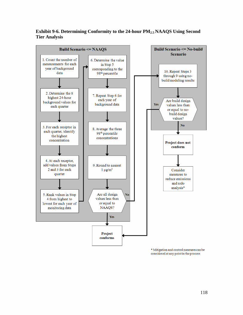
118

Exhibit 9-6. Determining Conformity to the 24-hour PM2.5 NAAQS Using Second Tier Analysis

119

• Step 5. For each receptor and year of monitoring data, order the 32 values from Step 4 from highest to lowest and rank each value from 1 (highest concentration) to 32 (lowest concentration).

• Step 6. Based on the number of background concentration values you have (from Step 1), use Exhibit 9-7 to determine which value in the column (from Step 5) represents the 98th percentile concentration for each receptor. For example, if you have 180 background concentration values in a year, Exhibit 9-7 shows that the 4th highest value would represent the 98th percentile. Take the value at each receptor that has this rank.

Exhibit 9-7. Ranking of 98th Percentile Background Concentration Values134

Number of Background

Concentration Values

Rank of Value Corresponding to

98th Percentile Concentration

1-50 1 51-100 2 101-150 3 151-200 4 201-250 5 251-300 6 301-350 7 351-366 8

• Step 7. Repeat Step 6 for each of the three years of background monitoring data.

The result will be three 24-hour 98th percentile concentrations at each receptor, one for each year of monitoring data.

• Step 8. At each receptor, calculate the average of the three 24-hour 98th percentile concentrations determined in Step 7.

• Step 9. Round the average concentrations from Step 8 to the nearest 1 µg/m3. At each receptor, this value is the 24-hour PM2.5 design value for the build scenario.

Compare the design values to the relevant 24-hour PM2.5 NAAQS. If the design values at all receptors are less than or equal to the NAAQS, then the project conforms. If this is not the case, proceed to Step 10:

• Step 10. Using modeling results for the no-build scenario, repeat Steps 3 through 9 for all receptors with a design value that exceeded the PM2.5 NAAQS in the build scenario. The result will be a 24-hour PM2.5 design value at such receptors for the no-build scenario.

134 This exhibit is based on a table in Appendix N to 40 CFR Part 50, and ranks the 98th percentile of background concentrations pursuant to the number of air quality monitoring measurements.

120

Compare the build design values (from Step 9) to the no-build design values (from Step 10), identifying which value is higher at each receptor. For the project to conform, the build design values must be less than or equal to the no-build design value for all of the receptors that exceeded the NAAQS in the build scenario.135

If the build scenario design value is greater than the no-build design value at any appropriate receptor, the project sponsor should then consider additional mitigation and control measures, and revise the PM hot-spot analysis accordingly. Mitigation and control measures could also be considered at any other point in the analysis before the project-level conformity determination is made. Refer to Section 10 for a discussion of potential measures.

9.3.4 24-hour PM10 NAAQS Design Value Compliance with the 24-hour PM10 NAAQS is based on the expected number of 24-hour exceedances of a particular level (currently 150 µg/m3), averaged over three consecutive years.136 Currently, the NAAQS is met when the expected number of exceedances is less than or equal to 1.0.137

The 24-hour PM10 NAAQS design value is rounded to the nearest 10 µg/m3. For example, 155.511 rounds to 160, and 154.999 rounds to 150.138


The contributions from the project, any nearby sources, and background concentrations from other sources are combined for a given analysis year, as described further below. Examples of how to calculate design values for the 24-hour PM10 NAAQS are included in Appendix K.

135 In certain cases, project sponsors can also decide to calculate the design values for all receptors in the build and no-build scenarios and use the interagency consultation process to determine whether a “new” violation has been relocated (see Section 9.2). 136 The 24-hour PM10 NAAQS and supporting technical documentation can be found in 40 CFR Part 50.6. 137 The term “expected” means that the actual number of observed exceedances is adjusted upwards when observations are missing for some days, to reflect the air quality statistically expected for those days. The design value for the 24-hour PM10 NAAQS is the next highest observed (monitored or modeled) concentration after the concentrations that could be above 150 µg/m3 without causing the expected number of exceedances to be greater than 1.0. 138 A sufficient number of decimal places (3-4) in modeling results should be retained during intermediate calculations for design values, so that there is no possibility of intermediate rounding or truncation affecting the final result. Rounding to the nearest 10 ug/m3 should only occur during final design value calculations, pursuant to Appendix K to 40 CFR Part 50. Monitoring values typically are reported with only one decimal place.

121

Necessary Data This design value calculation assumes the project sponsor already has the following data in hand:

• Air quality modeling results: In most PM hot-spot analyses, five years of meteorological data will be used to complete air quality modeling for the project and any nearby sources.139 In this case, the sixth-highest 24-hour modeled concentration should be calculated for each receptor.140

• Air quality monitoring data: 12 quarters of background concentration measurements (four quarters for each of three consecutive years). See Section 8 for more details on determining representative monitored background concentrations that meet all applicable monitoring requirements (such as data completeness).

Note that AERMOD can be configured to give you these values directly. CAL3QHCR output needs to be post-processed to obtain the sixth-highest value from five years of meteorological data. See more details below and refer to Appendix J for a discussion of air quality model output file formats.

141

Calculating Design Values and Determining Conformity The 24-hour PM10 design value is calculated at each receptor by directly adding the sixth-highest modeled 24-hour concentrations (if using five years of meteorological data) to the highest 24-hour background concentration (from three years of monitoring data). Exhibit 9-8 (following page) illustrates how a design value would be calculated. The steps shown in Exhibit 9-8 are described in detail below and are also described mathematically using the formulas found in Equation Set 4 in Appendix K. The initial step is to compare the build scenario to the NAAQS to see if the project conforms:

• Step 1. From the air quality modeling results for the build scenario, identify the sixth-highest 24-hour concentration for each receptor (across five years of meteorological data, in most cases). When using AERMOD, the model can be configured to produce these values.142

• Step 2. Identify the receptor with the highest sixth-highest 24-hour concentration. That is, compare the sixth-highest modeled concentrations (i.e., the concentrations

When using CAL3QHCR, output needs to be post-processed to obtain the sixth-highest values from five years of meteorological data.

139 Section 7.5.3 of this guidance provides further information on the number of years of meteorological data used in air quality modeling. 140 See description in Section 7.2.1.1 of Appendix W. Users with one year of site-specific meteorological data should select the 2nd highest 24-hour PM10 concentration. If using less than one year of meteorological data (such as one quarter), users should select the highest 24-hour concentration. 141 The interagency consultation process should be used when situations require incorporation of any CTM results into design value calculations. 142 For example, users could employ the RECTABLE keyword in the AERMOD output pathway. See Appendix J to this guidance for further information.

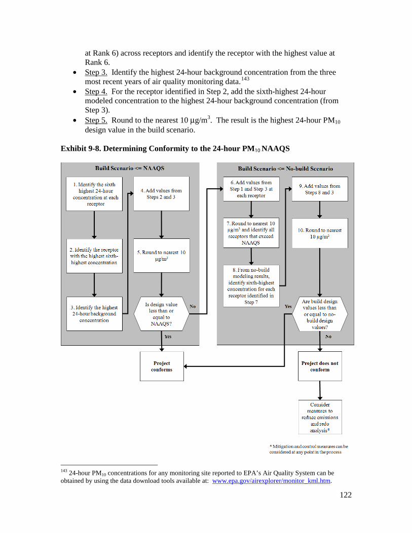
122

at Rank 6) across receptors and identify the receptor with the highest value at Rank 6.

• Step 3. Identify the highest 24-hour background concentration from the three most recent years of air quality monitoring data.143

• Step 4. For the receptor identified in Step 2, add the sixth-highest 24-hour modeled concentration to the highest 24-hour background concentration (from Step 3).

• Step 5. Round to the nearest 10 µg/m3. The result is the highest 24-hour PM10 design value in the build scenario.

Exhibit 9-8. Determining Conformity to the 24-hour PM10 NAAQS

143 24-hour PM10 concentrations for any monitoring site reported to EPA’s Air Quality System can be obtained by using the data download tools available at: www.epa.gov/airexplorer/monitor_kml.htm.


123

The project sponsor should then compare the design value from Step 5 to the 24-hour PM10 NAAQS (currently 150 µg/m3). If the design value calculated in Step 5 is less than or equal to the NAAQS, the project conforms. If the design value is greater than the NAAQS, the project sponsor should then continue to Step 6:

• Step 6. For each receptor in the build scenario, add the sixth-highest 24-hour modeled concentration (from Step 1) to the highest 24-hour background concentration from the three most recent years of air quality monitoring data (from Step 3).

• Step 7. Round to the nearest 10 µg/m3. At each receptor, this value is the 24-hour PM10 design value for the build scenario. Identify all receptors that exceed the 24-hour PM10 NAAQS.

• Step 8. From the no-build air quality modeling results, identify the sixth-highest 24-hour concentration for each receptor identified in Step 7.

• Step 9. Add the sixth-highest 24-hour modeled concentration in the no-build scenario (from Step 8) to the highest 24-hour background concentration from the three most recent years of air quality monitoring data (from Step 3).

• Step 10. Round to the nearest 10 µg/m3. The result is the 24-hour PM10 design value under the no-build scenario for each receptor identified in Step 7.

For each receptor with a design value that exceeded the NAAQS in the build scenario, compare the build design value (from Step 7) to the no-build design value (from Step 10). For the project to conform, the build design value must be less than or equal to the no-build design value at each receptor in the build scenario that exceeded the NAAQS (Step 7).144

If the build scenario design value is greater than the no-build design value at any appropriate receptor, the project sponsor should then consider additional mitigation and control measures, and revise the PM hot-spot analysis accordingly. Mitigation and control measures could also be considered at any other point in the analysis before the project-level conformity determination is made. Refer to Section 10 for a discussion of potential measures. More advanced methods of calculating a PM10 design value, such as combining modeled and monitored concentrations on a quarterly basis, may be considered on a case-by-case basis by the EPA Regional Office, OTAQ, and OAQPS. Any alternative methods for calculating PM10 design values must be evaluated and chosen through the process established by each area’s interagency consultation procedures (40 CFR 93.105(c)(1)(i)).

144 In certain cases, project sponsors can also decide to calculate the design values for all receptors in the build and no-build scenarios and use the interagency consultation process to determine whether a “new” violation has been relocated (see Section 9.2).

124

9.4 DETERMINING APPROPRIATE RECEPTORS FOR COMPARISON TO THE ANNUAL PM2.5 NAAQS

9.4.1 General When hot-spot analyses are done for the annual PM2.5 NAAQS, there is an additional step that may be necessary to determine whether a receptor is appropriate to compare to this NAAQS. In the March 2006 final rule, EPA stated:

“Quantitative hot-spot analyses for conformity purposes would consider how projects of air quality concern are predicted to impact air quality at existing and potential PM2.5 monitor locations which are appropriate to allow the comparison of predicted PM2.5 concentrations to the current PM2.5 standards, based on PM2.5 monitor siting requirements (40 CFR Part 58).” (71 FR 12471)

EPA included this language in the preamble to the March 2006 final rule so that PM2.5 hot-spot analyses would be consistent with how the PM2.5 NAAQS are developed, monitored, and implemented. Receptors cannot be used for PM2.5 hot-spot analyses if they are at locations that would not be appropriate for air quality monitoring purposes for the NAAQS. If conformity requirements are met at all receptors, it is unnecessary to determine whether receptors are appropriate for comparison to the annual PM2.5 NAAQS; in such a case, project sponsors can conclude that conformity requirements are met at all appropriate receptors. An “appropriate receptor location” under Section 93.123(c)(1) of the conformity rule is a location that is suitable for comparison to the relevant NAAQS, consistent with how the PM NAAQS are established and monitored for air quality planning purposes.145

9.4.2 Factors for determining appropriate receptors for comparison to the annual PM2.5 NAAQS

As discussed in Section 7.6, receptors can be placed prior to air quality modeling for all PM NAAQS. Furthermore, the appropriateness of receptor locations for the 24-hour PM2.5 NAAQS (and the 24-hour PM10 NAAQS) can be determined prior to air quality modeling. However, for the annual PM2.5 NAAQS, appropriate receptors should be determined after air quality modeling is completed, in order to be consistent with the PM2.5 monitoring regulations.146

145 See CAA Section 176(c)(1)(B). EPA interprets “NAAQS” in this provision to mean the specific NAAQS that has been established through rulemaking and monitored for designations purposes.

The paragraphs below provide additional guidance

146 As stated above, PM hot-spot analysis must be based on receptors that are appropriate for comparison to the annual PM2.5 NAAQS and consistent with the monitoring regulations for this NAAQS. EPA’s monitoring regulations allow for micro and middle scale sites to be compared to the annual PM2.5 NAAQS “where certain population-oriented micro scale or middle scale PM2.5 monitoring sites are determined by the Regional Administrator to collectively identify a larger region of localized high ambient PM2.5 concentrations” (40 CFR 58.30(a)). In order to determine if “a larger region of localized high ambient PM2.5 concentrations” is present in a given PM hot-spot analysis, it is critical to know which receptors have concentrations above the NAAQS and whether a significant number of similar receptors with high

125

when calculating design values and determining conformity for the annual PM2.5 NAAQS, through the steps described in Section 9.3.2. There are generally two factors in the PM2.5 monitoring regulations that need to be considered in determining the appropriateness of receptors for use in PM2.5 hot-spot analyses:

• Population-orientation: A receptor must be “population-oriented” in order to be appropriate for comparison to either the 24-hour or annual PM2.5 NAAQS.147

• Community-wide air quality: A receptor for the annual PM2.5 NAAQS must also represent “community-wide air quality”; this factor does not have to be satisfied for the 24-hour PM2.5 NAAQS.

This factor can be addressed when placing receptors prior to air quality modeling (see Section 7.6).

Section 9.3.2 includes an approach for conducting build/no-build analyses for the annual PM2.5 NAAQS, in which the appropriateness of receptors is determined only in cases where a design value in the build scenario is higher than the NAAQS and the design value in the no-build scenario. As noted above, if conformity requirements are met at all receptors, it is unnecessary to determine whether receptors are not appropriate for comparison to the annual PM2.5 NAAQS; in such a case, project sponsors can conclude that conformity requirements are met at all appropriate receptors. Evaluating and choosing the models and associated methods and assumptions, including appropriate receptor locations for the annual PM2.5 NAAQS, must be completed through the process established by each area’s interagency consultation procedures (40 CFR 93.105(c)(1)(i)). State and local air quality agencies and EPA have significant expertise in air quality planning and monitoring purposes that may be useful resources in determining appropriate receptor locations for the annual PM2.5 NAAQS. For example, under the PM2.5 monitoring regulations, the EPA Regional Offices determine whether micro or middle scale PM2.5 air quality monitors are eligible for comparison to the annual PM2.5 NAAQS, as discussed further below.

9.4.3 Overview of PM2.5 monitoring regulations The annual PM2.5 NAAQS was established to capture air quality concentrations over larger areas that represent “community-wide air quality.”148

concentrations represent a large portion of the project area. Such an assessment cannot be done qualitatively prior to air quality modeling.

Therefore, an appropriate receptor for hot-spot analyses for this NAAQS must also represent community-wide air quality. There are several parts of the PM2.5 monitoring regulations that describe how an existing or potential monitor location can represent community-wide air quality, and EPA will rely on this same information for determining appropriate receptor locations for

147 See 40 CFR 58.1. 148 The 1997 annual PM2.5 NAAQS was primarily based on health studies using neighborhood and larger scale air quality monitoring data (62 FR 38651-38760).

126

conformity purposes. Like ambient PM2.5 monitoring sites, not every receptor may be appropriate for comparing a predicted design value with the annual PM2.5 NAAQS. Air quality monitors that represent community-wide air quality and are compared to the annual PM2.5 NAAQS typically are of neighborhood and larger scales, as defined by the PM2.5 monitoring regulations. Section 4.7.1(b) of Appendix D to 40 CFR Part 58 states:

“The required monitoring stations or sites must be sited to represent community-wide air quality….These monitoring stations will typically be at neighborhood or urban scale.”

Therefore, conformity requirements must be met at any receptor that is at a location that would also be appropriate for an existing or potential neighborhood or larger scale air quality monitor for the annual PM2.5 NAAQS. In general, population-oriented receptors that are farther away from the project would be similar to potential neighborhood or larger scale monitoring sites and would be representative of community-wide air quality in all PM hot-spot analyses. The PM2.5 monitoring regulations also address when smaller scale locations are considered to represent community-wide air quality and can be compared to the annual PM2.5 NAAQS. Section 58.30(a) of the regulations states:

“(1) PM2.5 data that are representative, not of areawide but rather, of relatively unique population-oriented microscale, or localized hot-spot, or unique population-oriented middle-scale impact sites are only eligible for comparison to the 24-hour PM2.5 NAAQS; and (2) There are cases where certain population-oriented microscale or middle scale PM2.5 monitoring sites are determined by the Regional Administrator to collectively identify a larger region of localized high ambient PM2.5 concentrations. In those cases, data from these population-oriented sites would be eligible for comparison to the annual PM2.5 NAAQS.”149

Other parts of the PM2.5 monitoring regulations also address middle and microscale locations. Section 4.7.1(b) of Appendix D to 40 CFR Part 58 states:

“… in certain instances where population-oriented micro or middle scale PM2.5 monitoring are determined by the Regional Administrator to represent many such locations throughout a metropolitan area, these smaller scales can be considered to represent community-wide air quality.”

149 Thus, unless the Regional Administrator has made this finding after a case-by-case evaluation, a population-oriented microscale or middle scale monitoring site (including one located near malls, neighborhoods, schools, etc.) cannot be presumed to represent community-wide air quality.

127

Section 4.7.1(c)(1) and (2) note that sites very close to individual sources, such as traffic corridors in urban areas, may be appropriate sites for locating PM2.5 monitors that represent community-wide air quality:

“In some circumstances, the microscale is appropriate for particulate sites; community-oriented…sites measured at the microscale level should, however, be limited to urban sites that are representative of long-term human exposure and of many such microenvironments in the area.

In many situations, monitoring sites that are representative of microscale or middle-scale impacts are not unique and are representative of many similar situations. This can occur along traffic corridors or other locations in a residential district. In this case, one location is representative of a number of small scale sites and is appropriate for evaluation of long-term or chronic effects.”

In general, receptors that are closer to a project would be similar to potential micro and middle scale air quality monitoring sites and would be appropriate for comparison to the annual PM2.5 NAAQS if they represent community-wide air quality.150

9.4.4 Conformity guidance for all projects in annual PM2.5 NAAQS areas

Receptors at Neighborhood or Larger Scale Locations As described above, all population-oriented receptors at locations where a neighborhood or larger scale monitor could be located are appropriate for comparison to the annual PM2.5 NAAQS in a PM2.5 hot-spot analysis. In general, receptors farther away from any transportation project (e.g., 100 meters or more away from a larger highway project) would represent neighborhood scale locations under the PM2.5 monitoring regulations.151

The PM2.5 monitoring regulations do not provide further specific information for determining neighborhood or larger scale locations for PM hot-spot analyses. However, Figure E-1 in Appendix E of 40 CFR Part 58 specifies distances from a roadside where monitors of different scales may be located relative to a highway or intersection. See Section 9.4.5 for further information on when a receptor represents neighborhood and larger scale locations for these types of projects.

Receptors at Micro or Middle Scale Locations As described above, population-oriented receptors that are at locations where a micro or middle scale monitor could be located are appropriate for comparison to the annual PM2.5 NAAQS, if they represent community-wide air quality. In general, a receptor or 150 PM2.5 data from population-oriented microscale or middle scale monitoring sites (including those located near malls, neighborhoods, schools, etc.) cannot be presumed to represent community-wide air quality and be eligible for comparison to the annual PM2.5 NAAQS. However, on a case-by-case basis, certain microscale or middle scale locations may represent or collectively identify a larger area of community-wide air quality. PM2.5 data from such locations would be eligible for comparison to the annual PM2.5 NAAQS (40 CFR 58.30). 151 See Exhibit 9-9 in Section 9.4.5 of this guidance for further information.

128

collection of receptors closer to any project (e.g., 100 meters or less from a larger highway project) would represent community-wide air quality and be appropriate for the annual PM2.5 NAAQS if such receptor(s) collectively identify a larger region of localized high PM2.5 concentrations and are not within a unique location(s). The PM2.5 monitoring regulations do not provide further information for determining when micro or middle scale locations are appropriate for PM hot-spot analyses. However, the air quality modeling results for the PM hot-spot analysis will provide critical information for determining whether there is a large region of high PM2.5 concentrations, especially if high concentrations are predicted in a large number of adjacent receptors. In addition, a unique location may involve a portion of a project area that involves concentrations, land uses, development, or a transportation project not like other locations in the nonattainment or maintenance area. In addition, Figure E-1 in Appendix E of 40 CFR Part 58 specifies distances from a roadside where monitors of different scales may be located relative to a highway or intersection. See Section 9.4.5 for further information on when a receptor represents a micro or middle scale location for these types of projects. The following are examples of micro and middle scale locations where receptors may represent community-wide air quality and be compared to the annual PM2.5 NAAQS:

• Locations with characteristics (e.g., land use and development patterns, emission sources, and/or populations) that are similar to locations where existing air quality monitors are sited that are eligible for use in annual PM2.5 designations;

• Locations where similar high annual PM2.5 concentrations are modeled in the PM hot-spot analysis at adjacent receptors that cover a sufficiently large populated area; and

• Locations along urban highway corridors in residential areas that are not considered unique; that involve areas with large neighborhoods, schools, etc.; and where similar high annual PM2.5 concentrations are modeled at adjacent receptors.

The following are examples of micro and middle scale locations where receptors may not be appropriate to compare to the annual PM2.5 NAAQS:

• Locations with characteristics (e.g., land use and development patterns, emission sources, and/or populations) that are similar to locations where existing air quality monitors are sited that are not eligible for use in annual PM2.5 designations;

• Locations where uniquely high annual PM2.5 concentrations at one or a few adjacent receptors are modeled in the PM hot-spot analysis in small isolated portions of the greater project area; and

• Locations closer to the project than neighborhood or larger scale that would be considered unique under the PM2.5 monitoring regulations, such as locations within 100 meters of a new or expanded transit terminal where no other such terminals exist in the nonattainment or maintenance area.

Evaluating and choosing the models and associated methods and assumptions, including appropriate receptor locations for the annual PM2.5 NAAQS, must be completed through the process established by each area’s interagency consultation procedures (40 CFR

129

93.105(c)(1)(i)). The above examples are illustrative in nature and may not reflect a specific PM hot-spot analysis. A case-by-case review of each situation is necessary to ensure that PM hot-spot analyses for the annual PM2.5 NAAQS meet applicable requirements. Additional Considerations and Techniques Decisions about whether receptors are appropriate for the annual PM2.5 NAAQS for conformity purposes cannot be determined based on existing conditions in the project area (see Section 9.4.5). Receptors will be at the same locations in the build and no-build scenarios, but the decision on whether a receptor represents community-wide air quality should be based on information for the build scenario. Any differences between the build and no-build scenarios should be documented. For example, anticipated changes in the number of populated areas within the project area, such as zoned or platted housing or commercial developments, should be described. To assist project sponsors, it is recommended that the locations of populations, businesses, other institutions, any air quality monitors, and predicted receptor concentrations and other relevant concentration data be displayed on a map along with the project area, whenever possible. Such a map may help visualize locations where receptors are population-oriented and determine whether particular receptor concentrations represent small, unique areas (and therefore are not appropriate for the annual PM2.5 NAAQS) or represent “a larger region of localized high PM2.5 concentrations” (and therefore are appropriate for the annual PM2.5 NAAQS). There are several common visualization techniques in the air quality modeling and geography professions that are likely to be useful ways of displaying receptor concentrations, such as contour plots, surface plots, and maps generated using geographic information systems (GIS). Many computer programs can generate these types of graphics.

9.4.5 Additional conformity guidance for the annual PM2.5 NAAQS and highway and intersection projects

As noted above in Sections 9.4.3 and 9.4.4., Appendix E of the PM2.5 monitoring regulation provides further information to determine whether a receptor represents a micro, middle, neighborhood, or larger scale location for highway and intersection projects. Exhibit 9-9 (following page) is a helpful guide in determining what receptor locations could be considered neighborhood scale, and thus always appropriate for comparison to the annual PM2.5 NAAQS in PM hot-spot analyses.152

This exhibit could also help implementers identify what receptor locations could be considered micro and middle scale.

152 Exhibit 9-9 is adapted from Figure E-1 in Appendix E of 40 CFR Part 58.

130

Exhibit 9-9 categorizes population-oriented receptors into Portion A, Portion B, and Portion C, expressed as annual average daily traffic (AADT) and the distance of receptors from a proposed highway or intersection location. Exhibit 9-9. Determining Scale of Receptor Locations for the Annual PM2.5 NAAQS

Note: Exhibit 9-9 does not apply to receptors near projects that consist of terminals, garages, or other non-road emission sources, such as transit terminals, bus garages, and intermodal freight terminals. In addition, Exhibit 9-9 does not apply when evaluating receptors that capture the impacts of nearby sources that do not involve highways and intersections, since such projects do not involve AADT data. Portion A Receptors at these locations are considered appropriate for comparison to the annual PM2.5 NAAQS because they represent locations that would be considered neighborhood scale locations under the PM2.5 monitoring regulations. In addition, any receptor farther than 100 meters from the nearest lane of traffic is comparable to the annual PM2.5 NAAQS, regardless of AADT. Neighborhood or urban scale monitoring sites are always compared to the annual PM2.5 NAAQS.

131

Receptors in Portion A are at least 15 meters away from the project’s nearest lane of traffic for every 10,000 AADT. For example, if a highway has 80,000 AADT, any receptor presumed to be comparable to the annual PM2.5 NAAQS at neighborhood and larger scales must be located at least 80 meters from the project’s nearest lane of traffic. Again, any receptor farther than 100 meters from the nearest lane of traffic is comparable to the annual NAAQS, regardless of AADT.

Portion B Receptors at these locations need further evaluation to determine if they are not appropriate for comparison to the annual PM2.5 NAAQS because they represent micro and middle scale locations under the PM2.5 monitoring regulations. Micro and middle scale monitoring sites are compared to the annual PM2.5 NAAQS if they represent community-wide air quality, as described above.

Receptors in Portion B of Exhibit 9-9 would initially be modeled with respect to the annual PM2.5 NAAQS; subsequent analysis could then be used to determine whether certain receptors or groups of receptors are appropriate for comparison to the annual PM2.5 NAAQS (i.e., to determine whether such locations do or do not represent community-wide air quality).

Portion C In most cases, receptors within five meters of a highway or transit project are not considered appropriate for comparison to any NAAQS, including the annual PM2.5 NAAQS. However, in cases involving urban canyons, receptors may be appropriate for comparison to both PM2.5 NAAQS within 2-10 meters of a project.153

9.5 DOCUMENTING CONFORMITY DETERMINATION RESULTS Once a PM hot-spot analysis is completed, details need to be documented in the conformity determination. See Section 3.10 for more information on properly documenting a PM hot-spot analysis, including modeling data, assumptions, and results.

153 See 40 CFR Part 58, Appendix D, Section 4.7.1(c)(1) and Appendix E, Section 6.3(b).

132

Section 10: Mitigation and Control Measures

10.1 INTRODUCTION This section describes mitigation and control measures that could be considered by project sponsors to reduce emissions and any predicted new or worsened PM NAAQS violations. These measures can be applied to the transportation project itself or other PM sources in the project area. Written commitments for mitigation or control measures must be obtained from the project sponsor and/or operator, or other emission source’s owner and/or operator, as appropriate, prior to making a project-level conformity determination (40 CFR 93.123(c)(4) and 93.125(a)). If measures are selected, additional emissions and air quality modeling will need to be completed and new design values calculated to ensure that conformity requirements are met. The following information provides more details on potential measures for PM hot-spot analyses; others may be possible. Evaluating and choosing any models and associated methods and assumptions for any measures that are relied upon in the PM hot-spot analysis must be completed through the process established by each area’s interagency consultation procedures (40 CFR 93.105(c)(1)(i)). The models, methods, and assumptions used to quantify reductions should be documented in the final project-level conformity determination. General categories of mitigation and control measures that could be considered include:

• Retrofitting, replacing vehicles/engines, and using cleaner fuels; • Reducing idling; • Redesigning the transportation project itself; • Controlling fugitive dust; and • Controlling other sources of emissions.

More information is provided for each of these categories below.

10.2 MITIGATION AND CONTROL MEASURES BY CATEGORY

10.2.1 Retrofitting, replacing vehicles/engines, and using cleaner fuels

• The installation of retrofit devices on older, higher emitting vehicles is one way to reduce emissions. Retrofit devices such as Diesel Particulate Filters (DPFs) or Diesel Oxidation Catalysts (DOCs) can be installed on diesel truck or bus fleets, and off-road construction equipment when applicable to lower emissions cost-effectively.154

154 It would be appropriate to replace or retrofit construction equipment in those cases where construction emissions are included in the analysis (i.e., when construction emissions are not considered temporary).

133

• Replacing older engines with newer, cleaner engines, including engines powered by compressed natural gas (CNG), liquefied natural gas (LNG), biodiesel, or electricity is another way to reduce emissions from existing diesel truck or bus fleets. Many engines can also benefit from being rebuilt, repaired, upgraded to a more recent standard, and properly maintained. The emission reduction calculations should take into account whether retired vehicles or engines are permanently scrapped.

• The accelerated retirement or replacement of older heavy-duty diesel vehicles

with cleaner vehicles is another way to reduce emissions. A replacement program could apply to buses, trucks, or construction equipment.155

In some areas, local regulations to ban older trucks at specific port facilities have encouraged early replacement of vehicles. Such an option would need to be discussed with the local government with implementing authority.

o For additional information about quantifying the benefits of retrofitting and replacing diesel vehicles and engines for conformity determinations, see EPA’s website for the most recent guidance on this topic: www.epa.gov/otaq/stateresources/transconf/policy.htm.

o Also see EPA’s National Clean Diesel Campaign website, which includes

information about retrofitting vehicles, including lists of EPA-verified retrofit technologies and certified technologies; clean fuels; grants; case studies; toolkits; and partnership programs: www.epa.gov/otaq/diesel/.

10.2.2 Reduced idling programs

• Anti-idling programs for diesel trucks or buses may be relevant for projects where significant numbers of diesel vehicles are congregating for extended periods of time (e.g., restrictions on long duration truck idling, truck stop electrification, or time limits on bus idling at a terminal).

o For additional information about quantifying the benefits of anti-idling

programs for conformity determinations, see EPA’s website for the most recent guidance on this topic: www.epa.gov/otaq/stateresources/transconf/policy.htm.

o A list of EPA-verified anti-idle technologies for trucks can be found at:

www.epa.gov/otaq/smartway/transport/what-smartway/verified-technologies.htm.

155 The Federal Transit Administration (FTA) has minimum service life requirements for transit vehicles purchased with FTA funds. If a transit agency disposes of a vehicle earlier than its full useful service life, it will incur a payback penalty. Please refer to Chapter IV of FTA Circular 5010.1D for the establishment and calculation of a vehicle's useful service life. In addition, Appendix D of the circular address the useful life calculation and disposition of vehicles acquired with FTA funds: www.fta.dot.gov/documents/C_5010_1D_Finalpub.pdf.


http://www.epa.gov/otaq/diesel/�


http://www.epa.gov/otaq/smartway/transport/what-smartway/verified-technologies.htm�


http://www.fta.dot.gov/documents/C_5010_1D_Finalpub.pdf�

134

10.2.3 Transportation project design revisions

• For transit and other terminals, project sponsors could consider redesigning the project to reduce the number of diesel vehicles congregating at any one location. Terminal operators can also take steps to improve gate operations to reduce vehicle idling inside and outside the facility. Fewer diesel vehicles congregating could reduce localized PM2.5 or PM10 emissions for transit and other terminal projects.

o A list of strategies to reduce emissions from trucks operating at marine

and rail terminals are available at: www.epa.gov/otaq/smartway/transport/partner-resources/resources-publications.htm.

• It may be possible in some cases to route existing or projected traffic away from

populated areas to an industrial setting (e.g., truck only lanes). Project sponsors should take into account any changes in travel activity, including additional VMT, that would result from rerouting this traffic. Note that this option may also change the air quality modeling receptors that are examined in the PM hot-spot analysis.

• Finally, project sponsors could consider additional modes for travel and goods

movement. An example would be transporting freight by cleaner rail instead of by highway (e.g., putting port freight on electric trains instead of transporting it by truck).

10.2.4 Fugitive dust control programs Fugitive dust control programs will primarily be applicable in PM10 hot-spot analyses, since all PM10 nonattainment and maintenance areas must include these emissions in such analyses. However, there may be PM2.5 nonattainment and maintenance areas that also could take advantage of these measures if re-entrained road dust or construction dust is required for a PM2.5 hot-spot analysis. See Section 2.5 for further background.

• A project sponsor could commit to cover any open trucks used in construction of the project if construction emissions are included in an analysis year. Some states have laws requiring that open truck containers be covered to reduce dispersion of material. Laws may differ in terms of requirements, e.g., some require covering at all times, some require covering in limited circumstances, and some restrict spillage.

• A project sponsor could employ or obtain a commitment from another local

agency to implement a street cleaning program. There is a variety of equipment available for this purpose and such programs could include vacuuming or flushing techniques. There have been circumstances where municipalities have implemented street sweeping programs for air quality purposes.

http://www.epa.gov/otaq/smartway/transport/partner-resources/resources-publications.htm�


135

• Another option to reduce dust could be a site-watering program, which may be

relevant during the construction phase of a project, if construction emissions are included in the PM hot-spot analysis.

• Project sponsors may consider street and shoulder paving and runoff and erosion

control in the project area, which can reduce significant quantities of dust.

• It may also be possible to reduce the use of sand in snow and ice control programs, to apply additional chemical treatments, or to use harder material (that is less likely to grind into finer particles).

10.2.5 Addressing other source emissions Note: Controlling emissions from other sources may sufficiently reduce background concentrations in the PM hot-spot analysis.

• Reducing emissions from school buses may be relevant where such emissions are part of background concentrations. Information about retrofitting, replacing, and reducing idling of school buses can be found on EPA’s website at: www.epa.gov/otaq/schoolbus/index.htm.

• Reducing emissions from ships, cargo handling equipment and other vehicles at

ports may change the result of the PM hot-spot analysis. Options such as retrofitting, repowering, or replacing engines or vehicles, use of cleaner fuels, or “cold ironing” (that allows ships to plug in to shore-side power units) could be relevant where these sources significantly influence background concentrations in the project area. More information about reducing emissions at ports can be found on EPA’s website at: www.epa.gov/otaq/diesel/ports/index.htm and www.epa.gov/otaq/smartway/transport/partner-resources/resources-publications.htm.

• Adopting locomotive anti-idling policies or other measures. For additional

information, see the following EPA resources: o “Guidance for Quantifying and Using Long Duration Switch Yard

Locomotive Idling Emission Reductions in State Implementation Plans,” EPA420-B-04-09-037 (October 2009) available at: www.epa.gov/otaq/diesel/documents/420b09037.pdf.

o EPA-verified anti-idle technologies for locomotives can be found at: www.epa.gov/otaq/smartway/transport/what-smartway/verified-technologies.htm.

• Remanufacturing existing locomotives to meet more stringent standards at a rate

faster than the historical average, or using only Tier 3 and/or Tier 4 locomotives at a proposed terminal (once such locomotives become available).

http://www.epa.gov/otaq/schoolbus/index.htm�

http://www.epa.gov/otaq/diesel/ports/index.htm�



http://www.epa.gov/otaq/diesel/documents/420b09037.pdf�



136

• Reducing emissions from a stationary source might also change the result of the PM hot-spot analysis. Reductions could come from adding a control technology to a stationary source or adopting policies to reduce peak emissions at such a source. EPA and the state and/or local air quality agency could provide input on the feasibility and implementation of such a measure, as well as any necessary commitments to such measures from operators.

transportation conformity guidance for … december 2010 transportation and regional programs...

Documents