transportation research recordonlinepubs.trb.org/onlinepubs/trr/1995/1513/1513.pdfsponsorship of...

TRANSPORTATION RESEARCH

RECORD No. 1513

Materials and Construction

Flexible Pavement Construction

A peer-reviewed publication of the Transportation Research Board

TRANSPORTATION RESEARCH BOARD NATIONAL RESEARCH COUNCIL

NATIONAL ACADEMY PRESS WASHINGTON, D.C. 1995

Transportation Research Record 1513 ISSN 0361-1981 ISBN 0-309-06173-3 Price: $25.00

Subscriber Category IIIB materials and construction

Printed in the United States of America

Sponsorship of Transportation Research Record 1513

GROUP 2-DESIGN AND CONSTRUCTION OF TRANSPORTATION FACILITIES Chairman: Michael G. Katona, U.S. Air Force Armstrong Laboratory

Pavement Management Section Chairman: Albert J. Bush l/J, U.S. Army Corps of Engineers Waterways

Experiment Station

Committee on Pavement Rehabilitation Chairman: David E. Newcomb, University of Minnesota Secretary: Roger C. Olson, Minnesota Department of Transportation Janice L. Arellano, FouadM. Bayoniy, Thomas L. Boswell, James L. Brown, Alfred B. Crawley, Denis E. Donnelly, Kathleen T. Hall, Joseph B. Hannon, Don M. Harriott, Thomas M. Hearne, Jr., Mustaque Hossain, Ira J. Huddleston, Tom J. Kazmierowski, Walter P. Kilareski, Aramis Lopez, Jr., Joe P. Mahoney, Emmanuel B. Owusu-Antwi, Elias H. Rmeili, Gary Wayne Sharpe, Eugene L. Skok, Jr., Shiraz D. Tayabji, Gerald F. Voigt

Construction Section Chairman: Donn E. Hancher, University of Kentucky

Committee on Flexible Pavement Construction and Rehabilitation Chairman: Robert B. McGennis, The Asphalt Institute Timothy B. Aschenbrener, Fouad M. Bayomy, Elton R. Brown, Wayne Byard, John A. D 'Angelo; Dale S. Decker, Cindy K. Estakhri, Colin A. Franco, Peter F. Hueppi, Charles S. Hughes, James S. Moulthrop, James G. Muifee, Frazier Parker, Jr., Harold R. Paul, Freddy L. Roberts, Mark D. Sargent, James A. Scherocman, Richard J. Schreck, Ottmar W. Schutz, Robert M. Smith, Richard R. Stander, Sr., Shelley M. Stoffels, Maghsoud Tahmoressi, Timothy W. Vollor

Committee on Applications of Emerging Technology Chairman: Chris T. Hendrickson, Carnegie-Mellon University Secretary: Thomas A. Fuca, New Jersey Department of Transportation Robert J. Benke, Aviva Brecher, Darcy Bullock, Carl Haas, Richard C. Hanley, Hozayen Hozayen, C. Jotin Khisty, Haris N. Koutsopoulos, Sue McNeil, Malcolm Ray, Justin J. Rennilson, Kumares C. Sinha, Yorgos J. Stephanedes, James A. Wentworth

Transportation Research Board Staff Robert E. Spicher, Director, Technical Activities Frederick D. Hejl, Engineer of Materials and Construction G. P. Jayaprakash, Engineer of Soils, Geology, and Foundations Nancy A. Ackerman, Director, Reports and Editorial Services

Sponsorship is indicated by a footnote at the end of each paper. The organizational units, officers, and members are as of December 31, 1994.

Transportation Research Record 1513

Contents

Foreword v -

Evaluation of SUPERP A VE Gyratory Compactor in the Field Ma:nagem~nt · 1 of Asphalt Mixes: Four Simulation Studies - -Thomas P. Harman, John D'Angelo, and John R. Bukowski

Demonstration of a Volumetric Acceptance Program 9 Tim Aschenbrener DISCUSSION, John L. McRae, 17

Quality Management of HMA Construction Using Superpave Equipment: 18 A Case Study R. Michael Anderson, Robert D. Bosley, and Philip A. Creamer

Laboratory Study on Draindown of Asphalt Cement in Stone Matrix Asphalt 25 E. R. Brown and Rajib Basu Mallick

Field Compaction of Harsh Asphalt Mixtures for 2,067 kPa (300 psi) 39 Tire Inflation Pressure Myron Geller and Jim Murfee

Deflection Study and Design of Crack and Seat Pavement 47 Rehabilitation Judith B. Corley-Lay, Thomas M. Hearne, Jr., and Shie-Shin Wu

Practical Method for Ensuring the Success of Crack and Seat Operations 54 Using the Falling Weight Deflectometer Sameh M. Zaghloul, Brian J. Coree, and Rebecca S. McDaniel

Rehabilitation of a Jointed Portland Cement Concrete Pavement on IH-35 (Southbound) in Kay County, Oklahoma Jerome F. Daleiden, David A. Ooten, and Mark D. Sargent

Rationalization of Asphalt Paving Work Using Robot Asphalt Paver: Image-Processing, Fuzzy-Controlled Paver T. Hagiwara, S. Kinoshita, Y. Takagi, and H. Minami

61

70

Foreword

The papers in this volume, dealing with flexible pavement construction, should be of interest to state and local construction, design, materials, and research engineers as well as contractors and material producers.

In-the-first-fi-ve-papers,Harman et-al-:,-Aschenbrener; Anderson et al~,-Brown-and-Mallick and-6eller et al. discuss their respective efforts related to flexible pavement construction quality management. In the next three papers, Corley-Lay et al., Zaghloul et al., and Sargent et al. describe their respective work related to flexible overlays over cracked and seated portland cement concrete pavements. In the last paper, Hagiwara et al. describe a robot paver developed in Japan.

v

TRANSPORTATION RESEARCH RECORD 1513

Evaluation of SUPERPAVE Gyratory Compactor in the Field Management of Asphalt Mixes: Four Simulation Studies

THOMAS P. HARMAN, JOHN D' ANGELO, AND JOHN R. BUKOWSKI

The SHRP-SUPERPAVE Design System utilizes the SUPERPAVE Gyratory Compactor (SGC) for asphalt-mixture specimen compaction. As part of the Demonstration Project Program, the Federal Highway Administration Office of Technology Applications (FHW A-OTA) has incorporated the SGC into FHW A-OT A mobile asphalt laboratories. Simulation studies are conducted for states to demonstrate aspects of the SUPERPAVE Design System, along with the application of certain innovative concepts in field management of asphalt mixes. The use of the SGC for field management is investigated. Four production mixes are evaluated. Based on production results, tolerance limits are established for SGC acceptance parameters. FHW A-OTA-recommended SGC volumetric acceptance parameters are asphalt binder content, voids in total mix, and voids in mineral aggregate. During the studies, companion samples were taken using the standard Marshall compactor. Results indicate that the Marshall compactor cannot be used as a surrogate for the SGC. The two compaction methods do not produce equivalent specimens.

DEMONSTRATION PROJECT BACKGROUND

Each year, millions of tons of asphalt mix are produced and placed on U.S. highways. Some of these asphalt mixes, which meet the respective state highway agencies' design requirements, are displaying premature pavement distress in the form of stripping, bleeding, rutting, cracking, and raveling. These distresses lead to a poor ride, skid, problems, an increased cost for maintenance, and an accelerated need for rehabilitation. To address these problem mixes, engineers and contractors are placing additional emphasis on improved field management of asphalt mixes.

To ensure that asphalt mixes will perform as required, various quality control systems are used. Historically, monitoring of asphalt and aggregate proportions has been used to measure and control the quality of a mix. However, mixes produced with the required asphalt binder content and aggregate gradation have not always performed as intended. A change in the fundamental composition of mixes Q~cyr.s _from_ des_ign to construction. This_is_because _the design mixing bowl cannot duplicate what happens in the contractor's plant. Incorporating volumetric mix design properties ·into field quality control and quality assurance systems can help identify mix-related problems before thousands of tons of material are placed on the roadway. These properties include voids in total mix

Federal Highway Administration, Office of Technology Applications, 400 Seventh Street, S.W., HTA-21, Washington, D.C. 20590.

(VTM or V0 ) and voids in mineral aggregate (VMA). When these properties are determined and monitored in the field, on plantproduced mix, engineers have the information necessary to identify problems and make effective changes to the mix.

To demonstrate the concept of volumetric properties in field quality management of asphalt mixes, FHW A-OT A developed Demonstration Project No. 90 (DP 90), "SUPERPA VE Asphalt Mix Design and Field Management. " The project centers on two fully equipped mobile asphalt laboratories. For a simulation study, one of the laboratories is brought onto an active paving project site of a requesting state highway agency. Once set up, the laboratory personnel demonstrate aspects of the SUPERPAVE Design System, along with the application of certain innovative concepts in field management of asphalt mixes.

The Strategic Highway Research Program developed the SGC based on technical, operational, and financial factors (1-6). It is not the intent of this report to judge or justify the use of the SGC in the SUPERPAVE Design System.

INTRODUCTION

Four active paving projects are used to evaluate the use of the SGC in the field management process. On these projects, the mix was sampled directly from the haul vehicles, brought back into the FHW A-OTA mobile laboratory, and compacted in a prototype SGC. Companion samples were also compacted using a standard Marshall compactor. A statistical quality level analysis of SGC and standard Marshall results is performed based on the field management system developed by FHW A-OT A demonstration projects (7). Additionally, an analysis is conducted comparing the volumetric properties of the SGC specimens to those of the Marshall specimens.

FIELD MANAGEMENT OF ASPHALT MIXES

Production Mix Verification of Design Volumetric Properties and Quality Control

Principles

Generally, state highway agencies establish or approve a job mix formula (JMF) based on gradation bands and volumetric criteria. The JMF includes single-point gradation and asphalt binder content

2

target values that, if adhered to, should produce a mix with certain desirable volumetric properties. This process is completed before construction. Many times the JMF is based on preliminary stockpile samples mixed with nonproject asphalt binder in a laboratory mixing bowl.

Mix verification consists of validating the JMF and design properties on the first full day of production. Mix verification is performed using the actual plant facilities and the actual project materials. Mix verification includes

1. Prepaving meeting between organizations, 2. Review of contract specifications, 3. Review of source approval documents, 4. Inspection of contractor's plant and paving equipment, 5. ·Inspection of coarse and fine aggregate feeds and dust control

techniques, 6. Inspection of all testing equipment, and 7. Testing and analysis of mix produced at the plant facility.

The testing performed under mix verification can be separated into two areas: process control and quality control. Process control verifies the consistency of the mix proportions: aggregate gradation and asphalt binder content. Quality control verifies the volumetric properties of the production mix. The mix verification process is best illustrated by a decision tree (Figure 1).

Statistics

The Mix Verification Decision Tree is governed by statistical analysis of production test results. Quality level analysis (QLA) is

JMF Pass-+ MIX DESIGN Pass-+

GRADATION VOLUMETRIC TARGETS TARGETS

(Step I: Does production Fail+ (Step 2a: Does production Fail+ g1adation match the JMP?) volumetrics match design?)

(Step 2b: Is production gradation Passt within allowable bands?)

STATE - GRADATION

BANDS Fail-+

FIGURE 1 Mix verification-decision tree.


performed on control acceptance parameters to determine if a sample passes or fails. QLA is a process based on the noncentral t-analysis for small samples to determine the percentage of pro-

. duction within tolerance limits (8). The keys to an effective system based on this process are the selection of pertinent acceptance parameters and the determination of their associated tolerance limits. Arbitrary limits set too restrictively will potenti~lly fail quality production. Limits that are not restrictive enough will potentially pass poor production.

Limits must be established based on actual production data. Under Demonstration Project No. 74, "Field Management of Asphalt Mixes," FHWA-OTA has established tolerance limits for JMF gradation and Marshall volumetric properties (7). FHWA-OTA limits are based on production data from more than 40 simulation studies conducted in over 35 different states across the United States. Individual states must establish their own limits based on local production to account for regional differences.

QLA limits are set based on the average standard deviation (Ave. a) of the production. Typically, two standard deviations (2 X

Ave. cr) define the plus/minus range of the upper and lower specification limits. For example, the average standard deviation for production asphalt binder content is 0.2 percent. Two standard deviations define a plus/minus range of ±0.4 percent. If a project target asphalt binder content is 5.0 percent, the upper and lower specification limits would be 5.4 percent and 4.6 percent, respectively. QLA for this project would be determined based on the percentage of production within these limits (7). (See Table 1.)

Quality levels (QL) are determined for each individual parameter based on the percentage within the tolerance limits of the original JMF. The gradation QL is equal to the lowest individual sieve QL. The volumetric QL is equal to the lowest individual volumet-

I GO AS IS

I

GO WITH CHANGES (ADMIN.)

Passt

STATE DESIGN Border Line-+ GO WITH VOLUMETRIC CHANGES

CRITERIA ADJUST JMF

(Step 3: Are production Fail+ volumelrics within allowable

criteria?)

REDESIGN MIX

RE-CALIBRATE PLANT

Hannan et al. 3

TABLE 1 FHW A-OT A Tolerance Limits

JMF GRADATION

Acceptance Parameter Tolerance Limits from JMF Targets

50.0 mm to 2.36 mm ±63 1.18 mm, 0.60 mm ±43 0.30 mm, 0.15 mm ±33

0.075 mm ±23

MARSHALL VOLUMETRICS

- Asphalt-Binder--eontent -Voids in Total Mix (VJ

Voids in Mineral Aggregate (VMA) Marshall Fl ow ( 11100")

Marshall Stability

ric QL. FHWA-OTA recommends a minimum QL of 85 percent for production to be acceptable (i.e., pass).

SGC for Field Management of Asphalt Mixes

The use of the SGC for field management requires the selection of acceptance parameters and the determination of their associated tolerance limits. During the compaction process in the SGC, specimen height is monitored and recorded. Specimen height data, along with the extruded specimen bulk specific gravity (Gm&) and mixture maximum specific gravity (G1111,,, Rice), are used to calculate the percentage of maximum specific gravity (percentage of Gm111 ) during the compaction process. In the SUPERPA VE system, mixture design criteria have been established for three points during the compaction process: initial (N;), design (Nd), and maximum (Nm)

number of gyrations (1;2). In addition to criteria for the percentage of G,,,111, SUPERPA VE

establishes volumetric criteria for voids in mineral aggregate, voids filled with asphalt (VFA), and the fines-to-effective-asphalt (F/ A) ratio based on estimated, design traffic level and the location in the pavement cross section. The number of gyrations used for compaction is defined as a function of the average-design, high air temperature at the paving location and the estimated traffic level.

The JMF gradation acceptance parameters are independent of specimen compaction method and therefore do not change. The SUPERPA VE volumetric acceptance parameters recommended by FHW A-OT A are asphalt binder cement (AC) content, voids in total mix at Nd, and voids in mineral aggregate at Nd. The additional volumetric parameters controlled during the SUPERP A VE design process are monitored during production but are not used for quality control. These parameters include voids filled with asphalt, fines

---- ± 0~4--3-± 1.5 % ± 1.5 %

± 1.8 (l/100") minimum required

tO effective asphalt ratio, and the percentage of maximum specific gravity at initial and maximum number of gyrations.

VFA is addressed during production by controlling both Va and VMA. Fl A is addressed during production by controlling both AC content and the percentage passing the 75 µm sieve. The compactability of specimens (percentage of G111111 at N; and Nm) is monitored and, in the future, may be incorporated into the acceptance parameters.

It should be noted that neither Marshall stability and flow nor Hveem stability were determined for the gyratory specimens. Under the SUPERPA VE Design System, stability/strength of a mixture is assessed by the gyratory compaction curves. The use of strength parameters has been replaced in this new system with mix compactability.

FOUR SIMULATION STUDIES

Production Facility

The simulation studies were conducted at four separate plants located in different regions of the United States. All simulations are referenced by study number, actual states and locations remain anonymous. Table 2 lists the plant type and dust collection system used in each simulation study.

Job Mi~ Formula

The JMF and average production gradation for the four simulation studies were plotted using the SUPERPA VE standard definition for the .45 Power Chart (1,2,9). During production, additional sieves were utilized to provide the state with comparison data for its typical sieve stack. These additional sieves are not highlighted on

TABLE 2 Plant Type and Dust Collection System per Study

Study Number Plant Type Dust Collection System

# 539 Drum Wet Scrubber # 540 Drum Baghouse # 641 Drum Baghouse

# 9409 Drum Wet Scrubber

4

the charts, but are reflected in the gradation curves (Figures 2, 3, 4, and 5).

MIXTURE DESIGN METHOD AND COMPACTIVE EFFORT

The original JMFs for the four mixes were based on different design procedures. Table 3 summarizes the different methods used.

PRODUCTION SGC RESULTS

The data indicate that production tolerances for the three control parameters should be ±0.4 percent for asphalt binder content, ± 1.1 percent for voids in total mix, and ±0.9 percent for voids in mineral aggregate (Table 4). The tolerances for these studies reflect typical production variability. Based on the asphalt binder content variabil-

100

JobM~rmula

80 Averag~. ~duction

Maximum Density Line

t)f) c

'f;J 60 (fl C'G

Pol

= cu 40 e

~

20

0 : : : : : 75p.m 300p.ril 1.18mm , 4.75mm 91hmm 19mm 2Smm 37'hmm

lSOl'm (i()()l'm 2.36mm 12'hmm Sieve Size raised to the 0.45 Power

FIGURE 2 Project no. 539 JMF .45 power chart.

100 Job Mi..!£2rmula

80 Averag~. ~.duction

Maximum Density Line

t)f)

.s <IJ 60 <IJ C'G

Pol

= cu 40 ~

~

20 . . . . .

0 . . : : 751'1!1 3001-'m 1.18mm. 4.75mm 91hmm 19mm • 2Smm 37 1hmm

150µ.m (i()()l'm 2.36mm 121/.imm Sieve Size raised to the 0.45 Power



80

.Ff (fl 60 ........ : .. : .......... : ...... : ....................... :,,.

~ a ~ 40 1"""''"""''"',''~ ~

20

O 75µ.m 300µ.m l.18mm' 4.75mm 9'hmm 150µ.m (i()()µ.m 2.36mm 121hmm

Sieve Size raised to the 0.45 Power

19mm 2Smm 37 1hmn


ity, the plants used to produce these mixes exhibit similar variability with those plants used to establish the Marshall tolerances.

The SGC production tolerances determined for Va and VMA are both lower than the tolerances established for Marshall V0 and VMA ( ± 1.5 percent and ± 1.5 percent). This is attributed to the higher compactive effort provided by the SGC at the design number of gyrations. The SGC specimen voids in total mix and voids in mineral aggregate are consistently lower than those specimens compacted using the Marshall compactor for all four studies (Table 5). On average, gyratory specimens have 1.7 percent lower Va and 1.6 percent lower VMA. It is intuitive that specimens compacted to a lower void level will have less variability and therefore lower production standard deviations.

Under the SUPERPA VE Design System, mixtures are designed to have 4.0 percent voids at the design number of gyrations. Because three of the four mixes studied compacted below 4.0 percent voids at Nd, it is reasonable to assume mixes designed and produced to satisfy the SUPERPA VE criteria will have slightly higher production variability. Therefore, the above tolerance may be too restrictive and should be increased.

100

JobM2rmula

80 Averag~. ~uction

~ '(i.j 60 ~

Pol

= cu 40 ~ cu

Pol

20

0 : : '. : . 1Sµm 300µtil 1.18mm 4.7Smm 9'hmm 19mm 2Smm 37'1.zmn

150µ.m (i()()µm 2.36mm 121/imm Sieve Size raised to the 0.45 Power


TABLE 3 Summary of Design and Companion Compaction Methods

Study Design Method Compaction Effort Companion Compaction Effort Number Compactor

# 539 SUPERPAVE SGC 150xl 15mm 6" Standard 112 blows/side Level 1 Nd=lOO Nm=158 Marshall

# 540 6" S. Marshall 112 blows/side SGC Nd= 100 Nm= 158

# 641 4" S. Marshall 50 blows/side SGC Nd= 126 Nm=204

# 9409 4" S. Marshall 75 blows/side SGC Nd= l 13 Nm=l81

TABLE 4 Summary of Production Standard Deviations((]")

Volumetric Project Number Parameters

# 539 # 540 # 641

AC 0.16 0.23 0.21 Va @Nd 0.49 0.53 0.58

VMA@Nd 0.23 0.48 0.44

n 8 12 14

Pooled Standard Deviation <J

# 9409 <Jpooled 2 x apooled

0.16 0.189 0.38 0.54 0.542 l.08 0.43 0.423 0.85

23

Where: n - number of samples per project N - number of projects

TABLE 5 Summary of Production Average Volumetrics

Volumetric Project Number Average Property

# 539 # 540 # 541 # 9409 Difference

v.: Marshall 5.2 % 4.8 3 5.3 3 5.5 3 Gyratory 3.5 3 3.0 3 2.6 3 4.8 3

Difference 1.7 3 1.8 3 2.7 % 0.7 3 1.7 3

VMA: Marshall 17.5 3 15.3 3 12.9 % 15.2 % Gyratory 16.0 3 13.7 3 10.4 3 14.6 3

Difference l.5 % 1.6 3 2.5 % 0.6 3 1.6 3

TABLE 6 SGC Tolerance Limits

Acceptance Parameter Tolerance Limits from JMF Targets

Asphalt Binder Cement ± 0.4 3 Voids in Total Mix (VJ @ Nd ± 1.2 %

Voids in Mineral Aggregate (VMA)@ Nd ± 1.0 3

6

8.0

@: Project # 539 r2 ~.74

II 6.0 "O

~ u (.!) ti) 4.0

~ ti)

~2.0 .... ,.;.'.' ..

--9 e --p., 0.0 ___________ ....... ___ _

0.0 2.0 4.0 6.0 8.0

Standard Marshall Hanuner, (6" 112 b/s)

FIGURE 6 Project no. 539-voids in total mix, SGC versus Marshall compactor.

8.0 ----------------

Project # 540 r2 = 0.67 .....

II 6.0

~ u (!) ... ···

.. ·· .. ti) 4.0 I- ........... ········· .. : .......... ······ . ..

• • ~~~·.ci'' ... ~ ti) ........ ~2.0 ....... ..... (~ .............. . .. ··

~ ..... ~ p., .... ···: .... ··

0.0 ----------------0.0 2.0 4.0 6.0 8.0

Standard Marshall Hanuner, (6" 112 b/s)


8.0 ----------------

Project# 641 r2 ~0.82

II 6.0 "O

~ u (!)

. .

. .

. . : :

ti) 4.0 ._ ..................... : .......... . · ................................. /

~ ~

·I"',£ ~ 2.0 ._ .................... , ........... .

: i.,,,{ . ~,..· •· ...

/ £ / /

/ 0.0 ----------------0.0 2.0 4.0 6.0 8.0

Standard Marshall Hammer, (4" 50 b/s)



8.0 ----------------

II 6.0

~ u (.!) ti) 4.0

~ ~

~2.0

£

Project# 9409 r2 =_.Q.71

0.0 ----------------0.0 2.0 4.0 6.0 8.0

Standard Marshall Hammer, (4" 75 b/s)


SURROGATE COMPACTION COMPARISON: SGC VERSUS MARSHALL

Currently, the SGC costs approximately seven times the cost of a standard automatic Marshall compactor. Additionally, only a few SGCs are available for design and field quality control. A "practical" solution for field quality control of mixes designed under the SUPERPAVE Design System is to use the Marshall compactor. However, the data collected during these four simulation studies strongly indicate that there is no constant correlation between the SGC and the Marshall compactor. This is demonstrated graphically by comparing the voids in total mix between companion samples (Figures 6 through 9) .

Plotting the voids generated by the SGC versus the voids generated by the Marshall compactor for each sample allows a regression to be developed. The lines plotted in the Figures 6 through 9 represent a best fit of the data. Comparing specimen voids in the SGC at Nd to the Marshall compactor, it is seen that on average the SGC provided a greater compactive effort. More importantly, it is

Voids in Total Mix (Va)

8.0 .....---------------.....

u 6.0 (.!:) ti)

Project # 539

Project# 641

- - - - - ... ~··~: Project # 540 , .... ··'

Project # 9409 ; .. *'.. ti"'

~ ti) 4.0 Q)

Q..

f p., 2.0

_,,,:·'",.., .. '": ,,,,""""--

,,/':r=.~::~~::~:~::::> ,,,,,,,,"" : ..... ····

0.0 ........ __ ........ ___ __.. ___ ....... ___ _,

0.0 2.0 4.0 6.0

Standard Marshall Hammer

FIGURE 10 Volumetric comparison of compaction methods.

8.0

"ij' e ~ 6.0

-s ~ .s 4.0

~ ~

0

-..;.,~~ - - - - - - - - - - - - - - - --------- 0

Ma,uhall .SGC.Jf!J Nd

£: .g 2.0

~

....... ___ . ----------------:-~~~.ts--~~.- ---. --.... ~-

QOl..----------------------------------....i..._ ________ __. 4.5 ~o ~5 ~o

Production Asphalt Binder Content

FIGURE 11 Project no. 539-voids in total mix versus production asphalt content.

6.5

8.0.-----------------------------------------------...... "ij' e ~ 6.0

-s ~ .s 4.0 ---~~-------.-·------------c;----

............ __ ~ .. · . . ---- . ~ --- . ....... _

Ma,uhall SGC.Jfi Nd

~ ~ ~ -~ 2.0

. -- ....... ·-·-------·------·-·---•----'----------------·------!'II----~

~ QO .... __________________________________ _. __________ __.

3.5 ~o ~5 ~o



5.5

s.0.-----------------------------------------------~ "ij' e ~ 6.0

-s ~ .s 4.0

~ ~ £:

0 0

0

Ma!J!Jall SGC.Jfi Nd

....... - ........ - ........... - - - - .. - - - - . 0. - .. - - - . - .'?. --.. ---.... ------ ... --~->- • •

-~ 2.0

. --........ .......... . ·- ... ------· ------. ---- -----· ---_ .. _ •. ---. ~~"'4._,-- --·-- --

~ --- .... ~

~

0.0------------------------------------------------.... 4.5 ~o ~5 ~o



6.5

8 TRANSPORTATION RESEARCH RECORD 1513

8.0.-----------------------------------------------...... -;- Oo Ma!J,!lall e 0 SGC.i!J Nd .!:$ 6.o ~ - - - - - - - - -- - -a· -- -- _9_ -- ----- ---------- ----- -_ ...._ ___ _. ~ n 09..-. . ..,o

1 ------=~~~=~ ~ .. "' ~------~ 2 ----------·- 4.0 I- - - . - - - - - - - - . - - - • - Q. - . - - - - - - .. - . - - - - - - - - - . - - - - - . - - - - . - - - . - - - -

~ . . ~ &:: e 2.0 ,_ - - - - - - - - - - - - - - - . - - - - - - - - - - - - - - - - - - - - - - - - - - - - - - - - - - - - - - - - - - - - - -·o ~

~

o.o"-----------•·--............ --.-. ... ----........................ .. 6.5 ~o ~5 ~o

Production Asphalt Binder Content 4.5

FIGURE 14 Project no. 9409-voids in total mix versus production asphalt content

seen that the difference in compactive effort is not constant among the four mixes studied (Figure 10). Each regression line has a different slope and a different intercept. Therefore, there is no fixed correction factor (fudge factor) that can be established that would allow an engineer to estimate gyratory volumetrics based on Marshall specimens.

ate tolerance limits based on local production to account for regional differences.

Using the Marshall compactor as a field surrogate for mixes designed under the SUPERPA VE Design System does not provide effective mix verification. It is evident from the simulation data that aggregate and asphalt compact differently in the Marshall compactor than in the SGC. Surrogate compactors should not be used in the field management of SUPERPAVE mixes.

Another way to view these data is to plot specimen voids versus asphalt binder content (Figures 11 through 14 ). The regressions developed from this comparison indicate that not only does the SGC provide a greater compactive effort, but, more importantly, SGC and Marshall specimen volumetrics react differently to changes in asphalt binder content. In study nos. 539 and 641 the relationship between SGC and Marshall voids is relatively parallel; in study no. 540, as asphalt binder content increases, SGC and Marshall voids converge; and in study no. 9409, as asphalt binder content increases, SGC and Marshall voids diverge. These differences in trends indicate that the SGC reacts differently to production variability than the Marshall compactor. Therefore it is impractical to make field adjustments to a SUPERPA VE-designed mix based on Marshall field data.

DISCUSSION AND CONCLUSIONS

The SGC provides an effective means for production mix verification of design volumetric properties and field quality control of asphalt mixes. The effectiveness of this new tool for field management is tied to the selection of pertinent acceptance parameters and the determination of their associated tolerance limits. FHW A-OTA-recommended SGC volumetric acceptance parameters and their associated tolerance limits are asphalt binder content ( ±0.4 percent), voids in total mix ( ± 1.2 percent), and voids in mineral aggregate ( ± 1.0 percent). These tolerance limits, which are based on the four simulation studies and FHW A-OT A demonstration project experience, will be refined as additional field data are gathered. Each state highway agency must determine appropri-

REFERENCES

1. Harrigan, E. T., et al. The SUPERPA VE Mix Design System Manual of Specifications, Test Methods, and Practices. Report No. SHRP-A-379, National Research Council, Washington, D.C., 1994.

2. Cominsky, R. J., et al. The SUPERPAVE Mix Design System Manual for New Construction and Overlays. Report No. SHRP-A-407, National Research Council, Washington, D.C., 1994.

3. Von Quintus, H. L., etal. NCHRP Report 338: Asphalt-Aggregate Mixture Analysis System (AAMAS). TRB, National Research Council, Washington, D.C., March 1991.

4. Sousa, J., et al. Evaluation of Laboratory Procedures for Compacting Asphalt-Aggregate Mixtures. Report SHRP-A/UWP-91-523, National Research Council, September 1991.

5. Button, J. W., et al. Correlation of Selected Laboratory Compaction Methods With Field Performance. Draft SHRP Interim Report (Contract A-005), National Research Council, 1992.

6. Little, D. N., et al. A Preliminary Evaluation of Selected Factors Influencing the Performance of Stone Mastic Mixtures (SMA). Interim Report prepared for NOVOPHALT America, Inc., May 1991.

7. D' Angelo, J. and T. Ferragut. Field Management of Asphalt MixesSummary of Simulation Studies. Presented at Annual Meeting of the Association of Asphalt Paving Technologists, 1991.

8. Experimental Statistics. National Bureau of Standards Handbook 91, U.S. Department ofCommerce, August 1, 1963.

· 9. Goode, J. F., and L.A. Lufsey. A New Graphical Chart for Evaluating Aggregate Gradations. Presented at Annual Meeting of the Association of Asphalt Paving Technologists, 1962.

Publication of this paper sponsored by Committee on Flexible Pavement Construction and Rehabilitation.

TRANSPORTATION RESEARCH RECORD 1513 9

Demonstration of a Volumetric Acceptance Program

TIM ASCHENBRENER

Once a mix design prepared in the laboratory meets the specifications for performance and has been approved, material-related problems can develop in many places in the plant operation during field production, from stockpiling, cold feed bins, baghouse fines, asphalt mixing, to the storage silo. Field verification, which is verifying that the fieldproduced hot mix asphalt (HMA) still meets the specifications for performance, is very important. Original field verification data from two Colorado data bases were examined. The volumetric (air voids) and strength (Hveem stability) properties measured during field verification was related to the rutting performance of the HMA pavements. Four trial projects were constructed using an acceptance specification based on volumetric and strength properties, not gradation. The results are reported here. Additionally, a checklist including eight items was developed to identify potential adjustments in an HMA to account for changes that occur in production through the plant.

INTRODUCTION

Improved field management of asphalt mixes is an area that needs to be emphasized. Once a mix design prepared in the laboratory meets the specifications for performance and has been approved, material-related problems can develop in many places in the plant operation during field production, from stockpiling, cold feed bins, baghouse fines, asphalt mixing, to the storage silo. In Demonstration Project 74: Field Management of Asphalt Mixes, D' Angelo (1) has shown that volumetric properties provide the necessary information to identify if changes have occurred and to assist in making effective adjustments to the hot mix asphalt (HMA).

This paper presents (a) the reasons why the Colorado Department of Transportation (CDOT) is pursuing a volumetric acceptance specification for HMA, (b) the results of the 1993 and 1994 implementation plan, and (c) _a checklist of adjustments that have been identified to account for changes that occur in an HMA through the plant.

FIELD VERIFICATION AND KNOWN FIELD PERFORMANCE

Field verification, which is verifying that the plant-produced HMA still meets the specifications for performance, is very important. Field verification is defined as loose HMA produced in the plant, compacted in the laboratory, and tested for the mix design specifications. The pavements were originally constructed using the Colorado version of the California kneading compactor (AASHTO T 247).

Colorado Department of Transportation, 4340 East Louisiana Avenue, Denver, Colo. 80222.

1992 Data Base (2)

A total of 33 pavements that ranged from 5 to 30 years in age were evaluated by Aschenbrener (2). The pavements included some of the lowest and highest traffic levels and the lowest and highest temperature environments in Colorado. Additionally, pavements with both good and poor rutting performance in terms of plastic flow were included. Pavements with rutting depths greater than or equal to 8 mm (0.3 in.) were considered unacceptable. These criteria were selected because they are the basis for Colorado's pavement management system. Pavements with rut depths greater than 8 mm tend to hold water and create hydroplaning conditions. Pavements that rutted because of subgrade failure, stripping, or improper compaction were eliminated from this study.

The study included a review of project documentation to identify the original mix design and field verification properties. Additionally, cores for testing were obtained between the wheelpaths and in the wheelpaths. The complete results of the documentation review and testing program are reported elsewhere (2).

Air Voids in the Wheelpath

Air voids in the wheelpath were measured (AASHTO T 166 and T 209) and correlated to the pavement performance. All of the sites are listed in Figure 1 and are ranked in order from the lowest to the highest percentage of air void content. An air void content of 3.0 percent tended to delineate between the pavements with good and poor rutting performance. For all cases but two, the pavements that had no rutting also had greater than or equal to 3.0 percent air voids in the wheelpath, and pavements that rutted had less than 3.0 percent air voids in the whe~lpath. There appears to be a strong, although not perfect, correlation between the rutting performance of the pavement and the air voids in the wheelpath.

Original Field Verification Data

The original field verification data (laboratory compacted samples of plant-produced material) was collected for 23 of the 33 pavements. All projects were designed and field verified using the Colorado version of the California kneading compaction procedure (AASHTO T 247). The data are summarized in Table I.

Once again, an air void content of 3.0 percent tended to delineate between pavements with good and poor rutting performance. When field verification air voids were greater than 3.0 percent, there was a high probability that the pavement did not rut. When field verification air voids were less than 3.0 percent, there was a high probability that the pavement rutted. The pavements that had field verifi-

10

.c -as a. G> Q) .c 3: ..5

~ fl)

"'C ·5 > ... <i


10.0 i i i i i : : : : : : : : l l i : i 1 l i i i ..

: : :

. 117 I 216 I 210 I 214 I 219 I 4 I 37 I 8 I 315 I 5 19 33 I 31 I 3 I 9 I 23 I 21

Sites

* Rutted • Not Rutted

FIGURE 1 Ranked order of air voids in the wheelpath.

cation air voids less th~n 3.0 percent and did not rut, were either .on low-volume highways or had Hveem stability values greater than 40. The pavements that had field verification air voids less than 3.0 percent and did rut, had Hveem stability values lower than 40.

Recompacted Cores

Cores from the 1992 study (2) were recompacted in the Texas gyratory compactor (ASTM D 4013) using the 1034 kPa (150 psi) and the 620 kPa (90 psi) end point stresses. The Texas gyratory was used because of a policy change to move toward gyratory compaction. The correlation of the air voids in the cores recompacted with the 620 kPa (90 psi) end point stress with performance is shown in Table 2.

When using the 1,034 kPa (150 psi) end point stress, the air voids from the recompacted cores were much lower than the air voids in the wheelpath of the pavement. When using the 620 kPa (90 psi) end point stress for traffic greater than 1 million design equivalent single axle loads (ESALs), there was excellent correlation between the air voids in the wheelpath and the air voids from the recompacted cores, as shown in Figure 2. The regression equation is:

y = 1.lx + 0.1

where

y = air voids (%) from recompacted cores and x = air voids (%) in the wheel path.

The coefficient of determination, t2, is 0.78.

1986 Data Base (3)

The performance of 75 pavements ranging from 5 to 15 years in age in Colorado was reported by Tapp (3). There were 41 pavements that had the field verification data reported and were dense graded mixtures. These data are summarized in Table 3. Cores were not taken from any of the projects so air voids in the wheelpath or air voids from recompacted cores were not obtained.

Once again, an air void content of 3.0 percent tended to delineate between pavements with good and poor rutting performance. When the field verification air voids were greater than 3.0 percent, there was a high probability that the pavement did not rut. The one pavement that did rut had a high severity of alligator cracking indicative

TABLE 1 Summary of Field Verification Data from the 1992 Study

Rutting Performance

Acceptable Unacceptable

Field Verification Air Voids (%}

> 3%

9 0

< 3%

5 9

Aschenbrener

TABLE 2 Summary of Recompacted Cores Using the 620 KP A (90 PSI) End Point Stress on the Texas Gyratory with Pavements from the 1992 Study

Rutting Performance


Air Voids (%) from Recompacted Cores

> 3% < 3%

12 3 1 17

11

of rutting from subgrade failure. When the field verification air voids were less than 3.0 percent, there was a high probability that the pavement rutted. When the air voids were below 3.0 percent and the Hveem stability (AASHTO T 246) values were greater than 35, there was generally no rutting. When the air voids were below 3.0 percent and the Hveem stability values were less than 35, there was rutting.

Based on studies by O' Angelo (1) and two studies in Colorado (2,3), it was thought that an acceptance specification based on air void and Hveem stability properties of field-produced material would be desirable. A specification and corresponding 5-year plan to implement the specification were developed.

SPECIFICATION AND IMPLEMENTATION PLAN Summary

The air voids in the wheelpath of a pavement are related to the pavement's rutting performance. Additionally, the Hveem stability and air void properties from field verification are related to the air voids in the wheelpath and the pavement's rutting performance. Therefore, acceptance specifications for HMA based on Hveem stability and air void properties from field verification samples should be related to performance.

Currently, the COOT field acceptance specification uses gradation, asphalt content, and density of the pavement behind the paver. When using this field acceptance specification, rutting was a sporadic but persistent problem. Based on an analysis of field verification data, the HMA produced during field production of the rutting pavements never met the actual mix design properties. Therefore, COOT is considering changing its current gradation acceptance specification to a volumetric acceptance specification.

~ 6.0 a.. 0 0 i 5.0

u "' Q. E 0 u CD a:

~ "'

4.0

3.0

,, 2.0 ·5 > a..

Ci 1.0

. ............. .!.:. ..... . - --- 1 - ---r- --i - --r-· · i ········ ~- ---················-···············i··········---·····-·········-···t················-···············:·;;···························(··········· ················1···· .. ··························i-............................... .

1 i l

-- -1 - T -- + -.; r--- - 1-- -- t ---- r---- - ~-- ~ -~r=- -i--- r -- · ----

································1-················-~~---··-y ······························:······ ·······················+···························· ·f································~································

* . . ··········-~·-·····························-~·-·····························-~································+································

i ; i ·························· ····!·························*····1·

O.O+-~~~-+-~~~--t~~~~+-~~~-+-~~~--r-~~~--1t---~~--t

0.0 1.0 2.0 3.0 4.0 5.0 6.0 7.0

Air Voids (%) in Wheelpath

* Rutted • Not Rutted

FIGURE 2 Air voids in the wheelpath versus air voids from recompacted cores in high traffic.

12 TRANSPORTATION RESEARCH RECORD-1513

TABLE 3 Summary of Field Verification Data from the 1986 Study

Field Verification Air Voids (%)

Rutting Performance


The Hveem stability and air void properties of the HMA measured during fie.Id verification appear to have a strong relationship with the future performance of the pavement. Therefore, the CDOT developed a 5-year plan to implement a volumetric acceptance specification to replace the gradation acceptance specification. The 5-year plan is summarized in Table 4. Since the development of the 5-year plan, it has been expanded to a 6-year plan.

The acceptance specification is used to calculate the pay factor for the HMA based on test results of the five elements shown in Table 5. These elements include field compaction, air voids, voids in the mineral aggregate (VMA), asphalt content, and Hveem stability. The VMA is calculated from the bulk specific gravity of the aggregate. The field compaction is based on the maximum specific gravity (AASHTO T 209) of the HMA.

The test results from each of the five elements are statistically analyzed and compared to their target values and specified tolerances. The allowable tolerances have been defined as :±:2 standard deviations of acceptable variability from sampling, testing (within laboratory), and production. The standard deviations of acceptable variability are shown in Table 5. These standard deviations were developed based on the analysis of nearly 20 paving projects in Colorado. Four of the projects are presented in this report.

The quality level (QL) from each element of the HMA is calculated as the percentage of test results from each element that is within the tolerances. Tests within the established tolerances are considered within specification. The QL for the entire HMA is then calculated as the weighted average of QLs from each element. The weighting factors for each element are shown in Table 5. The QL is then used to calculate a pay factor that includes incentives and disincentives. If approximately 87 percent of the test results are within tolerances, a pay factor of 1.00 is used. A maximum pay factor of 1.05 can be achieved.

The tolerances are very important. By increasing or decreasing the tolerances, the percentage of tests within specification can increase or decrease, and the pay factor will be affected.

> 3% < 3%

21 1

11 8

Therefore, field verification properties from numerous projects were analyzed to develop the standard deviations of normally acceptable variation. The standard deviation of normally acceptable variation will be monitored every year to analyze if it is still reasonable. The normally acceptable variation includes sampling, testing (within laboratory), and production variability.

TRIAL PROJECTS

During the 1993 construction season, three trial projects were constructed using the volumetric acceptance specification. Two of these projects used the volumetric acceptance specification for information and the gradation specification for payment. This allowed for a comparison of the two specifications. One of the projects used the volumetric acceptance specification for payment. These projects have been documented in more detail by Aschenbrener ( 4). During 1994, one project used the specification.

1-70, Silverthorne to Copper Mountain

The construction for this project was performed in the fall of 1992 and summer .of 1993. The data analyzed from this project were placed in the fall of 1992.

Gradation Acceptance

The tests used for gradation acceptance are gradation, asphalt content, and field compaction. The gradation acceptance specification was used for payment on this project. All of the HMA placed by the contractor met or exceeded the CDOT specifications and the contractor received a 3.1 percent incentive.

TABLE 4 The Six-Year Plan for Implementation of the Volumetric Acceptance Program

Year

1992 1993 1994 1995

1996

1997

Task

Obtain, learn Construct one Construct one Construct one Construct one Construct one performing QC

and use the equipment or two pilot projects or two pilot projects project per Region project with the contractor project per Region with the

performing QC contractor

Full implementation of the specification will be available

Aschenbrener 13

TABLE 5 The Five Elements Used in the Volumetric Acceptance Spedfication

Element

Field Compaction (%) Air Voids (%} Voids in the Mineral Aggregate (%) Asphalt Content (%} Hveem Stability

Volumetric Acceptance

The tests used for volumetric acceptance are air voids, VMA, asphalt content, Hveem stability, and field compaction as shown in Table 5. A new mobile field trailer equipped to perform all of the volumetric testing was located at the plant. The testing was performed for information. The test results were statistically analyzed to calculate the QL, or percentage of tests within specification. If the payment for the project would have been based on the volumetric acceptance test results, the contractor would have received a 2.4 percent incentive. The standard deviations are shown in Table 6.

Discussion of Results

Both the gradation and volumetric acceptance specifications had similar incentives. It is possible that test results from both the gradation and volumetric acceptance specifications can provide similar pay factors.

The variability from sampling, testing (within laboratory), and production was equal to or less than the standard deviations listed in Table 5 for most of the elements. The standard deviations used to develop the tolerances appear reasonable.

After the first severe winter, the project showed signs of moisture damage. A great deal of testing was performed to improve the HMA scheduled to be placed during the summer of 1993 (5). Acceptance specifications only indicate how well the field-produced material matches the mix design specifications. Gradation and volumetric acceptance specifications cannot overcome deficient mix design specifications.

Weight Standard Deviation

40 30 20

5 5

SH-88, Galena to Parker Road

1. 0 0.6 0.6 0.15

3

The project included the placement of 24,000 tonnes (26,000 tons) of HMA. After analyzing the test results, the project was divided into two portions: the initial 15,000 tonnes (16,000 tons) and the final 9,000 tonnes (10,000 tons).

Gradation Acceptance

The gradation acceptance specification was used for payment on this project. All of the HMA placed by the contractor met or exceeded the CDOT specifications, and the contractor received a 1.9 percent incentive. During the initial 15,000 tonnes (16,000 tons), some problems were identified with the percentage passing the 4.75 mm (No. 4) sieve. During the final 9,000 tonnes (10,000 tons), the problem disappeared. According to the gradation acceptance specification, the material placed for the final part of the project was slightly better than the material placed at the beginning of the project.


The volumetric properties of the HMA from this project were measured for information. The control chart for the air voids is shown in Figure 3. There appears to be two distinct materials that were produced for this project. The initial 15,000 tonnes (16,000 tons) is represented by Tests I through 14. The material is very uniform, within the tolerances, and similar to the mix design. The contractor would have received an incentive of 3.7 percent for the initial 15,000 tonnes (16,000 tons). The standard deviations are shown in Table 6.

TABLE 6 Sampling, Testing (Within-Laboratory), and Production Variability as Measured by the Standard Deviation

Standard Deviations

Project n Air Voids VMA Stability

I-70 40 0.64 0.37 4.5 SH-88 14 0.54 0.40 2.3 US-6 22 0.44 0.33 3.4 I-25 59 0.58 0.26 1.8

Specification 0.60 0.60 3.0


8.0

7.0

6.0 - , ................ 1\ ~!~ I j Upper Limit I /, : ''

'i 5.0

-"' ,,

4.0 ·cs > .... :.(

3.0

I : \

/I\ i i I / \ / . /!\ I Target /\ : I

I \( \V~ I \i~ v

·• : ' I Lower Limit I

2.0 -

1.0 •········· ; ...

.

0.0 I

2 3 4 5 6 7 8 9 10 11 12 13 14 15 16 17 18 19 20 21

Sample Number

FIGURE 3 Control chart for air voids from SH-88.

The final 9,000 tonnes (10,000 tons) of HMA is represented by the last seven tests. This material does not resemble the initial 15,000 tonnes (16,000 tons) ofHMA placed or the mix design. This material is consistently outside of the tolerances. The material would have required a 23.3 percent pay reduction based on the volumetric acceptance specification.·

An investigation was performed to identify the cause of the change. Although it is unclear what happened, there are two causes that potentially could have contributed to the problem. First, the 19.0-mm (3/4-in.) rock used by the contractor was from a commercial aggregate source. The dust coating the coarse aggregates increased by over 2 percent for the final 9,000 tonnes (10,000 tons). Second, a change occurred with the baghouse. The contractor has had problems with the baghouse used at the plant. The baghouse required a major repair the day after the final 9,000 tonnes (10,000 tons) were placed. It is possible the baghouse problems could have also contributed to the HMA variability.


For the initial 15,000 tonnes (16,000 tons) of HMA produced, the gradation and volumetric acceptance specifications produced similar pay factors. For the volumetric properties, the variability from sampling, testing (within laboratory), and production was equal to or less than the standard deviations listed in Table 5 for each of the elements. The standard deviations used to develop the tolerances appear reasonable.

For the final 9,000 tonnes (10,000 tons) of HMA produced, the gradation specification indicated a higher quality level of material than the initial 15,000 tonnes ( 16,000 tons). The volumetric acceptance specification indicated an unacceptable quality level of mate-

rial. Based on accelerated load testing using European equipment, it appears that the volumetric specification may more accurately represent the future performance of the pavement.

US-6, Wadsworth to Federal

The volumetric acceptance specification was used for payment on this project. The gradation acceptance testing was not performed.


Three laboratories performed testing for this project. The CDOT Region laboratory performed the acceptance testing; the CDOT Central laboratory performed the assurance testing; and the contractor performed the control testing. The control chart for the air voids from the laboratory performing the acceptance testing is shown in Figure 4.

The first eight tests were performed over a 2- to 3-week period and involved "sporadic" paving. Although paving was sporadic, the test results from the three laboratories were very similar. When the mainline paving started, the test results from the three laboratories were no longer similar. The results for the testing of air voids and VMA are shown in Table 7. When the mainline paving began, the assurance and control testing laboratories continued to have statistically similar results. The acceptance testing laboratory had different results.

The precision of each laboratory's data can be defined as the standard deviation of each laboratory's results. All three of the laboratories had precise data. Their standard deviations were well within the acceptable standard deviation 0.6. The accuracy of each labora-

Aschenbrener 15

6.0

5.5

5.0 ... j U~per Limit t ......... .

4.5 ..•.•. j ...... .

-~ 4.0

fl) "'C

3~5 -·o-> ... Ci 3.0

2.5

2.0 ···I· ·--···!····-

1.5

1.0 6 11 16 21 26

Sample Number

FIGURE 4 Control chart for air voids from US-66.

tory's data can be defined as the average of each laboratory's results. The assurance and control laboratories had similar averages, but the acceptance laboratory had an average air voids that were "shifted" 0.7 percent lower. The same trend was observed for the VMA data as shown in Table 7.

Although the acceptance testing laboratory had standard deviations similar to the other two laboratories, the average air voids and VMA were shifted slightly lower, approximately 0.7 percent. The assurance and control laboratories were assumed to have the "correct" test results because these laboratories have been testing for a very long time. The acceptance laboratory had just I year of experience. Therefore, the air voids target used by the acceptance testing laboratory was adjusted 0.5 percent lower to match the "correct" results. This can be observed by the shifted targets in Figure 4.

Using the acceptance testing laboratory's data with the targets shifted 0.5 percent lower, the resulting pay factor was a 2.9 percent incentive. The standard deviations are shown in Table 6.


The contractor made extraordinary efforts to validate the field-produced HMA prior to placing it on the project. The HMA produced from the plant was tested five different times before it was sent to the project. Advanced planning was critical to the success of the project.

Testing for the volumetric properties throughout the project was performed by three different laboratories. Results from one of the laboratories did not provide statistically similar results to the other two laboratories. The reproducibility of test results is a problem that must be corrected before future projects use the specification. An extensive laboratory procedure standardization, equipment calibration program, and tester certification program have begun.

For the volumetric properties measured in all three of the laboratories, the variability from sampling, testing (within laboratory), and production was equal to or less than the standard deviations listed in Table 5 for each of the elements. The standard deviations used to develop the tolerances appear reasonable.

TABLE 7 Comparison of Air Void and VMA Data from the Three Different Laboratories Used on the US-6 Project

Air Voids (%)

Laboratory n Average S.D.

Acceptance 19 2.55 0.39 Assurance 11 3.30 0.44" Control 54 3.42 0.51

n - number of tests VMA - Voids in the Mineral Aggregate S.D. - Standard Deviation

VMA ( % )

Average S.D.

12.87 0.33 13. so 0.41 13 .44 0.51

16

1-25 at Colorado City

The volumetric acceptance specification was used for payment on this project. Testing for the volumetric properties throughout the project was performed by three different laboratories. Results from the laboratories were very similar. The problem with reproducibility of test results encountered on US-6 was corrected. An extensive laboratory procedure standardization, equipment calibration program, and tester certification program were performed in the fall and winter of 1993 and were attributed with the successful reproducibility.

Checklist for Field Adjustments

Volumetric properties were monitored by CDOT Region laboratories on projects throughout the state. During several instances, problems were identified by using the volumetric properties that the gradation acceptance testing did not identify. By using test results from the Region laboratories, a checklist including eight items was developed that identifies adjustments that were made to account for changes that occurred in the HMA as it went through the plant.

Aggregate Specific Gravity

On a project in Denver for over 1 week, the field compaction was achieved using a roller pattern established during the compaction test section. Something changed, and for the next day of paving, field compaction could not be achieved with any roller pattern. Aggregate gradation and asphalt contents indicated the HMA had incurred no change. The field verification of air voids had increased approximately 2 percent. Additional asphalt cement was added to the HMA based on the volumetric test results. The contractor returned to the original roller pattern and was able to achieve compaction.

Two weeks later, the problem was identified. The specific gravity of the aggregates delivered to the contractor lowered. Because aggregate is added into the plant by weight, the increased volume was not identified. The increased volume resulted in a "drier" HMA. Because the gradation test is by weight, it did not identify the volumetric problem. However, the field verification volumetric properties identified the drier HMA because of the increase in the percentage of air voids.

Natural Sands

On a project near Wray, the field verification air void properties lowered by approximately 2 percent. No changes in gradation or asphalt content were detected. The contractor had inadvertently increased the quantity of rounded natural sands and decreased the quantity of angular crushed sands. Because the natural and crushed sands had similar gradations, gradation testing indicated no difference. However, the field verification volumetric properties identified the change.

Absorptive Aggregates

On a project near Wolf Creek Pass, a highly absorptive aggregate was used. The aggregate absorbed 3.5 percent water. The nuclear asphalt content gauge indicated the contractor was producing HMA


at the specified asphalt content. Although moisture corrections were performed as part of the nuclear asphalt content gauge procedure, not all of the moisture was removed from the highly absorptive aggregate. The gauge reading was incorrectly identifying that the HMA had the optimum asphalt content. Because the HMA actually had a lower asphalt content, there were problems achieving compaction on the project.

The field verification air voids indicated that HMA had air voids of 2.7 percent higher than the mix design. Additional asphalt cement was added to the HMA to fill the air voids. Compaction problems were reduced. However, some compaction problems remained because of the HMA's tenderness that was likely caused by the water absorbed into the aggregate.

Baghouse Fines

Extraction testing on a project near Silverthorne indicated an increase of 2.0 percent material passing the 0.075 mm (No. 200) sieve. Gradation testing on the cold feed belt identified a 1.3 percent increase from the stockpile, and the remaining 0.7 percent increase was attributed to the aggregate degradation and the baghouse. By using gradation acceptance, a :±: 2 percent tolerance is allowed on the 0.075 mm (No. 200) sieve, and the contractor received an incentive. Field verification using volumetric properties indicated air voids of 1.8 percent to 2.2 percent, a potential rutting problem.

The contractor adjusted the HMA gradation by increasing the quantity of 19.0-mm (3/4-in.) rock and washed sand and decreasing quantity of the crushed sand. This resulted in a lowered quantity of material passing the 0.075 mm (No. 200) sieve. Additionally, the asphalt content was lowered 0.2 percent. By making slight adjustments in gradation and asphalt content, the volumetric properties returned to their target ranges.

Recycled Asphalt Pavement

On a project near Springfield, the air voids of the field produced mix were 2 percent lower than the mix design and the Hveem stability was very low. The HMA contained 30 percent recycled asphalt pavement (RAP). In most instances, quality control testing is not performed when constructing a RAP stockpile. When using high percentages of a material that is variable, changes to the field verification properties should not be unexpected. The RAP on this project had high levels of 75 µm material and was fine graded, and the aggregate was not hard.

During production, adjustments were made to the HMA that included using lower percentages of RAP. When 10 percent to 15 percent RAP was used instead of 30 percent, the air voids and stability from field verification samples met the acceptable mix design specifications.

Representative Sampling

On a project near the New Mexico State Line, a sample of aggregate was submitted to the Central laboratory for a mix design. The water absorption of the aggregate was measured (using AASHTO T 84 and 85) to be 2.7 percent, and the optimum asphalt content was 6.5 percent. After the project started, the field verification air voids were approximately 2 percent. A new aggregate sample was sub-

Aschenbrener

mitted to the Central laboratory. The new aggregate sample had a water absorption of 1.9 percent and an optimum asphalt content of 5.8 percent. Apparently, the original aggregates submitted for the mix design were not representative of the entire stockpile. In the past, the entire project could have been constructed based on the initial aggregate sample.

The problem of obtaining representative aggregates from the stockpiles was not unique to this project. This happened several times throughout the summer.

Plant Produced Mix Design

On a project through Monument, the field verification air voids fell to 1.5 percent. The contractor adjusted the gradation and asphalt content of the HMA based on experience and used its batch plant to produce one truck load of HMA. This material was field verified to have an air void content of 5.0 percent. A second fine-tuning adjustment was made to increase the asphalt content to 0.4 percent. The field verification air voids were then at 4.0 percent, and the VMA was acceptable. Although the problem was not specifically identified, the plant-produced material was used to quickly and effectively adjust the HMA.

Adjust Asphalt Content

On a project near the U.S. Air Force Academy, the air voids of several field verification tests averaged 2.8 percent. The asphalt content of the HMA was adjusted from 5.2 percent to 4.8 percent. This reduction in asphalt cement of 0.4 percent allowed the field verification air voids to increase to 3.5 percent to 4.0 percent. It is very important to note that the VMA still exceeded the minimum specified value at the lower asphalt content.

CONCLUSIONS

• The volumetric and strength properties measured during field verification relate to the rutting performance of an HMA pavement.

• The volumetric acceptance of HMA is a new idea in Colorado and should be implemented over an extended period of time for the industry to become familiar with the specification. Additionally, the specification will likely need adjustments.

• The use of a volumetric acceptance specification measures only the field-produced material's resemblance to the mix design specifications. As observed on the I-70 project, the volumetric acceptance testing without other material quality tests assured the poor quality mix design was produced for the project.

e The-pay-factors when using-volumetric-acceptance can be very similar to the pay factors when using gradation acceptance. However, as observed on the SH-88 project, the pay factors from the two different specifications do not always agree. It is believed the volumetric acceptance test results will relate more closely to the longterm performance of the pavement than the gradation acceptance test results.

• Test results from a variety of laboratories do not always agree, as observed on US-6. It is necessary to have a laboratory procedure standardization, equipment calibration, and tester certification program. When great care was taken to address these items, test results

17

from different laboratories were very close in agreement, as observed on the I-25 project.

• The standard deviations of test results used to develop the specification tolerances appear reasonable. The standard deviations that include the acceptable variability from sampling, testing (within laboratory), and production were achieved by the contractors in these experimental projects. The standard deviations should be monitored for future adjustments.

• A checklist including eight items has been developed to identify the potential changes that occur in an HMA through the plant. These items include aggregate specific gravity, aggregate angularity, aggregate absorption, percentage of aggregate passing the 75 µm (No. 200) sieve, RAP variability, representative aggregate samples, and adjustment of the asphalt content. Using plant-produced HMA can allow the quick and effective adjustment of HMA. When volumetric acceptance test results are unacceptable, the items on this checklist should be investigated. The checklist should be expanded with additional experience.

REFERENCES

1. D' Angelo, J. A., and T. Ferragut. Summary of Simulation Studies for Demonstration. Project No. 74: Field Management of Asphalt Mixes. Journal of the Association of Asphalt Paving Technologists, Vol. 60, 1991, pp. 287-309.

2. Aschenbrener, T. Investigation of the Rutting Performance of Pavements in Colorado. Report CDOT-DTD-R-92-12. Colorado Department of Transportation, 1992.

3. Tapp, S. C. Hot Bituminous Pavement Performance Study. Report CDOH-86-5. Colorado Department of Highways, 1986.

4. Aschenbrener, T. Demonstration of a Volumetric Acceptance Program for Hot Mix Asphalt in Colorado. Report CDOT-DTD-R-94-2. Colorado Department of Transportation, 1994.

5. Aschenbrener, T. 1-70, Silverthorne to Copper Mountain: A Case History of the Use of European Testing Equipment. Report CDOT-DTD-R-93-19. Colorado Department of Transportation, 1993.

DISCUSSION John L. McRae Engineering Developments Company, Inc., P.O. Box 1109, Vicksburg, Miss. 39181

This paper is an outstanding demonstration of a volumetric acceptance Program, clearly demonstrating the limitations, as well as the positive aspects, of using a narrow range of air voids for bituminous mix design and acceptance criteria.

Of major significance is the inclusion of a measure of strength (Hveem stability), which, in each instance, gave a valid indication of rutting potential when the voids criteria would have rejected an -acx:eptable-mix-in-the-below -3 % air-voids-range.-Ref erring to-Fig. -I; 2 out of 17 mixes (approx. 12%) showed no rutting ~ven though they were in the below 3% air voids range. The Hveem stability, however, correctly indicated that these mixes were acceptable.

Referring (again to Fig. I) to the mixes with plus 3% air voids, 3 out of 14 (approx. 21 %) showed rutting even though they were in the above 3% air voids range. Evidently the Hveem stability did not indicate unacceptability in terms of the measured strength for these mixes.



Quality Management of HMA Conslruction Using Superpave Equipment: A Case Study

R. MICHAEL ANDERSON, ROBERT D. BOSLEY, AND PHILIP A. CREAMER

This report describes the results of a case study to evaluate the quality management of asphalt mixtures using equipment developed as part of the Strategic Highway Research Program (SHRP). The final product of SHRP was a collection of products known as Superpave™, Superior Performing Asphalt Pavements. SHRP research involved the development of the Superpave system. While much asphalt i:nixtures work was performed in the laboratory, very little had been attempted in practice. This case study focused on the testing and field quality control of an intermediate course mixture on an interstate highway in Lexington, Kentucky. Specifically, a field sampling and testing plan was initialized to examine the sensitivity of the Superpave Gyratory Compactor (SGC) to changes in materials components. In addition to evaluating the SGC, Marshall specimens were produced and analyzed. In this manner, both compaction techniques were directly compared. Test results indicated that the SGC procedure is highly sensitive to changes in materials components, particularly asphalt content and dust content. In addition, the SGC procedure resulted in specimens with reduced variability within a set. The testing time was not significantly increased using the SGC procedure compared to the Marshall procedure.

Five years of research by the Strategic Highway Research Program (SHRP) culminated in a new set of test procedures and specifications for asphalt binders and mixtures. These tests were collectively incorporated into a system known as Superpave™, Superior Performing Asphalt Pavements (1). Initial validation of this system was a series of special pavement studies identified as SPS-9(P) projects. These projects were intended to be designed and constructed using Superpave technology.

By the end of 1993, seven SPS-9(P) projects had been designed and constructed using Superpave. However, only Level 1 mix designs were performed for these projects. Level 1 mix design is the critical first step of all mix design and analysis procedures in Superpave. It involves determining an acceptable combination of asphalt binder and mineral aggregates to satisfy certain mixture criteria. The main equipment used for this evaluation is the Superpave Gyratory Compactor (SGC). Through the Level 1 mix design, mixture volumetric and densification properties can be determined for a given combination of materials.

Although the seven SPS-9(P) projects were designed using Level 1 techniques, not all of the projects used the SGC for field control. As part of a cooperative effort with the Federal Highway Administration (FHW A), the Kentucky Department ·of Highways (KDOH) requested assistance in testing two asphalt mixtures for a project on the common section of Interstate Highways (IH) 64 and 75 in Lexington. The proximity of the project to the Asphalt Institute Research Center presented an excellent opportunity for a cast study of the utility of Superpave for laboratory analysis and field control.

Asphalt Institute, P.O. Box 14052, Lexington, Ky. 40512-4052.

PROJECT BACKGROUND

This project involved the resurfacing of the common section of IH-64 and IH-75 in Lexington, Kentucky. This section of roadway is one of the most heavily traveled pavements in the state. All paving was accomplished at night and other off-peak periods. The design traffic was determined to be 34 million equivalent single axle loads (ESALs) for the 20-year design life of the overlay. The resurfacing consisted of 25,000 tonnes each of two mixtures: a 38-mmthick intermediate course meeting KDOH gradation and mixture requirements and a 38-mm-thick wearing course. This case study focused only on the intermediate course.

Because this project was bid under KDOH specifications (2), the mixtures were tested and approved using standard KDOH tests. As a result, the intermediate course material components, gradation, and design asphalt binder content were approved based on KDOH specifications.

The testing plan included performing a Level 1 mix design for the intermediate course and evaluating the mixture properties. After the laboratory properties had been identified to be at the KDOHrecommended design asphalt binder content, field sampling and testing would begin. Specifically, field testing would focus on using the SGC for determining mixture properties. The speed of testing using the SGC and the sensitivity of the SGC to changes in material components, such as asphalt binder content, were the two primary concerns when incorporating Level 1 mix technology into field quality control practices.

LABO RA TORY TESTING

A typical Level 1 mix design consists of four phases: selection and testing of component materials; selection of a design aggregate structure; selection of a design asphalt binder content; and evaluation of moisture sensitivity. Due to the circumstances of the project, not all testing phases were necessary.

Selection and Testing of Component Materials

In this phase of laboratory testing, the designer selects possible materials for use in the mix design. For this mixture, all materials were selected by the contractor, Central Kentucky Asphalt (CK.A). The aggregates selected were locally available materials consisting of two sizes of crushed limestone coarse aggregate, a crushed limestone fine aggregate, and a natural river sand. The asphalt binder selected was required to meet KDOH specifications for a polymer modified asphalt, polymer modified asphalt cement (PMAC) ID (3). Instead of a PMAC-ID, a PG 76-28 asphalt binder would be accepted.

Anderson et al.

The contractor selected a supplier of the PMAC-ID asphalt binder, and it was sampled and tested. Test data indicated that the selected PMAC-ID asphalt binder did not meet any Superpave grade. The rolling thin film oven (RTFO) mass loss ( -1.02 percent) was higher than the allowable maximum mass loss. Otherwise, the asphalt binder would be classified as a PG 70-22.

Aggregate testing normally involves individual testing of the different aggregates available for use in the mix design. Superpave uses four aggregate tests for quality: coarse aggregate angularity, thin and elongated particles, fine aggregate angularity, and sand equivalent. All four tests were performed on the selected blend of -aggregates.- 'rhe- criteria-are based on- traffic and--pavement-layer position. In addition to the four Superpave tests, wet sieve gradation and specific gravity tests were also required for the aggregate blend. The combined gradation must meet Superpave-recommended gradation limits for a certain mixture type. In this case, the combined gradation was required to meet KDOH specifications for an intermediate course. The nominal maximum size of the mixture could be either 19 mm or 12.5 mm.

A combined gradation was selected consisting of 60 percent crushed limestone coarse aggregate and 40 percent fine aggregate (24 percent crushed limestone sand and 16 percent natural sand). The gradation met both the Superpave requirements for a 12.5-mm nominal mixture and a KDOH intermediate course mixture (J). Figure 1 illustrates the combined gradation with the KDOH and Superpave gradation limits.

The aggregate blend met all Superpave aggregate criteria except for fine aggregate angularity. The fine aggregate angularity of the blend was 42 percent, whereas Superpave would have required a minimum of 45 percent.

Selection of Design Aggregate Structure

Normally, this phase involves evaluating several combinations of aggregates to develop a design aggregate structure. However, the aggregate structure had been developed by the contractor and approved by KDOH. Therefore this phase of testing was unnecessary.

Selection of Design Asphalt Binder Content

In this phase of a Level 1 mix design, varying asphalt binder contents are combined with the design aggregate structure to determine the response of the mixture properties to changes in asphalt binder

100

80 Superpave

~ Control on 60

·~ 40 C<:S c.. 20

0 .075 2.36 12.5 19 Sieve Size (mm) raised to 0.45 power

FIGURE 1 Intermediate coarse mixture gradation.

19

content. A design asphalt content is selected based on the ability of the mixture to meet Superpave criteria. The design asphalt content for this mixture was selected by KDOH as 4.5 percent asphalt binder (by weight of the mix). To establish the mixture properties, the design aggregate structure was evaluated by the SOC procedure using four asphalt contents: 4.0 percent, 4.5 percent, 5.0 percent, and 5.5 percent. In addition, the mixture properties were evaluated using the Marshall mix design method, but only at the 4.5 percent design asphalt content.

All specimens compacted using the SOC were prepared in the same manner. For each specimen, approximate! y 5 ,000 g of mixture -was-mixed-at--l 6Q~f: and-plaeed-in a-shallow,-flat-pan: The mix-was then placed in a forced draft oven operating at 135°C for 3.5 hr. After 3.5 hr, the mix was transferred to another forced draft oven operating at l 60°C for 30 min. This last step was intended to bring the _mix to the required compaction temperature, 143 °C. The mix was then loaded into a mold and compacted using the SOC procedure ( 1.25° angle of gyration, 600 kPa vertical pressure? 30 gyrations/min). Compaction proceeded to the maximum number of gyrations (Nmaximum) determined from the project climate and traffic. For this project, Nmaximum was 204 gyrations. After the compacted specimen was ejected from the mold, it was allowed to cool to room temperature. The bulk specific gravity (Grub) of the mixture specimen was determined. This information, along with the compaction heights at each gyration, and the maximum theoretical specific gravity of the mixture ( Gmm), was used to determine the compacted mixture density as a function of the number of gyrations. Three levels of compaction are observed in the level 1 mix design: an initial number of gyrations, NinitiaI (9 gyrations); a design number of gyrations, Ndesign (126 gyrations); and a maximum number of gyrations, Nmaximum (204 gyrations). The mixture density at NinitiaI and Nmaximum

is used to determine the mixture densification properties. There are criteria for each of these values. The mixture density at Ndesign is the most important. This is the compaction level used to determine the mixture volumetric properties. Likewise, it is used to determine the design asphalt content. The mixture properties for the aggregate blend were determined by the SOC procedure and are indicated in Table 1.

Three Marshall specimens were prepared at 4.5 percent asphalt content. For each specimen, approximately 1,200 g of mixture was mixed at l 60°C and placed in the compaction mold. The mold was then covered and placed in a forced draft oven operating at 143 °C for 1.5 hr. This short-term aging is a KDOH requirement. After 1.5 hr, the mold was removed from the oven, and the mix was compacted. After the compacted specimen cooled to room temperature, it was ejected from the mold. The bulk specific gravity ( Gmb) of the mixture specimen was determined. Mixture properties for the Marshall specimens are indicated in Table 2 along with the SOC data at 4.5 percent asphalt binder content. Superpave and KDOH criteria are also indicated in Table 2.

Evaluation of Moisture Sensitivity

In this phase, the design asphalt mixture (design aggregate structure at the design asphalt binder content) is tested using AASHTO T-283 to evaluate the moisture sensitivity of the mixture. Specimens are compacted to dimensions of 150 mm in diameter and 95 mm high using the SOC. These specimens have approximately 7 percent air voids at the completion of compaction. Two subsets of specimens are tested: a control subset and a conditional subset. The


TABLE 1 Superpave Gyratory Compactor Mixture Properties

AsEhalt Binder Content

Proeert:t 4.0% 4.5% 5.0% 5.5%

%Air Voids 4.8 3.5 2.2 1.4 %VMA 12.2 12.1 12.1 12.5 %VFA 60.7 71.5 81.5 88.6 Dust Proportion 1.4 1.2 1.1 1.0 %Gmm @ Ninitial 84.8 85.9 86.9 87.6 %Gmm@ Nma.ximum 96.5 97.9 99.1 99.8

aProperties determined at Ndesign except where noted.

TABLE 2 SGC and Marshall Mixture Properties at 4.5 Percent Asphalt Content

ComEaction Criteria

ProEerty SGCa Marshall-7 5 SuEe!Eavea KDOH

%Asphalt Binder 4.5 4.5 n/a n/a %Air Voids 3.5 4.9 4.0 3.5 - 6.0 %VMA 12.1 13.5 14.0 min. 13.5 min. %VFA 71.5 63.7 65 - 75 %Gmm at Ninitial 85.9 89 max. %Gmm at Nmaximum 97.9 98 max. Dust ProEortion 1.2 0.6 - 1.2

aProperty measured at Ndesign, 126 gyrations, except where noted. "--" indicates data not applicable.

conditioned subset specimens are subjected to partial saturation, freezing, ·and hot water soaking before testing in indirect tension. The control subset is tested in indirect tension without conditioning. The ratio of the average tensile strength of the conditioned subset to the average tensile strength of the unconditioned subset is calculated as the mixture's tensile strength ratio (TSR).

The TSR for the design asphalt mixture was 90 percent, with average tensile strengths of 778 kPa for the conditioned subset and 862 kPa for the unconditioned (control) subset. The Superpave Level 1 mix design requires a minimum TSR of 80 percent.

FIELD TESTING

The field sampling consisted of obtaining 10 samples from a 10,000-tonne lot of HMA. A stratified random sampling plan was used to divide the 10,000-tonne lot into ten 1,000-tonne sublots. From these 10 sub lots, a randomly selected tonnage was determined for sampling.

Sampling began after CKA had produced approximately 10,000 tonnes of mixture. For sampling purposes, the first ton was designated at the beginning of the first night of sampling. The actual tonnage values were calculated based on the quantity of tonnage produced since the beginning of sampling.

All the samples were obtained from the haul trucks at CKA' s plant. A sample consisted of approximately 20,000 g of mixture loaded into an insulated, 20-L container. After collecting the sample, the insulated container was loaded into an insulated carrier. Because the hot-mix plant was 15 min from the Asphalt Institute's laboratory, the insulated containers were needed to maintain the mix temperature during transportation.

Preparation of Samples

When the sample arrived at the laboratory, the temperature of the mix was determined. In most cases, the temperature was the same as the temperature determined from the haul trucks (=165°C). The mix sample was placed onto a quartering table and quartered initially to obtain the proper amount of material ( 10,000 g) for compacting two SGC specimens for volumetric testing. Opposite quarters were individually placed in metal pans and then into an oven operating at 148°C, so the mixture could be heated to the required compaction temperature (143°C). The remaining mix was recombined and quartered a second time. Opposite quarters were selected and separated to determine the mixture's maximum theoretical specific gravity by ASTM D2041. The remaining two quarters were recombined and quartered a third time. Three of the quarters were individually placed into metal pans and then into the 148°C oven. These specimens were prepared for compaction by the Marshall procedure (ASTM 1559). The final quarter was allowed to cool and then used for extraction and gradation testing by ASTM D2172.

After quartering, the mixture was very near the 143°C compaction temperature. As such, the samples used for compaction were heated less than 5 min. The compaction of the field samples was identical to the compaction of the laboratory samples. SGC specimens were compacted to Nmaximum (204 gyrations). Marshall specimens were compacted using 75 blows.

Data Analysis

The purpose of the field sampling plan was to evaluate.the utility of the SGC for field control. The plan was centered on the control of

Anderson et al.

two items: mixture components (asphalt content, aggregate gradation) and mixture volumetric and densification properties (percentage of air voids, etc.). Currently, at least one of these two controls are used for quality control throughout the United States.

Asphalt Binder Content

An extraction test was performed using ASTM D2 l 72 once per sample. Trichloroethane was used as the solvent for the extractions. The extracted asphalt binder content is indicated in Figure 2 for each sample. As Figure 2 indicates, the asphalt binder content, as determined by solvent extraction, was generally higher than the design asphalt content. For one sample (Sample 1600), the asphalt content was 4.9 percent, exceeding the upper control limit.

Mixture Maximum Theoretical Specific Gravity

Although this is a mixture test used for determining a compacted specimen's volumetric and densification properties, it can also be used to estimate the asphalt binder content of the mix sample. To estimate the asphalt content from the Gmm' an effective specific gravity of the aggregate (Gse) must be assumed. For field control, the Gse was assumed to be the same value used for mix design. If the proportions of the aggregates vary significantly during production, and the specific gravities of the component aggregates differ by a large amount, the estimated Gse may be invalid. However, for this mixture, 84 percent of the aggregate was from the same quarry. The estimated Gse would change only if the relative proportion of crushed limestone (84 percent) to natural sand (16 percent) changed significantly. Figure 3 indicates the Gmm for each sample. Figure 4 is a comparison of the extracted asphalt content and the estimated asphalt content from the sample's Gmm·

As indicated in Figure 4, the estimated asphalt content from the Gmm is generally within 0.2 percent of the asphalt content determined from solvent extraction. Only Sample 1600 has significantly different test results. In general, the estimated asphalt content from the measured Gmm corroborates the asphalt content determined from solvent extraction.

Aggregate Gradation

The gradation of the aggregate was determined by wet-sieve analysis (ASTM C 117 and C 136) after extraction. For analysis, four control sieves were used: 12.5-mm sieve; 9.5-mm sieve; 2.36-mm sieve; and 0.075-mm sieve. The 12.5- and 9.5-mm sieves were used

* 4.8 E ~ 4.6 i::: 0 u <;; 4.4 ..c: 0.. :t: 4.2

4.0+----~---.-~..--~~-+-~~_,_~----.J

0 5,000 Tonnes

10,000

FIGURE 2 Extracted asphalt binder content for field samples.

2.54.--------------~

UCL 2.53

8 Desi n 82.52 0

2.51 LCL

2.501-----..----.-----.-------_,.._--....--1 0 5,000

Tonnes

10,000

FIGURE 3 Maximum theoretical specific gravity (Gmm) of field samples.

5,000 Tonnes

FIGURE 4 Comparison of asphalt content determined by solvent extraction and Gmm•

10,000

21

to determine the nominal maximum size of the aggregate. The 2.36-mm sieve was used as a Superpave control point as an indication of the proportion of coarse and fine material. The 0.075-mm sieve was used as a Superpave control point as an indication of the dust in the mixture. Figure 5 indicates the extracted gradations for the three coarse sieves. Figure 6 indicates the amount of material finer than 0.075 mm in the extracted aggregate.

As is indicated in Figure 5, the aggregate gradation tended to get coarser as the sampling progressed. Interestingly, the percentage of material passing the 12.5-mm sieve decreased below 90 percent for all but two samples. The mixture as produced was not a 12.5-mm nominal mixture, but a 19-mm nominal mixture.

Figure 6 indicates gradation trends the opposite of Figure 5. The amount of material finer than the 0.075-millimeter sieve remained relatively constant, but 1 to 11/2 percent finer than the design value.

100

-80 ~

c?. oO 60 19.5mm .5 "' 40 "' Cl:l

0...

20 12.36mm

0 0 5,000 10,000

Tonnes

FIGURE 5 Extracted aggregate gradation-coarse sieves.

22

8.0.---------------~

~

5 7.o

E \£)

r-0 0 gi 4.0

·~ 3 .ol-'L""'C""'"'L~--------------1 p..

2.00 5,000

Tonnes

FIGURE 6 Extracted aggregate gradationmaterial finer than 0.075 mm.

10,000

To determine if segregation was a problem, a plot was generated of asphalt content as a function of the percentage of material passing the 2.36-mm sieve ( 4). Figure 7 illustrates those data.

The relatively low R2 and slope of the best fit line indicate that only minor segregation is occurring in the process. The minor segregation of the mixture could be occurring anywhere downstream from the mixing chamber through the sampling from the haul trucks. As a result of this diagnostic check, it was assumed that the test samples were properly collected and could be used for further analysis.

Mixture Volumetric and Densification Properties

Mixture volumetric and densification properties were determined using the SGC and the Marshall procedures. From SGC specimen height measurements taken during compaction, the mixtures Gmb and Gmm• the densification of the mixture, and likewise the volumetric properties of the mixture were determined. The percentage of air voids in the compacted specimens at Nctesign was the most important piece of information. For field control of HMA using mixture volumetrics, it is necessary to have a compaction procedure that will allow changes in critical mixture components, such as the percentage of asphalt binder, to be reflected in the volumetric and densification properties of the mixture. Figure 8 indicates the percentage of air voids in the mixture for the SGC specimens, at Nctesign•

and the 75-blow Marshall specimens. As indicated in Figure 8, the percentage of air voids was lower

than the design for 8 of the 10 samples. Values for the percentage of VMA and the percentage of VF A closely followed the trends established by the percentage of air voids for both the SGC and Marshall specimens. The percentage of VMA was generally lower,

5.0..----------------

~ 4.8 E E 4.6 0 u .::: 4.4 ~

...c:: 0.. .< 4.2

I R2 = 0.252 I 4.0~---t------+--_,__ ___ ____, _____ ,__~

15 25 35 Passing 2.36 mm, %

FIGURE 7 Mixture diagnostics-segregation.


6

5

~

~ 3 ·5

> .... 2 :-<

0 0 . 5,000 10,000

Tonnes

FIGURE 8 Percentage of air voids in compacted mixture specimens.

and the percentage of VF A was higher than the design values for the 10 samples.

Sensitivity of Compaction Procedure to Mixture Component Changes

As stated earlier, it is imperative for field control that a compaction procedure is sensitive to changes in critical mixture components. Of the mixture components, the asphalt content and percentage of material finer than 0.075 mm are considered by some to be the most critical (5). Research completed during SHRP (6) indicated that the SGC appeared to be most sensitive to changes in these two components. However, little field control testing had been performed at the time of that research.

As part of the Level 1 mix design, trial specimens are produced during the Design Aggregate Structure phase for various aggregate blends. The purpose of this phase is to evaluate the aggregate structures on an equal air voids basis. Because a single trial asphalt content is used for the trial specimens, estimates must be made of the design asphalt content-that is the asphalt content at which the compacted SGC specimens would have 4 percent air voids at Nctesign· The equation used for this estimate relates asphalt content to air voids by a 0.4 factor. A 1 percent change in air voids results in an estimated 0.4 percent change in asphalt content (1).

Using the equation relating a change in air voids to a change in asphalt content, it was possible to determine an estimated asphalt content from the SGC specimen air voids. Figure 9 illustrates the SGC specimen air voids and the extracted asphalt content for the field samples.

The scales of the two ordinate axes were fixed so that a 1.0 percent change in air voids for one axis resulted in a change of 0.4 percent on the asphalt content axis. The design line was also fixed so that the design asphalt content was the same line as the design air voids.

If the equation relating air voids and asphalt content was correct, the two curves would be coincident. This hypothesis requires the assumption that the air voids are unaffected by any factors other than asphalt content. As stated earlier, research has indicated that the material finer than the 0.075-mm sieve has a significant effect on air voids as well. However, Figure 6 indicates that while the amount of dust was higher than the design, it was consistently high. Because the -0.075 mm material was relatively consistent, it was initially treated as a constant in the relationship between air voids and asphalt content, as illustrated in Figures 9 and 10.

Figure 9 indicates that the two curves for percentage of SGC air voids and extracted asphalt content are similar. Five data

Anderson et al.

7.0 3.1

6.0 3.6 +- Extracted AC ~

~ 5.0 c vJ 4.0

4.1 ~

-0 ·5 i3 > 3.0 4.6 u

..... c;; ~ 2.0 5.1 ..c::

0..

1.0 5.6 < 0.0

0 10,000 Tonnes

FIGURE 9 SGC air voids and extracted asphalt content.

points need explanation: Samples 3829, 5478, 7512, 8534, and 9883.

The data from Samples 7512 and 8534 indicate that the asphalt content is at the design value, but the percentage of air voids are slightly lower than design value (approximately 0.5 percent). These are two of the samples with the highest amount of material finer than 0.075 mm. However, Figures 5 and 6 also indicate that both samples were generally coarser than the design gradation on the coarse sieves. The combination of the two effects resulted in SGC specimens with air voids slightly less than the design value.

The data from Samples 3829, 5478, and 9883, as seen in Figure 9, indicate that the SGC air voids are not as strongly related to the asphalt content. In particular, the air voids were lower (more than 0.5 percent lower) than could be explained by asphalt content. Figures 5 and 6 again offer an explanation for Sample 5478. While the gradation for the coarse sieves was near design values, the amount of -0.075-mm material was much higher than the average. In this case, the higher dust content resulted in lower air voids.

Sample 3829 has a gradation near the design gradation for the coarse sieves, an asphalt content at the design value, and a dust content near the average for the 10 samples. The lower air voids cannot be explained by either asphalt content or gradation. The likely possibility is sampling or testing error.

Sample 9883 has a coarse gradation for the coarse sieves, a dust content higher than the average, and an asphalt content that is slightly high. It is likely that the combination of asphalt content and gradation are the cause of the lower air voids.

The same graph was generated for the Marshall compacted specimens and is shown in Figure 10. As indicated in the figure 10, the Marshall air voids are also related to the asphalt c~ntent. Figure 1 O

8.4 3.1

7.4 Marshall Air Voids Extracted AC 3.6 ~

C/l 6.4 "O 4.1 E ·s 5.4

Q)

> c: ..... 4.6

0

< 4.4 u ~ 3.4

c;; 5.1 ..c::

0.. C/l

2.4 5.6 <(

1.4 0 Tonnes 10,000

FIGURE 10 Marshall air voids and extracted asphalt content.

23

also indic"ates that the greatest variances are in Samples 5478, 7512, and 9883. Samples 5478 and 7512 had high dust contents (Figure 6). Sample 9883 had a combination of coarse gradation, and dust and asphalt contents higher than the design values.

Both Figures 9 and 10 indicate that the SGC and Marshall procedures are sensitive to changes in asphalt content and, to an extent, gradation.

The variability of the test results used for each sample was also investigated arid compared with laboratory values. For the field samples, the average difference in air voids of the two SGC specimens was 0.3 percent, and it was 0.6 percent for the three Marshall specimen-s:-For~the labOratory design-samples-(TubfeT), the average difference in air voids of the three SGC specimens was 0.1 percent, and it was 0.6 percent for the three Marshall specimens. The SGC procedure appears to produce specimens with less variability. It is unclear whether this reduced variability is solely the result of the compaction procedure. It may also be the result of the larger specimen sizes used in the SGC process; a small error in mass measurements affects Gmb less for a large specimen compared with that of a small specimen.

SUMMARY

This project was a case study of quality management ofHMA using Superpave technology. Specifically, the purpose of the study was to evaluate the utility of the Superpave Gyratory Compactor for field control. To this end, a laboratory determination of the mixture volumetric properties using the SGC was performed. Field sampling and testing centered on the control of two items: mixture components (asphalt content, aggregate gradation) and mixture volumetric and densification properties. In addition, Marshall volumetric properties were determined from laboratory and field samples to allow a comparison of the two compaction procedures.

The field data indicate that the SGC appears to be acceptable for use as a field control tool. The SGC procedure is very sensitive to changes in asphalt content. Because the amount of material finer than the 0.075-mm sieve was relatively constant over the sampling interval, the sensitivity of the SGC to this factor could not be thoroughly evaluated. The Marshall procedure also appears to be sensitive to changes in asphalt content. However, there is slightly more variability in the test data for the Marshall specimens than the SGC specimens. It is possible that the reduced SGC specimen variability is related to the enlarged specimen size rather than the compaction procedure.

In conclusion, it appears that the SGC procedure is at least as good a field control tool as the Marshall procedure. The SGC provides specimens with reduced variability, which permits more confidence in test results and the potential for better control. Testing time should not be significantly increased when using the SGC procedure.

ACKNOWLEDGMENTS

The authors acknowledge the participation of the Federal Highway Administration, specifically John R. Bukowski of the Office of Technology Applications, for providing support on this project. The authors also extend thanks to Central Kentucky Asphalt and the Kentucky Department of Highways for their cooperation on this project.

24

REFERENCES

1. Cominsky, R. J., G. A. Huber, T. W. Kennedy, and R. M. Anderson. The Superpave Mix Design Manual for New Construction and Overlays. Report SHRP-A-407. Strategic Highway Research Program, Washington, D.C., 1994.

2. Marshall Design Method Criteria, Special Provision 43. Kentucky Trans-portation Cabinet, Department of Highways, Ky., 1993.

3. Special Note for Polymer-Modified Asphalt Cement (PMAC). Kentucky Transportation Cabinet, Department of Highways, Ky., 1994.

4. Brock, J. D. Asphalt Cement Content Diagnostic Approach for Hot Mix Asphalt (HMA) Facilities. Report QIP-109. National Asphalt Pavement Association, 1986.


5. D' Angelo, J. A., and T. Ferragut. Summary of Simulation Studies from Demonstration Project No. 74: Field Management of Asphalt Mixes. Journal of the Association of Asphalt Paving Technologists, Volume 60, 1991.

6. Cominsky, R. J., R. B. Leahy, and E.T. Harrigan. Level One Mix Design: Materials Selection, Compaction, and Conditioning. Report SHRP-A-408. Strategic Highway Research Program, Washington, D.C., 1994.



Laboratory Study on Draindown of Asphalt Cement in Stone Matrix Asphalt

E. R. BROWN AND RAJIB BASU MALLICK

Draindown of asphalt cement is one problem encountered so far with stone matrix asphalt. A simple test to quantitatively measure draindown was developed in this study. A round robin study was conducted to measure the variability of the test method and a detailed experiment was carried out to find the effects of the percentage passing the 4.75 mm (No. 4) sieve, stabilizer, filler, and asphalt content on draindown. Results of the round robin study showed that the proposed test method is a good test to distinguish between mixes with and without draindown potential. Draindown of asphalt cement was found to be affected significantly by type of filler, the percentage passing the 4.75 mm (No. 4) sieve, the asphalt content, and the type and amount of stabilizer.

Stone matrix asphalt (SMA) has proven to be a rut-resistant and cost-effective surface material in Europe for the past 20 years. Because of its success in Europe, a number of SMA projects have been constructed in the United States since 1991 to evaluate its performance. These projects have been monitored since their placement and will continue to be monitored for several years. One problem observed so far with SMA has been draindown of the asphalt cement and the resultant fat spots. Stabilizers are needed to control draindown in SMA. There are several draindown tests (J,2) that have been used for SMA, but most are subjective. Also, some of the currently used methods, such as the Schellenberg test, do not appear to perform well with polymer stabilizers. A method, applicable to a wide range of stabilizers, is needed to quantitatively measure draindown and to relate this measured draindown to that observed in the field (3).

OBJECTIVE

The objective of this study was to develop a draindown test and to evaluate the effects of various factors on draindown of asphalt cement in SMA mixes.

SCOPE

Results from two research studies-development and round robin study of a draindown test and a detailed draindown study-are presented. A test to quantify draindown of asphalt cement in SMA mixes was developed. To evaluate the test method, a round robin study was conducted with eight participating agencies. Twenty preblended aggregate samples, cellulose fibers, AC-20 asphalt cement,

National Center for Asphalt Technology, 211 Ramsay Hall, Auburn University, Ala. 36849-5354.

and wire baskets for draindown tests (described in the "Test Plan" section) were sent to each of the eight participating laboratories. Each agency was requested to prepare mixtures at 7 .0 percent asphalt content with and without fiber. Draindown tests were conducted on the mixes and the results reported.

A detailed study was conducted to evaluate the draindown potential of SMA mixes with different kinds and amounts of fibers and fillers. Two types of fibers-a cellulose fiber (a typical cellulose made in Europe) and a mineral fiber-and one type of polymer were used in various SMA mixtures and evaluated in the draindown test. In addition to these mixtures, a control mix was prepared without any fiber or polymer for comparison purposes. Two types of aggregates, gravel and limestone, with two types of fillers, baghouse fines and marble dust, were used. The percentage passing the 4.75 mm (No. 4) sieve was varied for each type of aggregate. The amount of draindown for each test was measured and the results analyzed to evaluate the effects of the various parameters on draindown.

TEST PLAN

In the round robin study for draindown, a traprock being used on an SMA project in Maryland was used as the aggregate. The specific gravity, absorption, and gradation for the aggregate are shown in Table 1. The binder used was an AC-20 asphalt cement from Chevron, Inc., U.S.A., Mobile, Alabama (Table 2).

Agricultural lime and a cellulose (a typical cellulose made in the United States) were used as filler and fiber material, respectively. Preblended aggregate materials, fiber, and asphalt cement were sent to the different participating agencies. Each laboratory was requested to conduct the draindown test on the SMA mix at 7.0 percent asphalt cement with and without the 0.3 percent fibers and to report the results.

The part of the study intended to evaluate the effects of various factors on draindown in SMA was carried out with gravel and limestone aggregates. The gradations of the aggregates for the mixtures evaluated are shown in Table 3. Two kinds of fiber (a typical cellulose made in Europe and a mineral fiber) and one polymer were investigated at two different percentages. Baghouse fines and a marble filler were evaluated in this investigation. The experimental plan is shown in Table 4.

After the aggregates were batched to produce the required gradation, the fibers were added and the resulting mix was kept in an oven at l 57°C (3 l 5°F) for 4 hr. The asphalt cement and aggregates were then mixed at 154 °C (310°F) for 2 min and transferred carefully into the wire mesh basket. These temperatures were chosen to glean information about the draindown potential of mixes in the laboratory. For actual mix evaluation, it is suggested that the test be conducted at anticipated plant production temperature.

TABLE 1 Properties and Gradation of Traprock Aggregate Used in Round Robin Study

Property Coarse Aggregate Fine Aggregate

Apparent Specific Gravity 3.05 3.03

Bulk Specific Gravity 3.00 2.98

Absorption, Percent 0.6 0.6

I Sieve Size I Percent Passing I 19.0mm (3/4 inch) 100.0

12.5 mm (112 inch) 84.9

9.50 mm (3/8 inch) 64.2

4.75 mm (No. 4) 26.8

2.36 mm (No. 8) 14.3

1.18 mm (No. 16) 12.0

0.60 mm (No. 30) 11.7 .(

0.30 mm (No. 50) 11.2

150 µm (No. 100) 10.3

75 µm (No. 200) 8.5

TABLE 2 Properties of Asphalt Cement Used in Round Robin Study

I Test I Test Results I Viscosity @ 60°C (140°F), poise 2083

Viscosity @ 135°C (275°F), est 423

COC Flash Point, °C (°F) 315.5 (600)

Penetration@ 25°C (77°F), O. lmm 83

Thin Film Oven Test i) Weight Loss, 3 0.01 ii) Viscosity @ 60°C (140°F), poise 6258 iii) Ductility @ 25°C (77 °F), cm 150+ iv) Viscosity ratio 3

Specific Gravity @ 25°C (77 °F) 1.021

Kg/liter (lbs/gallon) @ 25°C (77°F) 1.019 (8.502)

TABLE 3 Gradation of Aggregates Used in Draindown Study

I Sieve Size I Percent Passing I Mix A MixB MixC

19.0 mm (3/4 inch) 100.0 100.0 100.0

12.5 mm (1/2 inch) 100.0 100.0 100.0

9 ;-$0--mm-(-3/8-inch) 7-5.0 - - -65.0- - - -60.0 --

4.75 mm (No. 4) 50.0 30.0 20.0

2.36 mm (No. 8) 39.9 24.9 17.5

1.18 mm (No. 16) 34.3 22.1 16.1

0.60 mm (No. 30) 30.0 20.0 15.0

ff 30 mm (No. 50) 21.5 17.0 14.8

150 µm (No. 100) 15.1 13.9 13.3

75 µm (No. 200) 10.0 10.0 10.0

TABLE 4 Experimental Plan for Draindown Study

F AGGREGATE I B Gravel

E GRADATION

R I 20 % Fine 30 % Fine p

0 FILLER L y Bgf Mar Bgf Mar M E Asphalt Content, % R

6 7 6 7

AC x x x x

C.1 x x x x

C.3 x x x x

M.1 x x x x

M.3 x x x x

P3 x x x x

PB x x x x

NOTE:Bgf - Baghouse fines Mar - Marble

6 7 6 7

x x x x

x x x x

x x x x

x x x x

x x x x

x x x x

x x x x

50 % Fine

Bgf Mar

6 7 6

x x x

x x x

x x x

x x x

x x x

x x x

x x x

AC - Asphalt cement without any Additive (Control) C .1 - 0 .1 % (of mix) Cellulose Fiber C.3 - 0.3 % (of mix) Cellulose Fiber

7

x

x

x

x

x

x

x

Limestone

GRADATION

20 % Fine 30 % Fine

FILLER

Bgf Mar Bgf Mar

6

x

x

x

x

x

x

x

Asphalt Content, %

7 6 7 6 7 6 7

x x x x x x x

x x x x x x x

x x x x x x x

x x x x x x x

x x x x x x x

x x x x x x x

x x x x x x x

M.1 - 0.1 3 (of mix) Mineral Fiber M.3 - 0.3% (of mix) Mineral Fiber P3 - 3.0% (of binder) polymer PS - 8.03 (of binder) polymer

50 % Fine

Bgf Mar

6 7 6 7

x x x x

x x x x

x x x x

x x x x

x x x x x x x x x x x x

1.1

1.0

0.9

0.8

~ 0 0.7 0 z < ~ 0.6

~ llJ

~ 0.5 llJ ~

0.4

0.3

0.2

0.1 1.18MM

(NO. 16)

"" 1INCH=25.4 MM

SCREEN SIZE (MM)

.--.165 c (330 F)

------ 152 c (305 F) 0---0138 c (280 F)

6.35 MM (1/4 INCH)

/

FIGURE 1 Percentage of draindown of asphalt cement for different screen sizes.

Brown and Mallick

FIGURE 2 Typical wire mesh basket used for draindown studies.

The openings in the wire basket were chosen to be 6.35 mm (1/4

in.) by 6.35 mm (1/4 in.). This opening size was selected after a study was conducted to evaluate the effect of creen opening and temperature on draindown of asphalt cement. The results are shown graphically in Figure 1. It was shown that much more flow wa obtained with the 6.35 mm (1/4 in.) screen openings, and the flow was found to be more sensitive to differences in temperature. Most likely, the larger openings are more sensitive to mix design also. Another important factor in deciding the opening size was to select an opening as big as possible to better simulate actual conditions for draindown. The potential problem of draindown of larger fine aggregates along with the asphalt cement was not encountered with the 6.35 mm (1/4 in.) openings; however, the smaller fine aggregate, such as dust, did draindown just as it does in the field. Occa ionally fine aggregate particles fall through the screen when transferring the mixture into the wire baskets. These particles should be removed before the test. A typical wire mesh basket is shown in Figure 2.

The basket with the mix was placed into a preheated oven and maintained at I 49°C (300°F) for 2 hr. Preweighed papers were placed underneath the container to collect the asphalt cement drippings. The drippings were collected and weighed at 30-min intervals for the 2-hr period. The cumulative weights were calculated and expressed a a percentage of the initial weight of the mix, and the numbers were reported as draindown corre ponding to the time of observation. The different steps in the draindown test are presented in Figure 3.

29

Benefits of Draindown Test

The draindown te t appears to be a simple, fast procedure that can be used to evaluate the draindown potential of variou mixtures. This test can be used effectively for research, mix design, and quality control. After this test has been verified to be correlated to actual draindown in the field, it can be used in the laboratory to evaluate a number of materials and mixtures to provide guidance for specifying materials. It can be used during the mix design to evaluate the potential for draindown in the designated mix and to evaluate the effect of material variations on draindown. This test can be used for quality control during construction to indicate when the SMA mix is approaching the threshold at which draindown occurs. The test may indicate all impending problems before they actually show up in the SMA mixture on the roadway.

TEST RESULTS AND ANALYSIS

ROUND ROBIN STUDY

. The percentage of draindown values evaluated in the round robin study and the corresponding tatistics for mixes with and without cellulose fibers are given in Table 5. The percentage of draindown in mixes without cellulose are observed to be about 70 time more than that in mixe with 0.3 percent cellulose. Even though the variability of the draindown is relatively high, there is still a clear difference between the test results with and without cellulose.

Effect of Mixture Variation on Draindown

A summary of results of the draindown tests with different aggregates, gradations, fillers, fibers , and polymer is shown in Table 6. A typical plot of cumulative draindown versus time is shown in Figure 4. Note that for most mixtures, most of the draindown occurs within the first hour, which should allow the test to be standardized at 1 hr. Also notice that the amount of draindown for the samples shown in Figure 4 is increased by a factor of approximately 5 when increasing the asphalt content from 6 to 7 percent. This indicates that there may be a threshold point above which significant draindown occurs but below which little or no draindown occurs. It is believed that an asphalt content above this threshold point will result in a draindown that is significantly higher than the draindown observed at a lower asphalt content. Plots of average cumulative draindown against time for different variables in SMA mixtures are shown in Figure 5 through 9. For example in Figure 5 all of the data from mixtures with baghouse fines were averaged and plotted versus time. This was also done with all the data having marble filler.

Figure 5 shows that the SMA mixtures using the baghou e fines had much less draindown than the mixtures using the marble dust. The likely reason for this difference i the particle size and shape for the two filler .

Figure 6 shows the effect of asphalt content on draindown for various SMA mixtures. An asphalt content of 6 percent i approximately optimum for mo t of the SMA mixtures hown, and 7 percent asphalt content is on the high side. The data show that a 1 percent increase in asphalt content resulted in a significant increa e in average draindown (1.6 percent to 3.4 percent). The higher amount

BATCH THE AGGREGATES TO PRODUCE REQUIRED GRADATIONS

KEEP THE AGGREGATEFIBER MIX IN OVEN AT 157 C (315 F) FOR 4 HOURS

I ADDFIBER I

KEEP PAPER TOWEL UNDER BASKET TO COLLECT FALLING

MIX AGGREGATES AND ASPHALT CEMENT AT 154 C (310 F) FOR 2 MINUTES v- PARTICLES. RETURN THESE

PARTCLES TO THE MIX

1•

PLACE BASKET WITH MIX INTO PREHEATED OVEN AND MAINTAIN AT 149 C (300 F)

'' COLLECT DRIPPINGS AND WEIGH AT 30 MINUTE INTERVALS FOR 2 HOUR PERIOD

CALCULATE CUMULATIVE WEIGHTS AND EXPRESS AS PERCENTAGE OF INITIAL WEIGHT OF MIX

PLACE PRE WEIGHED PAPER UNDERNEATH THE CONTAINER TO COLLECT ASPHALT DRIPPINGS

FIGURE 3 Test procedure for draindown of SMA mixtures.

Brown and Mallick 31

TABLE 5 Summary ofDraindown Results From Round Robin Study

AGENCY PERCENT DRAINDOWN (7. 0 PERCENT AC)

WITHOUT WITH 0 .3 PERCENT CELLULOSE CELLULOSE

Asphalt Institute

FHWA, TA

FHWA, R&D

- -Georgia-r.>OT - -

Kentucky DOH

Maryland DOT

Michigan DOT

Missouri HTD

NCAT

Average

Standard Deviation

of draindown at 7 .0 percent asphalt content is a result of draindown of filler material and asphalt cement. In the mix design process, steps should be taken to produce a mixture with an asphalt content having a high threshold for draindown and to produce a mixture that is not sensitive to draindown when minor mixture variations occur.

The type and amount of stabilizer material significantly affects the draindown of SMA (Figure 7). For the additives evaluated in this study, it appears that 0.3 percent mineral fiber and 0.3 percent cellulose fiber produced the least amount of draindown (0.4 percent). The mixtures with no additive and 3.0 percent (binder weight) polymer produced the most draindown. The mixtures containing 8.0 percent polymer (binder weight), 0.1 percent cellulose fiber, and 0.1 percent mineral fiber produced intermediate draindown. The data indicate that stabilizer type and amount significantly affect draindown results. For this study, all draindown tests were conducted at l 49°C (300°F). This test needs to be conducted at the mix temperature anticipated in the field to better evaluate the true draindown potential of the various mixtures. It may be noted that the optimum binder content is different for mixes with different kinds of stabilizers. The results of this study are valid only for comparison purposes (among different types of stabilizers) at similar asphalt contents. The mixes prepared with different stabilizers will have draindown that is a function of the optimum asphalt contents.

Figure 8 shows that the amount of material passing the 4.75 mm (No. 4) sieve affects draindown. The mixtures with 20 percent passing the 4.75 mm (No. 4) sieve had significantly more draindown ( 4. 7 percent) than the mixes with 50 percent passing the 4.75 mm (No. 4) sieve (0.44 percent). Mixes with 30 percent passing the 4.75 mm (No. 4) sieve had an intermediate amount of draindown (2.3 percent). The finer mixes have more' surface area and lower optimum asphalt content and therefore should have less draindown. Probably the biggest reason for differences in draindown is the size of the internal voids. With the coarser mixes, the internal voids of the uncompacted mix are larger, resulting in

6.70 0.03

6.25 0.04

5.01 0.00

--1-:-32--- - - o:o5- -2.41 0.01

5.20 0.02

5.30 0.23

9.60 0.05

9.70 0.27

5.70 0.08

2.82 0.10

more draindown. The mix with 50 percent passing the 4.75 mm (No. 4) sieve under normal circumstances would not experience draindown (this is a dense-graded mixture), and the data appear to confirm this fact.

Figure 9 shows the effect of aggregate type on draindown. The amount of draindown for the two aggregates investigated was approximately equal, and this would be expected to be true for other aggregates. Hence it appears based on this limited study that the aggregate type may have little effect on draindown.

As is evident from the results of the draindown tests, significant differences seem to exist between results obtained from mixes with different material combinations. An Analysis of Variance was conducted on the test results to evaluate the effects of different factors on draindown values. A summary of the results are shown in Table 7. At a significance level of 0.05, it is seen that all the different factors-filler type, percentage of fines, asphalt content, and fiber type-have significant effects on draindown, as shown in Figures 5 through 9. This is true for both types of aggregates used. Table 8 shows the groupings of the different variables obtained from Duncan's multiple range test. For both types of aggregates, the mixes with marble filler experienced higher draindown values than those mixes with baghouse fine filler. For both types of aggregates, draindown decreased with an increase in the percentage passing the 4.75 mm (No. 4) sieve. This is expected because the high surface area and tighter packing of the fine aggregates help reduce the ft ow of asphalt cement in the mixes. With respect to the effects of fiber, in both cases the mixes with 0.3 percent cellulose and 0.3 percent mineral fiber show the lowest amount of drain down.

Under the test conditions for this study, the data show that SMA mixtures tend to have more draindown when the asphalt content is higher, the filler is coarser (marble versus baghouse fines), the percentage passing the 4.75 mm (No. 4) sieve is lower, and a polymer is used instead of a fiber (at similar asphalt content). The amount of draindown is obviously affected by temperature and amount of material passing the 75 µm (No. 200) sieve, but these items were not

TABLE 6 Summary of Results From Draindown Study

GRAVEL MIXES

F T Percent Passing 4. 75 mm (No. 4) Sieve I I B M E E 20 30

R I M Filler p I 0 N Baghouse Fines Marble Baghouse Fines Marble L u y T M E Asphalt Content, %

E s R 6 7 6 7 6 7 6 7

AC 0 0.00 0.00 0.00 0.00 0.00 0.00 0.00 0.00 30 0.62 5.01 4.15 7.88 0.10 0.98 2.45 5.81 60 0.93 6.30 7.67 10.4 0.19 1.50 3.93 7.49 90 1.15 6.74 8.64 11.0 0.26 1.79 4.71 8.20

120 1.28 6.93 9.16 11.2 0.26 1.93 5.03 8.48

C.1 0 0.00 0.00 0.00 0.00 0.00 0.00 0.00 0.00 30 0.36 2.57 0.87 5.98 0.01 0.31 0.14 0.67 60 0.68 3.86 1.90 8.00 0.04 0.53 0.24 0.85 90 0.79 4.52 2.55 8.42 0.05 0.61 0.27 0.90 120 0.89 4.85 2.73 8.53 0.06 0.66 0.28 0.91

C.3 0 0.00 0.00 0.00 0.00 0.00 0.00 0.00 0.00 30 0.07 1.29 0.03 0.14 0.00 0.00 0.03 0.01 60 0.18 2.19 0.04 0.17 0.00 0.01 0.04 0.02 90 0.25 2.91 0.05 0.19 0.00 0.01 0.04 0.03 120 0.30 3.28 0.07 0.21 0.00 0.01 0.04 0.03

M.1 0 0.00 0.00 0.00 0.00 0.00 0.00 0.00 0.00 30 0.11 2.96 4.19 8.55 0.05 0.63 1.59 4.99 60 0.19 4.57 6.79 10.0 0.14 0;89 2.42 6.68 90 0.22 5.18 7.33 10.5 0.17 0.98 2.76 6.96 120 0.25 5.43 7.63 10.5 0.18 1.09 3.00 7.12

M.3 0 0.00 0.00 0.00 0.00 0.00 0.00 0.00 0.00 30 0.02 0.27 1.65 3.36 0.00 0.15 0.35 0.87 60 0.04 0.36 2.76 5.35 0.00 0.31 0.57 1.21 90 0.05 0.47 3.38 5.77 0.00 0.47 0.64 1.38 120 0.06 0.53 3.58 5.91 0.00 0.57 0.70 1.54

P3 0 0.00 0.00 0.00 0.00 0.00 0.00 0.00 0.00 30 0.49 2.57 3.30 8.31 0.11 1.30 3.90 4.96 60 0.74 4.35 7.13 10.2 0.23 2.22 5.25 6.41 90 0.90 4.91 8.20 10.8 0.32 2.71 5.69 6.90 120 0.99 5.12 8.72 11.1 0.36 2.98 5.87 7.14

P8 0 0.00 0.00 0.00 0.00 0.00 0.00 0.00 0.00 30 0.09 1.30 2.28 7.06 0.10 0.46 1.71 . 5.18 60 0.16 2.47 4.70 10.1 0.20 0.92 3.50 7.56 90 0.25 3.45 6.13 11.1 0.27 1.16 4.50 8.43 120 0.34 4.11 6.93 11.5 0.30 1.35 4.88 8.72

"'IU' t.: AC - Asphalt Cement without any Add1ttve {Control) C. l - 0.1 % (of mix) Cellulose Fiber C.3 - 0.3 % (of mix) Cellulose Fiber M. l - 0.1 % (of mix) Mineral Fiber M.3 - 0.3 % (of mix) Mineral Fiber P3 - 3.0 % (of binder) Polymer P8 - 8.0 % (of binder) Polymer

so

Baghouse Fines Marble

6 7 6 7

0.00 0.00 0.00 . 0.00 0.04 0.21 0.12 0.60 0.05 0.29 0.19 1.08 0.05 0.36 0.20 1.38 0.05 0.40 0.23 1.63

0.00 0.00 0.00 Q.00 0.09 0.08 0.03 0.48 0.12 0.14 0.05 0.75 0.13 0.19 0.05 0.84 0.15 0.23 0.05 0.86

0.00 0.00 0.00 0.00 0.07 0.10 0.04 0.05 0.08 0.12 0.05 0.10 0.09 0.13 0.05 0.12 0.09 0.14 0.05 0.13

0.00 0.00 0.00 0.00 0.08 0.16 0.05 0.55 0.08 0.27 0.12 1.12 0.08 0.35 0.17 1.56 0.08 0.36 0.21 1.73

0.00 0.00 0.00 0.00 0.04 0.12 0.08 0.15 0.05 0.16 0.09 0.26 0.05 0.18 0.11 0.34 0.05 0.18 0.11 0.41

0.00 0.00 0.00 0.00 0.14 0.29 0.15 0.43 0.21 0.46 0.20 0.69 0.23 0.57 0.24 0.89 0.24 0.63 0.28 1.01

0.00 0.00 0.00 0.00 0.16 0.10 0.11 1.21 0.20 0.15 0.26 1.71 0.20 0.17 0.36 2.09 0.20 0.17 0.44 2.21

TABLE 6 (continuetf)

LIMESTONE MIXES

F T Percent Passing 4.75 mm (No. 4) Sieve I I B M E E 20 30

R I M Filler p I 0 N Baghouse Fines Marble Baghouse Fines Marble L u

- ----- - y - - T M E Asphalt Content, %

E s R 6 7 6 7 6 7 6 7

AC 0 0.00 0.00 0.00 0.00 0.00 0.00 0.00 0.00 30 0.12 1.42 6.07 9.86 0.11 0.61 1.70 5.53 60 0.23 2.67 7.63 10.9 0.28 0.84 2.50 7.62 90 0.28 3.39 8.16 11.4 0.44 1.01 2.92 8.42

120 0.34 3.56 8.36 11.6 0.57 1.15 3.19 8.64

C.l 0 0.00 0.00 0.00 0.00 0.00 0.00 0.00 0.00 30 0.00 0.55 4.29 8.66 0.02 0.08 1.90 5.04 60 0.02 1.40 6.19 10 1 0.04 0.14 2.83 6.78 90 0.05 2.53 6.92 10.5 0.04 0.16 3.35 7.31 120 0.09 3.78 7.28 10.8 0.04 0.17 3.69 7.50

C.3 0 0.00 0.00 0.00 0.00 0.00 0.00 0.00 0.00 30 O.Q3 0.13 0.67 2.48 0.02 O.Q3 0.92 2.99 60 0:03 0.25 1.03 4.00 0.03 0.06 1.31 4.20 90 0.03 0.33 1.36 4.52 0.05 0.o7 1.50 4.92 120 0.04 0.44 1.70 4.77 0.05 0.09 1.66 5.30

M.l 0 0.00 0.00 0.00 0.00 0.00 0.00 0.00 0.00 30 0.09 1.18 2.73 7.29 0.05 0.41 0.83 4.72 60 0.23 3.29 3.62 8.36 O.Q7 0.68 1.32 6.56 90 0.40 5.90 4.00 8.62 0.08 0.92 1.63 7.21 120 0.62 8.87 4.20 8.71 0.10 1.14 1.78 7.42

M.3 0 0.00 0.00 0.00 0.00 0.00 0.00 0.00 0.00 30 0.09 0.14 0.16 6.97 0.03 0.07 0.25 1.12 60 0.13 0.26 0.20 8.41 0.05 0.12 0.41 1.39 90 0.15 0.34 0.23 8.94 0.05 0.14 0.50 1.49

120 0.17 0.41 0.24 9.10 0.05 0.15 0.53 1.55

P3 0 0.00 0.00 0.00 0.00 0.00 0.00 0.00 0.00 30 0.35 1.96 4.81 9.85 0.13 0.33 1.37 4.13 60 0.74 4.42 7.23 11.4 0.18 0.52 2.38 6.01 90 1.04 5.99 7.77 11.8 0.22 0.63 3.03 7.02 120 1.29 6.70 8.08 11.9 0.24 0.68 3.23 7.34

P8 0 0.00 0.00 0.00 0.00 0.00 0.00 0.00 0.00 30 0.05 0.81 3.39 8.15 0.05 0.22 0.35 2.75 60 0.12 1.75 6.27 10.6 0.08 0.38 0.74 5.00 90 0.20 2.38 7.65 11.4 0.09 0.45 1.06 6.11 120 0.23 2.92 8.24 11.7 0.09 0.50 1.19 6.68

llOTE: AC - Asphalt Cement without any Add1t1ve (Control) C. l - 0.1 3 (of mix) Cellulose Fiber C.3 - 0.3 3 (of mix) Cellulose Fiber M. l - 0.1 3 (of mix) Mineral Fiber M.3 - 0.3 3 (of mix) Mineral Fiber P3 - 3.0 3 (of binder) Polymer PS - 8.0 3 (of binder) Polymer

so

Baghouse Fines Marble - - - -- --- ---- -- -~- ~------- - -- -- -

6 7 6 7

0.00 0.00 0.00 0.00 0.06 0.03 0.04 0.20 O.o7 0.05 0.05 0.26 0.07 0.06 0.05 0.30 O.o7 0.06 0.05 0.37

0.00 0.00 0.00 _0.00 0.06 0.04 0.14 0.19 O.o7 0.06 0.17 0.29 0.o7 0.06 0.19 0.36 0.07 0.o7 0.19 0.38

0.00 0.00 0.00 0.00 0.04 0.14 0.09 0.08 0.05 0.24 0.11 0.09 0.05 0.37 0.12 0.09 0.05 0.42 0.12 0.09

0.00 0.00 0.00 0.00 0.03 0.12 0.05 0.12 0.04 0.17 O.Q7 0.22 0.05 0.19 O.Q7 0.25 0.05 0.20 0.07 0.30

0.00 0.00 0.00 0.00 0.04 0.06 0.02 O.Q3 0.05 0.09 O.Q3 0.04 0.05 0.12 0.03 0.06 0.05 0.14 0.04 0.06

o:oo 0.00 0.00 0.00 0.08 0.27 0.09 0.96

. 0.12 0.59 0.14 1.39 0.17 0.82 0.16 1.54 0.19 0.93 0.17 1.59

0.00 0.00 0.00 0.00 0.12 0.28 0.12 0.43 0.15 0.33 0.16 0.71 0.17 0.38 0.20 0.96 0.18 0.43 0.22 1.14

~ z 6%AC ~ 2.0

llt~,J~~Bt~l~~l 0 0 z ~ 1.5 Cl Ul > 1.0 E:::: -< ...l

~ 0.5 ::J u

0. 60 90 120

~ TIME (MINUTES)

z ~ 7.0

7%AC

0 ~ 6.0

~ 5.0 0 Ul 4.0 > E:::: 3.0 -< ...l ::J 2.0 ::E ::J 1.0 u

0. 30 60 90 120

TIME (MINUTES)

FIGURE 4 Typical draindown versus time plot for SMA using gravel aggregates, baghouse fines, and 20 percent passing the 4.75 mm (No. 4) sieve.

5.5

5.0

4.5

~ ~ 4.0

8 3.5 z ~ ~ 3.0 UJ > ~ 2.5 <( ...l ::i 2.0 ~ u

1.5

1.0

0.5

._.Baghouse Fines

~Marble

30 60 90 TIME (MINUTES)

FIGURE 5 Draindown versus time for mixes with different types of fillers.

120

150

150

150

Brown and Mallick

(lJ

>

5.5

5.0

4.5

f:: 2.5 <C ....J :::::>

~ 2.0

u 1.5

1.0

0.5

e-e6%AC

._.7%AC

O.Oml'~--L~~...._~__._~~.__~_._~~......_~......._~__.~~--'-~--'-~~-'--~---'-~~.__~......._~---' 0 30 60 90 120

TIME (MINUTES)

FIGURE 6 Draindown versus time for mixes with different types of contents.

5.5

5.0

4.5

~ ~ 4.0

8 3.5 z < 25 3.0 w > f:: 2.5 <C ....J ~ ~ 2.0

u 1.5

1.0

0.5

30 60

e--eNo Additive ._.Cellulose Fiber, 0.1 % of Mix +---+cellulose Fiber, 0.3 % of Mix ._._.Mineral Fiber, 0.1 % of Mix ~Mineral Fiber, 0.3 % of Mix ~Polymer, 3 % of Binder ...,...._.Polymer, 8 % of Binder

90 120 TIME (MINUTES)

FIGURE 7 Draindown versus time for mixes with different types of additives.

150

150

35

5.5

5.0

4.5

~ ~ 4.0

8 3.5 z :,( ~ 3.0 u.J > ~ 2.5 j :J ~ 2.0

u 1.5

1.0

0.5

9--e20 % Passing 4.75 mm (No.4) Sieve 11--930 % Passing 4.75 mm (No.4) Sieve +--+so % Passing 4.75 mm (No.4) Sieve

30 60 90 TIME (MINlITES)

120 150

FIGURE 8 Draindown versus time for mixes with different percentages of material passing the 4.75 mm (No. 4) sieve.

6.0

5.5 e--eGravel

5.0 .,_.....Limestone

4.5

~ ~ 4.0

0 3.5 0 z :;:

~ 3.0 0 u.J > ~ 2.5 <: -l :J 2.0 ~ u

1.5

1.0

0.5

30 60 90 120 150

TIME (MINUTES)

FIGURE 9 Draindown versus time for mixes with different types of aggregates.

Brown and Mallick 37

TABLE 7 Summary of Analysis of Variance Results ofDraindown Tests

SUMMARY OF ANALYSIS OF VARIANCE RESULTS OF DRAINDOWN TESTS (RESULTS AT 120 MINUTES USED)

Source DF Type 1 Mean F Pr>F SS Square Value

GRAVEL MIXES

Filler Type 1 461.70 461.70 128.37 0.0001

% pass 4. 75 mm 2 774.32 387.16 107.65 0;0001 (No. 4) Sieve

Stabilizer Type and 6 421.91 70.32 19.55 0.0001 Amount

% AC 1 204.84 204.84 56.95 0.0001

LIMESTONE MIXES

Filler Type 1 639.31

% pass 4. 75 mm 2 887.25 (No. 4) Sieve

Stabilizer Type and 6 199.02 Amount

% AC 1 295.36

NOTE: SS Sum of Squares DF Degrees of Freedom Pr Probability

evaluated in this study. There was no difference in draindown for the two aggregates used.

Based on the results of this study, the draindown test appears to be a good way to quantify the draindown in the laboratory, which should be related to _the draindown that would be observed in the field. Additional work is needed to finalize this draindown procedure, but it does appear to have the potential of being a very good test for mix design and control of SMA mixture. A correlation needs to be developed between laboratory draindown and draindown experienced in the field. To do this, some method must be developed to quantify the amount of draindown in the field. The draindown test in the laboratory also needs to be conducted at the expected field mixture temperature. It is also suggested that this test be conducted at temperatures above that anticipated for mix production to evaluate the sensitivity to temperature changes which may occur due to normal production variation or due to modifications in mixing temperature.

CONCLUSIONS

From the results of this study, the following conclusions can be made:

• Draindown of asphalt cement in SMA mixes is significantly affected by the type of filler, the percentage passing the 4. 75 mm

639.31 153.94 0.0001

443.63 106.82 0.0001

33.17 7.99 0.0001

295.36 71.12 0.0001

(No. 4) sieve, the asphalt content, the type of stabilizer, and the amount of stabilizer. In general, the mixes with 0.3 percent cellulose fiber and 0.3 percent mineral fiber exhibited the lowest amount of draindown. Obviously mix temperature is a major factor, but it was not evaluated in this study. The study showed that the aggregate type had no significant effect on draindown.

• The proposed draindown test is a fast, inexpensive test that appears to quantitatively evaluate the draindown potential of an SMA mixture.

• The results from the round robin study showed that the proposed draindown test is a good test to distinguish between mixes with and without draindown potential.

• The draindown test should become part of SMA specifications to minimize any draindown potential.

RECOMMENDATIONS

It is recommended that further research be conducted to observe and evaluate the following:

• Effect of temperature on draindown, • Effect of amount and size of material passing the 75 µm (No.

200) sieve on draindown, and • Comparison of laboratory draindown results with draindown

observed in the field.


TABLE 8 Grouping of Variables on the Basis ofDraindown Values

MEAN VALUE TYPE OR VALUE OF OF

VARJABLE VARJABLE DRAIN DOWN GROUP (%)

GRAVEL MIXES

AC Content 7% 3.37 A 63 1.57 B

Filler Marble 3.82 A Baghouse fines 1.12 B

3 pass 4.75 mm 20 4.72 A (No. 4) Sieve 30 2.27 B

50 0.44 c Stabilizer Control (Plain) 3.88 A

Polymer, 3 3 3.70 A Polymer, 8 3 3.43 A Mineral Fiber,0.13 3.13 A Cellulose Fiber, 0 .1 3 1.68 B Mineral Fiber, 0. 3 3 1.13 CB Cellulose F_iber, 0.3 3 0.36 c

LIMESTONE MIXES

AC Content 7 3 3.56 A 63 1.39 B

Filler Marble 4.07 A Baghouse fines 0.89 B

% pass 4. 75 mm 20 4.86 A (No. 4) Sieve 30 2.31 B

50 0.27 c Stabilizer Polymer, 3 % 3.53 A

Control (Plain) 3.16 A Cellulose Fiber, 0. 1 % 2.84 A Mineral Fiber, 0.1 3 2.78 A Polymer, 8 % 2.78 A Cellulose Fiber, 0.3 3 1.22 B Mineral Fiber, 0.3 3 1.13 B

'IUrt .. : Means with the same letter are not s1gnif1cantly d1tlerent Level of significance, alpha = 0.05

REFERENCES

I. Stuart, K. D. Stone Mastic Asphalt (SMA) Mixture Design. Report FHW A-RD-92-006. FHW A, U.S. Department of Transportation, 1992.

3. Brown, E. R., and R. Basu Mallick. Stone Matrix Asphalt-Properties Related to Mixture Design. Draft Report, NCAT Publication. Auburn University, Ala., Feb. 1994.


2. Walsh, I. D. Stone Mastic Asphalt Wearing Course. Kent Coun(y Council Specification, Clause 995 AK. Nov. 1993.


Field Compaction of Harsh Asphalt Mixtures for 2,067 kPa (300 psi) Tire Inflation Pressure

. M-¥R8N-GEbbER-AND-JIM MBR-FEE

The U.S. Air Force is concerned about the rapid and excessive rutting of asphalt pavements caused by the 2,067 to 2,756 kPa (300 to 400 psi) tire inflation pressures of modern fighter aircraft. Prior Defense Department research showed that these loads call for lower binder contents, and the appropriate binder amount can be determined by the Corps of Engineers' gyratory testing machine when operated at equivalent contact pressures. A taxiway was overlayed in late September at McEntire Air National Guard Base, South Carolina, by Rea Construction of West Columbia, South Carolina, to determine if harsh mixtures are constructible. The project required milling a 3.66-m (12-ft) wide keel way along the centerline of a 275-m (900-ft) by 15-m (50 ft) parallel taxiway and replacing it with 305 mm (12 in.) of drum mix, compacted in two 152-mm (6-in.) lifts. A nominal 102-mm ( 4-in.) overlay of the taxiway was placed in two sections, each 7.62 m (25 ft) wide by 275 m (900 ft) long. The allowable maximum compacted air voids was specified at 7 percent. The mean air voids of the compacted overlay, based on Rice theoretical density, was 6.8 percent, with some areas exceeding 7 percent. Periodic field inspections over the ensuing year showed no signs of surface material loss; nor was there any hint of rutting. This contract demonstrated that additional experience with harsh mixtures is all that is needed to construct asphalt mixes suitable for high tire inflation pressures.

F-15 and F-16 fighter aircraft generate average tire contact pressures in the range of 2,067 to 2,412 kPa (300 to 350 psi). These pressures accelerate rutting of asphalt concrete pavements at servicing airfields. The resulting plastic shear (rutting) is a grave concern of the U.S.Air Force (AF).

Investigations, under the auspices of the Air Force, were conducted to determine causes and possible solutions (1). The report concluded that the 75 blow Marshall procedure for determining the asphalt cement (AC) content of dense-graded hot mix asphalt (HMA) was inadequate, but that by using the Corps of Engineers' (COE) gyratory testing machine (GTM) to determine the AC content, HMA designs could be developed with the potential to withstand these higher tire contact pressures. These HMA designs would be lean mixtures for which the selection of aggregate type and grading would be critically important. For these mixes to be durable, they cannot be too porous.

In 1988, a field test evaluated such a design (2). The compaction of the harsh asphalt mixtures produced for this project was unsatisfactory. The Air Force subsequently sought to demonstrate the ability to compact these mixtures during the overlay of a portion of taxiway at McEntire Air National Guard (ANG) Base, where F-16 traffic was rutting the surface. Figure 1 shows that the base had relocated the centerline to avoid the ruts. Although the rutting was

M. Geller, 64 Mountain Avenue, Rockaway, N.J. 07866-1936. J. Murfee, 15139 Highway 77, Panama City, Fla. 32409.

not typically plastic, it did appear to be relegated to the surface course. Previous removal of the surface for patching had revealed no deformation of the base course at any patch location. However, the base course was replaced with a bituminous keelway as part of this project. The ANG awarded the project in the early summer of 1993 to Rea Construction of Columbia, South Carolina. The project was completed in late September 1993.

OBJECTIVES

The project objectives were to (a) evaluate the ability to compact HMA mixtures designed with the COE gyratory testing machine while using current Department of Defense (DOD) recommended dense-graded aggregate blends designed for fighter aircraft and (b) use the COE GTM as a quality assurance tool.

PROJECT DETAILS

A 100-mm (4-in.) dense-graded HMA single lift overlay was constructed on a 275-m (900-ft) long, 15-m (50 ft) wide taxiway parallel to the main runway. Prior to constructing the overlay, a 3.7-m (12-ft) wide keel way on the centerline of the existing pavement was milled to the subgrade and filled with two 152-mm (6-in.) iifts of dense-graded HMA up to the original taxiway surface for a total compacted thickness of 305 mm (12 in.). The keelway provided a new base for that portion of the pavement width subjected to the traffic. This zone occurs on both sides of the centerline at an offset determined by the span between landing wheels, approximately 2.5 m (8 ft). The keel way required 640 Mg (706 tons) of HMA, and the overlay took 981 Mg (1,082 tons). ·

Actual Compacted Layer Thickness

The keelway lifts were both 152 mm (6 in.) thick after compaction. The overlay compacted thickness varied from 50 to 152 mm (2 to 6 in.) to provide a smoother centerline profile and 1.5 percent transverse slope runoff.

Mix Design

Aggregate

The coarse aggregate (sizes inclusive and larger than the No. 4 sieve) was 100 percent crushed. The stone was granite, quarried a

40

FIGURE 1 Rutting under F-16 traffic.

few miles outh of the air base by Tarmac Quarry at their Palmetto ite. The fine aggregate ( maller than the No. 4 sieve but retained

by the No. 200 sieve) wa cru hed Palmetto granite creenings with no natural sand. Filler pa sing the No. 200 sieve wa Palmetto stone du t, but it also included 1 percent lime. Table 1 shows the coarsest gradation allowed by AF specifications for contact pres ures above 689 kPa (100 p i) and the job mix formula (JMF) gradation.

TABLE 1 JMF Gradation versus AF Specifications

Sieve Size Wearing Course Job Mix Percent Passing Formula

25.4 mm 100 99.5

19.05 mm 84 - 96 94

12.7 mm 74 - 88 78

9.52 mm 68 - 82 70

4 .75 mm (#4) 53 - 67 60

2.36 mm (#8) 40 - 54 48

l.19mm{# 16) 30 - 44 34

600 um (#30) 20 - 34 24

300 um (#50) 13 - 25 16

150 um (#100) 8 - 18 10.5

75 um (#200) 3-6 5.8

25.4 mm = 1 inch


Asphalt Cement

The asphalt cement conformed to ASTM D 3381 (Table 2), was grade AC- 30, and supplied by Koch in Savannah, Georgia.

AC Content

The AC content for the job mix gradation was fir t determined at 5.3 percent by the 75 blow Marshall test procedure. GTM procedures, ASTM Test D 3387-83 indicated this mix would rut under fighter aircraft, unless the AC content was changed to 3.8 percent. Coarser gradation might also have resisted rutting but would have extended the cope of this project beyond current AF specifications. The modified AC content with the familiar gradation of Table I was targeted to produce the JMF.

Marshall Values

Table 2 compares the Marshall te t values between the Mar hall and GTM mixtures and describes the parameters used during the GTM procedure to modify the AC content.

GTM Settings

The compaction effort of the F-16 was simulated in the laboratory with 2,067 kPa (300 p i) vertical pres ure and a 0.8 degree angle of inclination. The number of revolutions depended on when equilibrium density was reached. The temperature of the laboratory mix was 135°C (275°F) to simulate field temperatures during construction.

Quality Control and Assurance

One of every three trucks was sampled for temperature, gradation, AC content, and gyratory shear resistance. Each sample was taken from three different locations atop the truckload of mixture before it left the plant. Rice pecific gravities were determined from six sample to establish a correlation curve between theoretical maximum density (TMD) and binder content; this curve wa used to obtain Rice TMD for all samples. Field compaction was measured by a Troxler thin lift nuclear gauge model 4640 and confirmed by core samples the next day. The specification provided for two test strip ; however, the two lifts of keelway mixture were used in lieu of test strips.

Compaction Specification

The minimum compaction required in DOD pecifications without incurring pay penaltie i about 93 percent ofTMD. This wa therefore the minimum acceptable compaction for thi project.

Functionally, becau e lower regions of the pavement ection experience less stress than do the surfaces, the vertical stress for the first lift of the keel way would be con iderably Jes than that of the second lift and of the urface overlay. Consequently, the GTM ram pres ure, which is the laboratory mimic of the field vertical stress would normally be lowered from the 2,067 kPa (300 psi urface

Geller and Mwfee 41

TABLE 2 Marshall JMF versus Gyratory JMF Values

Marshall Value Marshall Design Gyratory Design

AC Content (%) 5.3 3.8 Stability 11882 N (2670 lbs) 17342 N (3,897 lbs) Max Flow 3.05 mm (0.12 in) 2.41,mm (.095 in)

Voids(%)

Voids Filled(%)

Voids in Aggregate Only (%)

course requirement to 827 kPa (120 psi) for the first lift. This lower laboratory compaction pressure would result in lower densities and more binder in the mix for the same percentage of TMD. However, because both keelway lifts also served as test sections for this pro-: ject, it was necessary that they be compacted.in the field with the same vigor as was the surface course. Therefore, for this project, the density and binder content requirements for the keel.way were the same as those of the surface course.

Field Compaction

In addition to the contractor's 8- to 12-ton tandem roller, the Air Force provided compaction equipment for breakdown and intermediate rolling. The compaction equipment was operated under the direction of a compaction consultant, and it was stipulated that the laydown procedure be subordinated to the compaction procedure to maintain uniform temperature zones for compaction as the work progressed.

The preferred choice of rollers was a 13.6 Mg (15 ton) minimum static weight, vibratory tandem roller and a large pneumatic tire roller with sand or wet sand ballast, capable of generating 689 kPa (100 psi) ground contact pressure (GCP). However, because the large pneumatic was unavailable, a combination vibratory, pneumatic tire roller was used.

Breakdown Roller

One vibratory tandem was used with an operating weight of 16.8 Mg (18.5 tons). This roller had a 1.52-m (60 in.) drum diameter by 2.14-m (84-in.) drum width; each drum vibrated at 2,700 vpm. A choice of two centrifugal forces depended on selecting a nominal amplitude of either 0.41 mm (.016 in.) or 0.79 mm (.031 in.) with corresponding centrifugal forces of9.5 Mg (10.5 tons) or 19 Mg (21 tons) per drum; respectively.

Intermediate Roller

One combination vibratory (combi) roller was used which had 4 large compactor tires, a maximum operating weight of 20 Mg (22 tons), and a vibrating drum with similar parameters as the vibratory tandem roller previously described, including comparable static drum module weight. This roller had four wide-base, compactortread, pneumatic tires, type 15.00 R 24 Pilote, each with a 3,100 kg (6,835 lb) fixed wheel load, 827 kPa (120 psi) maximum allowable

4 4.9

75.1 64.2

16.1 13.7

tire inflation pressure; 406-mm (16-in.) wide tire base; and 533 mm (21 in.) center-to-center tire spacing. At 827 kPa (120 psi) tire inflation, each tire generated a 434 kPa (63 psi) GCP and a ground contact area (GCA) of 69,671 mm2 (108in2

). Unfortunately, knowledge of these relatively low roller load data were not available until the job was completed.

Finish Roller

The mat was finished with one 7.2 to 10.9 Mg (8 to 12 ton) static steel tandem roller that had a width of 1.37 m (54 in.).

CONSTRUCTION AND RESULTS

Production

A drum mix plant produced the mix; it was then stored in a silo and discharged to trucks on demand. Because the overall tonnage was low, the plant operated at less than its rated capacity. Because demand was controlled by compaction, the paver also operated at less than its rated capacity. This partly explains some of the variability in gradation and in AC content that was observed. The HMA was delivered at a temperature range of 143 to 149°C (290 to 300°F).

Keel way

Laydown

A single paver was used for the keel way laydown. Other than minor mechanical problems with the planer and the paver, the work proceeded in routine fashion. Each of the two lifts for the keel way was completed in about 3.5 hr of actual paving, with both lifts paved on September 23, 1993.

Raking

The longitudinal edge joints beneath the keel way and existing taxiway surface were not properly raked, and for the south joint, the paver screed overhang was excessive. These factors, in combination with excessive laydown thickness, required reworking portions of the joint. The rakers were instructed not to broadcast material behind the paver and were further instructed to rake the coarse par-

42

ticle out of the material making up the joint and to wa te them. The raking problem contjnued into the fir t paving lane of the overlay, but disappeared during the paving of the second overlay paving lane.

Suiface Texture and Segregation

The surface appearance of the mix had sections of coarse streaks and patches that indicated a lack of surface fines compared with larger areas of normal appearance. This appearance related to (a) the broadcasting of coarse material behind the screed, (b) other paver contributions to segregation, (c) the 25 mm (l in.) effective maximum size gradation called for in the JMF, and (d) the tendency of the mix to segregate in the drum mix plant storage silo and paver. These coarse areas also appeared in the overlay (Figure 2).

Compaction Method

The mix behavior during breakdown and intermediate rolling was extremely stable, there was very little lateral movement and no roller bow wave effect. Checkrnarks did not appear during two round-trip passes of the breakdown vibratory tandem, but they did appear after the first round-trip pass of the combi roller.

The keelway served as a confined te t strip. The first lift was compacted on a clay subgrade having a California bearing ratio (CBR) of only 6. Both the vibratory tandem and the combi roller were operated at a slow walking pace of about 54 m/min (l 76 ft/min). Each roller made two round-trips per rolling width over each section. The vibrating tandem operated in the breakdown mode and the combi roller operated behind it in the intermediate mode, followed by the tatic 7.3 to 10.9 Mg (8 to 12 ton) tandem fini h roller.

Two 2.14-m (84-in.) roller widths were required to cover the 3.7-m (12-ft) wide keelway, which re ulted in a 0.6-m (2-ft) overlap down the center of the keelway. This width received double the compaction effort. It is significant that the mix was able to absorb this additional energy without signs of distress other than checkmarks.

All vibrating drums were operated at rated frequency and low amplitude. The compactor tires of the combi roller were inflated to

FIGURE 2 Segregation streak on surface.


620 kPa (90 psi) tire pressure, with GCP of 372 kPa (54 psi) for the first lift and to 827 kPa (120 psi) with GCP of 434 kPa (63 psi) for the second lift.

Density Results

Nuclear Density A Troxler thin lift nuclear gauge model 4640 was used to measure the density results. From five sets of core densities taken the next day, the indkation was that the gauge was reading about 48. l kg/cu m (3 lbf/ft3) lower than the core bulk densities for the first lift. The differential was more than 96.1 kg/cu m (6 lbf/ft3) for the second lift of the keel way (Table 3).

Bulk Density Laboratory data containing bulk, Rice, GTM, and nuclear densities, as well as extraction results, are summarized in Table 3. (Specific data can be obtained in detail from the authors.) The five sets of core samples taken from the bottom lift before laydown of the top lift averaged about 8 kg/cu m (0.5 lbf/ft3) less than did four bottom lift cores taken after construction of the top lift. Such results indicate the possibility that compaction of the top lift increased the density of the bottom lift. The top lift of the keel way had approximately 32 kg/cu m (2 lbf/ft3) less density than did the bottom lift.

Asphalt Content Results

Five samples for AC content were taken from truckloads during bottom lift construction. The mean of the AC samples was 4.2 percent. Four samples taken from the top lift showed its binder content averaged 3.5 percent. These results indicate considerable difficulty controlling the binder content to 3.8 percent with both lifts of the keelway. The higher binder content of the bottom lift made attainment of that layer's density easier than that of the top lift.

Conclusions for Keelway

Largely because of excess binder, the first lift of keelway met the density criteria even though it was compacted on a weak subgrade. Conversely, the second lift of keelway was deficient in binder, and some area did not meet the density requirements of the project. However, on the average, both lifts met density and were acceptable. Neither lift had the benefit of optimum equipment for the compactive effort required.

Overlay

Paving

The contractor elected to pave the 15.2-m (50-ft) wide taxiway in two 7.6-m (25-ft) lanes, using two pavers in echelon for each 7.6-m (25-ft) width. After the keelway was compacted, the paving lane was tacked, and a stringline was set along the centerline of the taxiway for the first 7 .6-m (25-ft) lane. Upon the completion of one ide of the taxiway, an approximately 152-mm (6-in.) wide strip was cut back along the taxiway centerline with a power aw, and the exposed edge wa tacked before paving the second lane. The direction of paving was reversed for the second lane.

Geller and Murfee 43

TABLE 3 Core Density/Percentage of Compaction Results

Mean Core Density/Percent Compaction I Mean Bulk CalcTM Rice TM GTM %GTM %Rice Nuclear %AC kg/cum kg/cum kg/cum kg/cum kg/cum

Keelway Lift 1 4.2 2,352.7 2,480.7 2,480.5 2,344 100.5 94.9 2,296.9

Keelway Lift 2 3.5 2,318.1 2,505.8 2,487.9 2,385.1 97.2 93.2 2,216.5

Overlay 3.8 2,316.2 2,497.2 2,483.9 2,416.4 95.8 93.2 2,244.4

1 kg/ cu m = 0.06242 pcf

Note: The gyratory ram pressure was 827 kPa (120 psi) for the 1st lift of the keelway, resulting in a lower laboratory density, and 2067 kPa (300 psi) for the 2nd lift and overlar

The work proceeded without any major complications. The 275-m (900-ft) long taxiway was divided into six equal sections of 46 m (150 ft). The pavers were restricted from proceeding from one section to the next until the breakdown roller was ready to begin rolling the section just completed by the paver.

During the Jaydown of the first 7.6-m (25-ft) paving lane, continued attention was given to screed and raking operations and to the frequency of clearing the paver receiving hopper. During the second 7.6-m (25-ft) paving lane construction, surface texture and joint construction improved substantially.

Compaction

Breakdown Roller Pattern The average rolling speed for breakdown was 54 m/min ( 176 ft/min) with both drums vibrating at low amplitude. Compaction of the 7.6-m (25-ft) paving width required two coverages. Each coverage received a total of four (round-trip) passes. Therefore two coverages required a total of eight round-trip passes (16 one-way passes), plus a deadhead pass to reach uncompacted material. Wasted motion for reversing and Jane changes was estimated to increase the total rolling distance per section by 20 percent. For each 45.8-m (150-ft) section, it is estimated that the total travel distance of the roller was 20 times the section length. Passes away from the paver were slightly offset. The makeup pass was in the vibratory mode, specifically made in the rolling Jane adjacent to the centerline of taxiway. It was intended to ensure greater compaction in the traffic zone of the taxiw_ay.

Temperature Zone Breakdown rolling took place within a temperature zone of 127 to l 49°C (260 to 300°F).

Intermediate Roller Pattern · The average rolling speed for breakdown was 54 m/min ( 176 ft/min) with the vibrating drum leading into the paver at low amplitude. The pneumatic wheel loads were 3, 100 kg (6,835 lb) each, 827 kPa (120 psi) inflation pressure, giving a GCP of 434 kPa (63 psi) and a GCA of 69,671 mm2 (108 in.2). Compaction of the 7.6-m (25-ft) paving width required two coverages. Each coverage received a total of four (round-trip) passes. Therefore two coverages required a total of 8 round-trip passes (16 one-way passes), plus a deadhead pass to reach uncompacted materials. This was the same as that of the breakdown roller because both were 2.14 m (84 in.) wide (Table 4).

Pilote Tire Table 5 provides the closest domestic equivalents for GCP and GCA at the same approximate wheel load and tire inflation pressures as the Pilate. It also provides equivalent tire inflation pressures and GCA values that have approximately the same GCP as the Pilate tire.

The two sizes of domestic equivalents to the Pilate tire generate substantially higher GCP and lower GCA values than the Pilate at about the same wheel load. To generate a higher Pilate GCP, the wheel load should increase from 3,100 kg (6,835 lb) to 4,540 kg (10,000 lb) or more. This requires an increase in machine weight of 7,895 kg (17,390 lb), which is obviously impractical. However, with a large GCA of 69,671 mm2 (108 in.2), a GCP of 434 kPa (63 psi) is still broadly effective, but upward adjustments of GCP are impractical.

For the spacing that was used between the breakdown and intermediate rollers, a higher GCP would have been more effective; alternatively the spacing could have been decreased.

Temperature Range Intermediate rolling operated within a temperature zone of 104 to l 27°C (220 to 260°F).

Edge Marks This mix design was sensitive to steering edge marks. It was necessary to increase the reversing distance traveled by all of the rollers during lane changes to permit more gradual steering and to avoid making edge marks.

Quality Control Compaction quality control during construction keyed on each section as the intermediate roller compacted that

TABLE 4 Rolling Sequence of Passes

COVERAGE NUMBER

1 IN

1 OUT

2 IN

20UT

MAKEUP PASS

NUMBER DRUM WIDTHS FROM CENTERLINE

2 3

PASS NUMBER

1 3 5

2 4 6

15 13 11

16 14 12

17

4

7

8

9

10


TABLES Comparison of Pilote Tire with Domestic Equivalents

Tire Inflation Wheel Load GCP kPa (psi) kg (lbs) kPa (psi)

345 (50) 2724 (6000) 400 (58)

482 (70) 2724 (6000) 482 (70)

827(120) 2724 (6000) 655 (95)

413 (60) 2996 (6600) 517 (75)

861 (125) 2996 (6600) 744 (108)

827 (120) 3103 (6835) 434 (63)

section. Unless extra care was taken to ensure that the nuclear gauge was placed on a perfectly flat surface (one unaffected by the tire imprint), faulty readings resulted. More reliable readings followed the finish roller. However, this impedes corrective action because the intermediate roller has moved to the next section by the time readings are taken after the finish roller.

Tire Pickup About 15 min before the first use of the combi roller, the tires were misted with diesel fuel by a grader-type sprayer. Neither water nor diesel fuel was applied to the tire during compaction, and no material pickup was observed. It was not necessary to repeat the misting application unless the tires were allowed to cool.

Finish Rolling Because the finish rolling width was 1.37 m (54 in.), it required more total rolling distance per coverage of the 7.62-m (25-ft) paving span. The finish rolling speed was increased to keep the roller in phase. As long as steering maneuvers were made in a gradual way, the roller did not influence the rate of compaction. The finish operator was given special instructions to look for drum edge cut marks in the pavement and remove these and other blemishes. The finish rolling was performed within a temperature range of 71 to 93°C ( 160 to 200°F). Nuclear gauge spot checks indicated th~t, at times, the finish roller was able to increase density slightly.

Core Density Results

Table 3 includes the compaction results from the overlay construction. On the average, compaction comparisons to Rice TMD were about the same as the second lift of the keelway (Figure 3). However, the gyratory results in Table 3 show that higher densities should have been achieved in the overlay. The influence of higher binder content in the overlay laboratory samples is very evident in the gyratory results but not in the field results. Of course, this could also mean that the laboratory samples used for gyratory analysis were not representative of the material from where the cores were taken. When calculated, instead of using Rice measurements, the mean overlay core void content was 7.2 percent, the VMA was 15.7 percent, and the VF was 53.9 percent.

Percentage of Binder

From 14 samples taken from the overlay material, the mean value of binder content was 3.8 percent with a standard deviation of 0.2.

GCA Tire Type mm2 (in2

)

66445 (103) 11 :00x20, 18 ply

55479 (8.6) 11 :00x20, 18 ply

40641 (63) 11 :00x20, 18 ply

57414 (89) 13:00x24, 26 ply

39351 (61) 13:00X24, 26 ply

69671 (108) 15.00 R24 Pilate

Overlay Conclusions

The average compaction results of 93.2 percent TMD barely met the threshold requirement of 93 percent, indicating that several areas were insufficiently compacted (Figure 4). Two of the probable reasons for this were insufficient GCP with the combi roller and failure to use the intermediate roller as early as was possible. The intermediate roller pattern was not begun until the breakdown roller began deadhead pass No. 17. It was possible to begin intermediate rolling sooner. The advantage would have been a higher average mat temperature during intermediate compaction and a lower resistance of the mix to the compaction effort for which the GCP of 434 kPa (63 psi) could have been adequate.

Because of the experimental nature of this project, the quantity of mix produced each day was far less than optimum for the drum plant employed. There were problems controlling gradation and binder content. The average difference between nuclear and bulk densities doubled from one day to the next due to these variations in mix characteristics. Because this project was so short, this information was unavailable to the field in time to make changes in compaction efforts.

Segregation of the mix was apparent, as exhibited by patches of coarse material. Part of the problem was the relatively fine grading of the mix and the use of a 25-mm (1-in.) effective maximum size of aggregate. In addition, laydown construction procedures for joints and raking were not good initially; however, this improved during the course of construction.

6

en 0 i5 5 > a: ;:(

~ w (.)

3 a: w a.

o L _

EFFECTS OF COMPACTION TYPE ON 6-INCH LIFTS OF MIXTURE

n=15 n=27 n=12 n=49

6.B 6.B

5.1

2.7

Gyratory (300 psi) Confined 1st Lilt Confined 2nd Lilt As Overlay

TYPE COMPACTION

FIGURE 3 Compaction effects on 6-in. lift.

Geller and Murfee

DENSITY OF OVERLAY CORES 148

u 1461

s '-r ::'.> 144 iii 3:: '-z ::::>

7% VOIDS 142 -,

J ~--~--1-3.0 3.5 4_0 4_5

PERCENT BINDER

FIGURE 4 Overlay core densities; the bottom line.

GENERAL OBSERVATIONS

Thick Lifts [More than 75 mm (3 in.)]

HMA for which the binder content is determined by a GTM set for 2,067 kPa (300 psi) ram pressure and a 0.8 degree angle of gyration can be compacted to customary DOD air voids requirements of less than 7 percent. The following precautions are recommended:

• Suitable rollers must be selected. The minimum requirement for breakdown is a 9.07-Mg (10-ton) vibratory tandem roller. The minimum requirements for the intermediate roller are a heavy, large pneumatic tire roller, with wheels having a minimum 508-mm (20-in.) rim, ballastable to 2.72 Mg (6,000 lb) wheel load (3.63 Mg, or 8,000 lb, for 610 mm or 24-in. rim), and tires inflatable to 723 kPa ( 105 psi). The intermediate roller shall have a minimum GCP of 655 kPa (95 psi).

• For new mix designs, roller test strips should be used to establish a suitable rolling pattern. However, unless the nuclear gauges are correlated early on, as part of the test strip procedure, to the measure of density that is used for control, difficulties may arise. The sooner test cores are taken and test results are given to the test strip coordinator, the earlier adjustments can be made to the rolling pattern.

• If rollers of different widths are used, it is essential to adjust the roller speeds so that the rollers stay in phase.

• For rut-resistant HMA, rolling discipline is essential to ensure that compaction takes place within controlled temperature zones for the breakdown and intermediate rolling modes.

• Control zones are established to ensure synchronization among the paver, breakdown, and intermediate rollers. Breakdown and intermediate rolling should be close-coupled to prevent unnecessary cooling between compaction modes. The use of markers to delineate rolling sections is beneficial for compaction uniformity and also serves to keep the paver in phase with the rollers.

• The use of a tamping screed for the paver should be considered if the synchronized average paving speed does not exceed 4.6 m/min (15 ft/min).

45

Thinner Lifts

Compaction of thinner lifts of these types of mixtures should be possible. However, in several respects, paving and rolling disciplines will become more critical.

• As the layer thickness decreases, the inhibiting effect of the underlayer on particle movement will increase. As compared with thicker lifts, the number of roller passes may not decrease, and the travel speed of vibratory rollers may not increase.

• For a given laydown rate, paving speeds increase as the layer thi_c_kn_ess _de~re_.a£_es. T_bis _tend_em;y must be s_QQQid_i_oat~9 tp_ tl}e requirement that the distance the paver travels per paver working hour be synchronized with the distance the roller train can advance per roller working hour.

• As layer thickness decreases, the cooling rate increases, thereby reducing the allowable time for rolling. Because lean HMA requires more compaction energy to satisfy a low residual air voids specification, this trend toward more compaction effort (i.e., more roller passes), conflicts with one that reduces the allowable rolling time.

GTM as a QA Tool

• During this project, the on-site GTM produced two to three shear strength evaluations during the interval required to sample every third truckload of mix. Although extraction data were unavailable for hours, the shear resistance of the mix was quantified in the GTM before the truck reached the job site.

• The equilibrium density attained in the GTM was an excellent laboratory parameter with which to evaluate compactibility, as was done with the core densities in Table 3.

Performance

As of this writing, the McEntire pavement has been in service 13 months. There has been no rutting, despite F-16 traffic (albeit light) having 2,274 kPa (330 psi) tire inflation pressures, and no evidence of loose aggregate, despite twice daily scourings with sweepers.

RECOMMENDATIONS

Previous work (1,2) has shown that rut-resistant asphalt mixtures can be designed using the COE GTM. This project has shown that pavements using these mixtures can be constructed, and that industry experience using them is needed for durable mixes.

The authors recommend that for all dense-graded airfield pavements, particularly those designed for fighter aircraft, the GTM be part of the mixture binder content selection process. This is particularly important for traffic having tire pressures greater than 1,378 kPa (200 psi) so as to prevent plastic shear of the mix under traffic.

ACKNOWLEDGMENTS

The research described in this report was funded by Wright Laboratory, Flight Dynamics Directorate, Vehicle Subsystems Division,

46

Air Base Systems Branch, and the Air Force Civil Engineering Support Agency, Engineering Division, both at Tyndall Air Force Base, Florida. Construction was funded by the SCANG's McEntire Base Civil Engineer and performed by Rea Construction of West Columbia, South Carolina. Myron Geller supervised the compaction. Inspection and quality assurance was provided by Applied Research Associates, Gulf Coast Division; the COE Waterways Experiment Station of Vicksburg, MS; SCANG; and the Engineering Development Company of Vicksburg, Vicksburg, Mississippi.


REFERENCES

1. Regan, G. L. A Laboratory Study of Asphalt Concrete Mix Designs for High Contact Pressure Aircraft Traffic. AFESC Publication ESL-TR-85-66. Tyndall AFB, Fla., July 1987.

2. Murfee, J. and C. W. Manzione. Construction of Rut Resistant Asphalt Mixtures. In Transportation Research Record No. 1337, TRB, National Research Council, Washington, D.C., 1992.



Deflection Study and Design of Crack and Seat Pavement Rehabilitation

JUDITH B. CORLEY-LAY, THOMAS M. HEARNE, JR., AND SHIE-SHIN Wu

A study of the deflection performance of cracked and seated and rubblized portland cement concrete pavements was conducted in response to failure of one crack and seat project during construction. Deflection testing was conducted using one or more Dynatest falling weight deflectometers and a 4,086-kg (9,000 lb) target load. Six of the eight crack and seat or rubblized projects built in North Carolina since 1990 were tested on one or more occasions. The projects included guillotine-induced crack spacings of 152, 457, 610, 762, and 1,219 mm (6, 18, 24, 30, and 48 in.), along with a rubblization project. The goal of the study was to determine under what conditions crack and seat rehabilitation is likely to perform successfully. Results indicated that uniform backcalculated subgrade moduli of 103,350 kPa (15,000 psi) or higher are one indicator. The importance of design details to the success of the projects was also clear, especially in the area of bridges. The areas of most severe distress noted on the oldest North Carolina project were associated with tapering under a bridge structure and the area of pavement just before the bridge approach slab. Proper location and use of stress relief cuts before crack and seat were also demonstrated on a project tested during construction. Backcalculation was performed on most of the projects to determine the modulus for portland cement concrete (Epcc), the subgrade modulus and the modulus of the asphaltic concrete layers. The results generally confirmed that decreasing the crack spacing decreases the Epcc of the broken slabs, and that rubblization produces an Epcc that is significantly lower than that from crack and seat. Rubblization also produced less deflection variation based on the one project tested.

North Carolina has a significant number of portland cement concrete pavements that are 25 to 40 years old and require major rehabilitation or reconstruction. Due to funding limitations and a desire to conserve the existing roadways whenever possible, use of crack and seat or rubblization with asphalt 'overlay has been increasing. The first crack and seat project in North Carolina was constructed in 1990, and a total of eight projects using these techniques were built by 1994.

The performance assessment of crack and seat pavements became a high priority in 1994 due to the failure of a crack and seat pavement before completion of the rehabilitation project. Following the detection of fatigue and longitudinal cracking on I-40 in Statesville, a moratorium was placed on the design of additional crack and seat projects.

The purpose of this ·study was to determine under what conditions crack and seat pavement rehabilitation would be acceptable. It was hoped that changes in site investigations, design procedures, and/or specifications could be made that would ensure adequate performance.

Engineering opinion within the design group was as varied as performance reported in the literature. One engineer was a strong

J.B. Corley-Lay and S-S Wu, Pavement Management Unit, North Carolina Department of Transportation, Raleigh, N.C. 27611. T. M. Hearne, Pavement Management Unit, North Carolina Department of Transportation, Albemarle, N.C. 28001.

proponent, arguing the significant cost savings for traffic control when crack and seat is used instead of rubblization. Another was adamantly opposed, arguing that favorable bridging effects would be lost, resulting in rocking slabs. Other engineers held opinions between these two. All the engineers agreed those pavement systems that have uniform deflections perform better than those that have the same average deflection but high variability. Building on this area of agreement, the falling weight deflectometer (FWD) work was directed in part toward measuring the uniformity of the pavement system obtained with crack and seat.

Test pits dug during the rubblization of the Raleigh Beltline provided visual assurance in the uniformity of the product obtained using a resonant rubblizer. At the same time the study of crack and seat pavements was initiated, an equipment supplier for guillotine crack and seat equipment suggested that the rubblized result could be obtained using the guillotine at very close spacings. If correct, both the uniformity of rubblization and the desirable traffic control cost savings of crack and seat could be obtained.

LITERATURE REVIEW

The NCHRP Synthesis of Highway Practice 144 was published in March 1989 (1) and reported a number of methods being used to determine the behavior of cracked and seated pavements. The University of Illinois suggested the deflection based area method:

Area = 6(1 + 2 D12/DO + 2 D24/DO + D36/DO)

where

DO = the deflection at the center of the load plate for a 9,000-lb load and

Dl2, D24, and D36 =the deflections at 12 in., 24 in., and 36 in. from the center of the load plate, respectively, and in which area = 36 in. for an infinitely rigid slab and area = 13 in. for a Boussinesq flexible slab.

Both an FHW A study and a study by the University of Illinois were cited in the synthesis regarding performance of crack and seat pavements. The FHW A study included 22 projects in 8 states. Results of the study generally showed an initial reduction in reflection cracking through the overlay. By 5 years after crack and seat, the amount of cracking was equal regardless of whether the underlying pavement was cracked.

The University of Illinois study (2) included 70 projects in 12 states and concluded that both crack pattern and monthly temperatures are important. According to this study, "When the length is

48

less than the width, more cracking will result than if the length and width are equal or the length is greater than the width."

Kilareski and Stoffels (3) reported that the effeCtiveness of crack and seat with an asphalt overlay has ranged from poor to very good. Regarding crack spacing, they stated:

The smaller the slab size, the less chance of movement due to temperature change. The larger the slab size, the more structural support from the existing slab. These two requirements are in competition during design. The trend has been to develop a smaller crack pattern, which should reduce the reflection cracking. In the national study, no real conclusion could be drawn regarding the influence of piece size.

In a separate volume of the same report, Darter and Hall (4, pp. 20-30) provided feasibility guidelines for asphalt concrete overlays with cracked and seated slabs. They stressed that while crack and seat methods can be applied to more deteriorated concrete pavements, serious reflective cracking may develop unless the process produces uniform support with good load transfer. They added that a high traffic level may result in excessive rutting or rocking pieces of concrete.

A major study published in 1991 by Pavement Consultancy Services (5, pp. 230-232) included deflection testing of crack and seat and rubblization projects. According to this study, "the lower the Epcc value, the greater the effectiveness of the construction operation in minimizing the potential for eventual reflective cracking in the HMA overlay." The report recommends a crack spacing of 762 mm (30 in.) when the slab is placed on subgrade soils, 610 mm (24 in.) when placed on granular subbase, and 305 mm (12 in.) when placed on stabilized subbase (5, pp. 230-232).

Individual states have conducted studies of crack and seat performance and have developed their own guidelines for selecting overlay thickness and crack spacing. California has adopted a uniform 107 mm (0.35 ft) asphalt overlay with a pavement reinforcing fabric and uses a breaking pattern that results in 1.83 m by 1.22 m (6 ft by 4 ft) pieces (6). Indiana recently completed a 7-year study of crack and seat that found that both overlay thickness and method of cracking were important to performance. Jiang and McDaniel reported that thicker overlays increased construction costs but did not reduce long-term reflective cracking (7).

The Revision of AASHTO Pavement Overlay Design Procedures (8, pp. 41-52) includes a deflection-based procedure for designing crack and seat or rubblized projects. The backcalculated resilient modulus for rubblized concrete was found to be in the range of 1,380,000 to 4,820,000 kPa (200 to 700 ksi), while that for crack and seat varied over the broader range of 1,830,000 to 17,230,000 kPa (200 to 2,500 ksi). The design procedure "concluded that a typical value for the layer coefficient of 0.28 appears to be appropriate for either rubblized or crack/seat pavements." The range of design coefficients reported to be in use for crack and seat is 0.25 to 0.35, while that for rubblization is 0.20 to 0.30.

The design of the first crack and seat project in North Carolina was completed at about the time of the NCHRP synthesis. Most of the crack and seat projects reported in the early national studies were concentrated in the upper midwest and western states (5, pp. 230-232). As a result, it was necessary to try a variety of approaches to look at the effects of climate, construction practices, and crack pattern in North Carolina. The projects in this report represent the rapid changes in design thinking from 1989 to 1993 as the North Carolina state analysis group attempted to deal with variable performance reports and broad design guidelines.


TESTING PROGRAM AND TEST SITES

Testing of each site was conducted using either one or both of North Carolina's Dynatest FWDs with a target load of 4,086 kg (9,000 lb). Sensor spacing was set at 0, 203, 305, 457, 610, 914, and 1219 mm (0, 8, 12, 18, 24, 36, and 48 in.). At each test location, a seating drop was followed by three test drops. Only the final drop was used in the analysis. All testing was performed in the outside wheelpath of the outside lane unless otherwise noted. Test spacing was determined by the condition of the pavement. If no damage was visible, then testing was conducted every 305 mm (1 ft) for a distance of 30.5 m to 38.1 m (100 ft to 125 ft). More testing was required on several of the projects due to variations in condition or changes in cracking pattern or overlay thickness. Overlay thickness information was based on cores during construction or by direct measurement for sites under construction.

Table 1 lists the design features and both the estimated equivalent single axle loads (ESALs) to the time of deflection testing and the design ESALs. All the sites were four-lane divided facilities with grass medians. Each of the original concrete pavements was 229 mm (9 in.) thick with no load transfer devices and was placed on 102 mm (4 in.) of aggregate base course. Continuous edge drains were installed along all roadways as part of the rehabilitation projects.

Site 1

Site 1, 1-40 in Statesville, was not scheduled for rehabilitation until the year 2000, when widening, interchange reconstruction, and pavement rehabilitation or reconstruction were anticipated. Rapid pavement ride quality deterioration was noted in the westbound lane, and intermediate treatment was required. The goal of the intermediate treatment was to bring the pavement to the year 2000, a 6-year period.

The decision to crack and seat during the intermediate project was made to avoid the cost of deep milling that would be required to crack and seat or rubblize in the year 2000. The design overlay, based on a layer coefficient of 0.30 for the cracked concrete, consisted of one 90-mm (3.5-in.) lift of heavy duty binder and two 31.8-mm (1.25-in.) lifts of heavy duty surface. A 457-mm (18-in.) crack spacing was used.

The paving contract was let in 1993, and the contractor completed the crack and seat operation and paving with heavy duty binder and one lift of heavy duty surface before the end of the paving season in December 1993. The pavement was opened to traffic and allowed to "winter over." An unusually cold and wet winter, with more than usual freeze-thaw cycles, followed. Distress was noted in late winter, initially consisting of low severity longitudinal cracks and developing into areas of fatigue and dips in the pavement. The portion of the project showing distress was app~oxi-mately 3.2 km (2 mi) long. '

The initial study area was selected to include an undamaged section that led into a damaged section. Testing was performed every .305 m for a total of 33.6 m (110 ft), followed by 33 tests at 1.53-m (5-ft) spacing. Based on the initial test results, it was determined that testing could be performed at a 3.05-m (10 ft) spacing and still detect the major areas of high deflections.

Subsequent testing at Site 1 used both Dynatest FWDs, each testing at 3.05-m spacing and including an area of overlap so the results of the two machines could be compared. Load-corrected deflections

Corley-Lay et al.

TABLE 1 Design Parameters for Test Sites

Site Design Age at Design Life time of ESALs

FWD

I. I-40 6 yrs <l yr 11,287,000 Statesville

2. 20 yrs 1.5 yrs 34,749,000 1-95

Halifax -co:-

3. 1-95 20 yrs 1.5 yrs 34,749,000 Halifax

Co.

4. 1-95 20 yrs 2.5 yrs 33,523,000 Northamp-ton Co.

5. I-26 20 yrs 0 38,956,000 Buncombe

Co.

6. I-40 20 yrs 4 16,240,000 McDowell (design)

Co. 24,208,000 (better

estimate)

from this longer testing program are plotted as a function of location in Figure 1. Subgrade modulus was calculated using the AASHTO deflection-based method.

Sites 2, 3, and 4

Sites 2, 3, and 4 are all located on 1-95 near the Virginia border. Traffic levels and subgrade conditions are similar for the three sites. Site 2 consists of cracked and seated pavement with a 127-mm (5-in.) asphalt overlay and a 610-mm (24-in.) crack spacing. Site 3

1~~~~~~~~~~~~~~~~~--,

10.8

~ 0.6 0 ~ 0.4 Q) Ii= ~ 0.2

00 262.3 524.6 786.9 1049.2 1311.5 Test Location in meters

I- Deflections I FIGURE 1 Corrected deflections at test locations for Site 1, I-40, Statesville.

49

Estimated Crack Design Overlay ESALs at Spacing "a" thickness at

time of (meters) coefficient time of FWD for pee testing

layer (mm)

1,000,000 0.46 0.3 88.9 binder 31.8 surf.

1,922,500 0.61 0.4 63.5 binder 63.5 surf.

1,922,500 0.46 0.4 88.9 binder 63.5 surf

3,252,700 Rubblized 0.2 l 01.6 base 76.2 binder 63.5 surf

0 0.46 0.28 0, 44.5, 165. l tested during paving

3,020,000 .15 0.2 127 .46 westbound .76 1.22 190.5

None eastbound

was also cracked and seated, but the crack spacing was reduced to 457 mm (18 in.) and the overlay thickness was increased to 152 mm (6 in.). No distress related to the cracked and seated design has been noted in the 1 year since construction has been completed on Sites 2 and 3. Load-corrected deflection versus the drop number for both sites is shown in Figure 2.

Site 4 is located just north of Sites 2 and 3 in Northampton County and was completed 1 year before Sites 2 and 3. A design coefficient of 0.20 was used to design this rubblization project, resulting in an overlay thickness of 102 mm (4 in.) of asphalt base, 76.2 mm (3 in:) of heavy duty binder, and 63.5 mm (2.5 in.) of

0.18 -.------..,----------------,

s §. 0.16 0 s 0.14 .. " i! 0.12 Q)

c 0.1

0 10 20 30 40 50 60 70 80 90 100 Test Location (.31 m spacing)

I- 127mm Overlay- 152mm Overlay I FIGURE 2 Corrected deflections for sites 2 and 3, I-95, Halifax County: (a) Site 2, .61-m crack spacing, 127-mm. overlay; (b) Site 3, .46-m crack spacing, 152-mm overlay.

50

0.25 ~-------------------,

. e 0.2 E ~0.15 o· ~ ~ 0.1

l;:: Q)

0 0.05

0 1 20 39 58 77 96 115

Test Location (.31m spacing)

FIGURE 3 Corrected deflections for Site 4: I-95, Northampton County, rubblization.

heavy duty surface. No pavement distress of any kind was found on the rubblization project; the test section for deflection testing was selected based on ease and safety of traffic control. Load- and temperature-corrected deflections are plotted in Figure 3.

Site 5

Site 5is1-26 in the western mountains of North Carolina and is both colder and wetter than the sites located in the central Piedmont or coastal areas. Surficial soils were highly variable, and rock at minimum depth below pavement was known to exist in all cut sections. Division personnel were concerned about the use of crack and seat on this project because they were aware of the overlay cracking that had occurred at Statesville. A test strip is included in all contracts having crack and seat and provides an opportunity to test different drop heights and spacings and to core to demonstrate that full depth cracking is being achieved without destroying aggregate interlock. An FWD with an operator and a pavement analysis engineer was made available at the convenience of the contractor during the construction of the test strip to allow testing during construction.

Some operations had been completed before construction of the test strip. The contract called for sawing of stress relief joints through the full depth of concrete every 91.5 m (300 ft). These joints were filled with sand asphalt. The intention during design was that these stress relief joints would occur at the existing pavement joints. This intention was not explicitly stated, and when the test strip work was completed, one of these saw cuts had been made within .61 m (2 ft) of a joint. The resident engineer realized the intention later in the project, and stress relief joints sawed later coincided with existing joints, but the effect of the misunderstanding is clear in the results.

The initial FWD testing on the test strip of Site 5 was conducted immediately before cracking and seating. All locations were marked and taped off so that they could be relocated following subsequent paving operations. Test spacing was 1.53 m (5 ft) with a total of 27 tests. A second set of tests was obtained immediately following cracking and seating, and a third data set followed the placement of 44.5 mm (1.75 in.) of heavy duty binder. This thin overlay was not the design value; it was a compromise established in the field due to the rapid onset of an unforecasted storm. The final data set was generated after the contractor completed the placement of the 165-mm (6.5-in.) overlay. Deflection data were load and temperature corrected and are plotted in Figure 4.


0.6 ~----.....---------------, E E 0.5 c: -~ 0.4 0 ~ 0.3 Q)

~ 0.2 0

0.1 0 5 10 15 20 25 Test Number (spacing of 1.53 m)

--- Before Cracking -a- After Cracking --- 44.5mm Overlay-fr- 165 mm Overlay

FIGURE 4 Deflections during construction for Site 5, I-26, crack and seat.

Site 6

Site 6 is I-40 in McDowell County, the first pavement in North Carolina to be cracked and seated. The project was selected for an inhouse research effort, and an agreement was negotiated with the contractor during construction to include four crack spacings (152 mm, 457 mm, 762 mm, 1219 mm), a control strip in each direction, and two overlay thicknesses (127 mm and 190.5 mm). Each test section was approximately 763 m (2,500 ft) in length, with the thin overlay placed in the westbound direction and the thick overlay placed in the eastbound direction.

FWD testing was performed in March 1994 in the westbound_ lane, and l month later FWD testing was performed on all test sections in the eastbound direction. Drop intervals were variable according to pavement condition because traffic control limited the time for testing. The load- and temperature-corrected deflections for tests at uniform 76.3-m (250-ft) intervals are plotted in Figure 5.

RESULTS

Testing at Site 1 of 1,434 m ( 4, 700 ft) of pavement confirmed that the variability found in the initial test continues throughout the cracked and seated portion of the project. As shown in Figure 1, peaks in deflections occurred about every 76.3 m (250 ft), and nine

crack and crack and and seat seat at seat at .76m seat at

1'-----1.\Sm spacing l .22m

.. .. . ,''";~ . ''";"' , ~. ''";"' . ~~~~---J.:~~·~~~

-++-t-++H-+-H-H 1 I I . I I I I I I I I 1 'tf.~-H-+--0--4

0 762.5 1525 2287.5 3050 Test Spacing (meters)

1-- 190mm Overlay~ 127mm Overlay I

FIGURE 5 Deflections at test locations for uniform spacing of 76.3 m for Site 6: I-40, McDowell County.

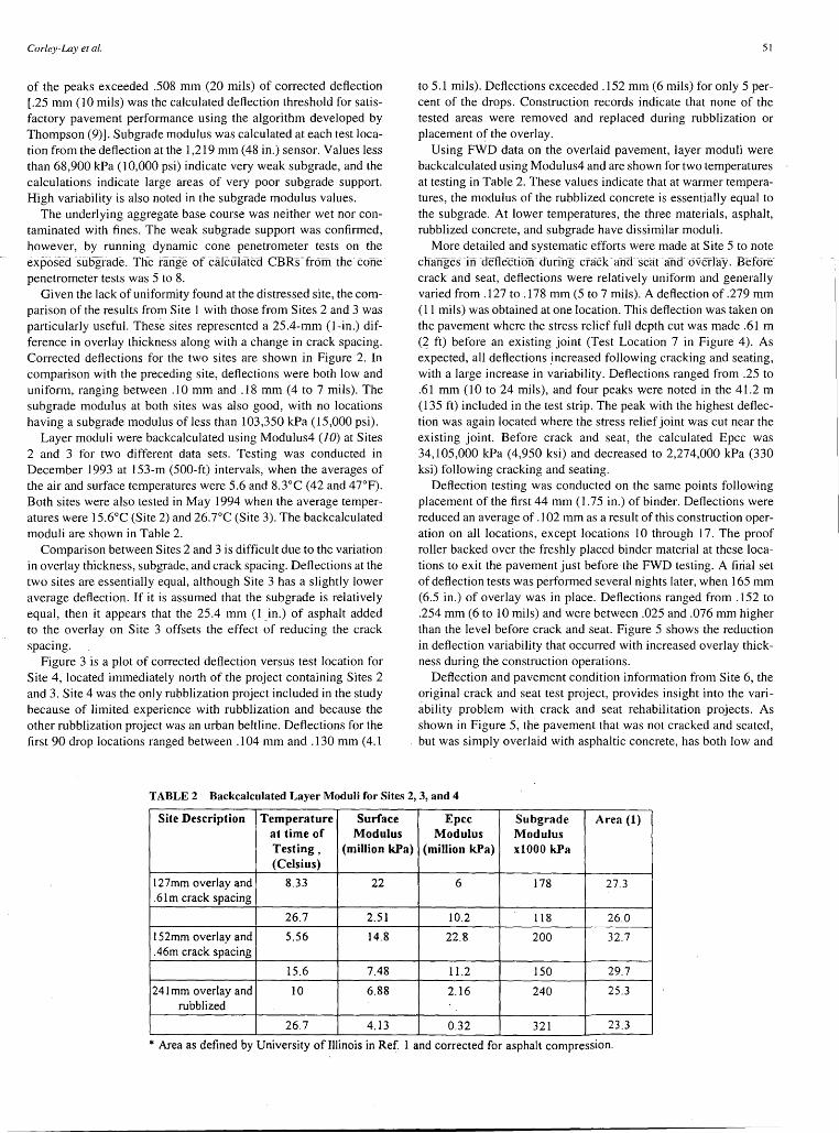
Corley-Lay et al.

of the peaks exceeded .508 mm (20 mils) of corrected deflection [.25 mm (10 mils) was the calculated deflection threshold for satisfactory pavement performance using the algorithm developed by Thompson (9)]. Subgrade modulus was calculated at each test location from the deflection at the 1,219 mm (48 in.) sensor. Values less than 68,900 kPa (10,000 psi) indicate very weak subgrade, and the calculations indicate large areas of very poor subgrade support. High variability is also noted in the subgrade modulus values.

The underlying aggregate base course was neither wet nor contaminated with fines. The weak subgrade support was confirmed, however, by running dynamic cone penetrometer tests on the exp-os-ed -su6grade. The r-ang~e of calculated CBRs-from the- cone penetrometer tests was 5 to 8.

Given the lack of uniformity found at the distressed site, the comparison of the results from Site 1 with those from Sites 2 and 3 was particularly useful. These sites represented a 25.4-mm (I-in.) difference in overlay thickness along with a change in crack spacing. Corrected deflections for the two sites are shown in Figure 2. In comparison with the preceding site, deflections were both low and uniform, ranging between .10 mm and .18 mm (4 to 7 mils). The subgrade modulus at both sites was also good, with no locations having a subgrade modulus of less than 103,350 kPa (15,000 psi).

Layer moduli were backcalculated using Modulus4 (10) at Sites 2 and 3 for two different data sets. Testing was conducted in December 1993 at 153-m (500-ft) intervals, when the averages of the air and surface temperatures were 5.6 and 8.3°C (42 and 47°F). Both sites were also tested in May 1994 when the average temperatures were 15.6°C (Site 2) and 26. 7°C (Site 3). The backcalculated moduli are shown in Table 2.

Comparison between Sites 2 and 3 is difficult due to the variation in overlay thickness, subgrade, and crack spacing. Deflections at the two sites are essentially equal, although Site 3 has a slightly lower average deflection. If it is assumed that the subgrade is relatively equal, then it appears that the 25.4 mm (1 _in.) of asphalt added to the overlay on Site 3 offsets the effect of reducing the crack spacing.

Figure 3 is a plot of corrected deflection versus test location for Site 4, located immediately north of the project containing Sites 2 and 3. Site 4 was the only rubblization project included in the study because of limited experience with rubblization and because the other rubblization project was an urban beltline. Deflections for the first 90 drop locations ranged between .104 mm and .130 mm ( 4.1

51

to 5.1 mils). Deflections exceeded .152 mm (6 mils) for only 5 percent of the drops. Construction records indicate that none of the tested areas were removed and replaced during rubblization or placement of the overlay.

Using FWD data on the overlaid pavement, layer moduli were backcalculated using Modulus4 and are shown for two temperatures at testing in Table 2. These values indicate that at warmer temperatures, the modulus of the rubblized concrete is essentially equal to the subgrade. At lower temperatures, the three materials, asphalt, rubblized concrete, and subgrade have dissimilar moduli.

More detailed and systematic efforts were made at Site 5 to note clfanges-in-defle-ction-durihg crack-anel-seat-ancr overlay. Beforecrack and seat, deflections were relatively uniform and generally varied from .127 to .178 mm (5 to 7 mils). A deflection of .279 mm (11 mils) was obtained at one location. This deflection was taken on the pavement where the stress relief full depth cut was made .61 m (~ ft) before an existing joint (Test Location 7 in Figure 4 ). As expected, all deflections increased following cracking and seating, with a large increase in variability. Deflections ranged from .25 to .61 mm (10 to 24 mils), and four peaks were noted in the 41.2 m ( 135 ft) included in the test strip. The peak with the highest deflection was again located where the stress relief joint was cut near the existing joint. Before crack and seat, the calculated Epcc was 34,105,000 kPa (4,950 ksi) and decreased to 2,274,000 kPa (330 ksi) following cracking and seating.

Deflection testing was conducted on the same points following placement of the first 44 mm (1. 75 in.) of binder. Deflections were reduced an average of .102 mm as a result of this construction operation on all locations, except locations 10 through 17. The proof roller backed over the freshly placed binder material at these locations to exit the pavement just before the FWD testing. A firial set of deflection tests was performed several nights later, when 165 mm (6.5 in.) of overlay was in place. Deflections ranged from .152 to .254 mm (6 to 10 mils) and were between .025 and .076 mm higher than the level before crack and seat. Figure 5 shows the reduction in deflection variability that occurred with increased overlay thickness during the construction operations.

Deflection and pavement condition information from Site 6, the (_)riginal crack and seat test project, provides insight into the variability problem with crack and seat rehabilitation projects. As shown in Figure 5, the pavement that was not cracked and seated, but was simply overlaid with asphaltic concrete, has both low and

TABLE 2 Backcalculated Layer Moduli for Sites 2, 3, and 4

Site Description Temperature Surface Epcc Subgrade Area (1) at time of Modulus Modulus Modulus Testing, (million kPa) (million kPa) xlOOO kPa (Celsius)

127mm overlay and 8.33 22 6 178 27.3 . 61 m crack spacing

26.7 2.51 10.2 118 26.0

152mm overlay and 5.56 14.8 22.8 200 32.7 .46m crack spacing

15.6 7.48 11.2 150 29.7

241 mm overlay and 10 6.88 2.16 240 25.3 rubblized

26_7 4.13 0.32 321 23.3

* Area as defined by University of Illinois in Ref 1 and corrected for asphalt compression.

52

relatively uniform deflections. The deflections were also approximately equal for both the 127-mm and the 190.5-mm (5-in. and 7.5-in.) overlay for the unbroken pavement. Distress data from this portion of the project do not support the optimistic deflection results. Reflective cracking was reported at nine locations in 1993, and the number had increased fourfold by the spring of 1994. Low severity longitudinal cracking and moderate rutting were also observed in this section. The higher level of distress for the uncracked control section is consistent with results reported by Stoffels and Kilareski (1 J).

Low and relatively uniform deflections were also observed for the portion of Site 6 that was cracked and seated with a 1.22-m (48-in.) crack spacing. Four reflective cracks were observed in this section in 1994, along with reflective cracking of the mainline/shoulder edge joint. High severity fatigue cracking was noted in both lanes of both directions at the end of the test section where the asphalt thickness was tapered to meet the adjoining pavement.

Higher and less unifqrm deflections were obtained for crack spacings of .15, .46, and .76 m (6, 18, and 30 in.). The graph of deflections for both eastbound and westbound directions for uniform FWD test spacing of 76.3 m (250 ft) (Figure 6) shows two main peaks in the section having .15-m crack spacing. The magnitudes of these peaks are about .254 mm and .508 mm (10 mils and 20 mils).

. Three peaks, with magnitudes of .279, .508, and .940 mm, were obtained in the variably spaced FWD deflections. Pavement condition was relatively equal for the two directions, with low severity longitudinal and transverse cracking noted most frequently in the outside wheelpath.

Deflection results at 76.3-m (250-ft) intervals for the .46-m (18-in.) crack spacing are both uniform and low in the eastbound direction. Several high deflection peaks are seen for the westbound direction over a total distance of 91.5 m (300 ft). The condition survey for these very high deflection areas indicate high and moderate severity fatigue, moderate severity longitudinal cracking, and multiple full depth patches. This failed area occurred where crack and seat operations were extended beneath an overpass. Clearance was deficient, so the overlay was tapered under the structure, and the failure occurred throughout the tapered area. Damage was present and equally severe in both the eastbound and westbound directions, but was "skipped over" with the test frequency used in the eastbound direction.


A similar but less dramatic peak is noted for the .76-m (30-in.) crack spacing section. Variably spaced deflections recorded the high deflections, peaking at . 787 mm (31 mils), over a 61-m (200-ft) distance. This westbound peak occurred between test locations for the eastbound direction. Again, both directions had similar amounts and severity of distresses consisting of low severity longitudinal and transverse cracking on pavement leading up to a bridge.

Table 3 contains the layer moduli backcalculated for Site 6 using Modulus4. Again two data sets at temperatures of 21.1 arid 36. 7°C (70 and 98°F) are presented. For this table, the backcalculations were initially run using a range of feasible values for the asphaltic concrete modulus. When each test section had been run, similar values were obtained. The average of these similar values was then used as a fixed modulus for the asphalt concrete so the results for the broken concrete could be compared more easily. The results indicate that the uncracked slabs have the highest modulus, with smaller-size pieces having incrementally lower moduli. This trend, however, did not carry to the .15-m ( 6-in.) crack spacing for either overlay thickness, suggesting that the cracking process may have been ineffective at this spacing.

CONCLUSIONS

This study helped the North Carolina Department of Transportation improve its understanding of the deflection behavior of crack and seat pavements. While all the sites investigated for this report had been in service for 4 years or less, all sites other than the site tested during construction had experienced more than a million ESALs.

Among the conclusions are the following:

• Decreasing the crack spacing results in a decrease of cracked layer moduli along with a decrease in subgrade moduli. The rubblization produced a twentyfold decrease in Epcc, while crack and seat reduced the Epcc by a factor between 2 and 10, depending on the crack spacing.

• Crack and seat pavement rehabilitation is likely to perform well when subgrade support is uniform and subgrade moduli are consistently above 103,350 kPa (15,000 psi) after cracking. A method to determine the uniformity of the subgrade and uncracked concrete during the design phase is desirable. The FWD may be a

TABLE 3 Backcalculated Layer Moduli for Test Sections at Site 6

Crack Tempera- Surface Epcc Subgrade Overlay Spacing tu re Modulus Modulus Thickness

(m) (Celsius) (million (million (1000 kPa) (mm) kPa) kPa)

None 21.l 4.82 22.1 198 127

None 36.7 2.24 11.4 172 190.5

1.22 21.1 4.82 11.7 141 127

l.22 36.7 2.24 28.9 145 190.5

0.76 21.1 4.82 7.17 89.6 127

0.76 36.7 2.24 22.1 143 190.5

0.46 21.1 4.82 4.61 97.1 127

0.46 36.7 2.24 8.55 114 190.5

0.15 21.1 4.82 6.96 144 127

0.15 36.7 2.24 8.9 102 190.5

Corley-Lay et al.

method to accomplish this, but relatively close test spacings would be required. Testing at 3.05-m (10-ft) intervals was required to detect major areas of weakness on a project already cracked and seated. Testing showed the decrease in subgrade modulus that occurs when the intact concrete is broken, but testing full projects to find areas of subgrade weakness and to verify their effects after crack and seat was not part of this study.

• Small variations in construction activities, including location of stress relief joints and movement of construction equipment, can adversely affect pavement performance, even after placement of multiple lifts of overlay. Improved clarity of specifications and improved communication between designers and construction personnel is essential.

• Special care must be taken during design and construction of pavement leading under and onto bridges. The most severe distresses and the highest deflections for Site 6 occurred either under bridges or on bridge embankments. Tapering overlay thickness under bridges is unacceptable. Improved performance would be achieved by either leaving the concrete uncracked and carrying a minimal overlay under the structure, or removing the pavement under the structure and constructing a full-depth design to give adequate clearance. It is believed that the poorer conditions -noted on bridge embankments are due to poorer quality compaction that results in voids and loss of support.

• Crack and seat should be designed for not less than a 10-year design period to avoid unsuitably thin overlays. It has not been established in this study that the reflective cracking that does occur on cracked and seated pavements significantly affects pavement performance over the design life.

• Use of layer coefficients for cracked slab rehabilitation design leads to equal overlay thicknesses for rubblization and for crack and seat regardless of the crack spacing. As crack spacing was decreased, however, a thicker overlay was required to reduce the deflections to the same level. The minimum and most uniform deflections occurred at sections with longer crack spacing, but transverse reflective cracking was also observed at these locations.

53

REFERENCES

1. Thompson, M. R. NCHRP Synthesis of Highway Practice 144: Breaking/Cracking and Seating Concrete Pavements. TRB, National Research Council, Washington, D.C., 1989.

2. Carpenter, S. H., and M. I. Darter. Field Performance of Crack and Seat Projects. In Transportation Research Record 1215, TRB, National Research Council, Washington, D.C., 1989, pp. 219-231.

3. Kilareski, W. P., and S. M. Stoffels. Structural Overlay Strategies for Jointed Concrete Pavements, Vol. 11: Cracking and Seating of Concrete Slabs Prior to AC Overlay. FHWA-RD-89-143. FHWA, U.S. Department of Transportation, 1990.

4. Darter, M. I., and K. T. Hall. Structural Overlay Strategies for Jointed Concrete Pavements, Vol. JV: Guidelines for the Selection of Rehabilitation Alternatives. FHWA-RD-89-145.

5. Pavement Consultancy Services/Law Engineering. Guidelines and Methodologies for the Rehabilitation of Rigid Highway Pavements Using Asphalt Concrete Overlays. Prepared for NAPA and SAPAE. Beltsville, Md. June 1991.

6. Wells, G. K., J.B. Hannon, and N. H. Predoehl. California Experience with Cracking and Seating of Concrete Pavements. In Transportation Research Record 1307, TRB, National Research Council, Washington, D.C., 1991, pp. 169-179.

7. Jiang, Y., and R. S. McDaniel. Indiana's Study of Cracking and Seating. Better Roads, Jan. 1994, pp. 19-23.

8. Darter, M. I., R. P. Elliott, and K. T. Hall. Revision of AASHTO Pavement Overlay Design Procedures. Report 20-7/39. NCHRP, TRB, National Research Council, Washington, D.C., Sept. 1991.

9. Thompson, M. R. ILLI-PAVE Based Full-Depth Asphalt Concrete Pavement Design Procedure. Proc. Sixth International Conference on Structural Design of Asphalt Pavements, University of Michigan, Ann Arbor, Mich., 1987.

10. Scullion, T., J. Uzan, and M. Paredes. MODULUS: A MicrocomputerBased Backcalculation System. In Transportation Research Record 1260, TRB, National Research Council, Washington, D.C., 1990.

11. Stoffels, S. M., and W. P. Kilareski. Nationwide Performance Study of In-Service Asphalt Concrete Overlays on Cracked and Seated Portland Cement Concrete Pavements. In Transportation Research Record 12 72, TRB, National Research Council, Washington, D.C., 1990, pp. 15-26.


•


Practical Method for Ensuring the Success of Crack and Seat Operations Using the Falling Weight Deflectometer

SAMEH M. ZAGHLOUL, BRIAN J. COREE, AND REBECCA S. MCDANIEL

Cracking and seating (C&S) of rigid pavements before laying asphalt overlays has been extensively used in recent years to control reflective cracks. By inducing small hairline cracks in the portland cement concrete slabs, the potential for reflective cracks is decreased. The performance of the overlayed section highly depends on the cracking pattern developed in the C&S operation. Deflection testing has been used successfully in C&S operations to evaluate the developed cracking pattern. A mechanistic procedure for calibrating the hammer and the roller in C&S operations using falling weight deflectometer (FWD) measurements is presented. This procedure has two phases: (a) determine the hammer parameters (height and spacing) that develop good cracking patterns, full depth cracks with adequate aggregate interlock between the cracked segments and (b) determine the optimum number of passes of a rubber-tired roller. A three-dimensional, dynamic finite element method (3D-DFEM) was used in the analysis to study the effect of crack width and condition on surface deflections. A dynamic loading cycle was used to simulate the FWD loading cycle. Four crack conditions were considered in the analysis: no crack, minor surface cracks, hairline cracks, and wide cracks. A field validation study was conducted to validate the new approach. Four test sections were included in this study. The results of this study are found to be successful. A userfriendly computer program was developed to implement this method. The program can be loaded on the FWD computer. It reads the FWD raw data file and evaluates the cracking pattern. When the desired cracking pattern is achieved, the program searches for the optimum number of passes of the roller.

Cracking and seating (C&S) of rigid pavements before asphalt overlays has been extensively used in recent years to control reflective cracking in the overlays. This method involves cracking the existing portland cement concrete (PCC) slabs into small segments to reduce the relative movement of the slabs. By inducing small hairline cracks in the PCC slabs, the potential for reflective cracking is decreased.

The Federal Highway Administration (FHW A) Pavement Rehabilitation Manual (1) indicates:

. .

The intent of pavement cracking and seating is to create concrete pieces that are small enough to reduce horizontal slab movements to a point where thermal stresses which contribute to reflective cracking will be greatly reduced, yet still be large enough and still have some aggregate interlock between pieces so the majority of the original structural strength of PCC pavement is retained. Seating of the broken slabs after cracking is intended to reestablish support between the subbase and the slab where voids may have existed.

S. M. Zaghloul, Roads Department, Dubai Municipality, United Arab Emirates. B. J. Coree, R. S. McDaniel, Division of Research Indiana Department of Transportation, 1205 Montgomery Street, West Lafayette, Ind. 47906.

Cracking a PCC pavement is the most important step of the rehabilitation technique. In Indiana, it has been found that C&S jobs that have performed well so far are those that have good cracking patterns. Techniques commonly used to evaluate slab cracking include (2): visual examination of dry and wet slabs, coring, picking up slabs for visual examination, and deflection testing. Visual inspection sometimes is misleading and does not guarantee that cracks are fully developed through the slab thickness. Coring and picking up slabs for visual examination are impractical and take a long time. Deflection testing has been used successfully in C&S operations and is recommended by many highway agencies. In Indiana, the Dynaflect is currently used for this purpose. Empirical criteria are involved in the evaluation process. During the last few years, the Indiana Department of Transportation (INDOT) has experienced some equipment-related problems with the Dynaflect. A decision was made to retire the Dynaflect and use the falling weight deflectometer (FWD) in C&S operations. The procedure used with the Dynaflect is not necessarily valid for the FWD.

This paper presents a mechanistic procedure for calibrating the hammer and the roller in C&S operations using FWD measurements. This procedure has two phases:

• Determine the hammer parameters, height, and spacing that develop good cracking patterns, full depth hairline cracks with adequate aggregate interlock between the cracked segments and

• Determine the optimum number of passes of a rubber-tired roller.

FACTORS THAT AFFECT THE CRACKING PATTERN

The cracking pattern must produce hairline cracks that break the PCC slabs into segments without loosening the aggregate interlock between ·these segments. The- pavemenr strength is-reduced· by cracking, but the cracked slabs still function as a load-carrying layer. Excessive cracking can be detrimental to the pavement structure and turn the slabs into rubble, which is not desired. Figure 1 shows different cracking patterns. Factors that influence the cracking pattern include

• Type and size of hammer; • Impact force of hammer, drop height, and spacing between

drops; • Thickness and strength of the existing PCC slabs; and • Condition of the sub grade.

Zaghloul et al. 55

j_, ___ 1 l_I _____ l........_,,I -t

J Poor Cracking Pattern \ (Cracks are no1 Extended

Through the Slab Thickness)

18" - 24" Spacing

l I -' ..._\ ..._\ ..._\ \ ....... \.........__.l_\_l __ \ ___ I ______ \ ........ \ ......... I II \ \ I \ Good Cracking Pattern

(-Hair line €-racks -E-xten de d Through the Slab Thickness)

I I

!.l 11I111 1111111I11I1111111I111~ ) Poor Cracking Pattern '1

(High Cracking Energy)

1 in = 25 .4 mm

FIGURE 1 Different cracking patterns.

Types of hammer commonly used in C&S operations include the pile-driving hammer, the whip hammer, and the guillotine hammer (3). In a previous study conducted in Indian (4), the guillotine and whip hammers were compared. The results of this study showed that the guillotine hammer is superior to the whip hammer in terms of subsequent performance. Based on the results of this study, INDOT allows only guillotine hammers to be used in C&S operations. The current INDOT specifications require that PCC pavements be cracked into strips that are 45. 72 to 60.69 cm (18 to 24 in.) wide, as shown in Figure 1. Cracking a pavement into smaller pieces ( <45.72 cm) is not recommended because it may result in spalling and loss of structural strength. Only transverse cracks are allowed and should extend to the full depth and width of the PCC slabs.

Because of the variables listed above, at least one 120-ft test section is cracked to determine the impact force, height, and spacing of the hammer that will produce a good cracking pattern. The hammer parameters determined from one section may not be suitable for another section. For example, the pavement condition of one traffic direction could be different from that of the other traffic direction. Therefore, it is recommended that the hammer parameters (height and spacing) are determined independently for each direction.

INDOT CURRENT PROCEDURE

Currently, INDOT uses the Dynaflect and empirical criteria to evaluate cracking patterns and to determine the optimum number of passes· of a rubber-tired roller to ensure adequate seating of the cracked slabs. In this method, three single-slab test sections are tested before cracking with the Dynaflect. After the hammer has cracked the first section, a second round of deflection testing is conducted. In this second round of deflection tests, the Dynaflect sensors are positioned so that a crack is located between Sensors 1 and

2. The cracking pattern is considered good if the differences in the deflections of Sensors I and 2 is greater than 11.

For the seating operation, the pavement deflection is measured after the first, third, and fifth passes of the rubber-tired roller. Readings of Sensor 5 (W5) are plotted versus the number of passes. The number of passes after which the curve of W 5 and the number of passes starts to level off or increase is taken as the optimum number of passes, as shown in Figure 2.

THREE-DIMENSIONAL DYNAMIC FINITE ELEMENT ANALYSIS

A three-dimensional, dynamic finite element method (3D-DFEM), ABAQUS (5), was used to simulate the FWD testing during crack and seat operations and to develop a criterion to evaluate the cracking pattern in the field.

Features of the Finite Element Model

A jointed reinforced concrete pavement (JRCP) cross section similar to the typical cross section of an Indiana highway was modeled in this analysis as two 365.76 cm (2-ft) lanes plus 243.84 cm (8-ft) shoulders on either side. The pavement structure consists of three layers: concrete slab, granular subbase, and subgrade. Asphalt shoulders were used in the analysis to be consistent with the typical cross section of an Indiana highway. A three-dimensional finite element mesh (3D-FEM) with variable size openings was created to model the pavement structure. Variable size openings were used to reduce the computer memory requirements and computational time. A smaller mesh spacing was used to provide detailed response predictions where needed.


22

20

18

c: 16 0

n 14 ~ Q) 0 12

10

8

2 3 4 5 6 7 8 Number of Passes

I --- Section 1 _._. Section 2

1 in= 25.4 mm

FIGURE 2 Effect of the number of passes on surface deflection (Dynaflect).

The pavement structure was modeled as a set of layers. Figure 3 shows one of the 3D-FEM meshes used in the analysis. In this example, the subgrade thickness was represented by three elements, the concrete slab was represented by two elements, and the granular subbase thickness was represented by one element. Longitudinal and transverse joints were modeled using gap elements with an initial opening of 9.53 mm (3/8 in.). Depending on the deformed shape of the slabs after loading, the slabs might come in contact and develop friction. Two types of pavements were considered in the analysis: a plain concrete pavement without dowel bars and a rein-

Shoulder Shoulder

~'"~ ~ .~ s <+--< <+--< ...,_) ro C,) s... v

E-< s... ~

forced concrete pavement with dowel bars. Dowel bars and temperature steel were modeled and located at the mid-depth of the slab. The bond stress of one-half of the dowel bar was set to zero. Details of the finite element features used in this analysis are reported by Zaghloul and White (6).

Three conditions were considered for cracks (as shown in Figure 1 ): minor surface cracks extended only few inches in the PCC slabs; hairline cracks extended through the full depth of the concrete slab, with full friction along the crack sides; and wide cracks with openings not less than 2.54 mm (0.1 in.), with no initial friction but

,-.. ..... The FWD Loading Cycle rn 0... -so v s... ::l rn rn v 0'"' s...

0.. 0

I~ .. ...

D- DFEM Loading Cycle

:

~ v Long. Joints L oaded Plate

1 in = 25.4 mm

FIGURE 3 The 3D-DFEM configuration.

'Zaghloul et al.

with possible contact between the crack sides, depending on the deformed shapes.

Pavement materials included in the analysis were divided into four groups: PCC, asphalt concrete, granular materials, and cohesive soils. Elastic-plastic material models were used to model the portland cement concrete, the cohesive soils, and the granular subbase, and a visco-elastic model was used to model the asphalt mixtures of the shoulder. Details of these material models were reported by Zaghloul (7).

Figure 3 shows an actual FWD loading cycle. This loading cycle was modeled using the straight line segments shown in the same figure. The loading cycle was applied as a distributed load on an approximation of a circle, as shown in Figure 3. A set of 3D, 6-node triangle elements was used to approximate the loaded area.

Finite Element Model Verification

Several verification studies were conducted to verify the 3D-DFEM nonlinear, dynamic analysis capabilities. Some of these verification studies are mentioned below. Details of these studies were reported by Zaghloul and White (6,8,9).

The dynamic response was verified by comparing field-measured pavement deflections from loads moving at different speeds and the 3D-DFEM predictions for similar conditions (pavement structure, load magnitude and configuration, and speed). The predictions were in good agreement with measurements (R2 = 0.998). Figure 4 shows the result of this comparison (6).

In another study, the dynamic analysis capabilities of the 3D-DFEM were verified using a FWD data set. Excellent results were obtained from this study. The predicted peak deflections were found to match the measured ones. Also, the deflection history curves (deflection with time) at different offset distances were found to be in good agreement with the measured ones. The absolute sum of errors between the measured and predicted deflections was 6 percent. Figure 5 shows the measured and predicted deflection basins (9).

.f: c 0 u Q)

'; Cl "O Q)

0 =a ~ a..

0.02

0.018

0.016

0.014

0.012

0.01

0.008

0.006

0.004

0.002

R2

= 0.9964 Estimate = 0.961

01+-~-r-~-r-~.,---..-~..-----.,.........----..------..------.~----..J 0 0.002 0.004 0.006 0.008 0.01 0.012 O.Q1 4 0.016 O.Ql a 0.02

Measured Deflection (in)

l in= 25.4 mm

FIGURE 4 Dynamic analysis verification (moving loads).

'F ~ c 0

u Cl>

15 c Cl> () ca 't: :l en

6

5.5

5

4.5

4

3.5

3

2.5

10 20 30 40

Offset Distance (in)

j --- Measured -- 30-DFEM

l in = 25.4 mm

FIGURE 5 Dynamic analysis verification (FWD).

50

EVALUATION OF THE CRACKING PATTERN USING THE FWD

57

60

The effect of cracks/joints on surface deflections as measured using the FWD is shown in Figures 6 and 7. Two sensor configurations were used in the analysis, as shown in Figures 6 and 7. In both configurations, the deflection of two adjacent slabs were measured to evaluate the load transfer efficiency acro~s the crack/joint. For Configuration 1, the ratio of D2 to D1 is a good indication of the load transfer efficiency, while for Configuration 2, the ratio of D 3 to D2

can be used instead. It was found that Configuration 1 is more practical, and it has been used in the subsequent analysis.

Deflection basins of mid-slab and joint loadings are presented in Figure 6. Because of the PCC slab rigidity, the mid-slab deflection basin is almost a straight line. The shape of the mid-slab deflection basin suggests that:

4.5

4

- 3.5 .! e - 3 c 0

j 2.5 ;::: CD

Q 2

1.5

1 0 10

:£bDf 5 7

20 30 40 50 60

Offset Distance (In)

DJ

70

FIGURE 6 Effect of cracks/joints on surface deflection (Configuration 1).

80

58

-.!! e -c 0

1S Cl ;: Cl 0

4.5

4

3.5

3

2.5

2

01

-10 0 10 20 30 40

Offaet Distance (In)

1 in = 25.4 mm

50 60


where CDR =corrected deflection ratio.

The CDR value of a sound, uncracked pavement is expected to approach 1.0, while the corresponding value for a cracked pavement is expected to be significantly different from 1.0. Figure 8 shows four deflection basins as measured with the FWD. Two of these deflection basins are for crack-free slabs and the other two are for slabs with cracks located somewhere between Sensors 1 and 2 of the FWD. The CDR values for the crack-free slabs are 0.96 and 0.97. The corresponding values for the cracked slabs are 0.78 and 0.83. In the same figure, the theoretical ideal deflection basins; straight lines connecting D 1 and D7, are shown. As can be seen from this figure, the actual deflection basins of the crack-free slabs are very close to the theoretical ideal deflection basins, while the actual deflection basins of the cracked slabs are significantly different from the theoretical ideal ones. This significant difference was reflected on the CDR values.

FIGURE 7 Effect of cracks/joints on surface deflection (Configuration 2).

A sensitivity study was conducted using the 3D-DFEM to evaluate the effect of crack width and condition on the CDR value. In this study, the FWD configuration shown in Figure 6 was used. Four crack conditions were considered in the analysis:

• Cracks with zero opening (no cracks), where • Minor surface cracks at the top 5.08 cm (2 in.) of the PCC

slabs, DR = deflection ratio, • Full-depth hairline cracks with openings less than

D; = deflection of the ith sensor, and 1.25 mm (0.05 in.) and with full friction between the crack sides, X; = distance between the center of the load plate and the ith and

sensor. • Wide cracks with openings greater than 1.25 mm (0.05 in.) and

The above equation can be rearranged as follows: with no friction along the crack sides.

5---~~~~~~~~~~~~~~~~~~~~~~~---,

,..........

4.5

4

~ 3.5 s 3 c 0 -()

~ Qi 1.5 0

o-'"-~~--~~--~~---..-~~-..~~--,.~~---,r-~~r-~---1 0 10 20 30 40 50 60 70 80


\-e- CDR=0.83 -+- CDR=0.97 ........- CDR=0.95 -e- CDR=0.78

1 in= 25.4 mm

FIGURE 8 Effect of crack conditions on surface deflection.

'Zaghloul et al.

Effect of Crack Width on FWD .2 Measurements (Crack and Seat) ~ 0.6~--------..,.-------,------,,0:=="1

c .2 0.5 u ~ 0.4 I-69 (1&2) D

Qi 0 0.3 lJ

Cl> u 0.2

~ 0.1 r:-.r-rl"~*"""""'·'""'::h""'"tc,"'"')"'":;J~""'•.~.,..,.~s*'·~k'"'"'·i~.,,.,·~,,.,.;~'"""~R""' .. ~""'@~.,~""'1·:~:; U No Cracks or Minor Surface Cracks I O O 0.05 0.1 0.15 0.2 0.25 0.3 0.35

Crack Width (in)

o No Temp. Steel "' With Temp. Steel

l in = 25. 4 mm

0.4 0.45 0.5

FIGURE 9 Effect of crack width on FWD measurements.

The effect of the crack condition on CDR as predicted using the 3D-DFEM is shown in Figure 9. It was found that as the crack width increases, the CDR value significantly differs from 1.0, as expected. The effect of temperature steel was found to be significant only for wide cracks, as can be seen from Figure 9.

A field validation study was conducted on the CDR ranges predicted from the 3D-DFEM sensitivity analysis. In this study, a pavement section located on-I-74 in Indiana was tested with the FWD. Two cases were considered in the analysis: crack-free midslab deflections and joint deflections, with the joint located between Sensors 1 and 2. For the former case, the CDR values ranged from 0.96 to 1 .003; for the latter case, the CDR values ranged from 1.2 to 1 .3. These numbers agree with the results of the sensitivity study.

10

9

a ..-...... ~ 7 .E ..._,

6 c 0

-+- 5 u Q)

;;::: 4 Q)

a 3

2

59

IMPLEMENTATION OF THE CDR METHOD

A pilot implementation study was conducted to test the CDR method. Four test sections were included in this study. Two of these sections are located on I-69 and the other two are located on I-74 in Indiana. The four pavement sections were tested with the Dynaflect and the FWD. The current INDOT C&S evaluation procedure was used, as well as the CDR method. The after-cracking CDR were calculated and are presented in Figure 9. It was found that the CDR values were in the range of hairline cracks. These results agree with the results obtained from the current INDOT C&S-evaluation -procedure.

OPTIMUM NUMBER OF ROLLER PASSES

After a PCC pavement is cracked as specified, the concrete is seated or embedded into the subbase with a heavy pneumatic roller. The purposes of the seating operation are to ensure that the cracked slabs will not rock or move under traffic loads and to establish support between the cracked slabs and the subbase. A 30- to 50-ton, rubbertired roller is commonly used for this purpose. In general, three to five coverage of a heavy roller are adequate to seat the cracked slabs. A large number of passes are not recommended because overrolling the cracked pavement may distort the interlock between the individual segments.

The optimum number of roller passes is the minimum number of passes after which no significant reduction in the deflection could be achieved by increasing the number of passes. To determine the optimum number of passes, the deflection is measured at different stages: before cracking; after cracking; and after one, three, and five passes. Figure 10 shows the deflection basins of one of the four test sections included in the implementation study. As can be seen from this figure, the reduction in the deflection when the number of passes increased from three to five is negligible. Therefore, the opti-

~

Before Cracking ---+-After Cracking -1 Pass -a-3 Passes ~

5 Passes

10 20 30 40 50 60 70 80


1 in= 25.4 mm

FIGURE 10 Effect of the number of passes on surface deflection (FWD).

60

mum number of passes for this example is 3. Also, there is a significant difference between the before- and after-cracking deflections. It was found from previous C&S jobs that the deflection of a PCC pavement increases by at least 50 percent when a good cracking pattern is achieved. Therefore, the difference between the before- and after-cracking deflections is used as a second check that slabs are adequately cracked.

RECOMMEND A TIO NS

The optimum values of the hammer and roller parameters in C&S operations can be determined using the FWD. The following steps are recommended in crack and seat operations:

1. Before cracking, three 120-ft test sections are marked and tested using the FWD to determine the pre-cracking deflection.

2. The hammer height and spacing are adjusted to initial values. These initial values are assumed based on similar crack and seat jobs.

3. After the first test section is cracked, using the initial setup of the hammer, a light spray of water or flour should be applied to highlight the cracking pattern.

4. A second round of deflection testing is conducted in which cracks are located between two deflection sensors, as shown in Figure 6. The purpose of these deflection tests is to ensure that fulldepth hairline cracks are developed in the slabs, as well as to ensure that there is still good aggregate interlock among the slab segments. The results of this deflection test are evaluated based on the average CDR.

5. If the deflection tests show that the desired cracking pattern has not been achieved, the hammer height and spacing are changed and another test section is cracked. The new hammer height and spacing are selected based on the results of the previous test section. The above steps are repeated until the desired cracking pattern is achieved. The after-cracking deflection should be at least 50 percent higher than the corresponding before-cracking deflection. If this condition is not satisfied, the cracking operation has to be repeated.

6. After achieving the desired cracking pattern, the seating is started. The rubber-tired roller rolls the pavement five times. Deflection tests are conducted after one, three, and five passes of the roller. A plot of the pavement deflection versus the number of passes is developed to determine the optimum number of passes.

A user-friendly computer program is developed to implement this method. The program reads the FWD data file and calculates the CDR values. If the CDR values are in the range of hairline cracks, the program compares the before- and after-cracking deflection basins. If the after-cracking deflections are at least 50 percent higher than the corresponding before-cracking deflections, the cracking operation is considered successful. The deflection basins after one, three, and five passes are compared, and the program


searches for the optimum number of passes using the approach outlined earlier.

SUMMARY

A procedure is developed to use the FWD measurements to calibrate the hammer and roller during C&S operations. 3D-DFEM was used in the analysis to study the effect of crack width and condition on surface deflections. The 3D-DFEM predictions were verified in previous studies with field measurements. In this analysis, a dynamic loading cycle was used to simulate the FWD loading cycle. Four crack conditions were considered in the analysis: no crack, minor surface cracks, hairline cracks, and wide cracks. Also, a method to select the optimum number of passes of a rubber-tired roller is presented. A field validation study was conducted to validate the new approach. Four test sections were included in this study. The results of this study are found to be successful. A userfriendly computer program was developed to implement this method. The program can be loaded on the FWD computer. The program reads the FWD raw data file and evaluates the cracking pattern. When the desired cracking pattern is achieved, the program searches for the optimum number of passes of the roller.

REFERENCES

1. Pavement Rehabilitation Manual. FHWA, U.S. Department of Transportation, Washington, D.C., Sept. 1985.

2. NCHRP Synthesis of Highway Practice 144: Breaking/Cracking and Seating Concrete Pavements. TRB, National Research Council, Washington, D.C., March 1989.

3. Sharpe, G. W., M. Anderson, and R. C. Deen. Breaking and Seating of Rigid Pavements. In Transportation Research Record 1178, Washington, D.C., 1988, pp. 23-30.

4. Harness, M. Cracking and Seating of Concrete Pavement on 1-74. Interim Performance Report IN84-0IB. Indiana Department of Transportation, Division of Research, Sept. 1986.

5. ABAQUS, Finite Element Computer Program, Version 4.9. Hibbitt, Karlsson, and Sorensen, Inc., 1989.

6. Zaghloul, S., and T. D. White .. Non-Linear Dynamic Analysis of Concrete Pavements. Proc., 5th International Conference on Concrete Pavement Design and Rehabilitation, Purdue University, Ind., Vol. 1, 1993, pp. 277-292.

7. Zaghloul, S. Non-Linear Dynamic Analysis of Flexible and Concrete Pavements. Ph.D. thesis. Purdue University, 1993.

8. Zaghloul, S., and T. D. White. Use of a Three-Dimensional Finite Element Program for Analysis of Flexible Pavement. In Transportation Research Record 1388, TRB, National Research Council, Washington, D.C., 1993, pp. 60-69.

9. Zaghloul, S. M., T. D. White, V. P. Drnevich, and B. Coree. Dynamic Analysis of FWD Loading and Pavement Response Using a ThreeDimensional Dynamic Finite Element Program. Nondestructive Testing of Pavements and Backcalculation of Moduli, Vol. 2, ASTM STP 1198 (H. L. Von Quintas, A. J. Bush, and G. Y. Baladi, eds.), American Society for Testing and Materials, Philadelphia, Pa., 1994.

Publication of this paper sponsored by Committee on Pavement Rehabilitation.


Rehabilitation of a Jointed Portland Cement Concrete Pavement on 1-35 (Southbound) in Kay County, Oklahoma

JEROME E D.ALEIDEN, DA:vib A. OotEN~ AND MA.:Ri< D.-SARGENT

As part of the SHRP Long Term Pavement Performance (L TPP) Studies, numerous projects are being constructed to study various design strategies for new and rehabilitated pavements. These studies are referred to as Specific Pavement Studies (SPS). One SPS rehabilitation study specifically targets the rehabilitation of jointed concrete pavements (SPS-6). Specific designs have been prepared and implemented to incorporate seven of the more common concrete pavement rehabilitation strategies, along with a control section. Sixteen such projects are to be constructed around the country. Included in these treatments are asphalt overlays of the jointed concrete both with and without cracking and seating, as well as various other features in an attempt to enhance the performance of these rehabilitation strategies. One of the 16 planned projects was constructed on I-35 in Kay County, Oklahoma, in the fall of 1992. The existing project featured a 0.2-m (9-in.) jointed reinforced concrete pavement, with a 0.1-m (4-in.) sand cushion, over 0.2 m (8 in.) of soil aggregate subbase on a silty clay subgrade. As part of the SHRP LTPP program, performance data have been collected on.each test section before and after construction. Although the experimental sections in Oklahoma have not been in service long, distinctions in performance are already apparent. Performance of the sections in Oklahoma appear to indicate that a 0.1-m (4-in.) asphalt overlay of jointed concrete pavement (JCP) can be expected to exhibit reflection cracking within 2 years under typical interstate traffic. Reflective cracking can be controlled to some extent using sawing and sealing of the asphalt cement overlay and can be controlled even more effectively using rubblizing. One must consider, however, that the performance referenced herein may be unique to environment, subgrade type, and traffic levels, to name but a few.

INTRODUCTION

As part of the SHRP Long Term Pavement Performance (LTPP) Studies, sections of highway are being selected to apply very specific treatments to study various facets of construction (both new and rehabilitation). These projects are referred to as Specific Pavement Studies (SPS). One category, SPS-6, deals with the rehabilitation of jointed concrete pavement (JCP). In 1992, one SPS-6 project was constructed on I-35 in Kay County, Oklahoma.

SPS-6 General Experiment Design

The specific products anticipated from the SPS-6 experiment are included in Table 1 (1). In general, the experiment is intended to

J. F. Daleiden and M. D. Sargent, Brent Rauhut Engineering, 8240 Mopac, Suite 220, Austin, Tex. 78759. D. A. Ooten, Oklahoma Department of Transportation, 200 N.E. 21st Street, Oklahoma City, Okla. 73105-3204.

evaluate some of the more common concrete rehabilitation techniques currently used by state highway agencies (SHAs). Included in this evaluation are the condition of the pavement before overlay, the loading conditions the section is exposed to (including both environment and traffic), and the various treatment applications. The standard SPS-6 experiment design consists of eight test sections, as shown in Table 2 (1). The test sections include

• Two 305-m ( 1,000-ft) long concrete pavement restoration sections, one with retrofitted edgedrains and one without;

• Two break and seat test sections, one receiving a 0.1-m (4-in.) asphalt overlay and the other a 0.2-m (8-in.) asphalt overlay;

• Three sections with a 0.1-m ( 4-in.) asphalt overlay placed on the existing JCP (one with retrofitted edgedrains, one for which joints were sawed in the asphalt overlay directly above the existing concrete joints and then resealed with hot-poured rubber asphalt, and one conventional overlay).

As part of the experiment design, a control section, to which no treatments were applied was also established to provide for comparisons with the other test sections. Three of the eight joints in the control section did, however, receive some patchwork to eliminate existing safety hazards.

Specific Experiment Design for 1-35

The test sections were part of Federal Aid Project Number IR-35-4(148)214 for rehabilitation of pavement in the southbound lanes ofl-35 in Kay County, Oklahoma. This project began approximately 25.75 km (16 mi) south of the Kansas state line and extended south by some 6.5 km ( 4 mi). Traffic levels on this segment ofl-35 were reported at 10,000 vehicles annual average daily traffic (AADT), consisting of approximately 33 percent trucks. 540,000 ESALs were estimated per year in the study. Plans for this project were prepared by the Oklahoma Department of Transportation (DOT) Rural Design Division. A layout of these test sections is provided in Figure 1. It should be noted that the concrete pavement restoration test sections were intended to include full-depth patching, partial-depth patching, pressure grouting, load transfer restoration, diamond grinding, and joint resealing. Evaluations of this project during the plan preparation phase, however, established that partial-depth patching, load transfer restoration, and pressure grouting were not needed. Fault measurements were typically less than 3 mm (0.1 in.), and pavement deflection readings indicated load transfer efficiency at the joints in excess of 90 percent. Simi-


TABLE 1 Key Products of SPS-6

I Product NQ.1 Description I 1 Comparisons and development of empirical prediction models for perfor-

mance of rehabilitated JPC and JRC pavements with different methods of surface preparation, with and without AC overlays, with sawed and sealed joints, with crack/break and seat preparation and different AC overlay thicknesses, and with and without retrofitted drainage.

2 Evaluation and field verification of AASHTO Guide design procedures for rehabilitation of existing JPC and JRC pavements with and without AC overlay, and other analytical overlay design procedures for JPC and JRC pavements.

3 Determination of appropriate timing to rehabilitate JPC and JRC pavements in relation to existing conditions and type of rehabilitation procedures.

4 Development of procedures to verify and update the pavement manage-ment and life-cycle cost concepts in the AASHTO Guide using the performance prediction models developed for rehabilitated JPC and JRC pavements.

5 Development of a comprehensive data base on the performance of rehabilitated jointed concrete pavements for use by state and provincial engineers and other researchers ..

larly, condition surveys, delamination evaluations at the joints, and coring performed during material sampling and field testing failed to identify areas where partial depth patches would be necessary. Henc~, the concrete pavement restoration for the test sections on I-35 was limited to full-depth patching, diamond grinding, and joint resealing with low modulus silicone.

MONITORING

Extensive observations and testing are conducted on all SPS-6 test sections to establish the impact of these rehabilitation treatments on performance. This includes periodic deflection testing, profile measurements, traffic monitoring, and distress surveys.

TABLE 2 SPS-6 Test Sections

Transition of ~

varying length

SPS-6 JC PAVEMENT Section PREPARATION

1 Routine

Maintenance

2 Minimum Restoration

~ Minimum

Restoration

4 Minimum Restoration

5 Maximum Restoration(CPR)

6 Maximum Restoration(CPR)

7 Crack/Break· and Seat

8 Crack/Break and Seat

OTHER

Additional Sections~ · at agency's option

OVERLAY TREATMENTS THICKNESS

0

0

0.1 m (4 in.)

Saw and Seal 0.1 m(4in.) Joints in AC

0

0.1 m (4 in.)

0.1 m (4 in.)

0.2 m (8 in.)

Pavement Surface Distress

Before construction, those highway segments slated for rehabilitation were filmed in October 1991 by a PASCO ROADRECON unit, and manual (visual) distress surveys were conducted in October 1991 and July 1992. The pavement surface before construction exhibited some map cracking; however, coring and delamination tests did not identify any problem areas of potential delamination. Faulting at the joints was fairly minimal [less than 3 mm (0.1 in.) on average]. Only one corner break existed. A high severity corner break was identified on the first joint (12 m into the section) for Section 400604. Two (on Section 400604) to five (on Section 400601) joints were spalled per section, ranging from a total of 1 m of spalling (on Section 400604) to almost 6 m (on Section 400608). The spalling was predominantly low severity (30 percent); however, some moderate and high severity spalls were noted (6 percent each). Forty-eight percent of the joints exhibited no spalling. After construction, the test sections were again filmed by the PASCO ROADRECON unit in March 1993, and manual distress data were collected in November 1992, October 1993, and March 1994.

Surface Profile

The surface profile was measured by both rod and level surveys and a profilometer. Rod and level measurements were taken immediately before construction, and this project was also profiled using

Daleiden et al.

Test Section ___JQ_ Treatment

Routine Maintenance Minlmum_Bestor:ation Minimum Restoration, 0.1 m (4 in.)Over1ay

63

Rubbelized Concrete

Edge Drain Location

400601 400602 400603 400604 400605 400606 400607 400608

Minimum Restoration, 0.1 m (4 in.) Over1ay, Saw & SeaJ Joints Maximum Restoration(CPR)

Io o o I I' I I I 'I Saw and SeaJ Test Section

Jointed Plain Concrete Maximum Restoration(CPR), 0.1 m (4 in.) Over1ay Crack, Break and seat, 0.1 m (4 in.) Over1ay Crack, Break and seat, 0.2 m (8 in.) Overlay

FIGURE 1 4006XX typical section and site layout.

SHRP's high-speed profilometer in January 1992. The high-speed profilometer produces a longitudinal profile for each wheelpath of the travel lane for each test section at 0.15-m (6-in.) increments. Results of this work expressed as International Roughness Index (IRI) values appear in Table 3. As this pavement profile can, to some extent, be considered a reflection of the joint faulting present, fault measurements were taken at each joint (0.3 m and 0.75 m from the lane edge) using a faultmeter. A summary of the fault measurements at each of the joints is included in Table 4.

In addition to rod and level measurements, all test sections were again profiled using the SHRP high-speed ptofilorheter in March 1993. The resulting values of IRI also appear in Table 3.

Deflection Testing

Deflection measurements were taken in late January and early February 1992 using the SHRP falling weight deflectometer (FWD) to evaluate the structural capacity of each test section. The FWD drops a set of weights from three different heights to simulate different levels of wheel loads, ultimately measuring the resulting deflection basins. Measurements were taken at the corners and mid-span of

TABLE 3 Profile Readings

Preconstruction Date Surveyed: 1/14/92

SECTION LEFT RIGHT AVERAGE 400602 2.16 2.05 2.12 400601 1.99 1.80 1.90 400603 1.63 1.55 1.60 400604 1.79 1.88 1.83 400607 1.93 1.53 1.74 400608 1.79 1.42 1.61 400606 1.64 1.58 1.61 400605 1.55 1.39 1.47

Average 1.81 1.65 1.73

!:::< :::;::::)

~ Asphalt Concrete Overlay

each slab edge. Joint/load transfer tests were conducted in the outside wheelpath and mid-slab throughout each test section. A summary of these results for a 9-kip load simulation is provided in Table 5. Deflection measurements were taken again in April 1993 after the treatment applications were complete.

Materials Sampling and Testing

As specified for all SHRP test sections, a thorough ·materials sampling and testing program was established for these sections on 1-35 in Kay County, Oklahoma. Sampling included extractions of 0.1-m (4-in.) and 0.15-m (6-in.) diameter cores, 0.15-m (6-in.) auger probes, and three 1.8 m X 1.2 m (6 ft X 4 ft) test pits to a depth of 0.3 m (12 in.) just below the top of the untreated subgrade. All sampling was conducted by the Oklahoma DOT with the actual laboratory testing work being performed by a testing contractor. Preconstruction sampling was conducted . in June 1992, and postconstruction sampling and testing was conducted on August 31, 1992.

Some problems were encountered with the two 50-mm (2-in.) thick lifts separating during postconstruction sampling. Every effort

Postconstruction Date Surveyed: 3/16/93

LEFT RIGHT AVERAGE 1.12 1.07 1.09 1.93 1.80 1.86 0.74 0.74 0.74 0.85 0.85 0.85 1.09 1.07 1.07 1.28 1.26 1.28 0.95 0.90 0.92 0.71 0.77 0.74 1.08 1.06 1.07


TABLE 4 Joint Faulting Measurements

SECTION JOINT* 0.3m 0.75m SECTION JOINT* 0.3m 0.75 m :..ocATION PRE POST PRE POST ... OCATION PRE POSl PRE POST

400602 12.4 1 0 1 0 400607 15.6 2 1 32 6 0 2 0 34.6 0 3

50.6 5 0 3 0 53.3 4 6 68.4 1 0 0 0 71.7 1 2 88.5 5 1 5 0 90.5 2 5

106.6 4 1 4 1 127.8 0 0 115.4 8 8 8 6 146.6 3 0 124.6 2 -1 1 1 Average: 2 2

144 5 1 6 1 400608 0.1 2 2 162.2 4 1 1 1 9.3 1 2 180.9 2 0 2 -1 18.7 4 2 200.8 2 0 1 0 37.5 1 2

219 7 3 3 1 56.3 1 1 238 2 0 2 0 75.3 1 0

255.9 1 0 0 1 93.7 2 7 274.6 0 0 0 0 112.7 0 3

294 2 3 3 2 131.5 0 0 150.3 2 1

Average: 3 1 2 1 Average: 1 2 400601 0.5 0 0 0 1 400606 16.3 0 2

19.5 0 0 1 1 35 0 2 38 1 2 1 1 45.5 6 8

56.5 1 1 1 1 54.5 6 7 70.3 8 7 1 1 73.3 6 8 87.3 2 2 2 2 91.5 7 7

106.1 1 2 2 2 109.8 2 2 125.5 7 16 7 9 128.3 2 2 144.5 6 7 4 5 147.5 5 3

Average: 3 4 2 3 Averaae: 4 5 400603 18.8 4 2 400605 4.3 6 1 5 1

37.2 0 0 23 6 1 6 1 56.1 1 2 42 8 2 3 0 74.7 2 3 60 2 0 3 0 93.5 1 0 79 2 0 1 0 113 3 1 98 6 0 3 1 132 5 -1 112.3 1 -1 2 0

150.7 2 2 116.3 2 3 2 2 Average: 2 1 130.8 3 1 2 0

400604 12 3 2 150 5 1 2 1 30.6 2 1 167.5 1 1 2 1

50 1 2 187 2 0 1 0 69.6 4 3 205.3 1 0 1 1 87.6 3 3 215 2 0 5 2

107.1 5 8 224.4 1 1 1 2 127 5 5 237 6 1 3 1

143.5 0 0 254.B 1 1 1 1 273.8 0 0 1 0 292.8 4 0 4 0

Averaae: 3 3 Average: 3 1 3 1

* Measured from 0+00 of each test section.

was made to minimize this splitting of samples, and ultimately complete cores were obtained for all but the 0.2-m (8-in.) thick overlays placed on Section 400608. For the 0.2-m (8-in.) overlay, only one complete core was obtained. The 0.2-m (8-in.) overlay was placed with two 80-mm (3-in.) lifts of Type A mix and one 50-mm (2-in.) lift of Type B mix. It was noted that the bottom 80 mm (3 in.) of this overlay was not well bound together, as aggregate dropped from the cores during sampling.

. CONSTRUCTION

The project was let to Cummins Construction Inc. in November 1991. The preconstruction meeting for this project was held January 28, 1992, at the Division Office in Perry, Oklahoma. Although there were numerous questions regarding the work to be accomplished as part of this SPS-6 project, no significant concerns were expressed regarding the accomplishment of the work specified. At

TABLE 5 Summary of Deflection Results

Mean Values ( microns/kPa) Droo Heillht 2 (141.5 k.Pa)

Test Section 1 2 3

Pre .7176 .6898 .6569

400603

Post .5757 .5162 .5010

Pre .9381 .9147 .8795 -----~ -· - - - - -- - ----- - -

400604

Post .7025 .6307 .6122

Pre .6760 .6477 .6114

400606

Post .9473 .8087 .7891

Pre .7538 .7202 .6843

400607

Post 1.8558 1.4084 1.1434

Pre .7734 .7475 .7105

400608

Post 1.0911 .8793 .7866

this stage of the rehabilitation process, the subcontractor responsible for the "cracking and seating" of the concrete fully intended on using conventional equipment. However, the original subcontractor was replaced by another subcontractor, resulting in a change of equipment. The results of this equipment are discussed below.

For ease of construction, the following sequence of operations was agreed to by all parties:. pavement breaking, overlay, retrofit edgedrains, diamond grind, saw, and seal. Pavement breaking was initiated July 27, 1992, on a small section at the beginning of the transition into Test Section 7, the first of the two break-and-seat test sections. It was quickly noted that this equipment was not a traditional concrete breaker device, but rather a resonant frequency breaker (more commonly used for rubblization). A 0.2-m (8-in.) wide resonating foot traveled along the surface of the pavement at a relatively high frequency of approximately 44 beats/sec, shattering the concrete. Although the equipment produced rubblized concrete rather than conventional break patterns for break and seat, it was determined that the equipment met the requirements of the specifications and was therefore allowed to continue.

A 39-ton pneumatic roller was used to seat the rubblized concrete. Two passes were made over each section. (A pass here is defined as one round-trip over a given area of the section.)

Deflection testing was performed on the rubblized test sections July 29, to evaluate the effect of pavement breaking on the stiffness of the test sections. Some trenching was also performed in several locations to visually examine the fracture patterns of the slabs with depth. Both evaluations indicated that the slab had been broken fulldepth. It was interesting to note that the pieces near the surfaces were typically 50 mm X 50 mm (2 in. X 2 in.), whereas the pieces

Sensors 4 5 6 7

.6069 .5599 .4560 .2833

.4690 .4333 .3584 .2338

.8293 .7776 .6536 .4249 -- -- - -- ---- -- - - -- --- -- -- - - - -- - - --

.5770 .5387 .4556 .3063

.5638 .5!'67 .4225 .2671

.7451 .6972 .5910 .3915

.6365 .5876 .4847 .3046

.8658 .6824 .4597 .2641

.6612 .6099 .5045 .3192

.6679 .5747 .4312 .2661

below the reinforcing steel were closer to 0.2 m X 0.2 m (6 in. X 6 in.).

Before initiating the overlay of the break-and-seat sections, these sections were watered down in an attempt to wash away some of the dust and fines that might inhibit bonding of the asphalt concrete to the broken slab. The first 50-mm (2-in.) lift of Type B (surface) mix was placed on Test Section 7 as well as the first 80 mm (3 in.) of Type A mix on Test Section 8 the day following deflection testing.

The plant was a Caterpillar 2000 drum mixer, located 11 ~25 km (7 mi) north of the project, just off of I-35, in Blackwell, Oklahoma. The paver was a Cedar Rapids Greyhound CR461. The tack coat used during paving was an SS-1. A 50:50 dilution ratio was used.

Three rollers were used to compact the hot mix. The breakdown roller was a 20-kip Hyster steel-wheeled vibratory roller, which made two passes over each section. The intermediate roller was a 24-kip Bomag pneumatic roller, which made five passes over each section, The final roller was a 27-kip Hyster steel-wheeled static roller, which made two passes over each section.

The Advanedge® pipe system was used on this project for edge drainage. This system consisted of a 0.05 m X 0.5 m (2 in. X 18 in.) rectangular plastic perforated channel that was encapsulated by a filter fabric. It was placed as close to the slab as possible [typically 0.1 m to 0.2 m (3 in. to 9 in.)], with the top of the channel positioned 30 mm (1 in.) below the top of the slab. The system was installed using a Vermeer saw to cut a trench 0.5 m deep X 0.1 m wide (20 in. deep X 4 in. wide). The Vermeer saw was equipped with an attachment that laid the pipe immediately behind the saw and pushed the sand subbase material excavated back into the hole. The

66

sand was then compacted in place. Laterals were cut through the shoulder at a 91-m (300-ft.) spacing to drain the system off into the shoulder.

The state utilized its survey crews to come out and locate by offset the position of the existing joints in the shoulder and median before beginning overlay work on the saw-and-seal section (400604). The plan was to use these pins as an aid in positioning the saw for cutting new joints in the asphalt overlay directly above the existing joints. Unfortunately, several of the pins were displaced during some of the shoulder work performed by the contractor. The pins located along the median were still available at each of the joints, however; but there was some concern that the saw cuts would not match the joints exactly, if only this one point was used. Similarly, simply measuring the distance from a known joint would require the assumption that exact distances between joints were known. The prospect of coring to locate the joints more exactly was considered, but it was agreed that this would be a fairly timeconsuming, costly, and potentially detrimental process.

Ultimately, the joints were located taking 0.2-m (6-in.) nails and driving them through the 0.1-m (4-in.) overlay. When properly positioned, the nail would be driven into the joint. When not over the joint, the nail would hit the concrete slab and the nail could not be driven in any further. Five of the eight joints were satisfactorily located in this fashion. The remaining three joints had been patched, and the joint openings left after patching were not wide enough to drive the nails into them. The approximate location of these patches were identified based on visual surveys performed prior to overlay. Only the leave joint of a patch was sawed and sealed. One of the patches did however have pins on both sides remaining, which meant that only two joints were of some concern.

It was also proposed by the local field personnel that one joint be sawed intentionally out of position [by 0.10 m (3 in. or 4 in.)] to monitor performance. It was agreed that this could prove informative. A joint was selected in one of the transition areas for this pur-

4 1: 1:

Outside Lane 2 1: 1:

Width 1: 1:

(m) 1=---1:

0 1:

0 20 DISTANCE

4

Outside Lane 2

Width (m)

0

1: 1: 1: 1: 1: 1: 1: F 1:

I 1: I

1 1 1 1 1

I :i I :i I :i I 1 I l"I


pose. It was speculated that if the joint was sawed within 0.1 m (3 in.) of the original, the joint would perform as desired. There was some concern that the potential for spalling of the overlay might exist if the overlay was sawed too far away from the joint in the concrete surface.

Diamond grinding was performed on Sections 400602 and 400605 by Highway Services, Inc., from Rogers, Minnesota. The equipment used was a Cushion Cut diamond grinder. This unit had a 1-m (37.5 in.) wide cutting head with 168 blades and cut nine grooves per 50-mm (2-in.) span, leaving roughly 3-mm (0.1-in.) peaks and 3 mm (0.1 in.) valleys. The unit averaged roughly 122 m/hr (400 ft/hr), or 2 m/min (7 ft/min).

While diamond grinding was being completed, joint sealing was initiated in Section 2. This work progressed fairly rapidly, with two saws being used to open the joints. Immediately after the sawing was completed, the joints were water-blasted, and sand-blasting was performed just before the Dow low modulus silicone sealant was installed. The two saws were used in series, with one sawing one face of the joint and the following saw trimming the other face of the joint. This provided a clean joint to work with when the sawing was completed.

For the sawing and sealing of the joints in the asphalt overlay of Section 4, only one pass of the saw [40 mm in depth X 80 mm in width (1.5 in. X 0.3 in.)] and no cleaning operations were utilized (i.e., no water- or sand-blasting). These joints were sealed with Krafco Roadsaver 222.

With the completion of the sealing work on August 29, all work within the test sections for this SPS project was complete.

PERFORMANCE EVALUATION

The performance of the SPS-6 test sections have been monitored since the construction was completed in the fall of 1992. Three of

r- r-1: 1: 1: 1: 1: 1: 1: 1:

1: 1: i: 1: 1:_ -'-1: 1: i: 1: 1: i:

40 60 80 (METERS)

=I j: ::i 1: ::i 1:

~ 1: 1:

=I 1: :1 --r--=I 1: ::i 1:

I :I I 1: I

80 100 120 DISTANCE (METERS)

140 160

Cracking(Pre Construction)

Reflection Cracks

Original Joints

Patch (Preconstruction)

FIGURE 2 Distress summary for test section 400603 [0.1 m (4 in.) overlay].

4

Outside Lane 2 Width (m)

0 0

4


0 80

!Ui ??7777720!

I I

• 1 ·I

I I I I I I

20 40 DIST-ANCE (METERS)

I . I : I

I . I . I : I : I . I . !

100 120 DISTANCE (METERS)

Sawed and Sealed Joints (Post Construction) Reflection Cracks Original Joints

Patch (Pre Construction)

Cracking (Pre Construction)

60

140

FIGURE 3 Distress summary for test section 400604 [0.1 m (4 in.) overlay, saw and seal].

4

Outside lane 2 Width (m)

0

4

Outside Lane 2 Width

I

0

I I I I I I

(m) --1 I

0 I I I

80

----------.................... ~

I :1 I I :1 :1 I I :1 :1 ! I :1 - :r

I :1

i I :1 ~ I :1

~

I I :1 ~ I

l11 ~I ~ I I


1: 1: I 1: 1: I 1: 1: I 1: 1: I 1: 1: I 1: i: I 1: 1: t--1: r-1: i: 1! 1: I:


Cracking (Pre Construction) Reflection Cracks

Original Joints

Patch (Pre Construction) ~ 7"

FIGURE 4 Distress summary for test section 400606 [0.1 m (4 in.) overlay with drain].

I I I I I I L_

·1 I ..

80

160

I

80

160


4

Outside Lane 2 II Width (m)

0 I I I I

0 20 40 60 80 DISTANCE (METERS)

4

Outside Lane 2

!I Width (m)

0 80 100 120 140 160

DISTANCE (METERS)

.................... Cracking(Post Construction)

.................... Original Joints

~~ ·Patch (Pre Construction)

FIGURE 5 Distress summary for test section 400607 [0.1 m (4 in.) rubblized.with drain].

the five test sections (400603, 400604, and 400606) have already begun to show reflective cracking. Figures 2 through 6 are graphical representations of the distress manifestations observed in March 1994.

leave edge of underlying patches constructed before rehabilitation. Interestingly enough, the reflective cracking took place at 50 percent (four out of eight) of the locations where sawing and sealing was conducted. Test Section 400606 [0.1-m (4-in.) overlay with drain] exhibited reflective cracking at all but one location where an original joint existed under the new overlay. A reflective crack had also developed at the location of an underlying transverse crack. Test Section 400607 [rubblized with 0.1-m (4-in.) overlay and edgedrain] exhibited a very small amount of postconstruction trans-

Test Section 400603 [0.1 m (4 in.) overlay] exhibited reflective cracking at each of the underlying original joints, as well as partially along one edge of a patch. Test Section 400604 [0.1 m ( 4 in.) overlay, saw and seal] exhibited reflective cracking over the original joints where sawing and sealing was performed, as well as over the

4


0 0 20 40

DISTANCE (METERS)

4

Outside Lane 2 Width

(m) 0


60

140

Cracking(Post Construction-none as of 3/30/94)

. . . . . . . . . . . . . . . . . . . . . Original Joints

so

160

FIGURE 6 Distress summary for test section 400608 [0.2 m (8 in.) rubblized with drain].

Daleiden et al.

verse and longitudinal cracking. A very short crack exists at a location where a preconstruction patch is located. Test Section 400608 [rubblized with 0.2-m (8-in.) overlay and edgedrain] exhibited no distress manifestations throughout the test section.

SUMMARY

After examining all of the pre- and postconstruction surface distress data available for these test sections, the rubblized sections are outperforming the othertestsections to date. Jn addition, the original joints in Section 4 have less reflective cracking than similar joints in Sections 3 and 6. However, all but one preconstruction patch joint in Test Section 4· has reflected through the new overlay. Also, the process of saw and seal of the leave joint of a given patch had virtually no effect. Test Section 400608 (rubblized with 0.2-m (8-in.) overlay and edgedrain) outperformed Test Section 400607 [rubblized with 0.1 m (4 in.) overlay and edgedrain]. However, the distress manifestations that appeared on Test Section 400607 are relatively small in quantity. Additional time will determine the actual significance of the additional 0.1 m ( 4 in.) of material in Test Sectiory 400608 from a cost savings standpoint.

69

CONCLUSIONS

After only 2 years of monitoring the SPS-6 project in Oklahoma, distinctions in performance of these test sections are already apparent. Surface distress data, collected during March of 1994, allowed for a general comparison and performance evaluation.

Sawing and sealing does appear to be somewhat effective at minimizing reflective cracking; howeve_r, the unpredictable nature of patches and their responses to load make such a procedure considerably less effective where extensive patching is involved. When comparing the current condition of each test section with the others, it is apparent that the rubblized-test-sections are outperforming-the other test sections.

REFERENCE

1. Specific Pavement Studies: Experimental Design and Research Plan for Experiment SPS-6, Rehabilitation of Jointed Portland Cement Concrete Pavement, FHW A, U.S. Department of Transportation, working paper, April 1989.



Rationalization of Asphalt Paving Work Using Robot Asphalt Paver: ImageProcessing, Fuzzy-Controlled Paver

T. HAGIWARA, S. KINOSHITA, Y. TAKAGI, AND H. MINAMI

A robot paver equipped with image processing system and fuzzy computer controls was developed, resulting in labor savings, reduction of skilled labor and hard manual work, and rationalization of asphalt paving work. Because the paving conditions in Japan change frequently, considerable labor is necessary for paving operations, such as control of paving thickness and width, asphalt mix feeding, and steering operations. This demands a heavy work load and a high level of skill of operators and screedmen; it also affects the work load of subsequent manual operations, such as shoveling and raking. To solve these problems, a robot asphalt paver was developed. By analyzing construction work factors, this total system paver automates, preprocesses material transport, and postprocesses manual operations (such as shoveling and raking). The features of new automatic functions applied to the robot paver are (a) automatic feeding of asphalt mix to the working equipment, (b) automatic control of the paving thickness, (c) automatic screed extension control, (d) automatic steering control, and (e) semiautomation of asphalt-mix receiving process.

The general trend of skilled and experienced workers aging and leaving the workforce, young workers dropping off from the construction industry, and the rapid aging of the workforce continues in Japan. Although road paving work is called mechanical work, the paver has to be operated by two to three skilled operators, and this working system has remained unchanged until today. Also, about seven to eight workers, including rakers, shovel men, and a supervisor, are usually arranged around the paver. Paving work is still a labor-intensive operation depending on manual workers and skilled operators. Japan's paving industry has various aspects of workrelated problems, and it still strongly depends on manual labor and skilled operators.

To solve these problems, the authors have jointly developed a one-man robot asphalt paver with the aim of labor savings and lowering of the level of skill required by the operator. The robot asphalt paver is a total system that automated the preprocesses (material transport), the self processes (asphalt paving), and the post processes (manual operations such as shoveling and raking).

T. Hagiwara, Utilization Promotion Department, Advanced Construction Technology Center, Otowa NS Building, 7F, 2-10-2, Otowa, Bunkyou-Ku, Tokyo 112, Japan. S. Kinoshita, Taisei Rotec Corporation, 3-13-1, Kyoubashi Chuo-Ku, Tokyo 104, Japan. Y. Takagi, Technical Development Department, The Nippon Road Co., Ltd., 11-20, Tamagawa 2 Chome, OtaKu, Tokyo 146, Japan. H. Minami, Control System Engineering Department, Yokohama Development Center, Niigata Engineering Co., Ltd., 27, Shin-Isogocho, lsogu-Ku, Yokohama-Shi, Kanagawa-Ken 235, Japan.

DEVELOPMENT TARGETS

Analysis of Existing Work Processes

The current construction practice with a conventional paver was analyzed to determine the development targets.

• Analysis of current paving work processes. The functions of the conventional paver, operators, screedmen, and workers were analyzed using industrial engineering (IE) techniques and videotaping the paving conditions.

• Performance survey of the paver and finish. Paving work was conducted only by operators and screedmen, and the effect on the operations of the operators and screedmen and on the finish were surveyed.

• Investigation of the operational functions of the paver.

Operators and screedmen were surveyed regarding the operations under various working conditions, and the level of difficulty of machine operations was investigated.

Current Construction Practice

The following problems were identified quantitatively from the results of the analyses:

• The steering and asphalt mix feeding operations account for a large percentage of the work. These two difficult operations are performed simultaneously by the operators and require a high level of skill.

• Transverse movements of the screedman to control the screed and to adjust the screed extension are frequent, and the workload is heavy.

• To ensure a satisfactory level of finishing accuracy, the work heavily depends on rakemen and screedmen for manual labor in the postprocesses.

• The overall work efficiency decreases during the docking of the paver with the dump truck to receive the asphalt mix.

• Irregular work (manual work) occurs at the beginning and the end of the paving work (tapering to the existing road), resulting in a peak work load for the workers.

Functions

From the problems in the current construction, irregular work is a problem that cannot be avoided during construction, but others are problems related to functions of the conventional paver. Therefore,

Hagiwara et al.

these points were taken up as targets for development, and five elements of automation were selected as the functions to be developed, namely: (a) automatic feeding of asphalt mix, (b) automatic control of paving thickness, (c) automatic extension of the screed, (d) automation of steering operation, and (e) semi-automated receiving of asphalt mix.

DEVELOPED CONTROL SYSTEM

The automatic functions of each equipment developed are given below.

Automatic Ultrasonic Type Feeder for Asphalt Mix

Figure I shows the automatic feeding system for asphalt mix. The automatic ultrasonic type feeder (proportional control system) is fitted with ultrasonic sensors at four locations, as shown in Figure 1. The speeds of the left and right bar feeders and screw and the rotation of the extension screw are controlled by the computer to obtain uniform feed of material over the entire screed width. If the feed quantity of the asphalt mix is inadequate, an alarm rings and the motion stops.

Automatic Control System for Paving 1_'hickness

The automatic control system for paving thickness consists of the automatic system for indicating paving thickness and the automatic

Solenoid proportional control valve

Bar feeder

Drive motor

Ultrasonic distance sensor

Fixed screw


Extension screw

Left screed

Right screed

Drive motor

FIGURE 1 Automatic feeding system for asphalt mix.

71

system for adjusting paving thickness. Figure.2 shows the automatic control system for paving thickness.

Automatic System for Indicating Paving Thickness

This system consists of two ultrasonic sensors fitted on the left and right sides of the leveling arm; inclination sensors; travel distance sensors; and a computer that records, processes images, and displays data. It measures the paving thickness automatically all the time and displays the values on the monitor by the driver's seat. The contrQl mode can ge selectecl from the thickn_ess priority control mode based on the height above the subgrade level, and the level priority control mode based on the height above the structure.

Figure 3 shows the algorithm for measurements of paving thickness. The paving thickness Tat point B, when the robot paver travels a distance M from Condition I to Condition 2 is:

T = H2' + o - M tan 0' - HO

Condition I-Measures and calculates the difference in subgrade levels, o, B, and C. Since

HI + o = H2 + M tan 0

o = H2 - H1 + M tan 0

is calculated.

Controller

Screed gate

Paving thickness measuring device

Side level control device

L

FIGURE 2 Automatic control system for paving thickness.

L Ultrasonic sensors

@~HHHnmnHrnmmmrnmrn@:Jj~jpta;;;··cf::··cz-:-;:·:·:·;-c-~0·~t~~r ~:\@ C B A


Inclination Paving thickness sensor measuring arm


FIGURE 3 Paving thickness measurement.



Hagiwara·et al.

Condition 2-If the paver travels a distance M only between B and t,

H2' + o ~HO+ T + M tan 0'

The paving thickness is calculated as:

T = H2' + o - M tan 0' - HO

Automatic Adjusting System for Paving Thickness

This system consists of the side level control device and paving thickness priority control device. The data of the first and second height sensors, the inclination sensors, the travel distance sensors, and the side level sensors are processed by the computer; the pivot cylinder is activated; and the paving thickness is controlled. Figure 4 shows the control block diagram.

Image Processing System Used in Automatic Screed Extension and Automatic Steering Control Systems

Automatic extension screed and steering control systems were developed considering relevancy with the control system and the following points:

73

• To aim for labor savings by using existing structures, lines, and chalk lines as references, and to eliminate the need for new reference settings;

• To use the same sensor for sensing all objects that can be used as references; and

• To use common sensors for automatic screed extension control and automation of steering, thereby minimizing the number of sensors.

Based on the conditions mentioned above, a sensor that uses laser beams and a CCD camera (hereafter called "road-eye") was developeg. The road-eye d~tec_ts _the ~ct,g_e wh~n there is a level difference in the reference line. For flat reference lines, such as chalk lines, only the CCD camera is used, which detects the reference line by bright and dark binary values of the image.

Figure 5 is an example of using a curb stone as the reference line. A laser slit beam is projected from the front side of the curb stone. The CCD camera captures the image, and the computer processes the image. In this image, the edge of the curb stone can be detected because the laser slit beam is at a different level.

Automatic Extension Control Device for Screed Using Image Processing

Figure 6 shows only the screed part of the robot asphalt paver and its motion with time. Sensors are installed at two locations: the front

r----------------------------------------------------------~

First height sensor Hl

Second Height sensor H2

Inclination sensor

Travel distance sensor

Side level H3

AID converter

110 interface

T=

Paving thickness

T

f (Hl. H2. 8 · · · ·)

Computing section

Average value of existing

paving thickness

Ta= I: T/n

Difference between target and actual paving thickness

t=ta-to

Data storage section

-------- -------------------------------------, AID converter

110 interface

Target Value

LO

Control quantity

E=L-LO control value of cylinder Lp=f (E)

Target correction

LO-LO+f (t)

Target correction

'---------------~-----------------------------

Solenoid valve

-

I /

-L

FIGURE 4 Block diagram of automatic system for adjusting the paving thickness.

74

Laser beam projector

/


I CCD camera

Curb stone CCD camera image I

~ Direction of advance

FIGURE 5 Image processing system.

end (Sensor A) and the rear end (Sensor B) of the screed end plate. Both sensors are controlled so that they are always inside (paving side) of the reference line; this is to prevent collision when the reference line is a structure and to prevent the spilling of material outside the reference line when other materials are used as reference lines. Figure 7 shows the block diagram of the control system.

Automatic Steering Control System Using Image Processing

The sensor used to measure the azimuth angle deviation of the robot asphalt paver is the road-eye. The sensing position is behind the swiveling shaft center of the vehicle body, and the road-eye moves opposite to the steering direction at the start of the steering operation. The steering angle must be changed according to the displacement of the line of travel from the reference line~ Under these conditions, fuzzy control was used because framing of control rules by numerical functions was considered difficult.

Figure 8 represents the fuzzy control input/output unit. Fuzzy deduction is performed using three types of input data in fuzzy control, and the steering angle is determined. The two fundamental rules for fuzzy control are

• Variable value travel control. This rule defines the approach of the screed end plate toward the re.ference line. The robot paver

FIGURE 6 Screed motion.

Detects this edge

travels along the reference line according to this rule. In Figure 9, when the distance between the front Sensor A of the screed end plate and the reference line is taken as X 1, and the distance between the rear Sensor B and the reference line is taken as X2, steering control is performed according to this rule such that the deviation in both XI and X2 is 0.

• Parallel travel control. This rule ensures that the screed end plate is parallel to the reference line. This rule is effective and contributes to attaining a good finish of the paving surface and in suppressing overshoot. In Figure 9, steering control is performed so that XI equals X2.

Computer simulation was performed for determining fuzzy rules and creating membership functions. The effects of the control rules were verified and then applied to the robot asphalt paver.

By applying computer simulation travel, it was possible to reduce the time needed to create rules and membership functions, and to minimize the risks of malfunctions; debugging of actual machine; and disturbances, such as tire slips, that hinder the creation of rules and membership functions.

Figure 10 is an example of the computer simulation screen, showing the locus of travel during automatic steering when the sensor on the right side of the vehicle was brought in line with the curb stone (dotted line), and the vehicle was steered from a straight line course to a right curve.

® .. Dlrection of advance

Hagiwara-et al.

Running speed detector ~

Left road eye ~.____

(front and rear)

I I/O ,___

interface Image processing unit ----- .____

-1

Right road eye (front and rear)

Screed extension quantity detecting sensor

FIGURE 7 Control system b•ock diagram.

Front sensor measured value

Rear sensor measured value

Current steering angle

Fuzzy deduction Steering angle

FIGURE 8 Fuzzy control input/output unit.

Direction of advance

t Reference of advance

FIGURE 9 Measurement of azimuth angle.

75

Running ----- ,___ control

valve Controller ,___ I/O

interface Screed

'----- - extension solenoid control valve

AID converter

Semi-Automated Dump Truck Guidance

A large indicator panel was installed in the robot asphalt paver by the driver's seat. The indicator panel has two modes: the docking mode with the dump truck and the material feeding mode. The modes are switched automatically. During the docking mode, the distance remaining to the stop position is displayed on the indicator panel by the distance sensor. When the stop position is reached, "STOP" is displayed on the panel. The robot paver operator can dis- ·

Front sensor A

Rear sensorB

76

FIGURE 10 Simulation screen.

play the lateral displacement on the indicating panel by pressing a button. If a per on or an object comes between the dump truck and the robot paver at this time, an alarm rings. During the material feeding mode, instruction for dump-up, dump-down, and release can be displayed by pressing a button.

OUTLINE DRAWING OF THE ROBOT PA VER

Figure 11 shows the outline drawing of the robot paver. The robot paver has the following features:

• Total weight of 13,000 kg, • Overall length of 6,700 mm, • Overall width of 2,499 mm, and • Engine power of 66 Kw/2,000 rpm.

ON-SITE WORK

Actual field trials were conducted on National Highway 45 tote t the adaptability of the robot paver for on-site work, evaluate developed function , and verify the degree of rationalization of the work.

There were curvature of 120 m and 200 m and the width of the road varied from 6.5 to 7 .0 m at the test site. The mix u ed wa recycled, gap-graded dense a phalt concrete, which in recent year i u ed in the surface layer for repair work in cold regions with heavy nowfalls.

Working Method

The cut-and-cover method generally u ed in conventional repair work in Japan wa u ed a the working method. Becau e the trial work was to be carried out similar to that of repair work, one-half


of the road was kept open for traffic while work was performed on the other half of the road. The work was carried out in accordance with the common specifications of the Ministry of Construction. Construction control standards for ordinary work were followed also.

Arrangement of Workers

Figure 12 shows the arrangement of workers for the paving work. Becau e the work involved repair , the arrangement of workers around the robot paver wa similar to that used in conventional work, and the possibilities for cutting down various manual operations and reducing heavy manual labor during the operation of the robot paver were investigated.

Items Investigated and Descriptions

Table 1 provides the investigation methods and descriptions of the robot functions.

FIGURE 11 Outline drawing of robot asphalt paver.

Hagiwara et al.

Pre process Post process

FIGURE 12 Arrangement of workers.

Results

80

e-10

5 "' "' Cl>

~ 60 :§ OI) c: -~ 50 c...

I

Negative side

Designed paving thickness

' ~ -~ ~ l ~ -~ ~ ..--- ' ~ ~·

-----~)

Positive side I i• Actually measured valuer

O Indicated value 40 I

5 10 l

15 20 Distance (m)

FIGURE 13 Accuracy of paving thickness.

CONCLUSION

I I 25 30

77

For evaluating the performance of the paving, paving thickness, surface smoothness, cross-section profiles, accuracy of the paved ends, and conditions of the paved surface were evaluated. Figures 13 and 14 show part of the results. The thickness of the paved layer is controlled so that the difference between the values indicated on the monitor and the actual values is within ±3 mm.

The accuracy of the paving ends is controlled to ± 5 mm with respect to the reference line. It was confirmed from the field trial that satisfactory control accuracy could be obtained. During the processing of the end part of the construction joints by the center side, automatic screed extension and feeding of the asphalt mix were sati factory, and fini hed shapes also sati tied the required quality without u ing auxiliary worker . Possibilities of reducing the number of auxiliary workers were also confirmed. A satisfactory paved

The authors have verified labor savings, reduction in skilled labor and hard labor, and effective rationalization of work from the re ults of the field trials of the robot asphalt paver. The authors will improve the robot paver to adapt more effectively to the ite conditions and work toward its perfection so that it becomes a commercially viable product.

ACKNOWLEDGMENTS

urface was obtained during the winter time in spite of the heating effect of the screed and asphalt mix. The surface smoothness and density satisfied the construction control standard , and there was no problem in paving quality.

The robot asphalt paver described in this paper was developed jointly by the Tohoku Engineering Office, Tohoku District Bureau, Mini try of Construction; the Advanced Construction Technology Center; Obayashi Road Co., Ltd.; Kajima Road Co., Ltd.; Seiki Tokyu Kogyo Co., Ltd.; Taisei Rotec Corporation; The Nippon Road Co., Ltd.; Nippon Hodo Co., Ltd.; and Niigata Engineering Co., Ltd.

A survey of the workers after the work wa completed confirmed that the work load of the workers was cut down drastically, despite the fact five auxiliary workers performed the work.

TABLE 1 Investigation Methods and Description.

Category Item Description

Operability Feeding of asphalt mix

Robot functions Investigation method/description

Automatic feed Confirmation of ~ible range of of asphalt mix automatic control work

Adjustment of Automatic . . . CODfulnation of fwible range.of. paving thickness control of automatic control work

operation

A<ijUwlient of construction width

Dump truck guidance

Workability Processing of paved end parts Shoveling work

paving thickness

Automatic cODfumation. of feasible range of control of automatic control work paving thickness Autom8tic · · · · · · confirliiatian.· ·c,f "f·easibie.range. ·of screed extension automatic control work

Semi~automatic Operation" StatUS "cind resP<>nse of" process for dumping operation (investigation receiving by questionnaire) asphalt mix Automatic Required range and scope of work screed extension of raking operation (void Automatic feed recording, questionnaire) of ~halt mix R~ range and scope of work

of Shoveling operation (void recording, questionnaire)


1Posittve side

I I I I I I 5 10 15 20 25 30

Distance (m)

FIGURE 14 Automatic screed extension accuracy.

REFERENCES 3. Umeda, R., et al. Development of Robot Asphalt Paver. Proc., 10th Inter-national Automation and Robotics in Construction, 1993, pp. 261-268.

1. Investigation Report on the Development of Automation Technology for Paving Work. Tohoku Engineering Office, Tohoku District Bureau, Ministry of Construction, 1990, 1991, 1992, 1993.

2. Goto, F., and T. Saitoh. Development of Advanced Asphalt Finisher. Proc., 9th International Automation and Robotics in Construction, 1992, pp. 323-332.

Publication of this paper sponsored by Committee on Applications of Emerging Technology.

transportation research recordonlinepubs.trb.org/onlinepubs/trr/1995/1513/1513.pdfsponsorship of...

Documents