transportation research part c - rutgers university

Contents lists available at ScienceDirect

Transportation Research Part C

journal homepage: www.elsevier.com/locate/trc

Position synchronization for track geometry inspection data viabig-data fusion and incremental learning

Yuan Wanga,b,c, Ping Wanga,b,⁎, Xin Wanga,b, Xiang Liuc

a School of Civil Engineering, Southwest Jiaotong University, Chengdu, ChinabKey Laboratory of High-speed Railway Engineering, Ministry of Education, Chengdu, ChinacDepartment of Civil and Environmental Engineering, Rutgers, The State University of New Jersey, NJ, USA

A R T I C L E I N F O

Keywords:Track geometry inspectionRailwayBig dataInformation fusionPosition synchronizationIncremental learning

A B S T R A C T

Track geometry inspection data is important for managing railway infrastructure integrity andoperational safety. In order to use track geometry inspection data, having accurate and reliableposition information is a prerequisite. Due to various issues identified in this research, the po-sitions of different track geometry inspections need to be aligned and synchronized to the samelocation before being used for track degradation modeling and maintenance planning. This isreferred to as “position synchronization”, a long-standing important research problem in the areaof track data analytics. With the aim of advancing the state of the art in research on this subject,we propose a novel approach to more accurately and expediently synchronize track geometryinspection positions via big-data fusion and incremental learning algorithms. Distinguishing itfrom other relevant studies in the literature, our proposed approach can simultaneously addressdata exceptions, channel offsets and local position offsets between any two inspections. To solvethe Position Synchronization Model (PS-Model), an Incremental Learning Algorithm (IL-Algorithm) is developed to handle the “lack of memory” challenge for the fast computation ofmassive data. A case study is developed based on a dataset with data size of 18 GB, including 58inspections between February 2014 and July 2016 over 323 km (200 miles) of tracks belongingto China High Speed Railways. The results show that our proposed model performs robustlyagainst data exceptions via the use of multi-channel information fusion. Also, the position syn-chronization error using our proposed approach is within 0.15 meters (0.5 feet). Our proposeddata-driven, incremental learning algorithm can quickly solve the complex, data-extensive, po-sition synchronization problem, using an average of 0.1 s for processing one additional kilometerof track. In general, the data analysis methodology and algorithm presented in this paper are alsosuitable to address other relevant position synchronization problems in transportation en-gineering, especially when the dataset contains multiple channels of sensors and abnormal dataoutliers.

1. Introduction

Track geometry defects are considered one of the most important factors in operational stability and safety (Esveld, 2001; Higginsand Liu, 2017; Liu et al., 2013; Quiroga and Schnieder, 2012). Track geometry data from track inspection cars is useful for railwaymaintenance. There are multiple inspection channels corresponding to different types of track geometry, and each channel relates to a

https://doi.org/10.1016/j.trc.2018.06.018Received 27 September 2017; Received in revised form 22 June 2018; Accepted 27 June 2018

⁎ Corresponding author at: School of Civil Engineering, Southwest Jiaotong University, Chengdu, China.E-mail address: [email protected] (P. Wang).

Transportation Research Part C 93 (2018) 544–565

0968-090X/ © 2018 Published by Elsevier Ltd.

T

http://www.sciencedirect.com/science/journal/0968090X

https://www.elsevier.com/locate/trc

https://doi.org/10.1016/j.trc.2018.06.018


mailto:[email protected]


http://crossmark.crossref.org/dialog/?doi=10.1016/j.trc.2018.06.018&domain=pdf

specific type of sensor. Taking the GJ-4 track inspection car of the Chinese Ministry of Railways as an example, some track inspectionparameters are listed in Table 1 (Ren et al., 2010). The illustrative sketches of different types of track geometry are shown in Fig. 1.Each channel corresponds to a specific type of track geometry.

There have been many studies based on track inspection data, including data measurement (Haigermoser et al., 2015; Westonet al., 2007; Bocciolone et al., 2007; Tsunashima, 2008), track condition evaluation (Tsunashima, 2008; Alfelor et al., 2001; Sadeghi,2010; Sadeghi and Askarinejad, 2011) and track degradation prediction (Kawaguchi et al., 2005; Bartram et al., 2008; Liu et al.,2010; Xu et al., 2011, 2012; Xu, 2012; Selig et al., 2008). Nearly all the methods and models require high quality inspection data. Theuse of raw track geometry inspection data from the track geometry car is not always valid due to various data issues, such asmeasurement errors, abnormal data outliers and positional errors. Among these errors, milepost positional error is one common issue,requiring extensive effort to match and align the positions of the same inspected location from multiple inspections (Xu, 2012; Seliget al., 2008; Qu, 2012; Xu et al., 2013). This effort is not trivial because of the need for estimating and predicting location-specifictrack geometry deterioration in railroad track maintenance planning. This paper aims to address position synchronization problemfrom different inspection runs, with a high precision and computational efficiency. The research outcomes can be used for all types ofrailway systems, particularly high-speed railways, whose track asset management demands a high accuracy in positional information.

In practice, an initial milepost can be manually selected. The subsequent mileage information is obtained according to therotation angles (by counting the grating encoder impulse number) and the wheel radius (Allotta et al., 2002), as illustrated in Fig. 2a.However, there are inevitable positional errors caused by radial errors of the wheels, faulty encoder output (Qu, 2012), degradedadhesive conditions (Soleimani and Moavenian, 2017, Liu and Bruni, 2015) or track geometry irregularities (Fig. 2d). Due to thesefactors, the positional error accumulates. To address these issues, the Global Positioning System (GPS) (Specht et al., 2017;Tsunashima, 2008; Allotta et al., 2002), Differential GPS (DGPS) (Allotta et al., 2002; Hanreich et al., 2002) and radio-frequencyidentification (RFID) (Yang, 2009) are introduced as an absolute reference to control the accumulation of positional errors.

Even though many advanced techniques and devices are used, the positional errors cannot be eliminated and can sometimes reach100 meters (328 feet). Furthermore, other environmental conditions could lead to abnormal data points. For example, a film of waterfrom rain on the rail-head can cause laser sensor malfunction (Fig. 2c). This kind of abnormal data outlier may influence theperformance of the position synchronization method. In Section 2, we review the related work in the literature that addresses thisresearch problem, the respective merit and limitations of each method and the intended contributions of our proposed new approachto the body of knowledge.

2. Related prior work

Positional errors can be classified into three categories, which are (1) absolute position errors (APE); (2) relative position errors(RPE); and (3) channel-inside position offset (CPO). Since our study focuses on position synchronization of data from different runswith multiple measurement channels, our review focuses on RPE and CPO. It should be noted that position synchronization is onlyfocus on RPE and CPO. The track inspection dataset used in this paper has undergone a preliminary processing based on the KeyEquipment Identification (KEI) model proposed in Xu et al. (2013).

Table 1Selected track inspection parameters and methods.

Channel Type Sketch Map Measurement Method Sensors

1 Gauge Fig. 1 (1) Laser ranging Laser and displacement transducer2 Longitudinal profile (two sides) Fig. 1 (4) Inertial method Accelerometer and displacement transducer3 Alignment (two sides) Fig. 1 (3)4 Crosslevel Fig. 1 (2) Automatic acceleration compensation Accelerometer5 Warp (twist) – Difference of crosslevel with a distance of 3 meters Calculated from crosslevel

Gauge Zero crosslevelCrosslevel

Alignment

Longitudinal profile

top-line of rail

mid-line of rail

Fig. 1. Schematic diagrams of track gauge, crosslevel, alignment and.

Y. Wang et al. Transportation Research Part C 93 (2018) 544–565

545

2.1. Absolute Position Error (APE)

The positional difference of the inspection data compared to its actual position is called the Absolute Position Error (APE). Theabsolute positional accuracy is important when a worker attempts to locate a track defect that is observed in the inspection. The APEmagnitude is determined by absolute reference along the track. Since there are inevitable errors in the selected reference, the APEcannot be eliminated. In addition to using better inspection technologies, researchers have developed mathematical models to dealwith APE. For example, optimization models were established to minimize the sum of the squares of the difference between two setsof selected track geometry data from a certain section (Sui, 2009). Models are established to correct the local offset of curve sectionsbased on the least square method and correlation coefficient (Li and Xu, 2010; Pedanekar, 2006). More recently, a key equipmentidentification model was proposed to correct the APE of track inspection data by combining the real mileage information of trackequipment, which can reduce the APE to under 5 meters (Xu, 2012; Xu et al., 2013). There are more details regarding APE in Vu et al.(2012).

2.2. Relative position error (RPE)

The mileage difference in inspection data between different runs is known as the Relative Position Error (RPE). The RPE existsbecause of uncertain rail-wheel contact profiles for different inspection cars running along the same track section. The magnitude of RPEis determined by comparing the data from multiple inspections. In the scope of this paper, the process to correct RPE is treated as aproblem of position synchronization. The literature concerning RPE is summarized in Table 2. Addressing RPE is one focus of this paper.

Some common issues with the methods mentioned in Table 2 can be summarized as follows:

• A quantitative assessment model of the RPE is lacking. A general approach to address the position error is to observe the coin-cidence of waveforms from graphs (Xu et al., 2013; Sui, 2009; Li and Xu, 2010). Xu (2012) applies two indirect assessments,including the correlation coefficient and summation of gauge change between the measured waveforms of two inspections, toaddress the performance of mileage corrections. Xu et al. (2015) and Xu et al. (2016) present an indirect measurement by usingstandard deviation of the inspection data of different runs. A smaller standard deviation indicates better performance of themodel.

• The reference for position synchronization is determined both subjectively and empirically. Xu et al. (2015), Sui (2009) and Xuet al. (2016) use the latest set of the previous inspection data as a reference to synchronize the current inspection data. Li and Xu(2010) and Pedanekar (2006) use a reference data library or some static files, which are generated by railway operators and willbe updated when maintenance is carried out.

• All the aforementioned methods are based on a default assumption that the inspection data has no data exception issues, or thedataset is thought to be exception-free after preprocessing. However, that is not always the case. Some models may becomeinvalid or even lead to erroneous positioning results, since the position error due to data exceptions in the reference data willspread to current processed data.

• Only a single measurement channel is used for position synchronization in the above literatures. Abnormal data points may existin one channel, but the probability of data exceptions in all channels at the same position is low. The performance can beenhanced by fusing data from multiple channels in one unified model (Section 5.3).

film

Rail

Inspection car

wheel

Rains

Track

Laser sensors

Weather

move

Slipping

Track geometry irregularity

Fig. 2. Positioning principle of the inspection car and the causes of the positional errors. (a) shows the mileage measuring principle; (b) shows thedegraded adhesive conditions that leads to relative slippage between rail and wheel; (c) shows unforeseen influences such as weather; (d) trackgeometry irregularity.


546

Table2

Prev

ious

stud

iesrelatedto

RPE

.

Referen

ceApp

licationscen

arios

Qua

ntitativeassessmen

tmod

elof

RPE

Maintech

niqu

esReferen

ceforpo

sition

sync

hron

ization

Con

side

ration

ofda

taexceptions

Cha

nnelsin

use

Xu(201

2)Railw

ayIndirect

assessmen

tDyn

amic

timewarping

Thelatest

inspection

run

Prep

rocessing

Trackga

uge

Xuet

al.(20

15)

Railw

ayIndirect

assessmen

tDyn

amic

timewarping

Thelatest

inspection

run

Prep

rocessing

Trackga

uge

Sui(200

9)Railw

ayNot

men

tion

edOptim

ization

Thelatest

inspection

run

Not

men

tion

edProfi

le,a

lignm

entor

gaug

e(one

chan

nel)

Lian

dXu(201

0)Railw

ayNot

men

tion

edLe

astsqua

remetho

dReferen

ceda

talib

rary

Not

men

tion

edProfi

le,a

lignm

entor

gaug

e(one

chan

nel)

Peda

neka

r(200

6)Railw

ayNot

men

tion

edCorrelation

coeffi

cien

tStatic

files

Not

men

tion

ed–

Xuet

al.(20

16)

Subw

ayIndirect

assessmen

tDyn

amic

Prog

rammingan

dCross-

correlation

Thelatest

inspection

run

Prep

rocessing

Profi

le,a

lignm

ent,ga

uge,

twist,an

dcross-leve

l(sep

arately)


547

2.3. Channel-inside Position Offset (CPO)

The Channel-inside Position Offset (CPO) is the position difference of inspection channels between different inspection runs. It isderived from differences in the distribution of sensors between different inspection cars. Generally, the sensors are not mounted at thesame location of the inspection car. As illustrated in Fig. 3, two different types of inspection car, Car A and Car B, measure the sametypes of track geometry, C#1 and C#2. The relative distances between the measurement locations of sensors, d1 and d2, can bedifferent. The CPO is the difference between d1 and d2. The existence of CPO between inspection Car A and Car B is caused becausethe two inspection cars are designed differently.

To our knowledge, there are no published studies concerning CPO. The concept of CPO in the aforementioned Xu (2012), Xu et al.(2015), Sui (2009), Li and Xu (2010), Pedanekar (2006) and Xu et al. (2016) does not exist since they only consider the data from asingle measurement channel. On the contrary, in this paper we attempt to deal with data exception issues by fusing data frommultiple sensors into one unified model. Because it is very rare that all sensors malfunction at the same time (unless there areinspection-car-specific failures), multi-sensor fusion can make our proposed algorithm more robust against sensor data outliers inaligning track inspection data positions.

3. Contributions and organization of this paper

Considering all the limitations of the prior research presented in Sections 2.2 and 2.3, this paper develops a novel approach toaddressing the problem of position synchronization via big data fusion and incremental learning algorithms.

Firstly, the local milepost offset and waveform similarity between every two inspection runs are estimated based on definitionsgiven in Section 5.2. Secondly, to deal with data exceptions, the inspection data of multiple measurement channels are fused by MCF-model in Section 5.3. The channel fusion process improves the precision of position synchronization and enhances the robustnessagainst abnormal data. The side-effect is that the required memory and computation time increase a lot comparing to previousmethods (Xu et al., 2015, 2016; Sui, 2009; Li and Xu, 2010; Pedanekar, 2006), where only the data of one single channel is used.

As a countermeasure, in Section 6, we propose the concept of knowledge library, which represents the minimal information refinedfrom the overall information with a high-dimensional structure. The refining process compresses the overall information into severallow-dimensional vectors and matrices by statistical approaches. Whenever a new dataset is obtained from the track inspection car,the RPE and the CPO of the newly measured data are estimated as referring to historical knowledge, and then position synchroni-zation is carried out to reduce the RPE and CPO. In return, the knowledge library will be updated. The implement of the updatingprocess of knowledge library is called IL-algorithm.

For a better understanding of this paper’s work, its organization is illustrated in Fig. 4. The contents with a red border are the maincontributions, which are also summarized as the following six points.

• The inspection data from multiple measurement channels are fused and synchronized through a multi-channel fusion modelestablished in Section 5.3. A quantitative assessment of RPE is achieved through an optimization model proposed in Section 5.4.

• This paper presents a novel approach to dealing with data exceptions through the establishment of three matching criteria withthe thresholds determined through statistical methods presented in Section 5.5.

• The position synchronization operation is achieved through a two-phase interpolation approach presented in Section 5.6.

• An incremental learning algorithm is developed to execute position error estimating, multi-channel fusing and position syn-chronizing processes in Section 6. The required computational time is minimized via these advanced data processing and analyticalgorithms.

• A case study is developed based on real-life data from part of the China High Speed Railway to demonstrate the practical values ofthis research for industrial practice (Section 7).

• The tradeoff between the computation efficiency and the accuracy of position synchronization is discussed in Section 8.

Inspection Car A

Inspection Car B

Different distribution of sensors

Fig. 3. Sketch map of the CPO and track geometries. C#1 and C#2 represent two different types of track geometry; d1 and d2 are the relative distancesbetween the measurement locations of C#1 and C#2, for inspection Car A and Car B, respectively.


548

4. Abbreviations and nomenclature

See Table 3.

5. Methodology

5.1. Technical framework

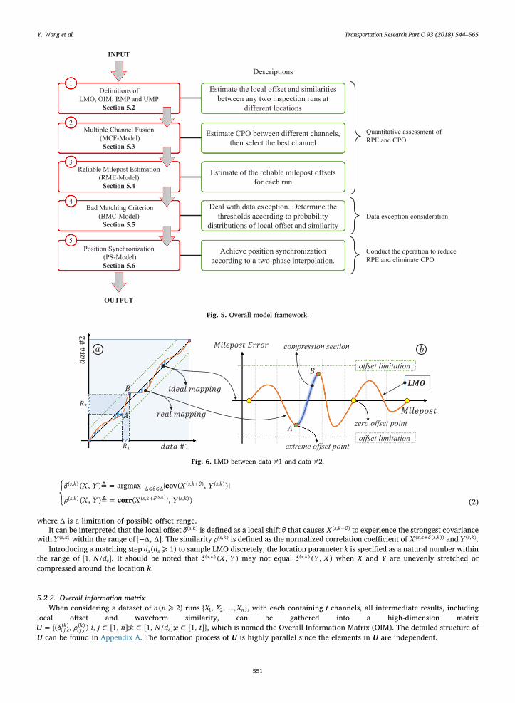
The purpose of this section is to introduce the overall model framework, which contains five parts, one part is model preparationwith some definitions and four sub-models, as illustrated in Fig. 5. The four models, Multiple Channel Fusion Model (MCF-Model),Reliable Milepost Estimate Model (RME-Model), Bad Matching Criterion Model (BMC-Model) and Position Synchronization Model(PS-Model), are established in order of the dependency relationship. The purposes of each process are presented below.

• The first process is aimed at estimating the local offsets and waveform similarities between every two runs of inspection data.(Section 5.2)

• The MCF-Model is established to estimate and fuse the CPO among different inspection channels. (Section 5.3)

• The RME-Model is established to estimate the RPE by fusing the output results of the MCF-Model. (Section 5.4)

• The BMC-Model is established to deal with data exceptions by filtering the CPO and RPE. Three criteria are defined and thethresholds are given according to probability distributions of local offsets and waveform similarities. (Section 5.5)

• The PS-Model is established to conduct position synchronization operation according to a two-phase interpolation. (Section 5.6)

5.2. Fundamentals of the models

This section presents some basic definitions concerning the local offsets between every two runs, including Local Milepost Offset(LMO), Overall Information Matrix (OIM), Reliable Matching Point (RMP) and Unreliable Matching Point (UMP).

5.2.1. Local Milepost OffsetLocal Milepost Offset (LMO) is defined to describe the milepost difference between two data samples, data #1 and data #2 in

Fig. 6. If there is no milepost offset between the two sets of data, this situation is referred to as an ideal mapping, illustrated in Fig. 6a.Real mapping is different from ideal mapping because of RPE. For example, the data sample R1 in data #1 and R2 in data #2 share thesame milepost range, as in curve A-B in Fig. 6a. When R1 is longer than R2, it indicates data #1 is compressed in comparison to data#2 within the A-B range. Therefore, the LMO is defined as the difference between real mapping and ideal mapping, see Fig. 6b.

The following presents a mathematical definition of LMO. For discrete signal = = …X x i N{ | 1, 2, , }i and = = …Y y i N{ | 1, 2, , }i , inconsidering a local waveform matching scale s, the local samples of X and Y at location k are defined as

⎧

⎨⎩

= − + ⩽ < +

= − + ⩽ < +

{ }{ }

X x k i k

Y y k i k

| 1

| 1

s ki

s s

s ki

s s

( , )2 2

( , )2 2 (1)

For ⟨ ⟩i or i N1 , =x y, 0i i the local offset δ s k( , ) and waveform similarity ρ s k( , ) of Y to X are defined as follows

Position Synchronization(PS-Model)Section 5.6

Definitions of LMO, OIM, RMP and UMP

Section 5.2

Multiple Channel Fusion(MCF-Model)Section 5.3

Reliable Milepost Estimation (RME-Model)

Section 5.4

Bad Matching Criterion (BMC-Model)

Section 5.5

OI-AlgorithmSection 6.1

Abbreviations and Nomenclature

Section 5 Section 6

Section 4

Section 3

Contributions and Organization

Section 2

Related Prior Work

Section 1

Introduction AlgorithmsMethodology Discussion

Section 8

IL-AlgorithmSection 6.2

Multi-Channel fusionSection 7.1

Robustness against abnormal dataSection 7.2

Precision and number of iterations Section 7.3

Computational timeSection 7.4

Section 7Case study

Conclusion

Section 9

Tradeoff between execution time and

precision

Fig. 4. Organization of this paper.


549

Table 3Abbreviations and Nomenclature used in this Paper.

Abbreviations Explanation

APE Absolute Position ErrorRPE Relative Position ErrorCPO Channel-inside Position OffsetRMP Reliable Matching PointUMP Unreliable Matching PointRME Reliable Milepost EstimateLMO Local Milepost OffsetOIM Overall Information MatrixMCF-Model Multiple Channel Fusion ModelRME-Model Reliable Milepost Estimate ModelBMC-Model Bad Matching Criterion ModelPS-Model Position Synchronization ModelOI-Algorithm Overall-Iterative AlgorithmIL-Algorithm Incremental-Learning Algorithm

Notation Explanation

s The scale parameter for waveform matchingds The step for waveform matching, 0.25m per point; point by point if ds =1.δ Local mileage offsetρ Local similarity, ranging from [−1, 1].k Refers to a mileage positionc , ∗c A data channel, ∗c indicates the best channel to be selected.

δ X Y( , )s k( , ) The mileage offset of X to Y at location k under scale s.

ρ X Y( , )s k( , ) The similarity of X to Y at location k under scale s.

δij ck,

( ) The mileage offset of the jth run to the ith run at location k based on data from channel c.

ρij ck,

( ) The similarity of the jth run to the ith run at location k based on data from channel c.

XΔ ( )ck( ) , XΔ ( )c The local offset matrix and overall offset matrix at location k based on data from channel c. Where X is a matrix containing data of multiple

runs.

Xϒ ( )ck( ) , Xϒ ( )c The local similarity matrix and overall similarity matrix at location k based on data from channel c. Where X is a matrix containing data of

multiple runs.U = ∈ ∈ ∈δ ρ i j n k N d c t{( , )| , [1, ]; [1, / ]; [1, ]}i j c

ki j c

ks, ,

( ), ,( ) , the Overall Information Matrix. Also written as = …X X c tΔ ϒ{( ( ), ( ))| 1, 2, , }c c .

Ci j c, , The overall channel offset of the jth run to the ith run for channel c.Di c, The estimation of overall channel offset for the ith run.

dik( ), ∗di

k( ) The RME of the ith run at the location k. * indicates the best selected channel.

∗dik( ) The first-order derivative of ∗di

k( ) .

δ0, ρ0, δ1 The thresholds ofδij ck,

( ), ρij ck,

( ) and ∗dik( ) for the BMC.

rUMP=

= ∈ ∈ ∈

U

δi jk ρi j

k i j n k N ds c tcard bo

card

({ ( ,( ), ,

( ) ) 0 | , [1, ]; [1, / ]; [1, ]})

( ), the proportion of the UMPs.

uik n( , ) The average of the LMO of the ith run at location k, considering a total of n runs of inspection data.

nik n( , ) The count of the RMPs of the ith run at location k, considering a total of n runs of inspection data.

K k n( , ) = ∈ ∈u n i j n k N d{( , )| , [1, ]; [1, / ]}ik n

ik n

s( , ) ( , ) , local information matrix.

fr The distribution of variable r, where r can be δ , ρ or d .M A parameter of IL-Algorithm, which represents the maximal number of inspection runs that are to be cached in memory.P p( )r The precision of position synchronization at a given confidence level p.

Operator Explanation

xnorm( ) = = ∑x x‖ ‖ | |i2 2 , vector norm.

x ycov( , ) = ∑ − −x x y y( )( )i i , covariance.x pPercentile( , ) The percentile value of x at a percentage of p.

x ycorr( , ) =− −

x yx yx y

covnorm norm

( , )( )· ( )

, normalized correlation coefficient.

A Bxcorr2( , ) 2D cross-correlation of matrix A and B.card({·}) Number of elements in set {·}.

′x y xinterp( , , ) Resampling the sequence (x y, ) by a new ′x through interpolation.δ ρbo( , )

= ⎧⎨⎩

⩾ ⩽ρ ρ δ δ1, if and | |0, otherwise

0 0 , exception judgment operation.


550

⎧⎨⎩

≜ =

≜ =− ⩽ ⩽

+

+

δ X Y X Y

ρ X Y X Y

cov

corr

( , ) argmax | ( , )|

( , ) ( , )

s kθ

s k θ s k

s k s k δ s k

( , )Δ Δ

( , ) ( , )

( , ) ( , ) ( , )s k( , )(2)

where Δ is a limitation of possible offset range.It can be interpreted that the local offset δ s k( , ) is defined as a local shift θ that causes +X s k θ( , ) to experience the strongest covariance

with Y s k( , ) within the range of −[ Δ, Δ]. The similarity ρ s k( , ) is defined as the normalized correlation coefficient of +X s k δ s k( , ( , )) and Y s k( , ).Introducing a matching step ⩾d d( 1)s s to sample LMO discretely, the location parameter k is specified as a natural number within

the range of N d[1, / ]s . It should be noted that δ X Y( , )s k( , ) may not equal δ Y X( , )s k( , ) when X and Y are unevenly stretched orcompressed around the location k.

5.2.2. Overall information matrixWhen considering a dataset of ⩾n n( 2) runs …X X X{ , , , }n1 2 , with each containing t channels, all intermediate results, including

local offset and waveform similarity, can be gathered into a high-dimension matrix= ∈ ∈ ∈U δ ρ i j n k N d c t{( , )| , [1, ]; [1, / ]; [1, ]}i j c

ki j c

ks, ,

( ), ,( ) , which is named the Overall Information Matrix (OIM). The detailed structure of

U can be found in Appendix A. The formation process of U is highly parallel since the elements in U are independent.

Estimate the local offset and similarities between any two inspection runs at

different locations

INPUT

Definitions of LMO, OIM, RMP and UMP

Section 5.2

Multiple Channel Fusion(MCF-Model)Section 5.3

Reliable Milepost Estimation (RME-Model)

Section 5.4

Bad Matching Criterion (BMC-Model)

Section 5.5

Position Synchronization(PS-Model)Section 5.6

Estimate CPO between different channels, then select the best channel

Estimate of the reliable milepost offsetsfor each run

Deal with data exception. Determine the thresholds according to probability

distributions of local offset and similarity

Achieve position synchronization according to a two-phase interpolation.

1

2

3

4

5

OUTPUT

Descriptions

Quantitative assessment of RPE and CPO

Conduct the operation to reduce RPE and eliminate CPO

Data exception consideration

Fig. 5. Overall model framework.

compression section

extreme offset point

Fig. 6. LMO between data #1 and data #2.


551

5.2.3. Reliable and unreliable matching pointIn practice, for some reasons, such as abnormal data, maintenance carried out by heavy machinery or track condition degradation,

a bad correlation will exist at some milepost points, namely ≪ρ X Y( , ) 1s k( , ) . Therefore, the similarity threshold ρ0 is introduced tojudge whether a matching exception exists at location k. Another situation is also taken as a matching exception when the estimatedlocal offset exceeds a given threshold δ0. The determination of similarity threshold is based on the probability distribution, which is tobe addressed in Section 5.5.4. As a result, the exception judgment operation δ ρbo( , ) is defined as follows:

≜ = ⎧⎨⎩

⩾ ⩽δ ρ

ρ ρ δ δbo( , )

1, if and | |0, otherwise

0 0

(3)

If =δ ρbo( , ) 1i jk

i jk

,( )

,( ) , it indicates that the milepost point at location k is reliable according to the inspection data from the ith and jth

runs; we call this kind of matching point a Reliable Matching Point (RMP). Otherwise it is an Unreliable Matching Point (UMP), andshould be ignored. The ratio between the number of UMPs and the number of all elements in U is denoted as rUMP. The ratio rUMP

represents the proportion of bad matching points. Moreover, the larger the ratio rUMP is, the poorer the repeatability of track geometryis, so that the ratio rUMP is an important index to describe the reliability of position synchronization.

≜ == ∈ ∈ ∈

Ur

δ ρ i j n k N d c tcard bo

card

({ ( , ) 0| , [1, ]; [1, / ]; [1, ]})

( )UMPi j

ki j

ks,

( ),( )

(4)

5.3. Multiple Channel Fusion Model (MCF-Model)

The purpose of this section is to estimate the CPO of each inspection run and establish the model for fusing multiple inspectionchannels. All inspection channels provide information for position synchronization after the corresponding CPO is corrected. Thefusion of multiple channels is the essential part of the models in this paper to deal with data exception.

The estimation of CPO according to the overall information matrix U is presented in Fig. 7. The cube on the left side of Fig. 7represents the overall offset matrix XΔ ( )c1 , please refer to ①. Subscript c1 indicates the channel of gauge. The right cube representsmatrix XΔ ( )ct , see ②. Subscript ct indicates any other channel but that of gauge. The matrixes XΔ ( )c k1, and XΔ ( )ct k, are slices atlocation k of XΔ ( )c1 and XΔ ( )ct , respectively, please refer to ③ and ④. The two vectors δi j c, , 1 and δi j ct, , are extracted from XΔ ( )c1 and

XΔ ( )ct , respectively, please refer to ⑤ and ⑥. In an ideal situation, δi j c, , 1 and δi j ct, , should be coincident, while in actuality there mayexist a constant deviation. The difference between δi j c, , 1 and δi j ct, , is the CPO between the ith and jth run for channel ct, that is denotedas Ci j ct, , .Ci j ct, , , the constant offset of channel ct between the ith and jth run, can be obtained by solving Eq. (5).

= − − = …δ δ C c targmin ‖ ‖ ; 2, 3, ,C i j c i j ct i j c, , 1 , , , ,2

i j ct, , (5)

The best estimation of the channel offset of the ith run, denoted as Di c, , can be obtained by solving Eq. (6).

= − = … = …C D i n c targmin ‖ ‖ ; 1, 2, , ; 2, 3, ,D i j ct i c, , ,2

i c, (6)

Finally, the final local mileage offset ∗δijk( ) between the ith and jth runs at location k can be obtained by subtracting ∗Di c, from ∗δij c

k,

( ) ,

and the final waveform similarity ∗ρijk( ) equals to the one estimated within the channel ∗c , as presented in Eq. (7).

⎧⎨⎩

= −

=

∗

∗

∗ ∗

∗

δ δ D

ρ ρij

kij c

ki c

ijk

ij ck

( ),

( ),

( ),

( )(7)

Fig. 7. Estimation of channel offset.


552

5.4. Reliable Milepost Estimation Model (RME-Model)

The purpose of this section is to establish a model to estimate the reliable milepost offsets for each run of inspection data. All datafrom other inspection runs are taken as a reference to determine the reliable milepost offset for each run. The reliable milepostestimation (RME) of the ith run at location k is denoted as di

k( ). The RME-Model relies on two principles:

• The RME minimizes the sum of squared differences between the ith and other inspection runs;

• The sum of RME of all runs at each location k equals zero.

Therefore, the RME-Model can be described as an optimization model given in Eq. (8).

∑ ∑

∑

⎧

⎨

⎪⎪

⎩⎪⎪

= −

=

= =

∗

=

δ d

d

min ( )

0

i

n

j

n

ijk

ik

i

n

ik

1 1

( ) ( ) 2

1

( )

(8)

Eq. (8) contains an optimization objective and a constrain, which are corresponding to the two principles given above. Eq. (8) is aconstrained least squares problem, which can be solved using the Augmented Lagrangian method, please refer to Appendix B.

5.5. Bad Matching Criterion Model (BMC-Model)

Bad matching points, such as the UMPs, lead to invalid estimations of local offsets and have a great influence on the positionsynchronization of inspection data. Especially in the event of a large erroneous estimation of local offset which is not rectified, thewaveform will distort, the effects of which are all but irreversible. The purpose of this section is to minimize the probability for UMPsto be treated as RMPs through the establishment of the BMC-Model. In this paper, the BMC-Model includes three parts: (1) amplitudecriterion, (2) similarity criterion, and (3) 1st derivative criterion. Multiple criteria can achieve better performance against the faultmatching points.

5.5.1. Amplitude criterionThe amplitude criterion is used for the local offsets, and it works when the magnitude of a local offset is beyond the given

threshold δ0, a limitation not likely to be exceeded. It is especially useful when the inspection data waveform is strongly periodic. Theamplitude criterion is expressed by Eq. (9).

⩽δ δ| |i jk

,( )

0 (9)

5.5.2. Similarity criterionThe similarity criterion is used for the local waveform similarity, and it works when the similarity of two waveforms is sig-

nificantly less than 1. A low similarity indicates unreliable waveform matching. The similarity criterion is expressed by Eq. (10).

⩾ρ ρ| |i jk

,( )

0 (10)

5.5.3. 1st derivative criterionUnlike the above two criteria, the 1st derivative criterion is used for the RME-Model. It works when the change rate of the RME

along the railway is faster than a given threshold δ1, a limitation not likely to be exceeded. The 1st derivative criterion is expressed byEq. (11).

⩽∗d δ| |ik( )

1 (11)

where ∗dik( ) is the first order derivative of ∗di

k( ) along the railway, namely the change rate of the RME. ∗dik( ) is defined by Eq. (12). It

should be noted that, when <δ 11 , the 1st derivative criterion is able to guarantee the monotonicity of the newly generated positioncoordinates in Section 5.6.

=∗ ∗dk

d dd

( )ik

ik( ) ( )

(12)

5.5.4. Determination of δ0, ρ0 and δ1The amplitude threshold δ0 and similarity threshold ρ0 are determined based on the joint probability distribution of δ and ρ. As

the δ0 becomes larger, it is more likely for a UMP to be mistakenly taken as an RMP. Generally, for a lager local milepost offset, thecorresponding similarity will also be larger. In practice, the aim to reduce the probability of false matching can always be achieved byincreasing the values of the thresholds δ0 and ρ0.

The joint probability distribution of the local milepost offset and similarity is illustrated in Fig. 8. The log-normal distribution of ρ


553

is given in N− ∼ −ρ(1 ) ln ( 2.9, 0.8 )2 . In this paper, the thresholds δ0 and ρ0 are given according to the 99% confidence level, or stricter

95% confidence. As for the threshold δ1, the distribution of ∗dik( ) can also be obtained from the overall information matrix U.

Similarly, the value of δ1 can be obtained according to the 99% confidence level, or stricter 95% confidence.It should be noted that the confidence level can be taken as a percentage threshold, which is given empirically according to

subjective experience. Higher confidence level leads to more misjudgments of Reliable Matching Points (RMPs) and fewer mis-judgments of Unreliable Matching Points (UMPs), and vice versa. The percentage should not be too large or too small. In this paper,two percentages are suggested, 95% and 99%.

5.6. Position Synchronization Model (PS-Model)

The purpose of this section is to establish a model to conduct position synchronization according to the estimated RPE and CPO.Assuming ∗di

k( ) is the best estimated mileage offset of the ith run at location k, the position synchronization can be achieved bymoving the data point from location k to a new location of + ∗k di

k( ) . The channel offset Di c, for different runs needs to be included toensure channel synchronization. The process can be described as a two-phase interpolation approach that can be written as Eq. (13).

= + + = … = …∗ ∗X d d d D d X d i n c tinterp interp( ( , , ), , ); 1, 2, , ; 1, 2, ,i c m m ik

i c v i c v,( )

, , (13)

where ∗Xi c, is the synchronized data, and = …d N(1, 2, , )vT . = − + = …d i d i N ds{( 1)· 1| 1, 2, , / }m s , is the matching position sequence

with a step of ds.The first interpolation (the inside interpolation in Eq. (13) is aimed at generating a new position coordinate according to the

mapping of d d( , )ori new . Since the new position coordinate does not share the same sampling rate with that of the original, the secondinterpolation (the outside interpolation in Eq. (13)) is conducted to achieve data resampling by dv. Piecewise linear interpolation isadopted in the first interpolation, while both piecewise linear interpolation and cubic spline interpolation can be used in the secondinterpolation.

The PS-Model process is illustrated in Fig. 9. The solid line in Fig. 9(a) represents the estimated RME of one run of inspection data.The estimated ∗di

k( ) are taken as a discrete sampling of RME. The piecewise linear interpolation for the first interpolation of Eq. (13) isequivalent to a linear approximation of the RME. The second interpolation of Eq. (13) can reduce the RME, as shown in Fig. 9(b). Theresidual RME is the interpolation remainder of the first interpolation of Eq. (13).

For ∈x x x[ , ]0 1 , the linear interpolation remainder is expressed as:

=′

− −R xf ξ

x x x x( )( )2

( )( )0 1 (14)

It can be seen from Eq. (14) that, theoretically, the residual RME will converge towards 0 as −x x| |1 0 approaches 0. In this paper, thevalue of −x x| |1 0 equals the matching step ds. However, the smaller −x x| |1 0 is, the more calculations there will be. The optimization ofcomputation efficiency and precision will be discussed further in Section 8.

6. Computational algorithms

The purpose of this section is to develop algorithms to achieve the estimating, fusing and synchronizing processes. A directsolution is proposed in this paper through an Overall-Iteration Algorithm (OI-Algorithm). As an improvement, the Incremental-Learning Algorithm (IL-Algorithm) is developed to handle the “lack of memory” and massive computation challenges.

Fig. 8. The joint probability distribution of local milepost offset and waveform similarity. (b) Is an enlarged view of the range in the highlightedsquare of (a). The scattered points in the highlighted circles indicate the UMPs.


554

6.1. OI-Algorithm

Considering that deviations may exist in the RME values due to distortions of the original waveform in the inspection data, insteadof simply decreasing the matching step ds, further iterations of the PS-Model on the newly processed results can more efficientlyenhance the position synchronization performance. According to Eq. (14), the farther the position is to the interpolation points, thelarger the residual RME becomes. A new iteration for position synchronization can be better when it avoids the previous RMPs. It isachieved in this paper by changing the beginning position of the matching sequence dm according to the iteration number, as in Eq.(15).

= ⎧⎨⎩− + − + = … = … ⎫

⎬⎭∗d i d j s

Ni N

dsj N( 1)· ( 1)· 1 1, 2, , ; 1, 2, ,m s

oo

(15)

where ∗dm represents the matching sequence with multiple iterations; No is the overall number of iterations; j is the iteration number.As a result, the OI-Algorithm, which takes the simultaneous input of data from all inspection runs, contains several iterations and

in each iteration the four models are solved in order. A new iteration is carried out on the results of the previous iteration (or theoriginal data for the first iteration). The flow chart of the OI-Algorithm is presented in Appendix C.

The implement of OI-Algorithm is exactly corresponding to the data processing flow provided in Fig. 5, the overall model fra-mework. From the calculation steps illustrated in Fig. 17, it can be found that the input dataset will undergo the five sub-proceduresgiven in Sections 5.2-5.6, one after the other until the final result is obtained.

Though the OI-Algorithm is a complete implementation of the four models presented in Section 5, there are two main challengesfor practical application of the algorithm.

• Challenge 1: lack of memory. Take a 300 km track section for example, the required buffer memory reaches 12 GB to cache thedata of 50 inspection runs. More memory is needed to carry out the OI-Algorithm. The size of the overall information matrix U is50× 50×10,000× t for a matching step of 30m, where t is the number of inspection channels in use. U is larger when pro-cessing data from more inspection runs.

• Challenge 2: massive computations. Each time a new inspection run is conducted, the OI-Algorithm needs to be re-executedwith massive repeated calculations. A direct countermeasure can be helpful to reduce repeated computation, such as storing thematrix U. Nevertheless, with an increasing number of inspection runs, it is uneconomical to store such a quantity of intermediarydata.

An incremental algorithm is of great importance to achieve the models instead of the OI-Algorithm. The aim is not simply totransform the OI-Algorithm into an incremental style, but to minimize the required memory, and optimize computations throughincremental probability estimation and the establishment of a “Knowledge Library”.

6.2. IL-Algorithm to improve the OI-Algorithm

6.2.1. Knowledge libraryIn fact, it is not necessary to store all elements in the overall information matrix U. The concept of a “knowledge library”

represents the minimal information refined from the high-dimensional matrix U. The refining process compresses U into several low-dimensional matrices or vectors through statistical approaches. Each time a new set of data is obtained from the track inspection car,

Fig. 9. Illustration of the PS-Model process.


555

the RPE and CPO of the newly measured data is estimated by reference to the historical knowledge. In return, the knowledge will beupdated.

The knowledge library contains two parts: local knowledge and global knowledge. Local knowledge is the refined informationfrom the overall information matrix U for different inspection runs at different locations; this process is shown in Fig. 10.

XΔ ( )ck( ) represents the slice of XΔ ( )c at location k. It should be noted that the UMPs should not be included, so the values δij

k( ) areexcluded when =δ ρbo( , ) 0ij

kij

k( ) ( ) . The average and the number of elements in the ith row of XΔ ( )ck( ) , denoted as ui

k( ) and nik( ) re-

spectively, are taken as local knowledge, as shown in Eq. (16).

∑

∑

⎧

⎨

⎪⎪

⎩⎪⎪

=

=

=

∗ ∗ ∗

=

∗ ∗

u δ ρ δ

n δ ρ

bo

bo

( , )·

( , )

ik

nj

n

ijk

ijk

ijk

ik

j

n

ijk

ijk

( ) 1

1

( ) ( ) ( )

( )

1

( ) ( )

ik( )

(16)

The value of ∗ ∗δ ρbo( , )ijk

ijk( ) ( ) equals 1 for a RMP, and 0 for a UMP, so ni

k( ) is calculated by summing up ∗ ∗δ ρbo( , )ijk

ijk( ) ( ) directly for

= …j n1, 2, , .Global knowledge retains the overall features of the matrix U, including the statistical distributions of δ, ρ and d , that are denoted

as f p[ ]δ , f p[ ]ρ and f p[ ]d , respectively. The range =L r δ ρ d( , , )r can be divided into ′N2 parts. The number of parameters in each part pare counted according to Eq. (17).

⎜ ⎟= ⎛⎝⎧⎨⎩ ′

⩽ <+′

⎫⎬⎭⎞⎠

= − ′ − ′ … ′−N rp

NL r

pN

L p N N Ncard1

; , 1 , , 1r p r r, ,1 ,2(17)

where the boundaries of δ, ρ, and d are given as:

⎧

⎨⎪

⎩⎪

= −= −= −

LLL

[ Δ, Δ][ 1, 1][ Δ , Δ ]

δ

ρ

d

,(1,2)

,(1,2)

,(1,2) 1 1 (18)

The total number of elements in U is = ⩽ <N r L r Lcard({ | })r r r,1 ,2 . Global knowledge f p[ ]r can be calculated according to Eq. (19).

=f pNN

[ ] ;rr p

r

,

(19)

6.2.2. Incremental implementation of the RME ∗dik( )

According to Appendix B, the result ∗dik( ) consists of two parts, ′di

k( ) and ∗d k( ) , the incremental implementation of ∗dik( ) can

therefore be derived from two parts, as expressed in Eq. (20).

∑= ′ − = −+

∗ ∗ +

=

++d d d u

nu1

1ik

ik k

ik n

i

n

ik n( ) ( ) ( ) ( , 1)

1

1( , 1)

(20)

the

Fig. 10. The refining processing for local knowledge.


556

It should be noted that the ∗dik( ) in Eq. (20) is the total estimation of reliable mileage offset based on the historical inspection data.

When the data of the (n+ 1)th inspection run is included, the adjustment value is given in Eq. (21).

∑= − = − −+⎛

⎝⎜ − ⎞

⎠⎟

+ ∗ ∗ ∗ +

=

++d d d u u

nu u( ) 1

1ik n

ik

ik n

ik n

ik n

i

n

ik n

ik n( , 1) ( ) ( , ) ( , 1) ( , )

1

1( , 1) ( , )

(21)

where +unk n

1( , ) is defined as zero because there is no previous information for the (n+1)th run.

6.2.3. Local knowledge updatingThe updating process of local knowledge contains four parts, as presented in Fig. 11.

Process A. Obtain the local milepost offset = …+∗

+∗δ ρ i N{( , )| 1, 2, , }i n

ki n

k, 1( )

, 1( ) by performing the waveform matching for data of the

(n+1)th run to each of the previous n runs, respectively, using the model presented in Section 5.2.1.Process B. Obtain the local milepost offset = …+

∗+∗δ ρ i N{( , )| 1, 2, , }n i

kn i

k1,

( )1,

( ) by performing the waveform matching for each of theprevious n to (n+1)th runs, respectively, using the model presented in Section 5.2.1.

It should be noted that the aforementioned data from the previous n runs are the latest version after mileage synchronization.

Process C. The matrix K k n( , ) is updated into +K k n( , 1) with = …+∗

+∗δ ρ i N{( , )| 1, 2, , }i n

ki n

k, 1( )

, 1( ) . The formula is as follows:

⎧

⎨⎪

⎩⎪

= +

= +

++ + +

++ +

+u n u δ ρ δ

n n bo δ ρ

bo( · ( , )· )

( , )

ik n

n ik n

ik n

i nk

i nk

i nk

ik n

ik n

i nk

i nk

( , 1) 1 ( , ) ( , ), 1( )

, 1( )

, 1( )

( , 1) ( , ), 1( )

, 1( )

ik n( , 1)

(22)

Eq. (22) is an incremental form of Eq. (16). The mean value +uik n( , 1) is updated based on the previous value ui

k n( , ) and the newlyinput +δi n

k, 1( ) .

Process D. The (n+1)th row of +K k n( , 1) is generated with = …+∗

+∗δ ρ i N{( , )| 1, 2, , }n i

kn i

k1,

( )1,

( ) . The formula is as follows:

∑

∑

⎧

⎨

⎪⎪

⎩⎪⎪

=

=

++

=+∗

+∗

++

=+∗

+∗

++u δ ρ δ

n δ ρ

bo

bo

( , )·

( , )

nk n

nj

n

n jk

n jk

ijk

nk n

j

n

n jk

n jk

1( , 1) 1

11,

( )1,

( ) ( )

1( , 1)

11,

( )1,

( )

nk n

1( , 1)

(23)

Eq. (23) is similar to Eq. (16), because there is no previous knowledge for the (n+1)th inspection dataset.

6.2.4. Global knowledge updatingThe global knowledge updating process can be achieved as Eq. (24).

Fig. 11. Local knowledge updating process.


557

= + =++

+f pN

f p N N r δ ρ d[ ] 1 ·( [ ]· ); , , r

n

rn r

nr

nr p

n( 1)( 1)

( ) ( ),

( 1)

(24)

where

= ⎛⎝ ′

⩽ <+′

= + ⎞⎠

+ { }N rp

NL r

pN

L iorj ncard |1

; 1r pn

ij r ij r,( 1)

,1 ,2(25)

= + ⩽ < = ++N N r L r L iorj ncard({ | ; 1})rn

rn

ij r ij r( 1) ( )

,1 ,2 (26)

6.2.5. IL-AlgorithmThe flow chart of the IL-Algorithm is presented in Fig. 18 in Appendix D. The initialization of the knowledge library can be

achieved by applying the OI-Algorithm on M inspection runs. After the data of the (n+1)th inspection run is processed ( ⩾n M), thedata of the ( + −n M1 )th inspection run is saved to the disk and released from memory, so there are only +M 1 inspection runs ofdata in memory. Each time data from a new inspection run is imported, the four models are to be solved using the newly processedhistorical data, rather than the original measured data. It should be noted that in this paper the data arrival order is arrangedaccording to the inspection date. The early inspection data is processed before the late one.

There are two main improvements in the IL-Algorithm compared to the OI-Algorithm:

• The IL-Algorithm only needs to cache data from M inspection runs, rather than all historical inspection data as in the OI-Algorithm. The parameter M is determined according to the required precision and hardware environment, such as memorycapacity.

• Instead of caching the entire matrix U, only the knowledge library needs to be cached in memory. The knowledge library isupdated incrementally with few redundant calculations during the execution process of the algorithm.

7. China high speed railway case study

The purpose of this section is to demonstrate the performance and contribution of the proposed track inspection data positionsynchronization methodology. It should be noted that there are a lot of results to be presented corresponding to the models given inSection 5. However, this section only presents the most important and interesting points due to limited space. This section focuses onfour aspects, that are (1) multi-channel information fusion, (2) robustness against data exception, (3) precision and number ofiterations, and (4) computational time. The precision of position synchronization is defined as the percentile value of the estimatedLMO (δi j

k,( )) at a given confidence level p, as given in Section 5.5.4.

A case study was carried out based on a dataset with 58 inspection runs (17.7 GB) between February/2014 and July/2016 on theChina High Speed Railway. Each inspection run contained 13 measurement channels, including milepost, gauge, crosslevel, long-itudinal profile (left and right side), alignment (left and right side), superelevation, curvature, carbody acceleration (vertical andlateral direction), speed and ALD (please refer to Xu et al., 2013 for a description of ALD). The length of the railway line was 323 km.The sampling distance of the inspection car was 0.25m. Some default parameters of the IL-Algorithm are: matching scale s=50m;matching step ds= 20m; matching range Δ=40m and percentage threshold for BMC-Model is 99%. The dataset has undergonepreliminary processing using the Key Equipment Identification (KEI) model proposed in Xu et al. (2013).

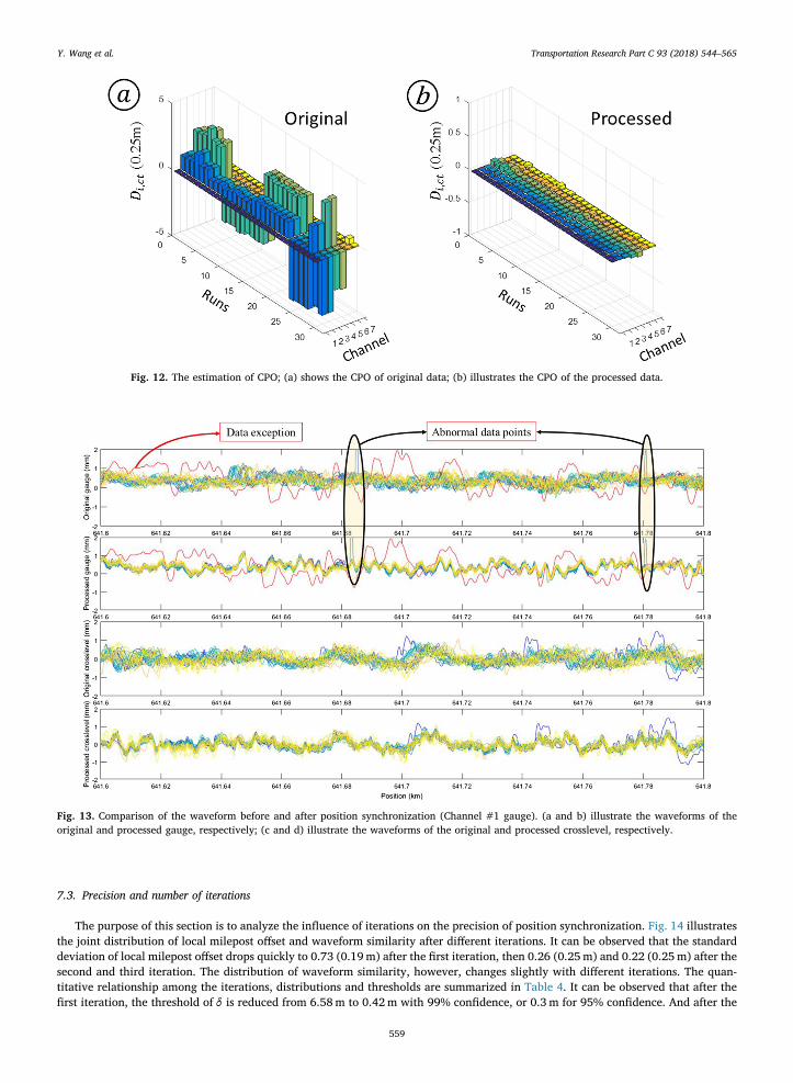
7.1. Multi-channel information fusion

Fig. 12 illustrates the estimated CPO of the original and processed inspection data. It can be found that the CPO of the originalchannel offset is within the range of [−1.25, 1.25] meters by reference to the gauge channel, as illustrated in Fig. 12(a). There aredifferences between different runs and channels. As for the processed data, the CPO drops to less than 0.025m, which can never-theless be disregarded, as found in Fig. 12(b).

7.2. Robustness against abnormal data

This section presents a comparison between the waveform before and after position synchronization. The inspection data fromtwo channels, Channel #1 for track gauge and Channel #2 for crosslevel, within the range of K641.6-K641.8 are taken as an example,please refer to Fig. 13.

It can be seen that Channel #1 (gauge) has some abnormal data points, which randomly occurred in different inspection runs, ashighlighted in Fig. 14(a), (b). And there are data exceptions in the measured gauge of the inspection run colored red, see Fig. 13(a),(b). By contrast, Channel #2 (crosslevel) does not have any abnormal data points within the same range of positions. As a result, theUMPs in Channel #1 are substituted by the RMPs in Channel #2 through multi-channel fusion. That explains the robustness of themethods in this paper against abnormal data for the synchronized gauge.


558

7.3. Precision and number of iterations

The purpose of this section is to analyze the influence of iterations on the precision of position synchronization. Fig. 14 illustratesthe joint distribution of local milepost offset and waveform similarity after different iterations. It can be observed that the standarddeviation of local milepost offset drops quickly to 0.73 (0.19m) after the first iteration, then 0.26 (0.25m) and 0.22 (0.25 m) after thesecond and third iteration. The distribution of waveform similarity, however, changes slightly with different iterations. The quan-titative relationship among the iterations, distributions and thresholds are summarized in Table 4. It can be observed that after thefirst iteration, the threshold of δ is reduced from 6.58m to 0.42m with 99% confidence, or 0.3 m for 95% confidence. And after the

Fig. 12. The estimation of CPO; (a) shows the CPO of original data; (b) illustrates the CPO of the processed data.

Fig. 13. Comparison of the waveform before and after position synchronization (Channel #1 gauge). (a and b) illustrate the waveforms of theoriginal and processed gauge, respectively; (c and d) illustrate the waveforms of the original and processed crosslevel, respectively.


559

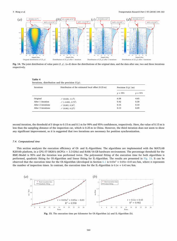
second iteration, the threshold of δ drops to 0.15m and 0.1m for 99% and 95% confidences, respectively. Here, the value of 0.15m isless than the sampling distance of the inspection car, which is 0.25m in China. However, the third iteration does not seem to showany significant improvement, so it is suggested that two iterations are necessary for position synchronization.

7.4. Computational time

This section analyzes the execution efficiency of OI- and IL-Algorithms. The algorithms are implemented with the MATLABR2016b platform, in a CPU/I7-5820 k (6CPUs×3.3 GHz) and RAM/16 GB hardware environment. The percentage threshold for theBMC-Model is 95% and the iteration was performed twice. The polynomial fitting of the execution time for both algorithms isperformed, quadratic fitting for OI-Algorithm and linear fitting for IL-Algorithm. The results are presented in Fig. 15. It can beobserved that the execution time for the OI-Algorithm (developed in Section 6.1 is + −n n0.03 0.05 0.032 sec/km, where n representsthe number of inspection times. In contrast, the execution time for the IL-Algorithm is +n0.1 0.43 sec/km.

Fig. 14. The joint distribution of value pairs δ ρ( , ). (a–d) show the distributions of the original data, and the data after one, two and three iterationsrespectively.

Table 4Iterations, distribution and the precision P p( )r .

Iterations Distribution of the estimated local offset (0.25m) Precision P p( )r (m)

=p 99% =p 95%

Original N (0.020, 11.3 )2 6.58 4.65After 1 iteration N −( 0.001, 0.73 )2 0.42 0.30After 2 iterations N (0.003, 0.26 )2 0.15 0.10After 3 iterations N (0.002, 0.22 )2 0.13 0.09

Fig. 15. The execution time per kilometer for OI-Algorithm (a) and IL-Algorithm (b).


560

8. Discussion

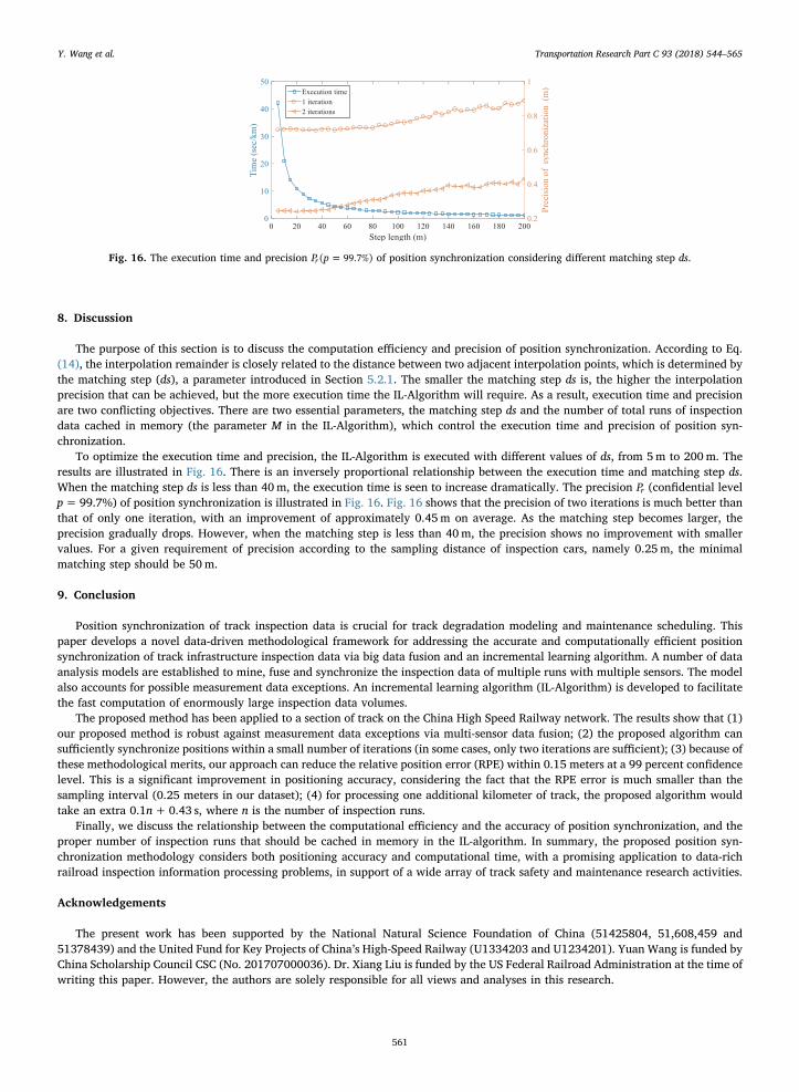
The purpose of this section is to discuss the computation efficiency and precision of position synchronization. According to Eq.(14), the interpolation remainder is closely related to the distance between two adjacent interpolation points, which is determined bythe matching step (ds), a parameter introduced in Section 5.2.1. The smaller the matching step ds is, the higher the interpolationprecision that can be achieved, but the more execution time the IL-Algorithm will require. As a result, execution time and precisionare two conflicting objectives. There are two essential parameters, the matching step ds and the number of total runs of inspectiondata cached in memory (the parameter M in the IL-Algorithm), which control the execution time and precision of position syn-chronization.

To optimize the execution time and precision, the IL-Algorithm is executed with different values of ds, from 5m to 200m. Theresults are illustrated in Fig. 16. There is an inversely proportional relationship between the execution time and matching step ds.When the matching step ds is less than 40m, the execution time is seen to increase dramatically. The precision Pr (confidential levelp=99.7%) of position synchronization is illustrated in Fig. 16. Fig. 16 shows that the precision of two iterations is much better thanthat of only one iteration, with an improvement of approximately 0.45m on average. As the matching step becomes larger, theprecision gradually drops. However, when the matching step is less than 40m, the precision shows no improvement with smallervalues. For a given requirement of precision according to the sampling distance of inspection cars, namely 0.25m, the minimalmatching step should be 50m.

9. Conclusion

Position synchronization of track inspection data is crucial for track degradation modeling and maintenance scheduling. Thispaper develops a novel data-driven methodological framework for addressing the accurate and computationally efficient positionsynchronization of track infrastructure inspection data via big data fusion and an incremental learning algorithm. A number of dataanalysis models are established to mine, fuse and synchronize the inspection data of multiple runs with multiple sensors. The modelalso accounts for possible measurement data exceptions. An incremental learning algorithm (IL-Algorithm) is developed to facilitatethe fast computation of enormously large inspection data volumes.

The proposed method has been applied to a section of track on the China High Speed Railway network. The results show that (1)our proposed method is robust against measurement data exceptions via multi-sensor data fusion; (2) the proposed algorithm cansufficiently synchronize positions within a small number of iterations (in some cases, only two iterations are sufficient); (3) because ofthese methodological merits, our approach can reduce the relative position error (RPE) within 0.15 meters at a 99 percent confidencelevel. This is a significant improvement in positioning accuracy, considering the fact that the RPE error is much smaller than thesampling interval (0.25 meters in our dataset); (4) for processing one additional kilometer of track, the proposed algorithm wouldtake an extra 0.1n+0.43 s, where n is the number of inspection runs.

Finally, we discuss the relationship between the computational efficiency and the accuracy of position synchronization, and theproper number of inspection runs that should be cached in memory in the IL-algorithm. In summary, the proposed position syn-chronization methodology considers both positioning accuracy and computational time, with a promising application to data-richrailroad inspection information processing problems, in support of a wide array of track safety and maintenance research activities.

Acknowledgements

The present work has been supported by the National Natural Science Foundation of China (51425804, 51,608,459 and51378439) and the United Fund for Key Projects of China’s High-Speed Railway (U1334203 and U1234201). Yuan Wang is funded byChina Scholarship Council CSC (No. 201707000036). Dr. Xiang Liu is funded by the US Federal Railroad Administration at the time ofwriting this paper. However, the authors are solely responsible for all views and analyses in this research.

Fig. 16. The execution time and precision =P p( 99.7%)r of position synchronization considering different matching step ds.


561

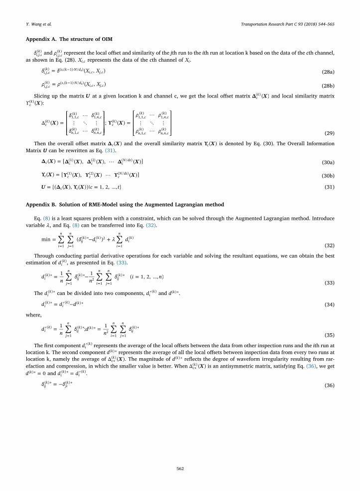
Appendix A. The structure of OIM

δi j ck

, ,( ) and ρi j c

k, ,( ) represent the local offset and similarity of the jth run to the ith run at location k based on the data of the cth channel,

as shown in Eq. (28). Xi c, represents the data of the cth channel of Xi.

= −δ δ X X( , )i j ck s k N d

i c j c, ,( ) ( ,( 1)· / )

, ,s (28a)

= −ρ ρ X X( , )i j ck s k N d

i c j c, ,( ) ( ,( 1)· / )

, ,s (28b)

Slicing up the matrix U at a given location k and channel c, we get the local offset matrix XΔ ( )ck( ) and local similarity matrix

Xϒ ( )ck( ) :

=⎡

⎣

⎢⎢⎢

⋯⋮ ⋱ ⋮⋯

⎤

⎦

⎥⎥⎥

=⎡

⎣

⎢⎢⎢

⋯⋮ ⋱ ⋮⋯

⎤

⎦

⎥⎥⎥

X Xδ δ

δ δ

ρ ρ

ρ ρϒΔ ( ) ; ( )c

kc

kn ck

n ck

n n ck

ck

ck

n ck

n ck

n n ck

( )1,1,( )

1, ,( )

,1,( )

, ,( )

( )1,1,( )

1, ,( )

,1,( )

, ,( )

(29)

Then the overall offset matrix XΔ ( )c and the overall similarity matrix Xϒ ( )c is denoted by Eq. (30). The Overall InformationMatrix U can be rewritten as Eq. (31).

= ⋯X X X XΔ Δ Δ Δ( ) [ ( ), ( ), ( )]c c c cN ds(1) (2) ( / ) (30a)

= ⋯X X X Xϒ ϒ ϒ ϒ( ) [ ( ), ( ) ( )]c c c cN ds(1) (2) ( / ) (30b)

= = …U X X c tΔ ϒ{( ( ), ( ))| 1, 2, , }c c (31)

Appendix B. Solution of RME-Model using the Augmented Lagrangian method

Eq. (8) is a least squares problem with a constraint, which can be solved through the Augmented Lagrangian method. Introducevariable λ, and Eq. (8) can be transferred into Eq. (32).

∑ ∑ ∑= − += =

∗

=

δ d λ dmin ( )i

n

j

n

ijk

ik

i

n

ik

1 1

( ) ( ) 2

1

( )

(32)

Through conducting partial derivative operations for each variable and solving the resultant equations, we can obtain the bestestimation of di

k( ), as presented in Eq. (33).

∑ ∑ ∑= − = …∗

=

∗

= =

∗dn

δn

δ i n1 1 ( 1, 2, , )ik

j

n

ijk

i

n

j

n

ijk( )

1

( )2

1 1

( )

(33)

The ∗dik( ) can be divided into two components, ′di

k( ) and ∗d k( ) .

= ′ −∗ ∗d d dik

ik k( ) ( ) ( ) (34)

where,

∑ ∑ ∑′ = ==

∗ ∗

= =

∗dn

δ dn

δ1 ; 1i

k

j

n

ijk k

i

n

j

n

ijk( )

1

( ) ( )2

1 1

( )

(35)

The first component ′dik( ) represents the average of the local offsets between the data from other inspection runs and the ith run at

location k. The second component ∗d k( ) represents the average of all the local offsets between inspection data from every two runs atlocation k, namely the average of ∗ XΔ ( )c

k( ) . The magnitude of ∗d k( ) reflects the degree of waveform irregularity resulting from rar-efaction and compression, in which the smaller value is better. When ∗ XΔ ( )c

k( ) is an antisymmetric matrix, satisfying Eq. (36), we get=∗d 0k( ) and = ′∗d di

ki

k( ) ( ).

= −∗ ∗δ δijk

jik( ) ( )

(36)


562

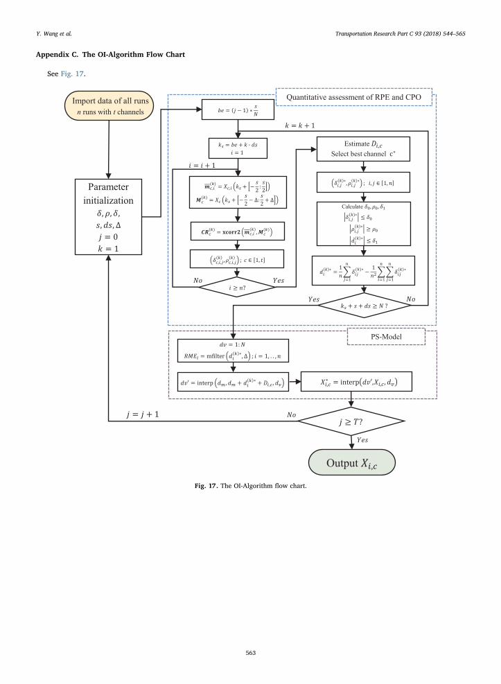
Appendix C. The OI-Algorithm Flow Chart

See Fig. 17.

Fig. 17. The OI-Algorithm flow chart.


563

Appendix D. The IL-Algorithm Flow Chart

See Fig. 18.

Fig. 18. The IL-Algorithm Flow Chart.


564

References

Alfelor, R.M., Carr, G.A., Fateh, M., 2001. Track degradation assessment using gauge restraint measurements. Transp. Res. Rec. 1, 68–77.Allotta, B., Colla, V., Malvezzi, M., 2002. Train position and speed estimation using wheel velocity measurements. Proc. Inst. Mech. Eng. Part F J. Rail Rapid Transit

216 (3), 207–225.Bartram, D., Burrow, M., Yao, X., 2008. A Computational Intelligence Approach to Railway Track Intervention Planning. Evolutionary Computation in Practice.

Springer, Berlin Heidelberg.Bocciolone, M., Caprioli, A., Cigada, A., Collina, A., 2007. A measurement system for quick rail inspection and effective track maintenance strategy. Mech. Syst. Sig.

Process. 21 (3), 1242–1254.Esveld, C., 2001. Modern Railway Track. Delft University of Technology Publishing Service, The Netherlands, pp. 349–406.Haigermoser, A., Luber, B., Rauh, J., Gräfe, G., 2015. Road and track irregularities: measurement, assessment and simulation. Veh. Syst. Dyn. 53 (7), 878–957.Hanreich, D.W., Mittermayr, P., Presle, G., 2002. Track geometry measurement database and calculation of equivalent conicities of the OBB network. In: Proceedings

of the AREMA 2002 Annual Conference, Washington, DC.Higgins, C., Liu, X., 2017. Modeling of track geometry degradation and decisions on safety and maintenance: a literature review and possible future research

directions. Proc. Inst. Mech. Eng. Part F J. Rail Rapid Transit 095440971772187.Kawaguchi, A., Miwa, M., Terada, K., 2005. Actual data analysis of alignment irregularity growth and its prediction model. Quart. Report of Rtri 46 (4), 262–268.Li, H., Xu, Y., 2010. A method to correct the mileage error in railway track geometry data and its usage. In: 2010 International Conference on Traffic and

Transportation Studies. pp. 1130–1135.Liu, R., Xu, P., Wang, F., 2010. Research on a short-range prediction model for track irregularity over small track lengths. J. Transp. Eng. 136 (12), 1085–1091.Liu, B., Bruni, S., 2015. Analysis of wheel-roller contact and comparison with the wheel-rail case. Urban Rail Transit 1 (4), 215–226.Liu, X., Saat, M.R., Qin, X., Barkan, C.P., 2013. Analysis of U.S. freight-train derailment severity using zero-truncated negative binomial regression and quantile

regression. Accid. Anal. Prev. 59 (59C), 87–93.Pedanekar, N.R., 2006. Methods for aligning measured data taken from specific rail track sections of a railroad with the correct geographic location of the sections, US,

US7130753[P].Qu, J., 2012. Study on Track Irregularity Prediction and Decision-aiding Technology based on TQI of Raised Speed Lines. Ph.D. thesis. Beijing Jiaotong University,

Beijing, China.Yang, A., 2009. Automatic correction milepost system of geometry inspection car based on RFID. Railway Comput. Appl. 18 (10), 39–41 (In Chinese).Quiroga, L.M., Schnieder, E., 2012. Monte Carlo simulation of railway track geometry deterioration and restoration. Proc. Inst. Mech. Eng. Part O J. Risk Reliab. 226

(3), 274–282.Ren, S., Gu, S., Xu, G., Gao, Z., Feng, Q., 2010. Development of GJ-4G track inspection car. Proc. Spie 7544 75440Q–75440Q-6.Sadeghi, J., 2010. Development of railway track geometry indexes based on statistical distribution of geometry data. J. Transp. Eng. 136 (8), 693–700.Sadeghi, J., Askarinejad, H., 2011. Development of track condition assessment model based on visual inspection. Struct. Infrastruct. Eng. 7 (12), 895–905.Selig, E.T., Cardillo, G.M., Stephens, E., Smith, A., 2008. Analyzing and forecasting railway data using linear data analysis. Comput. Railways XI.Soleimani, H., Moavenian, M., 2017. Tribological aspects of wheel-rail contact: a review of wear mechanisms and effective factors on rolling contact fatigue. Urban

Rail Transit 3 (4), 227–237.Specht, C., Koc, W., Chrostowski, P., et al., 2017. The analysis of tram tracks geometric layout based on mobile satellite measurements. Urban Rail Transit 3 (4),

214–226.Sui, G., 2009. Mileage calibration algorithm of track geometry data. J. Transport Inf. Saf.Tsunashima, H., 2008. Condition monitoring of railway tracks using in-service vehicles: development of probe system for track condition monitoring. J. Mech. Syst.

Transport. Log. 3 (1), 154–165.Vu, A., Ramanandan, A., Chen, A., Farrell, J.A., Barth, M., 2012. Real-time computer vision/DGPS-aided inertial navigation system for lane-level vehicle navigation.

IEEE Trans. Intell. Transp. Syst. 13 (2), 899–913.Weston, P., Ling, C., Goodman, C.J., Li, P., Goodall, R.M., 2007. Monitoring vertical track irregularity from in-service railway vehicles. J. Rail Rapid Transit 221,

75–88.Xu, P., 2012. Mileage Correction Model for Track Geometry Data from Track Geometry Car & Track Irregularity Prediction Model. Ph.D. thesis. Beijing Jiaotong

University, Beijing, China.Xu, P., Liu, R., Sun, Q., Wang, F., 2012. A novel short-range prediction model for railway track irregularity. Discrete Dyn. Nat. Soc. 2012 (2012), 1951–1965.Xu, P., Liu, R., Sun, Q., Jiang, L., 2015. Dynamic-time-warping-based measurement data alignment model for condition-based railroad track maintenance. IEEE Trans.

Intell. Transp. Syst. 16 (2), 799–812.Xu, P., Sun, Q., Liu, R., Souleyrette, R.R., 2016. Optimal match method for milepoint postprocessing of track condition data from subway track geometry cars. J.

Transp. Eng. 142 (8), 04016028.Xu, P., Sun, Q.X., Liu, R.K., Wang, F.T., 2011. A short-range prediction model for track quality index. Proc. Inst. Mech. Eng. Part F J. Rail Rapid Transit 225 (3),

277–285.Xu, P., Sun, Q.X., Liu, R.K., Wang, F.T., 2013. Key equipment identification model for correcting milepost errors of track geometry data from track inspection cars.

Transport. Res. Part C Emerging Technol. 35 (9), 85–103.


565

http://refhub.elsevier.com/S0968-090X(18)30901-X/h0005















































transportation research part c - rutgers university

Documents