transportation research part b - control.toronto.edupavel/transportation research part b... ·...
TRANSCRIPT
Transportation Research Part B 93 (2016) 57–74
Contents lists available at ScienceDirect
Transportation Research Part B
journal homepage: www.elsevier.com/locate/trb
A two-step linear programming model for energy-efficient
timetables in metro railway networks
Shuvomoy Das Gupta
a , ∗, J. Kevin Tobin
b , Lacra Pavel a
a Department of Electrical & Computer Engineering, University of Toronto, 10 King’s College Road, Toronto, Ontario, Canada b Thales Canada Inc., 105 Moatfield Drive, Toronto, Ontario, Canada
a r t i c l e i n f o
Article history:
Received 13 June 2015
Revised 7 July 2016
Accepted 9 July 2016
Keywords:
Railway networks
Energy efficiency
Regenerative braking
train scheduling
Linear programming
a b s t r a c t
In this paper we propose a novel two-step linear optimization model to calculate energy-
efficient timetables in metro railway networks. The resultant timetable minimizes the to-
tal energy consumed by all trains and maximizes the utilization of regenerative energy
produced by braking trains, subject to the constraints in the railway network. In con-
trast to other existing models, which are N P -hard, our model is computationally the most
tractable one being a linear program. We apply our optimization model to different in-
stances of service PES2-SFM2 of line 8 of Shanghai Metro network spanning a full service
period of one day (18 h) with thousands of active trains. For every instance, our model
finds an optimal timetable very quickly (largest runtime being less than 13 s) with signifi-
cant reduction in effective energy consumption (the worst case being 19.27%). Code based
on the model has been integrated with Thales Timetable Compiler - the indus-
trial timetable compiler of Thales Inc that has the largest installed base of communication-
based train control systems worldwide.
© 2016 Elsevier Ltd. All rights reserved.
1. Introduction
1.1. Background and motivation
Efficient energy management of electric vehicles using mathematical optimization has gained a lot of attention in recent
years ( Bashash et al., 2011; Mura et al., 2013; Nuesch et al., 2012; Patil et al., 2012; Saber and Venayagamoorthy, 2010 ).
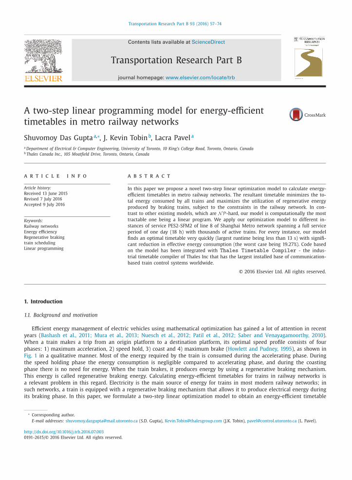
When a train makes a trip from an origin platform to a destination platform, its optimal speed profile consists of four
phases: 1) maximum acceleration, 2) speed hold, 3) coast and 4) maximum brake ( Howlett and Pudney, 1995 ), as shown in
Fig. 1 in a qualitative manner. Most of the energy required by the train is consumed during the accelerating phase. During
the speed holding phase the energy consumption is negligible compared to accelerating phase, and during the coasting
phase there is no need for energy. When the train brakes, it produces energy by using a regenerative braking mechanism.
This energy is called regenerative braking energy. Calculating energy-efficient timetables for trains in railway networks is
a relevant problem in this regard. Electricity is the main source of energy for trains in most modern railway networks; in
such networks, a train is equipped with a regenerative braking mechanism that allows it to produce electrical energy during
its braking phase. In this paper, we formulate a two-step linear optimization model to obtain an energy-efficient timetable
∗ Corresponding author.
E-mail addresses: [email protected] (S.D. Gupta), [email protected] (J.K. Tobin), [email protected] (L. Pavel).
http://dx.doi.org/10.1016/j.trb.2016.07.003
0191-2615/© 2016 Elsevier Ltd. All rights reserved.
58 S.D. Gupta et al. / Transportation Research Part B 93 (2016) 57–74
Fig. 1. Optimal speed profile of a train.
for a metro railway network. The timetable schedules the arrival time and the departure time of each train to and from the
platforms it visits such that the total electrical energy consumed is minimized and the utilization of produced regenerative
energy is maximized.
1.2. Related work
The general timetabling problem in a metro railway network has been studied extensively over the past three decades
( Harrod, 2012 ). However, very few results exist that can calculate energy-efficient timetables. Now we discuss the related
research. We classify the related work as follows. The first two papers are mixed integer programming model, the next three
are models based on meta-heuristics and the last one is an analytical study.
A Mixed Integer Programming (MIP) model, applicable only to single train-lines, is proposed by Peña-Alcaraz et al.
(2012a ) to maximize the total duration of all possible synchronization processes between all possible train pairs. The model
is then applied successfully to line three of the Madrid underground system. However, the model can have some drawbacks.
First, considering all train pairs in the objective will result in a computationally intractable problem even for a moderate
sized railway network. Second, for a train pair in which the associated trains are far apart from each other, most, if not all,
of the regenerative energy will be lost due to the transmission loss of the overhead contact line. Finally, the model assumes
that the durations of braking and accelerating phases stay the same with varying trip times, which is not the case in reality.
The work in Das Gupta et al. (2015) proposes a more tractable MIP model, applicable to any railway network, by consider-
ing only train pairs suitable for regenerative energy transfer. The optimization model is applied numerically to the Dockland
Light Railway and shows a significant increase in the total duration of the synchronization process. Although such increase,
in principle, may increase the total savings in regenerative energy, the actual energy saving is not directly addressed. Simi-
lar to Peña-Alcaraz et al. (2012a ), this model too, assumes that even if the trip time changes, the duration of the associated
braking and accelerating stay the same.
S.D. Gupta et al. / Transportation Research Part B 93 (2016) 57–74 59
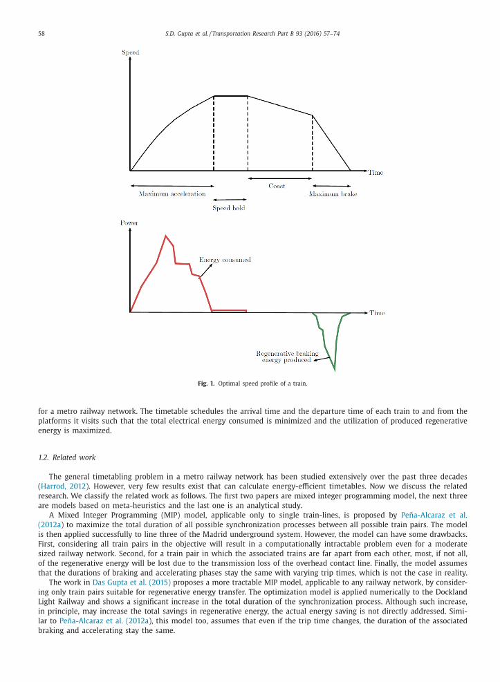
Fig. 2. Flow-chart of the two steps of the optimization model.
Other relevant works implement meta-heuristics. The work in Li and Lo (2014a ) implements genetic algorithm to cal-
culate timetables that maximize the utilization of regenerative energy while minimizing the tractive energy of the trains.
Numerical studies for the model is implemented to Beijing Metro Yizhuang Line of China showing notable increase in energy
efficiency. The work in Yang et al. (2013) presents a cooperative integer programming model to utilize the use of regener-
ative energy of trains and proposes genetic algorithm to solve it. Similar to Li and Lo (2014a ), this numerical studies have
been performed to Beijing Metro Yizhuang Line of China, though the improvement is stated in the increase in overlapping
time only. The work in Le et al. (2014) presents a nonlinear integer programming model which is solved using simulated
annealing. The numerical experiments have been conducted for the island line of the mass transit system in Hong Kong.
An insightful analytical study of a periodic railway schedule appears in Li and Lo (2014b ). The model uses the KKT condi-
tions to calculate and analyze the properties of an energy-efficient timetable. The resultant analytical model is then applied
to Beijing Metro Yizhuang Line of China numerically, which shows that the model can reduce the net energy consumption
considerably.
1.3. Contributions
We propose a novel two-step linear optimization model to calculate an energy-efficient railway timetable. The first opti-
mization model minimizes the total energy consumed by all trains subject to the constraints present in the railway network.
The problem can be formulated as a linear program, with the optimal value attained by an integral vector. The second op-
timization model uses the optimal trip time from the first optimization model and maximizes the transfer of regenerative
braking energy between suitable train pairs. Both the steps of our optimization model are linear programs, whereas the op-
timization models in related works are N P -hard. A flow-chart of the two steps of the optimization model is shown in Fig. 2 .
Our model can calculate energy-efficient railway timetables for large scale networks in a short CPU time. Code based on the
model has been embedded with the railway timetable compiler ( Thales Timetable Compiler ) of Thales Inc, which
has the largest installed base of communication-based train control systems worldwide. Thales Timetable Compileris used by many railway management systems worldwide including: Docklands Light Railway in London, UK., the West Rail
Line and Ma On Shan Line in Hong Kong, the Red Line and Green Line in Dubai, the Kelana Jaya Line in Kuala Lumpur.
This paper is organized as follows. In Section 2 we describe the notation used, and then in Section 3 we model and justify
the constraints present in the railway network. The first optimization model is presented in Section 4 . Section 5 formulates
the second optimization problem that additionally maximizes the utilization of regenerative braking energy. Section 6 de-
scribes the limitations of the optimization model. In Section 7 we apply our model to different instances of an existing
metro railway network spanning a full working day and describe the results. Section 8 presents the conclusion.
2. Notation and notions
Every set described in this paper is strictly ordered and finite unless otherwise specified. The set-cardinality (number of
elements of the set) and the i th element of such a set C is denoted by | C | and C ( i ) respectively. The set of real numbers and
integers are expressed by R and Z respectively; subscripts + and ++ attached with either set denote non-negativity and
positivity of the elements respectively. A column vector with all components one is denoted by 1 . The symbol � stands for
componentwise inequality between two vectors and the symbol ∧ stands for conjunction. The number of nonzero compo-
nents of a vector x is called cardinality of that vector and is denoted by card (x ) . Note that, cardinality of a vector is different
from set-cardinality. The i th unit vector e i is the vector with all components zero except for the i th component which is one.
The epigraph of a function f : C → R (where C is any set) denoted by epi f is the set of input-output pairs that f can achieve
along with anything above, i.e.,
epi f = { (x, t) ∈ C × R | x ∈ C, t ≥ f (x ) } . The convex hull of any set C , denoted by conv C, is the set containing all convex combinations of points in C . Consequently,
if C is nonconvex, then its best convex outer approximation is conv C, as it is the smallest set containing C .
The set of all platforms in a railway network is indicated by N . A directed arc between two distinct and non-opposite
platforms is called a track. The set of all tracks is represented by A . The directed graph of the railway network is expressed
60 S.D. Gupta et al. / Transportation Research Part B 93 (2016) 57–74
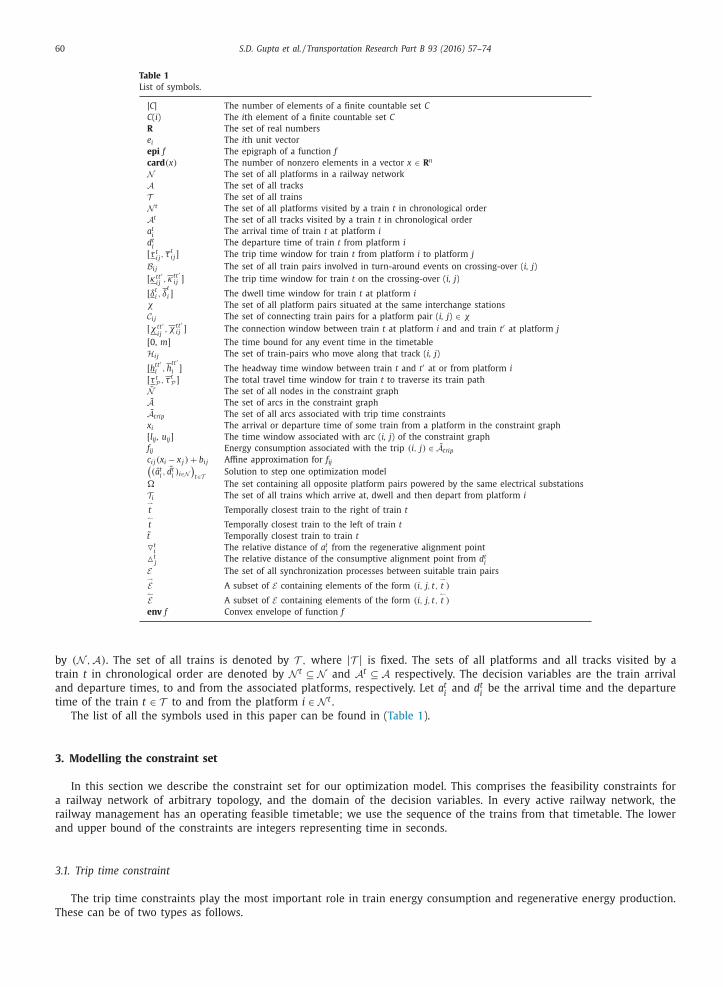
Table 1
List of symbols.
| C | The number of elements of a finite countable set C
C ( i ) The i th element of a finite countable set C
R The set of real numbers
e i The i th unit vector
epi f The epigraph of a function f
card (x ) The number of nonzero elements in a vector x ∈ R n N The set of all platforms in a railway network
A The set of all tracks
T The set of all trains
N
t The set of all platforms visited by a train t in chronological order
A
t The set of all tracks visited by a train t in chronological order
a t i
The arrival time of train t at platform i
d t i
The departure time of train t from platform i
[ τ t i j , τ t
i j ] The trip time window for train t from platform i to platform j
B i j The set of all train pairs involved in turn-around events on crossing-over ( i, j )
[ κ t t ′ i j
, κ t t ′ i j ] The trip time window for train t on the crossing-over ( i, j )
[ δt i , δ
t
i ] The dwell time window for train t at platform i
χ The set of all platform pairs situated at the same interchange stations
C i j The set of connecting train pairs for a platform pair ( i, j ) ∈ χ[ χ t t ′
i j , χ t t ′
i j ] The connection window between train t at platform i and and train t ′ at platform j
[0, m ] The time bound for any event time in the timetable
H i j The set of train-pairs who move along that track ( i, j )
[ h t t ′ i , h
t t ′ i ] The headway time window between train t and t ′ at or from platform i
[ τ t P , τ
t P ] The total travel time window for train t to traverse its train path
N The set of all nodes in the constraint graph
A The set of arcs in the constraint graph
A trip The set of all arcs associated with trip time constraints
x i The arrival or departure time of some train from a platform in the constraint graph
[ l ij , u ij ] The time window associated with arc ( i, j ) of the constraint graph
f ij Energy consumption associated with the trip (i, j) ∈ A trip
c i j (x i − x j ) + b i j Affine approximation for f ij (( a t
i , d t
i ) i ∈N
)t∈T Solution to step one optimization model
� The set containing all opposite platform pairs powered by the same electrical substations
T i The set of all trains which arrive at, dwell and then depart from platform i ⇀
t Temporally closest train to the right of train t ↼
t Temporally closest train to the left of train t ˜ t Temporally closest train to train t
� t i
The relative distance of a t i
from the regenerative alignment point
� t j
The relative distance of the consumptive alignment point from d t i
E The set of all synchronization processes between suitable train pairs ⇀
E A subset of E containing elements of the form (i, j, t, ⇀
t ) ↼
E A subset of E containing elements of the form (i, j, t, ↼
t )
env f Convex envelope of function f
by (N , A ) . The set of all trains is denoted by T , where |T | is fixed. The sets of all platforms and all tracks visited by a
train t in chronological order are denoted by N
t ⊆ N and A
t ⊆ A respectively. The decision variables are the train arrival
and departure times, to and from the associated platforms, respectively. Let a t i
and d t i
be the arrival time and the departure
time of the train t ∈ T to and from the platform i ∈ N
t .
The list of all the symbols used in this paper can be found in ( Table 1 ).
3. Modelling the constraint set
In this section we describe the constraint set for our optimization model. This comprises the feasibility constraints for
a railway network of arbitrary topology, and the domain of the decision variables. In every active railway network, the
railway management has an operating feasible timetable; we use the sequence of the trains from that timetable. The lower
and upper bound of the constraints are integers representing time in seconds.
3.1. Trip time constraint
The trip time constraints play the most important role in train energy consumption and regenerative energy production.
These can be of two types as follows.
S.D. Gupta et al. / Transportation Research Part B 93 (2016) 57–74 61
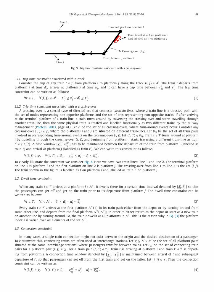
Fig. 3. Trip time constraint associated with a crossing-over.
t
3.1.1. Trip time constraint associated with a track
Consider the trip of any train t ∈ T from platform i to platform j along the track (i, j) ∈ A
t . The train t departs from
platform i at time d t i , arrives at platform j at time a t
j , and it can have a trip time between τ t
i j and τ t
i j . The trip time
constraint can be written as follows:
∀ t ∈ T , ∀ (i, j) ∈ A
t , τ t i j ≤ a t j − d t i ≤ τ t
i j . (1)
3.1.2. Trip time constraint associated with a crossing-over
A crossing-over is a special type of directed arc that connects two train-lines , where a train-line is a directed path with
the set of nodes representing non-opposite platforms and the set of arcs representing non-opposite tracks. If after arriving
at the terminal platform of a train-line, a train turns around by traversing the crossing-over and starts travelling through
another train-line, then the same physical train is treated and labelled functionally as two different trains by the railway
management ( Peeters, 2003 , page 41). Let ϕ be the set of all crossing-overs, where turn-around events occur. Consider any
crossing-over ( i, j ) ∈ ϕ, where the platforms i and j are situated on different train-lines. Let B i j be the set of all train pairs
involved in corresponding turn-around events on the crossing-over ( i, j ). Let (t , t ′ ) ∈ B i j . Train t ∈ T turns around at platform
i by travelling through the crossing-over ( i, j ), and beginning from platform j starts traversing a different train-line as train
′ ∈ T \ { t} . A time window [ κt t ′ i j
, κt t ′ i j ] has to be maintained between the departure of the train from platform i (labelled as
train t ) and arrival at platform j (labelled as train t ′ ). We can write this constraint as follows:
∀ (i, j) ∈ ϕ, ∀ (t , t ′ ) ∈ B i j , κ t t ′ i j ≤ a t
′ j − d t i ≤ κ t t ′
i j . (2)
To clearly illustrate the constraint we consider Fig. 3 . Here we have two train lines: line 1 and line 2. The terminal platform
on line 1 is platform i and the first platform on line 2 is platform j . The crossing-over from line 1 to line 2 is the arc ( i, j ).
The train shown in the figure is labelled as t on platform i and labelled as train t ′ on platform j .
3.2. Dwell time constraint
When any train t ∈ T arrives at a platform i ∈ N
t , it dwells there for a certain time interval denoted by [ δt i , δ
t
i ] so that
the passengers can get off and get on the train prior to its departure from platform j . The dwell time constraint can be
written as follows:
∀ t ∈ T , ∀ i ∈ N
t , δt i ≤ d t i − a t i ≤ δ
t
i . (3)
Every train t ∈ T arrives at the first platform N
t (1) in its train-path either from the depot or by turning around from
some other line, and departs from the final platform N
t (|N
t | ) in order to either return to the depot or start as a new train
on another line by turning around. So, the train t dwells at all platforms in N
t . This is the reason why in Eq. (3) the platform
index i is varied over all elements of the set N
t .
3.3. Connection constraint
In many cases, a single train connection might not exist between the origin and the desired destination of a passenger.
To circumvent this, connecting trains are often used at interchange stations. Let χ ⊆ N × N be the set of all platform pairs
situated at the same interchange stations, where passengers transfer between trains. Let C i j be the set of connecting train
pairs for a platform pair ( i, j ) ∈ χ . For a train pair (t , t ′ ) ∈ C i j , train t is arriving at platform i and train t ′ ∈ T is depart-
ing from platform j . A connection time window denoted by [ χ t t ′ i j
, χ t t ′ i j ] is maintained between arrival of t and subsequent
departure of t ′ , so that passengers can get off from the first train and get on the latter. Let ( i, j ) ∈ χ . Then the connection
constraint can be written as:
∀ (i, j) ∈ χ, ∀ (t , t ′ ) ∈ C , χ t t ′ ≤ d t ′ − a t ≤ χ t t ′
. (4)
i j i j j i i j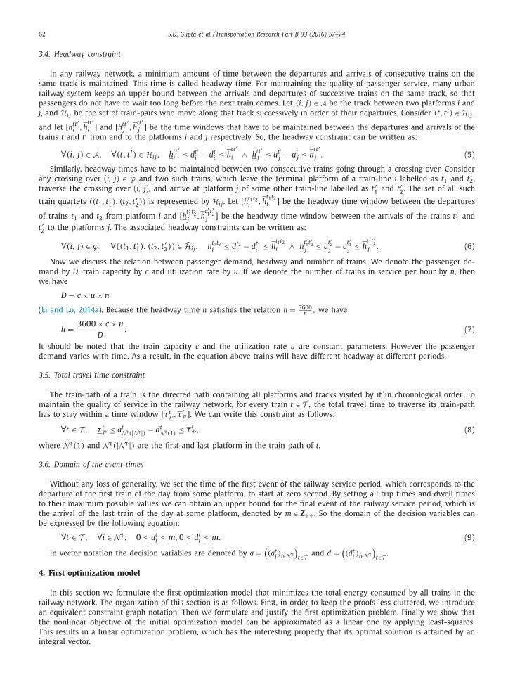
62 S.D. Gupta et al. / Transportation Research Part B 93 (2016) 57–74
3.4. Headway constraint
In any railway network, a minimum amount of time between the departures and arrivals of consecutive trains on the
same track is maintained. This time is called headway time. For maintaining the quality of passenger service, many urban
railway system keeps an upper bound between the arrivals and departures of successive trains on the same track, so that
passengers do not have to wait too long before the next train comes. Let (i, j) ∈ A be the track between two platforms i and
j , and H i j be the set of train-pairs who move along that track successively in order of their departures. Consider (t , t ′ ) ∈ H i j ,
and let [ h t t ′ i , h
t t ′ i ] and [ h
t t ′ j , h
t t ′ j ] be the time windows that have to be maintained between the departures and arrivals of the
trains t and t ′ from and to the platforms i and j respectively. So, the headway constraint can be written as:
∀ (i, j) ∈ A , ∀ (t , t ′ ) ∈ H i j , h
t t ′ i ≤ d t
′ i − d t i ≤ h
t t ′ i ∧ h
t t ′ j ≤ a t
′ j − a t j ≤ h
t t ′ j . (5)
Similarly, headway times have to be maintained between two consecutive trains going through a crossing over. Consider
any crossing over ( i, j ) ∈ ϕ and two such trains, which leave the terminal platform of a train-line i labelled as t 1 and t 2 ,
traverse the crossing over ( i, j ), and arrive at platform j of some other train-line labelled as t ′ 1
and t ′ 2 . The set of all such
train quartets ((t 1 , t ′ 1 ) , (t 2 , t
′ 2 )) is represented by ˜ H i j . Let [ h
t 1 t 2 i
, h t 1 t 2 i ] be the headway time window between the departures
of trains t 1 and t 2 from platform i and [ h t ′ 1
t ′ 2
j , h
t ′ 1
t ′ 2
j ] be the headway time window between the arrivals of the trains t ′ 1
and
t ′ 2
to the platforms j . The associated headway constraints can be written as:
∀ (i, j) ∈ ϕ, ∀ ((t 1 , t ′ 1 ) , (t 2 , t
′ 2 )) ∈
˜ H i j , h
t 1 t 2 i ≤ d t 2
i − d t 1
i ≤ h
t 1 t 2
i ∧ h
t ′ 1 t ′ 2 j
≤ a t ′ 2 j
− a t ′ 1 j
≤ h
t ′ 1 t ′ 2 j . (6)
Now we discuss the relation between passenger demand, headway and number of trains. We denote the passenger de-
mand by D , train capacity by c and utilization rate by u . If we denote the number of trains in service per hour by n , then
we have
D = c × u × n
( Li and Lo, 2014a ). Because the headway time h satisfies the relation h =
3600 n , we have
h =
3600 × c × u
D
. (7)
It should be noted that the train capacity c and the utilization rate u are constant parameters. However the passenger
demand varies with time. As a result, in the equation above trains will have different headway at different periods.
3.5. Total travel time constraint
The train-path of a train is the directed path containing all platforms and tracks visited by it in chronological order. To
maintain the quality of service in the railway network, for every train t ∈ T , the total travel time to traverse its train-path
has to stay within a time window [ τ t P , τ
t P ] . We can write this constraint as follows:
∀ t ∈ T , τ t P ≤ a t N t (|N t | ) − d t N t (1) ≤ τ t
P , (8)
where N
t (1) and N
t (|N
t | ) are the first and last platform in the train-path of t .
3.6. Domain of the event times
Without any loss of generality, we set the time of the first event of the railway service period, which corresponds to the
departure of the first train of the day from some platform, to start at zero second. By setting all trip times and dwell times
to their maximum possible values we can obtain an upper bound for the final event of the railway service period, which is
the arrival of the last train of the day at some platform, denoted by m ∈ Z ++ . So the domain of the decision variables can
be expressed by the following equation:
∀ t ∈ T , ∀ i ∈ N
t , 0 ≤ a t i ≤ m, 0 ≤ d t i ≤ m. (9)
In vector notation the decision variables are denoted by a =
((a t
i ) i ∈N t
)t∈T and d =
((d t
i ) i ∈N t
)t∈T .
4. First optimization model
In this section we formulate the first optimization model that minimizes the total energy consumed by all trains in the
railway network. The organization of this section is as follows. First, in order to keep the proofs less cluttered, we introduce
an equivalent constraint graph notation. Then we formulate and justify the first optimization problem. Finally we show that
the nonlinear objective of the initial optimization model can be approximated as a linear one by applying least-squares.
This results in a linear optimization problem, which has the interesting property that its optimal solution is attained by an
integral vector.
S.D. Gupta et al. / Transportation Research Part B 93 (2016) 57–74 63
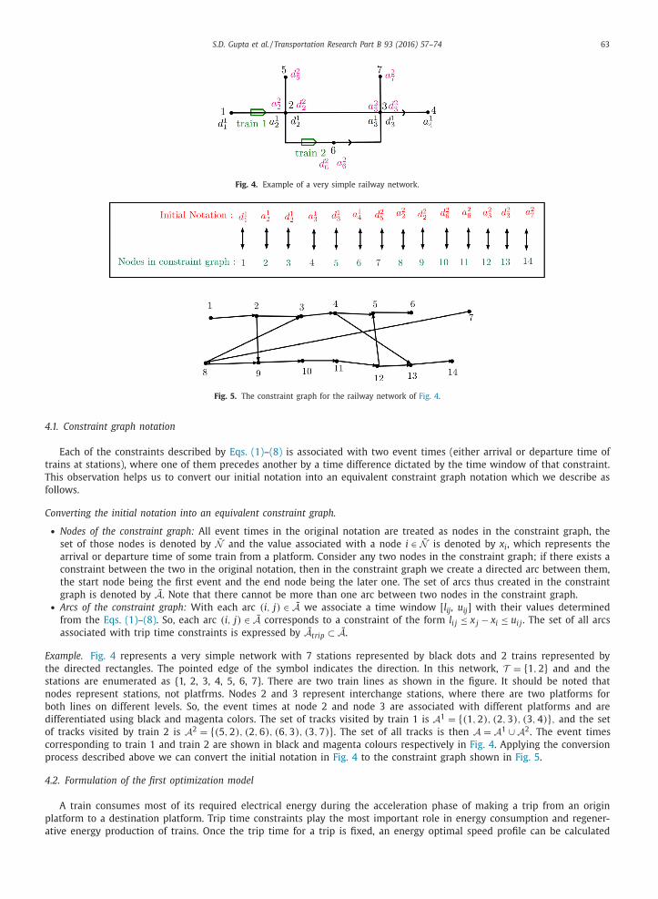
Fig. 4. Example of a very simple railway network.
Fig. 5. The constraint graph for the railway network of Fig. 4 .
4.1. Constraint graph notation
Each of the constraints described by Eqs. (1) –(8) is associated with two event times (either arrival or departure time of
trains at stations), where one of them precedes another by a time difference dictated by the time window of that constraint.
This observation helps us to convert our initial notation into an equivalent constraint graph notation which we describe as
follows.
Converting the initial notation into an equivalent constraint graph.
• Nodes of the constraint graph: All event times in the original notation are treated as nodes in the constraint graph, the
set of those nodes is denoted by N and the value associated with a node i ∈ N is denoted by x i , which represents the
arrival or departure time of some train from a platform. Consider any two nodes in the constraint graph; if there exists a
constraint between the two in the original notation, then in the constraint graph we create a directed arc between them,
the start node being the first event and the end node being the later one. The set of arcs thus created in the constraint
graph is denoted by A . Note that there cannot be more than one arc between two nodes in the constraint graph. • Arcs of the constraint graph: With each arc (i, j) ∈ A we associate a time window [ l ij , u ij ] with their values determined
from the Eqs. (1) –(8) . So, each arc (i, j) ∈ A corresponds to a constraint of the form l i j ≤ x j − x i ≤ u i j . The set of all arcs
associated with trip time constraints is expressed by A trip ⊂ A .
Example. Fig. 4 represents a very simple network with 7 stations represented by black dots and 2 trains represented by
the directed rectangles. The pointed edge of the symbol indicates the direction. In this network, T = { 1 , 2 } and and the
stations are enumerated as {1, 2, 3, 4, 5, 6, 7}. There are two train lines as shown in the figure. It should be noted that
nodes represent stations, not platfrms. Nodes 2 and 3 represent interchange stations, where there are two platforms for
both lines on different levels. So, the event times at node 2 and node 3 are associated with different platforms and are
differentiated using black and magenta colors. The set of tracks visited by train 1 is A
1 = { (1 , 2) , (2 , 3) , (3 , 4) } , and the set
of tracks visited by train 2 is A
2 = { (5 , 2) , (2 , 6) , (6 , 3) , (3 , 7) } . The set of all tracks is then A = A
1 ∪ A
2 . The event times
corresponding to train 1 and train 2 are shown in black and magenta colours respectively in Fig. 4 . Applying the conversion
process described above we can convert the initial notation in Fig. 4 to the constraint graph shown in Fig. 5 .
4.2. Formulation of the first optimization model
A train consumes most of its required electrical energy during the acceleration phase of making a trip from an origin
platform to a destination platform. Trip time constraints play the most important role in energy consumption and regener-
ative energy production of trains. Once the trip time for a trip is fixed, an energy optimal speed profile can be calculated
64 S.D. Gupta et al. / Transportation Research Part B 93 (2016) 57–74
efficiently by existing software ( Vlad and Tatarnikov, 2011 ), ( Howlett and Pudney, 1995 , page 285), such as Thales T rain
K inetics, D ynamics and C ontrol (TKDC) Simulator in our case. The TKDC simulator assumes maximum accelerating - speed
holding - coasting - maximum braking strategy for calculation of speed profile. Theoretically this is the optimal speed profile
according to the monograph ( Howlett and Pudney, 1995 ). For calculation of the optimal speed profile of a train while mak-
ing a trip, we refer the interested reader to the highly cited papers ( Howlett, 20 0 0; Howlett et al., 2009; Jiaxin and Howlett,
1993; Khmelnitsky, 20 0 0; Liu and Golovitcher, 2003 ). An excellent state-of-the art review of calculating energy-efficient or
energy-optimal speed profile can be found in Albrecht et al. (2015) . The key assumptions that we have made in calculating
the speed profiles, all of which are well-established in relevant literature ( Albrecht et al., 2015 ), are as follows.
• The acceleration and braking control forces are assumed to be uniformly bounded or bounded by magnitude constraints.
These magnitude constraints are assumed to be dependent on the speed of the train and non-increasing. • The initial speed of the train from the origin platform and final speed at the destination platform are assumed to be
zero. The speed is assumed to be strictly positive at every other position. • Only the force associated with positive acceleration consumes energy. • The rate of energy dissipation from frictional resistance is assumed to be a quadratic function of the form a 0 + a 1 v + a 2 v 2
(also known as the Davis formula ( Davis, 1926 )), where v stands for speed of the train and a 0 , a 1 , a 2 are non-negative
physical constants. These constants can be determined approximately in practice by measuring the difference between
the applied tractive force and the net tractive force. • We have assumed the position of the train to be an independent variable and speed of the train to be a dependent vari-
able. This assumption appears all the major contributions. This assumption appears all the major contributions. A notable
exception is Khmelnitsky (20 0 0) , which considers kinetic energy and time as the dependent variables and position as the
independent variable.
The electrical power consumption and regeneration of a train on a track is determined by its speed profile, so the optimal
speed profile also gives the power versus time graph ( power graph in short) for that trip. However, in the total railway
service period there are many active trains, whose movements are coupled by the associated constraints. So, finding the
energy-minimal trip time for a single trip in an isolated manner can result in a infeasible timetable. Consider an arc (i, j) ∈A trip in the constraint graph, associated with some trip time constraint. Let us denote the energy consumption function for
that trip f i j : R ++ → R ++ with argument (x j − x i ) . The first optimization problem with the objective to minimize the total
energy consumption of the trains can be written as:
minimize ∑
(i, j) ∈ A trip f i j (x j − x i )
subject to l i j ≤ x j − x i ≤ u i j , ∀ (i, j) ∈ A
0 ≤ x i ≤ m, ∀ i ∈ N ,
(10)
where the decision vector is (x i ) i ∈ N ∈ R
| N | . The exact analytical form of every component of the objective function, i.e. , f i j (x j − x i ) for (i, j) ∈ A trip is not known and
may be intractable ( Howlett et al., 2009 ). However, irrespective of the exact analytical form, the energy function can be
shown to be monotonically decreasing in trip time, i.e. , it is non-increasing with the increase in trip time, if the optimal
speed profile is followed ( Milroy, 1980 ). Even when a train is manually driven with possibly suboptimal driving strategies,
the average energy consumption of the train is found empirically to be monotonically decreasing in the trip time ( Peña-
Alcaraz et al., 2012b ).
Also, the energy function is relatively easy to measure in practice ( Howlett and Pudney, 1995 , Section 1.5). For any
(i, j) ∈ A trip , we denote the measured trip times (x (1) j
− x (1) i
) , . . . , (x (p) j
− x (p) i
) and the corresponding energy consumption
data f (1) i j
, . . . , f (p) i j
.
In any subway system, the amount by which the trip time is allowed to vary in Eqs. (1) and (2) is typically on the order
of seconds ( Liebchen, 2007 ), which motivates us to make the following assumption.
Assumption 1. The amount by which the trip time is allowed to vary is on the order of seconds, i.e., for any the trip time
window is on the order of seconds.
The monotonically decreasing nature of the energy function together with Assumption 1 allows us to approximate the
energy function f i j (x j − x i ) as an affine function. Recall that in practice, we can measure the energy f (1) i j
, . . . , f (p) i j
and as-
sociated trip times (x (1) j
− x (1) i
) , . . . , (x (p) j
− x (p) i
) , which is obtainable easily with present technology ( Howlett and Pudney,
1995 , Section 1.5).
Now we want to formulate an optimization problem which will provide us with the best possible affine approximation of
the energy function f i j (x j − x i ) . We do so by applying least-squares and fit a straight line through measured energy versus
trip time data. We seek an affine function c i j (x j − x i ) + b i j = (x j − x i , 1) T (c i j , b i j ) where we want to determine c ij and b ij .
S.D. Gupta et al. / Transportation Research Part B 93 (2016) 57–74 65
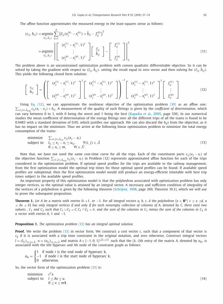
The affine function approximates the measured energy in the least-squares sense as follows:
(c i j , b i j ) = argmin
( c i j , b i j )
p ∑
k =1
(˜ c i j (x (k )
j − x (k )
i ) +
b i j − f (k ) i j
)2
= argmin
( c i j , b i j )
∥∥∥∥∥∥∥⎡
⎢ ⎣
(x (1) j
− x (1) i
, 1) T
. . .
(x (p) j
− x (p) i
, 1) T
⎤
⎥ ⎦
[˜ c i j
˜ b i j
]−
⎡
⎢ ⎣
f (1) i j
. . .
f (p) i j
⎤
⎥ ⎦
∥∥∥∥∥∥∥2
2
(11)
The problem above is an unconstrained optimization problem with convex quadratic differentiable objective. So it can be
solved by taking the gradient with respect to ( c i j , b i j ) , setting the result equal to zero vector and then solving for ( c i j ,
b i j ) .
This yields the following closed form solution:
[c i j
b i j
]=
⎛
⎜ ⎜ ⎝
⎡
⎢ ⎣
(x (1) j
− x (1) i
, 1) T
. . .
(x (p) j
− x (p) i
, 1) T
⎤
⎥ ⎦
T ⎡
⎢ ⎣
(x (1) j
− x (1) i
, 1) T
. . .
(x (p) j
− x (p) i
, 1) T
⎤
⎥ ⎦
⎞
⎟ ⎟ ⎠
−1 ⎡
⎢ ⎣
(x (1) j
− x (1) i
, 1) T
. . .
(x (p) j
− x (p) i
, 1) T
⎤
⎥ ⎦
T ⎡
⎢ ⎣
f (1) i j
. . .
f (p) i j
⎤
⎥ ⎦
(12)
Using Eq. (12) , we can approximate the nonlinear objective of the optimization problem (10) as an affine one:∑
(i, j) ∈ A trip c i j (x i − x j ) + b i j . A measurement of the quality of such fittings is given by the coefficient of determination , which
can vary between 0 to 1, with 0 being the worst and 1 being the best ( Kapadia et al., 2005 , page 518). In our numerical
studies the mean coefficient of determination of the energy fittings over all the different trips of all the trains is found to be
0.9483 with a standard deviation of 0.05, which justifies our approach. We can also discard the b ij s from the objective, as it
has no impact on the minimizer. Thus we arrive at the following linear optimization problem to minimize the total energy
consumption of the trains:
minimize ∑
(i, j) ∈ A trip c i j (x j − x i )
subject to l i j ≤ x j − x i ≤ u i j , ∀ (i, j) ∈ A
0 ≤ x i ≤ m, ∀ i ∈ N .
(13)
Note that, we have not used the same cost-time curve for all the trips. Each of the constituent parts c i j (x j − x i ) of
the objective function
∑
(i, j) ∈ A trip c i j (x j − x i ) in Problem (12) represents approximated affine function for each of the trips
considered in the optimization problem. If optimal speed profiles for the trips are available to the railway management,
from the first optimization model the optimal trip times for those optimal speed profiles can be found. If available speed
profiles are suboptimal, then the first optimization model would still produce an energy-efficient timetable with best trip
times subject to the available speed profiles.
An important property of this optimization model is that the polyhedron associated with optimization problem has only
integer vertices, so the optimal value is attained by an integral vector. A necessary and sufficient condition of integrality of
the vertices of a polyhedron is given by the following theorem ( Schrijver, 1998 , page 269, Theorem 19.3), which we will use
to prove the subsequent proposition.
Theorem 1. Let A be a matrix with entries 0 , +1 , or −1 . For all integral vectors a, b, c, d the polyhedron { x ∈ R
n | c � x �d, a
� Ax � b } has only integral vertices if and only if for each nonempty collection of columns of A, denoted by C, there exist two
subsets , C 1 and C 2 such that C 1 ∪ C 2 = C, C 1 ∩ C 2 = ∅ , and the sum of the columns in C 1 minus the sum of the columns in C 2 is
a vector with entries 0, 1 and −1 .
Proposition 1. The optimization problem (13) has an integral optimal solution.
Proof. We write the problem (13) in vector form. We construct a cost vector c , such that a component of that vector is
c ij if it is associated with a trip time constraint in the original notation, and zero otherwise. Construct integral vectors
l = (l i j ) (i, j) ∈ A , u = (u i j ) (i, j) ∈ A and matrix A ∈ {−1 , 0 , 1 } | A |×| N | such that the ( k, i )th entry of the matrix A , denoted by a ki , is
associated with the k th hyperarc and i th node of the constraint graph as follows:
a ki =
{
1 if node i is the end node of hyperarc k, −1 if node i is the start node of hyperarc k, 0 otherwise.
So, the vector form of the optimization problem (13) is:
minimize c T x subject to l � Ax � u,
0 � x � m 1 .
(14)
66 S.D. Gupta et al. / Transportation Research Part B 93 (2016) 57–74
Consider any nonempty collection of columns of A denoted by C . Take C 1 = C and C 2 = ∅ . Then the sum of the columns in C 1 minus the sum of the columns in C 2 will be a vector with entries 0, 1 and −1 , because in A there cannot exist more than
one row corresponding to an arc between two nodes of the constraint graph and each such row has exactly two nonzero
entries, a +1 and a −1 . So, by Theorem 1 the polyhedron { x ∈ R
| N | : l � Ax � u, 0 � x � m 1 } has only integral vertices and
optimizing the linear objective in problem (14) over this polyhedron will result in an integral solution. �
After solving the linear programming problem (13) , we obtain an integral timetable, which we will call the energy mini-
mizing timetable ( EMT ). We denote the optimal decision vector of this timetable by x in the constraint graph notation and(( a t
i , d t
i ) i ∈N
)t∈T in the original notation.
5. Second optimization model
In this section we modify the trip time constraints such that the total energy consumption of the final timetable is
kept at the same minimum as the EMT. Then, we describe our optimization strategy aimed to maximize the utilization of
regenerative energy of braking trains, and we present the second optimization model.
5.1. Keeping the total energy consumption at minimum
In any feasible timetable, if the trip times are kept to be the same as the ones obtained from the EMT, then the energy
optimal speed profiles for all trains will be the same. As a result, the energy consumption associated with that timetable
will remain at the same minimum as found in the EMT. So, in the second optimization problem, instead of using the trip
time constraint, for every trip we fix the trip time to the value in the EMT, i.e.,
∀ t ∈ T , ∀ (i, j) ∈ A
t , a t j − d t i = a t j − d t i , (15)
and
∀ (i, j) ∈ ϕ, ∀ (t , t ′ ) ∈ B i j , a t ′
j − d t i = a t ′
j − d t i . (16)
For all other constraints, bounds are allowed to vary as described by Eqs. (3) –(8) . As a consequence of fixing all trip times,
the power graph of every trip made by any train becomes known to us, since it depends on the corresponding optimal speed
profile calculated in real-time by existing software ( Vlad and Tatarnikov, 2011 ), ( Howlett and Pudney, 1995 , page 285).
5.2. Maximizing the utilization of regenerative energy of braking trains
In this subsection we describe our strategy to maximize the utilization of the regenerative energy produced by the
braking trains. Strategies based on transfer of regenerative braking energy back to the electrical grid requires specialized
technology such as reversible electrical substations ( González-Gil et al., 2013 ). A strategy based on storing is not feasible
with present technology, because storage options such as super-capacitors, fly-wheels, e.t.c. , have drastic discharge rates
besides being too expensive ( Avinash Balakrishnan, 2014 , page 66), ( Droste-Franke et al., 2012 , page 92). A better strategy
that can be used with existing technology ( Ciccarelli et al., 2014 ) is to transfer the regenerative energy of a braking train to
a nearby and simultaneously accelerating train, if both of them operate under the same electrical substation. We call such
pairs of trains suitable train pairs . So our objective is to maximize the total overlapped area between the graphs of power
consumption and regeneration of all suitable train pairs. To model this mathematically, we are faced with the following
tasks: i) define suitable train pairs, ii) provide a tractable description of the overlapped area between power graphs of such
a pair. We describe them as follows.
5.2.1. Defining suitable train pairs
We consider platform pairs who are opposite to each other and are powered by the same electrical substations. Thus, the
transmission loss in transferring electrical energy between them is negligible. In our work we The set containing all such
platform pairs is denoted by �. Consider any such platform pair ( i, j ) ∈ �, and let T i ⊆ T be the set of all trains which arrive
at, dwell and then depart from platform i . Suppose, t ∈ T i . Now, we are interested in finding another train
˜ t on platform j,
i.e. , ˜ t ∈ T j , which along with t would form a suitable pair for the transfer of regenerative braking energy. To achieve this, we
use the EMT. Among all trains going through platform j , the one which is temporally closest to t in the energy-minimizing
timetable is be the best candidate to form a pair with t . The temporal proximity can be of two types with respect to t ,
which results in the following definitions.
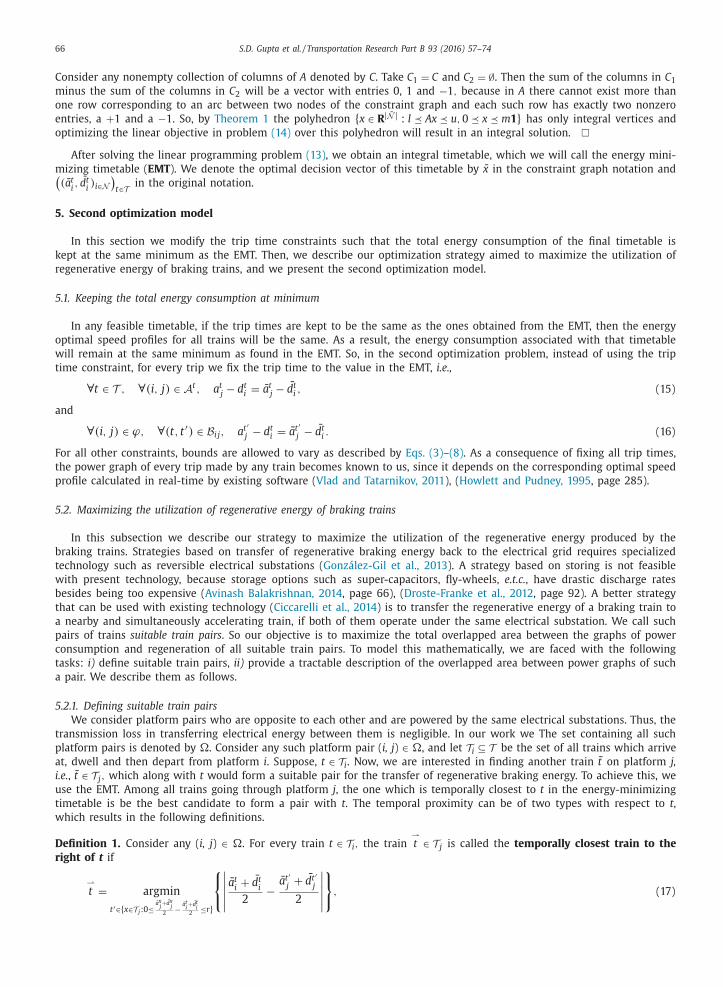
Definition 1. Consider any ( i, j ) ∈ �. For every train t ∈ T i , the train
⇀
t ∈ T j is called the temporally closest train to the
right of t if
⇀
t = argmin
t ′ ∈{ x ∈T j :0 ≤a x
j + d x
j 2 − a t
i + d t
i 2 ≤r}
{
∣∣∣∣∣ a t i + d t
i
2
−a t
′ j
+ d t ′
j
2
∣∣∣∣∣}
, (17)
S.D. Gupta et al. / Transportation Research Part B 93 (2016) 57–74 67
where r is an empirical parameter determined by the timetable designer and is much smaller than the time horizon of the
entire timetable.
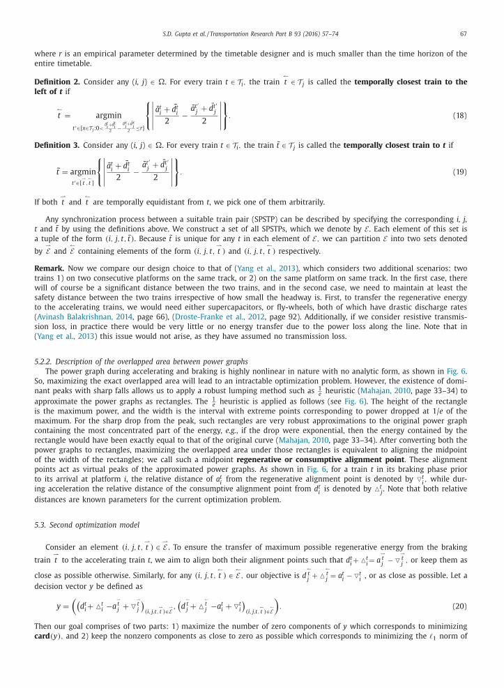
Definition 2. Consider any ( i, j ) ∈ �. For every train t ∈ T i , the train
↼
t ∈ T j is called the temporally closest train to the
left of t if
↼
t = argmin
t ′ ∈{ x ∈T j :0 < a t i + d t
i 2 −
a x j + d x
j 2 ≤r}
{
∣∣∣∣∣ a t i + d t
i
2
−a t
′ j
+ d t ′
j
2
∣∣∣∣∣}
. (18)
Definition 3. Consider any ( i, j ) ∈ �. For every train t ∈ T i , the train
˜ t ∈ T j is called the temporally closest train to t if
˜ t = argmin
t ′ ∈{ ⇀ t , ↼
t }
{
∣∣∣∣∣ a t i + d t
i
2
−a t
′ j
+ d t ′
j
2
∣∣∣∣∣}
. (19)
If both
⇀
t and
↼
t are temporally equidistant from t , we pick one of them arbitrarily.
Any synchronization process between a suitable train pair (SPSTP) can be described by specifying the corresponding i, j,
t and
˜ t by using the definitions above. We construct a set of all SPSTPs, which we denote by E . Each element of this set is
a tuple of the form (i, j, t, t ) . Because ˜ t is unique for any t in each element of E, we can partition E into two sets denoted
by ⇀
E and
↼
E containing elements of the form (i, j, t, ⇀
t ) and (i, j, t, ↼
t ) respectively.
Remark. Now we compare our design choice to that of ( Yang et al., 2013 ), which considers two additional scenarios: two
trains 1) on two consecutive platforms on the same track, or 2) on the same platform on same track. In the first case, there
will of course be a significant distance between the two trains, and in the second case, we need to maintain at least the
safety distance between the two trains irrespective of how small the headway is. First, to transfer the regenerative energy
to the accelerating trains, we would need either supercapacitors, or fly-wheels, both of which have drastic discharge rates
( Avinash Balakrishnan, 2014 , page 66), ( Droste-Franke et al., 2012 , page 92). Additionally, if we consider resistive transmis-
sion loss, in practice there would be very little or no energy transfer due to the power loss along the line. Note that in
( Yang et al., 2013 ) this issue would not arise, as they have assumed no transmission loss.
5.2.2. Description of the overlapped area between power graphs
The power graph during accelerating and braking is highly nonlinear in nature with no analytic form, as shown in Fig. 6 .
So, maximizing the exact overlapped area will lead to an intractable optimization problem. However, the existence of domi-
nant peaks with sharp falls allows us to apply a robust lumping method such as 1 e heuristic ( Mahajan, 2010 , page 33–34) to
approximate the power graphs as rectangles. The 1 e heuristic is applied as follows (see Fig. 6 ). The height of the rectangle
is the maximum power, and the width is the interval with extreme points corresponding to power dropped at 1/ e of the
maximum. For the sharp drop from the peak, such rectangles are very robust approximations to the original power graph
containing the most concentrated part of the energy, e.g. , if the drop were exponential, then the energy contained by the
rectangle would have been exactly equal to that of the original curve ( Mahajan, 2010 , page 33–34). After converting both the
power graphs to rectangles, maximizing the overlapped area under those rectangles is equivalent to aligning the midpoint
of the width of the rectangles; we call such a midpoint regenerative or consumptive alignment point . These alignment
points act as virtual peaks of the approximated power graphs. As shown in Fig. 6 , for a train t in its braking phase prior
to its arrival at platform i , the relative distance of a t i
from the regenerative alignment point is denoted by �
t i , while dur-
ing acceleration the relative distance of the consumptive alignment point from d t i
is denoted by �
t j . Note that both relative
distances are known parameters for the current optimization problem.
5.3. Second optimization model
Consider an element (i, j, t, ⇀
t ) ∈
⇀
E . To ensure the transfer of maximum possible regenerative energy from the braking
train
⇀
t to the accelerating train t , we aim to align both their alignment points such that d t i + �
t i = a
⇀
t j
− �
⇀
t j , or keep them as
close as possible otherwise. Similarly, for any (i, j, t, ↼
t ) ∈
↼
E , our objective is d ↼
t j + �
↼
t j = a t
i − �
t i
, or as close as possible. Let a
decision vector y be defined as
y =
((d t i + �
t i −a
⇀
t j + �
⇀
t j
)(i, j,t,
⇀
t ) ∈ ⇀
E , (d
↼
t j + �
↼
t j −a t i + �
t i
)(i, j,t,
↼
t ) ∈ ↼
E
). (20)
Then our goal comprises of two parts: 1) maximize the number of zero components of y which corresponds to minimizing
card (y ) , and 2) keep the nonzero components as close to zero as possible which corresponds to minimizing the norm of
1
68 S.D. Gupta et al. / Transportation Research Part B 93 (2016) 57–74
Fig. 6. Applying 1 e
heuristic to power graphs.
y , ‖ y ‖ 1 . Combining these two we can write the exact optimization problem as follows:
minimize card (y ) + γ ‖ y ‖ 1
subject to
Eq. (3)–(8),(15),(16),(20) , 0 ≤ a t
i ≤ m, 0 ≤ d t
i ≤ m, ∀ i ∈ N
t , ∀ t ∈ T ,
(21)
where γ is a positive weight, and decision variables are a, d and y . The objective function is nonconvex as shown next. Take
the convex combination of the vectors 2 e 1 / γ and 0 with convex coefficients 1/2. Then,
card
(e 1 γ
)+ γ
∥∥∥∥e 1 γ
∥∥∥∥1
= 2 >
1
2
(card
(2 e 1 γ
)+ γ
∥∥∥∥2 e 1 γ
∥∥∥∥1
)+
1
2
( card ( 0 ) + γ ‖
0 ‖ 1 ) = 1 . 5 ,
and thus violates definition of a convex function. As a result, problem (21) is a nonconvex problem. Note that if we re-
move the cardinality part from the objective, then it reduces to a convex optimization problem because the constraints are
affine and the objective is the 1 norm of an affine transformation of the decision variables ( Boyd and Vandenberghe, 2009 ,
pages 72, 79, 136–137). Such problems are often called convex-cardinality problem and are of N P -hard computational com-
plexity in general ( Calafiore and El Ghaoui, 2014 ). An effective yet tractable numerical scheme to achieve a low-cardinality
solution in a convex-cardinality problem is the 1 norm heuristic, where card (y ) is replaced by ‖ y ‖ 1 , thus converting prob-
lem (21) into a convex optimization problem. This is described by problem (22) below. The 1 norm heuristic is supported
by extensive numerical evidence with successful applications to many fields, e.g. , robust estimation in statistics, support
vector machine in machine learning, total variation reconstruction in signal processing, compressed sensing etc . In the next
section we show that in our problem too, the 1 norm heuristic produces excellent results. Intuitively, the 1 norm heuristic
works well, because it encourages sparsity in its arguments by incentivizing exact alignment between regenerative alignment
points with the associated consumptive ones ( Boyd and Vandenberghe, 20 09 , pages 30 0–301). We provide a theoretical jus-
tification for the use of 1 norm in our case as follows.
Proposition 2. The convex optimization problem described by
minimize ‖ y ‖ 1
subject to
Eq. (3)-(8),(15),(16),(20) , 0 ≤ a t
i ≤ m, 0 ≤ d t
i ≤ m, ∀ i ∈ N
t , ∀ t ∈ T ,
(22)
is the best convex approximation of the nonconvex problem (21) from below.
S.D. Gupta et al. / Transportation Research Part B 93 (2016) 57–74 69
Proof. Both problems (22) and (21) have the same constraint set, so we need to focus on the objective only. The best convex
approximation of a nonconvex function f : C → R (where C is any set) from below is given by its convex envelope env f on
C . The function env f is the largest convex function that is an under estimator of f on C, i.e.,
env f = sup { f : C → R | ˜ f is convex and
˜ f ≤ f } , where sup stands for the supremum, , the least upper bound of the set. The definition implies, epi env f = conv epi f .
From Eq. (20) we see that y is an affine transformation of a and d , and from the last constraints of problem (21) we
see that both a and d are upper bounded by m, i.e. , ‖ a ‖ ∞
≤ m and ‖ d ‖ ∞
≤ m . So there exists a positive number P such
that ‖ y ‖ ∞
≤ P . As the domain of y is bounded in an ∞
ball with radius P , env card (y ) =
1 P ‖ y ‖ 1 ( Calafiore and El Ghaoui,
2014 , page 321). So, the best convex approximation of the objective from below is 1 P ‖ y ‖ 1 + γ ‖ y ‖ 1 = ( 1 P + γ ) ‖ y ‖ 1 . As the
coefficient ( 1 P + γ ) is a constant for a particular optimization problem, it can be omitted, and thus we arrive at the claim. �
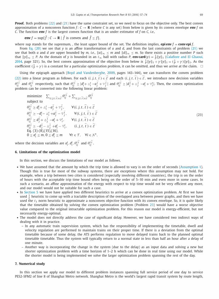
Using the epigraph approach ( Boyd and Vandenberghe, 2009 , pages 143–144), we can transform the convex problem
(22) into a linear program as follows. For each (i, j, t, ⇀
t ) ∈
⇀
E and each (i, j, t, ↼
t ) ∈
↼
E , we introduce new decision variables
θ t ⇀
t i j
and θ t ↼
t i j
respectively, such that θ t ⇀
t i j
≥ | d t i + �
t i −a
⇀
t j
+ �
⇀
t j | and θ t
↼
t i j
≥ | d ↼
t j + �
↼
t j
−a t i + �
t i | . Then, the convex optimization
problem can be converted into the following linear problem:
minimize ∑
(i, j,t, ⇀
t ) ∈ ⇀
E θ t
⇀
t i j
+
∑
(i, j,t, ↼
t ) ∈ ↼
E θ t
↼
t i j
subject to
θ t ⇀
t i j
≥ d t i + �
t i −a
⇀
t j
+ �
⇀
t j , ∀ (i, j, t,
⇀
t ) ∈
⇀
E
θ t ⇀
t i j
≥ −d t i − �
t i + a
⇀
t j
− �
⇀
t j , ∀ (i, j, t,
⇀
t ) ∈
⇀
E
θ t ↼
t i j
≥ d ↼
t j + �
↼
t j
−a t i + �
t i , ∀ (i, j, t,
↼
t ) ∈
↼
E
θ t ↼
t i j
≥ −d ↼
t j − �
↼
t j
+ a t i − �
t i , (i, j, t,
↼
t ) ∈
↼
E Eq. (3)-(8),(15),(16) , 0 ≤ a t
i ≤ m, 0 ≤ d t
i ≤ m ∀ t ∈ T , ∀ i ∈ N
t ,
(23)
where the decision variables are a t i , d t
i , θ t
⇀
t i j
and θ t ↼
t i j
.
6. Limitations of the optimization model
In this section, we discuss the limitations of our model as follows.
• We have assumed that the amount by which the trip time is allowed to vary is on the order of seconds ( Assumption 1 ).
Though this is true for most of the subway systems, there are exceptions where this assumption may not hold. For
example, when a trip between two cities is considered (especially involving different countries), the trip is on the order
of hours with the acceptable trip time bound often being on the order of 5–10 min and even more in some cases. In
such a scenario, an affine approximation of the energy with respect to trip time would not be very efficient any more,
and our model would not be suitable for such a case. • In Section 5 we have have applied two different heuristics to arrive at a convex optimization problem. At first we have
used
1 e heuristic to come up with a tractable description of the overlapped area between power graphs, and then we have
used the 1 norm heuristic to approximate a nonconvex objective function with its convex envelope. So, it is quite likely
that the timetable obtained by solving the convex optimization problem (Problem 23 ) would have a worse objective
value compared to the original intractable optimization problem. For this reason our model is energy-efficient, but not
necessarily energy-optimal. • The model does not directly address the case of significant delay. However, we have considered two indirect ways of
dealing with it in practice.
– In any automatic train supervision system, which has the responsibility of implementing the timetable, dwell and
velocity regulation are performed to maintain trains on their proper time. If there is a deviation from the optimal
timetable because of some delay, the ATS performs regulation to move delayed trains back to the planned optimal
timetable timetable. Thus the system will typically return to a normal state in less than half an hour after a delay of
one minute.
– Another way is incorporating the change in the system (due to the delay) as an input data and solving a new but
shorter optimization problem with a time horizon of 1–2 h which can be done in real time using our model. While
the shorter model is being implemented we solve the larger optimization problem spanning the rest of the day.
7. Numerical study
In this section we apply our model to different problem instances spanning full service period of one day to service
PES2-SFM2 of line 8 of Shanghai Metro network. Shanghai Metro is the world’s largest rapid transit system by route length,
70 S.D. Gupta et al. / Transportation Research Part B 93 (2016) 57–74
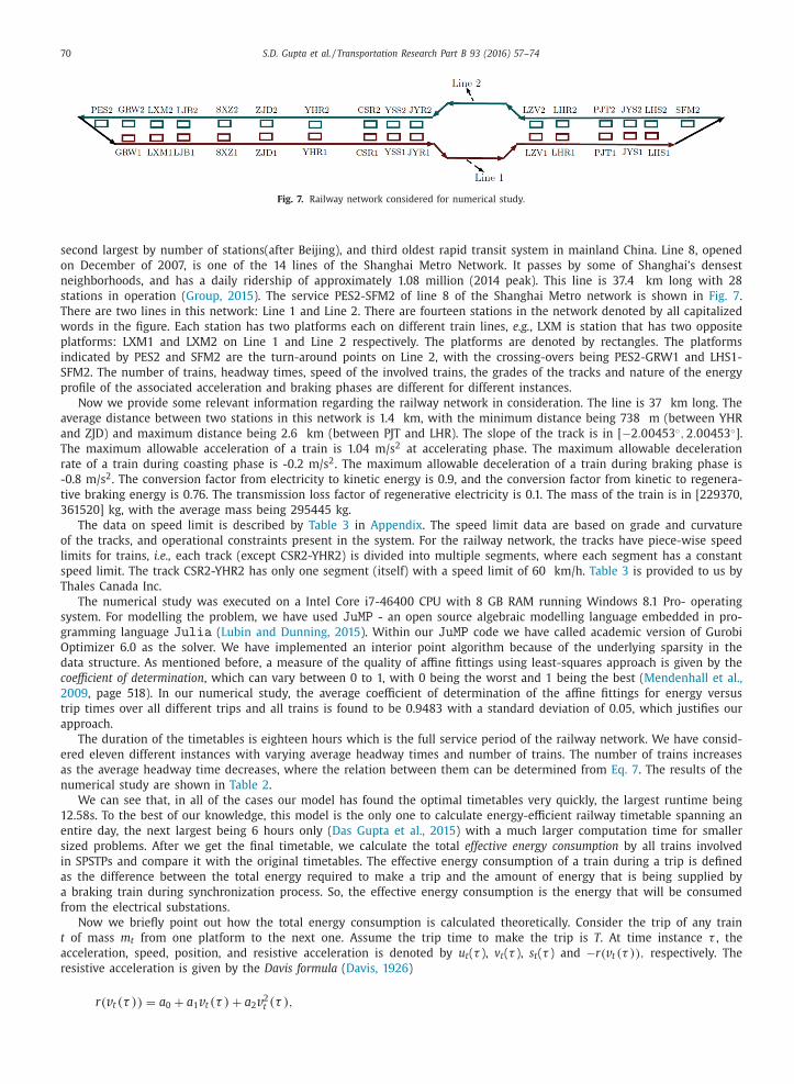
Fig. 7. Railway network considered for numerical study.
second largest by number of stations(after Beijing), and third oldest rapid transit system in mainland China. Line 8, opened
on December of 2007, is one of the 14 lines of the Shanghai Metro Network. It passes by some of Shanghai’s densest
neighborhoods, and has a daily ridership of approximately 1.08 million (2014 peak). This line is 37.4 km long with 28
stations in operation ( Group, 2015 ). The service PES2-SFM2 of line 8 of the Shanghai Metro network is shown in Fig. 7 .
There are two lines in this network: Line 1 and Line 2. There are fourteen stations in the network denoted by all capitalized
words in the figure. Each station has two platforms each on different train lines, e.g. , LXM is station that has two opposite
platforms: LXM1 and LXM2 on Line 1 and Line 2 respectively. The platforms are denoted by rectangles. The platforms
indicated by PES2 and SFM2 are the turn-around points on Line 2, with the crossing-overs being PES2-GRW1 and LHS1-
SFM2. The number of trains, headway times, speed of the involved trains, the grades of the tracks and nature of the energy
profile of the associated acceleration and braking phases are different for different instances.
Now we provide some relevant information regarding the railway network in consideration. The line is 37 km long. The
average distance between two stations in this network is 1.4 km, with the minimum distance being 738 m (between YHR
and ZJD) and maximum distance being 2.6 km (between PJT and LHR). The slope of the track is in [ −2 . 0 0453 ◦, 2 . 0 0453 ◦] .
The maximum allowable acceleration of a train is 1.04 m/s 2 at accelerating phase. The maximum allowable deceleration
rate of a train during coasting phase is -0.2 m/s 2 . The maximum allowable deceleration of a train during braking phase is
-0.8 m/s 2 . The conversion factor from electricity to kinetic energy is 0.9, and the conversion factor from kinetic to regenera-
tive braking energy is 0.76. The transmission loss factor of regenerative electricity is 0.1. The mass of the train is in [229370,
361520] kg, with the average mass being 295445 kg.
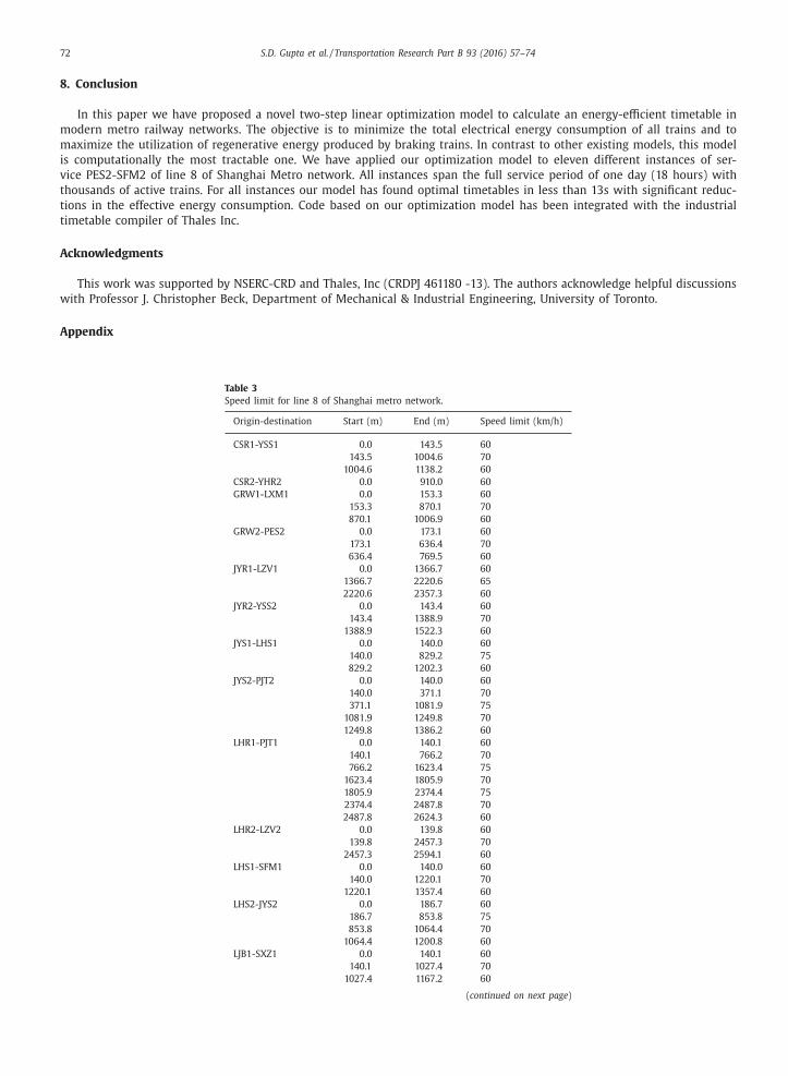
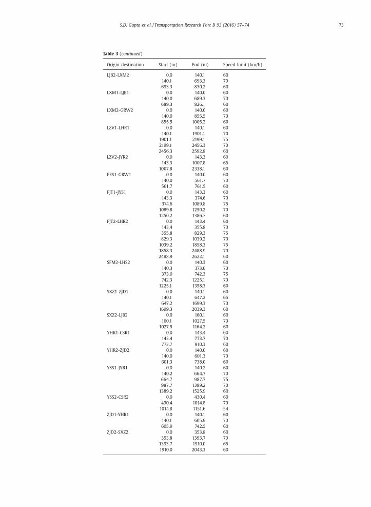
The data on speed limit is described by Table 3 in Appendix . The speed limit data are based on grade and curvature
of the tracks, and operational constraints present in the system. For the railway network, the tracks have piece-wise speed
limits for trains, i.e., each track (except CSR2-YHR2) is divided into multiple segments, where each segment has a constant
speed limit. The track CSR2-YHR2 has only one segment (itself) with a speed limit of 60 km/h. Table 3 is provided to us by
Thales Canada Inc.
The numerical study was executed on a Intel Core i7-46400 CPU with 8 GB RAM running Windows 8.1 Pro- operating
system. For modelling the problem, we have used JuMP - an open source algebraic modelling language embedded in pro-
gramming language Julia ( Lubin and Dunning, 2015 ). Within our JuMP code we have called academic version of Gurobi
Optimizer 6.0 as the solver. We have implemented an interior point algorithm because of the underlying sparsity in the
data structure. As mentioned before, a measure of the quality of affine fittings using least-squares approach is given by the
coefficient of determination , which can vary between 0 to 1, with 0 being the worst and 1 being the best ( Mendenhall et al.,
2009 , page 518). In our numerical study, the average coefficient of determination of the affine fittings for energy versus
trip times over all different trips and all trains is found to be 0.9483 with a standard deviation of 0.05, which justifies our
approach.
The duration of the timetables is eighteen hours which is the full service period of the railway network. We have consid-
ered eleven different instances with varying average headway times and number of trains. The number of trains increases
as the average headway time decreases, where the relation between them can be determined from Eq. 7 . The results of the
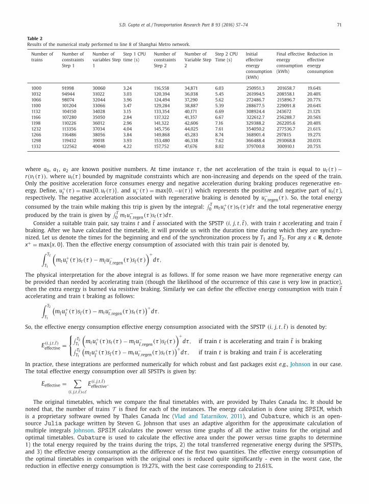
numerical study are shown in Table 2 .
We can see that, in all of the cases our model has found the optimal timetables very quickly, the largest runtime being
12.58s. To the best of our knowledge, this model is the only one to calculate energy-efficient railway timetable spanning an
entire day, the next largest being 6 hours only ( Das Gupta et al., 2015 ) with a much larger computation time for smaller
sized problems. After we get the final timetable, we calculate the total effective energy consumption by all trains involved
in SPSTPs and compare it with the original timetables. The effective energy consumption of a train during a trip is defined
as the difference between the total energy required to make a trip and the amount of energy that is being supplied by
a braking train during synchronization process. So, the effective energy consumption is the energy that will be consumed
from the electrical substations.
Now we briefly point out how the total energy consumption is calculated theoretically. Consider the trip of any train
t of mass m t from one platform to the next one. Assume the trip time to make the trip is T . At time instance τ , the
acceleration, speed, position, and resistive acceleration is denoted by u t ( τ ), v t ( τ ), s t ( τ ) and −r ( v t (τ ) ) , respectively. The
resistive acceleration is given by the Davis formula ( Davis, 1926 )
r ( v t (τ ) ) = a 0 + a 1 v t (τ ) + a 2 v 2 t (τ ) ,
S.D. Gupta et al. / Transportation Research Part B 93 (2016) 57–74 71
Table 2
Results of the numerical study performed to line 8 of Shanghai Metro network.
Number of
trains
Number of
constraints
Step 1
Number of
variables Step
1
Step 1 CPU
time (s)
Number of
constraints
Step 2
Number of
Variable Step
2
Step 2 CPU
Time (s)
Initial
effective
energy
consumption
(kWh)
Final effective
energy
consumption
(kWh)
Reduction in
effective
energy
consumption
10 0 0 91998 30060 3 .24 116,558 34,871 6 .03 250951 .3 201658 .7 19 .64%
1032 94944 31022 3 .03 120,394 36,038 5 .45 261994 .5 208558 .1 20 .40%
1066 98074 32044 3 .96 124,494 37,290 5 .62 272486 .7 215896 .7 20 .77%
1100 101204 33066 3 .47 129,284 38,887 5 .39 288677 .5 229091 .8 20 .64%
1132 104150 34028 3 .15 133,354 40,171 6 .69 308924 .4 243672 21 .12%
1166 107280 35050 2 .84 137,322 41,357 6 .67 322612 .7 256288 .7 20 .56%
1198 110226 36012 2 .96 141,322 42,606 7 .16 329388 .2 262205 .6 20 .40%
1232 113356 37034 4 .04 145,756 44,025 7 .61 354050 .2 277536 .7 21 .61%
1266 116486 38056 3 .84 14 9,86 8 45,283 8 .74 368901 .4 297815 19 .27%
1298 119432 39018 3 .93 153,480 46,338 7 .62 366488 .4 293068 .8 20 .03%
1332 122562 40040 4 .22 157,752 47,676 8 .02 379700 .8 300910 .1 20 .75%
where a 0 , a 1 , a 2 are known positive numbers. At time instance τ , the net acceleration of the train is equal to u t (τ ) −r ( v t (τ ) ) , where u t ( τ ) bounded by magnitude constraints which are non-increasing and depends on the speed of the train.
Only the positive acceleration force consumes energy and negative acceleration during braking produces regenerative en-
ergy. Define, u + t (τ ) = max { 0 , u t (τ ) } , and u −t (τ ) = max { 0 , −u (τ ) } which represents the positive and negative part of u t ( τ ),
respectively. The negative acceleration associated with regenerative braking is denoted by u −t, regen (τ ) . So, the total energy
consumed by the train while making this trip is given by the integral: ∫ T
0 m t u + t (τ ) s t (τ ) dτ and the total regenerative energy
produced by the train is given by ∫ T
0 m t u −t, regen (τ ) s t (τ ) dτ.
Consider a suitable train pair, say trains t and
˜ t associated with the SPSTP (i, j, t, t ) , with train t accelerating and train t
braking. After we have calculated the timetable, it will provide us with the duration time during which they are synchro-
nized. Let us denote the times for the beginning and end of the synchronization process by T 1 and T 2 . For any x ∈ R , denote
x + = max { x, 0 } . Then the effective energy consumption of associated with this train pair is denoted by, ∫ T 2
T 1
(m t u
+ t (τ ) s t (τ ) − m ˜ t u
−˜ t , regen
(τ ) s ˜ t (τ ) )+
dτ,
The physical interpretation for the above integral is as follows. If for some reason we have more regenerative energy can
be provided than needed by accelerating train (though the likelihood of the occurrence of this case is very low in practice),
then the extra energy is burned via resistive braking. Similarly we can define the effective ener gy consum ption with train t
accelerating and train t braking as follows: ∫ T 2
T 1
(m ˜ t u
+ ˜ t (τ ) s ˜ t (τ ) − m t u
−t, regen (τ ) s t (τ )
)+ dτ.
So, the effective energy consumption effective energy consumption associated with the SPSTP (i, j, t, t ) is denoted by:
E (i, j,t, t ) effective
=
{ ∫ T 2 T 1
(m t u
+ t (τ ) s t (τ ) − m ˜ t u
−˜ t , regen
(τ ) s ˜ t (τ ) )+
dτ, if train t is accelerating and train
˜ t is braking ∫ T 2 T 1
(m ˜ t u
+ ˜ t (τ ) s ˜ t (τ ) − m t u
−t, regen (τ ) s t (τ )
)+ dτ, if train t is braking and train
˜ t is accelerating
In practice, these integrations are performed numerically for which robust and fast packages exist e.g. , Johnson in our case.
The total effective energy consumption over all SPSTPs is given by:
E effective =
∑
(i, j,t, t ) ∈E E (i, j,t, t )
effective .
The original timetables, which we compare the final timetables with, are provided by Thales Canada Inc. It should be
noted that, the number of trains T is fixed for each of the instances. The energy calculation is done using SPSIM , which
is a proprietary software owned by Thales Canada Inc ( Vlad and Tatarnikov, 2011 ), and Cubature , which is an open-
source Julia package written by Steven G. Johnson that uses an adaptive algorithm for the approximate calculation of
multiple integrals Johnson . SPSIM calculates the power versus time graphs of all the active trains for the original and
optimal timetables. Cubature is used to calculate the effective area under the power versus time graphs to determine
1) the total energy required by the trains during the trips, 2) the total transferred regenerative energy during the SPSTPs,
and 3) the effective energy consumption as the difference of the first two quantities. The effective energy consumption of
the optimal timetables in comparison with the original ones is reduced quite significantly - even in the worst case, the
reduction in effective energy consumption is 19.27%, with the best case corresponding to 21.61%.
72 S.D. Gupta et al. / Transportation Research Part B 93 (2016) 57–74
8. Conclusion
In this paper we have proposed a novel two-step linear optimization model to calculate an energy-efficient timetable in
modern metro railway networks. The objective is to minimize the total electrical energy consumption of all trains and to
maximize the utilization of regenerative energy produced by braking trains. In contrast to other existing models, this model
is computationally the most tractable one. We have applied our optimization model to eleven different instances of ser-
vice PES2-SFM2 of line 8 of Shanghai Metro network. All instances span the full service period of one day (18 hours) with
thousands of active trains. For all instances our model has found optimal timetables in less than 13s with significant reduc-
tions in the effective energy consumption. Code based on our optimization model has been integrated with the industrial
timetable compiler of Thales Inc.
Acknowledgments
This work was supported by NSERC-CRD and Thales, Inc (CRDPJ 461180 -13). The authors acknowledge helpful discussions
with Professor J. Christopher Beck, Department of Mechanical & Industrial Engineering, University of Toronto.
Appendix
Table 3
Speed limit for line 8 of Shanghai metro network.
Origin-destination Start (m) End (m) Speed limit (km/h)
CSR1-YSS1 0 .0 143 .5 60
143 .5 1004 .6 70
1004 .6 1138 .2 60
CSR2-YHR2 0 .0 910 .0 60
GRW1-LXM1 0 .0 153 .3 60
153 .3 870 .1 70
870 .1 1006 .9 60
GRW2-PES2 0 .0 173 .1 60
173 .1 636 .4 70
636 .4 769 .5 60
JYR1-LZV1 0 .0 1366 .7 60
1366 .7 2220 .6 65
2220 .6 2357 .3 60
JYR2-YSS2 0 .0 143 .4 60
143 .4 1388 .9 70
1388 .9 1522 .3 60
JYS1-LHS1 0 .0 140 .0 60
140 .0 829 .2 75
829 .2 1202 .3 60
JYS2-PJT2 0 .0 140 .0 60
140 .0 371 .1 70
371 .1 1081 .9 75
1081 .9 1249 .8 70
1249 .8 1386 .2 60
LHR1-PJT1 0 .0 140 .1 60
140 .1 766 .2 70
766 .2 1623 .4 75
1623 .4 1805 .9 70
1805 .9 2374 .4 75
2374 .4 2487 .8 70
2487 .8 2624 .3 60
LHR2-LZV2 0 .0 139 .8 60
139 .8 2457 .3 70
2457 .3 2594 .1 60
LHS1-SFM1 0 .0 140 .0 60
140 .0 1220 .1 70
1220 .1 1357 .4 60
LHS2-JYS2 0 .0 186 .7 60
186 .7 853 .8 75
853 .8 1064 .4 70
1064 .4 1200 .8 60
LJB1-SXZ1 0 .0 140 .1 60
140 .1 1027 .4 70
1027 .4 1167 .2 60
( continued on next page )
S.D. Gupta et al. / Transportation Research Part B 93 (2016) 57–74 73
Table 3 ( continued )
Origin-destination Start (m) End (m) Speed limit (km/h)
LJB2-LXM2 0 .0 140 .1 60
140 .1 693 .3 70
693 .3 830 .2 60
LXM1-LJB1 0 .0 140 .0 60
140 .0 689 .3 70
689 .3 826 .1 60
LXM2-GRW2 0 .0 140 .0 60
140 .0 855 .5 70
855 .5 1005 .2 60
LZV1-LHR1 0 .0 140 .1 60
140 .1 1901 .1 70
1901 .1 2199 .1 75
2199 .1 2456 .3 70
2456 .3 2592 .8 60
LZV2-JYR2 0 .0 143 .3 60
143 .3 1007 .8 65
1007 .8 2338 .1 60
PES1-GRW1 0 .0 140 .0 60
140 .0 561 .7 70
561 .7 761 .5 60
PJT1-JYS1 0 .0 143 .3 60
143 .3 374 .6 70
374 .6 1089 .8 75
1089 .8 1250 .2 70
1250 .2 1386 .7 60
PJT2-LHR2 0 .0 143 .4 60
143 .4 355 .8 70
355 .8 829 .3 75
829 .3 1039 .2 70
1039 .2 1858 .3 75
1858 .3 2488 .9 70
2488 .9 2622 .1 60
SFM2-LHS2 0 .0 140 .3 60
140 .3 373 .0 70
373 .0 742 .3 75
742 .3 1225 .1 70
1225 .1 1358 .3 60
SXZ1-ZJD1 0 .0 140 .1 60
140 .1 647 .2 65
647 .2 1699 .3 70
1699 .3 2039 .3 60
SXZ2-LJB2 0 .0 160 .1 60
160 .1 1027 .5 70
1027 .5 1164 .2 60
YHR1-CSR1 0 .0 143 .4 60
143 .4 773 .7 70
773 .7 910 .3 60
YHR2-ZJD2 0 .0 140 .0 60
140 .0 601 .3 70
601 .3 738 .0 60
YSS1-JYR1 0 .0 140 .2 60
140 .2 664 .7 70
664 .7 987 .7 75
987 .7 1389 .2 70
1389 .2 1525 .9 60
YSS2-CSR2 0 .0 430 .4 60
430 .4 1014 .8 70
1014 .8 1151 .6 54
ZJD1-YHR1 0 .0 140 .1 60
140 .1 605 .9 70
605 .9 742 .5 60
ZJD2-SXZ2 0 .0 353 .8 60
353 .8 1393 .7 70
1393 .7 1910 .0 65
1910 .0 2043 .3 60
74 S.D. Gupta et al. / Transportation Research Part B 93 (2016) 57–74
References
Albrecht, A. , Howlett, P. , Pudney, P. , Vu, X. , Zhou, P. , 2015. The key principles of optimal train control - part 1: formulation of the model, strategies of
optimal type, evolutionary lines, location of optimal switching points. Transp. Res. Part B . Avinash Balakrishnan, K.S. (Ed.)2014. In: Nanostructured Ceramic Oxides for Supercapacitor Applications. CRC Press.
Bashash, S. , Moura, S.J. , Forman, J.C. , Fathy, H.K. , 2011. Plug-in hybrid electric vehicle charge pattern optimization for energy cost and battery longevity. J.
Power Sources 196 (1), 541–549 . Boyd, S. , Vandenberghe, L. , 2009. Convex Optimization. Cambridge university press .
Calafiore, G. , El Ghaoui, L. , 2014. Optimization Models. Cambridge University Press . Ciccarelli, F. , Del Pizzo, A. , Iannuzzi, D. , 2014. Improvement of energy efficiency in light railway vehicles based on power management control of wayside
lithium-ion capacitor storage. IEEE Trans. Power Electr. 29 (1), 275–286 . Das Gupta, S. , Pavel, L. , Kevin Tobin, J. , 2015. An optimization model to utilize regenerative braking energy in a railway network. In: American Control
Conference (ACC) .
Davis, W.J. , 1926. The Tractive Resistance of Electric Locomotives and Cars, vol. 29. General Electric Review . Droste-Franke, B. , Paal, B. , Rehtanz, C. , Sauer, D.U. , Schneider, J.-P. , Schreurs, M. , Ziesemer, T. , 2012. Balancing Renewable Electricity: Energy Storage, Demand
Side Management, and Network Extension from an Interdisciplinary Perspective, vol. 40. Springer Science & Business Media . González-Gil, A. , Palacin, R. , Batty, P. , 2013. Sustainable urban rail systems: Strategies and technologies for optimal management of regenerative braking
energy. Ener. Conversion Manage. 75, 374–388 . Group, S. S. M., 2015. Description of line 8, shanghai metro.
Harrod, S.S. , 2012. A tutorial on fundamental model structures for railway timetable optimization. Surv. Oper. Res. Manage. Sci. 17 (2), 85–96 .
Howlett, P. , 20 0 0. The optimal control of a train. Ann. Oper. Res. 98 (1–4), 65–87 . Howlett, P.G. , Pudney, P.J. , 1995. Energy-Efficient Train Control. Springer Science & Business Media .
Howlett, P.G. , Pudney, P.J. , Vu, X. , 2009. Local energy minimization in optimal train control. Automatica 45 (11), 2692–2698 . Jiaxin, C. , Howlett, P. , 1993. A note on the calculation of optimal strategies for the minimization of fuel consumption in the control of trains. IEEE Trans.
Autom. Control 38 (11), 1730–1734 . Johnson, S. G.,. The cubature module for julia. [Online]. Available: https://github.com/stevengj/Cubature.jl .
Kapadia, A.S. , Chan, W. , Moyé, L.A. , 2005. Mathematical Statistics with Applications. CRC Press . Khmelnitsky, E. , 20 0 0. On an optimal control problem of train operation. IEEE Trans. Autom. Control 45 (7), 1257–1266 .
Le, Z., Li, K., Ye, J., Xu, X., 2014. Optimizing the train timetable for a subway system. Proceedings of the Institution of Mechanical Engineers, Part F: Journal
of Rail and Rapid Transit doi: 10.1177/0954409714524377 . Li, X. , Lo, H.K. , 2014a. An energy-efficient scheduling and speed control approach for metro rail operations. Transp. Res. Part B 64, 73–89 .
Li, X. , Lo, H.K. , 2014b. Energy minimization in dynamic train scheduling and control for metro rail operations. Transp. Res. Part B 70, 269–284 . Liebchen, C. , 2007. Periodic timetable optimization in public transport. Springer .
Liu, R.R. , Golovitcher, I.M. , 2003. Energy-efficient operation of rail vehicles. Transp. Res. Part A 37 (10), 917–932 . Lubin, M., Dunning, I., 2015. Computing in operations research using julia. INFORMS J. Comput. 27 (2), 238–248. doi: 10.1287/ijoc.2014.0623 .
Mahajan, S. , 2010. Street-Fighting Mathematics. MIT Press Cambridge .
Mendenhall, W. , Beaver, R. , Beaver, B. , 2009. Introduction to probability and statistics. Cengage Learning . Milroy, I.P. , 1980. Aspects of Automatic Train Control. Ph.D. thesis Loughborough University of Technology .
Mura, R. , Utkin, V. , Onori, S. , 2013. Recasting the hev energy management problem into an infinite-time optimization problem including stability. In:Proceedings of IEEE 52nd Annual Conference on Decision and Control (CDC), pp. 6 837–6 842 .
Nuesch, T. , Ott, T. , Ebbesen, S. , Guzzella, L. , 2012. Cost and fuel-optimal selection of hev topologies using particle swarm optimization and dynamic pro-gramming. In: Proceedings of American Control Conference (ACC), pp. 1302–1307 .
Patil, R. , Kelly, J.C. , Filipi, Z. , Fathy, H. , 2012. A framework for the integrated optimization of charging and power management in plug-in hybrid electric
vehicles. In: Proceedings of American Control Conference (ACC), pp. 1327–1334 . Peeters, L. , 2003. Cyclic Railway Timetable Optimization. Ph.D. thesis Erasmus University Rotterdam .
Peña-Alcaraz, M. , Fernández, A. , Cucala, A.P. , Ramos, A. , Pecharromán, R.R. , 2012a. Optimal underground timetable design based on power flow for maxi-mizing the use of regenerative-braking energy. Proceedings of the Institution of Mechanical Engineers, Part F: Journal of Rail and Rapid Transit 226 (4),
397–408 . Peña-Alcaraz, M. , Webster, M. , Ramos, A. , 2012b. An approximate dynamic programming approach for designing train timetables. ESD Working Paper Series .
Saber, A.Y. , Venayagamoorthy, G.K. , 2010. Intelligent unit commitment with vehicle-to-grid: A cost-emission optimization. J. Power Sources 195 (3), 898–911 .
Schrijver, A. , 1998. Theory of Linear and Integer Programming. John Wiley & Sons . Vlad, E.P. , Tatarnikov, V. , 2011. R&M&A&S of communication based train control systems applied to urban rail transportation way to improve city sustain-
ability. In: Proceedings of IEEE Reliability and Maintainability Symposium (RAMS), pp. 1–6 . Yang, X. , Li, X. , Gao, Z. , Wang, H. , Tang, T. , 2013. A cooperative scheduling model for timetable optimization in subway systems. IEEE Trans. Intell. Transp.
Syst. 14 (1), 438–447 .
Further reading
Bombardier Inc., 2010. Energstor wayside energy storage. [Online]. Available: http://www.bombardier.com/content/dam/Websites/bombardiercom/ supporting- documents/BT/Bombardier- Transportation- ECO4- EnerGstor- EN.pdf .
Lu, M. , Beguin, F. , Frackowiak, E. , 2013. Supercapacitors: Materials, Systems and Applications. John Wiley & Sons .