TRER O M A

DIA

Universita degli Studi di Roma TreDipartimento di Informatica e AutomazioneVia della Vasca Navale, 79 – 00146 Roma, Italy

Rolling stock rostering

optimization

under maintenance constraints

Giovanni Luca Giacco1,2, Andrea D’Ariano1, Dario Pacciarelli1

RT-DIA-195-2012 Giugno 2012

(1) Universita degli Studi Roma Tre,Via della Vasca Navale, 79

00146 Roma, Italy.

(2) Direzione Pianificazione Industriale, Trenitalia S.p.A.,Piazza della Croce Rossa, 1

00161 Roma, Italy.

This work is partially supported by the Italian Ministry of Research, project FIRB “Ad-vanced tracking system in intermodal freight transportation”, Grant number RBIP06BZW8.We thank Trenitalia managers for their suggestions and support with railway data collec-tion and analysis. A preliminary version of this work was published in Giacco et al. [15].

ABSTRACT

This paper presents a mixed-integer linear-programming formulation for integrating short-term maintenance planning in a network-wide railway rolling stock circulation problem.This is a key problem in railway rostering planning that requires to cover a given set ofservices and maintenance works with a minimum amount of rolling stock units. In ourformulation, a rostering solution is viewed as a minimal cost Hamiltonian cycle in a graphwith service pairings, empty runs and short-term maintenance tasks. We use a commer-cial MIP solver to compute efficient solutions in a short time. Experimental results onreal-world scenarios from Trenitalia show that this integrated approach can reduce sig-nificantly the number of trains and empty runs when compared with the current rollingstock circulation plan.

Keywords: Railway Planning, Rolling Stock Circulation, Maintenance, Mixed-IntegerLinear-Programming.

2

1 INTRODUCTION

Problem under study

A main challenge of railway undertakings is to reduce the overall cost of railway operationsby means of a more efficient use of available resources, as well as rolling stock, crews andmaintenance resources [17]. Rolling stock circulation and short-term maintenance plan-ning are significant cost components for a railway company, which are typically managedby solving a number of interrelated problems [19, 21, 22].

The current practice of rolling stock rostering is focused on implementing slight mod-ifications to the previous plan in presence of new requests. This is mainly due to thedifficulty faced by planners when developing network-wide solutions manually. The com-putation of a globally feasible solution is already a very complex task and the plannershave little concern of the gap between their solutions and the optimal solutions relatedto specific performance indicators. Research in this context is therefore worth to searchfor better quality solutions of practical interest.

Related literature

Most of the scientific work considers the management of train rostering, the balancing ofempty runs and the cycles of rolling stock maintenance separately, even if these are partsof the same problem. In view of several recent reviews on this subject [1, 2, 8, 16, 18],we limit our literature discussion to research that deals with analytical approaches closelyrelated to this work.

Erlebach et al. [13] discuss the NP-hardness of the train rostering problem, includingthe special cases in which empty movements are allowed and rolling stock maintenanceis required. They work under the assumption that all trains are identical. They alsosimplify the maintenance scheduling by replacing an unmaintained train by a maintainedone, once they are at the same station.

Eidenbenz et al. [14] study a so-called flexible train rostering problem in which twolevels of flexibility are considered: the departure time of each route is free, but not theduration, and a delay threshold is given for each route. However, maintenance operationsare not included in their approach and there is no computational evidence of the potentialgain achievable by introducing flexible operations.

Maroti and Kroon [20] develop a multi-commodity flow model for preventive mainte-nance routing. Their basic idea is to improve an existing practical solution by implement-ing a limited number of changes to a macroscopic rolling stock plan in which rolling stockunits move on lines between aggregate stations. The objective function is related to theminimization of shunting plan deviations. Alfieri et al. [3] propose a multi-commodityflow model for efficient rolling stock circulation on a single line of the Dutch railway net-work. Their objective is to minimize the distance run by train units of various types.Short-term maintenance requirements are not considered in their formulations.

Budai et al. [6] provide a mathematical formulation for the long-term planning of rail-way maintenance works. The objective is to minimize the time required for maintenance,expressed as a cost function. Heuristic algorithms compute nearly-optimal solutions bycombining maintenance activities on each track.

Caprara et al. [9] study the train timetabling problem from an infrastructure manager

3

point of view: the objective is to improve the use of infrastructure resources. Maintenanceoperations are modeled as fixed constraints. An integer linear programming formulation isproposed and solved by a Lagrangian heuristic. Tests on a Italian test bed with differenttrain types show that maintenance constraints may seriously affect the quality of theoverall timetabling process.

Recently, Borndorfer et al. [5] study the assignment of rolling stock to timetableservices. A hypergraph based integer programming formulation is proposed for a cyclicplanning horizon of one week. In Cadarso and Marın [7], a more general rolling stockand train routing problem is addressed. The rolling stock subtask is to assign material tosatisfy the timetable of a railway network, while the train routing subtask is to determinethe best sequence for each material. Since the combined problem is not solvable bystandard MIP solvers, they propose a new heuristic based on Benders decomposition. Theobjective function of the overall approach is to minimize a cost-based function related tocommercial train services, empty movements, shunting and passengers in excess. Boththe latter analytical approaches do not model short-term maintenance operations and donot evaluate their cost impact.

Paper contribution

This work addresses jointly the daily rolling stock and maintenance aspects of the rosteringproblem. We present a new decision support system based on a mixed-integer linear-programming formulation. The general goal is to cover all services of a given timetable,as well as maintenance operations, while minimizing the use of rolling stock units (i.e.,trains). Given the departure and arrival times of each scheduled train service, the rosteringproblem is composed by three main tasks: (a) assign rolling stock units to the services,(b) schedule the maintenance tasks, (c) limit the number of empty runs. An empty runis a route between two stations with no assigned service, which is necessary when a trainmust cover in sequence two services and the arrival station of the first service is differentfrom the departing station of the second.

The specific objectives of our research are to address the following questions: “Howcan railway company efficiently manage their rolling stock? Which is the maximal im-provement that can be achieved?”. In this work, we address these questions by performingan incremental assessment of key performance indicators related to tasks a–c.

Methodology employed

The rolling stock rostering problem is viewed as the problem of finding a minimal costHamiltonian cycle in a graph in which the nodes correspond to train services and thearcs correspond to scheduling decisions, short-term maintenance operations and emptyruns. The objective function is to minimize the rolling stock units to cover all services.Additional performance indicators are improved by changing constraints on the bounds ofsome variables. The constraints of the rostering problem require that the different typesof maintenance operations must be carried out for each train periodically. The variousmaintenance tasks can only be done at a limited number of workshops.

The computational results are obtained by implementing and solving the proposedmodel with a commercial MIP solver. We tested a number of practical instances basedon timetable examples from Trenitalia (the main Italian railway company) for year 2011.

4

We reconstructed the services scheduled in the practical timetables as a benchmark forperformance evaluation. The real-life solutions are compared with those obtained by oursolution method in terms of the number of rolling stock units, the empty runs needed torealize the given timetables, and the distance run by trains between consecutive mainte-nance operations.

Paper organization

The next sections define the integrated problem of train rostering and maintenancescheduling, describe the mathematical formulation of this problem, present computa-tional experiments on real-world scenarios, discuss the obtained results and provide adescription of further research directions.

2 PROBLEM DESCRIPTION

The rolling stock rostering (RSR) problem is to determine a circulation for given scheduledruns. The general goal is to minimize the cost of the rolling stock assignment. The problemhas typically numerous requirements and constraints to be satisfied, that may differ foreach railway company [4, 10].

This paper studies a RSR problem with rolling stock and maintenance constraints par-ticularly relevant for Trenitalia. The proposed approach considers a macroscopic modelingof the railway traffic flow. The network is composed by a number of tracks and stations.A train route is a path between two given stations, with a given travel time. A trainservice i is a route from a departure station di at departure time td

i to an arrival stationai at arrival time ta

i that must be covered by a specific train. A roster is a cycle spanningover several working days that covers all the services and the required maintenance tasks.We assume that the same timetable is repeated every day. In other words, we study acyclic timetable and do not include, e.g., its variability in case of high/low demand daysor the inclusion of acyclic services, like long distance services. However, cyclic rosterscan be adapted to deal also with additional acyclic services. With our cyclic assumption,finding a roster spanning over k days allows to cover all services in a day with k trains.

A maintenance workshop is where maintenance work is performed and can coincidewith a station or not. Each maintenance workshop is dedicated to specific types of main-tenance work, such as: interior or exterior cleaning, refuel (only for diesel units), regularinspection, repair (scheduled or not) and technical check-up. Each type of maintenancetask must be performed regularly, i.e., within a maximum time limit or a maximum num-ber of kilometers from the last task of the same type. Since performing the same task toofrequently would cause an unnecessary cost for the company, each type of maintenancetask should be performed in the proximity of its maximum limit. It is known from theliterature that maintenance tasks may impose severe constraints on the RSR problem andtheir effect on the line capacity may be difficult to analyze [9].

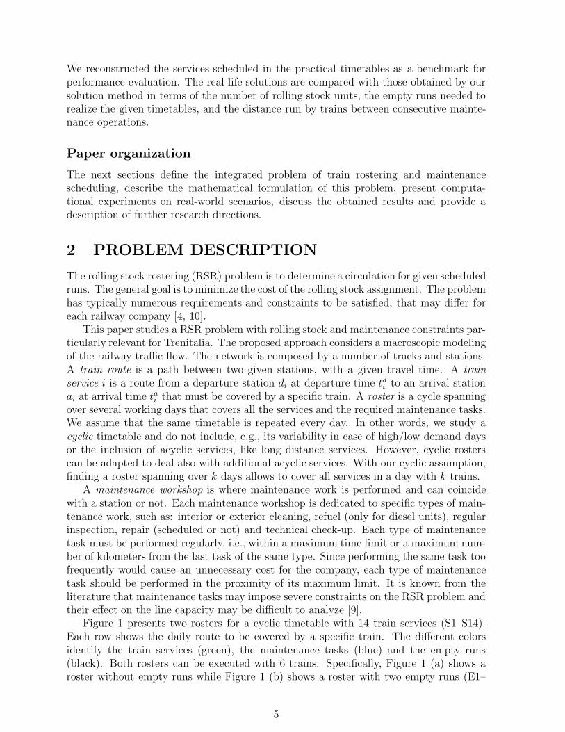
Figure 1 presents two rosters for a cyclic timetable with 14 train services (S1–S14).Each row shows the daily route to be covered by a specific train. The different colorsidentify the train services (green), the maintenance tasks (blue) and the empty runs(black). Both rosters can be executed with 6 trains. Specifically, Figure 1 (a) shows aroster without empty runs while Figure 1 (b) shows a roster with two empty runs (E1–

5

E2). The two schedules also differ in the number of maintenance tasks (3 in the first caseand 2 in the second one).

In Figure 1 (b), the two empty runs are added for moving the train correspondingto services S9 and S10 from Salerno to Napoli and from Napoli to Salerno. In thisway, the maintenance task M2’ can be performed at a maintenance workshop in Napoli.The maintenance tasks M2 and M3 are thus replaced by the maintenance task M2’.Specifically, the differences between the two rosters are the following:

• M1 and M1’ have approximately the same duration (around 12 hours), they areboth performed at a maintenance workshop in Rome, and their schedules are justshifted of a few minutes;

• M2 and M3 are both performed at a maintenance workshop in Rome and require(in total) around 19 hours, while M2’ is performed in Napoli and requires around16 hours. So, there is a gain of around 3 maintenance hours plus one less visit to amaintenance workshop for the roster of Figure 1 (b) compared to the one of Figure1 (a).

The comparison between the two rosters of Figure 1 shows how it is possible to reducethe number of maintenance tasks by using empty runs. From the one hand, the main-tenance costs are potentially reduced since less maintenance operations are performed inthe schedule of Figure 1 (b) compared to the one of Figure 1 (a). On the other hand, thecost of empty runs is increased since two empty runs are added in the schedule of Figure1 (b).

The specific problem addressed in this paper consists of finding a shortest roster,i.e., a sequence of all services spanning over the minimum number of days, such that allrequired maintenance tasks are inserted in the roster. Empty runs can be added to theroster in order to connect train services and/or to visit maintenance workshops. Althoughempty runs cause a relevant cost (e.g. related to additional energy consumption, rollingstock and crew resources) for the company and increase the traffic in the network, theirinclusion may help to reduce the maintenance cost and the roster length. For the abovereasons, optimizing the scheduling of maintenance tasks, trains services and empty runsis an important contribution to reduce the overall company costs. However, we noticethat the overall cost of a solution is difficult to evaluate. In fact, besides its monetaryvalue, a solution is also characterized by the utilization of track capacity, maintenanceworkshops and other resources. Therefore, in this paper we analyze separately the maincomponents affecting the cost of a solution, i.e., the number of rolling stock units, theamount of maintenance tasks and the number of empty runs.

The input data of the problem include: the rolling stock asset; the timetables and thescheduled train services; the maximum number allowed of empty runs; the railway in-frastructure; the location and characteristics of maintenance workshops; the maintenancetasks to perform and time windows of [minimum, maximum] number of kilometers foreach maintenance task.

Clearly, allowing a larger number of empty runs or larger time windows for the main-tenance tasks corresponds to leaving greater flexibility to minimize the number of rollingstock units. The effects of flexibility on the efficient management of assets such as trains,infrastructure elements and staff have been assessed, e.g., by [9, 11, 12].

In the computational experiments presented in this paper, we investigate the interac-tion between the minimum number of trains needed to perform all services and different

6

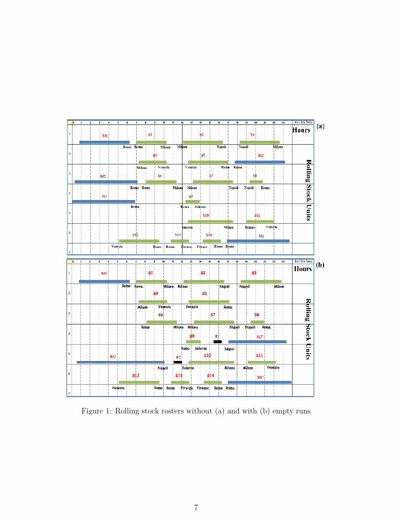
Figure 1: Rolling stock rosters without (a) and with (b) empty runs

7

values for the maximum number of empty runs, and for the time windows of the distancecovered between consecutive maintenance operations of the same type. We also evaluatethe efficiency of the optimization-based solutions compared with the practical ones interms of these three performance indicators.

3 PROBLEM FORMULATION

In this section we introduce the problem notation and the formulation of the RSR problem.The notation is also listed in the Appendix of the paper.

The RSR problem is represented by a graph G = (V,A) in which the set of nodes Vcontains the n train services to be included in the roster, while each arc in A models afeasible sequencing of train services in a roster, plus the possible inclusions of empty runsand/or maintenance tasks.

There can be several types of arcs between two nodes i and j, and we denote by zthe type of arc (i, j, z) and by Z the set of arc types. If the arrival station ai of service iis equal to the departure station dj of service j, we add to A an arc of type z =waitingbetween i and j and, possibly, an arc of type z =maintenance for each type of maintenancetask m that can be executed in the proximity of station ai, i.e., such that the distancebetween ai and the closest maintenance workshop enabled to perform m is smaller thana pre-defined value.

If ai 6= dj , we can add to A an arc (i, j, z) of type z =empty run plus an arc for eachmaintenance task that can be processed in a maintenance workshop close the route fromai to dj.

Each arc (i, j, z) has a cost cijz equal to the time lag (i.e., the number of days) re-quired to process j after the completion of i, which is zero if i and j can be performedconsecutively in the same day. When z =maintenance or z =empty run, other valuesassociated to arc (i, j, z) are: the distance K1

ijz from ai to the maintenance workshop, thedistance K2

ijz from the maintenance workshop to dj, and the distance K3ijz from ai to dj

(only in case of empty run. Figure 2 shows a simple example with two services (fromRome to Naples and from Udine to Rome), a maintenance workshop and two empty runpossibilities: including (see the dotted black arcs) or not including a maintenance work(see the solid black arc) when moving from Naples to Udine with an empty run.

Figure 2: Example of empty run and maintenance tasks

In order to compute cijz, we must preliminarily compute the time lag between the twoservices i and j, which depends on the arc type:

• If di = aj and z =waiting, the time lag must only take into account the minimumslack time between the two services;

8

• if di = aj and z =maintenance, the time lag must also take into account the main-tenance time window needed to execute maintenance works for the rolling stockinvolved, plus the travel time to reach the maintenance workshop and come back;

• if di 6= aj and z =empty run, the time lag must take into account the time needed toreach aj plus, possibly, the slack time and the maintenance time needed to performthe prescribed maintenance tasks. For the example in Figure 2, the cost of the solidarc is one, since the second service can start only the day after the arrival in Naples.The cost of the dotted arc can be even two or more, depending on the time neededto perform the maintenance task.

Note that the feasibility of a Hamiltonian cycle passing through arc (i, j, z) also dependson the maintenance status of the rolling stock at node i. In fact, the distance elapsedbetween i and j plus the rolling stock status at i must be compatible with the maintenancewindows for all maintenance tasks. To compute the rolling stock maintenance status, foreach arc (i, j, z) and for each maintenance type m, we introduce a real variable gm

ijz thatcounts the distance covered by each train since the last maintenance task of type m wasperformed. A solution is feasible if gm

ijz is bounded between a minimum βm and a maximumγm on the distance (in kilometers) run by a train between consecutive executions of taskm, i.e., βm ≥ gm

ijz ≥ γm.In conclusions, the rostering problem can be viewed as the problem of finding a mini-

mum cost Hamiltonian cycle in G with additional constraints related to the implementa-tion of maintenance tasks.

Illustrative example

Figure 3 shows a small graph to illustrate the problem formulation. For each train service,there is a (red) node, with labels indicating departure and arrival stations plus the asso-ciated times. The solid black arcs (set A1) indicate the empty runs without maintenance,the dotted black arcs (set A2) the empty runs with maintenance tasks, the blue arcs (setA3) the maintenance tasks without empty runs, the green arcs (set A4) the service pair-ings. The numeric labels show arc costs, while non-numeric labels indicate maintenancetypes (M1, M2 and their combination M1+M2). For simplicity, the maintenance costsare not shown in the graph.

The three services (Napoli-Udine, Udine-Roma and Roma-Napoli) of Figure 3 requirea number of trains, maintenance works and empty runs. A solution is a Hamiltonian pathwith maintenance operations constraints. In the solution the empty runs (black arcs) areoptional.

9

Figure 3: A graph formulation for three train services

Variables

The proposed formulation considers three types of variables: X is a set of binary variablessuch that xijz ∈ X is equal to 1 if arc (i, j, z) belongs to the Hamiltonian cycle and zerootherwise, Y is a set of integer variables that are used for sub-tour elimination, G is aset of real variables that are used to count the distance run by each train between twoconsecutive executions the same maintenance task. If xijz = 1 then the distance betweentwo consecutive executions of task m must be always between a lower bound βm and anupper bound γm. In a solution, the variables in Y and G can be derived from the variablesin X.

Objective function

The objective function is the minimization of the number of days included in the rosteror, equivalently, the number of trains required to perform all services in a day:

∑

(i,j,z)∈A

cijzxijz

where cijz is the cost of arc (i, j, z) ∈ A.

Path constraints

The first set of constraints is:

(I)

∑i∈V

∑z:(i,h,z)∈A

xihz = 1∑

j∈V

∑z:(h,j,z)∈A

xhjz = 1∀h ∈ V

Equation (I) prescribes that there must be exactly one predecessor and one successorfor each node h ∈ V .

10

Sub-tour elimination constraints

This set of constraints is introduced for modeling the roster as an Hamiltonian cycle. Thebasic idea to avoid sub-tours is the use of node labels that count the order of nodes in thesolution, beginning from a first node n0 = 1 randomly chosen. Along the path, the labelof each visited node is increased by one unit compared with the previous node (except forn0). Hence, the value of labels is from 1 to n and two nodes cannot have the same label.

In the problem formulation, an integer variable ykj ∈ Y is associated to each pair ofnodes k, j ∈ V , with k 6= j, such that:

(II)∑i∈V

yji =∑

k∈Vykj + 1 ∀j ∈ V \ {n0}

(III) 0 ≤ yij ≤ n∑

(ijz)∈Axijz ∀yij ∈ Y

(IV)∑i∈V

yn0i = 1

Equation (II) constrains the sum of the arcs entering each node, but n0, to be equal tothe sum of the arcs leaving the same node plus 1. Equation (III) constrains the arc labelvalues to be greater than 0 if and only if a variable xijz ∈ X of type z exists between nodesi and j with value greater than 0. With these equations, there is just one arc leaving andone arc entering each node with yij > 0. If two services i and j are executed consecutively(i.e., if there is a variable xijz = 1), the label of j is equal to the one of i plus 1. Equation(IV) forces all arcs outgoing node n0 to be numbered 1.

Figure 4: Example of sub-tour situation

Figure 4 shows an example situation with two sub-tours in the graph. Only arcs withvariables x = 1 are shown in the figure. This solution violates Equation II for sub-tour4,5,6. In fact, y45 = y64 + 1, y56 = y45 + 1, and y64 = y56 + 1 must hold, thus implyingy45 = y45 + 3, which is impossible.

11

Maintenance constraints

Maintenance tasks need to be performed within a given time window of maintenance.However, the intention is to prevent the execution of an excessive number of maintenancetasks. In general, the less are the maintenance tasks the more cost effective is the overallsolution.

The formulation of maintenance tasks requires the introduction of a new variable gmijz

for each maintenance task of type m and for each arc (i, j, z) ∈ A. This variable countsthe kilometers run by a train from the last maintenance task of type m, and it is set to 0when the maintenance task m is performed.

Let us introduce some further notation. Ki is the distance run by train service i, Am

[Am] is the set of service pairings, empty runs and maintenance tasks that include [do notinclude] maintenance task m. Am

I [AmI ] is the set of empty run arcs with maintenance

tasks that include [do not include] task m in a maintenance workshop at the beginning oftheir route, Am

II [AmII] is the set of empty run arcs with maintenance tasks that include [do

not include] task m in a maintenance workshop at the end of their route, AmIII [Am

III] isthe set of empty run arcs with maintenance tasks that include [do not include] task m ina maintenance workshop in the middle of their route. The maintenance constraints are:

∑l∈V

∑z∈Zj,l

gmjlz = Kj +

∑i∈V

∑z∈Zi,j :(i,j,z)∈Am

gmijz+

(V )∑

(i,j,z)∈AmIII

K2ijzxijz +

∑(i,j,z)∈Am

I

K3ijzxijz+ ∀j ∈ V,∀m

∑(j,l,z)∈Am

III

K1jlzxjlz +

∑(j,l,z)∈Am

I∪Am

II∪Am

III∪Am

II∪A1

K3jlzxjlz

(VI) gmijz ≤ γmxijz ∀(i, j, z) ∈ A,∀m

(VII) gmijz ≥ βmxijz ∀(i, j, z) ∈ A2 ∪ A3 : m ∈ Zi,j .

Equation (V) counts the distance covered by each train, including the empty runs, fromthe last execution of a maintenance task of type m to the end of service j. Note that, sincethere is exactly one arc outgoing node j such that xjlz = 1, the first term

∑l∈V

∑z∈Zj,l

gmjlz is

equal to the single variable gmjlz > 0 and must take into account the distance covered at

the end of service j. The following terms take into account the distance covered by thetrain related to service j: the distance Kj run by the train when performing service j,the cumulative distance covered by the train, including the empty runs, at the end of theservice i performed immediately before j if no maintenance task of type m is performedbetween i and j. The subsequent two terms of Equation (V) take into account the distancecovered during a possible empty run between i and j including a maintenance task of typem performed along the route from ai to dj or at station ai, respectively. The last twoterms of Equation (V) take into account the situation in which a maintenance task oftype m is performed between the end of service j and the start of service l. In this casethe quantity K1

jlz must be taken into account to ensure that the total distance coveredbefore the maintenance task is in the window (βm, γm). The last case arises when themaintenance is performed at station dj before the starting of service l. Note that, if a

12

maintenance task of type m is performed during an empty run, only the distance coveredafter the maintenance must be considered.

With reference to node j, Figure 5 shows the types of ingoing and outgoing arcs andthe corresponding distance to be covered. For the ingoing arcs to node j, each train coversgm

ijz in case of no maintenance of type m, K3ijz in case of empty run with maintenance of

type m at the beginning of its route, K2ijz in case of empty run with maintenance of type

m in the middle of its route, 0 otherwise. For the outgoing arcs from node j, each traincovers K3

jlz in case of empty run without maintenance tasks or with the maintenance taskof type m at the end of its route, K1

jlz in case of empty run with maintenance of type min the middle of its route, 0 otherwise.

Figure 5: Computation of the distance covered before and after node j

Equation (VI) constrains the distance to be covered after a task of type m to besmaller than the upper bound γm, while equation (VII) constrains the distance to becovered before a task of type m to be at least equal to the lower bound βm. The deadlineof each basic maintenance task is thus constrained, even if it is sometimes possible tocombine basic maintenance operations in multifunctional workshops.

Bound constraints on the empty runs

This type of constraints defines the maximum number of empty runs permitted in asolution:

(VIII)∑

(i,j,z)∈A1∪A2

xijz ≤ α

where the bound α is an input parameter related to the maximum number of emptyruns allowed in a solution.

4 COMPUTATIONAL EXPERIMENTS

This section presents a set of computational experiments on real-world cases from theTrenitalia timetable of year 2011. We consider practical rosters and solve the proposedmodel with CPLEX MIP solver 12.0.

13

Description of the instances

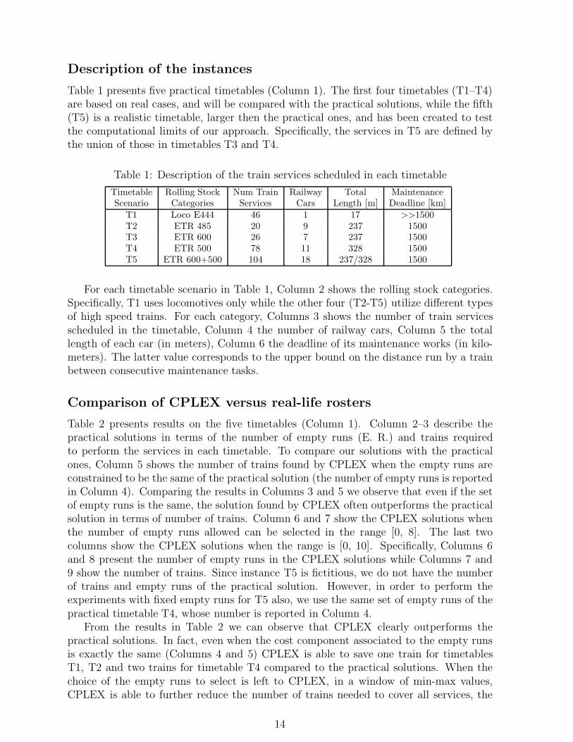
Table 1 presents five practical timetables (Column 1). The first four timetables (T1–T4)are based on real cases, and will be compared with the practical solutions, while the fifth(T5) is a realistic timetable, larger then the practical ones, and has been created to testthe computational limits of our approach. Specifically, the services in T5 are defined bythe union of those in timetables T3 and T4.

Table 1: Description of the train services scheduled in each timetable

Timetable Rolling Stock Num Train Railway Total MaintenanceScenario Categories Services Cars Length [m] Deadline [km]

T1 Loco E444 46 1 17 >>1500T2 ETR 485 20 9 237 1500T3 ETR 600 26 7 237 1500T4 ETR 500 78 11 328 1500T5 ETR 600+500 104 18 237/328 1500

For each timetable scenario in Table 1, Column 2 shows the rolling stock categories.Specifically, T1 uses locomotives only while the other four (T2-T5) utilize different typesof high speed trains. For each category, Columns 3 shows the number of train servicesscheduled in the timetable, Column 4 the number of railway cars, Column 5 the totallength of each car (in meters), Column 6 the deadline of its maintenance works (in kilo-meters). The latter value corresponds to the upper bound on the distance run by a trainbetween consecutive maintenance tasks.

Comparison of CPLEX versus real-life rosters

Table 2 presents results on the five timetables (Column 1). Column 2–3 describe thepractical solutions in terms of the number of empty runs (E. R.) and trains requiredto perform the services in each timetable. To compare our solutions with the practicalones, Column 5 shows the number of trains found by CPLEX when the empty runs areconstrained to be the same of the practical solution (the number of empty runs is reportedin Column 4). Comparing the results in Columns 3 and 5 we observe that even if the setof empty runs is the same, the solution found by CPLEX often outperforms the practicalsolution in terms of number of trains. Column 6 and 7 show the CPLEX solutions whenthe number of empty runs allowed can be selected in the range [0, 8]. The last twocolumns show the CPLEX solutions when the range is [0, 10]. Specifically, Columns 6and 8 present the number of empty runs in the CPLEX solutions while Columns 7 and9 show the number of trains. Since instance T5 is fictitious, we do not have the numberof trains and empty runs of the practical solution. However, in order to perform theexperiments with fixed empty runs for T5 also, we use the same set of empty runs of thepractical timetable T4, whose number is reported in Column 4.

From the results in Table 2 we can observe that CPLEX clearly outperforms thepractical solutions. In fact, even when the cost component associated to the empty runsis exactly the same (Columns 4 and 5) CPLEX is able to save one train for timetablesT1, T2 and two trains for timetable T4 compared to the practical solutions. When thechoice of the empty runs to select is left to CPLEX, in a window of min-max values,CPLEX is able to further reduce the number of trains needed to cover all services, the

14

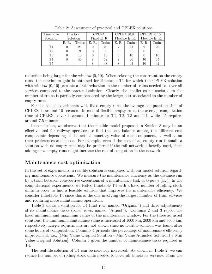
Table 2: Assessment of practical and CPLEX solutions

Timetable Practical CPLEX: CPLEX [0,8]: CPLEX [0,10]:Scenario Solution Fixed E. R. Flexible E. R. Flexible E. R.

E. R. Trains E. R. Trains E. R. Trains E. R. TrainsT1 0 26 0 25 7 21 9 20T2 0 9 0 8 0 8 0 8T3 0 10 0 10 0 10 0 10T4 8 40 8 38 8 36 10 35T5 - - 8 48 8 43 10 42

reduction being larger for the window [0, 10]. When relaxing the constraint on the emptyruns, the maximum gain is obtained for timetable T1 for which the CPLEX solutionwith window [0, 10] presents a 23% reduction in the number of trains needed to cover allservices compared to the practical solution. Clearly, the smaller cost associated to thenumber of trains is partially compensated by the larger cost associated to the number ofempty runs.

For the set of experiments with fixed empty runs, the average computation time ofCPLEX is around 10 seconds. In case of flexible empty runs, the average computationtime of CPLEX solver is around 1 minute for T1, T2, T3 and T4, while T5 requiresaround 7.5 minutes.

In conclusion, we observe that the flexible model proposed in Section 3 may be aneffective tool for railway operators to find the best balance among the different costcomponents depending of the actual monetary value of each component, as well as ontheir preferences and needs. For example, even if the cost of an empty run is small, asolution with no empty runs may be preferred if the rail network is heavily used, sinceadding new empty runs might increase the risk of congestion in the network.

Maintenance cost optimization

In this set of experiments, a real life solution is compared with our model solution regard-ing maintenance operations. We measure the maintenance efficiency as the distance runby a train between consecutive executions of a maintenance task of type m (βm). In thecomputational experiments, we tested timetable T4 with a fixed number of rolling stockunits in order to find a feasible solution that improves the maintenance efficiency. Weconsider timetable T4 since this is the one involving the largest number of train servicesand requiring more maintenance operations.

Table 3 shows a solution for T4 (first row, named “Original”) and three adjustmentsof its maintenance tasks (other rows, named “Adjust”). Columns 2 and 3 report thefixed minimum and maximum values of the maintenance window. For the three adjustedsolutions, the minimum maintenance value is increased of 1000 km, 2000 km and 3000 km,respectively. Larger adjustments are not shown since no feasible solution was found aftersome hours of computation. Columns 4 presents the percentage of maintenance efficiencyimprovement, i.e., [(Min Value Original Solution - Min Value Adjusted Solution) / MinValue Original Solution]. Column 5 gives the number of maintenance tasks required inT4.

The real-life solution of T4 can be seriously increased. As shown in Table 2, we canreduce the number of rolling stock units needed to cover all timetable services. From the

15

Table 3: Optimization of the maintenance efficiency

Instance Min Value [Km] Max Value [Km] Improvement [%] Maintenance tasksOriginal 5688 13040 - 6Adjust1 6688 13040 18 5Adjust2 7688 13040 35 5Adjust3 8688 13040 53 5

results of Table 3, there is also a considerable improvement of the maintenance efficiency(up to 53%) and a reduction of the required number of maintenance tasks. We believethat the monetary values of maintenance cost reduction can also be assessed by referringto the performance indicators in Table 3, in addition to limiting the number of emptyruns.

Flexible values for the empty runs

Figure 6 shows a third set of experiments in which we consider the empty runs as additionalvariables that can be selected in a range of min-max values. The experiments are based onthe five timetables and use different settings of the maximum number of empty runs. Weshow on y-axis the number of trains needed for the roster and on the x-axis the maximumnumber of empty runs.

Figure 6: Measuring the compromise between rolling stock units and empty runs

From the results of Figure 6, we have the following observations. For T2 and T3,increasing the empty runs has no effect on the rolling stock required to run all services,while for T1, T4 and T5 the rolling stock used is progressively reduced.

Considering T4, the practical solution (with 40 trains and 8 empty runs) can beimproved by two actions: reducing the number of trains and/or limiting the number ofempty runs. When comparing the practical solution versus the optimal solution of our

16

model, there is a trade-off between the two actions for the two cases with 9 and 10 emptyruns. For smaller values of empty runs, our model gives always better solutions than thepractical one for both performance indicators. In the solution with 8 empty runs, thenumber of trains can be reduced up to 10%.

5 CONCLUSIONS AND FURTHER RESEARCH

This paper presents a new approach for optimizing rolling stock rostering and short-termmaintenance planning. The mathematical problem is to find a minimal cost Hamiltoniancycle in a graph with service pairings, empty runs and maintenance tasks. Computationalexperiments are performed on a commercial MIP solver and show a thorough assessmentof timetables and rosters. The proposed approach is considerably effective in reducing thecompany costs compared to the practical solutions, both with and without consideringflexibility of rail operations. Specifically, we tried to answer the question: Is it possible toimprove the practical solutions firstly in terms of the number of trains needed to cover allservices, and then in terms of the number of empty runs and the maintenance efficiency?In fact, this is achieved by improving one by one these performance indicators.

Future research will be dedicated to the development of even more sophisticated formu-lations. We are studying how define objective functions directly related to the monetaryvalues of circulation, empty runs and maintenance, representing the preferences of therailway company. Another issue is the extension of our model to include detailed schedul-ing of maintenance operations in station areas. Open issues are related to balance the useof resources when routing trains in wide-networks and to the limit the workload for theoperators at maintenance workshops. Further research directions should also be focusedon developing methods for acyclic timetables and advanced algorithms for complex andlarge instances.

References

[1] Abril, M., F. Barber, L. Ingolotti, M.A. Salido, P. Tormos, Lova, A. (2008) Anassessment of railway capacity. Transportation Research Part E, Vol. 44(5), pp. 774–806

[2] Ahuja, R.K., Cunha, C.B., Sahin, G. (2005) Network Models in Railroad Plan-ning and Scheduling. TutORials in Operations Research, H.J. Greenberg, J.C. Smith(Eds.), pp. 54–101

[3] Alfieri, A., Groot, R., Kroon, L.G., Schrijver, A. (2006) Efficient circulation of railwayrolling stock. Transportation Science, Vol. 40(3), pp. 378–391

[4] Anderegg, L., Eidenbenz, S., Gantenbein, M., Stamm, C., Taylor, D.S., Weber, B.,Widmayer, P. (2003) Train Routing Algorithms: Concepts, Design Choices, andPractical Considerations. Proceedings of the Fifth Workshop on Algorithm Engineer-ing and Experiments (Proceedings in Applied Mathematics), R.E. Ladner (Ed.), pp.106–118

17

[5] Borndorfer, R., Reuther, M., Schlechte, T., Weider, S. (2011) A Hypergraph Modelfor Railway Vehicle Rotation Planning. Proceedings of the 11th Workshop on Al-gorithmic Approaches for Transportation Modelling, Optimization, and Systems, A.Caprara, S. Kontogiannis (Eds.), Saarbrucken, Germany

[6] Budai, G., Huisman, D., Dekker, R. (2006) Scheduling Preventive Railway Mainte-nance Activities. Journal of the Operational Research Society, Vol. 57(9), pp. 1035–1044

[7] Cadarso, L., Marın, A. (2011) Robust Rolling Stock and Routing Integration inRapid Transit Networks. Proceedings of the 4th International Seminar on RailwayOperations Modelling and Analysis, S. Ricci, I.A. Hansen, G. Longo, D. Pacciarelli,J. Rodriguez, E. Wendler (Eds.), Universita degli Studi “La Sapienza”, Italy

[8] Caprara, A., Kroon, L.G., Monaci, M., Peeters, M., Toth, P. (2006) Passenger Rail-way Optimization. Handbooks in Operations Research and Management Science, C.Barnhart, G. Laporte (Eds.), pp. 129–187

[9] Caprara, A., Monaci, M., Toth, P., Guida, P.L. (2006) A Lagrangian heuristic algo-rithm for a real-world train timetabling problem. Discrete Applied Mathematics, Vol.154(5), pp. 738–753

[10] Confessore, G., Liotta, G., Cicini, P., Rondinone, F., De Luca, P. (2009) A simulation-based approach for estimating the commercial capacity of railways. Proceedings ofthe 2009 Winter Simulation Conference, M.D. Rossetti, R.R. Hill, B. Johansson, A.Dunkin and R.G. Ingalls (Eds.), Austin, Texas, USA

[11] Corman, F., D’Ariano, A., Pacciarelli, D., Pranzo, M. (2010) Railway dynamic trafficmanagement in complex and densely used networks. In R.R. Negenborn, Z. Lukszo,H. Hellendoorn (Eds.), Intelligent Infrastructures, Intelligent Systems, Control andAutomation: Science and Engineering Vol. 42, pp. 377–404

[12] D’Ariano, A., Pacciarelli, D., Pranzo, M. (2008) Assessment of flexible timetables inreal-time traffic management of a railway bottleneck. Transportation Research, PartC, Vol. 16(2), pp. 232–245

[13] Erlebach, T., Gantenbein, M., Hurlimann, D., Neyer, G., Pagourtzis, A., Penna, P.,Schlude, K., Steinhofel, K., Taylor, D.S., Widmayer, P. (2001) On the Complexityof Train Assignment Problems. Lecture Notes in Computer Science, Vol. 2223, pp.390–402

[14] Eidenbenz, S., Pagourtzis, A., Widmayer, P. (2003) Flexible Train Rostering. LectureNotes in Computer Science, Vol. 2906, pp. 615–624

[15] G.L. Giacco, A. DAriano, D. Pacciarelli, Rolling stock rostering optimization undermaintenance constraints, Proceedings of the 2nd International Conference on Modelsand Technology for Intelligent Transportation Systems (MT-ITS 2011), F. Viti (Ed.),Leuven, Belgium

[16] Hansen, I.A., Pachl, J. (Eds.) (2008) Railway Timetable and Traffic: Analysis, Mod-elling and Simulation, Eurailpress, Hamburg, Germany

18

[17] Kontaxi, E., Ricci, S. (2010) Railway capacity analysis: Methodological frameworkand harmonization perspectives. Proceedings of the 12th World Conference on Trans-port Research (WCTR 2010), J. Viegas, R. Macario (Eds.), Lisbon, Portugal

[18] Lusby, R.M., Larsen, J., Ehrgott, M., Ryan, D. (2011) Railway track allocation:models and methods. OR Spectrum, Vol. 33(4), pp. 843–883

[19] Marinov, M., Viegas, J. (2011) A mesoscopic simulation modelling methodology foranalyzing and evaluating freight train operations in a rail network. Simulation Mod-elling Practice and Theory, Vol. 19(1), pp. 516–539

[20] Maroti, G., Kroon, L.G. (2005) Maintenance routing for train units: the transitionmodel. Transportation Science, Vol. 39(4), pp. 518–525

[21] Santos, R., Teixeira, P.F. (2011) Heuristic Analysis of the Effective Range of a TrackTamping Machine. Journal of Infrastructure Systems, IN PRESS

[22] Schlechte, T. (2011) Railway Track Allocation - Simulation and Optimization. Pro-ceedings of the 4th International Seminar on Railway Operations Modelling and Anal-ysis, S. Ricci, I.A. Hansen, G. Longo, D. Pacciarelli, J. Rodriguez, E. Wendler (Eds.),Universita degli Studi “La Sapienza”, Italy

APPENDIX: List of notations

This appendix lists the notation used in the paper.

• G = (V,A) is a graph with V nodes and A arcs

• V is the set of train services (i.e., the set of nodes)

• n is the cardinality of the set V

• di is the departure station of service i with departure time tdi

• ai is the arrival station of service i with arrival time tdi

• A1 is the set of empty run arcs without maintenance tasks (i.e., the set of solid blackarcs)

• A2 is the set of empty run arcs with maintenance tasks (i.e., the set of dotted blackarcs)

• A3 is the set of maintenance arcs without empty runs (i.e., the set of blue arcs)

• A4 is the set of service pairings (i.e., the set of green arcs)

• A is the set of all arcs: service pairings, empty runs and maintenance tasks (A =A1

⋃A2

⋃A3

⋃A4)

19

• Am (Am) is the set of service pairings, empty runs and maintenance tasks that (donot) include maintenance task m

• AmI (Am

I ) is the set of empty run arcs with maintenance tasks that (do not) includetask m in a maintenance workshop at the beginning of their route

• AmII (Am

II) is the set of empty run arcs with maintenance tasks that (do not) includetask m in a maintenance workshop at the end of their route

• AmIII (Am

III) is the set of empty run arcs with maintenance tasks that (do not) includetask m in a maintenance workshop in the middle of their route

• Z is the set of arc types

• (i, j, z) is an arc between start node i and end node j of type z ∈ Z

• cijz is the cost of arc (i, j, z)

• Ki are the kilometers of train service i

• K1ijz is the distance to be covered by a train (associated to arc (i, j, z)) from ai to a

maintenance workshop in case of empty run

• K2ijz is the distance to be covered by a train (associated to arc (i, j, z)) from a

maintenance workshop to dj in case of empty run

• K3ijz is the distance to be covered by a train (associated to arc (i, j, z)) from ai to

dj in case of empty run

• α is a bound related to the maximum number of empty runs allowed in a solution

• βm is a lower bound on the distance run by a train between consecutive executionsof task m

• γm is an upper bound on the distance run by a train between consecutive executionsof task m

• X is a set of binary variables

• Y is a set of integer variables

• G is a set of real variables

• gmijz ∈ G counts the kilometers run by a train from the last maintenance task of type

m

• xijz ∈ X is equal to 1 if arc (i, j, z) belongs to the Hamiltonian cycle and zerootherwise

• ykj ∈ Y is associated to each pair of nodes k, j ∈ V such that sub-tours can berecognized and eliminated

20