TRIP ASSIGNMENT

Trip Assignment is the procedure by which the planner/engineer predicts the paths the trips will take.

For example, if a trip goes from a suburb to downtown, the model predicts the specific streets or transit routes to be used.

Trip Assignment Procedures

1.Minimum-Path Techniques.

•Minimum-path techniques are based on the assumption that travelers want to use the minimum impedance route between two points. •The trip between zones are loaded onto the links making up the minimum path. This technique is sometimes referred to as “all-or-nothing” because all trips between a given origin and destination are loaded on the links comprising the minimum path and nothing is loaded on the other links.•After all possible interchanges are considered, the result is an estimate of the volume on each link in the network.•This method can cause some links to be assigned more travel volume than the link has capacity at the original assumed speed.

Example: Assign the vehicle trips shown in the O-D trip table to the network shown in Figure 12.20 using the all-or-nothing assignment technique. Male a list of the links in the network and indicate the volume assigned to each. Calculate the total vehicle minutes of travel. Show the minimum path and assign traffic for each of the five nodes.

5

1

2

3

4

8min 3min

12min5min

6min

5min 7min

Solution:

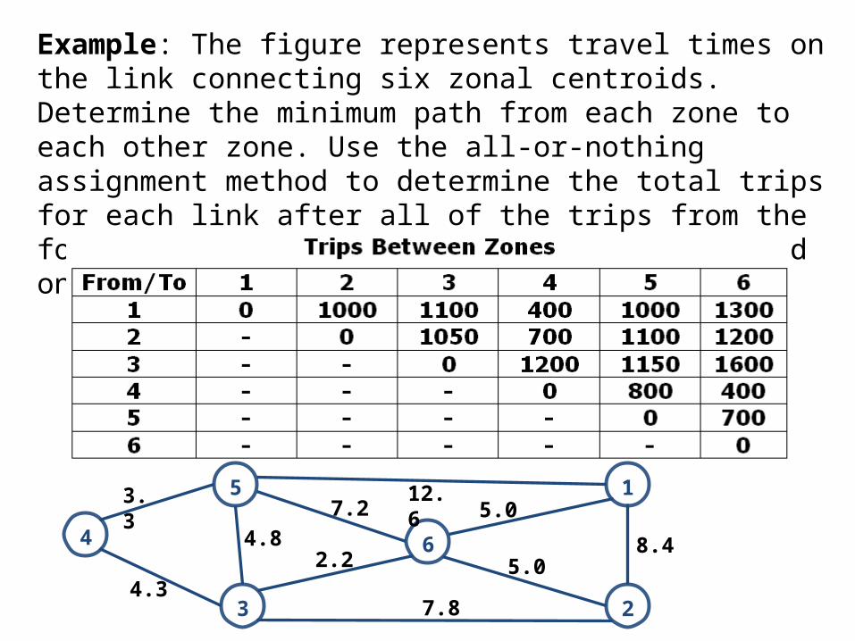
Example: The figure represents travel times on the link connecting six zonal centroids. Determine the minimum path from each zone to each other zone. Use the all-or-nothing assignment method to determine the total trips for each link after all of the trips from the following two-way trip table have been loaded onto the network.

5

4

3

6

2

13.3 12.6

5.0

5.0

8.4

4.37.8

2.2

7.2

4.8

15

2

4 6

3

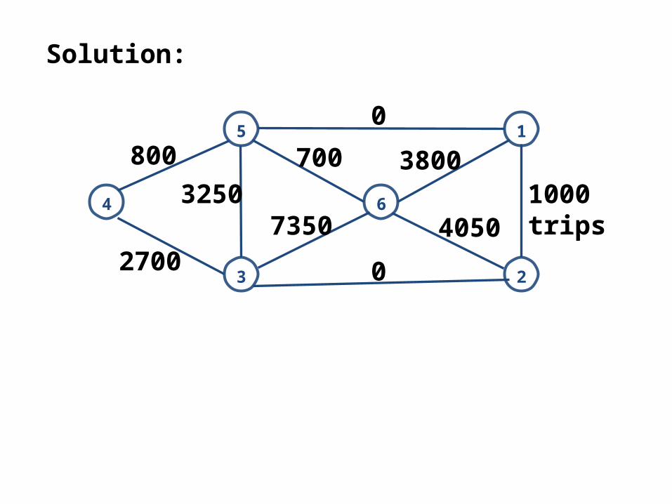
Solution:

2700

32503800

4050

0

1000 trips700

7350

800

0

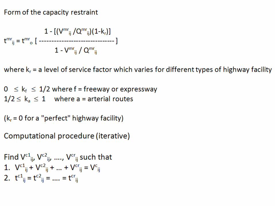
2. Minimum Path with Capacity Restraint

• Capacity-restraint techniques are based on the findings that as the traffic flow increases, the speed decreases.• There is a relationship between impedance and flow for all types of highways.• Capacity restraint attempts to balance the assigned volume, the capacity of a facility, and the related speed

Bureau of Public Roads (BPR) method

This traffic-flow-dependent travel-time relationship is represented by the general polynomial function:

Davidson Method

Davidson (1966) has suggested the use of an expression giving travel time relationship similar to the BPR formula:

Example:

A freeway section 10 miles long has a free-flow speed of 60 mph. Qmax = 2000 veh/hr, Q = 1000 veh/hr, = 0.1, = 0.474, and = 4, and T0 = 10min. Apply the (a) Davidson’s and BPR’s methods to find TQ.

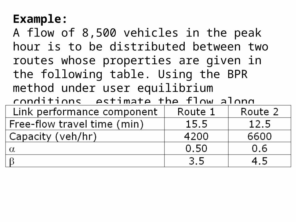
Example:A flow of 8,500 vehicles in the peak hour is to be distributed between two routes whose properties are given in the following table. Using the BPR method under user equilibrium conditions, estimate the flow along each route.

Example: A highway connecting two small cities has the following characteristics: The time (t, min) to travel on a certain stretch of a highway is t1 = 12 + 0.01q1, where q1 is the flow of vehicles (veh/hr). The demand function is q = 4800 – 100t. (a) Estimate the equilibrium flow and travel time.(b) The traffic department wants to close the existing highway and replace it with a better highway with a supply function of t2 = 12 + 0.006q2, with the same demand function. How much additional traffic will be induced by this new highway?(c) Citizens currently using the existing highway want to continue using it, and, in addition, demand the new highway as well. What will be the equilibrium flow and travel time for this scenario, assuming the demand for travel remains unchanged (Wardrop’s principle applies)?(d) If the new road is built with a supply function of t3 = 10 + 0.005t3, and the existing highway is used as well, what would be the new equilibrium flow and time?

Solution:

(c)

2

(c)

(d)

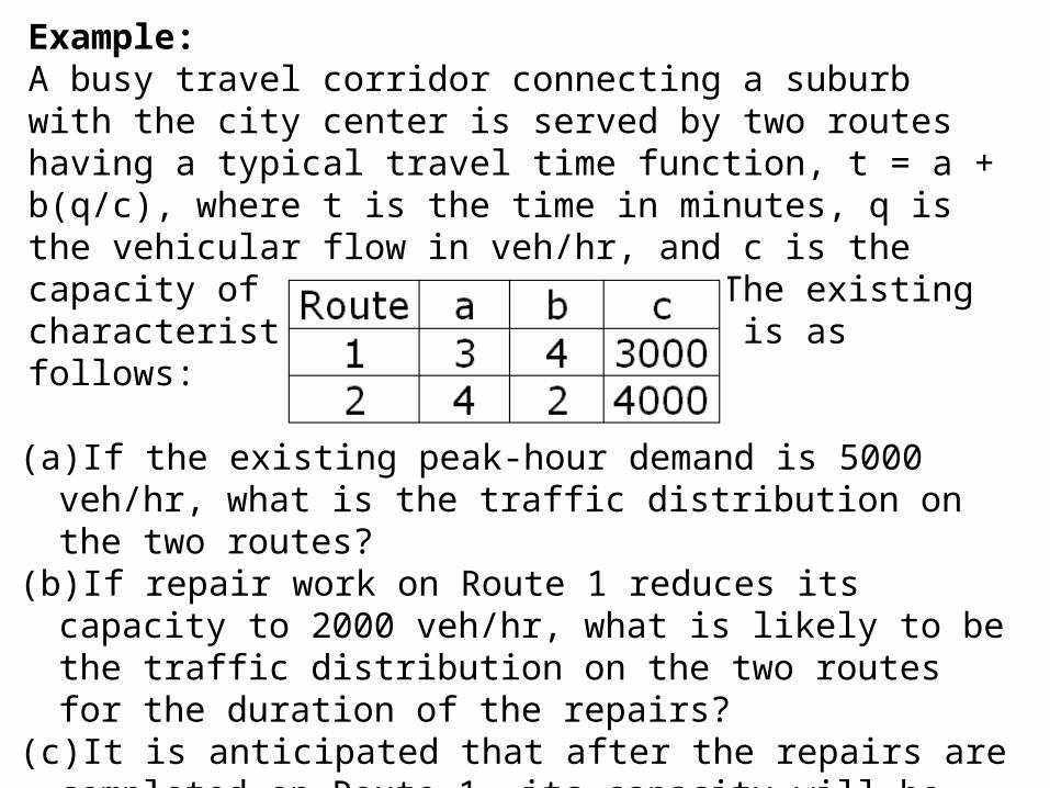
Example:A busy travel corridor connecting a suburb with the city center is served by two routes having a typical travel time function, t = a + b(q/c), where t is the time in minutes, q is the vehicular flow in veh/hr, and c is the capacity of the route in veh/hr. The existing characteristics of the two routes is as follows:

(a)If the existing peak-hour demand is 5000 veh/hr, what is the traffic distribution on the two routes?

(b)If repair work on Route 1 reduces its capacity to 2000 veh/hr, what is likely to be the traffic distribution on the two routes for the duration of the repairs?

(c)It is anticipated that after the repairs are completed on Route 1, its capacity will be 4200 veh/hr. How will this affect the distribution.

Flows in Transport Networks

a.Two Links in Series

fAB = fBC; CAC = CAB + CBC

a.Two Links in Parallel

fAB = f1 + f2; C1 = C2

Note that when links are in series, we add the cost of each link to obtain the total cost.

Figure 11-17(a)

Figure 11-17(b)

Figure 11-18(a)

Figure 11-18(b)

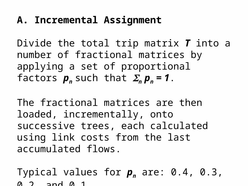
A. Incremental Assignment Divide the total trip matrix T into a number of fractional matrices by applying a set of proportional factors pn such that n pn = 1.

The fractional matrices are then loaded, incrementally, onto successive trees, each calculated using link costs from the last accumulated flows.

Typical values for pn are: 0.4, 0.3, 0.2, and 0.1. The algorithm can be written as follows:

a. Select an initial set of current link costs, usually free-flow, travel times. Initialize all flows: Va = 0; select a set of fractional pn of the trip matrix T such that n pn = 1; make n = 0.

b. Build the set of minimum cost trees (one for each origin) using the current costs; make n = n + 1.

c. Load Tn = pn T all-or-nothing to these trees, obtaining a set of auxiliary flows Fa; accumulate flows on each link:

d. Calculate a new set of current link costs based on the flows ; if not all fractions of T have been assigned proceed to step b; otherwise stop.

Disadvantages:1. This algorithm does not necessarily converge to Wardrop’s equilibrium solution.2. Incremental loading techniques suffer from the limitation that once a flow has been assigned to a link it is not removed and loaded onto another one; therefore if one of the initial iteration assigns too much flow on a link for Wardrop’s equilibrium conditions to be met, then the algorithm will not converge to the correct solutions. Advantages:1. It is easy to program.2. Its results may be interpreted as the build-up of congestion for the peak period.

Incremental Assignment

B. Method of Successive Averages Iterative algorithms were developed, at least partially, to overcome the problem of allocating too much traffic to low-capacity links.

In an iterative assignment algorithm, the “current” flow on a link is calculated as a linear combination of the current flow on the previous iteration and an auxiliary flow resulting from an all-or-nothing assignment in the present iteration.

The algorithm can be described by the following steps:

a. Select a suitable initial set of current link costs, usually free-flow travel times. Initialize all flows Va = 0; make n = 0.b. Build the set of minimum cost trees with the current costs; make n = n + 1.c. Load the whole of the matrix T all-or-nothing to these trees obtaining a set of auxiliary flows Fa.d. Calculate the current flows as:

with 0 1

e. Calculate a new set of current link costs based on the flows . If the flows (or current link costs) have not changed significantly in two consecutive iterations, stop; otherwise proceed to step b. Alternatively, the indicator could be used to decide whether to stop or not. Another, less good but quite common, criterion for stopping is simply to fix the maximum number of iterations; should be calculated in this case as well to know how close the solution is to Wardrop’s equilibrium.

Flow = 1200, Cost =21

Flow = 800, Cost =26

Solution:

Note:• The value of after iteration 10 is zero.• It can be seen that the algorithm was close to the correct equilibrium solutions in iterations 3, 6, and 9 but only reached it in iteration 10. For more realistic networks, the number of iterations needed to reach satisfactory convergences may be very high. • Fixing the maximum number of iterations is not a good approach from the point of view of evaluation. Link and total costs can vary considerably in successive iterations and this may affect the feasibility of a scheme.

Flow = 1400, Cost =22

Flow = 600, Cost =22