tropical geometry libro tesis
DESCRIPTION
Tesis sobre geometría tropicalTRANSCRIPT
Tropical Geometry
by
David E Speyer
A.B. (Harvard University) 2002
A dissertation submitted in partial satisfaction of the
requirements for the degree of
Doctor of Philosophy
in
Mathematics
in the
GRADUATE DIVISION
of the
UNIVERSITY of CALIFORNIA, BERKELEY
Committee in charge:
Professor Bernd Sturmfels, ChairProfessor Allen KnutsonProfessor Steven Evans
Spring 2005
The dissertation of David E Speyer is approved:
Chair Date
Date
Date
University of California, Berkeley
Spring 2005
Tropical Geometry
Copyright 2005
by
David E Speyer
Abstract
Tropical Geometry
by
David E Speyer
Doctor of Philosophy in Mathematics
University of California, Berkeley
Professor Bernd Sturmfels, Chair
Let K be an algebraically closed field complete with respect to a nonarchimedean
valuation v : K∗ → R. The reader should think ofK as the field of Puiseux series,
⋃∞n=1 C((t1/n)) and v as the map that assigns to a power series the exponent of
its lowest degree term. Let X be a subvariety of the torus (K∗)n. Then v(X) is
(essentially) a polyhedral complex which we term the tropicalization of X and
its combinatorial properties reflect the geometry of X .
In this thesis, we first discuss structural results about the tropicalization
of X for an arbitrary X . We then turn to the special cases of linear spaces,
Grassmannians and curves; in each case trying to describe as explicitly as possible
the possible combinatorics of the tropicalization. In the case of linear spaces, our
investigations lead us to a combinatorial theory of tropical linear spaces. This
1

theory leads to interesting combinatorial problems about matroids. In the case
of curves, the relevant combinatorial objects are “zero tension curves”. We prove
a few combinatorial results but concentrate on the other problem of determining
which zero tension curves actually occur as tropicalizations.
Professor Bernd SturmfelsDissertation Committee Chair
2

Contents
1 Introduction 1
2 General Constructions 42.1 Definitions of the Tropicalization of a Variety . . . . . . . . . . . 4
2.2 Polyhedral Structure of TropX . . . . . . . . . . . . . . . . . . . 122.3 Degenerating Toric Varieties . . . . . . . . . . . . . . . . . . . . . 16
2.4 The Tropical Degeneration and Compactifications . . . . . . . . . 202.5 The Zero Tension Condition . . . . . . . . . . . . . . . . . . . . . 34
3 The Tropical Grassmannian 37
3.1 Introduction . . . . . . . . . . . . . . . . . . . . . . . . . . . . . . 373.2 The Space of Phylogenetic Trees . . . . . . . . . . . . . . . . . . 41
3.3 The Grassmannian of 3-planes in 6-space . . . . . . . . . . . . . 48
4 Tropical Linear Spaces 534.1 Introduction and Summary . . . . . . . . . . . . . . . . . . . . . 534.2 Basic Definitions and Results . . . . . . . . . . . . . . . . . . . . 57
4.3 TropG(3, 6) and Matroidal Decompositions . . . . . . . . . . . . 694.4 Stable Intersections . . . . . . . . . . . . . . . . . . . . . . . . . . 75
4.5 Realizability of Tropical Linear Spaces . . . . . . . . . . . . . . . 824.6 Series-Parallel Matroids and Linear Spaces . . . . . . . . . . . . . 92
4.7 Special Cases of the f -Vector Conjecture . . . . . . . . . . . . . . 984.8 Results on Constructible Spaces . . . . . . . . . . . . . . . . . . . 106
4.9 Tree Tropical Linear Spaces . . . . . . . . . . . . . . . . . . . . . 122
5 Tropical Curves 1285.1 Combinatorics of Zero Tension Curves . . . . . . . . . . . . . . . 1325.2 The Bruhat-Tits Tree and Cross-Ratios . . . . . . . . . . . . . . 141
5.3 Tropical Genus Zero Curves . . . . . . . . . . . . . . . . . . . . . 1445.4 Tropical Genus One Curves . . . . . . . . . . . . . . . . . . . . . 148
i
5.5 Mumford Curves . . . . . . . . . . . . . . . . . . . . . . . . . . . 1575.6 Constructing a Tropical Curve: First Steps . . . . . . . . . . . . 1605.7 Two Lemmas . . . . . . . . . . . . . . . . . . . . . . . . . . . . . 164
5.8 Deformation of G and Z±i . . . . . . . . . . . . . . . . . . . . . . 169
Bibliography 178
ii

Acknowledgements
Throughout my study of this material, I have benefitted from the will-
ingness of many mathematicians to discuss their work and that of others with me.
I will doubtless omit some important names, but Paul Hacking, Allen Knutson,
Grisha Mikhalkin, Ezra Miller, Arthur Ogus and my advisor Bernd Sturmfels
stand out particularly. I also must thank Bernd for his guidance in editing and
planning this entire project. Finally, my thanks to Erin Larkspur, who has kept
me sane throughout the process.
iii
Chapter 1
Introduction
The fundamental observation of tropical geometry is that the solution
sets to algebraic equations, when plotted in logarithmic coordinates, look roughly
like polyhedral complexes. This behavior was first made precise in Bergman’s
paper [3] and spelled out more intuitively in Viro’s paper [46]. The aim of tropical
geometry is to make this analogy into a precise and useful tool.
In order to do this, we switch from considering the logarithm defined
on the real or complex numbers to considering a valuation on a non-archimedean
field (defined within). Now the image of the valuation will not only resemble a
polyhedral complex but will actually be one. If X denotes the solution space
of our family of equations then the image under the valuation map is called the
tropicalization of X and denoted TropX .
In the next chapter we give several descriptions of this set, prove that it
1
is indeed polyhedral, prove some of its properties and introduce a degeneration
of the solution set of the original equations whose components are indexed by
the faces of the polyhedral complex.
We then turn to applications of our theory to the fundamental examples
of algebraic geometry: linear spaces, Grassmannians and curves. In chapter 3, we
describe work of B. Sturmfels and myself to try to compute the tropicalization of
the Grassmannian Gd,n – the space of d planes in n space. We have a complete
and elegant description in the case d = 2 and we also have a complete description
of the case (d, n) = (3, 6) by direct computation.
It turns out that, just as in the classical case, the tropicalization of the
Grassmannian parameterizes the possible tropicalizations of d planes in n space
and that this is the best method for describing results about TropGd,n. We have
also found that there is a notion of “tropical linear space”, which is more general
than actual tropicalizations of linear spaces and which is purely combinatorial. In
chapter 4 we first introduce this notion, prove several equivalent characterizations
of it, and introduce combinatorial analogues of intersection and dualization. We
then discuss how actual tropicalizations of linear spaces occur among all the trop-
ical linear spaces and show that TropGd,n precisely parameterizes the collection
of tropicalizations of linear spaces.
Next, we then turn towards investigating the combinatorics of tropical
linear spaces in their own right. This section should be appealing to readers
2
who prefer combinatorics to algebraic geometry. Our main target is to prove the
“f -vector conjecture”, which describes explicitly how complicated the tropical-
ization of a d-plane in n-space can be. While we have not managed to prove the
conjecture in its full generality, we prove many special cases, including proving
it for all tropical linear spaces built out of a starting collection of hyperplanes
by repeated intersection and dualization, proving several particular cases of the
bounds and exhibiting a particularly elegant class of tropical linear spaces, the
“tree spaces”, which achieve these bounds.
In Chapter 5, we turn to the study of the tropicalizations of curves.
This field was pioneered by Mikhalkin and is to a large extent responsible for the
recent popularity of tropical thinking. We take a very different approach than
Mikhalkin and, rather than study curves via deformation of complex structure
and other symplectic techniques, we instead use Tate and Mumford’s theories of
non-archimedean uniformization. Our main result, which has been conjectured
by Mikhalkin and will appear in a future paper of his proven by quite different
methods, is that any graph in Rn which satisfies the local condition on the graph
known as the zero tension condition and a global condition called being “ordi-
nary”, which amounts to a certain matrix having full rank, actually occurs as
the tropicalization of a curve in the n-dimensional torus.
3
Chapter 2
General Constructions
2.1 Definitions of the Tropicalization of a Variety
Let K be an algebraically closed field complete with respect to a non-trivial
valuation v : K → R ∪ ∞. Recall that “non-trivial valuation” means that
v(x+ y) ≥ min(v(x), v(y))
v(xy) = v(x) + v(y)
v(0) = ∞
v(1) = 0
v(x) takes values other than 0 and ∞
Note that the second and fourth property automatically imply that, if x 6= 0 then
v(x) + v(x−1) = 0 so v(x) 6= ∞. When speaking about valuations from a ring
which is not a field, as we will have occasion to do in Theorem 2.1.2, we permit
4
DEFINITIONS OF THE TROPICALIZATION OF A VARIETY
v(x) = ∞ for nonzero x.
That K is complete with respect to v means that, if α1, α2 . . . is a
seqeunce of elements of K with limi,j→∞ v(αi−αj) = ∞ then there is an element
β of K with limi→∞ v(β − αi) = ∞.
In order to maintain compatibility with the various valued fields that
occur in mathematics, we have not assumed v to be surjective. This will cause
many technical frustrations. Our approach is to be scrupulous about handling
such issues in this chapter but to occasionally assume that relevant values are in
the image of v in later sections. This issue never has any deep effect.
We set the following notations: R will be the local ring v−1(R≥0∪∞),
M the maximal ideal v−1(R>0 ∪ ∞) of R and κ the field R/M. For most
purposes, it is best to think of K as the field⋃∞
n=1 C((t1/n)) of Pusieux series,
or as the reader’s favorite algebraically closed field of power series. It will be
convenient, however, to have the flexibility to talk about an arbitrary K.
Since K is algebraically closed, it is closed under the taking of nth roots
for all n ∈ Z. Thus, K∗ and v(K∗) are divisible groups and we can find a section
of the surjective map of groups K∗ → v(K∗). We fix such a section w 7→ tw from
v(K∗) → K∗. Explicitly, this means that tw+w′
= twtw′
and v(tw) = w. Once
again, the reader should think of the case where K is a field of power series, so
that the notation tw can simply be thought of as a monomial in K.
One notion that we will need repeatedly is the notion of an initial ideal.
5
DEFINITIONS OF THE TROPICALIZATION OF A VARIETY
Let Y be a toric variety over K with dense torus (K∗)n (we will usually be
thinking about the torus itself and almost always about the torus, affine space
or projective space), X a closed subscheme of Y and w ∈ v(K∗)n. Let Y be
the toric variety over R associated to the same fan and let X be the closure of
tw ·X ⊂ (K∗)n in Y . We define inw X = X ×R κ.
While inw X depends on the choice of t·, it does so only in a trivial
manner: a different choice of t• amounts to translating inw X by an element of
(κ∗)n. Similar comments will apply to most of our constructions.
Let f =∑
a∈A faxa be a nonzero Laurent polynomial inK[x±1
1 , . . . , x±1n ]
and let w ∈ v(K∗)n. Let W = mina∈A (∑
wiai + v(fa)), so the polynomial
t−W f(tw1x1, . . . , twnxn) is in R[x±1] and has nonzero image in κ[x±1], let inw f
be this image. Let X be a subvariety of the torus (K∗)n defined by the ideal
I ⊂ K[x±11 , . . . , x±1
n ].
Proposition 2.1.1. The ideal of inw X is spanned over κ by the polynomials
inw f as f ranges over I \ 0.
Proof. The definition of closure tells us that the ideal of inw X given by the ideal
(I ∩R[x±1 , . . . , x±n ])⊗R κ in κ[x±1
1 , . . . , x±1n ]. Let f and W be as in the preceding
paragraph with f ∈ I \ 0; we will write W (f) when necessary. We have f ∈
R[x±] if and only ifW ≥ 0. If f ∈ R[x±] then its image in (I∩R[x±1 , . . . , x±n ])⊗Rκ
is 0 if W > 0 and is inw f if W = 0. So the ideal of inw f is by definition spanned
over κ by the polynomials inw f for which f ∈ I and W (f) = 0. But, for any
6

DEFINITIONS OF THE TROPICALIZATION OF A VARIETY
f ∈ I \ 0, W (t−W (f)f) = 0, t−W (f)f ∈ I and inw f = inw
(
t−W (f)f)
. So the
set of polynomials of the form inw f with f ∈ I \ 0 is the same as the subset of
polynomials of the form inw f with f ∈ I \ 0 and W (f) = 0.
We use the above proposition to extend the definition of inwX to the
case where w 6∈ v(K∗).
Let X ⊂ (K∗)n be a closed subvariety of the torus with I(X) ⊂
K[x±11 , . . . , x±1
n ] the corresponding ideal. In the remainder of this section, we
will define four subsets of v(K∗)n and prove that they are equal. We will then
define TropX to be the closure of these sets in Rn.
Theorem 2.1.2. The following subsets of v(K∗)n are equal:
1. The set of all (v(u1), . . . , v(un)), where (u1, . . . , un) ∈ X(K).
2. The set of all points of v(K∗)n of the form (v(x1), . . . , v(xn)) where v :
O(X) → R ∪ ∞ is a valuation extending v.
3. The set of all w ∈ v(K∗)n such inw f is not a monomial for any f ∈
I(X) \ 0.
4. The set of all w ∈ v(K∗)n such that inw X 6= ∅.
Proof. We provisionally term these sets T1, T2, T3 and T4 and proceed to show
that T1 ⊆ T2 ⊆ T3 ⊆ T4 ⊆ T1.
T1 ⊆ T2: Define v by v(f) = v(f(u1, . . . , un)) for every f ∈ O(X) =
K[x±]/I(X).
7
DEFINITIONS OF THE TROPICALIZATION OF A VARIETY
T2 ⊆ T3: Suppose that w ∈ T2. Let f =∑
a∈A faxa ∈ I(X)\ 0, let v be
a valuation O(X) → R ∪ ∞ extending v with wi = v(xi). In O(X), we have
f(x1, . . . , xn) = 0 which means that the minimum of the numbers v (faxa11 · · ·xan
n )
is not unique. But
v(faxa11 · · ·xan
n ) = v(fa) +∑
aiv(xi) = v(fa) +∑
aiwi,
so saying that the minimum of this quantity as a ranges over A is not unique is
exactly saying that inw f is not a monomial.
T3 ⊆ T4: Suppose that w 6∈ T4. By the Nullstellensatz, to say that
inw X 6= ∅ is to claim that inw I(X) 63 1. Suppose that 1 ∈ inw I(X), and
write 1 =∑r
i=1 inw fi for f i =
∑
a∈Aif iax
a ∈ I(X). For each i, set Wi =
mina∈Ai(v(fa) +
∑
aiwi), so F :=∑r
i=1 t−Wif i ≡ 1 mod M. Then inw F = 1,
so w 6∈ T3.
T4 ⊆ T1: This is the only difficult part. Recall our definition of X as
the closure in the torus over R of twX ⊂ (K∗)n, and inw X as the fiber of X
over κ. We have assumed that inw X 6= ∅, let (u1, . . . , un) ∈ inw X . We must
prove there is a point (x1, . . . , xn) ∈ X with v(xi) = wi. We actually prove the
following stronger result:
Lemma 2.1.3. If w ∈ v(K∗)n and (u1, . . . , un) is a point of inw X then there is
a point (u1, . . . , un) ∈ X with ui = uitwi + higher order terms.
This result resembles Hensel’s lemma, but allows us to treat more gen-
eral varieties at the expense of treating less general fields. Hensel’s lemma has as
8
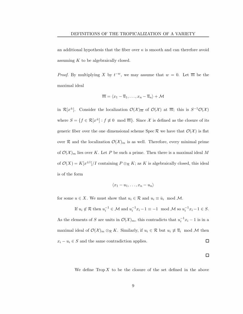
DEFINITIONS OF THE TROPICALIZATION OF A VARIETY
an additional hypothesis that the fiber over κ is smooth and can therefore avoid
assuming K to be algebraically closed.
Proof. By multiplying X by t−w , we may assume that w = 0. Let m be the
maximal ideal
m = 〈x1 − u1, . . . , xn − un〉 + M
in R[x±]. Consider the localization O(X )m of O(X ) at m; this is S−1O(X )
where S = f ∈ R[x±] : f 6≡ 0 mod m. Since X is defined as the closure of its
generic fiber over the one dimensional scheme SpecR we have that O(X ) is flat
over R and the localization O(X )m is as well. Therefore, every minimal prime
of O(X )m lies over K. Let P be such a prime. Then there is a maximal ideal M
of O(X) = K[x±1]/I containing P ⊗R K; as K is algebraically closed, this ideal
is of the form
〈x1 − u1, . . . , xn − un〉
for some u ∈ X . We must show that ui ∈ R and ui ≡ ui mod M.
If ui 6∈ R then u−1i ∈ M and u−1
i xi−1 ≡ −1 mod M so u−1i xi−1 ∈ S.
As the elements of S are units in O(X )m, this contradicts that u−1i xi − 1 is in a
maximal ideal of O(X )m ⊗R K. Similarly, if ui ∈ R but ui 6≡ ui mod M then
xi − ui ∈ S and the same contradiction applies.
We define TropX to be the closure of the set defined in the above
9
DEFINITIONS OF THE TROPICALIZATION OF A VARIETY
theorem in Rn. If we are given X in a toric variety over K, we write TropX
as shorthand for Trop (X ∩ (K∗)n). TropX seems to have first been defined
in Bergman’s paper [3]. Bergman deals with the constant coefficient case and
first gives a definition in terms of the amoeba of X , which he then relates to
a modification of definition T2 above. Bieri and Groves, in [6], used essentially
definition T2 over a general valued field.
Our order of definitions: first defining a subset of v(K∗)n and then
defining TropX as its closure in Rn leaves the possibility that there are points of
TropX ∩ v(K∗)n which do not meet the conditions of the above theorem. The
proposition below shows that there are no ambiguities of this sort.
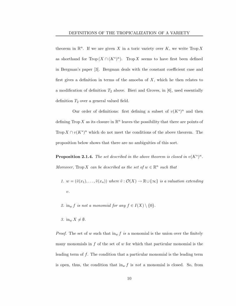
Proposition 2.1.4. The set described in the above theorem is closed in v(K∗)n.
Moreover, TropX can be described as the set of w ∈ Rn such that
1. w = (v(x1), . . . , v(xn)) where v : O(X) → R∪∞ is a valuation extending
v.
2. inw f is not a monomial for any f ∈ I(X) \ 0.
3. inwX 6= ∅.
Proof. The set of w such that inw f is a monomial is the union over the finitely
many monomials in f of the set of w for which that particular monomial is the
leading term of f . The condition that a particular monomial is the leading term
is open, thus, the condition that inw f is not a monomial is closed. So, from
10

DEFINITIONS OF THE TROPICALIZATION OF A VARIETY
Definition 3 of Theorem 2.1.2, we see that the set defined in the above theorem
is closed in v(K∗)n and that (2) above characterizes TropX .
The proof that T3 ⊆ T4 above also shows that (2) implies (3). It is even
easier to show that (3) implies (2): If inw f is a monomial for some f ∈ I then,
since monomials are units in κ[x±], the ideal of inw X is (1) and inw X is empty.
Finally, suppose that w ∈ TropX . We can extend K to a field L
with valuation such that w ∈ v(L∗)n. (Proof: make a degree n transcendental
extension K(u1, . . . , un) of K and set v(∑
aIuI) = minI(v(aI)+ < u,w >) where
aI ∈ K. It is not hard to check that this is multiplicative, and hence has a
well defined extension to the fraction field, and that the extended v is still a
valuation.) Replacing I with I ⊗K L will not change the truth of condition 3 in
the previous theorem, so wi = xi for some (x1, . . . , xn) ∈ X(L). Then we can
define v : O(X) → R by f → v(f(x1, . . . , xn)).
The characterization of TropX in terms of the set of all valuations
extending v will not be used in the future. I include it because it shows
Proposition 2.1.5. TropX is a continuous surjective image of the analytic space
associated to X in the sense of Berkovich [4].
Proof. The points of this space are, by definition, the norms on X extending
the norm e−v(·) on K. There is a bijection between valuations and norms by
v → e−v(·) where we take e−∞ = 0. The functions e−v(·) → v(xi), for 1 ≤ i ≤ n,
are continuous.
11
POLYHEDRAL STRUCTURE OF TropX
This observation (using the language of Tate’s rigid analytic spaces
rather than Berkovich’s analytic spaces) is used in [17]. I think that there is a
good opportunity for cross fertilization between the tropical and analytic geome-
try communities, as tropical geometry has not yet developed the sort of abstract
geometrical theory the analytic scholars have and, as far as I have found, the
analytic community is not utilizing the polyhedral nature of TropX .
2.2 Polyhedral Structure of TropX
Let Y be the torus (K∗)n, the affine space Kn or the projective space PnK and X
a closed subscheme of Y . We will say that a polyhedral subdivision Σ of Rn is
adapted to X if, whenever w and w′ lie in the relative interior of the same face
of Σ, we have inw X = inw′ X . The main result of this section is
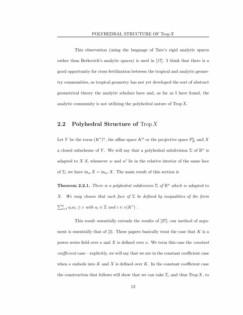
Theorem 2.2.1. There is a polyhedral subdivision Σ of Rn which is adapted to
X. We may choose that each face of Σ be defined by inequalities of the form
∑ni=1 aiwi ≥ c with ai ∈ Z and c ∈ v(K∗) .
This result essentially extends the results of [27]; our method of argu-
ment is essentially that of [2]. These papers basically treat the case that K is a
power series field over κ and X is defined over κ. We term this case the constant
coefficient case – explicitly, we will say that we are in the constant coefficient case
when κ embeds into K and X is defined over K. In the constant coefficient case
the construction that follows will show that we can take Σ, and thus TropX , to
12
POLYHEDRAL STRUCTURE OF TropX
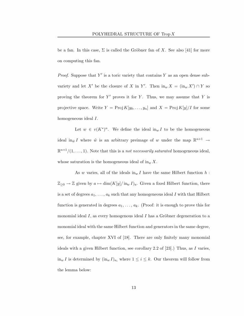
be a fan. In this case, Σ is called the Grobner fan of X . See also [41] for more
on computing this fan.
Proof. Suppose that Y ′ is a toric variety that contains Y as an open dense sub-
variety and let X ′ be the closure of X in Y ′. Then inw X = (inw X′) ∩ Y so
proving the theorem for Y ′ proves it for Y . Thus, we may assume that Y is
projective space. Write Y = ProjK[y0, . . . , yn] and X = ProjK[y]/I for some
homogeneous ideal I .
Let w ∈ v(K∗)n. We define the ideal inw I to be the homogeneous
ideal inw I where w is an arbitrary preimage of w under the map Rn+1 →
Rn+1/(1, . . . , 1). Note that this is a not necessarily saturated homogeneous ideal,
whose saturation is the homogeneous ideal of inw X .
As w varies, all of the ideals inw I have the same Hilbert function h :
Z≥0 → Z given by a 7→ dim(K[y]/ inw I)a. Given a fixed Hilbert function, there
is a set of degrees a1, . . . , ak such that any homogeneous ideal I with that Hilbert
function is generated in degrees a1, . . . , ak . (Proof: it is enough to prove this for
monomial ideal I , as every homogenous ideal I has a Grobner degeneration to a
monomial ideal with the same Hilbert function and generators in the same degree,
see, for example, chapter XVI of [18]. There are only finitely many monomial
ideals with a given Hilbert function, see corollary 2.2 of [23].) Thus, as I varies,
inw I is determined by (inw I)aiwhere 1 ≤ i ≤ k. Our theorem will follow from
the lemma below:
13
POLYHEDRAL STRUCTURE OF TropX
Lemma 2.2.2. Let V = KM be a finite dimensional K vector space of dimension
M equipped with an action of (K∗)n; choose an eigenvector decomposition V =
⊕Mi=1Kvi with vi an eigenvector of character χi for this action. For U a subspace
of V , let U0 ⊂ κM be defined by (U ∩⊕
Rvi)⊗R κ. As w varies through v(K∗)n,
the vector space (twU)0 only takes on finitely many values and, partitioning Rn
into equivalence classes by the value of (twU)0, these classes are the relatives
interiors of the faces of a polyhedral complex.
This lemma proves our result by taking V = K[y]aiand U = Iai
and
then taking the simultaneous refinement of the resulting polyhedral complexes.
Proof. Write D for the dimension of U . Note that the Plucker coordinates of
U0 in the basis vi are given by pi1···iD(U0) = 0 if v(pi1···iD(U)) is not minimal
among all valuations of Plucker coordinates of U and, pi1 ···iD(U0) = p where
pi1···iD(U) = tW p+· · · for someW if pi1···iD(U) is one of these Plucker coordinates
of minimal valuation. The Plucker coordinates of tw · U are given by pi1 ···iD(tw ·
U) = tPD
r=1<χi,w>pi1···iD(U). We thus see that the Plucker coordinates of (tw ·U)0
depend only on which of the valuations v(pi1···iD(tw ·U)) = v(pi1···iD)(U)+∑D
r=1 <
χi, w > is minimal. As a subspace is determined by its Plucker coordinates, we see
that (tw ·U)0 is determined solely by the linear inequalities comparing the values
v(pi1···iD)(U) +∑D
r=1 < χi, w > as (i1, . . . , iD) varies. Thus, the equivalence
classes form a polyhedral subdivision of Rn (and, in fact, a coherent one). In
the constant coefficient case, all of the v(pi1...iD) terms are 0 or ∞ so are the
14
POLYHEDRAL STRUCTURE OF TropX
inequalities have no constant term and we get a fan.
The next lemma, which we will use repeatedly, says that the local ge-
ometry of TropX can be reduced to the constant coefficient case.
Proposition 2.2.3. Let κ((t))alg denote the algebraic closure of the Laurent
series field over κ. Let X be a subvariety of (K∗)n and w ∈ Rn. Then the link of
TropX at w is Trop(
inw X ⊗k κ((t))alg)
. More specifically, for any u ∈ Rn we
have inw+εu X = inu
(
inw X ⊗k κ((t))alg)
for ε > 0 and sufficiently small.
Proof. The second claim implies the first because u ∈ linkw TropX if and only
if inw+εu X 6= ∅ for ε > 0 sufficiently small and u ∈ Trop(
inw X ⊗k κ((t))alg)
if
and only if inu
(
inw X ⊗k κ((t))alg)
6= ∅.
As in the proof above, complete (K∗)n to projective space and abuse
notation by writing the compactified X as ProjK[y0, . . . , yn]/I . Then the ideal
inu
(
inw X ⊗k κ((t))alg)
is finitely generated by elements of the form inu inw f
with f ∈ I . (Technically, this should be inu ι(inw f) where ι is the injection of
k[y0, . . . , yN ] into κ((t))alg[y0, . . . , yn].) Let inu inw f1, . . . , inu inw fm generate
inu inw I , for fj ∈ I . Then, for ε small enough, we will have inw+εu fj = inu inw fj
for every j. Thus, for such an ε we have inw+εu I ⊇ inu inw I . But both ideals
have the same Hilbert function, so they are equal.
15
DEGENERATING TORIC VARIETIES
Proposition 2.2.4. Suppose w ∈ TropX is contained in the relative interior of
a face σ of Σ, where Σ is adapted to TropX. Let H(σ) be the translation to the
origin of the affine linear space spanned by σ. Then inw X is invariant under
translation by the torus exp(H(σ)).
Proof. Let v ∈ H(σ), then for small ε we have inw+εv X = inwX . Using the
previous lemma, we see that, for any f ∈ inw I , we also have inv f = inv inw f =
inw+εv f = inw f . Thus, the terms of f which have lowest weight in the v-grading
again lie in inw I . Subtracting them off and repeating, we may conclude that
inw I is homogeneous with respect to the v grading. This is equivalent to being
invariant under the torus exp(Rv).
2.3 Degenerating Toric Varieties
The construction in this section appears to have been discovered several times,
the earliest reference I can find is [35]. We repeat it here as it does not appear
to be well known. Let Σ be a (finite) polyhedral complex in Rn whose faces are
defined by inequalities of the form∑
aixi ≥ w with ai ∈ Z and w ∈ v(K∗).
Define Σ1 to be the fan whose cones are the recession cones of the faces of Σ.
We will construct, associated to Σ, a flat family T over SpecR whose fiber over
SpecK is the toric variety T assosciated to Σ1 and whose fiber over Spec κ is a
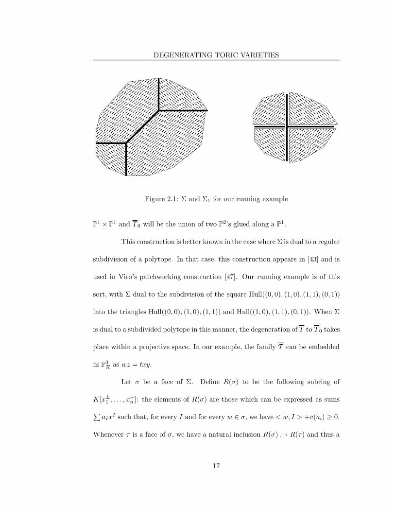
union of toric varieties T 0 indexed by the faces of Σ. As a running example, we
will take the case where Σ is the complex in R2 shown in Figure 2.1. T will be
16
DEGENERATING TORIC VARIETIES
Figure 2.1: Σ and Σ1 for our running example
P1 × P1 and T 0 will be the union of two P2’s glued along a P1.
This construction is better known in the case where Σ is dual to a regular
subdivision of a polytope. In that case, this construction appears in [43] and is
used in Viro’s patchworking construction [47]. Our running example is of this
sort, with Σ dual to the subdivision of the square Hull((0, 0), (1, 0), (1, 1), (0, 1))
into the triangles Hull((0, 0), (1, 0), (1, 1)) and Hull((1, 0), (1, 1), (0, 1)). When Σ
is dual to a subdivided polytope in this manner, the degeneration of T to T 0 takes
place within a projective space. In our example, the family T can be embedded
in P3R as wz = txy.
Let σ be a face of Σ. Define R(σ) to be the following subring of
K[x±1 , . . . , x±n ]: the elements of R(σ) are those which can be expressed as sums
∑
aIxI such that, for every I and for every w ∈ σ, we have < w, I > +v(ai) ≥ 0.
Whenever τ is a face of σ, we have a natural inclusion R(σ) → R(τ) and thus a
17
DEGENERATING TORIC VARIETIES
natural map SpecR(τ) → SpecR(σ) which turns out to be an inclusion. Gluing
the latter as in the standard construction of a toric variety, we build T .
In our example, the vertices at (0, 0) and (1, 1) correspond to the rings
R[x±1 , x±2 ] and R[(t−1x1)
±, (t−1x2)±] respectively. The spectrum of each of these
rings is a flat family over SpecRwith general and special fibers each n-dimensional
tori. Because (0, 0) and (1, 1) both correspond to the same face of Σ1 (the origin)
their general fibers are glued together, but their special fibers, which correspond
to different faces of Σ, are not. The edge running from (0, 0) to (1, 1), which
we will denote e, corresponds to the ring R[x±1 , x±2 ] ∩ R[(t−1x1)
±, (t−1x2)±] =
R[(x1x−12 )±, x1, tx
−11 ]. This can also be written as R[u±, v, w]/(vw− t). This
ring corresponds to a family over SpecR whose fiber over K is SpecK[u±, v±] =
(K∗)n and whose fiber over κ is Spec κ[u±, v, w]/(vw), which is two copies of
κ∗ × κ glued along a κ∗. The inclusions of the two endpoints of this segment
into this segment correspond to inclusions of R((0, 0)) and R((1, 1)) into R(e).
In each of these inclusions, the map on fibers over K is an isomorphism and the
map on fibers over κ takes (κ∗)2 into one of the two copies of κ∗ × κ. Adding
in the patches from the other faces of Σ, we get a family whose fiber over K is
P1K × P1
K and whose fiber over κ is two copies of P2κ glued along a P1
κ.
We now return to discussing our general construction. Let T denote
T ⊗R K and T 0 denote T ⊗R κ. Using ∂T for the toric boundary of T and
∂T 0 for its closure in T0, let T0 = T 0 \ ∂T0. So T0 is a flat degeneration of
18

DEGENERATING TORIC VARIETIES
the torus (K∗)n and T and T0 are partial compactifications of (K∗)n and T0
respectively. We will sometimes denote (K∗)n as T to be consistent with the rest
of this notation.
For σ ⊂ Rn a polytope, let H(σ) denote the translation to the origin
of the affine linear space spanned by σ. There are natural actions of (K∗)n and
(κ∗)n on T and T 0 respectively such that the orbits are in bijection with the
faces of Σ1 and Σ respectively. This correspondence is inclusion reversing on
the closures and the orbit Oσ corresponding to a face σ has stabilizer expH(σ).
Note that, as with a standard toric variety, the following potentially confusing
point exists: each face σ ∈ Σ corresponds to a coordinate patch SpecR(σ)⊗R κ
on T0. This patch is⋃
τ⊆σ Oτ . The assignment of patches to faces is inclusion
preserving; that of orbits to faces is inclusion reversing.
We will need the following lemma often in the future:
Lemma 2.3.1. Let w ∈ v(K∗)n and suppose that w lies in the relative interior
of σ ⊂ Rn where σ is a face of Σ. Consider the point tw ∈ (K∗)n ⊂ T . Then the
limit of tw in T 0 lies in the torus orbit corresponding to σ.
Proof. We may do this computation while looking solely at the coordinate patch
SpecR(σ). Define a map R(σ) → R by∑
aIxI 7→
∑
aI t<w,I>. By the definition
of R(σ) and the assumption that w ∈ σ, the image truly lands in R (and not
just K). By definition, over K, this is the inclusion of the point tW into (K∗)n.
Thus, the limit of tw does lie somewhere in SpecR(σ) ⊗R κ and must lie in the
19
THE TROPICAL DEGENERATION AND COMPACTIFICATIONS
orbit Oτ for some τ ⊆ σ. Thus it is enough to show that the limit of tw is not
in the coordinate patch corresponding to τ for any τ ) σ.
Let τ ) σ. Since w is in the relative interior of σ, we know that w 6∈ τ
and we can find an affine linear functional∑
aixi+v which is 0 on τ but negative
at w. Then tvxa11 · · ·xan
n is a monomial that is in R(τ). Evaluating this monomial
at xi = twi produces a negative power of t and thus not a member of R. So the
map R(σ) → R by evaluation at xi = twi can not be extended to a map R(τ) →
R. The corresponding geometric statement is that the map SpecR → SpecR(σ)
which sends SpecK to tw does not factor through SpecR(τ).
2.4 The Tropical Degeneration and Compactifications
Let X ⊂ (K∗)n and let Σ ⊂ Rn be a polyhedral complex. In the previous section,
we defined the family T over SpecR, with generic fiber a toric variety T and
special fiber T 0. We define X to be the closure of X in T , X0 to be the closure
of X in T0 and X0 be the closure of X in T0; we have X0 = X0 ∩ T0. We will
refer toX , X0 andX0 as the “tropical compactification”, “tropical degeneration”
and “compactified tropical degeneration” of X , respectively. These constructions
make sense for any Σ, but their importance arise when Σ is supported on TropX
and sufficiently fine. In this case, we will see that X0 is covered by strata indexed
by the faces of Σ and isomorphic to quotients by tori of the various inw X .
20
THE TROPICAL DEGENERATION AND COMPACTIFICATIONS
Before continuing with the general theory, we pause to work out the
example of the hypersurface X given by t+x+ y +xy = 0 in (K∗)2. The special
case whereX is a hypersurface is central in the Patchworking construction of Viro
([47]) and in the work of Gelfand, Kapranov and Zelevinsky ([21]). Sturmfels has
generalized Viro’s work to complete intersections in [44].
With X = (x, y) : t+ x+ y + xy = 0, it is easy to check that TropX
is the one skeleton of the polyhedral complex Σ in Figure 2.1. We saw in the
previous section that the polyhedral complex in Figure 2.1 corresponded to a copy
of P1 ×P1 over K degenerating to two copies of P2 over κ. Taking the 1-skeleton
of Σ corresponds to removing the four torus fixed points from each fiber. Let e
denote the diagonal edge of Σ. The edge e corresponds, as we saw in the last
section, to a coordinate patch SpecR[(xy−1)±, x, tx−1] = SpecR[u±, v, w]/(vw−
t). The ideal of X inside this coordinate patch is found by intersecting the ideal
(t + x + y + zx) in K[x±, y±] with R[(xy−1)±, x, tx−1]. The resulting ideal is
generated by x−1(t+ x+ y + xy) = tx−1 + 1 + (xy−1)−1 + x(xy−1)−1. In terms
of the (u, v, w) variables, this is v + 1 + u−1 + wu−1.
Consider the coordinate patch SpecR[u±, v, w]/(vw− t); its fiber over
κ is Spec κ[u±, v, w]/(vw). Geometrically, this is two copies of κ×κ∗ glued along
a κ∗. The ideal of X0 inside this coordinate patch (actually, only X0 meets this
patch) is cut out by v + 1 + u−1 + wu−1. This cuts out a rational curve in each
component of Spec κ[u±, v, w]/(vw), given by v+1+u−1 = 0 and 1+u−1 +wu−1
21
THE TROPICAL DEGENERATION AND COMPACTIFICATIONS
respectively. Note that the intersections of these curves with (κ∗)2 are in(0,0) and
in(1,1)X . The intersection of X0 with the orbit Oe = Spec κ[u±] is given by the
ideal (u−1 + 1). Note that this is the quotient of in(s,s)X by its invariant torus
for any s ∈ e.
This construction was discovered by Tevelev in the constant coefficient
case, see [45], and also partially and in a messier form by myself. Hacking realized
that this construction could be used to study the cohomology of Trop(X) \ 0.
It seems not to have been defined before for the nonconstant coefficient case.
This section has benefited greatly from conversations with P. Hacking.
Proposition 2.4.1. X0 and X0 are flat degenerations of X and X respectively.
If we assume that the support of Σ contains TropX, then X and X0 are proper
over K and κ respectively.
Proof. X0 and X0 are both defined as the fibers over Spec κ of the closures of X
and X within the flat families T \∂T and T ; this proves the first claim. Complete
Σ to a polyhedral complex Σ′ whose support is all of Rn; let T′etc. denote the
associated objects. T′is a proper toric variety, as it is associated to a complete
fan and, similarly, T′0 is proper because it is a union of toric varieties each of
which is given by a complete fan. X′and X
′0 are similarly proper because they
are closed subvarieties of T′and T
′0 respectively.
We will show that, in fact, X′= X and X
′0 = X0. Let σ be a face of
Σ′ not in Σ and let Oσ be the corresponding orbit in T′0. We will show that the
22
THE TROPICAL DEGENERATION AND COMPACTIFICATIONS
closure of X is disjoint from Oσ . Repeating this for every such σ shows that X′0
in fact lies entirely in T0 and thus is X0.
Every point of the closure of X can be approached along a one dimen-
sional path through X . More precisely, let D be Spec S for S some discrete valu-
ation ring with fraction field L, residue field λ and uniformizer u. Let φ : D → T′
with φ(SpecL) ∈ X . We want to show that φ(λ) 6∈ Oσ; we will then know that
the closure of X is disjoint from Oσ. If φ(λ) lands in the fiber above SpecK then
trivially it is not in Oσ, so we are only interested in the case where φ(λ) lands
above κ. In this case, the projection from T′→ SpecR gives us a surjective map
Spec S → SpecR and we can extend v to a map L∗ → R, which we will also
denote as v. Writing xi for the coordinate functions on the big torus in which X
lives, we may now consider w := (v(φ∗(x1)), . . . , v(φ∗(xn))).We have w ∈ TropX ,
as definition 4 of TropX in Theorem 2.1.2 is clearly invariant under extending
the ground field to L. Then w is not in the relative interior of σ, as σ 6∈ Σ and
TropX is supported on Σ. So, by Lemma 2.3.1, φ(λ) is not in Oσ . We now know
that X′0 = X0 as promised and is proper.
One could use a similar argument to see thatX′= X and is thus proper.
A simpler argument is to see that D := X′\X is closed. (It is the intersection of
X with the closed subvariety of T corresponding to the faces of Σ′ and Σ′1 not it
in σ and Σ′.) Since X′is proper over SpecR the image of D in SpecR must be
closed. But we have just seen that Spec κ is not the image of D, so the image of
23
THE TROPICAL DEGENERATION AND COMPACTIFICATIONS
D is empty and thus D = ∅ and X = X′.
The idea of this paragraph is due to Tevelev and Hacking in the constant
coefficient case: Construct a family F ⊂ T ×R SpecR[x±1 , . . . , x±n ] over T as
follows: Over x ∈ (K∗)n the fiber Fx is x−1 ·X . F is then the closure of this
family in the n-torus family over T . In this setting, X can be described as
x ∈ T : (1, . . . , 1) ∈ Fx. We now show
Theorem 2.4.2. There is a choice of polyhedral structure Σ on TropX such
that F is flat over X ; for the rest of the statement of this theorem assume that
Σ has this property. Let x ∈ Oσ for σ ∈ Σ. Oσ contains a canonical point x0
which is the flat limit of tw for every w in the relative interior of σ. Let x = sx0
for s ∈ (κ∗)n, then the fiber of F over x is s−1 · inw X.
Proof. Let I ⊂ K[x±] be the ideal of X and take a provisional choice of Σ fine
enough to be adapted to X .
Lemma 2.4.3. Fix σ ∈ Σ and let J = inw I for w in the relative interior of σ.
Let f be a polynomial in J which is homogeneous and of degree 0 with respect to
the action of exp(H(σ)). There is a finite collection g1, . . . , gr of members of I
such that, for every w in the interior of σ we have inw gi = f for some 1 ≤ i ≤ r.
In the constant coefficient case, we could simply take Σ fine enough to
be adapted to the closure of X in Pn. Then we could construct such gi from a
24
THE TROPICAL DEGENERATION AND COMPACTIFICATIONS
universal Grobner basis. We prefer to give a direct proof rather than to adapt the
proof of the existance of a universal Grobner basis to the non-constant coefficient
case.
Proof of Lemma 2.4.3. We first summarize the strategy of our proof. Consider
some w in the relative interior of σ. There is a gw ∈ I such that inw gw = f .
Moreover, there will be an open subset Uw of σ containing w such that inw′ gw = f
for w′ ∈ U . If the relative interior of σ were compact, we would then be able to
take a finite number of Uw’s covering the relative interior of σ and the assosciated
gw’s would satisfy the claim.
Unfortunately, the relative interior of σ is not compact. Therefore, we
impose a condition on w′ which is a bit more complicated than simply asking that
inw′ gw = f so that we can work with w on the bondary of σ. Secondly, σ may
also not be compact. We counter this by taking the cone on σ and intersecting
it with the unit sphere. It is simplest to present both modifications at once.
Embed σ into Rn×R≥0 and let σ be the closed cone over σ. Let (w, e) ∈
Rn × R≥0 and let f =∑
E∈A fEXE ∈ K[x±]. We define in(w,e) f as follows: for
e > 0 we put in(w,e) f = in(w/e) f and for e = 0 we put in(w,0)(∑
I∈A fExE) =
∑
E∈B fExE where B is the subset of A on which < w,E > is maximized. Note
that in(w,e) f ∈ κ[x±] for e > 0 and in(w,0) f ∈ K[x±]. Note that, given f ∈ K[x±]
and (w1, e1), (w2, e2) ∈ Rn×R≥0, we have in(w1,e1) in(w2 ,e2) f = in(εw1+w2 ,εe1+e2) f
for ε > 0 sufficiently small. (Here, when e2 > 0, the left hand side is techinically
25
THE TROPICAL DEGENERATION AND COMPACTIFICATIONS
in(w1,e1) ι(in(w2,e2) f) where ι is the obvious embedding κ[x±] → κ((t))alg[x±].)
Also, note that we have in(w,e) f = in(λw,λe) f for λ ∈ R>0.
Our proof is by induction on D = dim σ+ ε where ε = 0 if we are in the
constant coefficients case and 1 otherwise.
Let (w, e) ∈ σ, (w, e) 6= (0, 0). We claim that there is an open neigh-
borhood U of (w, e) in σ a finite number of polynomials g1, . . . , gr such that,
for every (w′, e′) in the intersection of U and the relative interior of σ, we have
in(w′,e′) gi = f for some gi. Let us see why this finishes the proof: Since in(w′,e′) is
invariant under scalaing (w′, e′), we may assume that U is homothety invariant.
The intersection of σ with the sphere of radius 1 is compact, so we may cover σ
with a finite number of these U . Then the union of the finite number of finite
collections of g’s meets the conditions of the theorem.
We now must prove the claim of the previous paragraph. Let τ be the
face of σ containing (w, e). We have dim τ ≥ 1. Let Iτ = in(w,e) I . Then Iτ is
homogenous with respect to exp(H(τ) ∩ Rn). Let Q denote the cone of vectors
(u, d) such that (w, e)+ε(u, d) ∈ σ for ε > 0 small enough. The ideal Iτ is defined
over the ring R of polynomials homogenous with respect to exp(H(τ)∩Rn); write
I ′ for Iτ ∩ R. (R might be either a polynomial ring defined over κ or over K
depending on whether τ is in Rn × 0 or not, we are trying to emphasize the
similarity of the two cases.) Since J is homogenous with respect to exp(H(σ)) ⊇
exp(H(τ)∩ Rn), J ′ is also generated over R; let J ′ be J ∩ R.
26

THE TROPICAL DEGENERATION AND COMPACTIFICATIONS
We want to apply our inductive hypothesis with I ′, J ′ and Q/(H(τ)∩
Rn) in place of I , J and σ. If τ is contained in Rn then H(τ) ∩ Rn is at least 1
dimensional so transferring our attention to Q/(H(τ)∩Rn) reduces D by 1. If we
are not already in the constant coefficients case when considering I then we are
when considering I ′ so again D is reduced by 1. Finally, if we were already in the
constant coefficients case when considering I then Σ was a fan and everything is
invariant under scaling Rn×R≥0 both only along the first n coordinates and only
along the last coordinate. This allows us to replace the use of the unit sphere by
the unit sphere in Rn × 1, which only meets τ when τ ∩ Rn has dimension at
least 1 (i.e. τ is not the cone on the vertex of σ), so again D goes down by one.
We conclude that there is a finite number of polynomials gτ1 , . . . , gτ
r ∈ I ′
such that, for every (u, d) in the relative interior of Q, in(u,d) gτi = f for some gτ
i .
Since gτi ∈ I ′ ⊂ Iτ , each gi is in(w,e) gi for some gi ∈ I .
We first see that there is an open set U τ ⊂ τ containing (w, e) such
that in(w′,e′) gi = gτi for (w′, e′) ∈ U τ . This is simple enough: writing gi =
∑
E∈A gE,ixA, gτ
i is a sum over the subset of A on which ev(gE,i)+ < w,E > is
minimized, call this subset B. We know that gτI is homogenous for exp(H(τ) ∩
Rn), which means that < w′, E > is constant on B for w′ ∈ H(τ)∩Rn. Thus, as
(w′, e′) moves through τ , e′v(gE,i)+ < w′, E > remains constant on B. We just
have to make sure that this constant value is still the minimum, which amounts
to a finite list of inequalities.
27
THE TROPICAL DEGENERATION AND COMPACTIFICATIONS
By shrinking U τ , we may arrange that the closure of U τ is compact,
contained in the relative interior of τ and that inw′,e′ gi = gτi also holds for
(w′, e′) in this closure. Now, for every (u, d) in the relative interior of τ and every
(w′, e′) ∈ U τ , there is an i such that in(u,d) in(w′,e′) gi = f . For ε > 0 small enough
, we have
in(u,d) in(w′,e′) gi = inε(u,d)+(w′,e′) gi.
Let us restrict (u, d) to range over those vectors in the relative interior of τ
whose components are all less than 1. We claim that we can choose ε uniformly,
independent of (u, d) (subject to the preceeding restriction) and (w′, e′) so that
the displayed equality holds.
Let gi =∑
E∈A gE,ixE . Let B be the subset of A on which e′v(gE,i)+ <
w′, E > is minimized for (w′, e′) ∈ U τ . Let C be the further subset of B on which
dv(gE,i)+ < u,E > is minimized. Then in(u,d) in(w′,e′) gi is a sum over C. We
will have inε(u,d)+(w′ ,e′) gi = in(u,d) in(w′,e′) gi as long as C is also the subset of A
on which (εd+ e′)gi as long as C is also the subset of A on which
(εd+e′)v(gE,i)+ < εu+e′, E >= ε(dv(gE,i)+ < u,E >)+(e′v(gE,i)+ < w′, E >)
assumes its minimum; call this subset C ′. Now, e′v(gE,i)+ < w′, E > is consant
on B, so C ′ ∩ B = C. Thus, we simply want to insure that C ′ ⊆ B or, in other
words, that |ε(dv(gE,i)+ < u,E >)| is always less than the difference between
e′v(gE,i)+ < w′, E > on B and e′v(gE,i)+ < w′, E > on A \ B. Now, we have
required that in(w′,e′) gi = gτi for (w′, e′) in the closure of U τ , so the value of
28
THE TROPICAL DEGENERATION AND COMPACTIFICATIONS
e′v(gE,i)+ < w′, E > on B is greater than its value on A \ B for all (w′, e′)
in this closure. Since we took the closure of U τ to be compact, there is some
positive lower bound for the difference between e′v(gE,i)+ < w′, E > on B and
e′v(gE,i)+ < w′, E > on A \B for all (w′, e′) ∈ U τ . On the other hand, since we
took (u, d) to be bounded, there is an upper bound for dv(gE,i)+ < u,E > and
we see that we can indeed choose ε uniformly.
Let V denote the subset of the relative interior of τ where all coordinates
are less than 1. U τ + εV is the desired U .
We now continue with our proof of Theorem 2.4.2. For every face σ ∈ Σ
and w in the relative interior of σ take a finite generating set f1, . . . , fr for inw I .
By the lemma, for each fi we can find a finite set of polynomials g1i , . . . , gsi
i
so that, for every w in the relative interior of σ we have inw gti = fi for some
1 ≤ t ≤ si. By refining Σ, we may guarantee that the following holds: for
every σ ∈ Σ there is a generating set fσi of inw I (for w in the relative interior
of σ) and a collection of polynomials gσi such that inw g
σi = fσ
i for all w in the
relative interior of σ. Moreover, we can require that fσi be homogeneous with
respect to exp(H(σ)), that the coefficient of x0 in fσi be nonzero (by multiplying
by a polynomial) and that the valuation of the coefficient of x0 in gσi be 0 (by
multiplying by a scalar).
Let gσi =
∑
E∈A gσ,iE xE and fσ
i =∑
E∈A′ fσ,iE xE. By the normalizations
at the end of the above paragraph, for every w in the relative interior of σ we have
29
THE TROPICAL DEGENERATION AND COMPACTIFICATIONS
v(gσ,iE )+< w,E > ≥ 0 and achieves the minimal value of 0. This implies that gσ
i ∈
R(σ). Now, let x ∈ Oσ and let x0 and s be as in the statement of the theorem. We
will now prove that the fiber of F over x is s−1 · inw X . We may compute in the
coordinate patch SpecR(σ)[y±1 , . . . , y±n ]. The polynomial
∑
gσ,iE xEyE is in the
ideal defining F inside (K∗)n and lies in SpecR(σ)[y±1 , . . . , y±n ] by the preceding,
so it vanishes on the restriction of F to SpecR(σ)[y±1 , . . . , y±n ]. Specializing to
yi = si and setting M = 0, we get that∑
fσ,iE sExE vanishes on the fiber of
F over x. Since the polynomials∑
fσ,iE sExE generate s−1 · inw I , we see that
Fx ⊆ s−1 inw I . On the other hand, s−1 · inw X is the flat limit of the restriction
of F to the one parameter family stw , so Fx must contain this limit and we see
that Fx = s−1 · inw X .
Finally, we must prove flatness of F . As flatness is an open condition on
the base, it is enough to show that F is flat over X0. Take x ∈ T0. By Theorem
4.2.8.a of [32] it is enough to find a collection of maps Spec Si → T from the
spectra of discrete valuation rings to T with the closed point of each Spec Si
mapping to x such that (1) the map A →∏
Si from the local coordinate ring
of T at x to the product of the Si is injective and (2) F ×T Spec Si is flat over
Spec Si. The collection of sections SpecR → T with SpecK landing in (K∗)n
and Spec κ hitting x obeys the first condition.
The map SpecK → T is given by an n-tuple (u1, . . . , un) ∈ (K∗)n. Let
wi = v(ui). The assumption that Spec κ is taken to a point of Oσ implies that
30
THE TROPICAL DEGENERATION AND COMPACTIFICATIONS
(w1, . . . , wn) := (v(u1), . . . , v(un)) is in the relative interior of σ and that, writing
ui = `itwi mod twiM for `i ∈ κ, we have (`1, . . . , `n) · x0 = x. The flat limit
of F along this family is (`1, . . . , `n)−1 times the limit along tw, which is inw X .
This completes the proof of Theorem 2.4.2.
Set Xσ = X0 ∩ Oσ , so X0 =⊔
Xσ. We now list the main properties of
the Xσ.
Proposition 2.4.4. 1. If Xσ is in the closure of Xτ then τ ⊂ σ.
2. For any σ, the union⋃
τ⊆σ Xσ is affine.
3. For any σ, the union⋃
τ⊇σ Xσ is proper.
4. Assume X is irreducible. Then Xσ is d − dimσ dimensional, where d is
the dimension of X.
Proof. (1) This just comes from the closure relation on the orbits Oσ .
(2) We first note that⋃
τ⊆σ Oσ is affine by construction. Then⋃
τ⊆σ Xσ
is a closed subvariety of that affine variety.
(3) We use the same trick as in the proof of the previous proposition.
First, complete Σ to a complete polyhedral complex Σ′. Then⋃
τ⊇σ′ Oσ′ is proper
when the union is taken over σ′ ∈ Σ′ and⋃
τ⊇σ X′σ is a closed subvariety of this
proper variety and hence is proper. But, if σ is a face of Σ′ not in Σ, then X ′σ is
empty.
31
THE TROPICAL DEGENERATION AND COMPACTIFICATIONS
(4) Let w lie in the relative interior of σ, so by Proposition 2.2.4, inw X
is invariant under exp(H(σ)). We claim that Xσ = inw X/ exp(H(σ)). We show
that inw X has dimension d, so the dimension of Xσ = d− dimH(σ). Proof that
inw X has dimension d: inw X is the intersection in SpecR[x±] of the closure of
twX and the fiber over Spec κ. The closure of twX , henceforth denoted twX , is of
dimension d+ 1 and is irreducible since it is the closure of an irreducible scheme
twX . So the intersection of twX with the fiber over Specm has dimension at
least d, and we must have equality because twX also lies over the general fiber.
(This argument is a modification of [22], first pararaph of the proof of Theorem
1.) We now check the claim.
Every point x ∈ Oσ is of the form x = s · x0 where x0 is the limit of
tw and s ∈ (κ∗)n. Note that s is determined only modulo exp(H(σ)). In the
notation of the preceding lemmas, we have Fx = s−1 · inw X and x ∈ Xσ if and
only if (1, . . . , 1) ∈ Fx. We thus see that x ∈ Xσ if and only if s ∈ inw X , so
Xσ∼= inwX/ exp(H(σ)).
Remark: We will not use the family F again, but it is very powerful.
Hacking, has observed that, if every inwX is smooth as a scheme, then it follows
that the whole family F is smooth and one can deduce that, essentially, Xσ
has normal crossing singularities. This has implications for the cohomology of
TropX , at least in the constant coefficient case, which will hopefully appear in
future work of either Hacking or Hacking and I. Even when F is not smooth,
32
THE TROPICAL DEGENERATION AND COMPACTIFICATIONS
Hacking points out in a response to a question of mine that one still has a
resolution of the structure sheaf of X0 by the structure sheaves of the Xσ.
Remark: One flaw of the preceding is that, if Xσ is disconnected and
τ ⊇ σ, it is possible that only part of Xσ lied in the closure of Xτ . However, there
are many cases where one can exclude this possibility. In the next section, we
will see that, when X is a curve, we can often deduce that the Xv are connected
simply by looking at the combinatorics of TropX and the degree of X .
As one easy application of what has proceeded, we prove the following
results which first appeared in [6] and [17].
Proposition 2.4.5. Suppose that X is pure ( e.g. irreducible) of dimension d.
Then TropX is pure of dimension d.
Proof. Let σ be a facet of Σ. Then⋃
τ⊇σ Xτ = Xσ. The left hand side is proper
and the right hand side is affine. The only schemes that are proper and affine
are the zero dimensional schemes. So we see that dimXσ = d − dimσ = 0 and
dimσ = d.
Proposition 2.4.6. Suppose that X is irreducible. Then TropX is connected.
Proof. Suppose that TropX = U t V for U and V closed and open. U and
V are necessarily subcomplexes of Σ. Since these subcomplexes are closed up-
wards,⋃
σ∈U Xσ and⋃
σ∈V Xσ are closed and disjoint subsets of X0 so X0 is
disconnected. But an irreducible subvariety X of a proper variety T can not
degenerate within a proper family to a disconnected one, a contradiction.
33

THE ZERO TENSION CONDITION
2.5 The Zero Tension Condition
Let Σ ⊂ Rn be a pure d-dimensional polyhedral complex, where every face has
rational slope and wt a map assigning a positive integer to each facet of Σ. We
call the pair (Σ, wt) a zero tension complex if the following condition is met: for
any (d − 1) dimensional face ρ of Σ (a ridge), let σ1, . . . , σr be the facets of
Σ containing ρ. The image of H(σi) in Rn/H(ρ) is a one dimensional ray with
rational slope, let vi be the minimal lattice vector along this ray. We require
that, for every ρ, we have∑
wt(σ1)vi = 0. We will often abuse notation and
refer to Σ by itself as a zero tension complex.
Theorem 2.5.1. Recall that, if σ is a facet of TropX, then X0(σ) ∼= (κ∗)d × A
for some zero dimensional scheme A. Set wt(σ) to be dimκ O(A). With this
choice of wt, the complex TropX is a zero tension complex.
Proof. Let ρ be a codimension one face of Σ. Then, by Proposition 2.2.4,Xρ = C
for some one-dimensional scheme C ⊂ (κ∗)n/ exp(H(ρ)). By Proposition 2.2.3,
the link of ρ is TropC and one can check that the weight functions wt on TropX
and TropC are consistent. Thus, we are reduced to the case of TropC for C a
curve in (κ∗)n.
In this case, TropC is a union of finitely many rays, let v1, . . . , vr be
the minimal lattice vectors along each of these rays and let wi = wt(R+vi). We
want to show that∑
wivi = 0; it is enough to show that∑
wi < vi, u >= 0 for
every u ∈ Zn. Each ray of TropC corresponds to finitely many points of C.
34

THE ZERO TENSION CONDITION
Consider the function φ : (κ∗)n → κ∗ given by (x1, . . . , xn) 7→ xu11 · · ·xun
n .
φ extends to a meromorphic function on the toric variety T 0 with a pole of order
< u, vi > at the boundary component of T0 assosciated to vi. It is easy to check
that φ extends to a meromorphic function on C with a pole of order < u, vi > at
pi. The intersection of C with this boundary component is the zero dimensional
scheme whose length is defined to be wi. So, at the points of Cσ , φ has wi< u, vi >
zeroes. Since φ has equally many zero and poles,∑
wi < vi, u >= 0.
We can now explain the remark in the previous section that we can often
rule out the possibility of the Xσ being disconnected by examining the geometry
of TropX .
Proposition 2.5.2. Suppose that X ⊂ (K∗)n is a curve and that, at every vertex
of TropX, the edges incident to that vertex have a unique linear relation between
them. Suppose furthermore that the number of unbounded rays of TropX in
direction u is equal to the degree of the function∏
xui
i on X. Then, for every
vertex v of TropX, Xv is irreducible.
Proof. Suppose for the sake of contradiction that Xv = C1 ∪C2. Then TropX =
TropC1∪TropC2 and the weights w arising fromX , C1 and C2 obey wX = wC1 +
wC2 . With the stated hypotheses, the only way to partition w into contributions
coming from C1 and C2 such that the zero tension condition is obeyed is to have
TropC1 = TropC2. But then wt(e) > 1 for each e. In particular, the unbounded
rays of TropX have weight greater than 1. Let u be a particular direction of
35
THE ZERO TENSION CONDITION
unbounded ray. Then Xu must either consist of more than one point, or must
consist of a point with multiplicity greater than 1. In either case, this contributes
multiple zeroes to the degree of∏
xui
i and hence contradicts our assumption that
∏
xui
i only has as many zeroes as there are rays in direction u.
36
Chapter 3
The Tropical Grassmannian
3.1 Introduction
In this chapter, we will investigate the tropicalization of the Grassmannian in
the standard Plucker embedding. Explicitly, let K[p] be the polynomial ring
in(
nd
)
variables indexed by the d-element subsets of [n]; we write the variables
as pi1...id for 1 ≤ i1 < · · · < id ≤ n and adopt the standard conventions that
pi1···id = (−1)σpiσ(1)···iσ(d)if σ ∈ Sd is the permutation such that iσ(j) is increasing
in j and that pi1 ···id = 0 if (i1, . . . , id) has a repeated index.
For simplicity, assume in this chapter and the next that K and κ have
the same characteristic. This implies that κ embeds in K. As all of the equations
defining G(d, n) have coefficients in Z, and hence in κ, we will thus be in the
contant coefficients case.
The Plucker ideal Id,n is the homogeneous prime ideal in K[p] consist-
37
INTRODUCTION
ing of the algebraic relations among the d × d-subdeterminants of any d × n-
matrix with entries in any commutative ring. The projective variety of Id,n is
the Grassmannian Gd,n which parameterizes all d-dimensional linear subspaces
of an n-dimensional vector space.
The tropical Grassmannian Gd,n is Trop SpecK[p±]/Id,n. It is well
known that Gd,n has dimension d(n−d) so SpecK[p±]/Id,n has dimension d(n−
d) + 1 and we have:
Corollary 3.1.1. The tropical Grassmannian Gd,n is a polyhedral fan in R(nd).
Each of its maximal cones has the same dimension, namely, (n− d)d+ 1.
We show in Section 4.5 that Gd,n depends on the characteristic of K if
d = 3 and n ≥ 7. All results in this chapter are valid over any field K.
It is convenient to reduce the dimension of the tropical Grassmannian.
This can be done in three possible ways. Let φ denote the linear map from
Rn into R(nd) which sends an n-vector (a1, a2, . . . , an) to the
(
nd
)
-vector whose
(i1, . . . , id)-coordinate is ai1 + · · · + aid . The map φ is injective, and its image
is the common intersection of all cones in the tropical Grassmannian Gd,n. Note
that the vector (1, . . . , 1) of length(
nd
)
lies in Image(φ). We conclude:
• The image of Gd,n in R(nd)/R(1, . . . , 1) is a fan G ′
d,n of dimension d(n− d).
• The image of Gd,n or G ′d,n in R(n
d)/Image(φ) is a fan G ′′d,n of dimension
(d− 1)(n− d− 1). No cone in this fan contains a non-zero linear space.
38
INTRODUCTION
• Intersecting G ′′d,n with the unit sphere yields a polyhedral complex G ′′′
d,n.
Each maximal face of G ′′′d,n is a polytope of dimension nd− n − d2.
We shall distinguish the four objects Gd,n, G ′d,n, G ′′
d,n and G ′′′d,n when
stating our theorems below. In subsequent sections less precision is needed, and
we sometimes identify Gd,n, G ′d,n, G ′′
d,n and G ′′′d,n if there is no danger of confusion.
Example 3.1.2. (d = 2, n = 4) The smallest non-zero Plucker ideal is the
principal ideal I2,4 = 〈p12p34 − p13p24 + p14p23〉. Here G2,4 is a fan with three
five-dimensional cones R4 × R≥0 glued along R4 = Image(φ). The fan G ′′2,4
consists of three half rays emanating from the origin (the picture of a tropical
line). The zero-dimensional simplicial complex G ′′′2,4 consists of three points.
Example 3.1.3. (d = 2, n = 5) The tropical Grassmannian G ′′′2,5 is the Petersen
graph with 10 vertices and 15 edges. This was shown in [42, Example 9.10].
The following theorem generalizes both of these examples. It concerns
the case d = 2, that is, the tropical Grassmannian of lines in (n− 1)-space.
Theorem 3.1.4. The tropical Grassmannian G ′′′2,n is a simplicial complex known
as space of phylogenetic trees. It has 2n−1 −n− 1 vertices, 1 · 3 · · ·(2n−5) facets,
and its homotopy type is a bouquet of (n−2) ! spheres of dimension n−4.
A detailed description of G2,n and the proof of this theorem will be given
in Section 3.2. Metric properties of the space of phylogenetic trees were studied
by Billera, Holmes and Vogtmann in [7] (our n corresponds to Billera, Holmes
39
INTRODUCTION
and Vogtmann’s n+ 1.) The abstract simplicial complex and its homotopy type
had been found earlier by Vogtmann [48] and by Robinson and Whitehouse [33].
The description has the following corollary. Recall that a simplicial complex is
a flag complex if the minimal non-faces are pairs of vertices. This property is
crucial for the existence of unique geodesics in [7].
Corollary 3.1.5. The simplicial complex G ′′′2,n is a flag complex.
We do not have a complete description of the tropical Grassmannian
when d ≥ 3 and n − d ≥ 3. We did succeed, however, in computing G3,6.
Theorem 3.1.6. The tropical Grassmannian G ′′′3,6 is a 3-dimensional polyhedral
complex with 65 vertices, 535 edges, 1350 triangles, 990 tetrahedra and 15 bipyra-
mids.
The proof and complete description of G3,6 will be presented in Section
3.3.
If L is a d-dimensional linear subspace of the vector space Kn, then
TropL is a polyhedral complex in Rn. Such a polyhedral complex arising from
a d-plane in Kn is called a realizable tropical d-plane in n-space. Since L is
invariant under scaling, TropL is invariant under translation by (1, 1, . . . , 1), so
we can identify TropL with its image in Rn/R(1, 1, . . . , 1) ' Rn−1. Thus TropL
becomes a (d− 1)-dimensional polyhedral complex in Rn−1. For d = 2, we get a
tree.
40
THE SPACE OF PHYLOGENETIC TREES
There is a canonical bijection between Gd,n and the set of d-planes
through the origin in Kn. The analogous bijection for the tropical Grassmannian
G ′d,n is the content of the next theorem.
Theorem 3.1.7. The bijection between the classical Grassmannian Gd,n and the
set of d-planes in Kn induces a unique bijection w 7→ Lw between the tropical
Grassmannian G ′d,n and the set of tropical d-planes in n-space.
Theorems 3.1.4, 3.1.6 and 3.1.7 are proved in Sections 3.2, 3.3 and 4.5
respectively. Almost all of the material in this chapter appeared previously in
[39].
3.2 The Space of Phylogenetic Trees
In this section we prove Theorem 3.1.4 which asserts that the tropical Grassman-
nian of lines G2,n coincides with the space of phylogenetic trees [7]. We begin
by reviewing the simplicial complex Tn underlying this space.
The vertex set Vert(Tn) consists of all unordered pairs A,B, where
A and B are disjoint subsets of [n] := 1, 2, . . . , n having cardinality at least
two, and A t B = [n]. The cardinality of Vert(Tn) is 2n−1−n−1. Two vertices
A,B and A′, B′ are connected by an edge in Tn if and only if
A ⊂ A′ or A ⊂ B′ or B ⊂ A′ or B ⊂ B′. (3.1)
We now define Tn as the flag complex with this graph. In other words, a subset
41
THE SPACE OF PHYLOGENETIC TREES
σ ⊆ Vert(Tn) is a face of Tn if any pair
A,B, A′, B′
⊆ σ satisfies (3.1).
The simplicial complex Tn was first introduced by Buneman (see [5,
§5.1.4]) and was studied more recently by Robinson-Whitehouse [33] and Vogt-
mann [48]. These authors obtained the following results. Each face σ of Tn
corresponds to a semi-labeled tree with leaves 1, 2, . . . , n. Here each internal
node is unlabeled and has at least three neighbors. Each internal edge of such a
tree defines a partition A,B of the set of leaves 1, 2, . . . , n, and we encode
the tree by the set of partitions representing its internal edges. The facets (=
maximal faces) of Tn correspond to trivalent trees, that is, semi-labeled trees
whose internal nodes all have three neighbors. All facets of Tn have the same
cardinality n− 3, the number of internal edges of any trivalent tree. Hence Tn is
pure of dimension n − 4. The number of facets (i.e. trivalent semi-labeled trees
on 1, 2, . . . , n) is the Schroder number
(2n− 5)!! = (2n− 5) × (2n− 7) × · · · × 5 × 3 × 1. (3.2)
It is proved in [33] and [48] that Tn has the homotopy type of a bouquet of
(n − 2) ! spheres of dimension n − 4. The two smallest cases n = 4 and n = 5
are discussed in Examples 3.1.2 and 3.1.3. Here is a description of the next case:
Example 3.2.1. (n = 6) The two-dimensional simplicial complex T6 has 25
42
THE SPACE OF PHYLOGENETIC TREES
vertices, 105 edges and 105 triangles, each coming in two symmetry classes:
15 vertices like 12, 3456 , 10 vertices like 123, 456,
60 edges like 12, 3456, 123, 456,
45 edges like 12, 3456, 1234, 56,
90 triangles like 12, 3456, 123, 456, 1234, 56,
15 triangles like 12, 3456, 34, 1256, 56, 1234.
Each edge lies in three triangles, corresponding to restructuring subtrees.
We next describe an embedding of Tn as a simplicial fan into the 12n(n−
3)-dimensional vector space R(n2)/image(φ). For each trivalent tree σ we first
define a cone Bσ in R(n2) as follows. By a realization of a semi-labeled tree σ we
mean a one-dimensional cell complex in some Euclidean space whose underlying
graph is a tree isomorphic to σ. Such a realization of σ is a metric space on
1, 2, . . . , n. The distance between i and j is the length of the unique path
between leaf i and leaf j in that realization. Then we set
Bσ =
(w12, w13, . . . , wn−1,n) ∈ R(n2) : −wij is the distance from
leaf i to leaf j in some realization of σ
+ image(φ).
Let Cσ denote the image of Bσ in the quotient space R(n2)/image(φ). Passing to
this quotient has the geometric meaning that two trees are identified if their only
difference is in the lengths of the n edges adjacent to the leaves.
43
THE SPACE OF PHYLOGENETIC TREES
Theorem 3.2.2. The closure Cσ is a simplicial cone of dimension |σ| with
relative interior Cσ. The collection of all cones Cσ, as σ runs over Tn, is a
simplicial fan. It is isometric to the Billera-Holmes-Vogtmann space of trees.
Proof. Realizations of semi-labeled trees are characterized by the four point con-
dition (e.g. [5, Theorem 2.1], [9]). This condition states that for any quadruple
of leaves i, j, k, l there exists a unique relabeling such that
wij + wkl = wik + wjl ≤ wil + wjk. (3.3)
Given any tree σ, this gives a system of(n4
)
linear equations and(n4
)
linear
inequalities. The solution set of this linear system is precisely the closure Bσ of
the cone Bσ in R(n2). This follows from the Additive Linkage Algorithm [9] which
reconstructs the combinatorial tree σ from any point w in Bσ.
All of our cones share a common linear subspace, namely Image(φ).
This is seen by replacing the inequalities in (3.3) by equalities. The cone Bσ is
the direct sum (3.4) of this linear space with a |σ|-dimensional simplicial cone.
Let eij : 1 ≤ i < j ≤ n denote the standard basis of R(n
2). Adopting the
convention eji = eij , for any partition A,B of 1, 2, . . . , n we define
EA,B =∑
i∈A
∑
j∈B
eij .
These vectors give the generators of our cone as follows:
Bσ = image(φ) + R≥0
EA,B : A,B ∈ σ
. (3.4)
44
THE SPACE OF PHYLOGENETIC TREES
From the two presentations (3.3) and (3.4) it follows that
Bσ ∩ Bτ = Bσ ∩ τ for all σ, τ ∈ Tn. (3.5)
Therefore the cones Bσ form a fan in R(n2), and this fan has face poset Tn. It
follows from (3.4) that the quotient Cσ = Bσ/image(φ) is a pointed cone.
We get the desired conclusion for the cones Cσ by taking quotients mod-
ulo the common linear subspace Image(φ). The resulting fan in R(n
2)/image(φ)
is simplicial of pure dimension n− 3 and has face poset Tn. It is isometric to the
Billera-Holmes-Vogtmann space in [7] because their metric is flat on each cone
Cσ ' R|σ|≥0 and extended by the gluing relations Cσ ∩ Cτ = Cσ ∩ τ .
We now turn to the tropical Grassmannian and prove our first main
result. We shall identify the simplicial complex Tn with the fan in Theorem
3.2.2.
Proof of Theorem 3.1.4: The Plucker ideal I2,n is generated by the(n4
)
quadrics
pijpkl − pikpjl + pilpjk for 1 ≤ i < j < k < l ≤ n.
The tropicalization of this polynomial is the disjunction of linear systems
wij + wkl = wik + wjl ≤ wil + wjk
or wij + wkl = wil + wjk ≤ wik + wjl
or wik + wjl = wil + wjk ≤ wij + wkl.
Every point w on the tropical Grassmannian G2,n satisfies this for all quadruples
i, j, k, l, that is, it satisfies the four point condition (3.3). The Additive Linkage
45
THE SPACE OF PHYLOGENETIC TREES
Algorithm reconstructs the unique semi-labeled tree σ with w ∈ Cσ . This proves
that every relatively open cone of G2,n lies in the relative interior of a unique
cone Cσ of the fan Tn in Theorem 3.2.2.
We need to prove that the fans Tn and G2,n are equal. Equivalently,
every cone Cσ is actually a cone in TropGd,n. This will be accomplished by
analyzing the corresponding initial ideal. As TropGd,n is closed, it suffices to
consider maximal faces σ of Tn. Fix a trivalent tree σ and a weight vector
w ∈ Cσ . Then, for every quadruple i, j, k, l, the inequality in (3.3) is strict. This
means combinatorially that
i, l, j, k
is a four-leaf subtree of σ.
Let Jσ denote the ideal generated by the quadratic binomials pijpkl −
pikpjl corresponding to all four-leaf subtrees of σ. Our discussion shows that
Jσ ⊆ inw(I2,n). The proof will be complete by showing that the two ideals agree:
Jσ = inw(I2,n). (3.6)
This identity will be proved by showing that the two ideals have a common initial
monomial ideal, generated by square-free quadratic monomials.
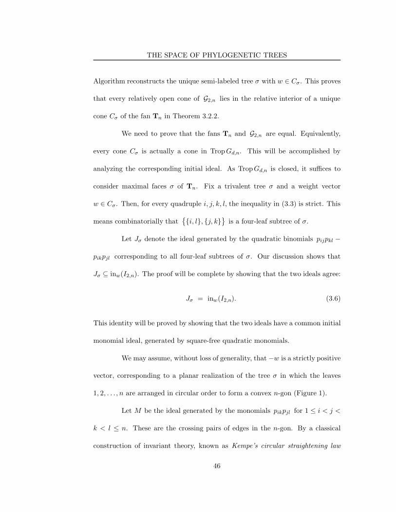
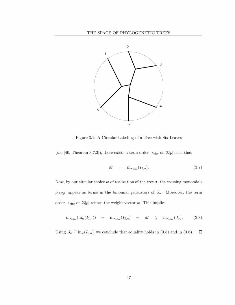
We may assume, without loss of generality, that −w is a strictly positive
vector, corresponding to a planar realization of the tree σ in which the leaves
1, 2, . . . , n are arranged in circular order to form a convex n-gon (Figure 1).
Let M be the ideal generated by the monomials pikpjl for 1 ≤ i < j <
k < l ≤ n. These are the crossing pairs of edges in the n-gon. By a classical
construction of invariant theory, known as Kempe’s circular straightening law
46
THE SPACE OF PHYLOGENETIC TREES
6
5
4
3
2
1
Figure 3.1: A Circular Labeling of a Tree with Six Leaves
(see [40, Theorem 3.7.3]), there exists a term order ≺circ on Z[p] such that
M = in≺circ(I2,n). (3.7)
Now, by our circular choice w of realization of the tree σ, the crossing monomials
pikpjl appear as terms in the binomial generators of Jσ . Moreover, the term
order ≺circ on Z[p] refines the weight vector w. This implies
in≺circ(inw(I2,n)) = in≺circ(I2,n) = M ⊆ in≺circ(Jσ). (3.8)
Using Jσ ⊆ inw(I2,n) we conclude that equality holds in (3.8) and in (3.6).
47
THE GRASSMANNIAN OF 3-PLANES IN 6-SPACE
3.3 The Grassmannian of 3-planes in 6-space
In this section we study the case d = 3 and n = 6. The Plucker ideal I3,6 is
minimally generated by 35 quadrics in the polynomial ring in 20 variables,
Z[p] = Z[p123, p124, . . . , p456].
We are interested in the 10-dimensional fan G3,6 which consists of all vectors
w ∈ R20 such that inw(I3,6) is monomial-free. The four-dimensional quotient
fan G ′′3,6 sits in R20/image(φ) ' R14 and is a cone over the three-dimensional
polyhedral complex G ′′′3,6. Our aim is to prove Theorem 3.1.6, which states that
G ′′′3,6 consists of 65 vertices, 535 edges, 1350 triangles, 990 tetrahedra and 15
bipyramids.
We begin by listing the vertices. Let E denote the set of 20 standard
basis vectors Eijk in R(63). For each 4-element subset i, j, k, l of 1, 2, . . . , 6 we
set
Fijkl = Eijk + Eijl + Eikl + Ejkl.
Let F denote the set of these 15 vectors. Finally consider any of the 15 triparti-
tions i1, i2, i3, i4, i5, i6 of 1, 2, . . . , 6 and define the vectors
Gi1i2i3i4i5i6 := Fi1i2i3i4 + Ei3i4i5 + Ei3i4i6
and Gi1i2i5i6i3i4 := Fi1i2i5i6 + Ei3i5i6 + Ei4i5i6 .
This gives us another set G of 30 vectors. All 65 vectors in E ∪ F ∪ G are
48

THE GRASSMANNIAN OF 3-PLANES IN 6-SPACE
regarded as elements of the quotient space R(63)/image(φ) ' R14. Note that
Gi1i2i3i4i5i6 = Gi3i4i5i6i1i2 = Gi5i6i1i2i3i4 .
Later on, the following identity will turn out to be important in the proof of
Theorem 3.3.4:
Gi1i2i3i4i5i6 + Gi1i2i5i6i3i4 = Fi1i2i3i4 + Fi1i2i5i6 + Fi3i4i5i6 . (3.9)
Lemma 3.3.1 and other results in this section were found by computation.
Lemma 3.3.1. The set of vertices of G3,6 equals E ∪ F ∪ G.
We next describe all the 550 edges of the tropical Grassmannian G3,6.
(EE) There are 90 edges like E123, E145 and 10 edges like E123, E456, for a
total of 100 edges connecting pairs of vertices both of which are in E. (By
the word “like”, we will always mean “in the S6 orbit of, where S6 permutes
the indices 1, 2, . . .6.”)
(FF) This class consists of 45 edges like F1234, F1256.
(GG) Each of the 15 tripartitions gives exactly one edge, like G123456, G125634.
(EF) There are 60 edges like E123, F1234 and 60 edges like E123, F1456, for
a total of 120 edges connecting a vertex in E to a vertex in F .
(EG) This class consists of 180 edges like E123, G123456. The intersections of
the index triple of the E vertex with the three index pairs of the G vertex
must have cardinalities (2, 1, 0) in this cyclic order.
49
THE GRASSMANNIAN OF 3-PLANES IN 6-SPACE
(FG) This class consists of 90 edges like F1234, G123456.
Lemma 3.3.2. The 1-skeleton of G ′′′3,6 is the graph with the 550 edges above.
Let ∆ denote the flag complex specified by the graph in the previous
lemma. Thus ∆ is the simplicial complex on E ∪ F ∪G whose faces are subsets
σ with the property that each 2-element subset of σ is one of the 550 edges. We
will see that G3,6 is a subcomplex homotopy equivalent to ∆.
Lemma 3.3.3. The flag complex ∆ has 1, 410 triangles, 1, 065 tetrahedra, 15
four-dimensional simplices, and it has no faces of dimension five or more.
The facets of ∆ are grouped into seven symmetry classes:
Facet FFFGG: There are 15 four-dimensional simplices, one for each partition
of 1, . . . , 6 into three pairs. The tripartition 1, 2, 3, 4, 5, 6. gives the
facet F1234, F1256, F3456, G123456, G125634; the other 14 cases can be determined
by the S6 symmetry. The 75 tetrahedra contained in these 15 four-simplices are
not facets of ∆.
The remaining 990 tetrahedra in ∆ are facets and they come in six
classes:
Facet EEEE: There are 30 tetrahedra like E123, E145, E246, E356.
Facet EEFF1: There are 90 tetrahedra like E123, E456, F1234, F3456.
Facet EEFF2: There are 90 tetrahedra like E125, E345, F3456, F1256.
Facet EFFG: There are 180 tetrahedra like E345, F1256, F3456, G123456.
50

THE GRASSMANNIAN OF 3-PLANES IN 6-SPACE
Facet EEEG: There are 240 tetrahedra like E126, E134, E356, G125634.
Facet EEFG: There are 360 tetrahedra like E234, E125, F1256, G125634.
While ∆ is an abstract simplicial complex on the vertices of G ′′′3,6, it
is not embedded as a simplicial complex because relation (3.9) shows that the
five vertices of the four dimensional simplices only span three dimensional space.
Specifically, they form a bipyramid with the F-vertices as the base and the G-
vertices as the two cone points.
We now modify the flag complex ∆ to a new polyhedral complex ∆′
which has pure dimension three and reflects the situation described in the last
paragraph. The complex ∆′ is obtained from ∆ by removing the 15 FFF-
triangles F1234, F1256, F3456, along with the 30 tetrahedra FFFG and the 15
four-dimensional facets FFFGG containing the FFF-triangles. In the place of
each four dimensional simplex, we instead put a bipyramid. We will give another
way of understanding the seven types of facets and three types of rays in Section
4.3.
The following theorem implies Theorem 3.1.6.
Theorem 3.3.4. The tropical Grassmannian G ′′′3,6 equals the polyhedral complex
∆′. It is not a flag complex because of the 15 missing FFF-triangles. The homol-
ogy of G ′′′3,6 is concentrated in (top) dimension 3; H3(G
′′′3,6,Z) = Z126.
The integral homology groups were computed independently by Michael
Joswig and Volkmar Welker. We are grateful for their help.
51
THE GRASSMANNIAN OF 3-PLANES IN 6-SPACE
This theorem is proved by an explicit computation. The correctness
of the result can be verified by the following method. One first checks that the
seven types of cones described above are indeed Grobner cones of I3,6 whose
initial ideals are monomial-free. Next one checks that the list is complete. This
relies on a result that will appear in a forthcoming paper which guarantees that
G3,6 is connected in codimension 1. The completeness check is done by computing
the link of each of the known classes of triangles. Algebraically, this amounts to
computing the (truly zero-dimensional) tropical variety of inw(I3,6) where w is
any point in the relative interior of the triangular cone in question. For all but
one class of triangles the link consists of three points, and each neighboring 3-cell
is found to be already among our seven classes. The links of the triangles are as
follows:
Triangle EEE: The link of E146, E256, E345 consists of E123, G163425, G142635.
Triangle EEF: The link of E256, E346, F1346 consists of F1256, G132546, G142536.
Triangle EEG: The link of E156, E236, G142356 consists of E124, E134, F1456.
Triangle EFF: The link of E135, F1345, F2346 consists of E236, E246, G153426.
Triangle EFG: The link of E235, F2356, G143526 consists of E145, F1246, E134.
Triangle FGG: The link of F1456, G142356, G145623 consists of F2356 and F1234.
52
Chapter 4
Tropical Linear Spaces
4.1 Introduction and Summary
In the preceding section we have described our attempts to study the tropical-
ization of the Grassmannian. Classically, the Grassmannian parameterizes linear
spaces of dimension d in n space. A similar statement is true of the Tropical
Grassmannian, namely:
Theorem 4.1.1. There is a bijection between the points of TropG(d, n) and the
collection of polyhedral complexes occurring as TropL for L a d-plane in Kn.
Just as it is best to study all matroids and then consider the realizable
matroids as a special subset among them, it turns out to be best to enhance the
notion of “TropL for L a d-plane in Kn” to a larger collection of combinatorial
objects which we will term tropical linear spaces. After we have investigated
53
INTRODUCTION AND SUMMARY
tropical linear spaces from a combinatorial perspective, we then turn in Section
4.5 to the question of identifying which such spaces occur as TropL. The reader
who prefers combinatorics to algebraic geometry may find this chapter a pleasant
break, as most of our arguments will be purely combinatorial.
Tropical linear spaces will be polyhedral complexes. Thus, we can ask
about all of the invariants associated to polyhedral complexes. Ardila and Klivans
[1] have studied the link of a vertex in a tropical linear space and have shown it to
be homeomorphic to the chain complex of the lattice of flats of a certain matroid
and thus, ([50], sect. 7.6), homotopic to a wedge of spheres. The polytopes
occurring in tropical linear spaces are Minkowski summands of permutahedra
(Proposition 4.2.5). The topology of tropical linear spaces is quite simple: they
are contractible (Theorem 4.2.8). So we understand the local combinatorics and
the local and global topology of tropical linear spaces.
The global combinatorics of tropical linear spaces, on the other hand,
is quite intriguing. There is a great deal of theoretical and some experimental
evidence for the following:
The f-Vector Conjecture. The number of i-dimensional faces of a tropical
d-plane in n-space which become bounded after being mapped to Rn/(1, . . . , 1)
is at most(
n−2id−i
)(
n−i−1i−1
)
.
Remark: It would follow from the f -vector conjecture that the num-
ber of total i-dimensional faces of a tropical d-plane in n-space, without any
54
INTRODUCTION AND SUMMARY
boundedness condition, is at most(n−i−1
d−i
)(2n−d−1i−1
)
. See Proposition 4.2.10.
The following is a summary of the rest of the chapter.
In Section 4.2, we will define the basic concepts mentioned in this intro-
duction and prove their essential properties. We will also introduce an operation
called dualization, which is analogous to the classical operation of taking the
dual, or orthogonal complement, of a linear space.
In Section 4.4, we will introduce an operation of transverse intersection
that produces new tropical linear spaces from old. We define a tropical linear
space to be constructible if it can be built from tropical hyperplanes (equivalently,
from points) by successive dualization and transverse intersection. Much of the
rest of the chapter will be devoted toward proving:
Theorem 4.1.2. Every constructible space achieves the f -vector of the f -vector
conjecture.
In Section 4.5, we discuss which tropical linear spaces are of the form
TropL for a linear space L or, as we will term it there, which are realizable. These
section includes many counter-examples to show that tropical linear spaces can
fail to be realizable in almost every conceivable way.
In Section 4.6 we will define a notion of “series-parallel tropical linear
space”, analogous to the notion of series-parallel matroid. We also describe a way
of working with series-parallel matroids in terms of two-colored trees that will be
important in the future. One of our themes will be that series-parallel tropical
55
INTRODUCTION AND SUMMARY
linear spaces are the best tropical linear spaces. In particular we conjecture
The f-Vector Conjecture, Continued. Equality in the f -vector conjecture
is achieved precisely by series-parallel linear spaces.
We will show that the tropical linear spaces which are easy to write
down are series parallel. More precisely,
Theorem 4.1.3. Every constructible space is series-parallel.
One unfortunate consequence of Theorem 4.1.3 is that it is quite hard
to find a general method for writing down tropical linear spaces that are not
series-parallel! More precisely, it is not so hard to produce degenerate limits
of series-parallel linear spaces which are not themselves series-parallel. Writing
down a large number of tropical linear spaces which are not limits of series-parallel
tropical linear spaces, however, is a challenge – which is one of the reasons that
experimentally testing the f -vector conjecture is tricky.
In Section 4.7, we will prove the f -vector conjecture in the cases i = 1
and d = bn/2c. We then return to proving our main results. We prove Theorem
4.1.3 in Section 4.8 and also prove many lemmas that will be used in the proof
of Theorem 4.1.2. We also prove Theorem 4.1.2 in Section 4.8.
Finally, in Section 4.9, we will introduce a notion of tree linear space
which achieves the bounds in the f -vector conjecture and has very explicit com-
binatorics. Suggestively, the construction of tree linear spaces will be reminiscent
of the construction of cyclic polytopes.
56
BASIC DEFINITIONS AND RESULTS
4.2 Basic Definitions and Results
We will adopt the convention of writing Trop(f) to mean the tropicalization of
the hypersurface generated by f .
Consider a collection of variables pi1...id indexed by the d element subsets
of [n] := 1, . . . , n. We will say that p is a tropical Plucker vector if
(pI) ∈ Trop(PSijPSkl − PSikPSjl + PSilPSjk)
for every S ∈( [n]d−2
)
and every i, j, k and l distinct members of [n] \ S.
Remark: This definition is equivalent to saying that pI is a valuated
matroid with values in the semiring (R,+,min). See [13] as well as the more
general [12] and [14].
Let ∆(d, n) denote the (d, n)-hypersimplex, defined as the convex hull
of the points ei1 + · · ·+eid ∈ Rn where i1, . . . , id runs over([n]
d
)
. We abbreviate
ei1 + · · · + eid by ei1 ...id . Consider a real-valued function i1, . . . , id 7→ pi1...id
on the vertices of ∆(d, n). We define a polyhedral subdivision Dp of ∆(d, n) as
follows: consider the points (ei1 + · · ·+ eid , pi1···id) ∈ ∆(d, n)× R and take their
convex hull. Take the lower faces (those whose outward normal vector have last
component negative) and project them back down to ∆(d, n), this gives us the
subdivision Dp. We will often omit the subscript p when it is clear from context.
A subdivision which is obtained in this manner is called regular, see, for example,
[51] definition 5.3.
Let P be a subpolytope of ∆(d, n). We say that P is matroidal if the
57
BASIC DEFINITIONS AND RESULTS
vertices of P , considered as elements of([n]
d
)
, are the bases of a matroid M . In
this case, we write P = PM . Our references for matroid terminology and theory
are Neil White’s anthologies [49] and [50].
Proposition 4.2.1. The following are equivalent:
1. pi1...id are tropical Plucker coordinates
2. The one skeleta of D and ∆(d, n) are the same.
3. Every face of D is matroidal.
Proof. (1) =⇒ (2). Every edge of D joins two vertices of ∆(d, n). If e is an
edge of D connecting eI and eJ , we define the length of e, denoted `(e), to be
|I \ J | = |J \ I |. Our claim is that every edge of e has length 1. We prove by
induction on ` ≥ 2 that D has no edge of length `.
For the base case, if e is an edge with `(e) = 2 then e = (eSij , eSkl) for
some S ∈(
[n]d−2
)
. The six vertices eSij , eSik , eSil, eSjk , eSjl, eSkl form the vertices
of an octahedron O with eSij and eSkl opposite vertices. One can check that the
condition (pI) ∈ Trop(PSijPSkl − PSikPSjl + PSilPSjk) implies that O is either a
face of D or subdivided in D into two square pyramids (in one of three possible
ways). In any of these cases, e is not an edge of D.
Now consider the case where ` > 2. Suppose (for contradiction) that e
is an edge of D. Let e = (eST , eST ′) with T ∩ T ′ = ∅ and |T | = |T ′| = `. Let F
be the face of ∆(d, n) consisting of all vertices eI with S ⊂ I ⊂ S ∪T ∪T ′. Then
58
BASIC DEFINITIONS AND RESULTS
e must belong to some two dimensional face of D contained in F ; call this two
dimensional face G.
Let γ be the path from eST to eST ′ that goes around G the other way
from e. No two vertices of F are more than distance ` apart, so the edges of γ
have lengths less than or equal to `. If γ contained an edge (eSU , eSU ′) of length
` then its midpoint (eSU + eSU ′)/2 would also be the midpoint of e contradicting
the convexity of G. Thus, every edge of γ has length less than ` and by induction
must have length 1. So all the edges of γ are in the direction ei − ej for some
i and j ∈ [n]. These vectors must span a two dimensional space. This means
either that there are i1, i2, j1, j2 ⊂ [n] such that all edges of γ are parallel to
some eir − ejs or there are i1, i2, i3 ⊂ [n] such that every edge of γ is parallel
to eir − eis . In either case, e has length at most 2, but that returns us to our
ground case.
(2) =⇒ (3): Let P be any polytope in D. By assumption, all of the
edges of P are edges of ∆(d, n). It is a theorem of Gelfand, Goresky, MacPherson
and Serganova ([20], theorem 4.1) that this implies that P is matroidal. Since
the proof is short, we include it. Let eI and eJ be vertices of P with j ∈ J \ I .
We must prove that there is a vertex of P of the form eI∪j\b for some b ∈ I .
Define a linear functional φ : ∆(d, n) → R by φ(x1, . . . , xn) =∑
i∈I xi +
dxj . Then Q := P ∩ x : φ(x) ≥ d is a convex polytope and hence connected.
Q contains the vertices eI and eJ and there is a path from eI to eJ along edges
59
BASIC DEFINITIONS AND RESULTS
of P which lie in Q. Let the first step of this path go from eI to eI∪a\b. If
a 6= j then φ(eI∪a\b) = d− 1 and eI∪a\b does not lie in Q. So instead we
have a = j and we are done.
(3) =⇒ (1): It is easy to check that, if (1) is false, D has a one
dimensional face of the form Hull(eSij , eSkl), with i, j, k and l distinct. This is
not matroidal.
Now, suppose that (pI) ∈ R([n]d ) obeys the tropical Plucker relations.
Define L(p) ⊂ Rn by
⋂
1≤j1<···<jd+1≤n
Trop(
d+1∑
r=1
(−1)rPj1···jr ···jd+1Xjr).
We term any L which arises in this manner a d-dimensional tropical linear space
in n-space. We often omit the dependence on p when it is clear from context.
L(p) is essentially the same set as the tight span of p defined in [15].
There are two differences: (1) Dress’s sign conventions are opposite to ours and
(2) L(p) is invariant under translation by (1, . . . , 1); Dress chooses a particular
representative within each orbit for this translation.
While the above definition makes the connection to ordinary linear
spaces most clear, for practically every purpose it is better to work with the
alternate characterization which we now give. For any w ∈ Rn, define Dw to be
the subset of the vertices of ∆(d, n) at which pi1...id −∑d
j=1 wij is minimal. This
is, by definition, a face of D and thus is PMw for a matroid Mw.
Proposition 4.2.2. w ∈ L(p) if and only if Mw is loop-free.
60
BASIC DEFINITIONS AND RESULTS
Recall that a matroid is called loop-free if every element of the matroid
appears in at least one basis. There is a geometric way of recognizing when M is
loop-free from the polytope PM : M is loop-free if and only if PM is not contained
in any of the n facets of ∆(d, n) of the type xi = 0 for 1 ≤ i ≤ n. In particular,
note that if PM meets the interior of ∆(d, n) then M is necessarily loop-free.
Proof. By replacing pi1...id by pi1...id −∑d
j=1 wij − (constant), we may assume
without loss of generality that w = 0 and min pI = 0. Then Mw = M0 is simply
the matroid whose basis correspond to the I for which pI = 0. First, we assume
that M0 has a loop j and prove that 0 6∈ L(p). Let (i1, . . . , id) be a basis of M0,
clearly j 6∈ (i1, . . . , id). Then pi1...id = 0 but pji1 ...ir ...id> 0 for 1 ≤ r ≤ d. Taking
(j1, . . . , jd+1) = (j, i1, . . . , id) we see that 0 6∈ Trop(∑d+1
r=1(−1)rPj1...jr ...jd+1Xjr).
The converse is more interesting. Fix J = j1, . . . , jd+1, our aim will
be to prove 0 ∈ Trop(∑d+1
r=1(−1)rPj1 ...jr ...jd+1Xjr). Let eJ =
∑
ejr and, for any
s ∈ R, set Ms = M−seJ. Note that, for s large enough, all of the bases of Ms
will be subsets of J . It is equivalent to show that, for such an s, the matroid Ms
has at least two bases. In other words, we must show that for any j ∈ J and
any such s, j is not a loop of Ms. By hypothesis, j is not a loop of M0, so it is
enough to show that if j ∈ J is a loop of Ms for some s then it is a loop of Ms′
for all s′ < s.
As s varies, Ms changes at a finite number of values of s, call them
s1 < s2 < · · · < sk . Suppose that si < s < si+1, then PMs is a face of both PMsi
61

BASIC DEFINITIONS AND RESULTS
and of PMsi+1. The bases of Ms are precisely the bases of Msi
which have the
largest possible number of elements in common with J . Similarly, the bases of
Ms are precisely the bases of Msi+1 which have the smallest possible number of
elements in common with J . In other words,
Ms = Msi|J ⊕Msi
/J = Msi+1 |[n]\J ⊕Msi+1/([n] \ J).
From the displayed equation, it follows that if j ∈ J is a loop in Msi+1
then it is a loop in Ms. Similarly, if j is a loop in Ms then it is a loop in Msi.
Concatenating deductions of this sort, we see that, as promised, if j is a loop of
Ms then it is a loop of Ms′ for all s′ < s.
As ∆(d, n) is contained in the hyperplane x1 + · · ·+ xn = d we see that
L is invariant under translation by (1, 1, . . . , 1). We will abuse notation by saying
a face of L is bounded if its image in Rn/(1, . . . , 1) is bounded and calling a face
a vertex if its image in Rn/(1, . . . , 1) is zero dimensional. However, when we refer
to the dimensions of faces of L we will always be speaking of L itself, without
taking the quotient by (1, . . . , 1).
We see that L is a subcomplex of D∨, where D∨ is defined to be the
polyhedral subdivision of Rn where w and w′ lie in the same face if Mw = Mw′ .
In Figure 4.1, we show ∆(2, 4), which is an octahedron, subdivided into two
square pyramids and draw the dual L/(1, 1, 1, 1) in bold. Notice that four of the
triangular faces of the octahedron correspond to a loop-free matroid consisting
of two parallelism classes, of sizes 1 and 3, while the other four faces correspond
62

BASIC DEFINITIONS AND RESULTS
Figure 4.1: A Subdivision of ∆(2, 4) and the Corresponding L/(1, 1, 1, 1)
to the matroid consisting of a single loop and no other relations. We write M∨
for the face of D∨ dual to PM . If v = M∨/(1, . . . , 1) is a vertex of L/(1, . . . , 1)
we see that the link of L/(1, . . . , 1) at v is the subcomplex of the normal fan to
PM consisting of the normals to the loop-free facets. This fan is studied in [1],
we summarize the main results of that paper in the following proposition:
Proposition 4.2.3. linkM∨(L) is homeomorphic to the chain complex of the
lattice of flats of L. If N∨ is a face of L containing v then N =⊕
Qk+1/Qk for
some flag of flats ∅ = Q0 ⊂ Q1 ⊂ · · · ⊂ Qr = [n] of M . The local cone of N
at M is given by those vectors which are constant on the set Qk \Qk−1 and for
which X(Qk \Qk−1) > X(Qk−1 \Qk−2)
When M∨/(1, . . . , 1) is positive dimensional, PM turns out to be a prod-
uct of PN ’s.
63
BASIC DEFINITIONS AND RESULTS
Proposition 4.2.4. Let M be a matroid with M =⊕
Mi the decomposition of
M into connected parts. Then PM =∏
PMi.
Proof. By the definition of direct sum, the bases of M are all combinations of
bases of the Mi.
We can now describe the faces of L. Recall that the braid arrangement
Br is the fan in Rr whose facets are the cones of the type xσ(1) ≤ . . . ≤ xσ(r)
where σ ranges over the symmetric group Sr.
Proposition 4.2.5. If M∨ is an r-dimensional face of L then the normal fan to
M∨ is a subfan of a coarsening of Br. When M∨ is bounded, M∨ is a Minkowski
summand of the rth permutahedron.
Proof. The normal fan to M∨ is the same as the link of PM in D. Let PM be
a face of D with PM a face of PM . We must show that the local cone of PM at
PM is a union of cones of Br. But the local cone of PM at PM is precisely the
negative of the cone of the normal fan to PM dual to PM . From the description
in [1], we see that the normal fan to PM is a coarsening of Bn and that the cones
dual to codimension i faces are unions of cones of Br.
If M∨ is bounded then its normal fan is complete and thus, by the last
paragraph, a coarsening of Br. Br is the normal fan to the rth permutahedron.
If P and Q are two polytopes such that the normal fan to Q refines that of P
then P is a Minkowski summand of tQ for t sufficiently large.
64
BASIC DEFINITIONS AND RESULTS
Not every coarsening of Br is the normal fan to a polytope. For example,
take a cube, divide one of its faces into two triangles and cone from the center.
This is a coarsening of B4 which is not the normal fan of any polytope. I do not
know whether there are further obstructions to a fan showing up as the normal
fan to a face of a tropical linear space.
Problem 4.2.6. Let P be a polytope whose normal fan is a coarsening of Br.
Can P always occur as a face of a tropical linear space?
For ordinary linear spaces, the linear space determines the Plucker co-
ordinates up to scaling. For tropical linear spaces, a similar result holds.
Proposition 4.2.7. Let L be a tropical linear space with tropical Plucker coor-
dinates pI . Then L determines the pI up to addition of a common scalar.
Proof. Let S be a d−1 element subset of [n] and let F denote the face of ∆(d, n)
whose vertices are those I containing S. Since F is an (n − d)-simplex, it can
not be subdivided in D so F is a face of D. F corresponds to a loop-free matroid
Φ so it is dual to a face Φ∨ of L. Φ∨ is of the form (RS≥0 + R(1, . . . , 1)) + q
for q a vector satisfying qi = pSi for i 6∈ S. No other face of L is of the form
(RS≥0 ⊕ R(1, . . . , 1)) + q and q is unique up to translation by (1, . . . , 1). Thus, L
determines pSi − pSj . As this is true for all S, i and j, we see that L determines
the pI up to adding the same constant to all of them.
Theorem 4.2.8. L is a pure d-dimensional contractible polyhedral complex.
65
BASIC DEFINITIONS AND RESULTS
Proof. To show that L is pure d-dimensional, it is enough to show that the
link of any vertex v of L/(1, . . . , 1) is a pure (d − 2)-dimensional complex. Let
v + (1, . . . , 1) be dual to PM for some matroid M . By the results of [1], the link
of v has a subdivision isomorphic to the order complex of the lattice of flats of
M . This lattice is graded of length d, so its order complex is pure of dimension
d− 2.
We now show contractibility. It is easy to see that each tropical hyper-
plane is tropically convex in the sense of [11]. Thus, their intersection is tropically
convex and hence contractible.
We now study the bounded faces of L.
Proposition 4.2.9. The following are equivalent:
1. w lies in a bounded face of L
2. PMw is an interior face of D.
3. Mw is loop-free and co-loop-free.
Proof. (2) ⇐⇒ (3): PMw is interior if and only if it is not contained in any facet
of ∆(d, n). The facets of ∆(d, n) are of two types: xi = 1 and xi = 0. PMw lies
in the former type if and only if i is a co-loop of Mw; PMw lies in the latter type
if and only if i is a loop of Mw .
(1) ⇐⇒ (2): If P is not an interior face of D, the corresponding dual
face is not bounded. Conversely, if P is internal, the corresponding dual face of
66
BASIC DEFINITIONS AND RESULTS
D∨ is bounded, so we just must check that this dual face is in L(p) at all. For
this, we must check that Mw is loop-free. But we saw in the previous paragraph
that this follows from PMw being internal.
At this point, we can prove our earlier remark.
Proposition 4.2.10. If the f -vector conjecture is true then a tropical d-plane
in n-space has no more than(
n−i−1d−i
)(
2n−d−1i−1
)
faces of dimension i.
Proof. Let D be a matroidal decomposition of ∆(d, n). We must bound the
number of codimension i− 1 faces PM of D such that M has no loops. For such
a PM , let Λ ⊂ [n] be the co-loops of M and let ∆ be the face of ∆(d, n) whose
vertices are the sets I ∈([n]
d
)
which contain Λ. The claim that M has no loops
is equivalent to saying that PM is an interior face of the decomposition of ∆. So
we may count the total number of PM by summing over all such faces ∆.
There are(n
j
)
faces ∆ for which |Λ| = j; each such ∆ is isomorphic to
∆(d−j, n−j). A subpolytope of such a ∆ has codimension i−1 in ∆(d, n) if and
only if it has co-dimension i− j − 1 in ∆. So, assuming the f -vector conjecture
and writing the bound in the f -vector conjecture as(
n−i−1d−i
)(
n−d−1i−1
)
, we have the
following bound for the number of co-dimension i− 1 loop-free faces of D:
67
BASIC DEFINITIONS AND RESULTS
∑
j
(
n
j
)(
(n− j)− (i− j)− 1
(d− j)− (i− j)
)(
(n− j)− (d− j)− 1
(i− j) − 1
)
=
(
n− i− 1
d− i
)
∑
j
(
n
j
)(
n − d− 1
i− j − 1
)
=
(
n − i− 1
d− i
)(
2n− d− 1
i− 1
)
.
The last sum is evaluated by the identity∑
j
(
pj
)(
qr−j
)
=(
p+qr
)
.
Suppose that p :([n]
d
)
→ R obey the tropical Plucker relations. Define
p⊥ :( [n]n−d
)
→ R by p⊥I = p[n]\I . Then the subdivision D⊥ of ∆(n− d, n) induced
by p⊥ is simply the image of D under (x1, . . . , xn) 7→ (1 − x1, . . . , 1 − xn). This
map replaces each matroidal polytope with the polytope of the dual matroid; in
particular, p⊥ also obeys the tropical Plucker relations. We denote L(p⊥) by L⊥.
We can easily check that L 7→ L⊥ is an inclusion reversing bijection from the set
of tropical linear spaces in Rn to itself.
We will use this dualization operation to defien a large class of con-
structible tropical linear spaces, which are built out of repeated simple opera-
tions. It is also useful for discussing questions such as whether a given tropical
linear space is an intersection of a given number of tropical hyperplanes, as the
dual version of this questions is often easier to visualize.
Proposition 4.2.11. The bounded part of L⊥ is negative that of L. If L is a
tropical linear space of dimension d in n space then the bounded part of L is at
most min(d, n− d)-dimensional.
68
TropG(3, 6) AND MATROIDAL DECOMPOSITIONS
Proof. The first sentence follows because the property of being loop- and co-
loop-free is self dual. L is d-dimensional and L⊥ is (n − d)-dimensional; as
the bounded part of L is isomorphic to a subcomplex of both it is at most
min(d, n− d)-dimensional.
4.3 Trop G(3, 6) and Matroidal Decompositions
Now that we have the terminology of matroidal subdivisions available to us, it is
worthwhile to see how it can be used to described the various faces of TropG(3, 6)
in Section 3.3. There are three types of rays of TropG(3, 6), which we referred
to as types E, F and G. Each of these correspond to a minimal decomposition
of ∆(3, 6) into matroidal polytopes.
The ray Eijk corresponds to a subdivision of ∆(3, 6) into two polytopes:
the first is the convex hull of the vertex eijk and all of its neighbors (as a polytope,
this is isomorphic to the cone on the product of two triangles) and the second is
the convex hull of all vertices except for eijk. As matroids, these two polytopes
correspond to the point configurations in Figure 4.2.
The ray Fijkl also corresponds to the splitting of ∆(3, 6) into two poly-
topes. One is the convex hull of all of the vertices eabc where |a, b, c∩i, j, k, l|
is either 2 or 3, the other is the convex hull of all vertices eabc where this inter-
section has size 1 or 2. These correspond to the dual matroid in Figure 4.3.
Finally, the rayGijklmn corresponds to the decomposition of ∆(3, 6) into
69
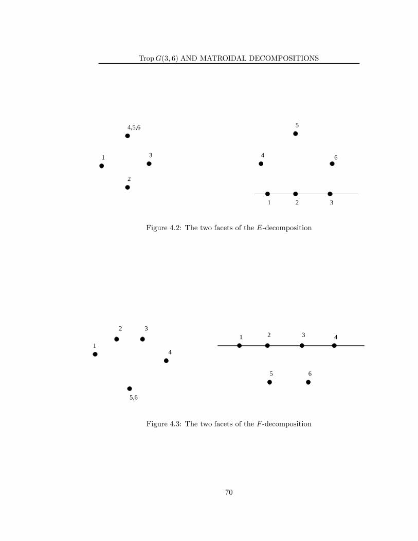
TropG(3, 6) AND MATROIDAL DECOMPOSITIONS
1 2 3
4
5
6
4,5,6
1
2
3
Figure 4.2: The two facets of the E-decomposition
5,6
1
2 3
4
1 2 3 4
5 6
Figure 4.3: The two facets of the F -decomposition
70
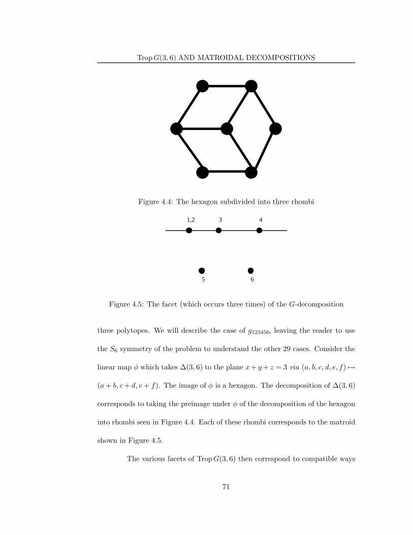
TropG(3, 6) AND MATROIDAL DECOMPOSITIONS
Figure 4.4: The hexagon subdivided into three rhombi
1,2 3 4
5 6
Figure 4.5: The facet (which occurs three times) of the G-decomposition
three polytopes. We will describe the case of g123456, leaving the reader to use
the S6 symmetry of the problem to understand the other 29 cases. Consider the
linear map φ which takes ∆(3, 6) to the plane x+ y+ z = 3 via (a, b, c, d, e, f) 7→
(a+ b, c+ d, e+ f). The image of φ is a hexagon. The decomposition of ∆(3, 6)
corresponds to taking the preimage under φ of the decomposition of the hexagon
into rhombi seen in Figure 4.4. Each of these rhombi corresponds to the matroid
shown in Figure 4.5.
The various facets of TropG(3, 6) then correspond to compatible ways
71
TropG(3, 6) AND MATROIDAL DECOMPOSITIONS
of superimposing these decompositions. The type FFFGG, for example, can be
described using the map φ of the previous paragraph as the decomposition of
the hexagon into six equilateral triangles. Each of the vertices of the bipyramid
corresponds to a different coarsening of this decomposition; see Figure 4.6. The
reader may enjoy labelling the other faces of the bipyramid with intermediate
decompositions of the hexagon.
It is possible to largely visualize the other facets of TropG(3, 6) as pull-
backs of decompositions of the hexagon as well. In each picture of Figure 4.7, we
show a hexagon broken up into triangles and rhombi and decorated with some
circular arcs. The meaning in each case is to pull back the decompositions into
triangles and rhombi along φ, thus obtaining a decomposition of ∆(3, 6). Then,
for each circled vertex of the hexagon, we take a vertex e of ∆(3, 6) that maps
to this circled vertex under φ. We then slice off e and all of its neighbors as a
seperate piece of the decomposition. In most cases, all choices of e are equivalent
up to S6 symmetry. The cases EEFF1 and EEFF2 are distinguished by the
fact that, in type EEFF1, the two circled vertices are lifted to antipodal points
of ∆(3, 6) and in type EEFF2 they are lifted to non-antipodal points. In type
EEEE, the four lifts must be chosen in the unique way (up to S6 symmetry) that
none of them are adjacent. The best way to describe this is that the remaining
central region after these 4 vertices have been sliced off must correspond to the
graphical matroid of K4.
72
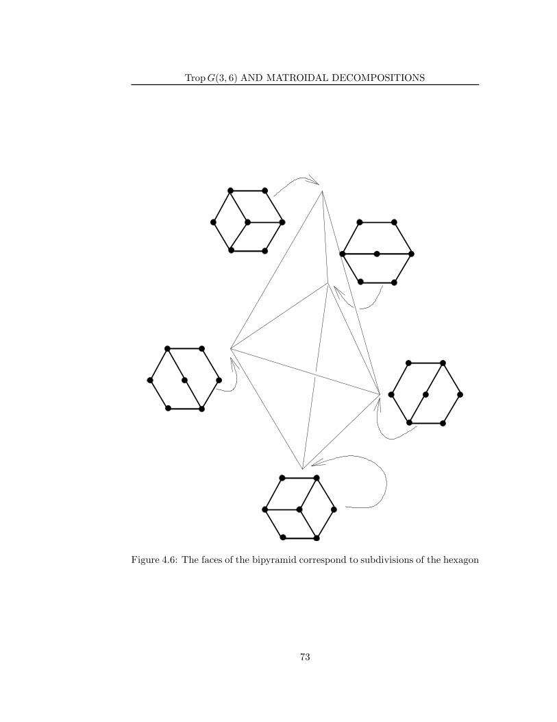
TropG(3, 6) AND MATROIDAL DECOMPOSITIONS
Figure 4.6: The faces of the bipyramid correspond to subdivisions of the hexagon
73
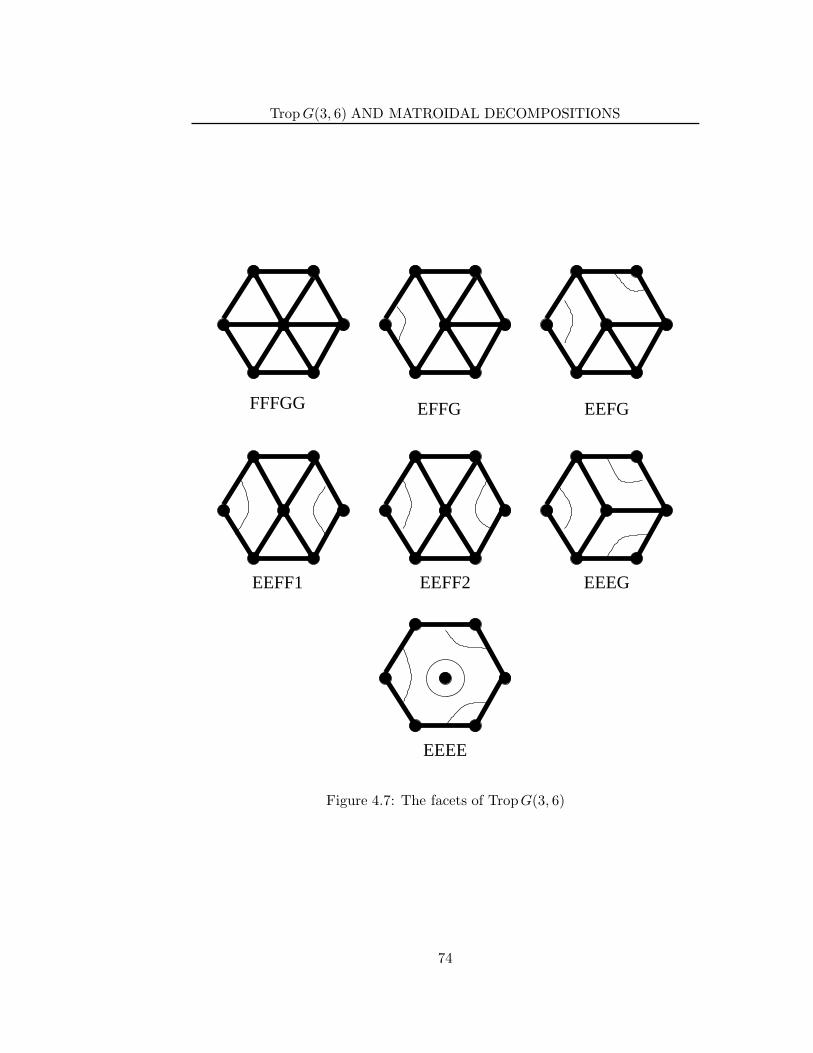
TropG(3, 6) AND MATROIDAL DECOMPOSITIONS
FFFGG EFFG EEFG
EEFF1 EEFF2 EEEG
EEEE
Figure 4.7: The facets of TropG(3, 6)
74
STABLE INTERSECTIONS
4.4 Stable Intersections
If L and L′ are two ordinary linear spaces of dimensions d and d′ in n space which
meet transversely then L ∩ L′ is a (d+ d′ − n)-dimensional space whose Plucker
coordinates are given by
PJ (L ∩ L′) =∑
I∩I ′=J|I |=d|I ′|=d′
±PI(L)PI ′(L′).
Note that the summation conditions on I and I ′ guarantee that I ∪ I ′ = [n].
We will discuss a tropical version of this formula. If L and L′ are tropical
linear spaces of dimension d and d′, define a real valued function p(L ∩stable
L′) on
( [n]d+d′−n
)
by
pJ(L ∩stable
L′) = minI∩I ′=J|I |=d|I ′|=d′
(pI(L) + pI ′(L′)).
At the moment, pJ(L ∩stable
L′) is just defined as a formal symbol, there
is not yet any tropical linear space called L ∩stable
L′. We now prove that there is
such a space.
Proposition 4.4.1. p(L ∩stable
L′) is a tropical Plucker vector.
Proof. Set P to be the polyhedron of points above the lower convex hull of the
points (pi1...id(L), ei1 + · · · + eid) ∈ R × ∆(d, n) and define P ′ ⊂ R × ∆(d′, n)
similarly. Include ∆(d + d′ − n, n) into the Minkowski sum ∆(d, n) + ∆(d′, n)
by ι : e 7→ e + (1, . . . , 1). Set Q = (P + P ′) ∩ (R × ι(∆(d + d′ − n, n))). Let
75
STABLE INTERSECTIONS
J ∈( [n]d+d′−n
)
. The height of Q above the vertex ι(eJ ) of ι(∆(d+ d′ − n, n) is
mineI∩eI′=ι(eJ )
|I |=d|I ′|=d′
pI + pI ′ = minI∩I ′=J|I |=d|I ′|=d′
pI + pI ′ .
So we see that projecting the bottom faces of Q back down to ∆(d + d′ − n, n)
yields the regular subdivision of ∆(d+ d′ − n, n) induced by p(L ∩stable
L′).
So we see that every face of Dp(L ∩stable
L′) is of the form
R := ι(∆(d+ d′ − n, n))∩ (PM + PM ′) .
The vertices of this face are the points ι(eJ) ∈ ι(∆(d+d′−n, n)) where J = I∩I ′
for I and I ′ bases of M and M ′ with I ∪ I ′ = [n].
There is an operation M ∧M ′, called matroid intersection ([49], section
7.6), which takes two matroids of ranks d and d′ and produces a third matroid.
The spanning sets of M ∧M ′ are precisely the sets of the form U ∩ U ′ where U
and U ′ span M and M ′ respectively. M ∧M ′ always has rank at least d+d′−n.
If the rank of M ∧M ′ is larger than d+ d′ − n then there are no pairs of bases
I and I ′ of M and M ′ with I ∪ I ′ = [n]. In this case R is empty and does not
contribute a face to Dp(L ∩stable
L′). Alternatively, the rank of M ∧M ′ is d+ d′ − n.
Then we see that R = PM∧M ′.
We have the immediate corollary
Corollary 4.4.2. Every face of Dp(L ∩stable
L′) is of the form PM∧M ′ for PM and
PM ′ faces of Dp(L) and Dp(L′).
76
STABLE INTERSECTIONS
We thus see that there is a well defined tropical linear space L ∩stable
L′.
Our aim now is to justify the notation L ∩stable
L′ by showing that L ∩stable
L′ is the
“stable” intersection of L and L′. We first need a definition and a combinatorial
lemma:
Let M and M ′ be two loop-free matroids on [n] with connected decom-
position M =⊕
i∈I Mi and M ′ =⊕
i∈I ′ M′i . Let Si and S ′
i be the ground sets of
Mi and M ′i . Let Γ(M,M ′) be the bipartite graph (possibly with multiple edges)
whose vertex set is ItI ′ and which has an edge between i and i′ for each element
of Si ∩S′i′ . We say that M and M ′ are transverse if Γ(M,M ′) is a forest without
multiple edges.
Lemma 4.4.3. Suppose that M and M ′ are transverse and let Γ = Γ(M,M ′).
Then M ∧M ′ is a loop-free matroid whose connected components are in bijection
with the components of Γ. M ∧M ′ is the matroid formed by repeatedly taking
parallel connections along the edges of Γ. M ∧M ′ has rank d+ d′ − n.
The phrase “repeatedly taking parallel connections” deserves a proper
definition, which will unfortunately be somewhat lengthy. What we mean is the
following: let F be a forest, let E be a finite set and let each edge of F be
labeled with an element of E, no two edges receiving the same label. Suppose
that, for each vertex v ∈ F , we are given a subset S(v) of E. We require that
S(v)∩S(w) = e if e is the edge (v, w), that S(v)∩S(w) = ∅ if there is no edge
joining v and w and that⋃
v∈F S(v) = E. For every v ∈ F , we place the structure
77
STABLE INTERSECTIONS
of a connected loop-free matroid M(v) on S(v). We then define a matroid N on
the ground set E by the following procedure:
1. If F has no edges, let N =⊕
v∈F M(v).
2. Otherwise, let v and w be vertices of F joined by an edge e.
3. Form a new forest F ′ where e is contracted to a single vertex u. Set
S ′(u) = S(v) ∪ S(w) and let M ′(u) be the parallel connection of M(v)
and M(w) along e. For all t ∈ F other than u, set S ′(t) = S(t) and
M ′(t) = M(t).
4. Return to step (1) with the new forest F ′ and the new S ′(·) and M ′(·).
The claim is that (a)N does not depend on the order of the contractions
and (b) N = M ∧M ′ when we take F = Γ, S(i) = S(′)i and M(i) = M
(′)i . Here
S(′)i is shorthand for “Si if i ∈ I and S ′
i if i ∈ I ′ and similarly for M(′)i .
Proof. Let T , S(·) and M(·) be as above and let N(F, S(·),M(·)) be the ma-
troid constructed by the above procedure. We claim that U ⊂ E is a basis of
N(F, S(·),M(·)) if and only if there exist bases B(v) of M(v) such that, for every
e ∈ E, precisely one of the following four conditions holds:
1. e ∈ U , e = (v, w) is an edge of F and e ∈ B(v) ∩B(w).
2. e ∈ U , e ∈ S(v) is not an edge of F and e ∈ B(v).
78
STABLE INTERSECTIONS
3. e 6∈ U , e = (v, w) is an edge of F and e lies in precisely one of B(v) and
B(w).
4. e 6∈ U , e ∈ S(v) is not an edge of F and e 6∈ B(v)
This is the definition of direct sum when F has no edges and it is easy to
check that this description is unchanged by contracting an edge, so this is indeed
a correct description of the bases of N(F, S(·),M(·)). Note that this description
is independent of the order of contractions, so we see that N(T, S(·),M(·)) is
independent of the order of contraction.
Applying the above description in the case where F = Γ(M,M ′) etc.,
we see that the bases of N(Γ,M(·), S(·)) are precisely the sets of the form B∩B′
where B and B′ are bases of M and M ′ with B∪B′ = [n]. If M and M ′ are such
that there exist bases B and B′ with B ∪B′ = [n] then the bases of M ∧M ′ are
exactly the sets of the form B∩B′ for such (B,B′). But the iterative construction
above clearly does produce a matroid and every matroid has at least one basis,
so such B and B′ do exist. |B ∩ B′| = |B| ∪ |B′| − |B ∪ B′| so N has rank
d+ d′ − n. Finally, observe that parallel connections preserves loop-freeness, so
N is loop-free.
Proposition 4.4.4. Let 0 ≤ d, d′ ≤ n with d+d′ ≥ n. Suppose that L and L′ are
tropical linear spaces in n-space of dimension d and d′. Then L ∩stable
L′ ⊆ L∩L′.
If L and L′ meet transversely then L ∩stable
L′ = L ∩ L′.
79
STABLE INTERSECTIONS
Proof. Let D, D′ and E be the subdivisions of ∆(d, n), ∆(d′, n) and ∆(d+d′−n, n)
corresponding to L, L′ and L ∩stable
L′. Let D∨, (D′)∨ and E∨ denote the dual
subdivisions of Rn.
Consider a particular w ∈ Rn, we need to show that w ∈ L ∩stable
L′
implies that w ∈ L and w ∈ L′ and that the reverse holds if L and L′ meet trans-
versely. Let M∨, (M ′)∨ and N∨ be the faces of D∨, (D′)∨ and E∨ respectively
containing w and let PM , PM ′ and PN be the respective dual faces of D, D′ and
E . Then PN = (PM + PM ′) ∩ ι(∆(d+ d′ − n, n)). We must show that, if M or
M ′ has a loop then N has a loop and that, if L and L′ meet transversely and N
has a loop then M or M ′ does as well.
First, suppose that M contains a loop e. Then, for every x ∈ PM , we
have xe = 0. For every x ∈ PM ′ we have xe ≤ 1. Thus, for x ∈ PM +PM ′ , xe ≤ 1
and thus xe = 0 on PN . So e is a loop of N .
Now assume that L and L′ meet transversely. Let M =⊕
i∈I Mi and
M ′ =⊕
i∈I ′ M′i be the components of M and M ′ and let Si and S ′
i be the ground
sets of Mi and M ′i respectively.
Lemma 4.4.5. M and M ′ are transverse, i.e., Γ(M,M ′) is a forest and has no
multiple edges.
Proof. Let |I | = e and |I ′| = e′, so e and e′ are the dimensions of M∨ and (M ′)∨.
The affine linear space spanned by M∨ is cut out by the equations xi − xj =
constant when edges i and j have the same endpoint in I , and similarly for
80
STABLE INTERSECTIONS
(M ′)∨. Thus, M∨ ∩ (M ′)∨ spans the affine linear space cut out by the equations
xi − xj = constant whenever edges i and j are in the same component of Γ.
We assumed that L and L′ meet transversely, so the dimension of the last linear
space must be e + e′ − n and Γ must have e + e′ − n connected components. A
graph with e+ e′ vertices, n edges and e+ e′−n connected components must be
a forest without multiple edges.
We now know by Lemma 4.4.3 that M ∧M ′ is loop-free.
The next theorem explains the motivation for the notation L ∩stable
L′
and the geometric meaning of L ∩stable
L′ when L and L′ are not transverse.
Theorem 4.4.6. Let L and L′ be tropical linear spaces. Then, for a generic v ∈
Rn, the linear spaces L and L′ + v meet transversely and L ∩stable
L′ = limv→0(L∩
(L′ + v)) where the limit is taken through generic v.
Proof. Let F and F ′ be faces of L and L′. Suppose that the affine linear spaces
spanned by F and F ′ together fail to span Rn. Then, for v outside a proper
subspace of Rn we have F ∩ (F ′ + v) = ∅. Thus, for a generically chosen v, every
such F and F ′ + v fail to meet. The only faces of L and L′ + v that do meet,
then, meet transversely.
We have pI(L′+v) = pI(L
′)+∑
i∈I vi so the tropical Plucker coordinates
of L′ + v vary continuously with v. The tropical Plucker coordinates of L ∩stable
(L′ + v) similarly vary continuously with v. When v is chosen generically, L and
81
REALIZABILITY OF TROPICAL LINEAR SPACES
L′ + v meet transversely so L ∩ (L′ + v) = L ∩stable
(L′ + v). Take limits of both
sides as v → 0 and use the proceeding continuity arguments to conclude that
limv→0(L∩ (L′ + v)) = L ∩stable
L′.
4.5 Realizability of Tropical Linear Spaces
In this section, we will discuss the question of which tropical linear spaces are
tropicalizations of actual linear spaces. In this section, we will denote actual
linear spaces (over K or κ) by boldface characters such as L.
Let L be a linear space with Plucker coordinates Pi1...id 6= 0. Let
pi1...id = v(Pi1...id). The P ’s obey the Plucker relations, so the p’s obey the
tropical Plucker relations. Our next proposition shows that the combinatorially
defined L(p) truly does reflect the geometrically defined Trop L.
Proposition 4.5.1. We have Trop L = L(p).
Proof. Every point (x1, . . . , xn) in L obeys∑
(−1)rPj1 ...bjr ...jd+1Xjr = 0 so the
v(Xi) lie in Trop(∑d+1
r=1(−1)rPj1 ···jr ···jd+1Xjr). Thus, Trop L ⊆ L(p).
For the converse direction, suppose w ∈ L(p), we will prove that w ∈
TropL. Without loss of generality, let w = 0 and suppose that 0 = minI∈([n]
d ) pI .
Let PI(0) ∈ κ be the image of PI in κ = R/M. Clearly, the PI (0) obey the
Plucker relations and hence correspond to an ideal L(0) ⊂ κn. It is easy to see
that L(0) = inw L. Let M be the set of I for which pI = 0. By assumption,
M is the set of bases of a loop free matroid. So L(0) is not contained in any
82
REALIZABILITY OF TROPICAL LINEAR SPACES
of the coordinate planes of κn and thus the corresponding ideal contains no
monomial.
We can now prove Theorem 4.1.1.
Theorem 4.5.2. The points of G ′d,n parameterize the possible subsets of Rn that
can occur as TropL for L a d-dimensional linear space in Kn with all Plucker
coordinates nonzero.
Proof. First, suppose that L is such a linear space with Plucker coordintes PI 6= 0.
Then TropL = L(v(P )), by the above proposition. By Proposition 4.2.7,L(v(P ))
determines v(P ) up to an additive constant. Thus, we see that TropL determines
a point of TropG(d, n)/(1, . . . , 1) = G ′d,n.
On the other hand, if p is a point of TropG(d, n) then pI = v(PI) for PI
the actual Plucker coordinates of some linear space L. Then L(p) is determined
by p and the above proposition shows that Trop L = L(p). So every point Gd.n
does give rise to a polyhedral complex in Rn of the form Trop L. The two maps
are easily seen to be inverse.
It also turns out that ∩stable
does actually capture the behavior of linear
spaces under intersection.
Proposition 4.5.3. Let L and L′ ⊂ Kn be two linear spaces. Then there exists
a linear space L′ ⊂ Kn with Trop L′ = TropL′ and TropL ∩
stable
Trop L′ =
TropL ∩stable
Trop L′ = Trop(L ∩ L′). If Trop L and TropL′ meet transversely,
83
REALIZABILITY OF TROPICAL LINEAR SPACES
then we already have TropL ∩stable
Trop L′ = Trop(L∩L
′) without having to choose
an L′.
Proof. Let d and d′ be the dimensions of L and L′. Let PI , P
′I and QI be the
Plucker coordinates of L, L′ and L ∩ L
′, so
QJ =∑
I∩I ′=J|I |=d|I ′|=d′
±PIP′I ′ .
If qI are the tropical Plucker coordinates of TropL ∩stable
TropL′, we have
qJ = minI∩I ′=J|I |=d|I ′|=d′
v(PIP′I ′).
We want to have qJ = v(QJ), so we will be successful if there is no cancellation
of leading terms in∑
±PIP′I ′ .
Write U = x ∈ K∗ : v(x) = 0 and let (u1, . . . , un) ∈ Un. Let
L′ = diag(u1, . . . , un)L′. Letting P ′I denote the Plucker coordinates of L′,
we have P ′I = P ′
I
∏
i∈I ui. When the ui are chosen generically, there is no
cancellation of leading terms in the sum∑
±PI P′I ′ =
∑
±PIP′I
∏
i∈I ′ ui. For a
generic u, therefore, L′ has the desired property.
We now must prove the second claim, that if TropL and TropL′ meet
transversely then we never have cancellation in this sum. We will do this by
showing that one term has a lower valuation than all of the others. Let E be the
subdivision of ∆(d+d′−n, n) induced by q and let D and D′ be the subdivisions
of ∆(d, n) and ∆(d′, n) corresponding to Trop L and TropL′. Let PN be a facet
84
REALIZABILITY OF TROPICAL LINEAR SPACES
of E containing the vertex J and let w ∈ N∨. Let M∨ and (M ′)∨ be the faces of
D∨ and (D′)∨ containing w. Without loss of generality, we can take w = 0 and
0 = min pI = min p′I .
Let⊕
i∈I Mi and⊕
i∈I ′ M′i be the connected components of M and M ′.
Write Γ = Γ(M,M ′). As in Lemma 4.4.5, we see that Γ is a forest. The fact
that J is a basis of N indicates that there are B and B′ with B ∩ B′ = J and
B ∪ B′ = [n] such that, for each Mi, the set B ∩Mi a basis of Mi and similarly
for B′. If we show there is only one such pair (B,B′), that will indicate that
there is only one term in the sum with valuation zero and hence no cancellation.
Suppose there were two such pairs, (B1, B′1) and (B2, B
′2). For e ∈ [n]
and S ⊂ [n], define [e ∈ S] to be 1 if e ∈ S and 0 otherwise. Note that [e ∈
Bs] + [e ∈ B′s] = 1 + [e ∈ J ]. Set
α(e) = [e ∈ B1] − [e ∈ B′1]− [e ∈ B2] + [e ∈ B′
2]
= 2 ([e ∈ B1] − [e ∈ B2]) .
We think of α as a cochain in C1(Γ). We have
∂α(Mi) = 2∑
e∈Mi
([e ∈ B1] − [e ∈ B2])
= 2(|B1 ∩Mi| − |B2 ∩Mi|).
Since B1 ∩Mi and B2 ∩Mi are both bases of Mi they have the same cardinality
and ∂α(Mi) = 0 for every Mi. Similarly, ∂α(M ′i) = 0. So α is a cochain. But
Γ is acyclic, so α = 0. This in turn implies that [e ∈ B1] = [e ∈ B2] for every
85
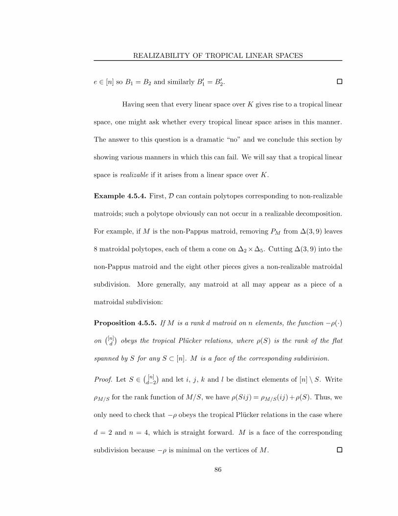
REALIZABILITY OF TROPICAL LINEAR SPACES
e ∈ [n] so B1 = B2 and similarly B′1 = B′
2.
Having seen that every linear space over K gives rise to a tropical linear
space, one might ask whether every tropical linear space arises in this manner.
The answer to this question is a dramatic “no” and we conclude this section by
showing various manners in which this can fail. We will say that a tropical linear
space is realizable if it arises from a linear space over K.
Example 4.5.4. First, D can contain polytopes corresponding to non-realizable
matroids; such a polytope obviously can not occur in a realizable decomposition.
For example, if M is the non-Pappus matroid, removing PM from ∆(3, 9) leaves
8 matroidal polytopes, each of them a cone on ∆2×∆5. Cutting ∆(3, 9) into the
non-Pappus matroid and the eight other pieces gives a non-realizable matroidal
subdivision. More generally, any matroid at all may appear as a piece of a
matroidal subdivision:
Proposition 4.5.5. If M is a rank d matroid on n elements, the function −ρ(·)
on(
[n]d
)
obeys the tropical Plucker relations, where ρ(S) is the rank of the flat
spanned by S for any S ⊂ [n]. M is a face of the corresponding subdivision.
Proof. Let S ∈( [n]d−2
)
and let i, j, k and l be distinct elements of [n] \ S. Write
ρM/S for the rank function of M/S, we have ρ(Sij) = ρM/S(ij)+ρ(S). Thus, we
only need to check that −ρ obeys the tropical Plucker relations in the case where
d = 2 and n = 4, which is straight forward. M is a face of the corresponding
subdivision because −ρ is minimal on the vertices of M .
86
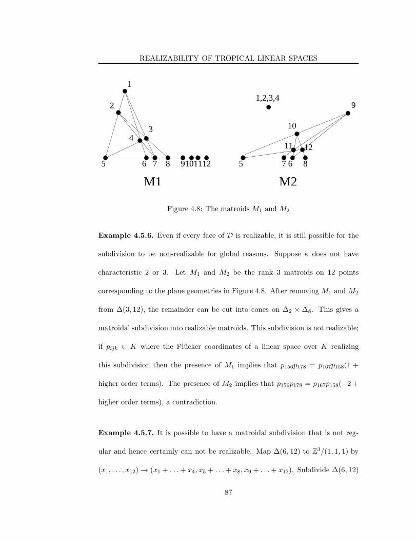
REALIZABILITY OF TROPICAL LINEAR SPACES
M2
1
2
34
5 6 7 8 910 1211
M1
5 87 6
1,2,3,49
10
11 12
Figure 4.8: The matroids M1 and M2
Example 4.5.6. Even if every face of D is realizable, it is still possible for the
subdivision to be non-realizable for global reasons. Suppose κ does not have
characteristic 2 or 3. Let M1 and M2 be the rank 3 matroids on 12 points
corresponding to the plane geometries in Figure 4.8. After removing M1 and M2
from ∆(3, 12), the remainder can be cut into cones on ∆2 × ∆8. This gives a
matroidal subdivision into realizable matroids. This subdivision is not realizable;
if pijk ∈ K where the Plucker coordinates of a linear space over K realizing
this subdivision then the presence of M1 implies that p156p178 = p167p158(1 +
higher order terms). The presence of M2 implies that p156p178 = p167p158(−2 +
higher order terms), a contradiction.
Example 4.5.7. It is possible to have a matroidal subdivision that is not reg-
ular and hence certainly can not be realizable. Map ∆(6, 12) to Z3/(1, 1, 1) by
(x1, . . . , x12) → (x1 + . . .+ x4, x5 + . . .+ x8, x9 + . . .+ x12). Subdivide ∆(6, 12)
87
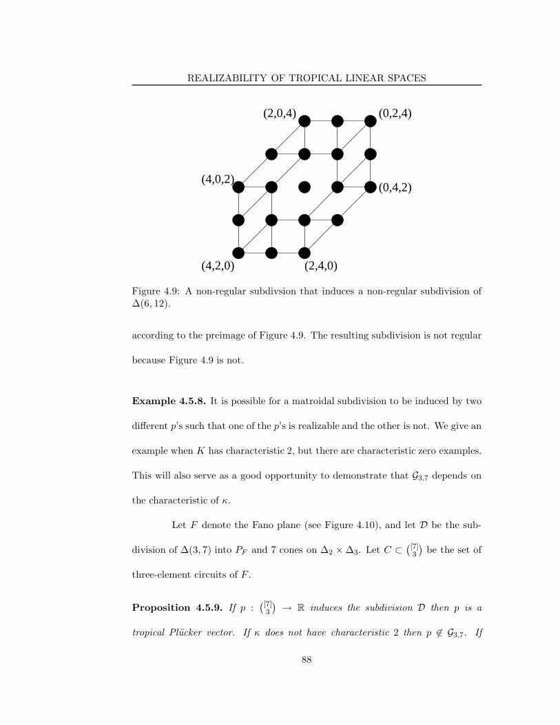
REALIZABILITY OF TROPICAL LINEAR SPACES
(4,2,0) (2,4,0)
(0,4,2)
(0,2,4)(2,0,4)
(4,0,2)
Figure 4.9: A non-regular subdivsion that induces a non-regular subdivision of∆(6, 12).
according to the preimage of Figure 4.9. The resulting subdivision is not regular
because Figure 4.9 is not.
Example 4.5.8. It is possible for a matroidal subdivision to be induced by two
different p’s such that one of the p’s is realizable and the other is not. We give an
example when K has characteristic 2, but there are characteristic zero examples.
This will also serve as a good opportunity to demonstrate that G3,7 depends on
the characteristic of κ.
Let F denote the Fano plane (see Figure 4.10), and let D be the sub-
division of ∆(3, 7) into PF and 7 cones on ∆2 × ∆3. Let C ⊂([7]
3
)
be the set of
three-element circuits of F .
Proposition 4.5.9. If p :([7]
3
)
→ R induces the subdivision D then p is a
tropical Plucker vector. If κ does not have characteristic 2 then p 6∈ G3,7. If
88
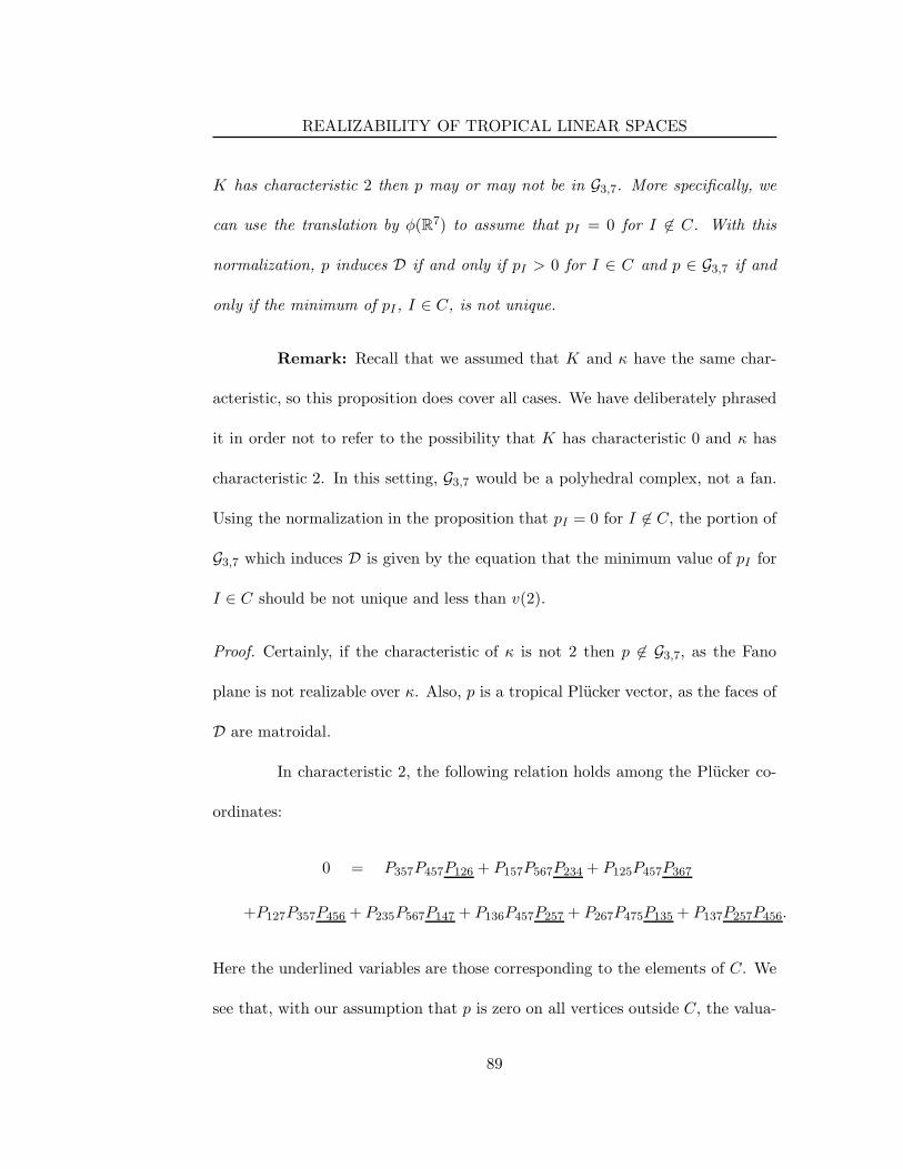
REALIZABILITY OF TROPICAL LINEAR SPACES
K has characteristic 2 then p may or may not be in G3,7. More specifically, we
can use the translation by φ(R7) to assume that pI = 0 for I 6∈ C. With this
normalization, p induces D if and only if pI > 0 for I ∈ C and p ∈ G3,7 if and
only if the minimum of pI , I ∈ C, is not unique.
Remark: Recall that we assumed that K and κ have the same char-
acteristic, so this proposition does cover all cases. We have deliberately phrased
it in order not to refer to the possibility that K has characteristic 0 and κ has
characteristic 2. In this setting, G3,7 would be a polyhedral complex, not a fan.
Using the normalization in the proposition that pI = 0 for I 6∈ C, the portion of
G3,7 which induces D is given by the equation that the minimum value of pI for
I ∈ C should be not unique and less than v(2).
Proof. Certainly, if the characteristic of κ is not 2 then p 6∈ G3,7, as the Fano
plane is not realizable over κ. Also, p is a tropical Plucker vector, as the faces of
D are matroidal.
In characteristic 2, the following relation holds among the Plucker co-
ordinates:
0 = P357P457P126 + P157P567P234 + P125P457P367
+P127P357P456 + P235P567P147 + P136P457P257 + P267P475P135 + P137P257P456.
Here the underlined variables are those corresponding to the elements of C. We
see that, with our assumption that p is zero on all vertices outside C, the valua-
89
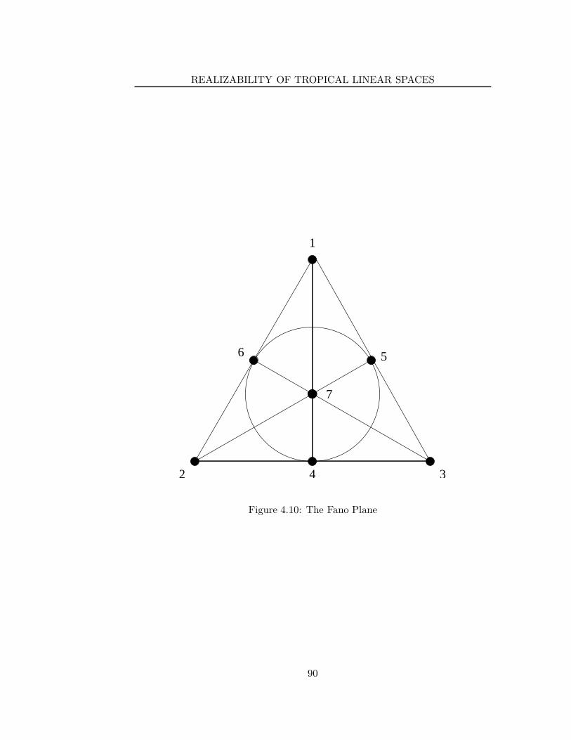
REALIZABILITY OF TROPICAL LINEAR SPACES
1
2 34
56
7
Figure 4.10: The Fano Plane
90
REALIZABILITY OF TROPICAL LINEAR SPACES
tions of the various terms are pI as I runs over C and also p257 + p456. As p257
and p456 > 0, this last term can’t be minimal. We see that the p’s must obey the
relation that the minimum of pI for I ∈ C is not unique in order to be realizable.
Finally, we must show that the condition that minI∈C pI not be unique
is also sufficient. By the symmetry of the problem, we may assume that minI∈C pI
is attained at p456 as well as at PI for some I ∈ C \ 456. Consider
L = RowSpan
1 0 0 atp234 1 1 + ftp367 1
0 1 0 1 + dtp147 btp135 1 1
0 0 1 1 1 + etp257 ctp126 1
.
Here a, b, c, d, e and f are generic members of U = x ∈ K∗ : v(x) = 0.
For I 6∈ C, we have v(PI(L)) = 0. For I ∈ C \ (456), we have
pI(L) = utpI , for some u ∈ U , so v(PI(L)) = pI(L). Finally,
v(P456) = v (atp234 + btp135 + ctp126 + dtp147 + etp257 + ftp367 + · · · )
where the remaining eight terms hidden in the “· · ·” each have valuation at least
as large as 2 minI∈C\(456) pI . If a, b, c, d, e, f are chosen generically, there is
no cancellation, so we have v(P456) = minI∈C\(456) pI = p456 as desired.
We end by discussing two naturally occurring examples of tropical
Plucker coordinates for which I do not know whether or not the corresponding
tropical linear space is realizable.
Problem 4.5.10. Let T be a tree with leaves labeled by [n] and a positive weight
on each edge. For I ⊂ [n], define [I ] to be the minimal subtree of T containing
91
SERIES-PARALLEL MATROIDS AND LINEAR SPACES
I and set pI to be negative the sum of the weights of all edges in [I ]. In [31],
Lior Pachter and I observe that pI are tropical Plucker coordinates; are they
realizable?
Problem 4.5.11. Let R = R((t)). Then R is an ordered field where atα + · · ·
is positive if and only if a is. Thus, it makes sense to define a d × d matrix A
with entries in R to be positive definite if vAvT > 0 for all v ∈ Rd \ 0. Let
X1, . . . , Xn be d× d positive definite symmetric matrices with entries in R. Set
Pi1...id equal to the coefficient of xi1 · · ·xid in det∑
xiXi. The PI do not obey
the Plucker relations. Nonetheless, I show in [37] that v(PI) do obey the tropical
Plucker relations! Are the v(Pi) realizable? If so, give a natural linear space over
R, constructed from the Xi, that realizes them.
4.6 Series-Parallel Matroids and Linear Spaces
Recall that if G is a connected graph (finite, possibly with multiple edges or
loops) then the associated graphical matroid is a matroid whose elements are
the edges of G, whose bases are the spanning trees and whose circuits are the
circuits. See [49], section 6.1 for an overview of graphical matroids. The rank
of this matroid is the number of vertices of G minus one. A matroid is called
series-parallel if it corresponds to a series-parallel graph, i.e. a graph which can
made by starting from a single edge connecting two distinct vertices by repeatedly
applying the series and parallel extension operators. (See Figure 4.11.) For a
92
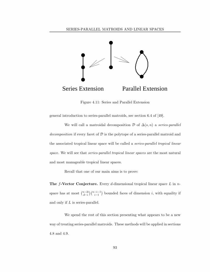
SERIES-PARALLEL MATROIDS AND LINEAR SPACES
Parallel ExtensionSeries Extension
Figure 4.11: Series and Parallel Extension
general introduction to series-parallel matroids, see section 6.4 of [49].
We will call a matroidal decomposition D of ∆(s, n) a series-parallel
decomposition if every facet of D is the polytope of a series-parallel matroid and
the associated tropical linear space will be called a series-parallel tropical linear
space. We will see that series-parallel tropical linear spaces are the most natural
and most manageable tropical linear spaces.
Recall that one of our main aims is to prove:
The f-Vector Conjecture. Every d-dimensional tropical linear space L in n-
space has at most(
n−2id−i
)(
n−i−1i−1
)
bounded faces of dimension i, with equality if
and only if L is series-parallel.
We spend the rest of this section presenting what appears to be a new
way of treating series-parallel matroids. These methods will be applied in sections
4.8 and 4.9.
93
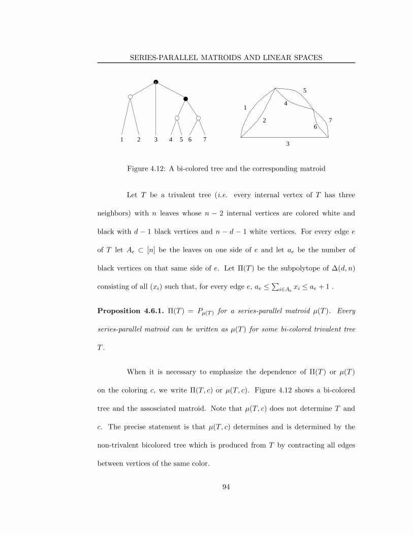
SERIES-PARALLEL MATROIDS AND LINEAR SPACES
4
5
67
1 2 3 4 5 6 7
1
2
3
Figure 4.12: A bi-colored tree and the corresponding matroid
Let T be a trivalent tree (i.e. every internal vertex of T has three
neighbors) with n leaves whose n − 2 internal vertices are colored white and
black with d − 1 black vertices and n − d − 1 white vertices. For every edge e
of T let Ae ⊂ [n] be the leaves on one side of e and let ae be the number of
black vertices on that same side of e. Let Π(T ) be the subpolytope of ∆(d, n)
consisting of all (xi) such that, for every edge e, ae ≤∑
i∈Aexi ≤ ae + 1 .
Proposition 4.6.1. Π(T ) = Pµ(T ) for a series-parallel matroid µ(T ). Every
series-parallel matroid can be written as µ(T ) for some bi-colored trivalent tree
T .
When it is necessary to emphasize the dependence of Π(T ) or µ(T )
on the coloring c, we write Π(T, c) or µ(T, c). Figure 4.12 shows a bi-colored
tree and the assosciated matroid. Note that µ(T, c) does not determine T and
c. The precise statement is that µ(T, c) determines and is determined by the
non-trivalent bicolored tree which is produced from T by contracting all edges
between vertices of the same color.
94
SERIES-PARALLEL MATROIDS AND LINEAR SPACES
Proof. Our proof is by induction on n; when n = 2 the result is clear. Let i
and j ∈ [n] be two leaves of T that border a common vertex v. Define a new
colored trivalent tree T ′ by deleting i and j from T and forgetting the coloring of
v, which is now a leaf. By induction, Π(T ′) = Pµ(T ′) for a series-parallel matroid
µ(T ′).
Case I: v is colored white in T . Then, cutting T at the edge separating i
and j from the rest of T , we see that xi+xj ≤ 1. We define a map φ : Rn → Rn−1
by φ(x)v = xi + xj and φ(x)k = xk otherwise. An easy inspection of the defining
inequalities shows that Π(T ) = ∆(d, n) ∩ φ−1(Π(T ′)). This precisely says that
Π(T ) is the polytope associated to a series extension of µ(T ′) by v.
Case II: v is colored black in T . This is just like the other case except
that xi + xj ≥ 1, we define φ(x)v = xi + xj − 1 and we get a parallel extension.
To show that every series-parallel matroid occurs in this way, reverse
the argument.
Not all of the inequalities above are necessary to define Π(T ). The next
proposition identifies the facets of Π(T ).
Proposition 4.6.2. The facets of Π(T ) are given by (1) the equations∑
i∈Aexe ≥
ae when e is an edge connecting two vertices of the opposite color and Ae is the
set of leaves on the same side of e as the black endpoint, (2) the equations xi ≥ 0
when i is joined to a white vertex and (3) the equations xi ≤ 1 when i is joined to
a black vertex. (All of these are subject to already having the equality∑
xi = d.)
95

SERIES-PARALLEL MATROIDS AND LINEAR SPACES
Proof. We first show that all other equations are redundant. Let e be an internal
edge with Ae and Be the leaves on each side of e and ae and be the number of
black vertices on each side. Then∑
i∈Aexi = d−
∑
i∈Bexi so
∑
i∈Aexi ≤ ae + 1
is equivalent to∑
i∈Bexi ≥ d−(ae +1) = be. If i is a leaf joined to a white vertex
v, let e and e′ be the other two edges issuing from v and let Ae and Ae′ be the
sides of e and e′ not containing v. Then
d = xi +∑
j∈Ae
xj +∑
j∈Ae′
xj ≥ xi + ae + ae′ = xi + d− 1
implying that xi ≤ 1. Similarly, if i is a leaf connected to a black vertex, then
the other inequalities imply xi ≥ 0.
Suppose that e is an internal edge with endpoints u and v, where u is
white. Let e′ and e′′ be the other edges containing u and let Ae, Ae′ and Ae′′
each be as above with Ae on the u side of e and Ae′ , Ae′′ on the non-u side of e′
and e′′. Then
∑
i∈Ae
xe =∑
i∈Ae′
xi +∑
Ae′′
xi ≥ ae′ + ae′′ = ae.
A similar argument show that∑
i∈Aexi ≥ ae is redundant if v is black.
We now must show that each of these inequalities does define a facet.
Our proof is by induction on n. First, consider the inequality∑
i∈Aexe ≥ ae
where e connects a black vertex x to a white vertex y and Ae is on the x side of
e. Let i and j be two leaves of T that border a common vertex v of T . Define T ′
and φ as in the proof of the previous proposition and let x′ be a point of T ′ where
all inequalities except for the one arising from the edge e in T are strict. Then
96
SERIES-PARALLEL MATROIDS AND LINEAR SPACES
any point x obeying φ(x) = x′ and xi, xj ∈ (0, 1) will have all inequalities but
the required one strict. Similar arguments apply to the other inequalities.
We thus see that the facets of Π(T ) which correspond to loop and co-
loop free matroids are in bijection with the edges joining vertices of different
colors, the facets corresponding to matroids with a loop correspond to edges
joining leaves to black vertices and the facets corresponding to matroids with a
co-loop correspond to edges from leaves to white vertices.
Let T be a trivalent tree. Suppose that e is an internal edge. Define T\\e
to be the pair of trivalent trees formed as follows: Let u and v be the endpoints
of e and let a, b, v and c, d, u be the neighbors of u and v respectively. Delete
the vertices u and v and all edges ending at them. Then draw new edges joining
a to b and c to d. If e is an edge joining a leaf i to a vertex v, we define T\\e
similarly except that we simply delete the vertex i. We will use the same notation
F\\e for the analogous construction when F is a forest of trivalent trees and e
an internal edge of a tree of F . If T is colored, we let T\\e inherit the coloring
of T in the obvious way.
Proposition 4.6.3. Let e be an internal edge of T joining two vertices of opposite
colors. Then the corresponding facet of Π(T ) is Π(T1) × Π(T2) where T\\e =
T1 t T2. If e joins a leaf i to a vertex v then the corresponding facet of Π(T ) is
Π(T\\e)× Pi where i is given the structure of a rank 1 matroid if v is black
and a rank 0 matroid if v is white.
97
SPECIAL CASES OF THE F -VECTOR CONJECTURE
The faces of Π(T ) are in bijection with the possible colored forests that
can result from repeated splittings of T along edges connecting vertices of opposite
color or connecting leaves to the rest of T . The faces of Π(T ) that correspond to
loop and co-loop-free matroids are in bijection with the possible colored forests that
can arise by repeated splittings along internal edges between vertices of opposite
color.
Proof. The first paragraph follows because it is easy to check that both polytopes
are defined by the same inequalities. The second paragraph follows by repeatedly
using the first.
4.7 Special Cases of the f-Vector Conjecture
In this section we will prove the following results:
Theorem 4.7.1. Let L be a d-dimensional tropical linear space in n space. Then
L has at most(
n−2d−1
)
vertices, with equality if and only if L is series-parallel.
Theorem 4.7.2. Let L be a d-dimensional tropical linear space in n space with
n = 2d or n = 2d+1. Then L has at most 1 bounded facet if n = 2d and at most
d if n = 2d+ 1.
We first recall the definition of the Tutte polynomial of a matroid. If
M is a rank d matroid on the ground set [n] and Y ⊆ [n], let ρM(Y ) denote the
98
SPECIAL CASES OF THE F -VECTOR CONJECTURE
rank of Y . The polynomial
rM(x, y) =∑
Y ⊆[n]
x|Y |−ρM (Y )yd−ρM (Y )
is known as the rank generating function of M . The polynomial
tM (z, w) = rM(z − 1, w− 1)
is known as the Tutte polynomial of M . Almost all matroid invariants can be
computed in terms of the Tutte polynomial; see Chapter 6 of [50] for a survey
of its importance. Write tM (z, w) =∑
tijziwj . Although not obvious from this
definition, all of the tij are nonnegative. For n ≥ 2 we have t10 = t01, this number
is known as the beta invariant of M and denoted β(M).
We will need the following result:
Proposition 4.7.3. Let M be a matroid on at least 2 elements. Then β(M) = 0
if and only if M is disconnected and β(M) = 1 if and only if M is series-parallel.
Proof. See [10], theorem II, for the first statement and [8], theorem 7.6, for the
second.
The key to proving Theorem 4.7.1 will be proving the following formula:
Lemma 4.7.4. Let M be a matroid and let D be a matroidal subdivision of PM .
Let D denote the set of internal faces of D. Then
tM (z, w) =∑
Pγ∈D
(−1)dim(PM )−dim(Pγ)tγ(z, w).
99
SPECIAL CASES OF THE F -VECTOR CONJECTURE
Before proving Lemma 4.7.4, let us see why it implies Theorem 4.7.1.
Considering the case where M = ∆(d, n) and comparing the coefficients of z on
each side, we see that
β(∆(d, n)) =
(
n− 2
d− 1
)
=∑
γ∈Dγ a facet
β(γ).
(Note that all nonfacets of D correspond to disconnected matroids and hence
have beta invariant 0. and that every facet of D is in D.)
Every term in the right hand sum is a positive integer. Thus, D has at
most(n−2d−1
)
facets, with equality if and only if all of the facets have beta invariant
1, i.e., if and only if D is a decomposition into series-parallel matroids.
We now prove Lemma 4.7.4.
Proof. Since tM (z, w) = rM(z − 1, w− 1), it is enough to prove
rM(x, y) =∑
Pγ∈D
(−1)dim(PM )−dim(Pγ)rγ(x, y).
Plugging in the definition of rM and interchanging summation, it is enough to
show that for every Y ⊆ [n],
x|Y |−ρM (Y )yd−ρM (Y ) =∑
γ∈D
(−1)dim(PM )−dim(Pγ)x|Y |−ργ(Y )yd−ργ(Y ).
Comparing coefficients of x|Y |−ryd−r, we are thus being asked to show
that
∑
Pγ∈Dργ(Y )=r
(−1)dim(PM )−dim(Pγ) =
1 if r = ρM(Y )
0 if r < ρM(Y )
.
100
SPECIAL CASES OF THE F -VECTOR CONJECTURE
The sum is empty if r > ρM(Y ). Equivalently, we will show
∑
Pγ∈Dργ(Y )≥r
(−1)dim(PM)−dim(Pγ) = 1
for all r ≤ ρM(Y ).
Let `Y be the linear function ∆(d, n) → R mapping (xi) 7→∑
i∈Y xi.
Then ργ(Y ) = maxx∈Pγ `Y (x). Thus, we see that ργ(Y ) ≥ r if and only if γ has a
nonempty intersection with the half space `Y > r − 1/2. The promised equality
now follows by the following lemma applied to the polytope PM ∩ x : `Y (x) >
r − 1/2.
Lemma 4.7.5. Let P be any bounded polytope and Γ the internal faces of a
decomposition of P . Then∑
γ∈Γ(−1)dim(P )−dim(γ) = 1.
Proof. This sum is (−1)dimP (χ(P )−χ(∂P )) where χ is the Euler characteristic.
As P is contractible and ∂P is a sphere of dimension dim(P ) − 1, the result
follows.
One might hope to use the higher degree terms of Lemma 4.7.4 to
produce additional bounds on the f -vector of D. Unfortunately, Lemma 4.7.4 is
incapable of producing a complete set of restrictions. For example, consider the
matroids M1, M2 and M3 corresponding to the graphs in Figure 4.13.
The Tutte polynomials of these matroids are
101
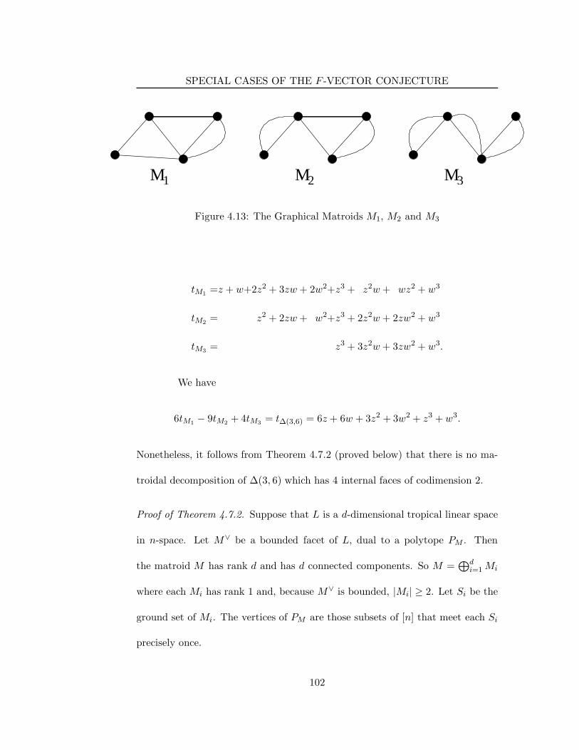
SPECIAL CASES OF THE F -VECTOR CONJECTURE
M M M1 2 3
Figure 4.13: The Graphical Matroids M1, M2 and M3
tM1 =z + w+2z2 + 3zw+ 2w2+z3 + z2w+ wz2 + w3
tM2 = z2 + 2zw+ w2+z3 + 2z2w+ 2zw2 + w3
tM3 = z3 + 3z2w+ 3zw2 + w3.
We have
6tM1 − 9tM2 + 4tM3 = t∆(3,6) = 6z + 6w + 3z2 + 3w2 + z3 + w3.
Nonetheless, it follows from Theorem 4.7.2 (proved below) that there is no ma-
troidal decomposition of ∆(3, 6) which has 4 internal faces of codimension 2.
Proof of Theorem 4.7.2. Suppose that L is a d-dimensional tropical linear space
in n-space. Let M∨ be a bounded facet of L, dual to a polytope PM . Then
the matroid M has rank d and has d connected components. So M =⊕d
i=1Mi
where each Mi has rank 1 and, because M∨ is bounded, |Mi| ≥ 2. Let Si be the
ground set of Mi. The vertices of PM are those subsets of [n] that meet each Si
precisely once.
102
SPECIAL CASES OF THE F -VECTOR CONJECTURE
Now, consider two such facets M∨ and (M ′)∨ occurring in the same
linear space and define Si and S ′i as above. The polytope PM ∩ PM ′ must be
either matroidal or empty.
Lemma 4.7.6. Let Γ = Γ(M,M ′). Γ may have multiple edges, let Γ be the
simple graph obtained by replacing each multiple edge of Γ by a single edge. Then
PM ∩ PM ′ is empty if and only if Γ has no perfect matchings. PM ∩ PM ′ is
matroidal if and only if Γ has precisely one perfect matching.
A perfect matching of a graph Γ is a collection of edges such that, for
every vertex v of Γ, exactly one edge in the collection contains v.
Proof. The vertices of PM ∩ PM ′ are in bijection with the perfect matchings of
Γ. There is an obvious surjection from perfect matchings of Γ to matchings of Γ.
This proves the first claim.
Suppose that PM ∩ PM ′ is nonempty and matroidal. Let (B1, B2) be
an edge of PM ∩ PM ′ , so B1 and B2 correspond to perfect matchings of Γ that
differ only by a single edge say B1 \ e1 = B2 \ e2. Then e1 and e2 have the
same image in Γ in order for both B1 and B2 to be perfect matchings. Since
every pair of vertices of PM ∩ PM ′ is connected by a chain of edges, we see that
every perfect matching of Γ gives rise to the same perfect matching of Γ or, in
other words, Γ has exactly one perfect matching. Conversely, if Γ has exactly one
perfect matching, it is clear that PM ∩ PM ′ is a product of simplices and hence
matroidal.
103
SPECIAL CASES OF THE F -VECTOR CONJECTURE
We now turn to the cases we are interested in, when n = 2d or 2d+ 1.
We maintain the notation of the lemma. First, suppose that n = 2d. Then every
Si must have order 2 so, for any Si and S ′i, the graph Γ must consist of disjoint
cycles. The only way that Γ can be a forest is if all of those cycles have length 2.
But then Si = Ti. So we see that a linear space of dimension d in 2n space
can have at most one bounded facet.
Now suppose that n = 2d + 1. Then all of the Si have order 2 except
for one which has order 3. We order the Si so that |S1| = 3. Γ consists of several
disjoint cycles and one component C. C consists of a pair of vertices v and w
of degree 3 with opposite colors and three disjoint paths γ1, γ2, γ3. Either these
paths all run from v to w or there is one path each running from v to v, from v
to w and from w to w.
In any of these cases, Γ has at least one perfect matching. One can
check that the only case where Γ has only one perfect matching is when all of the
cycles of Γ \C have length 2 and C consists of a path from v to w and two cycles
of length 2, one containing v and the other containing w. The second condition
is equivalent to requiring that S ′i′ ⊂ S1 and Si ⊂ S ′
1 for some i and i′.
Consider all of the three element subsets of [n] that occur as an S1 for
some bounded facet of L. We first note that, if S1 = S ′1 then Si = S ′
i for every i
(after reordering) as otherwise Γ would have a cycle of length more than 2. So
all of the Sr1 subsets are different.
104
SPECIAL CASES OF THE F -VECTOR CONJECTURE
Let f be the number of bounded facets of L with (Sr1, S
r2, . . . , S
rd) the
partition of [n] corresponding to the rth facet of L for 1 ≤ r ≤ f . We now build a
graph whose vertices are the various Sr1 and the labels 1, . . . , n. Let there be an
edge between Sr1 and k if k ∈ Sr
1. This graph has f+n = f+2d+1 vertices and 3f
edges. Thus, if f > d, this graph has as many edges as vertices and must contain
a cycle, we will use this cycle to obtain a contradiction. Saying this graph has a
cycle means that there exist i1, . . . , ig, j1, . . . , jg ∈ [n] and facets corresponding
to collections (Srs), 1 ≤ s ≤ d, 1 ≤ r ≤ g such that Sr
1 = ir, ir+1, jr, where the
index r is cyclic modulo g.
Now, for any r and r′, there must be some Srs ⊂ Sr′
1 . Consider first
the case where r′ = r + 1. Then jr+1, ir+2 must be one of the Srs , as we
already know ir+1 ∈ Sr1 . Now consider when r′ = r+ 2. We get that jr+2, ir+3
must be one of the Srs , as ir+2, the other member of Sr′
1 , is already contained in
jr+1, ir+2. Continuing in this manner, we get that jr+k, ir+k+1 is an Srs for
every k. But, when k = g − 1, this intersects Sr1 , contradicting that the Sr
i are
distinct.
The f -vector conjecture predicts that, if n = 2d+ e, L should have at
most(
d+e−1e
)
bounded facets. In the cases e = 0 and e = 1, the graph Γ always
has at least one matching and the requirement that Γ have exactly one is very
restrictive. Once e = 2, it is possible for Γ to have no perfect matchings and the
105
RESULTS ON CONSTRUCTIBLE SPACES
problem grows much harder.
Nonetheless, I suspect that this kind of reasoning, looking only at the
facets of L and not at the smaller spaces that contain them, is adequate to resolve
the f -vector conjecture for facets once e ≥ 2. More specifically, I conjecture:
Conjecture 4.7.7. Let n = 2d+ e. It is not possible to find more than(
d+e−1e
)
distinct partitions of [n] into d disjoint subsets, [n] = Sr1 t · · ·tSr
d where each Srs
has order at least 2 and, for every r and r′, the graph Γ formed from Sr1, . . . , S
rd
and Sr′1 , · · · , S
r′
d has at most one perfect matching.
Remark: Consider the case where d = 3. In this case, there is an
elegant way to describe the compatability condition between (S1, S2, S3) and
(S ′1, S
′2, S
′3). Two partitions of [n] into triples (S1, S2, S3) and (S ′
1, S′2, S
′3) are
compatible if and only if, after reordering the Si and S ′i, we have S1 ⊆ S ′
1 and
S3 ⊇ S ′3.
4.8 Results on Constructible Spaces
In this section, we will prove several of the previously stated results on con-
structible spaces. Our first aim is to prove Theorem 4.1.3: that every con-
structible space is series-parallel. Clearly, L⊥ is series-parallel if L is, since the
dual of a series-parallel matroid is series-parallel. So it is enough to show that,
if L and L′ are two series-parallel tropical linear spaces that meet transversely
then L ∩ L′ is series-parallel as well.
106
RESULTS ON CONSTRUCTIBLE SPACES
Let L and L′ be two tropical linear spaces of dimensions d and d′ in n
space which meet transversely at a point w. Let D and D′ be the appropriate
subdivisions of ∆(d, n) and ∆(d′, n). Let M∨ and (M ′)∨ be the faces of D∨ and
(D′)∨ containing w. Let M =⊕
i∈I Mi and M ′ =⊕
i∈I ′ M′i be the connected
components of M and M ′. We claim that all of the Mi and M ′i are series-parallel.
PM will be a face of some facet PM of D, so this follows from
Lemma 4.8.1. Let M be a series-parallel matroid and let PM be a face of PM ,
assume that M is loop-free. Let M =⊕
Mi be the decomposition of M into
connected components. Then each of the Mi are series-parallel.
Proof. This follows from the description of the faces of M in Lemma 4.6.3. (Note
that a rank one matroid on a single element is series-parallel.)
The result now follows from
Proposition 4.8.2. Let M =⊕
Mi and M ′ =⊕
M ′i be transverse matroids on
[n] with all of the Mi and M ′i series-parallel. Then M ∧M ′ is a direct sum of
series-parallel matroids, and is series-parallel if it is connected.
Proof. M ∧ M ′ is formed by a sequence of parallel connections. The parallel
connection of two series-parallel matroids is series-parallel.
Our next goal is to prove Theorem 4.1.2 – every constructible space
achieves the f -vector of the f -vector conjecture. Our strategy is as follows: A
constructible space is made by succesive dualization and transverse intersection.
107
RESULTS ON CONSTRUCTIBLE SPACES
It is easy to show that dualization preserves the f -vector, so our main goal is to
understand the effect of transverse intersection.
We will first prove (Theorem 4.8.4) that, if L and L′ are series-parallel
tropical linear spaces and v ∈ Rn, then the f -vector of L∩(L′+v) is independent
of v as long as we impose that L and L′+v meet transversely. The most technical
part of this proof is the analysis of perturbing L′ slightly when L and L′ are almost
transverse, this is carried out in Lemma 4.8.5. Our result ultimately relies on a
lemma (Lemma 4.8.3) about chains of flats in series-parallel matroids.
Once we have proven that the f -vector of L ∩ (L′ + v) is independent
of v, we find a particular value of v for which this f vector is particularly easy
to compute. The computation involves several binomial coefficient identities.
Lemma 4.8.3. Let M be a series-parallel matroid. Call a flat Q of M a flacet
if M |Q and M/Q are connected. Let f and g ∈ M . Then the collection of all
flacets Q such that f ∈ Q and g 6∈ Q forms a chain Q1 ⊂ · · · ⊂ Qd. Moreover,
the length d of this chain is preserved when the roles of f and g are switched.
We define d(f, g) to be d.
Remark: The terminology “flacet” was suggested by Bernd Sturmfels.
The motivation for this terminology is that, for M any connected matroid, the
flacets of M are in bijection with the facets of PM .
Proof. As remarked above, if Q is a flacet then M |Q ⊕M/Q corresponds to a
facet of M . Let M = µ(T ). By Lemma 4.6.3, all of the facets of PM correspond
108
RESULTS ON CONSTRUCTIBLE SPACES
to either edges of T which contain a leaf or edges of T that connect to vertices
of opposite colors. Under that correspondence, an edge e corresponds to a flacet
that contains f and not g if and only if e separates f and g with the end closer to g
colored black and the end closer to f either colored white or equal to e. Consider
the path γ through T connecting f and g, divide γ into alternating blocks of
white and black vertices. Then we see that the number of flacets containing f
and not g is equal to the number of black blocks. This number is the same when
f and g are switched. The flat corresponding to e consists of the leaves of T that
are on the non-black end of e. Thus, all of the flats in question are nested.
Our first major goal on the way to proving Theorem 4.1.2, nontrivial in
its own right, is to prove:
Theorem 4.8.4. Let L and L′ be two series-parallel tropical linear spaces in
n-space, of dimensions d and d′. Let a and b ∈ Rn be such that L meets L′ + a
and L′+b transversely. Then L∩(L′ +a) and L∩(L′ +b) have the same bounded
f -vector.
We first prove a lemma describing what happens when we perturb a
non-transverse intersection of two tropical linear spaces.
Let L and L′ be tropical linear spaces of dimensions d and d′. Let 0
be a vertex of L ∩stable
L′ and let M =⊕
i∈I Mi and M ′ =⊕
i′∈I ′ M′i′ be the
matroids such that 0 lies in the relative interiors of M∨. Let E be the subdivision
of ∆(d+ d′, n) corresponding to L ∩stable
L′, so PM∧M ′ is a face of E with 0 in the
109
RESULTS ON CONSTRUCTIBLE SPACES
relative interior of (M ∧M ′)∨.
Let v be a generic vector of Rn and consider the tropical linear space
L ∩stable
(L′+v) = L∩(L′+v). The tropical linear space L ∩stable
(L′+v) corresponds
to a matroidal subdivision Ev of ∆(d + d′, n). We will describe the facets into
which the relative interior of PM∧M ′ is divided in Ev.
Let T be a tree and π : T → Γ(M,M ′) a map of graphs which is bijective
on edges. (Note: since we assumed that (M ∧M ′)∨ was a vertex of L ∩stable
L′,
we know that Γ(M,M ′) is connected.) Let u be a real valued function on the
vertices of T all of whose values are distinct. Let i be a vertex of Γ(M,M ′). Let
j1, l . . . , jr = π−1(i) ordered so that u(j1) < u(j2) < · · ·< u(jr).
Recall that S(′)i is the set of edges ending at vertex i and has the matroid
structure M(′)i placed on it. Let Qk be the subset of S
(′)i consisting of those edges
whose preimage in F has endpoint jk′ for some k′ ≤ k. ThusQ1 ⊂ Q2 ⊂ · · · ⊂ Qk.
Place the matroid structure M(′)i |Qk
/Qk−1 on the edges of T coming into vertex
jk . (We adopt the convention that Q0 is the empty set.)
Now T is a tree where, at every vertex, the structure of a matroid has
been assigned to the edges ending at that vertex. We denote by µ(M,M ′, T, π, u)
the matroid formed by taking parallel connections along the edges of T as in
Section 4.4.
Lemma 4.8.5. With the above notation, and for v sufficiently small, every facet
of Ev contained in the relative interior of PM∧M ′ is of the form µ(M,M ′, T, π, u)
110
RESULTS ON CONSTRUCTIBLE SPACES
for some T , π and u. More specifically, µ(M,M ′, T, π, u) occurs in E if and only
if
1. For every vertex i of Γ(M,M ′) and for every jk ∈ π−1(i), the matroid
M(′)i |Qk
/Qk−1 is connected.
2. For every edge e = (i, i′) of T with π(i) ∈ I and π(i′) ∈ I ′, we have
v(π(e)) = u(i)−u(i′). Here v ∈ Rn is thought of as a function on the edges
of Γ(M,M ′).
More generally, suppose that (M ∧ M ′)∨ is an i-dimensional face of
L ∩stable
L′ (equivalently, if Γ(M,M ′) has i connected components). Then PM∧M ′
is subdivided in Ev into facets. These facets are described by giving a forest F , a
map π : F → Γ(M,M ′) in which the preimage of each component of Γ(M,M ′)
is a tree and a function u on the vertices of F which obeys the hypotheses above.
We use the notation µ(M,M ′, F, π, u) in this situation.
Remark: The assumption that M(′)i |Qk
/Qk−1 is loop-free is equivalent
to assuming that Qk−1 is a flat of M(′)i |Qk
. Assuming that M(′)i |Qk
/Qk−1 is loop-
free for all k is thus equivalent to assuming that Q1 ⊂ Q2 ⊂ · · · ⊂ Qk is a chain
of flats of M(′)i .
Proof. Every face of L ∩ (L′ + v) is the intersection of a face R∨ of L and a face
(R′)∨ + v of L′ + v. This matroid corresponding to said face of L ∩ (L′ + v) is
R ∧R′. If this face is dual to one of the face appearing in the subdivision of the
111

RESULTS ON CONSTRUCTIBLE SPACES
relative interior of PM∧M ′ then M∨ ⊂ R∨ and (M ′)∨ ⊂ (R′)∨. That M∨ ⊆ R∨
means that R is of the form⊕
Qk/Qk−1 for Q· a chain of flats in M . Similarly,
R′ =⊕
Q′k/Q
′k−1 for Q′
· a chain of flats in M ′. By refining the chains Q(′)· , we
may assume that each succesive quotient Q(′)k /Q
(′)k−1 is connected.
Let T be the graph Γ(R,R′). Since we are looking for facets of Ev, we
have that R∧R′ is connected so T is connected. The fact that the faces R∨ and
(R′)∨ + v meet for generic v means that T is acyclic. Thus, T is a tree. We have
a map π : Γ(R,R′) → Γ(M,M ′) which sends Q(′)k /Q
(′)k−1 to the unique connected
component of M (′) which contains all the members of the set Q(′)k \Q
(′)k−1. This
map is bijective on edges. (Both edge sets are naturally labelled with [n] and
this map preserves the labelling.) Find a real valued function u on the vertices
of T such that u orders the vertices above each i ∈ I ∪ I ′ correctly and we will
have µ(M,M ′, T, π, u) = R ∧R′.
Now, not every µ(M,M ′, T, π, u) occurs because sometimes the relative
interiors of R∨ and (R′)∨ + v are disjoint. We must determine when the relative
interiors of R∨ and (R′)∨ + v meet. For v small enough, this is equivalent to
determining when v is in the relative interior of the sum of the local cones at 0
of R∨ and −(R′)∨. The local cone of R is spanned by all vectors x ∈ Rn with x
constant on the set Qk \Qk−1 and x(Qk \Qk−1) < x(Qk+1\Qk). (See Proposition
4.2.3.) Such a vector x gives rise to a function u on π−1(I), where u(j) = x(e) for
any edge e ending at j. Similarly, we can use a point of the local cone of −(R′)∨
112
RESULTS ON CONSTRUCTIBLE SPACES
to define a function u on π−1(I ′). We thus see that the condition that v lie in
the relative interior of the sum of the local cones of R∨ and −(R′)∨ implies that
the function u obeys condition (2) above. We have thus shown that every facet
into which the relative interior of PM∧M ′ is divided arises in the above manner.
It is easy to reverse this argument and show that if T , π and u meet the
conditions above then the faces R∨ and R∨ + v do meet. The face given by the
intersection is dual to the matroid R ∧R′, which is formed by contracting along
the edges of T (see Lemma 4.4.3). As v approaches 0, the vertex R∨ ∩ (R∨ + v)
approaches (M ∧M∨). This tells us that PR∧R′ appears in the relative interior
of PM∧M ′.
There is no difficulty except for additional bookkeeping in the case where
M ∧M ′ has multiple components.
Remark: I haven’t found a comparably simple dsescription of the lower
dimensional faces into which the relative interior PM∧M ′ is dubdivided. The most
obvious guess is to replace the tree T with a forest. This winds up describing the
faecs of Ev contained in PM∧M ′, but it describes both the faces in the relative
interior of PM∧M ′ ans the boundary. The trouble is that, as v approaches 0,
R∨∩ (R∨ +v) may shrink down to the vertex (M ∧M ′)∨ or it may remain higher
dimensional and approach a face which contains (M ∧M ′)∨ in its boundary. In
the setting of the lemma, R∨ ∩ (R∨ + v) is already a vertex, so this issue doesn’t
arise.
113

RESULTS ON CONSTRUCTIBLE SPACES
We now prove Theorem 4.8.4.
Proof of Theorem 4.8.4. Let Ui ∈ Rn be the set of v such that, for any two faces
F and F ′ of L and L′, either the relative interiors of F and F ′ + v are disjoint
or they span an affine linear space of dimension at least n − i. Thus, L and
L′ + v meet transversely if and only if v ∈ U0. Rn \Ui is a polyhedral complex of
dimension at most n− i− 1. In particular, we see that U1 is path connected. We
may therefore join a and b by a path through U1. It is thus enough to show that,
if v ∈ U1 \ U0 and we perturb v into U0 then the f -vector we get is independent
of the choice of perturbation. Without loss of generality, we may assume that
v = 0.
Let N∨ be a face of L ∩stable
L∨ at which two faces M∨ and (M ′)∨ fail to
meet transversely. Let the connected components of M and M ′ be⊕
i∈I Mi and
⊕
i∈I ′ M′i .
In our setting, sinceM∨ and (M ′)∨ span an affine hyperplane, Γ(M,M ′)
will have first Betti number 1 and will thus contain a unique cycle. Let e1, . . . ,
e2r be the edges of that cycle in cyclic order. Write ij and ij+1 for the ends of ej
with ij ∈ I for j odd and ij ∈ I ′ for j even. Let G be the component of Γ(M,M ′)
containing this cycle.
Now, let v ∈ Rn be generic and sufficiently small and let Ev be the
decomposition of ∆(d+d′−n, n) associated to L ∩stable
(L′+v). Eεv is a subdivision
of E0. We will show that the number of faces of codimension c into which the
114
RESULTS ON CONSTRUCTIBLE SPACES
relative interior of PN is subdivided is independent of v. We will first compute
this number on the assumption that∑2r
s=1(−1)sves > 0. We will then recompute
it on the assumption that∑2r
s=1(−1)sves < 0 and see that we get the same answer.
We first consider the facets into which PN is subdivided. In the notation
of Lemma 4.8.5, every face of Ev is of the form µ(M,M ′, F, π, u). The map
π : F → Γ(M,M ′) must be an isomorphism on every component of Γ(M,M ′)
except G and must be bijective on G except for a single vertex is somewhere in
the loop of G whose preimage is two vertices. Let j1 and j2 be the two preimages
of is, with the preimage of edge es−1 ending at j1 and the preimage of es ending
at j2.
Suppose that s is odd, so is ∈ I . Then condition (2) of Lemma 4.8.5
gives us
u(j1) − u(j2) =(
u(j1)− u(π−1(is−1)))
+(
u(π−1(is−1))− u(π−1(is−2)))
+ · · ·
+(
u(π−1(is+1)) − u(j2))
= v(es−1)− v(es−2) + · · · − v(es)
=
2r∑
s=1
(−1)sves > 0.
115

RESULTS ON CONSTRUCTIBLE SPACES
If s is even, so is ∈ I′, then we have
u(j1) − u(j2) =(
u(j1)− u(π−1(is−1)))
+(
u(π−1(is−1))− u(π−1(is−2)))
+ · · ·
+(
u(π−1(is+1)) − u(j2))
= −v(es−1) + v(es−2) − · · ·+ v(es)
=
2r∑
s=1
(−1)sves > 0.
Either way, u(j1) > u(j2). So, in order to be in accord with condition (1) of
Lemma 4.8.5, we must have that the edges coming into j1 must form a flat Q
of M(′)is
and M(′)is|Q and M
(′)is/Q must both be connected. In other words, Q
must be a flacet of M(′)is/Q. For each flacet of M
(′)is
which contains es−1 and
not es, we get a facet of Ev. Thus, we see that the number of facets of Ev into
which PN is subdivided is D :=∑2r
s=1 d(es−1, es). If we redo this computation
on the assumption that∑2r
s=1(−1)sves < 0, we see that the number of facets into
which PN is subdivided is∑2r
s=1 d(es, es−1) which, by Lemma 4.8.3, is the same
as∑2r
s=1 d(es−1, es).
We now consider instead the problem of determining the number of
codimension c faces into which the relative interior of PN is subdivided in Ev.
Each such face is an intersection of facets of Ev in the relative interior of PN .
Once again, we start our discussion on the assumption that∑2r
s=1(−1)sves > 0.
We claim that every c+ 1 element subset of the D facets of Ev found above has
a distinct, nonempty intersection in the interior of PN . Thus, there are( Dc+1
)
codimension c faces and this number would be the same if∑2r
s=1(−1)sves < 0.
116
RESULTS ON CONSTRUCTIBLE SPACES
To give a facet of Ev is to give a choice of an integer s between 1 and
2r and a flacet Q of M(′)is
which contains es−1 and not es. To give c + 1 such
facets we must give, for each s a collection Q1s , . . . , Qc2r
2r of flacets with each Qts
containing es−1 and not es, where∑
cs = c+ 1. By Lemma 4.8.3, Q1s , . . . , Qc2r
2r
will form a nested chain and we may reorder them such that Q1s ⊂ · · · ⊂ Qc2r
2r .
We can find a c-tree forest F with a surjection π onto Γ(M) where is has cs
preimages and the edges coming into the tth preimage of is are labelled by the
elements of the set Qts \Q
t−1s . Let S be the matroid formed by making parallel
connections along the edges of F . All of the facets meet at PS . One can check
that PS meets the relative interior of PN . The same argument goes through with
es and es−1 reversed when∑2r
s=1(−1)sves < 0.
Remark: As v goes to 0, (L ∩ (L′ + v))/(1, . . . , 1) has a (D − 1)-
dimensional simplex which shrinks down to a point at v = 0. After∑2r
s=1(−1)sves
changes sign, a new (D− 1)-dimensional simplex begins to grow.
We now are ready to begin our final assault on Theorem 4.1.2. We
will first need to study how the various faces of ∆(d, n) are subdivided in a
constructible decomposition. Let S and T be disjoint subsets of [n]. Write
∆(d, n) \ S/T for the face of ∆(d, n) given by the equations xi = 0 for i ∈ S and
xi = 1 for i ∈ T . If p is a tropical Plucker vector then define p \ S/T to be the
function on the vertices of ∆(d−|T |, n−|S|− |T |) given by (p\S/T )I = pI∪T . It
is clear that p \ S/T obeys the tropical Plucker relations, as they are a subset of
117
RESULTS ON CONSTRUCTIBLE SPACES
the tropical Plucker relations for p. So p \ S/T corresponds to a tropical d− |T |
plane in n − |S| − |T | space. If L is the tropical linear space corresponding to p
then we write L \ S/T for the tropical linear space corresponding to p \ S/T .
Lemma 4.8.6. If L is a constructible d-plane in n-space and S and T are disjoint
subsets of [n] then L \ S/T is also constructible.
Proof. If L is a hyperplane then every L\S/T is either a hyperplane or the whole
space in which it sits, and hence is constructible. Now suppose that the lemma
holds for L. Then it holds for L⊥ as L⊥ \ S/T = (L \ T/S)⊥. Suppose that the
lemma holds for L and L′. Then it holds for L ∩stable
L′ as (L ∩stable
L′) \ S/T =
(L \ ∅/(S ∪ T )) ∩stable
(L′ \ S/T ).
Proof of Theorem 4.1.2. Our proof is by induction, first on n and then on the
number of steps used to construct L. We set
fi,d,n =
(
n− 2i
d− i
)(
n− i− 1
i− 1
)
=(n− i− 1)!
(i− 1)!(d− i)!(n− d− i)!.
First, suppose that the theorem is true for L. L⊥ and L have the same
bounded f -vector, so the theorem for L⊥ follows from the symmetry fi,d,n =
fi,n−d,n. For the rest of the proof, suppose that L and L′′ are a constructible
d-plane and d′ plane in n space which meet transversely and for which we know
the theorem to hold. In addition, we know that the theorem holds for every
L \S/T and L′′ \S/T by our inductive hypothesis. Our aim will be to prove the
theorem for L ∩ L′′.
118
RESULTS ON CONSTRUCTIBLE SPACES
By Theorem 4.8.4, it is enough to prove the result for L∩(L′′+w) where
w is chosen generically enough. We will take a w for which w1 w2 · · · wn
and otherwise generic. Set L′ = L′′ + w.
Suppose that M∨ is a face of L dual to PM ⊂ ∆(d, n). Then M is loop-
free, let T be the set of co-loops of M so that M lies in the relative interior of
∆(d, n)\∅/T . Then M∨/(1, . . . , 1) is the product of RT+ and a bounded polytope.
Let (M ′′)∨ be a face of L′′ and define T ′ similarly. We write (M ′)∨ = (M ′′)∨ +w
and M ′ = M ′′.
Define an ordered pair (T, T ′) of subsets of [n] to be nice if, for all
1 ≤ i < j ≤ n, either j ∈ T or i ∈ T ′.
Lemma 4.8.7. For w1 w2 · · · wn, we have M∨ ∩ (M ′)∨ 6= ∅ if and only
if (T, T ′) is nice. If (T, T ′) is nice then M∨ ∩ (M ′)∨ is bounded if and only if
T ∩ T ′ = ∅.
.
Proof. First, suppose that (T, T ′) is not nice, so there exists some i < j with
j 6∈ T and i 6∈ T ′. On M∨, the function xj − xi is bounded above (as j 6∈ T ).
On (M ′′)∨, xj − xi is similarly bounded below. The value of xj − xi on (M ′′)∨
is wj −wi larger than on (M ′′)∨, so if wj −wi is large enough then the values of
this functional on M∨ and (M ′′)∨+w will be distinct. Thus, M∨ and (M ′′)∨+w
will be disjoint.
Now suppose that (T, T ′) is nice. Let (xi) ∈M∨ and (x′′i ) ∈ (M ′′)∨, set
119

RESULTS ON CONSTRUCTIBLE SPACES
x′i = x′′i +wi and set di = x′i−xi. For w large enough, we have d1 < d2 < · · ·< dn.
The hypothesis that (T, T ′) is good implies that there is some b ∈ [n] such that
i ∈ T ′ for every i < b and j ∈ T ′ for every j > b. After translating (xi) by
(1, . . . , 1), which will not change the assumption that (xi) ∈M , we may assume
that xb = x′b. Consider the point
z := (x1, . . . , xb−1, xb, xb+1 + db+1, . . .xn + dn)
(x′1 − d1, . . . , x′b−1 − db−1, x
′b, x
′b+1, . . .x
′n).
Clearly, z ∈ (xi) + RT≥0 and z ∈ (x′i) + RT ′
≥0, so z ∈ M∨ ∩ (M ′)∨. We have now
proved the first claim.
Now assume that (T, T ′) is nice, so there is some point z = (zi) ∈
M∨ ∩ (M ′)∨. Suppose that i ∈ T ∩ T ′. Then z + uei ∈ M∨ ∩ (M ′)∨ for every
u > 0 and M∨ ∩ (M ′)∨ is unbounded.
Suppose, on the other hand, that T ∩ T ′ = ∅. Consider any i < j. If
neither i nor j is in T then xi − xj is bounded on M∨; if neither i nor j is in T ′
then xi − xj is bounded on (M ′)∨; if j ∈ T and i ∈ T ′ then xi − xj is bounded
above on M∨ and below on (M ′)∨. In any of these cases, we see that xi − xj
is bounded on M∨ ∩ (M ′)∨. So all of the xi − xj are bounded on M∨ ∩ (M ′)∨
which implies that (M∨ ∩ (M ′)∨)/(1, . . . , 1) is bounded.
M∨ corresponds to a bounded face of L \ ∅/T . Writing t = |T |, if
this bounded face is j-dimensional then M∨ is (j + t)-dimensional. Similarly
120
RESULTS ON CONSTRUCTIBLE SPACES
writing t′ = |T ′| and j ′ for the dimension of the face of L′ \∅/T ′ corresponding to
(M ′)∨, the dimension of (M ′)∨ is j ′ + t′. The dimension of M∨ ∩ (M ′)∨ is then
j + j ′ + t+ t′ − n. We thus see that the number of i-dimensional bounded faces
of L ∩ L′ is
∑
(T,T ′) niceT∩T ′=∅
∑
j+j′+t+t′−n=i
fj,d−t,n−tfj′ ,d′−t′,n−t′ .
We have used our inductive assumption that all of the tropical linear spaces
L \ ∅/T and L′ \ ∅/T ′ have the correct f -vector.
The only nice pairs (T, T ′) with T ∩ T ′ = ∅ are (1, . . . , b − 1, b +
1, . . . , n) and (1, . . . , b, b+ 1, . . . , n). So we can write this sum as
∑
b
∑
j+j′=i+1
fj,d−b+1,n−b+1fj′ ,d′−n+b,b +∑
j+j′=i
fj,d−b,n−bfj′,d′−n+b,b
.
We will now show that this sum is fi,D,n, where D is d+ d′ − n.
We work with the first sum first. Plugging in the definition fi,d,n =
(
n−d−1i−1
)(
n−i−1n−d−1
)
and exchanging order of summation, we have
∑
j+j′=i+1
(
n − d− 1
j − 1
)(
n− d′ − 1
j ′ − 1
)
∑
b
(
n− b− j
n− d− 1
)(
b− j ′ − 1
n− d′ − 1
)
.
Using the identity∑
k+k′=p
(
kq
)(
k′
r
)
=(
p+1q+r+1
)
, the inner sum evaluates
to(
n−i−12n−d−d′−1
)
=(
n−i−1n−D−1
)
. We are reduced to
(
n − i− 1
n−D − 1
)
∑
j+j′=i+1
(
n − d− 1
j − 1
)(
n − d′ − 1
j ′ − 1
)
.
The remaining sum can be evaluated by the identity∑
j+j′=r
(
pj
)(
qj′
)
=(
p+qr
)
.
We get(
n−i−1D−i
)(
n−D−2i−1
)
.
121
TREE TROPICAL LINEAR SPACES
A similar argument shows that the second sum is(n−i−1
D−i
)(n−D−2i−2
)
.
Adding these together, we get
(
n− i− 1
D − i
)[(
n −D − 2
i− 1
)
+
(
n−D − 2
i− 2
)]
=
(
n− i− 1
D − i
)(
n −D − 1
i− 1
)
= fi,D,n.
4.9 Tree Tropical Linear Spaces
In this section, we will describe some tropical linear spaces which achieve the
bounds of the f -vector conjecture and have very elegant combinatorics. Suppose
that pij obeys the tropical Plucker relations so by the results in the preceding
chapter pij corresponds to a tropical 2-plane L and to a tree T . We define a real
valued function τd(p) on([n]
d
)
by τd(p)I =∑
i,j∈Ii<j
pij .
Proposition 4.9.1. τd(p) obeys the tropical Plucker relations.
This can be checked in a routine manner, but we give a different proof
that explains the motivation behind the formula. We will call the tropical linear
space associated to τd(p) the dth tree space of L and denote it τd(L).
Proof. We know that pij is realizable, meaning that we can find x1, . . .xn, y1,
122
TREE TROPICAL LINEAR SPACES
. . . , yn ∈ K such that pij = v(xiyj − xjyi). Consider the linear space
RowSpan
xd−11 xd−1
2 xd−13 · · · xd−1
n
xd−21 y1 xd−2
2 y2 xd−23 y3 · · · xd−2
n yn
......
... · · ·...
yd−11 yd−1
2 yd−13 · · · yd−1
n
The maximal minor Pi1 ,...,id of this matrix is the Vandermonde deter-
minant det(xd−sir
ys−1ir
) =∏
ir<is(xiryis − xisyir). So
v(PI) =∑
i,j∈Ii<j
v(xiryis − xisyir ) =∑
i,j∈Ii<j
pij = τd(p)I .
So the τd(p)I come from an actual linear space and hence obey the tropical
Plucker relations.
Remark: This construction is reminiscent of the construction of cyclic
polytopes (see, for example, [51] example 0.6) and osculating flags (see [36],
section 5), two other objects which realize maximal combinatorics.
In this section, we will give a complete description of the bounded part
of τd(L) in terms of the combinatorics of T . We will make heavy use of the
results of Section 4.6. From now on, we assume that T is trivalent.
Theorem 4.9.2. The vertices of τd(L) are of the form µ(T, c)∨ where c ranges
over the(
n−2d−1
)
ways to color the internal vertices of T black and white with d− 1
colored black and n − d − 1 colored white. The bounded i-dimensional faces of
τd(T ) are in bijection with the ordered pairs (F, c), where F is a forest with i
123
TREE TROPICAL LINEAR SPACES
trees that can be obtained by splitting T along internal edges and c is a black and
white coloring of the internal vertices of F using d− i black vertices and n−d− i
white vertices. (F, c) is contained in (F ′, c′) if and only if (F ′, c′) can be obtained
from (F, c) by repeated splitting along edges connecting vertices of opposite colors.
Proof. It is enough to prove the first claim, as the rest then follows from the
description of the faces of Π(T, c) in Lemma 4.6.3. Let D be the subdivision of
∆(d, n) corresponding to τd(L), we must describe the facets of D. If e is an edge
of T , write [n] = Ae tBe for the partition of the leaves of T induced by splitting
along e. If we have fixed a coloring of T , let ae be the number of black vertices
on the Ae side of e.
We have
pI =∑
i,j∈Ii<j
pij = (−1/2)∑
i,j∈Ii<j
∑
e separates i and j
`(e) =
(−1/2)∑
e
`(e)|Ae ∩ I | (d− |Ae ∩ I |) .
For any edge e of T , set fe(I) = −(1/2)`(e)|Ae∩ I | (d− |Ae ∩ I |). For e
containing a leaf, fe is a linear functional. For e internal, fe is convex (this uses
`(e) > 0). So D is the common refinement of the subdivisions of ∆(d, n) induced
by each of the convex functions fe. The subdivision induced by fe cuts ∆(d, n)
into the pieces k <∑
i∈Aexi < k + 1 for k ∈ Z.
124
TREE TROPICAL LINEAR SPACES
So the facets of D are the nonempty sets of the form
x : ke <∑
i∈Ae
xi < ke + 1 ∀e∈T
for some integers ke. When the ke arise as the ae for some coloring c, this set
is the interior of Π(T, c) and hence not empty. We now must show that all the
facets of D arise in this manner. It is enough to show that a generic point of
∆(d, n) lies in Π(T, c) for some coloring c of T .
Let xi be a generic point of ∆(d, n) and let ke and le be the integers
such that ke <∑
i∈Aexi < ke + 1 and le <
∑
i∈Bexi < le + 1, so ke + le = d− 1.
Let v be an internal vertex of T with edges e1, e2 and e3 ending at v. Without
loss of generality, suppose that Aes is the non-u side of es for s = 1, 2, 3. Then
ke1 + ke2 + ke3 <
3∑
s=1
∑
i∈Aes
xi = d < k1 + k2 + k3 + 3
so ke1 + ke2 + ke3 = d − 1 or d − 2. We color v white if this sum is d − 1 and
black if it is d− 2.
We claim that precisely d− 1 vertices are colored black. Let B denote
the set of vertices that are colored black and W those that are colored white. We
have
∑
e∈T
(ke + le) = (2n− 3)(d− 1) = |B|(d− 2) + |W |(d− 1) + n(d− 1)
where the second expression comes from grouping the sum on vertices. We have
|B| + |W | = n− 2 so
|B|(d− 2) + |W |(d− 1) + n(d− 1) = (d− 1)(2n− 2)− |B|.
125
TREE TROPICAL LINEAR SPACES
We deduce that (2n− 3)(d− 1) = (2n− 2)(d− 1)−|B| and thus |B| = d− 1. We
now will show that (xi) is contained in the polytope Π(T, c).
Let e be an internal edge of T and let ae be the number of black vertices
on a chosen side of e. Then ke <∑
i∈Aexi < ke + 1 and we want to show
ae <∑
i∈Aexi < ae + 1. Let S be the subtree of T lying on the Ae side of e and
let S have s vertices, s− |Ae| internal vertices and s − 1 edges. We have
∑
e⊂S
(ke + le) = (s− 1)(d− 1) = ae(d− 2)+ (s− |Ae|− ae)(d− 1)+ |Ae|(d− 1)− le
by once again grouping the sum on edges and on vertices. Canceling, we get
ae = d− 1 − le = ke.
So we have shown that a generic point of ∆(d, n) lies in Π(T, c) for some
coloring c of T and we are done.
Corollary 4.9.3. τd(L) has fi,d,n =(
n−2id−i
)(
n−i−1i−1
)
bounded faces of dimension
i.
Proof. We must count the i tree forests F which can be obtained by repeated
splittings of T and then multiply this number by(n−2i
d−i
)
, the number of ways
to choose which vertices to color black. Thus, it is enough to show that every
trivalent tree T can be split into(
n−i−1i−1
)
different i tree forests by splitting along
internal edges. Let Fi,n denote the number of ways to split a trivalent n leaf tree
into an i tree forest. We will prove Fi,n =(
n−i−1i−1
)
by induction on n, it is clearly
true for n = 3.
126
TREE TROPICAL LINEAR SPACES
Let a and b be two leaves of T that have a common neighbor v. Let
F be an i tree forest obtained by splitting T along internal edges. Clearly, no
sequence of splittings can ever separate a and b. There are then two cases: the
tree of F that contains a, b contains no other leaves, or it has some other leaf.
Case I: a, b is a component of F . Let e be the edge joining v to the
rest of T . Then, at some point in the splitting procedure, e is split and we may
as well assume that it is the first step. Let T ′ be the component of T\\e other
than a, b. The number of F for which this case applies is then the number of
i− 1 tree forests obtainable by splitting T ′, or Fi−1,n−2.
Case II: The component of F containing a, b has additional vertices.
Let T ′′ be the tree obtained by shrinking a, b and v down to a single leaf. The
number of F for which this case applies is the same as the number of i tree forests
obtainable by splitting T ′′, or Fi,n−1.
So Fi,n = Fi−1,n−2+Fi,n−1 =(n−i−2
i−2
)
+(n−i−2
i−1
)
=(n−i−1
i−1
)
as desired.
127
Chapter 5
Tropical Curves
In this chapter we will attempt to describe which subsets of Rn can
occur as TropX for X a curve in Rn. By Theorem 2.4.5, TropX will be a 1-
dimensional polyhedral complex, which is to say, a graph. This graph must obey
the zero tension condition (Theorem 2.5.1).
If such a curve X exists then, as described in Section 2.4, the tropical
degeneration of X will be a curve X0 which can be broken up into components
indexed by the vertices of TropX whose intersections are indexed by the edges of
TropX . There is an unfortunate issue that these components themselves may be
disconnected but, as noted in Proposition 2.5.2, we can often rule that possibility
out by the zero tension condition. In this case the first Betti number of TropX
is a lower bound for the genus of X . We will concentrate our attention on the
case where the first Betti number of TropX is equal to the genus of X . In that
128
case, every component of X0 must be rational and we will be able to apply ideas
of Mumford to the problem.
The zero tension condition is not sufficient to guarantee the existence of
X of appropriate genus and degree. Consider the following example of Mikhalkin:
Let C be the zero tension curve in three space shown in Figure 5.1. (In this figure,
everything to the left of the points P , Q and R is in a two-dimensional plane.)
Note that we can preserves the abstract graph Γ and the slopes of the edges
while varying C in a 13 dimensional family: we can translate C within R3 (3
dimensions), vary the side lengths of the hexagon (4 dimensions, since it must
remain a closed loop) and vary the positions of points P , Q, R, S, T and U along
lines (1 dimension each). The space of genus 1 curves of degree 3 in 3 space is
only 12 dimensional, so most such zero tension curves are not tropicalizations
of actual curves. More explicitly, we can embed C into a complete polyhedral
complex Σ for which Σ1 is the fan of projective space. Then X will be a degree 3
curve in P3. Any degree 3, genus 1 curve in P3 lies in a hyperplane. But, if P , Q
and R do not lie on a tropical line, then C is not continued in the tropicalization
of any hyperplane, a contradiction.
A zero tension curve is said to be super abundant if it has “too large” a
space of deformations and ordinary if the space of deformations has “the right”
dimension which, we will see in Section 5.1 is E−n(g−3) where E is the number
of bounded edges of Γ. Mikhalkin conjectured that a regular zero tension curve is
129
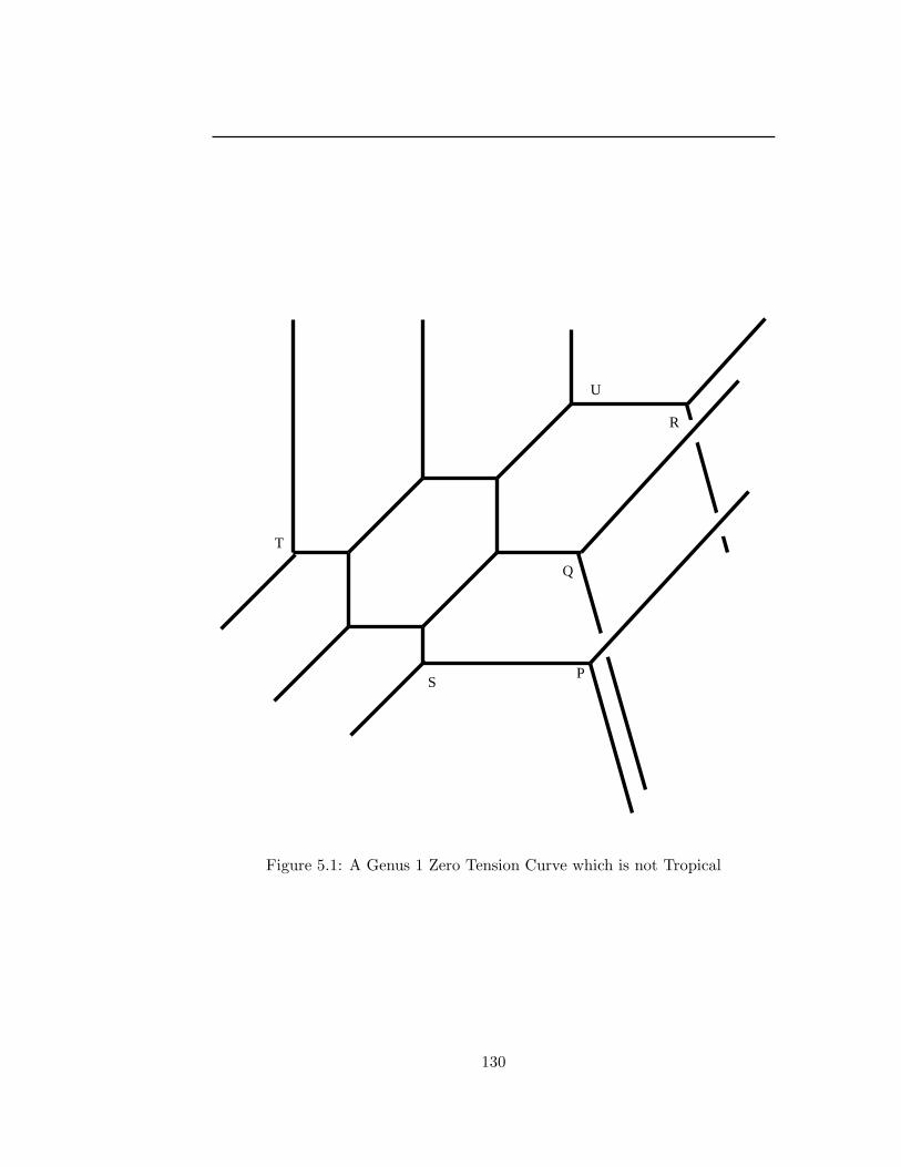
P
U
T
S
R
Q
Figure 5.1: A Genus 1 Zero Tension Curve which is not Tropical
130
always a tropical curve. In this section, we will prove that conjecture completely
when κ has characteristic zero, we will need some hypotheses on the characteristic
of κ when our curve has genus greater than 2.
Theorem 5.0.4. If κ has characteristic zero, then every ordinary zero-tension
curve is the tropicalization of a curve of corresponding genus and degree. Every
ordinary zero-tension curve of genus 0 or 1 is the tropicalization of a curve of
corresponding genus and degree. If Γ is an ordinary zero tension curve and κ has
characteristic p then Γ is the tropicalization of a curve of corresponding genus
and degree assuming that the matrix Slope(Γ, ι, wt) defined in Section 5.1 has full
rank modulo p.
These characteristic issues are frustrating. I do not have any examples
where an ordinary zero tension curve in characteristic p is not achievable as the
tropicalization of a curve and very much suspect that none exist. The matrix
Slope(Γ, ι, wt) referred to in the above theorem is a matrix of integers which has
full rank if and only if the zero tension curve is ordinary. All of the dependency
on characteristic is bound up in Lemma 5.7.1, and we will discuss it more fully
at that point.
Mikhalkin has announced a proof of the above conjecture by means of
Floer cohomology, which is yet to appear. Our methods will be very different
from Mikhlkain’s; we use nonarchimedean analysis and uniformizations of curves.
Note that our terminology differs from that of Mikhalkin in [24], who
131

COMBINATORICS OF ZERO TENSION CURVES
would call something a tropical/parameterized tropical curve if it was a com-
binatorial object that looked like one of our objects. We reserve the adjective
“tropical” to refer to graphs that actually occur as tropicalizations and will refer
to combinatorial things that look like tropical curves as “zero-tension”.
Finally, we should note that our work bears some interesting resem-
blances to that of [28] and the sequels to that paper. Morgan and Shalen com-
pactify Teichmuller space, which they think of as the space of two dimensional
representations of the free group, by using amoebas and Bergman’s notion of a
logarithmic limit set. This latter is the same as the tropicalization. Teichmuller
space is also closely related to the moduli space of curves, a connection which
Morgan and Shalen mention but do not emphasize as they are more concerned
with applications to three dimensional hyperbolic manifolds. The main compu-
tations in this section deal with studying maps of curves to toric varieties, which
Morgan and Shalen do not pursue.
5.1 Combinatorics of Zero Tension Curves
Let Γ be a finite graph. Let Γfin be the subgraph of Γ consisting of the edges
neither of whose endpoints has degree 1; we will call an edge which has an end
point of degree 1 an infinite edge and an edge which does not have such an
endpoint a finite edge. Let w : Edge(Γ) → Z 0 be a function assigning a positive
integral weight to each edge. Let ι : Γ \ vertices of degree one → Rn be
132
COMBINATORICS OF ZERO TENSION CURVES
a continuous map under which each unbounded edge of Γ is taken to a semi-
infinite ray, each finite edge is taken to a line segment of finite (nonzero) length
and each of these rays and line segments has rational slope. We will use abuse
notation by writing ι : Γ → Rn. For e an edge and v one of its endpoints, let
σv(e) be the primitive lattice vector pointing in the direction of ι(e) away from
ι(v) and let σv(e) = w(e)σv(e). σv(e) is the important definition, σv(e) will only
occur rarely. Notice that, if e has endpoints v1 and v2, then σv1(e) = −σv2(e).
We call (Γ, ι, w) a zero tension curve if, at every vertex v not of degree
1, we have∑
e3v σv(e) = 0. We sometimes will abuse notation by referring to Γ
as the zero tension curve, saying, for example, “If a zero tension curve is a tree...”
We saw in Section 2.5 that, if X ⊂ (K∗)n is a curve then TropX naturally has
the structure of ι(Γ) for a zero tension curve (Γ, ι, w). The goal of this section
is to prove some combinatorial results about zero tension curves. We assume for
convenience that Γ is connected.
Suppose that if v is a vertex of Γ of degree 2 with edges e1 and e2 coming
out of it connected to vertices u1 and u2. Then σv(e1) = −σv(e2). This forces
ι(e1) and ι(e2) to be parallel and point in opposite directions away from ι(v) (since
w(e1) and w(e2) > 0) so σv(e1) = −σv(e2) and w(e1) = w(e2). Let Γ′ be the
graph obtained by deleting v, e1 and e2 and inserting a single edge e0 between u1
and u2. Define the weight function w′ on Γ′ by having w′(e) = w(e) for every edge
w other than e0 and w′(e0) = w(e1) = w(e2). Define ι′ : Γ′ → Rn∪∞ by having
133
COMBINATORICS OF ZERO TENSION CURVES
ι′ coincide with ι on the edges other than e0 and having ι′(e0) = ι(e1) ∪ ι(e2).
Thus, we have replaced (Γ, ι, w) with a new zero tension curve (Γ′, ι′, w′) which
has one fewer vertex. Continuing in this manner, we will always eventually arrive
at a zero tension curve with no vertices of degree 2. Since most of our results
will be unaffected by this reduction procedure, we will often restrict to the case
of curves that have no vertices of degree 2, which we term non-bivalent. An
especially important case is the case where each vertex is either of degree 3 or 1,
which we term trivalent.
We define the degree of a zero tension curve to be the unordered list of
vectors σv(e) where v runs over the degree 1 vertices. We define the genus of
a zero tension curve to be the first Betti number of Γ. The main result of this
section is
Theorem 5.1.1. The collection of non-bivalent zero tension curves of given
genus and degree in Rn, modulo reparameterization, naturally has the structure
of a finite union of rational polyhedral cones (in some RN ).
We will use the variable x to denote the number of infinite edges of Γ.
Lemma 5.1.2. Assume Γ is non-bivalent. Let V denote the number of non-
degree 1 vertices of Γ and E the number of finite edges. Then V ≤ x + 2(g − 1)
and E ≤ x+ 3(g− 1), with equality in each case if and only if Γ is trivalent.
Proof. By counting the number of pairs (vertex, edge containing vertex) in two
ways, we get 2(E+ x) ≥ 3V + x, with equality if and only if Γ is trivalent. Also,
134
COMBINATORICS OF ZERO TENSION CURVES
(E + x) − (V + x) = g − 1 so E = V + g − 1 and V = E − g + 1. Substituting
these into the previous inequality gives the desired results.
Define the combinatorial type of a zero tension curve to be underlying
abstract graph Γ and the data of the vectors σv(e).
Proposition 5.1.3. The set of zero tension curves of given combinatorial type
has the structure of the relative interior of a cone. Using the notations V and
E for the number of finite edges and finite vertices, this cone (if nonempty) has
dimension at least E − n(g − 1).
Proof. This is fairly clear. All that remains to specify a zero tension curve once its
combinatorial type is known is to give the coordinate of one vertex (n parameters)
and the lengths of the finite edges (E parameters, each required to be positive.)
Not every collection of edge lengths is legitimate however: all of the cycles must
close up. It is enough to check this for a collection of g cycles forming a homology
basis of Γ, we get n equations for each cycle. Thus, we are looking at a slice of
an open quadrant of Rn+E by a plane of codimension at most ng, so it is a cone
of dimension at least E − n(g − 1).
Remark: When Γ is trivalent, this bound is x− (n− 3)(g − 1) by the
above lemma. If we are considering degree d curves in three space, so x = 4d,
then this quantity is 4d which is a standard lower bound for the dimension of the
Hilbert scheme of degree d, genus g curves in projective n space. According to
135
COMBINATORICS OF ZERO TENSION CURVES
Hartshorne, the first proof of this bound may be in [16], lemma 5, although the
result is far older.
We define a combinatorial type to be ordinary if this cone has dimension
E − n(g− 1) and superabundant otherwise. Let us note explicitly what it means
to be ordinary: choose a basis γ1, . . . , γg for H1(Γ). We define a gn×E matrix
Slope(Γ, ι, wt) whose columns are indexed by the edges of Γand whose rows are
indexed by ordered pairs (i, γj) with 1 ≤ i ≤ n, 1 ≤ j ≤ g. The ((i, γj), e) entry
of Slope(Γ, ι, wt) is σv1(e)(e)j times the (signed) number of times that e appears
in γi. Clearly, Slope(Γ, ι, wt) depends only on the combinatorial type of (Γ, ι, wt).
(Γ, ι, wt) is ordinary if and only if Slope(Γ, ι, wt) has full rank.
Remark: Mikhalkin, in [25], seems to suggest that every zero tension
curve can be perturbed to a trivalent zero tension curve. This is easy to prove
when the curve is ordinary; more specifically, we have:
Proposition 5.1.4. Let (Γ, ι, w) be a zero tension curve and let v be a vertex of
Γ of degree 4 or greater. Form a new graph Γ′ by replacing v with two vertices
v1 and v2, connected to each other by an edge and such that every neighbor of v
is connected to either v1 or v2 and each of v1 and v2 has degree at least 3. It is
possible to find a family ιt of embeddings of Γ′ into Rn as a zero tension curve
such that: each edge of ιt(Γ′) other than ι((v1, v2)) is parallel to the corresponding
edge of ι(Γ), ιt((v1, v2)) shrinks down to ι(v) as t→ 0 and, for every other edge
e, ιt(e) → ι(e) as t→ 0.
136
COMBINATORICS OF ZERO TENSION CURVES
Proof. Define a third graph Γ′′ by removing the edge (v1, v2) from Γ′ and adding
an unbounded edge at each of v1 and v2. There are two cases, based on whether
or not Γ′′ is connected. If Γ′′ is not connected, then we can simply make a family
of embeddings of Γ′ as in the hypotheses of the theorem by fixing the location of
ι(v1) at v, keeping every edge other than (v1, v2) of constant length and giving
the edge (v1, v2) length t and the slope forced by the zero tension condition.
We now turn to the case where Γ′′ is connected. We consider the family
of embeddings of Γ′′ of the following combinatorial type: every edge of Γ′′ has
the same slope as the corresponding edge in Γ except for the two unbounded
edges which have the slopes forced by the zero tension condition. Now, Γ′′ has
exactly as many finite edges as Γ but is of one lesser genus. We can choose
our basis of cycles for Γ so that only one of them, say c, when pulled back to
Γ′, goes along (v1, v2). The equations which describe the cones of embeddings
of Γ′′ of the specified combinatorial type are the same as those for Γ′′ plus the
equation that says the cycle c closes. We can thus think of the embeddings of Γ
as embeddings ι′′ of Γ in which the cycle c closes or, equivalently, ι′′(v1) = ι′′(v2).
Since the combinatorial type of (Γ, ι, w) is ordinary, all of the equations cutting
out the cone of embeddings are non-redundant and so the possible directions of
ι′′(v1) − ι′′(v2) must span Rn. In particular, we can find embeddings ι′′ of Γ′′
where ι′′(v1) approaches ι′′(v2) while ι′′(v1)− ι′′(v2) has the slope which the edge
(v1, v2) of Γ′ is forced to have by the zero tension condition. Then deleting the
137

COMBINATORICS OF ZERO TENSION CURVES
unbounded rays and drawing back in (v1, v2) gives a sequences of embeddings of
Γ′ as desired.
Applying this result over and over again, every ordinary curve can be
written as a degeneration of a trivalent curve. In the superabundant case, one
often can not choose how to split the edge incident on a vertex of degree ≥ 4 and
sometimes can not split one vertex without splitting another vertex elsewhere.
Nonetheless, it seems like it may always be true that every zero tension curve
can be written as the limit of trivalent zero tension curves.
So the set of nonbivalent zero tension curves of given degree and genus is
a union of cones, one for each combinatorial type, and we must simply show that
there are finitely many combinatorial types of zero tension curve of each genus
and degree. First note that there are only finitely many nonbivalent graphes with
x degree one vertices and first Betti number g. (Proof: they are all subgraphs of
the complete graph on (x+2g− 2)+x vertices.) Thus, it is enough to prove, for
a fixed graph Γ and a choice of degree, that there are only finitely many choices
for the slopes σv(e). Explicitly, a choice of degree means specifying the slope
σv(e) for each infinite edge e of Γ. We will prove:
Proposition 5.1.5. For each i between 1 and n, there are only finitely many
possible choices for the integer valued function (σv(e))i.
Proof. Fix an orientation of the graph Γ, so that each edge e has a chosen ordering
(v1(e), v2(e)) of its endpoints. Let C1 be the free abelian group on the edges of
138
COMBINATORICS OF ZERO TENSION CURVES
Γ.
Now, suppose we are given an integer valued function s(e) on the finite
edges of Γ and a positive real valued function ` on the finite edges. Suppose
there is a zero tension curve with underlying graph Γ, with s(e) = (σv1(e)(e))i =
−(σv2(e)(e)) and with `(e)σv1(e)(e) parallel to and the same length as ι(e). Con-
sider the element S =∑
e∈Γfin s(e)e of C1. Let T be the analogous sum over the
infinite edges; note that T is fixed by our knowledge of the degree. Letting ∂
denote the map C1 → C0 sending e 7→ v1(e) − v2(e), the zero tension condition
states that ∂(S + T ) = 0. Thus, ∂S is determined and we see that the different
possible values for S differ by members of Ker ∂ = H1(Γ).
On the other hand, the assumption that the cycles of Γ close up tells
us that S is in the orthogonal complement of H1(Γ) with respect to the inner
product <,>` under which the finite edges of Γ are orthogonal and have norm
< e, e >`= `(e). We are therefore reduced to proving the following proposition,
with RN = C1 ⊗ R, H = H1(Γ)⊗ R and v0 = S0.
Lemma 5.1.6. Let H be a sub-vector space of RN and let v0 ∈ RN . Let S denote
the set of points v ∈ RN such that (1) v ∈ v0 + H and (2) v is orthogonal to
H for some inner product which is diagonal and positive definite in the standard
basis of RN . Then S is bounded. More precisely, form a hyperplane arrangement
A in v0 +H by intersecting v0 +H with the coordinate hyperplanes of RN . Then
S is the interior of the union of the bounded regions of A. In particular, this set
139
COMBINATORICS OF ZERO TENSION CURVES
contains finitely many lattice points.
Proof. First, suppose that v1 is not in the interior of the bounded part of A.
Then there is a w ∈ H \ 0 such that v1 + tw lies in the same region of A for
all t > 0. For every coordinate i for which wi is nonzero, wi and (v1)i must
have the same sign. But then < v1, w >` is entirely a sum of positive terms and
< v1, w >`> 0, contradicting that v1 ∈ H⊥.
Conversely, suppose that v1 is in the interior of of the bounded part of
A. Then there is no w ∈ H \ 0 such that v + tw lies in the same component
of A for all t > 0. Reversing the above, that means that there is no w ∈ H such
that wi and (v1)i have the same sign whenever wi 6= 0. By linear programming
duality (see, for example, proposition 6.8 in [51]), this implies that H⊥ contain
an element with the same sign pattern as v1, say v2. Set αi = (v2)i/(v1)i with αi
an arbitrary positive real when (v2)i = (v1)i. Set `′i = αi`i. Then v1 is orthogonal
to H with respect ot <,>`′ .
When g = 0, this proof shows that there is a unique combinatorial type
given the underlying graph Γ and its degree. When g = 1, Γ has a unique loop v1,
. . . , vr. The above proof shows that σv(e) is uniquely determined for e not in the
loop. Moreover, for each vi, let di be the sum of σvi(e) summed over e 3 vi where
e is not in the loop, then the possible combinatorial structure are in bijection
with the lattice points in the interior of the convex hull of the di. When g ≥ 2,
140
THE BRUHAT-TITS TREE AND CROSS-RATIOS
it is easy enough to compute the bounded regions for each coordinate 1 ≤ i ≤ n,
but I don’t know a simple way to figure out when two solutions coming from
lattice points from different i can arise from the same `.
5.2 The Bruhat-Tits Tree and Cross-Ratios
In this section we review some standard constructions. A good reference for these
results with a view towards the sort of applications we will be making is Chapter
2 of [28]. For simplicity, we will assume that v : K∗ → R is surjective.
We denote by BT(K) the set of R-submodules of K2 which are iso-
morphic to R2, modulo K∗-scaling. We write M for the equivalence class of a
module M . We equip BT(K) with the metric where d(M1,M2) is the infimum
of all ε such that there exists an α with M1 ⊇ tαM2 ⊇ tεM1; this is easily seen
to be independent of the choice of representatives M1 and M2. BT(K) is called
the Bruhat-Tits tree of K.
If we made the analogous construction working with the field of power
series of integral exponents, we could equip BT(K) with the structure of the
vertices of a tree so that distance was the graph theoretic distance. Instead,
BT(K) is what is called an R-tree (see [28]). The following proposition lists the
“tree-like” properties of BT(K).
Proposition 5.2.1. If M1 and M2 ∈ BT(K) with d(M1,M2) = d then there
is a unique distance preserving map φ : [0, d] → BT(K) with φ(0) = M1 and
141
THE BRUHAT-TITS TREE AND CROSS-RATIOS
φ(d) = M2. We will call the image of φ the path from M1 to M2 and denote it
by [M1,M2]. If M1, . . . , Mn ⊂ BT(K) then ∪i6=j [M1,M2] is a tree.
It is easy to give an explicit description of φ: if M1 ⊇ M2 ⊇ tdM1
then φ(e) = teM1 +M2. Suppose now that (x1 : y1) and (x2 : y2) are distinct
members of P1(K). Then we can similarly define a map φ : R → BT(K) by
φ(e) = R(x1, y1) + teR(x2, y2). We will call the image of this φ the path from
(x1 : y1) to (x2 : y2) and denote it [(x1 : y1), (x2 : y2)]. Similarly, if M ∈ BT(K)
and (x1 : y1) ∈ P1(K), we can define a semi-infinite path from (x1 : y1) to M
denoted [(x : y),M ].
If Z is a subset of BT(K) ∪ P1(K), we denote by [Z] the subspace
∪z,z′∈Z [z, z′] ⊂ BT(K). For simplicity, assume that |Z| ≥ 3. If Z is finite, [Z]
is a tree with a semi-infinite ray for each member of Z ∩ P1(K). We will say
that this ray has its end at the corresponding member of Z ∩ P1(K). We will
abbreviate [x1, . . . , zn] as [z1, . . . , zn].
The particular case where Z is a four element subset of P1(K) is of
particular importance. Let w, x, y, z ⊂ P1(K) = K∪∞. We define the cross
ratio c(w, x : y, z) by
c(w, x : y, z) =(w− y)(x− z)
(w− z)(x− y).
Note that c(w, x : y, z) = c(x, w : z, y) = c(y, z : w, x) = c(z, y : x, w).
Proposition 5.2.2. [w, x, y, z] is a tree with 4 semi-infinite rays and either 1 or
2 internal vertices.
142
THE BRUHAT-TITS TREE AND CROSS-RATIOS
If [w, x, y, z] has two internal vertices, let d be the length of the internal
edge and suppose that the rays ending at w and x lie on one side of that edge
and the rays through y and z on the other. Then v(c(w, x : y, z)) = 0, v(c(w, y :
x, z)) = d and v(c(w, y : z, x)) = −d. The first statement can be strengthened to
say that v(c(w, x : y, z) − 1) = d. (All other permutations of w, x, y, z can be
deduced from this).
If [w, x, y, z] has only one internal vertex then v(c(w, x : y, z)) = 0
and the same holds for all permutations of w, x, y, z.
This proposition can be remembered as saying “v(c(w, x : y, z)) is the
signed length of [w, x]∩ [y, z]” where the sign tells us whether the two paths run
in the same direction or the opposite direction along their intersection.
Proof. Due to the invariance of the definition of BT(K), the group GL2(K) acts
on it and, since we only consider submodules of K2 up to K∗, GL2(K) acts
through its quotient PGL2(K). This action is compatible with the standard
action of PGL2(K) on P1(K) = K ∪ ∞. It is well known that c is PGL2(K)
invariant. So the whole theorem is invariant under PGL2(K) and we may use this
action to take w, x and y to 0, 1 and ∞. Our hypothesis in the second paragraph
is that [0, 1,∞, z] is a tree with 0 and 1 on one side of a finite edge of length d and
z and ∞ on the other. It is easy to check that this is equivalent to requiring that
v(z) = −d < 0. Then c(0, 1 : ∞, z) = 1− 1/z which does indeed have valuation 0
and c(0, 1 : ∞, z) − 1 = −1/z does indeed have valuation d. c(0,∞ : 1, z) = 1/z
143

TROPICAL GENUS ZERO CURVES
which has valuation d and c(0,∞ : z, 1) = z which has valuation −d. In the
second paragraph, the assumption that the tree has no finite edge implies that
v(z) = v(z − 1) = 0 and the argument then continues as before.
5.3 Tropical Genus Zero Curves
The aim of this section is to prove Theorem 5.0.4 in the case where Γ is a tree
so we want X to have genus 0. This result will appear in a future publication of
Mikhalkin; it also appears with many results on incidence conditions in [30]. Our
method of proof is not only far more explicit than these, but it will be a good
warm up for the case of higher genus curves. Note that this will generalize the
characterization of tropicalizations of lines in Chapter 3. Let (Γ, ι, w) be a zero
tension curve with Γ a tree. Put a metric on Γ such that the unbounded edges
have infinite length and the length ` of a finite edge e is chosen such that ι(e) is
a displacement of `σv(e).
Proposition 5.3.1. Let T be a metric tree with finitely many vertices such that
each degree 1 vertex of T is at the end of an infinite ray. Then there is a Z ⊂
P1(K) such that [Z] is isometric to [T ]. If we permit some of the degree 1 vertices
of T to be at the end of finite length edges then we can still embed T as a subtree
of BT(K).
Proof. First, we consider the case where each degree 1 vertex of T is at the end
of an infinite ray.
144
TROPICAL GENUS ZERO CURVES
Our proof is by induction on the number of finite edges of T . If T has
l leaves and no finite edges then T is isometric to [z1, . . . , zl] for z1, . . . , zl any
l elements of K∗ with valuation 0 and distinct images in κ∗.
Now, let e be a finite edge of T of length d joining vertices v1 and v2.
Remove e from T , separating T into two trees T1 and T2. Define trees T ′s, where
s = 1, 2, by adding an unbounded edge to Ts at vs. By induction, we can find
subsets Z1 and Z2 ⊂ P1(K) with [Zs] isometric to T ′s. Let zs ∈ Zs be the element
of Zs at the end of the new ray added to Ts. Without loss of generality, we may
assume that z1 = 0 and z2 = ∞. Then the point of Ts corresponding to vs lies
somewhere on [0,∞]. By multiplying Z1 and Z2 by elements of K∗, we may
assume that these points lie distance d apart with v1 closer to 0 than v2 is to 0.
Then T is isometric to [Z1 ∪ Z2].
Finally, if not each degree 1 vertex of T is at the end of an infinite
ray then we can embed T into a tree T ′ which does have this property, find an
isometric embedding of T ′ in BT(K) by the above and then T will be embedded
as a subtree of T ′.
Let Z ⊂ P1(K) be such that [Z] is isometric to Γ. We define multisets
Z+1 , . . . , Z+
n , Z−1 , . . . , Z−
n as follows: All of the elements of Z±,i lie in Z. Let
z ∈ Z correspond to the end of an infinite ray e of Γ. Suppose that σz(e) =
(s1, . . . , sn). Then z ∈ Z±,i if and only if ±si < 0. In this case, |si| is the number
of times that z occurs in Z±,i. Define a rational map φ : P1(K) → Kn by the
145
TROPICAL GENUS ZERO CURVES
formula
φ(u) = (φ1(u), . . . , φn(u)) =
(∏
z∈Z+1(u− z)
∏
z∈Z−
1(u− z)
, . . . ,
∏
z∈Z+n(u− z)
∏
z∈Z−
n(u− z)
)
.
Here u is a coordinate on P1(K), thought of as K ∪ ∞.
Theorem 5.3.2. Tropφ(P1(K)) is a translation of ι(Γ).
Clearly, φ(P1(K)) is a genus zero curve of the appropriate degree. From
now until the end of the proof, we identify [Z] with Γ so that we can write
ι : [Z] → Rn.
Proof. Let u ∈ P1(K) \ Z. Then [Z] is a tree and [Z ∪ u] is a tree with one
additional end. Let b(u) ∈ [Z] be the point at which that end is attached. We
claim that, up to a translation, v(φ(u)) is ι(b(u)). In other words, if u1 and u2
are distinct members of u ∈ P1(K) \ Z, we must show that for each i between 1
and n we have
v(φi(u1)) − v(φi(u2)) = ι(b(u1))i − ι(b(u2))i.
It is enough to show this in the case where b(u1) and b(u2) lie in the
same edge e of [Z]. We will fix one coordinate i to pay attention to, so i will
not appear in our notation. Let Z+i = z+
1 , . . . , z+r and Z−
i = z−1 , . . . , z−r . We
may find constants 1 ≤ s+, s− ≤ n and order the z±j such that z±j is on the b(u1)
side of e for 1 ≤ j ≤ s± and on the b(u2) side of e for s± + 1 ≤ j ≤ r. Let d be
the distance from b(u1) to b(u2).
146
TROPICAL GENUS ZERO CURVES
We have
v(φi(u1)) − v(φi(u2)) = v
(
φi(u1)
φi(u2)
)
= v
(
∏rj=1(u1 − zj)
+/∏r
j=1(u1 − zj)−)
(
∏rj=1(u2 − zj)+/
∏rj=1(u2 − zj)−
)
= v
r∏
j=1
c(u1, u2 : z+j , z
−j )
=
r∑
j=1
v(c(u1, u2 : z+j , z
−j )) = d(s+ − s−).
The last equality is by applying Proposition 5.2.2 to each term.
By the zero tension condition, si(e) = s+ − s− (recall that the slope of
ι(e) is (s1(e), . . . , sn(e)) .) So ι(b(u1))i − ι(b(u2))i is also d(s+ − s−).
We pause for two examples.
Example 5.3.3. Consider the tree in R3 with a finite edge running from (0, 0, 0)
to (1, 1, 1) , infinite edges leaving (1, 1, 1) in directions (1, 0, 0) and (0, 1, 1) and
edges departing (0, 0, 0) in directions (0,−1, 0) and (−1, 0,−1). Then [0, t, 1, t−1]
is isometric to Γ, with 0, t,1 and t−1 respectively corresponding to the endpoints
of the above infinite rays. We have
Z+,1 = 0 Z+,2 = t Z+,3 = t
Z−,1 = t−1 Z−,2 = 1 Z−,3 = t−1
Thus, the map φ is given by
u 7→
(
u
u− t−1,u− t
u,u− t
u − t−1
)
.
147
TROPICAL GENUS ONE CURVES
The image of this map is a genus 0 curve X with TropX equal to the given tree.
Example 5.3.4. This time we choose a tree with no internal edges but complci-
ated slopes. Consider the tree T in R3 with no internal edges and four unbounded
rays of slope (1, 2, 3), (5,−3, 4), (−7, 1,−2), (1, 0,−5). Assuming that κ has char-
acteristic 0, the tree [1, 2, 3, 4]⊂ BT(K) is isometric to T . Our multisets Z±i are
Z+,1 = 1, 2, 2, 2, 2, 2, 4 Z+,2 = 1, 1, 3 Z+,3 = 1, 1, 1, 2, 2, 2, 2
Z−,1 = 3, 3, 3, 3, 3, 3, 3 Z−,2 = 2, 2, 2 Z−,3 = 3, 3, 4, 4, 4, 4, 4
For example, there are 5 occurences of the number 4 in Z−,3 because ray number
4 of out tree has slope −5 in the x3 direction.
Our map φ is given by
u 7→
(
(u− 1)(u− 2)5(u− 4)
(u− 3)7,(u− 1)2(u− 3)
(u− 2)3,(u− 1)3(u− 2)4
(u− 3)2(u− 4)5
)
.
Once again, the image of φ is a genus zero curve whose tropicalization
is the given tree.
5.4 Tropical Genus One Curves
Let (Γ, ι, w) be a zero tension curve where Γ is connected with first Betti number
1. This means that Γ has a unique cycle, let e1, . . . , er be the edges of this cycle
and let σi be σ(ei).
Our aim in this section is to prove
148
TROPICAL GENUS ONE CURVES
Theorem 5.4.1. If (Γ, ι, w) is ordinary then there is a genus one curve X ∈
(K∗)n with TropX = ι(Γ)
Let us make the condition of the theorem more explicit:
Proposition 5.4.2. (Γ, ι, w) is ordinary if and only if the σi span Rn.
Proof. Consider the equation∑
`iσi = 0 where `i ∈ R. By definition, (Γ, , ι, w)
is ordinary if this equation has solution space of codimension n in Rr. In other
words, the kernel of the map taking Rr → Rn via (`1, . . . , `r) 7→∑
`iσi = 0 must
be (r − n)-dimensional or, in other words, the map must be surjective. This
precisely says that the σi span Rn.
We use Tate’s nonarchimedean uniformizations of elliptic curves. A
good reference for this subject is chapter V of [34]. Let q ∈ K∗ with v(q) > 0.
Tate constructs an elliptic curve E over K with a bijection p from K∗/qZ to
E(K). For z+, z− ∈ K∗, define
φz+ ,z−(u) =
0∏
i=−∞
(
u/z+ − qi
u/z− − qi
) ∞∏
i=1
(
u− qiz+
u− qiz−
)
This product is convergent in the nonarchimedean topology on K for all u ∈
K∗ \ qZ · (z+, z−) and φ(qu) = (z+/z−)φ(u). (Remember that limn→∞ qn =
0 because v(q) > 0.) Thus, if Z+ = z+1 , . . . , z
+k and Z− = z−1 , . . . , z
−k
are finite multisubsets of K∗ with the same cardinality and∏k
i=1(z+i /z
−i ) =
1 then φZ+,Z−(u) :=∏k
i=1 φz+i ,z−i
(u) is a well defined function on (K∗/qZ) \
(
⋃∞j=∞ qj · z+
1 , . . . , z+k , z
−1 , . . . , z
−k )
. Thought of as a function on E(K) with
149
TROPICAL GENUS ONE CURVES
the appropriate points removed, Tate proves that this is a rational function with
zeroes at the points p(z+i ) and poles at p(z−i ), where p is the projectionK∗/qZ →
E(K).
Let f1, . . . , fm be the set of unbounded rays of Γ and vi their end-
points. Let dj =∑m
i=1 max(σvi(fi)j , 0) = −
∑mi=1 min(σvi
(fi)j , 0). The equality
is because, by the zero tension condition,∑m
i=1 σvi(fi) = 0. Let Z+
1 , . . . , Z+m,
Z−1 , . . . , Z−
m be multisubsets of (K∗)n with |Z+i | = |Z−
i | = di. Let `i be the
length of ei and let ` =∑
`i. Choose q ∈ K∗ with v(q) = `.
Let ג be the subtree of BT(K) spanned by⋃∞
i=∞ qi(
⋃nj=1
(
Z+j ∪ Z−
j
))
.
Let ג be the quotient of ג under the translation by qZ. ,ג) pronounced “gimmel”,
is the Hebrew letter analogous to G and Γ. We need to reserve G for a certain
group that will appear in the next section.)
Choose an ordering (z±,1i , . . . , z±,di
i ) of each of the Z±i . Consider all of
the paths [z−,ki , z+,k
i ] for 1 ≤ k ≤ di and take their images down in ;ג call this
collection Pi. For an edge e of ג with endpoint v, by “the number of signed
paths of Pi running along e away from v”, we mean to count each path with sign
according to whether it runs towards or away from v along e and multiplicity
counting how many times it passes through e.
Proposition 5.4.3. It is possible to choose Z±i and q such that
1. There is an isometry ψ : ג∼→ Γ.
2. If e is an edge of ג with end point v then the ith component of σv(ψ(e)) is
150
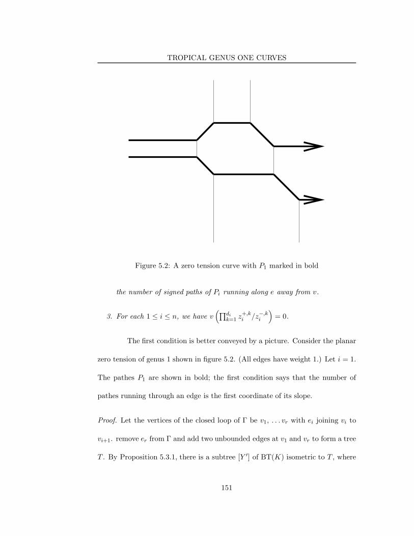
TROPICAL GENUS ONE CURVES
Figure 5.2: A zero tension curve with P1 marked in bold
the number of signed paths of Pi running along e away from v.
3. For each 1 ≤ i ≤ n, we have v(
∏di
k=1 z+,ki /z−,k
i
)
= 0.
The first condition is better conveyed by a picture. Consider the planar
zero tension of genus 1 shown in figure 5.2. (All edges have weight 1.) Let i = 1.
The pathes P1 are shown in bold; the first condition says that the number of
pathes running through an edge is the first coordinate of its slope.
Proof. Let the vertices of the closed loop of Γ be v1, . . . vr with ei joining vi to
vi+1. remove er from Γ and add two unbounded edges at v1 and vr to form a tree
T . By Proposition 5.3.1, there is a subtree [Y ′] of BT(K) isometric to T , where
151
TROPICAL GENUS ONE CURVES
Y ′ is a finite subset of P1(K). By an automorphism of P1(K), we may arrange
that the ends of the new edges added at v1 and vr are at 0 and ∞.
Let Y = Y ′ \ 0,∞. We define the multisets Z±,i as follows: every
element of Z±,i is an element of Y . Let y ∈ Y correspond to the infinite edge e
of Γ, then y ∈ Z±,i if and only if ±σy(e)i < 0 and the number of times that y
occurs is |σy(e)i|.
Choose q with v(q) = `. Let σvr (er) = (s1, . . . , sn). Choose Z±i as
follows: We take Z−i = Y −
i . Z+i is the same as Y +
i except that we multiply y+,1i
by qsi . We claim that the proposition holds for this Z±i and this q. It is clear
that Γ and ג are isomorphic as graphs, we must check that the corresponding
edges have the same lengths to prove claim (1). By constructing [Y ′] isometric to
T , this is automatic for every edge except the ones corresponding to er. By our
choice to make v(q) = `, multiplication by q shifts ג by ` along the path [0,∞] so
the cycle in ג has length `. The cycle in ι(Γ) also has length ` and all the other
edges are the right length, so (1) follows.
For (2), we break into cases depending on the location of the edge e.
First, suppose that e is not in the closed loop of .ג Then removing e from ג
disconnects e into a tree and a graph with a loop, we may assume that v is in
the end that is a tree. Then the number of signed paths of Pi running along e
away from v is simply the number of those paths ending in the tree minus the
number starting in the tree. By construction, this is the sum of the i components
152
TROPICAL GENUS ONE CURVES
of the directions of the corresponding infinite rays in ι(Γ). By the zero tension
condition, these two numbers match.
Next, suppose that e = er and v = vr. The only path in Pi crossing er
is the image of [y−,1i , qsiy+,1
i ]. This path runs along er away from v si times so
(2) holds in this case.
Finally, let tv(e)i denote the number of times a path in Pi runs along
e away from v. Since every path that enters v must leave it,∑
e3v tv(e)i = 0.
In other words, the vectors (tv(e)1, . . . , tv(e)n) obey the zero tension condition.
The σv(e), of course, also obey the zero tension condition. But once we have
determined tv(e) on all edges except the chain e1, . . . , er−1, the zero tension
condition forces these remaining edges to be correct as well.
We now turn to (3). v(z+,ki /z
−,ki ) is the length of the overlap between
the paths [z+,ki , z−,k
i ] and [0,∞]. Thus v(
∏di
k=1 z+,ki /z−,k
i
)
=∑di
k=1 v(z+,ki /z−,k
i )
is the sum over all k of the length of this overlap. Pushing the paths [z+,ki , z−,k
i ]
and [0,∞] down to ,ג our problem is to sum over the paths of Pi the length of
the signed overlap of Pi with the closed loop of .ג Breaking up our sum over the
edges of the closed loop and using property (3), this is∑
`jσvj(ej)i where the
subscript i means to take the i component. But∑
j `jσvj(ej) = 0 because the
loop closes, so we are done.
Choose q and Z±i as in the above proposition. If we knew that for each
i we had∏
z+∈Z+iz+ =
∏
z−∈Z−
iz− then we would have an embedding of the
153
TROPICAL GENUS ONE CURVES
elliptic curve K∗/qZ in (K∗)n via φ : u 7→ (φZ+1 ,Z−
1(u), . . . , φZ+
n ,Z−
n(u)).
Proposition 5.4.4. If we have∏
z+∈Z+iz+ =
∏
z−∈Z−
iz−, define the genus one
curve X ⊂ (K∗)n by the above embedding. Then TropX is a translate of ι(Γ).
(So by translatingX by an element of (K∗)n we can arrange that TropX = ι(Γ).)
Proof. Let u1 and u2 ∈ K∗ \⋃∞
i=∞ qi(
⋃nj=1
(
Z+j ∪ Z−
j
))
. Consider the tree
[us∪⋃∞
i=∞ qi(
⋃nj=1
(
Z+j ∪ Z−
j
))
] ⊂ BT(K), where s = 1, 2. This tree contains
ג and one additional unbounded edge, let b(ui) be the point of ג at which the
new unbounded edge is attached. We claim that
φ(u2) − φ(u1) = ι(ψ(π(b(u2))))− ι(ψ(π(b(u1))))
where π is the projection ג → ג and ψ is the identification ג → Γ. As u2 varies
over K∗ \⋃∞
i=∞ qi(
⋃nj=1
(
Z+i ∪ Z−
i
)
)
, the point b(u2) varies over ג so φ(u2)
sweeps out a translate of ι(ψ(ג)) = ι(Γ), as desired.
We now check the claim. It is enough to consider the case where b(u1)
and b(u2) lie on the same edge e of ,ג say at distance d apart. We can check
the claim coordinate by coordinate; we focus on the i coordinate, so we must
compute v(φZ+,i ,Z−,i(u2)) − v(φZ+,i ,Z−,i(u1)). We have
φZ+,i ,Z−,i(u2)
φZ+,i ,Z−,i(u1)=
di∏
k=1
0∏
j=−∞
(u2/z+,ik − qj)(u1/z
−,ik − qj)
(u2/z−,ik − qj)(u1/z
+,ik − qj)
∞∏
j=1
(u2 − qjz+,ik )(u1 − qjz−,i
k )
(u2 − qjz−,ik )(u1 − qjz+,i
k )
154
TROPICAL GENUS ONE CURVES
=
di∏
k=1
∞∏
j=−∞
(u2 − qjz+,ik )(u1 − qjz−,i
k )
(u2 − qjz−,ik )(u1 − qjz+,i
k )
=
di∏
k=1
∞∏
j=−∞
c(u2, u1 : qjzi,+k , qjzi,−
k ).
(In the nonarchimedean topology all convergent products and sums are absolutely
convergent, so we may rearrange freely.) So
v(φZ+i ,Z−,i(u2)) − v(φZ+
i ,Z−,i(u1)) =
di∑
k=1
∞∑
j=−∞
v(c(u2, u1 : qjzi,+k , qjzi,−
k )).
By Proposition 5.2.2, each summand is the signed length of the overlap
of [u2, u2] and [qjzi,+k , qjzi,−
k ]. Now, [qjzi,+k , qjzi,−
k ] is contained in ג and [u1, u2]
meets ג only in a length d segment of edge e. So each term is either d, 0 or
−d depending on whether or not [qjzi,+k , qjzi,−
k ] passes through e and in which
direction. Now [qjzi,+k , qjzi,−
k ] passes through e if and only if [zi,+k , zi,−
k ] passes
through q−je. The number of j for which the latter occurs (counted with sign)
is the same as the (signed) intersection of π(e) with π([zi,+k , zi,−
k ]). Summing
over k, this is precisely the number of paths in Pi containing e, which is, by
assumption, σv(π(e))i where v is the endpoint of π(e) closer to π(b(u1)). Then
we have v(φZ+i ,Z−,i(u2)) − v(φZ+
i ,Z− ,i(u1)) = dσv(π(e))i, which is indeed the i
component of ι(ψ(π(b(u2))))− ι(ψ(π(b(u1)))).
We now get to the heart of the proof, and to the stage which will be far
more difficult when we consider curves of higher genus.
Proposition 5.4.5. Suppose that (Γ, ι, w) is ordinary. It is possible to choose
155
TROPICAL GENUS ONE CURVES
Z±i and q so that ג is isometric to Γ and
∏
z+∈Z+iz+ =
∏
z−∈Z−
iz− for every
1 ≤ i ≤ n.
Proof. We start with a provisional choice of Z±i and q as in Proposition 5.4.3.
For 1 ≤ j ≤ r, let Z±i (j) be the submultiset of Z±
i consisting of those z for which
the corresponding degree 1 vertex of ג connects to the closed loop at vj . Let u1,
. . . , ur ∈ K∗ be such that v(uj) = 0 but otherwise arbitrary. We will make a
modified choice of Z±i by multiplying each member of Z±
i (j) by uj . This has the
effect of changing∏di
k=1 zk,+i /zk,i
i by∏r
j=1 u|Z+
i (j)|−|Z−
i (j)|j .
The zero tension principle tells us that we have |Z+i (j)| − |Z−
i (j)| +
σvj(ej)i +σ(vj)(ej−1)i = 0. In other words, σ(vj−1)(ej−1)i−σvj
(ej)i = |Z+i (j)|−
|Z−i (j)|. We need to show that, by taking u1, . . . , ur ∈ v(K∗) with valuation 0
but otherwise arbitrary, we can make the n products∏r
j=1 uσ(vj−1)(ej−1)i−σvj
(ej)i
j
take on any n values with valuation 0. Since x ∈ K∗ : v(x) = 0 is a divisible
group (K is algebraically closed) it is enough to show that the matrix whose (i, j)
entry is (σ(vj−1)(ej−1)i − σvj(ej)i) has rank n over R. In other words, we must
show that the vectors σvj−1(ej−1)− σvj(ej) span Rn.
Suppose that the σvj−1(ej−1) − σvj(ej) do not span Rn. Then there is
a nonzero linear function λ on Rn which takes the value 0 on each σvj−1(ej−1)−
σvj(ej). So λ(σvi
(ei)) is a constant λ0 independent of i. There are two cases. If
λ0 6= 0 then we may assume λ0 > 0 and we have λ(∑r
i=1 `iσvi(ei)) = λ
∑ri=1 `i >
0 because each `i is positive. But∑r
i=1 `iσvi(ei) = 0, as the loop of Γ closes.
156
MUMFORD CURVES
On the other hand, if λ0 = 0 then the σvi(ei) do not span Rn, contradicting,
according to Proposition 5.4.2, the assumption that Γ is ordinary.
Now, choose Z±i and q in the manner that Proposition 5.4.5 guarantees
we can. Then the hypothesis of Proposition 5.4.4 is met and we can define a genus
one curve X ⊂ (K∗)n by the embedding φ : K∗/qZ → (K∗)n. Proposition 5.4.4
tells us that the tropicalization of this curve will be ι(Γ). This proves Theorem
5.4.1.
5.5 Mumford Curves
To prove Theorem 5.0.4 for g ≥ 2, we will need a way of uniformizing higher
genus curves similar to the products of cross ratios used in the preceding proofs.
Our tool for this purpose will be the theory of Mumford curves. We will present
an extremely brief description of this theory. For more background, see [29], [26]
and [19].
Let γ ∈ PGL2(K). We say γ is hyperbolic if (a representative of) γ
is diagonalizable with eigenvalues λ1 and and λ2 such that v(λ1) 6= v(λ2). We
choose our notation so that v(λ1) > v(λ2) and we will denote by V1(γ) and V2(γ)
the images in P1(K) of the corresponding eigenvectors of γ. The Vi(γ) are fixed
points for the action of γ on P1(K), every point of P1(K) \ V1(γ), V2(γ) tends
towards V2(γ) under forward iteration of γ and towards V1(γ) under backwards
iteration.
157
MUMFORD CURVES
We say that a subgroup G ⊂ PGL2(K) is Schottky if G is finitely
generated and γ is hyperbolic for every γ ∈ G \ ( 1 00 1 ). Fix a Schottky group
G. Let Σ =⋃
γ∈G\( 1 00 1 )V1(γ), V2(γ) where S denotes the closure of S in the
nonarchimedean topology on P1(K).
Proposition 5.5.1. [Σ] is a tree. G acts freely on BT(K) preserving Σ. As a
corollary, G is free.
Let g denote the number of generators of the free group G. Let Ω =
P1(K) \ Σ. Conceptually, the theory of Mumford curves allows us to define the
structure of a smooth curve of genus g on Ω/G.
More precisely, let Z+ and Z− be finite multisubsets of Ω with |Z+| =
|Z−| = r. Write the members of Z± as z±1 , . . . , z±r . Set Z = Z+ ∪ Z−.
We now define a function wZ+ ,Z− : Ω → K∪∞ by the infinite product
wZ+,Z−(u) =∏
γ∈G
j∏
j=1
u− γ(z+j )
u− γ(z−j ).
This product is convergent in the nonarchimedean topology on K∗ and does not
depend on the order of the product.
Proposition 5.5.2. For any Z+ and Z− as above and any γ ∈ G there is a
unique constant µZ+ ,Z−(γ) ∈ K∗ such that wZ+,Z−(γu) = µZ+ ,Z−(γ)wZ+,Z−(u)
for all u ∈ Ω.
Theorem 5.5.3 (Mumford). Let K denote the K-algebra of functions on Ω
generated by the functions wZ+,Z− coming form those pairs (Z+, Z−) for which
158
MUMFORD CURVES
µZ+ ,Z− is identically 1. Then K is a field and there is a smooth genus g curve
X over K such that K is the function field of X. The points of X over K are in
bijection with Ω/G. Every element of K is of the form awZ+,Z− for a ∈ K and
µZ+ ,Z− identically 1.
Consider (G,Z)ג = [Σ ∪⋃
γ∈G γ(Z)]; (G,Z)ג is a locally finite tree.
G acts freely on ;(G,Z)ג let (G,Z)ג denote the quotient graph .G/(G,Z)ג We
denote by π the projection (G,Z)ג → .(G,Z)ג (G,Z)ג is a graph with finitely
many vertices and edges. After fixing a base point, we have a natural isomorphism
π1(ג(G,Z)) ∼= G. As a corollary, (G,Z)ג has first Betti number g. The leaves of
ג are naturally labeled by the elements of Z.
Let Edge(ג(G,Z)) and Edge(ג(G,Z)) denote the R-vector spaces gen-
erated by the directed edges of (G,Z)ג and (G,Z)ג respectively. Here reversing
the direction of e is considered to negate it. Define symmetric inner products on
these spaces by defining < e, e′ > to be 0 if e and e′ are distinct edges or if e is of
infinite length and < e, e >= `(e) otherwise. We will abuse notation by writing
a path in one of these graphs to mean the sum of its edges.
Proposition 5.5.4. Let u be any vertex of .(G,Z)ג We have
v(µZ+,Z−(γ)) =< [u, γ(u)],r∑
i=1
[z+i , z
−i ] > .
In other words, let L be any loop in Γ(G,Z) which realizes the conjugacy class of
159
CONSTRUCTING A TROPICAL CURVE: FIRST STEPS
γ in π1(ג(G,Z)). Then
v(µZ+ ,Z−(γ)) =< L,
r∑
i=1
π([z+i , z
−i ]) >
where π is the projection (G,Z)ג → gimel(G,Z).
See [26] for a proof. (This is also not that hard to prove by hand, using
Proposition 5.2.2.)
5.6 Constructing a Tropical Curve: First Steps
Now let (Γ, ι, w) be a zero tension curve in Rn and let g be the first Betti number
of Γ. We will attempt to construct a genus g curve X over K and n meromorphic
functions φ1, . . . , φn : X → K ∪ ∞ such that Tropφ(X) = ι(Γ). (Of course,
we may fail, as we have not assumed yet that (Γ, ι, w) is ordinary.)
Let Y be the set of endpoints of infinite edges of Γ. We define multisets
Y ±,i whose elements are all elements of Y as before. That is: let y ∈ Y with y
at the end of edge e ∈ Γ. Then occurs in Y ±,i if ±σy(e)i < 0 and occurs in that
case with multiplicity |σy(e)i|. By the zero tension condition, |Y +,i| = |Y −,i|,
call this number ri.
Proposition 5.6.1. Fix a coordinate i, with 1 ≤ i ≤ n. There are paths P1,
. . .Pri⊂ Γ such that Pj is a path from y−,i
j to y+,ij and < L,
∑rj=1 Pj >= 0 for
every closed loop L ⊂ Γ. Moreover, we can assume that no Pj uses any edge
twice.
160
CONSTRUCTING A TROPICAL CURVE: FIRST STEPS
Proof. Choose an orientation of Γ; let v1(e) denote the first endpoint of the edge
e. First, note that
< L,∑
e
σv1(e)(e)ie >=∑
e∈L
`(e)σv1(e)(e)i.
This second sum is the net displacement in the i coordinate as we travel around
L, which is 0. So it is enough to show that we can find Pj with the specified
endpoints such that∑r
j=1 Pj =∑
e σv1(e)(e)ei.
No assume that our orientation is such that each edge of Γ is directed
from the end with lesser i-coordinate to the end with greater i-coordinate, break-
ing ties in an acyclic but otherwise arbitrary manner. So σv1(e)(e)i ≥ 0 for every
edge e. Give each edge e of this directed graph weight sv1(e)(e)i. By the zero
tension condition, this is a flow, with sources of weight 1 at the y−,ij ’s and sinks
of weight 1 at the y+,ij ’s. Any flow can be written as a sum of paths from sources
to sinks. As each Pj respects the direction of Γ and Γ is acyclic, no Pj can use
any edge twice.
Let Γ be the universal cover of Γ and let Pj be paths lifting the Pj . Let
y±,ij be the appropriate endpoints of the Pj . We will show in the next section:
Proposition 5.6.2. There is a Schottky group G and multisubsets Z±,1, . . . ,
Z±,n of Ω such that, writing Z =⋃n
i=1Z±,i, the tree (G,Z)ג is isometric to Γ,
(G,Z)ג is isometric to Γ and the ends of (G,Z)ג ending at the Z±,i correspond
to the ends of Γ ending at the Y ±,i.
161
CONSTRUCTING A TROPICAL CURVE: FIRST STEPS
Proposition 5.6.3. With G and Z±,i as in the above proposition, we have
v(µZ+,i ,Z−,i(γ)) = 0 for every i between 1 and n and every γ ∈ G.
Proof. This is a trivial consequence of propositions 5.5.4 and 5.6.1.
If we were lucky, we would have µZ+,i ,Z−,i(γ) = 1, a much stronger
claim than merely having valuation zero. Achieving this will be the hardest part
of our proof of Theorem 5.0.4. Once we have achieved this, the following result
tells us we will be done.
Proposition 5.6.4. Let G and Z±,i be as above. Suppose in addition that, for
each i between 1 and n, we have µZ+,i ,Z−,i(G) ≡ 1. Map Ω/G→ Kn by
u 7→ (wZ+,1,Z−,1(u), . . . , wZ+,n,Z−,n(u)).
Call this map φ and its components φi. Then the image of Ω/G is a genus g
curve with tropicalization a translation of ι(Γ).
We abbreviate (G,Z)ג to ג and let ψ : ג → Γ be the isometry.
Proof. Let u ∈ Ω\⋃
γ∈G γZ. Then [u∪ג] is a tree which differs from ג by adding
one new end; let b(u) ∈ Γ be the base of this end. We will show that, for u1 and
u2 ∈ Ω \⋃
γ∈G γZ,
v(φi(u1)) − v(φi(u2)) = ι(π(ψ(b(u1))))i − ι(π(ψ(b(u2))))i
where π is the projection Γ → Γ.
162
CONSTRUCTING A TROPICAL CURVE: FIRST STEPS
As in the proof in the genus one case, we have
v(φi(u1))− v(φi(u2)) =∑
γ∈G
r∑
j=1
v(c(u1, u2 : γz+j , γz
−j )).
Also as in the genus one proof, we may assume that b(u1) and b(u2) lie on a
single edge e ∈ Γ.
Since each Pj uses no edge twice, the paths γPj are disjoint as γ ranges
over G and, in particular, at most one passes through e. If γPj does not pass
through e then v(c(u1, u2 : γz+j , γz
−j )) = 0 and may be dropped from the sum.
There will be some γPj passing through e if and only if Pj passes through e.
Since we assumed that∑r
j=1 Pj =∑
si(e)e, the number of such terms is si(e).
Letting d denote the distance between b(u1) and b(u2), the left hand side of the
above equation is dsi(e). This is also the right hand side.
We have now shown that
v(φi(u1)) − v(φi(u2)) = ι(π(ψ(b(u1))))i − ι(π(ψ(b(u2))))i
and thus that v(φ(Ω)) is a translation of ι(Γ). As all of the wZ+,i ,Z−,i(u) lie in
K, the image of φ will be a quotient Y of the curve X from Mumford’s Theorem.
Thus, it will be a tropicalization of a curve of genus ≤ g. Since TropY = ι(Γ), we
also have that Y has genus at least the first Betti number and hence has genus
≥ g. So Y does have genus g as well and, since g ≥ 2, this means Y = X .
We thus see that we will be done if we show that we can choose G and
Z±i as in Proposition 5.6.2 and such that µZ+
i ,Z−
i(G) = 1. We will tackle this in
163
TWO LEMMAS
the next two sections.
5.7 Two Lemmas
We pause for two lengthy but important lemmas on the behavior of various
aspects of the previous section under perturbation. We write U for the multi-
plicative group x ∈ K∗ : v(x) = 0.
Lemma 5.7.1. Let A by an F × E integer matrix of rank F and let c be a
positive real number. If κ has characteristic p, assume that A also has rank F
after reduction modulo p. Let ρ : UE × UF → UF be an action of UE on UF
given by convergent power series such that
(ρ(e1, . . . , eE)(f1, . . . , fF ))j =
(
E∏
i=1
eAji
i
)(
1 +
E∑
i=1
O(tc(ei − 1))
)
fj
Then ρ acts transitively.
Here we write f = O(g) for f and g functions to K to express v(f) ≥
v(g) and extend the notation in the manner familiar from the archimedean O(·).
Proof. First, note that sayingA has rank F is equivalent to saying that the action
of (κ∗)E on (κ∗)F by
((e1, . . . , eE) · (f1, . . . , fF ))j =
(
E∏
i=1
eAji
i
)
fj 1 ≤ j ≤ F
is transitive. We see that every orbit of UE on UF contains a point (f1, . . . , fF )
with v(fj − 1) > 0 for each j. Let f0 = (f1, . . . , fF ) be such a point and let
164
TWO LEMMAS
m = min1≤j≤F v(fj − 1). We will construct, by induction on k, a sequence
ek = (ek1, . . . , ekE) such that, writing ρ(ek)(fk−1) = fk , we have v(f i
k − 1) ≥
(k + 1) min(m, c) and v(eki − 1) ≥ kmin(m, c). Thus∏∞
k=1 eki will converge and
we will have ρ(∏∞
k=1 ek)(f0) = (1, . . . , 1).
Suppose that e1, . . . , ek−1 have been constructed and thus we know
what fk−1 is. Since A has rank F , there is an E× F matrix of rational numbers
such that AB = Id. Take
eki = 1−F∑
j=1
Bij(fk−1j − 1).
This formula makes sense because the Bij do not have p’s in their denominators.
Moreover, since v(Bij) ≥ 0, we have that v(eki − 1) ≥ minj v(fk−1j − 1). By our
inductive assumption we indeed have v(eki − 1) ≥ kmin(m, c). Then we have
fkl =
(
ρ(ek)fk−1)
l
=
E∏
i=1
(
1 −F∑
j=1
Bij(fk−1j − 1)
)Ali
1 +
E∑
i=1
O(tc(eki − 1))
fk−1l
=
1 −E∑
i=1
Ali
F∑
j=1
Bij(fk−1j − 1) +
F∑
j=1
O(fk−1j − 1)2
×
(
1 +E∑
i=1
O(tc(ekj − 1))
)
fk−1l
Interchange the order of the double sum to get∑F
j=1
∑Ei=1AliBij(f
k−1j −
1). By our assumption that AB = Id, we have∑E
i=1AliBij = δlj so the sum is
just (fk−1l − 1). Plugging this in, we have
165
TWO LEMMAS
fkl =
1 − (fk−1l − 1) +
F∑
j=1
O(fk−1j − 1)2
(
1 +
E∑
i=1
O(tc(eki − 1))
)
fk−1l
=
1 − (fk−1l − 1) +
F∑
j=1
O(fk−1j − 1)2
1 + (fk−1l − 1)
×
(
1 +
E∑
i=1
O(tc(eki − 1))
)
= 1 +
F∑
j=1
O(fk−1j − 1)2 +
E∑
i=1
O(tc(eki − 1))
We have
v(O(fk−1j − 1)2) ≥ 2v(fk−1
j − 1) ≥ 2kmin(m, c) ≥ (k + 1) min(m, c).
Here the second inequality is by our inductive assumption. Similarly,
v(O(tc(eki − 1))) ≥ c+ v(eki − 1) ≥ c+ kmin(m, c) ≥ (k + 1 min(m, c).
So fk obeys the inductively required inequalities.
It might seem at first that this proof would not work at all if A did
not have full rank modulo p. In fact, the situation is not that bad – one can
replace the formula eki = 1 −∑F
j=1Bij(fk−1j − 1) by eki =
∏Fj=1(f
k−1j )Bij and at
least have a well defined expression. The trouble is estimating the size of eki − 1.
For example, if K is the algebraic closure of κ((t)) where κ has characteristic p,
then v((1 + t)1/p − 1) = 1/p, which is substantially smaller than v(t) = 1. That
said, even in the generality of this lemma (as opposed to the specific action to
166
TWO LEMMAS
which we will apply it in the next section), I don’t know any example where the
characteristic hypotheses are necessary.
Lemma 5.7.2. Let u ∈ U . Define an permutation τu of P1(K) by τu(z) = uz if
v(z) > 0 and τu(z) = z otherwise. Let w, x, y and z be four distinct points of
P1(K) \ U .
If w, x, y and z all lie in v−1(R>0) then
c(w, x : y, z) = c(τu(w), τu(x) : τu(y), τu(z)).
The same holds if w, x, y and z all lie in v−1(R<0).
Suppose that w ∈ v−1(R>0) and x, y and z ∈ v−1(R<0). Let c denote
the minimum of −v(y) and −v(z). Then
c(τu(w), τu(x) : τu(y), τu(z))
c(w, x : y, z)= 1 +O(tc(u− 1)).
The same holds if w ∈ v−1(R<0) and x, y and z ∈ v−1(R>0) where c is the
minimum of v(y) and v(z).
Suppose that w and x are in v−1(R>0) and y and z are in v−1(R<0).
Set c = min(−v(y),−v(z))+ min(v(w), v(x)). Then
c(τu(w), τu(x) : τu(y), τu(z))
c(w, x : y, z)= 1 + O(tc(u− 1))
and
c(τu(w), τu(y) : τu(x), τu(z))
c(w, y : x, z)= u(1 +O(tc(u− 1))).
167
TWO LEMMAS
Proof. If w, x, y and z all lie in v−1(R>0) then τu multiplies w, x, y and z by u,
which doesn’t change their cross-ratio. If w, x, y and z all lie in v−1(R<0) then
τu has no effect at all.
Suppose that w ∈ v−1(R>0) and x, y and z ∈ v−1(R<0). Then
c(τu(w), τu(x) : τu(y), τu(z))
c(w, x : y, z)=
(uw− y)(x− z)/(uw− z)(x− y)
(w− y)(x− z)/(w− z)(x− y)
=(uw− y)(w− z)
(uw− z)(w− y)
= c(uw,w : y, z)
By Proposition 5.2.2, this is 1+O(td) where d is the length of the finite edge of the
tree [w, uw, y, z]. The fact that y and z ∈ v−1(R<0) and w and uw ∈ v−1(R>0)
forces this edge to contain R2. The edge extends for a distance of c below R2
and v(u−1) above R2. The case where w ∈ v−1(R<0) and x, y and z ∈ v−1(R>0)
is practically identical.
Now suppose that w and x are in v−1(R>0) and y and z are in v−1(R<0).
c(τu(w), τu(x) : τu(y), τu(z))
c(w, x : y, z)=
c(uw, ux : y, z)
c(w, x : y, z)
=c(uw, ux : y, z)
c(w, ux : y, z)·c(w, ux : y, z)
c(w, x : y, z)
= c(w, uw : y, z)c(x, ux : y, z)
where the last equality is by the same identity as was used in the previous set
of displayed equations. Each factor is 1 + (tc(u − 1)) by the same argument as
before.
168
DEFORMATION OF G AND Z±I
Finally, we have
c(τu(w), τu(y) : τu(x), τu(z))
c(w, y : x, z)=
c(uw, y : ux, z)
c(w, y : x, z)
=(uw− ux)(y − z)/(uw− z)(y − ux)
(w− x)(y − z)/(w− z)(y − x)
= u(w− z)(y − x)
(uw− z)(uy − x).
We have w−zuw−z = 1 − (u − 1) w
uw−z . Since v(z) < 0 and v(uw) = v(w) > 0, we
have v( wuw−z ) = v(w/z) = v(w)− v(z) ≥ c, so w−z
uw−z = 1 + O(tc(u− 1)). By the
same logic, y−xuy−x = 1 + O(tc(u− 1)).
5.8 Deformation of G and Z±i
Suppose that we are given a zero tension curve (Γ, w, ι) in Rn. Our aim is to
construct a curve X ∈ Kn with TropX = (Γ, ι, w) by first finding a group G and
subsets Z±i as in the previous section and then deforming our choices until each
µZ+i ,Z−
iis identically 1 as desired.
Let Edge(Γfin) denote the set of directed edges of Γfin. Fix a basepoint
in Γ, let Γ denote the universal cover of Γ with π : Γ → Γ the projection and
v0 ∈ Γ a specified lift of the basepoint. So π1(Γ, π(v0)) acts on Γ.
Suppose that we have a map h : Edge(Γfin) → PGL2(K) which obeys
h(−e) = h(e)−1 and we have two finite vertices v and w of Γ, let e1, . . . , er be
the path between them. We define ph(v1 → v2) = h(e1) · · ·h(er). If h factors
through the projection π : Γ → Γ then g 7→ ph(v0 → gv0) gives a map of groups
169
DEFORMATION OF G AND Z±I
π1(Γ, π(v0)) → PGL2(K).
We now prove a proposition left open before. Remember our construc-
tion of the multisets Y ±i : These are finite multisets each of whose elements is a
degree 1 vertices of Γ. They have the property that, when the paths from y+,ik
to y−,ik for are pushed down to Γ, the signed number of times these paths pass
through the edge e in the direction running away from endpoint v1(e) is σv1(e)(e)i.
Proposition 5.8.1. There is a Schottky group G and subsets Z±,1, . . . , Z±,1 of
Ω such that, writing Z =⋃n
i=1 Z±,i, the tree (G,Z)ג is isometric to Γ, (G,Z)ג is
isometric to Γ and the ends of (G,Z)ג ending at the Z±i correspond to the ends
of Γ ending at the Y ±,i.
Proof. Let T be a tree with j : T → Γ a surjection preserving edge lengths which
is bijective on edges (but some vertices may be multiply covered.) We may find
an isometry ψ : T → BT(K). Let u0 ∈ T be a preimage of π(v0) and orient each
edge of T away from v0. We write v1(e), v2(e) for the endpoints of e closer to
and further from u0 respectively. Proceeding inductively away from u0, for each
e ∈ Edge(T fin) we may choose a map h(e) such that ph(v0 → v)ψ(v0) = ψ(v) for
all v ∈ T . More explicitly, when we come to each edge e, we must make sure that
h(e)(ph(v0 → v1)−1(ψ(v1))) = ph(v0 → v1)
−1(ψ(v2)). We require furthermore
that h(e) is hyperbolic and that the path [V1(h(e)), V2(h(e))] meet T along the
edge [(ph(v0 → v1)−1(ψ(v2))), (ph(v0 → v1)
−1(ψ(v1)))]. If we make our choices
generically, the following additional condition will also hold:
170
DEFORMATION OF G AND Z±I
If j(v) = j(v′) and e and e′ are distinct edges directed away from vand v′ then [V1(h(e)), V2(h(e))]∩ [V1(h(e
′)), V2(h(e′))] = ψ(v0).
We now extend h to all of Edge(Γfin) by requiring that h factor through
π. So we get a map of groups π1(Γ, π(v0)) → PGL2(K). We also define a map
ψh : Vert(Γ) → BT(K) by ψh(v) = ph(v0 → v)ψ(v0); by the above, this extends
ψ. The map ψh is obviously compatible with the π1(Γ, π(v0)) action. Using this
compatibly to translate back to T , we see that ψh can be extended to Γ.
We claim that this extension is still injective and is an isometry onto its
image. ψh is locally injective, as it must be locally injective in the neighborhood of
a point in the middle of an edge and our “additional condition” guarantees that it
is injective in the neighborhood of a vertex. That means that a non-backtracking
path in Γ is taken to a non-backtracking path in BT(K). Nonbacktracking paths
are geodesics in trees like Γ and in R-trees like BT(K), so ψh takes geodesics to
geodesics. Since geodesics are unique in BT(K), the map ψh is not merely length
preserving on edges but distance preserving on all of Γ. Isometries are injective.
This shows that ph(π1(Γ, π(v0))) is free: it acts freely on the tree ψh(Γ)
and it is Schottky as it is easy to check that any nonhyperbolic element, when
acting on a tree containing its fixed point(s), fixes a line segment. Also, ψh is an
isometry because ψ was.
Now, let u : Edge(Γfin) → U := x ∈ K∗ : v(x) = 0. We will replace h
by a new function hu : Edge(Γfin) → PGL2(K) defined as follows: hu(e) has the
171
DEFORMATION OF G AND Z±I
same eigenvectors as h(e) but λ1(hu(e))/λ2(h
u(e)) = uλ1(h(e))/λ2(h(e)). We
define a new map ψu : VertT → BT(K) by v 7→ phu(v0 → v)ψ(v0).
Lemma 5.8.2. The map ψu extendeds to an isometry T → BT(K). hu then
gives a set of choices compatible with ψu in the construction of the previous
theorem.
Proof. To check this, one first needs to see that, for v1 and v2 endpoints of an
edge e, the distance between ψu(v1) and ψu(v2) is the length of e. Using the
isometry phu(v0 → v1)−1, this is transformed into a problem about computing
the distance from ψ(v0) to hu(e)ψ(v0). Since the path between the eigenvectors
of hu(e), which are also the eigenvectors of h(e), passes through ψ(v0), this dis-
tance is v(λ1(hu(e))/λ2(h
u(e))) = v(λ1(h(e))/λ2(h(e))) as v(u) = 0. Reversing
the argument, the latter distance is that from ψ(v1) to ψ(v2), which is already
assumed to be correct.
One must also check that, for each vertex v of T , the paths joining
ψu(v) to the images of the neighbors of v meet only at v. Using ψu(v0 → v)−1 to
translate the problem back to v0, we need to check that the arcs connecting ψ(v0)
to V2(hu(e)) meet only at ψ(v0) as e varies. But the eigenvectors of hu(e) are the
same as those of h(e), so again this reduces to a condition that has already been
checked for ψ.
The last sentence is straightforward.
We may then define the embedding ψu : Γ → BT(K) as before. When
172
DEFORMATION OF G AND Z±I
we change h to hu, we also change the Z± to be at the corresponding ends of
ψu(Γ).
Fix γ0 ∈ π1(Γ, π(v0)). Our goal is to determine the effect of all of these
changes on µZ+i ,Z−
i(γ0), which is given by the formula
µZ+i ,Z−
i(γ0) =
di∏
k=1
∏
γ∈π1(Γ,π(v0))
c(w, γ0(w) : γz+,ki , γz−,k
i )
for an arbitrary choice of w.
Since w may be taken arbitrarily, we choose a w such that the paths
from w to both ψ(Γ) and ψu(Γ) attach at v0. Let T be the tree which consists
of Γ with two more infinite edges attached at v0 and gv0. We denote the two
additional endpoints by a and b respectively. We extend the embeddings ψ and
ψu to take T → BT(K) by taking the infinite edge attached at v0 to w and the
infinite edge attached at gv0 to ph(g)w and phu(g)w respectively.
The main computation of this section is the following:
Proposition 5.8.3. Let c be the length of the shortest edge of Γfin. For e an edge
of Γ with endpoints v1(e) and v2(e), let [γ0, e] be the number of times a closed
loop representing γ0 passes through e in the direction away from v1(e). Then
replacing h by hu changes µZ+ ,Z−(γ0) by a factor of
∏
e∈Γfin
u(e)[γ0,e]σv1(e)(e)i(1 + O(tc mine∈Γfin
(u(e)− 1)))
Proof. We will describe a sequence ψj of embeddings T → BT(K) with ψ0 = ψ
and such that, for every point c of T , we have ψj(c) = ψu(c) for j sufficiently
173
DEFORMATION OF G AND Z±I
large. More precisely, define an ordering e1, e2, . . . on the edges of Γfin such that
each initial segment is a subtree of T containing v0. Define hj(ei) for e ∈ Γfin
to be hu(ei) when i ≤ j and h(ei) otherwise. hj does not factor through π, so
we do not get a map π1(Γ, π(v0)) → PGL2(K), but we still do get an injection
Vert(Γfin) → BT(K) by v 7→ ph(v0 → v)ψ(v0) which still extends to a map
ψi : T → BT(K). The only subtlety is what to do with the infinite edges. For
each infinite edge e of T , let v be the vertex at which it is attached and send e to
phj (v0 → v)ph(v0 → v)−1e. Clearly, for every point c of T , we have ψj(c) = ψu(c)
for j sufficiently large.
The map ψj is obtained from ψj−1 as follows: let f ∈ PGL2(K) be
a map that takes ψj−1(v2(e)) to R2 and takes the eigenvectors of phj (v0 →
v2(ej))phj(v0 → v1(ej))−1 to 0 and ∞. Then ψj = f−1τufψ
j−1 where τu is the
operator from Lemma 5.7.2.
Recall that Y ±i is the multiset of degree 1 vertices of T which ψ takes
to Z±i . Set
µj =
di∏
k=1
∏
γ∈π1(Γ,π(v0))
c(ψj(a), ψj(b) : ψj(γy+,ki ), ψj(γy−,k
i )).
For all but finitely many γ, the subtree of T spanned by a, b, γy+,ki
and γy−,ki has an internal edge dividing a and b from γy+,k
i and γy−,ki . Then
that c(ψj(a), ψj(b) : ψj(γy+,ki ), ψj(γy−,k
i )) = 1 + O(td) where d is the length of
that edge. Moreover, for any fixed D ∈ R, there are only finitely many terms for
which d < D. Thus, we see that the product is uniformly convergent. (In the
174
DEFORMATION OF G AND Z±I
nonarchimedean topology, any product where the terms approach 1 converges.)
Thus, we may take the limit as j → ∞ term by term and get
limj→∞
µj =
di∏
k=1
∏
γ∈π1(Γ,π(v0))
c(ψu(a), ψu(b) : ψu(γy+,ki ), ψu(γy−,k
i )).
Our goal is to estimate the ratio of the above product to µ0. We first
estimate µj/µj−1. We claim that
µj/µj−1 = u(π(ej))σv1(ej)(ej)i(1 +O(tc(u(π(ej))− 1)))
if ej is on the path from a to b and
µj/µj−1 = 1 + O(tc(u(π(ej)) − 1))
otherwise.
This is a product of cross ratios as in Lemma 5.7.2. Every term where
the tree spanned by a, b, γy+,ki and γy−,k
i does not contain the edge ej is 1.
Every term where ej does not separate a from b and γy+,ki from γy−,k
i is 1 +
O(tc(u(ej)− 1)). The bound of the valuations by c is because, all the terms that
are on the v1(ej) side of ej are at least the length of ej , which is ≥ c, away from
the v2(e) side. So, if ej does not separate a from b, we have the claimed result.
Suppose now that ej does seperate a from b. For the accuracy that
concerns us, the only terms we need to consider are the ones coming from when
ej also seperates γy+,ki from γy−,k
i . For each such term, we get a contribution of
u(ej)(1 + O(tc(u(ej) − 1))). The number of γ for which this happens (counted
with sign) is σv1(ej)(ej)i. So we have proven the claimed bound for µj/µj−1.
175
DEFORMATION OF G AND Z±I
We want to estimate∏∞
j=1 µj/µj−1. The terms for which ej does not
seperate a from b only contribute to the error. For a given edge e ∈ Γfin, the
number of ej for which π(ej) = e and ej seperates a from b is [γ0, e]. So we get
the claimed result.
If we now put together all of our results, we will have proven Theorem
5.0.4 for curves of genus g ≥ 2. Let us lay out the argument in summary.
Proposition 5.6.4 states that, if we can find G and Z±,1, . . . , Z±,n such that
(G,Z)ג is isometric to Γ and such that each µZ+,i ,Z−,i is identically zero, then
the image of the map φ : Ω → (K∗)n is a genus g curve with tropicalization
ι(Γ). Proposition 5.8.1 tells us that we can find G and Z±,i such that (G,Z)ג is
isometric to ˜Gamma.
In this section, we have described a way of making UEdge(Γ) act on the
collection of possible choices of G and Z±,i while preserving the geometry of
.(G,Z)ג Choose a generating set γ1, . . . , γg for π(Γ, π(v0)). If µZ+,i ,Z−,i(γj) is 1
for 1 ≤ j ≤ g then we will know that µZ+,i ,Z−,i(γ) is identically 1. Proposition
5.8.3 showed that the action of UEdge(Γ) modifies µZ+,i ,Z−,i(γj) by a factor of
∏
e∈Γfin
u(e)[γj ,e]σv1(e)(e)i(1 +O(tc mine∈Γfin
(u(e)− 1)))
where c was the length of the shortest edge of Γ. This is an action on Ugn of the
form discussed in Proposition 5.7.1. The matrix A in this case is precisely the
matrix Slope(Γ, ι, wt).
Our hypothesis that Γ is ordinary tells us that A = Φ has full rank and
176

Bibliography DEFORMATION OF G AND Z±I
we have imposed that it has full rank modulo p as well. So Proposition 5.7.1
tells us that the action of UE on Ugn is transitive. In particular, it is possible to
choose a u which makes all of the µZ+,i ,Z−,i(γj) equal to 1. We thus have proven
Theorem 5.0.4.
177

BIBLIOGRAPHY
Bibliography
[1] F. Ardila and C. Klivans: “The Bergman complex of a matroid and
phylogenetic trees” arXiv:math.CO/0311370
[2] D. Bayer and I. Morrison: “Standard Bases and Geometric Invariant
Theory I: Initial Ideals and State Polytopes” Journal of Symbolic
Computation 6 (1988) 209–217
[3] G. Bergman: “The logarithmic limit-set of an algebraic variety”,
Transactions of the American Mathematical Society 157 (1971) 459–469.
[4] V. Berkovich: Spectral Theory and Analytic Geometry over
non-Archmedean Fields Mathematical Surveys and Monographs v. 33
Amer. Math. Soc. 1990
[5] J.-P. Barthelemy and A. Guenoche: Trees and Proximity Representations,
Wiley-Interscience, Chichester, 1991.
[6] R. Bieri and J.R.J. Groves: “The geometry of the set of characters induced
by valuations” J. reine und angewandte Mathematik 347 (1984) 168–195.
178
Bibliography BIBLIOGRAPHY
[7] L.J. Billera, S. Holmes and K. Vogtmann: “Geometry of the space of
phylogenetic trees” Advances in Applied Mathematics 27 (2001) 733–767.
[8] T. Brylawski: “A Combinatorial Model for Series-Parallel Networks”
Transactions of the AMS 154 (1971) 1–22
[9] P. Buneman: “A note on metric properties of trees” Journal of
Combinatorial Theory, Ser. B 17 (1974) 48–50.
[10] H. Crapo: “A Higher Invariant for Matroids” Journal of Combinatorial
Theory 2 (1967) 406–417
[11] M. Develin and B. Sturmfels: “Tropical Convexity” Documenta Math. 9
(2004) 1–27
[12] A. Dress: “Duality Theory for Finite and Infinite Matroids with
Coefficients” Advances in Mathematics 59 (1986) 97–123
[13] A. Dress and W. Wenzel: “Valuated matroids” Advances in Mathematics
93 (1992) no. 2 214–250
[14] A. Dress and W. Wenzel: “Grassmann-Plucker Relations and Matroids
with Coefficients” Advances in Mathematics 86 (1991) 68–110
[15] A. Dress and W. Terhale: “The Tree of Life and Other Affine Buildings”,
Documenta Mathematica 1998 Extra Vol. III, 565–574 (electronic)
179
Bibliography BIBLIOGRAPHY
[16] L. Ein: “Hilbert scheme of smooth space curves” Ann. Sci. Ecole Norm.
Sup. (4) 19 (1986) no. 4 469–478
[17] M. Einsiedler, M. Kapranov and D. Lind: “Non-archimedean amoebas and
tropical varieties”, arXiv:math.AG/0408311 preprint, submitted to
Crelle’s Journal
[18] D. Eisenbud: Commutative Algebra with a View Toward Algebraic
Geometry New York: Springer-Verlag 1995
[19] Gerritzen, L. Schottky groups and Mumford curves New York:
Springer-Verlag 1980
[20] I. Gelfand, I. Goresky, R. MacPherson and V. Serganova: “Combinatorial
geometries, convex polyhedra, and Schubert cells”, Adv. Math. 63 (1987)
301–316
[21] I. Gelfand, M. Kapranov and A. Zelevinsky: Discriminants, Resultants and
Multidimensional Determinants Boston: Birkhauser 1994
[22] M. Kalkbrener and B. Sturmfels: “Initial Complexes of Prime Ideals”
Advances in Mathematics 116 (1995) no.2 365–376
[23] D. Maclagan, “Antichains of Monomial Ideals are Finite” Proceedings of
the American Mathematical Society 129 (2001) 1609–1615
180

Bibliography BIBLIOGRAPHY
[24] G. Mikhalkin: “Counting curves via lattice paths in polygons” C. R. Acad.
Sci. Paris 336 (2003) no. 8 629–634
[25] G. Mikhalkin: “Enumerative Tropical Algebraic Geometry” Preprint 2005
[26] Y. Manin and V. Drinfeld: “Periods of p-adic Schottky groups” J. Reine
Angew. Math. 262/263 (1973) 239–247
[27] T. Mora and L. Robbiano: “The Grobner Fan of an Ideal” Journal of
Symbolic Computaion 6 (1998) 183–208
[28] J. Morgan and P. Shalen: “Valuations, trees, and degenerations of
hyperbolic structures I” Ann. of Math. (2) 120 (1984) no. 3 401–476
[29] D. Mumford: “An analytic construction of degenerating curves over
complete local rings” Compositio Math. 24 (1972) 129 – 174
[30] T. Nishinou and B. Siebert: “Toric degenerations of toric varieties and
tropical curves” arXiv:math.AG/0409060
[31] L. Pachter and D. Speyer: “Reconstructing Trees from Subtree Weights”
Applied Mathematics Letters 17 (2004) 615 – 621.
[32] M. Raynaud and L. Gruson: “Criteres de Platitude et de Projectivite”
Invent. Math. 13 1–89 (1971)
[33] A. Robinson and S. Whitehouse: “The tree representation of Σn+1”
Journal of Pure and Applied Algebra 111 (1996) 245–253
181
Bibliography BIBLIOGRAPHY
[34] J. Silverman: Advanced topics in the theory of elliptic curves Grad. Texts
in Math. vol. 151, Springer-Verlag: New York 1994
[35] A. Smirnov: “Torus schemes over a discrete valuation ring” St. Petersburg
Math. J. 8 (1997) no. 4 651–659 (English translation of Russian original,
see Algebra i Analiz 8 (1996) no. 4 161–172 for original paper.)
[36] F. Sottile: “Enumerative real algebraic geometry. Algorithmic and
quantitative real algebraic geometry” 139–179, DIMACS Ser. Discrete
Math. Theoret. Comput. Sci., 60, Amer. Math. Soc.: Providence 2003
[37] D. Speyer: “Horn’s Problem, Vinnikov Curves and the Hive Cone”, Duke
Mathematical Journal, to appear. arXiv:math.AG/0311428
[38] D. Speyer and B. Sturmfels: “Tropical Mathematics”
arXiv:math.CO/0408099
[39] D. Speyer and B. Sturmfels: “The Tropical Grassmannian”, Advances in
Geometry 4 (2004) 389-411
[40] B. Sturmfels: Algorithms in Invariant Theory, Springer: Vienna, 1993
[41] B. Sturmfels: Grobner Bases and Convex Polytopes, University Lecture
Series 8, American Mathematical Society, 1996
[42] B. Sturmfels: Solving Systems of Polynomial Equations, CBMS Regional
Conference Series in Math., 97, American Mathematical Society, 2002
182
Bibliography BIBLIOGRAPHY
[43] B. Sturmfels: “Grobner Bases of Toric Varieties” Tohoku Math. J. 43
(1991) no. 2 249–261
[44] B. Sturmfels: “Viro’s theorem for complete intersections”, Annali della
Scuola Normale Superiore di Pisa (4) 21 (1994) no. 3 377–386
[45] J. Tevelev: “Tropical Compactifications” arXiv:math.AG/0412329
[46] O. Viro: “Dequantization of Real Algebraic Geometry on a Logarithmic
Paper”, Proceedings of the 3rd European Congress of Mathematicians,
Birkhuser, Progress in Math, 201 (2001) 135–146
[47] O. Viro: Patchworking Real Algebraic Varieties, Preprint Uppsala
University U.U.D.M. Report 1994:42. Also available at
http://www.math.uu.se/∼ oleg
[48] K. Vogtmann: “Local structure of some OUT(Fn)-complexes” Proceedings
of the Edinburgh Mathematical Society 33 (1990) 367–379
[49] N. White: Theory of Matroids – Encyclopedia of Mathematics and its
Applications vol. 26 Cambridge University Press: London (1986)
[50] N. White: Matroid Applications – Encyclopedia of Mathematics and its
Applications vol. 40 Cambridge University Press: London (1992)
[51] G. Ziegler: Lectures on Polytopes Graduate Texts in Mathematics vol. 152,
Springer-Verlag: New York 1995
183