truetime: simulation tool for performance analysis of real … · truetime: simulation tool for...
TRANSCRIPT
Chapter 6
TrueTime: Simulation tool for
performance analysis of real-time
embedded systems
Anton Cervin and Karl-Erik ArzenAutomatic Control LTH
Lund University, Sweden
6.1 Introduction
Embedded systems and networked embedded systems play an increasingly important role in
today’s society. They are often found in consumer products, e.g., in automotive systems andcellular phones, and are therefore subject to hard economic constraints. The pervasive nature
of these systems generates further constraints on physical size and power consumption. These
product-level constraints give rise to resource constraints on the implementation platform, forexample, limitations on the computing speed, memory size, and communication bandwidth.
Due to economic considerations, this is true in spite of the rapid hardware development. Inmany applications, using a processor with larger capacity than absolutely necessary cannot
be justified.
Feedback control is a common application type in embedded systems, and many wirelessembedded systems are networked control systems, i.e, they contain one or several control
loops that are closed over a communication network. The latter is particularly common incars, where several control loops, e.g., engine control, traction control, anti-lock braking,
cruise control, and climate control are partly or completely closed over a network.
1

2 CHAPTER 6. TRUETIME
Figure 6.1: The TrueTime 1.5 block library. TrueTime is freeware and can be downloadedfrom http://www.control.lth.se/truetime.
Embedded control systems are also becoming increasingly complex from the control and
computer implementation perspectives. Today, also quite simple embedded control systemsoften contain a multi-tasking real-time operating system with the controllers implemented
as one or several tasks executing on a micro-controller. The operating system typically usesconcurrent programming to multiplex the execution of the various tasks. The CPU time
and, in the case of networked control loops, the communication bandwidth can, hence, beviewed as shared resources for which the tasks compete.
Sampled control theory normally assumes periodic sampling and negligible or constantinput-output latencies. When a controller is implemented as a task in a real-time operating
system executing on a computing platform with small resource margins this can normallynot be achieved. Preemptions from higher priority tasks or interrupt handlers, blockings
caused by accesses to mutually exclusive resources, cache misses, etc., cause jitter in sam-pling intervals and input-output latencies. Likewise, for networked control systems, medium
access delays, transmission delays, and network interface delays cause variable communica-tion latencies.
Simulation is a powerful technique that can be used at several stages of system devel-opment. For resource-constrained embedded control systems it is important to be able to
include the timing effects caused by the implementation platform in the simulation. True-Time [20, 15, 8] is a Matlab/Simulink-based simulation tool that has been developed at
Lund University since 1999. It provides models of multi-tasking real-time kernels and net-works that can be used in simulation models for networked embedded control systems, see
Figure 6.1.
In the kernels, controllers and other software components are implemented as Matlabor C++ code, structured into tasks and interrupt handlers. Support for interprocess com-
munication and synchronization is available similar to a real real-time kernel. In fact, the

6.1. INTRODUCTION 3
underlying implementation is very similar to a real kernel, with a ready queue for tasks
that are ready to execute and wait queues for tasks that are waiting for a time intervalor for access to a shared resource. The networks blocks, similarly, provide models of the
medium access and transmission delay for a number of different wired and wireless link-layer
protocols.
TrueTime can be used in a variety of different ways in networked embedded control systemdevelopment. Some examples are:
• To evaluate how various task scheduling policies influence control performance.
• To evaluate how various wired or wireless network protocols influence the performance
of networked control loops.
• To evaluate how the processor speed influences the performance.
• To evaluate how networking parameters such as bit rate and maximum packet lengthinfluence performance.
• To evaluate how disturbance network traffic influence performance.
TrueTime can also be used as a pure scheduling simulator:
• TrueTime can be used as a experimental testbench for test implementations of new task
scheduling policies and network protocols. Implementing a new policy in TrueTime isoften considerably easier than to modify a real kernel.
• TrueTime can be used for gathering various execution statistics, e.g., input-outputlatency, and various scheduling events, e.g., deadline overruns. Measurements can be
logged to file and then analyzed in Matlab.
6.1.1 Related Work
There today exist a large number of general network simulators. One of the most well-
known is ns-2 [2], which is a discrete-event simulator for both wired and wireless networkswith support for, e.g., TCP, UDP, routing, and multicast protocols. It also supports simple
movement models for mobile applications, where the position and velocity of nodes may bespecified in a script. It should be noted that the default radio model in ns-2 is very simplistic
(even more simplistic than TrueTime’s), although more accurate physical layer models maybe implemented by the user [17]. Another discrete-event computer network simulator is
OMNeT++ [3]. It contains detailed IP, TCP, and FDDI protocol models and several other

4 CHAPTER 6. TRUETIME
simulation models (file system simulator, Ethernet, framework for simulation of mobility,
etc.).
Compared to the simulators above, the network simulation part in TrueTime is quite
simplistic. However, the strength of TrueTime is the co-simulation facilities that makes itpossible to simulate the latency-related aspects of the network communication in combination
with the node computations and the dynamics of the physical environment. Rather thanbasing the co-simulation tool on a general network simulator and then try to extend this
with additional co-simulation facilities, the approach has been to base the co-simulation toolon a powerful simulator for general dynamical systems, i.e., Simulink, and then add support
for simulation of real-time kernels and the latency aspects of network communication to this.An additional advantage of this approach is the possibility to make use of the wide range
of toolboxes that are available for Matlab/Simulink, for example, support for virtual realityanimation.
There are also some network simulators geared towards the sensor network domain.TOSSIM [23] compiles directly from TinyOS code and scales very well. The COOJA sim-
ulator [26] makes it possible to simulate sensor networks running the Contiki OS. Networkin a box (NAB) [1] is another simulator for large-scale sensor networks. Another example
is J-Sim, a general compositional simulation environment that includes a generalized packetswitched network model that may be used to simulate wireless LANs and sensor network [32].
Again, these types of simulators generally lack the possibility to simulate continuous-timedynamics, that is present in TrueTime.
Another type of related tools are complete computer emulators such as, e.g., the Simics
system [24]. Although systems of this type provide very accurate ways of simulating software,
they, generally, have weak support for networks and continuous-time dynamics. In the real-time scheduling community, a number of task scheduling simulators have been developed,
e.g. STRESS [10], DRTSS [31], RTSIM [14], and Cheddar [30]. Neither of these tools supportsimulation of what is outside the computer.
A few other tools have been developed that support co-simulation of real-time computing
systems and control systems. RTSIM has been extended with module that allows systemdynamics to be simulated in parallel with scheduling algorithms [27]. XILO [21] supports the
simulation of system dynamics, CAN networks, and priority-preemptive scheduling. PtolemyII is a general purpose multi-domain modeling and simulation environment that includes a
continuous-time domain, and a simple RTOS domain. It has recently been extended in thesensor network direction [12]. In [13], a co-simulation environment based on ns-2 is presented.
The ns-2 simulator has been extended with an ODE-solver for dynamical simulations of the
controller units and the environment. However, this tool lacks support for real-time kernelsimulation.

6.2. TIMING AND EXECUTION MODEL 5
The SimEvents 2 toolbox, [16], is a discrete-event simulator that has been embedded in
Simulink in a way that is quite similar to TrueTime. The simulation engine in SimEvents isdriven by an event calendar where future events are listed in order of the scheduled times. In
addition to the traditional signal-based communication between blocks, SimEvents also adds
entities. An entity corresponds to an object that is passed between different blocks, modeling,e.g., a message in a communication network. SimEvents provides blocks for generating
entities, queue blocks, server blocks, routing blocks, control flow control blocks, timer andcounter blocks, and blocks for interfacing the SimEvents part of the simulation with the
ordinary Simulink model. Using a queue and a server block it is possible to create a simplemodel of CPU. It is also possible to model various types of network protocols, e.g., CAN
and Ethernet. The major difference between TrueTime and SimEvents is that SimEvents isprimarily aimed at discrete queue and server system modeling, whereas TrueTime is aimed
at models of real-time kernels and real-time networks. SimEvents has no explicit notion oftasks and task code. On the other hand, TrueTime is not very well suited for modeling of
pure queueing systems.
6.1.2 Outline of the Chapter
The rest of this chapter is outlined as follows. In Section 6.2, we introduce the underlying
timing model and execution model of TrueTime. Sections 6.3 and 6.4 provide introductionsto the kernel and network block functionalities. We then provide three larger examples in
Sections 6.5 to 6.7. Current limitations and possible future extensions of TrueTime arediscussed in 6.8, and the chapter is concluded with a brief summary in Section 6.9.
6.2 Timing and Execution Model
6.2.1 Implementation Overview
The TrueTime Simulink blocks are implemented as variable-step S-functions written in C++.
Internally, each block contains a discrete-event simulator. The TrueTime Kernel block simu-lates an event-based real-time kernel executing tasks and interrupt handlers, while the True-
Time Network blocks simulate various local-area communication protocols and networks.
There is no global event queue, meaning that each block controls its own timing. Azero-crossing function in each block is used to force the Simulink solver to produce a “major
hit” at each internal (scheduled) or external (triggered) event. Events are communicatedbetween the blocks using trigger signals that switch value between 0 and 1. Events that are
scheduled or triggered at the same time instant can processed in any order by the blocks.

6 CHAPTER 6. TRUETIME
Ready Q
Time Q
Semaphore Qs
Monitor Qs
CPU
Figure 6.2: Kernel model.
At each major time step in the Simulink simulation cycle, the discrete-event simulator is
executed and the block outputs are updated. In the minor time steps, the inputs are readand the zero-crossing function is called repeatedly in order for the solver to lock on the next
event. The zero-crossing callback function has the following principal structure (the variablenextHit denotes the next scheduled event):
void mdlZeroCrossings(SimStruct *S) {
t = ssGetT(S);
store all inputs;
if (any trigger input has changed value) {
nextHit = t;
}
ssGetNonsampledZCs(S)[0] = nextHit - t;
}
The timing scheme used introduces a small delay between the block inputs and outputs
that depends on the Simulink solver settings (by default 1.5 ·10−15 s). At the same time, the
scheme allows blocks to be connected in a circular fashion without creating algebraic loops.
6.2.2 The Kernel Simulator
Internally, the kernel simulator is organized in much the same way as a real real-time kernel,
see Figure 6.2. Tasks, interrupt handlers, and timers are represented by objects that aremoved between various queues. The Ready Q contains all objects that are eligible for
execution, while the Time Q contains objects that are scheduled to wake up a later time.As tasks try to get access to semaphores, monitors, or mailboxes, they may be temporarily
placed in other waiting queues.

6.2. TIMING AND EXECUTION MODEL 7
t1 t2 t3
1 2 3codeFcn(1)
codeFcn(2)
codeFcn(3)
codeFcn(4)
Figure 6.3: Model of the task code. The code function returns the simulated execution timeof each code segment.
The tasks and interrupt handlers contain real code that is executed as the simulation
progresses. TrueTime hence implements the live task model [31]. The code of a task or
interrupt handler is implemented in a user-defined code function that is called repeatedlyby the simulator. The code is split into segments as shown in Figure 6.3. The simulator
calls the code function with an increasing input argument, indicating which segment to beexecuted. The code function executes nonpreemptively and returns the simulated execution
time of that segment. The same amount of execution time must then be consumed by thetask in the simulated CPU before the task may progress to the next segment.
The task code may contain statements that change the state of the task, e.g. calls
to blocking kernel primitives. The task may also communicate with the environment byaccessing the A/D–D/A ports of the block or by sending and receiving network messages.
In summary, the kernel simulator performs the following actions every time it executes:
• Check for external interrupts and network interrupts.
• Count down the remaining execution time of the running task.
• If the current code segment is finished and there are more segments, then execute thenext segment.
• Check the Time Q for tasks, interrupt handlers, or timers that should be moved to theReady Q.
• Dispatch the first object in the Ready Q.
• Compute the time of the next expected event.
The last item amounts to comparing the remaining execution time of the currently running
task to the first object in the Time Q.
8 CHAPTER 6. TRUETIME
11
22
NN
.
.....
Input Qs Output Qs
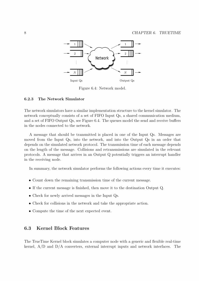
Figure 6.4: Network model.
6.2.3 The Network Simulator
The network simulators have a similar implementation structure to the kernel simulator. Thenetwork conceptually consists of a set of FIFO Input Qs, a shared communication medium,
and a set of FIFO Output Qs, see Figure 6.4. The queues model the send and receive buffersin the nodes connected to the network.
A message that should be transmitted is placed in one of the Input Qs. Messages aremoved from the Input Qs, into the network, and into the Output Qs in an order that
depends on the simulated network protocol. The transmission time of each message dependson the length of the message. Collisions and retransmissions are simulated in the relevant
protocols. A message that arrives in an Output Q potentially triggers an interrupt handlerin the receiving node.
In summary, the network simulator performs the following actions every time it executes:
• Count down the remaining transmission time of the current message.
• If the current message is finished, then move it to the destination Output Q.
• Check for newly arrived messages in the Input Qs.
• Check for collisions in the network and take the appropriate action.
• Compute the time of the next expected event.
6.3 Kernel Block Features
The TrueTime Kernel block simulates a computer node with a generic and flexible real-time
kernel, A/D and D/A converters, external interrupt inputs and network interfaces. The

6.3. KERNEL BLOCK FEATURES 9
block is configured via an initialization script. The script may be parametrized, enabling the
same script to be used for several nodes.
In the initialization script, the programmer may create tasks, timers, interrupt handlers,
semaphores, etc., representing the software executing in the computer node. The initializa-tion script and the code functions may be written in either Matlab code or in C++ code.
In the C++ case, the initialization script, the code functions and the kernel are compiledtogether into a single binary using Matlab’s MEX facility, rendering a much faster simulation.
The TrueTime Kernel block supports various standard preemptive scheduling algorithms
including fixed-priority scheduling and earliest-deadline-first scheduling. It is also possibleto specify a custom scheduling policy by supplying a sorting function for the Ready Q.
The code below shows how a single node can be configured. In the initialization function,fixed-priority scheduling is selected and the network interface is initialized:
function node_init
% Initialize TrueTime kernel
ttInitKernel(0,0,’prioFP’); % nbrOfInputs, nbrOfOutputs, FP scheduling
% Initialize network interface
data.u = 0; % network interrupt handler local variable
ttCreateInterruptHandler(’nw_handler’,1,’ctrlcode’,data);
ttInitNetwork(2,’nw_handler’); % Node #2 in the network
The network interrupt handler is connected to a code function that in this case implementsa simple controller:
function [exectime,data] = ctrlcode(segment,data)
switch segment,
case 1,
msg = ttGetMsg; % retrieve msg from network
y = msg.y; % extract the measurement data
data.u = data.u - y; % compute the control action
exectime = 0.001;
case 2,
newmsg.u = data.u;
ttSendMsg(3, newmsg, 0); % send result to actuator
exectime = -1; % done
end
In the code function above, the simulated execution of the first segment is 1 ms. This

10 CHAPTER 6. TRUETIME
Figure 6.5: Controllers represented using ordinary discrete Simulink blocks may be calledfrom within the code functions. The only requirement is that the blocks are discrete withthe sample time set to one.
means that the delay between reading the incoming message to sending the reply will be atleast 1 ms (more if there is preemption from higher-priority interrupts).
In both the C++ and Matlab-file cases, it is possible to call Simulink block diagrams fromwithin the code functions. This is sometimes a convenient way to implement controllers. The
listing below shows an example where the discrete PI-controller in Figure 6.5 is used in acode function:
function [exectime,data] = PIcode(segment,data)
switch segment,
case 1,
inp(1) = ttAnalogIn(1);
inp(2) = ttAnalogIn(2);
outp = ttCallBlockSystem(2,inp,’PI_Controller’);
data.u = outp(1);
exectime = outp(2);
case 2,
ttAnalogOut(1, data.u);
exectime = -1; % done
end
TrueTime includes a large library of real-time primitives that may be called from theinitialization script and/or the task code. There is support for periodic and aperiodic tasks,
periodic and one-shot timers, hardware or software-triggered interrupts, and task synchro-nization mechanisms in the forms of semaphores, monitors, and mailboxes. It is possible
to on-line read and modify most task attributes (period, deadline, priority, etc.). Advancedreal-time scheduling features include deadline overrun handlers, worst-case execution time
overrun handlers, and the possibility to abort task jobs. Simulation-wise, the user may log
6.4. NETWORK BLOCKS FEATURES 11
various variables relating to the task schedule. Finally, there are primitives for initializing
network interfaces and sending and receiving messages.
6.4 Network Blocks Features
The TrueTime Network block and the TrueTime Wireless Network block simulate the phys-ical layer and the medium-access layer of various local-area networks. The types of networks
supported are CSMA/CD (Ethernet), CSMA/AMP (CAN), Round Robin (Token Bus),FDMA, TDMA (TTP), Switched Ethernet, WLAN (802.11b), and ZigBee (802.15.4). The
blocks only simulate the medium access (the scheduling), possible collisions or interference,and the point-to-point/broadcast transmissions. Higher-layer protocols such as TCP/IP are
not simulated as such but may be implemented as applications in the nodes.
There is also a third network block that simulates the transmission and reception ofultrasound pulses. In this case, no receiver and no data can be specified. This block can be
used to simulate ultrasound-based navigation systems for mobile devices.
The network blocks are mainly configured via their block dialogues. Common parameters
to all types of networks are the bit rate, the minimum frame size, and the network interfacedelay. For each type of network there are a number of further parameters that can be
specified. For instance, for the wireless networks it is possible to specify the transmit power,the receiver signal threshold, the pathloss exponent (or a special pathloss function), the ACK
timeout, the retry limit, and the error coding threshold.
A TrueTime model may contain several network blocks, and each kernel block may be
connected to more than one network. Each network is identified by a number, and each nodeconnected to a network is addressed by a number that is unique to that network.
The network blocks may be used in two different ways. The first way is to have one kernel
block for each node in the network. The tasks inside the kernels can then send and receivearbitrary Matlab structure arrays over the network using certain kernel primitives. This
approach is very flexible but requires some amount of programming to configure the system.The second way is to use the stand-alone network interface blocks. These blocks eliminate
the need of kernel blocks, but they restrict the network packets to contain scalar or vectorsignal values. Finally, it is possible to mix kernel blocks and network interface blocks in the
same network.

12 CHAPTER 6. TRUETIME
6.4.1 Wireless Networks
Compared to the wired network block, the wireless network block has additional x and y
inputs that represent the actual location of the nodes in the network. These inputs can beconnected to further blocks that model the physical movement of the nodes. The current x
and y coordinates of the nodes will influence the signal-to-interference ratio at the receiver.The path-loss of radio signals is modeled as 1/da, where d is the distance between the sending
and the receiving node, and a is an environment parameter (typically in the range from 2to 4). If the received energy is below a user-defined threshold, then no reception will take
place.
A node that wants to transmit a message will proceed as follows. The node first checks
whether the medium is idle. If that has been the case for 50 µs, then the transmission mayproceed. (If not, the node will wait for a random back-off time before the next attempt.) The
signal-to-interference ratio in the receiving node is calculated by treating all simultaneoustransmissions as additive noise. This information is used to determine a probabilistic measure
of the number of bit errors in the received message. If the number of errors is below aconfigurable bit error threshold, then the packet could be successfully received.
6.5 Example: Constant Bandwidth Server
The constant bandwidth server (CBS) [5] is a scheduling server for aperiodic and soft tasksthat executes on top of an EDF scheduler. A CBS is characterized by two parameters: a
server period Ts and a utilization factor Us. The server ensures that the task(s) executingwithin the server can never occupy more than Us of the total CPU bandwidth.
Associated with the server are two dynamic attributes: the server budget cs and theserver deadline ds. Jobs that arrive to the server are placed in a queue and are served on a
first-come, first-served basis. The first job in the queue is always eligible for execution (asan ordinary EDF task), using the current server deadline ds. The server is initialized with
cs := UsTs and ds = Ts. The rules for updating the server are as follows:
1. During the execution of a job, the budget cs is decreased at unit rate.
2. Whenever cs = 0, the budget is recharged to cs := UsTs, and the deadline is postponed
one server period: ds := ds + Ts.
3. If a job arrives at an empty server at time r and cs ≥ (ds − r)Us, then the budget is
recharged to cs := UsTs, and the deadline is set to ds := r + Ts.

6.5. EXAMPLE: CONSTANT BANDWIDTH SERVER 13
The first and second rules limit the bandwidth of the task(s) executing in the server. The
third rule is used to “reset” the server after a sufficiently long idle period.
6.5.1 Implementation of CBS in TrueTime
TrueTime provides a basic mechanism for execution-time monitoring and budgets. The
initial value of the budget is called the WCET (worst-case execution time) of the task. Bydefault, the WCET is equal to the period (for periodic tasks) or the relative deadline (for
aperiodic tasks). The WCET value of a task can be changed by calling ttSetWCET(value,
task). The WCET corresponds to the maximum server budget UsTs in the CBS. The CBS
period is specified by setting the relative deadline of the task. This attribute can be changedby calling ttSetDeadline(value,task).
When a task executes, the budget is decreased at unit rate. The remaining budget can be
checked at any time using the primitive ttGetBudget(task). By default, nothing happenswhen the budget reaches zero. In order to simulate that the task executes inside a CBS, an
execution overrun handler must be attached to the task. A sample initialization script isgiven below:
function node_init
% Initialize kernel, specifying EDF scheduling
ttInitKernel(0,0,’prioEDF’);
% Specify CBS rules for initial deadlines and initial budgets
ttSetKernelParameter(’cbsrules’);
% Specify CBS server period and utilization factor
T_s = 2;
U_s = 0.5;
% Create an aperiodic task
ttCreateTask(’aper_task’,T_s,1,’codeFcn’);
ttSetWCET(T_s*U_s,’aper_task’);
% Attach a WCET overrun handler
ttAttachWCETHandler(’aper_tasl’,’cbs_handler’);
The execution overrun handler can then be implemented as follows:
function [exectime,data] = cbs_handler(seg,data)
% Get the task that caused the overrun
t = ttInvokingTask;
% Recharge the budget

14 CHAPTER 6. TRUETIME
Figure 6.6: TrueTime model of a ball and beam being controlled by a multi-tasking real-timekernel. The Poisson arrivals trigger an aperiodic computation task.
ttSetBudget(ttGetWCET(t),t);
% Postpone the deadline
ttSetAbsDeadline(ttGetAbsDeadline(t)+ttGetDeadline(t),t);
exectime = -1;
If many tasks are to execute inside CBS servers, the same code function can be reused forall the execution overrun handlers.
6.5.2 Experiments
The constant bandwidth server can be used to safely mix hard, periodic tasks with soft,
aperiodic tasks in the same kernel. This is illustrated in the following example, where a balland beam controller should execute in parallel with an aperiodically triggered task. The
Simulink model is shown in Figure 6.6.
The ball and beam process is modelled as a triple integrator disturbed by white noise and
is connected to the TrueTime Kernel block via the A/D and D/A ports. An LQG controllerfor the ball and beam has been designed and is implemented as a periodic task with the
sampling period 10 ms. The computation time of the controller is 5 ms (2 ms for calculatingthe output and 3 ms for updating the controller state). A Poisson source with the intensity
100/s is connected to the Interrupt intput of the kernel, triggering an aperiodic task for eacharrival. The relative deadline of the task is 10 ms, while the execution time of the task is
exponentially distributed with mean 3 ms.
The average CPU utilization of the system is 80%. However, the aperiodic task has a
6.5. EXAMPLE: CONSTANT BANDWIDTH SERVER 15
0 1 2 3 4 5 6 7 8 9 10−0.05
0
0.05
Ou
tpu
t
0 1 2 3 4 5 6 7 8 9 10−50
0
50
Time
Inp
ut
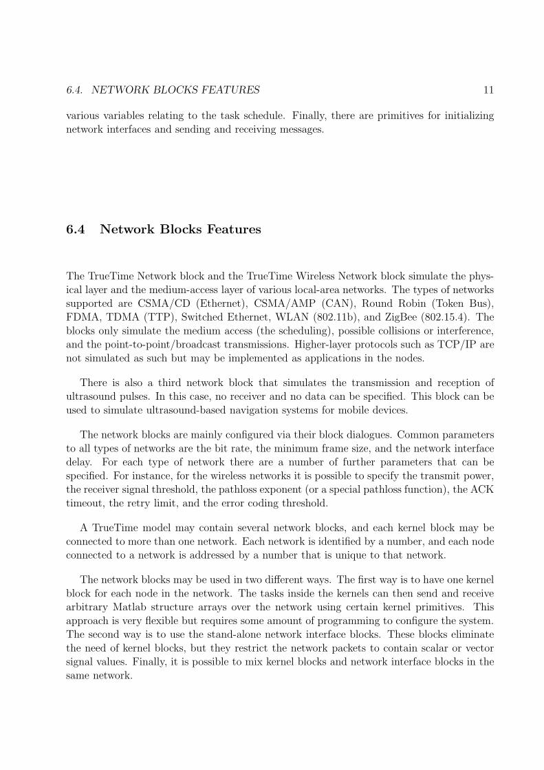
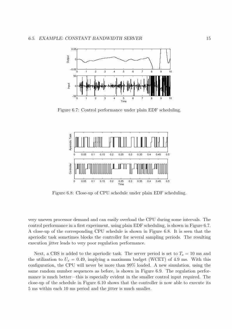
Figure 6.7: Control performance under plain EDF scheduling.
0 0.05 0.1 0.15 0.2 0.25 0.3 0.35 0.4 0.45 0.5
Ap
erio
dic
Ta
sk
0 0.05 0.1 0.15 0.2 0.25 0.3 0.35 0.4 0.45 0.5Time
Co
ntr
olle
r
Figure 6.8: Close-up of CPU schedule under plain EDF scheduling.
very uneven processor demand and can easily overload the CPU during some intervals. The
control performance in a first experiment, using plain EDF scheduling, is shown in Figure 6.7.
A close-up of the corresponding CPU schedule is shown in Figure 6.8. It is seen that theaperiodic task sometimes blocks the controller for several sampling periods. The resulting
execution jitter leads to very poor regulation performance.
Next, a CBS is added to the aperiodic task. The server period is set to Ts = 10 ms andthe utilization to Us = 0.49, implying a maximum budget (WCET) of 4.9 ms. With this
configuration, the CPU will never be more than 99% loaded. A new simulation, using thesame random number sequences as before, is shown in Figure 6.9. The regulation perfor-
mance is much better—this is especially evident in the smaller control input required. Theclose-up of the schedule in Figure 6.10 shows that the controller is now able to execute its
5 ms within each 10 ms period and the jitter is much smaller.

16 CHAPTER 6. TRUETIME
0 1 2 3 4 5 6 7 8 9 10−0.05
0
0.05
Ou
tpu
t
0 1 2 3 4 5 6 7 8 9 10−50
0
50
Time
Inp
ut
Figure 6.9: Control performance under CBS scheduling.
0 0.05 0.1 0.15 0.2 0.25 0.3 0.35 0.4 0.45 0.5
Ap
erio
dic
Ta
sk
0 0.05 0.1 0.15 0.2 0.25 0.3 0.35 0.4 0.45 0.5Time
Co
ntr
olle
r
Figure 6.10: Close-up of CPU schedule under CBS scheduling.
6.6. EXAMPLE: MOBILE ROBOTS IN A SENSOR NETWORK 17
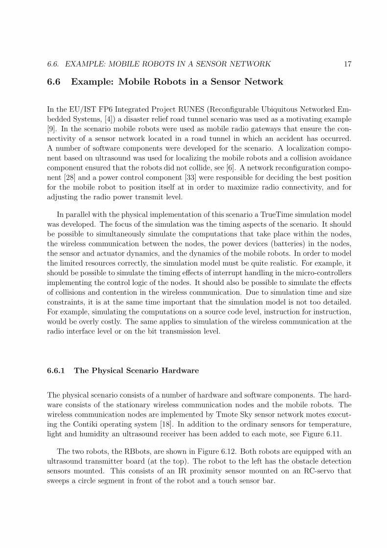
6.6 Example: Mobile Robots in a Sensor Network
In the EU/IST FP6 Integrated Project RUNES (Reconfigurable Ubiquitous Networked Em-
bedded Systems, [4]) a disaster relief road tunnel scenario was used as a motivating example[9]. In the scenario mobile robots were used as mobile radio gateways that ensure the con-
nectivity of a sensor network located in a road tunnel in which an accident has occurred.A number of software components were developed for the scenario. A localization compo-
nent based on ultrasound was used for localizing the mobile robots and a collision avoidancecomponent ensured that the robots did not collide, see [6]. A network reconfiguration compo-
nent [28] and a power control component [33] were responsible for deciding the best positionfor the mobile robot to position itself at in order to maximize radio connectivity, and for
adjusting the radio power transmit level.
In parallel with the physical implementation of this scenario a TrueTime simulation model
was developed. The focus of the simulation was the timing aspects of the scenario. It shouldbe possible to simultaneously simulate the computations that take place within the nodes,
the wireless communication between the nodes, the power devices (batteries) in the nodes,the sensor and actuator dynamics, and the dynamics of the mobile robots. In order to model
the limited resources correctly, the simulation model must be quite realistic. For example, itshould be possible to simulate the timing effects of interrupt handling in the micro-controllers
implementing the control logic of the nodes. It should also be possible to simulate the effectsof collisions and contention in the wireless communication. Due to simulation time and size
constraints, it is at the same time important that the simulation model is not too detailed.For example, simulating the computations on a source code level, instruction for instruction,
would be overly costly. The same applies to simulation of the wireless communication at theradio interface level or on the bit transmission level.
6.6.1 The Physical Scenario Hardware
The physical scenario consists of a number of hardware and software components. The hard-
ware consists of the stationary wireless communication nodes and the mobile robots. Thewireless communication nodes are implemented by Tmote Sky sensor network motes execut-
ing the Contiki operating system [18]. In addition to the ordinary sensors for temperature,light and humidity an ultrasound receiver has been added to each mote, see Figure 6.11.
The two robots, the RBbots, are shown in Figure 6.12. Both robots are equipped with an
ultrasound transmitter board (at the top). The robot to the left has the obstacle detectionsensors mounted. This consists of an IR proximity sensor mounted on an RC-servo that
sweeps a circle segment in front of the robot and a touch sensor bar.

18 CHAPTER 6. TRUETIME
Figure 6.11: Stationary sensor network nodes with ultrasound receiver circuit. The node ispackaged in a plastic box to reduce wear.
Figure 6.12: The two Lund RBbots.
6.6. EXAMPLE: MOBILE ROBOTS IN A SENSOR NETWORK 19
TMote Sky
ATMEL AVR
Mega16
ATMEL AVR
Mega128
Mega16
ATMEL AVR
Mega16
ATMEL AVR
Left Wheel
Motor &
Encoder
Motor &
Encoder
Right Wheel
ObstacleDetectionSensors
Ultrasound
Transmitter
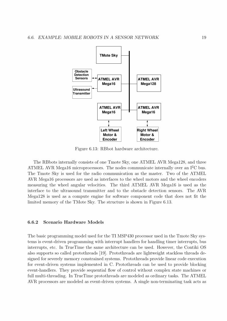
Figure 6.13: RBbot hardware architecture.
The RBbots internally consists of one Tmote Sky, one ATMEL AVR Mega128, and threeATMEL AVR Mega16 microprocessors. The nodes communicate internally over an I2C bus.
The Tmote Sky is used for the radio communication as the master. Two of the ATMEL
AVR Mega16 processors are used as interfaces to the wheel motors and the wheel encodersmeasuring the wheel angular velocities. The third ATMEL AVR Mega16 is used as the
interface to the ultrasound transmitter and to the obstacle detection sensors. The AVRMega128 is used as a compute engine for software component code that does not fit the
limited memory of the TMote Sky. The structure is shown in Figure 6.13.
6.6.2 Scenario Hardware Models
The basic programming model used for the TI MSP430 processor used in the Tmote Sky sys-tems is event-driven programming with interrupt handlers for handling timer interrupts, bus
interrupts, etc. In TrueTime the same architecture can be used. However, the Contiki OSalso supports so called protothreads [19]. Protothreads are lightweight stackless threads de-
signed for severely memory constrained systems. Protothreads provide linear code executionfor event-driven systems implemented in C. Protothreads can be used to provide blocking
event-handlers. They provide sequential flow of control without complex state machines orfull multi-threading. In TrueTime protothreads are modeled as ordinary tasks. The ATMEL
AVR processors are modeled as event-driven systems. A single non-terminating task acts as

20 CHAPTER 6. TRUETIME
the main program and the event-handling is performed in interrupt handlers.
The software executing in the TrueTime processors is written in C++. The names ofthe files containing the code are input parameters of the network blocks. The localization
component consists of two parts. The distance sensor part of the component is implementedas a (proto-)thread in each stationary sensor node. An Extended Kalman Filter-based data
fusion is implemented in the Tmote Sky processor on-board each robot. The localizationmethod makes use of the ultrasound network and the radio network. The collision avoidance
component code is implemented in the ATMEL AVR Mega128 processor using events andinterrupts. It interacts over the I2C bus with the localization component and with the robot
position controller, both located in the Tmote Sky processor.
6.6.3 TrueTime Modeling of Bus Communication
The I2C bus within the RBbots is modeled in TrueTime by a network block. The True-Time network model assumes the presence of a network interface card or a bus controller
implemented either in hardware or software, i.e. as drivers. The Contiki interface to the I2Cbus is software-based and corresponds well to the TrueTime model. In the ATMEL AVRs,
however, it is normally the responsibility of the application programmer to manage all busaccess and synchronization directly in the application code. In the TrueTime model this
low-level bus access is not modeled. Instead it is assumed that there exists a hardware orsoftware bus interface that implements this.
Although the I2C is a multi-master bus that uses arbitration to resolve conflicts this is
not how it is modeled in TrueTime. On the Tmote Sky the radio chip and the I2C bus shareconnection pins. Due to this it is only possible to have one master on the I2C bus and this
master must be the Tmote Sky. All communication must be initiated by the master. Due
to this bus access conflicts are eliminated. Therefore the I2C bus is modeled as a CAN buswith the transmission rate set to match the transmission rate of the I2C bus.
6.6.4 TrueTime Modeling of Radio Communication
The radio communication used by the Tmote Sky is the IEEE 802.15.4 MAC protocol (theso called Zigbee MAC protocol) and the corresponding TrueTime wireless network protocol
was used. The requirements on the simulation environment from the network reconfigurationand radio power control components are that it should be possible to change the transmit
power of the nodes and that it should be possible to measure the received signal strength,i.e., the so called Received Signal Strength Indicator (RSSI). The former is possible through
the TrueTime command ttSetNetworkParameter(’transmitpower’,value). The RSSI is
6.6. EXAMPLE: MOBILE ROBOTS IN A SENSOR NETWORK 21
obtained as an optional return value of the TrueTime function ttGetMsg.
In order to model the ultrasound a special block was developed. The block is a specialversion of the wireless network block that models the ultrasound propagation of a transmitted
ultrasound pulse. The main difference between the wireless network block and the ultrasoundblock is that in the ultrasound block it is the propagation delay that is important, whereas in
the ordinary wireless block it is the medium access delay and the transmission delay that aremodeled. The ultrasound is modeled as a single sound pulse. When it arrives at a stationary
sensor node an interrupt is generated. This also differs from the physical scenario, in whichthe ultrasound signal is connected via an AD converter to the Tmote Sky.
The network routing is implemented using a TrueTime model of the AODV routing
protocol, [29], commonly used in sensor network and mobile robot applications. AODV uses
three basic types of control messages in order to build and invalidate routes: route request(RREQ), route reply (RREP), and route error (RERR) messages. These control messages
contain source and destination sequence numbers, which are used to ensure fresh and loop-free routes. A node that requires a route to a destination node initiates route discovery
by broadcasting an RREQ message to its neighbors. A node receiving an RREQ starts byupdating its routing information backwards towards the source. If the same RREQ has not
been received before, the node then checks its routing table for a route to the destination. If aroute exists with a sequence number greater than or equal to that contained in the RREQ, an
RREP message is sent back towards the source. Otherwise, the node rebroadcasts the RREQ.When an RREP has propagated back to the original source node, the established route
may be used to send data. Periodic hello messages are used to maintain local connectivityinformation between neighboring nodes. A node that detects a link break will check its
routing table to find all routes which use the broken link as the next hop. In order topropagate the information about the broken link, an RERR message is then sent to each
node that constitute a previous hop on any of these routes.
Two TrueTime tasks are created in each node to handle AODV send and receive actions,
respectively. The AODV send task is activated from the application code as a data messageshould be sent to another node in the network. The AODV receive task handles incoming
AODV control messages and forwarding of data messages. Communication between theapplication layer and the AODV layer is handled using TrueTime mailboxes. Each node also
contains a periodic task, responsible for broadcasting hello messages and determine localconnectivity based on hello messages received from neighboring nodes. Finally, each node
has a task to handle timer expiry of route entries.
The AODV protocol in TrueTime is implemented in such a way that it stores messages
to destinations for which no valid route exists, at the source node. This means that when,eventually, the network connectivity has been restored through the use of the mobile radio
gateways, the communication traffic will be automatically restored.

22 CHAPTER 6. TRUETIME
Figure 6.14: The TrueTime model diagram. In order to reduce the use of wires From and Toblocks hidden inside the corresponding subsystems are used to connect the stationary sensornodes to the radio and ultrasound networks.
6.6.5 The Complete Model
In addition to the above the complete model for the scenario also contains models of the
sensors, motors, robot dynamics, and a world model that keeps track of the position of therobots and the fixed obstacles within the tunnel.
The wheel motors are modeled as first-order linear systems plus integrators with the
angular velocities and positions as the outputs. From the motor velocities the corresponding
wheel velocities are calculated. The wheel positions are controlled by two PI-controllersresiding in the ATMEL AVR processors acting as interfaces to the wheel motors.
The Lund RBbot is a dual-drive unicycle robot. It is modeled as a third-order system
px =1
2(R1ω1 + R2ω2) cos(θ)
py =1
2(R1ω1 + R2ω2) sin(θ)
θ =1
D(R2ω2 − R1ω1)
(6.1)
where the state consists of the x- and y-positions and the heading θ. Input to the system
are the angular velocities ω1 and ω2 of the two wheels. The parameters R1 and R2 are theradius of the two wheels and D is the distance between the wheels.
The top-level TrueTime model diagram is shown in Fig. 6.14. The stationary sensor
nodes are implemented as Simulink subsystems that internally contain a TrueTime kernel

6.6. EXAMPLE: MOBILE ROBOTS IN A SENSOR NETWORK 23
modeling the Tmote Sky mote and connections to the radio network and the ultrasound
communication blocks. In order to reduce the wiring From and To blocks hidden inside thecorresponding subsystems are used for the connections. The block handling the dynamic
animation is not shown in the figure.
The subsystem for the mobile robots is shown in Fig. 6.15. The Robot Dynamics block
contains the motor models and the robot dynamics model.
The position of the robots and status of the stationary sensor nodes, i.e., whether theyare operational or not, are shown in a separate animation workspace, see Fig. 6.16.
6.6.6 Evaluation
The implemented TrueTime model contains several simplifications. For example, interruptlatencies are not simulated, only context switch overheads. All execution times are chosen
based on experience from the hardware implementation. Also, it is important to stress thatthe simulated code is only a model of the actual code that executes in the sensor nodes
and in the robots. However, since C is the programming language used in both cases thetranslation is in most cases quite straightforward.
In spite of the above it is our experience that the TrueTime simulation approach givesresults that are close to the real case. The TrueTime approach has also been validated by
others. In [11] a TrueTime-based model is compared with a hardware-in-the-loop (HIL)model of a distributed CAN-based control system. The TrueTime simulation result matched
the HIL results very well.
An aspect of the model that is extremely difficult, if not impossible, to validate is thewireless communication. Simulation of wireless MANET systems is notoriously difficult, see,
e.g., [7]. The effects of multi-path propagation, fading, and external disturbances are very
difficult to model accurately. The approach adopted here is to first start with an idealizedexponential decay ratio model and then, when this works properly, gradually add more and
more non-determinism. This can be done either by setting a high probability that a packetis lost, or by providing a user-defined radio model using Rayleigh fading.
The total code size for the model was 3,7k lines of C code. Parts of the algorithmic
code, e.g., the Extended Kalman filter code, were exactly the same as in the real robots.The model contained five kernel blocks and one network block per robot, one kernel block
per sensor node, with six sensors, one wireless network block for the radio traffic, and oneultrasound block modeling the ultrasound propagation. The simulation rate was slightly
faster than real time, executing on an ordinary dual-core Windows laptop.

24 CHAPTER 6. TRUETIME
Tmote Sky
AVR Mega16−1
AVR Mega128
AVR Mega16−2
AVR Mega16−3
Robot Dynamics
I2C Bus
To RadioNetwork
From RadioNetwork
To UltrasoundNetwork
2
y
1
x
[radio2]A/D
Interrupts
Rcv
D/A
Snd
Schedule
Monitors
P
left
right
x
y
theta
lspeed
rspeed
In1
In2
In3
In4
In5
Out1
Out2
Out3
Out4
Out5
[ultra1]
[radio1]
A/D
Interrupts
Rcv
D/A
Snd
Schedule
Monitors
P
A/D
Interrupts
Rcv
D/A
Snd
Schedule
Monitors
P
A/D
Interrupts
Rcv
D/A
Snd
Schedule
Monitors
P
A/D
Interrupts
Rcv
D/A
Snd
Schedule
Monitors
P
Figure 6.15: The Simulink model of the mobile robots. For the sake of clarity the obstacledetection sensors have been omitted. These should be connected to AVR Mega16-1.

6.7. EXAMPLE: NETWORK INTERFACE BLOCKS 25
Figure 6.16: Animation workspace
6.7 Example: Network Interface Blocks
The last example illustrates how the new, stand-alone network interface blocks can be usedto simulate time-triggered or event-triggered networked control loops. In this case, because
there are no kernel blocks, no initialization scripts or code functions must be written.
The networked control system in this example consists a plant (an integrator), a network,
and two nodes: an IO device (handling AD and DA conversion) and a controller node. At theIO node, the process is sampled by a ttSendMsg network interface block, which transmits the
value to the controller node. There, the packet is received by a ttGetMsg network interfaceblock. The control signal is computed and the control is transmitted back to the IO node
by another ttSendMsg block. Finally, the signal is received by a ttGetMsg block at the IOand actuated to the process.
Two versions of the control loop will be studied. In Fig. 6.17, both ttSendMsg blocksare time-triggered. The process output is sampled every 0.1 s, and a new control signal is
computed with the same interval but with a phase shift of 0.05 s. The resulting controlperformance and network schedule is shown in Fig. 6.18. The process output is kept close
to zero despite the process noise. The schedule shows that the network load is quite high.
In the second version of the control loop, the ttSendMsg blocks are event-triggered instead,see Fig. 6.19. A sample is generated whenever the magnitude of the process output passes
0.25. The arrival of a measurement sample at the controller node triggers—after a delay—the computation and sending of the control signal back to the IO node. The resulting control
performance and network schedule is shown in Fig. 6.20. It can be seen that the process is

26 CHAPTER 6. TRUETIME
Figure 6.17: Time-triggered networked control system using the stand-alone network inter-face blocks. The ttSendMsg blocks are driven by periodic pulse generators.
0 2 4 6 8 10−1
0
1
Pro
cess O
utp
ut
0 2 4 6 8 10Time
Netw
ork
Schedule
Figure 6.18: Plant output and network schedule for the time-triggered control system.

6.8. LIMITATIONS AND EXTENSIONS 27
Figure 6.19: Event-triggered networked control system using the stand-alone network inter-face blocks. The process output is sampled by the ttSendMsg block when the magnitudeexceeds a certain threshold.
still stabilized, although much fewer network messages are sent.
6.8 Limitations and Extensions
Although TrueTime is quite powerful it has some limitations. Some of them could be removed
by extending TrueTime in different directions. This will be discussed here.
0 2 4 6 8 10−1
0
1
Pro
cess O
utp
ut
0 2 4 6 8 10Time
Netw
ork
Schedule
Figure 6.20: Plant output and network schedule for the event-triggered control system.
28 CHAPTER 6. TRUETIME
6.8.1 Single Core Assumption
Multi-core architectures are currently being increasingly common also in embedded systems.
The TrueTime kernel, however, is single core. Modifying the kernel to instead support aglobally scheduled, i.e., a single ready queue, shared memory multi-core platform is probably
relatively straightforward. However, to support a partitioned system with separate readyqueues, separate caches, and task migration overheads, etc., is most likely outside the scope.
6.8.2 Execution Times
In TrueTime it is the user responsibility to assign the execution times of the different codesegments. This should correspond to the amount of time it should take to execute the code on
the particular target machine where it should run. For small micro-controllers it is possible toperform these assessments fairly well. However, for normal size platforms it is difficult to get
good estimates. The problem can be compared with the problem of performing worst-caseexecution time analysis.
The idea behind the TrueTime approach is that the execution times should be viewed
as design parameters. By increasing or decreasing them a different processor speeds can besimulated. By adding a random element to them variations in execution times due to code
branches and data-dependent execution time statements can be accounted for. However, in
a real system the execution time of a piece of code can be divided in two parts. The firstpart is the execution of the different instructions in the code. This is fairly straightforward
to estimate. The second part is the time caused by the hardware platform. This includesthe time caused by cache misses, pipeline breaks, memory access latencies, etc. This time
is more difficult to get good estimates for. A possible approach is to have this part of theexecution time added to the user-provided times automatically by the kernel block based on
different parametrized assumptions on the hardware platform.
6.8.3 Single Thread Execution
Since Simulink simulation is performed by a single execution thread the multi-tasking in
the kernel block has to be emulated. One consequence of this is that it is the responsibilityof the user that the context of each task is saved and restored in the correct way. This
is done by passing the context as argument to the code functions. Another partly relatedconsequence of this is the segmentation that has do be applied to every task. The latter is
the main reason why it is not possible to use production C code in TrueTime simulations.In addition, a code function may not call other code functions, i.e., abstractions on the code
function level are not supported.

6.9. SUMMARY 29
Preliminary investigations indicates that it should be possible to map the TrueTime tasks
onto Posix threads, i.e., to use multiple threads inside each kernel S-function. Using thisapproach it would the problem with the task context and segments would be solved auto-
matically.
6.8.4 Simulation Platform
TrueTime is based on Simulink. This is both an advantage and a disadvantage. It is
good since it makes it easy for existing Matlab/Simulink users to start using it. However,Matlab/Simulink is still not widely spread in the computer science community. The threshold
for a non-Simulink user to start using TrueTime is therefore fairly high. An advantage with
building upon Matlab is the vast availability of other toolboxes that can be combined withTrueTime.
However, it is possible to port TrueTime to other platforms. In [22] a feasibility study is
presented where the kernel block of TrueTime is ported to Scilab/Scicos. Also, in the newEuropean ITEA 2 project EUROSYSLIB the TrueTime network block are being ported to
the Modelica/Dymola platform.
6.8.5 Higher Layer Protocols
The network blocks only support link layer protocols. In most cases this is enough, since
most real-time networks are local area networks without any routing or transport layers.However, if higher layer protocols are needed, these are not directly supported by TrueTime.
The examples contain a TCP transport protocol example and an AODV routing protocolexample, but these applications are implemented as application code. It would be interesting
to provide built-in support also for some of the most popular higher-order protocols. It wouldalso be useful to have a plug-and-play facility that would make it easy for the user to add
new protocols to the networks blocks. Currently this involves modifications of the C++network block source code.
6.9 Summary
This chapter has presented TrueTime, a freeware extension to Simulink that allows multi-
threaded real-time kernels and communication networks to be simulated in parallel with theplant dynamics. Having been developed over almost ten years, TrueTime has several more
features than those mentioned in this chapter. For a complete description, please see the

30 CHAPTER 6. TRUETIME
latest version of the reference manual (e.g., [25]). In particular, many features related to
real-time scheduling have been omitted.
References
[1] NAB (Network in A Box). Home page: http://nab.epfl.ch/, 2004.[2] ns-2. Home page: http://www.isi.edu/nsnam/ns/, 2008.
[3] Omnet++. Home page: http://www.omnetpp.org, 2008.[4] RUNES – Reconfigurable Ubiquitous Networked Embedded Systems. Home page:
http://www.ist-runes.org/, 2008.[5] Luca Abeni and Giorgio Buttazzo. Integrating multimedia applications in hard real-time
systems. In Proc. 19th IEEE Real-Time Systems Symposium, Madrid, Spain, 1998.
[6] P. Alriksson, J. Nordh, K.-E. Arzen, A. Bicchi, A. Danesi, R. Schiavi, and L. Pallottino.A component-based approach to localization and collision avoidance for mobile multi-
agent systems. In Proceedings of the European Control Conference (ECC), Kos, Greece,Kos, Greece, 2007.
[7] T.R. Andel and A. Yasinac. On the credibility of manet simulations. IEEE Computer,pages 48–54, July 2006.
[8] Martin Andersson, Dan Henriksson, Anton Cervin, and Karl-Erik Arzen. Simulationof wireless networked control systems. In Proceedings of the 44th IEEE Conference
on Decision and Control and European Control Conference ECC 2005, Seville, Spain,December 2005.
[9] K.-E. Arzen, A. Bicchi, G. Dini, S. Hailes, K.H. Johansson, J. Lygeros, and A. Tzes. Acomponent-based approach to the design of networked control systems. In Proceedings
of the European Control Conference (ECC), Kos, Greece, Kos, Greece, 2007.[10] N. Audsley, A. Burns, M. Richardson, and A. Wellings. STRESS—A simulator for hard
real-time systems. Software—Practice and Experience, 24(6):543–564, June 1994.
[11] D. Ayavoo, M.J. Pont, and S. Parker. Using simulation to support the design of dis-tributed embedded control systems: a case study. In In Proceedings of 1st UK Embedded
Forum, Brimingham, UK, 2004.[12] Philip Baldwin, Sanjeev Kohli, Edward A. Lee, Xiaojun Liu, and Yang Zhao. Mod-
eling of sensor nets in Ptolemy II. In IPSN’04: Proceedings of the third internationalsymposium on Information processing in sensor networks, pages 359–368. ACM Press,
2004.[13] Michael Branicky, Vincenzo Liberatore, and Stephen M. Phillips. Networked control
systems co-simulation for co-design. In Proc. American Control Conference, 2003.[14] A. Casile, G. Buttazzo, G. Lamastra, and G. Lipari. Simulation and tracing of hybrid
task sets on distributed systems. In Proc. 5th International Conference on Real-TimeComputing Systems and Applications, 1998.
[15] Anton Cervin, Dan Henriksson, Bo Lincoln, Johan Eker, and Karl-Erik Arzen. How

6.9. SUMMARY 31
does control timing affect performance? IEEE Control Systems Magazine, 23(3):16–30,
June 2003.[16] Michael I. Clune, Pieter J. Mosterman, and Christos G. Cassandras. Discrete event
and hybrid system simulation with simEvents. In Proceedings of the 8th International
Workshop on Discrete Event Systems, Ann Arbor, Michigan, USA, 2006.[17] J.-M. Dricot and P. De Doncker. High-accuracy physical layer model for wireless net-
work simulations in NS-2. In In Proceedings of the Int. Workshop on Wireless Ad-HocNetworks (IWWAN), Oulu, Finland, 2004.
[18] Adam Dunkels, Bjorn Gronvall, and Thiemo Voigt. Contiki - a lightweight and flexibleoperating system for tiny networked sensors. In Proceedings of the First IEEE Workshop
on Embedded Networked Sensors (Emnets-I), Tampa, Florida, USA, November 2004.[19] Adam Dunkels, Oliver Schmidt, Thiemo Voigt, and Muneeb Ali. Protothreads: Simpli-
fying event-driven programming of memory-constrained embedded systems. In Proceed-ings of the Fourth ACM Conference on Embedded Networked Sensor Systems (SenSys
2006), Boulder, Colorado, USA, November 2006.[20] Johan Eker and Anton Cervin. A Matlab toolbox for real-time and control systems
co-design. In Proceedings of the 6th International Conference on Real-Time ComputingSystems and Applications, Hong Kong, P.R. China, December 1999. Best student paper
award.
[21] Jad El-Khoury and M. Torngren. Towards a toolset for architectural design of dis-tributed real-time control systems. In Proceedings of the 22nd IEEE Real-Time Systems
Symposium, London, England, December 2001.[22] Daniel Kusnadi. TrueTime in Scicos. Master’s Thesis ISRN LUTFD2/TFRT--5799-
-SE, Department of Automatic Control, Lund University, Sweden, June 2007.[23] Philip Levis, Nelson Lee, Matt Welsh, and David Culler. TOSSIM: accurate and scal-
able simulation of entire TinyOS applications. In Proceedings of the 1st internationalconference on Embedded networked sensor systems, pages 126–137, Los Angeles, CA,
USA, 2003.[24] P.S. Magnusson. Simulation of parallel hardware. In In Proceedings of the Int. Workshop
on Modeling Analysis and Simulation of Computer And Telecommunication Systems(MASCOTS), San Diego, CA, 1993.
[25] Martin Ohlin, Dan Henriksson, and Anton Cervin. TrueTime 1.5—Reference Manual,January 2007. Available at http://www.control.lth.se/truetime.
[26] Fredrik Osterlind. A Sensor Network Simulator for the Contiki OS. Technical Report
T2006-05, SICS – Swedish Institute of Computer Science, February 2006.[27] L. Palopoli, L. Abeni, and G. Buttazzo. Real-time control system analysis: An in-
tegrated approach. In Proceedings of the 21st IEEE Real-Time Systems Symposium,Orlando, Florida, December 2000.
[28] A. Panousopoulou and A. Tzes. Utilization of mobile agents for Voronoi-based hetero-geneous wireless sensor network reconfiguration. In Proceedings of the European Control
Conference (ECC), Kos, Greece, Kos, Greece, 2007.

32 CHAPTER 6. TRUETIME
[29] C.E. Perkins and E.M. Royer. Ad-hoc on-demand distance vector (AODV) routing. In
Proceedings of the 2nd IEEE Workshop on Mobile Computing Systems and Applications,New Orleans, LA, 1999.
[30] F. Singhoff, J. Legrand, L. Nana, and L. Marce. Cheddar: a flexible real time scheduling
framework. ACM SIGAda Ada Letters, 24(4):1–8, 2004.[31] M. F. Storch and J. W.-S. Liu. DRTSS: A simulation framework for complex real-time
systems. In Proc. 2nd IEEE Real-Time Technology and Applications Symposium, 1996.[32] H.-Y. Tyan. Design, realization and evaluation of a component-based compositional
software architecture for network simulation. PhD thesis, Ohio State University, 2002.[33] B. Zurita Ares, C. Fischione, A. Speranzon, and K.H. Johansson. On power control
for wireless sensor networks: radio model, software implementation and experimentalevaluation. In Proceedings of the European Control Conference (ECC), Kos, Greece,
Kos, Greece, 2007.