tuanv.nguyen%% - garvan.org.au · analysis using r # read data into r wt = read.csv("~/google...

Tuan V. Nguyen Garvan Ins)tute of Medical Research

Sydney, Australia

Garvan Ins)tute Biosta)s)cs Seminar 18/8/2015 © Tuan V. Nguyen

Analysis of covariance (ANCOVA)

•  Example of Before-‐AMer study

•  Problems with percentage change

•  Introduc)on to ANCOVA

Case 1: Goat study

•  40 goats were randomized into two groups of treatment (intensive and standard, 20 each)

•  Outcome: weight gain

•  Aim: to test for the efficacy of treatment

How to assess treatment effect

Common strategy

•  Calculage percentage weight gain = (post-‐treatment – baseline)/baseline * 100

•  Test for difference in weight gain between treatment groups (using t-‐test)

How to assess the efficacy?

Strategy 2

•  Use t-‐test to compare post-‐treatment weight between treatment groups

•  (Assuming that baseline weight is comparable between treatment groups)

Analysis using R

# Read data into R

wt = read.csv("~/Google Drive/Garvan Lectures 2014/ANCOVA/goats.csv", header=T)

# Calculate percentage change

wt$PCT = ((wt$PostWt / wt$BaselineWt)-1)*100

attach(wt)

# analysis

boxplot(PCT ~ Treatment, col="blue")

hist(PCT, breaks=10, col="blue", border="white")

t.test(PCT ~ Treatment)

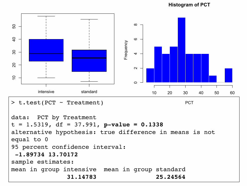
intensive standard

1020

3040

50

> t.test(PCT ~ Treatment)

data: PCT by Treatmentt = 1.5319, df = 37.991, p-value = 0.1338alternative hypothesis: true difference in means is not equal to 095 percent confidence interval: -1.89734 13.70172sample estimates:mean in group intensive mean in group standard 31.14783 25.24564

Histogram of PCT

PCT

Frequency

10 20 30 40 50 60

02

46

8

Problems with the analysis

•  Percentage change (PCT) is a bad choice of effect metric

•  Theore9cal: PCT maps two-‐dimensional data into one-‐vector data

•  Bias: es)mated PCT is NOT equal to the true PCT

•  Sta9s9cal inefficiency: PCT is a ra)o, very sensi)ve to baseline data

•  OMen non-‐normally distributed

Regression toward the mean (RCT)

•  Offspring of tall parents tended to be shorter than their parents

•  Offsprings of short parents tended to be taller than their parents

Sir Francis Galton (1822 -‐ 1911)

This can be proved by mathema9cs (easily!)

A real example from the goat study

10

20

30

40

50

60

17.5 20.0 22.5 25.0 27.5 30.0BaselineWt

PCT

library(ggplot2)qplot(BaselineWt, PCT, color=Treatment, data=wt, geom=c("point", "smooth"), method="lm")

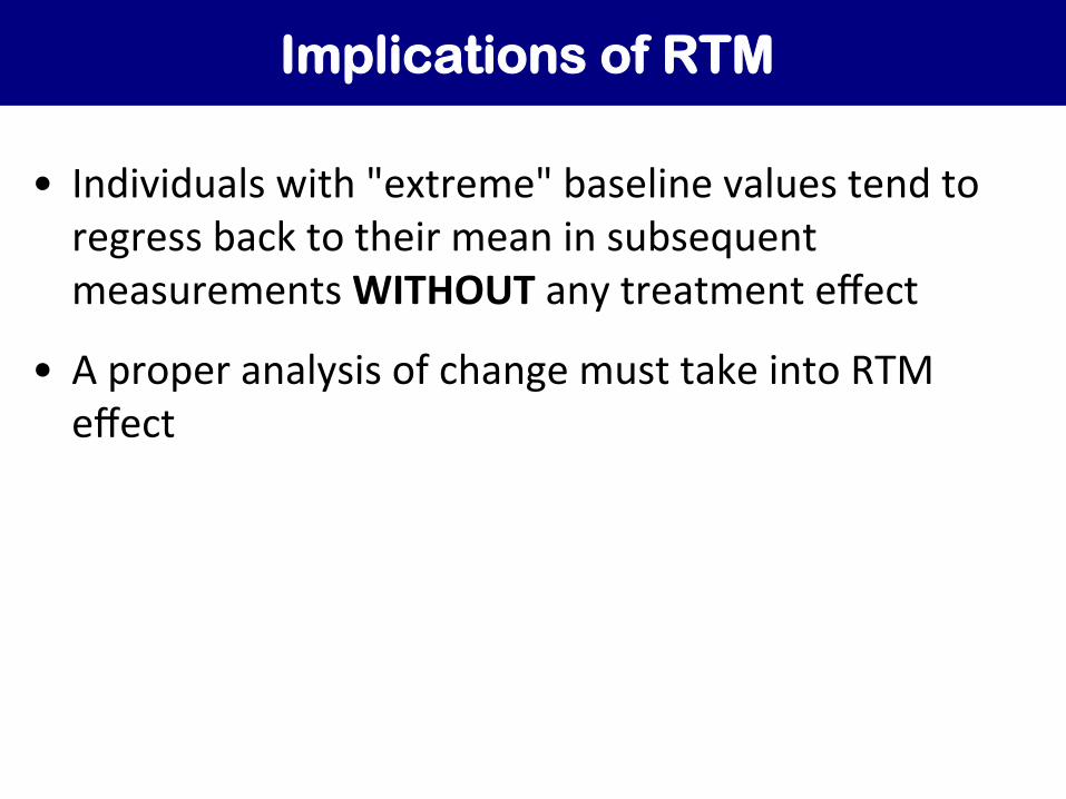
Implications of RTM

•  Individuals with "extreme" baseline values tend to regress back to their mean in subsequent measurements WITHOUT any treatment effect

•  A proper analysis of change must take into RTM effect

Analysis of Covariance Analysis of Covariance

Solution: Analysis of Covariance (ANCOVA)

•  A form of mul)ple linear regression analysis

•  Informal statement:

Y = intercept + effect of covariate + effect of treatment + random error

• Where "covariate" is a confounding factor (eg baseline scores, other factors)

ANCOVA for the goat study

•  Let Y = post-‐treatment scores; X = pre-‐treatment scores; T = treatment effect; and e = random error

•  A formal model for an individual i is:

Yi = α + βXi + γTi + εi

•  Thus, if T = 0, the mean value

Ŷ = α + β*mean(X)

and if T = 1,

Ŷ = α + β*mean(X) + γ = α + β*mean(X) + γ

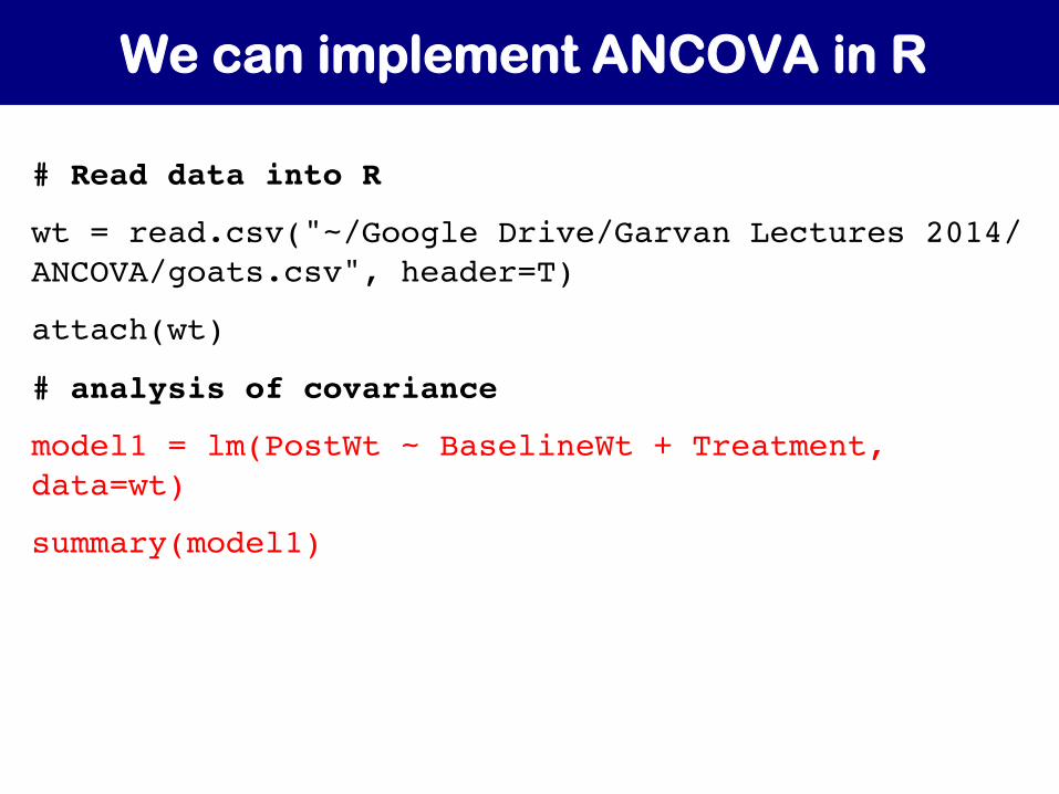
We can implement ANCOVA in R

# Read data into R

wt = read.csv("~/Google Drive/Garvan Lectures 2014/ANCOVA/goats.csv", header=T)

attach(wt)

# analysis of covariance

model1 = lm(PostWt ~ BaselineWt + Treatment, data=wt)

summary(model1)

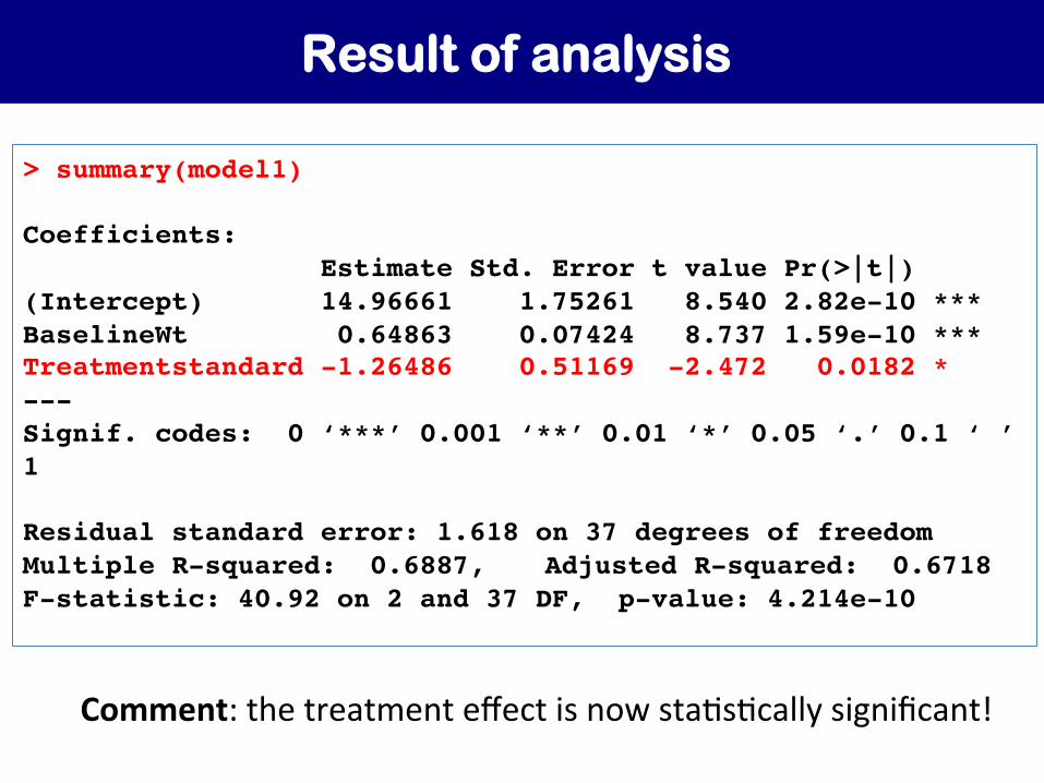
Result of analysis

> summary(model1)

Coefficients: Estimate Std. Error t value Pr(>|t|) (Intercept) 14.96661 1.75261 8.540 2.82e-10 ***BaselineWt 0.64863 0.07424 8.737 1.59e-10 ***Treatmentstandard -1.26486 0.51169 -2.472 0.0182 * ---Signif. codes: 0 ‘***’ 0.001 ‘**’ 0.01 ‘*’ 0.05 ‘.’ 0.1 ‘ ’ 1

Residual standard error: 1.618 on 37 degrees of freedomMultiple R-squared: 0.6887, Adjusted R-squared: 0.6718 F-statistic: 40.92 on 2 and 37 DF, p-value: 4.214e-10

Comment: the treatment effect is now sta)s)cally significant!

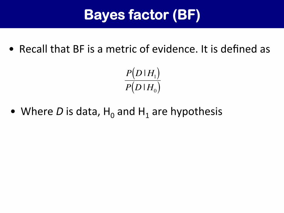
Bayes factor (BF)

•  Recall that BF is a metric of evidence. It is defined as

€

P D |H1( )P D |H0( )

• Where D is data, H0 and H1 are hypothesis

Interpretation of BF

BF Interpreta9on

>100 Decisively favors H1

30 to 100 Very strong evidence for H1

10 to 30 Strong evidence for H1

3 to 10 Substan)al evidence for H1

1 to 3 Weak evidence for H1

1 No evidence

0.3 to 1 Weak evidence for H0

0.1 to 0.3 Substan)al evidence for H0

0.03 to 0.1 Strong evidence for H0

0.01 to 0.03 Very strong evidence for H0

<0.01 Decisive evidence for H0

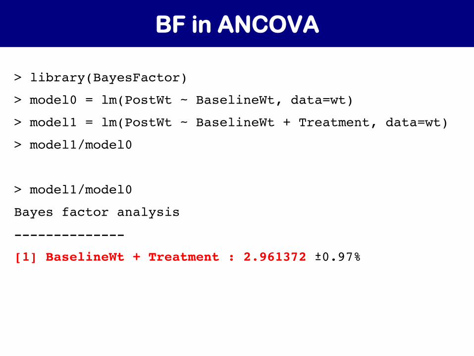
BF in ANCOVA

> library(BayesFactor)

> model0 = lm(PostWt ~ BaselineWt, data=wt)

> model1 = lm(PostWt ~ BaselineWt + Treatment, data=wt)

> model1/model0

> model1/model0

Bayes factor analysis

--------------

[1] BaselineWt + Treatment : 2.961372 ±0.97%

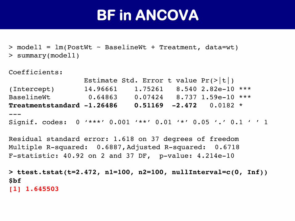
BF in ANCOVA

> model1 = lm(PostWt ~ BaselineWt + Treatment, data=wt)> summary(model1)

Coefficients: Estimate Std. Error t value Pr(>|t|) (Intercept) 14.96661 1.75261 8.540 2.82e-10 ***BaselineWt 0.64863 0.07424 8.737 1.59e-10 ***Treatmentstandard -1.26486 0.51169 -2.472 0.0182 * ---Signif. codes: 0 ‘***’ 0.001 ‘**’ 0.01 ‘*’ 0.05 ‘.’ 0.1 ‘ ’ 1

Residual standard error: 1.618 on 37 degrees of freedomMultiple R-squared: 0.6887,Adjusted R-squared: 0.6718 F-statistic: 40.92 on 2 and 37 DF, p-value: 4.214e-10

> ttest.tstat(t=2.472, n1=100, n2=100, nullInterval=c(0, Inf))$bf[1] 1.645503

Interac9on effect Analysis of Covariance

No interaction effect

INCOME

100000 80000 60000 40000 20000 0

HA

PP

Y

10

9

8

7

6

5

4

3

2

1 0

Men

Women

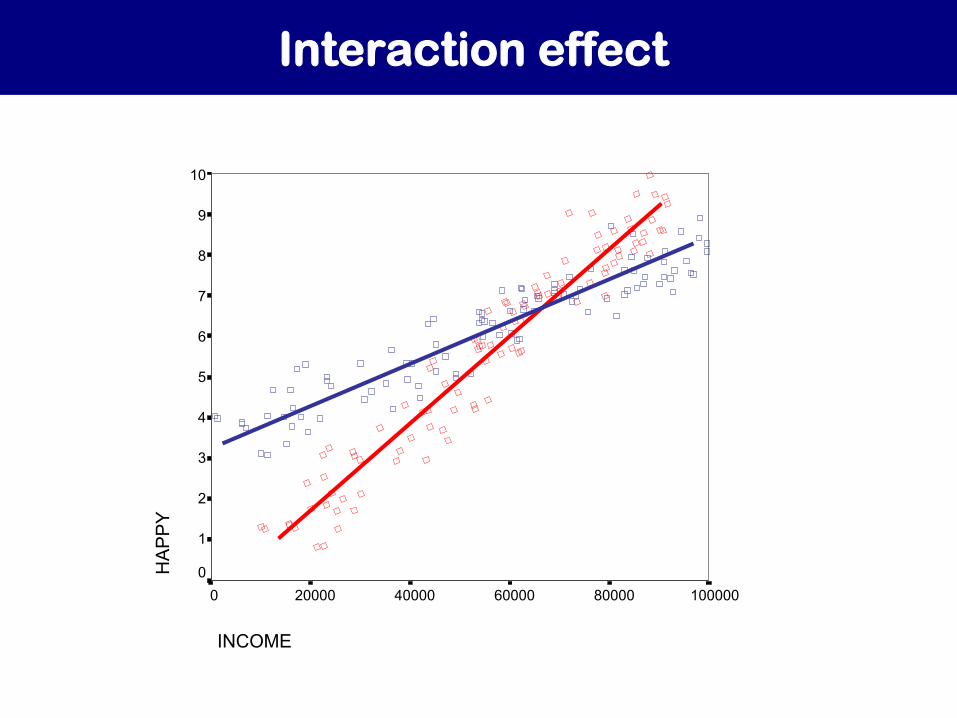
Interaction effect

INCOME

100000 80000 60000 40000 20000 0

HA

PP

Y

10

9

8

7

6

5

4

3

2

1 0

Concept of "interaction"

•  “Differences in the rela)onship (slope) between two variables for each category of a third variable”

•  The rela9onship between X and Y is dependent on a third variable Z

Men: Happy = a1 + b1*income + e

Women: Happy = a2 + b2*income + f

Interac9on is present when b1 ≠ b2

RCT of depression

•  Aim: to es)mate the efficacy of an an)depressant (imipramine) and cogni)ve behavior rx (CBT)

•  Design: Randomized controlled trial, pa)ents were randomized into 4 groups:

– Double placebo (placebo drug and placebo CBT, n=35) –  Imipramine and placebo CBT (n = 35)

–  Placebo imipramine and CBT (n = 35)

–  Imipramine and CBT (n = 35)

Results


Strategy 1

•  Calculate difference between baseline and post-‐treatment (Diff)

•  Use t-‐test to compare Diff between Cogni)ve Rx and placebo


Strategy 2

•  Use analysis of covariance (ANCOVA) to compare post-‐treatment scores between Imipramine and placebo, adjus9ng for baseline scores

R codes for the RCT

dep = read.csv("~/Google Drive/Garvan Lectures 2014/ANCOVA/ancova.csv", header=T)

head(dep)

attach(dep)

plot(PostScore ~ BaselineScore, pch=16, col="blue")

15 20 25 30 35

1015

2025

30

BaselineScore

PostScore

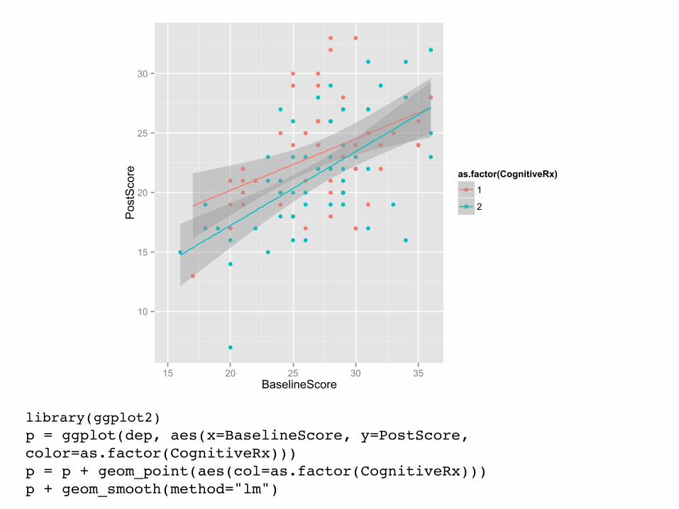
library(ggplot2)p = ggplot(dep, aes(x=BaselineScore, y=PostScore, color=as.factor(CognitiveRx)))p = p + geom_point(aes(col=as.factor(CognitiveRx)))p + geom_smooth(method="lm")

10

15

20

25

30

15 20 25 30 35BaselineScore

PostScore as.factor(CognitiveRx)

1

2

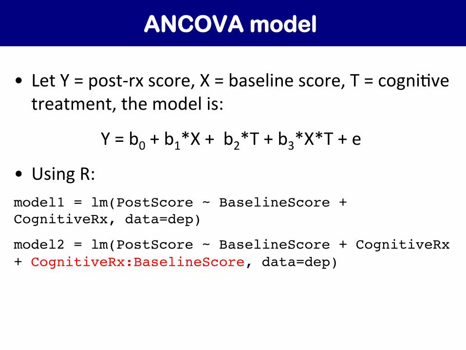
ANCOVA model

•  Let Y = post-‐rx score, X = baseline score, T = cogni)ve treatment, the model is:

Y = b0 + b1*X + b2*T + b3*X*T + e

•  Using R: model1 = lm(PostScore ~ BaselineScore + CognitiveRx, data=dep)

model2 = lm(PostScore ~ BaselineScore + CognitiveRx + CognitiveRx:BaselineScore, data=dep)

> summary(model1)

Coefficients: Estimate Std. Error t value Pr(>|t|) (Intercept) 10.38177 2.51911 4.121 7.46e-05 ***BaselineScore 0.53552 0.08181 6.546 2.11e-09 ***CognitiveRx -1.62178 0.75895 -2.137 0.0349 * ---Signif. codes: 0 ‘***’ 0.001 ‘**’ 0.01 ‘*’ 0.05 ‘.’ 0.1 ‘ ’ 1

Residual standard error: 3.974 on 107 degrees of freedom (30 observations deleted due to missingness)Multiple R-squared: 0.3055, Adjusted R-squared: 0.2925 F-statistic: 23.54 on 2 and 107 DF, p-value: 3.379e-09

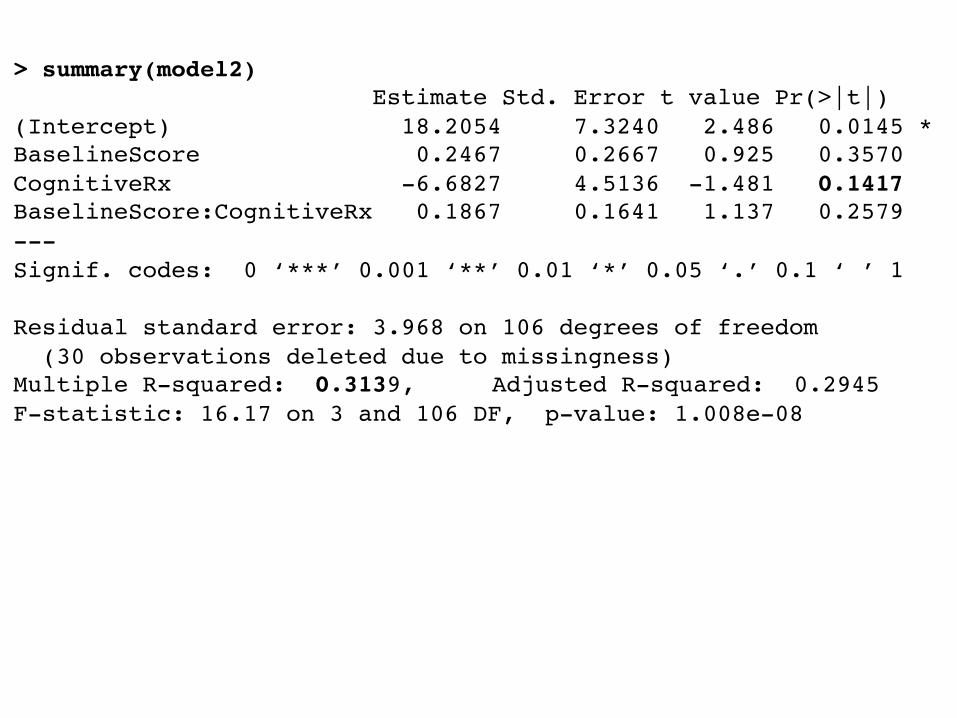
> summary(model2) Estimate Std. Error t value Pr(>|t|) (Intercept) 18.2054 7.3240 2.486 0.0145 *BaselineScore 0.2467 0.2667 0.925 0.3570 CognitiveRx -6.6827 4.5136 -1.481 0.1417 BaselineScore:CognitiveRx 0.1867 0.1641 1.137 0.2579 ---Signif. codes: 0 ‘***’ 0.001 ‘**’ 0.01 ‘*’ 0.05 ‘.’ 0.1 ‘ ’ 1


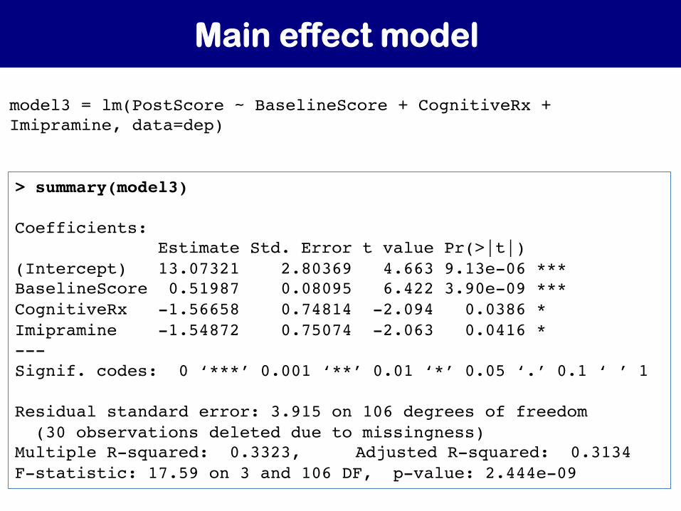
model3 = lm(PostScore ~ BaselineScore + CognitiveRx + Imipramine, data=dep)

> summary(model3)

Coefficients: Estimate Std. Error t value Pr(>|t|) (Intercept) 13.07321 2.80369 4.663 9.13e-06 ***BaselineScore 0.51987 0.08095 6.422 3.90e-09 ***CognitiveRx -1.56658 0.74814 -2.094 0.0386 * Imipramine -1.54872 0.75074 -2.063 0.0416 * ---Signif. codes: 0 ‘***’ 0.001 ‘**’ 0.01 ‘*’ 0.05 ‘.’ 0.1 ‘ ’ 1


Main effect model

model3 = lm(PostScore ~ BaselineScore + CognitiveRx + Imipramine + CognitiveRx:Imipramine, data=dep)

> summary(model3)

Coefficients: Estimate Std. Error t value Pr(>|t|) (Intercept) 19.8959 4.3582 4.565 1.36e-05 ***BaselineScore 0.5222 0.0798 6.543 2.25e-09 ***CognitiveRx -6.0970 2.3561 -2.588 0.0110 * Imipramine -6.1059 2.3695 -2.577 0.0114 * CognitiveRx:Imipramine 2.9875 1.4756 2.025 0.0455 *

---Signif. codes: 0 ‘***’ 0.001 ‘**’ 0.01 ‘*’ 0.05 ‘.’ 0.1 ‘ ’ 1


Interaction effect model

Summary

•  ANCOVA is a sta)s)cal method very useful for the analysis of change taking into account effects of covariate

•  In before-‐aMer experiments, ANCOVA is highly preferable to the percentage change from baselin analysis

•  Can implement Bayesian analysis in ANCOVA using R

tuanv.nguyen%% - garvan.org.au · analysis using r # read data into r wt = read.csv("~/google...

Documents