tuning fuzzy-logic controllerscdn.intechopen.com/pdfs-wm/34222.pdf · · 2018-04-06fuzzy logic...

17

Tuning Fuzzy-Logic Controllers

Trung-Kien Dao1 and Chih-Keng Chen2 1MICA Center, HUST - CNRS/UMI 2954 - Grenoble INP, Hanoi,

2Dayeh University, Changhua, 1Vietnam 2Taiwan

1. Introduction

The classical proportional-derivative (PD) control is relatively easy to design, but useful for

fast response controllers by combining proportional control and derivative control in parallel.

However, as PD control is linear, it is not able to be used to deal with non-linear plants. An

answer to this problem is fuzzy-logic control, which is also a model-free control scheme and

can be applied to systems where mathematical models cannot be obtained. Besides, natural

heuristic rules in linguistic expressions that reflect human experiences can be applied in the

control design, minimizing the design cost. Fuzzy-logic controllers (FLCs) are the control

systems based on a knowledge consisting of the so-called fuzzy IF-THEN rules.

This chapter is a discussion on using genetic algorithms (GAs) to tune the parameters of PD-like FLCs. Genetic algorithms are global search techniques modeled following the natural genetic mechanism to find approximate or exact solutions to optimization and search problems. In a GA, each parameter to be optimized is represented by a gene; moreover, each individual is characterized by a chromosome, which is actually a set of parameters awaiting optimization.

The remainder of this chapter is organized as follows. In Section 2, the optimization

technique for PD-like FLCs using GAs is explained. After that, two case studies are

presented and discussed in Sections 3 and 4, in which, the introduced technique is applied

for a bicycle roll-angle-tracking controller and an ESP controller, respectively. Finally,

concluding remarks are given in Section 5.

2. PD-Like fuzzy-logic controller and optimization

In a fuzzy IF-THEN rule, words can be characterized by continuous membership functions

(typically taking values from 0 to 1) representing the degree of truth of the statements. For

example, to stabilize the bicycle, the following fuzzy rule can be used:

IF the bicycle is leaning to the right AND the roll angle is increasing, THEN apply large steering torque to the right,

where the words right, increasing and large are characterized by corresponding membership functions. Similarly, more rules from human knowledge can be defined to make the control

www.intechopen.com

Fuzzy Logic – Controls, Concepts, Theories and Applications

352

system more precise. Combining these rules into a fuzzy system, a rule base is obtained, which is used by the fuzzy inference system (FIS), as shown in Fig. 1. Two common FIS used in the literature are that of Takagi and Sugeno (TS), and that of Mamdani. The difference of the two FIS is in the THEN clause, where TS method uses algebraic linear combination of fuzzy variables, while Mamdani method uses natural-language clauses.

Fig. 1. Basic configuration of fuzzy systems

By using FLC, one major advantage is that there is no need to beware of the exact plant model as when classical control schemes are used. In reality, the plant model is usually non-linear and difficult to specify exactly. Using FLC is a preferable approach to avoid this difficulty. However, in most of cases, the fuzzy membership functions are difficult to be effectively defined manually, and need to be tuned. One usual procedure to design a FLC is to approximately build the fuzzy rules and membership functions heuristically and subsequently use a certain optimization algorithm to tune the parameters.

Mamdani fuzzy inference system (FIS) is preferable in FLC instead of Takagi-Sugeno (TS) because of two reasons. First, since the IF-THEN rules of the Mamdani method are given in natural-language form, it is more intuitive to build the fuzzy rules so that the parameters can be determined later by using genetic algorithms. Secondly, the presentation of output membership functions by the TS method requires much more parameters, e.g. each THEN clause z = ax + by + c of a single rule has three parameters, which make the optimization become more complicated and computationally intensive. The distribution of the membership functions of each fuzzy variable of the FLCs discussed in this study can be determined by two parameters, a scaling factor and a deforming coefficient, using the Mamdani method; or six parameters in total for a two-input, one-output FLC.

To estimate the quality of an individual, a fitness function (objective function, or cost function) must be defined. A genetic algorithm starts by generating an initial population for the first generation; then, the quality of each individual is evaluated by using the fitness function. After one generation, only the advantageous individuals survive and reproduce to generate a new population for the next generation. By this process of selection from generation to generation, the quality of the offspring is improved in comparison with their ancestors.

During the creation of a new generation, a portion of the surviving individuals is recombined randomly via the so-called crossover and mutation operations, being adopted from natural evolution. The advantages of GAs over other searching algorithms are that they do not require any gradient information neither continuity assumption in searching for the best parameters, and that they can explore many characteristics at once, which is necessary when dealing with complex problems. For a complete introduction to GAs, the readers can refer to R.L. Haupt & S.E. Haupt (2004).

www.intechopen.com


353

The optimization procedure of FLC using GAs is presented in Fig. 2. To reduce the learning

efforts for GA computation to optimize the FLC, the scaling factors and deforming

coefficients are used. Each fuzzy input or output of the FLC is encoded by two numbers: a

scaling factor and a deforming coefficient. This method allows a standard PD-like two-

input, one-output FLC to be represented as a six-parameter optimization problem.

Fig. 2. Optimization of control parameters using GAs

The membership functions of a PD-like FLC are triangular, i.e.,

, ,

0, ,

( ) /( ), ,( )

( ) /( ), ,

0, .

a b c

x a

x a b a a x btri x

c x c b b x c

x c

< − − ≤ <=

− − ≤ < > (1)

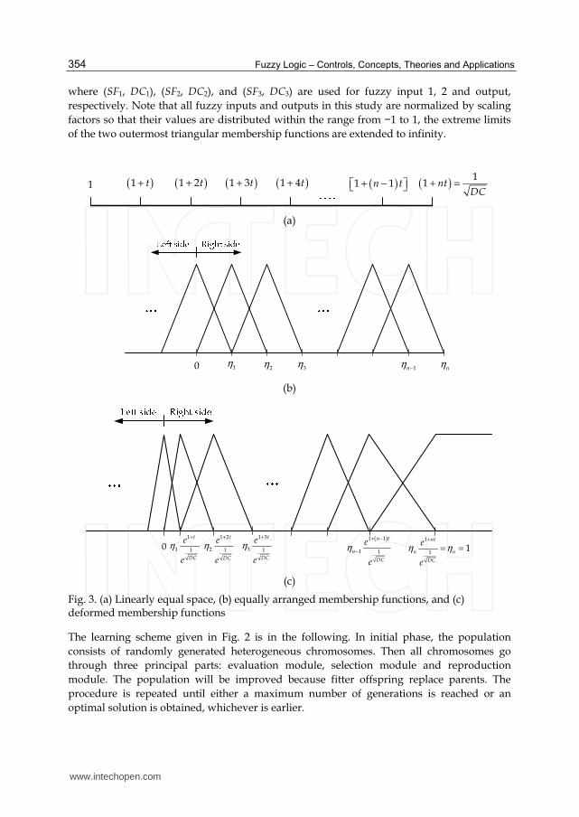
The coordinates a, b and c of the membership functions are determined from the

optimization process. The effect of the scaling factors is obtained by simply multiplying all

points of the universe of discourse of FLCs by the scaling factors. The deforming

coefficients, as illustrated in Fig. 3, are introduced to “deform” the membership functions so

that they are not equally distributed. Because the membership functions of a PD-like FLC

are symmetric with respect to the origin, it is only needed to calculate those on one side,

says the positive side, and then to take symmetrization to yield the other side. The

membership functions are deformed by multiplying all points of the universe of discourse

by the exponent of linearly equally space points within 1, 1 DC .

Let the number of points of the universe of discourse on the positive side, excluding the zero

origin, be n. The linear space is shown in Fig. 3a. By multiplying all points of the universe of

discourse by the exponent of this linear space and then rescaling by dividing to 1 DCe , the

equally distributed membership functions in Fig. 3b are transmuted into Fig. 3c without

changing the maximum limit ┟n. With the introduction of the scaling factors and deforming

coefficients, six parameters are needed to encode an FLC of two inputs and one output in

the form of a chromosome for GAs as follows

[ ]1 2 3 1 2 3 ,SF SF SF DC DC DC (2)

www.intechopen.com


354

where (SF1, DC1), (SF2, DC2), and (SF3, DC3) are used for fuzzy input 1, 2 and output,

respectively. Note that all fuzzy inputs and outputs in this study are normalized by scaling

factors so that their values are distributed within the range from −1 to 1, the extreme limits

of the two outermost triangular membership functions are extended to infinity.

1 ( )+ =1

1 ntDC

( )1 1n t + − ( )1 t+ ( )1 2t+ ( )1 3t+ ( )1 4t+

(a)

0 η1 η2 η3 ηnη −1n

(b)

0 η+1

1 1

t

DC

e

e

η+1 2

2 1

t

DC

e

e

η+1 3

3 1

t

DC

e

e

( )

η+ −

−

1 1

1 1

n t

n

DC

e

e

η η+

= =1

11

nt

n n

DC

e

e

(c)

Fig. 3. (a) Linearly equal space, (b) equally arranged membership functions, and (c) deformed membership functions

The learning scheme given in Fig. 2 is in the following. In initial phase, the population

consists of randomly generated heterogeneous chromosomes. Then all chromosomes go

through three principal parts: evaluation module, selection module and reproduction

module. The population will be improved because fitter offspring replace parents. The

procedure is repeated until either a maximum number of generations is reached or an

optimal solution is obtained, whichever is earlier.

www.intechopen.com


355

In the following of this chapter, two case studies are introduced to show the application of the PD-like FLCs and the control-parameter optimization technique in reality. In the first case, an FLC is used to establish a controller which helps a bicycle to follow a roll-angle command. In the second one, several FLCs are used in an ESP controller, which is designed to enhance vehicle maneuvers, especially in critical situations.

3. Case study: Bicycle roll-angle-tracking controller

As an unstable and underactuated system, the bicycle is control-challenging and can offer a

number of research interests in the area of mechanics and robot control. Control efforts for

stabilizing unmanned bicycles have also been addressed in previous studies. Yavin (1999)

dealt with the stabilization and control of a riderless bicycle by a pedaling torque, a

directional torque and a rotor mounted on the crossbar that generated a tilting torque.

Beznos et al. (1988) modeled a bicycle with gyroscopes that enabled the vehicle to stabilize

itself in an autonomous motion along a straight line as well as along a curve. In their study,

the stabilization unit consisted of two coupled gyroscopes spinning in opposite directions.

Han et al. (2001) derived a simple kinematic and dynamic formulation of an unmanned

electric bicycle. The controllability of the stabilization problem was also checked and a

control algorithm for self-stabilization of the vehicle with bounded wheel speed and

steering angle using non-linear control based on the sliding patch and stuck phenomena

was proposed.

Among studies relative to two-wheel-vehicle control, Sharp et al. (2004) presented a related

work on the roll-angle-tracking of motorcycles. A PID controller was used to generate the

steering torque based on the tracking error. In this section, a controller is introduced to

control the bicycle to follow a roll-angle command, where an FLC is used in the place of the

PID.

3.1 Control structure

Fig. 4 shows the roll-angle-tracking control structure that Sharp et al. (2004) used to control a

motorcycle. The steering torque is derived from the roll-angle error using a PID controller,

whose gains kP, kI and kD are speed-dependent. Their study has showed good results that the

steering torque of a two-wheeled vehicle can be directly controlled from the roll-angle error.

In this study, since PID controller is linear, it is replaced by a FLC in order to better deal

with the non-linearity of the bicycle. This gives the controller shown in Fig. 5.

Motorcycle┠ref e┠ τ outputs

┠ kD

kP

kI

d/dt

Vx

Fig. 4. Roll-angle-tracking controller for motorcycle (Sharp et al., 2005)

www.intechopen.com


356

The FLC used in this study has two inputs: the roll-angle tracking error e┠ = ┠ref – ┠, which is the difference between the desired roll angle and the actual one; and its change Δe┠. The controller generates appropriate control output which is the control torque τ to the steering fork. The FLC is PD-like since it requires two inputs, the error need to be minimized, and its variation, which are comparable to the proportional and derivative parts of a PD controller. Compared to the previous studies (Chen & T.S. Dao, 2006, 2007), the controller structure has been simplified so that only one FLC is used to generate the torque τ directly from the roll-angle error e┠, as shown in Fig. 5. Linguistic quantification used to specify a set of rules for this controller is characterized by the following three typical situations:

1. If e┠ is negative large (NL) and Δe┠ is NL, then τ is positive large (PL). This rule quantifies the situation wherein the desired roll-angle is much smaller than the actual one and the bicycle is falling to the right at a significant rate. Hence, one should steer the fork to the right more at a large positive angle to make the bicycle lean to the left.

2. If e┠ is zero (Z) and Δe┠ is Z, then τ is Z. This rule quantifies the situation wherein the bicycle is already in its proper position. No control effort is needed.

3. If e┠ is PL and Δe┠ is PL, then τ is NL. This rule quantifies the situation wherein the desired roll-angle is much larger than the actual one and the bicycle is falling to the left at a significant rate. Therefore, one should steer the fork to the left at a large angle to make the bicycle lean to the right.

Fig. 5. Roll-angle-tracking controller using FLC

eθ

eθ

Δ

Table 1. Rule base for roll-angle-tracking FLC

www.intechopen.com


357

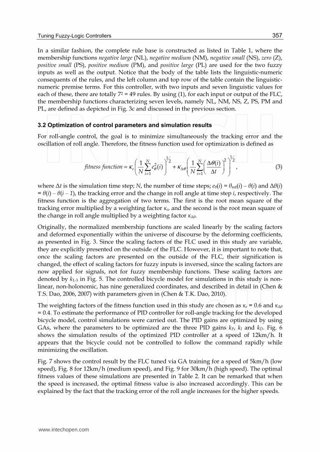
In a similar fashion, the complete rule base is constructed as listed in Table 1, where the membership functions negative large (NL), negative medium (NM), negative small (NS), zero (Z), positive small (PS), positive medium (PM), and positive large (PL) are used for the two fuzzy inputs as well as the output. Notice that the body of the table lists the linguistic-numeric consequents of the rules, and the left column and top row of the table contain the linguistic-numeric premise terms. For this controller, with two inputs and seven linguistic values for each of these, there are totally 72 = 49 rules. By using (1), for each input or output of the FLC, the membership functions characterizing seven levels, namely NL, NM, NS, Z, PS, PM and PL, are defined as depicted in Fig. 3c and discussed in the previous section.

3.2 Optimization of control parameters and simulation results

For roll-angle control, the goal is to minimize simultaneously the tracking error and the oscillation of roll angle. Therefore, the fitness function used for optimization is defined as

11 2 222

1 1

1 1 ( ) ( )

N N

ei i

ifitness function e i

N N tθ θ

θκ κΔ

= =

Δ = + Δ , (3)

where Δt is the simulation time step; N, the number of time steps; e┠(i) = ┠ref(i) – ┠(i) and Δ┠(i) = ┠(i) – ┠(i – 1), the tracking error and the change in roll angle at time step i, respectively. The fitness function is the aggregation of two terms. The first is the root mean square of the tracking error multiplied by a weighting factor κe, and the second is the root mean square of the change in roll angle multiplied by a weighting factor κΔ┠.

Originally, the normalized membership functions are scaled linearly by the scaling factors and deformed exponentially within the universe of discourse by the deforming coefficients, as presented in Fig. 3. Since the scaling factors of the FLC used in this study are variable, they are explicitly presented on the outside of the FLC. However, it is important to note that, once the scaling factors are presented on the outside of the FLC, their signification is changed, the effect of scaling factors for fuzzy inputs is inversed, since the scaling factors are now applied for signals, not for fuzzy membership functions. These scaling factors are denoted by k1-3 in Fig. 5. The controlled bicycle model for simulations in this study is non-linear, non-holonomic, has nine generalized coordinates, and described in detail in (Chen & T.S. Dao, 2006, 2007) with parameters given in (Chen & T.K. Dao, 2010).

The weighting factors of the fitness function used in this study are chosen as κe = 0.6 and κΔ┠ = 0.4. To estimate the performance of PID controller for roll-angle tracking for the developed bicycle model, control simulations were carried out. The PID gains are optimized by using GAs, where the parameters to be optimized are the three PID gains kP, kI and kD. Fig. 6 shows the simulation results of the optimized PID controller at a speed of 12km/h. It appears that the bicycle could not be controlled to follow the command rapidly while minimizing the oscillation.

Fig. 7 shows the control result by the FLC tuned via GA training for a speed of 5km/h (low speed), Fig. 8 for 12km/h (medium speed), and Fig. 9 for 30km/h (high speed). The optimal fitness values of these simulations are presented in Table 2. It can be remarked that when the speed is increased, the optimal fitness value is also increased accordingly. This can be explained by the fact that the tracking error of the roll angle increases for the higher speeds.

www.intechopen.com


358

0 2 4 6 8 10 12 14 16-15

-10

-5

0

5

10

15

Time (s)

Roll

angle

(deg)

Reference command

Response

Fig. 6. PID controller performance at normal speed (12km/h)

0 2 4 6 8 10 12 14 16-15

-10

-5

0

5

10

15

Time (s)

Roll

angle

(deg)

Reference command

Response

Fig. 7. Roll-angle-tracking performance at low speed (5km/h)

In comparison with the same control simulation but using PID controller in Fig. 6, it appears that the roll-angle tracking error is reduced when the bicycle is controlled by the FLC, as shown in Fig. 8. This is assured by the optimal value of fitness function of 0.0821 from the FLC, and 1.7153 from the PID controller for the same bicycle speed of 12km/h. By applying the optimized control parameters, the FLC can control the bicycle better than the PID controller does, which can be explained by the essential non-linear control properties. The FLC can control non-linear systems with a larger range of parameters.

www.intechopen.com


359

0 2 4 6 8 10 12 14 16-15

-10

-5

0

5

10

15

Time (s)

Roll

angle

(deg)

Reference command

Response

Fig. 8. Roll-angle-tracking performance at normal speed (12km/h)

0 2 4 6 8 10 12 14 16

-30

-20

-10

0

10

20

30

Time (s)

Roll

angle

(deg)

Reference command

Response

Fig. 9. Roll-angle-tracking performance at high speed (30km/h)

Controller Speed (km/h) Optimal fitness value

PID 12 1.7153

FLC 5 0.0430

FLC 12 0.0821

FLC 30 0.1378

Table 2. Optimal fitness values for simulations

www.intechopen.com


360

4. Case study: ESP controller

The Electronic Stability Program (ESP) is a vehicle dynamics control system that relies on a vehicle’s braking system to support the driver in critical driving situations. Since their landmark introduction of Bosch controller (Van Zanten et al., 1995), ESP systems have become popular in the automotive market. The general strategy of ESP systems is to define an indicator for the maneuverability of an automobile, from which the controller aims to enhance handling in extreme maneuvers by automatically controlling the brakes and the engine.

Satisfactory handling behavior is characterized by the fact that the vehicle correctly follows the desire of the driver; i.e., the vehicle yaw rate is accurately maintained according to the steering angle while concurrently remaining stable. The general concept of most ESP systems is primarily based on the sideslip angle, such as those presented by Van Zanten (2000); some systems regard also the vehicle yaw rate, for example the system developed by Kwak and Park (2001).

Mres

FB

FL

Mres

FB

FL

FB

FB

FB: brake forceFL: lateral tire forceMres: resulting moment

desired pathwithout ESP

with ESP

with ESP

without ESP

desired path

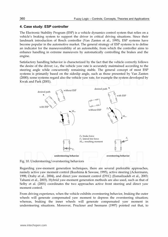
understeering behavior oversteering behavior

Fig. 10. Understeering/oversteering behaviors

Regarding yaw-moment generation techniques, there are several preferable approaches, namely active yaw moment control (Ikushima & Sawase, 1995), active steering (Ackermann, 1998; Oraby et al., 2004), and direct yaw moment control (DYC) (Esmailzadeh et al., 2003; Tahami et al., 2003). Hybrid yaw-moment generation methods are also used, such as that of Selby et al. (2001) coordinates the two approaches active front steering and direct yaw moment control.

From driving experience, when the vehicle exhibits oversteering behavior, braking the outer wheels will generate compensated yaw moment to depress the oversteering situation; whereas, braking the inner wheels will generate compensated yaw moment in understeering situations. Moreover, Pruckner and Seemann (1997) pointed out that, to

www.intechopen.com


361

stabilize the vehicle while braking, in case of understeering behavior, the main braking intervention should occur on the inner rear wheel. Rear braking force causes a primary yaw moment and a reduction in the rear lateral tire force. In case of oversteering behavior, the main braking force on the outer front wheel helps to stabilize the vehicle. The intervention produces a primary yaw moment and reduces the lateral tire force on the front side. These effects prevent critical oversteering driving situations, as shown in Fig. 10. For a more detailed description of ESP and controller principles, the readers can refer to Bosch (1999).

In this section, an ESP control approach based on an estimation of the desired yaw rate, considered to be the target yaw rate, which the vehicle should follow, is introduced. The fundamental idea regarding the estimated target yaw rate is to generate a compensated yaw moment which corrects the behaviors of the vehicle, thereby improving its handling and stability by using FLCs. When the compensated yaw moment is generated, the system also avoids the vehicle sideslip angle to prevent a counter-effect wherein this angle is increased to the limit. The distribution of braking forces on all wheels instead of two front wheels has two advantages. The first advantage is that the controller can generate larger yaw moment in severe situations. The second one is to make the vehicle more stable when the controller is activated. By distributing braking forces on all wheels, the controller can deal with more situations.

4.1 Control structure

An ESP system is developed to correct the yaw rate of a vehicle, especially in critical situations, so that the vehicle responds normally to the driver’s desire. This goal is achieved by estimating a corrective yaw moment, referred to as a compensated yaw moment, and generating the corresponding yaw moment to the vehicle by controlling the braking system, so that the vehicle can dependably respond to the driver’s maneuvers in critical situations. This estimation consists of two components, one based on the steering and the other on the sideslip angle.

Fig. 11. Overall ESP control structure

The overall control structure is depicted in Fig. 11. As previously mentioned, the compensated yaw moment is combined from two separately estimated components, Mzδ and Mz┚. From the estimated compensated yaw moment and the steering orientation, the reference pressure generator determines which wheels to brake and the braking pressures to be applied to each. A closed-loop pressure controller manipulates the EHB (electro-hydraulic brake) hydraulic pressures on the four wheels by following the reference pressures.

www.intechopen.com


362

4.1.1 Steering-based compensated yaw moment

During operation, the yaw rate of a vehicle should be proportional to the steering angle that

the driver makes with the steering wheel so that the time response of the yaw rate has the

same shape as that of the steering angle. The goal of the ESP system is to assure that this

criterion is achieved, especially in extreme situations.

From the theory of vehicle dynamics, the following equation can be derived:

2 2

1 122

1 2 1 22 ( ) 2 ( )

x g xz

x x

r g g r

V k V

ml V ml Vll

C l l k k C l lα α

δ δΩ ≈ =

− −+ +

. (4)

where Ωz is the vehicle yaw rate, Vx is the longitudinal speed in coordinates fixed to the

vehicle, m is the vehicle mass, l1 and l2 are the distances from the front and rear axles,

respectively, to the center of gravity, C┙r is the cornering stiffness of the rear tire, kg is the

gear ratio from the steering wheel to the front wheels, and δ is the angle of the steering

wheel. The following two magnitudes are now defined as

21

g

lk

k= and 1

21 22 ( )g r

mlk

k C l lα

=+

; (5)

thus, equation (4) can be simply denoted as

2

1 2

.xz

x

V

k k V

δΩ ≈

− (6)

It is noticed that every magnitudes involved in equation (5) are constants taken from the

configuration of a vehicle; thus, k1 and k2 are also constants. In consequence, in equation (6),

the steady-state yaw rate Ωz is a function of the longitudinal speed Vx and the steering angle

δ. It should be emphasized that this yaw rate does not depend on the friction coefficient μ. In

this ESP system, the objective is to control the vehicle so that its yaw rate follows the

reference yaw rate generated by this equation.

c

Fig. 12. Steering-based compensated yaw moment

Once the reference yaw rate is available, the maneuverability situation, understeering or

oversteering, can be determined by comparing the reference yaw rate to the actual one

measured from the yaw-rate sensor. When cornering, understeering situation is identified if

the absolute value of the real yaw rate is smaller than the desired one, and vice versa.

www.intechopen.com


363

Oversteering situation is identified if the absolute value of the real yaw rate is larger than

the desired one. The yaw-rate error, defined as

z z zrefeΩ = Ω − Ω , (7)

is used to generate the compensated yaw moment by a PD-like fuzzy logic control (FLC),

as shown in Fig. 12. The FLC requires two inputs, namely the yaw-rate error and its

variation, and one output, the compensated yaw moment. The ESP controller must

generate a moment corresponding to the compensated yaw moment so that the vehicle

yaw rate follows the steering angle correctly, thus implying that the vehicle

maneuverability is guaranteed.

4.1.2 Sideslip-angle-based compensated yaw moment

Abusing the steering to estimate the compensated yaw moment might make the vehicle

go out of control when the sideslip angle ┚ (angle between the vehicle’s moving direction

and the direction towards which it is pointing) becomes too high. To prevent this

situation, when ┚ exceeds a certain predefined value ┚0, the system will generate another

compensated yaw moment in such a manner that the sideslip angle has the tendency to

decrease. This can be achieved by another PD-like FLC as shown in Fig. 13. After Van

Zanten (2000), during normal driving, average drivers will not exceed sideslip angles of

±2°. Beyond this value, the driver has no experience. In this controller, the value of ┚0 is

chosen to be 1.5°, which is the value that the sideslip-angle-based compensated yaw

moment starts having effect.

Fig. 13. Sideslip-angle-based compensated yaw moment

Note that for implementing in real cars, there are several methods for estimating the sideslip

angle of a vehicle. Two common approaches are the vehicle model observer and the pseudo-

integral. The former estimates the sideslip angle based on a vehicle model, which is

generally robust against sensor errors, yet sensitive to changes in condition and

disturbances; whereas, the latter estimates the sideslip by taking integration of

( ) /x x zy V Vβ β= − − Ω , where y is lateral acceleration, Vx is vehicle speed, and Ωz is vehicle

yaw rate, which is robust against changes in road friction and disturbances. However,

stabilization should be applied in the latter to minimize the cumulative integral error.

Nishio et al. (2001) developed an estimation method using a combination of the vehicle

model observer and the pseudo-integral. This method is robust against sensor error as well

as changes in road friction and operational disturbances.

www.intechopen.com


364

The steering-based compensated yaw moment Mzδ and the sideslip-angle-based one Mz┚ are later combined as Mz. The activator is a logical block producing 1 or 0, depending on whether ┚ is greater than ┚0. Thus, by the multiplication operator, the effect of the activator is to enable or disable the sideslip-angle-based branch regarding whether ┚ exceeds ┚0.

4.1.3 Braking-pressure control

As previously discussed, the distribution of the braking pressure aims to generate the yaw moment effectively while keeping the vehicle stable during braking. In understeering situation, the inner rear wheel is braked primarily. If the desired yaw moment is large, the inner front wheel will also be braked secondarily to generate a supplementary yaw moment and stabilize the vehicle. In oversteering situation, the outer front wheel is braked primarily, and the outer rear wheel is braked secondarily if large yaw moment is required. The braking-pressure distribution is summarized in Table 3.

Understeering Oversteering

Turn left (δ > 0) Turn right (δ < 0) Turn left (δ > 0) Turn right (δ < 0)

Small Mz Large Mz Small Mz Large Mz Small Mz Large Mz Small Mz Large Mz

FL Secondary Primary Primary

FR Secondary Primary Primary

RL Primary Primary Secondary

RR Primary Primary Secondary

Table 3. Braking-pressure distribution

Fig. 14. Structure of pressure controller

The pressure is controlled by a closed-loop control structure using an FLC, as shown in Fig.

14. On the basis of the error between the actual-pressure measurement and the reference

pressure, and the variation of the error itself, the FLC generates the control signal uc. The

values of uc are in the range from −1 to 1, corresponding to the openness of the inlet and

outlet valves of the EHB system explicated in the previous section. Regarding the sign and

value of uc, the actuator switch opens or closes the inlet and outlet valves.

4.2 Optimization of control parameters and simulation results

It is clear that the components of this controller, such as the reference yaw-rate estimator, the compensated yaw-moment generators, and the pressure controller, can be optimized separately. Optimizing each component individually reduces the complexity in formulating the problem and avoids unnecessary combinatory operations among unrelated genes

www.intechopen.com


365

caused by the interaction effect between components, thereby saving much computational time. However, it is important to note that the order for optimizing these components is not totally arbitrary, due to their dependence. For example, optimizing the pressure controller requires that the pressure model be built and parameters be tuned a priori.

First, the reference yaw-rate generator can be isolated from the whole control model and tuned independently, since their parameters are tuned to fit data measured from experiments. After that, the pressure controller can be optimized. Once these three components are completed, the next step is optimizing the steering-based compensated yaw-moment generator, and finally the sideslip-based compensated yaw-moment generator to complete the optimization procedure. The optimal values of control parameters used in this study are presented in Table 4.

Component Parameter Value

Steering-based FLC Scaling factors [ ]0.108 0.008 15.106

Deforming coefficients [ ]0.704 0.660 0.173

Sideslip-angle based FLC Scaling factors [ ]1.473 0.253 19.593

Deforming coefficients [ ]0.193 0.694 0.360

Table 4. Optimal control parameters for ESP

0 1 2 3 4 5

-50

0

50

100

Time (s)

Ste

ering a

ngle

(deg)

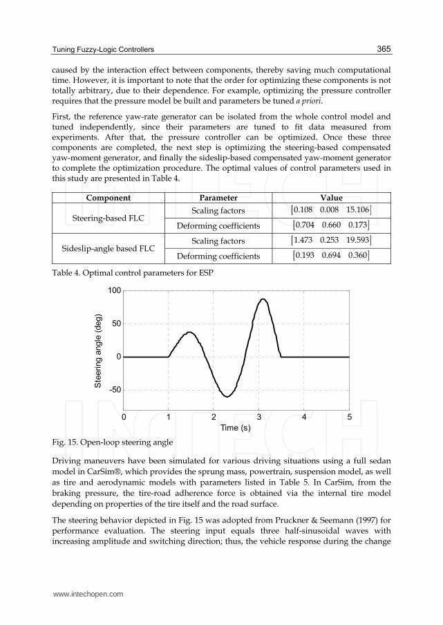
Fig. 15. Open-loop steering angle

Driving maneuvers have been simulated for various driving situations using a full sedan

model in CarSim®, which provides the sprung mass, powertrain, suspension model, as well

as tire and aerodynamic models with parameters listed in Table 5. In CarSim, from the

braking pressure, the tire-road adherence force is obtained via the internal tire model

depending on properties of the tire itself and the road surface.

The steering behavior depicted in Fig. 15 was adopted from Pruckner & Seemann (1997) for

performance evaluation. The steering input equals three half-sinusoidal waves with increasing amplitude and switching direction; thus, the vehicle response during the change

www.intechopen.com


366

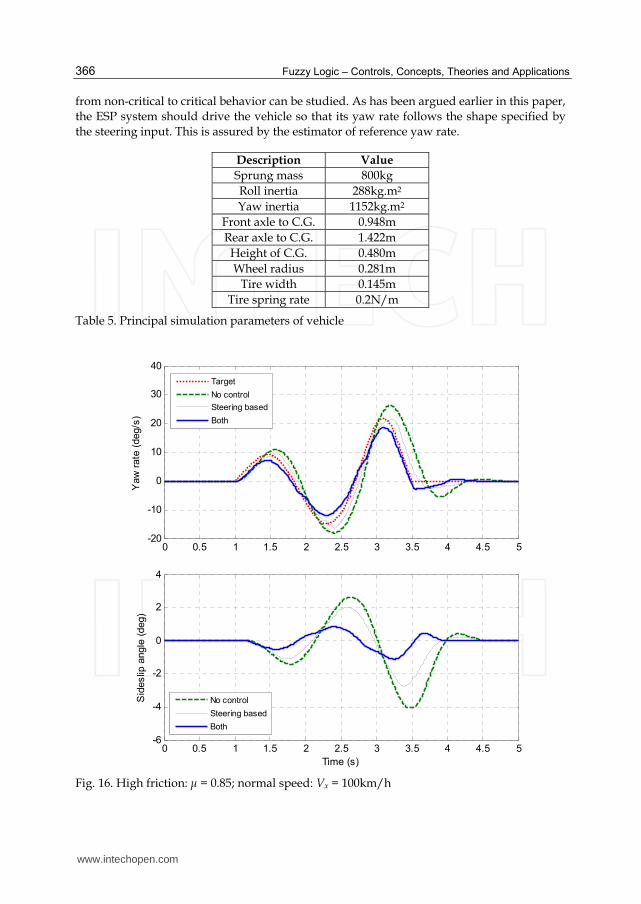
from non-critical to critical behavior can be studied. As has been argued earlier in this paper, the ESP system should drive the vehicle so that its yaw rate follows the shape specified by the steering input. This is assured by the estimator of reference yaw rate.

Description Value

Sprung mass 800kg

Roll inertia 288kg.m2

Yaw inertia 1152kg.m2

Front axle to C.G. 0.948m

Rear axle to C.G. 1.422m

Height of C.G. 0.480m

Wheel radius 0.281m

Tire width 0.145m

Tire spring rate 0.2N/m

Table 5. Principal simulation parameters of vehicle

0 0.5 1 1.5 2 2.5 3 3.5 4 4.5 5-20

-10

0

10

20

30

40

Yaw

rate

(deg/s

)

Target

No control

Steering based

Both

0 0.5 1 1.5 2 2.5 3 3.5 4 4.5 5-6

-4

-2

0

2

4

Time (s)

Sid

eslip

angle

(deg)

No control

Steering based

Both

Fig. 16. High friction: μ = 0.85; normal speed: Vx = 100km/h

www.intechopen.com


367

After tuning the controller by using GAs with mutation rate of 0.1, crossover rate of 0.8,

population size of 20, maximal number of generations of 50, and randomly generated initial

population, simulations for four cases with different road frictions and speeds were

conducted. The simulation results of which are shown in figures from 13 to 16. The first

simulation (Fig. 16) focused on high-friction and normal-speed conditions to determine how

the performance of a vehicle can be improved in non-critical situations. Next, the vehicle

behavior and controller performance were examined for three different critical situations,

namely high speed on high-friction surfaces (Fig. 17), high speed on normal-friction surfaces

(Fig. 18), and normal speed on very low-friction surfaces (Fig. 19). In each case, three trials

were considered: the first, without the ESP controller (dashed lines); the second, with only the

steering-based compensated yaw moment enabled (thin solid lines); the third, with both

steering-based and sideslip-angle-based compensated yaw moments taken into account (thick

solid lines). The target yaw rates (dotted lines) are shown in yaw-rate plots for reference.

-20

-10

0

10

20

30

40

50

Yaw

rate

(deg/s

)

Target

No control

Steering based

Both

0 0.5 1 1.5 2 2.5 3 3.5 4 4.5 5

-15

-10

-5

0

5

Time (s)

Sid

eslip

angle

(deg)

No control

Steering based

Both

Fig. 17. High friction: μ = 0.85; high speed: Vx = 180km/h

www.intechopen.com


368

First, a simulation was done for a highly maneuverable case characterized by high friction

and normal speed. The first plot in Fig. 16 indicates that without the ESP controller, the

vehicle was already following the steering target fairly well. However, a better result can

still be obtained with the ESP system enabled. The second plot shows that the sideslip angle

was significantly reduced with the use of the compensated yaw moment.

The second simulation was done for conditions characterized by high friction and high

speed, the results of which are shown in Fig. 17. Without the ESP controller, the vehicle

went out of control when the steering began to become critical (at 3.2 sec). The ESP

controller successfully drove the vehicle following the steering target.

The third simulation was done for a case characterized by medium friction and high speed,

the results of which are shown in Fig. 18. Without the ESP controller, the vehicle went out of

control even when the steering was non-critical (at 2.2 sec). The ESP controller performed

quite well in this case while keeping the vehicle yaw rate almost coincidental with the

steering target.

-60

-40

-20

0

20

Yaw

rate

(deg/s

)

Target

No control

Steering based

Both

0 0.5 1 1.5 2 2.5 3 3.5 4 4.5 5-5

0

5

10

15

Time (s)

Sid

eslip

angle

(deg)

No control

Steering based

Both

Fig. 18. Medium friction: μ = 0.5; high speed: Vx = 180km/h

www.intechopen.com


369

The last simulation case, the results of which are shown in Fig. 19, was for a very low-

friction condition, corresponding to driving on snow-covered or icy surfaces. In this

emergency situation, even with the ESP controller, the tracking for critical-steering

maneuvering was not really good, the yaw rate drew much closer to the steering target and

the sideslip angle being kept under the specified range (two degrees).

0 0.5 1 1.5 2 2.5 3 3.5 4 4.5 5-30

-20

-10

0

10

20

Yaw

rate

(deg/s

)

Target

No control

Steering based

Both

0 0.5 1 1.5 2 2.5 3 3.5 4 4.5 5-10

-5

0

5

10

Time (s)

Sid

eslip

angle

(deg)

No control

Steering based

Both

Fig. 19. Low friction: μ = 0.2; normal speed: Vx = 100km/h

www.intechopen.com


370

5. Conclusion

In this chapter, an optimization technique was introduced to tune the parameters of PD-like fuzzy-logic controllers. The key point is to parameterize each input and output of a FLC by a scaling factor and a deforming coefficient. In this way, the FLC can be tuned quantitatively by different optimization algorithms, among which the genetic algorithms introduced are a preferable choice. The design of PD-like FLCs is as simple as a PID, as it does not require a mathematic model of the control plant, even a simple one. However, these FLCs gain over PID controllers by the non-linear properties, thus, are widely used in non-linear control problems where plant models are difficult to obtain mathematically.

From the introduced technique, two case studies were presented and discussed. In the first case, a bicycle roll-angle-tracking controller was an attempt to adapt the study of Sharp et al. for motorcycle to control the bicycle, where an FLC was used instead of a PID so that the system non-linearity was better dealt. Simulation results indicated that the bicycle can follow roll-angle commands with small error. In the second case, after the FLCs were optimized, simulations using the ESP system were conducted under different driving conditions. In normal conditions, the controller could still improve the maneuverability to achieve better performance. In high speed conditions, the vehicle was controlled to follow the desired yaw rate with small sideslip angle. In very low friction conditions, although the controller could not control the vehicle back to the normal condition, the yaw rate drew much closer to the steering target and the sideslip angle was kept to be in the specified range. The results indicate that, with the help of proposed ESP control scheme, a vehicle can follow a steering behavior in critical cases while maintaining a small sideslip angle.

The PD-like FLCs can be widely applied in reality due to several advantages. First, the control design is simple, without the need to develop a dynamic model for the control plan. This is because FLC is a model-free control scheme. Second, human experience can be used straightforwardly in the design of the controller. The designer can describe the system behavior with simple IF-THEN rules. All the optimization efforts of control performance are then endorsed by the adjustment process of the fuzzy membership functions. This process has also strengths and weaknesses. While the easily adjustable membership functions give the designers a lot of chance to affect the control performance, there is no general analytical technique. This study is an effort to address this problem by parameterizing the fuzzy membership functions with scaling factors and deforming coefficients, which can be used as control parameters in the optimization. Among many optimization methods, the GA approach introduced in this study is a good choice as it is a general optimization method, which is able to search for the global optimum of knowledge-free problems.

6. Acknowledgement

The work was supported by the National Science Council in Taiwan, Republic of China, under the projects numbered NSC 96-2221-E-212-027 and NSC 97-2221-E-212-007, and by MICA Center, HUST - CNRS/UMI 2954 - Grenoble INP.

7. References

Ackermann, J. (1998). Active steering for better safety, handling and comfort, Proceedings of

Advances in Vehicle Control and Safety, Amiens, France, pp. 1-10

www.intechopen.com


371

Beznos, A.V.; Formal’sky, A.M.; Gurfinkel, E.V.; Jicharev, D.N.; Lensky, A.V.; Savitsky, K.V.

& Tchesalin, L.S. (1988). Control of autonomous motion of two-wheel bicycle with

gyroscopic stabilisation, Proc. of IEEE Int. Conf. on Robotics and Automation, Leuven,

Belgium, Vol. 3, pp. 2670-2675

Bosch (1999). Driving-Safety Systems, 2nd ed., Stuttgart: Robert Bosch GmbH, Society of

Automotive Engineers

Chen, C.K. & Dao, T.S. (2006). Fuzzy control for equilibrium and roll-angle tracking of an

unmanned bicycle, Multibody System Dynamics, Vol. 15, pp. 325-350

Chen, C.K. & Dao, T.S. (2007). Genetic fuzzy control for path-tracking of an autonomous

robotic bicycle, J. of System Design and Dynamics, vol. 1, pp. 536-547

Chen, C.K. & Dao, T.K. (2010). Speed-adaptive roll-angle-tracking control of an unmanned

bicycle using fuzzy logic, Vehicle System Dynamics (Special Issue: Selected Papers from the 22nd International Congress of Theoretical and Applied Mechanics, Adelaide, 24–29

August 2008), Vol. 48, pp. 133-147. DOI: 10.1080/00423110903085872

Esmailzadeh, E.; Goodarzi, A. & Vossoughi, G.R. (2003). Optimal yaw moment control law

for improved vehicle handling, Mechatronics, Vol. 13, No. 7, pp. 659-675

Han, S.; Han, J. & Ham, W. (2001). Control algorithm for stabilization of tilt angle of

unmanned electric bicycle, Trans. on Control, Automation and Systems Engineering,

Vol. 3, pp. 176-180

Haupt, R.L. & Haupt, S.E. (2004). Practical Genetic Algorithm, 2nd ed., John Wiley & Sons, Inc.

Ikushima, Y. & Sawase, K. (1995). A study on the effects of the active yaw moment control,

SAE Technical Paper Series, No. 950303

Kwak, B. & Park, Y. (2001). Robust vehicle stability controller based on multiple sliding

mode control, SAE Technical Paper Series, No. 2001-01-1060

Nishio, A.; Tozu, K.; Yamaguchi, H.; Asano, K. & Amano, Y. (2001). Development of vehicle

stability control system based on vehicle sideslip angle estimation, SAE

Transactions, Vol. 110, No. 6, pp. 115-122

Oraby, W.A.H.; El-Demerdash, S.M.; Selim, A.M.; Faizz, A. & Crolla, D.A. (2004).

Improvement of vehicle lateral dynamics by active front steering control, SAE

Technical Paper Series, No. 2004-01-2081

Pruckner, A. & Seemann, M. (1997). Analysis of dynamic driving control systems (DDC) on

a full vehicle model in ADAMS, Institut fur Kraftfahrwesen Aachen

Selby, M.; Manning, W.J.; Brown, M.D. & Crolla, D.A. (2001). A coordination approach for

DYC and active front steering, SAE Transactions, vol. 110, no. 6, pp. 1411-1417

Sharp, R.S.; Evangelou, S. & Limebeer, D.J.N. (2004). Advances in the modelling of

motorcycle dynamics, Multibody System Dynamics, Vol. 12, pp. 251-283

Tahami, F.; Kazemi, R. & Farhanghi, S. (2003). Direct yaw control of an all-wheel-drive EV

based on fuzzy logic and neural networks, SAE Technical Paper Series, No. 2003-01-

0956

Van Zanten, A.T.; Erhardt, R. & Pfaff, G. (1995). VDC, the vehicle dynamics control system

of Bosch, SAE Technical Paper Series, No. 950759

Van Zanten, A.T. (2000). Bosch ESP systems: 5 years of experience, SAE Transactions, Vol.

109, No. 7, pp. 428-436

www.intechopen.com


372

Yavin, Y. (1999). Stabilization and control of the motion of an autonomous bicycle by using a

rotor for the tilting moment, Computer Methods in Applied Mechanics and Engineering,

Vol. 178, pp. 233-243

www.intechopen.com

Fuzzy Logic - Controls, Concepts, Theories and ApplicationsEdited by Prof. Elmer Dadios

ISBN 978-953-51-0396-7Hard cover, 428 pagesPublisher InTechPublished online 28, March, 2012Published in print edition March, 2012

InTech EuropeUniversity Campus STeP Ri Slavka Krautzeka 83/A 51000 Rijeka, Croatia Phone: +385 (51) 770 447 Fax: +385 (51) 686 166www.intechopen.com

InTech ChinaUnit 405, Office Block, Hotel Equatorial Shanghai No.65, Yan An Road (West), Shanghai, 200040, China

Phone: +86-21-62489820 Fax: +86-21-62489821

This book introduces new concepts and theories of Fuzzy Logic Control for the application and development ofrobotics and intelligent machines. The book consists of nineteen chapters categorized into 1) Robotics andElectrical Machines 2) Intelligent Control Systems with various applications, and 3) New Fuzzy Logic Conceptsand Theories. The intended readers of this book are engineers, researchers, and graduate students interestedin fuzzy logic control systems.

How to referenceIn order to correctly reference this scholarly work, feel free to copy and paste the following:

Trung-Kien Dao and Chih-Keng Chen (2012). Tuning Fuzzy-Logic Controllers, Fuzzy Logic - Controls,Concepts, Theories and Applications, Prof. Elmer Dadios (Ed.), ISBN: 978-953-51-0396-7, InTech, Availablefrom: http://www.intechopen.com/books/fuzzy-logic-controls-concepts-theories-and-applications/tuning-fuzzy-logic-controllers

tuning fuzzy-logic controllerscdn.intechopen.com/pdfs-wm/34222.pdf · · 2018-04-06fuzzy logic...

Documents