D R A G I C A VA S I L E S K A A N D G E R H A R D K L I M E C K

TUNNELING

QUANTUM EFFECTS

• Quantum-mechanical space quantization• Tunneling• Quantum Interference

In all but the smallest devices quantum-mechanical space quantization effects and tunneling play dominant role and they can be captured with quantum correction models

Quantum interference dominates the operation of resonant tunneling diodes and fully quantum transport approaches are needed to treat this device.

TREATMENT OF TUNNELING

• WKB Approximation• Transfer Matrix Approach

• Piece-Wise Constant Potential Barrier Approximation• Piece-Wise Linear Potential Barrier Approximations

WENTZEL-KRAMERS-BRILLOUIN(WKB) APPROXIMATION

IMPORTANT APPLICATIONS IN WHICH WKB APPROXIMATION IS USED

• Tunneling Breakdown in normal diodes (reverse biased diode)

• Tunnel (Esaki) diode (forward + reverse bias)• Scanning Tunneling Microscope• Gate Leakage in MOSFET Devices

A. BREAKDOWN MECHANISMS IN A DIODE

• Junction breakdown can be due to:

� tunneling breakdown

� avalanche breakdown

• One can determine which mechanism is responsible for the

breakdown based on the value of the breakdown voltage VBD :

� VBD < 4Eg/q →→→→ tunneling breakdown

� VBD > 6Eg/q →→→→ avalanche breakdown

� 4Eg/q < VBD < 6Eg/q →→→→ both tunneling and

avalanche mechanisms are responsible

• Tunneling breakdown occurs in heavily-doped pn-

junctions in which the depletion region width W is about

10 nm.

W

EF

EC

EV

Zero-bias band diagram: Forward-bias band diagram:

W

EFn

EC

EV

EFp

EFn

EC

EV

EF

p

Reverse-bias band diagram: • Tunneling current (obtained by

using WKB approximation):

Fcr � average electric field in

the junction

• The critical voltage for

tunneling breakdown, VBR, is

estimated from:

• With T�, Eg� and It� .

−

π=

cr

g

g

crt

qF

Em

E

VAFqmI

�� 3

24exp

4

22/3*

2/122

3*

SBRt IVI 10)( ∝

B. TUNNEL (ESAKI) DIODE

Nobel Prize in Physics 1973

Leo Esaki

(ESAKI) TUNNEL DIODE (TD)

• Simplest tunneling device• Heavily-doped pn junction

• Leads to overlap of conduction and valence bands

• Carriers are able to tunnel inter-band• Tunneling goes exponentially with tunneling distance

• Requires junction to be abrupt

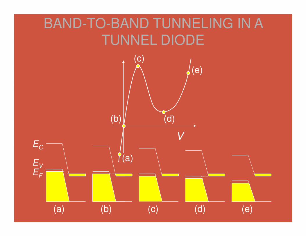
BAND-TO-BAND TUNNELING IN A TUNNEL DIODE

EC

EV

EF

V

(a)

(b)

(c)

(d)

(e)

(a) (b) (c) (d) (e)

FIGURES OF MERIT

V

Peak current

100 kA/cm2Peak-to-Valley Ratio (PVR)

DIRECT VS. INDIRECT TUNNELING

Direct Indirect

Indirect materials require phonons to tunnel, thus reducing the probability of a tunneling event

C. SCANNING TUNNELING MICROSCOPE

D. WKB APPROXIMATION EXPLAINED

• The Wentzel-Kramers-Brillouin (WKB) approximation is a “semiclassical calculation” in quantum mechanics in which the wavefunction is assumed an exponential function with amplitude and phase that slowly varies compared to the de Broglie wavelength, λ, and is then semiclassically expanded

• While Wentzel, Kramers and Brillouin developed this approach in 1926, earlier in 1923 Harold Jeffreys had already developed a more general method of approximating linear, second-order differential equations (the Schrodinger equation is a linear second order differential equation)

WKB APPROXIMATION EXPLAINED, CONT’D

• While technically this is an “Approximate Method” not an “Exact solution” to the Schrodinger equation, it is very close to simple plane wave solutions that we discussed while describing transmission coefficient calculation in piece-wise constant potential barriers

• The WKB method is most often applied to 1D problems but can be applied to 3D Spherically Symmetric problems as well (see Bohm 1951)

• The WKB approximation is especially useful in deriving the tunnel current in a tunnel diode

BASIC IDEA OF THE METHOD

• The WKB approximation states that since in a constant potential, the wavefunction solutions of the Schrodinger equation are of the form of simple plane waves, then

• Now, if the potential U=U(x) changes slowly with x, the solution of the Schrodinger equation can also be written of the general form

where φ(x)=xk(x). - For the constant potential case, φ(x)=±kx so the phase changes linearly with x- In a slowly varying potential φ(x) should vary slowly from the linear case ±kx

2

2 ( )( ) , 2 /ikx m E Ux Ae kψ π λ± −

= = =�

( )( ) i xx Ae

φψ =

BASIC IDEA OF THE METHOD, CONT’D

• For the two cases, E>U and E<U, let k(x) be defined as (so we only have to solve the problem once)

2

2

2 ( ( ))( ) , ( )

2 ( ( ) )( ) ( ), ( )

m E U xk x E U x

m U x Ek x i i x E U xκ

−= >

−= − = − <

�

�

WENTZEL-KRAMERS-BRILLOUIN (WKB) APPROXIMATION

• Starting from the 1D Schrödinger equation

• And substituting the general solution for slowly-varying potentials, one gets the following differential equation

2 2

2( ) ( ) ( ) ( )

2x U x x E x

m xψ ψ ψ

∂− + =

∂

�

222

2( ) 0i k x

x x

φ φ∂ ∂ − + =

∂ ∂

WENTZEL-KRAMERS-BRILLOUIN (WKB) APPROXIMATION

• The WKB approximation assumes that the potentials are slowly varying in space

• Then the 0th order approximation assumes

2

00 02

0

0, ( ) ( ) ( )

( ) exp ( )

k x x k x dx Cx x

x i k x dx C

φφφ

ψ

∂∂= = ± → = ± +

∂ ∂

→ = ± +

∫

∫

Wentzel-Kramers-Brillouin (WKB) Approximation

• If a higher order solution is required, then we solve

• Then the 1th order approximation assumes

22 22 2

2 2( ) 0 ( )i k x k x i

x x x x

φ φ φ φ∂ ∂ ∂ ∂ − + = → = ± +

∂ ∂ ∂ ∂

2

2

1

( )

( ) exp ( )

kk x i

x x

kx i k x i dx C

x

φ

ψ

∂ ∂= ± ±

∂ ∂

∂→ = ± ± +

∂ ∫

Wentzel-Kramers-Brillouin (WKB) Approximation

1. In order to apply the WKB approximation we only need to know the shape of the potential since

2. For slowly varying U(x) the first order and the zero order approximation give almost the same result as

2

1( ) ( ) ( ) ( ) exp ( )k

U x k x x x k x i dx Cx

φ ψ ∂

→ → → = ± ± + ∂

∫

2( ) ( )k x k xx

∂<<

∂

Wentzel-Kramers-Brillouin (WKB) Approximation

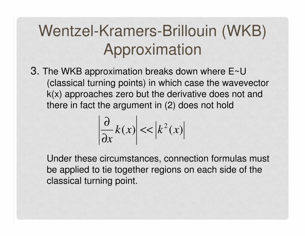
3. The WKB approximation breaks down where E~U (classical turning points) in which case the wavevector k(x) approaches zero but the derivative does not and there in fact the argument in (2) does not hold

Under these circumstances, connection formulas must be applied to tie together regions on each side of the classical turning point.

2( ) ( )k x k xx

∂<<

∂

E. EXAMPLE: GATE LEAKAGEgate leakage

tunnelling current

GATE LEAKAGE

� For sub-micrometer devices, due to smaller oxide thickness, there is significant conductance being measured on the gate contact. The finite gate current gives rise to the following effects:

� Negative => degradation in the device operating characteristics with time due to oxide charging; larger off-state power dissipation

� Positive => non-volatile memories utilize the gate current to program and erase charge on the “floating contact” – FLASH, FLOTOX, EEPROM

� There are two different types of conduction mechanisms to the insulator layer:

� Tunneling: Fowler-Nordheim or direct tunneling process

� Hot-carrier injection: lucky electron model or Concannon model

Electron is emitted into the oxide when it gains sufficient energy to overcome the insulator/semicon-ductor barrier.

• Similar to the lucky electron model, but assumes non-Maxwellian high energy tail on the distribution function.

• Requires solution of the energy balance equation for carrier temperature.

TUNNELING CURRENTS

� Three types of tunneling processes are schematically shown below(courtesy of D. K. Schroder)

• For tox ≥ 40 Å, Fowler-Nordheim (FN) tunneling dominates• For tox < 40 Å, direct tunneling becomes important• Idir > IFN at a given Vox when direct tunneling active• For given electric field: - IFN independent of oxide thickness

- Idir depends on oxide thickness

φφφφB Vox > φφφφB

Vox = φφφφB

Vox < φφφφB

FN FN/Direct Direct

tox

φφφφB Vox > φφφφB

Vox = φφφφB

Vox < φφφφB

FN FN/Direct Direct

tox

SIGNIFICANCE OF GATE LEAKAGE

10-16

10-14

10-12

10-10

10-8

10-6

10-4

0 50 100 150 200 250

Cu

rren

t (A

/µµ µµm

)

Technology Generation (nm)

Ion

IG

Ioff

� As oxide thickness decreases, the gate current becomes more important. It eventually dominates the off-state leakage current (ID at VG = 0 V)

� The drain current ID as a function of technology generation is shown below (courtesy of D. K. Schroder)

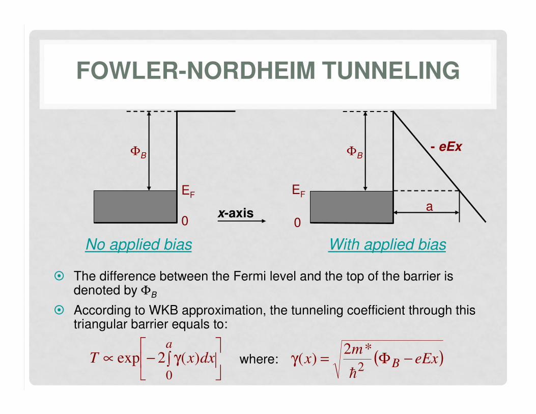
FOWLER-NORDHEIM TUNNELING

0

EF

ΦB

0

EF

ΦB

a

No applied bias With applied bias

- eEx

x-axis

� The difference between the Fermi level and the top of the barrier is denoted by ΦB

� According to WKB approximation, the tunneling coefficient through this triangular barrier equals to:

∫ γ−∝a

dxxT0

)(2exp where: ( )eExm

x B −Φ=γ2

*2)(

�

EZ

W

z

V(z)

zEG

EG-Ez

W

EZ

W

z

V(z)

zEG

EG-Ez

W

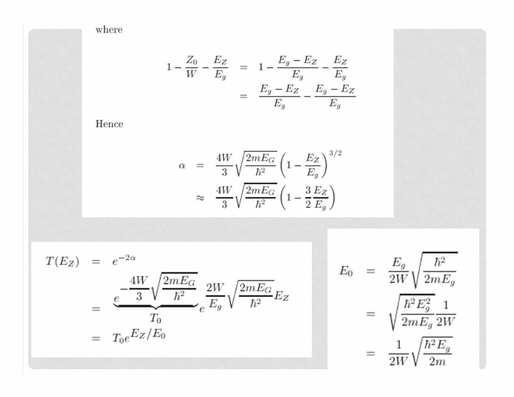
2T e

α−=

Transmission coefficient:

FOWLER-NORDHEIM TUNNELING

� The final expression for the Fowler-Nordheim tunneling coefficient is:

� Important notes:

� The above expression explains tunneling process only qualitatively because the additional attraction of the electron back to the plate is not included

� Due to surface imperfections, the surface field changes and can make large difference in the results

Φ−∝

�eE

mT B

3

*24exp

2/3

Calculated and experimental tunnel current characteristics for ultra-thin oxide layers.

(M. Depas et al., Solid State Electronics, Vol. 38, No. 8, pp. 1465-1471, 1995)

TRANSFER MATRIX APPROACH

TUNNELING: TRANSFER MATRIX APPROACH

Within the Transfer Matrix approach one can assume to have either

• Piece-wise constant potential barrier• Piecewise-linear potential barrier

PIECE-WISE CONSTANT POTENTIAL APPROXIMATION

Piece-Wise Constant Potential Barrier (PCPBT

Tool) installed on the nanoHUB

The Approach at a Glance

The Approach, Continued

Slide property of Sozolenko.

PIECE-WISE LINEAR POTENTIAL APPROXIMATION

PIECE-WISE LINEAR APPROXIMATION

• This algorithm is implemented in ASU’s code for modeling Schottky junction transistors (SJT)

• It approximates real barrier with piece-wise linear segments for which the solution of the 1D Schrodinger equation leads to Airy functions and modified Airy functions

• Transfer matrix approach is used to calculate the energy-dependent transmission coefficient

• Based on the value of the energy of the particle E, T(E) is looked up and a random number is generated. If r<T(E) than the tunneling process is allowed, otherwise it is rejected.

The Approach at a Glance

E

ai-1 ai

ai+1

Vi

Vi+1

Vi-1 V(x)

• 1D Schrödinger

equation:

• Solution for piecewise

linear potential:

• The total transmission

matrix:

• T(E):

ψψ ExVdx

d

m=+

Ψ− )(

2 2

22�

)()( )2()1( ξξψ iiiii BCAC +=

1 2 1........T FI N BIM M M M M M−=

12

011

1+= N

T

kT

Km

' '1 1

0 0

' '1 1

0 0

' '1 1

' '1 1

1 1[ (0) (0)] [ (0) (0)]

2 2

1 1[ (0) (0)] [ (0) (0)]

2 2

( ) ( ) ( ) ( )

( ) ( ) ( ) ( )

i i i i

FI

i i i i

N i N N i N N i N N i NBI

n N i N N i N N i N N i N

r rA A B B

ik ikM

r rA A B B

ik ik

r B ik B r B ik BM

r r A ik A r A ik A

+ +

+ +

+ +

=

− +

ξ + ξ ξ − ξπ =− ξ + ξ − ξ − ξ

'

' ''1 1

( ) ( )( ) ( )

( ) ( )( ) ( )

i i i ii i i i ii

i i i i i i ii i i i i

A BrB BM

r r A r BrA A + +

ξ ξ ξ − ξπ =

ξ ξ − ξ ξ

Simulation Results for Gate Leakage in SJT

10-7

10-6

10-5

10-4

10-3

0.1 0.2 0.3 0.4 0.5 0.6 0.7

Drain current Gate CurrentTunneling Current

Cur

rent

[A/u

m]

Gate Voltage [V]

T. Khan, D. Vasileska and T. J. Thornton, “Quantum-mechanical tunneling phenomena in metal-semiconductor junctions”, NPMS 6-

SIMD 4, November 30-December 5, 2003, Wailea Marriot Resort, Maui, Hawaii.

TSU-ESAKI FORMULA FOR THE CURRENT CALCULATION

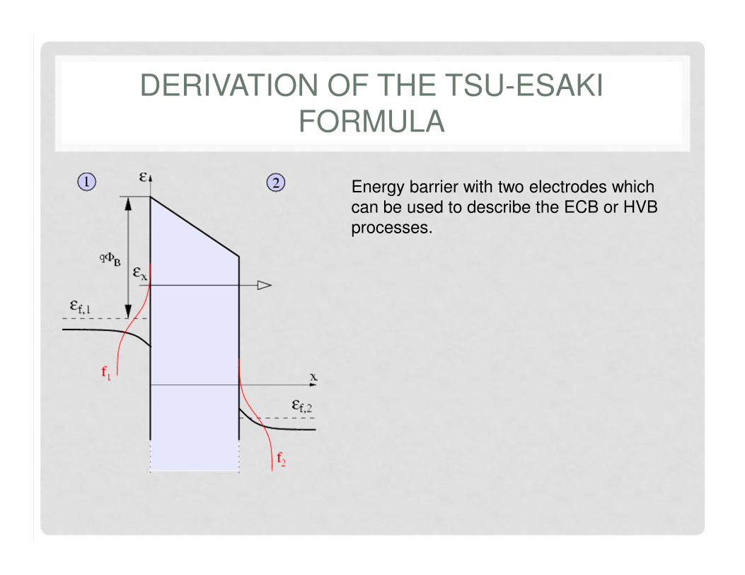
DERIVATION OF THE TSU-ESAKI FORMULA

Energy barrier with two electrodes which can be used to describe the ECB or HVB processes.

ASSUMPTIONS

• Effective mass approximation. The different masses corresponding to the band structure of the considered material are lumped into a single value for the effective mass. This is denoted by meff in the electrodes and mdiel in the dielectric layer.

• Parabolic bands. The dispersion relation in semiconductors is approximated by

• Conservation of parallel momentum. Only transitions in the kx direction are considered, the parallel wavevector k|| = kyey + kzez is not altered by the tunneling process.

( )2 2 2

2 2 2

2 2x y z

eff eff

kE k k k

m m= = + +� �

CURRENT CALCULATION

• The net tunneling current from Electrode 1 to Electrode 2 can be written as the net difference between current flowing from Side 1 to Side 2 and vice versa:

• The current density through the two interfaces depends on the perpendicular component of the wavevector kx, the transmission coefficient Tc, the perpendicular velocity vx, the density of states gc

and the distribution function at both sides of the barrier:

1 2 2 1J J J→ →= −

( )

( )1 2 1 1 2

2 1 2 2 1

( ) ( )[1 ( )]

( ) ( )[1 ( )]

c x x x x

c x x x x

dJ qT k v g k f E f E dk

dJ qT k v g k f E f E dk

→

→

= −

= −

CURRENT CALCULATION, CONT’D

• In this expression it is assumed that the transmission coefficient only depends upon the momentum perpendicular to the interface. The density of states g(kx) is:

• Where g(kx,ky,kz) denotes the three-dimensional density of states in momentum space. Considering the quantized wavevectorcomponents within a cube of side L yields for the density of states within the cube:

0 0

( ) ( , , )x x y z y zg k g k k k dk dk

∞ ∞

= ∫ ∫

3 3

2 1 1 2( , , ) ,

4x y z i

x y z

g k k k kL k k k L

π

π= = ∆ =

∆ ∆ ∆

CURRENT CALCULATION, CONT’D

• For the parabolic dispersion relation, the velocity and energy components in the tunneling direction obey:

• Hence, the expressions for the current density become:

1 1, and x

x x x x

x eff

kEv v dk dE

k m

∂= = =

∂

�

� �

( )

( )

1 2 1 23

0 0

2 1 2 13

0 0

( )[1 ( )]4

( )[1 ( )]4

c x x y z

c x x y z

qdJ T E dE f E f E dk dk

qdJ T k dE f E f E dk dk

π

π

∞ ∞

→

∞ ∞

→

= −

= −

∫ ∫

∫ ∫

�

�

CURRENT CALCULATION, CONT’D

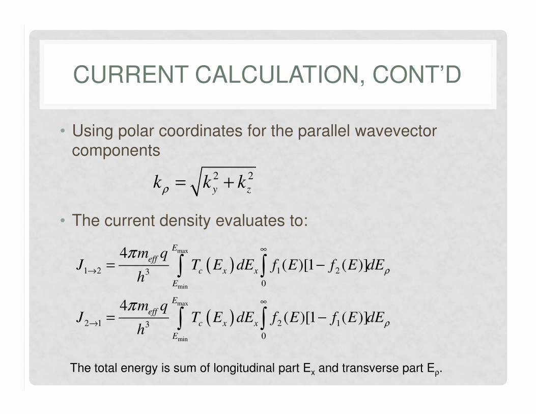
• Using polar coordinates for the parallel wavevectorcomponents

• The current density evaluates to:

2 2

y zk k kρ = +

( )

( )

max

min

max

min

1 2 1 23

0

2 1 2 13

0

4( )[1 ( )]

4( )[1 ( )]

E

eff

c x x

E

E

eff

c x x

E

m qJ T E dE f E f E dE

h

m qJ T E dE f E f E dE

h

ρ

ρ

π

π

∞

→

∞

→

= −

= −

∫ ∫

∫ ∫

The total energy is sum of longitudinal part Ex and transverse part Eρ.

CURRENT CALCULATION, CONT’D

• Evaluating the difference, the net current through the interface equals:

• This expression is usually written as an integral over the product of two independent parts which only depend upon the energy perpendicular to the interface: The transmission coefficient Tc(Ex) and the supply function N(Ex)

[ ]max

min

1 2 2 1 1 23

0

4( ) ( ) ( )

E

eff

c x x

E

m qJ J J T E dE f E f E dE

hρ

π ∞

→ →= − = −∫ ∫

max

min

3

4( ) ( )

E

eff

c x x x

E

m qJ T E N E dE

h

π= ∫

TSU-ESAKI FORMULA

• The expression in the previous slide is known as the Tsu-Esaki formula.

• The supply function describes the difference in the supply of carriers at the interfaces of the dielectric layer. Following the definition of the current, the supply function is given by:

• The occupancy functions f1 and f2 are defined near the interfaces. Since the exact shape of these distributions is usually not known, approximate shapes are commonly used. Furthermore, it is assumed that the distributions are isotropic.

[ ]1 2

0

( ) ( ) ( )x

N E f E f E dEρ

∞

= −∫

SUPPLY FUNCTION

• In equilibrium, the energy distribution function of electrons and holes is given by the FERMI-DIRAC statistics

• Which can be derived from statistical mechanics. Separating the longitudinal and the transverse energies E=Ex+Eρ, and splitting the integral N(Ex)=ξ1(Ex)-ξ2(Ex),

the values of ξ1 and ξ2 become:

1( )

1 expf

B

f EE E

k T

=−

+

0 0

1( ) , i=1,2

1 exp

i i

x fi

B

f E dE dEE E E

k T

ρ ρρ

ξ∞ ∞

= =+ −

+

∫ ∫

SUPPLY FUNCTION

• The last expression can be integrated analytically using:

• Then the total supply function is:

1ln

1 exp( ) 1 exp( )

dxC

x x

= +

+ + − ∫

1

2

1 exp

( ) ln

1 exp

f x

B

x B

f x

B

E E

k TN E k T

E E

k T

− +

= −

+