two dimensional numerical simulation of …rdio.rdc.uottawa.ca/papers/1- two dimensional...

- 258 - International Journal of Sediment Research, Vol. 19, No. 4, 2004, pp. 258-277

TWO DIMENSIONAL NUMERICAL SIMULATION OF FLOW AND GEO-MORPHOLOGICAL PROCESSES NEAR HEADLANDS BY

USING UNSTRUCTURED GRID

A. MOHAMMADIAN1, M. TAJRISHI2 and F. LOTFI AZAD3

ABSTRACT A two-dimensional mathematical model for simulating flow and sediment transport is presented.

The model simulates flow and geo-morphological processes using a high order accurate, oscillation free scheme. The depth averaged Reynolds (shallow water) equations are used for flow simulation. Both equilibrium and non-equilibrium methods (by solving convection-diffusion equation) are used for sediment transport modeling while sediment carrying capacity is computed using different methods. A finite volume, flux difference splitting scheme is employed to solve the governing equations, which is able to simulate sub, super and transcritical flows with shock waves. Moreover, the numerical method is able to simulate flow over the variable topographies and it has a low level of numerical diffusion in the case of circulating flows like headlands. The computational grid of this model is triangular unstructured with variable size, which is flexible for arbitrary geometries and grid refinement. Using the model for simulating flow and sediment transport in some test cases such as a partially closed channel and comparing the results showed that the results obtained by the developed model were in a reasonable agreement with measurements and the other models cited. Key Words: Flow, Geo-morphological processes, Shallow water, Unstructured grid

1 INTRODUCTION

In recent years, due to the increase in population and industrial developments, mankind has faced many problems associated with rivers, coastal waters and reservoirs. Some of these problems are flood control, water supply, power generation, and irrigation. In addition, making new hydraulic structures changes natural conditions. Prediction of these changes is necessary for designing such constructions. For solution of these problems usually an assessment of flow pattern, sediment transport, morphological processes, and water quality is required. These problems can be solved by experimental and mathematical modeling. In recent years, due to the improvement of computational facilities, mathematical modeling has become applicable to most of these problems.

A large variety of methods are presented in the literature including probabilistic and deterministic approaches (Van Rijn, 1993). In the Deterministic approaches, two families of sediment modeling have been used, which are Eulerian and Lagrangian methods. In the Eulerian schemes the sediment is modeled by empolying a convection-diffusion equation for sediment concentration with a source term, while in the Lagrangian methods, the sediment and fluid are considered as two different phases, and the sediment particles are tracked in the flow filed (Shams et. al., 2002 and Wu and Wang, 2000a). Here the Eulerian method is followed. Based on the situation, one, two or three dimensional models are employed to simulate the sediment transport process. Although many one dimensional model are presented in the

1 Ph. D. Candidate, Dept. of Civil Engineering, Sharif University of Technology, Tehran, Iran,

E-mail: [email protected] 2 Assistant Professor, Dept. of Civil Engineering, Sharif University of Technology, Tehran,

Iran, E-mail: [email protected]

3 Research Associate, Dept. of Comput. Hydr., Water Research Center, Tehran, Iran, E-mail: [email protected]

Note: The original manuscript of this paper was received in May 2003. The revised version was received in April 2004. Discussion open until Dec. 2005.

International Journal of Sediment Research, Vol. 19, No. 4, 2004, pp. 258-277 - 259 -

literature (Zhou et. al., 1998, Fraccarollo et. al., 2003, Guo et. al., 2000, Yeh et. al.,1995) they are restricted to few cases due to their high level of simplifications. On the other hand three dimensional models (Wu et. al., 2000b, Gerges et. al., 1997, Wang and Zhou, 1996, Kolahdoozan and Falconer, 2003), despite of their high level of accuracy, are still too expensive for engineering applications.

Consequently, the depth averaged two dimensional models are widely used due to their efficiency and accuracy and many two dimensional models have been presented in the literature. Wang (1987) developed a two dimensional model using the space-staggered approximation on regular cartesian grid (Falconer, 1980). Shimizu and Itakura (1989) developed a model to calculate bed variations in channels under steady flow conditions. In their model, the governing equations of flow and sediment transport are solved in a cylindrical coordinate system, which is valid only for a specific geometry. Kassem and Chaudry (2002) developed a 2D depth averaged model using the curve-linear coordinate system with the equilibrium method. Equilibrium assumption restricts the model to few applications. Moreover their model is based on structured grids, which is not flexible for some real applications. Unstructured grids, which are used in this paper, are attractive because they can be used in irregular geometries and the elements may have arbitrary sizes in regions of interest. Soulis (2002) developed a two dimensional depth integrated model, with a fully coupled solution method. He used an accurate numerical scheme which is able to simulate sub and supercritical flows. However, this model is only based on equilibrium assumption and structured grid. Guo et. al. (2002) developed a non-equilibrium model, with capability of modeling nonuniform sediments, but their model is restricted to quasi-steady state conditions and structured grids.

Most current hydrodynamic models of rivers, reservoirs and tidal harbors are based on finite difference solution of depth averaged shallow water equations. With the finite volume methods we can employ an unstructured grid. Moreover, the finite volume methods can easily analyze sub, super and trans-critical flows. Extensive research has been performed in this area and many finite volume schemes are developed for the shallow water equations. For most of them, the flux vector is determined based on the wave propagation structure. However the finite volume methods have some problems in simulating bed variations.

Apart from the capability of simulating complicated flow regimes, the flow solver must have the following properties for the case of morphological processes

(i) The model should be able to consider variable topographies. In practical applications, morphological processes are usually very slow. Therefore, flow solvers which cannot accurately simulate the effect of bed topography, lead to erroneous results in long term simulations.

(ii) For special case of recirculating flows like Headlands, the model should have a low level of numerical diffusion, otherwise the numerical diffusion will lead to a short length of recirculating zone which will cause high errors in simulating morphological processes.

Most finite volume methods face problems in the case of variable topographies. During the past decade, some treatments have been proposed to overcome this difficulty such as: upwind discretization of the source terms (Bermudez and Vazquez-Cendon (1994), Vazquez-Cendon (1999) and Hubbard and Navarro (2001)), introducing a Riemann problem inside a cell, (LeVeque, 1999), Central-Upwind scheme (Kurganove and Levy, 2002), analytical solution for variable topography, (Alcrudo and Benkhaldon, 2001), WENO schemes (Vukovic and Sopta, 2002), the interface method (Jin, 2002), gas kinetic schemes (Xu, 2002) and ENO schemes, (Nujic, 1995). However, most of these schemes have problems in the case of circulating flows and/or they are not directly extendable for unstructured grids.

Zhou et. al. (2001) introduced the surface gradient method and showed that interpolating the depth without considering the bed variations may lead to erroneous results. They used the interpolated water surface elevation at the interface for calculating the source terms and showed that this approach with the HLL flux function (Harten and Hyman, 1983) leads to accurate results. Their scheme performs well for variable topographies, however, it is not extendable for unstructured grids and moreover, the HLL flux leads to a high level of numerical diffusion in recirculating flows.

Mohammadian et. al. (2003) proposed a modification to the Roe’s scheme. In this method the gravity terms are extracted from the flux terms and they are combined with the source terms. The surface gradient method (Zhou et. al., 2001) is then used as the interpolation scheme. The resulting scheme was found to have a proper performance not only in the case of flows with variable topography, but also for circulating


flows without any extra upwinding of source terms. Moreover it is not restricted to structured grids, and it can be employed easily with unstructured grids.

This research aimed at developing a model based on unstructured triangular grids for simulating flow and sediment transport. To this end, we combine the proposed flow solver (Mohammadian et. al., 2003) with an accurate sediment transport module to construct an efficient numerical model for various cases. The unstructured grid and capability of simulating complicated flow cases, lead to an effective and robust model for engineering applications.

This paper is organized as follows: In section 2 the governing equations of shallow flows are presented and the finite volume method for shallow water equations is explained. In section 3 the governing equation of sediment transport is reviewed and the numerical solution of the sediment transport equations is explained. In section 4, the performance of the proposed numerical method is tested for different cases and those are compared with exact solutions and available data. Some concluding remarks complete the study. 2 FLOW SIMULATION In this section the shallow water (SW) equations are introduced and the numerical solution procedure using the finite volume method on unstructured grid is reviewed. 2.1 Governing Equations The 2-D SW equations in a conservative form may be written as

dFSFt

U rrrr

∇+=∇+∂∂ , (2.1)

with ( )vhuhhU ,,=r

, ),( GEFrrr

= and

+=

+=

22

22

5.0,5.0

ghhvuvhvh

Guvh

ghhuuh

Err

, (2.2)

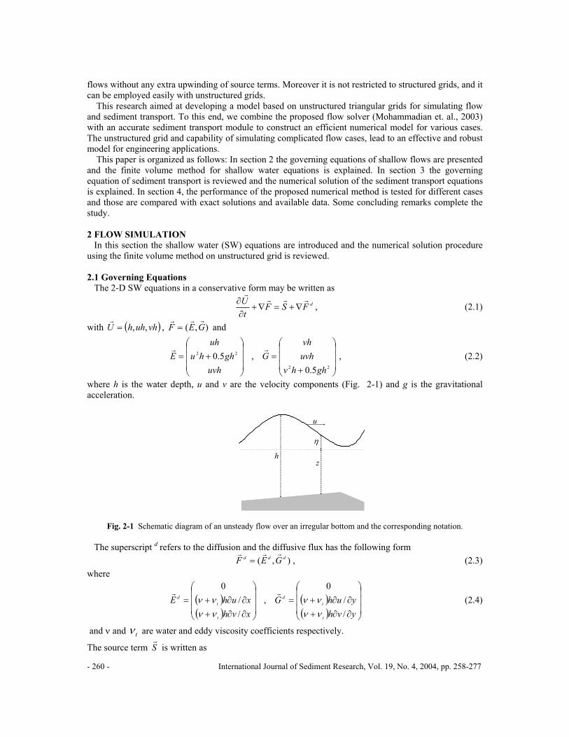
where h is the water depth, u and v are the velocity components (Fig. 2-1) and g is the gravitational acceleration.

Fig. 2-1 Schematic diagram of an unsteady flow over an irregular bottom and the corresponding notation.

The superscript d refers to the diffusion and the diffusive flux has the following form

),( ddd GEFrrr

= , (2.3) where

( )( )

( )( )

∂∂+∂∂+=

∂∂+∂∂+=

yvhyuhG

xvhxuhE

t

td

t

td

//

0 ,

//

0

νννν

νννν

rr (2.4)

and ν and tν are water and eddy viscosity coefficients respectively.

The source term Sr

is written as

η

hz

u


∂∂++

∂∂++=

yzghvucxzghvuucS

f

f

//

0

22

22

ν

r, (2.5)

where z is the distance between the bed surface and the reference level (Fig. 2-1) and fc is the friction coefficient. The SW equations may also be written in a non-conservative form

dFSyUB

xUA

tU rr

rrr

∇+=∂∂

+∂∂

+∂∂ , (2.6)

where A and B are the Jacobian matrices

+−−=

∂∂

=

−+−=

∂∂

=vcv

uvuvUGB

uvuvucu

UEA

20

100,02

010

22

22 r

r

r

r

, (2.7)

and ghc = is the wave velocity.

The eigenvalues ia and ib , (i=1,2,3) corresponding to the matrices A and B respectively are cuauacua −==+= 321 , , and cvbvbcvb −==+= 321 , , , respectively.

For all reported applications here (except mentioned), the eddy viscosity is computed form 22

2vuh

Cg

t +=ν ,

where nhC /6/1= is the Chezzy coefficient. 2.2 Numerical Solution of the Shallow Water Equations

A finite volume method using triangular grid is used in this paper. The variables are located herein at the geometric centers of the cells, and each triangle represents a control volume. Let A be the area of a triangle with boundary s. The SW equations are integrated over every control volume

.0=

∇−−∇+

∂∂

∫ ∫td dtdFSF

tU

AA

vvvr

(2.8)

The time integration is performed by using the first order forward (explicit) Euler time-stepping scheme, which leads to

( ) .01

=

∇−−∇+

∆−

∫+

AAdFSF

tUU nd

nn vvvrr

(2.9)

The application of Gauss theorem to the diffusive and convective flux integrals gives ( ) ( )dsnFnFdFF dd ∫∫ ⋅−⋅=∇−∇

sAA

vvvvvv, (2.10)

and the boundary integral is approximated by a summation over the triangle edges

( ) ( )∫ ∑=

⋅−⋅=−⋅−⋅s

kkk

dkkk

d dsnFnFdsnFnF3

1

rrrrrrrr. (2.11)

The diffusive fluxes may be approximated by a centered scheme ( )d

Ld

Rd FFF

rrr+= 5.0 (2.12)

and the convective flux Fr

is calculated here by a Godunov-type scheme ( )*5.0 FFFF LR

rrrr∆−+= , (2.13)

where ( ) ( )RRLL UFFUFFrrrrrr

== and are the left and right flux vectors. The subscripts .R and L. represent

the evaluation of the right and left sides of the interface, respectively, and *Fr

∆ is the flux difference based on the Roe’s linearization

∑=

=∆3

1

* ~ ~ ~

k

kkk eaFrr

α , (2.14)


where ka~ and ke~ r

are respectively the eigenvalues and eigenvectors of A~ , which is the Roe’s average Jacobian matrix, and satisfies UAF

rr∆=∆

~ with

( ) ( )( )

+−+−+−−=

∂∂

=

yxxyx

yyyx

yx

nvnunvnvcnvununvnunvunuc

nn

unFA

~2~~ ~~~~~~~2~~ ~~

0.~

22

22r

rr

, (2.15)

where

2)(~ , ~ , ~LR

LR

LLRR

LR

LLRR hhgchh

hvhvv

hh

huhuu +=

+

+=

+

+= . (2.16)

and the eigenvalues of A~ are simply cnvnua yx~~~~1 ++= , yx nvnua ~~~ 2 += , cnvnua yx

~~~~3 −+= , (2.17) with the corresponding eigenvectors

−−=

−=

++=

y

x

x

y

y

x

ncvncue

ncnce

ncvncue

~~~~

1~

, ~~0

~ ,

~~~~

1~ 321 rrr

, (2.18)

respectively. The coefficients kα~ are computed as (Alcrudo and Navarro, 1993)

( ) ( )[ ]hnvnunhvnhuc

hyxyx ∆+−∆+∆±

∆= )~~(~2

12

~ 3,1α , (2.19)

( )[ ] ( )[ ]( )yx nhuhunhvhvc

~ - ~ ~1~ 2 ∆−∆∆−∆=α . (2.20)

In this method, if the term of bed slope is considered in source terms, then on cell centered unstructured grid with variable topography, difference in discretization method for the terms leads to incompatibility and numerical error. One way is to discretize the bed slope term in an upwind manner (similar to flux terms), which is too expensive for practical applications. 2.3 Treatment of Variable Topographies

As mentioned in the previous sections, the bed slope (BS) term xzgh ∂∂ / is included in the source term, and it is usually discretized using a centered scheme. This leads to an imbalance between the depth gradient (DG) term xhg ∂∂ /5.0 2 and the BS term and hence to an artificial source term in the numerical solution. In order to overcome this problem, Mohammadian et. al. (2003) followed Nujic’s method (1995) where 25.0 gh term is extracted from flux functions EG

rv, and this leads to

=

=

hvuvhvh

Guvh

huuh

E2

2 ,rr

. (2.21)

The 0.5gh2 term is then combined with )( , )( yzghxzgh ∂∂∂∂ . The resulting terms )( xHgh ∂∂ ,

)( yHgh ∂∂ are considered as source terms, where H is the water surface elevation (height of water surface above a nominal zero level). Nujic used Shu and Osher (1988) scheme for computing flux vector, which produces a high level of numerical diffusion in the case of recirculating flows. In order to reduce the numerical diffusion of Nujic method, Mohammadian et. al. (2003) proposed a compatible version of Roe’s approximate solver in which, the surface gradient method (Zhou et. al. 2001) was employed as the interpolation method (see section 3.4). By applying this approximation to the Roe’s method, in the case of stagnant water, the U

r∆ is


−−−

=∆

LLRR

LLRR

LR

hvhvhuhu

HHUr

and the coefficients of decomposition of A~ are computed by

( ) ( )[ ]Hnvnunhvnhuc

Hyxyx ∆+−∆+∆±

∆= )~~(~2

12

~ 3,1α , (2.22)

( )[ ] ( )[ ]{ }xx nHuhunHvhvc

~ - ~ ~1~ 2 ∆−∆∆−∆=α . (2.23)

Mohammadian et. al. (2003) showed that this approach leads to accurate results in the case of variable topographies and also for recirculating flows. Further theoretical and numerical discussions about the flow solver and its performance in challenging test cases have been presented in Mohammadian et. al. (2004). 2.4 Flux Correction for Transcritical Flows

Roe’s method violates the entropy condition in the cases of sonic rarefactions (transcritical flows), and produces a shock inside a sonic rarefaction. Here we use the correction proposed by van Leer et. al. 1989, and used by Bradford and Sanders (2002). In this method the eigenvalues ia~ ,i=1,3 in (2.19) and (2.20) are modified when

2~

2aaa ∆

<<∆

− (2.24)

the corrected eigenvalues are

4

~ 2* a

aaa ∆

+∆

= (2.25)

( )LR aaa −=∆ 4 (2.26) 3 SEDIMENT TRANSPORT

Sediment transport is currently modeled in the literature based on two different approaches: equilibrium and non-equilibrium methods. Both of them are available in the present model as explained in this section. 3.1 The Equilibrium Method

In this method, it is assumed that the sediment concentration is in equilibrium conditions and hence, the sediment discharge through each cell face is computed using semi-empirical formulas. This leads to the following continuity equation for sediment transport

01

1 ,, =

∂

∂+

∂∂

−−

∂∂

yq

xq

ptz ytxt , (3.1)

where p is the porosity of sediments and xtq , and ytq , are sediment discharges in x and y direction, respectively. Different semi-empirical formulas are available for computing the sediment discharge in the present model including: the van Rijn (1984a,b) equation and its simplified version, the formula proposed by Soni et. al. (1980), and the Einstein’s method (1942). 3.2 The Non-Equilibrium Method

This method uses the convection-diffusion equation, which represents mass conservation and it is written as

( ) ( )cyx s

ych

yxch

xyvch

xuch

tch

+

∂∂

∂∂

+

∂∂

∂∂

=∂

∂+

∂∂

+∂∂ νν , (3.2)

where c is the sediment concentration; cs represents the source term, and xν and yν are horizontal sediment mixing coefficient in x and y directions respectively, and they are usually assumed to be equal to


the flow eddy viscosity ( tν ). The source term cs in (3.2) represents the net depth averaged erosion or deposition rate, which can be expressed in the form

( ) sc tcchs /ˆ −= , (3.3) where c =depth averaged equilibrium concentration

qq

c t=ˆ , (3.4)

where 22 vuhuhq +== and tq is the total equilibrium load . In (3.3), st is a time scale of deposition (or erosion) of the )ˆ( cc − concentration

)/( ss wt λ= , (3.5) where sw is the particle fall velocity and λ is the height of mass center in equilibrium concentration profile. As it is explained in the next section, λ can be written in term of h as hγλ = and hence the source term can be determined from the following formula

( ) γ/ˆ ccws sc −= . (3.6)

The bed change in this method is computed based on the source/sink term cs in (3.2) as

ps

tz c

−=

∂∂

1 (3.7)

3.2.1 The Coefficient of Sediment Source/Sink Term (γ)

In steady uniform flow, the time averaged downward transport of sediment by gravity is equal to the upward transport by the turbulent velocity fluctuations. In this case the sediment concentration profile may be expressed as

0=+dzdccw ss ε , (3.8)

where sε is the diffusion or mixing coefficient, and it can be approximated with a parabolic vertical profile as

−=

hz

hzhuzs 1)( *βκε , (3.9)

where β is the ratio of sediment and fluid mixing coefficient, *u is the overall bed-shear velocity, and κ =0.4 is the Von Karman constant (see appendix I). The sediment concentration profile in this case is

Z

a ahzzhacc

−−

=)()( , (3.10)

where

*u

wZ s

βκ= (3.11)

is the suspension number. The mass center of this profile can be approximated by

hdzzc

dzzzch

a

h

a γλ ==∫∫

)(

)(, (3.12)

where

∫

∫

−

−

=1

/

1

/

1

1

ha

Z

ha

Z

dtt

t

dtt

ttγ , (3.13)

with 5.00 ≤< γ . There is no analytical solution for integrals in (3.13). However, they can be calculated


numerically at the beginning of simulation with a typical value of ha / and the usual range of suspension number 20 ≤< Z . A typical plot of γ for 01.0/ =ha is presented in Fig. 2.

γ

Fig. 2 The profile of γ for ha / =0.01

In the numerical calculations, the profile of γ for a dominant value of ha / is calculated at the

beginning of simulation and it is saved in an array. Therefore, during the simulation, the local value of γ at each point of the domain can be easily interpolated from this array by using the corresponding local Z of that point. 3.3 Numerical Solution of Sediment Transport Equation

Numerical solution of (3.2) is similar to the shallow water equations. It is written in the following conservative form

cd sFF

tch

+∇=∇+∂∂ rr

, (3.14)

with convection and diffusion fluxes ) , ( vchuchF =

r, (3.15)

and

∂∂

∂∂

=ychv

xchF yx

d , νr

, (3.16)

respectively. Integrating (3.14) over an arbitrary triangular control volume and applying the Gauss divergence theorem, the following form is obtained

( ) ( ) ( ) ( ) ii AA ck

kkd

k

kkni

ni slnFlnF

tchch

+∆=∆+∆−

∑∑==

−− 3

1

3

1

11

..rrrr

, (3.17)

where nv is the normal vector on triangle edges. The convection flux on each edge of the triangle (see Fig. 3) is calculated as

( ) ( )[ ]LRRL ccqcqcqlnF −++=∆ 5.0.rr

, (3.18)


Fig. 3 A typical finite volume cell

where q is the total fluid flux

( ) ( )1212 xxvhyyuhq −−−= . (3.19) In (3.19), Lc and Rc are the values of c at left and right sides of edge, and they are calculated by the k scheme which is described in the next section. The diffusion flux is also calculated with a central scheme as

( ) ( ) ( )1212 22. xx

ych

ych

yyxch

xch

lnF RLRLd −

∂∂

+

∂∂

−−

∂∂

+

∂∂

=∆νννν

rv. (3.20)

3.4 Interpolation Scheme

The values of the variables at the left and right sides of the interface are needed to compute the numerical fluxes in (2.12) and (2.13). Various methods have been proposed for developing upwind higher order accurate models. Here, we use a MUSCL type approach, that has been proposed by van Leer (1982), based on an upwind monotonic approximation of the variables. Those are located in two adjacent triangles as shown in figure 4.

p bL

lL lRbR

Fig. 4 Two adjacent triangles with barycenters bL and bR, where lL and lR are the lengths

between the mid-side node of the common face and bL and bR, respectively. For a scalar variable c, the interface values Lc and Rc (on the left and right sides of a given face respectively) are

calculated by the κ scheme (Battina 1990). For example, Lc is calculated as

( ) ( )[ ]+− ∆++∆−+= kskssccLbL 11

4, (3.21)

( ) ( ) ( )LRL bb

RL

Lpb ccll

lcc −

+=∆−=∆ +−2, . (3.22)

where κ = -1 leads to a completely upwind scheme, κ = 0 to the Fromm scheme, κ = 1 to a central scheme and κ =1/3 to a third order scheme (in 1-D). We will use κ = 1/3 in the following. The slope limiter s, is chosen according to Battina (1990)

εε+∆+∆+∆∆

=+−

+−

22

2s , (3.23)

uv

1

1

yx

2

2

yx

3

3

yx


where ε is a very small number for avoiding division by zero in the regions of mild slope. We also follow the Zhou et. al. (2001) approach who interpolate the water surface elevation η at the cell faces instead of the water depth. Once Lη is calculated, the water depth can be obtained as

eLL zh +=η , (3.24) where ez is the distance between the bed surface and the reference level at triangle edge midpoints. The surface gradient method leads to 0=∆h at the cell faces in the case of stagnant water conditions and gives accurate results for variable topographies. An interpolation procedure is also used to calculate the depth integrated velocities uh and vh at cell faces, and this leads to

L

LL h

uhu )(= . (3.25)

3.5 Calculation of Derivatives The derivatives of a scalar variable c in unstructured grid may be calculated as (using the divergence theorem)

iii

ycycycd

xc

xc

AA

A A

3322111 ∆+∆+∆≈

∂∂

=

∂∂

∫ , (3.26)

iii

xcxcxcd

yc

yc

AA

A A

3322111 ∆+∆+∆−≈

∂∂

=

∂∂

∫ , (3.27)

1

1

yx

Lc1

Rc1

Lc3

Rc3

Rc2 Lc2

3

3

yx

2

2

yx

Fig. 5 Calculating the derivatives where (see Fig. 5)

231 yyy −=∆ , 231 xxx −=∆ , 2/)( 111RL ccc += , (3.28)

312 yyy −=∆ , 312 xxx −=∆ , 2/)( 222RL ccc += , (3.29)

123 yyy −=∆ , 123 xxx −=∆ , 2/)( 333RL ccc += . (3.30)

This approach may be used for calculating the viscous terms, i.e.

ii

i

ycycych

xch

A332211 ∆+∆+∆

≈

∂∂ νν . (3.31)

A similar approach is employed to calculate the viscous term of flow equations i.e. xuh ∂∂ /ν and xvh ∂∂ /ν .


4 NUMERICAL RESULTS AND COMPARISONS In order to study the performance of the numerical scheme, some test cases are presented herein. The first two cases show the performance of the model in simulating equilibrium conditions while the other tests evaluate the model in non-equilibrium conditions. In the first three tests, one dimensional cases are simulated, while the forth test is performed to evaluate the result of the model in simulating morphological changes in a partially closed channel where a circulating flow occurs. All simulations were performed by selecting CFL numbers greater than 0.6 for flow and sediment modules. As shown in the following, no oscillation is observed in the results due to the variable topography, which shows that the source terms and flux gradients are accurately balanced contrary to most existing flux splitting schemes. 4.1 Aggradation due to Sediment Overloading Soni et. al. (1980) conducted some experiments in a laboratory channel 0.2 m wide and 30 m long to study the aggradation process. A unit discharge q = 0.02 m2/s and a uniform flow depth of 0.05 m were considered in the channel. The sand forming the bed and the injected material had a mean diameter of 0.32 mm. From the uniform flow experiments, the following sediment transport formula was proposed by Soni et. al. (1980)

5)(0.00145hqqt = (4.1)

The manning’s roughness coefficient n was approximately equal to 0.022, the porosity of the sediment bed layer was equal to 0.4, and the initial bed slope was 0.00356. The equilibrium between the water flow and the sediment flow was disturbed by increasing the sediment inflow at the upstream end from the equilibrium value of qt to 5qt. This resulted in the aggradation of the stream bed. The numerical modeling was performed using an unstructured grid shown in fig 6-1, by employing the equilibrium method. Fig. 6-2 shows the comparison between the computed transient bed and water-surface profiles with the measured values at t = 40 min. As can be seen, the mathematical model can reasonably simulate the aggradation of the channel bed as well as the transient water-surface.

Fig. 6.1 A part of the numerical grid used for the test 4-1

Fig. 6.2 Computed and measured water surface and bed level


4.2 Knickpoint Migration Knickpoints are defined as the points of abrupt change in the longitudinal bottom profile of a channel.

Brush and Wolman (1960) explained the migration of knickpoints as a result of erosion potential hSf becoming maximum at the point where slope changes. The flow is subcritical on the upstream side of the knickpoint, and it is supercritical on the downstream side. The model presented in the previous sections was used to predict the knickpoint migration and the accompanying bed-level changes in experiment conducted by Brush and Wolnian (1960). The experiment was conducted in a 15.8-m-long and 1.2-m-wide flume. The median size of sediments was 0.67 mm. A fall of approximately 0.0305 m (Fig. 7-2 ) was provided at 10.8 m from the upstream end. The slope of the channel above and bellow this point was approximately equal to 0.00125. Water was then turned on (q0= 0.0028 m2/s, h0=0.0305 m), and the bed levels were recorded at successive times.

The unstructured grid used to simulate this case is shown in Fig 7.1. An equilibrium approach was found to be appropriate. Sediment discharge was estimated using bed load formula of Einstein (1942)

fhsds

b egdsq501)-( 391.0

350 1)-(15.2

−

= (4.2) Fig. 7.2 compares the computed and measured results at t = 2 hours 40 min. Results of Bhallamudi and

Chaudhry (1991) are also presented in Fig. 7.2, The computed bed profile satisfactorily matches the measured bed profile despite the inherent uncertainty in the sediment transport equation. As can be seen from Fig. 7.2, results of the current model are closer to the measurements than those predicted by Bhallamudi and Chaudhry (1991).

Fig. 7.1 Numerical grid used for the test 4-2

Fig. 7.2 Computed and measured bed level

4.3 Migration in Trench

In this case study, the results obtained from a series of experiments carried out at Delft Hydraulics by van Rijn (1980) were used. The experiments carried out in a 30 m long, 0.5 m wide, and 0.7 m deep flume with a trench of 1:10 side-slop. The characteristic diameters of the sediment material were 50D = 160 µm and 90D = 200 µm. The water depth and mean fluid velocity were 0.39 m and 0.51 m/s respectively. During the experiments, the equilibrium conditions were maintained in the upstream end. The sediment density was assumed to be 2650 3mkg and the porosity of the bed material was 0.4. The numerical grid employed for simulating this problem is presented in Fig. 8.1. The numerical results obtained by using the non-equilibrium method are presented in Fig. 8.2 and they are compared with measured data and results of the equilibrium method. As can be seen in Fig. 8.2, the non-equilibrium method can closely reproduce the experimental data, while the equilibrium method leads to large errors. The equilibrium concentration in (3.4) was computed by the simplified van Rijn method (Appendix I).


Fig. 8.1 A part of numerical grid used for the trench test

Fig. 8.2 Comparison between the result of the present model and measured data 4.4 Morphological Changes in a Partially Closed Channel

In order to verify the model and compare the results, a partially closed channel 3 km long and 1 km wide was considered under the steady state flow conditions. Although this was an academic case, a number of different models have been applied to this case. A 0.4 km long headland was located in the middle of the channel (Fig. 9.1). For this study, non-cohesive bed material with 50D = 0.2 mm and 90D = 0.3 mm was chosen. The bed roughness height was assumed to be 0.25 m and the horizontal mixing coefficient for flow and sediment was 0.5 sm 2 in each direction. The upstream hydrodynamic boundary condition was assumed to be 4000 discharge and downstream boundary was 6 m depth (Kolahdoozan 1999). The equilibrium concentration in (3.4) was computed by the van Rijn method (Appendix I).

Fig. 9.1 Schematic view of channel

Fig. (9.2) shows the used grid and streamlines in the developed model. Results of other models are also presented herein to compare with the present model. The three-dimensional model GEO- DIVAST (Kolahdoozan 1999) is a modified version of DIVAST (Falconer 1980) and uses a finite volume method. The model SUTRENCH is a finite element model, which was developed by Delft Hydraulics (Van Rijn 1987) and considers the vertical profiles of flow and sediment. Fig. s 9.3 and 9.4 show the depth averaged flow field obtained from the developed model and GEO-DIVAST model (Kolahdoozan, 1999), respectively. Based on comparison of results in the Figs. (9.3) and (9.4), the results obtained from developed model and GEO-DIVAST model were in good agreement.

y

3000 m

1000 m

400 m

Q


Streamline AStreamline B

Streamline C

Fig. 9.2 Streamline pattern obtained from developed model

Fig. 9.3 Flow velocity obtained from developed model

Fig. 9.4 Flow velocity obtained from GEO-DIVAST model

For more comparisons, the results of the depth-averaged velocities obtained from different models

along streamline B and C are shown in Figs. (9.5) and (9.6). In these Fig. s the results obtained from the developed model are compared with three different models. The model ESMOR was also developed in Delft Hydraulics by Wang (1989) and is a two dimensional depth averaged model. Based on a comparison of the results in Figs. (9.5) and (9.6), the results of the developed model are in a close agreement with other models.

Fig. 9.5 Depth averaged velocities along streamline B obtained from different models


Fig. 9.6 Depth averaged velocities along streamline C obtained from different models

Using the developed model the suspended sediment transport distribution was calculated and the

resulting flow pattern is shown in Fig. (9.7). For the GEO-DIVAST model, the corresponding pattern is shown in Fig. (9.8). The ratio of the maximum sediment concentration around the tip of the spur-dyke simulated by the present model and GEO-DIVAST is around 250/400= 62.5%. Hence, there is a maximum of 37.5% difference between the models, which is due to the difference between simulation approaches. However, this is not a uniform difference over the whole region of simulation. The difference rapidly reduces and in most parts the level of difference is acceptable and the models are in a close agreement. The resulting suspended sediment concentrations were compared between different models along the streamlines B and C and the results are shown in figs 9.9 and 9.10. A reasonable agreement is observed.

The rate of bed changes at the beginning of simulation predicted by using the developed model and the GEO-DIVAST model are shown in Fig. 9.11 and 9.12. A reasonable overall agreement is observed, which shows that in general the computed results back each other, but the present model is also capable of simulating complex geometries and different flow regimes, which is beyond the scope of classical models.

10

10

10

20

20

2050

50

50

100

100150

150

200

Fig. 9.7 Sediment concentration (mg/l) obtained from developed model

Fig. 9.8 Sediment concentration (mg/l) obtained from GEO-DIVAST model


Fig. 9.9 Suspended sediment fluxes along streamline B

Fig. 9.10 Suspended sediment fluxes along streamline B

-2 5-13 -7

-5-3-1

-1 1

1

3 3

3

Fig. 9.11 Rate of bed level change (mm/hr) obtained from developed model

Fig. 9.12 Rate of bed level change (mm/hr) obtained from GEO-DIVAST model


5 CONCLUSIONS A flux difference splitting numerical scheme was successfully employed for two-dimensional

simulation of flow and geo-morphological processes. The resulting model was found to be a convenient engineering tool for practical applications, due to the following features:

1. The model is based on unstructured triangular grids, which are attractive due to their capability of simulating complex boundaries and arbitrary local mesh refinement.

2. The numerical method is a Godunov-type mass conserving finite volume scheme on the basis of flux difference splitting. This scheme is able to simulate complex flows including sub, super and transcritical flows and shock waves with a high accuracy level.

3. Unlike most existing Godunov-type schemes, the present model employs a compatible treatment of source terms, and hence, it can simulate complex flows over variable topographies without leading to numerical oscillations.

4. Moreover, it produces a very low level of numerical diffusion in the case of circulating flows, which is crucial for an accurate simulation of bed evolutions around headlands.

5. Both equilibrium and non-equilibrium methods are available for sediment transport modeling. A number of tests were performed to evaluate the performance of the developed model in different test

cases including equilibrium and non-equilibrium conditions. The results of velocity, sediment concentration, and bed level change were compared with measured data and three other models in the literature. The results were in reasonable agreement and no oscillation was observed in the results due to the variable topography, which shows that the source terms and flux gradients are accurately balanced in the flow solver. ACKNOWLEDGEMENTS

This work was funded by Water Research Center of Iran, HEMAT project. REFERENCES Alcrudo, F. and BenKhaldoun, F. 2001, Exact Soloutions to the Riemann Problem of the Shallow-water Equations

with a Bottom Step, Computers and fluids 30, pp. 643-671. Alcrudo, F. and Garcia-Navaro, P. 1993, A high resolution Godonov-type scheme in finite volumes for the 2D

shallow-water equations. Int. J. Numer. Methods in Fluids, 16, p.489. Bermúdez, A. and Vázquez Cendon, M. E. 1994, Upwind methods for hyperbolic conservation laws with source

terms. Comput. & Fluids 23, p. 1049. Bhallamudi, S. M. and Chaudhry, M. H. 1991, Numerical modeling of aggradation and degradation in alluvial

channels. J. Hydr Engrg. ASCE, Vol. 117, No. 9, pp. 1145-1164. Batina, J. 1990, Implicit flux-split euler schemes for unsteady aerodynamics analysis involving unstructured dynamic

meshes, AIAA, Vol. 29, No. 11, p. 1836. Bermudez, A. and Vazquez, M. E. 1994, Upwind methods for hyperbolic conservation laws with source terms.

Computers and Fluids, 23, p. 1049. Bradford, S. F. and Sandres, B. F. 2002, Finite-volume model for shallow-water flooding of arbitrary topography, J.

Hydraulic Eng. ASCE 128, p. 289. Einstein, H. A. 1942, Formulas for the Transportation of Bed-Load, Vol. 107, Paper No. 2140, Transactions of the

American Society of Engineers, pp. 561-573. Falconer, R. A. 1980, Numerical modeling of tidal circulation in harbors, J. Hydraulic Eng. ASCE, Vol. 106, No. 1,

pp. 31-48. Fraccarollo et. al., 2003, A Godunov method for the computation of erosional shallow water transients, International

Journal for Numerical Methods in Fluids, 41, pp. 951-976. Gerges, H. and McCorQudale, J. 1997, Modeling of flow in rectangular sedimentation tanks by an explicit third-order

upwinding technique. Int. J. Numer. Methods in Fluids, 24, pp. 537-561. Guo, Q. C. and Jin, Y. C. 2000, Modeling sediment transport using depth-averaged and moment equations, J. Hyd.

Eng. ASCE, Vol. 125, No. 12, p. 1262. Guo, Q. C. and Jin, Y. C. 2002, Modeling nonuniform suspended transport in alluvial rivers, J. Hyd. Eng. ASCE,

Vol. 128, No. 9, p. 839. Harten, A. and Hyman, P. 1983, Self adjusting grid methods for one-dimensional hyperbolic conservation laws, J. of

Comput. Phys., 50, pp. 235-269. Hubbard, M. E. and Garcia-Navarro, P. 2001, Balancing source terms and flux gradients in finite volume schemes,

Godunov Methods: Theory and Applications, Edited by E. F. Toro, Kluwer Academic Publishers, New York, pp. 447-483.


Jin, S. 2001, Steady-state capturing method for hyperbolic systems with geometrical source terms, Math. Model Num. Anal. 35, pp. 631-646.

Kassem and Chaudry 2002, Numerical modeling of bed evolution in channel bends, J. Hyd. Eng. ASCE, Vol. 128, No. 5, p. 712.

Kolahdoozan, M. and Falconer, R. 2003, Three dimensional modeling of flow and sediment in estuaries and marine flows. Int. J. Sediment Research.

Kolahdoozan, M., 1999, Numerical modeling of geo-morphological processes estuarine waters, University of Bradford, UK, Ph. D. Thesis.

Kurganov, A. A. and Levy, D. 2002, Central-upwind schemes for the saint-venant system mathematical modeling and Numerical Analysis, 36 , 397-425.

LeVeque, R. J. and Derek, S. Bale 1999, Wave propagation methods for conservation laws with source terms. Int. Series. Num. Math. (130), pp. 609-618.

LeVeque, R. J. and Derek, S. Bale 1999, Wave propagation methods for conservation laws with source terms, Int. Series. Num. Math. 130, pp. 609-618.

Mohammadian, A. and Tajrishi, M. 2003, Simulation of shallow recirculating flows with variable topography using upwind schemes on unstructured grids. XXX IAHR Congress , Thessaloniki, Greece.

Mohammadian, A., Roux, D. Y. Le, Tajrishia, M. and Mazaheri, K. 2004, A mass conservative scheme for simulating shallow flows over variable topographies using unstructured grids, Accepted for publication in Advances in Water Resources.

Nujic, M. 1995, Efficient implementation of non-oscillatory schemes of free surface flows J. Hyd. Res., Vol. 33, No.1, p. 101.

Shams, M., Ahmadi, G. and Smith, D. 2002, Computational modeling of flow and sediment transport and deposition in meandering rivers, Advances in Water Resources, 25, pp. 689-699.

Shimizu, Y. and Itakura, T. 1989, Calculation of bed variation in alluvial channels, J. Hydraulic Eng. ASCE, Vol. 115, No. 3, pp. 367-384.

Shu C.W. and Osher, S. 1988, Efficient implementation of non-oscillatory shock-capturing schemes. J. Copmut. Phys., Vol. 77, pp.439-471.

Soni,J. P., Garde, R. J. and Ranga Raju, K. G. 1980, Aggradation in streams due to overloading. J. Hydr. Engrg., ASCE. Vol. 106, No. 1, pp. 117-132.

Soulis, J. V. 2002, A fully coupled numerical technique for 2D bed morphology calculations, International Journal for Numerical Methods in Fluids, 38, pp. 71-98.

Van Leer, B. 1982, Flux vector splitting of the euler equations, Lecture Notes in Physics, Vol. 170, pp. 507-512. Van Leer, B., Lee, W. T. and Powell, K. G. 1989, Sonic point capturing, 9th CFD conference, American Institute of

Aeronaotics and Astronautics, Buffalo, N.Y. Van Rijn, L. C., 1993, Principles of sediment transport in rivers, estuaries and coastal seas, Aqua Publications, The

Netherlands. Van Rijn, L. C., 1984a, Sediment transport part I: Suspended load transport, Journal of Hydraulic Engineering

(ASCE), Vol. 110, No. 10. Van Rijn, L. C., 1984b, Sediment transport part II: Suspended load transport, Journal of Hydraulic Engineering

(ASCE), Vol. 110, No.11, pp. 1613-1641. Vazquez-Cendon, M.E. 1999, Improved treatment of source terms in ppwind schemes for the shallow-water

equations in channels with irregular geometry, J. Comput. Phys., Vol. 43, No. 2, pp. 357-372. Vukovic and Sopta, L. 2002, ENO and WENO schemes with the exact conservation property for one-dimensional

shallow-water equations, Journal of Computational Physics 179, pp. 593-621. Wang, Z.B., 1989, Mathematical modeling of morphological processes in estuaries, Dissertation, Detlft Univ, of

Techn., The Netherlands. Wang, S. S. Y. and Zhou, D. 1996, A 3D numerical model of sediment laden turbulent turbulent flows, Int. J.

Sediment Research, pp. 54-80. Wu W. and Wang S.S.Y. 2000a, Mathematical models for liquid-solid two phase flow, Int. J. Sediment Research,

Vol. 15, No. 3, p. 30. Wu, W., Rodi, W. and Wenka, T. 2000b, 3D Numerical modeling of flow and sediment transport in open channels, J.

Hydraulic Eng. ASCE, Vol. 126, No. 4, pp. 863-883. Xu, K. 2002, A well-balanced gas-kinetic scheme for the shallow-water equations with source terms. Yeh, K. C., Li, S. J. and Chen, W. L. 1995, Modeling Non-uniform sediment fluvial process by characteristics

method, J. Hyd. Eng. ASCE, Vol.121, No. 2, p. 159. Zhou, J. and Lin, B. 1998, One-dimensional mathematical model for suspended sediment by lateral integration, J.

Hyd. Eng. ASCE, Vol. 124, No. 7, p. 712. Zhou, J. G., Causon, D. M., Mingham, C. G. and Ingram, D. M. 2001, The surface gradient method for the treatment

of source terms in the shallow-water equations, Journal of Computational Physics 168, pp. 1-25.


THE VAN RIJN METHOD

The algorithm of calculating the total load transport with the Van Rijn’s method (1984a and b) may be summarized as follows

22 vuu += = water velocity (m/s) ρρ /ss = = relative density (-)

( ) 3/1250* /)1( ν−= sgdD = particle parameter (-)

1* 24.0 −= Dcrθ , for 4 1 * ≤< D = the Shields critical mobility parameter (-)

64.0* 14.0 −= Dcrθ , for 01 4 * ≤< D

1.0* 04.0 −= Dcrθ , for 02 01 * ≤< D

29.0* 013.0 Dcr =θ , for 015 02 * ≤< D

055.0=crθ , for * 150 D<

crscrb gd θρρτ 50, )( −= , = critical bed shear stress (N/m2) according to Shields

=′

90312log18d

hC . = grain related Chézy coefficient ( sm /0.5 )

2

′=′

Cugb ρτ , = effective bed shear stress (N/m2)

crb

crbbT,

,

τττ −′

= = bed shear stress parameter(-)

)//(*5.0 16505084 dddds +=σ = standard deviation of bed material (-)

( )( )[ ] 50251011.01 dTd ss −−+= σ = the representative particle size of

( 50dds = for 25≥T ) suspended sediment (m)

ν18)1( 2

ss

gdsw

−= , for md µ 100 1 ≤< ` = fall velocity of sediment particles (m/s)

−

−+= 1

)1(01.0110

5.0

2

3

νν s

ss

gdsd

w , for md µ 1000 100 ≤<

[ ] 5.0)1(1.1 ss gdsw −= , for md µ 1000<

=

skhC 12log18 = overall Chézy coefficient ( sm /0.5 )

uC

gu5.0

* = = overall bed-shear velocity (m/s)

ska = = reference level (m)

3.0*

5.150015.0

DT

ad

ca = = reference concentration (-)

65.00 =c = maximum concentration (-)

5.2=ψ4.0

0

8.0

*

cc

uw as = stratification correction(-)

2

*

21

+=

uwsβ (with 2max =β ) = ratio of sediment and fluid mixing

coefficient(-)


*uw

Z s

βκ= = suspension number (-)

ψ+=′ ZZ , = suspension number (-)

( ) ( )( ) ( )Zha

hahaF Z

Z

′−−−

= ′

′

2.11

2.1

= shape factor (-)

as hcuFq = , = volumetric suspended load (m2/s)

3 )1(053.0 1.23.0*

5.150

5.05.0 ≥−= − TforTDdgsqb = volumetric bed load (m2/s)

3 )1( 1.0 5.13.0*

5.150

5.05.0 ≥−= − forTTDdgsqb

Sbt qqq += = volumetric total load (m2/s) with h = water depth(m)

sk = overall roughness height (m)

50d = the median particle diameter of bed material(m)

16d , 84d , 90d = characteristic diameter of bed material(m) ρ = water density (kg/m3)

sρ = sediment density (kg/m3) ν = water kinematic viscosity coefficient (m2/s) κ = constant of Von Karman (=0.4) A simplified version of the van Rijn’s method is expressed as follows (van Rijn, 1993)

( )2.1

50

4.2

5.0

50)1(005.0

−

−=

hd

gdsuu

huq crb

( )

6.0

*

50

4.2

5.0

50

1)1(

012.0

−

−=

Dhd

gdsuu

huq crs

where )3/12log(19.0 90

1.050 dhducr = for 0005.00001.0 50 ≤≤ d

)3/12log(5.8 906.0

50 dhducr = for 002.00005.0 50 ≤≤ d

two dimensional numerical simulation of …rdio.rdc.uottawa.ca/papers/1- two dimensional...

Documents