Latin American Applied Research 38:213-225 (2008)

213

TWO-FLUID MATHEMATICAL MODEL FOR COMPRESSIBLE FLOW IN FRACTURED POROUS MEDIA

A. L. KHLAIFAT†

Department of Chemical Engineering, Faculty of Engineering, Mutah University, Mutah 61710, Jordan khlaifat@mutah.edu.jo

† Director of Prince Faisal Center for Dead Sea, Environmental and Energy Research

Abstract−− A three-dimensional isothermal tran-sient compressible two phase flow of liquid and gas in a low permeability fractured porous media model has been developed from the general mass and mo-mentum balances using volume averaging tech-niques. The emphasis of the paper is on the available analytical and semi-empirical correlations and clo-sure relations. The interfacial mass and momentum transfer terms in the averaged formulation are ex-plained. The assumptions used in the model’s formu-lation are that a condition of capillary equilibrium exists throughout the media, momentum transfer between mobile fluid phases is negligible in the po-rous media and exists in the fracture, and fluid phase change has been neglected. The pore size distribution of the studied porous media was represented by three mean pore diameters: liquid pore network, gas pore network, and fractures. An average pore di-ameter and length for each network were deter-mined using the gamma distribution function. The model was validated and solved for a hypothetical porous media and fractured domain.

Keywords−− Two-Fluid; Fractured; Porous Me-dia; Capillary Pressure; Transient; Compressible Flow, Isothermal, Mass, Momentum Transfer.

I. INTRODUCTION The increased sophistication of oil/gas recovery tech-nologies has brought with it increased operating and material costs and therefore a greater demand for sound process designs. Mathematical models of fluids flow in petroleum and gas reservoirs have become key tools by which reservoir engineers develop and implement these designs. Using mathematical models together with vari-ous characterizations of the rock-fluid system being modeled, the engineer can test various operating strate-gies, compare different recovery technologies, and for-mulate hypotheses in diagnosing the performance of ingoing projects.

It is impossible to specify the microstructure in a re-alistic porous medium completely. Porous media can be characterized without specifying the porous geometry in all its details. The well-known approach of doing so is by constructing a simplified geometric model, like bun-dle of capillary tubes, grain models, network models, and percolation model, for each specific porous medium of interest.

Most of the models describing the flow through frac-

tured porous media, such as (Thomas et al., 1983; Ev-ans, 1982; Guzman and Khaled., 1992; Fung, 1993; Warren and Root, 1963; Zekai, 1988; Nitao, 1990; Ar-bogast, 1993; Celis et al., 1992; Lee and Tan, 1987; Alder and Thovert, 1999; Panfilov and Panfilov, 2000) were based on Zheltov’s model (Zheltov et al., 1960), and used his concept of dual-porosity dual-permeability region. They differentiate between two flow regions, one representing the discrete matrix where the other represents the continuous fracture network. Based on that, they considered mainly two types of equations: the equations describing flow in fracture system and equa-tions describing flow in the matrix.

The main objective of the manuscript is the devel-opment of a mathematical model which predicts the flow phenomena in low permeability fractured porous media. It is rather impossible to apply conservation laws directly to each pore in porous medium and to find a possible numerical or analytical solution. Instead a semi-empirical approach has been used where some constitutive equations are needed, and a set of equations are developed based on flow through the entire medium.

It is known in reservoir engineering that the produc-tive strata (producing formation or beds) could be made up of rocks described by the following characteristics and properties; porosity, permeability, granulemetric composition, elasticity, resistance to rupture, compres-sion, deformation and saturation. Using these character-istics and properties, the conditions of oil and gas fields’ development can be determined.

Pore structure of reservoir rocks is very complex. In the case of fractured porous media, the porosity can be placed into two classes: 1- Primary porosity, which is highly interconnected

and can be correlated with permeability, this could be the porosity of the homogeneous rocks. This re-gion always has high resistance (low permeability) to flow.

2- Secondary porosity, formed by a fracture, usually this porosity is the product of geological move-ments, hydraulic fracturing and chemical processes. Although it does not contain a fraction of fluid re-serve as large as that of the first class, it greatly af-fects the flow. Moreover, it has low resistance to flow compared to the primary porosity region.

For the case of low permeability fractured porous media a network model is developed, the simultaneous existence of two phases of water and gas is considered.

A. L. KHLAIFAT

214

The wetting fluid occupies the smaller pores while the non-wetting fluid occupies the larger ones, and when these two fluids exist in the same pore diameters, they move in plug flow fashion. Simultaneous two-phase flow exists in the fractures and similar flow patterns as in the case of two-phase flow in a pipe with momentum transfer across phase boundaries are assumed. Further, there is continuous movement of the rigid porous media due to changes in stress distribution, particularly during production.

The pore size distribution in the medium is repre-sented by three mean pore diameters: gas pore network, liquid pore network, and fractures. This representation along with the movement of the rock matrix assumption result in a model with five different phases: 1) gas in the porous matrix (gas network), 2) liquid in the porous matrix (liquid network), 3) gas in the fracture, 4) liquid in the fracture, and 5) rock matrix. An average pore di-ameter and length for each network were calculated using the gamma distribution function.

II. GOVERNING EQUATIONS In the formulation of the mathematical model the fol-lowing assumptions are made: 1) The reservoir matrix is homogeneous and isotropic.

Furthermore, there is inaccessible pore volume 2) The reservoir rock and the working fluids are slightly

compressible 3) Because of the absence of both thermal action and

chemical reaction, the process is considered to be isothermal

4) We assume a constant mass generation πm of phase π, where π can be either solid (β) or fluid (α) phase

5) Gas and liquid are immiscible; furthermore we as-sume that there is no slip condition at the interface between the phases

The continuity equation for the Cartesian system of co-ordinate may be written, in tensor notation, as: ( ) ππ

iπ

iπ muρρ =∂+∂ (1)

where: πρ∂ is the rate of accumulation of mass per unit volume at specific point (say p); ( )πiπ

i uρ∂ is the net flow rate of mass out of p per unit volume; πm is mass generation of phase π; and the momentum equation as: ( ) ( ) π

iππ

iππ

ijjπijj

πi

πj

πj

πi

π umFργPuuρuρ ++∂+−∂=∂+∂ (2)

where ( )πiπuρ∂ is the rate of π momentum increase at the fixed point (say p), ( )πiπ

jπ

j uuρ∂ is the net rate of π momentum carried into p by the fluid or solid flow

πj

πuρ , πijj P∂ is the net π pressure force at p, π

ijj γ∂ is the

net π stress force, where πijγ is the viscous stress tensor

for phase π, πi

πFρ is π body force at p, where πi

πi gF = if

gravity is the only body force we consider and πi

π um is momentum generation at point p.

III. AVERAGING PROCEDURE The governing equations were averaged using the vol-ume averaging technique. This technique has been used widely for flow in porous media. It was demonstrated by William and O’Neill (1976), that averaging tech-nique can be applied to various transport processes in porous media. William and O’Neill (1976), William and Sampath (1982) and Slattery (1972), were among the first to use this technique to develop the governing equations for flow in porous media. Other researcher such as (Dullien, 1975; Le Gallo, 1990; Pakdel, 1994; Jacob and Yehuda, 1992, and Al-Khlaifat, 1998) has applied this technique to multiphase flow system.

Volume averaging technique results in achieving manuscript initial objective which is to associate with every point in a porous medium a local volume average of the differential equations of continuity (1) and mo-mentum (2). When we say every point, we include the solid phase as well as the fluid phase and the solid-fluid phase interface.

The phase average of the continuity (1) and the mo-mentum (2) equations can be written as: ( ) ππ

iπ

iπ muρρ =∂+∂ (3)

and

( ) ( )

πi

ππi

ππijj

πijj

πi

πj

πj

πi

π

umFργP

uuρuρ

++∂+∂−

=∂+∂. (4)

Applying the averaging rules (William and O’Neill, 1976; William and Sampath, 1982), to each term of Eq. (3) and (4). When assuming the no slip condition at the interface and a constant mass generation for α phase, the final volume averaged continuity equation will take the following form: ααα

iαα

i

ααα muρερε =⎟⎠⎞⎜

⎝⎛∂+⎟

⎠⎞⎜

⎝⎛∂ . (5)

After accounting for the no-slip condition at the inter-face, the final form of averaged momentum equation will be:

( )⎪⎭

⎪⎬⎫

−++

+⎩⎨⎧ ⎟

⎠⎞⎜

⎝⎛∂+⎟

⎠⎞⎜

⎝⎛∂−

=⎭⎬⎫

⎩⎨⎧ ⎟

⎠⎞⎜

⎝⎛∂+⎟

⎠⎞⎜

⎝⎛∂

∫αβ*A

αi

αij

αij

ααi

αα

i

αααααij

αjij

αααj

ααi

αj

ααj

ααi

αα

dAnPγV1umε

gPεγεδPε

uuρεuρε

(6)

IV. CONSTITUTIVE EQUATIONS In general a fluid flow problem is governed by several equations. First there are the basic equation of continu-ity, three momentum equations and an energy relation. Second, there are the constitutive equations, which are not basic, but they do apply to group of substances. Various transport coefficients are introduced in the con-stitutive relations. They are quasi-thermodynamic prop-erties that depend on the composition of the fluid and its thermodynamic state. Third, the thermodynamics of fluid must be specified, this may be done through the

Latin American Applied Research 38:213-225 (2008)

215

fundamental equation s(ρ,e) for the substance, or, more commonly, through two equation of state P(ρ,T) and e(ρ,T). All of these equations are required to give a well-posed problem for a general flow situation.

For the considered isothermal case, in order to use Eq. (5) and Eq. (6) we must insert expressions for the density, pressure, and stress of each phase. Also mass and momentum transfer between the phases should be defined and inserted.

A. Pore Geometry and Volume Fractions It has been believed that the smaller pores in the con-solidated material of tight sands cause the segregation of mobile fluids such that the wetting fluid occupies the smaller pores. The non-wetting fluid, and possibly an immobile wetting fluid layer lining the walls, would therefore occupy the large pores of this water wet mate-rial. This is a result of the large difference between the gas and liquid pressure caused by the small radius of curvature of the gas-liquid interface.

In addition to the assumption that the mobile fluids are separated on a pore level, it has been assumed that two networks for the fractured porous media (Fig. 1) exist.

Based on this network assumption, five different phases exist in the model as specified bellow: I. Solid phase:

1. gas in low permeability porous media (gp) 2. liquid in low permeability porous media (lp) 3. rock matrix (r)

II. Fracture 1. gas in the fracture (gf) 2. liquid in the fracture (lf), Governing equations for all these phases should be

developed from Eq. (5) and Eq. (6). The volume fraction for each phase can be defined as:

V

x)(t,αVαε = (7)

where x)(t,α

V is the volume of phase α, which is a func-tion of the position of the volume element (V) in the reservoir and also a function of time. Using equation (7), the volume fraction for all five phases is:

1lfε

rε

lpε

qpε =+++ (8)

as it can be seen from Eq. (8) gas and liquid phases exist simultaneously in both pore and fracture networks, then one can determine the gas and liquid volume fractions, respectively, as:

V

x)(t,gfVx)(t,gpVgfε

gpε

gε

+=++ (9)

and

V

x)(t,lfVx)(t,lpVlfε

lpε

lε

+=++ , (10)

then, Eq. (8) can be rewritten as:

1rε

lε

gε =++ , (11)

but from the definition of porosity φ, which is defined as:

Figure 1: Network Model of Fractured Porous Media

lε

gε +=φ , (12)

equation (11) becomes:

rε1 −=φ (13)

B. Pressures The pressure under reservoir conditions is very high and depends on the location of production formation. Ac-cording to Huinink and Michels (2002) and Holditch (1989), the pressure for some reservoirs can reach sev-eral thousand psi (106 and 108 Pa). This requires taking the compressibility of moving phases into account. The α phase pressure Pα in the volume element was defined by the intrinsic average phase pressure

ααP , in what

follows and for simplicity the following notation is used: ααα PP = . (14)

In order to reduce the number of independent vari-ables in the model, the equation of state to relate the density to the pressure for each phase is used. Gas Equation of State The equation of state for compressible gas is: TRZnVP gggg = , (15) substitute for Vg=mg/ρg and ng=mg/Mg into the above equation, then, in both fracture and pore networks the gas density is:

RTZPMρ g

ggg = , (16)

where Mg is the gas molecular weight, pg is the pressure of the gas, Zg is the compressibility factor of the gas, R is the universal gas constant, and T is the temperature.

A. L. KHLAIFAT

216

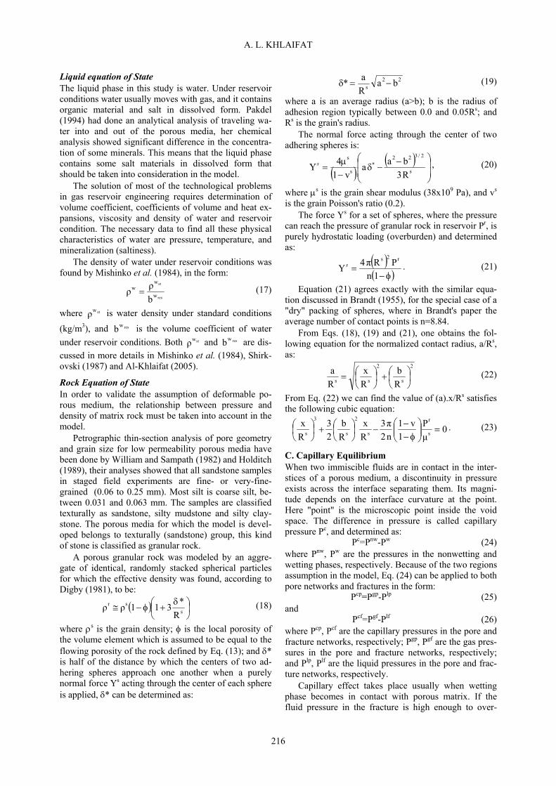
Liquid equation of State The liquid phase in this study is water. Under reservoir conditions water usually moves with gas, and it contains organic material and salt in dissolved form. Pakdel (1994) had done an analytical analysis of traveling wa-ter into and out of the porous media, her chemical analysis showed significant difference in the concentra-tion of some minerals. This means that the liquid phase contains some salt materials in dissolved form that should be taken into consideration in the model.

The solution of most of the technological problems in gas reservoir engineering requires determination of volume coefficient, coefficients of volume and heat ex-pansions, viscosity and density of water and reservoir condition. The necessary data to find all these physical characteristics of water are pressure, temperature, and mineralization (saltiness).

The density of water under reservoir conditions was found by Mishinko et al. (1984), in the form:

res

st

w

ww

bρρ = (17)

where stwρ is water density under standard conditions

(kg/m3), and reswb is the volume coefficient of water under reservoir conditions. Both stwρ and reswb are dis-cussed in more details in Mishinko et al. (1984), Shirk-ovski (1987) and Al-Khlaifat (2005).

Rock Equation of State In order to validate the assumption of deformable po-rous medium, the relationship between pressure and density of matrix rock must be taken into account in the model.

Petrographic thin-section analysis of pore geometry and grain size for low permeability porous media have been done by William and Sampath (1982) and Holditch (1989), their analyses showed that all sandstone samples in staged field experiments are fine- or very-fine-grained (0.06 to 0.25 mm). Most silt is coarse silt, be-tween 0.031 and 0.063 mm. The samples are classified texturally as sandstone, silty mudstone and silty clay-stone. The porous media for which the model is devel-oped belongs to texturally (sandstone) group, this kind of stone is classified as granular rock.

A porous granular rock was modeled by an aggre-gate of identical, randomly stacked spherical particles for which the effective density was found, according to Digby (1981), to be:

( ) ⎟⎠⎞

⎜⎝⎛ δ+φ−≅ s

sr

R*311ρρ (18)

where ρs is the grain density; φ is the local porosity of the volume element which is assumed to be equal to the flowing porosity of the rock defined by Eq. (13); and δ* is half of the distance by which the centers of two ad-hering spheres approach one another when a purely normal force Ys acting through the center of each sphere is applied, δ* can be determined as:

22s ba

Ra* −=δ (19)

where a is an average radius (a>b); b is the radius of adhesion region typically between 0.0 and 0.05Rs; and Rs is the grain's radius.

The normal force acting through the center of two adhering spheres is:

( )

( )⎟⎟

⎠

⎞

⎜⎜

⎝

⎛ −−δ

−μ

= ∗s

2/322

s

s

R3baa

v14Ys , (20)

where μs is the grain shear modulus (38x109 Pa), and vs is the grain Poisson's ratio (0.2).

The force Ys for a set of spheres, where the pressure can reach the pressure of granular rock in reservoir Pr, is purely hydrostatic loading (overburden) and determined as:

( )( )φ−=1n

PRπ4Yr2s

s . (21)

Equation (21) agrees exactly with the similar equa-tion discussed in Brandt (1955), for the special case of a "dry" packing of spheres, where in Brandt's paper the average number of contact points is n=8.84.

From Eqs. (18), (19) and (21), one obtains the fol-lowing equation for the normalized contact radius, a/Rs, as:

2

s

2

ss Rb

Rx

Ra

⎟⎠⎞

⎜⎝⎛+⎟

⎠⎞

⎜⎝⎛= (22)

From Eq. (22) we can find the value of (a).x/Rs satisfies the following cubic equation:

0μP

1v1

n2π3

Rx

Rb

23

Rx

s

r

s

2

s

3

s =⎟⎟⎠

⎞⎜⎜⎝

⎛φ−

−−⎟

⎠⎞

⎜⎝⎛+⎟

⎠⎞

⎜⎝⎛ . (23)

C. Capillary Equilibrium When two immiscible fluids are in contact in the inter-stices of a porous medium, a discontinuity in pressure exists across the interface separating them. Its magni-tude depends on the interface curvature at the point. Here "point" is the microscopic point inside the void space. The difference in pressure is called capillary pressure Pc, and determined as: Pc=Pnw-Pw (24) where Pnw, Pw are the pressures in the nonwetting and wetting phases, respectively. Because of the two regions assumption in the model, Eq. (24) can be applied to both pore networks and fractures in the form: Pcp=Pgp-Plp (25) and Pcf=Pgf-Plf (26) where Pcp, Pcf are the capillary pressures in the pore and fracture networks, respectively; Pgp, Pgf are the gas pres-sures in the pore and fracture networks, respectively; and Plp, Plf are the liquid pressures in the pore and frac-ture networks, respectively.

Capillary effect takes place usually when wetting phase becomes in contact with porous matrix. If the fluid pressure in the fracture is high enough to over-

Latin American Applied Research 38:213-225 (2008)

217

come capillary pressure in the matrix, the fluid penetra-tion into the pore networks occurs. Pressure required to overcome capillary forces at the entrance of the pore is called pore entry pressure. Capillary pressure value de-pends on the diameter of the pores in the pore networks and on the fracture openings in the fracture network.

Because of the two networks' assumption in the ma-trix, Eq. (24) can be written simultaneously for gas and liquid pore networks as the following: Pcgp=Pgp-Plf (27) and Pclp=Pgf-Plp (28) where Pcgp is the capillary pressure between the gas in the pore network and the liquid in the fracture; and Pclp is the capillary pressure between the liquid in the pore network and the gas in the fracture.

As long as Reynolds number in porous media is small, all of the above capillary equilibrium equations are valid under both static and dynamic conditions (Semrau, 1986). This pressure equilibrium across vari-ous interfaces of pores results in the equality between the sums of Eqs. (25-26) and Eqs. (27-28).

In the current model, under constant hydrostatic (overburden) pressure, the decrease of fluid pressure because of its production causes an increase which leads to closing the smaller diameter (water network) and decrease the number of interconnection between water and gas networks, this causes significant change in the rock matrix porosity, which modifies the mean pore sizes. Because of the deformable medium assumption, the average pore size for both liquid and gas networks will be found by using statistical approach (Section IV.G). The above effect does not take place in the frac-ture, because the later is composed of large pores that lead to minimal volume variations of the fracture net-work. Sources of useful information for the dynamic response of porosity to changes in rock pressure are limited and the information itself tends to be more qualitative than quantitative. Thus in the current model a constant fracture volume is acceptable in the consid-ered volume element, therefore εgf +εlf =const.

D. Gas and Liquid Mass Transfer The characteristic feature of an unsteady-state motion of a fluid in fractured rocks is the fluid transfer between the rock matrix and the fractures. Therefore, in investi-gating the flow of fluids in fractured porous medium it is necessary to take into consideration the outflow of fluids from the matrix blocks into the fractures.

The process of fluid transfer from the pores takes place essentially under a sufficiently smooth change of pressure, and, therefore, it can be assumed that this pressure is quasi-stationary, i.e. it is, explicitly, inde-pendent of time. It is obvious in such a case that during homogeneous fluid flow in the fractures, the volume of the fluid Vf, which flows from the matrix blocks into the fractures per unit of time and unit of volume of the rock, depends on the following (Zheltov, 1960),: (a) viscosity of the fluid μf; (b) pressure difference between the pores

and the fractures Pfp, Pff; and (c) certain characteristic of the rock, which can only be geometrical one, i.e. they might be the dimensions of length, area, volume, etc. The fluid volume was found to be: )P-(P

μηV fffp

ff = (29)

where η is some new dimensionless characteristics of the fractured rock; and Pfp, Pff are the fluid pressures in the pore and fracture, respectively. Thus for the mass of the fluid fm which flows from the pores into the frac-ture per unit of time, per unit volume of the rock, the following equation is valid (Zheltov, 1960):

)P-(Pμηρm fffpf

ff = (30)

where ρf is the density of the fluid. Because of the two phase flow in the fracture, the mass transfer between either gas or liquid network and the fracture is deter-mined by Eq. (30) as: )P-(Pcm gfgpgg = (31) and )P-(Pcm lflpll = (32) where cg and cl are mass transfer coefficients which characterize the gas and liquid transfer from the pore network to the fracture, these coefficients may not be directly related to the permeability of the porous me-dium. There is a similarity in the form between the above equations and Darcy's law (Petkovic et al., 2004).

E. Viscous Stress Tensors The model of fractured porous media is characterized by three volume fractions: εr, εp and εf corresponding to the solid phase, fluid phase in the pores and fluid phase in the fractures, respectively. Newton's viscosity law im-plies that the fluid has the following properties (Bird et al., 2002): (1) Stress is a linear function of strain rate; (2) The coefficients in the expression for the stress are functions of the thermodynamic state; (3) When the fluid is stationary, the stress is the thermodynamic pres-sure; (4) The fluid is isotropic. The porous medium is isotropic; (5) The stress tensor is symmetric; (6) The mechanical and thermodynamic pressures are equal. The average normal viscous stress is zero. Stokes as-sumption applies λ= -2μ/3.

The averaged viscous stress expression derived by Al-Khlaifat (2005) is:

( )

⎥⎥⎦

⎤

⎢⎢⎣

⎡∂+

⎥⎥⎦

⎤

⎢⎢⎣

⎡−∂+⎥⎦

⎤⎟⎠⎞⎜

⎝⎛∂+

+⎢⎣⎡ ⎟

⎠⎞⎜

⎝⎛∂+⎟

⎠⎞⎜

⎝⎛∂∂=∂

∫

∫

αβ*

αβ*

A

αk

αij

α

A

αi

αi

αj

αij

αij

ααk

αk

α

ααi

αj

αααj

αi

αj

αijj

dAunV1λ

dAununV1μδuελ

uεμuεμγ

(33)

In the above equation μα has been assumed ap-proximately constant within an averaging volume but may vary globally, especially for rock phase. The last

A. L. KHLAIFAT

218

two terms in this equation involve surface integrals of the fluid velocity along the α-β phase interface. Know-ing that the porous medium deforms but not rapidly, the gradient of these surface integrals will be negligible because of the no-slip condition over the fluid solid in-terface. Taking what stated above into consideration and applying averaging property αααα ψεψ = to the left side of Eq. (33), then Eq. (33) reduces to:

( )

⎥⎦⎤⎟

⎠⎞⎜

⎝⎛∂+

+⎢⎣⎡ ⎟

⎠⎞⎜

⎝⎛∂+⎟

⎠⎞⎜

⎝⎛∂∂=∂

ij

ααk

αk

α

ααi

αj

αααj

αi

αj

ααij

αj

δuελ

uεμuεμγε.(34)

By further manipulation, Eq. (34) becomes:

( )

⎟⎠⎞⎜

⎝⎛∂∂+

⎟⎠⎞⎜

⎝⎛∂∂+⎟

⎠⎞⎜

⎝⎛∂∂+

⎟⎠⎞⎜

⎝⎛∂∂+⎟

⎠⎞⎜

⎝⎛∂∂=∂

ααk

αk

αj

ααj

αjj

αααj

αj

αj

ααj

αij

αααj

αi

αj

ααij

αj

uελ

uεμuεμ

uεμuεμγε

(35)

For simplicity, terms containing αj μ∂ and α

j λ∂ will be assumed to be negligible in comparison with the sec-ond derivative terms, then Eq. (35) becomes:

( )⎟⎠⎞⎜

⎝⎛∂∂+

⎥⎦⎤

⎢⎣⎡ ⎟

⎠⎞⎜

⎝⎛∂+⎟

⎠⎞⎜

⎝⎛∂∂=∂

ααk

αkj

α

ααj

α2j

ααj

αij

αααij

αj

uελ

uεuεμγε (36)

F. Interfacial Momentum Transfer Average momentum transfer across the interface A*αβ between phases α and β in the volume element V is represented by the last term of the right hand side of Eq. (6). The interfacial momentum transfer term is ex-pressed in terms of body forces, Qi

βα. In the pore net-work, both fluids will transfer momentum only with the rock (or with connate water), in this case Darcy and non-Darcy equations will be used to express the mo-mentum transfer terms for liquid and gas phases, respec-tively, in the following forms:

1i1

11rli u

kεμQ = (37)

and

( )2gi

ggggig

ggrgi uερβu

kεμQ += (38)

where Qilr and Qi

rg are the momentum exchanges from liquid and gas in both pores and fractures to the rock, respectively; kl and kg are the effective phase perme-abilities of the liquid and gas phases, respectively, dur-ing the simultaneous filtration of multiphase systems. This type of permeability depends on the physico-chemical properties of both porous medium and each phase taken separately, the percentage of phases in the system, and the actual pressure gradients. These perme-abilities can be defined by: kζ=kABSζ kRELζ (39)

where kABSζ ≡ kAζ is the absolute permeability of a po-rous medium, which measures the ability of porous me-dium to transmit only one of the phases, either gas or water, and always determined experimentally. It should be mentioned that there is no physicochemical interac-tion between the porous medium and the one phase fluid; kRELζ ≡ krζ is the relative permeability, which usu-ally defined as the ratio between the effective and the absolute permeabilities. Relative permeability for granu-lar rock has been determined by Gimattodinov (1974) as a function of phase saturation by the following formu-las: - Relative permeability of gas phase krg, where Sg is the

coefficient of the gas saturation is: krg (Sgp)=0 for 0≤Sgp ≤0.1 (40) and

( ) ( )[ ]5.3gp

gpgprg

9.01.0SS131Sk ⎟⎠⎞

⎜⎝⎛ −

−+= for 0.1≤Sgp ≤1 (41)

- Relative permeability of water phase krw is:

( )5.3gp

gprw

8.0S8.0Sk ⎟⎟

⎠

⎞⎜⎜⎝

⎛ −= for 0≤Sgp ≤0.8 (42)

and krw (Sgp)=0 for 0.8≤Sgp ≤1 (43) where saturation of ζ phase Sζ is the fraction of the pore volume occupied by phase ζ. Obviously, for the consid-ered volume element the sum of Sζ is equal to one, and for the two network assumption, one can write: Sgp+ Sgf + Slp + Slf = Sg + Sl = 1 (44) The saturation of ζ phase Sζ, where ζ can be either gas or liquid is determined as:

υ

ζζ =

V)x,t(VS (45)

where Vζ(t,x) is the volume of phase ζ that is a function of the position of the volume element V in the reservoir, and also a function of time; Vυ is the total volume of pores (voids) in the volume element.

Next, Eq. (44) is expressed in terms of volume frac-tion and porosity, where the porosity is defined as the property of the rock to contain voids (pores, coverns, and fractures (fissures)). It thus determines the ability of a rock to hold gas and liquid and can be found by the following formula:

V

Vυ=φ (46)

substituting the Vυ value from Eq. (46) into Eq. (45) and using the definition of volume fraction, Eq. (7), to ob-tain:

φε

=ζ

ζS (47)

using Eq. (47), the relative permeability Eqs. (40-43) will be expressed as function of εgp/φ instead of Sgp, and Eq. (44) becomes: εgp +εgf +εlp +εlf = φ. (48)

Latin American Applied Research 38:213-225 (2008)

219

Because of the deformable porous medium assumption gas and liquid volume fractions will be found using sta-tistical approach (Section IV.G).

As the fracture dimensions (fracture opening) is much larger than the pore diameters, the momentum transfer across the interfaces of gas-liquid, gas-rock, and liquid-rock, should be considered differently from that one in the pore.

As long as water is the wetting fluid in this study, it tends to be in touch with porous medium and wet it, leaving the gas phase in the fracture in-between two layers of water moving in the same direction. Interfacial momentum transfer for annular flow with liquid on the wall for flow in a round tube was found by Lyczkowski et al. (1982) as:

( ) ( )[ ]g1i

gi

1i

gi

gg

fgli ε11501uuuuρ

D100εQ −+−−−= (49)

Because the cross section of the fracture is not circu-lar the hydraulic radius rh is used instead of the tube diameter D, where the former is defined as rh=s/p, in which S is the cross section of the stream (fracture) and p is the wetted perimeter. Replacing the diameter D of circular tube by 4r, Eq. (49) for two-phase flow in the fracture becomes:

( )[ ]gf

f1f1i

gfgfi

f1f1i

gfgfi

gh

gffgli

ε11501

uuuuρr400

εQ

−+

⎟⎠⎞⎜

⎝⎛ −−−= (50)

In the case when gas phase flows on the surface of the porous medium, εgp is replaced by εlf.

G. Statistical Model of Porous Medium

Parameters to be Statistically Averaged Previous statistical models (Haring and Greenkorn, 1970; Fatt, 1956; Dullien, 1975; Koplik and Lasseter, 1985; Brutsaert, 1966; Tsang and Tsang, 1987) included non-uniformity of porous medium, expressed by the change of pore radius. Real porous media even though seemingly homogeneous and isotropic are most often non-uniform, and this non-uniformity may affect flow phenomena.

A parametric statistical model is used usually to cal-culate macroscopic properties of porous medium such as volume fractions, capillary pressure, and permeability in order to relate these properties and others to the struc-ture of the model. As it was stated in Sections IV.D and IV.F, the average pore size for both liquid and gas net-works should be found using statistical approach. More-over the pores can be described in terms of their, orien-tation, radius, length, and number, all these terms appear simultaneously in volume fraction expression Eq. (7), which can be expressed as:

( ) ζp2ζpζp LdV4

ε π= (51)

in which ζ can be either gas or water, ζpd is the average ζ network pore diameter, and ζpL is an averaged pa-rameter defined as:

ζpζpζp INL = (52) where ζpN is the average number of pores occupied by ζ phase, and ζpI is the average ζ network pore length.

It is obvious from Eq. (51) that the current model is constructed of two parameter distributions functions, where the orientation is considered to be random with all directions allowed.

Classical method of estimating ζpd and ζpL was de-scribed by Dullien (1979) as follows:

( ) ( )( ) ( )∫

∫∞

∞

=

0

ζpζprζp0

ζpζprζpζpζp

dDDnD

dDDnDDD (53)

where ζpD is an averaged quantity for ζ phase, r=0,2,3 corresponds to number average, surface average, and volume average, respectively, and n(Dζp) is the density function of the number distribution.

The purpose of the current paper is to develop a mean of estimating of two parameters ζpd and ζpL of random network. The number average (r=0; Herro, 1973) is used. As we have two networks assumption in the pore, there is an intermediate diameter d*, at which we cannot say exactly, which phase occupies the pore, based on that, the liquid phase diameter in pore network will be dmin≤dlp≤d*, and the gas phase diameter varies d*<dgp<dmax. When the diameter is smaller than dmin, we consider no movement occurs for water phase, and when it is greater than the maximum diameter the flow will take place in the fracture where we have both phases flow simultaneously. Using Eq. (53) the average liquid and gas pore diameters are expressed as:

( )( )∫

∫= *

min

*

min

d

d

lplp

d

d

lplplplp

dddf

dddfdd (54)

and

( )( )∫

∫= max

*

max

*

d

d

gpgp

d

d

gpgpgpgp

dddf

dddfdd (55)

where f(dlp) and f(dgp) are liquid and gas density func-tions, respectively.

Let us now go back to the parameter defined by the multiplication of the number of pores by the length ζpL . We consider the volume element to be consisted of pL for both phases in pore networks, so: gplpp LLL += . (56)

Because of water wettability character, we consider gplp LL ≥ . Moreover, pL in Eq. (56) will be arbitrarily

assigned, which reduces our effort just to find either lpL or gpL . Also we assign some floating parameter *L to be defined as: ( ) pL15.0*L ÷= (57) where this floating parameter is the upper bound for water phase in the considered porous medium. When

A. L. KHLAIFAT

220

pL5.0*L = , the porous medium is equally saturated by both phases, and when pL*L = , the porous medium is fully saturated by water phase, no gas phase exists.

In order to determine the quantity lpL using Eq. (53), we have to assign another parameter minL , as the mini-mum pore parameter filled with liquid phase, which does not contribute to the flow. Then using equation (53) and taking into consideration the above assump-tions, the average of the number of pores times length parameter for liquid phase will be:

( )( )∫

∫= *

min

*

min

L

L

lplp

L

L

lplplplp

dLLg

dLLgLL (58)

where g(Llp) is the liquid pore density function for pa-rameter Llp.

Density Distribution Functions Most of the distribution functions, were applied to po-rous medium studies, have given different results de-pending on the values of parameters involved in each function. Pakdel (1994) was the first researcher, who applied asymptotic distribution of extremes to such kind of study. The asymptotic theory works well in case of knowledge of initial distribution, sample size, and pa-rameters involved in initial distribution. However, in general, the initial distribution is unknown, which makes the problem more complicated to be solved.

Our main purpose of choosing a distribution func-tion is to be able to draw inferences about pore size of the considered porous medium sample. Usually an em-pirical sampling distribution will be more or less irregu-lar, but its form may suggest that the pore size distribu-tion is closely normal, Poisson or some other well-known mathematical type. As long as we do not have the empirical distribution function for the considered porous medium, the model will be made non-uniform by distributing the two parameters dζp and Lζp, accord-ing to the gamma function. The gamma function is a parametric distribution, which gives a variety of skew, and symmetric shapes where its density function (Abramowitz and Stegun, 1972) is:

)xexp())((

x)x(f ***

1

*

*

β−βαΓ

=α

−α. (59)

The above density function is valid for 0<x<∞, oth-erwise its value is zero. In Eq. (59) α* and β* are pa-rameters that determine the specific shape of the curve. It is obvious that the gamma density reduces to the ex-ponential form when α*=1. The constant Γ(α*)(β*)α* is simply the correct one to make the integral of )x(f from zero to infinity equal to one. The parameter α* need not to be an integer, but α* and β* must both be positive. The gamma function, Γ(α*), is a kind of generalized factorial, which can be found by taking the improper convergent integral, for n*>0, as: ∫

∞ − −=Γ0

1n* dxx)exp(x*)(n (60)

to be a gamma function of n*. Integrating by parts yields:

[ ]

*)(nn*dxx)exp(xn*

x)exp(xdxx)exp(x)1(n*

01n*

0n*

0n*

Γ=−+

+−−=−=+Γ

∫∫∞

−

∞∞

. (61)

If we let n*=1 in Eq. (60), we obtain Γ(1)=1, then in general for any positive integral value of n*, we have:

( ) *!n)1n*(n*)2)(n*1(n*n*)1(n* =−−−−=+Γ (62)

then, Γ(α*) is determined as:

∗

∗∗

α

α=αΓ

!)( . (63)

For the purpose of parametric study, one of the shape parameters can be kept constant while changing the other.

Averaged Parameters Using Eq. (59), the liquid and gas density functions in terms of pore diameter dζp and Lζp parameters, are de-termined, respectively, as:

( )

*)/βdexp(β**)(α

)(d)f(d ζpα*

1α*ζpζp −

Γ=

−

(64)

and

( )

*)/ββLexp(*β**)(αα

)(L)g(L ζp*α*

1*α*ζpζp −

Γ=

−

(65)

substitute Eq. (64) into Eqs. (54) and (55), respectively, we have:

( )( )∫

∫−

−=

−

−

*

min

*

min

d

d

lplp1α*lp

d

d

lplp1α*lplplp

dd*)/βdexp(d

dd*)β/dexp(ddd (66)

and

( )( )∫

∫−

−=

−

−

max

*

max

*

d

d

gpgp1α*gp

d

d

gpgp1α*gpgpgp

dd*)/βdexp(d

dd*)/βdexp(ddd , (67)

by substituting Eq. (65) into Eq. (58), we have

( )( )∫

∫−

−=

−

−

*

min

*

min

L

L

lplp1*α*lp

L

L

lplp1*α*lplplp

dL*)/ββLexp(L

dL*)/ββLexp(LLL . (68)

Integrands in the last three equations are similar. To find the value of these integrals, denote the numerator of Eq. (66) by In and the denominator of the same equation by Id, as follows:

( )∫ −=*

min

d

d

lplpα*lpn dd*)/βdexp(dI (69)

and

( )∫ −=−*

min

d

d

lplp1α*lpd dd*)/βdexp(dI (70)

These two integrals can be solved using gamma func-tion. Use the following transformation; tlp=dlp/β*, then ddlp=β*dtlp, and, in Eq. (69), let α*=α’-1. After making the substitution the last two equations above become:

Latin American Applied Research 38:213-225 (2008)

221

( )∫ −=−**

*min

/βd

/βd

lplp1α'lpα'n dt)texp(t*)(βI (69)

and

( )∫ −=−**

*min

/βd

/βd

lplp1α*lpα*d dt)texp(t*)(βI . (72)

If we split the gamma function into three integrals with limits from 0 to dmin/β*, dmin/β* to d*/β*, and from d*/β* to ∞, the above integrals become:

( )

( ) ( )⎟⎟

⎠

⎞−−−

⎜⎝⎛ −=

∫∫

∫∞

−−

∞ −

*

*min

/β*

lplp1α'lp/β

0

lplp1α'lp

0

lplp1α'lpα'n

dt)texp(tdt)texp(t

dt)texp(t*)(βI

d

d (73)

and

( )

( ) ( )⎟⎟

⎠

⎞−−−−

⎜⎝⎛ −=

∫∫

∫∞

−−

∞ −

*

*min

/β*

lplp1α*lp/β

0

lplp1α*lp

0

lplp1α*lpα*d

dt)texp(tdt)texp(t

dt)texp(t*)(βI

d

d (74)

Because of the extensions of the gamma function to integrals of variable limits, we obtained two new inte-grals that usually called incomplete gamma functions, they can be written for Eq. (73) as:

( )∫ −=℘−*min/βd

0

lplp1α'lpmin

,n dt)texp(t)β*

d,(α (75)

( )∫∞ −

−=Γβ*d*

lplp1α'lp,n dt)texp(t)β*d*,(α (76)

and for Eq. (74) as:

( )∫ −=℘−*min/βd

0

lplp1α*lpmin

d dt)texp(t)β*

d*,(α (77)

( )∫∞ −

−=Γβ*d*

lplp1α*lpd dt)texp(t)β*d**,(α . (78)

Substitute the last four incomplete gamma functions back into Eqs. (73) and (74), respectively, taking into consideration that the first term in the right side of these equations is gamma function, we obtain

[ ])β*d*,(α)β*d,(α)(α*)(βI ,nmin,n,nα'n Γ−℘−Γ= (79) and

[ ])β*d**,(α)β*d*,(α*)(α*)(βI dminddα*d Γ−℘−Γ= (80) The first term in the right side of the last two equa-

tions can be defined by Eq. (62), while the second and third terms are found according to Abramowitz and Stegun (1972), in general, as:

∫ −=Γ=℘ −x

0

1α dtt)exp()(αx),P(αx),(α t (81)

and ∫

∞ − −=℘−Γ=Γx

1α dtt)exp(x),(α)(αx),(α t , (82)

where

∑∫−

=

− −−=−Γ

=1α

0m

mx

0

1α

m!xx)exp(1dtt)exp(

)(α1x),P(α t . (83)

Applying Eqs. (81) through (83) to Eqs. (79) and (80), we obtain:

( )

( )⎥⎦

⎤⎟⎟⎠

⎞⎜⎜⎝

⎛−−

⎢⎢⎣

⎡⎟⎟⎠

⎞⎜⎜⎝

⎛−Γ=

∑

∑

−

=

−

=

1α'

0m

m

1α'

0m

mminminnα'n

m!β*d*

β*d*exp

m!β*d

β*dexp)'(α*)(βI

(84)

and

( )

( )⎥⎦

⎤⎟⎟⎠

⎞⎜⎜⎝

⎛−−

⎢⎢⎣

⎡⎟⎟⎠

⎞⎜⎜⎝

⎛−Γ=

∑

∑

−

=

−

=

1α*

0m

m

1α*

0m

mminmindα*d

m!β*d*

β*d*exp

m!β*d

β*dexp*)(α*)(βI

. (85)

Using Eq. (62) to find Γ(α) and substitute for α’=α*+1 into Eq. (84), then substitute them back into Eq. (66) to get the final form of the averaged diameter as:

( )( )

( ) ( )

( ) ( )⎥⎥⎥⎥⎥

⎦

⎤

⎢⎢⎢⎢⎢

⎣

⎡

⎟⎟⎠

⎞⎜⎜⎝

⎛−−⎟⎟

⎠

⎞⎜⎜⎝

⎛−

⎟⎟⎠

⎞⎜⎜⎝

⎛−−⎟⎟

⎠

⎞⎜⎜⎝

⎛−

++

=

∑∑

∑∑−

=

−

=

==

1α*

0m

m1α*

0m

mminmin

α*

0m

mα*

0m

mminmin

lp

m!β*d*

β*d*exp

m!β*d

β*dexp

m!β*d*

β*d*exp

m!β*d

β*dexp

β*!1α**!αα*!1α*d

(86)

Similarly, we can find the gas network averaged diameter and the parameter lpL to be, respectively:

( )( )

( ) ( )

( ) ( )⎥⎥⎥⎥⎥

⎦

⎤

⎢⎢⎢⎢⎢

⎣

⎡

⎟⎟⎠

⎞⎜⎜⎝

⎛−−⎟⎟

⎠

⎞⎜⎜⎝

⎛−

⎟⎟⎠

⎞⎜⎜⎝

⎛−−⎟⎟

⎠

⎞⎜⎜⎝

⎛−

++

=

∑∑

∑∑−

=

−

=

==

1α*

0m

mmaxmax1α*

0m

m

α*

0m

mmaxmaxα*

0m

m

gp

m!β*d

β*dexp

m!β*d*

β*d*exp

m!β*d

β*dexp

m!β*d*

β*d*exp

β*!1α**!αα*!1α*d

(87)

and ( )( )

( ) ( )

( ) ( )⎥⎥⎥⎥⎥

⎦

⎤

⎢⎢⎢⎢⎢

⎣

⎡

⎟⎟⎠

⎞⎜⎜⎝

⎛−−⎟⎟

⎠

⎞⎜⎜⎝

⎛−

⎟⎟⎠

⎞⎜⎜⎝

⎛−−⎟⎟

⎠

⎞⎜⎜⎝

⎛−

++

=

∑∑

∑∑−

=

−

=

==

1*α*

0m

n1*α*

0n

nminmin

*α*

0m

n*α*

0n

nminmin

gp

n!*β*L*

*β*L*exp

n!*β*L

*β*Lexp

n!*β*L*

*β*L*exp

n!*β*L

*β*Lexp

*β*!1*α**!α**α*!1*α*L

(88)

V. FINAL FORM OF GOVERNING EQUATIONS

After substituting all constitutive equations into the con-tinuity Eq. (5) and momentum Eq. (6) for all five phases a set of continuity and momentum equations is obtained as follows: Continuity Equations:

Liquid phase in the pore network

( ) rlplflpllplpi

lplpi

lplplp mppcuρερε +−−=⎟⎠⎞⎜

⎝⎛∂+⎟

⎠⎞⎜

⎝⎛∂ (89)

Gas phase in the pore network

( )gfgpggpgpi

gpgpi

gpgpgp ppcuρερε −−=⎟⎠⎞⎜

⎝⎛∂+⎟

⎠⎞⎜

⎝⎛∂ (90)

Liquid phase in the fracture network

A. L. KHLAIFAT

222

( ) frllflpllflfi

lflfi

lflflf mppcuρερε +−−=⎟⎠⎞⎜

⎝⎛∂+⎟

⎠⎞⎜

⎝⎛∂ (91)

Gas phase in the fracture network

( )gfgpggfgfi

gfgfi

gfgffg ppcuρερε −−=⎟⎠⎞⎜

⎝⎛∂+⎟

⎠⎞⎜

⎝⎛∂ (92)

Solid (rock) phase rlfprlrr

irr

i

rrr mmuρερε −=⎟⎠⎞⎜

⎝⎛∂+⎟

⎠⎞⎜

⎝⎛∂ (93)

Momentum Equations Liquid phase in the pore network

( )( )( )[ ] rlp

i

lplpi

rlplflpllp

i

lplplplplplpjkl

cpgplpj

lplpi

lpj

lplpj

lplpi

lplp

Qumppcε

gρεγεδppε

uuρεuρε

−+−−

+⎟⎠⎞⎜

⎝⎛∂+−∂−

=⎟⎠⎞⎜

⎝⎛∂+⎟

⎠⎞⎜

⎝⎛∂

(94)

Gas phase in the pore network

( )( ) rgp

i

gpgpi

gfgpggp

i

gpgpgpgpgpgpjkl

gpgpj

gpgpi

gpj

gpgpj

gpgpi

gpgp

Quppcε

gρεγεδpε

uuρεuρε

−−−

+⎟⎠⎞⎜

⎝⎛∂+∂−

=⎟⎠⎞⎜

⎝⎛∂+⎟

⎠⎞⎜

⎝⎛∂

(95)

Liquid phase in the fracture network

( )( )( )[ ] glf

i

lflfi

rlflflpllf

i

lflflflflflfjkl

cfgflfj

lflfi

lfj

lflfj

lflfi

lflf

Qumppcε

gρεγεδppε

uuρεuρε

−+−−

+⎟⎠⎞⎜

⎝⎛∂+−∂−

=⎟⎠⎞⎜

⎝⎛∂+⎟

⎠⎞⎜

⎝⎛∂

(96)

Gas phase in the fracture network

( )( ) glf

i

gfgfi

gfgpggf

i

gfgfgfgfgfgfjkl

gfgfj

gfgfi

gfj

gfgfj

gfgfi

gfgf

Quppcε

gρεγεδpε

uuρεuρε

−−−

+⎟⎠⎞⎜

⎝⎛∂+∂−

=⎟⎠⎞⎜

⎝⎛∂+⎟

⎠⎞⎜

⎝⎛∂

(97)

Solid phase

( )

( ) rlpi

rgpi

rri

rlfrlpi

rrrrrrj

klrr

j

rri

rj

rrj

rri

rr

QQummgρεγε

δpεuuρεuρε

++−−+⎟⎠⎞⎜

⎝⎛∂+

−∂=⎟⎠⎞⎜

⎝⎛∂+⎟

⎠⎞⎜

⎝⎛∂

(98)

VI. MODEL VALIDATION EXAMPLE A. Physical Domain The finite volume technique incorporated in the CFX-Flow3D code that was used by Al-Khlaifat and Aras-toopour (2001) was used to obtain the numerical values for the flow parameters for the geometry shown in Fig-ure 2. A 42 cm long low permeability porous physical domain with a height of 10 cm and width of 10 cm was considered.

A single vertical fracture was represented by the small blocks in the middle of larger matrix blocks. The fracture thickness was chosen as 0.2 cm with an abso-

lute permeability of 6μm2 and a porosity of 80% and negligible capillary pressure. Uniform matrix blocks with low permeability of 2x10-5μm2 and porosity of 10% were assumed. The matrix block size increased from the fracture towards the outer blocks. The pressure drop was assumed to be in x-direction only.

Figure 2: Grid Representation (19x5x5)

All the simulations carried out were two-phase flow (water and gas), three-dimensional, isothermal, laminar, transient, and compressible flow. The physical domain was divided horizontally into 19 blocks, with the frac-tured layer located at the tenth block from both the most-left and the most-right blocks. The matrix block size was chosen in a way that avoids large size contrast between neighboring blocks, while minimizing the number of blocks. Block size is as follows: 2 cm in z-direction; 2 cm in y-direction; and 6.3078, 3.6900, 2.6178, 2.0310, 1.6590, 1.4028, 1.2150, 1.0728, 0.8488 and 0.2000 cm in x-direction from either the most-left or the most-right block to the fracture.

B. Initial and Boundary Conditions A uniform initial gas saturation of 0.6 was assumed in the physical domain. The inlet gas saturation was set to be 0.4 at x=0. The initial water pressure in the physical domain was assigned lower than gas pressure by the capillary pressure which was a function of initial water saturation distribution. At the walls (y=0, y=10cm; z=0, z=10cm) the no-slip conditions were assumed. Inlet and outlet pressures were assumed 4.1 MPa and 0.1 MPa, respectively.

C. Results and Discussion Figure 3 shows the water saturation distribution throughout the physical domain. It is clear from this figure that water saturation increases from its initial value of 0.4 to become constant at steady state of 0.6 which is the water saturation value assumed at the inlet.

Water pressure profile is shown in Fig. 4. It behaves almost linearly, except for the change of slope in the fracture of high porosity and permeability.

Water and gas velocity profiles are shown in Fig. 5 and 6, respectively. They have almost similar trends but the gas phase velocity is almost twice larger than water phase velocity. This increase is caused by higher gas permeability compared to water. At steady state, one

Latin American Applied Research 38:213-225 (2008)

223

can see clearly that the fracture has higher gas and water velocities than anywhere else in the matrix blocks.

0

0.1

0.2

0.3

0.4

0.5

0.6

0.7

0 0.1 0.2 0.3 0.4X, m

Wat

er S

atur

atio

n

t ime = 27.80 hrtime = 83.35 hrtime = 138.90 hrtime = 194.45 hrtime = 250.00 hr

Figure 3: Water Saturation Distribution

0.0

0.5

1.0

1.5

2.0

2.5

3.0

3.5

4.0

4.5

0.0 0.1 0.2 0.3 0.4

X, m

Wat

er P

ress

ure,

MPa

time = 27.80 hr

time = 83.35 hr

time = 138.90 hr

time = 194.45 hr

time = 250.00 hr

Figure 4: Water Pressure Distribution

2.0E-07

2.5E-07

3.0E-07

3.5E-07

4.0E-07

4.5E-07

0 0.1 0.2 0.3 0.4X, m

Wat

er V

eloc

ity, m

/sec

time = 27.8 hrtime = 83.35 hrtime = 138.90 hrtime = 194.45 hrtime = 250.0 hr

Figure 5: Water Velocity Distribution

Outlet water flow rates for different permeabilities are shown in Fig. 7.

Low water flow, for lower permeability, during the initial period was caused by low water saturation. The movement of water-gas front toward the exit (x=42cm) results in increasing water flow rate to reach steady state value. Also, Fig. 7 shows the effect of different fracture permeabilities on water flow rates. Higher fracture per-meability results in higher exit water flow rate during the transient condition. Under steady state conditions, variation in fracture permeability, does not have pro-

nounced influence on water flow rate, this means that water flow rate at steady state is mainly controlled by low permeability region. An increase in the fracture permeability results in a slight increase of gas flow rate for both transient and steady state regimes as shown in Fig. 8.

4.0E-05

5.0E-05

6.0E-05

7.0E-05

8.0E-05

9.0E-05

1.0E-04

0 0.1 0.2 0.3 0.4X, m

Gas

Vel

ocity

, m/s

ec

time = 27.8 hrtime = 83.35 hrtime = 138.90 hrtime = 194.45 hrtime = 250.00 hr

Figure 6: Gas Velocity Distribution

0.0E+00

5.0E-06

1.0E-05

1.5E-05

2.0E-05

2.5E-05

0 100 200 300 400Time, hr

Wat

er F

low

Rat

e, c

c/se

cFracture Permeability-IFracture Permeability-IIFracture Permeability-III

Figure 7: Outlet Water Flow Rate. (Fracture Permeability-I = 6μm2; Fracture Permeability-II = 7μm2; Fracture Permeabil-ity-III = 8μm2)

2.0E-03

2.2E-03

2.4E-03

2.6E-03

2.8E-03

3.0E-03

3.2E-03

3.4E-03

0 100 200 300

Time, hr

Gas

Flo

w R

ate,

cc/

sec Fracture Permeability-I

Fracture Permability-II

Fracture Permeability-III

Figure 8: Outlet Gas Flow Rate(Fracture Permeability-I = 6μm2; Fracture Permeability-II = 7μm2; Fracture Permeabil-ity-III = 8μm2)

VII. CONCLUSIONS A transient three-dimensional isothermal two-phase flow model has been developed for the flow of gas and

A. L. KHLAIFAT

224

liquid through low permeability fractured porous media using the general continuity and momentum equations. The fundamental assumptions made in the development of the model are that the momentum transfer between fluids inside the porous structure is negligible and exists in the fracture, and a condition of capillary equilibrium exists throughout the media.

The developed two-phase flow model is very impor-tant because of its detailed description of the occurring hydraulic phenomena and phase interactions. Further-more, the model is most flexible because it uses separate conservation equations for each phase in both fracture and matrix networks.

Moreover, the formulation of the constitutive and closure relations for the two-fluid model is at highly acceptable level. The major problems in the modeling of various interfacial transfer terms have been addressed in detail. The interfacial transfer of mass and momentum is proportional to the interfacial area and driving force. The geometrical effects on the flow phenomena are taken into account by the pore size distribution. The pore size distribution of the studied porous media was considered to be represented by three mean pore diame-ters: liquid pore network, gas pore network, and frac-tures. An average pore diameter and length for each network were calculated using the gamma distribution function. Furthermore, the movement of rock matrix was considered, this results in a model with five differ-ent phases: 1) gas in the porous matrix (gas network), 2) liquid in the porous matrix (liquid network), 3) gas in the fracture, 4) liquid in the fracture, and 5) rock matrix.

The model was validated using a hypothetical frac-tured domain with dual porosity, dual permeability for the pressure and capillary pressure driven flow. Sensi-tivity analysis for different fracture permeabilities was conducted as well.

REFERENCES Abramowitz, M.,I. and Stegun, Handbook of Mathe-

matical Functions with Formulas, Graphs, and Mathematical Tables, Dover Publication (1972).

Alder, P.M. and J.F. Thovert, Fractures and Fracture Networks, Kluwer (1999).

Al-Khlaifat, A., Two Phase Flow through Low Perme-ability Fractured Tight Sand Porous Media, Ph.D. Thesis, IIT (1998).

Al-Khlaifat, A., and H. Arastoopour, “Simulation of two phase flow through anisotropic porous media,” J. Porous Media, 4, 275-281 (2001).

Al-Khlaifat, A., “Mathematical Modeling of Two Phase Flow in Low Permeability Porous Media,” V Jor-dan International Conference, Amman-Jordan, 12-15 Sept. (2005).

Arbogast, T., “Gravitational Forces in Dual-Porosity Systems: II. Computational Validation of the Ho-mogenized Model,” Transport in Porous Media, 13, 205-220 (1993).

Bird, R.B., W.E. Stewart and E.N. Lightfoot, Transport Phenomena, John Wiley & Sons, 2nd Edition (2002).

Brandt, H., “A Study of the Speed of Sound in Porous Granular Media,” ASME Journal of Applied Me-chanics, 22, 479-486 (1955).

Brutsaert, W., ‘Probability Laws for Pore Size Distribu-tions’, Soil Science, 101, 85-93 (1966).

Celis, V., J. Guerra and G.D. Prat, “A new Model for Pressure Transient Analysis in Stress Sensitive Naturally Fractured Reservoirs,” SPE Advance Technology Series, 2, 126-135 (1992).

Digby, P.J., “The Effective Elastic Moduli of Porous Granular Rocks,” Journal of Applied Mechanics, 47, 803-808 (1981).

Dullien, F.A., “Single Phase Flow through Porous Me-dia and Pore Structure,” Chemical Engineering Journal, 10, 1-34 (1975).

Dullien, F.A., Porous Media Fluid Transport and Pore Structure, Academic Press, New York (1979).

Evans, R., “A Proposed Model for Multiphase Flow through Naturally Fractured Reservoirs,” SPE Journal, 669-680 (1982).

Fatt, A., “The Network Model of Porous Media,” Petro-leum Transaction AIME, 207, 144-159 (1956).

Fung, L.S., “Numerical Simulation of Naturally Frac-tured Reservoirs,” 8th Middle East Oil Show & Conference, 2, 203-213 (1993).

Gimattodinov, S.K., Manual of Oil and Gas Production, Nedra, Moscow (1974).

Guzman, R.E. and A. Khaled, “Fine Grid Simulation of Two-Phase Flow in Fractured Porous Media,” SPE Journal, 605-615 (1992).

Haring, E. and R. Greenkorn, “A Statistical Model of a Porous Medium with Non uniform Pores,” AIChE Journal, 16, 477-483 (1970).

Herro, J.J., Estimation of the Average Frequency of a Random Process, Ph.D. Thesis, IIT (1973).

Holditch, S.A., Staged Field Experiment No. 2. Applica-tion of the Advanced Geological, Petrophysical and Engineering Technologies to Evaluate and Improve Gas Recovery from Low Permeability Sandstone Reservoirs, Report No. GRI-89/0140, Gas Research Institute, CER Corporation (1989).

Huinink, H.P. and M.A.J. Michels, “The influence of buoyancy on drainage of a fractal porous me-dium," Physical Review, E 66, 064301 (2002).

Jacob, B. and B. Yehuda, “Transport Phenomena in Porous Media –Basic Equations,” Transport in Po-rous Media, 7, 3-61 (1992).

Koplik, J., and T.J. Lasseter, “Two-Phase Flow in Ran-dom Network Models of Porous Media,” SPE Journal, 89-100 (1985).

Le Gallo, Y., Two Phase Flow of Gas-Liquid in Pipes and Low Permeability Porous Medium, Ph.D. The-sis, IIT (1990).

Latin American Applied Research 38:213-225 (2008)

225

Lee, B.Y.Q. and T.B.S. Tan, “Application of Multiple Porosity/Permeability Simulator in Fractured Res-ervoir Simulation,” SPE Journal, 181-192 (1987).

Lyczkowski, R.W., D. Gidaspow and C.W. Solbrig, “Multiphase Flow Models for Nuclear Fossil and Biomass Energy Production,” Advances in Trans-port Processes, 2, 198-351 (1982).

Mishinko, I.T., B.A. Sakharov, B.G. Gron and G.I. Bo-gomolny, Collection of Problems in the Technol-ogy of Oil Production, Nedra, Moscow (1984).

Nitao, J.J., Theory of Matrix and Fracture Flow Re-gimes in Unsaturated Fractured Porous Media, Lawrence Livermore National Laboratory (1990).

Pakdel, P., Analysis of Two Phase Flow through Low Permeability Tight Sand Porous Media, Ph.D. Thesis, IIT (1994).

Panfilov, M. and M.B. Panfilov, Macroscale Models of Flow through Highly Heterogeneous Porous Me-dia, Kluwer (2000).

Petkovic, J., H.P. Huinink, L. Pel and K. Kopinga, “Dif-fusion in porous building materials with high in-ternal gradients,” Journal of Magnetic Resonance, 167, 97-106, 2004.

Semrau, J.T., Analysis of Two Phase Flow through Low Permeability Media, Ph.D. thesis, IIT (1986).

Shirkovski, A.I., Production and Exploitation of Gas and Gas-condensate fields, Nedra, Moscow (1987).

Slattery, J.C., Momentum, Energy, and Mass Transfer in Continua, McGraw Hill (1972).

Thomas, L.K., N.D. Thomas and R.G. Pierson, “Frac-tured Reservoir Simulation,” SPE Journal, 42-54 (1983).

Tsang, Y.W., and C.F. Tsang, “Channel Model of Flow through Fractured Media,” Water Resources Re-search, 23, 467-479 (1987).

Warren, J.E. and P.J. Root, The Behavior of Naturally Fractured Reservoirs, Gulf Research & Develop-ment Co. (1963).

William, G.G. and K. O'Neill, “On the General Equa-tions for Flow in Porous Media and their Produc-tion to Darcy's Law,” Water Resources Research, 12, 184-194 (1976).

William, C. and K. Sampath, “Evaluation of Pore Ge-ometry of Some Low-Permeability Sandstones-Unita Basin,” Journal of Petroleum Technology, 65-70 (1982).

Zekai, S., “Fractured Media Type Curves by Double-Porosity Model of Naturally Fractured Rock Aqui-fers”, Bull. Tech. Univ. Istanbul, 41, 103-133 (1988).

Zheltov, I.P., G.I. Barenblatt and I.N. Kochina, “Basic Concepts in the Theory of Seepage of Homogene-ous Liquids in Fissured Rocks (Strata),” PMM, 24, 1286-1303 (1960).

Received: February 12, 2007. Accepted: October 30, 2007. Recommended by Subject Editor José Pinto.