types of coding - purdue engineeringbouman/ece637/notes/pdf/source...types of coding •source...
TRANSCRIPT
C. A. Bouman: Digital Image Processing - April 17, 2013 1
Types of Coding
• Source Coding - Code data to more efficiently representthe information
– Reduces “size” of data
– Analog - Encode analog source data into a binary for-mat
– Digital - Reduce the “size” of digital source data
• Channel Coding - Code data for transmition over a noisycommunication channel
– Increases “size” of data
– Digital - add redundancy to identify and correct errors
– Analog - represent digital values by analog signals
• Complete “Information Theory” was developed by ClaudeShannon

C. A. Bouman: Digital Image Processing - April 17, 2013 2
Digital Image Coding
• Images from a 6 MPixel digital cammera are 18 MByteseach
• Input and output images are digital
• Output image must be smaller (i.e.≈ 500 kBytes)
• This is a digital source coding problem
C. A. Bouman: Digital Image Processing - April 17, 2013 3
Two Types of Source (Image) Coding
• Lossless coding (entropy coding)
– Data can be decoded to form exactly the same bits
– Used in “zip”
– Can only achieve moderate compression (e.g. 2:1 -3:1) for natural images
– Can be important in certain applications such as medi-cal imaging
• Lossly source coding
– Decompressed image is visually similar, but has beenchanged
– Used in “JPEG” and “MPEG”
– Can achieve much greater compression (e.g. 20:1 -40:1) for natural images
– Uses entropy coding
C. A. Bouman: Digital Image Processing - April 17, 2013 4
Entropy
• LetX be a random variables taking values in the set{0, · · · ,M−1} such that
pi = P{X = i}• Then we define the entropy ofX as
H(X) = −M−1∑
i=0
pi log2 pi
= −E [log2 pX ]
H(X) has units of bits
C. A. Bouman: Digital Image Processing - April 17, 2013 5
Conditional Entropy and Mutual Information
• Let (X, Y ) be a random variables taking values in the set{0, · · · ,M − 1}2 such that
p(i, j) = P{X = i, Y = j}
p(i|j) =p(i, j)
∑M−1k=0 p(k, j)
• Then we define the conditional entropy ofX givenY as
H(X|Y ) = −M−1∑
i=0
M−1∑
j=0
p(i, j) log2 p(i|j)
= −E [log2 p(X|Y )]
• The mutual information betweenX andY is given by
I(X ;Y ) = H(X)−H(X|Y )
The mutual information is the reduction in uncertainty ofX givenY .
C. A. Bouman: Digital Image Processing - April 17, 2013 6
Entropy (Lossless) Coding of a Sequence
• Let Xn be an i.i.d. sequence of random variables takingvalues in the set{0, · · · ,M − 1} such that
P{Xn = m} = pm
– Xn for eachn is known as a symbol
• How do we representXn with a minimum number of bitsper symbol?
C. A. Bouman: Digital Image Processing - April 17, 2013 7
A Code
• Definition: A code is a mapping from the discrete set ofsymbols{0, · · · ,M − 1} to finite binary sequences
– For each symbol,m their is a corresponding finite bi-nary sequenceσm
– |σm| is the length of the binary sequence
• Expected number of bits per symbol (bit rate)
n̄ = E [|σXn|]
=
M−1∑
m=0
|σm| pm
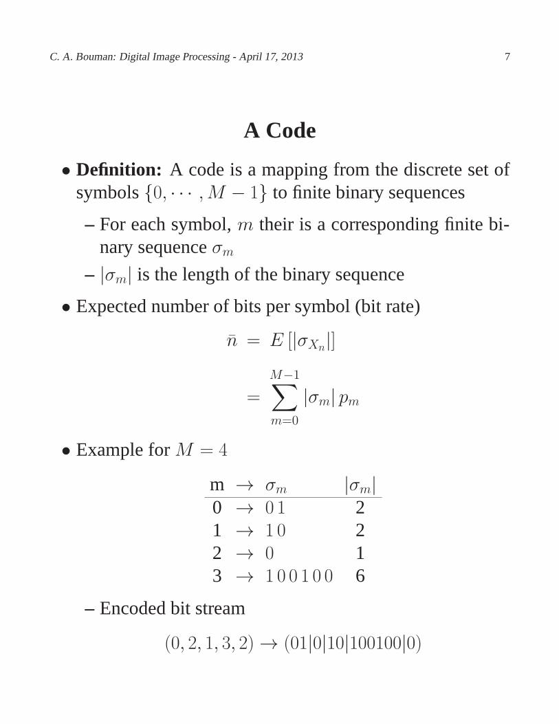
• Example forM = 4
m → σm |σm|0 → 0 1 21 → 1 0 22 → 0 13 → 1 0 0 1 0 0 6
– Encoded bit stream
(0, 2, 1, 3, 2)→ (01|0|10|100100|0)
C. A. Bouman: Digital Image Processing - April 17, 2013 8
Fixed versus Variable Length Codes
• Fixed Length Code -|σm| is constant for allm
• Variable Length Code -|σm| varies withm
• Problem
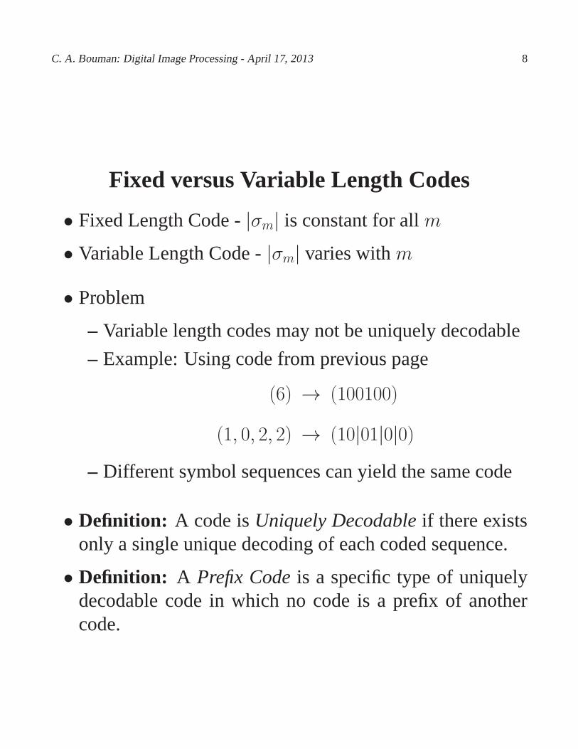
– Variable length codes may not be uniquely decodable
– Example: Using code from previous page
(6) → (100100)
(1, 0, 2, 2) → (10|01|0|0)
– Different symbol sequences can yield the same code
• Definition: A code isUniquely Decodableif there existsonly a single unique decoding of each coded sequence.
• Definition: A Prefix Codeis a specific type of uniquelydecodable code in which no code is a prefix of anothercode.
C. A. Bouman: Digital Image Processing - April 17, 2013 9
Lower Bound on Bit Rate
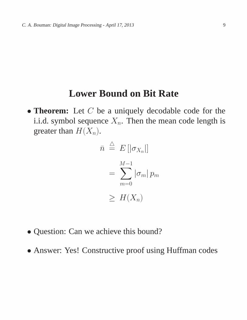
• Theorem: Let C be a uniquely decodable code for thei.i.d. symbol sequenceXn. Then the mean code length isgreater thanH(Xn).
n̄△= E [|σXn|]
=
M−1∑
m=0
|σm| pm
≥ H(Xn)
• Question: Can we achieve this bound?
• Answer: Yes! Constructive proof using Huffman codes
C. A. Bouman: Digital Image Processing - April 17, 2013 10
Huffman Codes
• Variable length prefix code⇒ Uniquely decodable
• Basic idea:
– Low probability symbols⇒ Long codes
– High probability symbols⇒ short codes
• Basic algorithm:
– Low probability symbols⇒ Long codes
– High probability symbols⇒ short codes
C. A. Bouman: Digital Image Processing - April 17, 2013 11
Huffman Coding Algorithm
1. Initialize list of probabilities with the probability ofeachsymbol
2. Search list of probabilities for two smallest probabilities,pk∗ andpl∗.
3. Add two smallest probabilities to form a new probability,pm = pk∗ + pl∗.
4. Removepk∗ andpl∗ from the list.
5. Addpm to the list.
6. Go to step 2 until the list only contains 1 entry
C. A. Bouman: Digital Image Processing - April 17, 2013 12
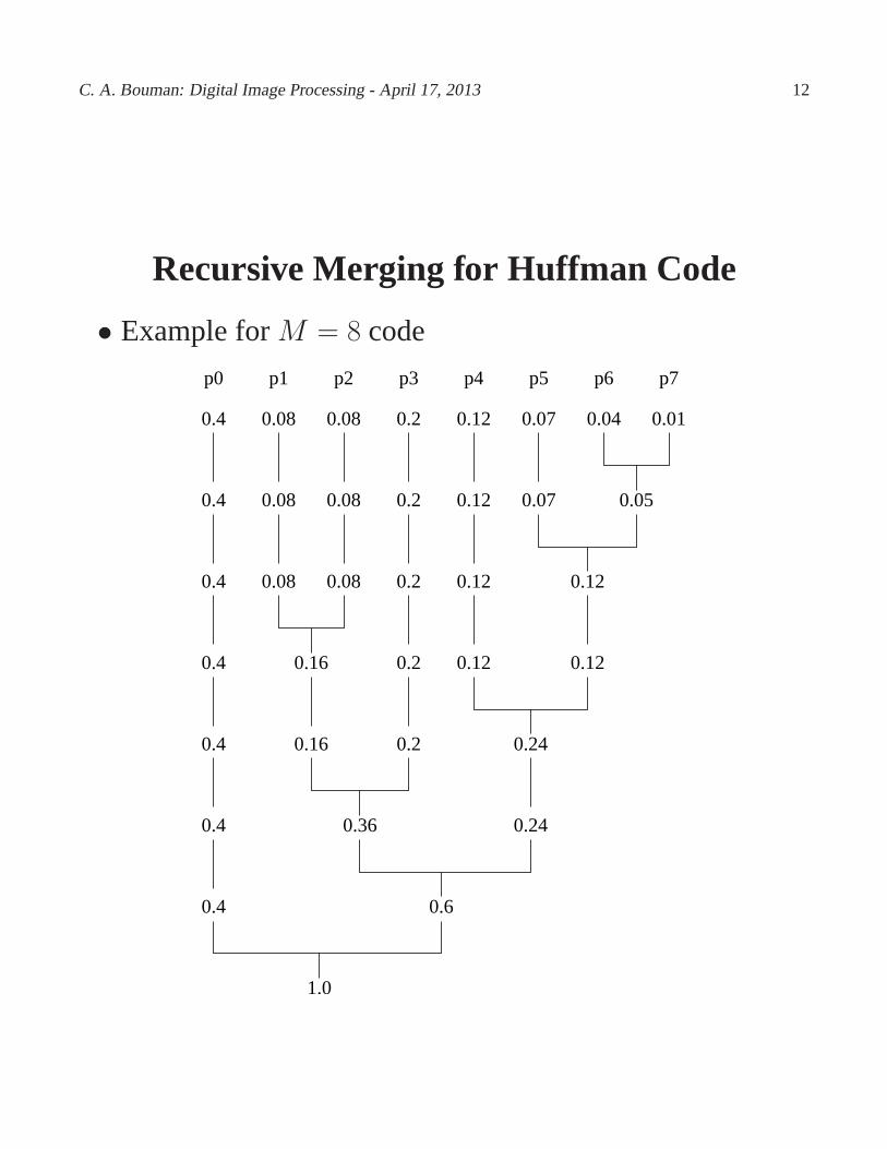
Recursive Merging for Huffman Code
• Example forM = 8 code
1.0
0.04 0.01
0.050.070.4 0.08 0.08 0.2 0.12
0.4 0.08 0.08 0.2 0.12 0.07
p1p0 p2 p3 p7p4 p5 p6
0.120.4 0.08 0.08 0.2 0.12
0.160.4 0.2 0.12 0.12
0.240.20.16
0.36
0.4
0.4 0.24
0.60.4
C. A. Bouman: Digital Image Processing - April 17, 2013 13
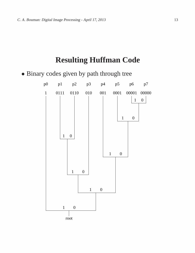
Resulting Huffman Code
• Binary codes given by path through tree
00000
p1p0 p2 p3 p7p4 p5 p6
1
1 0
root
1 0
1 0
01
1 0
1 0
1 0
0111 0110 010 001 0001 00001
C. A. Bouman: Digital Image Processing - April 17, 2013 14
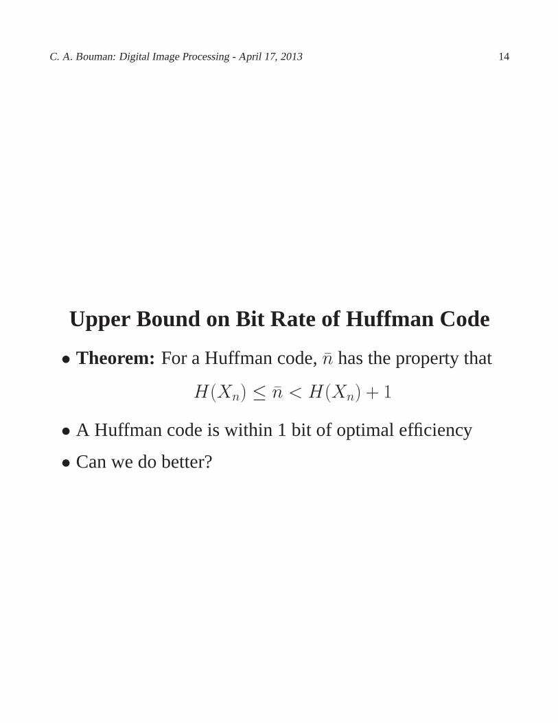
Upper Bound on Bit Rate of Huffman Code
• Theorem: For a Huffman code,̄n has the property that
H(Xn) ≤ n̄ < H(Xn) + 1
• A Huffman code is within 1 bit of optimal efficiency
• Can we do better?
C. A. Bouman: Digital Image Processing - April 17, 2013 15
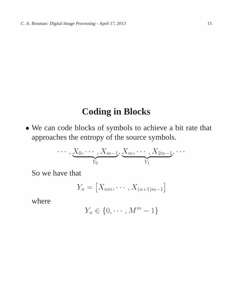
Coding in Blocks
• We can code blocks of symbols to achieve a bit rate thatapproaches the entropy of the source symbols.
· · · , X0, · · · , Xm−1︸ ︷︷ ︸Y0
, Xm, · · · , X2m−1︸ ︷︷ ︸Y1
, · · ·
So we have that
Yn =[Xnm, · · · , X(n+1)m−1
]
whereYn ∈ {0, · · · ,Mm − 1}
C. A. Bouman: Digital Image Processing - April 17, 2013 16
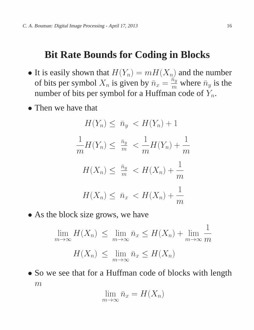
Bit Rate Bounds for Coding in Blocks
• It is easily shown thatH(Yn) = mH(Xn) and the numberof bits per symbolXn is given byn̄x =
n̄ym
wheren̄y is thenumber of bits per symbol for a Huffman code ofYn.
• Then we have that
H(Yn) ≤ n̄y < H(Yn) + 1
1
mH(Yn) ≤ n̄y
m<
1
mH(Yn) +
1
m
H(Xn) ≤ n̄ym
< H(Xn) +1
m
H(Xn) ≤ n̄x < H(Xn) +1
m
• As the block size grows, we have
limm→∞
H(Xn) ≤ limm→∞
n̄x ≤ H(Xn) + limm→∞
1
m
H(Xn) ≤ limm→∞
n̄x ≤ H(Xn)
• So we see that for a Huffman code of blocks with lengthm
limm→∞
n̄x = H(Xn)
C. A. Bouman: Digital Image Processing - April 17, 2013 17
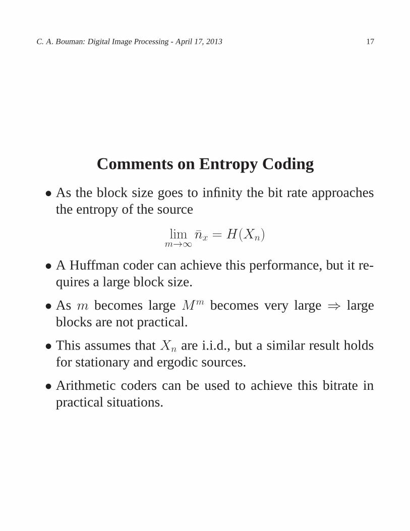
Comments on Entropy Coding
• As the block size goes to infinity the bit rate approachesthe entropy of the source
limm→∞
n̄x = H(Xn)
• A Huffman coder can achieve this performance, but it re-quires a large block size.
• As m becomes largeMm becomes very large⇒ largeblocks are not practical.
• This assumes thatXn are i.i.d., but a similar result holdsfor stationary and ergodic sources.
• Arithmetic coders can be used to achieve this bitrate inpractical situations.
C. A. Bouman: Digital Image Processing - April 17, 2013 18
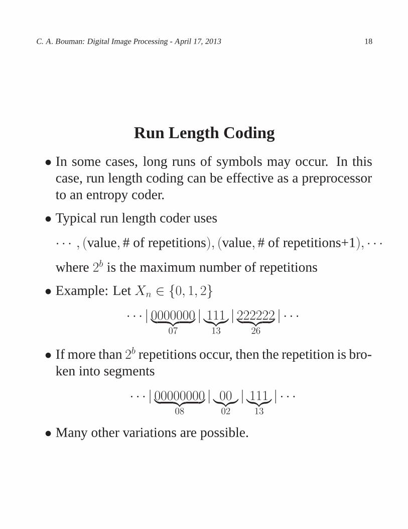
Run Length Coding
• In some cases, long runs of symbols may occur. In thiscase, run length coding can be effective as a preprocessorto an entropy coder.
• Typical run length coder uses
· · · , (value, # of repetitions), (value, # of repetitions+1), · · ·where2b is the maximum number of repetitions
• Example: LetXn ∈ {0, 1, 2}· · · | 0000000︸ ︷︷ ︸
07
| 111︸︷︷︸13
| 222222︸ ︷︷ ︸26
| · · ·
• If more than2b repetitions occur, then the repetition is bro-ken into segments
· · · | 00000000︸ ︷︷ ︸08
| 00︸︷︷︸02
| 111︸︷︷︸13
| · · ·
• Many other variations are possible.
C. A. Bouman: Digital Image Processing - April 17, 2013 19
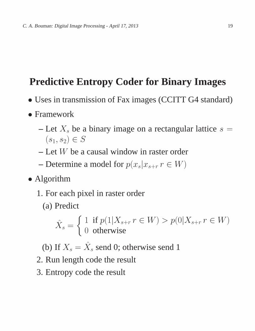
Predictive Entropy Coder for Binary Images
• Uses in transmission of Fax images (CCITT G4 standard)
• Framework
– Let Xs be a binary image on a rectangular lattices =(s1, s2) ∈ S
– LetW be a causal window in raster order
– Determine a model forp(xs|xs+r r ∈ W )
• Algorithm
1. For each pixel in raster order
(a) Predict
X̂s =
{1 if p(1|Xs+r r ∈ W ) > p(0|Xs+r r ∈ W )0 otherwise
(b) If Xs = X̂s send 0; otherwise send 1
2. Run length code the result
3. Entropy code the result
C. A. Bouman: Digital Image Processing - April 17, 2013 20
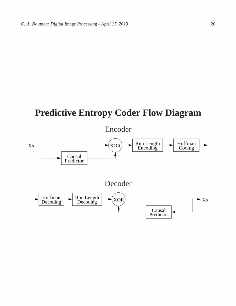
Predictive Entropy Coder Flow Diagram
Encoder
Causal
CodingHuffmanXs XOR Encoding
Run Length
Predictor
Decoder
DecodingHuffmanDecoding
Run Length
PredictorCausal
XsXOR
C. A. Bouman: Digital Image Processing - April 17, 2013 21
How to Choosep(xs|xs+r r ∈ W )?
• Non-adaptive method
– Select typical set of training images
– Design predictor based on training images
• Adaptive method
– Allow predictor to adapt to images being coded
– Design decoder so it adapts in same manner as encoder
C. A. Bouman: Digital Image Processing - April 17, 2013 22
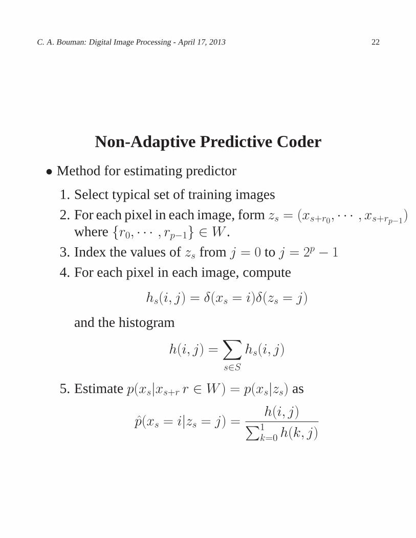
Non-Adaptive Predictive Coder
• Method for estimating predictor
1. Select typical set of training images
2. For each pixel in each image, formzs = (xs+r0, · · · , xs+rp−1)where{r0, · · · , rp−1} ∈ W .
3. Index the values ofzs from j = 0 to j = 2p − 1
4. For each pixel in each image, compute
hs(i, j) = δ(xs = i)δ(zs = j)
and the histogram
h(i, j) =∑
s∈Shs(i, j)
5. Estimatep(xs|xs+r r ∈ W ) = p(xs|zs) as
p̂(xs = i|zs = j) =h(i, j)
∑1k=0 h(k, j)
C. A. Bouman: Digital Image Processing - April 17, 2013 23
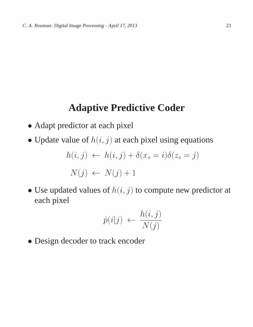
Adaptive Predictive Coder
• Adapt predictor at each pixel
• Update value ofh(i, j) at each pixel using equations
h(i, j) ← h(i, j) + δ(xs = i)δ(zs = j)
N(j) ← N(j) + 1
• Use updated values ofh(i, j) to compute new predictor ateach pixel
p̂(i|j) ← h(i, j)
N(j)
• Design decoder to track encoder
C. A. Bouman: Digital Image Processing - April 17, 2013 24
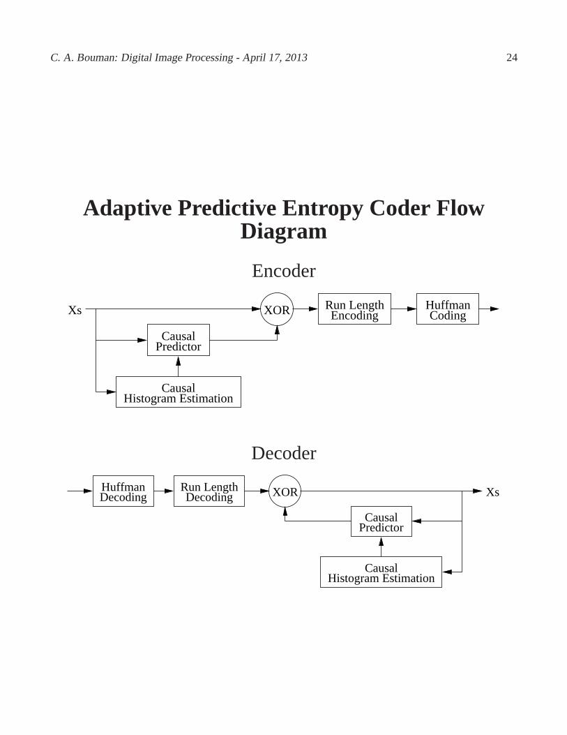
Adaptive Predictive Entropy Coder FlowDiagram
Encoder
Histogram Estimation
CodingHuffmanXs XOR Encoding
Run Length
PredictorCausal
Causal
Decoder
DecodingHuffmanDecoding
Run Length
PredictorCausal
CausalHistogram Estimation
XsXOR
C. A. Bouman: Digital Image Processing - April 17, 2013 25
Lossy Source Coding
• Method for representing discrete-space signals with min-imum distortion and bit-rate
• Outline
– Rate-distortion theory
– Karhunen-Loeve decorrelating Transform
– Practical coder structures
C. A. Bouman: Digital Image Processing - April 17, 2013 26
Distortion
• Let X andZ be random vectors inIRM . Intuitively, X isthe original image/data andZ is the decoded image/data.
Assume we use the squared error distortion measure givenby
d(X, Y ) = ||X − Z||2
Then the distortion is given by
D = E [d(X, Y )] = E[
||X − Z||2]
• This actually applies to any quadratic norm error distor-tion measure since we can define
X̃ = AX and Z̃ = AZ
SoD̃ = E
[∣∣∣∣X̃ − Z̃
∣∣∣∣2]
= E[
||X − Z||2B]
whereB = AtA.
C. A. Bouman: Digital Image Processing - April 17, 2013 27
Lossy Source Coding: Theoretical Framework
• Notation for source coding
Xn ∈ IRM for 0 ≤ n < N - a sequence of i.i.d. randomvectors
Y ∈ {0, 1}K - aK bit random binary vector.
Zn ∈ IRM for 0 ≤ n < N - the decoded sequence ofrandom vectors.
X (N) = (X0, · · · , XN−1)
Z(N) = (Z0, · · · , ZN−1)
– Encoder function:Y = Q(X0, · · · , XN−1)
– Decoder function:(Z0, · · · , ZN−1) = f (Y )
• Resulting quantities
Bit-rate= KN
Distortion=1
N
N−1∑
n=0
E[
||Xn − Zn||2]
• How do we chooseQ(·) to minimize the bit-rate and dis-tortion?
C. A. Bouman: Digital Image Processing - April 17, 2013 28
Differential Entropy
• Notice that the information contained in a Gaussian ran-dom variable is infinite, so the conventional entropyH(X)is not defined.
• Let X be a random vector taking values inIRM with den-sity functionp(x). Then we define the differential entropyof X as
h(X) = −∫
x∈IRM
p(x) log2 p(x)dx
= −E [log2 p(X)]
h(X) has units of bits
C. A. Bouman: Digital Image Processing - April 17, 2013 29
Conditional Entropy and Mutual Information
• Let X andY be a random vectors taking values inIRM
with density functionp(x, y) and conditional densityp(x|y).• Then we define the differential conditional entropy ofX
givenY as
h(X|Y ) = −∫
x∈IRM
∫
x∈IRM
p(x, y) log2 p(x|y)
= −E [log2 p(X|Y )]
• The mutual information betweenX andY is given by
I(X ;Y ) = h(X)− h(X|Y ) = I(Y ;X)
• Important: The mutual information is well defined forboth continuous and discrete random variables, and it rep-resents the reduction in uncertainty ofX givenY .
C. A. Bouman: Digital Image Processing - April 17, 2013 30
The Rate-Distortion Function
• Define/Remember:
– LetX0 be the first element of the i.i.d. sequence.
– LetD ≥ 0 be the allowed distortion.
• For a specific distortion,D, the rate is given by
R(D) = infZ
{I(X0;Z) : E
[||X0 − Z||2
]≤ D
}
where the infimum (i.e. minimum) overZ is taken overall random variablesZ.
• Later, we will show that for a given distortion we can finda code that gets arbitrarily close to this optimum bit-rate.
C. A. Bouman: Digital Image Processing - April 17, 2013 31
Properties of the Rate-Distortion Function
• Properties ofR(D)
– R(D) is a monotone decreasing function ofD.
– If D ≥ E[
||X0||2]
, thenR(D) = 0
– R(D) is a convex function ofD
C. A. Bouman: Digital Image Processing - April 17, 2013 32
Shannon’s Source-Coding Theorem
• Shannon’s Source-Coding Theorem:For anyR′ > R(D) andD′ > D there exists a sufficientlylargeN such that there is an encoder
Y = Q(X0, · · · , XN−1)
which achieves
Rate=K
N≤ R′
and
Distortion=1
N
N−1∑
n=0
E[
||Xn − Zn||2]
≤ D′
• Comments:
– One can achieve a bit rate arbitrarily close toR(D) ata distortionD.
– Proof is constructive (but not practical), and uses codesthat are randomly distributed in the spaceIRMN of sourcesymbols.
C. A. Bouman: Digital Image Processing - April 17, 2013 33
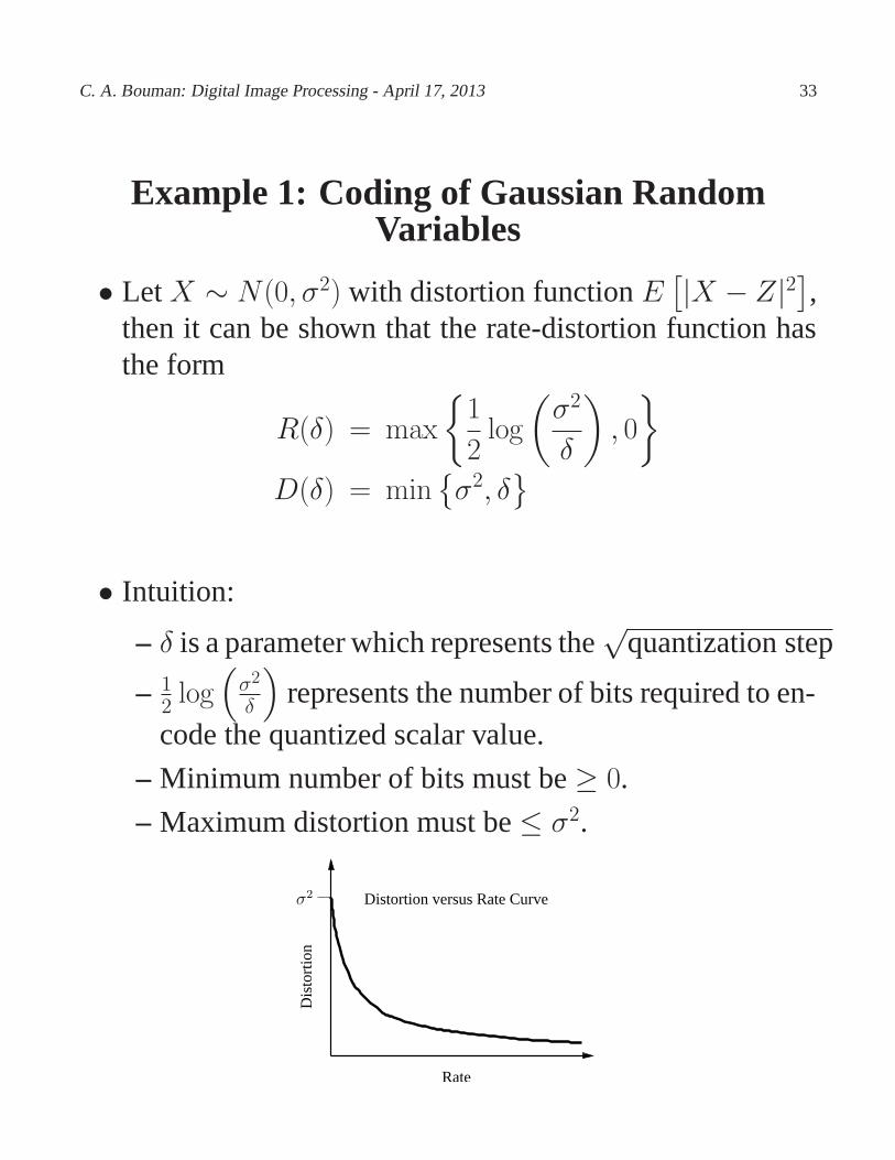
Example 1: Coding of Gaussian RandomVariables
• LetX ∼ N(0, σ2) with distortion functionE[|X − Z|2
],
then it can be shown that the rate-distortion function hasthe form
R(δ) = max
{1
2log
(σ2
δ
)
, 0
}
D(δ) = min{σ2, δ
}
• Intuition:
– δ is a parameter which represents the√
quantization step
– 12 log
(σ2
δ
)
represents the number of bits required to en-code the quantized scalar value.
– Minimum number of bits must be≥ 0.
– Maximum distortion must be≤ σ2.
Distortion versus Rate Curve
Dis
tort
ion
Rate
σ2
C. A. Bouman: Digital Image Processing - April 17, 2013 34
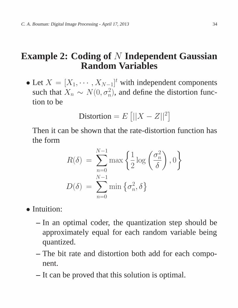
Example 2: Coding ofN Independent GaussianRandom Variables
• Let X = [X1, · · · , XN−1]t with independent componentssuch thatXn ∼ N(0, σ2
n), and define the distortion func-tion to be
Distortion= E[||X − Z||2
]
Then it can be shown that the rate-distortion function hasthe form
R(δ) =
N−1∑
n=0
max
{1
2log
(σ2n
δ
)
, 0
}
D(δ) =
N−1∑
n=0
min{σ2n, δ
}
• Intuition:
– In an optimal coder, the quantization step should beapproximately equal for each random variable beingquantized.
– The bit rate and distortion both add for each compo-nent.
– It can be proved that this solution is optimal.
C. A. Bouman: Digital Image Processing - April 17, 2013 35
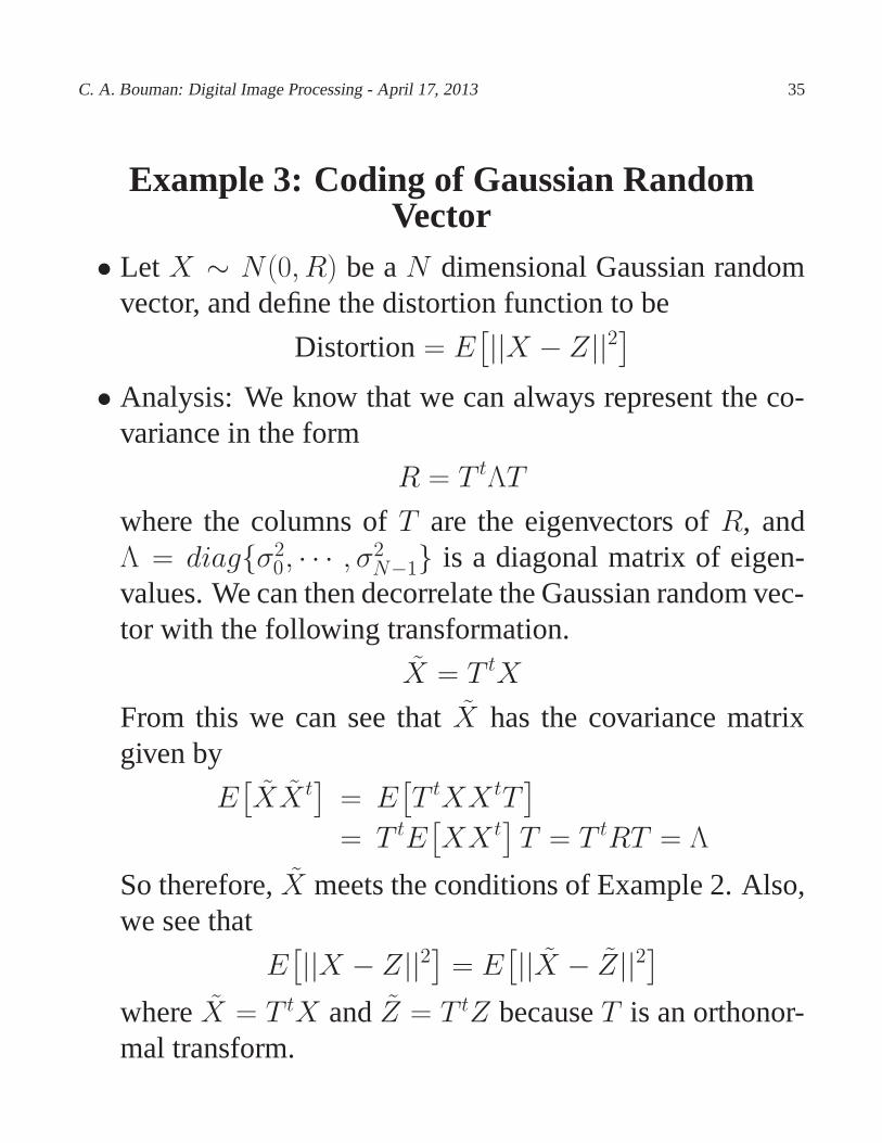
Example 3: Coding of Gaussian RandomVector
• Let X ∼ N(0, R) be aN dimensional Gaussian randomvector, and define the distortion function to be
Distortion= E[||X − Z||2
]
• Analysis: We know that we can always represent the co-variance in the form
R = T tΛT
where the columns ofT are the eigenvectors ofR, andΛ = diag{σ2
0, · · · , σ2N−1} is a diagonal matrix of eigen-
values. We can then decorrelate the Gaussian random vec-tor with the following transformation.
X̃ = T tX
From this we can see that̃X has the covariance matrixgiven by
E[X̃X̃ t
]= E
[T tXX tT
]
= T tE[XX t
]T = T tRT = Λ
So therefore,X̃ meets the conditions of Example 2. Also,we see that
E[||X − Z||2
]= E
[||X̃ − Z̃||2
]
whereX̃ = T tX andZ̃ = T tZ becauseT is an orthonor-mal transform.
C. A. Bouman: Digital Image Processing - April 17, 2013 36
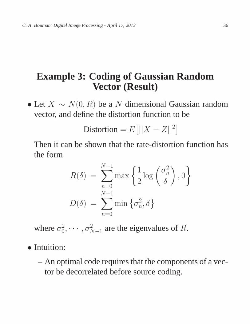
Example 3: Coding of Gaussian RandomVector (Result)
• Let X ∼ N(0, R) be aN dimensional Gaussian randomvector, and define the distortion function to be
Distortion= E[||X − Z||2
]
Then it can be shown that the rate-distortion function hasthe form
R(δ) =
N−1∑
n=0
max
{1
2log
(σ2n
δ
)
, 0
}
D(δ) =
N−1∑
n=0
min{σ2n, δ
}
whereσ20, · · · , σ2
N−1 are the eigenvalues ofR.
• Intuition:
– An optimal code requires that the components of a vec-tor be decorrelated before source coding.
C. A. Bouman: Digital Image Processing - April 17, 2013 37
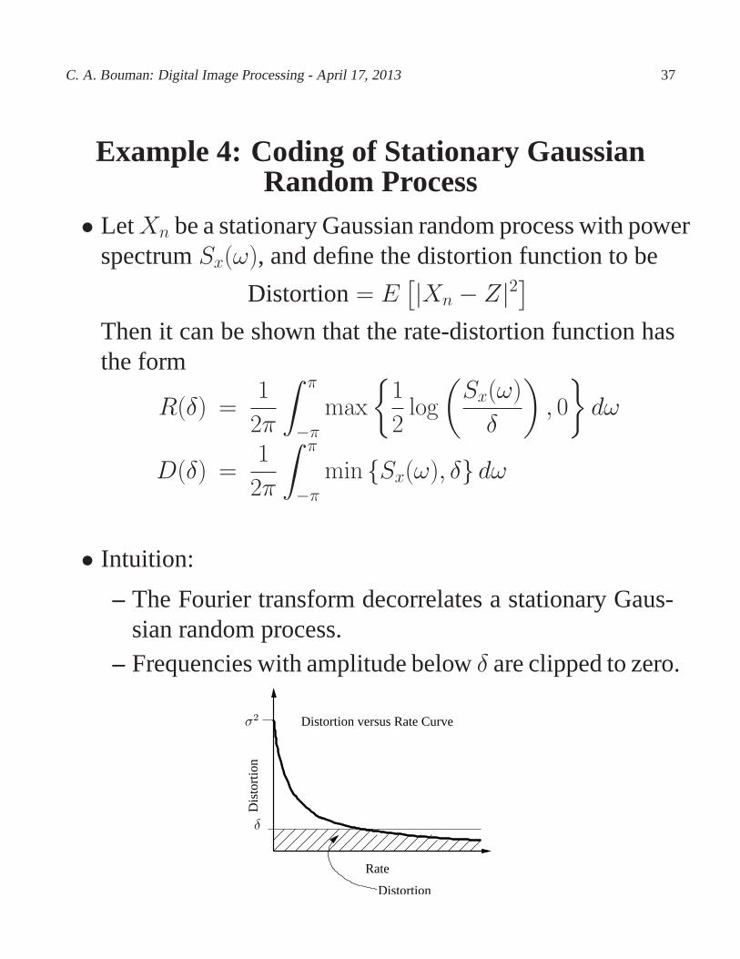
Example 4: Coding of Stationary GaussianRandom Process
• LetXn be a stationary Gaussian random process with powerspectrumSx(ω), and define the distortion function to be
Distortion= E[|Xn − Z|2
]
Then it can be shown that the rate-distortion function hasthe form
R(δ) =1
2π
∫ π
−πmax
{1
2log
(Sx(ω)
δ
)
, 0
}
dω
D(δ) =1
2π
∫ π
−πmin {Sx(ω), δ} dω
• Intuition:
– The Fourier transform decorrelates a stationary Gaus-sian random process.
– Frequencies with amplitude belowδ are clipped to zero.
Distortion versus Rate Curve
Dis
tort
ion
Rate
Distortion
δ
σ2
C. A. Bouman: Digital Image Processing - April 17, 2013 38
The Discrete Cosine Transform (DCT)
• DCT (There is more than one version)
F (k) =1√N
N−1∑
n=0
f (n) c(k) cos
(π(2n + 1)k
2N
)
where
c(k) =
{1 k = 0√2 k = 1, · · · , N − 1
}
• Inverse DCT (IDCT)
f (n) =1√N
N−1∑
k=0
F (k) c(k) cos
(π(2n + 1)k
2N
)
• Comments:
– In this form, the DCT is an orthonormal transform. Soif we define the matrixF such that
Fn,k = c(k) cos
(π(2n + 1)k
2N
)
,
thenF−1 = FH where
F−1 =[F t
]∗= FH
– Takes andN -point real valued signal to anN -pointreal valued signal.
C. A. Bouman: Digital Image Processing - April 17, 2013 39
Relationship Between DCT and DFT
• Let us define the padded version off (n) as
fp(n) =
{f (n) 0 ≤ n ≤ N − 10 N ≤ n ≤ 2N − 1
and its2N -point DFT denoted byFp(k). Then the DCTcan be written as
F (k) =c(k)√N
N−1∑
n=0
f (n) cos
(π(2n + 1)k
2N
)
=c(k)√N
N−1∑
n=0
f (n)Re{
e−j2π(2n+1)k
2N e−jπk2N
}
=c(k)√NRe
{
e−jπk2N
2N−1∑
n=0
fp(n)e−j 2π(2n+1)k
2N
}
=c(k)√NRe
{
e−jπk2NFp(k)
}
=c(k)√N
(
Fp(k)e−j πk
2N + Fp(k)e+j πk
2N
)
=c(k)e−j
πk2N
√N
(
Fp(k) +(
Fp(k)e−j 2πk2N
)∗)
C. A. Bouman: Digital Image Processing - April 17, 2013 40
Interpretation of DFT Terms
• Consider the inverse DCT for each of the two terms
Fp(k)⇔ fp(n)
• DCT{fp(n)} ⇒ Fp(k)
• DCT{fp(−n +N − 1)} ⇒(
Fp(k)e−j 2πk2N
)∗
• Simple example forN = 4
f (n)
= [f (0), f (1), f (2), f (3)]
fp(n)
= [f (0), f (1), f (2), f (3), 0, 0, 0, 0]
fp(−n+N−1)= [0, 0, 0, 0, f (3), f (2), f (1), f (0)]
f (n) + fp(−n+N−1)= [f (0), f (1), f (2), f (3), f (3), f (2), f (1), f (0)]
C. A. Bouman: Digital Image Processing - April 17, 2013 41
Relationship Between DCT and DFT(Continued)
• So the DCT is formed by2N -point DFT off (n)+f (−n+N − 1).
F (k) =c(k)e−j
πk2N
√N
DFT2N {f (n) + f (−n +N − 1)}