Ubiquitous Superconducting Sensors in Cosmology

Hsiao-Mei (Sherry) Cho

National Institute of Standards and Technology, Boulder, CO, USA

Friday March 5, 2010

Department of Physics

National Chung-Hsin University, TaiChung, Taiwan

卓筱梅

OutlineIntroduction

Part I: Looking for CMB polarization

Part II: Help wanted

● Transition Edge Sensor (TES) ● Superconducting QUantum Interference Device (SQUID)

● Polarimeter design and results ● Projects

Future plans

● Superconductivity● Thermodynamics ● Material science

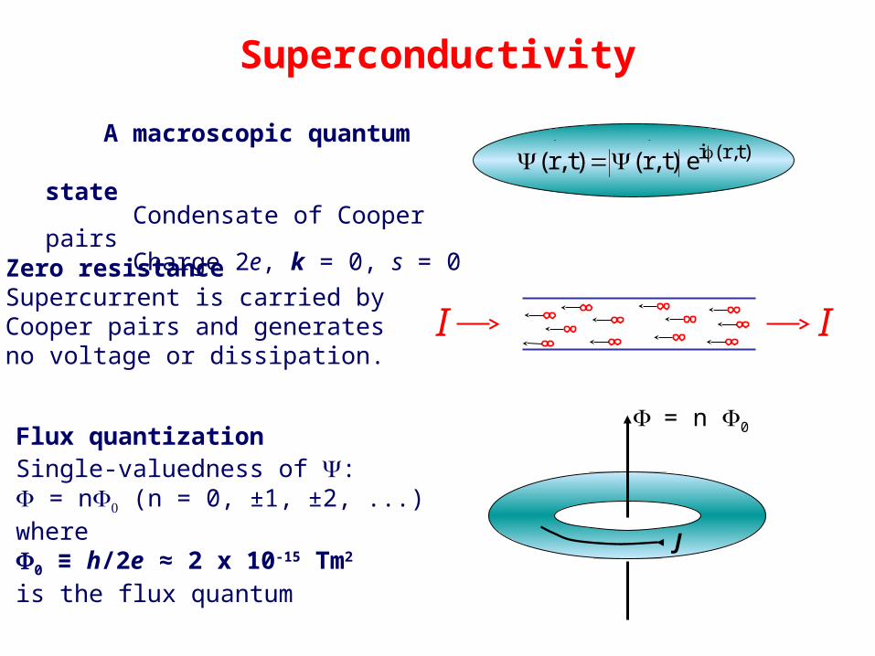
Superconductivity

A macroscopic quantum state Condensate of Cooper pairs Charge 2e, k = 0, s = 0

)t,r(ie)t,r()t,r(

I I

Zero resistanceSupercurrent is carried by Cooper pairs and generatesno voltage or dissipation.

= n 0

J

Flux quantization Single-valuedness of : = n (n = 0, ±1, ±2, ...) where 0 ≡ h/2e ≈ 2 x 10-15 Tm2

is the flux quantum

Typical R vs T

T

R

Josephson Tunneling

Brian Josephson 1962Cooper pairs tunnel through a barrier

V

I

I

Oxidized Nb film

Nb film

I

Superconductor 1 Superconductor 2

~ 20 Å

Insulatingbarrier

I

V

V

I

I = I0 sin = 1 – 2

d/dt = 2eV/ħ = 2V/0

1 2

The dc Superconducting Quantum Interference Device

IV

0 1 2 0

V

Current-voltage (I-V) characteristic modulated by magnetic flux  Period one flux quantum 0 = h/2e ≈ 2 x 10-15 T m2

DC SQUID

Two Josephson junctions on a superconducting ringI

V

n0

(n+1/2)0

VV

Ib

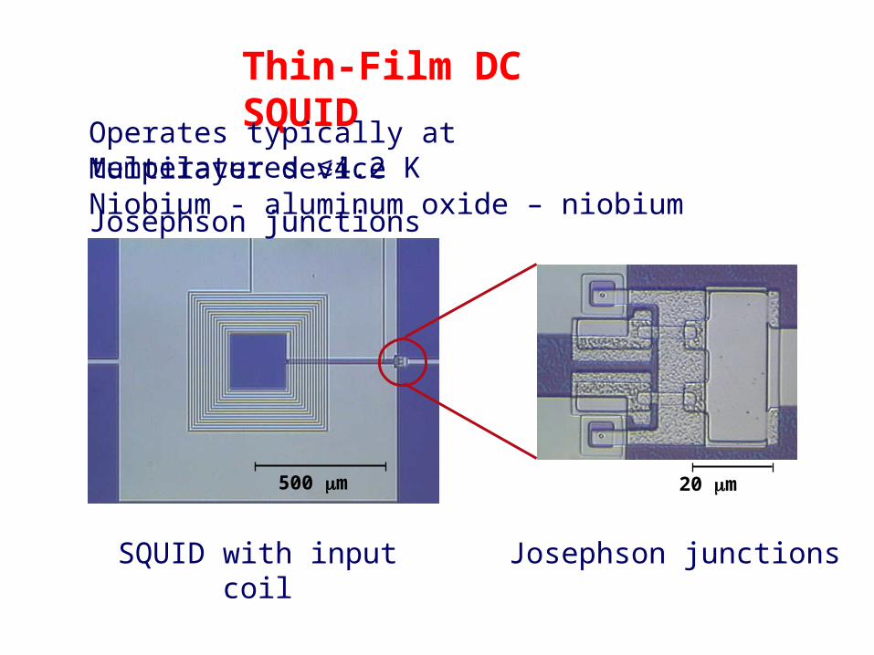
Thin-Film DC SQUID

SQUID with input coil Josephson junctions

500 m 20 m

Operates typically at temperatures ≲4.2 KMultilayer device Niobium - aluminum oxide – niobium Josephson junctions

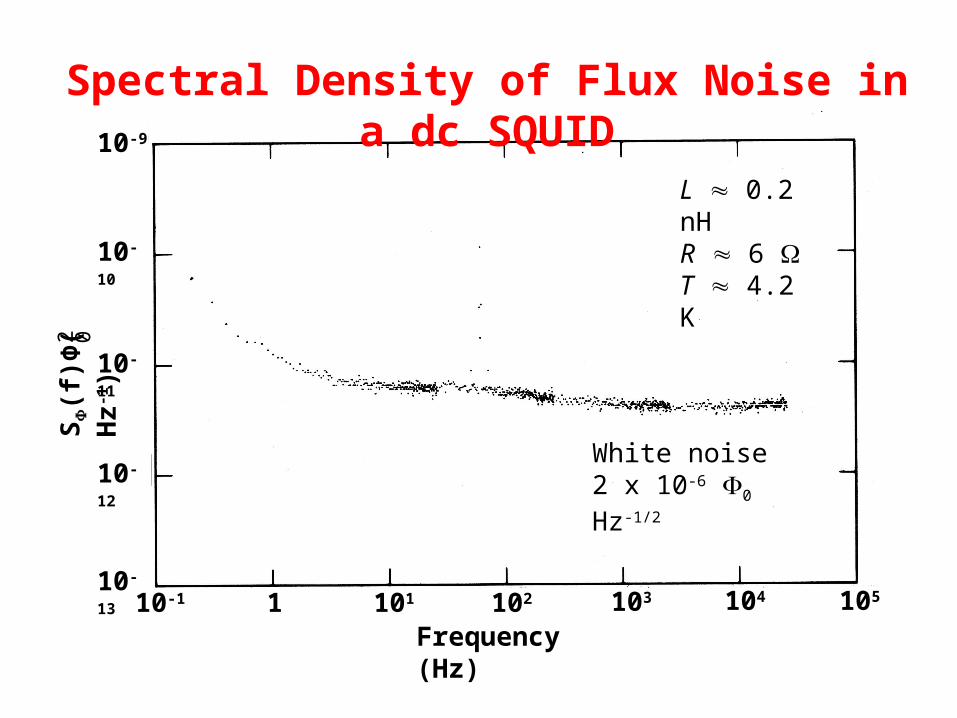
Frequency (Hz)10-1 1 101 102 103 104 105

White noise2 x 10-6 0 Hz-1/2

L 0.2 nHR 6 T 4.2 K

Spectral Density of Flux Noise in a dc SQUIDS

(f

) (

H

z-1)

2 0Φ

10-9

10-10

10-11

10-12

10-13

Magnetic Fields

1 femtotesla

tesla

10-16

10-10

10-8

10-6

10-4

10-12

10-14

10-2

1

Earth’s field

Urban noise

Car at 50 m

Human heart

Fetal heart

Human brain response

SQUID magnetometer

Conventional MRI

Voltage-Biased Transition-Edge Sensor (TES) Bolometer

SQUID

250 mK

TES

Weakthermal link

Optical absorber

T

R

• Electrothermal feedback: fast, linear response• Low power dissipation (~1 nW)• Sensitivity limited by fluctuations in the photon arrival rate

Ptotal = Popt + Pelc = constant

Looking for CMB polarization

Courtesy of WMAP

The universe we know

CMB = cosmic microwave background

Gravity waves make a uniform temperature distribution appear hotter in one direction (anisotropy), resulting in polarization.

We consider the primordial plasma as an array of test masses in a giant gravitational radiation detector

Anisotropies from gravitational waves

Simulations from SPIDER collaborationSimulations from SPIDER collaboration

No gravity waves

• Simulation of CMB polarization signal with no gravity waves

• The “curl” of the polarization is zero.

Gravity wave signature

No TensorGravity waves!!!

Simulations from SPIDER collaborationSimulations from SPIDER collaboration

Gravity wave signature

• Simulation of CMB polarization signal with gravity waves

• The “curl” of the polarization is nonzero: gravity waves!

BICEP

The state of the field

100 GHz

150 GHz

The state of the fieldl(l+

1)C

l/2 (

K2 )

… but orders of magnitude improvement inmapping speed needed.

TES for CMB polarimetry

B.A. Benson L. E. Bleem C. L. Chang A.T. Crites W. Everett J. McMahon J. Mehl S.S. Meyer J.E. Carlstrom

J.A. Beall D. Becker J. Britton G.C. Hilton J. Hubmayr K.D. IrwinM.D. Niemack K.W. Yoon

J.E. Austermann N.W. Halverson J.W.HenningS.M. Simon

J. W. Appel L. P. Parker T. Essinger-Hileman Y. ZhaoS. T. Staggs C. Visnjic

CU-BoulderPrinceton University

University of Chicago

OMT design

CPW tomicrostrip transition

TES

Heater

Gold meander

150 GHz CMB polarimeter

fabricated at NIST

Components designed by NIST, CU-Boulder, University of Chicago and Princeton University

5 mm

TES A

TES BTES D

Si Tbath = 0.3K

SiN

Nb

MoCu TESTc ~ 530 mK

Filter design

4/

OMT design

CPW to microstrip transition

smooth transition from CPW (~70 Ohm) to microstrip (~10 Ohm)

Microstrip stub filters design

/4 shorted stub bandpass filters

Stepped impedance low-pass filters

Lossy gold absorber

Nb-to-Au transition is well-matched --- low reflection loss

Voltage-Biased Transition-Edge Sensor (TES) Bolometer

SQUID

250 mK

TES

Weakthermal link

Optical absorber

T

R

• Electrothermal feedback: fast, linear response• Low power dissipation (~1 nW)• Sensitivity limited by fluctuations in the photon arrival rate

Ptotal = Popt + Pelc = constant

Optical power vs Tbath

Ptotal = Popt + Pelec (70% Rn)

Noise performance

(4kGTC2)1/2

FTS bandpass measurements

100 120 140 160 180 200

0

10

20

30

40

TES A TES B simulation:

CMB5 simulation:

CMB4

Resp

onse

(arb

. unit

)

Frequency (GHz)100 120 140 160 180 200

-5

0

5

10

15

20

25

30

35

40 TES A TES B simulation

Resp

onse

(arb

. unit

)

Frequency (GHz)

Run 1: 5 GHz shift due to assuming er = 4.2

Run 1 Run 2 Run 3

5 GHz

Run 2:After correction,

measured and predicted bandpass (127-163 GHz)

agree

Run 3: Measured and predicted bandpass (127-159GHz)

agree

Backshortwafer

Polarimeterwafer

CMB polarization: possible pixel schematicAu plated Si feed horns

5 mm

2 mm

Prototype array

Si feedhorns

4 inch

Future projects require 7 wafers, ~ 1300 TESs

Instruments in development

Atacama B-mode Search(ABS)

South Pole TelescopePolarimeter

SPTPol

Atacama Cosmology Telescope Polarimeter

ACT-pol

Atacama, Chile2012

South Pole2012

Atacama, Chile2010

Help Wanted

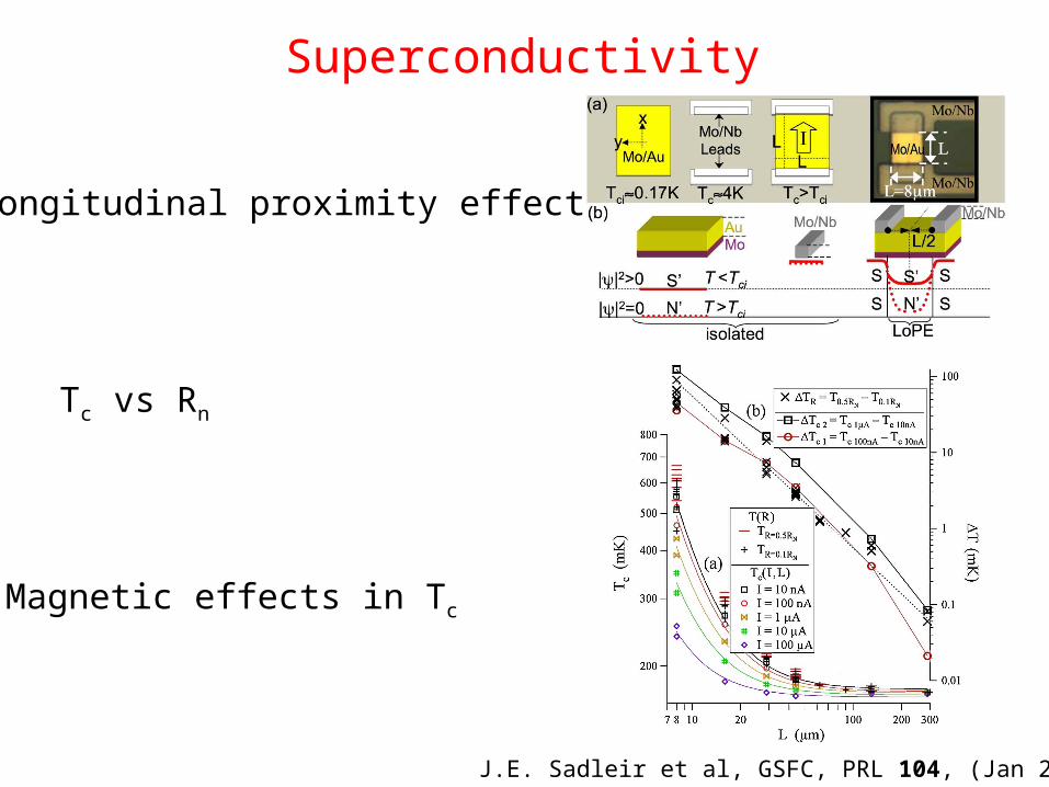
Superconductivity

Longitudinal proximity effects

Tc vs Rn

J.E. Sadleir et al, GSFC, PRL 104, (Jan 2010)

Magnetic effects in Tc

Thermodynamics

In each pixel

P = K (Tcn – Tbath

n)

G = dP/dTc

120

μm

TES Intrinsic time constant: tes = 50 μsTES + Bling time constant: 0 = C/G = 20 msDecoupling time: int = 400 ms

UC-Berkeley design

350 m

NIST design

Cu bank500 nm

Mo/Cu TES

Nb leads

TES Intrinsic time constant: tes = 7-10 ms

UC-Berkeley:

NIST:

0 = C/G where C is heat capacity

Material Science

Stress in thin films Damaged suspended SiN membrane Change Tc of TES Curve Si wafer

Loss in dielectric material

Shift bandpass Lower efficiency

High frequency leak

100 200 300 400-5

0

5

10

15

20

25

30

35

40

TES A TES B simulation

Res

pons

e (a

rb. u

nit)

Frequency (GHz)

High frequency leak

Unfortunately we have not figured out the cause yet.

Continue detailed optical and dark characterizations of CMB prototype pixels through summer

Finish measurements of 145 GHz Si feed; iterate on design

Extend existing design concept to 90/220 GHz

Si feed array (with 3” monolithic detector array) soon.

240 single-pixel polarimeters for ABS (deploy to Atacama in early 2010)

6” monolithic focal planes (~640 pixels) delivery for SPTpol & ACTpol by late 2011.

Future Plans

Thank you for your attention!!