1

UDEAGHA .C. EMEKA

BUDGET DEFICIT – INTEREST RATE

NEXUS IN NIGERIA:

SOCIAL SCIENCES

ECONOMICS

Okeke,chioma m

Digitally Signed by: University of Nigeria,

Nsukka

DN : CN = okeke,chioma m

O= University of Nigeria, Nsukka

OU = Innovation Centre

2

UNIVERSITY OF NIGERIA, NSUKKA

DEPARTMENT OF ECONOMICS

BUDGET DEFICIT – INTEREST RATE NEXUS IN

NIGERIA:

M.SC PROJECT PROPOSAL

BY

UDEAGHA .C. EMEKA PG/MSc/08/48408

SUPERVISOR: PROF. N. I. IKPEZE

3

CHAPTER ONE

INTRODUCTION

1.1 Background of the Study

Since the mid 1970s there has been much empirical and theoretical work about the effects

of government deficit on real economic activity in Nigeria and the rest of the world. A

good number of researchers have focused on testing the Ricardian equivalence.

According to David Ricardo, budget deficit does not matter, because an increase in

government deficit is effectively equivalent to a future increase in tax liabilities. Taking

into account that lower taxation in the present is offset by higher taxation in the future, it

means that budget deficits do not influence the macroeconomic variables. Authors such

as Barro (1974, 1987), Evans (1987), Darrat (1990) Beard and McMillan (1991) and

Cheng (1998) support the Barro – Ricardo view that government deficits have no impact

on key macroeconomic variables.

However, in the Keynes proposition some authors such as Bovenberg (1998),

Laumas (1989), Dua (1993) and others think otherwise, stating that budget deficits do

affect several, key macroeconomic variables, particularly real output, inflation, money

supply, interest rate and current account. Despite all the facts given by the Ricardian

equivalence in supporting the theory, it still remains an issue of controversy. In response

to these controversies, so many theoretical and empirical models have been examined in

checking the relationship in the first world economies and less developed economies and

the decision reached from these studies vary for the United State of America (USA)

alone, Gale and Orszag (2003) count about 30 studies that robustly find insignificant or

negative effects of budget deficits on interest rate about 30 studies do not. Given this

heterogeneity in some empirical literature, Bernheim (1989) concludes that it is easy to

cite a large number of studies that support any conceivable position. However, those who

are skeptical of the theoretical explanation as regards the theories are dependent on the

theoretical models to translate the relationship from empirical evidence.

So many authors such as Easterly and Schmidt – Hebbel in their own way also

argued that the relationship between budget deficits and interest rates is a complex one

because countries finance their deficits different ways. On the one hand under a repressed

financial sector, taxes on financial assets are a major source of revenue for the

4

government. On the other hand in a liberalized financial system where government

finances its deficits via domestic borrowing, public sector will compete with the private

sector for loans putting upward pressure on interest rates. The world bank (1993) opined

that in economies where financial markets are not repressed, higher deficit financed by

domestic debt increase domestic real interest rate when external borrowing is not

possible. Although if financial markets are integrated with world capital market higher

domestic borrowing results in international capital inflows and higher foreign debt, thus

the impact of domestic interest rate will not be much, more over in countries where

financial markets are repressed given a fixed nominal interest rate budget deficit raise

inflation resulting in a repressed (even negative) real interest rate as opposed by

Ricardian Equivalence Hypothesis of Barro (1974).

Given all these controversies surrounding the exact relationship between budget

deficits and interest rate and particularly given that the priorities of Nigeria include

amongst others making the country one of the largest twenty (20) economies in the world

by the year 2020 motivated this study.

1.2 Statement of Research Problem

Although it is one of the most studied issues in macroeconomics, it still remains a subject

of debate whether budget deficits affect interest rate and if so under what conditions.

However, so many papers have examined this crucial relationship for the growing

economies of the world and yet most pertinent conclusion from all of these work remain

the heterogeneity of their findings and because so many models and findings of the

economies exit, the findings offer several lots of arguments about the contact between

budget deficit and interest rate regarding its interaction, effects, magnitude or degree,

significance or insignificance as the case may be.

Budget deficit in Nigeria witnessed a little swing since early 1990s. It was -N7,

414.3m in 1991 and rose to –N53, 233.5m in 1993 and frog leaped to -N70, 270.6m in

1994. Between 1999 and 2008 budget deficit were –N133, 389.2m, -N285, 104.7m, -

N108,777.3m, -N221, 048.9m, -N301, 401.6m, -N202, 724.7m, -N172, 601.3m, -N161,

406.3m, -N101, 397.5m, -N117, 237.1m, -N47,378.50m respectively.

Interest rate rose from 27.7 in 1990 to all high of 36.09 in 1993 and thereafter declined

nose-dived to 21.0 in 1994. This represents 41.9% decline within period of one year.

5

Between 1999 and 2008 interest rate were 27.19, 21.55, 21.34, 30.19, 22.88, 20.82,

19.47, 18.70, 18.24 and 21.18 respectively.

Figure 1: Budget Deficit Vs Interest Rate.

Despite and given the relationship between budget deficit and interest rate the

alleged interactions between the two variables in the economy of Nigeria are still not

obvious from the trend evidence and this remains unclear despite the fact that this study

has already been investigated intensely. Arguably, this inconclusiveness originates from

the composition of composed kind of empirical studies, considering different data and

estimation techniques used in Nigeria and other various economies of the world.

Most of the studies reviewed were cross-country based analysis and thus produce

mixed results which give credence to country specific study because of country

peculiarities. In all of these it made it difficult in having general consensus as to the exact

relationship between both investigating macro economic variables, especially in

emerging economies such as Nigeria. To overcome this problem, this study will focus on

Nigeria to know the exact relationship between budget deficit and interest rate in Nigeria.

Other studies that were country specific like that of Obi and Nuruden (2008) and

Chimobi and Igwe (2010) all in Nigeria employed VAR model and Granger Causality

6

test without determining the optimum lag length of the model. According to Gujarati and

Sangeeta (2007) these two models are sensitive to lag length. Thus, to overcome this

problem, we use the AIC, SBC and minimum R2

criteria to determine the optimum lag

length. In addition, we shall use the impulse response function and variance

decomposition to determine the effect of shocks in the model cause by budget deficit.

1.3 Objective of the Study

The broad objective of the work is to examine and show the existing relationship between

budget deficit and interest rate in Nigeria. Some of the specific objectives are:

i. To ascertain whether or not budget deficit has an interaction with interest rate

in the Nigerian economy.

ii. To determine the direction of the interaction between budget deficit and

interest rate in Nigeria.

1.4 Statement of Hypothesis

In line with the preceding objectives, the hypotheses for the study are developed thus:

i. Budget deficit has no significant interaction with interest rate in Nigeria

ii. There is no direction of interaction between budget deficit and interest rate in

Nigeria.

1.5 Significance of the Study

This study will benefit both policy makers and investors in Nigeria. The knowledge of

the nature of the relationships between budget deficit and interest rate will help policy

makers in the following ways:

To know the appropriate monetary-fiscal policy mix.

To know the optimum deficit financing to use

Whether budget deficit interacts with interest rate thereby reducing savings, and

capital formation, if so, then policy makers can design ways through which

individuals can adjust their savings behavior taking cognizance of fiscal policy.

To benefit investors in managing their investment opportunities.

7

1.6 Scope of the Study

This study covered Federal Government budget deficit and interest rate for the period

1979-2009 in Nigeria.

8

CHAPTER TWO

LITERATURE REVIEW

This chapter is concerned with the theoretical framework, empirical reviews as well as

the summary of review.

2.1 THEORETICAL LITERATURE.

To begin with it is also clear that deficits were at the forefront of macroeconomic

adjustment in the 1980s, in both emerging and industrial countries. They were blamed in

large part for the assortment of ills that beset emerging countries during the decade: Over

indebtedness, leading to the debt crisis that began in 1982, high inflation and poor

investment and growth performance. In the 1990s budget deficit still occupies the center

stage in the massive reform programs initiated in the Eastern Europe and the former

U.S.S.R and many issues have been raised by the success and failure of government

adjustment, looking beyond domestic market, a part and central issue of budget or fiscal

stabilization involves how private consumption and investment reacts to deficit. Will

consumers reduce their spending when taxes are raised and increase it when taxes are

lowered? Or will they offset only changes in government tax or debt financing – as

argued by Barro (1974)? This issue is not still empirically settled for industrial countries

(see Hayashi 1985, Bernheim 1987, Leiderman and Blejer 1988, and Seater 1993 for

surveys of empirical studies on Barro‟s – Ricardian equivalence proposition of one-to-

one crowding –out of private consumption by public consumption). There is, however,

growing evidence for emerging countries against Ricardian hypothesis (Haque and

montiel 1989; Corbo and Schmidt – Hebbel 1991)

In this context, financing issues, such as the one of the deficit, debt or the debt/tax

mix, it claims, have no effect at all on economic activity or real interest rate. According

to this theory also argued by Barro (1974) and commonly known as the Ricardian

Equivalence Hypothesis (REH), it is only government spending and marginal tax rates

that should affect the real economy. As a consequence these authors emphasize the aspect

of fiscal policies regarding the size, time profile and consumption of government

spending and marginal taxation on private spending as only these will affect the

traditional Neoclassical data of endowments, technology and preferences. Thus the

9

financing side of government activity is irrelevant. However in the Keynesian theory,

government spending stimulates the economy, reduces unemployment and makes

household feel wealther. As a result money demand rises and interest rate increases –

thus investment. We may term this “spending crowding out”. If this is tax – financed,

then this rise in interest is smaller as output is smaller. If money – financed, there is no

rise because money supply rises concurrently with money demand it is deficit – financed,

the associated rise in public debt and a constant money supply implies that in order for

agents to hold this new, more illiquid composition of money and bonds, interest rate must

rise. Nonetheless, it is important to note that both in the Keynesian and REH theories,

government spending “crowd out” private sector activity to some extent. However in the

Keynesian model, we have the traditional channel of deficits (i.e. government borrowing)

crowding out investment – a channel deemed to be in operated by REH. Ricardian

Equivalence hypothesis.

In addition, in a framework of Kirsten Heppen – Falk and Felix Hufner (see

Gale/Orszag 2003 and figure I) more also in the interaction between budget deficit and

interest rate, pointing out, one channel refers to the effect that public deficits reduce

aggregate savings in an economy provided private savings do not increase by the same

amount (i.e in the absence of Ricardian equivalence) and that there are no compensating

foreign capital inflows. This decrease in supply of capital should in turn, lead to an

increase in real interest rate, which affects the whole economy. Quantifying this effect is

inherently difficult as the effect of the deficit has to be disentangled from other factors

that influence the level of interest rate for example; in an economic downturn

expansionary monetary policy might induce a fall in long-term interest rates which might

overcompensate a rise following an expansionary fiscal policy. The other channel relies

on the fact that deficits increase the accumulated debt of the government and thus the

outstanding amount of government bond relative to other financial assets. Assuming that

public and private bonds are no perfect substitutes, a higher interest rate on government

bonds would be required in order to convince investors to hold these additional bonds. It

is known as the “portfolio effect” or “supply/demand effect”. Further more, as the debt

level of the government increases, the default risk priced into long-term government bond

interest rates might rise. While the rise in real interest rates has an impact on the overall

10

interest rate level in an economy, the effect of outstanding bonds only affects the level of

interest rates of government bonds relative to private bonds

Figure 1: Budget deficit and nominal interest rates

2.1.1 The Interaction between Budget Deficit and Interest Rate (Richardian

Equivalence)

According to Gale and Orszag, (2003) government deficit equals government

expenditures minus government revenue. To finance the deficit, the government issues

new debt, so that the deficit equals the amount of new debt. Budget deficits have been the

subject of empirical work examining the relationship between deficit and other important

macroeconomic variables like inflation and of the rate of interest. Illustrating the

Ricardian. Equivalence, assuming that government purchases remain constant and that

the government decides a cut in taxes. The Ricardian equivalence states that the lump-

Budget deficit

Debt level

Bonds outstanding

Aggregate savings

Real interest rates

Nominal interest rates

“Portfolio Effect”

If public and private bonds are not

perfect substitutes, the government has

to offer higher interest rates to

persuade investor to hold more bonds.

Premium for increased default risk

11

sum changes in tax revenues will not affect the level of total consumption, total savings,

the rate of interest, money demand and other important macroeconomic variables.

Suppose that the government reduces taxes by N100 (one hundred naira). The tax

cut should lead people to increase consumption, because the current tax cut increases

their current disposable incomes. However, given that the government has not changed its

expenditures for foods and services, the N100 (Naira) tax cut today must also increase

current borrowing by N100 (Naira). Because the additional debt of N100 (Naira) will be

repaid in the future, tax revenues will be higher in the future implying lower disposable

incomes for the people. The decline in future disposable incomes will cause people to

consume less today, offsetting the positive effects on consumption of the N100 (Naira)

current tax cut. In this way, the total effect of a current tax on desired consumption is

zero, because the positive effects of increase in current disposable income and the

negative effects decline in future disposable income cancel each other out. Considering

that government deficits do not influence total consumption and saving, the level of

interest rate demands is constant and the demand for money is not affected. Within the

IS-LM model the rationale of the Ricardian theorem indicates that budget increases do

not affect the equilibrium point of the IS and LM curves. Thus, government deficit does

not influence the equilibrium level of interest rate and other key macroeconomic

variables such as consumption, saving, inflation, etc.

Budget Deficits in the Mainstream View with Capital Mobility

In a closed economy, the pool of savings available to the government to finance its

deficits and the private sector to finance its investment spending is fixed. For that reason,

any increase in the demand for that savings must push up interest rates. But what if the

firms and government of Nigeria could draw from the world pool of savings, rather than

being limited to the national pool of savings? If the increase in the deficit were an

insignificant fraction of world savings, it would have no effect on world interest rates.

Therefore, it would have no effect on Nigeria interest rates because Nigeria interest rates,

adjusted for risk, would have to equal world interest rates. Any time Nigeria interest rates

above (or fell below) world interest rates, in theory capital would enter (or level) the

country seeking to take advantage of the profit differential until the point where Nigeria

interest rate fell (rose) back to world levels.

12

Although with perfect capital mobility, a deficit would have no effect on interest

rates, a deficit would still have a cost to the economy. First, although the foreign capital

inflows permit a larger Nigeria capital stock than would otherwise exist, the returns from

that capital would flow to foreigners rather than Nigeria citizens. However, Nigeria

workers would benefit from the larger capital stock in the stock in the form of higher

wages. The second cost comes from the effect the capital inflow has on the economy. For

foreign capital to enter the country, foreigners must buy Nigeria naira. The increased

demand for dollars causes the dollar exchange rate to appreciate. As the dollar

appreciates, Nigeria exports become less competitive abroad and Nigeria import-

competition firms become less competitive domestically. This causes the trade deficit to

expand, which reduces aggregate spending in the economy. In a world of perfectly

mobile capital, the expansion in the trade deficit would offset the expansion of fiscal

policy one-to-one, so that fiscal stimulus had no net effect on aggregate spending. By

adding capital mobility, crowding out has been eliminated, it has been shifted from the

investment sector to the trade sector. Thus, although there is no effect on interest rates,

fiscal policy in this scenario no longer has any stimulative effect on the economy.

A Taxonomy Of Crowding Out Theory

Another exogenous increase in bond demand can arise from the tax-fearing consumer as

in the Ricardian Equivalence Hypothesis of Barro (1974). In its most simplistic form, the

REF considers that all government spending must be financed by taxation either now or

sometime in the future. In order words, a government deficit is simply deferred taxation.

Households know this, and if there is a bond-financed tax reduction, agents will increase

saving and buy the government bonds in order to hedge their future tax payment (i.e the

taxes raised to pay back the bonds). This exogenous increase in bond demand perfectly

matches the exogenous increase in bond supply by the government and neither interest

rates nor the consumption path of individuals will change.

Technically, the Ricardian Equivalence Hypothesis is a supposedly

straightforward “generalization” of the permanent income/life cycle hypothesis –

although it actually imposes stronger assumptions – specifically, perfect capital markets,

intergenerationally altruistic agents with perfect foresight and homogeneous preferences,

etc. (Barro, 1989b; Haliassos and Tobin, 1990; Seater, 1993). The environment is usually

13

one with no portfolio allocation decision, a government which only raises revenue via

lump-sum, and a limitless increase of government budget constraint. The economy is

either static or, if growing, the imposition of the government budget constraint implies

that the interest rate is assumed to be greater than economic growth – otherwise it would

be possible for governments to grow out of their debt without imposing future tax hikes.

All these assumptions reduce the model to the determination of consumption and savings

paths via an infinitely-lived representative agent with agent foresight and no liquidity

constrains, who maximizes her intertemporal utility given a known permanent income

constraint .

As a result consumers regard government spending as the true measure of the

government‟s claim on private resources, and do not respond to changes in the

taxation/borrowing mix. Even in circumstances of unemployment, the multiplier is killed

off, and deficit crowding out occurs.

The Response Of Saving To Budget Deficits And The Barro-Ricardo View (Saving

In The Conventional View)

In the conventional view, simple assumptions are made about the behaviour of

private saving in response to a budget deficit. If the deficit is the result of a tax cut, the

conventional view assumes that the tax cut‟s recipient would save a fraction of that tax

cut and spend the rest. Although there is no direct way to measure how much of a tax cut

recipients would be likely to save, since the average household saving rate is very low (it

average 4.4% of GDP in the 1990s and 1.0% of GPD in 2003), as cited by Labonte

(2005) in the Barro-Ricardo view in do budget deficit push up interest rate. It is typically

assumed that tax cuts to individuals would be mostly spent. Therefore, the rise in private

saving would be mush smaller than the fall in public saving and little crowding out would

be prevented.

“Supply siders” hold that the rise in private saving could be much greater than

would be implied by looking at the average saving rate. If saving is highly sensitive to

changes in interest rates, small increases in the after-tax rate of return (as a result of

lower marginal tax rates) could lead to large increase in saving (technically, saving would

be said to have a high and positive interest elasticity). If the interest elasticity of saving

were great enough, this would keep the budget deficit from causing large changes in

14

interest rates, and hence investment. Yet a look at the long-run behaviour of private

saving in this country casts doubt upon the assertion that small changes in tax rates could

generate large changes in the private saving rate. The corporate saving rate has dropped

considerably in the past two decades. The downward trend in the household saving rate

has occurred during a period with many changes in marginal tax rates, including large

reductions in top marginal income tax rates, marginal tax rates on investment income,

and the expansion of tax-preferred savings vehicles in the 1980s and the 2000s.

It is also worth considering, from a theoretical perspective, that private saving

could be sensitive to interest rates in the opposite way. Rather than saving more in

response to higher interest rates, individuals could save less. If individuals are primarily

target savers, saving to meet a goal such as owning a house, car, or to support a certain

standard of living in retirement, higher interest rates would make that goal easier to meet.

This would cause them to save less in response to a budget deficit, making the deficit‟s

negative effect on long run growth even greater than under the conventional view. Thus,

even if incentives are an important determinant of saving behavior, it is not clear in which

direction of the incentives cause behavior to react. And there is no straightforward

evidence to suggest which view is correct. Indeed, the rapidly rising stock market in the

late 1990s coincided with a decline in the household savings rate to nearly zero, as target-

saver view would predict.

Saving In The Barro-Ricardo View

In the CRS Report for congress by Labonte (2005) if budget deficit push up

interest rate, there are explanations that suggest a larger private saving response to a

budget deficit? One weakness in the mainstream view is that the explanation of how

savers react to changes in the government‟s fiscal position is not well developed. There is

no explanation of how today‟s policy decisions affect the future, and how individuals

incorporate their perceptions of the future into their plans today. They Barro-Ricardo

view, named after the 19th century economist David Ricardo, and Robert Barro who

revived and developed Ricardo‟s theory, addresses this issue. Based on a very particular

set of assumptions, Barro showed how deficits could have no effect on interest rates.

Barro assumed that people were perfectly rational, planned their lifetime consumption

through optimization, had infinite life spans (he suggested that concern for offspring on

15

par with one‟s own well-being could substitute for infinite life spans in reality), could

borrow against future earnings without limit, and were all taxed equally. If the deficit

finances government purchases, those purchases must be perfect substitutes for private

consumption. He assumed that if the deficit finances tax cuts, the tax cut was lump-sum

in nature, so that incentives to work or save are not changed.

Under these circumstance, he reasoned, individuals would know that any increase

in the budget deficit would have to be offset by an increase in their tax burden or

decrease in their government services in the future. In the light of the larger deficit, their

previous lifetime consumption plan would lead to too much consumption brought about

by the deficit, they would save more now. Thus, as the government placed greater

demand on the nation‟s saving, the pool of savings would expand, so that no upward

pressure was placed on interest rates. Since interest rates and investment levels are the

same, long-term growth would be the same. This also means that an increase in the

budget deficit would have no short-run stimulative effect on the economy since national

(and thus aggregate spending) has stayed the same – the stimulus provided by the

government has been offset by a contraction in private spending.

2.1.2 The Interaction between Budget Deficit and Interest Rate in Keynesian

Proposition

In the framework of Keynes proposition government deficit increases cause

change to the level of the main macroeconomic variables. Budget deficits resulting from

an increase in government expenditures, tax cut, or both, will cause a reduction in desired

national savings, shifting the IS-LM curve to the right and hence increasing aggregate

demand. The result will be a rise in the price level causing the interest rate to increase.

Thus, in the Keynesian model budget deficits will be correlated with inflation and interest

rate increases as stated by Vamvoukas, Gargalas and Lehman (2008) in testing the

Keynesians proportions and Ricardian equivalence.

The Keynesians also argue that higher rates and inflation are the result of the

effects of budget deficits on money supply. As known, the central bank can finance the

government deficit by printing money or selling bonds. The government may deliberately

raise the supply for money in an effort to obtain revenues and thus to cover the deficits.

16

An increase in supply caused by financing deficits will tend to feed inflation and to raise

interest rates. Since 1980 the United States and many European Union countries such as

Greece have often experienced large government deficits. In the 2000s the deficits in the

United States and the Euro zone appear to follow an increasing path. In this sense, the

government deficit constitutes a key economic variable which seems to affect the

behaviour of the macroeconomy.

A Taxonomy of “Crowding Out” Theory

In Keynesian theory, there are (at least) two financial assets, bonds and money,

and crowding out is dependent on the financial constraint of fixed money supply, as

opposed to a real constraint. The interest rate is determined by the portfolio allocation

decision between stocks of bonds and money. As deficit is a flow, then a constant or

increasing government deficit will lead to a rising stock of bonds. As the stock of money

is fixed, the economy-wide composition of assets is relatively more illiquid. Thus, by the

theory of liquidity preference, agents will demand a higher interest rate in order to hold

this more liquid portfolio. The rise in interest rates reduces investment and consequently

output.

If the deficit is rising whether by increased government spending or falling taxes, there

will be an additional effect (in the case of unemployment): the income multiplier arising

from these expansionary fiscal activities will increase income and savings and thus

demand for financial assets. As bond demand rises, the interest rise that results from

greater government bond supply should be mitigated. However, the transaction motive

implies that money demand will also rise and, as money supply is fixed, a further rise in

interest rate is required. Furthermore, if there is “wealth effect”, the rise in the stock of

bonds will lead to an increase in consumption and thus a further multiplier effect on

income which will raise interest rates further.

Note that although the net effect on output can be ambiguous in some of these scenarios,

there is always a rising proportion of consumption to investment in aggregate demand.

The main point is that the crowding out of investment arises from the financial constraint

imposed by a constant money supply. Endogenous money theories would not exhibit

these constraints. There would be “real” crowding out in this Keynesian model if we are

17

at full employment. Discussion of the impact of deficits in a Keynesian model is outlined

in Blinder and Solow (1973, 1976) and Tobin and Buiter (1976).

In both the loanable funds and Keynesian models, interest rates will not rise from

a government debt issue if the demand for government bonds is infinitely elastic or there

is an exogenous rise in bond demand by the same amount of the increased supply. In an

open economy model with perfect capital mobility, and where government bonds are

close substitutes for other international financial assets, demand for bonds is infinitely

sensitive to interest and thus domestic deficits cannot raise interest rates above world

interest rates. In this case exchange rates rise and local exporters are crowded out by the

government borrowing. In contrast, an exogenous shift in bond demand from the

monetary authorities buying bonds and monetizing government debt, will stop the interest

rate or exchange rate from rising and thus relieve the crowding out pressure.

Budget Deficits in the Mainstream View

In the mainstream economic view, budget deficits expand total spending

(aggregate demand), and thereby short-term economic growth. If a budget deficit is the

result of higher government spending, the additional government spending expands

aggregate spending which is expanded by an increase in spending by the tax cut‟s

recipients. Note that the increase in the budget deficit described here is due to policy

changes, which is referred to as a change in the structural deficit. The changes is not due

to changes in economic conditions, such as a fall in tax revenue due to fall, the actual

deficit would rise but the structural deficit would be unchanged.

In an economy at full employment, production (aggregate supply) cannot be

increased to match the increase in spending because all of the economy‟s labour and

capital resources are already in use. This mismatch between aggregate demand and

aggregate supply must be resolved through market adjustment. Market adjustment takes

place in four distinct ways, each of which has consequences for interest rates.

The greater demand for goods and services pushes up prices, leading to a

temporal increase in inflation. Because nominal interest rates are equal to real

(inflation-adjusted) interest rates and the expected inflation rate, an increase in

inflation (if anticipated) would push up nominal interest rates.

18

If the Central Bank objective is to maintain a stable inflation rate, as most

observers believe, it will offset the rise in demand through a contraction in

monetary polity. It will increase short-term real interest rates directly, and this

will reduce interest-sensitive spending (i.e., private investment and consumer

durables).

In the market for saving, the demand for savings has increased for two

reasons. First, because the government is now competing with private firms

for the same pool of national saving to finance its deficits, the government has

increased the demand for savings directly, and interest rates rise as a result.

Second, in response to the greater demand for their goods, firms wish to

increase their investment demand increases in response to the desire for higher

production, and interest rates as a result.

In the money market, the increase in aggregate spending leads to an increase

in money demand. As a result, if monetary policy is left unchanged, interest

rates increase since the opportunity cost of holding money is now greater.

With higher interest rates, the same supply because people do not hold on to

money as long (money velocity increases).

As a result of the interaction between these market forces, resources have been

shifted toward the government ( or tax cut recipients) and away from the saving of the

private sector. This has consequences for the economy in the long run. In the long run,

economic growth is dependent on increases in private investment, productivity, and the

labor force. By identity, private investment equals national saving less the budget deficit

(foreign saving will be considered below). Thus, by reducing national saving, budget

deficit leads to less private investment. This reduces the size of the economy in the long

run, and future standards of living. If the deficit lasts for one year, there would be a one-

time reduction in growth. If the deficit lasted several years, it would reduce growth for

the duration of that time.

For this reason, economists often describe deficits as placing a budget on future

generations. Deficits allow individuals to enjoy more consumption today. But since this

higher consumption comes at the expense of lower saving, and hence lower investment, it

reduces the size of the economy in the future. Thus, individuals would enjoy lower

consumption in the future.

19

The Conventional View With An Underemployed Economy

Thus far, it has been assumed that the expansion in the budget deficit was taking

place in fully employed economy. Since all of the economy‟s resources were already in

use, for the government to redirect resources to itself or tax cut recipients required a

reduction in the resources available to others. This reallocation occurred through higher

princes and interest rates, the latter of which “crowded out” private investment and

consumer durables.

But in an economy with underemployed labor and capital resources as a result of

a recession or low growth, the financing of a budget deficit is no longer a zero-sum

scenario in which any resources redirected to the government or tax cut recipients must

be fully offset by a reduction in the purchasing power of others. That is because the

increase in aggregate spending caused by the deficit leads to unemployed resources being

brought back into use, generating new aggregate fiscal policy “stimulates” the economy

during a recession. In an extremely underemployed economy, enough unused resources

are available to match the increase in aggregate spending entirely. The increase in the

budget deficit would be “multiplied” by the fact that re-employed workers increase their

spending as well, so that the total increase in aggregate spending is larger that the

increase in the budget deficit. In this case, the budget deficit would be unlikely to have

much of an effect on interest rates and inflation, as long as it were eliminated once the

economy returned to full employment.

Labnote (2005), the U.S. economy has not faced this extreme scenario since the

Great Depression. In all recessions since the 1930s, including the last one, some

underemployed resources have been available to be brought into use in response to an

increase in aggregate spending, but not enough so that there would not be any increase in

interest rates or price within the framework of the conventional model. Thus,

expansionary fiscal policy would cause some increase in aggregate spending, with larger

increases the further the economy is from full employment. It would also cause some

increase in interest rate and prices, but less than in a fully employed economy.

If prices and markets do not adjust instantaneously and people‟s expectations do

not change instantaneously, even at full employment it may be possible to temporarily

bring additional resources into production, thereby generating some transient stimulus

20

from an increase in the budget deficit. In other words, an increase in the deficit is unlikely

to ever lead to zero increase in aggregate spending in the very short run. However, a

deficit is likely to lead to a much smaller increase in output and larger increase in prices

at full employment than in a recession. And after adjustment took place, the economy

would return to full employment, with the same higher interest rate and prices as

described in the previous section. Economists tend to inevitably move back down to full

employment which could result in overshooting in the opposite direction – recession.

2.2 Empirical Literature

Several studies have been aimed at providing empirical findings that support the

notion of a link between budget deficit and interest rate and certainly studies on budget

deficits and its interaction in several macroeconomic variable are not wanting. Some of

these studies that draw evidence from Nigeria and possibly across the globe are Ben Obi

and Abu Nurudeen (2008), Ari Aisen and David Hauner (2008), Leanne J. Ussher (1998),

Marc Labonte (2005), Gorge A. Vamuoukas, Vasssilios N. Gargalas and Herbert H. Leh

man (2008) and Kirsten Heppeke Falk and Felix Hufner (2004), Omoke Phillip Chimobi

and Oruta Lawrence Igwe (2010).

Obi and Nurudeen (2008) conducted an empirical test on the “effects of fiscal

deficits and government debt on interest rate in Nigeria”. The objective of the study was

to investigate the effect of fiscal deficits and government debt on interest in Nigeria. The

methods of the study included:

a. A review of related studies to sharpen the theoretical frame work

b. Examination of econometric issue

c. Analysis of the empirical results by applying the vector Auto-regression

approach (VAR).

Their empirical conducted focused on interest rate as being captured by the lending rate

earlier specified by Bhalla (1995) and Deepak Lal et al (2002) and their model is as

follows:

INT = F(FDEF, GOV, INFL, USIN).

Where

INT = refers to Interest rate and proxied by domestic lending rate.

FDCT = is the ratio overall fiscal deficit to GDP.

21

GOV = refers to government total debt of GDP ratio.

USIN = refers to the International Interest rate

INFL = refers to Inflation rate

Following these consideration, the major finding of their study show that the explanatory

account for approximately 73.6 percent variation in interest rate in Nigeria. The

estimation also shows that fiscal deficits and government debt (our variable of interest)

are statistically and economically significant. For instance, a 1 percentage increase in

government debt-GDP ratio raises interest rate by approximately 2.47 percentages. This

is consistent with the work of Wachtel and Young (1987), Cohen and Garnier (1991),

Laubach (2003), Gale and Orzag (2003), Quiang Dai and Thomas Phollipon (2004) who

discovered that higher deficits lead to higher interest rate. Moreover, A 1 percentage

increase in fiscal deficits-GDP ratio in the previous two years in found to raise interest

rates by approximately 19.95 percent. These findings are in line with Laubach (2003),

Gosselin and Lalonde (2005) who indicate that rising debt raises interest rates. The

results also indicate that inflation is statistically significant but it is negatively signed. A 1

percentage increase that inflation in the previous two years leads to approximately 0.14

percentage decrease in interest rate. Furthermore, the estimation revealed that

international interest rate is statistically significant. A 1 percentage increase in

international interest rate in the previous two years causes the Nigerian interest rate to fall

by approximately 1.50 percentages. Finally, it is shown that the lagged value of interest

rate has a significant positive influence on current interest rate. A 1 percentage increase

in interest rate in the previous two years leads to an increase in the interest rate by

approximately 0.49 percentage.

Therefore, the results indicate that fiscal deficits and government debt have

positive impact on interest rate, but inflation and interest rate were found to have negative

effect interest rate. The empirical findings further reveals that some policy implications

can be drawn from their findings. For instance deficits financing leads to huge debt stock

and tends to crowd-out private sector investment, by reducing the access of investors to

adequate funds, thereby raising interest (and/or lending) rates. The rise in interest rate

reduces investment demand and output of goods and services. These in turn reduce

national income as well as employment rate, and the overall welfare of the people would

decline. Thus, government should make efforts to reduce unnecessary spending, because

22

experience has shown that a large proportion of government expenditure have been

channeled to unproductive ventures (Obi and Nurudeen, 2008).

Aisen and Hauner (2008) examined budget deficits and interest rate. Their

purpose was to investigate the interaction between budget deficit and interest rate in both

advanced and emerging economies such as (Nigeria). The method included the estimation

of a standard reduced from equation of the nominal interest rate (it) in small

open economies, as derived, for example in Edwards and Kahn (1985):

ii,t = 0 + 1 i*

i,t + 2 Sei,t + 3 ri,t + 4 πe

i,t + 5 log mi,t + 6 yi,t + 7 di,t + 8 ii,t-1 + Ei,t‟ (1)

Where the lagged dependent variable accounts for delayed adjustment. In the polar case

of perfect capital mobility, the nominal interest rate is determined only by external

factors, namely the foreign nominal interest rare (i*i.t) , expected depreciation (s

ei.t), and

country-specific risk spread (ri,t). In the polar case of a closed economy, the nominal

interest rate is determined only by domestic factors, namely expected inflation (πei,t), real

money supply (mi,t), which influences the nominal interest rate temporarily through

liquidity, and the real interest rate. The real rate, in turn, is determined, as in the Solow

growth model, by the rate of population growth, the rate of technical progress, and the

savings rate. Here, the first two factors are captured by real GDP growth (yi,t ), while the

savings rate is captured by the constant (0) and the budget deficit (di,t).

They estimated (1) from 1970-2006 panel of 60 advanced and emerging

economies that is typically used in the literature because of good data availability.

Excluding the U.S. as no plausibly exogenous international rate was available, Aisen

and Hauner (2008). Most data are from the IMF international financial statistic (IFS).

Conclusively the analysis of the data showed First, there is a highly significant positive

effect of budget deficits on interest rates in the order of about 26 basis points per 1

percent of GDP for the complete panel. Second, however, this effect varies by country

group and time period: the effects are larger and more robust in the emerging markets and

in later periods than in the advanced economies and earlier periods. Third, the effect of

budget deficits on interest rates depends on interaction terms and significant only under

one of several conditions: when deficits are high; when they are mostly domestically

financed; when it interacts with high domestic debt; and when financial openness is low;

moreover, the effect is larger when interest rates are more liberalized, and when the

domestic financial sector is less developed.

+ + + + - +

23

These interactions may go a long way towards explaining some of the

heterogeneity in the previous literature. They suggest that fiscal policy is more effective

when the initial budget deficit and level of debt are lower, and when financial openness

and financial depth are greater, because the effect of deficits on interest rates is smaller

under these conditions, implying less crowing out and a greater multiplier.

Chimobi and Igwe (2010) looked at the link between Budget deficit, money

supply and inflation in Nigeria. Their aim was to offer evidence on the casual long term

relationship between budget deficit, money growth and inflation in Nigeria.

Methodology, involved the cointegration and Granger causality test in the following

VAR model form U(VAR) = (T, INV, EXP). Its advantage is that it allows the

interpretation of any variable as a possible endogenous one and that it explains the

variation through previous personal values, and those of the model. The primary model is

thus specified:

INF = F(M,Bd).

The function can also be represented in a log – linear econometric format thus;

Log Inf1 = α 0 + α1 Log M1 + α 2 long Bd1 + E1

Where:

Bd is budget deficit

M is money supply a proxy for M2; and

INF is inflation rate.

α 0 is the constant term, „t‟ is the time Freud, and „E‟ is the random error term.

The series employed are annual observation expressed in natural logarithms sample

period running from 1970 to 2005. The test for stationarity using Augmented Dickey-

Fuller (ADF) and Philip-Perron (PP) test proved that the variables used in this study are

stationary, though not in levels, but in first difference. The Johansen cointegration test

suggests there is at least one cointegration vector among these variables. Under such

circumstances, they employed a vector error correction (VEC) model, since it offers

more and better information compared to other data generation processes. The results

point to a close long-term information between inflation and money supply. With regard

to the role of the fiscal deficit, the VEC estimates provide evidence that a one percentage

point increase in the fiscal deficit (as a share of GDP) leads an increase of almost 0.94

percentage point in the M2 growth rate.

24

The casual long term relationship between budget deficit, money growth and

inflation was tested using pair wise Granger causality test. The result from the test

indicate money supply causes Budget deficit which means that the level of money supply

in the Nigerian economy will determine whether there has been or there will be budget

deficit. Inflation and budget deficit revealed a bilateral/feedback causality proving that

the changes that occur in inflation could be explained by its on lag and also the lag values

of budget deficit and in the same vein changes that occur in budget deficit is explained by

its lagged values and the lagged values of inflation. Money supply on its relation to

inflation solely indicated a uni-directional causality running from it to inflation.

The suggestion of their findings is that budget deficit and inflation could be

caused by money supply meaning that they are both monetary phenomenon; and also,

inflation is also caused and found to be dependent on performance of the budget (deficit).

The increase in the supply of money could well help to cushion the extent of budget

deficit found in the economy whereas the same might still lead or cause the rate of

inflation to increase. Hence, adequate monetary policy, noting that there is towards

balancing the role money supply plays to both budget deficit and inflation, nothing that

there is a bilateral relationship between the inflation and budget deficit.

Ussher (1998) studied whether Budget deficits raise interest rates in a survey of a

general selected empirical studies both in advanced and emerging economies. The report

categorized many of the empirical results from various studies, while the models are not

directly comparable, the distribution of results gave some indication of the balance as

well as the range of disagreement among economists on the issue. Although there were

numerous different econometric models, the principal equation that is tested in form of

the following

R = F (D,G,M).

Where R is some rate of return (usually ex ante real rate on some bond or average of

several bonds), D is some measure of the real deficit, G is some real measure of

government spending, and M the real money supply. In principle, according to

convention Keynesian theory, one would expect fG > 0, fD > 0, and fM < 0. In contrast,

Ricardian Equivalence would that at leasr fD = 0.

Naturally, the deficit (D) component is a contentious one for it combines an

“endogenous” element (cyclical deficits) and an “exogenous” one (structural deficits).

25

This implies several things: notably, as tax receipts increase with income, then deficits

are normally countercyclical while interest rates, in turn, are normally procyclical. The

implication is that unless this is correct for or adjusted by some procedure, regression

coefficients attached to D will generally be downwardly biased and possibly even

negative (Makin, 1983). The inclusion of government spending (G) in this equation

mitigates this somewhat.

In conclusion, after surveying the theory and some empirical results, the results

revealed that traditional theories either support deficit having a positive or a neutral effect

on interest rate. Various tests of the propositions yielded diverse results, and it was found

conclusively – that deficit raise, decrease or do not affect interest rate. Also, there was

little attempt to ground their assumption that rising interest rate result in a crowding out

of private borrowing and investment as stated by Ussher (1998). The report also stated

that the problem with many of the empirical studies begins with their narrow theoretical

underpinnings which are driven by assumptions of resource constraints exogenous

money supply, or government budget constraints. Alternatively, models that derive their

economies from the demand side determining supply, have a transmission mechanism

missing from traditional models that may explain econometric testing incongruities such

models take account of multi asset markets, investment accelerators and consider the

alternative causality – interest rates to budget deficits. They emphasize financial market

instruments, vector behaviour, and the relationship between the treasury and the central

bank in determining fiscal and monetary policy. As a result such models provide a richer

understanding to the interaction between deficit and interest rates in their institutional

setting.

Lobonte investigated if budget deficits interact with push up interest rates. The

author held many other factors that affect interest rate constant using statistical methods.

His report reviewed previous studies furthermore summarizing the results of some

literature reviews. However, his findings were that any explanation of the budget deficit-

interest rate relationship first come to grips with an indisputable fact: budget deficits use

real resources. When the government borrows from the public to finance public spending

or tax cuts, the resources must come from somewhere. In mainstream economic theory,

the resources come from the nation‟s pool of saving, which pushes up interest rates for

simple supply and demand reasons. This “crowds cut” private investment which was

26

competing with government borrowing for the same pool of national saving. For this

reason, economists often described deficits as placing a burden on future generations.

But other theories offer different explanations of where resources come from that

do not involve higher interest rates. In the capital mobility view, foreigners lend a country

the savings it needs to finance a deficit, leaving interest rates unaffected. But as foreign

capital comes to the country, the currency must appreciate. This causes the country‟s

exports and import-competing industries to become less competitive and the trade deficit

to expand. In the Barro-Ricardian view, forward-looking, rational, infinitely-lived

individuals see that a budget deficit would result in higher taxes or lower government

spending in the future. Therefore, they reduce their consumption and save more today.

This provides the government with the saving needed to finance its deficit, placing no

upward pressure on interest rates. Although theoretically compelling, the very particular

assumptions made in the Barro-Racardo view lead one to question its practicality as an

explanation of the real world.

Fundamentally, the effect of budget deficits on interest rates is only the proximate

question that economists and policymakers wish to answer. The ultimate question is

where the resources come from to finance a deficit, and what ramifications the use of

those resources has for the nation‟s welfare. Empirical evidence that budget deficits do

not affect interest rates is not evidence that government budget deficits do not impose a

burden. The capital mobility view and Barro-Ricardo view explain how deficits could

have no effect on interest rates, and yet still impose a burden in both views. In the capital

mobility view, they crowd out the trade sector of the economy; in the Barro-Ricardo

view, they crowd current private consumption. Ironically, the conventional view is the

only one which suggests that deficits can stimulate aggregate spending in the short run,

so policymakers attempting to stimulate the economy should hope to see interest rates

rise.

Simply comparing changes in budget deficits to change in interest rates is not a

valid way to determine whether budget deficits affect interest rates because there are

other factors that simultaneously affect interest rate. These include the state of the

economy, the saving behaviour of individuals and companies,. The investment

opportunities of business, the state of financial markets, demographics, and the financial

relationship between the country and the rest if the world. To determine the effect of

27

budget deficits on interest rates, one must hold these other factors constant using

statistical methods. Otherwise, the effect of budget deficits on interest rates could be

misestimated or even reversed.

But controlling for other factors requires a model that explains how deficit and

those other factors affect interest rates. Thus, even those who are skeptical of theoretical

explanations are dependent on theoretical models to glean the relationship from the

empirical evidence. Because so many different models of the economy exist, the

empirical evidence is mixed, with some models offering positive evidence about the

deficit-interest rate relationship while others offer evidence refuting the relationship.

Some studies are questionable because they make assumption at odds with the underlying

theory (e.g.. measuring the relationship of interest rate and debt rather than deficit.

The subject of Testing Ricardian Equivalence and Keynesian proposition was

further investigated by Vamvoukas, Gargalas and Lehman (2008) using the Augmented

Dickey – Fuller (ADF), Philips-Perron (PP) and Elliot - Rothenberg – Stock (ERS)

equation as the first empirical procedure and the second empirical procedure was to

provide a formal analysis of the long-run co-movement in the poor services, cointegration

test were carried out by employing in the well established technique of Johansen (1988,

1991, 1995) which is based on the following equation:

∆X1 = г1∆Xt-1 + ….+ гk-1∆Xt-k + µ + ut

When Xt is a vector of variables; µ is a constant vector; ∆ = (1-L) is the first-difference

operator; ∏ is the coefficient matrix with reduced rank r<k; and ut is a vector

innovations.

The null hypothesis that there are most r cointegrating vectors is tested employing

the trace statistic, λmax. The trace statistic is given as follows:

λtrace (r) = - T∑ In(1- λj)

j=r+l

the maximum eigenvalue statistic is calculated as:

λmax (r, r+1) = - Tin (1- λr+t)

The study started with a review of the analysis of the dynamic relationship between

budget deficit and interest rate in Greece. The list of the variables included in the

2

28

empirical analysis is the government deficit (D), one year bond rates (R), the inflation

rate (P) and the real GNP at market prices (T) the data were annually covering the period

1948 to 2001.

In their paper, a Granger testing approach is applied to investigate the direction of

causality between D and R using the AIC and Theil‟s R2 (TC) to select lags. To specify

the optimal lags, the AIC and TC criteria are calculated in a 3-step procedure. First,

setting k=0, 1 determine m = m* which minimizes AIC(m) and TC(m). second, having

selected m = m*, solve for k = k* so as to minimize AIC (m*,k) and TC(m*,k). third,

having chosen k = k*, 1 select λ = λ* so as minimize AIC (m*,k*, λ) and TC(m*,k*, λ).

The same technique is followed within the four-variable system (∆D, ∆R, ∆Y, ∆P)3.

Based on the above-described Granger causality technique, causality test are

reported. The error-correction terms Et-1 and Ct-1 produced from the Johansen procedure

are the cointegrating vectors included in the group of regressors. The coefficients 1 and

2 provide evidence of the long-run dynamics between ∆D and ∆R. the essential

conclusion is that, in the case of Greece, the empirical evidence is consistent with the

Keynesian proposition. Granger causality tests seem robust, showing an obvious bi-

directional causality between ∆D and ∆R. The values of Et-1 and Ct-1 indicate long-run

causal consequences between government deficits and interest rates. The BG test

suggests that serial correlation is not a problem in the sample data. The fact that

government deficits cause positive interest rate changes reflects the validity of the

Keynesian proposition.

Overall, the findings of Granger test and IRFs contradict the view of Ricardian

equivalence that government deficits do not influence the behavior of interest rate.

Experimenting with the four variable system (R,D,Y,P), IRF result show that in the case

of Greece the budget deficit positively affect the inflation rate and basically the evidence

that budget deficits exert positive effects on interest rates and inflation is consistent with

the rationale of the Keynesian proposition.

Heppke – Falk and Hufner (2004) also checked and made a report of expected budget

deficits and interest rate swap spreads – evidence from France, Germany and Italy. The

empirical set-up is based on a seemingly unrelated regressions (SUR) model using

monthly data for France, Germany and Italy. The panel ranges from January 1994 to July

29

2004. In line with some studies such as (Codogno et al 2003 and Afonso/Strauch 2004)

they estimated a SUR model which allows for country specific parameters. The SUR

system takes the following form

SWti = β2iSWit-1 + (1- β2i)[Ci + β1iDEFi

t + β3iSW_USt + β4iAA_Spread1 + β5iYCurveti] + ut

i

Where I denotes the country index, t is the time index and uti the error term.

SWti = Swap spread of country i.

Ci = Country-specific constant.

Β ji = Country-specific coefficient with j = 1,2,3,4,5,.

DEFti = Country-specific projected deficit ratio.

SW_USt := US swap spread.

AA_Spreadt := Spread between AA- and AAA-rated private banks.

YCurveti := Steepness of the yield curve.

Basically their result of SUR model estimation varied with respect to countries and time.

They did not find a significant impact of the expected deficit ratio on the swap spread

over the whole period under consideration (January 1994 – July2004). However, at least

for Germany and France, the deficit ratio seems to exert an increasing influence over

time. The different point estimates before and after EMU entry imply for Germany, as an

EMU member, that a one-percentage-point increase in the projected deficit ratio

decreases the swap spread by 5 basis points. This outcome suggests that market discipline

has become more important along with EMU membership. It supports the hypothesis of

increasing perceived default risk due to the loss of the monetise public debt following the

changeover to a single monetary policy.

Moreover, estimation results suggest that a rise in Germany‟s and France‟s deficit

ratio of one percentage point after the SGP was signed is followed by a fall swap spread

by 8 and 3 basis points respectively. The possible reasons for this result in the

transparency-enhancing function of the SGP and that the lack of market discipline prior

EMU is evidence in support of the establishment of the SGP. Judging from recent

developments in public finances, it seems reasonable to assume that financial markets are

paying growing attention to the risks caused by increasing public debt: the countries

under review are breaching the 3% deficit limit. France and Germany are involved in an

ongoing excessive deficit procedure, although held in abeyance, and there is a discussion

30

about national fiscal rules in addition to the SGP. Furthermore, long-term demographic

developments are expected to increase future debt levels in some of the EMU countries.

Haan and Zelhorst (1990) analyzed the relationship between budget deficit and

money growth in the developing countries. The overall conclusion of their study did not

provide much support for the hypothesis that government budget deficit influences

monetary expansion and therefore create inflation.

Chaudhary and Parui (1991) used a rational expectation macro model of inflation

to find that that there is anticipated effect of budget deficit on inflation rates for Peruvian

economy. They concluded that the country‟s huge budget deficit as well as high rates of

growth of money did have a significant impact on the inflation rates.

Mohammed and Ahmed (1995) studied money supply, budget deficit and

inflation in Pakistan based on the monetary quantity theory approach to inflation and

came out with the findings that suggest that the domestic financing of budget deficit,

particularly from the banking sector is inflationary in the long run.

On their own Cevdet, Emre and Suleyman (1996) using annual data studied the

causal relationship between budget deficit, money supply and inflation rate in Turkey.

They employed unrestricted VAR and ARIMA model and concluded that a significant

impact of budget deficit on inflation cannot be refuted under the assumption of long run

monetary neutrality. In the same country, Tekin- Kuru and Ozmen (1998) investigated

the long run relationship between budget deficits, money supply and inflation. They

found that while the endogeneity of supply of money and inflation rejects the validity of

the monetarist view, lack of direct relationship between inflation and budget deficit

makes the pure fiscal theory explanations illegitimate for the Turkish case.

Lazano (2008) analyzed the evidence of causal long run relationship between

budget deficit, money growth and inflation in Columbia considering the standard (M1),

the narrowest (M0) base and the broadest (M3) definition of money supply. He employed

Vector Error Correction Model (VECM) with quarterly data for the period of 25 years.

His study found a close relationship between the variables.

In the case of Nigeria, Onwioduokit (n. d) studied the causal relationship between

inflation and fiscal deficits in Nigeria using annual data from 1970 to 1994. He employed

Granger Causality Test. The variables in his model were ratio of fiscal deficit to gross

domestic product, level of fiscal deficit and inflation rate. He found evidence that fiscal

31

deficit caused inflation without a feedback effect but however feedback existed between

inflation and the ratio of fiscal deficit to gross domestic product.

Chimobi and Igwe (2010), on their own studied the causal long term effect

relationship between budget deficit, money supply and inflation. They employed Vector

Error Correction Model (VECM). Their studies show that there is a long run relationship

between the variables and that money supply Granger causes budget deficit.

2.3 Summary of Previous Empirical Studies

The summary of previous studies is presented in table 2.1 below:

Table 2.1: Summary of Empirical Literature

Year Author/Location Nature of

Study/ Data

Methodology Findings Recommendati

ons

Limitation

2010 Chimobi & Igwe/

Nigeria

Time Series/

country specific

Causality Test Money supply

influences budget deficit

Increase in

Money supply will cushion the

extent of budget

deficit

Problem of

omitted variable bias

exists in

bivariate test.

2008 Obi & Nuruden/ Nigeria

Time Series/ country

specific

VAR model Positive effect of fiscal deficit

on interest rate

Government should make

effort to reduce

unnecessary spending

VAR is sensitive to lag

length but this

was not tested

2008 Aisen & Hauner/

Emerging/Advan

ced countries

Cross-

country

Analysis

Simultanous

Equation

model

Result vary

from country to

country

Mixed result

lending

credence to country specific

Country

peculiarities

2008 Vamroukas,

Gargalas &

Lehman/ Greece

Time Series/

country

specific

Granger

Causality test

Budget deficit

does not

influence interest rate

Supporting

Keynes

proposition

Problem of

omitted

variable bias exists in

bivariate test.

2004 Heppke & Hufner France, Germany

& Italy

Cross-country

Analysis

SURE model Mixed results from country to

country

Mixed result lending

credence to

country specific

Country peculiarities

1998 Ussher/Emerging & Advanced

countries

Cross-country

Analysis

OLS Mixed result Appropriate monetary-fiscal

policy mix

Second order tests were not

carried out

1995 Muhammed &

Ahmed/ Pakistan

Time Series/

country specific

OLS Domestic

financing of budget deficit

is inflationary

Be courteous of

source of deficit financing

Problem of

omitted variable bias

exists

1991 Chaudhary & Purui/ Peruvy

Country specific

OLS Budget deficit has no effect on

interest rate but

on inflation.

32

2. 4.Limitations of Previous Studies and Gap to be Filled

Most of the studies reviewed were cross-country based analysis and thus produce mixed

results which give credence to country specific study because of country peculiarities. In

all of these it made it difficult in having general consensus as to the exact relationship

between both investigating macro economic variables, especially in emerging economies

such as Nigeria. To overcome this problem, this study will focus on Nigeria to know the

exact relationship between budget deficit and interest rate in Nigeria.

Other studies that were country specific like that of Obi and Nuruden (2008) and

Chimobi and Igwe (2010) all in Nigeria employed VAR model and Granger Causality

test without determining the optimum lag length of the model. According to Gujarati and

Sangeeta (2007) these two models are sensitive to lag length. Thus, to overcome this

problem, we use the AIC, SBC and minimum R2

criteria to determine the optimum lag

length. In addition, we shall use the impulse response function and variance

decomposition to determine the effect of shocks in the model cause by budget deficit.

33

CHAPTER THREE

METHODS

This chapter discusses the analytical framework, model specification, estimation

procedures, evaluation techniques, sources of data and variables used in this study.

3.1 ANALYTICAL FRAMEWORK OF THE MODEL

The vector autoregressive (VAR) model will be the statistical framework for this

research work. VAR model was developed as an alternative to the large scale

econometric models based on the Cowels Commission approach. Sims (1980) argued that

the classification of variables into endogenous and exogenous, the constraints implied by

the traditional theory on the structural parameters and the dynamic adjustment

mechanisms used in the large scale models are all arbitrary and too restrictive. At about

this time, forecasts from the large scale models were also found to be unsatisfactory and

thus lending further support to Sims‟ (1980) criticism. Lucas was also critical of the

methodology of the policy models based on the Cowles Commission approach. The

Lucas critique argued that if expectations are formed rationally, economic agents change

their behavior to take into account the effects of policies. These attacks on the Cowles

Commission methodology virtually wiped out policy model building activity since the

1980s and thus VAR models became popular for forecasting purposes and for testing

economic theories.

3.2 The Models

Given the nature of the objectives of this study, the researcher employs time series

econometric methodology using the vector autoregressive (VAR) as originated by Sim

(1980), which is transformed into the vector error correction mechanism (VECM).

Sims‟ vector autoregressive (VAR) model offers an easy solution in

explaining, predicting and forecasting the values of a set of economic variables

at any point in time.

34

3.3 Model Specification

This research work will be guided by the model specified below, first in its

functional form then transformed into a VAR model.

RIR = f (BOD, MOS, INF) … (1)

where

RIR = real interest rate

BOD = Budget deficit

INF = inflation rate

MOS = Money supply

MS and INF are information set of control variables commonly used in literature

to avoid omitted variable bias posed by bivariate VAR.

Transforming equation (1) into VAR models we have.

)2(...11

1

1

41

1

1

31

1

1

21

1

1

10 TT

K

J

T

K

J

T

K

J

T

K

J

T MOSINFBODRIRRIR

)3(...21

1

1

41

1

1

31

1

1

21

1

1

10 TT

K

J

T

K

J

T

K

J

T

K

J

T MOSINFRIRBODBOD

)4(...31

1

1

41

1

1

31

1

1

21

1

1

10 TT

K

J

T

K

J

T

K

J

T

K

J

T RIRMOSBODINFINF

)5(...41

1

1

41

1

1

31

1

1

21

1

1

10 TT

K

J

T

K

J

T

K

J

T

K

J

T INFRIRBODMOSMOS

Where j is the lag length, K is the maximum distributed lag length 0 , β0, 0 , 0 ,are

the constant terms T is independent and identically distributed error term.

The model above can compactly be written as in equation

)6(...11

1

1

1

1 JT

K

J

it

K

J

iiT Vyy

where

Ty1 = 4 x 1 vector of endogenous variables (such that ty1 = ASIT….RIRT)

i = 4 x 1 vector of constant terms

βi = 4x4 coefficient matrix of the autoregressive terms

35

i = 4x4 coefficients matrix of the explanatory variables (vector of coefficients)

Vi = vector of innovations.

The VECM for this work corresponds to

)7(...1151

1

1

41

1

1

31

1

1

21

1

1

10 TTT

k

j

T

k

j

T

k

j

T

k

j

T ECMMOSINFBODRIRRIR

)8(...211

1

1

41

1

1

31

1

1

21

1

1

10 TTT

k

j

T

k

j

T

k

j

T

k

j

T ECMMOSINFRIRBODBOD

)9(...311

1

1

41

1

1

31

1

1

21

1

1

10 TTT

k

j

T

k

j

T

k

j

T

k

j

T ECMRIRMOSBODINFINF

)10(...411

1

1

41

1

1

31

1

1

21

1

1

10 TTT

k

j

T

k

j

T

k

j

T

k

j

T ECMRIRBODINFMOSMOS

Where αs are parameters to be estimated, Δ is the difference operator, εT, k are as defined

above. The parameter estimates of δ, Π, λ and ψ should be negative (<0). Equation 7, 8, 9

and 10 can be summarized in the form;

)11(.... 111

1

1

1

1 YTT

K

J

it

K

J

iiT ECMyy

3.4 Estimation Procedure

The empirical investigation on the interaction between budget deficit and interest rate in

Nigeria will be performed in two steps. First we define the order of integration of series

and explore the run relationship between the variables by using unit root test and co-

integration test respectively. Secondly, we test the long run or short run relationship

between budget deficit and interest rate using VAR framework. In testing the order of

integration we shall use the Augmented-Dickey Fuller (ADF) unit root test.

If the variables are integrated of order I i.e. I (1) (becoming stationary after first

difference) then we search for the co-integrating relationship between these variables.

If there is no co-integrating relationship we estimate non causality test for VAR context.

36

Optimal Lag –Length

Akaike information criterion (AIC) and Schwarz information criteria shall be used to

choose the optimum lag length for the VAR and VECM estimation.

The Unit Root Test

The variable of this study shall be subjected to stationarity test and made stationary using

the Augmented-Dickey Fuller (ADF) test because it eliminates the problem of

autocorrelation by including enough terms so that the error term is serially uncorrelated.

The regression form of the ADF unit test is stated below.

∆Yt. ao+ a1 Yt -1 + a2t + Σ α1 ∆Y t -1+ Ui

Where ao = is the intercept

t = linear trend

n = no of lagged differences

Ui = the error term that is iid

∆ = the difference operator

The null hypothesis is unit root and the alternative is level stationary

Co-Integration Test

This test will be used to establish the existence of long-run relationship between budget

deficit and interest rate in Nigeria. Johanson (1988) procedure is utilized. The approached

is chosen because it does not suffer normalization problem (Gujarati, 2003)

This is specified as follows

Yt = α1 + Σ B1 X t-1 + Vt

Where Yt = Dependant variables

X it = Explanatory variables

i = lag length

Vt = residuals

Bt = parameter Co-efficient

The random innovation is defined below

t =1

n

i =1

n

n

37

Vt = Yt -α1 - Σ B1 X1t

3.5 Source of Data

The data shall be obtained from central Bank of Nigeria statistical bulletin (various

editions).

3.6 Justification of Models

The choice of a VAR model to be transformed into a vector error correction

mechanism (VECM) is made because it is one of the models that are superior to the ones

that are highly vulnerable to simultaneity bias. It has the ability to test for weak

exogeneity and parameter restrictions. It also assumes there is no priory direction of

causality among variables. It is a theoretical and does not require any explicit economic

theory to estimate the model (Gujarati, 2003). A good attribute of the VAR model is that

it obviates a decision as to what contemporaneous variables are exogenous with only

lagged variables on the right-hand, and all variables are endogenous.

3.7 Econometric Software

The E –view econometric software was used in analyzing the data while MS –Excel was

used in importing data.

t =1

38

CHAPTER FOUR

4.0 PRESENTATION, ANALYSIS OF DATA DISCUSSION OF RESULTS.

4.1 Descriptive Statistics

The characteristics of the distribution are presented in table 1 below.

Table 4.1: Descriptive Analysis Result. No of observation: 41

RIR BOD MOS INF

Skewness 0.285058 -1.34447 1.086550 1.557907

Kurtosis 2.101483 3.674821 2.403541 4.663144

Jarque-Bera 1.934455 13.12985 3.010325 21.31035

Probability 0.380135 0.01409 0.079563 0.000024

Kurtosis is a measure of the peakedness and flatness of the distribution of the series.

From the table above, budget deficit and inflation rate are leptokurtic relative to its

normal distribution since their kurtosis values are greater than 3. However, real interest

rate and money supply are platykurtic suggesting that its distribution is flat relative to

normal distribution.

Skewness which is a measure of the shape of the distribution shows that real interest rate

is bell-shaped or asymmetric. While those of budget deficit and inflation rate suggest a

long tail to the right since their values are greater than 1, budget deficit suggests

skewness to the left as the value is negative.

Jarque-Bera is a statistical test that determines whether the series is normally distributed.

This statistic measures the difference of the skewness and the kurtosis of the series with

those from the normal distribution. The null hypothesis is that the series is normally

distributed against alternative that it is not. Evidently, the Jarque-Bera statistic rejects the

null hypothsis of normal distribution for interest rate and investment. However, the null

hypothesis of normal distribution is accepted for real interest rate and money supply since

their probability values are greater than 0.05. Thus, we conclude that real interest rate and

money supply are normally distributed while budget deficit and inflation rate are not.

4.2 Unit Roots Test Result

In this study, the Augmented Dickey Fuller (ADF) unit roots tests was employed to test

for the time series properties of model variables. The null hypothesis is that the variable

under investigation has a unit root against the alternative that it does not. The decision

rule is to reject the null hypothesis if the ADF statistic value exceeds the critical value at

a chosen level of significance (in absolute term). These results are presented in table I

below.

39

Table 4.2: Unit Roots Test Result

Variable

ADF statistics ADF statistics

Level Critical values 1st difference Critical values

MOS 1.719795 1% -3.6067

5% -2.9378

10% -2.6069

-7.454518 1% -3.6117

5% -2.9399

10% -2.6080

BOD -1.568064 1% -3.6067

5% -2.9378

10% -2.6069

-5.877872 1% -3.6117

5% -2.9399

10% -2.6080

RIR -1.507153 1% -3.6067

5% -2.9378

10% -2.6069

-5.923247 1% -3.6117

5% -2.9399

10% -2.6080

INF -1.765936 1% -3.6228

5% -2.9446

10% -2.6105

-5.880404 1% -3.6117

5% -2.9399

10% -2.6080S

The results of table 2 above show that all the variables are non-stationary in level form

since their ADF values are less than the critical values at 1%, 5% and 10%, the null

hypothesis of no unit root was accepted for all the variables but was rejected in 1st

difference. Thus, we conclude that the variables under investigation are integrated of

order one. ( i.e. I(1)). Since the variable are integrated of the same order. We therefore,

examine their co-integrating relationship using Johansen co-integration procedure.

4.3 Co-integration Test Result

A necessary but not sufficient condition for co-integrating test is that each of the

variables be integrated of the same order. The Johansen co-integration test uses two

statistics test namely: the trace test and the likelihood eigenvalue test. The first row in

each of the table test the hypotheses of no co-integrating relation, the second row test the

hypothesis of one co-integrating relation and so on, against the alternative of full rank of

co-integration. The results are presented in table 3 below.

Table 4.3: Co-integrating Test Result between the Variables: RIR BOD MOS INF

Eigen value Likelihood

Ratio

5% critical

value

1% critical

value

Hypothesized

No of CE(s)

0.592983 48.35599 47.21 54.46 None*

0.250614 14.19782 29.68 35,65 At most 1

40

0.078428 3.234779 15.41 20.04 At most 2

0.003446 0.131155 3.76 6.65 At most 3

*(**) denotes rejection of the hypothesis at 5% (1%) significance level.

L.R. test indicates 1 co-integrating equation(s) at 5% level of significance

4.3.1 Interpretation of co-integrating results

From table 3 above, the likelihood statistics indicates the presence of one co-integrating

equation at 5% significance level which implies that budget deficit (BOD) and interest

rate (RIR) are co-integrated. This shows that there is a long-run relationship between

budget deficit and interest rate in Nigeria.

4.4 Vector Error Correction Model (VECM) Result

Since there is co-integration, the vector error correction model is estimated. The

results are presented in table 4 below.

Table 4.4: Variables included in the VECM: RIR and BOD, INF, MOS

Variable α's ECM

D(RIR (-1)) 1.0000 -0.370534

(-2.76681)

D(BOD (-1)) 0.48570

(3.62681)

D(MOS (-1)) 7.20E-05

(0.38053)

D(INF (-1)) 2.371175

(0.37165)

C -23.85451

Note: The t-statistics are in Parentheses

4.4.1 Interpretation of VECM Results

From table 4, we can formally state the normalized long-run co-integrating

equation between interest rate and budget deficit.

d(RIR) =-23.85 + 0.486 d(BOD) + 7.2E-05 d(MOS) + 2.37 d(INF)---------- (1)

41

From equation (1) as in table 4, the VECM result shows that there is a significant

positive long-run relationship between budget deficit and interest rate suggesting that an

increase in budget impacts positively on interest rate. Specifically, 1% increase in budget

deficit will lead to 48.6% rise in interest rate. This is in line with “a priori” expectation

validating the Keynesian proposition which says that increase in budget deficit increases

interest rate and other macroeconomic variables since deficit is mostly financed through

bond.

Money supply had positive but insignificant impact on interest rate. This suggests

that a rise in interest rate will increase money supply in the country. This is consistent

with theory postulates.

Inflation rate (INF) had positive but insignificant impact on interest rate. This is

inconsistent with economic theory which postulates that during inflationary period, there

is a shift from investment to consumption which leads to a fall in demand for market

instrument and hence a fall in interest rate.

4.4.2 Interpretation of Vector error correction term

The vector error correction term is -0.371. This speed of adjustment suggests that

about 37.1% of the previous period‟s disequilibrium in budget deficit is corrected every

year. The implication is that it will take more than two years for any disequilibrium in the

economy caused by budget deficit to be corrected.

The optimum lag length of 8 was selected based on AIC and SBC information

criteria. This means that the convergence between the variables is not instantaneous.

Following objective two, the direction of causality between budget deficit and

interest rate was tested using pair-wise Granger causality test. The results are presented in

table 5 below. The null hypothesis of no direction of causality was tested against the

alternative that there exists a direction of causality between the variables.

In our case there are four possibilities namely:

1. Unidirectional causality from budget deficit (BOD) to interest rate (RIR) when

the coefficient of BOD is statistically significant.

2. Unidirectional causality from interest rate (RIR) to budget deficit (BOD) when

the coefficient of RIR is statistically significant.

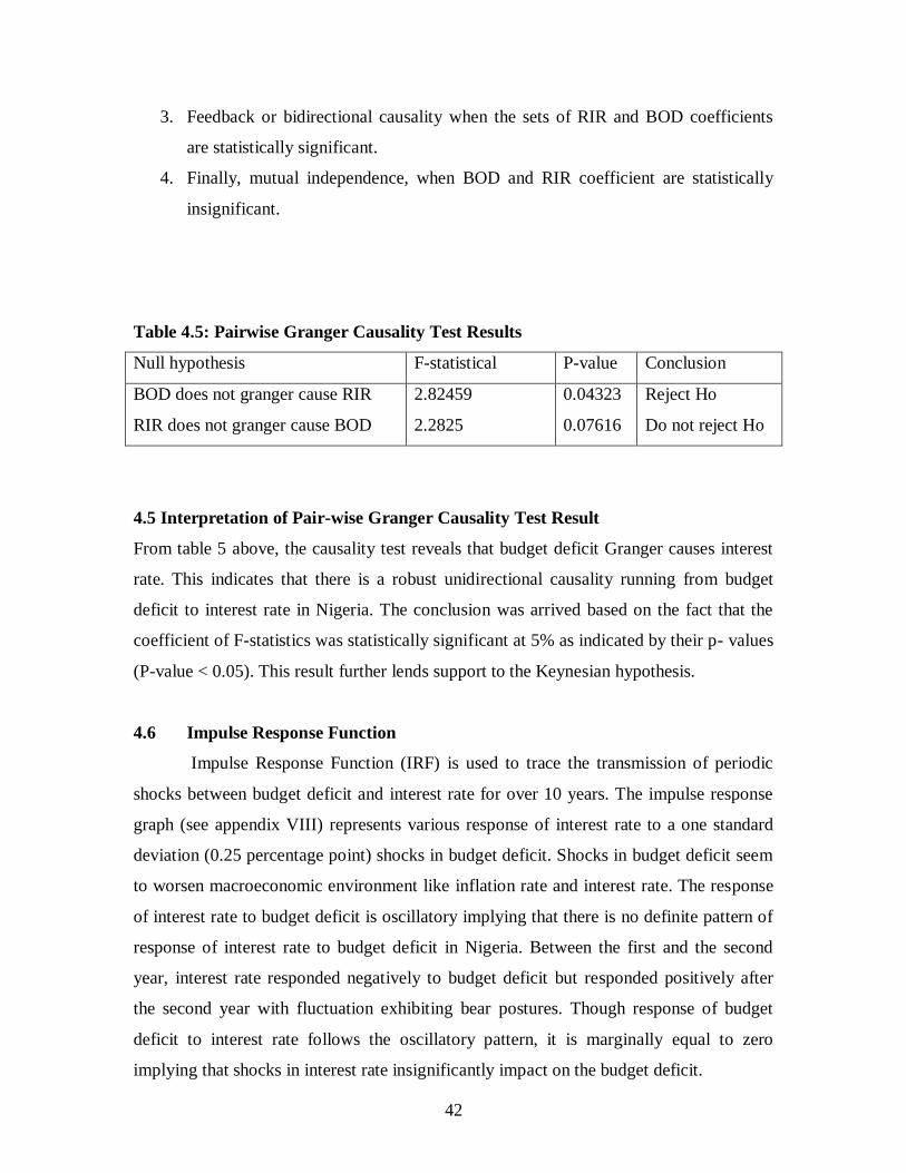
42

3. Feedback or bidirectional causality when the sets of RIR and BOD coefficients

are statistically significant.

4. Finally, mutual independence, when BOD and RIR coefficient are statistically

insignificant.

Table 4.5: Pairwise Granger Causality Test Results

Null hypothesis F-statistical P-value Conclusion

BOD does not granger cause RIR

RIR does not granger cause BOD

2.82459

2.2825

0.04323

0.07616

Reject Ho

Do not reject Ho

4.5 Interpretation of Pair-wise Granger Causality Test Result

From table 5 above, the causality test reveals that budget deficit Granger causes interest

rate. This indicates that there is a robust unidirectional causality running from budget

deficit to interest rate in Nigeria. The conclusion was arrived based on the fact that the

coefficient of F-statistics was statistically significant at 5% as indicated by their p- values

(P-value < 0.05). This result further lends support to the Keynesian hypothesis.

4.6 Impulse Response Function

Impulse Response Function (IRF) is used to trace the transmission of periodic

shocks between budget deficit and interest rate for over 10 years. The impulse response

graph (see appendix VIII) represents various response of interest rate to a one standard

deviation (0.25 percentage point) shocks in budget deficit. Shocks in budget deficit seem

to worsen macroeconomic environment like inflation rate and interest rate. The response

of interest rate to budget deficit is oscillatory implying that there is no definite pattern of

response of interest rate to budget deficit in Nigeria. Between the first and the second

year, interest rate responded negatively to budget deficit but responded positively after

the second year with fluctuation exhibiting bear postures. Though response of budget

deficit to interest rate follows the oscillatory pattern, it is marginally equal to zero

implying that shocks in interest rate insignificantly impact on the budget deficit.

43

4.7 Forecast Error Variance Decomposition

The forecast error variance between budget deficit and interest rate was examined

using Cholesky Forecast Error Variances Decomposition (FEVD) for a period of ten

years (see appendix VII). This is computed by orthogonalizing the innovations with

Cholesky decomposition. After ten periods, the budget deficit accounted for 19.3% of the

forecast error in interest rate, while money supply and inflation rate accounted for 30.8%

and 6.2% respectively accounted for the error variance in interest rate in Nigeria.

On the other hand, interest rate, money supply and inflation accounted for 4.2%,

47.9% and 13.4% respectively for the variance in budget deficit in Nigeria. This suggests

that money supply and inflation rate seem to be the driving force behind budget deficit

variance.

4.8 Test of Multicollinearity.

Multicollinearity test is used here to ascertain the violation of the assumption of

randomness of the classical linear regression model. In carrying out the test, we make use

of the correlation matrix table. The result is shown in table 6 below.

Decision Rule:

If the pair–wise or zero–order correlation coefficient between two explanatory

variables is high, say in excess of 0.8, then multicollinearity is a serious problem

(Gujarati and Sangeetha, 2007).

Tabie 4.6: Correlation Matrix. Series: ASI EXR INT INF

MOS BOD RIR INF

MOS 1.000000 -0.469125 0.101354 -0.176463

BOD -0.469125 1.000000 -0.472810 0.152142

RIR 0.101354 -0.472810 1.000000 0.338596

INF -0.176463 0.152142 0.338596 1.000000

From table 6 above, it can be seen that all the variables show no multicollinearity

since their pair-wise or zero order correlation coefficient is not up to or greater than 0.8.

44

Consequently, we conclude that there is no multicollinearity among the variables, and the

randomness of the explanatory variables is hereby met.

4.9 Test for Hetroscedasticity

The primary reason to test for hetroscedasticity after running for OLS is to detect

violation of assumption OLS:5, which is one of the assumptions needed for the usual

statistics accompanying OLS regression to be valid. The F – statistics can be used to

verify this assumption, and the hypothesis is formulated as follow:

Hypothesis

Ho: (There is no hetroscedasticity, i.e. homoscedasticity)

H1: (There is hetroscedasticity)

Decision Rule; Reject Ho if the calculated F value is greater than the tabulated F value,

otherwise accept Ho. The hetroscedasticity result is presented as;

White Heteroskedasticity Test:

F-statistic 1.064471 Probability 0.429234

Obs*R-squared 10.76422 Probability 0.376180

Following the above result, calculated F value = 1.064471 and the F probability

value = 0.429234. Therefore, since the calculated value of 1.064471 and F probability is

not significant we then accept Ho of homoscedasticity and conclude that the conditional

variances of the error terms are equal.

4.10 Normality Test

This test is to enable us determine whether the residual follow the normal

distribution as postulated by classical OLS assumption. This is tested using the Jarque-

Bera test. The hypothesis is formulated as follows:

Ho: µ = 0 (Residual follow normal distribution)

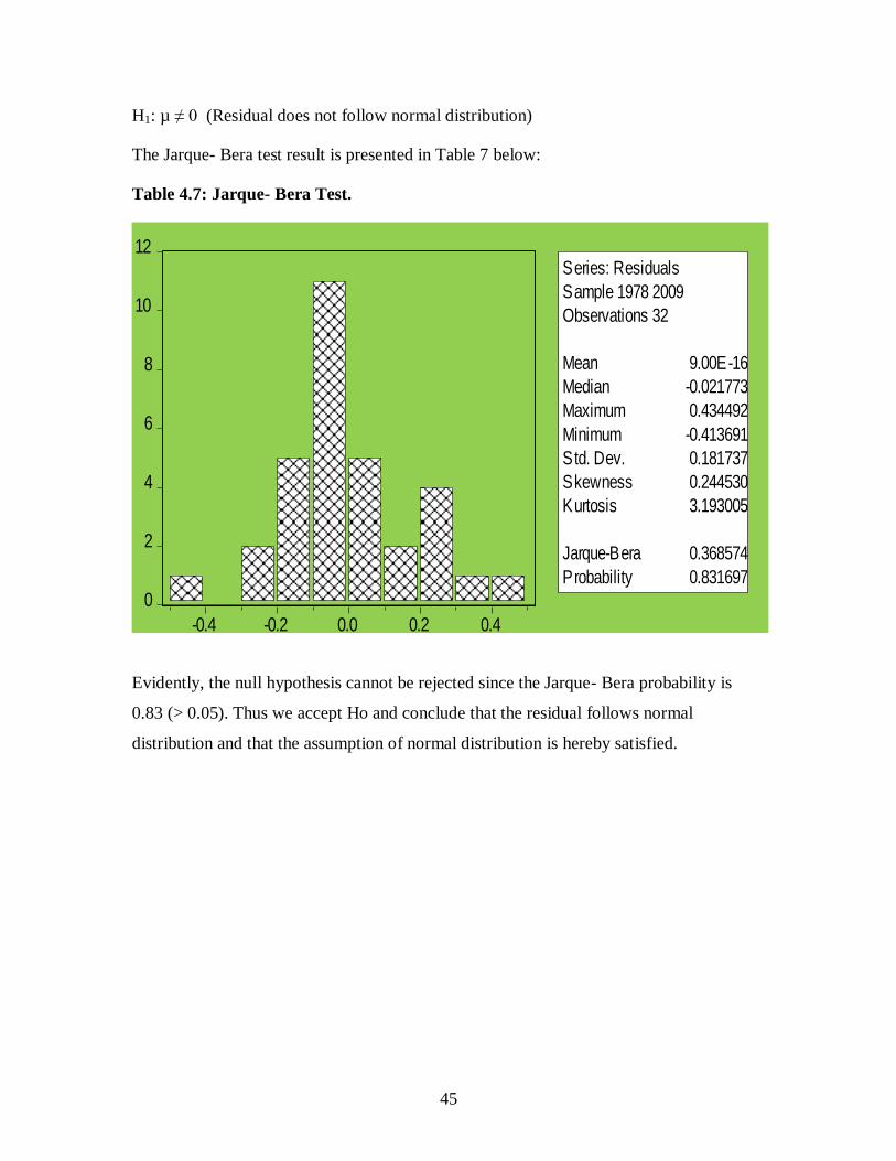
45

H1: µ ≠ 0 (Residual does not follow normal distribution)

The Jarque- Bera test result is presented in Table 7 below:

Table 4.7: Jarque- Bera Test.

0

2

4

6

8

10

12

-0.4 -0.2 0.0 0.2 0.4

Series: Residuals

Sample 1978 2009

Observations 32

Mean 9.00E-16

Median -0.021773

Maximum 0.434492

Minimum -0.413691

Std. Dev. 0.181737

Skewness 0.244530

Kurtosis 3.193005

Jarque-Bera 0.368574

Probability 0.831697

Evidently, the null hypothesis cannot be rejected since the Jarque- Bera probability is

0.83 (> 0.05). Thus we accept Ho and conclude that the residual follows normal

distribution and that the assumption of normal distribution is hereby satisfied.

46

4.11 The Graphical Trend of the Residuals of the Variables used

-1 0

-5

0

5

1 0

7 0 7 5 8 0 8 5 9 0 9 5 0 0 0 5 1 0

D(RIR) Residuals

-1 5 0 0 0 0

-1 0 0 0 0 0

-5 0 0 0 0

0

5 0 0 0 0

1 0 0 0 0 0

1 5 0 0 0 0

2 0 0 0 0 0

7 0 7 5 8 0 8 5 9 0 9 5 0 0 0 5 1 0

D(BOD) Residuals

-1 5 0 0 0 0 0

-1 0 0 0 0 0 0

-5 0 0 0 0 0

0

5 0 0 0 0 0

1 0 0 0 0 0 0

1 5 0 0 0 0 0

2 0 0 0 0 0 0

7 0 7 5 8 0 8 5 9 0 9 5 0 0 0 5 1 0

D(MOS) Residuals

-6 0

-4 0

-2 0

0

2 0

4 0

6 0

7 0 7 5 8 0 8 5 9 0 9 5 0 0 0 5 1 0

D(INF) Residuals

The residuals trend above for interest rate (RIR) maintained the interval of 5 between

1970 and 1985 but drifted away from the interval between 1986 and 1995 and thereafter

moved back to the interval. Budget deficit residuals moved within the interval of 2000

but started oscillating from 1992 to 2010. While residuals of inflation rate was oscillatory

during this period, that of money supply maintained an interval of 3000 and became

explosive after 2006.

4.12 Evaluation of the Research Questions

The research questions are basically two namely; does budget deficit interacts

with interest rate? In other words, is there any relationship between budget deficit and

47

interest rate in Nigeria? What is the direction of the relationship between budget deficit

and interest rate? Evidence from the results shows that budget deficit has both positive

and significant impact on interest rate in Nigeria. And also there is unidirectional

causality running from budget deficit to interest rate in Nigeria

48

CHAPTER FIVE

5.0 SUMMARY OF FINDINGS AND RECOMMENATIONS

This chapter is concerned with the summary of main findings drawn from the empirical

results and necessary recommendations based on research findings.

5.1 Summary of Findings

The main findings are itemized below as follows:

The ADF results show that the series are non stationary in their level form and are

integrated of order one.

Johansen co-integration test result shows evidence of co-integration implying that

there is a long run relationship between budget deficit and interest rate in Nigeria.

The VECM result shows that there is a significant positive long-run relationship

between budget deficit and interest rate suggesting that an increase in budget

deficit impacts positively on interest rate. This validates the Keynesian

Proposition.

Money supply had positive but insignificant impact on interest rate. This suggests

that a rise in interest rate will increase money supply in the country.

Inflation rate (INF) had positive but insignificant impact on interest rate contrary

to economic theory which postulates that during inflationary period, there is a

shift from investment to consumption which leads to a fall in demand for market

instrument and hence a fall in interest rate.

The causality test reveals that budget deficit Granger causes interest rate

indicating that there is a robust unidirectional causality running from budget

deficit to interest rate in Nigeria.

5.2 Recommendations

Based on the research findings, the following recommendations were made to arrest

the enumerated problems.

Since there is a long run positive impact of budget deficit on interest rate in

Nigeria, appropriate monetary- fiscal policies mix should be pursued. To achieve

this, focus should be the on the following:

49

Policy makers should focus on the right combination of appropriate internal-

external debt ratio, the ways and means and bond to finance budget deficit in the

country with close monitoring of inflation.

Since the causality test revealed that there is a robust unidirectional causality

running from budget deficit to interest rate in Nigeria, deficit could be reduced

through higher revenue and faster growth because high and seemingly intractable

budget deficits suggest little scope for fiscal stimulus.

Restrictive monetary, fiscal, and exchange rate policies should be maintained in

order to fight highly pervasive and persistent increase in the general price level

and increasing interest rate.

Inflation-adjusted interest rate policy should be pursued in order to reduce the cost

of servicing debt and the budget deficit.

50

REFERENCES

Afonso, A. and Strauch R. (2004) Fiscal Policy Events and Interest Rate Swap spreads:

Evidence from the E.U. ECB working paper 303, February

.

Aisen, A. and Hauner D, (2008) Budget Deficits and Interest Rates. A Fresh Perspective.

IMF Working Paper. WP/08/42.

Anyanwu, J.C.(1998) Do Fiscal Deficits Produce High Interest Rates: The Case of

Nigeria, Ghana and the Gambia, CBN Economic and Financial Preview, Vol. 36,

No.1.

Barro R (1974), Are Government Bonds Net Wealth? Journal of Political Economy,

82,6,Nov/Dec, PP:1097-1117.

Barro R (1987), Government Spending, Interest Rates, Prices, and Budget Deficits in the

United Kingdom, 1701-1918, Journal of Monetary Economics, 20, No.2, September,

PP.221-47.

Barro, R.J (1989b) “ The Ricardian Approach to Budget Deficits” Journal of Economic

Perspectives, Vol.3 (2), P.37- 54.

Beard, T.R and Mcmillin, W.D.(1991), The Impact of Budgets in the Interwar Period

Journal of Macroeconomics, 13,No.2, Spring, PP.239-66.

Berheim, B.D., (1989), “A Neoclassical Perspective on Budget Deficits,” Journal of

economic Perspective 3,55-72.

Berheim B.D. (1987) IN: William, E and Schmidt Hebbel, K Editors. Public Sector

Deficits, and Macroeconomic Performance, Publisher for the Word Bank, Oxford

University Press

Blinder, A.S. and Solow, R.M. (1973) “Does Fiscal Policy Matter?”, Journal of Public

Economics Vol. 2, P.318-37

Blinder, A.S and Solow, R.M (1976) “ Does Fiscal Policy Still Matter?”, Journal of

Public Economics Vol.5, P.501-10.

Bovenberg, L.A.(1998), Long – Term Interest Rates in the United States: An Empirical

Analysis, IMF Staff Papers, 35, No.2, June, PP.382-90.

Bhalla, S. (1995) This Time, It Is Already Different: A Personal Perspective, Deutshe

Bank, December 7.

51

Cheug, B.S. (1998), The Causality Between Budget Deficits and Interests Rates in Japan:

An Application of Time Services Analysis, Applied Economic Letters, 5, No.7, July

PP.419-22.

Corbo and Schmidt-Hebbel, K. (1991) IN, William, E.and Schmidt Hebbel K. Editor

Public Deficits and Macroeconomic Performance. Published For The Word Bank.,

Oxford University Press.

Chimobi, O.P. and Igwe, O.L. (2010) Budget Deficit, Money Supply and Inflation. Euro

Journal’s,INC.

Cohen, D. and Garner, O. (1991). The impact of Forests of Budget Deficits on Interest

Rates in The United States and Other G-7 Countries, Federal Reserve Board.

Codogno, L; Favero, C. and Missale, A. (2003) Yield Spread on EMU Government

Boards, Economic Policy, October, PP 505-532.

Darrat, A.F. (1990), Structural Federal Deficits and Interest Rates: Some Causality and

Cointeggration Tests, Southern Economic Journal,56, No3,January PP.752-59.

Dua, P. (1993), Interest Rates, Government Purchases and budget Deficit: A forward-

looking model, Public Financial Quarterly

Dai, Q. and Philippians, T. (2004), Government Deficits and Interest Rates: A. No-

Arbitrage Structural VAR Approached, New York University First Draft, March 14.

Edward, S. and kahn, M.S. (1985) “Interest Determination in Developing Countries: 32,

377-403.

Easterly, W.E and Schmidt-Hebbel K.(1993), “Fiscal Deficits and macroeconomic

Performance in Developing Countries” Word Bank Research Observer 8, 211-37.

Evans, P. (1987). Do Budget Deficits Raise Nominal Interest Rates?, Journal of

Monetary Economics 20, No.2 September, PP.281-300.

Gale, W.G. and Orszag, P.R (2003). The Economic Effects of Long-Term Fiscal

Discipline. The Urban-Brookings Tax policy Center Discussion Paper 8, April.

Gale, W.G and Orszag, P.R. (2003), “Economic Effects of Sustained Fiscal Deficits”

National Tax Journal 56, 463-485.

Gujarati, N.D. (2003) Fiscal Policy Events and Interest Rate Swap Spreads: Evidence

From the Eu. ECB Working Paper 303, February.

Hayashi (1985) IN; William, E and O. Schmidt-Hebbel, K. Public Sector Deficits and

Macroeconomic Performance Published for the Word Bank. Oxford University Press.

Haque and Montiel IN; William, E and Schmidt Hebbel, K. Public deficits and

Macroeconomic Performance. Published for the Word Bank, Oxford University Press

52

.

Haliassos, M and Tobin, J. (1990) “The Macroeconomics of Government Finance”, in

Friedman and Hahn, Editors, Hand Book of Monetary Economics Volume II.

Amsterdam: North-Holland.

Heppke-Falk, K. and Hufner, F. (2004), Expected Budget Deficits and Interest Rate Swap

Spreads Discussion paper series 1: Studies of the Economic Research Centre. No. 40.

Johansen, S.. (1991) Estimation and Hypothesis Testing of Cointegration Vectors in

Gaussian Vector Autoregressive Models Econometrics, 59, No6 Nov., PP. 1551- 80

Johansen, S. (1995), Likelihood-Based Interference in Cointegrated Vector

Autoregressive Models, Oxford University. Press, Oxford.

Johansen, S. (1988), Statistical Analysis of Cointgration Vectors, Journal of Economic

Dynamics and control, 12, No. 2/3 June/ September..,

Leiderman and Blejer (1988) IN; William, E and Schmidt-Hebbel, K. Editor Public

Sector Deficits and Macroeconomic Performance Published for the World Bank,

Oxford University Press.

Laumas, G.S (1989), Anticipated Federal Budget Deficits, Monetary Policy and the Rate

of Interest Southern Economic Journal, 56, No.2 October., PP.375.82.

Lal, D; Blinde, S and Vasudevan, D. (2002). Financial Exuberence: Savings Deposits,

Fiscal Deficits and Interest of Rates in India, Working paper No.821, Department of

Economics, University of California, Cos Angles.

Laubauch, T. (2003) New Evidence on the Interest Rate Effect Of budget Deficits and

Debt, Board of Governors of the Federal Reserve System.

Labonte, M. (2005). Do Budget Deficits Publish up Interest Rates and Is this the Relevant

Question? CRS Report for Congress.

Makin, J. H. (1983) “Real Interest Money Surprises, Anticipated Inflation and fiscal

deficit”. Review of Economic and Statistics Vol.65, P.374-84

Obi, B. and Nurudeen, A. (2008). “Effect, of Fiscal Deficits and Government Debt:

Journal of Applied Quantitative Methods. Vol.4 No.3.

Seater, J.J (1993) “Ricardian Equivalence” Journal of Economic Literature, Vol. 31 (1),

P. 142-90.

Seater J.J. (1993) IN; William E and Schimidt-Hebbel, K. Public Sector Deficits and

Microeconomic Performance Published for the World Bank, Oxford University Press.

Tobin, J.. and Buiter, W.H (1976) “ Long-Run Effect of Fiscal and Monetary Policy” In

Stein, editor, Monetarism, Amstredan: North Holland.

53

Ussher, L.J. (1998) Do Budget Deficits Raise Interest Rates? Transformational Growth

and Full Employment, Working Paper, No. 3 New School for Research.

Vemvoukas, G.A. Gargalas, V.N. and Lehman, H. H. (2008) Testing Keynesian

Proposition and Ricardiance Equivalence: More Evidence on the Debate Journal of

Business and Economic Research.

Watehel; P. and Young, J. (1987) Deficit Announcements and Interest Rates American

Economic Review 77, P.P1007-1012.

World Bank Policy Research Bulletin, Vol.4 No3, May-July 1993.

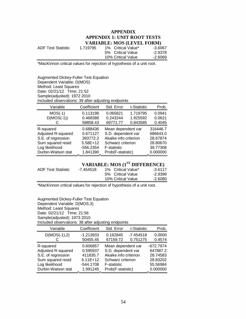
54

APPENDIX

APPENDIX 1: UNIT ROOT TESTS

VARIABLE: MOS (LEVEL FORM) ADF Test Statistic 1.719795 1% Critical Value* -3.6067

5% Critical Value -2.9378 10% Critical Value -2.6069

*MacKinnon critical values for rejection of hypothesis of a unit root.

Augmented Dickey-Fuller Test Equation Dependent Variable: D(MOS) Method: Least Squares Date: 02/21/12 Time: 21:52 Sample(adjusted): 1972 2010 Included observations: 39 after adjusting endpoints

Variable Coefficient Std. Error t-Statistic Prob.

MOS(-1) 0.113198 0.065821 1.719795 0.0941 D(MOS(-1)) 0.468388 0.243244 1.925592 0.0621

C 58858.43 69771.77 0.843585 0.4045

R-squared 0.688436 Mean dependent var 316446.7 Adjusted R-squared 0.671127 S.D. dependent var 686643.0 S.E. of regression 393772.2 Akaike info criterion 28.67874 Sum squared resid 5.58E+12 Schwarz criterion 28.80670 Log likelihood -556.2354 F-statistic 39.77308 Durbin-Watson stat 1.841390 Prob(F-statistic) 0.000000

VARIABLE: MOS (1ST

DIFFERENCE) ADF Test Statistic -7.454518 1% Critical Value* -3.6117

5% Critical Value -2.9399 10% Critical Value -2.6080

*MacKinnon critical values for rejection of hypothesis of a unit root.

Augmented Dickey-Fuller Test Equation Dependent Variable: D(MOS,3) Method: Least Squares Date: 02/21/12 Time: 21:56 Sample(adjusted): 1973 2010 Included observations: 38 after adjusting endpoints

Variable Coefficient Std. Error t-Statistic Prob.

D(MOS(-1),2) -1.213933 0.162845 -7.454518 0.0000 C 50455.45 67159.72 0.751275 0.4574

R-squared 0.606857 Mean dependent var -672.7974 Adjusted R-squared 0.595937 S.D. dependent var 647887.2 S.E. of regression 411835.7 Akaike info criterion 28.74583 Sum squared resid 6.11E+12 Schwarz criterion 28.83202 Log likelihood -544.1708 F-statistic 55.56984 Durbin-Watson stat 1.991245 Prob(F-statistic) 0.000000

55

VARIABLE: BOD (LEVEL FORM)

ADF Test Statistic -1.568064 1% Critical Value* -3.6067

5% Critical Value -2.9378 10% Critical Value -2.6069

*MacKinnon critical values for rejection of hypothesis of a unit root.

Augmented Dickey-Fuller Test Equation Dependent Variable: D(BOD) Method: Least Squares Date: 02/21/12 Time: 21:57 Sample(adjusted): 1972 2010 Included observations: 39 after adjusting endpoints

Variable Coefficient Std. Error t-Statistic Prob.

BOD(-1) -0.187707 0.119706 -1.568064 0.1256 D(BOD(-1)) -0.053997 0.175724 -0.307280 0.7604

C -16925.32 11557.30 -1.464470 0.1517

R-squared 0.083784 Mean dependent var -5944.795 Adjusted R-squared 0.032883 S.D. dependent var 59824.57 S.E. of regression 58832.75 Akaike info criterion 24.87659 Sum squared resid 1.25E+11 Schwarz criterion 25.00455 Log likelihood -482.0935 F-statistic 1.646018 Durbin-Watson stat 1.932834 Prob(F-statistic) 0.206997

VARIABLE: BOD (1ST

DIFFERENCE)

ADF Test Statistic -5.877872 1% Critical Value* -3.6117

5% Critical Value -2.9399 10% Critical Value -2.6080

*MacKinnon critical values for rejection of hypothesis of a unit root.

Augmented Dickey-Fuller Test Equation Dependent Variable: D(BOD,2) Method: Least Squares Date: 02/21/12 Time: 22:00 Sample(adjusted): 1973 2010 Included observations: 38 after adjusting endpoints

Variable Coefficient Std. Error t-Statistic Prob.

D(BOD(-1)) -1.562676 0.265857 -5.877872 0.0000 D(BOD(-1),2) 0.340160 0.172846 1.967992 0.0570

C -7310.385 9515.737 -0.768242 0.4475

R-squared 0.603337 Mean dependent var -2521.613 Adjusted R-squared 0.580670 S.D. dependent var 90354.16 S.E. of regression 58509.46 Akaike info criterion 24.86742 Sum squared resid 1.20E+11 Schwarz criterion 24.99670 Log likelihood -469.4810 F-statistic 26.61801 Durbin-Watson stat 1.891468 Prob(F-statistic) 0.000000

56

VARIABLE: RIR (LEVEL FORM)

ADF Test Statistic -1.507153 1% Critical Value* -3.6067

5% Critical Value -2.9378 10% Critical Value -2.6069

*MacKinnon critical values for rejection of hypothesis of a unit root.

Augmented Dickey-Fuller Test Equation Dependent Variable: D(RIR) Method: Least Squares Date: 02/21/12 Time: 22:01 Sample(adjusted): 1972 2010 Included observations: 39 after adjusting endpoints

Variable Coefficient Std. Error t-Statistic Prob.

RIR(-1) -0.136263 0.090411 -1.507153 0.1405 D(RIR(-1)) -0.374941 0.151107 -2.481288 0.0179

C 2.245996 1.451110 1.547778 0.1304

R-squared 0.238653 Mean dependent var 0.169744 Adjusted R-squared 0.196355 S.D. dependent var 3.987689 S.E. of regression 3.574813 Akaike info criterion 5.459506 Sum squared resid 460.0543 Schwarz criterion 5.587472 Log likelihood -103.4604 F-statistic 5.642293 Durbin-Watson stat 2.107233 Prob(F-statistic) 0.007387

VARIABLE: RIR (1ST

DIFFERENCE)

ADF Test Statistic -5.923274 1% Critical Value* -3.6117

5% Critical Value -2.9399 10% Critical Value -2.6080

*MacKinnon critical values for rejection of hypothesis of a unit root.

Augmented Dickey-Fuller Test Equation Dependent Variable: D(RIR,2) Method: Least Squares Date: 02/21/12 Time: 22:03 Sample(adjusted): 1973 2010 Included observations: 38 after adjusting endpoints

Variable Coefficient Std. Error t-Statistic Prob.

D(RIR(-1)) -1.681632 0.283903 -5.923274 0.0000 D(RIR(-1),2) 0.170765 0.168118 1.015747 0.3167

C 0.294645 0.600264 0.490859 0.6266

R-squared 0.726347 Mean dependent var 0.017105 Adjusted R-squared 0.710709 S.D. dependent var 6.849452 S.E. of regression 3.684028 Akaike info criterion 5.521547 Sum squared resid 475.0223 Schwarz criterion 5.650831 Log likelihood -101.9094 F-statistic 46.44955 Durbin-Watson stat 1.909569 Prob(F-statistic) 0.000000

57

VARIABLE: INF (LEVEL FORM)

ADF Test Statistic -1.765936 1% Critical Value* -3.6228

5% Critical Value -2.9446 10% Critical Value -2.6105

*MacKinnon critical values for rejection of hypothesis of a unit root.

Augmented Dickey-Fuller Test Equation Dependent Variable: D(INF) Method: Least Squares Date: 02/21/12 Time: 22:06 Sample(adjusted): 1975 2010 Included observations: 36 after adjusting endpoints

Variable Coefficient Std. Error t-Statistic Prob.

INF(-1) -0.416069 0.235608 -1.765936 0.0876 D(INF(-1)) 0.074337 0.221506 0.335597 0.7395 D(INF(-2)) -0.200996 0.207565 -0.968356 0.3406 D(INF(-3)) -0.041645 0.180403 -0.230843 0.8190 D(INF(-4)) -0.315754 0.170363 -1.853420 0.0737

C 8.965302 5.637874 1.590192 0.1223

R-squared 0.352848 Mean dependent var -0.053611 Adjusted R-squared 0.244989 S.D. dependent var 18.25427 S.E. of regression 15.86138 Akaike info criterion 8.516664 Sum squared resid 7547.505 Schwarz criterion 8.780584 Log likelihood -147.2999 F-statistic 3.271391 Durbin-Watson stat 1.843480 Prob(F-statistic) 0.017831

VARIABLE: INF (1ST

DIFFERENCE)

ADF Test Statistic -5.880404 1% Critical Value* -3.6117

5% Critical Value -2.9399 10% Critical Value -2.6080

*MacKinnon critical values for rejection of hypothesis of a unit root.

Augmented Dickey-Fuller Test Equation Dependent Variable: D(INF,2) Method: Least Squares Date: 02/21/12 Time: 22:08 Sample(adjusted): 1973 2010 Included observations: 38 after adjusting endpoints

Variable Coefficient Std. Error t-Statistic Prob.

D(INF(-1)) -1.398720 0.237861 -5.880404 0.0000 D(INF(-1),2) 0.289054 0.161463 1.790213 0.0821

C 0.190205 2.837419 0.067034 0.9469

R-squared 0.581959 Mean dependent var -0.225263 Adjusted R-squared 0.558071 S.D. dependent var 26.30172 S.E. of regression 17.48478 Akaike info criterion 8.636196 Sum squared resid 10700.12 Schwarz criterion 8.765479 Log likelihood -161.0877 F-statistic 24.36196 Durbin-Watson stat 2.073732 Prob(F-statistic) 0.000000

58

APPENDIX II

JOHANSEN CO-INTEGRATION PROCEDURE.VARIABLE:RIR BOD MOS INF

Date: 02/21/12 Time: 22:12 Sample: 1970 2010 Included observations: 38

Test assumption:

Linear deterministic trend in the

data

Series: RIR BOD MOS INF Lags interval: 1 to 2

Likelihood 5 Percent 1 Percent Hypothesized Eigenvalue Ratio Critical Value Critical Value No. of CE(s)

0.592983 48.35599 47.21 54.46 None * 0.250614 14.19782 29.68 35.65 At most 1 0.078428 3.234779 15.41 20.04 At most 2 0.003446 0.131155 3.76 6.65 At most 3

*(**) denotes rejection of the hypothesis at

5%(1%) significance

level

L.R. test indicates 1

cointegrating equation(s) at

5% significance

level

Unnormalized Cointegrating Coefficients:

RIR BOD MOS INF -0.033882 -1.94E-06 1.92E-07 0.018511 0.009235 6.62E-07 5.46E-07 -0.004675 0.027776 2.51E-06 2.27E-07 0.000893 0.009762 -2.84E-06 -5.52E-07 0.000332

Normalized

Cointegrating Coefficients: 1 Cointegrating Equation(s)

RIR BOD MOS INF C 1.000000 5.73E-05 -5.66E-06 -0.546349 6.268000

(1.4E-05) (3.4E-06) (0.06760)

Log likelihood -1239.804

Normalized

59

Cointegrating Coefficients: 2 Cointegrating Equation(s)

RIR BOD MOS INF C 1.000000 0.000000 -0.000265 -0.706413 307.4535

(0.00189) (2.49738) 0.000000 1.000000 4.517953 2791.972 -5253526.

(32.7267) (43357.1)

Log likelihood -1234.323

Normalized

Cointegrating Coefficients: 3 Cointegrating Equation(s)

RIR BOD MOS INF C 1.000000 0.000000 0.000000 -1.661083 19.39563

(2.97745) 0.000000 1.000000 0.000000 19087.87 -336476.9

(49001.7) 0.000000 0.000000 1.000000 -3606.922 -1088336.

(37060.9)

Log likelihood -1232.771

60

APPENDIX III

VECM TESTS Date: 02/21/12 Time: 22:18 Sample(adjusted): 1974 2010 Included observations: 37 after adjusting endpoints Standard errors & t-statistics in parentheses

Cointegrating Eq: CointEq1

D(RIR(-1)) 1.000000

D(BOD(-1)) 0.48570 (0.13392) (3.62681)

D(MOS(-1)) 7.20E-05 (0.00019) (0.38053)

D(INF(-1)) 2.371175 (6.38009) (0.37165)

C -23.85451

Error Correction: D(RIR,2) D(BOD,2) D(MOS,2) D(INF,2)

CointEq1 -0.370534 1234.346 -3587.637 -0.170534 (0.13392) (381.232) (2749.88) (0.13392) (-2.76681) (3.23778) (-1.30465) (-0.76681)

D(RIR(-1),2) -1.127498 2485.080 13632.58 0.241357 (0.16447) (2907.22) (20970.2) (1.02126) (-6.85519) (0.85480) (0.65009) (0.23633)

D(RIR(-2),2) -0.531250 2357.203 13269.94 0.757106 (0.14519) (2566.43) (18512.0) (0.90155) (-3.65891) (0.91848) (0.71683) (0.83978)

D(BOD(-1),2) -2.89E-05 -0.186735 -2.190727 -0.000205 (1.2E-05) (0.21325) (1.53824) (7.5E-05) (-2.39174) (-0.87564) (-1.42418) (-2.73956)

D(BOD(-2),2) -9.30E-06 -0.135113 -0.561572 -0.000124 (1.1E-05) (0.19347) (1.39550) (6.8E-05) (-0.84974) (-0.69838) (-0.40242) (-1.82186)

D(MOS(-1),2) 7.89E-07 -0.099615 0.024369 2.45E-05 (2.0E-06) (0.03581) (0.25829) (1.3E-05) (0.38964) (-2.78196) (0.09435) (1.95155)

D(MOS(-2),2) 1.37E-06 -0.237651 0.375296 5.44E-05 (3.8E-06) (0.06794) (0.49010) (2.4E-05) (0.35520) (-3.49769) (0.76576) (2.27815)

D(INF(-1),2) 0.110448 -2248.089 5885.434 0.039660 (0.04296) (759.318) (5477.07) (0.26674) (2.57108) (-2.96067) (1.07456) (0.14869)

D(INF(-2),2) 0.062916 -1640.040 1892.670 -0.031648

61

(0.03658) (646.577) (4663.85) (0.22713) (1.71998) (-2.53649) (0.40582) (-0.13933)

C -0.280021 23087.47 5971.928 -6.085101 (0.71010) (12551.7) (90536.9) (4.40921) (-0.39434) (1.83940) (0.06596) (-1.38009)

R-squared 0.808140 0.655510 0.153665 0.495257 Adj. R-squared 0.744187 0.540680 -0.128447 0.327009 Sum sq. resids 333.0412 1.04E+11 5.41E+12 12840.48 S.E. equation 3.512102 62079.62 447789.0 21.80764 F-statistic 12.63640 5.708520 0.544694 2.943614 Log likelihood -93.15167 -455.0101 -528.1186 -160.7154 Akaike AIC 5.575766 25.13568 29.08749 9.227857 Schwarz SC 6.011149 25.57107 29.52287 9.663241 Mean dependent 0.017568 -2602.070 42561.57 0.108108 S.D. dependent 6.943932 91599.10 421534.2 26.58300

Determinant Residual Covariance

7.59E+23

Log Likelihood -1227.240 Akaike Information Criteria 68.71570 Schwarz Criteria 70.63139

APPENDIX IV

GRANGER CAUSALITY TEST Pairwise Granger Causality Tests Date: 02/24/12 Time: 05:05 Sample: 1970 2010 Lags: 8

Null Hypothesis: Obs F-Statistic Probability

BOD does not Granger Cause RIR 33 2.82459 0.04323 RIR does not Granger Cause BOD 2.28254 0.07616

62

APPENDIX V: HETEROSKEDASTICITY TEST

F-statistic 1.064471 Probability 0.429234 Obs*R-squared 10.76422 Probability 0.376180

Test Equation: Dependent Variable: RESID^2 Method: Least Squares Date: 02/12/12 Time: 17:11 Sample: 1978 2009 Included observations: 32

Variable Coefficient Std. Error t-Statistic Prob.

C -0.173499 0.148521 -1.168179 0.2558 RIR(-1) 0.024586 0.012531 1.962049 0.0631

RIR(-1)^2 -0.000655 0.000309 -2.123574 0.0458 BOD -0.033482 0.023901 -1.400887 0.1759

BOD^2 0.005080 0.002535 2.004293 0.0581 RIR 0.018104 0.015429 1.173350 0.2538

RIR^2 -0.005988 0.003706 -1.615989 0.1210 INF 0.001557 0.001876 0.829860 0.4160

INF^2 -2.40E-05 2.51E-05 -0.956026 0.3499 MOS 0.032842 0.058110 0.565167 0.5779

MOS^2 -0.014629 0.016515 -0.885832 0.3857

R-squared 0.336382 Mean dependent var 0.031996 Adjusted R-squared 0.020373 S.D. dependent var 0.048141 S.E. of regression 0.047648 Akaike info criterion -2.983670 Sum squared resid 0.047677 Schwarz criterion -2.479823 Log likelihood 58.73872 F-statistic 1.064471 Durbin-Watson stat 2.135722 Prob(F-statistic) 0.429234

63

APPENDIX VI: NORMALITY TEST

0

2

4

6

8

10

12

-0.4 -0.2 0.0 0.2 0.4

Series: Residuals

Sample 1978 2009

Observations 32

Mean 9.00E-16

Median -0.021773

Maximum 0.434492

Minimum -0.413691

Std. Dev. 0.181737

Skewness 0.244530

Kurtosis 3.193005

Jarque-Bera 0.368574

Probability 0.831697

APPENDIX VII

VARIANCE DECOMPOSITION RESULT Variance

Decomposition of D(RIR

):

Period

S.E. D(RIR) D(BOD) D(MOS) D(INF)

1 3.000185 100.0000 0.000000 0.000000 0.000000 2 3.411882 82.75339 4.343916 1.277771 11.62492 3 4.207564 74.37237 11.51864 1.322690 12.78630 4 4.656671 74.15332 9.764997 4.889504 11.19218 5 6.074061 43.93220 15.61404 33.87504 6.578719 6 6.254657 45.37284 16.03980 32.26976 6.317597 7 6.738328 40.67613 20.32685 33.02322 5.973793 8 6.820836 41.13766 20.36266 32.38612 6.113562 9 7.015791 41.68726 20.38419 32.14612 5.782427

10 7.228592 43.62989 19.32457 30.84827 6.197273

Variance

Decomposition of D(BO

64

D): Period

S.E. D(RIR) D(BOD) D(MOS) D(INF)

1 53031.03 0.365596 99.63440 0.000000 0.000000 2 55077.14 2.044713 92.51671 1.101525 4.337053 3 81836.90 2.444848 51.31215 40.27460 5.968402 4 110784.6 3.082550 49.26143 35.81783 11.83820 5 112282.4 3.794898 48.98677 35.42678 11.79155 6 123876.9 3.120582 51.26351 35.83867 9.777244 7 126553.0 3.007673 53.19137 34.42095 9.380013 8 127792.5 3.503751 52.54012 34.75718 9.198947 9 133123.0 4.240006 48.56955 36.10943 11.08102

10 136223.1 4.260363 47.87688 34.48536 13.37740

Variance

Decomposition of D(MO

S):

Period

S.E. D(RIR) D(BOD) D(MOS) D(INF)

1 382520.3 0.038160 27.97427 71.98757 0.000000 2 493158.3 1.069851 27.55373 70.56951 0.806910 3 649162.7 1.388638 30.72661 65.35451 2.530240 4 703860.8 1.829426 31.13519 62.19024 4.845152 5 723314.9 2.300804 30.98563 60.60188 6.111691 6 729395.2 2.262830 30.97621 60.72142 6.039541 7 754971.2 2.144043 30.70007 61.51815 5.637739 8 830341.5 1.887384 30.15593 63.24954 4.707150 9 911685.2 1.851868 30.58399 62.99515 4.568992

10 977526.0 2.105065 31.05504 61.50962 5.330273

Variance

Decomposition of D(INF

):

Period

S.E. D(RIR) D(BOD) D(MOS) D(INF)

1 18.62901 10.20379 4.240053 3.270384 82.28577 2 19.16708 10.27847 6.472147 3.502398 79.74699 3 23.55990 7.571648 22.99585 16.64324 52.78926 4 26.90209 6.383388 17.69536 35.02809 40.89317 5 28.89585 5.664646 15.42167 42.07454 36.83915 6 34.41792 5.330203 15.92646 47.73515 31.00818 7 36.26759 6.216038 14.40868 44.33439 35.04089 8 37.46722 6.111859 15.53423 42.30154 36.05237 9 38.14763 5.896515 17.84441 41.20002 35.05906

10 38.59530 5.776862 19.20450 40.72219 34.29645

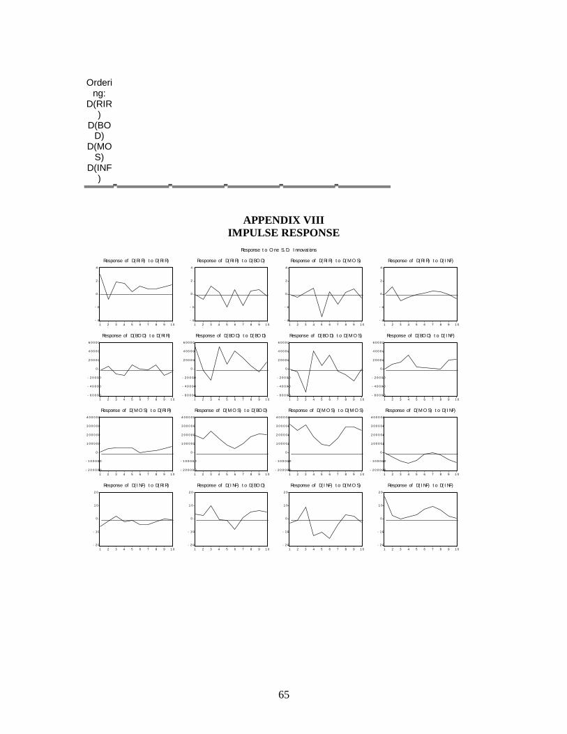
65

Orderi

ng: D(RIR

) D(BO

D) D(MO

S) D(INF

)

APPENDIX VIII

IMPULSE RESPONSE

- 4

- 2

0

2

4

1 2 3 4 5 6 7 8 9 1 0

Response of D(RI R) t o D( RI R)

- 4

- 2

0

2

4

1 2 3 4 5 6 7 8 9 1 0

Response of D(RI R) t o D( BO D)

- 4

- 2

0

2

4

1 2 3 4 5 6 7 8 9 1 0

Response of D(RI R) t o D( MO S)

- 4

- 2

0

2

4

1 2 3 4 5 6 7 8 9 1 0

Response of D(RI R) t o D( I NF)

- 6 0 0 0 0

- 4 0 0 0 0

- 2 0 0 0 0

0

2 0 0 0 0

4 0 0 0 0

6 0 0 0 0

1 2 3 4 5 6 7 8 9 1 0

Response of D(BO D) t o D( RI R)

- 6 0 0 0 0

- 4 0 0 0 0

- 2 0 0 0 0

0

2 0 0 0 0

4 0 0 0 0

6 0 0 0 0

1 2 3 4 5 6 7 8 9 1 0

Response of D(BO D) t o D( BO D)

- 6 0 0 0 0

- 4 0 0 0 0

- 2 0 0 0 0

0

2 0 0 0 0

4 0 0 0 0

6 0 0 0 0

1 2 3 4 5 6 7 8 9 1 0

Response of D(BO D) t o D( MO S)

- 6 0 0 0 0

- 4 0 0 0 0

- 2 0 0 0 0

0

2 0 0 0 0

4 0 0 0 0

6 0 0 0 0

1 2 3 4 5 6 7 8 9 1 0

Response of D(BO D) t o D( I NF)

- 2 0 0 0 0 0

- 1 0 0 0 0 0

0

1 0 0 0 0 0

2 0 0 0 0 0

3 0 0 0 0 0

4 0 0 0 0 0

1 2 3 4 5 6 7 8 9 1 0

Response of D(M O S) t o D(RI R)

- 2 0 0 0 0 0

- 1 0 0 0 0 0

0

1 0 0 0 0 0

2 0 0 0 0 0

3 0 0 0 0 0

4 0 0 0 0 0

1 2 3 4 5 6 7 8 9 1 0

Response of D(M O S) t o D(BO D)

- 2 0 0 0 0 0

- 1 0 0 0 0 0

0

1 0 0 0 0 0

2 0 0 0 0 0

3 0 0 0 0 0

4 0 0 0 0 0

1 2 3 4 5 6 7 8 9 1 0

Response of D(M O S) t o D(M O S)

- 2 0 0 0 0 0

- 1 0 0 0 0 0

0

1 0 0 0 0 0

2 0 0 0 0 0

3 0 0 0 0 0

4 0 0 0 0 0

1 2 3 4 5 6 7 8 9 1 0

Response of D(M O S) t o D( I NF)

- 2 0

- 1 0

0

1 0

2 0

1 2 3 4 5 6 7 8 9 1 0

Response of D( I NF) t o D( RI R)

- 2 0

- 1 0

0

1 0

2 0

1 2 3 4 5 6 7 8 9 1 0

Response of D( I NF) t o D( BO D)

- 2 0

- 1 0

0

1 0

2 0

1 2 3 4 5 6 7 8 9 1 0

Response of D( I NF) t o D( MO S)

- 2 0

- 1 0

0

1 0

2 0

1 2 3 4 5 6 7 8 9 1 0

Response of D( I NF) t o D( I NF)

Response t o O ne S. D. I nnovat ions