uk climate projections science report: climate change

106

UK Climate Projections science report: Climate change projections — Chapter 4

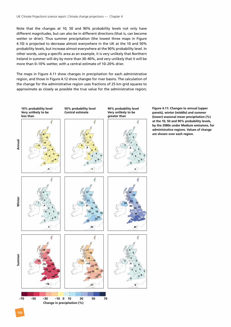
Note that the changes at 10, 50 and 90% probability levels not only have different magnitudes, but can also be in different directions (that is, can become wetter or drier). Thus summer precipitation (the lowest three maps in Figure 4.10) is projected to decrease almost everywhere in the UK at the 10 and 50% probability levels, but increase almost everywhere at the 90% probability level. In other words, using a specific area as an example, it is very unlikely that Northern Ireland in summer will dry by more than 30–40%, and very unlikely that it will be more than 0–10% wetter, with a central estimate of 10–20% drier.

The maps in Figure 4.11 show changes in precipitation for each administrative region, and those in Figure 4.12 show changes for river basins. The calculation of the change for the administrative region uses fractions of 25 km grid squares to approximate as closely as possible the true value for the administrative region;

Figure 4.11: Changes to annual (upper panels), winter (middle) and summer (lower) seasonal mean precipitation (%) at the 10, 50 and 90% probability levels, by the 2080s under Medium emissions, for administrative regions. Values of change are shown over each region.

Change in precipitation (%)–70 –50 –30 –10 0 10 30 50 70

An

nu

alW

inte

rSu

mm

er

10% probability levelVery unlikely to be less than

50% probability levelCentral estimate

90% probability levelVery unlikely to be greater than

–4

–4

–4

–4–4

–4

–7–7

–6

–6

–5

–5

–5

–5

–8

–8

00

00

00

00

00

00

0

00

–1

66

6

66

66

66

7

7

3 5

5

4

2

4

4

4

1

11

2

2

33

23

3

3

3

3

5

5

–32–32

–28–33

–36

–39

–43–43

–43–43

–49

–55

–48–47

–44–42

–16

–16–18

–22–22

–22

–19

–19–21

–23

–27

–24

–20–20

–11

–15

40

0

00

00

3

55

55

66 6

8

22

19

19

1818

14

14

11

11

17

21

21

20

16

17

3425

42

32

3249

24

42

34

3841

43

4450

54

47

107


these are the values given in Table 4.5. The User Interface plots the same colour for the whole administrative region, of course, but the resolution in this case is that of the 25 km squares. Hence some small parts of administrative regions will appear from the User Interface map to be plotted in the wrong administrative region, but the value calculated, and shown on the region, is correct. The same comment applies also to river basins in Figure 4.12.

Figure 4.13 shows changes to seasonal mean precipitation over marine regions. Winter-mean precipitation at the 50% probability level by the 2080s under Medium emissions is projected to change by +17% over the Eastern English

Figure 4.12: Changes to annual mean precipitation (%) at the 10, 50 and 90% probability levels, by the 2080s under Medium emissions, for river basins. Values of change are shown over each region.

–10

–5

–5

–5–5

–5

–4

–4–7

–10

–5

–8–6

–9

–4

–4

–7

–5

–6–10

–6–4

–8

0 0

0–1

–10–1

000

00

0

0

00

0

0

0

0

0

–2

0

5

5

9

9

8 5

6

56

6

5

6

554 3

7

8

8

5

4

65

Change in precipitation (%)

An

nu

al




–70 –50 –30 –10 0 10 30 50 70


Win

ter

Sum

mer




–70 –50 –30 –10 0 10 30 50 70

–6

–5

–9

–7 –2

2

4

3

–3

8

126

14 17

0

2.7

–1

3

21

27

16

7

20

18

4339

8

9

5

–2

–3–4

–1

9

0

–29 –34

–21

–2

0

0

0

–9

–15

–57

–39

–10

–7

–7

–6

–19

–30

–51

Figure 4.13: Change in winter-mean (top) and summer-mean (bottom) precipitation for marine regions by the 2080s under Medium emissions.

108


Channel to –3% over the Scottish Continental Shelf. There is also a south–north gradient in summertime, with changes ranging from –34% over the Eastern English Channel to essentially no change over the most northerly marine regions. Changes in the annual mean (not shown) at the 50% probability level are only a few percent everywhere.

4.3.9 Projected changes to the wettest day of the winter/summer by the 2080s The change in the 99th percentile of daily precipitation in a season is roughly equivalent to change in the wettest day in that season. At the 50% probability level, Figure 4.14 shows increases in precipitation falling on the wettest day of winter of up to 25% in a few small areas of southern England, with a shallow gradient to zero change in the parts of the highlands of Scotland. In summer, there are reductions of 10% or so over parts of southern England, grading gradually to increases of around 10% in parts of north west Scotland.

Change in precipitation on the wettest day of the season (%)

Win

ter

Sum

mer




–70 –50 –30 –10 0 10 30 50 70

Figure 4.14: Changes to precipitation on the wettest day of the winter (top) and of the summer (bottom) at the 10, 50 and 90% probability levels, for the 2080s under the Medium emissions scenario.

109


4.3.10 Other variablesIn addition to the temperature and precipitation variables discussed above, UKCP09 gives changes in a number of other variables. We summarise here changes in four of the most commonly used of these, by the 2080s under Medium emissions; projections are for the 50% probability level, followed in brackets by changes at the 10 and 90% probability levels.

• Downward shortwave radiation at the surface shows changes of only a few percent in winter. In summer it increases by up to 20 Wm-2 (0 to 45 Wm-2) in parts of southwest England and Wales, but changes by only a few percent (0 to –25Wm-2) in parts of northern Scotland.

• Total cloud amount changes by only a few percent (–9% to +6%) in winter. It decreases, by up to –18% (–33% to –2%), in parts of southern England, with smaller changes further north.

• Relative humidity decreases in summer in southern England, by up to about –10% (–20% to zero); changes are smaller further north. In winter, changes are ± a few percent only across the UK.

Note that, for cloud and relative humidity, the results refer to percentage changes relative to baseline values which are themselves expressed in units of percentages. Thus if the baseline value of relative humidity is (say) 80%, and the projected change is 10%, this implies a future value of 88%, not 90%.

4.3.11 Comparisons with UKCIP02It is instructive to compare the UKCP09 projections with corresponding ones in UKCIP02. Figure 4.15 shows an example of a UKCP09 CDF of projected change in temperature, together with the single projection (for the same time period and emissions scenario, and at the closest location) from UKCIP02. It can be seen that, in this example, the UKCIP02 projection represents a probability of about 56%, that is, in the UKCP09 projections it is 56% probable that the change in temperature will not exceed the UKCIP02 value. This sort of comparison may be useful to those who have previously used UKCIP02 in research and to inform policy, as they can see where within the new distribution the previous value lies. The graph also shows that the change projected by UKCIP02 lies within the wide range of possible outcomes projected by UKCP09, illustrating the need to account for uncertainties in planning and decision-making. This comparison may give very different results for other locations, variables, time periods, etc.

UKCIP02 value = 5.5 ˚C

Corresponds to 56%probability in UKCP09

Change in temperature (ºC)

Pro

bab

ility

of

chan

ge

bei

ng

less

th

an (

%)

0 1 2 3 4 5 6 7 8 9 10 11 12

100

50

0

Figure 4.15: The CDF of temperature change for a 25 km square in Dorset, by the 2080s under High emissions. The blue dot shows the corresponding value from the nearest 50 km square in the UKCIP02 scenarios, and the blue lines show that this represents a probability in UKCP09 of about 56%.

110


UKCP0910% probability levelVery unlikely to be less than

UKCIP02Single projection

UKCP0950% probability levelCentral estimate

UKCP0990% probability levelVery unlikely to be greater than

Sum

mer

Win

ter

Change in mean temperature (ºC)

0 1 2 3 4 5 6 7 8 9 10

Comparisons between the two sets of projections can also be illustrated using maps of changes; those below are in seasonal mean temperature (Figure 4.16) and precipitation (Figure 4.17), for summer and winter, for the 2080s under the High emissions scenario (which is identically the same scenario in the two sets of projections). We show the single result from UKCIP02 alongside the 10, 50 and 90% probability levels in UKCP09.

Having stressed the need for users to consider the full range of uncertainty given in UKCP09, it is nonetheless instructive to compare the central estimate (50% probability level) of the projected changes with the single projections (for the same, High, emissions scenario) in UKCIP02. This allows us to make the following qualitative comments:

• In the case of mean temperature, projected changes in UKCP09 are generally somewhat greater than those in UKCIP02.

Figure 4.16: Comparison of changes in seasonal mean temperature, summer and winter, by the 2080s under High emissions scenarios, from the UKCIP02 report (far left panels) and as projected in UKCP09 (10, 50 and 90% probability level).

111


UKCP0910% probability levelVery unlikely to be less than

UKCIP02Single projection

UKCP0950% probability levelCentral estimate

UKCP0990% probability levelVery unlikely to be greater than

Sum

mer

Win

ter

Change in precipitation (%)–70 –50 –30 –10 0 10 30 50 70

• The summer reduction in rainfall in UKCP09 is not as great as that projected in UKCIP02.

• The range of increases in rainfall in winter seen in UKCP09 are very broadly similar to those in UKCIP02, although with a different geographical pattern. A few grid squares UK are projected to dry in winter in UKCP09; in UKCIP02 all areas were projected to be wetter.

• Small changes in cloud (not shown here) are projected in winter, as in UKCIP02. Projections of summer decreases in cloud are similar to those in UKCIP02.

For brevity, comparisons above are made only with the central estimate in UKCP09; however, users are advised to use the projections over the full robust range (that is, 10–90%) of probabilities in adaptation decisions or when considering the need to update previous decisions based on UKCIP02.

Figure 4.17: As Figure 4.13 but for seasonal mean precipitation.

112


The reasons for the differences between the two sets of projections lie in the completely different model results and methodologies which were used to derive them. UKCP09 projections include:

• the explicit effects of land and ocean carbon cycle feedbacks, and the uncertainty in land carbon cycle feedback;

• uncertainty due to natural variability;

• modelling uncertainty: UKCIP02 was derived using one variant of one (Met Office) model, whereas UKCP09 is derived from ensembles of variants of Met Office models, together with smaller ensembles of other international models;

• uncertainties associated with the statistical processing required to convert results from model ensembles into probabilistic projections;

None of these factors were able to be included in the UKCIP02 projections.

Hence specific differences between changes in a particular variable in UKCIP02 and those (at a particular probability level) in UKCP09 will generally have a number of contributory reasons; identifying these would be a major undertaking. UKCIP02 projections should not be seen as some benchmark against which all successive projections must be compared and differences explained. The advent of new methodologies (allowing us to quantify uncertainty) and the inclusion of more recent knowledge (for example, carbon cycle feedbacks) give the UKCP09 projections many advantages over those in UKCIP02, and it is strongly recommended that users no longer employ UKCIP02 in isolation.

4.4 What effect do user choices have on the probabilistic projections?

In this section we show some probabilistic projections, generally in the form of PDFs of changes in climate. In the User Interface, the user can make choices using the following selection criteria:

• emissions scenario (Low, Medium and High);

• future time period (7 overlapping 30-yr periods from 2010–2039 to 2070–2099);

• spatial averaging (25 km grid square, administrative region, river basin or marine region);

• temporal averaging (generally month, season, annual);

• geographical location;

• variable; and

• change in climate, or future climate.

We compare below the PDFs which result from a number of these choices; Table 4.7 lists these and the figures that illustrate them. In general, the comparisons hold other choices fixed at a setting which maximises the differences between the choices being compared, in most cases this is for the 2080s under the High emissions scenario. We illustrate these comparisons using temperature and precipitation quantities.

Note that, with the exception of those for the three different emission scenarios (as shown in Figures 4.18 and 4.19), the User Interface cannot combine different PDFs on the same plot. We have combined them in this section to highlight differences.

113


Figure Sensitivity explored

Variable used as example

Emission Scenario

Time periods

Spatial average Temporal average

Location

4.18 4.19

Emissions scenario

Maximum temperature

L, M, H 2020s 2080s

Administrative region

Summer SE England

4.20 Time period Minimum temperature

H 2020s 2050s 2080s

Administrative region

Winter W Scotland

4.21 Spatial average Wettest day of the season

H 2080s Administrative region, 25 km

Winter N Scotland

4.22 Temporal average

Precipitation H 2080s Administrative region

January, Winter

NW England

4.23 Location (Administrative region)

Mean temperature

H 2080s Administrative region

Summer SW England Wales N Scotland N Ireland

4.24 Location (25 km)

Mean temperature

H 2080s 25 km Summer In Dorset Gwynedd Shetland Co Antrim

4.25 Variable Mean temperature, Maximum temperature, Warmest day of the season

H 2080s Administrative region

Summer SW England

4.26 Climate change or future climate

Maximum temperature

H 2080s 25 km Summer In East Anglia

Table 4.7: Comparisons shown in this chapter which explore the sensitivity of PDFs to various user choices of emissions scenario, future time period, spatial average, temporal average and location. Locations have been chosen to give a wide geographical spread, but are not aimed to be comprehensive or representative.

114


Change in mean daily maximum temperature (deg C)

Rel

ativ

e pr

obab

ility

−1.5 −1.0 −0.5 0.0 0.5 1.0 1.5 2.0 2.5 3.0 3.5 4.0 4.5 5.0 5.5 6.0 6.5

0.0.

001

0.00

20.

003

LowMediumHigh

Plot Details:

Data Source: Probabilistic LandFuture Climate Change: TrueVariables: temp_dmax_tmean_absEmissions Scenario: Low, Medium, HighTime Period: 2010−2039

Temporal Average: JJASpatial Average: RegionLocation: South East EnglandProbability Data Type: pdfFontSize: small


Rel

ativ

e pr

obab

ility

−2 0 2 4 6 8 10 12 14 16 18 20

0.0.

0005

0.00

10.

0015

LowMediumHigh

Plot Details:

Data Source: Probabilistic LandFuture Climate Change: TrueVariables: temp_dmax_tmean_absEmissions Scenario: Low, Medium, HighTime Period: 2070−2099

Temporal Average: JJASpatial Average: RegionLocation: South East EnglandProbability Data Type: pdfFontSize: small

Figure 4.19: As Figure 4.16a but for the period of the 2080s.

Figure 4.18 : PDFs of change in summer-mean daily maximum temperature in SE England for the Low (green), Medium (purple) and High (black) emissions scenarios, for the 2020s. (Note that this is an example graphic taken directly from the User Interface, showing the plot details in a box above the plot.)

4.4.1 How are PDFs affected by choice of emissions scenario? Figure 4.18 shows that, for the first future time period (2020s), the PDFs are very similar for each of the three emissions scenarios. In part this is due to the long effective lifetime of CO2 and the inertia of the climate system and in part due to the offsetting effects of increases in greenhouse gases and in sulphur dioxide emissions (which produce sulphate aerosols that cool climate) in the three emissions scenarios.

Unlike Figure 4.18, Figure 4.19 shows that, by the time period of the 2080s, the differences in the PDFs of summer mean daily maximum temperature between the three emissions scenarios are well marked. They still overlap substantially, showing that uncertainties associated with emissions, whilst important, do not dominate those associated with projecting climate response. Differences may be more or less pronounced in other variables.

115


Change in mean daily minimum temperature (ºC)

Rel

ativ

e p

rob

abili

ty

–1 0 1 2 3 4 5 6 7 8 9 10 11 12

0.004

0.002

0

Figure 4.20: PDFs of change in winter mean daily minimum temperature averaged over W Scotland for the High emissions scenario, by the 2020s (red), 2050s (green) and 2080s (blue).

4.4.2 How are PDFs affected by choice of future time period?As might be expected, Figure 4.20 shows that the distribution moves to higher temperature changes with time, and becomes wider, reflecting the growth in uncertainty.

4.4.3 How are PDFs affected by choice of spatial averaging? PDFs are available for each individual 25 km square, and also for two types of aggregated land areas: administrative regions and river basins. The change over an administrative region (for example, N Scotland) will, by definition, smooth out the variation from square to square seen in the 25 km resolution map. The PDFs for administrative regions are provided because it is not possible for users to create these for themselves by simply averaging the PDFs of changes for constituent 25km squares.

Figure 4.21 shows the PDF for the administrative regional average and, in contrast, the PDFs for two grid squares within in having particularly high and low changes compared to the mean. The variability from square to square will be mainly due to factors such as mountain and coastal effects but also, as explained earlier, reflect the varying relative influences of different causes of uncertainty at different locations.


Rel

ativ

e p

rob

abili

ty

–20 0 20 40 60 80 100 120 140 160 180 200

0.0004

0.0002

0

Figure 4.21: Change in winter-mean precipitation (%) by the 2080s under the High emissions scenario. PDF for the North Scotland administrative region (green) compared with PDFs for the 25 km squares in the region projected to experience a relatively high (red) and low (blue) change at 90% probability.

116



Rel

ativ

e p

rob

abili

ty

0.002

0.001

0

0 1 2 3 4 5 6 7 8 9 10 11 12

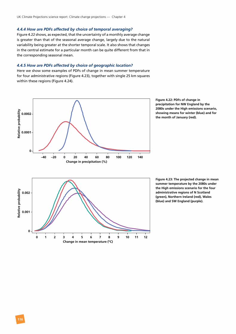
Figure 4.23: The projected change in mean summer temperature by the 2080s under the High emissions scenario for the four administrative regions of N Scotland (green), Northern Ireland (red), Wales (blue) and SW England (purple).

4.4.4 How are PDFs affected by choice of temporal averaging?Figure 4.22 shows, as expected, that the uncertainty of a monthly average change is greater than that of the seasonal average change, largely due to the natural variability being greater at the shorter temporal scale. It also shows that changes in the central estimate for a particular month can be quite different from that in the corresponding seasonal mean.

4.4.5 How are PDFs affected by choice of geographic location? Here we show some examples of PDFs of change in mean summer temperature for four administrative regions (Figure 4.23), together with single 25 km squares within these regions (Figure 4.24).


Rel

ativ

e p

rob

abili

ty

–40 –20 0 20 40 60 80 100 120 140

0.0002

0.0001

0

Figure 4.22: PDFs of change in precipitation for NW England by the 2080s under the High emissions scenario, showing means for winter (blue) and for the month of January (red).

117



Rel

ativ

e p

rob

abili

ty

0.003

0.002

0.001

0

0 1 2 3 4 5 6 7 8 9 10 11 12


Rel

ativ

e p

rob

abili

ty

0.002

0.0015

0.001

0.0005

0

0 2 4 6 8 10 12 14 16 18 20 22 24 26

Figure 4.24: PDFs of change in the mean summer temperature by the 2080s under the High emissions scenario, for four 25 km grid squares including parts of Dorset (purple), Gwynedd (green), Shetland (red) and Co Antrim (blue).

Figure 4.25: Comparison of the PDFs of change in summer mean temperature (green), summer mean daily maximum temperature (blue) and the warmest day of the summer (red) by the 2080s under the High emissions scenario, all for the administrative region of SW England.

Figure 4.23 shows that the distribution of summer mean temperature moves to larger changes, and with correspondingly greater uncertainty, as the location of interest moves from N Scotland to Northern Ireland to Wales and finally to SE England; consistent with the geographical pattern of changes shown by the maps earlier in this chapter. The changes in the 25 km squares within the regions (Figure 4.24) show a similar progression as the regions themselves but some details are different.

4.4.6 How are PDFs affected by choice of mean or extreme variables?Figure 4.25 shows that the most likely change in the summer-mean daily maximum temperature is greater than that in the summer mean temperature. The uncertainty in the warmest day of the summer is much greater than that in the summer-mean daily maximum temperature, which in turn is greater than that in the summer-mean temperature.

118


Mean daily maximum temperature (deg C)

Rel

ativ

e pr

obab

ility

20 22 24 26 28 30 32 34 36 38

0.0.

0005

0.00

10.

0015

High

Plot Details:

Data Source: Probabilistic LandFuture Absolute Climate: TrueVariables: temp_dmax_tmean_absEmissions Scenario: HighTime Period: 2070−2099

Temporal Average: JJASpatial Average: Grid Box 25KmLocation: Grid Box No. 1515Probability Data Type: pdfFontSize: small

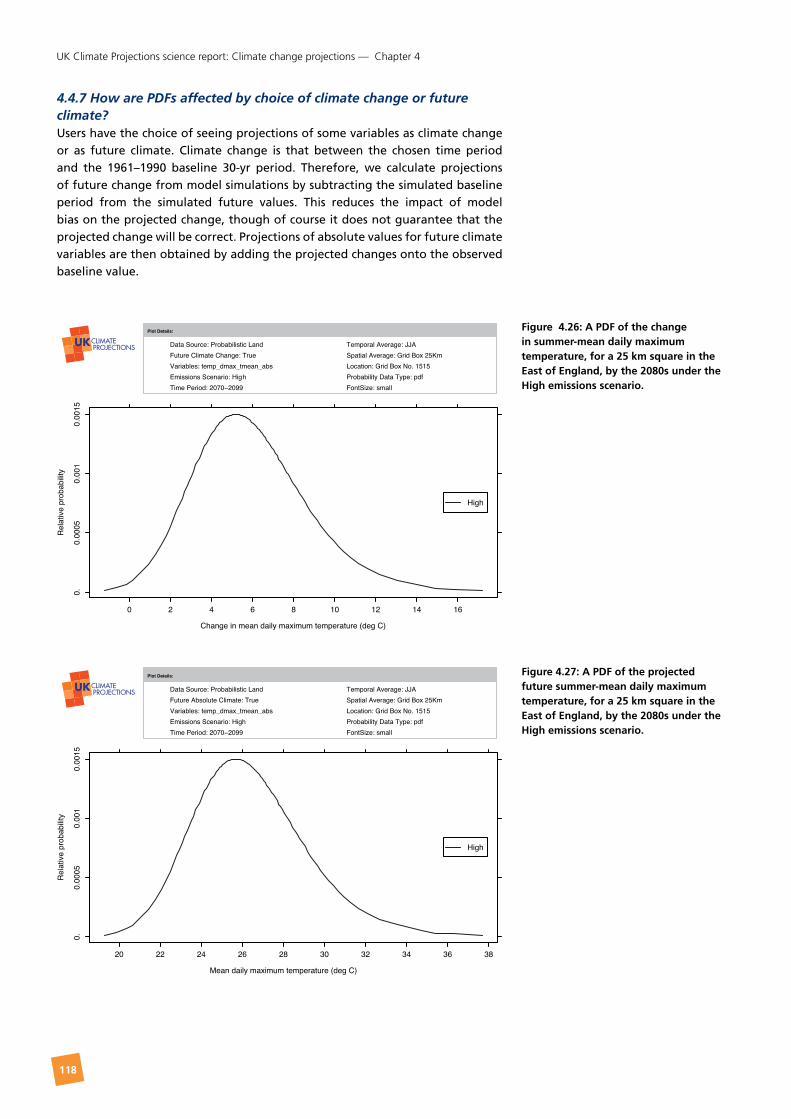
4.4.7 How are PDFs affected by choice of climate change or future climate?Users have the choice of seeing projections of some variables as climate change or as future climate. Climate change is that between the chosen time period and the 1961–1990 baseline 30-yr period. Therefore, we calculate projections of future change from model simulations by subtracting the simulated baseline period from the simulated future values. This reduces the impact of model bias on the projected change, though of course it does not guarantee that the projected change will be correct. Projections of absolute values for future climate variables are then obtained by adding the projected changes onto the observed baseline value.

Figure 4.27: A PDF of the projected future summer-mean daily maximum temperature, for a 25 km square in the East of England, by the 2080s under the High emissions scenario.


Rel

ativ

e pr

obab

ility

0 2 4 6 8 10 12 14 16

0.0.

0005

0.00

10.

0015

High

Plot Details:

Data Source: Probabilistic LandFuture Climate Change: TrueVariables: temp_dmax_tmean_absEmissions Scenario: HighTime Period: 2070−2099

Temporal Average: JJASpatial Average: Grid Box 25KmLocation: Grid Box No. 1515Probability Data Type: pdfFontSize: small

Figure 4.26: A PDF of the change in summer-mean daily maximum temperature, for a 25 km square in the East of England, by the 2080s under the High emissions scenario.

119


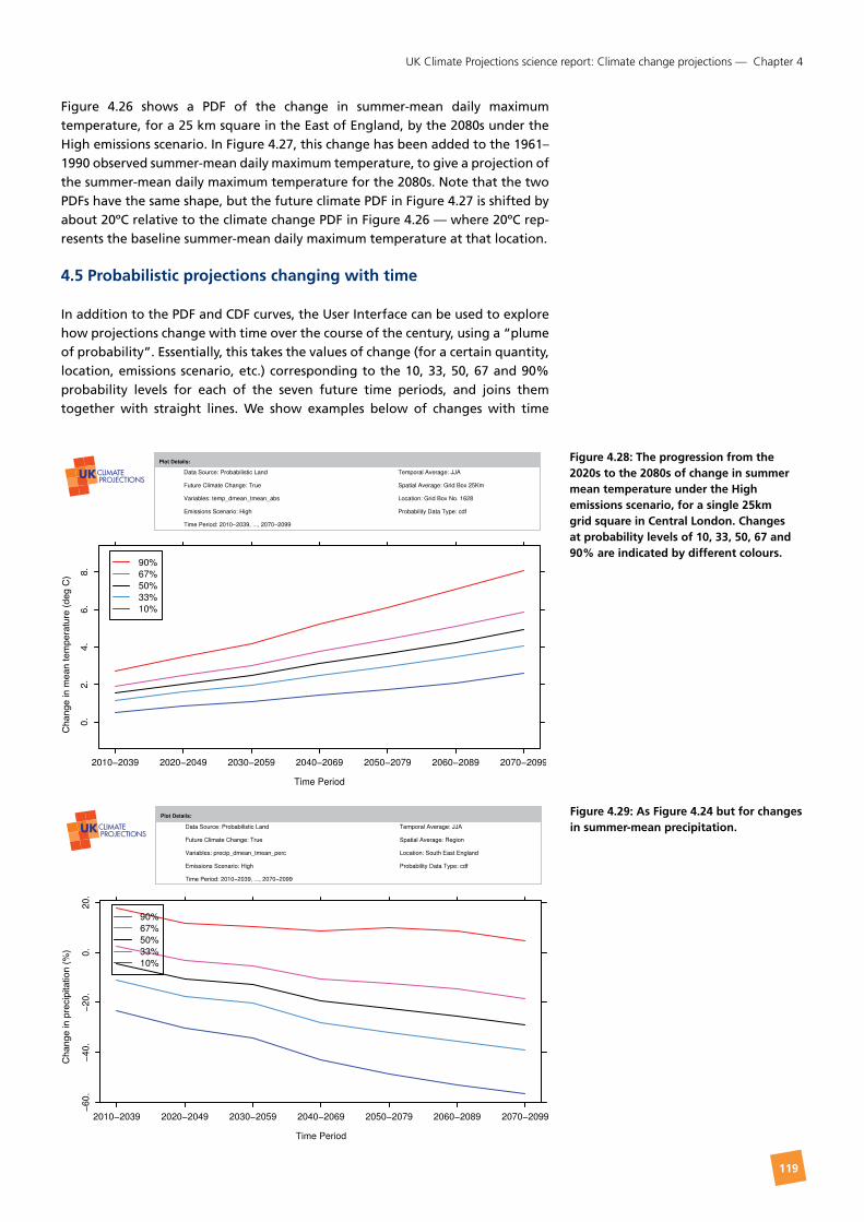
Figure 4.28: The progression from the 2020s to the 2080s of change in summer mean temperature under the High emissions scenario, for a single 25km grid square in Central London. Changes at probability levels of 10, 33, 50, 67 and 90% are indicated by different colours.

Figure 4.29: As Figure 4.24 but for changes in summer-mean precipitation.

Cha

nge

in m

ean

tem

pera

ture

(deg

C)

Cha

nge

in p

reci

pita

tion

(%)

Figure 4.26 shows a PDF of the change in summer-mean daily maximum temperature, for a 25 km square in the East of England, by the 2080s under the High emissions scenario. In Figure 4.27, this change has been added to the 1961–1990 observed summer-mean daily maximum temperature, to give a projection of the summer-mean daily maximum temperature for the 2080s. Note that the two PDFs have the same shape, but the future climate PDF in Figure 4.27 is shifted by about 20ºC relative to the climate change PDF in Figure 4.26 — where 20ºC rep-resents the baseline summer-mean daily maximum temperature at that location.

4.5 Probabilistic projections changing with time

In addition to the PDF and CDF curves, the User Interface can be used to explore how projections change with time over the course of the century, using a “plume of probability”. Essentially, this takes the values of change (for a certain quantity, location, emissions scenario, etc.) corresponding to the 10, 33, 50, 67 and 90% probability levels for each of the seven future time periods, and joins them together with straight lines. We show examples below of changes with time

120


Change in mean temperature (deg C)

Cha

nge

in p

reci

pita

tion

(%)

summer mean temperature (Figure 4.28) and summer mean precipitation (Figure 4.29) for a 25 km square in Central London under the High emissions scenario. Thus the top line in Figure 4.28 shows how the temperature change that is very unlikely to be exceeded increases decade by decade through the century; the middle line shows how the central estimate increases with time, etc. This type of output can be provided by the User Interface for any variable, any emissions scenario and any location.

Plumes show that the width between the 10 and 90% probability levels is already substantial by the 2020s. In the case of precipitation (Figure 4.29), in particular, the width of the plume increases only modestly through the century. The main reason for this is that, at the scale of 25 km, natural internal variability is a big component of the overall uncertainty, and this does not increase with time. Plumes for larger areas (for example, administrative regions) will have a smaller component from natural variability, and do show more growth with time. This reflects the relatively larger components from model uncertainty, carbon cycle feedbacks, etc., which do grow with time. For even larger areas, for example Northern Europe, plumes are even more divergent (not shown here), reflecting the relatively even smaller component of overall uncertainty from natural internal variability at this larger spatial scale.

4.6 The joint probability of the change in two variables

The User Interface allows a calculation to be made, not just of the probability of change in a single variable, but of the joint probability of changes in (some, but not all) combinations of two variables. These can be used to explore specific impacts on targets (such as crops) which are vulnerable to changes in both variables. The User Interface can create plots of joint probability of changes in two variables, chosen by the user, such as that shown in Figure 4.30. This shows an example for two variables commonly used in combination, change in precipitation and that in mean temperature, in summer, by the 2080s under the High emissions scenario. Values of joint probability density are shown by the red contour lines, and have been multiplied by 1000 to make them more readable. So, referring to Figure 4.30, for a precipitation change of –50%, a simultaneous temperature change of 5ºC is about 9 times more likely than a change of 1ºC, as the joint probability densities are 18 and 2 respectively.

Figure 4.30: The joint probability distribution function of changes in summer-mean temperature and that in precipitation, by the 2080s under the High emissions scenario, for the administrative region of Wales. The red lines are contours of probability, multiplied by 1000, with units of per ºC per %. (This plot is direct from the User Interface.)

121


Annex 4 describes the way in which data on the variables is held in batches in the User Interface. Users can explore joint probabilities among those variables in the same batch, but not between variables in different batches. Based on preferences expressed by users, efforts have been made to include within the same batch those variables for which joint probabilities are of particular interest.

4.7 Corresponding changes in global-mean temperature

We have included annual-mean, global-mean temperature as one of the variables for which we make probabilistic projections in UKCP09, although this data is not available from the User Interface. Changes to global mean temperature, for the three emissions scenarios and three future time periods, is shown in Table 4.8.

2020s 2050s 2080s

Emissions 10% 50% 90% 10% 50% 90% 10% 50% 90%

High 1.0 1.3 1.6 2.1 2.7 3.3 3.4 4.3 5.3

Medium 1.0 1.3 1.6 1.9 2.4 3.0 2.6 3.4 4.2

Low 0.9 1.2 1.6 1.6 2.1 2.6 2.0 2.6 3.4

4.8 Variables for which probabilistic projections cannot be provided

For certain variables (soil moisture, latent heat flux, and snowfall rate). it was not possible to provide probabilistic projections of future changes in UKCP09.

In the case of soil moisture, different definitions of this variable are used by different modelling groups, making it impossible to construct PDFs combining results from variants of Met Office models with those from other climate models. Without this key aspect of our methodology, it was not possible to provide probabilistic projections.

In the case of latent heat flux we found that projected changes from two of the alternative climate models were often well outside the range of the Met Office model variants (see Chapter 3, Section 3.2.10). In this situation, our method of combining results from the Met Office model variants and the alternative models could not be guaranteed to provide a robust indication of the probabilities of different outcomes, and hence PDFs were not provided.

In the case of snowfall rate, the models sometimes project small but non-zero values in the future, implying changes relative to the baseline climate that are close to the absolute lower bound of –100%. Under these conditions, statistical contributions to the uncertainties captured in the UKCP09 methodology were found to become unrealistically large, and hence probabilistic projections were not provided.

In the absence of a UKCP09 probabilistic projection for these three variables, there are three possible alternative sources of projections of transient changes during the 21st century:

Table 4.8: The 10, 50 and 90% probability levels of changes to the global mean temperature (ºC), for all three emissions scenarios and three future time periods, as calculated by the UKCP09 methodology.

122


• the 17-member ensemble of variants of the Met Office GCM,

• the 11-member ensemble of variants of the Met Office RCM,

• the ensemble of other global climate models, available from the PCMDI website.

Data from the first two (Met Office GCM and RCM variants) is available from the Climate Impacts LINK project, operated by BADC; see http://badc.nerc.ac.uk/data/link. Data from alternative global climate models can be accessed from the Program for Climate Model Diagnosis and Intercomparison (PCMDI), based in California, which has collected model output from simulations contributed by modelling centres around the world, as part of the Coupled Model Intercomparison Project (CMIP3) of the World Climate Research Programme. The CMIP3 multi-model dataset can be freely accessed for non-commercial purposes via http://www-pcmdi.llnl.gov/ipcc/about_ipcc.php.

Each type of data has advantages and disadvantages. The data from other global climate models, and that from the 17-member Met Office GCM ensemble, is at a relatively coarse resolution. The Met Office RCM has a finer resolution (25 km) and hence provides more information on possible regional variations across the UK. The range of modelling uncertainties explored in the 17-member Met Office GCM ensemble, and the 11-member Met Office RCM ensemble, is not as wide as that explored in the variables for which probabilistic projections are provided in UKCP09. The RCM data is only available for the Medium emissions scenario.

In the case of snow, we recommend the use of changes from the 11-member Met Office RCM ensemble in the first instance. Changes by the 2080s in the winter mean snowfall rate, averaged over the 11-RCM ensemble are shown in Figure 4.31; typically there are reductions of 65–80% over mountain areas and 80–95% elsewhere. Chapter 5 gives details of the data available from the RCM ensemble, its advantages and limitations. Of course, users may wish to extend their analysis, and investigate the robustness of any adaptation decisions, using data from other global climate models. We have not looked at possible alternative projections of soil moisture and latent heat flux, although both are available from the 11-member Met Office RCM ensemble via LINK. It is recommended that users do not revert to UKCIP02 scenarios in isolation, for any of the variables that are not available in UKCP09.

Figure 4.31: Percentage average changes in mean snowfall rate in winter, by the 2080s (relative to 1961–1990) under the Medium emissions scenario, averaged over the 11 members of the Met Office RCM ensemble.

–100 –80 –60 –40 –20 0

Change in snowfall rate (%)

uk climate projections science report: climate change

Documents