Çukurova university institute of natural and applied ... · analiz yöntemi analitik metottur....
TRANSCRIPT

ÇUKUROVA UNIVERSITY INSTITUTE OF NATURAL AND APPLIED SCIENCES
MSc THESIS
Umut ERCAN
MODELLING OF CYLINDRICAL HELICAL SIEVE
DEPARTMENT OF MECHANICAL ENGINEERING
ADANA, 2012

ÇUKUROVA UNIVERSITY INSTITUTE OF NATURAL AND APPLIED SCIENCES
MODELLING OF CYLINDRICAL HELICAL SIEVE
Umut ERCAN
MSc THESIS
DEPARTMENT OF MECHANICAL ENGINEERING
We certify that the thesis titled above was reviewed and approved for the award of degree of the Master of Science by the board of jury on. ………………............ ……......... ………………………….. ……................................ Prof. Dr. İbrahim Deniz AKÇALI Prof. Dr. Vebil YILDIRIM Assoc. Prof. Dr. Ahmet İNCE SUPERVISOR MEMBER MEMBER This MSc Thesis is written at the Department of Institute of Natural And Applied Sciences of Çukurova University. Registration Number:
Prof. Dr. Director Selahattin SERİN Institute of Natural and Applied Sciences
This study was supported by Scientific Research Projects office of Çukurova University (BAP) under grant No. MMF2011YL12 Not:The usage of the presented specific declerations, tables, figures, and photographs either in this
thesis or in any other reference without citiation is subject to "The law of Arts and Intellectual Products" number of 5846 of Turkish Republic
I
ABSTRACT
MSc THESIS
MODELLING OF CYLINDRICAL HELICAL SIEVE
Umut ERCAN
ÇUKUROVA UNIVERSITY INSTITUTE OF NATURAL AND APPLIED SCIENCES
DEPARTMENT OF MECHANICAL ENGINEERING
Supervisor : Prof. Dr. İbrahim Deniz AKÇALI Year: 2012, Pages: 71 Jury : Prof. Dr. Vebil YILDIRIM : Assoc. Prof. Dr. Ahmet İNCE
In this study, the system called cylindrical helical sieve has been undertaken with the purpose of estimating its performance. The method of analysis has been analytical. The sieve has been modeled mathematically with respect to its flow-rate, energy use, efficiency and effectiveness. In another part of the study, an experimental model of the sieve has been set up for measuring flow-rate, energy consumed, effectiveness and efficiency for comparison purposes. In the end, a set of new semi-empirical relationships has been obtained to stand for the performance of the machine, which is supposed to optimize the use of resources. Key Words: Cylindrical sieve, Granular material, Mathematical model, Design
algorithm, Screening conditions.

II
ÖZ
YÜKSEK LİSANS TEZİ
SİLİNDİRİK HELİSEL ELEĞİN MODELLENMESİ
Umut ERCAN
ÇUKUROVA ÜNİVERSİTESİ FEN BİLİMLERİ ENSTİTÜSÜ
MAKİNE MÜHENDİSLİĞİ ANABİLİM DALI
Danışman : Prof. Dr. İbrahim Deniz AKÇALI Yıl: 2012, Sayfa: 71 Jüri : Prof. Dr. Vebil YILDIRIM : Assoc. Prof. Dr. Ahmet İNCE
Bu çalışmada, silindirik helisel elek adı verilen sistemin performansı modellenmiştir. Analiz yöntemi analitik metottur. Eleğin matematik modellenmesi, besleme hızı, verimlilik ve etkili enerji kullanımını içermektedir. Çalışmanın diğer bir noktasında ise, karşılaştırma amaçları için eleğin deneysel bir modeli kurulmuş olup besleme hızı, verimlilik, tüketilen enerji etkin kullanımı laboratuar koşullarında ölçülmüştür. Araştırmanın sonunda, yeni bir makinenin performansını anlatan kuramsal ve deneysel parametrelerin değerleri saptanmıştır. Anahtar Kelimeler: Silindirik Elek, Taneli Ürünler, Matematik Model, Tasarım
Algoritması, Eleme Koşulları.
III
ACKNOWLEDGMENTS
I want to thank to my thesis advisor, Prof. Dr. İbrahim Deniz Akçalı, for his
guidance, support throughout my research. He has been full of ideas, enthusiasm and
always motivating and I enjoyed working with him a lot. I also want to thank, to my
colleagues and my family, especially my mother Kadriye ERCAN, my father Yusuf
ERCAN, my sister Bahar ERCAN for their encouragement and support. I want to
thank to my beloved friend Beyza KÖSE for her patience, inspiration unending love
and support. I would like to thank Prof. Dr. Emin Güzel and Assoc. Prof. Dr. Ahmet
İnce for their support and help.
I also appreciate the support given by MACTİMARUM Research and
Application Center, Laboratory of Agricultural Machinery Department, Cukurova
University.

IV
CONTENTS PAGE
ABSTRACT .............................................................................................................. I
ÖZ ........................................................................................................................... II
ACKNOWLEDGEMENTS..................................................................................... III
CONTENTS ........................................................................................................... IV
LIST OF TABLES .................................................................................................. VI
LIST OF FIGURES ............................................................................................... VII
NOMENCLATURE................................................................................................ XI
1. INTRODUCTION ................................................................................................ 1
2. PREVIOUS STUDIES ......................................................................................... 3
3. MATERIAL AND METHOD............................................................................... 7
3.1. Theoretical Approach ........................................................................................... 7
3.1.1. Cylindrical Helical Sieve System .............................................................. 7
3.1.2. Single Layer Theory ................................................................................... 8
3.1.3. Conditions of Screening ............................................................................16
3.1.4. Machine Design .........................................................................................17
3.1.5. Multi - Layer Theory ................................................................................19
3.1.5.1. The Motion of Multi- Layer Granular Material along a
Circular Path ...................................................................................20
3.1.5.2. The Motion of Multi-Layer Granular Material along a
Helical Path .....................................................................................23
3.2. Formulation of Efficiency ............................................................................ 24
3.3. Experimental Approach ......................................................................................26
3.3.1. Experimental Set - Up ...............................................................................26
3.3.2. Granular Material ......................................................................................27
3.4.3. Measuring Devices ....................................................................................28
3.4.3.1. Cylindrical Helical Sieve System........................................................27
3.4.3.2. Granular Material ...............................................................................28
3.5. Experiments .........................................................................................................34
3.5.1. Equilibrium Angle ....................................................................................34
V
3.5.2. Experiment on Bulk Density ....................................................................35
3.5.3. Experiment for Coefficient of Friction ....................................................35
3.5.4. Efficiency and Flow Rate Experiments ...................................................36
3.5.5. Experiment on Torque ..............................................................................36
3.5.6. Experiment on Power ...............................................................................37
3.5.7. Experiment on Energy ..............................................................................37
4. RESULT AND DISCUSSION ............................................................................ 38
4.1. Equilibrium Angle ...............................................................................................38
4.2. Bulk Density ........................................................................................................45
4.3. Coefficient of Friction .........................................................................................46
4.4. Efficiency and Flow Rate ...................................................................................47
4.5. Torque ..................................................................................................................51
4.6. Power ...................................................................................................................57
4.7. Energy ..................................................................................................................61
5. CONCLUSION .................................................................................................. 65
REFERENCES ....................................................................................................... 67
BIOGRAPHY........................................................................................................ 71

VI
LIST OF TABLES PAGE
Table.3.1. Technical data of Cylindrical helical sieve ........................................... 26
Table 3.2. Lengths of Kidney Beans .................................................................... 27
Table.3.3. Technical data of Power analyzer ........................................................ 28
Table.3.4. Technical data of Torque meter ........................................................... 29
Table 3.5. Technical data of Digital camera ......................................................... 30
Table 3.6. Technical data of Weight scale ............................................................ 31
Table 3.7. Technical Details of Tachometer ......................................................... 31
Table 3.8. Technical Detail of Laptop .................................................................. 33
Table 4.1. Number of layer n=1 ........................................................................... 37
Table.4.2. Theoretical equilibrium angle against number of layer......................... 39
Table. 4.3. Number of layer- result of equation (4.71.) ......................................... 39
Table.4.4. Experimental Values of Equilibrium Angle ......................................... 43
Table.4.5. Semi – empirical relationships between equilibrium angle and number of
layer and feeder gate height. ................................................................ 44
Table.4.6. Mixture Bulk Density .......................................................................... 45
Table.4.7. Coefficient of friction values ............................................................... 45
Table.4.8. Experiment result for 2 cm feeder height ............................................. 46
Table.4.9. Experiment result for 2.5 cm feeder height .......................................... 47
Table.4.10. Experiment result for 3 cm feeder height ............................................. 47
Table.4.11. Experiment result for 3.5 cm feeder height .......................................... 48
Table.4.12. Unloaded Torque Values without Brush .............................................. 51
Table 4.13. Unloaded Torque Values with Brush ................................................... 53
Table.4.14. Loaded Torque Values With Brush ..................................................... 53
Table 4.15. Values of Parameters in Theoretical Torque Calculation...................... 54
Table 4.16. Theoretical Torque Values .................................................................. 54
Table 4.17. Experimental and Theoretical Torque Values due to Load .................. 54
Table 4.18. Experimental Power (Loaded) for Different Feeder Gate Heights ........ 58
Table 4.19. Experimental and Theoretical (Loaded) Power Values vs Feeder
Gate Height ......................................................................................... 59

VII

VIII
LIST OF FIGURES PAGE
Figure 3.1. Cylindrical Helical Sieve ................................................................... 8
Figure 3.2. The circular motion of a single item ................................................... 9
Figure 3.3. Circular motion of the layer of granular material ................................ 10
Figure 3.4. Helical motion of a single item ........................................................... 12
Figure 3.5. Velocity components.......................................................................... 14
Figure 3.6. Geometry of the layer between two helices ........................................ 15
Figure 3.7. Motion of a single item by the sieve hole ........................................... 15
Figure 3.8. Multilayer granular material in cylinder ............................................. 19
Figure 3.9. Layer thickness variation in terms of developed arc ........................... 20
Figure 3.10. Efficiency of the separation process ................................................... 23
Figure 3.11. Power quality analyzer ....................................................................... 27
Figure 3.12. Torque meter...................................................................................... 29
Figure 3.13. Digital camera .................................................................................... 30
Figure 3.14. Weight scale ...................................................................................... 31
Figure 3.15. Digital tachometer .............................................................................. 32
Figure 3.16. Meter ................................................................................................. 32
Figure 3.17. Chronometer ...................................................................................... 32
Figure 4.1. Theoretical equilibrium angle ............................................................. 38
Figure 4.2. Theoretical equilibrium angle vs. Number of layer ............................. 39
Figure 4.3. dβ/dn vs number of layer .................................................................... 40
Figure 4.4. Equilibrium Angle for 2cm feeder gate height .................................... 41
Figure 4.5. Equilibrium Angle for 2.5cm feeder gate height ................................. 41
Figure 4.6. Equilibrium Angle for 3cm feeder gate height .................................... 42
Figure 4.7. Equilibrium Angle for 3.5cm feeder gate height ................................. 42
Figure 4.8. Equilibrium angle- feeder gate heights ............................................... 43
Figure 4.9. Number of layer vs. feeder gate heights .............................................. 44
Figure 4.10. Measured bulk density vs small size ratio ........................................... 45
Figure 4.11. Efficiency vs small - size ratio ........................................................... 48
Figure 4.12. Mass flow rate vs small - size ratio ..................................................... 49

IX
Figure 4.13. Efficiency vs mass flow rate .............................................................. 50
Figure 4.14. Experimental torque values Vs feeder gate heights ............................. 53
Figure 4.15. Experimental torque due to load vs. feeder gate height ....................... 53
Figure 4.16. Theoretical torque vs. number of layer .............................................. 55
Figure 4.17. Theoretical torque values vs. feeder gate heights ................................ 55
Figure 4.18. Experimental and theoretical Torque values due to load vs. feeder gate
heights .............................................................................................. 56
Figure 4.19. Experimental power with and without brush vs. time ......................... 57
Figure 4.20. Experimental power vs. time for different feeder gate heights ............ 57
Figure 4.21. Power due to load vs time .................................................................. 58
Figure 4.22. Experimental power values vs. feeder gate heights ............................. 58
Figure 4.23. Theoretical power values vs. feeder gate heights ................................ 59
Figure 4.24. Power values vs. feeder gate heights .................................................. 59
X
NOMENCLATURE
sheet metal thickness ( ) infinitesimal mass of layer per unit length ( / ) ⁄ mass flow rate along cylinder axis ( / ) diameter of helicoid piece ( ) external diameter of ring ( ) internal diameter of ring ( ) thickness of layer ( )
E energy consume (kWs) net force (N) gravitational acceleration ( / ) power ( ) ℎ pitch ( )
h layer thickness (-)
K, B small and big size group (g) , hole width and length ( )
n number of layer (-) cylinder radius ( ) ̈ acceleration of item ( / ) ̈ , ̈ accelerations along circular and helical paths ( / )
T total mass (g) moment about cylinder axis per unit length (Nm/m) relative velocity along helical path ( / ) transport velocity of granular material along the cylinder axis ( / ) tangential cylinder velocity ( / )
y co-ordinate axis along gravitational acceleration (m)
z co-ordinate axis along the cylinder axis (m) angular velocity (r/s) width of helicoid piece ( )

XI
∗ angles which the single item starts sliding motion ( o ) ∗ angle at which sliding occurs along circular paths ( o ) ∗ angle at which sliding occurs along helical paths ( o ) equilibrium angle ( ) , equilibrium angles for motion along circular, helical paths ( ) density of granular material ( / ) coefficient of friction between item and cylinder surface ( - ) coefficient of friction between item and helicoid surface ( - ) , ′ helix angle and its complementary ( o ) η , η small and big size efficiency η overall efficiency

1. INTRODUCTION Umut ERCAN
1
1. INTRODUCTION
Sorting is the separation of foodstuff into categories on the basis of a
measurable physical property (Fellows, 2000). Like cleaning, sorting should be
employed as early as possible to ensure a uniform product for subsequent processing.
The main objective of sorting is to provide uniformity over the food raw material,
which is often said to be preferred by consumers. Other advantages of sorting is to
secure product standardization, efficiency in subsequent processing of raw foodstuff
and to make it possible to express other characteristics by means of the fundamental
physical parameter.
Shape sorting is useful in case where the granular materials are contaminated
with particles of similar size and weight. The principal disc or cylinders with
accurately shaped indentations will pick up seeds of the correct shape when rotated
through the stock, while other shapes will remain in the feed.
Size sorting, which is the separation of solids into two or more fractions on
the basis of differences in size, is one of the frequently used processes in the
preparing of food. Sorting into size categories requires different type of screens.
Colour sorting method can also be used to separate materials which are to be
processed separately, such as red and green tomatoes. It is feasible to use
transmittance as a basis for sorting, although as most foods are completely opaque,
very few opportunities are available. The principle has been used for sorting cherries
with and without stones and for the internal examination, or candling of eggs.
Grading is classification on the basis of quality incorporating commercial
value, end use and official standards and hence requires that some judgments on the
acceptability of the food is made, based on simultaneous assessment of several
properties, followed by separation into quality categories (Grandison, 2006).
Appropriate inspection belts or conveyors are designed to present the whole surface
to the operator. There is much interest in the development of rapid, nondestructive
methods of assessing the quality of foods, which could be applied to the grading and
sorting of foods, the potential application of advanced optical techniques to give
information on both surface and internal properties of fruits, including textural and

1. INTRODUCTION Umut ERCAN
2
chemical properties. This could permit classification of fruit in terms of maturity,
firmness or the presence of defects, or even more specifically, the noninvasive
detection of chlorophyll, sugar and acid levels. Another promising approach is the
use of sonic techniques to measure the texture of fruits and vegetables. Similar
applications of X-rays, lasers, infrared rays and microwaves have also been studied.
Computer vision has been used for such tasks as shape classification, defect
detection, quality grading and variety classification.
The objective of this thesis is to investigate analytically the sorting function
of a system called cylindrical helical sieve. Here, the motion of granular material has
been modeled in cylindrical medium rotated at a constant angular velocity on the
basis of single item and of multilayer of granular material guided along circular,
helical and combined paths. Efficiency, torque, power and energy experiments have
been done. Experimental and theoretical results have been compared with each other.
Finally, the optimum operating conditions of the cylindrical helical sieve have been
determined.

2. PREVIOUS STUDIES Umut ERCAN
3
2. PREVIOUS STUDIES
A wide range of mechanical separation equipment is used in food processing.
Some basic equipment, such as vibrating screens, optical sorting, colour sorting, and,
are adapted from the food process industry. Fundamental food processing research is
focused on the physical and engineering properties of foods, which are required in
the quantitative design of food processes, food processing equipment.
The type of driving mechanisms in relation to performance of vibrating screen
has been the subject of many studies. For instance, in one of them (Tan & Harrison,
1987) influence of several different planar and spatial drive mechanisms on the
screening efficiency has been worked out to obtain optimum performance in terms of
the so called screening index. Yet in another work (Shen et al., 2009), a novel
vibration sieve mechanism using a parallel mechanism has been proposed. Here
optimum design based on structure, kinematic analysis and motion simulation has
been demonstrated. The motion of granular material has also been analyzed in
another work (Hongchang et al., 2011) with respect to a performance parameter
called throwing index .In this analysis the most suitable value of throwing index has
been found corresponding to the best performance of vibration screen.
The vibrating screen has found extensive applications in many different
industries. For instance, in coal processing in mining science, vibrating screens have
been taken into account from the standpoint of their “ideal motion” with the purpose
of improving processing capacity and efficiency within the frame work of computer
models (He & Liu, 2009).Vibrating screen with variable elliptical trace has been
proposed resultantly. Another work for computer model of sieves’ vibrations analysis
has been done in civil engineering construction bulk material screening using an
algorithm based on the so-called false-position method (Stoicovici et al., 2009).
There have been some works related to the vibratory motion of the granular
material using the so-called discrete element method. For instance, screening
phenomena has been analyzed in another mechanical environment called vertical
tumbling cylinder (Alkhaldi & Eberhard, 2006), whereby the concept of discrete
element method (DEM) that considers the motion of each single particle individually

2. PREVIOUS STUDIES Umut ERCAN
4
has been applied. A numerical study of the motion particulates along a circularly
vibrating screen deck has been done using the three dimensional Discrete Element
Method (DEM) (Lala et al., 2011). Here the effect of vibration amplitude, throwing
index and screen deck inclination angle on the screening process has been
determined for optimizing screen separator designs.
Optimization of vibrating screen has also been carried out using commercial
software such as Matlab (Shuang & Nian-qin, 2010). In this study, on the basis of
basic demand for vibration screen with high productivity, the mathematical model
with maximum efficiency targets has been established while premising the screening
productivity, and the optimization system.
This study point out that changing the position of components, although the
all loads and all other dimensions remain the same; can have serious implication on
the fatigue life of a component. Fatigue failure of deck support beams on a vibrating
screen was surveyed by Jacques Steyn (Steyn, 1995).
Another study is dynamic design theory and application of large vibrating
screen was design by Zhao Yue-min et al. (Zhao et all. 2009). They have used Finite
Element Method (FEM) to analyze dynamic characteristic of large vibrating screen
with hyperstatic net-beam structure. The structural size of stiffeners on the side plate
was optimized under multiple frequencies constraints and an adaptive optimization
criterion was given.
There are several studies in the literature that focus up on vibrating screen for
maximization. For instance, research on dynamic characteristics of elliptical
vibrating screen has been undertaken by utilizing finite element software ANSYS to
carry on modal analysis and dynamic stress analysis of elliptical vibrating screen,
and finds out the dynamic stress distribution and modal parameters (Zhongjun et all.
2010). Another study is parameters optimum design for linear vibrating screen in
which mathematical model of linear vibrating screen with the pursuit of minimum
power consumption per productive has been established using MATLAB software
(Yan et all. 2010).
There are various systems utilizing image processing techniques. Computer
vision systems have been used increasingly in industry for inspection and evaluation
2. PREVIOUS STUDIES Umut ERCAN
5
purposes as they can provide rapid, economic, hygienic, consistent and objective
assessment. However, difficulties still exist, evident from the relatively slow
commercial uptake of computer vision technology in all sectors (Ata et all. 2005) For
instance, colour recognition using fiber optic cabled sensors interfaced with robot
controller and Programmable Logic Controller (PLC) in robotics application has
been discussed (Brosnan, & Sun 2002).The aim of this research work is to recognize
colour by pin point detection and sorting of object specimens with respect to their
colour attributes, which includes hue, saturation and luminance level. Another study
is inspection and grading of agricultural and food products by computer vision
systems-a review. This study focuses on the progress of computer vision in the
agricultural and food industry then identifies areas for further research and wider
application of the technique. According to the Guang-rong L.,( Guang-rong 2010)
color of rice is an important indicator of rice grade; this article has provided an
objective and accurate way to inspect the rice color based on image processing
technique . It has been shown that the application of two popular kinds of color
model, Red, Green, Blue (RGB) model and H (hue), S (color saturation) and I
(brightness) HSI model is feasible, in the rice color inspection. Computer vision has
been used for such tasks as shape classification, defect detection, quality grading and
variety classification.
Including the inspection of quality and grading of fruit and vegetable, non-
destructive method of inspection has found applications in the agricultural and food
industry. One study (Narendra & Hareesh, 2010) reviews the progress of computer
vision in the agricultural and food field then explores different possible areas of
research having a wider scope to enhance the existing algorithms to meet the today’s
challenges. Another study (Brosnan & Sun, 2004) has reported the recent
developments and applications of image analysis in the food industry, the basic
concepts and technologies associated with computer vision.
Grading method has been applied to Jonagold apples. Several images
covering the whole surface of the fruits were acquired thanks to a prototype grading
machine. Each blob was then characterized by 15 parameters: five for the colour,
four for the shape, five for the texture and only one for its position. These images
2. PREVIOUS STUDIES Umut ERCAN
6
were then segmented and the features of the defects were extracted. The prior step is
the images acquisition, which was performed by Charge Coupled Device (CCD)
cameras during the motion of the fruit on an adapted commercial machine. It was
followed by a first segmentation to locate the fruits on the background and a second
one to find the possible defects. Once the defects were located, they were
characterized by a set of features including colour, shape, texture descriptors as well
as the distance of the defects to the nearest calyx or stemend. The correct
classification rate of Jonagold apples was of 73% (Unay & Gosselin 2004). In view
of the lower efficiency despite the increasing number of parameter it is understood
that in order to get better results, wavelength process could be offered to get better
results.
Through the latest NIR (Near Infra Red) technology, packhouses can now
sort their produce not just by size and color, but by indicators of produce taste. This
is done without damaging produce as no mechanical mechanism touches the
individual fruit. Brix is a measure of the percent of solids in a given weight of plant
juice. It is often expressed as equaling the pounds of sucrose, fructose, vitamins,
minerals, amino acids, proteins and other solids in one hundred pounds of a
particular plant juice (Compact sorter).
The objective of this thesis is to investigate analytically the sorting function
of a system called cylindrical helical sieve. Here, the motion of granular material has
been modeled in cylindrical medium rotated at a constant angular velocity on the
basis of single item and of multilayer of granular material guided along circular,
helical and combined paths. Efficiency, torque, power and energy experiments have
been done. Experimental and theoretical results have been compared with each other.
Finally the effectiveness of the sorting system has been explained.

3. MATERIALS AND METHOD Umut ERCAN
7
3. MATERIALS AND METHOD
In this study, firstly operation of sieve machine has been described. The sieve
has been modeled mathematically with respect to its mass flowrate, energy use,
efficiency and effectiveness. The mathematical model has been transformed into
design algorithm. Finally, efficiency, mass flow rate, energy consumption and torque
experiments have been done. Materials used in experiments have been characterized.
Experiment material has been identified. The substance of this section is presented in
two categories. One of them is the theoretical approach applied to the sieve machine
and the other is the experimental approach to prefer it’s perform.
3.1. Theoretical Approach
In theoretical approach, the sorting system called helical cylindrical sieve is
described briefly. Then single – layer and multi – layer theories will be developed for
the modeling of the system.
3.1.1. Cylindrical Helical Sieve System
The system shown in Figure 3.1 consists of two fundamental parts. One of
these is the feeder and the other is cylindrical helical sieve. There are two sided
brushes which are placed in parallel with the axis of the cylinder. These brushes are
utilized to prevent blockage of the sieve holes. On the other hand, power
consumption is supposed to increase because of to brushes. Power is provided by the
electrical motor, and is transferred to the shaft of cylindrical sieve by belt-pulley
system. As the cylinder rotates about its axis, the gate of the feeder is vibrated at the
same time through a cylindrical cam mechanism to start the flow of the agriculture
material into the sieve. Underneath the cylindrical sieve there exists a box for
collecting the small-size material as well as another box for collecting big size
material from the end of the sieve.
3. MATERIALS AND METHOD Umut ERCAN
8
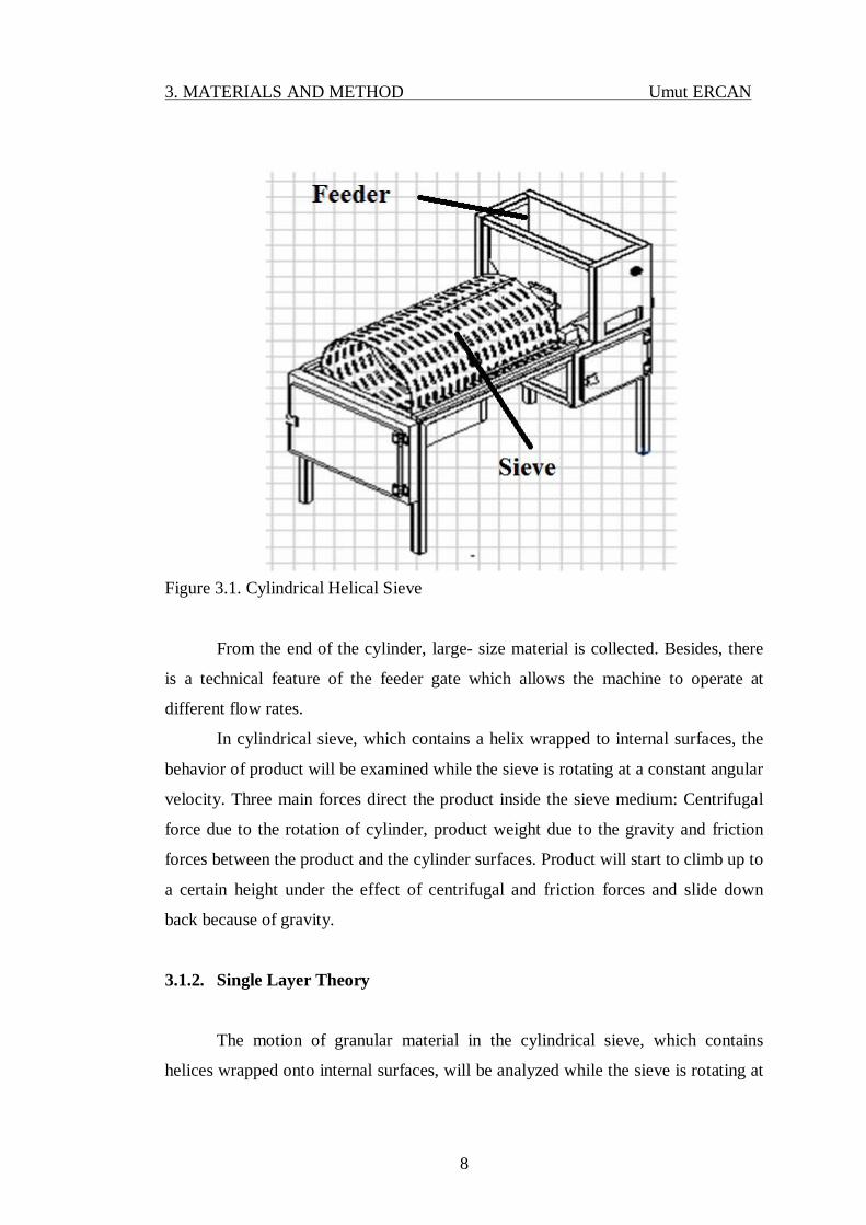
Figure 3.1. Cylindrical Helical Sieve
From the end of the cylinder, large- size material is collected. Besides, there
is a technical feature of the feeder gate which allows the machine to operate at
different flow rates.
In cylindrical sieve, which contains a helix wrapped to internal surfaces, the
behavior of product will be examined while the sieve is rotating at a constant angular
velocity. Three main forces direct the product inside the sieve medium: Centrifugal
force due to the rotation of cylinder, product weight due to the gravity and friction
forces between the product and the cylinder surfaces. Product will start to climb up to
a certain height under the effect of centrifugal and friction forces and slide down
back because of gravity.
3.1.2. Single Layer Theory
The motion of granular material in the cylindrical sieve, which contains
helices wrapped onto internal surfaces, will be analyzed while the sieve is rotating at

3. MATERIALS AND METHOD Umut ERCAN
9
a constant angular velocity. The study will be carried out basically in two steps: In
the first step, the motion of a single item will be investigated. In the second step, the
motion of granular material layer as a group will be studied. Here, it will be assumed
that the granular material covers the internal surface of the cylinder continuously in
the form of a single layer.
Three main forces which govern the motion of the material inside the sieve
medium are the centrifugal force on the material resulting from the rotation of
cylinder, material weight due to the gravitational acceleration and friction forces
between the single granular material and the interacting surfaces. Granular material
(one by one or in groups) will be carried by the rotating cylinder to a certain height
under the effect of centrifugal and friction forces, and then will slide downwards
from that height because of gravity.
Now, mathematical theory of the motion of granular material will be
presented according to paths followed by either a single item or as a layer:
3.1.2.1. The Motion of one Single Item along a Circular Path
One of the paths along which a single item is supposed to move is a circular
arc on the internal surface of a cylinder with radius , which is rotated with angular
velocity . Referring to Fig. 3.2, application of Newton’s Second Law will lead to
the following expression for the acceleration of the item:
Figure 3.2. The circular motion of a single item ̈ = sin − cos − (3.1.)
In equation (3.1.) is the coefficent of friction between the cylindrical
surface and granular material.

3. MATERIALS AND METHOD Umut ERCAN
10
In order to determine the angle ( ∗) at which downward sliding motion starts,
it is necessary that the following condition be satisfied: ̈( ) > ̈( ∗) = 0 (3.2.)
From which, ∗ = 2 ( ⁄ ) ( )⁄ (3.3.)
From a review of equation (3.3.) for ∗ > 0, it follows:
< (3.4.)
Relationships (3.2.) - (3.4.) reveal that sliding motion will occur when > ∗ .
3.1.2.2. The Motion of Layer of Granular Material along a Circular Path
If the layer of granular material assumed to cover the internal surface of the
cylinder is to come to equilibrium at angle of then from Fig. 3.3 the following can
be written: = ∫ ̈ = 0 (3.5.)
In equation (3.5.) is the net force which moves the layer downwards, ̈
represents the acceleration of the infinitesimal mass with size . Besides,
designating the bulk density of the granular material by , and the thickness of the
layer by , infinitesimal mass of the layer per unit length ( ) can be expressed as
follows:

3. MATERIALS AND METHOD Umut ERCAN
11
Figure 3.3 Circular motion of the layer of granular material = or = (3.6.)
Substituting (3.6.) in (3.5.) and carrying out integration, one obtains the following
equation: (1 − )− − = 0 (3.7.)
Equation (3.7.) is a nonlinear algebraic equation in the unknown which
requires numerical solution. Nevertheless for small angles an initial solution to
start a numerical iteration procedure can be found as follows. ≈ or ≈ 1 − / 2 (3.8.) 2⁄ − ( 1 + ⁄ ) = 0 (3.9.)
Or = 0 , = 2 (1 + )⁄ (3.10.)
If relationship (3.4.) is taken into account, the following results: < 4 (3.11.)
In order to determine the location ( ∗) of the center of gravity of the layer, the
following can be written: ∫ = ∗ (3.12.)
From equation (3.12.) the following is deduced: ∗ = (1− )/ (3.13.)
Using (13), moment about the cylinder axis ( ) per unit length of the covered
material can be computed by the following equation.

3. MATERIALS AND METHOD Umut ERCAN
12
= (1− ) (3.14.)
Resultantly, the power ( ) required to move the layer along the circular path is
estimated by the following: = (3.15.)
Energy use due to a single layer transported material in the time interval [t0, tn] is
evaluated by the following: = ∫ (3.16.)
3.1.2.3. The Motion of a Single Item of Granular Material Along a Helical Path
Referring to Fig. 3.4, the helix angle between the cylinder axis and the helical
path, and its complementary angle are designated by , ′ respectively.
Considering that single item of granular material follows the line joining the helicoid
and the internal cylindrical surface, the motion of the single item will be resisted by
friction forces on these surfaces. Assuming that the coefficient of friction between
the item and the cylinder surface is represented by and that between item and
helicoid is , then the downward acceleration ( ̈) of the sliding item turns out to be
the following:
Figure 3.4.Helical motion of a single item ̈( ) = sin ( − ) − cos − (3.17.)
In accordance with condition (3.2.), the angle ( ∗) at which the single item
starts sliding along the helical path is found by the following equation: ∗ = 2 ( √ ) (3.18.)

3. MATERIALS AND METHOD Umut ERCAN
13
where = ( − ) , = , = (3.19.)
The conditions of sliding motion of the single item along the helical path can
be determined by examining equation (3.18.): These conditions are firstly, the
limitation of the angular speed of the cylinder as implied by condition (3.4.), which
shows the angular speed preventing the sticking of material onto the inner surface at
the top. Secondly, the relationship between the helical angle and the coefficient of
friction can be deduced as follows: < 1 ⁄ or tan > (3.20.)
3.1.2.4. The Motion of Layer of Granular Material along a Helical Path
The fundamental purpose of investigating the bulk motion of the granular
material is to determine the amount of granular material to be transported along the
cylindrical axis per unit length of the cylinder. It has been shown that a certain
relationship can be observed between the circular and the helical motions of the
single item. Based on this observation, a similar relationship is expected between the
circular and helical motion of bulk material. Comparing circular and helical motions
of the single item, conclusions as to how layer of granular material moves along
helical path can be drawn.
Based on this comparison, it can be said that the sliding acceleration along the
helical path at the same position ( ) will be seen to be smaller than that in the case of
circular path. In other words, the angle at which sliding will occur for the helical path
will be seen to be larger relative to the circular case, due to the fact that: − < 1 (3.21.)
Accordingly, the area of inner cylinder surface covered by the granular
material will be larger in the case of helical path as is easily understood from the
larger angle. This is to mean that the mass flow rate of the transported granular
material corresponding to helical path will be larger than that of circular path.

3. MATERIALS AND METHOD Umut ERCAN
14
Nevertheless, if the assumption that granular material is supposed to continuously
cover the inner surface of the cylinder in the form of a single layer is reviewed, it
will be realistic to think that some probable gaps will be formed during the motion
along the helical path, leading to a more realistic estimation of the mass flow rate by
means of circular path case.
To support the discussion above, it is sufficient to note that the angle ( )
which results from equation (3.5.) for the case of helical path becomes the following: (1 − )( − ) − ( + ) = 0 (3.22.)
Although there is no precise analytical solution of equation (3.22.), for small
angles ( ) the root of (3.22.) with technical meaning is the following: = (1 + ) (3.23.)
Now, designating transport velocity of the granular material along the
cylinder axis by , relative velocity along the helical path by and the tangential
cylinder velocity by the following vector equation can be written:
Figure 3.5. Velocity components = + (3.24.)
Referring to Fig. 3.5 and to the geometry of the cylinder (Fig. 3.4) the
following scalar relationships result: = (3.25.) = ⁄ (3.26.) = tan (3.27.)
Consequently, mass flow rate per unit length along the cylinder axis is
expressed by the following equation:

3. MATERIALS AND METHOD Umut ERCAN
15
⁄ = (3.28.)
3.1.2.5. Granular Material Motion for Combined Circular - Helical Paths
The case considered here is the one whereby layer supposed to move along
circular path is forced to move along a helical path. This case concerns the motion in
the area between two helicoids attached to the inner surfaces of the cylinder. The
sliding conditions are between the two limiting conditions of the circular and helical
cases established previously. If the symbols ∗ , ∗ represent the angles at which
sliding occurs along circular and helical paths, respectively, sliding angle ∗ corresponding to combined circular – helical path and the relevant acceleration ̈( ) are bounded by the following relationships.
∗ < ∗ < ∗ (3.29.) ̈ ( ∗) < ̈ ( ∗) < ̈ ( ∗) (3.30.)
where ̈ , ̈ designate the accelerations along helical and circular paths,
respectively.
Under the case considered the angle ( ) at which the layer of granular material
comes to equilibrium inside the rotating cylinder, will be affected. If , ,
represent the equilibrium angles for motion along circular, helical and combined
paths respectively, the following inequality can be written:
< < (3.31.)
Figure 3.6. Geometry of the layer between two helices

3. MATERIALS AND METHOD Umut ERCAN
16
What inequality (31) implies is depicted in Fig. 3.6.
3.1.3. Conditions of Screening
The basic principle underlying size sorting is that an item of a particular size
falls into the relevant section by passing through the holes of the screen.
Nevertheless, in order for the principle to be materialized, the control over item
velocity is essential.
For the purpose of mathematically deriving the expressions related with the
velocity control, an item is shown in Fig.3.7 at an initial position before entering the
hole of the screen.
Figure 3.7. Motion of a single item by the sieve hole
If Newton’s Second Law is written for the motion of the item in the and
axes, Fig. 6, the following equations result:
= 0 , = (3.32.)
Assuming that the item has velocity and zero displacement initially, the
solutions of equation set (3.32.) will be following: = , = (3.33.)
or = (2 )⁄ (3.34.)
Now, the condition for the item to pass through the hole without hitting its
lower corner can be established as such: ≥ + , = (3.35.)

3. MATERIALS AND METHOD Umut ERCAN
17
where, , , are the sheet metal thickness, item thickness, hole length,
respectively. If conditions (3.35.) are evaluated in equation (3.34.), the following
result is obtained:
≤ ( ) (3.36.)
It means that the item velocity in the z direction should be governed by the
relation (3.36.).
Similarly, the tangential velocity ( ) in the direction perpendicular to
cylinder axis should be limited through the following relationship:
≤ ( ) (3.37.)
where , are the width of hole and tangential velocity, respectively.
Relationships (3.36.) - (3.37.) imply that the item should have limited
velocities along the cylinder axis as well as perpendicular to it for effective
screening.
3.1.4. Machine Design
3.1.4.1. Design Principles
In the formation of a design procedure for the cylindrical helical sieve which is
to be used for size sorting, the mathematical foundation previously established will
be taken into account. This mathematical foundation associates the physical
properties of the granular material with the design parameters. The design parameters
in question are fundamentally shape and dimensions of screen, cylinder radius,
angular velocity, axial velocity of the granular material, cylinder length. The basic
physical properties of the granular material are namely, the coefficient of friction
with the screen material and the helicoid surface, density, length and thickness of the
grain. Besides, the other auxiliary quantity which goes into the design procedure is

3. MATERIALS AND METHOD Umut ERCAN
18
the angle of equilibrium ( ), which is commonly determined by the granular material
properties and the machine characteristics.
Another factor to be taken into consideration in the design is the dimensions of
the helicoid surface to be placed inside the cylindrical surface. For all practical
purposes, in terms of the diameter ( ), pitch (ℎ), width ( ), the internal ( ), and
external ( ) diameters of the ring which will form the helicoid are calculated as
follows:
= + ℎ , = − 2 (3.38.)
3.1.4.2. Design Technique
The mathematical model developed previously will be transformed into a
number of ordered steps to form an algorithm yielding the values of the design
parameters. In this way, a design technique readily applicable to a computer has
come out. Below are given the ordered steps:
i. Desirable mass flowrate and the physical properties of the granular
material are entered.
ii. The width and the length of the oblong hole of the sheet metal are
selected according to the classification table of granular material. For
instance, the references (Guzel et al., 2005; Guzel et al., 2007; Akcali &
Guven, 1990; Akcali et al., 2006) are to be referred to when the granular
material is peanut.
iii. Helix angle is selected so as to satisfy inequality (3.20.).
iv. Taking into account the sheet metal size corresponding to cylinder radius
and length are chosen; and thickness of sheet metal is entered.
v. An angular speed satisfying relation (3.4.) is assumed.
vi. Angle of equilibrium is found by an iteration technique using equation
(3.7.) and initial solution (3.10.).
vii. Axial velocity of the granular material is computed by equation (3.27.).

3. MATERIALS AND METHOD Umut ERCAN
19
viii. Mass flowrate is calculated by means of equation (3.28.) and the relevant
data.
Until the desirable mass flowrate is satisfied the following steps are
iterated:
a. Steps starting from number v are repeated.
b. If the steps in the previous iteration (a) do not satisfy the basic
mass flowrate criterion, steps starting from number iv are repeated.
c. In case the mass flowrate criterion is not satisfied in the previous
step (b), then iteration is started from number iii thereafter.
d. If the basic mass flowrate criterion is still not satisfied in the
previous step (c) then iteration is executed from step number ii.
ix. After having approximately obtained equality between desirable and
actually calculated values of mass flowrate, the axial velocity is checked
with respect to screening condition (3.36.). If the condition (3.36.) has not
been realized, the new length of the hole is selected in step number ii and
the following steps are iterated until the condition is satisfied.
x. Tangential velocity of the granular material is computed by equation
(3.25.) and all the steps starting from number iv are executed until
condition (3.37.) is satisfied.
3.1.5. Multi - Layer Theory
Observations in the operation of the machine show that single layer of granular
material cannot be maintained throughout the motion of the granular material on the
internal surface of the cylinder. Since the efficiency is lower than one hundred
percent, this situation is attributed to the formation of layers, one grain on top of the
other, a condition underlying the observed loss in the efficiency by preventing the
contacting of the above grain from the surface of the cylinder. Thus in order to model
the operation of the system realistically there is a need to develop multi layer theory.
3. MATERIALS AND METHOD Umut ERCAN
20
The methodology followed for single layer theory will be utilized taking into
consideration the varying thickness of the layer.
3.1.5.1. The Motion of Multi- Layer Granular Material along a Circular Path
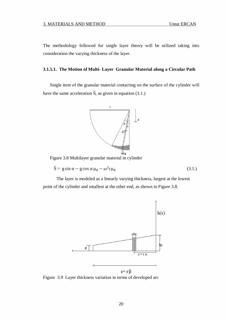
Single item of the granular material contacting on the surface of the cylinder will
have the same acceleration S̈, as given in equation (3.1.)
Figure 3.8 Multilayer granular material in cylinder S̈ = g sin α − g cos αμ −ω rμ (3.1.)
The layer is modeled as a linearly varying thickness, largest at the lowest
point of the cylinder and smallest at the other end, as shown in Figure 3.8.
Figure 3.9 Layer thickness variation in terms of developed arc

3. MATERIALS AND METHOD Umut ERCAN
21
Referring to Fig.3.9 if the thickness is h when the angular position α is zero
and e at the other hand when α is β, then by designating the developed distance
from the lowest point of the cylinder upward by s, then the following boundary
conditions can be written for layer thickness h in terms of s: h(s) = h at s = 0 , ( α = 0) (3.39.) h(s) = e at s = βr , ( α = β) (3.40.)
Assuming a linear equation as such: h = a + bs (3.41.)
The coefficient a and b can be determined by using boundary conditions (3.39.) and
(3.40.). The following results are obtained: a = h (3.42.) b = (3.43.)
h(s) = h − (3.44.)
By using the relationship between developed distance ( s ) and angular position (α)
i.e. s = r α , the following forms of layer thickness h can be given: h(α) = e[n− (n− 1) ] (3.45.)
h(s) = e[n− ( ) s ] (3.46.)
= (3.47.)
where n is the number of layers of the granular material. Infinitesimal mass of the
layer per unit length of the cylinder at angular position (α) is formulated as such: dm = ρ h r dα
(3.48.)
If equation (3.45.) is used in equation (3.48.) and integrated between 0 and
equilibrium angle β, the following result is obtained:

3. MATERIALS AND METHOD Umut ERCAN
22
m = ρr β = ( ) ρr β (3.49.)
If equilibrium condition (3.5.) is used together with infinitesimal mass expression
(3.48.) and integration is carried out between 0 and angle β the following equation
results: F = ρ r[ (−2 g μ + r w β μ + 2 g (β+ μ ) cosβ +2 g (β μ − 1) sinβ − 2 (r w β μ − g + g cosβ + (g μ h sinβ)] (3.50.)
In order to find equilibrium angle β, when F = 0 , the following function can be
formed: F(β) = g [( β(n− cosβ) − (n− 1)sinβ)]− g μ β sinβ+ (n− 1) (1− cosβ) − μ r w β (1 + n) = 0 (3.51.)
Since equation (3.51.) is a nonlinear function in the unknown β, a numerical
procedure is necessary to find the root of the equation F(β) = 0 . Nevertheless, for
small angle β an approximate initial solution is provided by the following
relationship:
β = 2μ [1 + (1 + ) ] (3.52.)
In order to determine the location ( ∗) of the center of gravity of the layer, the
following can be written: ∫ = ∗ (3.53.)
Moment about the cylinder axis ( ) per unit length of the covered material can be
computed by the following equation: T = ∫ r sinα dm g (3.54.)
If integration in equation is carried out, upon substitution of (3.48.) in (3.54.) one
obtains torque formula as such: T = g e ρ r [(n(1− cosβ) + (n− 1)r cosβ)− (n− 1) sin β] (3.55.)

3. MATERIALS AND METHOD Umut ERCAN
23
Resultantly, the power ( ) required to move multilayer of granular material is
estimated by the following relationship: = (3.56.)
Energy consumed (E) in the time interval [tn , t0] is evaluated by the following
equation: = ∫ (3.57.)
3.1.5.2. The Motion of Multi-Layer Granular Material along a Helical Path
Using acceleration expression (3.17.) in equilibrium equation (3.5.) together
with infinitesimal mass per unit length (3.48.) and also equation (3.45.), and carring
out integration between 0 and angle β the following expression is obtained:
F = [ 1 + ( − 1) ( ѱ− ѱ)( − ) + − − − = 0 (3.58.)
There is no analytical solution of equation (3.58.), however for small angles ( ) the
root of (3.58.) with technical meaning is the following: = ( )( ѱ ѱ) (1 + ) (3.59.)
Mass flow rate per unit length along the cylinder axis is expressed by the following
equation:
= ∫ ρ r dα h V (3.60.)
If the integration is carried out, the following is obtained:
= e ( ) ρ r β V (3.61.)

3. MATERIALS AND METHOD Umut ERCAN
24
3.1.5.3. Solution Procedure for Equilibrium Angle
The algorithm for finding the roots of equilibrium equation (3.51.) for the
angle β corresponding to number of layers (n) is given as follows:
i. Firstly, number of layer (n) is entered,
ii. Function of angle β (3.51.) is plotted against β between 0° and
90° ,
iii. Intersection of the function intersection with the abscissa between
[0-90] is determined.
iv. This procedure is repeated for different n values.
3.2. Formulation of Efficiency
Performance of the circular helical sieve which is supposed to separate the
inflowing granular material into groups with small and big size is formulated with
reference to Fig.3.10.
Figure 3.10 Efficiency of the separation process
Cylindrical Helical Sieve Processed Material (big – size) B’(B+KB) Processed Material (small–size) K’
Inflowing Material T(B+K)

3. MATERIALS AND METHOD Umut ERCAN
25
Performance of circular sieve is based on the input and output relationships.
The input to the circular sieve is characterized by total mass T the composition of
which consists of small - size group with mass content K and big – size group wit
mass content B. From this composition the following ratios can be defined:
T=K +B (3.62.)
r = (3.63.)
r = (3.64.)
The output from the helical sieve is categorized into two forms of mass
represented by small - box contents and large - box contents. The small box contains
only items of small size which is designated by mass content K’. The large box has
both small – size items with mass content KB and large – size items with mass
content B. Of course, it is assumed that there is no harm to the flowing material
during the separation process and that there is no loss of material. Accordingly the
following parameters are defined to characterize the output: r = = 1 (3.65.) r = (3.66.)
Depending on the previously defined parameters above, small – size
efficiency (η ), large – size efficiency (η ), and the overall efficiency (η)
representing system performance are formulated as follows: η = (3.67.) η = = 1 (3.68.) η = r r η + r r η (3.69.)

3. MATERIALS AND METHOD Umut ERCAN
26
3.3. Experimental Approach
In this section, experimental approach has been implemented on an
experimental set- up to determine mass flowrate , torque on the shaft of the machine
due to processing of material with or without brushes, instant power and overall
energy use with or without brushes in specified intervals of time and efficiency due
to the processing of material. Besides, other quantities which affect the experimental
outcome such as densities and relevant coefficients of friction on functional surfaces
are also subjected to experimental determination.
The elements required for the implementation of the experimental approach
including devices and equipment are described in this section. Furthermore,
experiments aimed at determining relevant quantities have also been explained.
3.3.1. Experimental Set - Up
Experimental set-up consists of the cylindrical sieve and the collector boxes.
3.3.1.1. Cylindrical Helical Sieve System
There are two main parts in this system. One is the feeder; the other is the
cylindrical helical sieve. A gate mechanism connects the feeder to the sieve. There is
a screw system which makes it possible to raise and lower the positions of the feeder
gate through the enlargement or reduction of the opening area of the feeder gate
facial surface. As the cylinder shaft rotates, contacting pin moves on the wavy
surface of shaft to let the gate oscillate, the purpose of which is to secure the
continuity of flow of granular material from the opening of the feeder to the sieve.
The wavy surface on the face of the shaft is produced by small cylindrical slots the
size of which fits to that of contacting pin, equally spaced (i.e. at every 90°- angular
position) on the face of the shaft. In this way, the oscillation frequency of the feeder
gate becomes 4 times the rotational frequency of the machine shaft. The gate
mechanism is, in fact, a cylindrical spatial cam mechanism which consists of a

3. MATERIALS AND METHOD Umut ERCAN
27
follower pin attached to the gate and a wavy cylinder shaft brought together by
means of a spring.
In order to collect system output, two boxes are needed. One is small - size
box into which only small - size material drops, the other is big- size box into which
large - size material together with some missing small-size material are directed.
These boxes are necessary to realize the separation function of the system as well as
to minimize the material loss.
The dimensions and technical data associated with the cylindrical helical
sieve are presented in Table 3.1.
Table.3.1 Technical data of cylindrical helical sieve Cylinder radius ( r ) 0.318 m Cylinder length 1 m Sheet metal thickness (c) 1.5mm Hole width (la) 13 mm Hole length ( lb) 7 mm Angular velocity 10 rpm Helix angle 12° Electrical motor power 0.36 W
3.3.1.2. Granular Material The granular material that is used in the experiments is kidney beans. Surface
quality, geometrical conformity are the basic reasons for selecting kidney beans.
When buying kidney beans from the market, length is used as a characteristic
dimension. Kidney bean dimensions are measured on a random basis. All the
dimensional measurements are collected in Table 3.2. As can be seen from to Table
3.2, maximum length is 6.4 mm for the small bean and minimum length is 8.26 mm
for the big beans. At the end of measurements those beans with size larger than 6.4
mm is accepted as big, otherwise small.

3. MATERIALS AND METHOD Umut ERCAN
28
Table 3.2 Lengths of Kidney Beans Big size (mm) 8.36 8.26 8.41 8.82 8.89 9.54 9.96 9.63 9.58 9.32 Small size (mm) 6.14 5.89 6.40 6.24 5.58 5.64 4.98 5.30 5.39 4.39
3.3.2. Measuring Devices
In this section, several measuring devices used in the experiments are
included together with their technical features.
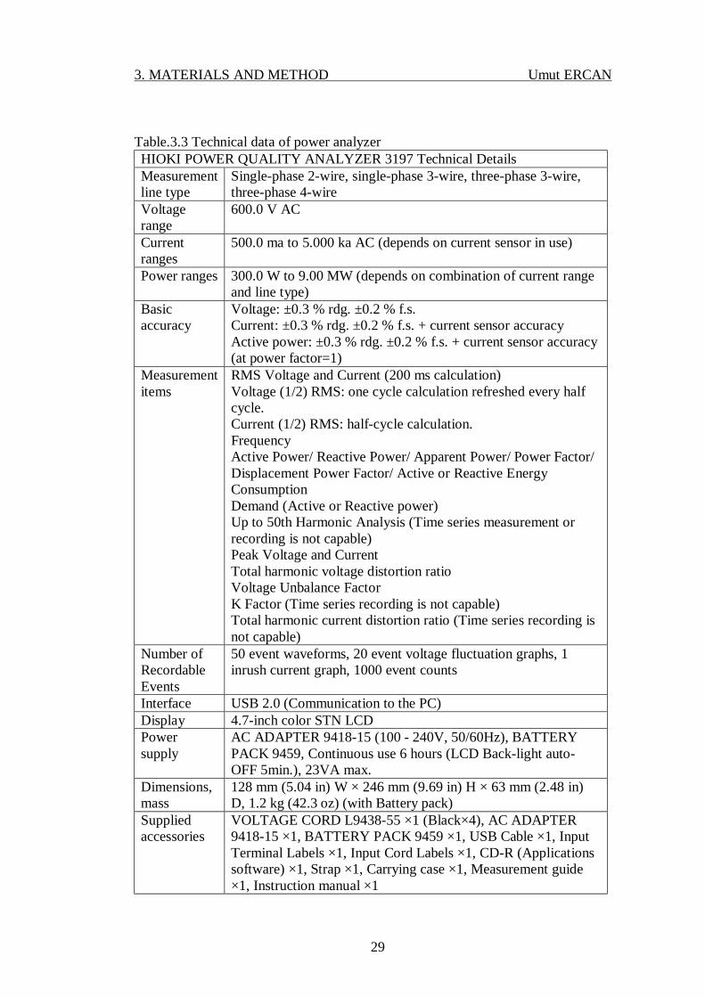
3.3.2.1. Power Analyzer
Power analyzer instrument utilized during the experiment is Hioki Power
Quality Analyzer 3197 for measuring, monitoring, recording and analyzing the
power quality of AC power systems, Fig. 3.11. Technical data has been given in
Table 3.3.
Figure 3.11 Power quality analyzer
3. MATERIALS AND METHOD Umut ERCAN
29
Table.3.3 Technical data of power analyzer HIOKI POWER QUALITY ANALYZER 3197 Technical Details Measurement line type
Single-phase 2-wire, single-phase 3-wire, three-phase 3-wire, three-phase 4-wire
Voltage range
600.0 V AC
Current ranges
500.0 ma to 5.000 ka AC (depends on current sensor in use)
Power ranges 300.0 W to 9.00 MW (depends on combination of current range and line type)
Basic accuracy
Voltage: ±0.3 % rdg. ±0.2 % f.s. Current: ±0.3 % rdg. ±0.2 % f.s. + current sensor accuracy Active power: ±0.3 % rdg. ±0.2 % f.s. + current sensor accuracy (at power factor=1)
Measurement items
RMS Voltage and Current (200 ms calculation) Voltage (1/2) RMS: one cycle calculation refreshed every half cycle. Current (1/2) RMS: half-cycle calculation. Frequency Active Power/ Reactive Power/ Apparent Power/ Power Factor/ Displacement Power Factor/ Active or Reactive Energy Consumption Demand (Active or Reactive power) Up to 50th Harmonic Analysis (Time series measurement or recording is not capable) Peak Voltage and Current Total harmonic voltage distortion ratio Voltage Unbalance Factor K Factor (Time series recording is not capable) Total harmonic current distortion ratio (Time series recording is not capable)
Number of Recordable Events
50 event waveforms, 20 event voltage fluctuation graphs, 1 inrush current graph, 1000 event counts
Interface USB 2.0 (Communication to the PC) Display 4.7-inch color STN LCD Power supply
AC ADAPTER 9418-15 (100 - 240V, 50/60Hz), BATTERY PACK 9459, Continuous use 6 hours (LCD Back-light auto-OFF 5min.), 23VA max.
Dimensions, mass
128 mm (5.04 in) W × 246 mm (9.69 in) H × 63 mm (2.48 in) D, 1.2 kg (42.3 oz) (with Battery pack)
Supplied accessories
VOLTAGE CORD L9438-55 ×1 (Black×4), AC ADAPTER 9418-15 ×1, BATTERY PACK 9459 ×1, USB Cable ×1, Input Terminal Labels ×1, Input Cord Labels ×1, CD-R (Applications software) ×1, Strap ×1, Carrying case ×1, Measurement guide ×1, Instruction manual ×1

3. MATERIALS AND METHOD Umut ERCAN
30
3.3.2.2. Torque Meter
In order to measure the torque on the cylinder shaft, Checkline DIW-75
digital torque meter has been used in experiments. Basic reasons for selecting this
device are its convenience in connection with the shaft, suitable interval of torque
measurement, digital display, and transfer of measured torque value to a computer.
Technical data of the selected torque meter have been presented in Table 3.4.
Table.3.4 Technical data of torque meter Torque meter technical data Measurement: 0.30-75 Nm (55 lb-ft) Accuracy ±0.5%, ±1 LSD Sampling Frequency 100 Hz (100 samples/sec) Display Update Rate 5 Hz (5 times/sec) USB Output 180 data/sec Memory 400 data memory for recall or for SPC download Drive 3/8"
Figure 3.12 Torque meter
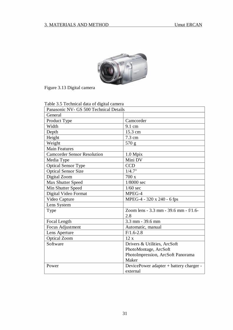
3.3.2.3. Camera
A digital camera has been used in finding the angle of equilibrium and, in
observing and recording the flow rate pattern. Technical data associated with digital
camera are shown in Table 3.5.
3. MATERIALS AND METHOD Umut ERCAN
31
Figure 3.13 Digital camera
Table 3.5 Technical data of digital camera Panasonic NV- GS 500 Technical Details General Product Type Camcorder Width 9.1 cm Depth 15.3 cm Height 7.3 cm Weight 570 g Main Features Camcorder Sensor Resolution 1.0 Mpix Media Type Mini DV Optical Sensor Type CCD Optical Sensor Size 1/4.7" Digital Zoom 700 x Max Shutter Speed 1/8000 sec Min Shutter Speed 1/60 sec Digital Video Format MPEG-4 Video Capture MPEG-4 - 320 x 240 - 6 fps Lens System Type Zoom lens - 3.3 mm - 39.6 mm - f/1.6-
2.8 Focal Length 3.3 mm - 39.6 mm Focus Adjustment Automatic, manual Lens Aperture F/1.6-2.8 Optical Zoom 12 x Software Drivers & Utilities, ArcSoft
PhotoMontage, ArcSoft PhotoImpression, ArcSoft Panorama Maker
Power DevicePower adapter + battery charger - external
3. MATERIALS AND METHOD Umut ERCAN
32
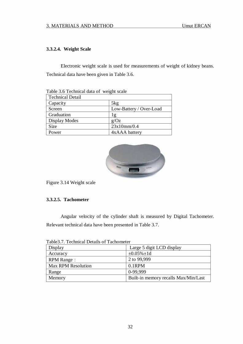
3.3.2.4. Weight Scale
Electronic weight scale is used for measurements of weight of kidney beans.
Technical data have been given in Table 3.6.
Table 3.6 Technical data of weight scale Technical Detail Capacity 5kg Screen Low-Battery / Over-Load Graduation 1g Display Modes g/Oz Size 23x10mm/0.4 Power 4xAAA battery
Figure 3.14 Weight scale
3.3.2.5. Tachometer
Angular velocity of the cylinder shaft is measured by Digital Tachometer.
Relevant technical data have been presented in Table 3.7.
Table3.7. Technical Details of Tachometer Display Large 5 digit LCD display Accuracy ±0.05%±1d RPM Range: 2 to 99,999 Max RPM Resolution 0.1RPM Range 0-99,999 Memory Built-in memory recalls Max/Min/Last

3. MATERIALS AND METHOD Umut ERCAN
33
Figure 3.15 Digital tachometer
3.3.2.6. Meter
Meter is used for measuring feeder opening and in the manufacturing of some
parts of the system such as shaft - torque meter connection, and speed adjustment
operation. Division is 1 mm.
Figure 3.16 Meter
3.3.2.7. Chronometer
Electronic chronometer with digital display is used for measuring time for the
flow from the feeder to the cylinder. Resolution and accuracies are both 1 second.
Figure 3.17 Chronometer

3. MATERIALS AND METHOD Umut ERCAN
34
3.3.2.8. Erlenmeyer Glass
In order to measure volume of the granular material Erlenmeyer glass is used.
Division is 10 ml.
3.3.2.9.Protractor
Protractor is used for measuring angles in the in determining coefficient
friction Resolution is 1°.
3.3.2.10. Laptop
Laptop is used in the experiments to collect all the digital data coming from
digital camera, digital torque meter, and power analyzer.
Technical data associated with laptop have been shown in Table 3.8.
Table 3.8 Technical detail of laptop
Processor Intel Core 2 Duo P7350 (2,00 GHz, 1066 MHz, 3 MB)
Graphic ATI Mobility Radeon HD 4650
Storage 320 gigabyte
Display 15.6”
Operating System Windows 7
3.4. Experiments
3.4.1. Equilibrium Angle
First, grid systems the lines of which are parallel and perpendicular to the
shaft axis are drawn on the internal surface of the sieve. At the same time circular
grid line in the middle of the cylinder perpendicular to the shaft axis is also marked
on the shaft. By means of a digital camera basically positioned along the main axis of

3. MATERIALS AND METHOD Umut ERCAN
35
the sieve shaft, camera shots are taken while the machine is operated. Based on the
digital camera recordings belonging to a certain cross section of the cylinder,
equilibrium angle is measured.
The experiments are also repeated for different feeder gate opening heights
varying from 2.0 cm to 3.5 cm with equal 0.5 cm intervals.
3.4.2. Experiment on Bulk Density
The purpose of this experiment is to provide the value of the bulk density
needed in the mathematical model and to find the mass flow rate. The following
steps are implemented for that purpose: Firstly, the masses of bulk material of big-
size and of small-size are measured by means of weight scale and recorded. The bulk
material is placed inside the Erlenmeyer glass with volumetric division. Then they
are shaken for some time until they are settled with no excessive space between the
beans. Their volumes are read off the glass and recorded. Masses are divided by
volume values to calculate bulk density.
Experiments are repeated by taking into account different mixing ratios (the
ratio of small size material to total mass). In this way, the densities of the mixture are
found against different mixing ratios.
3.4.3. Experiment for Coefficient of Friction
In order to determine friction coefficient required in the calculations, a plate
made out of material similar to that of the sieve is prepared in the rectangular form.
Kidney bean is placed on this plate. By keeping one end of the plate fixed on the
ground, the other end is raised gradually giving angular orientation to the plate.
Tilting the plate continues until the beans starts sliding on the surface. Then the
inclination angle is measured by means of protractor. Tangent of the angle becomes
the coefficient of friction.

3. MATERIALS AND METHOD Umut ERCAN
36
3.4.4. Efficiency and Flow Rate Experiments
With the purpose of determining performance parameters of the sieve such as
efficiency and flow rate, the following steps are executed. By mixing the kidney
beans in various proportions with respect to sizes, a specimen of 10 kg mixture is
obtained. The mixture is poured into the container while the feeder gate is closed. As
soon as the switch of the machine is turned on, chronometer is operated until the
feeder box is emptied and the time elapsed for emptying the feeder box is measured
and recorded. After the separation process in the cylinder, the amounts of beans that
have fallen into small-size and big-size boxes are measured, analyzed and recorded.
The experiments are repeated for the proportions of the small size in the lot
varying between 10 - 90 % with equal intervals of 10 %.
The experiments are also repeated for different feeder gate opening heights
varying from 2.0 cm to 3.5 cm with equal 0.5 cm intervals.
3.4.5. Experiment on Torque
Torque measurement is needed not only to determine the torque required to
the drive the cylinder determine but also to determine the mechanical power
consumed by the different parts of the system including material processed and
friction due to brushing operation, on the basis of constant angular velocity of the
rotating cylinder.
During all the torque measurement the connection between the driving unit
(electrical motor and reducer) and accompanying transmission part (belt-drives) is
cut off. Instead cylinder shaft is rotated manually through the torque wrench. An
intermediate piece for coupling the shaft of sieve with the probe of the torque meter
is designed and manufactured.
The experiments are carried out in such a way that torque measurement is
taken under two different conditions whereby processed material are on the system
together with the brushes, the other includes only brushes (without material) while
the cylinder is rotating.

3. MATERIALS AND METHOD Umut ERCAN
37
In measuring the torque values, the circumference of the cylinder is divided
into twelve parts with equal spacing. This amounts to torque value corresponding to
every 30 - degree rotation of the cylinder. The measurements at each marked point of
the cylinder are repeated 4 times.
The experiments are repeated at different opening heights of the feeder gate.
All the results are collected in a computer.
3.4.6. Experiment on Power
To measure total energy consumed by the whole system including electrical and
mechanical parts such as electrical motor, reducer, bearings, pulley system, spatial
cam mechanism, brushes, experiments are carried out using power analyzer by
operating the system with or without any material inside with brushes attached and
also unloaded system without brushes.
The experiments are repeated at different opening heights of the feeder gate.
All the results are collected in a computer.
3.4.7. Experiment on Energy
Using power analyzer energy under loaded and unloaded conditions with and
without brush are measured and recorded. By taking difference between the energy
values when there is load and no load in the system and also when there are brush
and no brushes, energy only due to processed material and also energy consumed
only by brushes are calculated.
Calculations are repeated for each feeder gate height.

4. RESULTS AND DISCUSSION Umut ERCAN
38
4. RESULTS AND DISCUSSION
In this section, results of bulk density, equilibrium angle, coefficient of
friction, efficiency, mass flow rate, torque and energy consumption experiments will
be presented in graphical and/or tabular forms.
4.1. Equilibrium Angle
Following the procedure of section 3.1.5.3., exemplary values of the
equilibrium angle (β) as calculated according to formula (3.51.), are tabulated in
Table 4.1. Its graphical form is displayed in Fig. 4.1.
Table 4.1 Number of layer n=1
Number of layer (n)
Equilibrium Angle (β ) (°)
Equilibrium Angle (β) (rad) Result
1 0 0 0 1 1 0,017453 -0,00098 1 10 0,174533 -0,07401 1 20 0,349066 -0,18775 1 30 0,523599 -0,17726 1 31 0,541052 -0,16317 1 32 0,558505 -0,14607 1 33 0,575959 -0,12582 1 34 0,593412 -0,10226 1 35 0,610865 -0,07525 1 36 0,628319 -0,04464 1 37 0,645772 -0,01028 1 38 0,663225 0,027975 1 39 0,680678 0,070267 1 40 0,698132 0,116737 1 50 0,872665 0,840781 1 60 1,047198 2,121002 1 70 1,22173 4,056361 1 80 1,396263 6,712996 1 90 1,570796 10,11996

4. RESULTS AND DISCUSSION Umut ERCAN
39
Figure 4.1 Theoretical equilibrium angle
Theoretical equilibrium angles corresponding to different numbers of layers
(n) have been collected in Table 4.2. The graphical form of Table 4.2 is shown in
Fig.4.2 in which abscissa is number of layer (n) and the ordinate is equilibrium angle
(β). By non - linear regression the expression between equilibrium angle and number
of layer is found to be:
β = -0,0139n2 + 0,1211n + 0,5457 (4.70.)
It is observed that equilibrium angle increases with increasing number of layers.
Furthermore, the slope of the curve in Fig.4.2 decreases with increasing number of
layers. This point is supported by the derivative expression of equation (4.70.), given
as follows:
dβ/dn = -0,0278n + 0,1211 (4.71.)
If the slope of angle (β) is plotted against number of layers (n), the resulting curve is
seen in Fig. 4.3. From Fig. 4.3 it is deduced that slope goes to zero when n is
4,339069. In this case equilibrium angle has an asymptotic value as implied by Fig.
4.3.
-2
0
2
4
6
8
10
12
0 10 20 30 40 50 60 70 80 90
Root
s
Equlilibrium Angle

4. RESULTS AND DISCUSSION Umut ERCAN
40
Table.4.2 Theoretical equilibrium angle against - number of layer Number of Layer 1 1,25 1,5 1,75 2 2,25 2,5 2,75 3 3,5 Theoretical Equilibrium Angle 37,28 38,73 39,97 41,05 41,98 42,83 43,56 44,22 44,82 45,86
Figure 4.2 Theoretical equilibrium angle vs Number of layer
Table. 4.3. Number of layer- result of equation (4.71.) root 1 1,25 1,5 1,75 2 2,25 2,5 2,75 3 3,5 4 4,25 4,32 4,33 4,33
9069
result 5,34
72
4,94
685
4,54
65
4,14
615
3,74
58
3,34
545
2,94
51
2,54
475
2,14
44
1,34
37
0,54
3
0,14
265
0,03
0552
0,01
4538
1,49
E-05
y = -0,8007x2 + 6,9486x + 31,256R² = 0,9992
05
101520253035404550
0 0,5 1 1,5 2 2,5 3 3,5 4
beta
ang
le
number of layer

4. RESULTS AND DISCUSSION Umut ERCAN
41
Figure 4.3 dβ/dn vs number of layer
On the other hand, the camera shots taken during the experiments carried out
according to section 3.4.1 are displayed in Figures 4.4 - 4.7 corresponding to feeder
gate heights of 2cm - 3.5cm with 0.5 cm intervals, respectively. By using image
processing software (Corel Draw X5) equilibrium angles are measured from Fig. 4.4
- 4.7. The measurement results are collected in Table 4.4. When the values in Table
4.4 are plotted on a pair of axis the resulting curve turns out to be the one shown in
Fig. 4.8. By non- linear regression the equation of the curve is the following:
0
1
2
3
4
5
6
1 1,5 2 2,5 3 3,5 4 4,5
dβ/d
n
number of layer

4. RESULTS AND DISCUSSION Umut ERCAN
42
Figure 4.4 Equilibrium Angle for 2cm feeder gate height
Figure 4.5 Equilibrium angle for 2.5cm feeder gate height

4. RESULTS AND DISCUSSION Umut ERCAN
43
Figure 4.6 Equilibrium angle for 3 cm feeder gate height
Figure 4.7 Equilibrium angle for 3.5 cm feeder gate height

4. RESULTS AND DISCUSSION Umut ERCAN
44
β = -0,0139x2 + 0,1211x + 0,5457 (4.72.)
where x represents the opening height of the feeder gate in cm.
Table.4.4. Experimental values of equilibrium angles
Feeder Gate
Heights (cm)
2.0 2.5 3.0 3.5
Equilibrium
Angles (°)
37.58 38.96 40.26 43.19
Equilibrium
Angles (rad)
0.655895 0.67998 0.70267 0.753808
Figure 4.8 Equilibirum angle vs feeder gate heights
By comparison of experimental values with the theoretical values semi-
empirical values of number of layers are determined and the results are tabulated in
Table 4.5. When the values in Table 4.5 are plotted on a pair of axis the resulting
curve turns out to be the one shown in Fig. 4.9. As feeder gate height is increased,
number of layer also increases.
37
38
39
40
41
42
43
44
2 2,5 3 3,5
Equi
libriu
m A
ngle
feeder gate heights
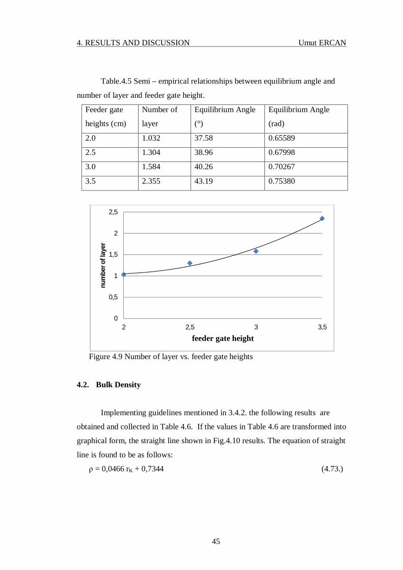
4. RESULTS AND DISCUSSION Umut ERCAN
45
Table.4.5 Semi – empirical relationships between equilibrium angle and
number of layer and feeder gate height.
Feeder gate
heights (cm)
Number of
layer
Equilibrium Angle
(°)
Equilibrium Angle
(rad)
2.0 1.032 37.58 0.65589
2.5 1.304 38.96 0.67998
3.0 1.584 40.26 0.70267
3.5 2.355 43.19 0.75380
Figure 4.9 Number of layer vs. feeder gate heights
4.2. Bulk Density
Implementing guidelines mentioned in 3.4.2. the following results are
obtained and collected in Table 4.6. If the values in Table 4.6 are transformed into
graphical form, the straight line shown in Fig.4.10 results. The equation of straight
line is found to be as follows:
ρ = 0,0466 rK + 0,7344 (4.73.)
0
0,5
1
1,5
2
2,5
2 2,5 3 3,5
num
ber o
f lay
er
feeder gate height

4. RESULTS AND DISCUSSION Umut ERCAN
46
Table.4.6 Mixture Bulk Density Big - Size Kidney Beans Mass (gr)
Small - Size Kidney Beans Mass (gr)
Mixture Volume(ml)
Small - Size Ratio(rk)
Mixture Bulk Density
0 500 640 1 0,78125 125 375 650 0,75 0,76923 250 250 660 0,5 0,75757 375 125 670 0,25 0,74626 500 0 680 0 0,73529
Figure 4.10 Measured bulk density vs small size ratio
4.3. Coefficient of Friction
Coefficient of friction experiments explained in section 3.4.3 have been
applied and the resulting values are tabulated in Table 4.7.
Table.4.7 Coefficient of friction values
Experiment Number
1 2 3 Average Standard Deviation
Results 0,3249 0,3315 0,3176 0,3246 0,005677
y = 0,0466x + 0,7344R² = 0,9998
0,740,745
0,750,755
0,760,765
0,770,775
0,780,785
0 0,2 0,4 0,6 0,8 1 1,2
Bulk
Den
sity
Small Size Ratio

4. RESULTS AND DISCUSSION Umut ERCAN
47
4.4. Efficiency and Flow Rate
Efficiency and flow rate experiments described in section 3.4.4 have been
carried out to yield results tabulated according to the specific feeder gate heights in
Table 4.8 to Table 4.11. Efficiency values contain in Tables 4.8 - Table 4.11have
been plotted against small- size ratio as shown in Fig. 4.11.
Table.4.8 Experiment result for 2 cm feeder height Exp. No.
input Dropped into box Time (s)
Mass Flow rate (kg/s)
Efficiency (%) Big size
Kidney beans (g)
Small size Kidney beans (g)
Big size Kidney beans (g)
Small size Kidney beans (g)
1 9000 1000 9007 993 87,13 0,114771
99,86005
2 8000 2000 8014 1986 83,6 0,119617
99,72024
3 7000 3000 7018 2985 80,75 0,123839
99,67046
4 6000 4000 6018 3977 74,96 0,133404
99,59054
5 5000 5000 5030 4963 70,08 0,142694
99,33179
6 4000 6000 4049 5951 64,03 0,156177
99,02593
7 3000 7000 3062 6938 59,34 0,16852 98,77255 8 2000 8000 2080 7920 52,96 0,18882
2 98,43077
9 1000 9000 1070 8930 49,12 0,203583
98,64579

4. RESULTS AND DISCUSSION Umut ERCAN
48
Table.4.9 Experiment result for 2.5 cm feeder height Exp. No.
input Dropped into box Time(s) Mass Flow rate (kg/s)
Efficiency (%) Big Kidney
beans (g) Small Kidney beans (g)
Big Kidney beans (g)
Small Kidney beans (g)
1 9000 1000 9015 985 42,39 0,235905 99,70025 2 8000 2000 8019 1981 41,8 0,239234 99,62045 3 7000 3000 7035 2965 38,47 0,259943 99,30174 4 6000 4000 6049 3951 36,81 0,271665 99,02397 5 5000 5000 5058 4942 33,81 0,29577 98,84665 6 4000 6000 4097 5903 32,92 0,303767 98,08297 7 3000 7000 3097 6903 32,22 0,310366 98,09038 8 2000 8000 2098 7902 31,12 0,321337 98,08578 9 1000 9000 1094 8906 30,78 0,324886 98,20077
Table.4.10 Experiment result for 3 cm feeder height Exp. No.
input Dropped into box Time(s) Mass Flow rate (kg/s)
Efficiency (%) Big Kidney
beans (g) Small Kidney beans (g)
Big Kidney beans (g)
Small Kidney beans (g)
1 9000 1000 9031 969 31,21 0,32041 99,38106 2 8000 2000 8079 1921 30,03 0,333 98,42772 3 7000 3000 7085 2915 29,75 0,336134 98,3102 4 6000 4000 6101 3899 28,34 0,352858 97,99672 5 5000 5000 5113 4887 27,91 0,358295 97,76497 6 4000 6000 4146 5854 25,96 0,385208 97,13141 7 3000 7000 3163 6837 23,31 0,429 96,824 8 2000 8000 2175 7825 21,13 0,473261 96,6408 9 1000 9000 1153 8847 20,94 0,477555 97,14303

4. RESULTS AND DISCUSSION Umut ERCAN
49
Table.4.11 Experiment result for 3.5 cm feeder height Exp. No.
input Dropped into box Time(s) Mass Flow rate (kg/s)
Efficiency (%) Big Kidney
beans (g) Small Kidney beans (g)
Big Kidney beans (g)
Small Kidney beans (g)
1 9000 1000 9098 902 21,89 0,45683 98,05056 2 8000 2000 8115 1885 21,56 0,463822 97,7163 3 7000 3000 7116 2884 20,01 0,49975 97,69891 4 6000 4000 6150 3850 19,11 0,523286 97,03659 5 5000 5000 5173 4827 18,94 0,527983 96,59786 6 4000 6000 4239 5761 18,21 0,549149 95,35475 7 3000 7000 3253 6747 17,79 0,562114 95,13677 8 2000 8000 2257 7743 15,97 0,626174 95,15264 9 1000 9000 1265 8735 15,44 0,647668 95,25514
Figure 4.11 Efficiency vs small - size ratio
y = 7,5751x3 - 11,978x2 + 3,5503x + 99,543R² = 0,9703
y = 11,756x3 - 15,656x2 + 3,1237x + 99,523R² = 0,9729
y = 6,9733x3 - 6,715x2 - 2,3629x + 99,474R² = 0,9464
y = 22,941x3 - 32,534x2 + 8,3417x + 97,414R² = 0,9772
94
95
96
97
98
99
100
0 0,1 0,2 0,3 0,4 0,5 0,6 0,7 0,8 0,9
Effic
ienc
y (%
)
Small Size Ratio
2 cm 2.5 cm 3 cm 3.5 cm

4. RESULTS AND DISCUSSION Umut ERCAN
50
From Fig. 4.11 efficiency values are observed to decrease against increasing
small- size ratio up to a certain point and then have appeared to stabilize. When the
feeder gate height is increased efficiencies have decreasing tendencies.
Figure 4.12 Mass flow rate vs small - size ratio
Upon evaluating the mass flow rate values against small- size kidney bean
composition the curve shown in Fig. 4.12 results. As the small – size ratio increases,
mass flow rate increases. When the opening height of the feeder gate is increased
flow rate increases too.
0
0,1
0,2
0,3
0,4
0,5
0,6
0,7
0 0,1 0,2 0,3 0,4 0,5 0,6 0,7 0,8 0,9
Mas
s Flo
wra
te (k
g/s)
Small - Size Ratio
2 cm
2.5 cm
3 cm
3.5 cm

4. RESULTS AND DISCUSSION Umut ERCAN
51
Figure 4.13 Efficiency vs mass flow rate
Based on the efficiency and mass flow rate values from Tables 4.8 to Table
4.11 efficiency vs mass flow rate curve has been drawn in Fig.4.13. Efficiency is
seen to be influenced by the mass flow rate negatively meaning that as the gate
height is raised mass flow rate becomes larger leading to decreasing efficiencies.
Although efficiency shows decreasing tendencies with increasing mass flow rate,
after a certain point they appear to be constant. The efficiency never drops below 95
% within the operating conditions.
4.5. Torque
Torque experiment has been explained in section 3.4.5. Torque values
collected from the experiments without and with brush are collected in Table 4.12
and Table 4.13, respectively. It is observed that the average torque values
corresponding to one revolution of the cylinder without and with brush are
3,058654Nm and 4, 935192Nm respectively. From these values it is observed that
brushes require approximately 38 % of the driving torque applied on the machine,
when there are no kidney beans in the cylinder.
94
95
96
97
98
99
100
0 0,1 0,2 0,3 0,4 0,5 0,6 0,7 0,8
Effic
ienc
y (%
)
Mass Flowrate (kg/s)
2 cm
2.5 cm
3 cm
3.5 cm
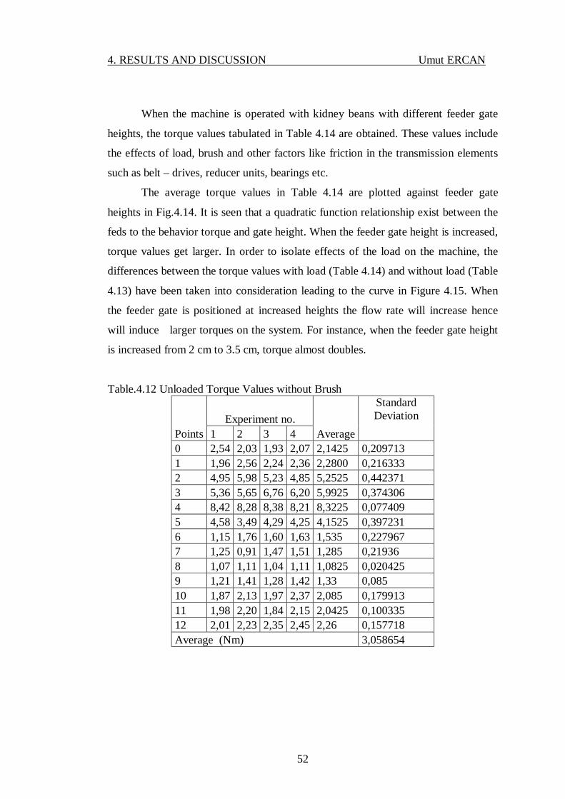
4. RESULTS AND DISCUSSION Umut ERCAN
52
When the machine is operated with kidney beans with different feeder gate
heights, the torque values tabulated in Table 4.14 are obtained. These values include
the effects of load, brush and other factors like friction in the transmission elements
such as belt – drives, reducer units, bearings etc.
The average torque values in Table 4.14 are plotted against feeder gate
heights in Fig.4.14. It is seen that a quadratic function relationship exist between the
feds to the behavior torque and gate height. When the feeder gate height is increased,
torque values get larger. In order to isolate effects of the load on the machine, the
differences between the torque values with load (Table 4.14) and without load (Table
4.13) have been taken into consideration leading to the curve in Figure 4.15. When
the feeder gate is positioned at increased heights the flow rate will increase hence
will induce larger torques on the system. For instance, when the feeder gate height
is increased from 2 cm to 3.5 cm, torque almost doubles.
Table.4.12 Unloaded Torque Values without Brush
Points Experiment no.
Average
Standard Deviation
1 2 3 4 0 2,54 2,03 1,93 2,07 2,1425 0,209713 1 1,96 2,56 2,24 2,36 2,2800 0,216333 2 4,95 5,98 5,23 4,85 5,2525 0,442371 3 5,36 5,65 6,76 6,20 5,9925 0,374306 4 8,42 8,28 8,38 8,21 8,3225 0,077409 5 4,58 3,49 4,29 4,25 4,1525 0,397231 6 1,15 1,76 1,60 1,63 1,535 0,227967 7 1,25 0,91 1,47 1,51 1,285 0,21936 8 1,07 1,11 1,04 1,11 1,0825 0,020425 9 1,21 1,41 1,28 1,42 1,33 0,085 10 1,87 2,13 1,97 2,37 2,085 0,179913 11 1,98 2,20 1,84 2,15 2,0425 0,100335 12 2,01 2,23 2,35 2,45 2,26 0,157718 Average (Nm) 3,058654

4. RESULTS AND DISCUSSION Umut ERCAN
53
Table 4.13 Unloaded Torque Values with Brush
Points Measurement Number
Average
Standard Deviation
1 2 3 4 0 5,24 5,76 5,48 4,95 5,3575 0,292348 1 1,99 2,32 2,03 1,87 2,0525 0,164901 2 6,36 6,21 6,15 6,38 6,275 0,074958 3 5,91 5,42 5,1 4,61 5,26 0,46653 4 8,63 8,58 9,32 9,48 9,0025 0,369212 5 5,46 5,18 5,26 5,51 5,3525 0,128568 6 9,42 9,8 9,23 9,64 9,5225 0,159153 7 1,49 1,61 1,02 1,07 1,2975 0,21591 8 1,26 1,12 1,27 1,04 1,1725 0,083619 9 4,91 4,76 4,83 4,23 4,6825 0,256183 10 3,46 3,11 3,06 3,36 3,2475 0,138491 11 5,67 5,99 5,5 5,72 5,72 0,137295 12 5,04 5,54 5,14 5,14 5,215 0,188331 Average (Nm) 4, 935192
Table.4.14 Loaded Torque Values With Brush
Points Feeder Gate Heights
2 cm 2.5 cm 3 cm 3.5 cm 0 7,10 10,46 11,50 13,10 1 11,16 12,35 14,40 15,32 2 9,25 14,80 14,01 15,10 3 13,75 11,85 20,80 19,50 4 12,10 14,60 22,30 18,79 5 15,40 15,43 22,60 23,10 6 15,80 16,80 24,30 30,30 7 8,80 11,50 16,05 27,60 8 6,02 10,05 12,90 20,80 9 5,90 10,30 12,50 16,70 10 8,20 8,26 13,30 15,15 11 8,80 10,5 11,40 16,20 12 8,05 9,90 13,60 17,50 Average (Nm) 10,02 12,06 16,12 19,16

4. RESULTS AND DISCUSSION Umut ERCAN
54
Figure 4.14 Experimental torque values vs feeder gate heights
Figure 4.15 Experimental torque due to load vs. feeder gate height
Theoretical torque values have been calculated according to formula (3.55.). By
taking into consideration the experimental conditions summarized in Table 4.15,
theoretical torque values vs. number of layer are calculated and collected in Table
4.16. Its graphical form is displayed in Fig.4.16. In view of the results summarized
in Table 13 the torque values versus feeder gate heights are calculated and tabulated
in Table 4.17. As can be seen from Fig. 4.17, as the feeder gate height increases,
y = 1x2 + 0,796x + 4,276R² = 0,9908
0
5
10
15
20
25
2 2,5 3 3,5
Torq
ue V
alue
s (N
m)
Feeder gate heights (cm)
y = 1,0023x2 + 0,785x - 0,6419R² = 0,9907
0
2
4
6
8
10
12
14
16
2 2,5 3 3,5
Torq
ue d
ue to
load
(Nm
)
Feeder gate heights (cm)

4. RESULTS AND DISCUSSION Umut ERCAN
55
torque values also increase. From Fig.4.18 it is clearly observed that theoretical and
experimental torque behavior under similar operating conditions agree with each
other.
Table 4.15 Values of Parameters in Theoretical Torque Calculation Bean thickness (e)
Gravitation acceleration (g)
Radius of cylinder (r )
Bulk Density (ρ)
Angular Speed of Cylinder (w)
6 mm 9,80665 m/s2 0,318 m 744,69 kg/m3 1,047 rad/s
Table 4.16. Theoretical Torque Values Number of Layer (n) Beta Angle (°) Beta Angle (rad) Torque (T) (Nm/m) 1 37,28 0,650328889 9,044347 1,25 38,73 0,675623333 11,52778 1,5 39,97 0,697254444 13,88164 1,75 41,05 0,716094444 16,04435 2 41,988 0,732457333 17,95364 2,25 42,83 0,747145556 19,58566 2,5 43,563 0,759932333 20,87996 2,75 44,226 0,771498 21,83051 3 44,824 0,781929778 22,40923 3,25 45,37 0,791454444 9,415314 3,5 45,86 0,800002222 12,01771
Table 4.17 Experimental and Theoretical Torque Values due to Load Experiment Torque Values (Nm)
Theoretical Torque Value (Nm)
Feeder gate heights(cm)
Number of layer
5,084808 4,480122 2 1,032 7,124808 7,08252 2,5 1,304 11,18481 9,635365 3 1,584 14,22481 15,27262 3,5 2,355

4. RESULTS AND DISCUSSION Umut ERCAN
56
Figure 4.16 Theoretical torque vs. number of layer
Figure 4.17 Theoretical torque values vs. feeder gate heights
y = -2,228x2 + 15,706x - 4,5537R² = 0,9996
0
5
10
15
20
25
1 1,25 1,5 1,75 2 2,25 2,5 2,75 3 3,25 3,5
Theo
retic
al T
orqu
e(N
m)
Number of layer
y = 3,0349x2 - 9,7057x + 16,844R² = 0,9923
0
5
10
15
20
25
2 2,5 3 3,5
Theo
retic
al to
rque
val
ues (
Nm
)
feeder gate height (cm)

4. RESULTS AND DISCUSSION Umut ERCAN
57
Figure 4.18 Experimental and theoretical torque values due to load vs. feeder gate heights
4.6. Power
Power experiments have been explained in section 3.4.6. Unloaded power
measurements over 91- second time span are recorded and displayed in Fig.4.19.
When the power values with brush are subtracted from those without brush, power
consumption due to only brush effect is deduced as shown in Fig. 4.20. Under
unloaded conditions average brush consumption over the given time span turns out to
be 9,03 W.
Under normal operating conditions loaded experimental power values are
recorded against time and the resulting curves are shown in Fig 4.21. When the
differences between the loaded and unloaded power measurements for different gate
heights are computed, results exhibited in Table 4.18 are obtained. Experimental
power values due to load, corresponding to different feeder gate heights have been
plotted in Fig.4.22. From Fig.4.22 average and standard deviation values of
experimental power corresponding to different feeder gate heights have been
computed and tabulated in Table 4.18. Most of the time standard deviation is less
y = 1x2 + 0,796x - 0,6592R² = 0,9908
y = 3,0349x2 - 9,7056x + 11,909R² = 0,9923
0
2
4
6
8
10
12
14
16
18
2 2,5 3 3,5
Torq
ue v
alue
s (N
m)
feeder gate height (cm)
experimental
theoretical

4. RESULTS AND DISCUSSION Umut ERCAN
58
than 1 %. By plotting average experimental power against feeder gate heights the
curve shown in Fig. 4.23 is obtained. It’s observed that from Fig.4.23 there is a
quadratic relationship between the power values and feeder gate heights.
Theoretical power values have been calculated from equation (3.55.) and
(3.56.) under the experimental conditions shown in Table 4.15. Then the resulting
theoretical power values versus different feeder gate heights are plotted in Fig.4.24
by making use of Table 4.15. As can be seen in Table 4.19 it is observed that
theoretical and experimental power behaviors under similar conditions are in
harmony with each other.
Figure 4.19 Unloaded experimental power with and without brush vs. time
Figure 4.20 Power values due to brush vs time
335
340
345
350
355
360
365
370
0 20 40 60 80 100
Pow
er (w
)
Time (s)
With Brush
Without Brush
02468
1012141618
0 20 40 60 80 100
Pow
er v
alue
s due
to b
rush
(w)
Time (s)

4. RESULTS AND DISCUSSION Umut ERCAN
59
Figure 4.21 Loaded experimental power vs. time for different feeder gate heights
Figure 4.22 Power due to load vs time
Table 4.18 Experimental Power (Loaded) for Different Feeder Gate Heights Feeder Gate Height
2 cm 2,5 cm 3 cm 3,5 cm
Average Power 364,2283 W 370,5543 W 374,5217 W 379,1413W Standard Deviation 2,801504 4,312935 3,303273 3,621006
350
355
360
365
370
375
380
385
390
0 20 40 60 80 100
Expe
rimen
tal P
ower
val
ues (
w)
time (s)
2 cm
2,5 cm
3 cm
3,5 cm
05
10152025303540
4550
0 20 40 60 80 100
Pow
er d
ue to
load
(w)
Time (s)
2 cm
2,5 cm
3 cm
3,5 cm
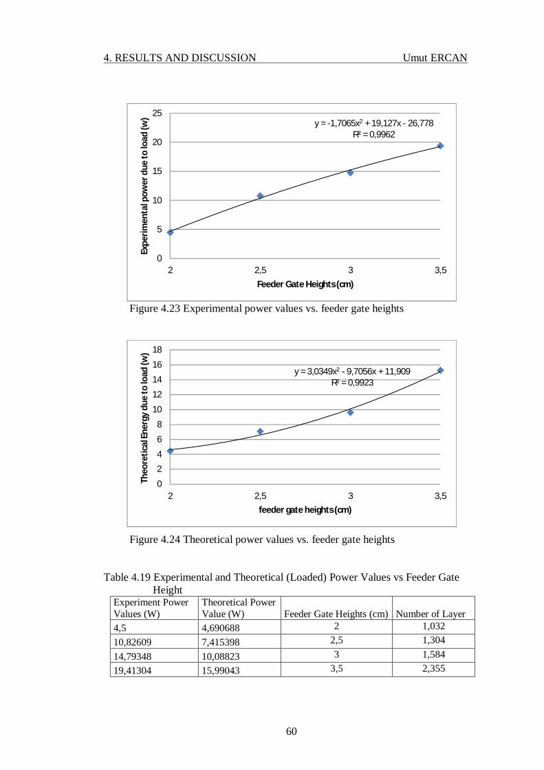
4. RESULTS AND DISCUSSION Umut ERCAN
60
Figure 4.23 Experimental power values vs. feeder gate heights
Figure 4.24 Theoretical power values vs. feeder gate heights
Table 4.19 Experimental and Theoretical (Loaded) Power Values vs Feeder Gate Height
Experiment Power Values (W)
Theoretical Power Value (W) Feeder Gate Heights (cm) Number of Layer
4,5 4,690688 2 1,032 10,82609 7,415398 2,5 1,304 14,79348 10,08823 3 1,584 19,41304 15,99043 3,5 2,355
y = -1,7065x2 + 19,127x - 26,778R² = 0,9962
0
5
10
15
20
25
2 2,5 3 3,5
Expe
rimen
tal p
ower
due
to lo
ad (w
)
Feeder Gate Heights (cm)
y = 3,0349x2 - 9,7056x + 11,909R² = 0,9923
0
2
4
6
8
10
12
14
16
18
2 2,5 3 3,5
Theo
retic
al En
ergy
due
to lo
ad (w
)
feeder gate heights (cm)
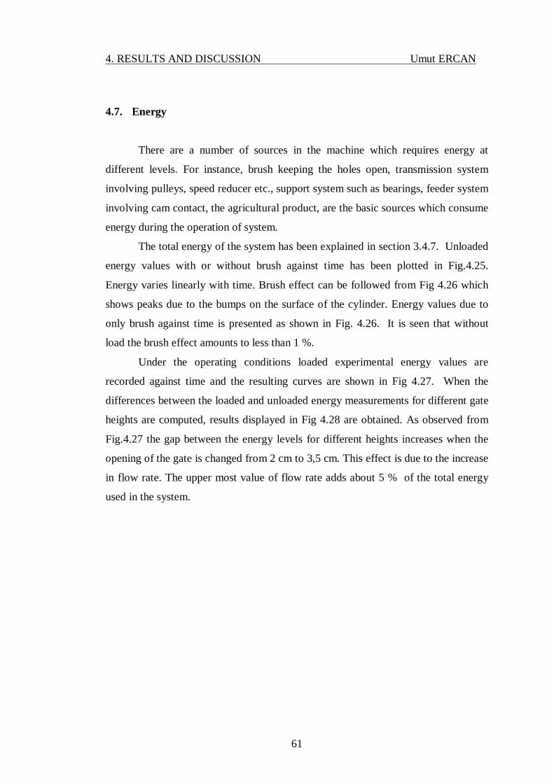
4. RESULTS AND DISCUSSION Umut ERCAN
61
4.7. Energy
There are a number of sources in the machine which requires energy at
different levels. For instance, brush keeping the holes open, transmission system
involving pulleys, speed reducer etc., support system such as bearings, feeder system
involving cam contact, the agricultural product, are the basic sources which consume
energy during the operation of system.
The total energy of the system has been explained in section 3.4.7. Unloaded
energy values with or without brush against time has been plotted in Fig.4.25.
Energy varies linearly with time. Brush effect can be followed from Fig 4.26 which
shows peaks due to the bumps on the surface of the cylinder. Energy values due to
only brush against time is presented as shown in Fig. 4.26. It is seen that without
load the brush effect amounts to less than 1 %.
Under the operating conditions loaded experimental energy values are
recorded against time and the resulting curves are shown in Fig 4.27. When the
differences between the loaded and unloaded energy measurements for different gate
heights are computed, results displayed in Fig 4.28 are obtained. As observed from
Fig.4.27 the gap between the energy levels for different heights increases when the
opening of the gate is changed from 2 cm to 3,5 cm. This effect is due to the increase
in flow rate. The upper most value of flow rate adds about 5 % of the total energy
used in the system.

4. RESULTS AND DISCUSSION Umut ERCAN
62
Figure 4.25 Energy values with or without brush vs time
Fig. 4.26 Loaded energy values vs time
010002000300040005000
6000700080009000
10000
0 20 40 60 80 100
Pow
er V
alue
s (W
h)
Time (s)
With Brush
without Brush
0
5
10
15
20
25
0 20 40 60 80 100
Ener
gy v
alue
s due
to b
rush
(Wh)
Time (s)
brush effect

4. RESULTS AND DISCUSSION Umut ERCAN
63
Fig. 4.27 Loaded experimental energy vs. time for different feeder gate heights
Fig. 4.28 Loaded energy values due to load vs time
0
2000
4000
6000
8000
10000
12000
0 20 40 60 80 100
Ener
gy v
alue
s (W
h)
Time (s)
2 cm
2,5 cm
3 cm
3,5 cm
0
100
200
300
400
500
600
700
800
900
0 20 40 60 80 100
Ener
gy v
alue
s due
to lo
ad (W
h)
Time (s)
2 cm
2,5 cm
3 cm
3,5 cm

4. RESULTS AND DISCUSSION Umut ERCAN
64

5. CONCLUSION Umut ERCAN
65
5. CONCLUSION
The ultimate goal of this work is to examine the sieving function of granular
material. Another goal of this study is to show the agreement between the theoretical
and experimental results. As a result of the experimental and theoretical calculations,
efficiency of the machine has been found to be very high and energy consumption
for this purpose has turned out to be low.
Kidney bean has been used as an agricultural product to investigate the
system behavior both theoretically and experimentally. In the following paragraphs
all the numerical values pertain to this product.
Efficiency of sieve maximum has been found to be between 99, 86 % and
98,64 % when feeder gate height is 2 cm. Similarly, minimum efficiency is 98,0 5%
to 95,25 % at the feeder gate height of 3,5 cm. Minimum feeder flow rate of the
feeder is 413,17 kg/h when feeder gate height is 2 cm. Maximum feeder flow rate is
2331, 60 kg/h at the feeder gate height of 3,5 cm. When the feeder gate height is
increased feeder flow rate increases. System control parameter is feeder gate.
Depending on the wish to operate the system at different efficiency level,
corresponding feeder gate height can be selected to satisfy certain flow rate and
efficiency conditions.
When there is no load on the system (i.e. no kidney bean) in the cylinder;
brushes require approximately 38 % of the driving torque applied on the machine.
The highest torque value due to load has materialized as 14,22 Nm at feeder gate
height of 3,5 cm . The lowest torque value has resulted as 5,22Nm, at feeder gate
height of 2 cm.
Under unloaded operating conditions the average brush consumption has
been found to be 9,03 W. Under loaded conditions power consumption over the
given time span has turned out to be 4,5 W and 19,41 W corresponding to the feeder
gate heights of 2 cm and 3,5 cm, respectively.
Energy consumption of cylindrical helical sieve within a period of 1.5 minute
due to load has been found to be 9,150 kWs when feeder gate height is 2 cm. Energy
consumption has increased to 9,633 kWs at a feeder gate height of 3,5 cm.
5. CONCLUSION Umut ERCAN
66
Experiments have shown that the helical sorting machine is operated under
very low power consumption with very high efficiency. It is observed that brushes
contribute to improve sorting function of the system. Despite some power
consumption they also lead to raise the efficiency level.
If the helical cylindrical sieve is manufactured carefully and properly, sorting
can be achieved with high efficiency and low energy consumption. Helical
cylindrical sieve can be utilized for sorting different granular material such as
peanuts, peas, soy beans etc.
In this work single and multi-layer models with linearly varying thicknesses
have been considered while developing the theory of the helical cylindrical sieve. It
is possible that multi layer models with non-linearly varying thickness can also be
taken into account.
This system has been used alone. However, it can be proposed to operate also
within an integrated system so as to include other food processes that depend on
sorting function.

67
REFERENCES
Akcali, I.D., Ince A., & Guzel, E. (2006). Selected physical properties of peanuts.
International journal of food properties, (9), 25–37.
Akcali, I.D., Guven, O. (1990). Physical properties of peanut in turkey, Agricultural
mechanization in Asia, Africa, and Latin America, (3) 55-60.
Alkhaldi, H., Eberhard, P. (2006). Computation of screening phenonema in a vertical
tumbling cylinder, Proceeding applied mathematics and mechanics, (6), 83–84.
Ata A. A., Rafeek A., Hanani Y., (2005). Sensory-based colour sorting automated
robotic cell, Journal of Intelligent and Robotic Systems, Springer, 43, 99–110.
Brosnan, T., Sun D.W.,(2002). Inspection and grading of agricultural and food
products by computer vision systems-a review. Computers and Electronics in
Agriculture 36 , 193-213.
Brosnan, T., Sun, D.W., (2004). Improving quality inspection of food products by
computer vision––a review, Journal of Food Engineering 61, 3–16.
Fellows, P. (2000). Food processing technology (2nd ed. pp.87). Cambridge,
England.
Feistritzer, W.P., Vock. H., & Reiter. H.(1981). Cereal and grain-legume seed
processing (Plant production and protection series no.21, pp. 77). Rome, Italy.
Grandison, A. S. (2006). Postharvest handling and preparation of foods for
processing. Brennan J. G. (Ed.), Food processing handbook (pp. 21).
Weinheim, Germany.
Guang-rong L., (2010) Rice color inspection based on image processing technique.
IEEE International Conference on Advances in Energy Engineering, 134 – 137.
Guzel, E., Akcali, I.D., & Ince A. (2007). Behavior of peanut bulk under static loads,
Journal of food engineering, (5), 385–390
Guzel, E., Akcali, I.D., Mutlu, H., & Ince, A. (2005). Research on fatigue behavior
for peanut shelling, Journal of food engineering, (3), 373–378.
Hongchang. L., Yaoming. L. (2011). Simulation and analysis of nonlinear motion for
material particles on vibrating screen, IEEE international conference
publication on new technology of agricultural engineering (ICAE), (5), 38-43.

68
He, X. M., Liu C. S. (2009). Dynamics and screening characteristics of a vibrating
screen with variable elliptical trace, Mining science and technology, (19),
0508–0513.
Narendra V. G., Hareesh K. S., (2010) Quality inspection and grading of
agricultural and food products by computer vision- a review. International
Journal of Computer Applications (0975 – 8887) Volume 2 – No.1, 43–65.
Lala, Z., Yuemin, Z., Liu Chusheng, Li Jun, & Hailin, D. (2011). Simulation of the
screening process on a circularly vibrating screen using 3d-dem, Mining
science and technology (China), (21), 677–680.
Shen, H. P., Li, J., Deng, J. M., Liu, Y. W., Ding, L., Zhang, J. T., Zhang, H. F., &
Yang, T. L. (2009). A novel vibration sieve based on the parallel mechanism,
IEEE 10th international conference publication on computer-aided industrial
design & conceptual design, (4), 2328-2332.
Shuang, C., Nian-qin G.,(2010). Optimization of super-heavy vibrating screen based
on MATLAB , IEEE 3rd International Conference on Information and
Computing,(3), 262 – 264.
Steyn J., (1995). Fatigue failure of deck support beams on a vibrating screen. J. Pres.
Vex & Piping, 61, 315-327.
Stoicovici, D. I., Ungureanu M., Ungureanu, N., & Banica M. (2009). Computer
model for sieves’ vibrations analysis, using an algorithm based on the false-
position method, American journal of applied sciences, (6) , 48-56.
Ronghua S.,, Liuqing Z.,, Chenyu P., (2010). CAE Applied to dynamic optimal
design for large-scale vibrating screen, IEEE 2010 First ACIS International
Symposium on Cryptography, and Network Security, Data Mining and
Knowledge Discovery, E-Commerce and Its Applications, and Embedded
Systems, 316 – 320.
Tan, J., Harrison H. P. (1987). Screening efficiency for planar and spatial drive
mechanisms, American society of agricultural engineers, 30(5), 1242-1253.
Unay, D., Gosselin, B., (2004). A qualıty sortıng method for ‘jonagold’ apples,
Engineering the Future (International Conference of Agricultural Engineering)
12-16 September 2004, Leuven, Belgium.

69
Yan, J., Liu, C., Zhao, L., Li, J., (2010). Parameters optimum design for linear
vibrating screen, IEEE International Conference on Computational and
Information Sciences, 413 – 415.
Yue-m, Z., Chu-sheng, L., Xiao-mei, H., Cheng-yong, Z., Yi-bin, W., Zi-ting, R.,
(2009). Dynamic design theory and application of large vibrating screen .The
6th International Conference on Mining Science & Technology, 2009
Published by Elsevier Procedia Earth and Planetary Science 1 , 776–784 .
Zhongjun, Y., Tian, H., Xin,S., Lianwan, Z., Research on dynamic characteristics of
elliptical vibrating screen, IEEE International Conference on Mechanic
Automation and Control Engineering (MACE), 2366 – 2369.
http://www.compacsort.com/wawcs0114832/idDetails=112/Internal/Taste%28N.I.R
%29.html (last access: 30.06.2012)

70

71
BIOGRAPHY
Umut ERCAN was born on July 08, 1983 in Adana, Turkey. He graduated
from High School In 2000, and enrolled at Fırat University to study mechanical
engineering. He graduated with a Bachelor of Science degree in mechanical
engineering from the Department of Mechanical Engineering in 2008. He began his
MSc studies at the Department of Mechanical Engineering of Çukurova University in
2008. He worked in İNSPEGO International Inspection & Certification Services Ltd.
2011 and 2012. He has been working as Research Assistant in the Automotive
Engineering Department of Batman University since February, 2012.