ultra-cold collisions and evaporative cooling of caesium ... · abstract ultra-cold collisions and...
TRANSCRIPT

Ultra-cold Collisions andEvaporative Cooling of Caesium
in a Magnetic Trap
Angharad Mair Thomas
A thesis submitted in partial fulfilment ofthe requirements for the degree of
Doctor of Philosophy at the University of Oxford
Jesus CollegeUniversity of Oxford
Hilary Term 2004

Abstract
Ultra-cold Collisions and Evaporative Cooling of
Caesium in a Magnetic Trap
Angharad Mair Thomas, Jesus College, Oxford University
DPhil Thesis, Hilary Term 2004
Caesium-133 atoms have been evaporatively cooled in a magnetic trap to tem-
peratures as low as 8 nK producing a final phase-space density within a factor
of 4 of that required for the onset of Bose-Einstein condensation. At the end of
the forced radio-frequency evaporation, 1500 atoms in the F = 3,mF = −3 state
remain in the magnetic trap. A decrease in the one-dimensional evaporative cool-
ing efficiency at very low temperatures is observed as the trapped sample enters
the collisionally thick (hydrodynamic) regime. Different evaporation trajectories
are experimentally studied leading to a greater understanding of one-dimensional
evaporation, inelastic collisions and the hydrodynamic regime. A theoretical sim-
ulation accurately reproduces the experimental data and indicates that the reduc-
tion in the evaporative cooling efficiency as the cloud enters the hydrodynamic
regime is the main obstacle to the realization of Bose-Einstein condensation in the
F = 3,mF = −3 state.
In addition, we report measurements of the two-body inelastic collision rate
coefficient for caesium atoms as a function of magnetic field and collision energy.
The positions of three previously identified resonances are confirmed, with reduced
uncertainties, at magnetic fields of 108.87(6), 118.46(3) and 133.52(3) Gauss. The
resonance centred at 118.46Gauss is also investigated as a function of temperature,
thus demonstrating the dependence of the inelastic Feshbach resonance on collision
energy. The importance of including partial waves of a higher basis in theoretical
i

closed channel calculations in order to accurately determine the line shape of a
Feshbach resonance is also demonstrated.
ii

Acknowledgements
This work could not have been carried out without the guidance and support
of a vast number of people.
My first thanks must go to my supervisor Prof. Christopher Foot who provided
me with the opportunity to work in his group and to study BEC which had first
intrigued me as an undergraduate. I greatly appreciate the work he has done
in reading through the various drafts of this thesis and for the suggestions and
comments which have crystallized my understanding.
Where would I be without Dr. Simon Cornish? Probably still taking slosh
data! His enthusiasm over the last three years has been boundless and his patience
limitless. My enjoyment of my time here in Oxford has been in no small part due
to his guidance and his friendship. He has also read my thesis carefully and offered
advice and corrections in making the thesis intelligible.
I must also thank Prof. Paul Julienne (NIST) for the theoretical data he
produced. If I absorb a hundredth of his understanding of ultra–cold collisions, it
would then become my chosen specialist subject in Mastermind.
Thank you to the present and past members of the group for not only being
willing to answer my questions, but actually answering them: Vincent, Gerald,
Onofrio, Donatella, Rachel and Eleanor. Thanks also to all the other members of
the group for providing some light in the dark basement.
The Clarendon staff must also be thanked for making my life easy: Sue, Gra-
ham, Terry, Dave and Alan in Stores, George and Rob in the Research Workshop,
Reg and all in the Main Workshop, D.T. Smith and all at Central Electronics,
Graham, Alan and Casper and everyone in maintenance.
iii

Over the past three years I have been very fortunate to have many good friends.
Special mention must go to Emma. Unsuccessful days in the lab were soon forgot-
ten over a glass of wine and an episode of ‘Friends’. I must also thank Edward for
his friendship and for proof–reading.
My last but by no means least thanks must go to my parents for their love and
continual support. Diolch yn fawr iawn am bopeth.
I must finish these acknowledgments with some words taken from the lab song:
“No one said it would be easy”
Sheryl Crow Tuesday Night Music Club (1993).
iv

Contents
1 Introduction 1
1.1 Bose-Einstein Condensation . . . . . . . . . . . . . . . . . . . . . . 1
1.1.1 Bosons and Fermions . . . . . . . . . . . . . . . . . . . . . . 2
1.1.2 Bose-Einstein Condensation . . . . . . . . . . . . . . . . . . 3
1.1.3 Experimental Observation . . . . . . . . . . . . . . . . . . . 4
1.1.4 Current Experiments . . . . . . . . . . . . . . . . . . . . . . 5
1.2 Caesium: State of Play – October 2000 . . . . . . . . . . . . . . . . 6
1.2.1 F = 4, mF = +4 . . . . . . . . . . . . . . . . . . . . . . . . 7
1.2.2 F = 3, mF = −3 . . . . . . . . . . . . . . . . . . . . . . . . 9
1.2.3 F = 3, mF = +3 . . . . . . . . . . . . . . . . . . . . . . . . 11
1.2.4 Recent Collisional Studies . . . . . . . . . . . . . . . . . . . 13
1.3 Overview of Thesis . . . . . . . . . . . . . . . . . . . . . . . . . . . 17
1.3.1 Notation . . . . . . . . . . . . . . . . . . . . . . . . . . . . . 17
1.3.2 Abbreviations Used in Thesis . . . . . . . . . . . . . . . . . 18
1.3.3 Constants and Conversion Factors . . . . . . . . . . . . . . . 18
1.3.4 Prior Publication of Work in this Thesis . . . . . . . . . . . 18
2 BEC: An Experimentalist’s Guide 21
2.1 The Recipe for Creating a BEC . . . . . . . . . . . . . . . . . . . . 21
2.2 Laser Cooling . . . . . . . . . . . . . . . . . . . . . . . . . . . . . . 23
2.2.1 Alkali Metals . . . . . . . . . . . . . . . . . . . . . . . . . . 23
2.2.2 Doppler Cooling . . . . . . . . . . . . . . . . . . . . . . . . . 26
v

CONTENTS vi
2.2.3 Sub-Doppler Cooling . . . . . . . . . . . . . . . . . . . . . . 27
2.3 Magneto-Optical Traps . . . . . . . . . . . . . . . . . . . . . . . . . 31
2.3.1 Six-Beam MOT . . . . . . . . . . . . . . . . . . . . . . . . . 31
2.3.2 Pyramidal MOT . . . . . . . . . . . . . . . . . . . . . . . . 33
2.4 Magnetic Trapping . . . . . . . . . . . . . . . . . . . . . . . . . . . 34
2.4.1 Zeeman Effect on the Hyperfine Ground States . . . . . . . 34
2.4.2 Simple Magnetic Trap . . . . . . . . . . . . . . . . . . . . . 35
2.4.3 Majorana Transitions . . . . . . . . . . . . . . . . . . . . . . 36
2.4.4 Ioffe-Pritchard Trap . . . . . . . . . . . . . . . . . . . . . . 37
2.4.5 Baseball Trap . . . . . . . . . . . . . . . . . . . . . . . . . . 39
2.4.6 Experimental Considerations . . . . . . . . . . . . . . . . . . 40
2.5 Evaporative Cooling . . . . . . . . . . . . . . . . . . . . . . . . . . 41
2.5.1 Radio-Frequency Evaporation . . . . . . . . . . . . . . . . . 41
2.5.2 Effects of Gravity on Evaporation . . . . . . . . . . . . . . . 42
2.5.3 Dimensionality of Evaporation . . . . . . . . . . . . . . . . . 44
3 Scattering Theory and Feshbach Resonances 46
3.1 Atomic Interactions . . . . . . . . . . . . . . . . . . . . . . . . . . . 46
3.1.1 Unperturbed Hamiltonian . . . . . . . . . . . . . . . . . . . 47
3.1.2 van der Waals Interaction and Exchange Terms . . . . . . . 47
3.1.3 Dipolar Interaction . . . . . . . . . . . . . . . . . . . . . . . 50
3.2 Scattering . . . . . . . . . . . . . . . . . . . . . . . . . . . . . . . . 52
3.2.1 Partial Wave Analysis . . . . . . . . . . . . . . . . . . . . . 52
3.2.2 Scattering Length . . . . . . . . . . . . . . . . . . . . . . . . 54
3.2.3 Scattering at Low Temperatures . . . . . . . . . . . . . . . . 55
3.3 Resonances . . . . . . . . . . . . . . . . . . . . . . . . . . . . . . . 56
3.3.1 Potential Resonances . . . . . . . . . . . . . . . . . . . . . . 57
3.3.2 Feshbach Resonances . . . . . . . . . . . . . . . . . . . . . . 59
4 Evaporative Cooling 62
4.1 Elastic and Inelastic Collisions . . . . . . . . . . . . . . . . . . . . . 63

CONTENTS vii
4.1.1 Elastic Collisions . . . . . . . . . . . . . . . . . . . . . . . . 63
4.1.2 Inelastic Collisions . . . . . . . . . . . . . . . . . . . . . . . 63
4.2 Efficiency of Evaporation . . . . . . . . . . . . . . . . . . . . . . . . 65
4.2.1 Hydrodynamic (Collisionally thick) regime . . . . . . . . . . 67
4.3 Evaporative Cooling Models . . . . . . . . . . . . . . . . . . . . . . 69
4.3.1 Simple Model of Evaporative Cooling . . . . . . . . . . . . . 70
4.3.2 Monte-Carlo Simulation . . . . . . . . . . . . . . . . . . . . 71
4.4 Evaporation Strategy . . . . . . . . . . . . . . . . . . . . . . . . . . 76
5 Experimental Apparatus 77
5.1 Apparatus . . . . . . . . . . . . . . . . . . . . . . . . . . . . . . . . 77
5.1.1 Lasers . . . . . . . . . . . . . . . . . . . . . . . . . . . . . . 77
5.1.2 Frequency Stabilization - DAVLL . . . . . . . . . . . . . . . 81
5.1.3 The Optical Table . . . . . . . . . . . . . . . . . . . . . . . 88
5.1.4 Vacuum System . . . . . . . . . . . . . . . . . . . . . . . . . 91
5.1.5 Pyramidal MOT . . . . . . . . . . . . . . . . . . . . . . . . 92
5.1.6 2nd MOT – Experimental MOT . . . . . . . . . . . . . . . . 95
5.1.7 Magnetic Trap . . . . . . . . . . . . . . . . . . . . . . . . . 97
5.1.8 Evaporation . . . . . . . . . . . . . . . . . . . . . . . . . . . 104
5.2 Control . . . . . . . . . . . . . . . . . . . . . . . . . . . . . . . . . 104
5.2.1 Experimental Synchronization . . . . . . . . . . . . . . . . . 104
5.2.2 Analogue Voltages . . . . . . . . . . . . . . . . . . . . . . . 105
5.3 Diagnostics . . . . . . . . . . . . . . . . . . . . . . . . . . . . . . . 107
5.3.1 Recapture . . . . . . . . . . . . . . . . . . . . . . . . . . . . 107
5.3.2 Absorption Imaging . . . . . . . . . . . . . . . . . . . . . . . 108
5.3.3 Comparison of Recapture and Imaging . . . . . . . . . . . . 112
5.4 Optimization and Characterization . . . . . . . . . . . . . . . . . . 113
5.4.1 Pyramidal MOT . . . . . . . . . . . . . . . . . . . . . . . . 113
5.4.2 Experimental MOT . . . . . . . . . . . . . . . . . . . . . . . 114
5.4.3 Loading the Experimental MOT . . . . . . . . . . . . . . . . 114

CONTENTS viii
5.4.4 Compressed MOT and Molasses . . . . . . . . . . . . . . . . 117
5.4.5 Optical Pumping . . . . . . . . . . . . . . . . . . . . . . . . 119
5.4.6 Calibration of Magnetic Trapping Parameters . . . . . . . . 120
6 Loss Measurements 124
6.1 Inelastic Feshbach Resonances . . . . . . . . . . . . . . . . . . . . . 125
6.1.1 Comparison of Theoretical and Experimental Data . . . . . 125
6.2 Feshbach Resonances in the F = 3,mF = −3 State . . . . . . . . . 126
6.2.1 Determination of the Two-Body Inelastic Collision Rate Co-
efficient . . . . . . . . . . . . . . . . . . . . . . . . . . . . . 126
6.2.2 Experimental Results . . . . . . . . . . . . . . . . . . . . . . 127
6.3 Temperature Dependence of the 118.5G Resonance . . . . . . . . . 130
6.3.1 Experimental Results . . . . . . . . . . . . . . . . . . . . . . 130
6.3.2 Theoretical Results . . . . . . . . . . . . . . . . . . . . . . . 133
6.3.3 Experimental and Theoretical Results . . . . . . . . . . . . . 135
6.3.4 Discussion . . . . . . . . . . . . . . . . . . . . . . . . . . . . 139
7 Evaporation Results 141
7.1 Initial Evaporative Cooling Attempt . . . . . . . . . . . . . . . . . 142
7.1.1 Experimental Procedure . . . . . . . . . . . . . . . . . . . . 142
7.1.2 Results . . . . . . . . . . . . . . . . . . . . . . . . . . . . . . 144
7.2 Two-Frequency Evaporation . . . . . . . . . . . . . . . . . . . . . . 148
7.2.1 Experimental Procedure and Results . . . . . . . . . . . . . 149
7.2.2 Discussion . . . . . . . . . . . . . . . . . . . . . . . . . . . . 150
7.2.3 Heating . . . . . . . . . . . . . . . . . . . . . . . . . . . . . 153
7.3 Very Weak Trap . . . . . . . . . . . . . . . . . . . . . . . . . . . . . 155
7.3.1 Experimental Procedure . . . . . . . . . . . . . . . . . . . . 155
7.3.2 Data Analysis . . . . . . . . . . . . . . . . . . . . . . . . . . 157
7.3.3 Results . . . . . . . . . . . . . . . . . . . . . . . . . . . . . . 159
7.3.4 Discussion . . . . . . . . . . . . . . . . . . . . . . . . . . . . 161

CONTENTS ix
8 Conclusion 163
8.1 Outlook . . . . . . . . . . . . . . . . . . . . . . . . . . . . . . . . . 164
A Bose-Einstein Condensation in Caesium 167
A.1 Experimental Setup . . . . . . . . . . . . . . . . . . . . . . . . . . . 167
A.2 Evaporation . . . . . . . . . . . . . . . . . . . . . . . . . . . . . . . 168
A.3 Comparison . . . . . . . . . . . . . . . . . . . . . . . . . . . . . . . 171
B Experimental Equipment Details 173
B.1 Computer Control Boards . . . . . . . . . . . . . . . . . . . . . . . 173
B.2 Electronic Equipment Details . . . . . . . . . . . . . . . . . . . . . 174
C Caesium Atomic Data and Experimental Equations 175
C.1 Atomic Parameters . . . . . . . . . . . . . . . . . . . . . . . . . . . 175
C.2 Magnetic Field Calculations . . . . . . . . . . . . . . . . . . . . . . 175
C.3 Number of Atoms . . . . . . . . . . . . . . . . . . . . . . . . . . . . 176

Chapter 1
Introduction
Since the earliest observations of Bose-Einstein condensation (BEC) in 1995 [1,
2, 3], numerous groups have observed quantum degeneracy in many different ele-
ments: rubidium (isotopes 87Rb [1] and 85Rb [4]), sodium [2], lithium (7Li [3] and
6Li [5, 6]), hydrogen [7], helium [8, 9] and potassium(41K [10] and 40K [11]). Until
very recently [12], a notable emission from this list was the alkali metal caesium.
What is Bose-Einstein condensation and why is it such an active area of re-
search?
1.1 Bose-Einstein Condensation
Bose-Einstein condensation was predicted in 1925 by Albert Einstein following
work by Satyendra Nath Bose. Bose derived the Planck’s black body radiation law
from Boltzmann statistics [13] by proposing that: photons could occupy different
states, photon number was not conserved and that by putting particles into cells
that there existed statistical independence of cells rather than particles. Initially,
the paper was rejected. However Bose then sent Einstein a copy of the paper, who
realised the importance of the work and arranged for it to be published. Einstein
then applied Bose’s results to material particles which are conserved, and published
many papers describing the statistics of these systems [14]. The consequence of the
work by Bose and Einstein was the prediction that a large occupation of particles in
1

1.1. Bose-Einstein Condensation 2
the ground state can occur. For low-density systems (approximately 1014 cm−3),1
the temperature at which quantum degeneracy is observed must be of the order
10−5 K or less.
1.1.1 Bosons and Fermions
Bosons are particles which have integer spin: the angular momentum of the par-
ticles is 0, h, 2h, 3h . . . A large proportion of atoms and all of the force carrying
particles (e.g. photons) are bosons. Fermions are particles which have half-integer
spin: the angular momentum of the particles is h/2, 3h/2, 5h/2 . . . Most of the el-
ementary building blocks of matter are fermions e.g. protons, neutrons, electrons.
Fermions obey the Pauli exclusion principle and therefore cannot occupy the same
quantum state, whereas there is no exclusion on the states a boson can occupy.2
Systems of bosons and fermions are described by different distributions. The
equations for these are given below (Equation 1.1). It is the presence of ± 1 in
the denominator that makes the physical results of these distributions so different
from one another.
ni =
1
exp ((εi − µ) /kBT )Maxwell− Boltzmann distribution
1
exp ((εi − µ) /kBT )− 1Bose− Einstein distribution
1
exp ((εi − µ) /kBT ) + 1Fermi−Dirac distribution
(1.1)
where ni is the average number of particles occupying a state i of energy εi and µ
is the chemical potential (the amount of energy required to add a particle to the
system).
1Dilute gases are an example of low-density systems.2In actual fact the presence of a boson in a quantum state increases the probability that
another boson will go into this state.

1.1. Bose-Einstein Condensation 3
1.1.2 Bose-Einstein Condensation
For a thermal collection of atoms, a large number of states are occupied. If the
temperature is lowered to below hω (where ω is the angular frequency of single
particle motion in a harmonic oscillator potential), most of the atoms in a system
are in the ground state. However, at a particular temperature called the critical
temperature (Tc), a large number of bosons occupy the ground state even when
the temperature is high enough for atoms to populate other states. Bose-Einstein
condensation is a quantum phenomena and it is the behaviour of bosons that makes
BEC possible.
According to wave-particle duality atoms have an associated wavelength, the
deBroglie wavelength:
λdB =
(h2
2πmkBT
)1/2
(1.2)
As atoms become colder their deBroglie wavelength increases. Bose-Einstein con-
densation occurs when the deBroglie wavelength is comparable to the inter-particle
separation (n−1/3) and the wavefunctions of the atoms overlap. The condition for
BEC for a gas in free space is when the phase-space density (PSD) exceeds 2.612:
nλ3dB ≥ 2.612 (1.3)
where n and T (Equation 1.2) are the density and temperature of the gas re-
spectively. In BEC experiments a dilute vapour is non-uniform as the atoms are
contained in a trap. The critical temperature Tc is given by:
kBTc = 0.94hωN1/3 (1.4)
To illustrate that BEC occurs when the temperature is high enough for oc-
cupation of many harmonic oscillator states, N = 1 × 10⁶ is substituted into
Equation 1.4:
kBTc ≈ 100(hω)
Condensation can occur even when 100 harmonic oscillator states are occupied. If
ω is 1× 10³ s−1 then the critical temperature is 4.5 µK.

1.1. Bose-Einstein Condensation 4
For an ideal system, the wavefunction of a BEC of N atoms is the product
of N single particle wavefunctions. For a cloud of atoms with interactions, the
non-linear Schrodinger equation includes a term due to the mean-field energy (U0)
of the condensate:
U0 =4πh2na
m(1.5)
where a is the scattering length (see Chapter 3). The sign of a and therefore the
mean-field energy determines the stability of a condensate. For a positive a the
interactions are repulsive and therefore the condensate can be arbitrarily large.
In contrast, for a negative a the interactions are attractive and the condensate is
unstable for a large number of atoms.
1.1.3 Experimental Observation
In 1938 Fritz London suggested that the observation of superfluidity when helium-
4 was cooled to its lambda point3 could be attributed to Bose-Einstein conden-
sation. London’s suggestion met with skepticism as Einstein’s theory predicted
condensation for non-interacting particles whereas the atoms interact strongly in
liquid helium. The helium system is difficult to understand on an elementary level
because of the strong interactions therefore it was a long-sought goal to observe
Bose-Einstein condensation in a vapour.
The signature of BEC is the appearance of a narrow peak in both coordinate
and momentum space. When a condensate is confined in an elliptically shaped
potential, on release from the magnetic trap the short direction expands faster
than the long direction and therefore after a time the cloud is elongated in the
previously short direction. There are two factors that cause the aspect ratio to be
inverted: the dominant effect in normal BEC experiments is the repulsive inter-
atomic interactions while the Heisenberg uncertainty principle4 is dominant in
non-interacting condensates. A thermal cloud does not behave in this manner and
therefore upon release from the magnetic trap it becomes isotropic in space.
3The lambda point is equivalent to the critical temperature in dilute gases.4The more precisely the position is determined, the less precisely the momentum is known.

1.1. Bose-Einstein Condensation 5
It took until 1995 for Bose-Einstein condensation in a gas to be observed [1, 2,
3]. A dilute atom vapour condensate can be described as a near ideal gas (weakly
interacting system) as the inter-particle separation is much larger than the particle
size. The observation of a gaseous condensate created a test bed for theories that
described non-interacting systems.
1.1.4 Current Experiments
Since the observation of BEC in 1995, the research field has grown and blossomed.
The paths which the experiments have taken are many and diverse. For example, a
demonstration of an atom laser5 has already been observed at MIT [15]. The areas
of physics involved in some aspect of BEC research already include: atomic physics,
quantum optics, statistical mechanics, condensed matter physics and quantum
computing.
The first observation of a Feshbach resonance in a BEC [16] led to some very
exciting physics. Atom-atom interactions could be tuned leading to the possibility
of examining repulsive, attractive and non-interacting systems. The existence of a
Feshbach resonance in the scattering structure of 85Rb allowed for the creation of a
BEC [4]. Using the magnetic tunability of the Feshbach resonance the 85Rb group
at JILA have studied the collapse of the condensate [17, 18] and have created a
quantum superposition of atoms and diatomic molecules [19].
The most recent developments have been the creation of molecular condensates
by groups at Innsbruck [5], JILA [20], and MIT [6]. Each group starts with a cloud
of Fermi atoms (6Li at Innsbruck and MIT, 40K at JILA) and evaporatively cool
their sample before creating molecules and detecting them by use of a Feshbach
resonance. Molecules cannot be imaged directly and therefore the existence of
molecules is inferred by imaging the atoms created by disassociating the molecules
by sweeping the magnetic field across a Feshbach resonance.
Condensation of fermionic atom pairs in the BCS-BEC crossover regime has
been observed [11]. The previous experiments had demonstrated BEC of molecules
5Atoms in a BEC are coherent due to the overlap of the atoms’ individual wavefunctions.

1.2. Caesium: State of Play – October 2000 6
which is the extreme end of the BCS-BEC crossover and is created by approaching
the Feshbach resonance from the positive scattering length side of the resonance.
Jin et al. observe condensation on the other side of the resonance (a < 0). On this
side the formation of dimers is not supported and therefore condensation occurs
due to many-body effects. The observation of a condensate of fermionic atom pairs
occurred at the beginning of 2004, paving the way for studies of superfluidity (the
crossover between conventional superfluidity and the superfluidity of molecules),
and created another novel system for the testing of theories. 2004 promises to be
another year of exciting and valuable physics.
This is the current situation, however what was the situation when this work
began? The next section is a review of the work to condense caesium since the
early days of BEC experiments.
1.2 Caesium: State of Play – October 2000
Caesium, a heavy alkali metal atom, is well suited to laser cooling experiments
because of its small photon recoil (see Table 1.1 for the atomic parameters of
133Cs). The low temperatures that had been attained in laser cooling experiments
made caesium an obvious choice, not only for BEC experiments but for cold atom
studies.
Electronic Configuration [Xe]6s1
Atomic Number 55Atomic Weight 132.905Nuclear Spin, I 7/2
Table 1.1: Atomic parameters of caesium-133
The benefits of using slow atoms for precision spectroscopy have been recog-
nized for many years. By using laser cooled Cs atoms at µK temperatures, the
accuracy and stability of the caesium frequency standards were improved by two to
three orders of magnitude [21]. However, the nature of Cs collisions at low temper-
atures is unusual. In the ultra-cold regime, the deBroglie wavelength is larger than

1.2. Caesium: State of Play – October 2000 7
the scale of the interatomic potential. The scattering is therefore quantum me-
chanical in nature and is usually dominated by the lowest allowed partial angular
momentum wave (s-waves) [22]. It is important to understand these ultra-cold col-
lisions as sizeable frequency shifts between the two hyperfine states of the ground
state of Cs (the so-called “clock transition”) can occur and affect frequency stan-
dards. The telecommunications industry relies heavily on timing and therefore
frequency shifts in the “clock transition” cause inaccuracy. Also, most other units,
including the metre, are defined in terms of the second.6
The study of ultra-cold collisions is not only useful for metrologists, but also
for BEC experimentalists. Understanding inter-atomic collisions is important for
the optimization of the evaporation of an atom cloud.
Caesium was the early leader in the race to BEC due to the low temperatures
that had been achieved by laser cooling alone, and was also predicted to have
favourable scattering properties for Bose condensation in the (3,−3) state [23].
However, it was soon overtaken by most of the other alkali metals. Why was
caesium so difficult to condense?
1.2.1 F = 4, mF = +4
The early experimental attempts to Bose-condense caesium focussed on the mag-
netically trappable F = 4, mF = +4 state where the destructive spin relaxation
process is forbidden (see Section 3.1, Chapter 3). Instead, the dominant loss mech-
anism was expected to be the much weaker dipole relaxation occurring through
the magnetic dipole-dipole interaction.
However, attempts at evaporative cooling of atoms in this state failed com-
pletely. The highest PSD attained was 10−5 for a cloud at a temperature of
4µK [24]. The failure could not be attributed to background gas collisions or
heating due to experimental noise e.g. stray light, noise on magnetic fields etc.
It therefore became clear that the collisional behaviour was far from what had
been anticipated. Attention then turned to measuring the elastic and inelastic
6The second is defined as the duration of 9,192,631,770 periods of the radiation correspondingto the transition between two hyperfine levels of the ground state of the caesium-133 atom.

1.2. Caesium: State of Play – October 2000 8
collision rate coefficents for 133Cs in the F = 4, mF = +4 state [25, 26]. Two-
body inelastic collision rate coefficients for other cold alkali metals such as lithium,
sodium and rubidium in their doubly-polarized state ranged from 6 to 20 × 10−15
cm3 s−1 [27, 28, 29]. It was predicted that the value for doubly-polarized Cs would
be in the same range [30, 23].
Foot et al. (Oxford) studied the two-body inelastic collisions at a magnetic
field of 7G [31]. At a temperature of 30 µK they obtained a value for K2 of
1.2 × 10⁻¹¹ cm3 s−1 [26]. In a supplementary experiment they allowed the cloud
to evolve in the magnetic trap and periodically probed the cloud with σ+ light on
the F = 4 → F ′ = 5 transition. They observed an increase in the atom number
compared to when the cloud was allowed to evolve in the dark in the magnetic
trap. Graphs of number plotted against time for both cases gave a non-exponential
decay for the non-probing case and a purely exponential decay for the probed case.
Non-exponential behaviour is a signature of a multi-body decay process. This
implied that the two-body inelastic loss rate had been completely suppressed. The
conclusion was that at fields of ≈ 7G, decay to other mF states was occurring.
This seemed to agree with the observation of a zero-energy resonance [25].
Dalibard and co-workers (ENS, Paris) measured a value for the two-body in-
elastic collision rate coefficient, K2 [24]. After allowing a cloud of atoms in the
(4, +4) state to relax in the magnetic trap they imaged the cloud and plotted
atom number against evolution time. The evolution of the atom number exhibited
non-exponential behaviour. The value obtained for the two-body inelastic collision
rate coefficient at a magnetic field of 1.5G and at temperatures ranging from 8 to
70µK was:
(1.5± 0.3± 0.3)× 10−11T−0.63 cm3 s−1
Therefore at a temperature of 8 µK, the two-body inelastic collision rate coefficient
is 4× 10⁻¹² cm3 s−1. This value is three orders of magnitude higher than the pre-
dicted value [23, 30]. The experimental value obtained was also the same order
of magnitude as the two-body inelastic collision rate coefficient for unpolarized

1.2. Caesium: State of Play – October 2000 9
F = 4 atoms. However, that rate could be accounted for by spin relaxation. Dal-
ibard and co-workers then postulated that the atoms were decaying via hyperfine
changing collisions. To validate the postulate they performed another experiment.
Before imaging the atoms they reduced the field gradient of the magnetic trap to
a value that still trapped the mF = 4 state but not the other mF states. If other
substates were present in the trap they would be seen at a different position on the
CCD array as they fell under the influence of gravity. However, no extra clouds
were observed. To check their results they performed the same experiment again
but this time with a cloud of F = 4 depolarized atoms. Images taken this time
showed small clouds of atoms falling under the influence of gravity. These clouds
corresponded to the mF = 3, 2, 1 states. This confirmed that nearly all the atoms
were lost via hyperfine-changing collisions. They explained this observation in
two complementary fashions. Firstly, the presence of a zero-energy resonance [25]
increases the two-body inelastic collision rate. Secondly, for heavy alkali metals,
dipole relaxation can occur due to the second-order spin-orbit interaction (Sec-
tion 3.1, Chapter 3). The second-order spin-orbit interaction was neglected from
early predictions [23, 30] but recent calculations that take this effect into account
reproduced the results of References [24, 25]. This behaviour completely explained
why evaporative cooling does not work in the F = 4, mF = 4 state.
1.2.2 F = 3, mF = −3
Following the realization that the two-body inelastic loss rates were too high to
achieve BEC in the F = 4, mF = +4 state, attention turned to the lower hyperfine
state and the magnetically trappable F = 3, mF = −3 state. It had been shown
that this state had favourable scattering properties for BEC and it was also pre-
dicted that it would show pronounced resonance structure [23]. This meant that
by varying the magnetic field it would be possible to vary the magnitude and sign
of the atom-atom interactions.
Monroe et al. had measured the elastic collision cross-section and the two-body
inelastic collision rate coefficient for spin polarized atomic caesium in 1993 [32].

1.2. Caesium: State of Play – October 2000 10
A value of 1.5(4) × 10−12 cm2 for the zero-energy s-wave elastic cross-section was
obtained and it was stated that the cross-section was independent of temperature
between 30 and 250 µK. An upper limit of 5× 10⁻¹⁴ cm3 s−1 was put on the two-
body inelastic collision rate coefficient. Tiesinga et al. calculated the two-body
inelastic collision rate coefficient, and obtained a value of 1 × 10⁻¹⁵ cm3 s−1 [23],
which was consistent with, although much smaller than the upper limit obtained
previously. It was suggested that the limiting loss process was not dipole relaxation
or molecular formation but collisions with background gas [32].
Initial attempts to condense Cs in the F = 3, mF = −3 state failed because
the inelastic loss rates were still unusually high. However, the suppression of the
dipole relaxation collisions as the magnetic field tends to zero (Section 3.1.3, Chap-
ter 3) meant there was some experimental success, most notably in Paris [33] and
Oxford [26]. Although the experiments used different trapping geometries,7 both
worked at low magnetic fields around 1G to take advantage of the suppression
of the two-body inelastic collisions. The group in Paris simulated their evapo-
ration [34] and predicted that they would obtain BEC with over 5 000 atoms.
Unfortunately, they only achieved a PSD of 3 × 10⁻², two orders of magnitude
below the condensation threshold. Both groups concluded that the efficiency of
evaporation was insufficient for obtaining BEC because the rate of two-body in-
elastic collisions was still too high. Subsequent analysis by ourselves illustrated
that the atom cloud was entering the hydrodynamic regime in the last evaporation
stages of their experiments (Section 4.2.1, Chapter 4).
Study of the two-body inelastic losses showed that the dipole relaxation rate
increased rapidly with increasing magnetic field between 1 and 7G [35]. It was
suggested that this increase could be due to the existence of a Feshbach resonance
close to B = 0G [36].
The magnitude and sign of the scattering length for the (3,−3) state was
determined in 2000 [37, 38] and confirmed the earlier prediction of the existence of
7The Oxford experiment used a time-averaged orbiting potential (TOP) trap with ωtrap =23 Hz and B < 1 G. The Paris experiment operated a Ioffe-Pritchard (I-P) type trap with ωtrap =38 Hz and B = 1.2G.

1.2. Caesium: State of Play – October 2000 11
a Feshbach resonance close to B = 0 G.8 The scattering length of Cs in the (3,−3)
around 1G is large and negative which explained the failure to condense Cs in the
experiments operating at approximately 1G.
1.2.3 F = 3, mF = +3
Following the failure to condense caesium in any of the weak-field seeking states,
recent attempts, including Salomon – ENS Paris [39], Vuletic and Chu – Stan-
ford [40], Weiss – formerly at Berkeley [41] and Grimm – formerly at Heidel-
berg [42], turned towards dipole force trapping of the F = 3, mF = +3 state.
As this is the lowest energy magnetic sublevel, inelastic two-body collisions are
energetically forbidden.
Salomon et al. used a Raman cooling scheme in a red-detuned crossed dipole
trap to simultaneously cool and polarize 133Cs atoms. They achieved a temperature
of 2.4µK with 2.5 × 10⁴ atoms in the (3,+3) state. This corresponds to a PSD
of 10−3 [39]. They believed that the highest PSD they achieved was limited by
multiple photon scattering in the atomic cloud.
Vuletic/Chu et al. achieved temperatures close to the photon recoil limit in a
3D far-detuned optical lattice. They succeeded in transferring 95 % of the atoms
from the MOT into the lattice while simultaneously spin-polarizing and cooling
the atoms. The cooling is achieved with 3D degenerate Raman sideband cooling.
They attained temperatures of 290 nK with 3×10⁸ atoms (80% of these atoms are
in the lowest vibrational bands of the lattice) at a density of 1.1× 1011 cm−3. This
corresponds to a PSD of 1/500 [40]. This experiment succeeded in laser-cooling a
large number of caesium atoms to a high phase-space density.
Weiss et al. laser-cooled 5×10⁷ Cs atoms to a PSD of 1/30. This was achieved
in a 3D far-off-resonant lattice (FORL). They compressed the cloud and performed
polarization gradient cooling followed by 3D Raman sideband cooling. In a FORL
the heating due to rescattered photons is suppressed when the vibrational fre-
quency exceeds the light scattering rate [43]. The highest PSD that could be
8The actual position of the resonance is -17 G.

1.2. Caesium: State of Play – October 2000 12
obtained was limited by photon rescattering. However, they predicted that with
consideration of the depth of the FORL and careful application of laser cooling
they could achieve BEC with laser cooling alone.
Grimm et al. implemented two different experiments in order to pursue the
quest of condensing caesium.9 The first experiment is a gravito-optical surface
trap (GOST) [44], where atoms are cooled above an evanescent-wave atom mirror.
They start with approximately 107 atoms at a temperature of 10 µK. Following
an evaporation stage they reach a temperature of 300 nK with 3 × 10⁴ atoms
remaining. This corresponds to a PSD of 3 × 10⁻⁴. This PSD could be increased
by a factor of 7 if the atoms were polarized into the F = 3, mF = +3 state. The
main advantages of a GOST is that it has a large trapping volume and therefore
many atoms can be captured. Following this experiment they implemented a
double evanescent-wave (DEW) trap [45] and achieved a temperature of 100 nK
with 20 000 atoms at a PSD close to 0.1. The experiment was limited mainly by
two factors. Firstly, the atoms were not polarized and therefore two-body inelastic
collisions were causing heating and trap loss. Secondly, when the dimensionality
of the atom cloud was approaching two, atoms were not being evaporated out
of the trap vertically. To overcome these difficulties involved two modifications.
Polarizing the atoms into the F = 3, mF = +3 state would not only eliminate
two-body inelastic collision loss but would allow for the tuning of the scattering
length using magnetic fields. Also, magnetic field gradients could compensate for
gravity allowing for evaporation vertically from the trap.
Their second experiment is evaporation of caesium in a quasi electrostatic dipole
trap (QUEST). Cs atoms are trapped in the focus of a CO2 laser beam. A CO2
laser has a wavelength of 10.6µm which is far from any optical transitions from
the ground state of Cs. This has two main advantages: the optical potential
becomes quasi electrostatic which means that different atomic species and even
molecules can be confined in the trap and, because of the large detuning from
resonance, the photon scattering rate is negligibly small and therefore heating
9Both schemes have now succeeded in condensing Cs (Appendix A).

1.2. Caesium: State of Play – October 2000 13
associated with photon momentum recoil which normally occurs in dipole traps is
suppressed. In the year 2000, Grimm et al. observed a reduction in temperature
of approximately a factor of two over approximately 150 s. This was due to plain
evaporation i.e. evaporation from a trap at constant trap depth. There were
three fundamental problems prohibiting further progress towards condensing Cs.
The first was that the cross-section is temperature dependent which increases the
thermalization time [25]. The second problem was gravity. The presence of gravity
can make evaporation one-dimensional leading to a reduction in the efficiency of the
evaporation [46](see Chapter 4). The third problem was the high rate of inelastic
loss due to three-body collisions.
In 2002, Grimm and co-workers at Innsbruck overcame the difficulties and
successfully condensed caesium into the absolute ground state [12]. Crucial to
their success is the implementation of an efficient final stage of evaporative cooling
to combat the three-body problems.10
1.2.4 Recent Collisional Studies
The early experiments took place during a period when the collisional properties of
caesium were poorly understood, because of a combination of a lack of experimental
data and difficulty in calculating the properties for such a large atom. The van der
Waals coefficient C6 [47] and the magnitude of the indirect spin-spin coupling [48]
were not known and therefore it was impossible to even determine whether the
atom-atom interactions were repulsive or attractive. However, in the year 2000,
two papers were published which stated accurately for the first time the cold-
collision properties of 133Cs.
Vuletic/Chu et al. observed over 25 resonances in the magnetic field range
0 to 230G and accurately measured the positions of these resonances to within
30mG [38]. Feshbach spectroscopy has a high resolution because it only involves
electronic ground states and is therefore limited solely by the temperature of the
sample. They have the ability to prepare atoms in various hyperfine and magnetic
10Appendix A contains a description of the experiment at Innsbruck, and a comparison of theproblems and results in Innsbruck and Oxford.

1.2. Caesium: State of Play – October 2000 14
sublevels and they can probe different parts of the molecular potential. They
observed that the (4, +4) state has no resonance and that at a temperature of
5µK the two-body inelastic collision rate coefficient is 2 × 10⁻¹² cm3 s−1 which is
in agreement with the value given in Reference [24].
The subsequent theoretical analysis at NIST, Gaithersburg provided for the
first time an accurate characterization of the collisional properties of caesium [37].
They extracted values for the singlet and triplet scattering lengths and a value for
the van der Waals coefficient. These values are given in Table 1.2.
Name Symbol ValueSinglet scattering length X1Σ+
g 280± 10 a0
Triplet scattering length a3Σu 2400± 100 a0
van der Waals coefficient C6 6890 ± 35 a.u.
Table 1.2: Values for the collisional properties of caesium [37].
The value obtained for the F = 4, mF = 4 scattering length was 2400± 100 a0
which was not only different in magnitude but also in sign to what had been
predicted previously [23, 30, 36].
To model the resonances Leo et al. [37] used a coupled channel theoretical model
similar to the model described in References [48, 49]. Their analysis reproduced all
of the (3,−3) × (3,−3) inelastic resonances between 0 and 250G. Figure 1.1 is a
plot of the scattering length, two-body inelastic losses, and the elastic collision rate
coefficient against magnetic field for the (3,−3) state. The magnitude of the two-
body inelastic collision rate coefficient for 85Rb at 162.5 G is also included on the
plot.11 This clearly illustrates the difficulties facing experimentalists attempting
to condense Cs as the two-body inelastic collision rate coefficient in the (3,−3)
state is an order of magnitude greater than for 85Rb which is considered to be a
challenging isotope to condense.
The theoretical analysis predicted two-body collisional properties with a high
degree of confidence and suggested that 133Cs F = 3, mF = |3| possessed suitable
11The 85Rb experiment at JILA evaporate at a magnetic field of 162.5 G.

1.2. Caesium: State of Play – October 2000 15
025
5075
100
125
150
175
200
225
250
1E-14
1E-13
1E-12
1E-11
1E-10
1E-9
1E-8
01000
2000
3000
4000
5000
K2 85
Rb
(162
.5G
, 0.5
K)
0.05
K0.
5K
1.0
K2.
5K
5.3
K
Scattering Length (a0)
Collision Rate Coefficient (cm3s
-1)
Mag
netic
Fie
ld (G
)
Figure 1.1: The solid and dotted coloured lines denote the two-body inelastic collisionrate coefficient (K2) and the elastic collision rate coefficient respectively at the giventemperatures. The thick black line denotes the scattering length. The shaded sectionsillustrate where the scattering length is negative. For comparison, the dotted line at avalue of K2 = 7 × 10⁻¹⁴ cm3 s−1 is the two-body inelastic collision rate coefficient for85Rb at 162.5 G and at a temperature of 0.5µK. Data for the figure obtained from [50].

1.2. Caesium: State of Play – October 2000 16
scattering properties for BEC [37].

1.3. Overview of Thesis 17
1.3 Overview of Thesis
The aim of the work carried out in this thesis was to condense caesium in a magnetic
trap. A new experiment was built in order to pursue this quest – the general
discussion of the techniques is given in Chapter 2 while the experimental details
are given in Chapter 5.
To decide on the evaporation strategy it is crucial to understand the nature of
the inter-atomic collisions. Chapter 3 describes the origin of some of the scattering
properties of caesium. It includes a description of the inter-atomic potential, the
origin of elastic and inelastic collisions and the occurrence of resonances, both
potential and Feshbach resonances. Three Feshbach resonances were observed
and characterized during this work. The temperature dependence of one of these
resonances was also studied. These results are given in Chapter 6.
In many alkali metal BEC experiments, there is a great tolerance in the choice of
magnetic trap and magnetic trapping parameters.12 For caesium however, because
of the high inelastic losses, the choice of magnetic trap and especially the magnetic
trapping parameters has a large effect on the evaporation performance. Chapter 4
is a discussion of the theoretical principles of evaporative cooling. It includes a
summary of the elastic and inelastic losses in a trapped atom cloud, the effect that
trap frequencies and the scattering length has on these losses, and the methods
used to simulate the evaporation. The experimental results of our attempt to
condense caesium are included in Chapter 7.
1.3.1 Notation
Some of the less obvious notations used in the thesis are given below:
• When the phase-space density (PSD) is stated, the value is normalized so
that the BEC transition in a confining potential occurs at a PSD of unity.
• When the rf power is quoted, it is value of the output power of the rf synthe-
12To achieve BEC there must be no B=0 G in the magnetic potential. It is also beneficial tohave a tight trap to increase the efficiency of the evaporation.
1.3. Overview of Thesis 18
sizer before the amplifier unless stated otherwise. The amplifier has a gain
of 40 dB.
• When discussing electrons, unless otherwise stated, the comment refers to
the valence electron.
• The magnetic field is always expressed as B with units of Gauss (≡ 10−4 T).
• The current is always quoted in Amperes (A).
• Vector quantities are represented by bold characters.
• An atom cloud, cloud of atoms etc. refers to a collection of atoms trapped
in or released from a magnetic trapping potential.
1.3.2 Abbreviations Used in Thesis
Many abbreviations are used throughout the thesis. The first mention of an ab-
breviation is always accompanied with the full name, however for completeness
Table 1.3 contains all of the abbreviations used in this work.
1.3.3 Constants and Conversion Factors
Table 1.4 contains all the common constants and conversion factors used in the
thesis. Table C.1, Appendix C contains all the values for the relevant atomic
properties of caesium.
1.3.4 Prior Publication of Work in this Thesis
Several of the results described in this thesis have been published in journals.
Section 6.2.2, Chapter 6 and Section 7.1, Chapter 7 appears in Reference [51].
The work in Section 7.3, Chapter 7 appear in Reference [52].

1.3. Overview of Thesis 19
AOM - Acousto-optic modulatorPZT - Piezoelectric transducerFET - Field effect transistorswg - Standard wire gaugeTTL - Transistor-transistor logicPSD - Phase-space densityrf - Radio-frequency
JILA - Joint Institute of Laboratory AstrophysicsNIST - National Institute of Standards and TechnologyMIT - Massachusetts Institute of TechnologyBEC - Bose-Einstein condensationGPIB - General purpose interface busPCI - Peripheral component interconnectCCD - Charge-coupled device
FWHM - Full width at half maximumTOP - Time-averaged orbiting potentialNEG - Non-evaporable getterMOT - Magneto-optical trap
CMOT - Compressed magneto-optical trapOP - Optical pumping
DSPOT - Dark spontaneous-force optical trap3D - Three-dimensional
DEW - Double evanescent-waveFORL - Far-off-resonant latticeGOST - Gravito-optical surface trap
I-P - Ioffe-PritchardQUEST - Quasi electrostatic dipole trapMOPA - Master oscillator power amplifierECDL - External cavity diode lasersrms - Root mean square
DAVLL - Dichroic atomic vapour laser lockTOF - Time-of-flightOD - Optical depth
Table 1.3: Abbreviations used in thesis

1.3. Overview of Thesis 20
1 Tesla ≡ 104 GaussBohr radius, a0 = 0.5291772108× 10⁻¹⁰ m
Planck constant, h = 6.6260693× 10⁻³⁴ J sBohr magneton, µB = 927.400949× 10⁻²⁶ J T−1
= 1.4 MHz G−1
Speed of light, c = 299 792 458 m s−1
Boltzmann constant, kB = 1.3806505× 10⁻²³ J K−1
Permeability of free space, µ0 = 4π × 10−7 m kg s−2 A−2
Gravitational acceleration, g = 9.81 m s−2
Table 1.4: Conversion factors and common constants used in thesis.

Chapter 2
BEC: An Experimentalist’s Guide
Bose-Einstein condensation was predicted in 1925 [14], but it took until 1995 for it
to be experimentally realised in dilute gases [1, 2, 3]. It was necessary to develop
many experimental techniques over the 70 years between the prediction and the
experimental realisation of BEC. This section gives a brief review of these tech-
niques. The discussion of theoretical principles is limited as they have been covered
extensively in the literature and numerous theses.
2.1 The Recipe for Creating a BEC
There is no single definitive way of producing a Bose-Einstein condensate – each
group have their own favourite ingredients. The different ingredients, however
must be added in the correct order. Figure 2.1 illustrates the most common routes
to BEC.
All experiments involve a collection stage where large numbers of cold atoms
are loaded into the experimental magneto-optical trap (MOT) in the ultra-high
vacuum region. The atom collection generally occurs in a magneto-optical trap
(extracted from a vapour) or is generated by use of a Zeeman slower.
The workhorse of most BEC experiments is the experimental MOT (see Sec-
tion 2.3) where most of the cooling in absolute terms is carried out. Following
laser cooling in the MOT it is necessary to cool the atoms further by including
21

2.1. The Recipe for Creating a BEC 22
MOT
Zeemanslower
Collection MOT Magnetic
trap
Optical Trap
EvaporationOptical Pumping
Low magnetic field-seeking states
High magnetic field-seeking
states
Imaging
BEC
UHV Region
Figure 2.1: The path to Bose-Einstein condensation. (MOT – denotes magneto-opticaltrap.)
an optical molasses stage when the magnetic field is turned off and the cloud is
allowed to expand and cool.
It is important to load a large number of atoms at a high density into the
magnetic or optical trap as the evaporative cooling rate depends on the collision
rate1 on loading the trap. Many groups therefore implement variations in the MOT
scheme or add additional stages to reduce the temperature or increase the density
in the MOT.2
Atoms in a MOT are distributed across all magnetic sublevels, therefore prior to
loading the magnetic trap, atoms must be polarized into weak field-seeking states
(Section 2.4). This is accomplished with an optical pumping (OP) pulse. This not
only polarizes the atoms it also pumps the atoms into fully polarized states3 which
reduces the likelihood of inelastic collisions (see Chapter 3).
In 1986, Chu et al. [54] experimentally realised another form of an atom trap
– an optical trap. The neutral atoms are trapped by the interaction of the electric
dipole with far-detuned laser radiation. An excellent review article of optical dipole
traps is Reference [55].
1The elastic collision rate depends linearly on the density, therefore evaporation proceedsfaster the higher the density (see Chapter 4).
2A dark spontaneous-force optical trap (DSPOT) [53] is an example of a method to increasethe density in the MOT. A DSPOT confines atoms in a ‘dark’ state which reduces the force dueto reradiation of atoms at the centre of the cloud (radiation pressure).
3For low field-seeking states (mF gF < 0), and high field-seeking states (mF gF > 0), fullypolarized denotes states where F = |mF |.

2.2. Laser Cooling 23
Following the confinement of the atoms, they must be cooled further in order
to achieve the temperatures required for condensation (Section 2.5). If atoms with
energy greater than the average energy are removed from the trap, the remaining
atoms rethermalize to a lower temperature through elastic collisions. By selectively
removing the hot atoms from the trap the gas is evaporatively cooled [56].
With careful optimization of all experimental parameters, a sharp peak in the
density profile of the atom cloud is seen upon imaging which is the signature of
the formation of a Bose-Einstein condensate.
Following the difficulty in condensing caesium, the BEC recipe had to be tai-
lored especially for the purpose of condensing caesium in the F = 3, mF = −3
state. Each ingredient had to be understood individually to combine these tech-
niques effectively in order to optimize the experiment. Some of the ingredients
are discussed below (Sections 2.2, 2.3, 2.4, and 2.5) whereas a discussion of the
evaporative cooling considerations is given in Chapter 4.
2.2 Laser Cooling
Laser cooling of atoms was first proposed in 1975 [57], but not experimentally
realised until 1985 [58]. The first neutral atom element to be cooled and trapped
using laser radiation was sodium, but the other alkali metal atoms soon followed. In
1997, Steven Chu, Claude Cohen-Tannoudji, and William D. Phillips were awarded
‘The Nobel Prize in Physics’ “for development of methods to cool and trap atoms
with laser light”. Laser cooling was a major discovery in the 20th century and was
the last piece in the jigsaw of the quest to create a Bose-Einstein condensate.
2.2.1 Alkali Metals
There are many reasons for the popularity of alkali metals in laser cooling experi-
ments. The main reason is that each element contains a closed cycling transition.
It is also very easy to generate the required laser radiation as the ground to excited
state transition frequency is in, or close to, the visible region of the electromag-
netic spectrum. Another reason is that because of their low vapour pressure it is

2.2. Laser Cooling 24
experimentally simple to produce a vapour or atomic beam.
The alkali metals have very simple electronic configurations: closed shells and
one valence electron e.g. 23Na is 1s22s22p63s1. Since there is only a single valence
electron, the total orbital angular momentum and total spin angular momentum
depend solely on this valence electron. The total angular momentum quantum
number of the atom J, is given by:
|L− S| ≤ J ≤ L + S (2.1)
For caesium, the first excited level (P) is split into two: 6P3/2 and 6P1/2. The
difference in energy between the two levels is given by the spin-orbit interaction,
VSO = ξ L.S. This interaction is the origin of the fine structure of the atom.
When the interaction of the nuclear magnetic moment, proportional to the
nuclear spin I, with the magnetic field, proportional to the total angular momentum
of the electron J, is considered, then the structure of the alkali metals becomes
slightly more complicated. The total angular momentum of the atom F, is given
by:
F = I + J (2.2)
The magnetic-dipole hyperfine interaction AI.J leads to a splitting of the different
F levels. This is the origin of the hyperfine structure of the atom. Each F state
is split into substates labelled by mF . In the ground state of caesium, the F = 3
and F = 4 levels are split into 7 and 9 substates respectively.4
In the absence of external perturbations most of these Zeeman sublevels are
degenerate. The degeneracy can be lifted by applying an external field (e.g. light,
magnetic). Figure 2.2 illustrates the fine structure and hyperfine structure of the
caesium atom.
Many photons must be scattered in order to cool an atom, therefore it is bene-
ficial to choose an atom that contains a closed cycling transition. The ground state
hyperfine structure of the alkali metals complicates matters slightly. Off-resonant
excitations occur from the excited state to the lower hyperfine state, and cause
4F levels are split into (2F + 1) Zeeman sublevels.

2.2. Laser Cooling 25
6P3/2
6S1/2
6P1/2
F
3
3
3
4
4
4
5
2
D1 line
D2 line Cycling Transition
Fine Structure
Hyperfine Structure
Figure 2.2: The ground configuration S and lowest lying P states of atomic Cs, showingthe fine structure and the hyperfine structure (not to scale).

2.2. Laser Cooling 26
atoms to be lost from the cooling cycle. To return these atoms to the cooling cycle
an extra laser beam at a different frequency is used.5
2.2.2 Doppler Cooling
Photons possess energy, E = hω and momentum, p = hk. When an atom absorbs
a photon, the atom is excited and recoils from the light source with momentum hk.
The scattering force involves a sequential process: absorption followed by spon-
taneous emission. As absorption is directional there is a finite mean momentum
transfer, whereas the mean momentum transfer due to spontaneous emission is
zero. The scattering force depends on the rate of scattering of photons and the
photon momentum: F = Rhk. R is the rate of scattering of photons and is given
by the following equation
R =Γ
2
IIs
1 + IIs
+(
2(∆+ωD)Γ
)2 (2.3)
Γ is the linewidth of the excited state, and ∆ is the detuning of the laser radiation
from resonance ( ∆ = ωL − ω0 ). ωD is the Doppler shift seen by the moving
atoms and is given by ωD = −k.v. I/Is is the ratio of the light intensity (I) to
the saturation intensity (Is) given by:
I
Is
=2 Ω2
Γ2
where Ω is the Rabi frequency.
If the atoms are illuminated with two counter-propagating low intensity laser
beams of the same frequency, intensity and polarization, atoms moving along the
light beams will experience a net force proportional to their velocity. If the laser
radiation is detuned below atomic resonance (red-detuned) ∆ < 0, the frequency
of the light of the beam opposing the atom’s motion is Doppler shifted towards
the blue in the atomic rest frame and is therefore closer to resonance. The atoms
5The cycling transition in caesium is F = 4 → F ′ = 5. However, approximately 1 in 2000excitations is an off-resonant transition to F ′ = 4, from which decay to F = 3 can occur. Anadditional laser (repumping laser) tuned to F = 3 → F ′ = 4 transition (from which decay toF = 4 can occur) is required to return the atoms to the cooling cycle.

2.2. Laser Cooling 27
therefore absorb photons preferentially from the beam that opposes their motion.
Hence the atoms experience a viscous force opposing their motion. This principle
can be extended to three dimensions using three pairs of counter-propagating light
beams in orthogonal directions (optical molasses).
As the atoms are cooled their Doppler frequency changes, and once the velocity
change is large enough the laser radiation is no longer in resonance with the atoms,
and so the cooling stops. Two methods of compensating for the changing Doppler
shift as the atoms decelerate are: changing the laser frequency ωL [59, 60, 61], or
spatially varying the atomic resonance frequency using a magnetic field [62, 63].6
However, there is a limit to the temperatures that can be reached using Doppler
cooling because of the associated heating. Even though the average momentum
from spontaneous emission is zero, the root-mean-square (rms) value of the mo-
mentum is non-zero. This leads to Brownian motion-like behaviour by the atoms.
The Doppler limit [64] is given by TD = hΓ2kB
. For caesium the Doppler temperature
is 125µK.
2.2.3 Sub-Doppler Cooling
When considering Doppler cooling the internal structure of the atoms is ignored.
However, due to the hyperfine structure and the Zeeman sublevels, alkali metals
can be cooled to temperatures much lower than the Doppler limit. Sub-Doppler
cooling depends on multiple (normally degenerate) ground states, “light shifts” of
ground states, optical pumping among ground states and polarization gradients in
the light field. The sub-Doppler viscous force is much greater than the Doppler
viscous force. However, the sub-Doppler capture range is small and therefore
atoms must be initially Doppler cooled before the effects of sub-Doppler cooling
are observed.
When a laser beam is incident on an atom, the energy levels are perturbed
by the light. Light shifts cause a splitting in energy of the ground state. For
J = 1/2, the ground state is split into two levels mJ = +1/2 and mJ = −1/2.
6This technique is employed effectively in Zeeman slowers.

2.2. Laser Cooling 28
However, because of the standing wave formed by two counter-propagating beams
the energy levels periodically vary across the wavelength of the standing wave (see
Figure 2.3).
In Doppler cooling the polarization of the laser radiation is ignored. However
the orientation of the dipole moment of the atoms with respect to the polarization
of the light is important. Different states in multilevel atoms are coupled differently
to the light field depending on the polarization. σ+ polarization drives ∆mF = +1
transitions and σ− polarization drives ∆mF = −1 transitions.
Two important polarization cases in laser cooling are the linear ⊥ linear con-
figuration and the σ+ − σ− configuration. Both lead to temperatures below the
Doppler limit, however the mechanisms for reaching these temperatures are differ-
ent. A full discussion of sub-Doppler cooling is given in Reference [65].
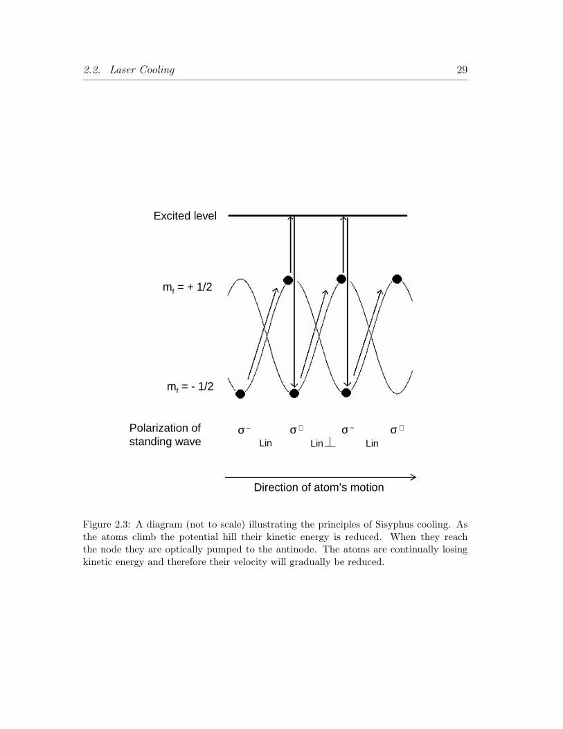
Linear ⊥ Linear Polarization Gradient Cooling
Two linearly polarized counter-propagating laser beams of the same frequency in-
terfere and create a strong polarization gradient. The polarization changes from
linear to σ+ in λ/4 (see Figure 2.3). If an atom absorbs a photon and is excited
then two outcomes are possible: the atom decays to the original level, or it decays
to a different magnetic sublevel. For the former case the atom receives a random
momentum kick but its energy does not change. For the latter case however, the
spontaneously emitted photon is of a higher frequency than the one that was ab-
sorbed (Figure 2.3). This means that the atom loses energy, leading to a reduction
in its velocity. By careful selection of the laser radiation detuning it is possible to
make it more probable for an atom to absorb a photon at the top of the ‘hill’ than
at the ‘bottom’. This leads to a reduction in the energy of the atoms i.e. cool-
ing. Figure 2.3 illustrates the principles of linear ⊥ linear polarization gradient
cooling.7
7Linear ⊥ linear polarization gradient cooling is also called Sisyphus cooling after the Greekmythological character, Sisyphus. He was doomed by the Greek gods to forever roll a largeboulder to the top of a hill.
2.2. Laser Cooling 29
Excited level
Polarization of standing wave
Direction of atom’s motion
mf = + 1/2
mf = - 1/2
LinLinσ + σ +σ −
Lin σ −
Figure 2.3: A diagram (not to scale) illustrating the principles of Sisyphus cooling. Asthe atoms climb the potential hill their kinetic energy is reduced. When they reachthe node they are optically pumped to the antinode. The atoms are continually losingkinetic energy and therefore their velocity will gradually be reduced.

2.2. Laser Cooling 30
σ+ − σ− Polarization Gradient Cooling
Two counter-propagating oppositely circularly polarized light beams create a light
field where the polarization is linear but rotates in direction about the beam’s axis.
When the atoms travel along the axis of the beams the light shifts of the ground
state sublevels remain constant and therefore Sisyphus cooling does not occur in
this case.
For a stationary atom the population distribution is symmetric across the mag-
netic sublevels and therefore the atom absorbs photons from both beams equally,
giving no net force on the atom. However, when the atoms are moving through a
polarization gradient, there is a difference in the scattering rate between the two
counter-propagating beams.8 Because the transition rate between different pairs
of magnetic sublevels of excited and ground states (Clebsch-Gordon coefficients)
depends on the orientation of the electron spin and the polarization of the laser
radiation driving the transition, an atom will preferentially absorb photons from
the laser beam which is opposing its motion if the laser radiation is red-detuned.
The distribution across the magnetic substates is no longer symmetric and there-
fore there is an imbalance in the absorption rate of photons from the two beams,
giving a force that opposes the atom’s motion.
Even though the sub-Doppler viscous force is much larger than the Doppler
viscous force, the temperature is still limited by heating caused by spontaneous
emission and fluctuations in the number of absorbed photons. Temperatures that
are a few times the recoil limit can be attained. The recoil temperature is given
by Tr = (hk)2
mkB. For caesium the recoil temperature is Tr = 197 nK.
Neither Doppler or sub-Doppler cooling contain a dependence on position,
therefore the atoms are not localized in space. The internal structure of atoms
can be used not only to cool them effectively, but also to confine them. In order
to trap atoms, magneto-optical traps were developed.
8Motion-induced orientation leads to an imbalance in the scattering from the two counter-propagating beams.

2.3. Magneto-Optical Traps 31
2.3 Magneto-Optical Traps
Most of the cooling in BEC experiments (in absolute terms) is performed in
magneto-optical traps (MOTs). Using light and magnetic fields it is possible to
confine a large number of atoms and cool them to temperatures less than 1 µK. The
first experimental demonstration of a MOT was in 1987 [66] and since then there
has been extensive treatment of MOTs in the literature [67, 68, 69, 70]. There are
many possible MOT orientations including the 4-beam MOT [71], the pyramidal
MOT [72], and the surface MOT [73].
A magnetic field is required in order to localize the atoms in space and it is
normally generated by a pair of anti-Helmholtz coils. The ground state and the
excited magnetic states are shifted in energy by the Zeeman effect. The excited
state has three Zeeman components (for a F = 1 state) and the transition frequency
of these states tune with magnetic field and therefore position. The atoms are
illuminated by two red-detuned (∆ < 0) counter-propagating beams of opposite
circular polarization. The imbalance in the forces of the two beams leads to a
resultant force on the atoms. A schematic of the principles of a MOT is given in
Figure 2.4.
2.3.1 Six-Beam MOT
Figure 2.4 illustrated the principles of a MOT in one dimension. To extend the
principle to three dimensions two further pairs of counter-propagating beams of
opposite circular polarization are added in orthogonal directions to the original
beams as illustrated in Figure 2.5.
The polarization configuration in a MOT implies that only σ+ − σ− polariza-
tion gradient cooling occurs. This would be true if the atoms only moved along
the axis of the beams. However, atoms move in random directions and therefore
at intermediate points between the axes the polarization is not well defined and
therefore both types of sub-Doppler cooling occur.

2.3. Magneto-Optical Traps 32
Energy
Position
Magnetic Field
F=0 Ground State
F=1 Excited State
mF= -1
mF= 0
mF= +1-1
0
+1
σ + σ −ω L
δ −
δ +
zz’
Figure 2.4: Arrangement for a MOT in one-dimension (1D). At point z = z′ the atomsare closer to resonance with the σ− beam. Therefore the atom is driven towards thecentre of the trap. Even though the scheme is described for F = 0 → F ′ = 1 transition,it works well for any F → F ′ = F + 1 transition. (σ+ and σ− denote transitions andshould be defined with respect to the direction of the magnetic field. However, in thiscase they are used to denote beams and are defined with respect to the z-axis.)
σ +
σ −σ −
σ −
σ +
σ +
I
I
Figure 2.5: Direction and polarization configuration of a six beam MOT.

2.3. Magneto-Optical Traps 33
B B
σ +
σ -
σ+
σ -
Figure 2.6: Cross-section of the pyramidal MOT and the resulting polarization configu-ration.
2.3.2 Pyramidal MOT
The pyramidal MOT is a way of generating the same radiation field as in a six-
beam MOT. A pyramidal MOT only requires one input beam to produce the same
configuration of light polarizations as a standard six-beam MOT. The original
pyramidal MOT consisted of a large beam of σ− polarized light incident on a
conical hollow mirror [72]. This was then modified to include a small hole at
the vertex in order to not only confine atoms but enable transfer of atoms into
the experimental MOT [74]. The first reflection on the mirror produces a pair
of counter-propagating beams with opposite polarization. The second reflection
then produces a σ+ retro-reflected beam. This occurs in all three dimensions
creating the required polarization configuration. Figure 2.6 illustrates the setup of
a pyramidal MOT.

2.4. Magnetic Trapping 34
2.4 Magnetic Trapping
Ions were first trapped and cooled in 1959 [75], but it took until 1985 to trap
neutral atoms [76]. Ions, which are trapped by the strong Coulomb interaction,
can be trapped from a background gas with no prior cooling. However, atoms
need to be cooled before loading them into a magnetic trap because of the shallow
depth of magnetic traps. Therefore the magnetic trapping of neutral atoms had
to wait until laser-cooling had been developed.
Neutral atoms are confined by the interaction of an inhomogeneous electromag-
netic field with the atomic dipole moment. The interaction between the magnetic
moment and the magnetic field produces a force given by the following equation:
F = ∇(µ.B) (2.4)
The potential energy of an atom with a magnetic moment is given by (in the limit
of a weak field):
U = −µ.B = mF gF µBB (2.5)
Earnshaw’s theorem states that local field maxima are not allowed.9 Therefore
in order to be able to trap neutral atoms, as the magnetic field increases the energy
of the atom must also increase. Atoms must therefore be in a low-field seeking state
i.e. mF gF > 0.
2.4.1 Zeeman Effect on the Hyperfine Ground States
The Zeeman energy of the two ground hyperfine states in the presence of a magnetic
field can be expressed by the Breit-Rabi equation [78]. The equation is given below
(Equation 2.6) and plotted for caesium in Figure 2.7.
Energy (J) = − hυHFS
2(2I + 1)− gIµBmF ± 1
2hυHFS ×
1 +
4mF
2I + 1x + x2
1/2
(2.6)
9Earnshaw’s theorem states: In a region devoid of charges and currents, the strength of aquasistatic electric or magnetic field can have local minima but not local maxima [77].

2.4. Magnetic Trapping 35
0 500 1000 1500 2000 2500 3000 3500 4000
−1
−0.8
−0.6
−0.4
−0.2
0
0.2
0.4
0.6
0.8
1
Breit−Rabi Equation
B−field(Gauss)
Ene
rgy/
hVhf
s
Figure 2.7: Zeeman effect of the hyperfine ground state for 133Cs.
where
x =(gJ + gI)µBB
hυHFS
The values for caesium of the gyromagnetic factors (gJ and gI), the hyperfine
splitting (νHFS) and the nuclear spin (I) are given in Table 2.1.
Name Symbol ValueGround State Hyperfine Splitting υHFS 9.192631770 ×10⁹ GHz
Nuclear Spin I 7/2Nuclear Gyromagnetic Ratio gI 0.00039885395Electron Gyromagnetic Ratio gJ 2.0023193043737
Planck’s Constant h 6.626069 ×10⁻³⁴ J sBohr magneton µB 9.274009 ×10⁻²⁸ J G−1
Table 2.1: Caesium-133 atomic structure constants required for the calculation of theBreit-Rabi equation.
2.4.2 Simple Magnetic Trap
The simplest magnetic trap was originally proposed by W. Paul and was exper-
imentally realized in 1985 [76]. It consists of two coils in an anti-Helmholtz ar-

2.4. Magnetic Trapping 36
A
I
I
R
Figure 2.8: Diagram of a simple magnetic trap. The dotted lines (· · ·) are the magneticfield lines. The distance 2A is the separation between the two coils. The black circleillustrates the position of the minimum of the magnetic field which is zero in this caseas the current in the coils is equal and opposite.
rangement. The magnetic field due to a circular coil at a point on its axis is given
by Equation 2.7.
Bz =µ0
2
nIR2
((A− z)2 + R2)32
(2.7)
where n is the number of turns, I is the magnitude of the current flowing through
the coil, R is the radius of coil and A is the distance along the axis of the coil from
the centre (see Figure 2.8). The field gradient for a pair of coils in anti-Helmholtz
arrangement with radius R and separation 2A is:
∂B
∂z
∣∣∣∣∣z=0
=3nIR2Aµ0
(A2 + R2)52
(2.8)
An inherent problem in this trap is the occurrence of a zero in the magnetic
field at the trap centre. This causes Majorana transitions (colloquially called “spin
flips”) when the atoms change their mF state leading to loss from the trap.
2.4.3 Majorana Transitions
In the presence of a magnetic field the atoms’ magnetic moment precess about
the field at the Larmor frequency: ωLarmor = mF gF µBB.10 In order to remain
10In the current experiment the magnetic field is rarely below 130 G and therefore the Larmorfrequency is always greater than 136 MHz.

2.4. Magnetic Trapping 37
trapped the atoms’ magnetic moment must follow the field adiabatically otherwise
the atoms undergo Majorana transitions [79] into un-trapped or anti-trapped states
(mF gF < 0). The rate of change of the field direction θ must be slower than the
precession of the magnetic moment:
dθ
dt<
µB|B|h
= ωLarmor
As long as dθ/dt is smaller than the trapping frequencies then there is negligible
probability of an atom undergoing a Majorana transition.
This problem prevented the early experiments from reaching BEC. This lead to
the development of a new generation of magnetic traps which avoided this problem
e.g. the TOP (time-averaged orbiting potential) trap [80] and the PLUG trap [2].
Another solution, is to use a Ioffe-Pritchard trap.
2.4.4 Ioffe-Pritchard Trap
A Ioffe-Pritchard (I-P) trap is formed by a linear quadrupole field and an axial
field. The linear quadrupole field is produced by 4 straight wires (Ioffe bars) par-
allel to the z-axis (Figure 2.9 (a) ), each carrying equal magnitude of current but
the direction of the current in each wire is opposite to its nearest neighbour (Fig-
ure 2.9 (b) ). The magnetic field along the z-axis is therefore zero. The axial field
is provided by two end coils (“pinch” coils) with current flowing in the same direc-
tion and with equal magnitude in both coils. This is illustrated in Figure 2.9 (a).
The “pinch” coils therefore add an axial magnetic field to the magnetic field pro-
duced by the Ioffe bars. This means that the field along the z-axis is no longer
zero and therefore there is negligible probability of an atom undergoing Majorana
transitions.
To calculate the magnetic field near the centre of the trap, consider four straight
wires, infinitely long and narrow, positioned perpendicular to the x-y plane and in
the positions and with current Ir flowing as indicated in Figure 2.9 (b). The field
produced by these wires provides radial confinement but has no component in the
z direction. The axial coils are n turn coils of radius R with current Ia flowing.

2.4. Magnetic Trapping 38
I I
+
.
(a) (b)
z axis c a x axis
y axis
A
+
.
R
Figure 2.9: A schematic of a Ioffe-Pritchard trap: (a) illustrates the physical arrangementof the bars and coils and the directions of the currents. Point c is the centre of themagnetic trap where x = y = z = 0, (b) illustrates the current direction in the Ioffebars.
The magnetic field produced by these two coils has no x or y component and as
long as the coils are separated by a distance greater than their radius they provide
axial confinement.
Combining the expressions for both the Ioffe bars and the “pinch” coils yields
the following expression:
B =
µ0Ir
2π
−y(x−a)2+y2 + y−a
(y−a)2+x2 + −y(x+a)2+y2 + y+a
(y+a)2+x2
x
µ0Ir
2π
x−a
(x−a)2+y2 + −x(y−a)2+x2 + x+a
(x+a)2+y2 + −x(y+a)2+x2
y
µ0nR2Ia
2
1
((A+z)2+R2)32
+ 1
((A−z)2+R2)32
z
(2.9)
The magnitude of the magnetic field can be determined by expanding Equa-
tion 2.9 around the origin (x = y = z = 0), keeping only the leading terms in the
expansion[81, 82].
B ∼= B0 +4µ0I
2r
π2a4B0
r2 +3B0(4A
2 −R2)
2(A2 + R2)2z2 , B0 =
µ0nR2Ia
(A2 + R2)32
(2.10)
where r2 = x2 + y2.
If µ is the magnetic moment of the atom then the energy of the atom in the
magnetic field can be written:
E = µB (2.11)

2.4. Magnetic Trapping 39
Substituting Equation 2.10 into the Equation 2.11 yields the following equation:
E = µB = µB0 +4µ0I
2r µ
π2a4B0
r2 +3B0(4A
2 −R2)µ
2(A2 + R2)2z2
= E0 +m
2(ω2
rr2 + ω2
zz2) (2.12)
Equating corresponding terms yields expressions for the trap frequencies of a Ioffe-
Pritchard trap as stated in Equation 2.13:
ωr =(
µ8µ0
mπ2
) 12 Ir
a2√
B0
and ωz =
(3µnR2µ0(4A
2 −R2)
m(A2 + R2)72
) 12 √
Ia (2.13)
The radial trap frequency is proportional to the current in the Ioffe bars and
inversely proportional to the square root of the bias magnetic field at the centre
of the trap. The axial frequency is directly proportional to the square root of the
current running through the coils.
There are many adaptations of the I-P trap, the most notable being the clover-
leaf trap developed at MIT [83] and the baseball trap developed at JILA [81].
2.4.5 Baseball Trap
A very convenient way to make an I-P trap is to bend the ends of the parallel wires
(Figure 2.9) into one coil. This creates a coil shaped like the seams on a baseball
(Figure 2.10). The ease of use of this trap arises from the fact that the four parallel
wires and “pinch” coils are now one ‘coil’. Therefore, applying a current to this
single coil effectively produces the same effect as equal current flowing through the
four parallel wires and the “pinch” coils. For the baseball coil, only one current
needs to be regulated, and therefore the need for complicated electronics is reduced.
The expression for the magnetic field for the Ioffe-Pritchard trap derived pre-
viously (Equation 2.9), is no longer accurate for the baseball trap. The expression
was calculated for four infinitely long and narrow wires and a pair of Helmholtz
coils, whereas the baseball coil is a single coil that provides both radial and axial
confinement. However, the magnetic field produced by the baseball coil is qualita-
tively similar to that in Equation 2.9.

2.4. Magnetic Trapping 40
Figure 2.10: Schematic of a baseball coil. The black circle illustrates the position of theminimum of the magnetic field.
Equation 2.9 becomes more inaccurate when gravity pulls the atoms down from
the centre of the trap. The expansion about the trap centre is no longer valid as
the atoms no longer sit at the centre of the coils. For a purely harmonic potential,
the amount of sag can be calculated by equating the force due to the potential to
the force due to gravity:
mω2zz = mg (2.14)
⇒ z =g
ω2z
(2.15)
For caesium atoms in a 12 Hz trap the magnitude of the sag is 1.7mm.
For atoms in a baseball trap, a minimum in the energy of the atoms (magnetic
and gravitational) still exists. Therefore, expanding the potential about the new
sagged trap centre yields leading terms that are quadratic. The smaller the spatial
size of the cloud the less important the anharmonic terms in the expansion are,
therefore the potentials can still be approximated as harmonic.
2.4.6 Experimental Considerations
Atoms cannot be loaded directly into a magnetic trap from room temperature
because of the small depth of the trap. This puts a constraint on the temperature
of the atoms to be loaded. Atoms are normally loaded into a magnetic trap from
a MOT or from optical molasses (temperatures in the µK range).
The shallow depth of neutral atom traps also puts constraints on the vacuum re-

2.5. Evaporative Cooling 41
quirements. A collision between a trapped atom and a thermal energy background
gas atom leads to the loss of the trapped atom from the magnetic trap. Therefore,
in order to produce condensates, low pressures must be attained and sustained in
the experimental cell. At low pressure, the trapping time is ≈ 10−8/P s where P
is the pressure in Torr [84].
2.5 Evaporative Cooling
Evaporative cooling was originally proposed by Hess in 1986 [85]. Experimental
demonstration soon followed in 1988 [86]. These evaporation experiments were
carried out on atomic hydrogen which had already been pre-cooled by cryogenic
methods. It was not until 1994 that the technique of evaporative cooling was ex-
tended to alkali metals by combining laser cooling and radio-frequency (rf) evap-
orative cooling [87, 88]. These experiments increased the PSD by six orders of
magnitude while only losing approximately a factor of a thousand atoms [1, 3].
Evaporative cooling is a highly efficient process as long as the rethermalization
time is significantly shorter than the lifetime of the atom cloud (see Chapter 4).
There are a number of ways of selectively removing hot atoms from the trap:
passing over a potential energy barrier [89], adsorption onto a pumping surface [90]
or by optical [91] or rf [92] pumping the atoms to non-trapped states. The most
common method in alkali metal experiments is radio-frequency (rf) evaporation.
2.5.1 Radio-Frequency Evaporation
Hot atoms have large orbits in the magnetic trap and therefore they span a large
range of magnetic field values. To address only the hot atoms a narrow magnetic
field or energy-sensitive transition is required, for example rf transitions between
adjacent Zeeman sublevels. By selecting the rf frequency carefully (and other
experimental parameters) the atoms can be induced to undergo an adiabatic tran-
sition from the trapped state directly to the anti-trapped state. The atoms are
thus expelled from the trap.
Rf evaporation has many advantages over other methods of evaporation. The

2.5. Evaporative Cooling 42
magnetic trap potential depth does not need to be lowered, and the evaporation
can be three-dimensional in velocity space as the atoms are evaporated from any
surface where the resonance condition is fulfilled. The rf surface removes all the
atoms whose energy is greater than the energy of the cloud by a fixed ratio η
and therefore the rf surface removes all atoms whose energy is greater than the
truncation energy given by εt = ηkBT . The larger the truncation energy the more
efficient the evaporation.11 The evaporation is however slower and therefore the
chosen experimental value of η is a balance between more efficient cooling and the
speed at which the cooling occurs.
At low-fields, the Breit-Rabi equation (Equation 2.6) simplifies to
E = gF mF µBB. The rf transitions between adjacent Zeeman sublevels (|∆mF|=1)
are therefore degenerate leading to multiphoton transition from a magnetically
trapped state to an un-trapped or anti-trapped state. However at high magnetic
fields the degeneracy is lifted. This is an important fact to consider for any ex-
periment evaporating at high magnetic fields. For 133Cs (3,−3) state at 500G,
the difference in the frequency of the rf transitions between mF = −3 ↔ −2 and
mF = −2 ↔ −1 transitions is of the order of 8MHz and this can lead to a decrease
in the efficiency of evaporation [93].
2.5.2 Effects of Gravity on Evaporation
To support the atoms against gravity a magnetic field gradient is required. The
force in the z-direction due to the trap is equated to the force on the atoms due
to gravity.
Fz = gF mF µB∂B
∂z= mg (2.16)
The minimum gradient for the 133Cs F = 3, mF states 3, 2, and 1 is 31.3, 47.0 and
94.0G cm−1 respectively. Under normal conditions all three magnetically trappable
states are supported in the magnetic trap. However, the presence of many states in
the magnetic trap increases the probability of inelastic collisions leading to losses
from the trap. To reduce the presence in the magnetic trap of all states except
11This is only true in the absence of any loss or heating in the atom cloud.

2.5. Evaporative Cooling 43
(a) (b) (c)
Front view Top view Side view
z
y
x
y
z
x
Figure 2.11: The effect of gravity on the magnetic potential. The coloured contour linesare the potential that the atoms experience (including gravity). The black ellipse is therf evaporation surface. This clearly shows that gravity does indeed make the evaporationone-dimensional.
F = 3, mF = −3 , the atoms can either be optically pumped into the (3,−3)
state or the magnetic trap gradient reduced so that other mF states are no longer
supported against gravity. Also, after loading it is possible to expel the (3,−2)
and (3,−1) atoms from trap using a radio-frequency cutting surface.
How does gravity affect the simple picture?
In a zero gravity environment, the cloud of atoms sits perfectly centred on
the B-field contours. The evaporation surface determined by the rf frequency
then touches the extremity of the cloud in all directions, resulting in efficient 3D
evaporation. In reality, gravity pulls the cloud downwards leading to an offset
in the centre of the cloud from the centre of the magnetic trap. As calculated
previously, for weak traps with vertical trapping frequencies of the order of 10Hz,
the sag is over 2 mm (Equation 2.15). The bottom of the cloud experiences a
higher magnetic field than the top. Consequently the evaporation surface is only
in contact with one side of the cloud, leading to one dimensional evaporation. This
is illustrated in Figure 2.11.
There is one benefit of 1D evaporation. Gravity puts the atoms into a region
where the rf contours vary much more quickly across the cloud. This enables
precise cutting – a cutting surface which is shallower and less susceptible to stray

2.5. Evaporative Cooling 44
magnetic fields.
2.5.3 Dimensionality of Evaporation
When evaporation is three-dimensional all the atoms with energy greater than
ηkBT are removed from the trap. Evaporation is one-dimensional when Ez > ηkBT
and two-dimensional when Ex + Ey > ηkBT . These criterion only apply when the
magnetic trapping potential is separable. If the rate of mixing between potentials
is faster than the rate of elastic collisions then the evaporation is always three-
dimensional.
Evaporation in lower dimensions leads to a reduction in the efficiency [94]
because atoms with an energy higher than the truncation energy may undergo
many collisions before leaving the magnetic trapping potential. In the absence of
inelastic collisions, the dimensionality of the evaporation surface does not affect the
efficiency of the evaporation, it only leads to longer evaporation times. However,
in the presence of inelastic collisions a time limit is set on the evaporation process
and therefore dimensionality of the evaporation process has a dramatic effect on
the efficiency.
In a magnetic trapping potential the frequency of the rf is given by:
hωrf = ∆mF gF µBB (2.17)
= gF µBB (as ∆mF = 1) (2.18)
If the atom cloud sits perfectly centred on the magnetic trapping contours then
|B|=constant contours are equipotential surfaces and therefore the rf surface drives
transitions into un-trapped and anti-trapped states at positions of equal ηkBT in
all three dimensions.
When the truncation energy is set as ηkBT the average energy of the atoms
removed is not necessarily εt. To account for the slight difference an extra factor κ
is introduced. Therefore, the average energy of atoms removed from the trapping
potential is:
ε = (η + κ)kBT (2.19)

2.5. Evaporative Cooling 45
The value of κ is normally between 0 and 2 and can be neglected for large values of
η. Evaporated atoms have an average excess energy of κkBT . If the gravitational
energy across the equipotential surface U = ηkBT varies by ±kBT then evaporation
only occurs at the bottom of the cloud.
For harmonic confinement along the z-axis:
U =U ′′z2
2(2.20)
The equipotential surface therefore exists at:
z ≈√
2ηkBT
U ′′ (2.21)
Evaporative cooling becomes one-dimensional when:
kBT <2η(mg)2
U ′′ (2.22)
<2ηmg2
ω2z
(2.23)
For caesium atoms in a 10 Hz trap the evaporation becomes one-dimensional
(for η = 6) when the temperature falls below approximately 5mK. The tempera-
ture achieved in optical molasses is of the order of tens of µK and therefore in weak
magnetic traps the evaporation is always one-dimensional. The dimensionality of
the evaporation can be increased by operating in tighter magnetic traps.12
12Gravitational sag still exists in tighter traps but the difference in energy across the cloud isless than kBT .
Chapter 3
Scattering Theory and FeshbachResonances
Inter-atomic collisions are crucial for evaporative cooling: atom clouds rethermal-
ize through elastic collisions; trap heating and loss occur due to inelastic collisions.
Evaporation performance depends on the ratio between elastic and inelastic col-
lisions (Chapter 4) and therefore understanding inter-atomic collisions and their
dependence on external parameters can mean the difference between succeeding
and failing to create a BEC.
3.1 Atomic Interactions
The interactions between the two colliding atoms can have significant effect even
when the atoms are far apart (compared to the radii of the electronic charge
clouds). We can write the Hamiltonian for two interacting atoms as:
H(r, s) = H0(r) + H12(r, s) (3.1)
where H0(r) and H12(r, s) are the unperturbed and interaction Hamiltonian respec-
tively. The inter-atomic separation between the two colliding atoms is denoted by
r (= R1 −R2) and their spin by s.
The unperturbed Hamiltonian describes non-interacting atoms in a magnetic
trapping potential. Equation 3.1 is valid when the atoms can be treated individu-
ally and the interactions as a perturbation. The interaction Hamiltonian is given
46

3.1. Atomic Interactions 47
by:
H12(r, s) = Hv(r) + Hex(r, s) + Hd(r, s) (3.2)
where Hv(r), Hex(r, s) and Hd(r, s) are the Hamiltonians representing the van der
Waals, exchange term and dipolar interactions respectively.
For the previous equations (Equations 3.1 and 3.2) the terms in brackets fol-
lowing each individual Hamiltonian give the dependence of the corresponding in-
teraction on r and s. If the interaction depends on r, then changes in the external
degrees of freedom can occur. Equivalently, if the interaction depends on the spin,
then changes in the internal state of the colliding atoms can occur.1
3.1.1 Unperturbed Hamiltonian
The unperturbed Hamiltonian H0, of two colliding atoms is the Hamiltonian of
two separate non-interacting atoms in a magnetic field. Equation 3.3 states the
terms that are included in the unperturbed Hamiltonian.
H0(r) = − h2
2µ∇2 + Hh + HZ (3.3)
The first term is associated with the kinetic energy (µ = m/2 where m is the
reduced mass), and Hh and HZ are the Hamiltonians for the hyperfine interaction
and the Zeeman interaction respectively.
3.1.2 van der Waals Interaction and Exchange Terms
The two main interactions for two colliding neutral atoms are the van der Waals
interaction and exchange interaction.
The van der Waals interaction Hv(r), arises from the induced electric dipoles
and quadrupoles of the neutral atoms2 and can be written in the form:
Hv(r) = −C6r−6 − C8r
−8 − C10r−10 + . . . (3.4)
1A change in the internal states of the colliding atoms is synonymous to a change of channeloccurring during a collision. Prior to colliding the atoms are in the entrance channel, followingthe collision they are in the exit channel. If the entrance and exit channels are the same/differentthen an elastic/inelastic collision has occurred.
2All permanent electric dipoles and multipoles are absent in a ground state neutral atom.

3.1. Atomic Interactions 48
1094 8765
3u
Ener
gy
Interatomic Separation (A)
1 +g
Figure 3.1: Schematic of the interaction potentials as functions of the inter-atomicseparation for two ground state caesium atoms with electrons in singlet X1 ∑+
g andtriplet a3 ∑
u states. The exchange interaction causes a splitting in energy depending onwhether the spins of the colliding atoms are parallel (S = 1 or triplet) or anti-parallel(S = 0 or singlet).
At large inter-atomic separation the van der Waals interaction is due to the in-
duced dipole-dipole interaction between the atoms which is caused by their in-
dividual electron charge distributions creating small instantaneous dipoles. The
Hamiltonian can be approximated by:
Hv(r) ≈ −C6r−6 (3.5)
As the van der Waals interaction is spin independent no transitions between
internal states can occur. However, the exchange interaction is spin dependent and
can couple the singlet and triplet parts of the wavefunction leading to changes in
the internal state of the colliding atoms.
The exchange interaction occurs when the electron clouds of two colliding atoms
overlap. The individual spins of the electrons (S1 and S2) decouple from the nuclear
spins and recombine to form molecular electronic spin states:
S = S1 + S2

3.1. Atomic Interactions 49
Similarly the nuclear spins combine to form molecular nuclear spin states:
I = I1 + I2
Therefore the total F and mF are conserved:
F = S + I
and
mF = mF1 + mF2
The exchange interaction arises from the anti-symmetry of the electronic wave-
function of the two colliding atoms. At small inter-atomic separation the wave-
functions of the electrons overlap and there is a contribution to the energy of the
resulting potential depending on the orientation of the valence electron spins. If
the spins are anti-parallel (S = S1 + S2 = 0) then the two electrons can occupy
the same orbital3 giving rise to a singlet potential. When the two electron spins
are parallel (S = S1 + S2 = 1) their spin wavefunction is identical and therefore
they cannot have the same spatial wavefunction. Therefore, due to the electron
repulsion there is no reduction in the energy of the potential at short range. The
potential therefore splits into two – singlet and triplet. They have corresponding
scattering lengths denoted by aT (triplet) and aS (singlet). Figure 3.1 illustrates
the splitting in the potential at short inter-atomic separation, that arises due to
the exchange interaction. For most collisions the interaction potential is a mixture
of the triplet and singlet potential. The exception to this rule is collisions be-
tween two atoms in the (4, 4) state and the collisions between atoms in the (4, +4)
and (4, +3) state. For these collisions the interaction potential is purely triplet in
nature.
For the exchange interaction, the inelastic loss rate coefficient for laser-cooled
alkali metals is of the order 10−10 cm3 s−1 [48]. Therefore to avoid these losses,
atoms are polarized into the |F = I ± S, mF = ±F > states.4
3The overlap of the electronic wavefunctions of two atoms with anti-parallel valence electronspins leads to a formation of a covalent bond between the atoms.
4For caesium, these states are |F = 4, mF = ±4 > and |F = 3, mF = ±3 >.

3.1. Atomic Interactions 50
The potential energy curves (Figure 3.1) can be broken into three distinct re-
gions. At small inter-atomic separation (r ≤ 5a0) the interactions are dominated
by the strong repulsive core due to the overlapping of electron clouds. At inter-
mediate r, the exchange interaction is dominant and splitting of the potential into
singlet and triplet parts occur. At large r (r ≥ 20a0) the magnitude of the split-
ting between the triplet and singlet potentials is reduced and the van der Waals
interaction dominates. These effects are shown clearly in Figure 3.1.
The van der Waals energy and the exchange energy can be viewed as the
mean energy or half the energy difference between the singlet and triplet potential,
respectively:
Vv(r) =1
2(VS=0(r) + VS=1(r)) (3.6)
Vex(r) =1
2(VS=0(r)− VS=1(r)) (3.7)
3.1.3 Dipolar Interaction
Losses from a magnetic trap due to the exchange interaction can be prevented by
polarizing the trapped atoms into stretched states. Other weaker interactions can
couple the stretched states to other internal states thus causing heating and loss
from the trap. The most dominant interactions of this type are due to the dipolar
interaction, Hd. This interaction occurs between the spin of the two colliding atoms
and can be split into two main types: the direct magnetic dipole interaction (spin-
spin dipole interaction) and the second-order spin-orbit interaction (or indirect
spin-spin coupling). The complete Hamiltonian for dipolar relaxation is a sum
of the spin-spin dipole interaction Hamiltonian and the second-order spin-orbit
interaction Hamiltonian:
Hd = H1d + H2
d (3.8)
where H1d and H2
d are given by the following expressions:
H1d = V1(r)VS(S1, S2) (3.9)
H2d = V2(r)VS(S1, S2) (3.10)

3.1. Atomic Interactions 51
The spins of the atoms are coupled individually to the inter-atomic axis, there-
fore VS commutes with the individual spins (S1, S2) and not the total spin (S).
The orbital angular momentum quantum number (l), can therefore change by +2,
0, or −2. It is possible for two incoming atoms in an s-wave state (l = 0) to scat-
ter into a d-wave state (l = 2). The extra angular momentum required is taken
from the electronic spins. If the Zeeman energy released from the collision is small
compared to the energy required to impart the angular momentum to the colliding
atoms, then these inelastic collisions are suppressed.5 This suppression takes the
form of a centrifugal term in the interaction Hamiltonian.
The spin-spin dipole interaction is due to the coupling between the magnetic
dipole associated with the spin of one atom, with the magnetic field produced by
the magnetic dipole of the colliding atom. The interaction lifts the degeneracy of
the different electronic spin projections of the triplet state.
The second-order spin-orbit interaction creates the same effect as the spin-
spin dipole interaction in that the degeneracy of the triplet state is lifted. When
the electron clouds of the interacting atoms overlap, off-resonant coupling of the
electronic wavefunctions to higher-lying electronic states can occur.
The observed effects from spin-spin dipole interaction and the second-order
spin-orbit interaction are indistinguishable. The dipolar relaxation rate coefficient
for most alkali metals is of the order 10−15 cm3 s−1 [48]. The spin-spin dipole inter-
action occurs in all collisions involving alkali metal atoms and is primarily responsi-
ble for dipolar relaxation observed in hydrogen and the lighter alkali metals. How-
ever, the dipolar relaxation rate coefficient for Cs is of the order 10−12 cm3 s−1 [24].
This large rate is attributed to the second-order spin-orbit interaction that occurs
in collisions involving heavy alkali metals with large relativistic spin-orbit effects
e.g. Cs and Rb. For 87Rb, the effect of the spin-spin dipole and the second-order
spin-orbit interactions are approximately equal and opposite, giving an anoma-
lously small dipolar relaxation rate [48].
5To take advantage of the suppression of these collisions, experimentalists use very low mag-netic fields (see Section 1.2.2, Chapter 2).

3.2. Scattering 52
3.2 Scattering
Different quantum mechanical approaches are appropriate for studying scattering
problems in different energy regimes: the Born approximation – high energy, and
partial wave analysis – low energy.
In the Born approximation the energy eigenfunctions of the system are ex-
pressed as a linear combination of the incident and scattered waves. The effect of
the interaction is treated as a weak perturbation and therefore the Born approx-
imation method is only valid when the average energy of the interaction between
the incident particle and the scatterer is much smaller than the incident particle’s
kinetic energy.
In partial wave analysis the incident plane wave is expressed as a linear com-
bination of the eigenfunctions of the scattering potential. This method is useful
in describing the scattering of plane waves from spherical objects. No limitations
are placed on the strength of the interactions. This is the method most commonly
used to describe inter-atomic scattering.
3.2.1 Partial Wave Analysis
The interaction Hamiltonian of two colliding structureless particles is:
H = − h2
2µr2
d
dr
(r2 d
dr
)+
h2l(l + 1)
2µr2+ V (r) (3.11)
where µ and r are the reduced mass and the inter-atomic separation of the two
interacting particles, respectively.
At small inter-atomic separation (r) the interaction potential V (r), is of the
order of the total energy and therefore the solutions are complicated. At large r,
the magnitude of V (r) is small and the wavefunctions tend towards the solutions of
the general Schrodinger equation in the absence of the interaction potential term.
In the asymptotic region (large r) the interaction Hamiltonian has solution of the
form:
ψl(r) ∼ sin [kr + δl(k)]
r(3.12)

3.2. Scattering 53
where k is the deBroglie wave vector and is given by:
k =
(16mkBT
πh2
) 12
(3.13)
δl is called the phase shift and is known to reflect the effect of the potential on the
scattered wave (see Reference [95]). The phase shifts cannot be directly measured,
however they are related to the collision cross-section (which is experimentally
measurable) by the following equation:
σ =4π
k2
∞∑
l=0
(2l + 1)sin2δl (3.14)
where k =√
2µE/h and the sum is over all possible partial waves with angular
momentum l.
Symmetry requirements affect the partial waves allowed in collisions involving
identical particles. For fermions, s-wave collisions are forbidden because of the
Pauli exclusion principle which states that atoms cannot have the same spatial
and spin wavefunctions. Therefore only odd l-wave collisions occur (p-wave, f -
wave, etc). For bosons, only partial waves of even l (s-wave, d-wave, etc) are
allowed because of the symmetry of the wavefunction.
Hard Sphere Scattering
Consider a potential of the form:
V (r) =
0 r > a∞ r ≤ a
(3.15)
Figure 3.2 illustrates the form of the potential and the incident and scattered
waves.6 The incident wavefunction is continuous at the origin (r = 0) and the
scattered wavefunction is continuous at r = a. The phase shift is therefore pro-
portional to a. This illustrates why scattering from a potential can be compared
to hard sphere scattering.
For s-wave scattering (ka ¿ 1), the phase shift between the incident and
scattered wavefunction is ka. The total cross-section is obtained by substituting
6This is an over simplification of scattering, but it is useful for understanding the physicalorigin of the phase shift.

3.2. Scattering 54
a
V
Interatomic Separation
Figure 3.2: Scattering from a hard sphere potential. The dotted line (· · ·) is the incidentwave and the solid line (–) is the scattered wave.
this value into Equation 3.14 to give:
σ =4π
k2sin2(−ka) ≈ 4πa2 (3.16)
The geometrical cross-section is πa2, therefore the scattering cross-section is a
factor of 4 larger.
3.2.2 Scattering Length
Ground state collisions can be described by one parameter, the scattering length
a. The scattering length can be thought of as the radius of a hard sphere that
would produce the same scattered wavefunction as scattering from an inter-atomic
potential.7
The Wigner threshold laws state that for low enough energies, the phase shift δ0
is inversely proportional to the wavevector k of the atom motion. The expression
for the scattering length is given by:
a = − limk→0
δ0
k(3.17)
The scattering length characterizes the strength of the interactions and there-
fore can be negative, zero, or positive. Figure 3.3 illustrates schematically how
7In Figure 3.2 the scattering length is a.

3.2. Scattering 55
0.0 0.2 0.4 0.6 0.8 1.0 1.2 1.4
0.0 0.2 0.4 0.6 0.8 1.0 1.2 1.4
-0.2 0.0 0.2 0.4 0.6 0.8 1.0 1.2 1.4
r / r0 r / r
0
r / r0
(a)
(b) (c)
Figure 3.3: Schematic behaviour of the wavefunctions of the colliding atoms. The curvesin (a), (b) and (c) correspond to zero, positive and negative scattering lengths respec-tively. χ is the radial wavefunction multiplied by r. (The wavefunction equation used togenerate the plots was obtained from Reference [96].)
these changes in the scattering length arise.
3.2.3 Scattering at Low Temperatures
The number of partial waves involved in a collision depends on the energy of the
colliding particles. The only partial waves that contribute to the cross-section are
those which satisfy the following condition:
ka >√
l(l + 1) (3.18)
where a is the scattering length.
For low temperatures ka ¿ 1, and therefore only the l = 0 partial waves
(s-waves) contribute to the scattering cross-section. Equation 3.14 simplifies to:
σ =4π
k2sin2δ0 (3.19)
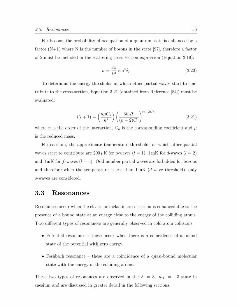
3.3. Resonances 56
For bosons, the probability of occupation of a quantum state is enhanced by a
factor (N+1) where N is the number of bosons in the state [97], therefore a factor
of 2 must be included in the scattering cross-section expression (Equation 3.19):
σ =8π
k2sin2δ0 (3.20)
To determine the energy thresholds at which other partial waves start to con-
tribute to the cross-section, Equation 3.21 (obtained from Reference [84]) must be
evaluated:
l(l + 1) =(
nµCn
h2
) (3kBT
(n− 2)Cn
)(n−2)/n
(3.21)
where n is the order of the interaction, Cn is the corresponding coefficient and µ
is the reduced mass.
For caesium, the approximate temperature thresholds at which other partial
waves start to contribute are 200µK for p-waves (l = 1), 1 mK for d-waves (l = 2)
and 3mK for f -waves (l = 5). Odd number partial waves are forbidden for bosons
and therefore when the temperature is less than 1mK (d-wave threshold), only
s-waves are considered.
3.3 Resonances
Resonances occur when the elastic or inelastic cross-section is enhanced due to the
presence of a bound state at an energy close to the energy of the colliding atoms.
Two different types of resonances are generally observed in cold-atom collisions:
• Potential resonance – these occur when there is a coincidence of a bound
state of the potential with zero energy.
• Feshbach resonance – these are a coincidence of a quasi-bound molecular
state with the energy of the colliding atoms.
These two types of resonances are observed in the F = 3, mF = −3 state in
caesium and are discussed in greater detail in the following sections.

3.3. Resonances 57
3.3.1 Potential Resonances
An inter-atomic potential can support many bound states, particularly if the po-
tential is deep. During scattering, the energy of the entrance channel is greater
than the dissociation energy (zero-energy) of the molecular state and therefore the
existence of bound states has no effect on the scattering.8 However, when the last
bound state9 of the molecular potential is close to the energy of the scattering
channel potential and the energy of incidence of the two scattering particles is
small (ka ¿ 1), resonances in the scattering cross-section occur.
If the depth of the potential is increased then more bound states can be sup-
ported. As each extra bound state that is added to the potential passes through the
zero of energy, a resonance occurs. The phase shift of the wavefunction increases
by π across the resonance and the width of the resonance becomes narrower as the
depth of the the potential increases. The scattering length also becomes very large
and goes through infinity on passing through each resonance.
Immediately prior to each resonance the total phase shift10 is an integer multiple
of π and therefore the cross-section is zero.11 The scattered wave is in phase with
the incident wave and therefore the particles do not collide, they pass through one
another.
On resonance, the phase-shift is equal to π/2 and Equation 3.20 and therefore
the cross-section takes it maximum value:
σ =8π
k2(3.22)
This is known as the unitarity limit, and in this limit the cross-section is orders of
magnitude greater than the off-resonance value. This increases the probability of
collisions in an atom cloud.
8Strictly speaking, in quantum mechanical treatment of scattering, all bound states must beincluded in the complete Hamiltonian.
9When l 6= 0 the potential can support quasibound states above the dissociation threshold.These give rise to what is known as shape resonances which behave like Feshbach resonances.
10Levinson’s theorem [98] states that the total phase shift is directly related to the number ofbound states in the potential.
11This is known as the Ramsauer-Townsend effect and was first observed in 1921 [99, 100].

3.3. Resonances 58
0.0 0.5 1.0 1.5 2.0 2.5 3.0
Potential Depth, ka/ (dimensionless)
Phas
e Sh
ift
/k2
- /2
/2
0
Cro
ss-S
ectio
n
0
Figure 3.4: The effect of the depth of the potential on the collisional cross-section andthe phase-shift.
When the last bound state is very close to the dissociation limit (i.e. the
scattering length is large but not equal to infinity) the first order approximation
of the cross-section is:
σ =8πa2
1 + k2a2(3.23)
which reduces to Equation 3.22 when ka À 1. At low temperatures (ka ¿ 1):
σ = 8πa2
The extra factor of 2 compared to the hard sphere scattering cross-section result
(Equation 3.16) arises from the indistinguishability of bosons.
These potential resonances have been observed in Cs in both singlet and triplet
potentials. The existence of these resonances can partially explain why Cs exhibits
dramatically different behaviour to other lighter alkalis. It also explains the energy
dependence of the low-temperature elastic cross-section [25].

3.3. Resonances 59
3.3.2 Feshbach Resonances
Feshbach resonances occur when the total energy of the entrance channel matches
the energy of a bound state in a closed channel. The incident particles “virtually”
occupy the bound state for a brief period of time and therefore spend an increased
amount of time at short range than they would normally. This causes a resonant
change in the elastic and inelastic cross-sections (or equivalently the scattering
length). The smaller the difference between the energy of the atoms in the exit
and entrance channels the larger the changes in the collisional cross-section. The
sign of the scattering length also depends on the position of the bound state relative
to the energy of the entrance channel. If the energy of the bound state is greater
than the energy of the entrance channel then the scattering length is negative i.e.
the interaction is attractive.
The energies of the bound states in the potential depend on external parameters
including magnetic field. The magnetic field dependence of the energy of the bound
state is in general different to the dependence of the energy of the binary scattering
state on magnetic field. Therefore both the magnitude and the sign of the effective
atom-atom interactions can be tuned.
Figure 3.5 illustrates schematically the principles of a Feshbach resonance. In
elastic scattering, the colliding atoms enter and exit the potential in the same
channel. In an elastic Feshbach resonance this is still true except this time there
is a delay introduced in the outgoing wave which is equivalent to a change in
the phase shift. As seen previously (Equation 3.14) this leads to a change in
the collisional cross-section. In inelastic scattering, the outgoing channel is lower
in energy than the entrance channel and atoms change channel because of non-
adiabatic transitions that occur at short-range curve crossings. In an inelastic
Feshbach resonance the inelastic cross-section also changes due to the increased
time the atoms spend at short range.
The width of a Feshbach resonance depends on the coupling between the en-
trance and exit channels. Therefore, unlike as in the case for potential resonances,
there is no limit to the width of a resonance.

3.3. Resonances 60
Interatomic Separation
non-adiabatic transition
(b)
Eres
E0
E0
Ener
gyEn
ergy
(a)
Figure 3.5: A plot of the potential energy curves for two different channels that illustratethe formation of Feshbach resonances. Eres is the energy of a state in a closed channeland E0 is the threshold energy for the entrance channel. In (a), the phase shift ofthe outgoing wave with respect to the incident wave causes a resonant alteration of theelastic cross-section. In (b) inelastic collisions are strongly enhanced due to the existenceof an avoided crossing between the entrance channel and a lower-lying outgoing channel.(Figure modified from Reference [101].)

3.3. Resonances 61
Feshbach resonances have been observed in many alkali metal experiments –
23Na [16], 85Rb [102], 87Rb [103], 6Li [104, 105], 133Cs [38] and 40K [106].

Chapter 4
Evaporative Cooling
The technique of forced evaporation has been very successful in many experi-
ments involving trapped alkali metal atoms. This technique involves driving radio-
frequency (rf) transitions that selectively remove the hottest atoms from the trap.
Typically atoms with energies greater than ηkBT (η ≈ 5) are removed from a trap
containing a cloud of atoms at temperature T and the cloud then rethermalizes
through elastic collisions to a lower temperature. The Maxwell-Boltzmann distri-
bution is therefore continuously truncated at a value of ηkBT and the high energy
tail of the distribution is continually replenished through elastic collisions. The
rate of evaporative cooling is determined by how rapidly the sample rethermal-
izes through elastic collisions. Additionally, the rate of the inelastic loss processes
impacts on the efficiency of the cooling process.
Evaporative cooling is crucial to attain BEC and has been studied in detail [107,
108, 109, 110]. An excellent review article on evaporative cooling is Reference [111].
Prior to constructing a BEC experiment it is important to consider the factors
that affect the evaporation.1 The choice of magnetic field and trapping frequencies
strongly affect the evaporation performance and therefore these factors need to be
considered not only when evaporating but also before construction of the magnetic
trap. The choice of magnetic trap depends on the trapping frequencies required and
1This is particularly true for elements that are difficult to condense e.g. 85Rb and Cs.
62

4.1. Elastic and Inelastic Collisions 63
the range of magnetic fields that need to be accessed. This chapter is a discussion
of the factors that affect the evaporation performance.
4.1 Elastic and Inelastic Collisions
The efficiency of evaporative cooling depends on the elastic collision rate and the
loss and heating rates due to inelastic collisions. To decide on an evaporation
strategy the dependence of these rates on magnetic field and trap frequencies must
be considered.
4.1.1 Elastic Collisions
Elastic collisions are required to rethermalize the cloud of atoms. The elastic
collision rate is given by the following equation:
Γelastic =< n > σ < vrel > (4.1)
where < n > is the mean density and σ is the elastic collision cross-section:
σ =8πa2
1 + k2a2(4.2)
k is the deBroglie wave vector and is defined in Equation 3.13, Chapter 3. vrel is
the average relative speed of the atoms in a trap given by the following equation:
< vrel >=
(16kBT
mπ
) 12
(4.3)
4.1.2 Inelastic Collisions
The efficiency of evaporation does not just depend on elastic collisions but also on
loss processes. A low elastic collision rate by itself is not necessarily a problem.
However, there is another timescale of importance, namely the lifetime of an atom
in the magnetic trap. Three processes contribute to losses in the magnetic trap:
1. Background collisions (loss rate=1/τb). Indiscriminate collisions between
cold trapped atoms and room temperature atoms in the background gas give
a loss rate per atom that is only dependent upon the vapour pressure of the

4.1. Elastic and Inelastic Collisions 64
background gas. The loss rate from this process equals 1/τb where τb is the
lifetime in the trap at a density low enough that the density dependent losses
can be ignored. The average mean energy of an atom lost from the trap due
to background collisions is 3kBT .
2. Two-body collisions – dipole relaxation (rate constant, K2). These inelastic
collisions occur between two trapped atoms, in which the two atoms exchange
angular momentum between their orbital motion and their intrinsic spin,
thereby scattering into un-trapped spin states. These collisions result from
both the direct magnetic dipole-dipole interaction and the indirect second-
order spin-orbit interaction. As the loss rate is proportional to the density,
the atoms lost from the trap have a lower than average energy, E2 = 94kBT .
3. Three-body collisions – molecule formation (rate constant, K3). Three atoms
collide in such a way that two form a molecule, whilst the third atom is nec-
essary to conserve energy and momentum. This process becomes significant
at high densities. The mean energy of an atom lost from the trap due to
three-body collisions is, E3 = 2kBT .
The last two processes are density dependent, therefore atoms are preferentially
lost from the the cold dense centre of the trap, resulting in an additional heating
of the sample (anti-evaporation). For a magnetically trapped gas containing N
atoms, the total loss rate is:
Γ =dN
dt= −N
τb
−K2 < n > N −K3 < n2 > N (4.4)
where
< n >=1
N
∫n2(r)d3r
and for a Gaussian distribution,
< n2 >=1
N
∫n3(r)d3r =
8√27
< n >2

4.2. Efficiency of Evaporation 65
4.2 Efficiency of Evaporation
The efficiency of the evaporative cooling process is determined by the ratio R of
elastic (good) to inelastic (bad) collisions. Any evaporation strategy must max-
imize this ratio. For efficient ‘runaway’ evaporation, R is typically greater than
100.2 In many experiments the technique of adiabatic compression is employed
to increase the initial elastic collision rate in the gas while maintaining the phase
space density.
For a change in trap frequencies to be considered adiabatic [112] the following
criteria must be satisfied:dω
dt¿ ω2, Γ2
elastic
During an adiabatic compression the entropy and thus the PSD is conserved.
The peak density npk is proportional to ω3/T 3/2 where ω3 = ω2rωz. The average
velocity is proportional to T 1/2 and therefore, if we assume that the elastic cross-
section is independent of the temperature, Equation 4.1 gives:
Γelastic ∝ ω3
T(4.5)
During adiabatic compression w/T is fixed and therefore the elastic collision rate
is:
Γelastic ∝ ω2 (4.6)
At finite temperatures, the collision cross-section is described by Equation 4.2.
At high temperatures ka À 1, the elastic collision cross-section reduces to:
σ =8π
k2∝ 1
T
Therefore, the dependence of the elastic collision rate on the trap frequencies is
reduced to:
Γ′elastic ∝ ω (4.7)
To determine the threshold for ‘high temperature’ behaviour, we can set ka
equal to 1. This gives an equation for the threshold temperature in terms of the
2This factor is much higher if inelastic collisions in addition to background collisions areconsidered. This factor is also affected by the geometry of the magnetic trap.

4.2. Efficiency of Evaporation 66
mass m, h, kB, and the scattering length a.
T =πh2
16mkBa2(4.8)
For a scattering length of 2525 a0, the temperature threshold at which low tem-
perature behaviour is observed is 40 nK. Therefore in order to benefit from large
scattering lengths the cloud must be cooled significantly.
At first glance, Equations 4.6 and 4.7 suggest that a tighter trap would be
beneficial. Not only is there an increase in the elastic collision rate (Equation 4.6)
but the problem of gravity which is inherent in weak traps is avoided (Section 2.5.2,
Chapter 2) and the BEC transition temperature is higher
kBTc = 0.94hωN13 where ω = (ω2
rωz)13 (4.9)
which means that the absolute heating rate is less important.
However, on analysis of the inelastic scattering rates, adiabatic compression
does not appear to be advantageous. Consider three scenarios:
1. If the loss rates are dominated by background collisions. Background col-
lisions are independent of trap frequencies therefore the optimum value of
the ratio of elastic to inelastic collisions R, is also the optimum value of the
elastic collision rate, Γelastic.
2. If the loss rates are dominated by three-body collisions:
R =Γelastic
Γ3−body
=6√
3πσk2BT 2
Nω3m2K3
∝ σ
ω(4.10)
If the elastic collisional cross-section is independent of temperature then
R ∝ 1
ω
However, if the elastic cross-section is proportional to 1/T then
R′ ∝ 1
ω2
Increasing the trap frequencies therefore makes the ratio of good to bad
collisions worse.

4.2. Efficiency of Evaporation 67
3. If the loss rates are dominated by two-body collisions:
R =Γelastic
Γ2−body
=4σ
K2
√kBT
πm∝ ω
12 (4.11)
If the elastic collisional cross-section is independent of temperature then
R ∝ ω12
As the temperature is decreased the value of R decreases, leading to a reduc-
tion in the efficiency of the evaporation. If the trap frequencies are increased
then the ratio of elastic to inelastic collisions should improve. However, if
the elastic cross-section is proportional to 1/T then
R′ ∝ 1
ω12
Once again, increasing the trap frequencies makes the evaporation less effi-
cient.
Any evaporation strategy maximizes the ratio of elastic to inelastic collisions
and hence it must take into account which of the loss mechanisms is dominant.
The technique of adiabatic compression is beneficial if background losses are dom-
inant (the case for most alkali experiments), but not when the the three-body loss
mechanism is dominant. In the case of caesium in the F = 3,mF = −3 state, two-
body collisions have been observed to be the dominant loss mechanism. Table 4.1
states the ratio of elastic to inelastic loss rates for each individual loss mechanism.
As the caesium two-body loss rates are very high (more than a few orders of
magnitude higher than for other alkalis), it is tempting to jump to a conclusion
and state that, for a temperature independent cross-section, improved evaporation
rates could be obtained by increasing the trap frequencies. However, another factor
must be taken into account before finalizing the evaporation strategy.
4.2.1 Hydrodynamic (Collisionally thick) regime
Ordinarily in BEC experiments (e.g. 87Rb), each atom in the sample undergoes
many undisturbed harmonic oscillations between collisions. However, in caesium

4.2. Efficiency of Evaporation 68
Dominant Loss Ratio of Elastic Adiabatic CompressionMechanism and Inelastic
Collisions σ constant σ ∝ 1T
Background Loss: R =Nmσω3
4π2τbkBT∝ ω2 ∝ ω
2-Body Loss: R =4σ
K2
√kBT
πm∝ ω
12 ∝ ω−
12
3-Body Loss: R =6√
3πσk2BT 2
Nω3m2K3
∝ ω−1 ∝ ω−2
Table 4.1: Summary of the dependence of the ratio of elastic to inelastic collisions R, onthe trap frequencies.
experiments each atom can undergo many collisions in a typical trap oscillation
period as a consequence of the enormous collision cross-sections. This behaviour
restricts the evaporative cooling process, since although the local thermalization
rate is high, it takes a time on the order of the trap oscillation period for the sample
as a whole to rethermalize. In this regime, the ratio of good to bad collisions, which
is normally independent of the density when two-body losses are dominant, scales
as:ω
K2 < n >
Consequently as the evaporation proceeds and the density rises, this ratio falls
and the evaporation process becomes increasingly inefficient, eventually failing
altogether. The atom cloud enters the hydrodynamic regime when the elastic
collision rates reaches the value of the order of the radial trap frequency. When
the elastic collision rate is limited by the radial trap frequency, increasing the trap
frequencies does not increase the elastic collision rate. However, the inelastic loss
rates continue to rise with increasing trap frequencies leading to a decrease in the
evaporative cooling efficiency.

4.3. Evaporative Cooling Models 69
The early experiments in the (3,−3) state [33, 26] both noticed a decrease in the
efficiency of the evaporation during the latter stages of evaporation. This decrease
can be attributed to the onset of the hydrodynamic regime. Table 4.2 states
the trap frequencies and the final PSD attained by the experiments in Paris and
Oxford. Our calculation of their collision rate at the end of their evaporation clearly
shows that in both experiments the atom cloud had entered the hydrodynamic
regime.
ωr ωz ω PSD Collision(Hz) (Hz) (Hz) Rate (s−1)
Dalibard et al. 87 7 38 3× 10⁻² 190Foot et al. 16 45 23 2.4× 10⁻³ 60
Table 4.2: Summary of the results of the Paris and Oxford experiments.
If we accept that the hydrodynamic regime is unavoidable, then at the critical
temperature the ratio of good to bad collisions scales as:
1√ω
This expression holds when two-body inelastic collisions are the dominant loss
process and when the collisions are unitarity limited (Table 4.1). Hence, operating
with low trap frequencies is advantageous. The hydrodynamic regime can, of
course, be avoided by reducing the elastic collision cross-section using a Feshbach
resonance. This is also an option in caesium, although the two-body inelastic
collision rate is expected to increase in the vicinity of the Feshbach resonances in
the (3,−3) state [37].
4.3 Evaporative Cooling Models
The process of evaporative cooling has been the subject of several theoretical stud-
ies and the process can be modelled using several different methods. Some methods
approximate the evaporation process as a series of truncation events followed by
rethermalization of the atom cloud [92]. Other methods assume a quasi-equilibrium
during evaporation, which is a valid assumption as confirmed by Luiten et al. [34].

4.3. Evaporative Cooling Models 70
A simple model of evaporative cooling was used to test the effect of various
factors on the evaporation. In Section 7.1, Chapter 7 this method is used to
demonstrate the effect of the hydrodynamic regime on the evaporation trajectory.
The model is similar to the model described in [113]. Coupled differential equations
are used to describe the cooling, heating and loss processes during evaporation.
Monte-Carlo simulations are a quantitative theoretical account of evaporation
and can describe realistic experimental situations. There are many variations of
the Monte-Carlo simulation. Two methods were developed in 1996 which solved
the classical kinetic equation [108, 107]. The method described in Section 4.3.2
is a simulation of the motion of atoms in a harmonic magnetic trapping potential
and it employs the direct Monte-Carlo method described in [114]. The method
was used by Z.-Y. Ma to simulate the experimental evaporation results described
in Section 7.3, Chapter 7.
4.3.1 Simple Model of Evaporative Cooling
The rate at which atoms with energy greater than η are produced as a function
of time in a Ioffe quadrupole trap is approximately Γelasticη exp(−η) when η is
greater than 3.3 When the evaporation becomes one dimensional (Section 2.5.1,
Chapter 2) the rate of atoms produced with an energy greater than η drops to
≈ Γelastic exp(−η). This indicates that one-dimensional evaporation is less efficient
than higher dimensionality evaporation. The evolution of the number and energy
due to elastic collisions is given by the following equations:
Ne = −Nnpkσvη exp(−η) (4.12)
Ee = (η + κ)kBT (t)Ne (4.13)
npk is the peak density and is defined by the following equation:
npk =N(t)
Veff
where Veff =1
ω2rωz
(2πkBT (t)
m
)3/2
(4.14)
3The rate at which atoms are produced with an energy greater than η depends on the formof the trapping potential. For an explanation, and calculations of the rate for other trappingpotentials, see Reference [34].

4.3. Evaporative Cooling Models 71
The mean energy of atoms removed through background gas collisions is kBT (t),
therefore the equations describing background gas collisions are:
Nb = −KbN (4.15)
Eb = 3kBT (t)Nb (4.16)
where Kb is the background loss rate and is given by 1/τb.
The equations describing two-body collisions are:
N2 = −(
1
2
) 32
K2Nnpk (4.17)
E2 =9
4kBT (t)N2 (4.18)
Three-body collisions are described by the two following equations:
N3 = −(
1√27
) 32
K3Nn2pk (4.19)
E3 = 2kBT (t)N3 (4.20)
Conservation of energy and number result in two coupled differential equations
that govern the evolution of the cloud during evaporation:
3kB
(TN + NT
)= Ee + Eb + E2 + E3 (4.21)
N = Ne + Nb + N2 + N3 (4.22)
One important assumption of this simple model is that all decay products
generated from inelastic collisions leave the trapping potential before colliding
with other atoms.4
4.3.2 Monte-Carlo Simulation
The Monte-Carlo method described in this section provided us with a quantative
theoretical account of a cloud of 133Cs atoms in a harmonic trapping potential. The
results of the simulation allow for a greater understanding of evaporative cooling.
In particular, various parameters such as the trap frequencies, are varied in order
to observe the effect on the efficiency of the evaporation.
4For a dense sample and if the cloud of atoms enters the hydrodynamic regime this assumptionis false.

4.3. Evaporative Cooling Models 72
Simulation Structure
A cloud of atoms is considered to be completely enclosed in a cube. The dimension
of the cube is 14σ where σ is the full width at half maximum (FWHM) of the atom
cloud (fitted with a Gaussian). The cube is split into 30×30×30 cells, and therefore
each cell is of dimension 14σ30
. Collisions between atoms only occur between two
atoms are in the same cell and the probability of an atom undergoing a collision
depends on the local density.
The atom number varies by up to 5 orders of magnitude from the beginning
to the end of the evaporation. To eliminate the inaccuracies that would arise
from this change, a duplication technique is used [33] where a ‘macro-atom’ is
used to represent many atoms. At the start of the evaporation 10 000 macro-
atoms are used to represent 108 atoms. Therefore each macro-atom represents
p real atoms, with p = 215 = 32 768 at the beginning of the simulation. Each
macro-atom has the same mass and the same magnetic moment as a Cs atom,
however the collisional cross-section is p times larger than for real atoms. When
the number of macro-atoms falls to less than half the original value (5 000), either
because of evaporation or collisional losses, each macro-atom is replaced by two
new macro-atoms, each of which represents p/2 atoms. If the original macro-atom
was at a position (x, y, z) with velocity (vx, vy, vz), one new macro-atom is placed
at the same position with the same velocity. The other macro-atom is placed at
(x− vxδt, y − vyδt, z − vzδt) with velocity (−vx,−vy,−vz).5 A small displacement
between the two new macro-atoms is required to ensure that they will not undergo
a collision because of the duplication process. During each duplication process
the size of the cloud is calculated and the dimensions of the cells are reduced
accordingly. The duplication process stops when p = 1 however it is important
to maintain a sufficient number of atoms per cell to keep the collisional properties
statically stable.
Initially, 10 000 macro-atoms are positioned in the box in a Gaussian distri-
5This expression for the new position is used instead of (−x,−y,−z) which is the expres-sion used in [33] as the geometry of the atomic cloud can be asymmetric after one-dimensionalevaporative cooling, especially in the hydrodynamic regime.

4.3. Evaporative Cooling Models 73
bution in both space and velocity. Each atom is represented by 7 parameters: 3
spatial (x, y, z), 3 velocity (vx, vy, vz), and the cell number. By using a classical
model, the initial position and momentum of the atoms is sufficient information
to determine their future movements completely.
Evaporation
When simulating the evaporation, the evaporation surface is chosen to be a plane
cutting surface approaching from one side of the cloud. This reproduces the exper-
imental situation as the atom cloud is sagged in the magnetic trap due to gravity.
The cutting surface begins at a radius where the atomic potential radius is equal to
5kBT . The rate of cutting is controlled by varying the duration of the evaporation
process.
The inter-atomic collisions are assumed to be binary and instantaneous and
they are treated classically i.e. energy and momentum are conserved.6 The cross-
section of the atoms is given by Equation 4.2. The choice of atom pairs that
collide in a single cell and the probability of the collision occurring depends on the
local density and the relative velocity of the atoms. The pre-collision velocities are
replaced by the post-collision values as determined by a Monte-Carlo method. For
each iteration the velocity of all the atoms must be recalculated as their velocity
changes regardless of whether they collide or not as they are moving in a harmonic
trapping potential.
Equation 4.4 describes the decay of a trapped atomic gas with density < n >.
We assume τb to be constant and equal to the experimental value (≈ 500 s).
The two-body loss coefficient K2 exhibits a dependence on the energy of the
colliding atoms [37] and at approximately 150G scales as:
K2 ≈ K02
1.017 + αT(4.23)
where K02 = 23.608× 10⁻¹⁹ m3 s−1, α = 5.3× 10⁶ K−1 and T is the temperature of
the cloud. Equation 4.23 is obtained from the theoretical calculation supplied by
Julienne and co-workers at NIST.6The internal degrees of freedom are ignored.

4.3. Evaporative Cooling Models 74
The form for the three-body loss coefficient is unknown, though it has been
studied in detail in the (3, +3) state [115]. Our experimental observations indicate
that it is negligible compared to two-body inelastic loss and therefore three-body
collisions are ignored in the simulation.
The size of the cloud reduces as the cloud cools and therefore the cell sizes are
scaled accordingly. The new FWHM is given by:
σ = σ0 − δt nit
where σ0 is the original FWHM and nit is the number of iterations.
Results
The Monte-Carlo simulation was extremely useful as we could test the effect of
changing various experimental parameters on the evaporation. The results of the
simulation are presented and discussed in more detail in Reference [52]. The sim-
ulation was used to study the following effects:
• the dependence of the end PSD on the initial PSD i.e. does an increase in the
PSD on loading the magnetic trap become an increase in the PSD attained
at the end of the evaporation. The simulation results showed that even if
the initial PSD is increased by a factor of 10 there is no improvement in the
end PSD.
• the optimum value of the duration of the evaporation. The theoretical results
show that the evaporation performance is not very sensitive to the duration
of the evaporation.7
• the evaporation efficiency in a spherical trap as a function of the trap fre-
quency. The efficiency in and out of the hydrodynamic regime was also
compared.
• the effect of the geometry of the cloud on the evaporation efficiency. The
results of the simulation show that a pancake shaped cloud (in the horizontal
7For comparison with experimental results see Figure 7.11, Chapter 7.

4.3. Evaporative Cooling Models 75
105 106 107 10810-7
10-6
10-5
10-4
10-3
10-2
Phas
e Sp
ace
Den
sity
Number
48Hz 36Hz 24Hz 12Hz
Figure 4.1: Evaporative cooling trajectories for different spherical trap frequencies. (Theduration of the evaporation is optimized for each different trap frequency.)
direction) is beneficial when the evaporation is one-dimensional as the surface
where atoms are removed by the rf is in contact with a larger area of the
cloud.
• the rethermalization rate in and out of the hydrodynamic regime. The rether-
malization rate tends asymptotically to a value which is approximately equal
to the trap frequency.
• the effect of relaxing the trapping frequencies on the evaporation perfor-
mance. The higher the trap frequencies the earlier in the evaporation the
cloud enters the hydrodynamic regime and therefore the lower the PSD at-
tained at the end of the evaporation. Figure 4.1 illustrates the effect of
varying the trap frequencies on the evaporative cooling trajectory.

4.4. Evaporation Strategy 76
4.4 Evaporation Strategy
Consideration of the factors discussed in Section 4.2 led us to the conclusion that
the optimum trap frequencies for efficient evaporation is less than 10Hz. The high
scattering lengths in caesium make it impossible for us to avoid the hydrodynamic
regime, therefore operating in magnetic traps with low trap frequencies should
improve the ratio of good to bad collisions (Section 4.2.1).
The magnetic bias field is more difficult to optimize, as the efficiency of the
evaporation in the early stages is not always indicative of the evaporation perfor-
mance in the later stages. The experimental data taken at Stanford [38] and the
subsequent theoretical analysis at NIST [37] determined the cold-collision proper-
ties of caesium. By studying the ratio of elastic collisions to two-body inelastic
collisions (Figure 1.1, Chapter 1) we were able to narrow down the range of mag-
netic fields at which to evaporate. The most promising magnetic field range was
above all the Feshbach resonances at magnetic fields greater than 137G.
A baseball trap and additional bias coils (see Section 2.4, Chapter 2) were
built in order to operate at high magnetic fields and in weak magnetic trapping
potentials. Chapter 7 contains the experimental results of our evaporation studies.

Chapter 5
Experimental Apparatus
This chapter is devoted to the experimental apparatus developed as part of this
work and used to take all the measurements that will be detailed in Chapters 6 and
7. The focus will be on the techniques and parts of the experimental apparatus
that are, within the Oxford BEC group, unique.
5.1 Apparatus
5.1.1 Lasers
As explained in Chapter 2, many different light frequencies are required for trap-
ping, cooling and imaging alkali metal atoms. The frequencies required for caesium
are shown in Figure 5.1 and the detunings given in Table 5.1.
77

5.1. Apparatus 78
6P3/2
6S1/2
6P1/2
251.4 MHz
201.5 MHz
151.3 MHz
1.1676 GHz
9.1926 GHz
F
3
3
3
4
4
4
5
2
0
-1/12
-1/4
4/15
1/12
1/4
2/5
-2/3
gF
D1 line 895 nm
D2 line 852 nm
optical pumping
repumping
cooling, trapping & detection
Figure 5.1: Hyperfine structure of 133Cs in the ground state and first electronic excitedstates.
Transition Detuning (MHz)MOT F = 4 → F ′ = 5 -7.2
CMOT F = 4 → F ′ = 5 -11.5Molasses F = 4 → F ′ = 5 -64.2
Depumping F = 4 → F ′ = 5 -247.2Probing F = 4 → F ′ = 5 0
Repumping F = 3 → F ′ = 4 0Optical Pumping F = 3 → F ′ = 3 ≈ 2
Table 5.1: The laser frequencies required for each stage of the experiment. The frequencyof the depumping light is equivalent to a detuning of ≈ 4MHz from the F = 4 → F ′ = 4transition. (It is quoted in the table as a detuning from the F = 4 → F ′ = 5 transitionas the light is derived from the MOT laser which is locked to this transition.)

5.1. Apparatus 79
To provide the light required for trapping, cooling and imaging, three semicon-
ductor diode lasers and an amplifier chip at 852 nm were used:
1. MOT Laser: A SDL-5422-HI (150 mW) in an extended cavity with grating
feedback. This laser was used to inject the tapered amplifier chip in a MOPA
(master oscillator power amplifier) setup. The MOT laser provided the laser
light not only for cooling and trapping, but also for depumping.
2. MOPA: A SDL-8630-E amplifier chip (500mW). It provides light for the
experimental MOT and the pyramidal MOT.
3. Repumping Laser: A SDL-5422-HI (150 mW) in an extended cavity with
grating feedback. The optical setup of this laser is illustrated in Figure 5.2.
4. Probe Laser: A SDL-5412-HI (100mW) in an extended cavity with grating
feedback. This laser provides the light for probing and for optical pumping
(see Section 5.1.2 for details).
The three grating-stabilized lasers mentioned above are in a Littrow config-
uration which produces laser light with a linewidth less than 1 MHz. However,
the frequency of the laser light can drift in time due to temperature, current and
mechanical drifts. We therefore servo-control the laser frequency to an external ref-
erence signal, usually either a Doppler-broadened lineshape or using a Doppler-free
technique such as saturated absorption spectroscopy.
The most common method of stabilizing the diode laser frequency is by sat-
urated absorption spectroscopy. In this method a few mW of the laser output
light is used to generate two counter-propagating beams (pump and probe) pass-
ing through an atomic vapour cell. The laser light is frequency modulated by use
of an acousto-optic modulator (AOM) or by modulating the laser current. The
pump beam saturates the appropriate transition (when the frequency of the radi-
ation is on resonance) and therefore the probe beam experiences less absorption.
This leads to a peak in the absorption profile corresponding to a Lamb dip in the
velocity distribution. The diode laser frequency is then locked to either the side

5.1. Apparatus 80
RepumpingLaser
F=8cm
F=8cm
λ/2
λ/2
λ/4
Glass plate
Beam Splitter
Photodiode
PhotodiodePhotodiode
DAVLL cell
To Main Optic Table
λ/2
λ/2
CaesiumVapour
Cell
Isolator
Figure 5.2: A schematic of the setup of the repumping laser. This diagram illustratesthe optics required for both saturated absorption and DAVLL locking.
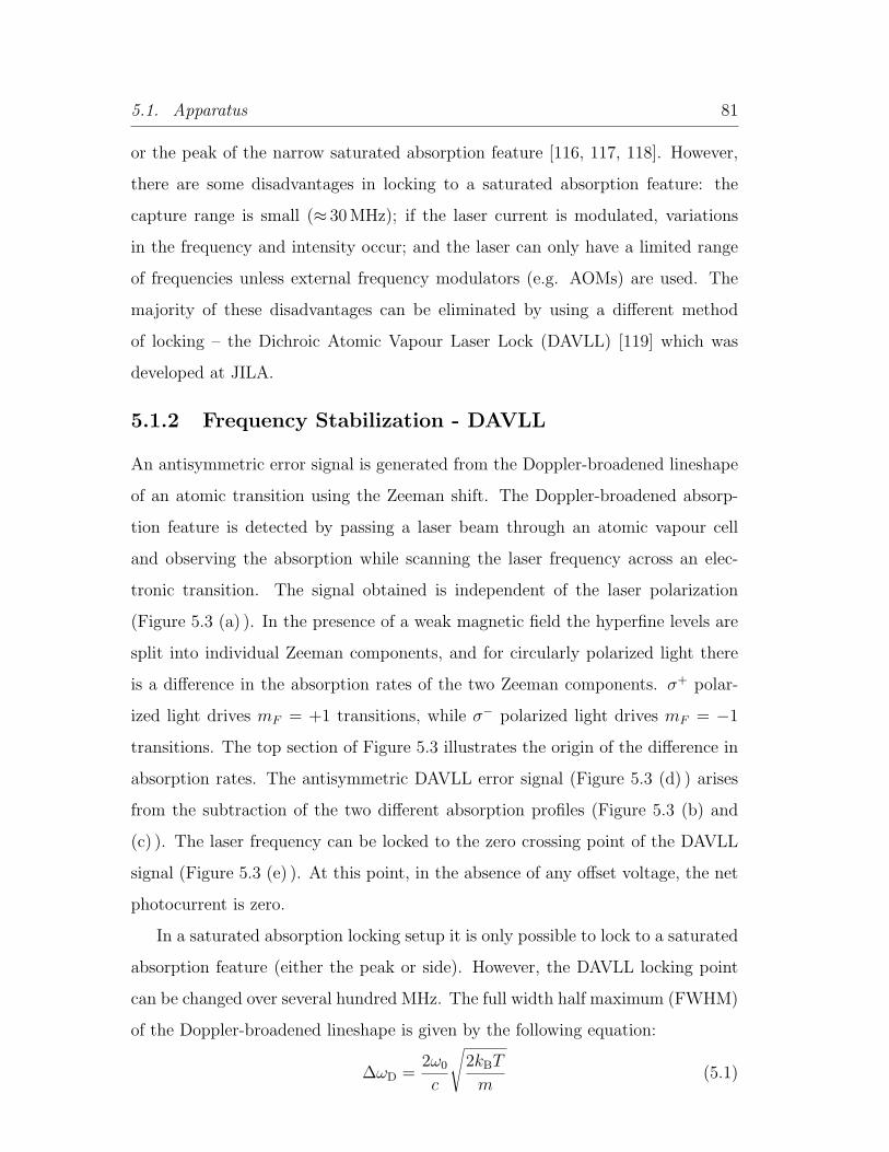
5.1. Apparatus 81
or the peak of the narrow saturated absorption feature [116, 117, 118]. However,
there are some disadvantages in locking to a saturated absorption feature: the
capture range is small (≈ 30MHz); if the laser current is modulated, variations
in the frequency and intensity occur; and the laser can only have a limited range
of frequencies unless external frequency modulators (e.g. AOMs) are used. The
majority of these disadvantages can be eliminated by using a different method
of locking – the Dichroic Atomic Vapour Laser Lock (DAVLL) [119] which was
developed at JILA.
5.1.2 Frequency Stabilization - DAVLL
An antisymmetric error signal is generated from the Doppler-broadened lineshape
of an atomic transition using the Zeeman shift. The Doppler-broadened absorp-
tion feature is detected by passing a laser beam through an atomic vapour cell
and observing the absorption while scanning the laser frequency across an elec-
tronic transition. The signal obtained is independent of the laser polarization
(Figure 5.3 (a) ). In the presence of a weak magnetic field the hyperfine levels are
split into individual Zeeman components, and for circularly polarized light there
is a difference in the absorption rates of the two Zeeman components. σ+ polar-
ized light drives mF = +1 transitions, while σ− polarized light drives mF = −1
transitions. The top section of Figure 5.3 illustrates the origin of the difference in
absorption rates. The antisymmetric DAVLL error signal (Figure 5.3 (d) ) arises
from the subtraction of the two different absorption profiles (Figure 5.3 (b) and
(c) ). The laser frequency can be locked to the zero crossing point of the DAVLL
signal (Figure 5.3 (e) ). At this point, in the absence of any offset voltage, the net
photocurrent is zero.
In a saturated absorption locking setup it is only possible to lock to a saturated
absorption feature (either the peak or side). However, the DAVLL locking point
can be changed over several hundred MHz. The full width half maximum (FWHM)
of the Doppler-broadened lineshape is given by the following equation:
∆ωD =2ω0
c
√2kBT
m(5.1)

5.1. Apparatus 82
Frequency (MHz)
-1000 -500 0 500 1000
Diff
eren
tial A
bsor
ptio
nA
bsor
ptio
n
(a)
(b)(c)
(e)
(d)
σ+ σ -
0
+1
-1
B
σ+ and σ -
E
(a)(b)(c)
0
Figure 5.3: Origin of the DAVLL signal shape: (a) the signal obtained in the absence ofa magnetic field, (b) and (c) the signal obtained in the presence of a magnetic field withσ− and σ+ polarized light respectively, (d) is the DAVLL signal obtained by subtractionof the two absorption profiles (b) and (c), (e) is the point at which the laser frequencyis locked. (Figure modified from Reference [119].)

5.1. Apparatus 83
where ω0 is the resonant frequency, T is the temperature of the atoms in the vapour
cell, and m is the mass of a caesium atom.
For caesium at room temperature (300K) the Doppler width is ≈ 450MHz.
This gives a broad locking signal which in turn makes the lock more robust. The
locking point can be changed by two methods: electronically by summing in an
external voltage to the bare DAVLL signal, or optically by rotating the quarter-
wave plate (Figure 5.4). The latter method is preferable as then the lock point
is always when the net photocurrent is zero. This means the laser frequency lock
maintains its insensitivity to laser intensity fluctuations.
Experimental Setup
The magnetic field required is produced by positioning rings of permanently mag-
netic material concentrically around the glass cell containing the atomic vapour.
The rings are separated with non-magnetic material and changing the spacing is
used to adjust the magnitude of the magnetic field to the required value. The shape
of the DAVLL signal is affected by the magnitude of the magnetic field. The larger
the magnetic field the greater the separation between the two Zeeman-shifted ab-
sorption peaks (Figure 5.3 (b) and (c) ) and the larger the capture range. The
quality of the lock however, depends on the magnitude of the slope of the DAVLL
signal at the locking point. A DAVLL signal with a steep slope makes the laser
frequency lock less sensitive to noise that mimics laser frequency changes. Another
factor relating to the magnetic field is that the Zeeman-shifted absorption peaks
broaden with increasing magnetic field. Selecting the magnitude of the magnetic
field is therefore a compromise between the size of the capture range, broadening
of the Zeeman-shifted absorption profile peaks and the magnitude of the DAVLL
signal slope. Corwin et al. [119] determined that the optimum magnetic field
value is 100 G for 85Rb/87Rb. For Cs the optimum value was found to be approx-
imately 180 G. Changes in the magnetic field of up to a factor of two should not
significantly alter the lock performance as the shape of the DAVLL signal does not
depend strongly on the magnitude of the magnetic field.
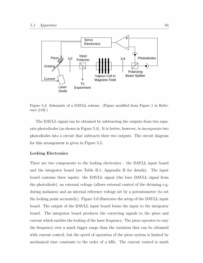
5.1. Apparatus 84
+
-
ServoElectronics
λ/4Piezo
Laser Diode
Input Polarizer
Vapour Cell in Magnetic Field
Polarizing Beam Splitter
Photodiodes
To Experiment
Current
Grating
λ/2
Figure 5.4: Schematic of a DAVLL scheme. (Figure modified from Figure 1 in Refer-ence [119].)
The DAVLL signal can be obtained by subtracting the outputs from two sepa-
rate photodiodes (as shown in Figure 5.4). It is better, however, to incorporate two
photodiodes into a circuit that subtracts their two outputs. The circuit diagram
for this arrangement is given in Figure 5.5.
Locking Electronics
There are two components to the locking electronics – the DAVLL input board
and the integrator board (see Table B.1, Appendix B for details). The input
board contains three inputs: the DAVLL signal (the bare DAVLL signal from
the photodiode), an external voltage (allows external control of the detuning e.g.
during molasses) and an internal reference voltage set by a potentiometer (to set
the locking point accurately). Figure 5.6 illustrates the setup of the DAVLL input
board. The output of the DAVLL input board forms the input to the integrator
board. The integrator board produces the correcting signals to the piezo and
current which enables the locking of the laser frequency. The piezo operates to vary
the frequency over a much bigger range than the variation that can be obtained
with current control, but the speed of operation of the piezo system is limited by
mechanical time constants to the order of a kHz. The current control is much

5.1. Apparatus 85
10kΩ
10kΩ
22kΩ
22kΩ
100Ω
0.5MΩ
TL081
+V
-V
+
-Vout
Figure 5.5: Diagram of the double photodiode (BPX65) circuit. The basic circuit is acurrent-to-voltage converter. The difference in the two photocurrents is converted intoa voltage by the operational amplifier (TL081).
faster and therefore it can be used to reduce noise over a wider band than could
be attained with only a piezo. The piezo operates to take out the effects of slower
drifts and the effects of vibration, whereas the current lock is used to compensate
for higher frequency noise. The changeover frequency between the current and
piezo lock depends on the response time of the piezo.
There are many advantages in using the DAVLL system, rather than saturated
absorption, to lock the laser frequency:
• It is compact and simple to set up – it requires very few optics and simpler
electronics.
• It requires less laser power to lock.
• It has a large recapture range therefore the laser frequency stays locked for
much longer periods of time.
• There is no need for modulation of the laser current.

5.1. Apparatus 86
Photodiode Signal
Internal Voltage
External Voltage
+
-
Integrator Board
Polarity Switch
-
++10 V
-10 V
. .
.
Figure 5.6: A schematic of the DAVLL input board illustrating the three inputs and theoutput, and the general flow of the circuit.
• Large frequency changes are possible by applying an external voltage (as
explained previously). This is a significant advantage, not only in cost, but
the use of an AOM in a double-pass configuration leads to at least a 50%
reduction in laser power.1
One disadvantage of the DAVLL scheme of locking the laser frequency is that
it is impossible (without extra apparatus) to observe variations in the detuning
frequency. One method of overcoming this disadvantage is to use a saturated
absorption setup for comparison (see Figure 5.2 for an example of a laser setup
incorporating both DAVLL and saturated absorption setups). The laser frequency
is locked using the DAVLL signal and the point at which it is locked is set to be
on the peak of a saturated absorption feature. The laser frequency is therefore
locked using the DAVLL scheme, but with the ability to maintain close observa-
tion of the laser detuning. This is important as laser detuning has a large effect
on experimental reproducibility. The DAVLL signal is also calibrated using the
saturated absorption signal. By noting the position at which each Lamb dip in
the saturated absorption signal occurs as a function of DAVLL detuning voltage,
a curve is generated which gives the relationship between the DAVLL detuning
voltage and the absolute detuning in MHz.2
1For large frequency changes an AOM must be used in a double-pass configuration.2When the DAVLL signal is linear across all of the saturated absorption peaks the detuning
(in MHz) is directly proportional to the detuning voltage.

5.1. Apparatus 87
Experimental Setup
The DAVLL scheme has been used to lock the frequencies of all three external cav-
ity diode lasers (ECDL) on the experiment for the last three years. One important
point that should be noted is that the quality of the laser frequency lock seemed
to depend largely on the quality of the laser mode.
During the experiment’s day-to-day running the lasers rarely jumped out of
lock. When they did, it could normally be attributed to the laser jumping to a
different mode of the laser chip. Normal mechanical noise (e.g. tapping the optic
table) and high frequency noise (e.g. pulsed copper vapour laser operation in the
room directly above the laboratory) did not seem to have an effect on the lock.
Due to the effect a slight change in detuning can have on experimental repro-
ducibility, the detuning of each laser was carefully monitored. The detuning of
the MOT laser could drift significantly over the course of the day. This was at-
tributed to the poor mode structure of the laser. The probe and the repumping
laser detunings were checked approximately every 20 minutes.
Probe Laser
As mentioned previously the probe laser light is used not only for probing but also
for optical pumping. The laser must therefore be jumped from the F = 4 → F ′
transition to the F = 3 → F ′ transition. Initially the laser frequency is locked
to the F = 4 → F ′ = 5 : F = 4 → F ′ = 4 cross-over transition.3 The laser is
unlocked by applying a low TTL signal to the gate input of the integrator board.
The current and the PZT values are changed to the appropriate values for the
F = 3 → F ′ transition by applying voltages to the current and PZT feed forward
inputs on the integrator board. The detuning of the laser frequency is also changed
by applying a voltage to the external voltage input on the DAVLL input board.
The laser frequency is then locked to the new frequency by applying a high TTL
signal to the gate input of the integrator board. This process is carried out before
3The AOM frequency is set to be 125.7 MHz, bringing the frequency of the laser radiationincident on the atoms to the frequency of the cycling transition.

5.1. Apparatus 88
the optical pumping and then the reverse process (re-locking the laser frequency
to the cooling transition) is carried out after loading the magnetic trap.
5.1.3 The Optical Table
The main optical table was divided into two sections: the laser section and the
experimental section.
The laser section consisted of most of the equipment required to produce the
frequencies required for cooling, trapping, and probing of the atoms. Figure 5.7
is a schematic of the laser section. The repumping laser and its optical setup
(Figure 5.2) was situated on another smaller optical table. The light from this
table was coupled down an optical fibre and the fibre end was situated on the
main optical table to allow for coupling of the repumping and MOT light on a
beam-splitter cube.
The probe laser is situated on the upper half of the optical table (Figure 5.7),
and all the optics required for locking of the laser frequency is illustrated. An extra
saturated absorption optical setup after the AOM permits the observation of the
detuning of the laser light after the AOM and prior to coupling the light down the
fibre.
The light from the MOPA is divided into two using a half-wave plate. This
half-wave plate is used to set the powers on the pyramid and the experimental
MOT. Each beam then passes through an AOM. Both AOMs are required to
permit separate modification of the pyramidal MOT and experimental MOT light
detuning as both beams are derived from the same laser (Master). Each beam is
then coupled with the repumping light on a beam-splitter cube, and then coupled
down an optical fibre. The optical fibres are then passed through a small hole
into the experimental section of the optical table. The experimental section was
enclosed in a light-tight box to prevent scattered light from reaching the atoms.
The experimental setup is illustrated in Figure 5.8.

5.1. Apparatus 89
Flipper Mirror
Probe
AOMA
OM
AOM
DAVLL cell
λ/4
Glass plate
f=25cm
Photodiode
λ/2
Master
λ/2
λ/2
f=25cm
Probe and Optical
Pumping
MOPA
Beam Splitter
λ/2
λ/2λ/4
DAVLL cell
Photodiode
Photodiode
λ/2
λ/2
λ/2
λ/2
λ/2
λ/2
λ/2
Isolator
λ/2
λ/2
f=10cm
f=10cm
f=25cm f=25cm
f=25cm
f=25cm
ShutterShutter
Isolator
f=10cmf=10cm
f=10cmf=10cm
From Repumper
Setup
Shutter
Shutter
Isolator
Caesium Vapour Cell
Caesium Vapour Cell
CaesiumVapour
Cell
To Pyramidal
MOT
To Experimental
MOT
Cylindrical Lens
Isolator
Figure 5.7: A schematic of the laser table.
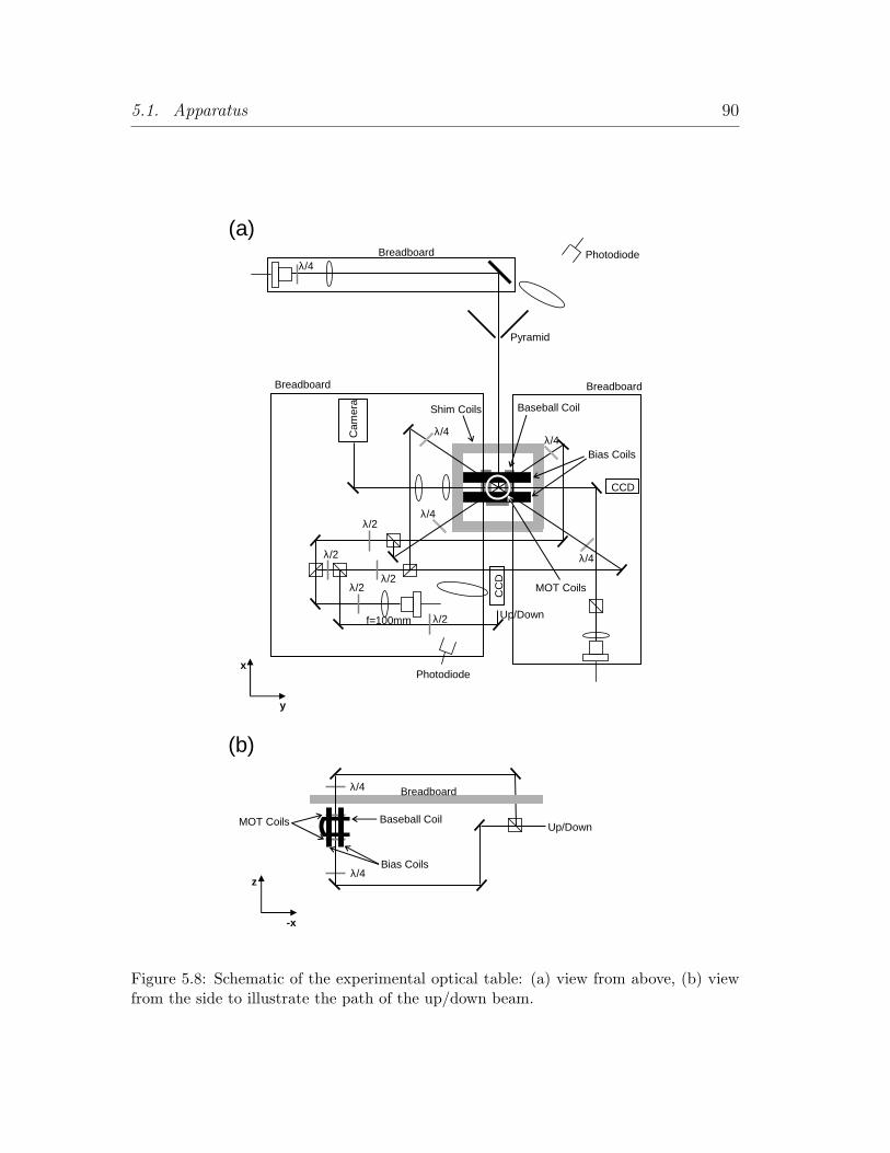
5.1. Apparatus 90
Cam
era
CC
DCCD
λ/2
Photodiode
λ/4
Pyramid
Up/Down
Photodiode
Up/Down
λ/4
λ/4
Breadboard
Breadboard
Breadboard
Breadboard
λ/4λ/4
λ/4
λ/4
λ/2
λ/2λ/2
λ/2
(a)
(b)
f=100mm
Bias Coils
Baseball CoilShim Coils
x
y
z
-x
MOT Coils
MOT Coils
Bias Coils
Baseball Coil
Figure 5.8: Schematic of the experimental optical table: (a) view from above, (b) viewfrom the side to illustrate the path of the up/down beam.

5.1. Apparatus 91
Ion pump40 l/s
Ion pump55 l/s
valve
Getter pump
Distance betw
een MO
Ts
300 mm
Pyramidal MOT
Glass cell
Figure 5.9: An illustration of the vacuum system.
5.1.4 Vacuum System
The vacuum system shown in Figure 5.9 can be discussed in two parts.
The first section of the vacuum system contains the pyramidal MOT. It has a
pressure of approximately 10−9 mbar maintained by a 40 l/s ion pump (Varian Va-
cIon Plus 40). The caesium source is several dispensers (SAES Getters) connected
in series located just above the pyramid mirrors. A current is passed through the
dispensers, generating heat and the resulting chemical reaction releases caesium
atoms. The dispenser is continually operated at 3.2A to provide ample Cs pressure
in the pyramidal region.
Differential pumping is achieved by a hole (5mm diameter, 17mm long) in the
back port of the first chamber. The distance between the pyramidal MOT and the
experimental MOT is 30 cm. This distance is short in order to reduce atom loss due
to divergence of the atomic beam from the pyramidal MOT to the experimental
MOT.

5.1. Apparatus 92
The second section of the vacuum system contains a rectangular quartz cell
of dimensions 28 × 28 × 80 mm3 (2mm wall thickness). Pressure in this region is
maintained by a 55 l/s ion pump (Varian VacIon Plus 55) and a non-evaporable
getter (NEG) pump (SAES CapaciTorr-CF35, Cartridge C-400-DSK-St172). The
NEG pump should preserve a very low pressure in the experimental cell for long
term operation.
5.1.5 Pyramidal MOT
The purpose of the pyramidal MOT [72] is to collect atoms from a vapour of
caesium. The atoms are transferred continuously through the differential pumping
hole into an ultra-high vacuum region, where the final experiments are performed.
Our pyramid ( Figure 5.10 ) is larger than the one described in Reference [74]. This
is an improvement as an increase in the size of the pyramidal mirrors increases the
volume of the collection region, which results in a higher flux atomic beam.
Experimental Setup
The pyramidal MOT experimental apparatus can be divided into two distinct
parts: the optical arrangement and the generation of the magnetic fields required.
The optical setup is straightforward (see Figure 5.11). The large mirror (di-
ameter = 100mm) and the pyramidal mirrors (base length = 60 mm) are coated
by C. Goodwin in the Oxford physics department. The mirror and pyramid optics
are coated to achieve the same reflectivity for s- and p-polarization.4 The beam
size required is approximately 60mm therefore a single lens (f=250mm) after the
bare fibre end provides both the magnification and collimation. The initial reason
for using a fibre was because of the poor beam quality of the MOPA. However,
an added advantage was soon realised. When the pyramid was first set up, the
pyramidal light was derived from a single laser (with no fibre). Because of the
long path length from the laser to the pyramidal mirror, any slight changes in the
angle of the grating of the ECDL caused a large deviation in the incident position
4Non-equal reflectivity between s- and p-polarization causes a phase shift between the twopolarizations and therefore the light is no longer circularly polarized.

5.1. Apparatus 93
Shim Coil
Pyramidal Mirrors
Caesium Dispensers
Differential Pumping Hole
Figure 5.10: A photo of the pyramid.

5.1. Apparatus 94
λ/4f=250mm
f=100mm
100mm
100mm
Figure 5.11: A diagram of the optical setup of the pyramidal MOT.
of the beam on the pyramidal mirrors. This caused a drastic change in the loading
performance of the pyramid and meant that it was necessary to adjust the large
pyramid mirror every day. Once the MOPA was set up and the fibre implemented,
the beam angle was carefully set up and the shim coil settings optimized. Over
the course of the last two years the pyramidal experimental parameters (e.g. beam
angle, quad-coil current, shim coil settings) have not been changed. Every morning
the only optimizations that were carried out on the pyramid were: optimizing the
transmission of the pyramid light through the fibre, and a slight adjustment of
the quarter-wave plate to compensate for drifts in the output polarization of the
optical fibre. The optimum position of the wave plate was decided by optimizing
the load of atoms into the experimental MOT or by looking at the quality of the
pyramidal or experimental MOT using an infrared camera.
Two sets of coils are required for generation of the magnetic fields required: a
pair of anti-Helmholtz coils (pyramid quad-coils), and three shim coils (pyramid
shim coils) positioned in orthogonal directions.
The anti-Helmholtz coils provide the field gradient required for confinement
of the atoms. They are made out of 15 turns of 3mm outer diameter 22 swg
(corresponding to an inner diameter of approximately 1.5mm) annealed copper
tubing. Water is passed through the copper tubing to provide cooling. The radius

5.1. Apparatus 95
of the coils is 56mm and their separation is 50mm. To load the atoms 18A is run
through the coils producing a field gradient of 9.22G cm−1 (Equation 2.8). The
total resistance of the pyramid quad-coils (in series) and the connecting cables is
approximately 0.08Ω.
The shim coils are circular coils, inner diameter of approximately 150mm,
wound out of 1 mm (100 turns) enamelled copper wire. There are two purposes for
the 3 shim coils: firstly any ambient magnetic fields (e.g. earth’s magnetic field)
need to be nulled out, and secondly they are required to move the centre of the
magnetic field produced by the quad coils for diagnostic purposes. In order to
determine the number of atoms in the pyramid accurately, it is necessary to move
the centre of the MOT to a position where the fluorescence can be measured. Nor-
mally the centre of the MOT is over the pyramid hole and therefore no fluorescence
is observed. The voltage level circuit (Section 5.2.2) provides the voltages for the
two settings required – one for loading the experimental MOT and the reference
setting for determining the atom number in the pyramid.
5.1.6 2nd MOT – Experimental MOT
For this experiment the 2nd MOT is a conventional six-beam MOT [58].
The MOT quad coils are circular coils of diameter 50mm separated by a dis-
tance of 70 mm. Each coil is made out of 80 turns of 1 mm enamelled copper
wire. The wire is wound onto a water-cooled former as in the absence of water-
cooling the temperature of the coils reaches 100 oC within 5 minutes. The coils
are positioned as close as possible to the trapping region as the amount of current
required to produce a given gradient is proportional to the separation of the coils
to the fourth power (I ∝ s4). Figure 5.12 illustrates the position of the MOT quad
coils. To load the experimental MOT 2.26A is run through the quad coils. This
generates a field gradient of 10.2G cm−1 (Equation 2.8). The current through the
coils is controlled by a FET and the gate voltage for the FET is provided by the
multiplexer circuit (see Section 5.2.2).
Shim coils are required to null out any ambient fields, which is especially im-

5.1. Apparatus 96
Shim Coils
Baseball Coil
Bias Coils
MOT Coils
Glass Cell
Figure 5.12: A photo of the experimental MOT. The baseball coil surrounds the glasscell. The MOT coils are positioned between the baseball coil and the bias coils.
5.1. Apparatus 97
portant in the optical molasses stage of the experiment, and to move the centre of
the MOT for loading into the magnetic trap. The shim coils are six rectangular
coils mounted in a cuboid arrangement. The lengths of the side are approximately
164mm and the separation between the coils is approximately 90mm (taking into
account the thickness of the windings). Each coil consists of 50 turns of 1mm
enamelled copper wire. The y-z direction shim coil is also used to produce the
quantization field for probing and optical pumping. The magnitude of the quanti-
zation field is approximately 3 G.
The optics for the experimental MOT is illustrated in Figure 5.8. It is possible
to generate the three pairs of orthogonal counter-propagating beams required by
retro-reflecting three individual beams. However, because of the optical absorption
of the cloud, this method introduces a power imbalance between each counter-
propagating beam. This problem is avoided by using six separate beams.
5.1.7 Magnetic Trap
The magnetic trap used in the experiment is a baseball trap (Section 2.4.5, Chap-
ter 2). This type of trap was chosen because it is possible to attain high magnetic
fields and weak trapping potentials simultaneously. The baseball coil is capable of
generating axial and radial confinement. However, a pair of Helmholtz coils (called
bias coils) were added in order to permit modification of the trapping geometry.
The bias coils can either be set up to add to or oppose the axial magnetic field
generated by the baseball coil. When they are set up to oppose they produce
tight radial confinement at low fields, whereas for addition they provide the ability
of operating at high magnetic fields (over 500G). Figure 5.13 is a photo of the
baseball and bias coils.
The baseball coil is constructed using 1/8” outside diameter 22 swg (corre-
sponding to an inner diameter of approximately 1.5 mm) annealed copper refriger-
ation tubing. The bias coils are constructed out of 3/16” 20 swg (corresponding to
an inner diameter of approximately 3mm) annealed copper refrigeration tubing.
The baseball and bias coils both consist of 9 turns. Before winding the coils, the

5.1. Apparatus 98
Figure 5.13: A photo of the baseball and bias coils.
copper tubing is encased in heatshrink to insulate the turns. During the winding,
all the voids between the layers of copper tubing are filled with epoxy to improve
mechanical stability.
The hollow tubing allows for water cooling of the coils, which is necessary as
high currents (up to 500A) generate a significant amount of heat. Thermistors are
glued to the baseball and bias coils and are connected to the temperature interlock
facility of the high current power supply. If the temperature exceeds the preset
temperature (set by a potentiometer), the circuit trips, turning off the current.
Control Electronics
The magnetic trap current is controlled by two pairs of electronic circuits – a
‘Reference Voltage Board’ and ‘Main Feedback Board’ (see Figure 5.14). The
‘Reference Voltage Board’ controls the trap turn on/off (and fast input control
etc) and generates the input voltage for the ‘Main Feedback Board’. The ‘Main
Feedback Board’ provides the gate voltage for the FET’s and the integrator part
of the circuit regulates the current through the baseball and bias coils.
The ‘Trap on/off TTL’5 is controlled by a TTL signal. When the TTL signal
5In the following section, all signal names in inverted commas refer to the corresponding

5.1. Apparatus 99
EW1285 –
Reference Voltage Board
EW1282 –
250A Coil Driver
Main Feedback Board
Labview Input Voltage
Trap on/off TTL
Ext/Int Control TTL
Fast Input Enable TTL
Fast Input
Internal Voltage Potentiometer
Output Voltage
Control Voltage
Gate Voltage
TC Switch 1 TTL
TC Switch 2 TTL
Current Monitor
Sensor Input
Sensor Output
Hall Sensor
500A @ 8V
HP Power Supply
Figure 5.14: A schematic illustrating the setup of the magnetic trap current controlelectronics. (To control the current in both the bias and baseball coils two pairs of theabove boards are required.)

5.1. Apparatus 100
is set to high, the trap turns on to a level set by the analogue ‘Labview Input
Voltage’. For a rapid turn on the trap is turned on with the servo capacitors
switched out of the circuit. The capacitors are then switched back into the circuit
to improve DC stability.
For fast current control the fast input facility can be used. The ‘Fast Input
Enable TTL’ requires a TTL signal in order to switch an extra reference voltage
into the circuit. The extra reference voltage is an analogue voltage applied to the
‘Fast Input’, and is then summed into the circuit. This facility is required as the
analogue input from Labview is filtered (the ‘fast input’ is summed into the circuit
after the filter) and therefore fast current changes cannot be implemented.
The magnetic field stability depends partly on the stability of the analogue
outputs of the computer board. The ‘Labview Input Voltage’ can be switched
down by a factor of a 100 using the ‘Ext/Int Control TTL’. Simultaneously the
stable reference source can be switched in. This stable reference source is produced
on the ‘Reference Voltage Board’ by a series of resistors and a potentiometer for
small adjustments. During the life of the experiment this feature has been used
sparingly. There has not been a reason to believe that any possible noise from the
computer board was having a detrimental effect on the experimental results.
The ‘Main Feedback Board’ generates the gate voltage for the FETs. The
FETs that are used on the experiment are capable of running 200A each. There
are 10 FETs in total – 5 for the bias coils and 5 for the baseball coil. The current
source is a Agilent power supply (Agilent 6681A) capable of running 500A at 8V.
Welding cable is used to carry the current from the power supply to the coils.
For current stabilization the welding cable is passed through two closed loop
current sensors (one for each coil). The ‘Main Feedback Board’ generates and
controls the current in the Hall sensor. It produces a magnetic field that cancels
the magnetic field due to the current flowing through the welding cable. Any
changes in the current are observed by converting the current flowing through the
Hall sensor into a voltage. The voltage is measured using a 6 d.p. precision DVM
input/output in Figure 5.14
5.1. Apparatus 101
(Agilent 34401A – 6 1/2 Digit Multimeter). Therefore field fluctuations of the
order of a few mG can be observed. This voltage is also used as an error signal to
regulate the current through the coils.
For normal running of the experiment the current in the baseball coil, ≈ 230
Amps, is turned on in under 400 µs to give a magnetic field value of ≈ 139 Gauss
at the centre of the trapping potential. This results in trap frequencies of 12 Hz
radially and 5Hz axially.
Classical Motion of Atoms in a Magnetic Trap
In a purely parabolic potential, with no collisions between atoms, atoms undergo
simple harmonic motion in each orthogonal direction. However, it is experimentally
impossible to construct a magnetic trap where the potential is purely parabolic.
There exist cross-terms in the potential equation which break the separability of
the three spatial dimensions, and in turn cause the orbits of the atoms to slowly
precess. This leads to a mixing of energy between spatial directions.
There are two main problems which can result upon loading of the magnetic
trap: sloshing and breathing.
Sloshing is the motion of the centre of mass of the cloud that occurs when the
atoms are not loaded into the centre of the trapping potential, or if the cloud is
loaded into the magnetic trap with some velocity. Atoms at different points in the
cloud will therefore have different amplitudes of oscillations, and in a harmonic
trap, the cloud will undergo simple harmonic motion about the minimum of the
magnetic trapping potential. Anharmonic terms in the trapping potential will
cause the cloud to spread out over the region in which it was sloshing. As the
width of the cloud is greater, it appears that the temperature of the cloud has
increased. The magnitude of the sloshing can be reduced by better matching of the
MOT and magnetic trap centres by use of the shim coils during the CMOT stage.
Figure 5.15 illustrates the sloshing in the axial and radial directions. Sloshing can
be used to determine the trapping frequencies, as described in Section 5.4.6.
After loading the magnetic trap, if the shape of the MOT does not match the

5.1. Apparatus 102
0 200 400 600 800 1000 1200 1400260
265
270
275
280
285
290
Axia
l Cen
tre (p
ixel
)
Time (ms)
0 200 400 600 800 1000 1200 140085
90
95
100
105
110
115
120
125
(b)
Rad
ial C
entre
(pix
el)
Time (ms)
(a)
Figure 5.15: Observation of the sloshing in the axial and radial directions. Each pointrepresents a single measurement (both radial and axial position) of the centre of massof the cloud, while it sloshes in the trap.

5.1. Apparatus 103
0 200 400 600 800 1000 120052
54
56
58
60
62
64
66
68
70
72
74
Axi
al S
igm
a (p
ixel
)
Time (ms)
Figure 5.16: Observation of the axial breathing mode in the magnetic trap. The fre-quency of the breathing motion is approximately 10.6Hz, which corresponds to an axialtrap frequency of 5.3 Hz.
shape of the MT contours then the initial potential and kinetic energy will not be
in equilibrium. This leads to an excitation of the breathing mode. The width of the
cloud will oscillate, leading again to an increase in the temperature of the cloud.
The breathing mode frequency is twice the trap frequency (due to the symmetry of
the trapping potential). To reduce the likelihood of exciting the breathing modes,
the parameters of the molasses stage are adjusted in order to match the shape
of the cloud to the magnetic potentials. Figure 5.16 is a graph illustrating the
breathing mode of the atom cloud in the magnetic trap.
The six MOT laser beams on the experiment are not aligned perfectly orthog-
onal (due to optical access constraints). The cloud is therefore not spherical and is
slightly elongated in the x - direction. This coincides with the shape of the mag-
netic field contours in the same direction. (Figure 2.11 shows that the magnetic
field contours are elongated in the x - direction.)

5.2. Control 104
5.1.8 Evaporation
The radio-frequencies required for evaporation were generated by a frequency gen-
erator (Agilent E4400B). The signal is amplified by a Minicircuits amplifier (ZHL-
5W-1 for 40 dB gain) and is transmitted to the atoms via a two-turn coil. A
10Ω resistor was placed in series with the coil to impedance match the load to
the source. This should reduce amplitude changes over the range of frequencies
used. The evaporation ramps were calculated in Labview and then transferred
continuously to the frequency generator via GPIB interface.
5.2 Control
When setting up an experiment a choice has to be made between an analogue
or a digital basis for experimental synchronization. The difference between both
approaches is: in the analogue setup the computer generates the analogue voltages
and therefore external electronics (e.g. Schmitt triggers) are required to synchro-
nize the equipment; whereas in the digital setup the computer generates the TTL
signals required to synchronize the equipment, and external electronics are required
to produce the analogue voltages.
The advantages of the digital philosophy is that TTL signals have a high fidelity
and therefore there is no degradation of the signal along long BNC cables. It
is straightforward to implement as there is no timing issues with TTL signals.
Experiments based on the digital philosophy are very easy to run on a day-to-day
basis as unknown experimental problems are simpler to solve when each section of
the experiment can be disassociated from other sections.
5.2.1 Experimental Synchronization
This experiment was built using the digital philosophy. The experiment was syn-
chronized using a Labview control program connected to the experiment with two
data acquisition boards (a digital and an analogue board) and a GPIB board (see
Appendix B). Two analogue outputs are used: ‘Labview Input Voltage’ for the

5.2. Control 105
bias and baseball coil (Figure 5.14).
Labview
One of the advantages of using the Labview program to control the experiment is
its user-friendly interface. The control program was written [120] by first setting
up the correct experimental timing structure as in Figure 5.17. The timing delays
(e.g. shutter delays, quad current turn on time etc) are then entered into a table
which is incorporated into the program with the use of equation boxes. This means
that any subsequent modifications in the timings does not involve a restructuring
of the program.
5.2.2 Analogue Voltages
The digitization of the experiment does mean that other methods of generating
the analogue voltages are required. A multiplexer circuit and a voltage switching
circuit (see Table B.1, Appendix B) are used to generate analogue voltages. They
both work on the same principle – applying a TTL signal switches between two
analogue voltages (range -10 to 10V). The voltages required are set using panel-
mounted potentiometers. The multiplexer circuit uses two input TTL signals to
switch between four analogue voltages. This circuit is used for the experimental
MOT quad and shim coil voltages and the MOT laser detuning settings – each of
which require 4 different experimental settings (i.e. for loading the MOT, CMOT,
molasses and optical pumping). The voltage switching circuit (one TTL signal)
is used for the pyramid quad and shim coils and the probe detuning, current and
PZT feed forward values.

5.2. Control 106
A0
Tra
p o
n/o
ff
A1
Ext
/Int
Co
ntr
ol
A2
BB
Cap
s
A3
Bia
s C
aps
A4
Fas
t In
pu
t E
nab
le
B0
Pyr
amid
Sh
utt
er
B1
MO
T S
hu
tter
B2
Pro
be
Sh
utt
er
B3
Rep
um
p S
hu
tter
B4
Pro
be
Sw
itch
B5
Pro
be
Att
en.
C0
MO
T D
et 1
C1
MO
T D
et 2
C2
Pro
be
Det
.
C3
Pro
be
Ffw
d
C4
Pro
be
Lo
ck
C5
HF
P D
et 1
C6
HF
P D
et 2
D0
Pyr
amid
Sh
ims
D1
MO
T S
him
1
D2
MO
T S
him
2
D3
Pyr
amid
Co
il
D4
MO
T C
oil
1
D5
MO
T C
oil
2
Lo
adin
g M
OT
MO
TC
MO
TM
ola
sses
2nd
Imag
e3r
d Im
age
OP
Mag
net
ic T
rap
Exp
erim
ents
1st
Imag
e
Figure 5.17: Idealized timing diagram. A grey line / grey box indicate a low / highlevel TTL signal. The logic state of the experiment at a particular time can be clearlyobserved by reading down the columns e.g. for the CMOT the digital signals are 0 0 00 0 1 0 1 etc.

5.3. Diagnostics 107
F = 100mm
∅∅∅∅ = 60mm
NA = 0.3
F = 14mm
∅∅∅∅ = 12mm
NA = 0.43
56mm
84mm
19mm150mm300mm
Light-tight tube
Photodiode
3.6x3.6mmObject
Figure 5.18: Fluorescence measurement setup for the experimental MOT. The rele-vant equations to convert the photodiode photocurrent into number are given in Refer-ence [68].
5.3 Diagnostics
Most of the information that has been obtained on BECs and thermal clouds have
been obtained by optical diagnostics. Two of the most important diagnostic meth-
ods are in-situ and time-of-flight (TOF) imaging. These correspond to imaging
the cloud in its trapped state and then the subsequent ballistic expansion from the
trapped state respectively.
5.3.1 Recapture
For diagnostic purposes it is important to be able to determine the number of
atoms in the experimental MOT and also in the magnetic trap. The simplest
diagnostic method for determining atom number is measuring the fluorescence
emitted by the atoms. A large collection lens is placed as close as possible to the
atoms and a photodiode is then placed at the focal point of the lens. Figure 5.18
illustrates our fluorescence setup, which includes two lenses and a light-tight tube
to improve signal-to-noise ratio. The fluorescence measured by the photodiode is
then converted into number with the equations given in Section C.3, Appendix C.
These equations derive from Reference [68].

5.3. Diagnostics 108
5.3.2 Absorption Imaging
Absorption imaging is the most commonly used method of diagnostics in atom
optics experiments, because it not only yields information on number but also the
cloud’s spatial parameters.
Optical Depth
The optical depth (OD) at a point in the cloud is proportional to the column
density at that particular point. The equation for the optical depth is:
I = I0 exp(−OD(x, z, ∆)) (5.2)
where I is the transmitted intensity and I0 is the intensity of the incident beam.
Equation 5.2 only holds for low intensities.6
Many factors affect the observed OD. Light is scattered not only from the
atoms, but from any imperfections in any of the optical elements in the imaging
system. The observed OD is therefore lower than the actual OD.
The maximum observable OD also depends on the size of the cloud. The
smaller the cloud the lower the maximum observable OD, because it easier for the
light scattered at the edge of the cloud to fill in the centre of the shadow. High
magnification imaging systems make this effect worse.
Interference fringes in the probe beam can cause problems when imaging.
Fringes can occur due to diffraction from the glass cell, waveplates, mirrors, lenses
and the CCD array window. If the fringe pattern is stable, i.e if the fringes do
not change between images, then subtracting an image of the probe beam from an
image containing the atoms will eliminate the fringes. However, if the fringes do
move then subtracting the image of the probe beam will actually worsen the effect.
As long as the spatial size of the cloud is different to the spatial frequency of the
fringes, fitting Gaussian distributions to the cloud tends to eliminate this effect.7
6For a detailed discussion on optical depth and saturation intensity see Reference [84].7For a low optical depth cloud the effect is amplified as the apparent optical depth of the
fringes will dominate the resulting profile.

5.3. Diagnostics 109
f1 f2
d
Atoms
Laser radiation
CCD Array
Figure 5.19: Schematic of the imaging setup.
Experimental Setup
The optical setup used for absorption is illustrated in Figure 5.19. The focal
length of the two lenses are chosen depending on the magnification required. The
magnification is the ratio of the two focal lengths (f2/f1).
To image the atoms, the current in the magnetic trap coils is turned off (in
less than 300µs) and the atoms are pumped into the F = 4 sublevel with a 150 µs
pulse of light resonant with the 6S1/2, F = 3 → 6P3/2, F′ = 4 transition. The cloud
is then probed by applying a 50 µs pulse of circularly polarized light resonant with
the 6S1/2, F = 4 → 6P3/2, F′ = 5 transition. An AOM is used for fast shuttering of
the probe light.8 The intensity of the probe beam is generally no greater than 10 %
of the saturating intensity, and therefore Equation 5.2 is valid. The quantization
field is the same as that required for the optical pumping. The shadow of the
atoms in the beam is then imaged onto a CCD array.
The CCD array is part of a camera manufactured by Andor. The Andor camera
on the experiment (DV437-FI, serial number: CCD-2611) is a frame-transfer cam-
era and is ideal for fast imaging applications. The CCD array consists of 512× 512
pixels and the pixel size is 13 µm2. The maximum frame readout per second is 3.2
which increases to 10.0 if 4 × 4 binning is used.
The control system for the the Andor camera is a Multi I/O Box (IO160).
This in combination with the Labview program (which controls the experiment)
8A mechanical shutter is also included on the probe beam path (see Figure 5.7) to preventany probe light from reaching the atoms when they are in the magnetic trap.

5.3. Diagnostics 110
provides the means of controlling the image acquisition. The auxiliary output of
the Multi I/O Box is set to low when the Andor software is ready for an image.
Once an image is ready to be taken Labview sends a high TTL signal to the
external trigger input of the Multi I/O Box to arm the camera. When the image
is taken a high TTL signal is sent to the fire input of the Multi I/O Box. Once the
images have been acquired Andor then sets the auxiliary output on the Multi I/O
Box to high to prevent further images being taken before the images have been
downloaded into the computer.
Normally three images are taken. The first image is taken after a controlled
TOF (I1), the second is an image of the probe beam taken as soon as possible
after the first image (I2), and the third image is of the background and scattered
light (I3). The background image is subtracted from both the first two images,
the two files are then divided and then the natural log of the resulting file is taken
(Equation 5.3):
OD = ln(
I2 − I3
I1 − I3
)(5.3)
This image is then summed in both directions and the resulting profiles are
fitted with a Gaussian function (Equation 5.4) from which values for the peak
optical depth and the widths can be extracted.
Optical depth summed in the y direction = exp−x2
2σ2(5.4)
Knowing the magnification and the magnetic field parameters, physical quanti-
ties (e.g. density, temperature) can be derived from the data using the following
equations:
Radial Temperature, Tr =mω2
rσ2r
kB
(5.5)
Number, N =2πODpkσrσz
σ0
(5.6)
Peak Density, npk = Nω2rωz
(m
2πkBT
) 32
(5.7)
where σ0 = 3λ2/2π, σz and σx are the widths of the cloud in the axial and radial
directions respectively.

5.3. Diagnostics 111
Focussing and Magnification
The imaging system needs to be focussed in order to obtain accurate values for
the cloud widths. The focussing is done by firstly creating a very small cloud. The
second lens of the imaging system (Figure 5.19) is mounted on a translation stage
capable of micron precision adjustment. A graph is plotted of the radial width of
the cloud versus the position of the second lens. The minimum in the radial width
corresponds to the focussed position of the second lens.
The magnification of the imaging system can be determined by plotting the
radial centre of the cloud versus the TOF. By fitting
s′ = s +1
2g′t2
to the data, where s is the actual displacement, g′ is the apparent acceleration
due to gravity and t is the value of the TOF, a value for the apparent acceleration
due to gravity (g′) is obtained. The value obtained from the fit depends on the
size of the pixel and the magnification of the imaging system. This value is then
compared to the actual value of the acceleration due to gravity (g) to determine
the magnification:
M =g′∆x
g
where M is the magnification, ∆x is the pixel size in µm, and g is the acceleration
due to gravity. For the data in Figure 5.20 the magnification is 1.008(7).
Lensing Effects
If the probe beam is detuned from resonance, the refractive index of the cloud is
no longer 1 and because of the variations in the density across the cloud, the cloud
acts like a lens. If the imaging system is focussed, no change in the shape of the
cloud is observed when the probe beam is detuned. However, if the cloud is out of
focus then the cloud shape becomes very distorted. This lensing effect can be used
as another method of focussing the cloud i.e. the appearance of the cloud should
not change with the detuning (red or blue) of the probe light when the imaging
system is in focus.

5.3. Diagnostics 112
0 2 4 6 8 10 12 14 16 18 20 2260
80
100
120
140
160
180
200
220
240
Rad
ial C
entre
Time of Flight (ms)
Figure 5.20: Determining the magnification of the imaging system. The accelerationdue to gravity given by the fit is 0.76 m s−2. This value must be compared to the actualacceleration due to gravity in order to determine the magnification.
5.3.3 Comparison of Recapture and Imaging
Most experimental results are obtained by imaging the cloud. However, recapture
measurements can sometimes be the only method of reliably obtaining the atom
number.
Imaging large atom densities is difficult as lensing effects can distort the number
measurement. MOT recapture measurements do not suffer from this. Another
advantage of MOT recapture measurements is that the fluorescence can be read
straight off an oscilloscope connected directly to the photodiode (a photodiode
circuit contains a current-to-voltage follower). To obtain the atom number there
is therefore no need for a probe beam and expensive CCD camera or any data
processing. The equations in Section C.3, Appendix C are used to determine the
atom number. The fluorescence measurements can also be calibrated using the
number obtained from absorption imaging.
However there are some disadvantages to recapturing atoms in the MOT:
• it is very difficult to measure small numbers of atoms due to the background
noise from scattered light. This results in a poor signal-to-noise ratio.

5.4. Optimization and Characterization 113
• the MOT beam intensities change and it is difficult to determine the collec-
tion solid angle accurately. These values are required to determine the atom
number [68].
• the method gives no information on the spatial size of the cloud, therefore
the temperature of the atom cloud is unknown.9
For large optically thick clouds the best solution is to use absorption imaging
and recapture in parallel. For the imaging – the probe light is detuned in order to
accurately determine the widths whereas the number is determined from the MOT
recapture. The obvious disadvantage of this method is that two identical clouds
need to be created for each measurement.
5.4 Optimization and Characterization
It is possible to build and set up the apparatus as described above and succeed
in loading the magnetic trap. However, the temperature of the atom cloud would
be high, the number would be low, and strong heating would be observed because
of the presence of other magnetically trappable states. Optimization is therefore
required in order to prepare a high number, low temperature and pure (i.e. only
(3,−3) state) atom cloud. The following subsections describe the attainment of
this goal.
5.4.1 Pyramidal MOT
Two factors that affect the number of atoms captured in the pyramidal MOT
are the intensity and detuning of the laser radiation. Figure 5.21 illustrates the
dependence of the number of atoms captured on the power (for a fixed beam
size and intensity) and the detuning of the laser beam. The number of atoms
is determined from fluorescence measurements. A collection lens of focal length
10 cm was placed at approximately 22 cm from the centre of the pyramid and a
9In a MOT the spatial size of the cloud is not enough to determine the temperature.

5.4. Optimization and Characterization 114
photodiode was placed at the focal point of the lens.10
5.4.2 Experimental MOT
The number of atoms collected in the experimental MOT depends on the detuning
and power of the laser radiation, and the magnetic field gradient. The optimum
conditions are determined experimentally. Figure 5.22 illustrates the dependence
of the number on the detuning and the power of the laser light. The experimen-
tal MOT atom number also depends on the pyramid settings, and therefore the
pyramid settings are fixed during optimization of the experimental MOT param-
eters. The pyramid settings for the data plotted in Figure 5.22 were 37.0mW of
cooling light and 1.3mW of repumping light. Initially, increasing the power in the
experimental MOT leads to an increase in the number of trapped atoms. How-
ever, once the power is greater than approximately 30mW the number collected
starts to drop. This is most likely due to radiation pressure in the cloud of atoms
preventing further capture of atoms in the experimental MOT collection region.
5.4.3 Loading the Experimental MOT
The number of atoms collected in the experimental MOT not only depends on
the experimental MOT parameters but also on the pyramidal MOT parameters.
Figure 5.23 illustrates the dependence of the fluorescence11 in the experimental
MOT on the power and detuning of the pyramidal light. We found that there was
a direct correlation between the maximum load and the number of atoms loaded
in 10 s. Therefore when maximizing the total atom number loaded, we plotted the
10 s load against the experimental parameter under consideration. This not only
saved time but prevented human error caused when deciding when the load in the
MOT was at its maximum.
The number collected in the experimental MOT increases with increasing pyra-
10As explained in Section 5.1.5 the MOT must be moved, using the magnetic field generatedby the shim coils, in order to observe the fluorescence.
11For optimization, the fluorescence is generally plotted rather than the number as it is theposition of the maximum that is required.

5.4. Optimization and Characterization 115
-1.0 -1.5 -2.0 -2.5 -3.0 -3.5 -4.0
0
5
10
15
20
Num
ber (
x 1
07 )
Trap light detuning ( )
15 20 25 30 35 40 45 50 55 60
4
6
8
10
12
14
16
18
Num
ber (
x 1
07 )
Power (mW)
(a)
(b)
Figure 5.21: Optimization of the pyramid atom number. The dependence of the numberon: a) power and b) laser detuning (the trap light detuning is given in units of ∆/Γwhere Γ is the natural decay rate of the excited level).

5.4. Optimization and Characterization 116
-0.5 -1.0 -1.5 -2.0 -2.5 -3.0-2
0
2
4
6
8
10
12
14
16
Num
ber (
x 1
07 )
Detuning ( / )
0 5 10 15 20 25 30 35 40 45 50
5
10
15
20
25
Num
ber (
x 1
07 )
2nd MOT Power (mW)
(a)
(b)
Figure 5.22: The optimum conditions for maximum number captured in the experimentalMOT: a) optimum detuning is at ≈ −1.38Γ (≡ 7.2MHz) and b) the optimum power≈ 29mW (taken at a detuning of 8.1 MHz).

5.4. Optimization and Characterization 117
mid power (Figure 5.23 (b) ), therefore the power on the experimental MOT is set
to 28mW and the remaining power is put on the pyramid (using the half-wave
plate situated after the MOPA). Once the number collected was optimized, 109
atoms could be loaded in approximately 40 s.
5.4.4 Compressed MOT and Molasses
The MOT is optimized for capture of large atom number. This is not however, the
optimum conditions for loading into the magnetic trap. Two stages are therefore
required prior to loading the magnetic trap: compressed MOT (CMOT) and optical
molasses.
The purpose of the compressed MOT (CMOT) is to increase phase-space den-
sity in the cloud and to match the centres of the MOT and magnetic trap. It is also
beneficial to compress the cloud in order to improve the collision rate upon loading
the magnetic trap. The parameters that affect the CMOT are: the quadrupole
gradient, the laser radiation detuning (both cooling and repumping), and the du-
ration.
The quadrupole gradient is increased from 10.2G cm−1 to 20.6G cm−1 and the
duration of the CMOT stage is 30ms. The duration of the CMOT stage is a
balance between compression (increased collision rate), and an increase in heating
and loss rate. During the CMOT stage the repumping laser is detuned in order
to reduce the transition rate. This is equivalent to reducing the power of the
repumping light.
The shim settings are varied in order to match the centre of the cloud with
the magnetic trap centre. If these centres are not matched then sloshing occurs
(Section 5.1.7). The amplitude of oscillation in one direction is plotted against the
corresponding shim voltage. The data is fitted with a parabola and the position
of the minimum in the amplitude of oscillation is noted. This is carried out for
the two observable directions. However, the sloshing in the other direction must
also be minimized. Because of the presence of cross-terms in the expression for the
magnetic trap potential, slosh in the unseen direction translates into the visible
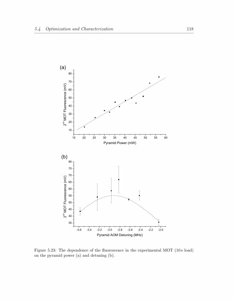
5.4. Optimization and Characterization 118
-3.6 -3.4 -3.2 -3.0 -2.8 -2.6 -2.4 -2.2 -2.0
35
40
45
50
55
60
65
70
75
80
2nd M
OT
Fluo
resc
ence
(mV)
Pyramid AOM Detuning (MHz)
15 20 25 30 35 40 45 50 55 60
10
20
30
40
50
60
70
80
2nd M
OT
Fluo
resc
ence
(mV)
Pyramid Power (mW)
(a)
(b)
Figure 5.23: The dependence of the fluorescence in the experimental MOT (10 s load)on the pyramid power (a) and detuning (b).

5.4. Optimization and Characterization 119
directions. Therefore by observing one direction, it is possible to minimize the
slosh in the other unseen direction. It is crucial to repeat the measurements and
obtain the global minimum, as local minima can occur when slosh in two directions
cancels.
As the CMOT stage causes heating of the cloud, the molasses stage is required
in order to cool the atoms prior to loading the magnetic trap. For the molasses
stage the quadrupole field is turned off, and the shim coils are left on and are
adjusted for a smooth even expansion of the cloud. The optimization of the shim
coil settings is done by sight. There are two infrared cameras observing the MOT
from orthogonal directions, and therefore it is possible to observe the expansion
of the cloud in all directions. The duration of the molasses stage is 15ms. The
optimum duration for the molasses is a balance between increased cooling and
mode-matching the cloud with the magnetic trap.
5.4.5 Optical Pumping
In a MOT, the atoms can be in any magnetic substate (mF ), therefore on loading
the magnetic trap many atoms are lost because of the increased rate of inelastic
collisions. Atoms must therefore be optically pumped into a stretched state. In
this case, the atoms are optically pumped into the F = 3, mF = −3 state.
The atoms are optically pumped into the (3,-3) state by applying a 1.4ms
pulse of circularly polarized light resonant with the 6S1/2, F = 3 → 6P3/2, F′ = 3
transition. The quantization field is produced by the appropriate MOT shim coil
(y-z shim coil). A current of 2.09A is required to produce a field of 2.61G. During
optical pumping the MOT beams are detuned to the 6S1/2, F = 4 → 6P3/2, F′ = 4
transition in order to ensure that no atoms remain in the F = 4 state.
The efficiency of the optical pumping depends on a number of parameters: the
detuning and power of the laser radiation, the pulse length, and the magnitude of
the quantization field. These parameters are all optimized experimentally. Fig-
ure 5.24 illustrates the dependence of the loading efficiency in the magnetic trap
on the detuning of the laser radiation and the pulse length. The measurements

5.4. Optimization and Characterization 120
-15 -10 -5 0 5 10 15 20 255
10
15
20
25
30
35
Per
cent
age
of N
umbe
r of A
tom
s R
ecap
ture
d (%
)
Detuning (MHz)0.0 0.5 1.0 1.5 2.0 2.5 3.0
5
10
15
20
25
30
35
(b)
Per
cent
age
of N
umbe
r of A
tom
s R
ecap
ture
d (%
)
Pulse Length (ms)
(a)
Figure 5.24: Graphs of the percentage of number of atoms recaptured against: (a) thedetuning voltage from the F=3 ↔ F’=3 transition (pulse length = 0.9 ms) and (b) thepulse length (detuning = 2.3 MHz) – for different values of the AOM attenuation: 3.554V(?), 3.94V (¦), 4.4 V () and 4.8 V (•). The dotted line in graph (a) marks the positionof the F=3 ↔ F’=3 transition.
are carried out by noting the fluorescence in the MOT, loading the magnetic trap,
and then recapturing the atoms into the MOT in order to obtain the fluorescence
measurement. The percentage of the number of atoms recaptured is then plotted.
5.4.6 Calibration of Magnetic Trapping Parameters
In order to determine many of the physical quantities such as temperature and
density, it is important to know the parameters of the magnetic trap accurately.
Calibration of the Trap Bias Magnetic Field
The value of the bias magnetic field is determined by measuring the radio-frequency
at which the atoms are expelled from the centre of the trap. To determine this
value accurately, a graph of atom number versus frequency is plotted (Figure 5.25).
Each point on the graph is obtained by varying the end frequency of an evaporation
ramp.
Cutting from both sides of the cloud produces a graph consisting of two lines
which should intersect at y = 0. The rf surface has a finite depth (≈ 10 kHz)
which accounts for a small fraction of the gap seen in Figure 5.25. The majority
of the gap is due to a resonance in the coil at that particular frequency. We

5.4. Optimization and Characterization 121
195 196 197 198 1990.0
0.5
1.0
1.5
2.0
2.5
3.0
Num
ber (
x 1
06 )
Frequency (MHz)
Figure 5.25: Magnetic field calibration. The point at which the straight lines cross the x-axis corresponds to the rf frequency that drives transitions at the bottom of the magnetictrap. The and • correspond to cutting from above and below the cloud respectively.
average the two values of the frequency at y = 0 and using the Breit-Rabi equation
(Equation 2.6), the value of the magnetic field at the bottom of the trap can
be computed. For Figure 5.25 the centre frequency is 196.451(18)MHz which
corresponds to a magnetic field value of 509.870(43) G.
Calibration of the Magnetic Trap Frequencies
It is possible to calculate the field, and therefore the frequencies of the magnetic
trap analytically. However, even when taking into account thickness and curvature
of the baseball coil it is still not possible to determine the trap frequencies more
accurately than within 10 %. The most precise way of determining the magnetic
trap frequencies is by using the atoms.
As mentioned previously, the trap frequencies can be determined from the slosh-
ing frequencies. It is possible to induce sloshing upon loading the magnetic trap
by modifying the trapping potential faster than the atoms can follow. Figure 5.26
is an example of a set of data taken to determine the trapping frequencies. Each

5.4. Optimization and Characterization 122
0 200 400 600 800 1000 1200
202
204
206
208
210
212
214
216
218
220
222A
xial
Cen
tre (p
ixel
)
Time (ms)0 200 400 600 800 1000 1200
320
330
340
350
360
370
380
390
400
410
Rad
ial C
entre
(pix
el)
Time (ms)
Figure 5.26: Determining the frequencies of the magnetic trap. From these plots it ispossible to extract the axial and both radial trap frequencies. The axial trap frequencyis 5.302(19) Hz and the radial frequencies are 12.194(33) Hz and 12.842(40) Hz.
point on the graph represents a single measurement (by imaging) of the positions
of the centre of the cloud in the radial and axial directions. The axial frequency
and both radial frequencies are determined from the plot. The values obtained for
the trap frequencies are 5.302(19) Hz axially, and 12.194(33) Hz and 12.842(40)Hz
radially.
Measurement of the Trap Lifetime
It is important to know the trap lifetime as this can limit the time available to
evaporate and perform experiments.12 The trap lifetime is determined by plotting
the number versus the hold time in the magnetic trap. If an exponential decay is
fitted to the data, the value for the trap lifetime can be extracted. The lifetime
obtained from Figure 5.27 is 537 s (≈ 9 minutes).13
12τb is used in equations to evaluate the two-body and three-body inelastic loss rate coefficients(see Chapter 6).
13This lifetime is long compared to many other alkali metal experiments. We believe thatthe reason for the long lifetime is because initially when the experiment was being built, thevacuum system was baked out three times: initially without the glass cell; then with the glasscell attached; and then a further time as the pyramid mirrors were displaced during moving thevacuum system to the optical table, and therefore the mirrors were repositioned and the systembaked out a final time.

5.4. Optimization and Characterization 123
0 50 100 150 200 250 300 350 40015
20
25
30
35
40
45
Per
cent
age
of n
umbe
r of a
tom
s re
capt
ured
( %
)
Magnetic Trap Hold Duration (s)
Figure 5.27: Determining the magnetic trap lifetime. A plot of percentage of numberof atoms recaptured versus the hold time in the magnetic trap. The line is a weightedexponential fit and gives a value for the trap lifetime of τb = 537 s. (The error bars arethe standard deviation of the data.)

Chapter 6
Loss Measurements
There were two main reasons for studying the magnetic field dependence of inelastic
loss rates in caesium. Inelastic losses play a critical role in determining the success
or failure of evaporative cooling and it is therefore essential to characterize the
losses fully before finalizing the evaporation strategy. Also, due to the work carried
out at Stanford [38] and the subsequent theoretical analysis at NIST [37] we felt
that to characterize these losses experimentally would be of interest, not only to
us but to other research groups studying the collisional properties of caesium.
Initially, the three resonances that occur between 105 and 145G were mapped
out using atomic caesium clouds at a temperature of 250 nK. These resonances had
already been observed by Chu et al. at Stanford [38] and the resonance positions
are therefore confirmed and with reduced uncertainty. The results are given and
discussed in Section 6.2.
In the collisional structure of caesium, Feshbach resonances can show a signifi-
cant shift in position and width with respect to temperature [37]. To demonstrate
this shift experimentally, the resonance centred at approximately 118.5G reso-
nance is plotted for two further temperatures – 80 nK and 800 nK. Theoretical
calculations were also undertaken by Julienne and the results are included and
discussed in Section 6.3.
124

6.1. Inelastic Feshbach Resonances 125
6.1 Inelastic Feshbach Resonances
Resonances are labelled using two quantum numbers, f and l where l is the orbital
angular momentum of the colliding atoms and f is the total hyperfine quantum
number given by f = fa +fb where a and b denote the two colliding atoms individ-
ually. If the entrance and exit channels are identical i.e. (f, l) = (f ′, l′), then the
interaction between the two atoms is due to the exchange forces, whereas if they
are different the interaction is due to relativistic spin-dependent forces.
The scattering in ultra-cold bosonic atomic clouds is purely s-wave. However,
the s-wave entrance channel can couple to higher partial waves (d, g) through
spin-dipolar coupling.1 These resonances tend to be narrow and if the equivalent
higher wave basis2 is not included in the analysis then these resonances are not
theoretically observed.3 The three Feshbach resonances that occur in the (3,−3)
state between 105 and 145G are d-wave resonances.
6.1.1 Comparison of Theoretical and Experimental Data
Generally, the theory quotes the event rate coefficient rather than the collision rate
coefficient. The event rate is the number of inelastic collisions that occur in unit
time and therefore the decay rate of the density n is:
n = −2K2n
The inelastic collision rate (dependent on K2 and K3, and the density) specifies
the number of atoms lost per unit time, therefore the decay rate of the density for
two-body inelastic loss is:
n = −K2n
1Only partial waves of even l are allowed for bosons because of the symmetry of the wave-function.
2In order to observe a d-wave resonance, the d-wave basis functions must be included in thecoupled channel calculations.
3Examples of d-wave resonances are given in Reference [103].

6.2. Feshbach Resonances in the F = 3,mF = −3 State 126
Two atoms are lost in a two-body collision (three atoms are lost in a three-body
collision) therefore K2 is equal to twice the event rate coefficient quoted:
K2 = 2× event rate coefficient
6.2 Feshbach Resonances in the F = 3,mF = −3
State
To determine the two-body inelastic collision rate coefficient K2, the evolution of
the atomic cloud in the magnetic trap must be studied. The magnetic trap is loaded
at 139G from a MOT as described in Chapter 5. After an initial short evaporation
ramp to eliminate all mF states except (3,−3) from the magnetic trap4 we are left
with a pure cloud of approximately 2 × 10⁸ atoms at a temperature of 40 µK.
Forced rf evaporation is then implemented until the temperature of the cloud
reaches approximately 250 nK. The magnetic field is then changed by ramping
the current in the baseball coil to a new value. After variable hold times in the
magnetic trap, images are recorded of the cloud at the field under investigation.
From the resulting computational analysis the number, temperature, and density
as a function of time are obtained.
6.2.1 Determination of the Two-Body Inelastic CollisionRate Coefficient
Under the conditions of our experiment two-body collisions are the dominant in-
elastic loss process in caesium. Therefore for the analysis only two-body collisions
and background collisions are assumed.5 Integrating Equation 4.4 (Chapter 4)
yields an expression for the number of atoms remaining in the trap after time t:
ln(N) +t
τb
= ln(N0)−K2
∫〈n〉dt (6.1)
where N0 is the initial number of atoms in the trap (i.e. the number of atoms at
time t = 0) and 〈n〉 is the mean density. The background loss rate τb, is determined
4All evaporation details are given in Chapter 7.5This is implemented by setting K3 = 0.

6.2. Feshbach Resonances in the F = 3,mF = −3 State 127
separately from data taken at low density (Figure 5.27, Chapter 5), and is therefore
fixed in the analysis (in this case τ = 537 s). The mean density as a function of
time (Figure 6.1 (a) ) is fitted with Equation 6.2.
〈n〉 = y0 + A1 exp (−t/τ1) (6.2)
The time integral of the density in Equation 6.1 is determined by evaluating the
area under the mean density curve (Figure 6.1 (a) ) and is therefore equal to the
integral of Equation 6.2:
∫〈n〉dt = y0t + A1τ1 (1− exp(−t/τ1)) (6.3)
After evaluating Equation 6.2, ln N + t/τb is plotted against time and the
resulting plot is fitted with Equation 6.4.
y = P1 + P2[∫〈n〉dt
]
= P1 + P2 [y0t + A1τ1(1− exp(−t/τ1)] (6.4)
Figure 6.1 is an example of a set of data taken at a single magnetic field. The
dotted curve on the plot (Figure 6.1 (b) ) is a fit of the data assuming three-body
and background collisions (K2=0). This clearly shows that the loss is indeed two-
body in nature under the conditions of our experiment.
6.2.2 Experimental Results
Following the analysis described previously, the value of the two-body inelastic
collision rate coefficient can be plotted as a function of magnetic field. For magnetic
field values between 105 and 150G, three resonances are observed and are plotted
in Figure 6.2.6
The error bars in the plot represent only the uncertainty derived in fitting
the K2 data curve (Figure 6.1 (b) ). Other sources of error, principally in the
determination of the density lead to a larger error in the K2 coefficient (≈ 40%).
The density can vary up to a factor of 10 across the magnetic field range chosen,
6The theoretical prediction is also included on the figure.

6.2. Feshbach Resonances in the F = 3,mF = −3 State 128
0 1 2 3 4 5 6 7 8 9 10
11.0011.2511.5011.7512.0012.2512.5012.75
(b)
(a)
K2 = 3.54(13) x 10-11 cm3s-1
ln N
+ t
/ b
Evolution Time (s)
0 1 2 3 4 5 6 7 8 9 100.0
0.5
1.0
1.5
2.0
Mea
n D
ensi
ty (x
1010
cm-3)
Evolution Time (s)
Figure 6.1: (a) A plot of the measured mean density against the evolution time of thecloud for a magnetic field value of 133.78G. (b) Evaluation of K2. The solid/dottedcurves show the results of a two-/three-body analysis of the data. The scatter in thethe data points indicates the shot-to-shot reproducibility and is the dominant source ofuncertainty.
this in turn affects the inelastic loss rate observed as the losses associated with two-
body collisions are density dependent. This effect is significant for the resonance
centred at 109G as the cloud is ramped across both other resonances before the
hold time in the magnetic trap. This is also true of the temperature – initially
the temperature of the cloud is 250 nK, but ramping the magnetic field across the
resonances can cause the temperature of the cloud to rise by 100 nK.
The centres (position) and widths (FWHM) of each resonance are determined
by performing a weighted fit of a Lorentzian line shape to each of the resonances
individually, allowing for the sloping background associated with a broad resonance

6.2. Feshbach Resonances in the F = 3,mF = −3 State 129
100 110 120 130 140 1501
10
100
1000
K2 L
oss
Coe
ffici
ent (
x 10
-12 cm
3 s-1)
Magnetic Field (G)
Figure 6.2: Two-body inelastic collision rate coefficient for (3,−3) state as a functionof the magnetic field. The dashed curve is the theoretical prediction by Julienne andco-workers [50] at 50 nK with the collisional parameters determined by the Stanforddata [38].
at lower fields:
y = y0 + mx +2A
π
γ
γ2 + 4(x− xc)2(6.5)
The results obtained for the peak positions are given in Table 6.1. The errors of
0.03 to 0.06 G are largely due to the uncertainties in the calibration of the magnetic
field. The FWHM of all three resonances are less than a Gauss. The predictions
of the theoretical model [50] constrained by the data from the Stanford group [38],
and their results [121] for the three resonances at a temperature of 250 nK are also
given in Table 6.1. Our results are in good agreement with the previous experi-
mental results and the theoretical predictions. The difference in errors between the
Stanford data and the theoretical predictions is due to the fact that the theoreti-
cal predictions are made using very precise measurements of only three resonances.
The three resonances discussed in this chapter were not used for the theoretical
predictions. The error in the Stanford measurements of the three resonances used
for the theoretical calculations is 20mG, and therefore the theoretical predictions
cannot quote an error of less than 20mG. The three resonances discussed in this

6.3. Temperature Dependence of the 118.5G Resonance 130
BOxford(G) BStanford(G) BTheory(G)108.87(6) 108.76(20) 108.97(2)118.46(3) 118.05(20) 118.57(2)133.52(3) 133.14(20) 133.48(2)
Table 6.1: Values for the inelastic Feshbach resonances in the (3,−3)× (3,−3) state of apair of atoms between 105 and 135G. The values in the first column are the results fromour experiment in Oxford. Experimental values obtained from Reference [121] are givenin the second column and the third column contains the theoretical values obtained fromReference [50].
chapter were not experimentally characterized as accurately which resulted in an
error of 200mG.
6.3 Temperature Dependence of the 118.5G Res-
onance
Following the characterization of the three resonances, and the good agreement
between the results and the theoretical predictions, it was decided to illustrate
experimentally the dependence of the two-body inelastic collision rate coefficient
on temperature. The magnetic field range chosen was 113 to 125G in order to not
only observe the temperature dependence of K2 off-resonance, but also to observe
the change in width, position and height of the resonance centred at approximately
118.5G.
6.3.1 Experimental Results
The experimental procedure was similar to the procedure used to take the previous
data. For this experiment atom clouds were prepared at temperatures of 80 nK or
800 nK by varying the rf evaporation ramps. The evolution of the cloud at different
magnetic fields was plotted and the data then analyzed to determine K2 for each
temperature at each magnetic field value. Figure 6.3 is a plot of the two-body
inelastic collision rate coefficient for the (3,−3) state in caesium as a function of
magnetic field. The plot consists of data taken at three different temperatures: 80,

6.3. Temperature Dependence of the 118.5G Resonance 131
112 114 116 118 120 122 1241
10
100
1000
K 2 Los
s C
oeffi
cien
t (x
10-1
2 cm3 s-1
)
Magnetic Field (Gauss)
Figure 6.3: Two-body inelastic collision rate coefficient for (3,−3) state as a function ofmagnetic field for three temperatures: 80 nK ( • ), 250 nK ( ), and 800 nK ( ? ). The fitmay appear to be worse for high fields (right hand side of the graph) but this is simply aconsequence of the logarithmic scale. Figure 6.4 contains plots of the resonance for eachindividual temperature on a linear scale.
250, and 800 nK.7
The 80 and 800 nK data contain an increased number of points in order to
improve the accuracy of the fits. This is especially important for the 80 nK data as
it is difficult to reproduce the starting conditions for the measurements accurately
(this is reflected in the magnitude of the error bars). Also, there are no points at
the peak of the 80 nK data because the lifetime of the cloud at the peak is less
than 1 s. Figure 6.4 contains individual plots for each temperature. The error bars
in the plots (Figure 6.3 and 6.4) represent only the statistical uncertainty derived
in fitting the K2 data.
The values obtained for the peak K2, background K2, centre and width of the
resonance at each temperature are given in Table 6.2. As the energy of the collision
7The 250 nK data set is the original loss data measurements (Section 6.2.2) and the relevantdata points from that data set are included in the plot.

6.3. Temperature Dependence of the 118.5G Resonance 132
112 114 116 118 120 122 124 126
0
20
40
60
80
100
K2 L
oss
Coe
ffici
ent (
x 10
-12 cm
3 s-1)
Magnetic Field (G)
112 114 116 118 120 122 124 126
0
100
200
300
K2 L
oss
Coe
ffici
ent (
x 10
-12 cm
3 s-1)
Magnetic Field (G)
112 114 116 118 120 122 124 126
0
100
200
300
400
500
600
K2 L
oss
Coe
ffici
ent (
x 10
-12 cm
3 s-1)
Magnetic Field (G)
(c)
(a)
(b)
Figure 6.4: Two-body inelastic collision rate coefficient for (3,-3) state as a function ofmagnetic field for 80 nK (a), 250 nK (b), and 800 nK (c). (Note: these plots are on alinear scale whereas in Figure 6.3 the scale is logarithmic.)

6.3. Temperature Dependence of the 118.5G Resonance 133
Temperature Position Width Peak K2 K2 at 144G(nK) (mG) (mG) (× 10−12 cm3 s−1) (× 10−12 cm3 s−1)80 118.4822(189) 683(109) 578(104) 13.69(1.58)250 118.4350(62) 726(28) 316(15) 8.94(31)800 118.4538(52) 929(20) 103(3) 3.37(12)
Table 6.2: The table contains the values obtained for the position, width, peak andbackground K2 for the resonance centred at approximately 118.5G. This data is plottedwith the theoretical results [50] in Figure 6.7
increases the magnitude of K2 is greater. The peak K2 is the value of K2 at the
central position of the resonance as determined by the fit (not by the amplitude of
the Lorentzian line shape). The background K2 is the value of the K2 coefficient at
114G (chosen arbitrarily to provide comparison with enhancement at the peak).8
The errors in K2 are principally due to the determination of the density which in
turn leads to a larger error in the K2 coefficient, while the errors in the positions
and widths of the resonance are the statistical uncertainties of the Lorentzian fit.
The errors are discussed in more detail in Section 6.3.3.
6.3.2 Theoretical Results
Following the excellent agreement between the theory and the experimental data
for the three resonances situated between 105 and 150G, Paul Julienne (NIST)
generated data of the inelastic two-body inelastic collision rate coefficient at five
different temperatures and at magnetic field values between 114 and 124G. Fig-
ure 6.5 is a plot of the theoretical data and the results of the fit for the peak K2,
background K2, width, and position of the resonance are given in Table 6.3.
Figure 6.6 is a plot of the theoretical and experimental results of the two-body
inelastic collision rate coefficient for the (3,−3) state in caesium as a function of
8The data is fitted with a Lorentzian line shape allowing for a sloping background, thereforethe background value of K2 is only a guideline.

6.3. Temperature Dependence of the 118.5G Resonance 134
Temperature Position Width Peak K2 K2 at 114G(nK) (mG) (mG) (× 10−12 cm3s−1) (× 10−12 cm3s−1)80 118.4795 704 405(36) 11.7250 118.4661 708 245(20) 6.8500 118.4580 705 166(13) 4.5800 118.4527 702 124(10) 3.31200 118.4482 699 96(7) 2.5
Table 6.3: The table contains the values obtained from the fit of the theoretical data forthe position, width, peak and background K2 for the resonance centred at approximately118.5 G. This data is plotted with the experimental results (Table 6.2) in Figure 6.7.
114 116 118 120 122 124
1
10
100
Even
t Rat
e C
oeffi
cien
t (x
10 -1
2 cm3 s-1
)
Magnetic Field (G)
Figure 6.5: A plot of the theoretical event rate coefficient against magnetic field. Thetheoretical data is fitted with Lorentzian line shapes. The red, green, blue, black andcyan lines correspond to temperatures of 80 nK, 250 nK, 500 nK, 800 nK and 1200 nKrespectively.
6.3. Temperature Dependence of the 118.5G Resonance 135
magnetic field. There is good agreement between the theory and the experimental
results.
The errors quoted for the peak K2 values in Table 6.3 are the statistical errors
associated with the fit. The background K2 is the value of the K2 coefficient at
114G (for comparison with the experimental data). This value is obtained from the
fit and not directly from the theoretical data to allow for direct comparison with
the experimental data. The difference between the two values at each temperature
is no more than 4 %. The error in the width due to the statistical uncertainty
of the Lorentzian fit is no more than 5mG, however the actual error is difficult
to quantify. The theoretical data is constrained by the Stanford data [38] and as
the error in their field calibration is 20 mG, the theoretical data cannot quote an
accuracy greater than 20mG in position. However a more realistic estimate of the
error in position would be 100mG [50].
6.3.3 Experimental and Theoretical Results
Figure 6.6 and Figure 6.7 contain the experimental and theoretical results ob-
tained. The values of the resonance parameters for each individual temperature
have already been stated in Table 6.2 and Table 6.3.
One of the major contributions to the experimental error is the difference in the
initial conditions at each new value of the magnetic field and at each temperature.
After the evaporation and after ramping to a new magnetic field the density of
the cloud is of the order 1010 cm−3. However, the variation in the initial densities
at 80 nK is 18% while at 250 nK and 800 nK the variation is approximately 30%.
This leads to large errors in determining the density and the number. Other
factors that will have an effect on the number of atoms calculated is the variations
in the intensity of the probe laser (I), the detuning of the probe laser (∆), and
any unwanted optical pumping effects that could occur. Also if any atoms are in
magnetic substates other than the (3,−3) state then the inelastic loss rate in the
cloud will be significantly higher.
The error quoted for the width of the resonance is the statistical uncertainty of

6.3. Temperature Dependence of the 118.5G Resonance 136
(c)
112 114 116 118 120 122 124
0.1
1
10
100
K 2 Los
s C
oeffi
cien
t (x
10-1
2 cm3 s-1
)
Magnetic Field (G)
112 114 116 118 120 122 124
1
10
100
K 2 Los
s C
oeffi
cien
t (x
10-1
2 cm3 s-1
)
Magnetic Field (G)
112 114 116 118 120 122 124
1
10
100
K 2 Los
s C
oeffi
cien
t (x
10-1
2 cm3 s-1
)
Magnetic Field (G)
(a)
(b)
Figure 6.6: Two-body inelastic collision rate coefficient for (3,−3) state as a function ofmagnetic field for 80 nK (a), 250 nK (b), and 800 nK (c). The black data points are theexperimental results and the red data points are the theoretical results. (As mentionedpreviously the fit appears inaccurate on the right side of the plot as a consequence ofthe logarithmic scale.)

6.3. Temperature Dependence of the 118.5G Resonance 137
the fit, however the actual error will be greater. As the atom clouds are supported
against gravity with a magnetic field gradient, a large atom cloud will span a large
range of magnetic field values. For example, in a 12Hz trap (radially) a 80 nK cloud
has a FWHM of 30µm. Therefore with a magnetic field gradient of 31 G cm−1 this
leads to a spread of 92mG across the FWHM. For a 800 nK cloud the FWHM
is 93µm and therefore the spread across the cloud is 290mG. This fully explains
the large increase in width (≈ 200mG) observed between the data at 80 nK and
800 nK (Table 6.2 and Figure 6.7).
Another source of error is due to the cloud sloshing in the magnetic trap. Even
though the ramps to new fields should be adiabatic, some sloshing can occur.
Analyzing individual data sets gives a value of 8 pixels for the standard deviation
of the cloud position from the average position. This leads to a magnitude of
≈ 15 pixels for the maximum slosh, which gives a spread in the magnetic field value
of ≈ 600mG, However, many data points are taken at different evolution times at
different magnetic fields and therefore a more realistic value of the maximum slosh
is 4 pixels, giving a spread in the magnetic field of ≈ 150mG.
As the energy of the collision increases the resonance should occur at a smaller
magnetic field. The general trend in Figure 6.7 (c) indicates this, however there is
a discrepancy in the 250 nK data. The 250 nK data was taken a year prior to the
other data, and therefore a change in the calibration of the magnetic field (of the
order of 30mG) could account for this difference.
The results in Figure 6.7 clearly show the dependence of the resonance pa-
rameters on the collision energy. The good agreement between the theory and
the experimental results further confirms the dependence of the two-body inelastic
collision rate coefficient on temperature. The discrepancy in the 250 nK position
data and the increase in the width for the cloud at 800 nK have been accounted
for.

6.3. Temperature Dependence of the 118.5G Resonance 138
(d)(c)
(b)
0 200 400 600 800 1000 1200500
600
700
800
900
1000
Wid
th (m
G)
Temperature (nK)0 200 400 600 800 1000 1200
118.43
118.44
118.45
118.46
118.47
118.48
118.49
118.50
Posi
tion
(Gau
ss)
Temperature (nK)
0 200 400 600 800 1000 1200
23456789
10111213141516
Off-
Res
onan
t K2 (x
10-1
2 cm
3 s-1)
Temperature (nK)0 200 400 600 800 1000 1200
100
200
300
400
500
600
700
On-
Res
onan
t K2 (x
10-1
2 cm
3 s-1)
Temperature (nK)
(a)
Figure 6.7: Graphs illustrating the dependence on temperature of the: peak K2 (a),background K2 (b), position (c), and width (d) of the resonance at 118.5 G.

6.3. Temperature Dependence of the 118.5G Resonance 139
6.3.4 Discussion
The Feshbach resonance at 118G is a d-wave symmetry bound level and therefore
it was believed that only including the s- and d-waves in the coupled channel
calculations was sufficient to obtain accurate characterization of the resonance.
Previously, it had been found that adding g-waves to the basis caused a small shift
in position but little increase in the width of the resonance. However, the original
theoretical data9 did not match our experimental data – the widths were a factor
of three smaller and the background two-body inelastic collision rate coefficient
was also a significant factor smaller. Professor Paul Julienne at NIST has used
his computer code to compare the results of s- and d-wave basis and the s-, d-
and g-wave basis for the resonance we have measured.10 Figure 6.8 illustrates the
results.
114 116 118 120 122 1240.1
1
10
100
Even
t Rat
e C
oeffi
cien
t (x
10 -1
2 cm3 s-1
)
Magnetic Field (G)
Figure 6.8: A comparison of the theoretical results obtained by including s- and d- waves(· · ·) and s-, d- and g-waves (—) in the basis of coupled channel calculations.
At a 114 G the inelastic collision rate associated with g-wave exit channels is
nearly twice that of d-wave channels and therefore including the g-waves gives a
9The original theoretical data only included the s- and d-waves in the basis.10Including the g-waves requires a 74 channel calculation for a single energy and magnetic field
value.

6.3. Temperature Dependence of the 118.5G Resonance 140
value of the event rate coefficient that is nearly three times that of the calculation
including s- and d-waves only. The width of the resonance also increases by ap-
proximately a factor of three.11 The reason why including g-waves had not been
observed to cause such a large effect previously was that fitting specific line shapes
to resonances with such a high degree of precision had not been implemented prior
to this work. It had been noted that the positions were shifted slightly when in-
cluding g-waves but experimental error in the calibration of the magnetic field is
larger than the shift observed in position.
As a result of this work, it has been shown that including g-waves as well as
s- and d- waves in the basis of the coupled channel model is crucial to determine
accurately the line shape of the d-wave resonance centred at 118.5 G. This is likely
to be generally true for all d-wave resonances.
11The widths of these resonances depend sensitively on the second-order spin-orbit operator.

Chapter 7
Evaporation Results
This chapter is devoted to our attempts to condense caesium in the magnetically
trappable F = 3, mF = −3 state. A primary reason for our group to return to
the magnetic trapping of caesium was provided by the more recent observation
and precise measurement of over 25 Feshbach resonances in caesium in several
internal states by the Stanford group [38]. These results accurately determined the
scattering potentials for caesium. Inspection of the predicted collisional properties
for the (3,−3) state indicate that for some bias magnetic field values, caesium
has favourable collisional properties for evaporative cooling, particularly if the
magnetic trap geometry is chosen with care.
Initially, we investigated the evaporative cooling of caesium in a weak magnetic
trap at high bias fields. A PSD within a factor of 10 of the onset of quantum
degeneracy was attained (Section 7.1). The results suggested that the primary
obstacle to the realization of BEC was the reduction in the cooling efficiency as
the gas entered the hydrodynamic regime. The following experiments then focussed
on minimizing the effect of the hydrodynamic regime: by making the evaporation
three-dimensional (Section 7.2), and reducing the scattering length and the two-
body inelastic losses by operating in a very weak trap at a high bias magnetic field
(Section 7.3).
141

7.1. Initial Evaporative Cooling Attempt 142
7.1 Initial Evaporative Cooling Attempt
Taking all the factors affecting the evaporation performance (discussed in Chap-
ter 4) into consideration, the evaporation strategy was to operate in weak magnetic
trapping potentials at high bias fields where the two-body inelastic collision rate
is comparatively favourable [37]. It was decided to load the magnetic trap at
≈ 139G as at this field the ratio of elastic to inelastic collisions was relatively high
and all the resonances were at lower fields (Figure 1.1, Chapter 1). Operating at
a magnetic field higher than the position of all the resonances gave us the option
in future experiments of increasing the magnetic bias field and also weakening the
trap without having to ramp the magnetic field through any resonances.1 A cur-
rent of 234 A is run through the baseball coil generating trap frequencies of 12.2Hz
radially and 5.3 Hz axially. The magnetic field is 139.19 G and the scattering length
is predicted to be 2525 a0.
7.1.1 Experimental Procedure
Upon loading the magnetic trap an initial short high-powered stage of evaporation
is performed in order to expel all atoms in magnetic substates other than mF =
−3 from the trap. Following this stage 2 × 10⁸ atoms at approximately 40 µK
remain in the magnetic trap. To evaporatively cool the atoms, individual stages are
implemented to halve the temperature of the cloud while maximizing the number
of remaining atoms.
The frequency of the rf surface as a function of time f(t) for each evaporation
stage was set to have the form of an exponential decay:
f(t) = fbase + (fstart − fbase)× exp(−t
T
)(7.1)
where
T =−tstage
ln(
fstop−fbase
fstart−fbase
)
1Figure 6.7, Chapter 6 illustrated the dependence of the amplitude of a resonance on collisionenergy. It is therefore advisable not to ramp cold atom clouds through resonances as this increasesthe inelastic loss rate in the cloud, leading to heating and atom loss.

7.1. Initial Evaporative Cooling Attempt 143
Stage fstart fstop fbase tstage Cumulative rf amplit- Tempera-(MHz) (MHz) (MHz) (s) time (s) ude (dBm) ture (nK)
1 55.000 54.200 50.000 15 15 -15 400002 54.200 52.250 50.000 60 75 -25 200003 52.250 51.670 50.500 40 115 -25 100004 51.670 51.125 50.500 25 140 -25 50005 51.125 50.785 50.200 17.5 157.5 -25 25006 50.785 50.538 50.200 11 168.5 -25 10507 50.538 50.405 50.200 7 175.5 -20 4508 50.405 50.330 50.200 3 178.5 -20 2509 50.330 50.270 50.200 2 180.5 -20 10010 50.270 50.245 50.200 1.5 182 -20 5011 50.245 50.227 50.200 1.25 183.25 -20 25
Table 7.1: The evaporation parameters used for the normal evaporation trajectory (biasmagnetic field = 139.2 G).
The four parameters that specify the exponential curve (Equation 7.1) are
the start frequency (fstart), the stop frequency (fstop), the base frequency (fbase),
and the duration of the ramp (tstage). Generally, the start frequency is set to be
the stop frequency of the previous ramp. For the initial ramp after loading the
magnetic trap and for the first evaporation ramp at a different magnetic field,
the start frequency is set to be the resonance frequency of atoms at the edge of
the cloud. The stop frequency is set so that each evaporation stage cooled the
atom cloud by roughly a factor of 2. The base frequency is normally set to be
the resonance frequency of atoms at the centre of the cloud as this means that
the evaporation occurs at constant η. The parameters that are varied in order to
maximize the number of atoms remaining after each stage are: the base frequency
(fbase), the duration of the stage (tstage) and the power of the rf.2 The set of
optimized evaporation ramps is shown in Table 7.1 and plotted in Figure 7.1.
2When varying the base frequency, the duration of the stage, and the rf power, the stopfrequency often needs be altered in order to keep the final temperature equal to half the initialtemperature.

7.1. Initial Evaporative Cooling Attempt 144
0 20 40 60 80 100 120 140 160 18050.0
50.5
51.0
51.5
52.0
52.5
53.0
53.5
54.0
54.5
55.0Fr
eque
ncy
(MH
z)
Time (s)
1 2 3 4 5 6 78
9 1011
Figure 7.1: A plot of the radio-frequency as a function of time. (This is a plot of thevalues in Table 7.1.)
7.1.2 Results
A phase-space density of 0.1 could be reliably achieved, with approximately 1500
atoms cooled to a temperature of 8 nK. The evaporation trajectory, normalized
phase-space density against number, is plotted in Figure 7.2. The ratio of the
increase in PSD (P ) to the fall in number (N) is the evaporative cooling efficiency
denoted by γ:
γ = − d(ln P )
d(ln N)(7.2)
γ is the logarithmic gradient of the trajectory in graphs of PSD against number of
atoms.
Initially the evaporation efficiency (γ) is consistent with other alkali experi-
ments despite our low densities and increased evaporation time (over 3 minutes).
However, as the evaporation progresses the efficiency begins to decrease.
The lines (— and · · ·) on Figure 7.2 indicate the results of a simple rate equa-

7.1. Initial Evaporative Cooling Attempt 145
103 104 105 106 107 10810-7
10-6
10-5
10-4
10-3
10-2
10-1
100
101
Pha
se S
pace
Den
sity
Number
Figure 7.2: A plot of the normalized phase-space density against atom number at a fieldof 139.2G. The results of a simple rate equation model are also shown, with (—) andwithout (· · ·) the hydrodynamic regime. The red curve corresponds to a collision rate of12 Hz. Above this curve the cloud enters the hydrodynamic regime.

7.1. Initial Evaporative Cooling Attempt 146
104 105 106 107 1080
5
10
15
20
Axial Trap Frequency
Elas
tic C
ollis
ion
Rat
e (s
-1)
Number
Radial Trap Frequency
Figure 7.3: A plot of the elastic collision rate against number at a field of 139.2G.
tion model of the evaporation [122]. The solid line includes the hydrodynamic
behaviour by simply smoothly limiting the elastic collision rate to the value of the
trap frequency. The evaporation parameters are then tuned so that the model ap-
proximately matches the evaporation trajectory. The hydrodynamic limit is then
removed from the model while maintaining the same loss terms and evaporation
parameters (dotted line). The dotted trajectory is essentially linear right up to
the BEC transition, despite the large loss terms. The experimentally observed
flattening of the trajectory thus appears to be associated with the hydrodynamic
problem. This conclusion is supported by looking at the evolution of the elastic
collision rate in the gas during evaporation (Figure 7.3). The collision rate in-
creases slowly, becoming comparable to the radial trap frequency between 105 and
106 atoms, precisely where the slope efficiency of the evaporation starts to roll off.3
3Above the red curve on Figure 7.2 the cloud enters the hydrodynamic regime.

7.1. Initial Evaporative Cooling Attempt 147
103 104 105 106 107 10810-4
10-3
10-2D
ecay
Rat
e (s
-1)
Number
Figure 7.4: Individual decay rates during evaporation. The background loss rate ( — ),two-body decay ( • ) and three-body decay ( ).
If we look at the ratio of the elastic collision rate to each of the individual
loss rates (Figure 7.4) we see that initially the evaporation performance is limited
by collisions with the background gas.4 When the number of atoms is between
roughly 4× 10⁵ and 2× 10⁷ the loss rates are dominated by three-body collisions.
As the density falls (Figure 7.5), the three-body losses are reduced due to their
strong dependence on the density and the main loss process is two-body inelastic
collisions.
4Most BEC experiments are limited by background gas collisions in the early stages of evap-oration.

7.2. Two-Frequency Evaporation 148
103 104 105 106 107 108
2
3
4
5
6
7
8
9
Peak
Den
sity
(x 1
010cm
3 )
Number
Figure 7.5: The evolution of the peak density in the atom cloud during evaporation.
7.2 Two-Frequency Evaporation
In Section 2.5.3, Chapter 2 the effect of gravity on the dimensionality of the evap-
oration surface is mentioned. If there were no loss processes in an atom cloud,
one-dimensionality of the evaporation surface would just lead to longer evapora-
tion times. However, in the presence of strong inelastic losses, 1D evaporation
leads to a dramatic reduction in the evaporation efficiency. To study the effects
of dimensionality a second evaporation surface positioned above the centre of the
cloud was introduced. Figure 7.6 illustrates the positioning of the evaporation
surfaces. The top evaporation surface is only in contact with a small area of the
surface of the cloud, whereas the bottom evaporation surface is in full contact with
the cloud. As the bottom evaporation surface is also large it should mean that any
hot diffuse atoms are expelled completely from the trap. Even though the two-
frequency evaporation setup is not fully two dimensional, the results should give
an indication of the effect of dimensionality on the efficiency of the evaporation.
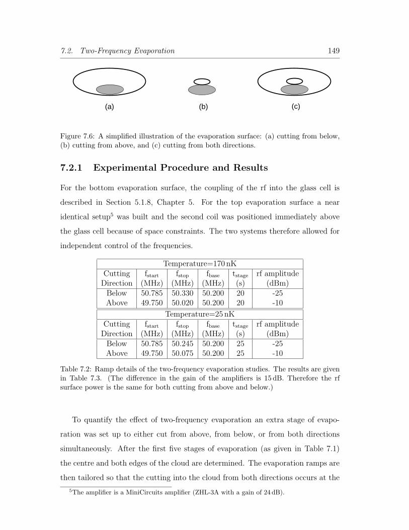
7.2. Two-Frequency Evaporation 149
(a) (b) (c)
Figure 7.6: A simplified illustration of the evaporation surface: (a) cutting from below,(b) cutting from above, and (c) cutting from both directions.
7.2.1 Experimental Procedure and Results
For the bottom evaporation surface, the coupling of the rf into the glass cell is
described in Section 5.1.8, Chapter 5. For the top evaporation surface a near
identical setup5 was built and the second coil was positioned immediately above
the glass cell because of space constraints. The two systems therefore allowed for
independent control of the frequencies.
Temperature=170 nKCutting fstart fstop fbase tstage rf amplitudeDirection (MHz) (MHz) (MHz) (s) (dBm)
Below 50.785 50.330 50.200 20 -25Above 49.750 50.020 50.200 20 -10
Temperature=25 nKCutting fstart fstop fbase tstage rf amplitudeDirection (MHz) (MHz) (MHz) (s) (dBm)
Below 50.785 50.245 50.200 25 -25Above 49.750 50.075 50.200 25 -10
Table 7.2: Ramp details of the two-frequency evaporation studies. The results are givenin Table 7.3. (The difference in the gain of the amplifiers is 15 dB. Therefore the rfsurface power is the same for both cutting from above and below.)
To quantify the effect of two-frequency evaporation an extra stage of evapo-
ration was set up to either cut from above, from below, or from both directions
simultaneously. After the first five stages of evaporation (as given in Table 7.1)
the centre and both edges of the cloud are determined. The evaporation ramps are
then tailored so that the cutting into the cloud from both directions occurs at the
5The amplifier is a MiniCircuits amplifier (ZHL-3A with a gain of 24 dB).

7.2. Two-Frequency Evaporation 150
same rate (equal η) and with the same power. The experiment was undertaken
at two different temperatures: 170 nK and 25 nK. The ramp details are given in
Table 7.2,6 and the experimental results are given in Table 7.3.
Temperature=170 nKCutting Number Temperature PSD PSDDirection (×105) (nK) (×10−3) Ratio
Below 1.72(5) 168(3) 2.63(6) 1Both 1.19(10) 171(6) 1.70(6) 0.65Above 1.56(6) 202(1) 1.35(7) 0.51
Temperature=25 nKCutting Number Temperature PSD PSDDirection (×103) (nK) (×10−3) Ratio
Below 7.43(1.11) 25.5(2.2) 35.6(3.5) 1Both 8.18(0.13) 28.9(4) 24.4(6) 0.68Above 31.8(1.84) 68.6(2.3) 7.1(4) 0.20
Table 7.3: Summary of two-frequency evaporation performance results for an atom cloudat a temperature of 170 nK and 25 nK.
The results clearly illustrate that while cutting from above alone yields poor
evaporation performance, cutting from both above and below simultaneously is still
not as efficient as cutting from below only. At first glance this is a surprise as it is
always assumed that an increase in the dimensionality of the evaporation surfaces
is beneficial. However, further consideration of the trapping geometry, inelastic
two-body collisions and the hydrodynamic regime offer a possible explanation.
7.2.2 Discussion
There are two coupled contributory factors to the efficiency of two-frequency evap-
oration: the hydrodynamic regime and the non-linearity of the Zeeman splitting
at high magnetic fields.
Let us firstly consider the non-linearity of the Zeeman effect. At high magnetic
fields the non-linearity of the Zeeman effect lifts the degeneracy of the transi-
tion frequency between adjacent Zeeman sublevels. The frequency associated with
6The ramp details for cutting from above and below simultaneously are the same as the rampdetails of cutting from above and below individually.

7.2. Two-Frequency Evaporation 151
a particular mF transition is then described by the Breit-Rabi equation (Equa-
tion 2.6, Chapter 2). The ordering of the transition frequencies is given by:
ω−3→−2 > ω−2→−1 > ω−1→0 > ω0→+1 > ω+1→+2 > ω+2→+3 (7.3)
The frequency of the transition from mF = −3 to mF = −2 is 50.148MHz at
139G, which is ≈ 550 kHz larger than the transition from mF = −2 to mF = −1.
This means that atoms can be transferred from mF = −3 to mF = −2 but are
unlikely to be transferred to other states. This can have an adverse effect on the
evaporation efficiency and can completely interrupt the evaporation process [93].
One solution to this problem is to use hyperfine microwave evaporation as in-
corporated in the 7Li experiments [3]. Another solution is to use many different
frequencies tuned to each transition in order to transfer an atom to an un-trapped
state. Boyer et al. condensed 87Rb using a three-frequency rf knife [123]. They
studied the evaporation using a three-frequency rf surface scheme which they sim-
plified to one carrier and two sideband frequencies. This scheme works as 87Rb
has 5 magnetic sublevels therefore three frequencies can transfer an atom from
mF = −2 into an anti-trapped state. The disadvantage of the simplified scheme is
that the two sideband frequencies will not exactly match the transition frequencies.
However the scheme worked well at 56G and resulted in the creation of a BEC
where the standard one-frequency rf knife method had failed [123].
How does the hydrodynamic regime affect the two-frequency evaporation? Three
different scenarios present themselves when considering cutting from above only:
• linear Zeeman effect
• non-linear Zeeman effect
• non-linear effect and large collision cross-section
The best case scenario involves the linear Zeeman effect. By applying the exact
transition frequency an atom undergoes an adiabatic transition from the (3,−3)
state directly to the anti-trapped (3, +3) state. The atom is therefore expelled from

7.2. Two-Frequency Evaporation 152
the trap in random directions and does not necessarily pass through the cloud of
atoms.
At high fields the non-linearity of the Zeeman effect has a large effect on the di-
rection the un-trapped atoms are expelled from the trap. If the difference between
the mF = −3 ↔ −2 and mF = −2 ↔ −1 transition frequency is large enough,
the atoms only undergo Majorana transitions to the mF = −2 state. The spatial
position of the centre of the trap for mF = −2 atoms is lower than mF = −3
atoms, therefore the expelled atoms will fall through the cloud. Under normal
conditions (i.e. many trap oscillations between collisions) it is unlikely that the
mF = −2 atoms would cause an observable detrimental effect.
The final scenario is the worst-case scenario and is the one that we interpret
to be our situation. When trapped atoms that have a large collisions cross-section
encounter the rf surface and undergo Majorana transitions to the mF = −2 state
they have an increased probability of colliding with mF = −3 trapped atoms.
This leads to a dramatic increase in the number of two-body inelastic collisions
occurring in the trapped atom cloud. When cutting from below, the atoms fall
down away from the cloud and therefore neither the non-linearity of the Zeeman
transitions or the large collision cross-section has an effect. When cutting from
above however, both of these effects must be considered as the atoms have an
increased probability of only undergoing Majorana transitions to the mF = −2
state and therefore falling through the cloud. Also, if the cloud has entered the
hydrodynamic regime there is a high probability the un-trapped atom will collide
with trapped atoms while falling through the cloud.
The next question is why cutting from above and below simultaneously is better
than cutting from above only, but worse than cutting from below only?
When cutting from above, the mF = −2 atoms fall through the cloud under-
going collisions with other atoms. However, if an mF = −2 atom were to cross the
cloud without undergoing another collision then it could oscillate past its trapped
position (which is below the mF = −3 trapped position as illustrated in Figure 7.7)
and could travel back into the cloud thus increasing the chance of undergoing an

7.2. Two-Frequency Evaporation 153
-3
-2
-1
Centre of Rf Contours
Sagged Position
Cutting from Below Evaporation Surface
Cutting from Above Evaporation Surface
Figure 7.7: A simplified illustration of the two-frequency principle illustrating the saggedpositions of each magnetically trappable mF state.
inelastic collision with a cold trapped atom. However, if a surface where rf drives
transitions at the bottom of the cloud is present, the mF = −2 atom is unlikely
to succeed in crossing the rf surface on the way out of the cloud and crossing it
again on the way back into the cloud. Figure 7.7 illustrates the position of both rf
surfaces and the positions of all magnetically trappable mF states, taking account
of sagging under gravity.
7.2.3 Heating
To test the hypothesis that hot atoms remain in the trap when cutting from above,
a comparison of cutting from above and below was carried out by observing the
resultant heating rate in the cloud. After completing evaporation stages 1 to 5 (Ta-
ble 7.1) an evaporation stage incorporating cutting from above was implemented.
An equivalent ramp cutting from below was also implemented as a control exper-
iment.7 The ramp parameters for this stage are given in Table 7.4. Following
completion of the extra stage, the rf was turned off and the magnetic trap hold
duration (prior to imaging) was varied. The results are plotted in Figure 7.8.
The results of this experiment (as shown in Figure 7.8) support our hypothesis
that cutting from above is less efficient than from below, and it is this effect that
causes the resulting heating observed in the cloud. When atoms encounter the
7The same coil, amplifier and rf synthesizer was used for both cutting from above and frombelow.

7.2. Two-Frequency Evaporation 154
Cutting fstart fstop fbase tstage rf amplitudeDirection (MHz) (MHz) (MHz) (s) (dBm)
Below 50.785 50.337 50.200 21 -25Above 49.750 50.020 50.200 21 -10
Table 7.4: Details of the cutting from above and below ramp parameters. The resultsare given in Figure 7.8
0 10 20 30 40 50 60150
200
250
300
350
400
450
Tem
pera
ture
(nK
)
Magnetic Trap Hold Duration (s)
Figure 7.8: A plot of the axial temperature of the cloud against magnetic trap holdduration for cutting from above () and below (•) the cloud.
rf surface they undergo Majorana transitions to other states. If they undergo
transitions to mF = −2, −1, and 0, the atoms will fall due to gravity, and if
the evaporation surface is at the top of the cloud, the un-trapped atoms will fall
through the cloud. The presence of other mF states in the cloud causes an increase
in the rate of two-body inelastic collisions, leading to atom loss and an increase in
the temperature of the atom cloud.

7.3. Very Weak Trap 155
7.3 Very Weak Trap
Following the failure to condense caesium at 139.2G and the problems associated
with introducing extra evaporation surfaces, it was decided to evaporate in a very
weak trap and at a higher magnetic field: lowering the trap frequencies delays the
onset of the hydrodynamic regime (Chapter 4), while at higher magnetic fields the
two-body inelastic losses are lower (Figure 1.1, Chapter 1) which was the dominant
loss process later on in the evaporation. Operating at high bias fields where the
scattering length is lower, and reducing the trap frequencies and therefore the
density would also further reduce the three-body inelastic loss rate in the cloud.
7.3.1 Experimental Procedure
To weaken the magnetic trapping potential the baseball current was reduced (Equa-
tion 2.13, Chapter 2). To increase the bias magnetic field, current was run through
the bias coils, adding to the bias magnetic field produced by the baseball coil. Nu-
merical calculations of the trapping potentials suggested that that the lower limit
for the trap frequencies were ≈ 4Hz.8 There is a further constraint on the radial
trapping frequency. The amount of sag is inversely proportional to the square of
the radial trapping frequency (Equation 2.15, Chapter 2), therefore weakening the
trap too much causes the atom cloud to hit the bottom of the glass cell.
The baseball current was reduced from 234A to 209.83 A and the bias current
set to be 232.25A.9 The magnetic field was 510.545(55)G and the measured trap
frequencies at this field were: 4.193(18) Hz radially, and 3.952(16)Hz axially.
The first five stages in the original evaporation strategy have comparable ef-
ficiencies to other BEC experiments, therefore it was decided to continue loading
the magnetic trap at 139.2 G (Labview Baseball Voltage = -3.957V) and perform-
ing stages 1 through 5 prior to moving to the new field. For the early stages of
8If the trap frequencies were reduced further then the potential would no longer trap theatoms.
9The bias current was increased incrementally until a loss in atom number was observedcorresponding to the atom cloud hitting the bottom of the cell. The bias current was then setto be a value slightly lower than the threshold value.

7.3. Very Weak Trap 156
Stage fstart fstop fbase tstage Cumulative rf amplitude(MHz) (MHz) (MHz) (s) time (s) (dBm)
6 198.400 197.450 196.500 30 30 -307 197.450 197.150 196.500 21 51 -308 197.150 196.925 196.500 18 69 -309 196.925 196.750 196.500 16 85 -3010 196.750 196.690 196.500 16 101 -3011 196.690 196.580 196.500 25 126 -30
Table 7.5: Summary of evaporation parameters used in the weak trap, high-field evapo-ration. The evaporation was performed at a magnetic field of 511G and the axial andradial trapping frequencies were 4.0Hz and 4.2 Hz respectively.
evaporation it is crucial to operate in a relatively tight trap as the background loss
rate is the dominant loss mechanism. Following evaporation stage 5 at the original
field, the baseball current was ramped to 209.83A (Labview Baseball Voltage =
-3.500V) and bias current was turned on and increased to a current of 232.25A
(Labview Bias Voltage = -4.000V) in 750ms.10
The evaporation at the new field proceeds as described previously: the tem-
perature is halved while maximizing the number of atoms remaining. The ramp
details for this new field are given in Table 7.5. These stages were performed at
a lower rf amplitude so that the evaporation surface was shallower enabling more
precise cutting.
The atom cloud could not be imaged at the weak field as the position of the
cloud was below the incident position of the probe beam. It was not advisable to
move the probe beam as not only was the position of the atom cloud very close
to the bottom of the glass cell which would lead to diffraction effects and reduce
the resolution of the imaging system, the probe laser was also used to optically
pump the atoms into the (3,−3) prior to loading the magnetic trap. As we were
continuing to load the magnetic trap at 139 G moving the probe beam would
have led to a reduction in efficiency of the optical pumping. The atom cloud was
therefore imaged by ramping the magnetic field back to 139G11 and imaging at
10The ramp duration is determined by studying the heating and number loss following differentramp durations.
11The magnetic field was ramped adiabatically in order to preserve the PSD in the cloud.

7.3. Very Weak Trap 157
the original field.
It was possible to image the atoms without ramping back to the original field
by turning the bias current off and changing the baseball current to 234 A rapidly.
This caused a deformation of the trapping potential and an upwards velocity was
imparted to the atoms. When the atom cloud travelled back into the field of view
it was then imaged. The disadvantage of this method is that information about
the spatial size of the cloud in the weak trap is lost and therefore this method
cannot be used independently. We used both methods in conjunction – we used
the widths obtained from the data taken when the magnetic field was ramped back
to its original value, but the number obtained from the data when the magnetic
field was not ramped back.
7.3.2 Data Analysis
Of course when we image the cloud of atoms that have been evaporated at a high
bias field and weak trap we only obtain information about the collision properties
in the gas at the imaged field. However, by consideration of the scaling laws
of adiabatic compression we can extract the necessary scaling factors in order to
obtain accurate information about the collision rates in the atom cloud in the weak
trapping potential.
During adiabatic compression ω/T is a constant (Chapter 4) and therefore we
can state:
T ′
T=
ω′
ω(7.4)
=ω′2rω
′z
ω2rωz
(7.5)
where the original temperature and geometrical mean of the trap frequencies are
denoted by T and ω respectively, and the temperature and geometrical mean of the
trap frequencies following adiabatic compression by T ′ and ω′ respectively. The
elastic collision rate (Equation 4.1, Chapter 4) can be expressed as follows:
Γelastic =Nω3mσ
π2kBT(7.6)

7.3. Very Weak Trap 158
During adiabatic compression ω/T is constant and therefore the ratio of the
elastic collision rates is given by:
Γ′elastic
Γelastic
=
(ω′
ω
)2σ′
σ(7.7)
When the elastic collision cross-section is independent of temperature Equa-
tion 7.7 becomes trivial. The elastic collision cross-section however, does change
because of the change in scattering length (from 2525 a0 to 1525 a0) and because
of the change in temperature.12 The observed elastic collision rate must therefore
be modified accordingly in order to determine the correct collision rate. The cross-
section is given by Equation 3.23, Chapter 3 and restated here for completeness:
σ =8πa2
1 + k2a2
The ratio of elastic collision rates during adiabatic compression is described by
Equation 7.8:
Γ′elastic
Γelastic
=
(ω′
ω
)2 (a′
a
)21 + (ka)2
1 + (k′a′)2(7.8)
Normal Trap Weak Trap139G 511G
Radial frequency ωr 2π × 12.194 2π × 4.193Axial frequency ωz 2π × 5.302 2π × 3.952
Scattering Length a 2525 a0 1525 a0
Table 7.6: Summary of the trap parameters and scattering length in the normal trap (at139 G) and in the weak trap (at 511 G).
Using the values given in Table 7.6 and the fact that ω/T is a constant during
adiabatic compression it is possible to obtain an expression for the ratio of the
elastic collision rates:
Γ′elastic
Γelastic
=0.0722 (1 + 25.1114 T )
1 + 4.07629 T(7.9)
where T is the temperature of the cloud at the imaged field.
12The collisional cross-section in caesium is temperature dependent.

7.3. Very Weak Trap 159
103 104 105 106 107 108
10-7
10-6
10-5
10-4
10-3
10-2
10-1
100Ph
ase
Spac
e D
ensi
ty
Number
Figure 7.9: Evaporation trajectory for 133Cs atoms trapped in 12 × 12 × 5 Hz ( • ) and4 × 4 × 4 Hz ( ) magnetic traps. The solid curves show the results of the simulation[52] for 180 s of evaporative cooling. The red and green curves correspond to a collisionrate of 12 Hz (12×12×5Hz trap) and 4 Hz (4×4×4Hz trap) respectively. Above thesecurves the cloud enters the hydrodynamic regime
7.3.3 Results
To compare accurately the original evaporation trajectory and the very weak trap
results,13 the data points are taken alternately from the original evaporation ramps
(Table 7.1) and the new evaporation ramps (Table 7.5). The data is plotted in
Figure 7.9.
Weakening the trap clearly improves the end PSD attained by a factor of three,
however there is still a roll-off in the performance of the evaporation. Figure 7.10
illustrates the evolution of the elastic collision rate during the evaporation. The
flattening of the trajectory in Figure 7.9 happens later on in the evaporation for a
13The original evaporation trajectory (Figure 7.2) was taken a year previously and thereforeit was decided to repeat the measurements in order to obtain an accurate indication of the weaktrap evaporation performance.

7.3. Very Weak Trap 160
weak trap (compared to the original evaporation trajectory in Figure 7.2), but we
are still unable to reach a PSD of 1.
103 104 105 106 107
1.5
2.0
2.5
3.0
3.5
4.0
4.5
Axial Trap Frequency
Radial Trap Frequency
Elas
tic C
ollis
ion
Rat
e (s
-1)
Number
Figure 7.10: A plot of the elastic collision rate against number at a field of 510.5 G. (Thecollision rate was scaled as described in Section 7.3.2.)

7.3. Very Weak Trap 161
7.3.4 Discussion
Following the failure to condense caesium at 139G and 510G it was decided to
try and simulate the evaporation and determine what, if any, parameter could be
varied in order to improve the evaporation performance [124].14 In Figure 7.9, the
simulation accurately reproduces the experimental results. Both the experimental
data and the simulation result show that the evaporation performance is slightly
improved if the trap frequencies are weakened. Also, the results show a decrease
in the efficiency of the evaporation as the cloud enters the hydrodynamic regime.
To investigate the detrimental effect of entering the hydrodynamic regime on
the evaporation performance, simulations were performed on atom clouds with
different initial phase-space densities. Even when the initial PSD (after stage 1)
was varied by a factor of 10, the evaporative cooling curves all cross one another
when the cloud enters the hydrodynamic regime (Figure 4 (b) in Reference [52]).
The duration of the evaporation was varied experimentally and the evaporation
trajectory simulated in order to determine whether the duration was optimum. To
vary the total duration of the evaporation, the individual ramp durations were
scaled accordingly.15 Figure 7.11 illustrates the result of varying the evaporation
time experimentally and theoretically. The evaporation performance is not very
sensitive to the evaporation duration, although there is an optimum value (in the
simulation) of around 150 s in a 12× 12× 5Hz trap.
Another important factor in the evaporation performance is the dimensionality
of the evaporation surface. The simulation results for one-dimensional cutting from
one side of the cloud, one-dimensional cutting from both sides of the cloud16 and
three-dimensional cutting in a 12Hz spherical trap were compared. The results
suggested that BEC could be realized with three-dimensional cutting [52].
14The simulation was performed by Z.-Y. Ma and the full results are published in Reference [52],while the relevant simulations for the experimental results are included in Figure 7.9 and 7.11.
15Ramp 1 was not modified as its function is to remove other mF states, and is therefore notpart of the evaporation.
16Equivalent situation as the experimental setup explained in Section 7.2.

7.3. Very Weak Trap 162
50 100 150 200 250 300 350 400 450 50010-4
10-3
10-2
10-1
Pha
se S
pace
Den
sity
Duration (s)
Figure 7.11: The final phase space density as a function of the evaporation time in a12× 12× 5Hz trap: experiment ( • ) and simulation ( )
We achieved a PSD of 0.3 which is a factor of 10 higher than previous Cs
experiments in the magnetically trappable states (Table 4.2, Chapter 4). This
increase was achieved by careful consideration of the ratio of elastic to inelastic
collisions in various loss regimes and by delaying the onset of the hydrodynamic
regime by operating in weak magnetic traps.
The three main factors that conspire to decrease the efficiency of the evapora-
tion and ultimately the failure to condense caesium in the magnetically trappable
F = 3,mF = −3 state are: the onset of the hydrodynamic regime, the high rate
of two-body inelastic losses and the dimensionality of the evaporation surface.
Chapter 8
Conclusion
We have evaporatively cooled a magnetically trapped sample of caesium atoms
in the F = 3,mF = −3 state to a PSD within a factor of four of the BEC
transition, which is at least ten times higher than previous magnetically trapped
caesium experiments. We have shown that previous experiments did not work
because the cloud of trapped atoms was in the hydrodynamic regime. The increase
in the PSD that we achieved was due to careful consideration of the optimum
conditions for evaporative cooling. We operated with a weak magnetic trap at
high magnetic fields to reduce the two-body inelastic loss rates and delay the onset
of the hydrodynamic regime in the evaporative cooling stage.
A numerical simulation of evaporative cooling was developed that accurately
reproduced our experimental observations [124]. The simulation results indicated
that the main obstacle to the realization of quantum degeneracy in the (3,−3)
state was the reduction in the evaporative cooling efficiency in the hydrodynamic
regime.
A lower dimensionality of the evaporation surface was also detrimental to the
cooling efficiency. The effects of the non-linearity of the Zeeman effect and the
presence of extra evaporation surfaces was studied and it was observed that at
high magnetic fields and when the cutting surface is above the atom cloud the
evaporation is less efficient.
163
8.1. Outlook 164
During the course of this work we have characterized the two-body losses at
magnetic fields ranging from approximately 105 to 150G, confirming the positions
of three previously identified resonances [38] and the validity of theoretical predic-
tions [37]. We have also studied the dependence of two-body inelastic loss rates on
the collisional energy. The resonance centred at 118.5G was plotted at three dif-
ferent temperatures and the widths, position, peak and background K2 compared
for each temperature. The results indicate that with increasing collision energy
the two-body loss rate decreases both on and off-resonance. The position of the
resonance occurs at higher fields for decreasing collisional energy. The results are
in good agreement with the theoretical predictions [50].
The importance of including g-waves in the basis of the theoretical analysis was
realized during the course of this work. Previously it was thought that including
s and d exit channels in d-wave resonance calculations was sufficient to accurately
determine the shape and position of the resonance. Following our work in fitting a
specific shape to a resonance with a high level of precision, theoretical calculations
were undertaken by Julienne at NIST which included the g-wave exit channels for
the d-symmetry resonance level. He discovered that including the g-waves in the
analysis shifted the position of the resonance slightly, changed the K2 value both
on and off-resonance and significantly changed the width of the resonance.
8.1 Outlook
Is it possible to condense caesium in the (3,−3) state? By analyzing the limitations
of the present experiment there are a few changes that could be made to improve
the evaporative cooling efficiency.
Reference [52] states that condensing caesium in the magnetically trappable
state is possible if the evaporation is three dimensional. However, in order to
avoid the hydrodynamic regime, evaporation must take place in weak magnetic
trap and therefore gravity will always make the evaporation one-dimensional. One
improvement would be to operate in a pancake shape trap (very tight in the vertical
direction and weak in the other two directions). This would not only reduce the

8.1. Outlook 165
gravitational sag but the evaporation surface would be very large and would be
in full contact with the bottom of the cloud thus reducing the hydrodynamic
problem. Unfortunately it is impossible to generate a weak trapping potential
in two directions while maintaining a strongly confining potential in the third
direction in a baseball trap. Varying the current to the baseball coil changes all
three trapping frequencies. The bias coils permit modification of the trapping
frequencies but once again all three directions are inter-dependent. The only trap
that allows complete independent control of each trapping frequency is the clover-
leaf trap [83]. Also the design of the cloverleaf allows significantly better optical
access1 to the trapped atoms than that available with the baseball and bias coils.
Such modifications would improve the efficiency of the evaporative cooling, but
it is unknown as to whether this factor would be enough to observe BEC.
BEC has been achieved in caesium in the (3, +3) state and the advantages of
operating in this state are obvious. The greatest versatility to control BEC interac-
tions exist as there is a large broad Feshbach resonance between 0 and 50G where
the scattering length changes from negative to positive. The scattering length
is zero at 17 G leading to the possibility of study of non-interacting condensates.
There exists a narrow Feshbach resonance at a higher magnetic field (48G) which
allows for the creation of molecules. Both of these resonances occur at magnetic
fields that are experimentally easy to access. Also in the Innsbruck experiment
the bias magnetic field can be changed without altering the trap frequencies (Ap-
pendix A).
Why therefore would it be of benefit to work with caesium in the (3,−3) state?
There are many experiments involving cold atoms, but not necessarily a BEC, that
could be carried out using a caesium atom cloud.
The hydrodynamic regime is an area of collisional physics that is not very well
understood. Caesium is well suited to hydrodynamic regime studies because of
its large scattering length, therefore the entry of the cloud into the hydrodynamic
regime is almost unavoidable.
1The cloverleaf trap allows 360 optical access.

8.1. Outlook 166
To observe quantum tunnelling effects a BEC is normally loaded into and op-
tical lattice. However, the temperatures that can be attained by evaporatively
cooling caesium is much lower than the critical temperatures for all other BEC
experiments. It could therefore be interesting to load an extremely cold caesium
atom cloud (less than 50 nK) into an optical lattice and compare the resulting
effects with a BEC loaded into an equivalent lattice.
The scattering properties of Cs in many internal states has been studied in
detail [37, 38], and both the (3,−3) and the (3, +3) state posses collisional fea-
tures that are not only experimentally but also theoretically interesting. Both
states contain Feshbach resonances that are experimentally accessible. A wealth
of physics has opened up due to the ability to use Feshbach resonances to tune
inter-atomic interactions: molecules are created, collision gates in quantum com-
puting manipulated, and the collapse and revival of condensates studied. Caesium
is one of the most versatile alkali metals and its cold collision properties holds great
prospects for future research in the field of quantum gases.
Appendix A
Bose-Einstein Condensation inCaesium
A Bose-Einstein condensate of caesium atoms was created on the 5th of October,
2002 in Innsbruck [12]. Grimm et al. achieved BEC by evaporative cooling using
optical trapping techniques. This appendix is a summary of their experiment and
illustrates how they achieved BEC and the difficulties they overcame along the
way.
The F = 3, mF = +3 state in caesium is the lowest internal state and therefore
the absence of internal energy leads to full suppression of inelastic two-body loss.
Therefore the important loss rates in the trap are due to background gas collisions,
three-body collisions, and photon scattering from the dipole trap.1
A.1 Experimental Setup
The initial experimental procedure is similar to other alkali metal experiments.
Following cooling in the MOT and an optical molasses stage, approximately 108
atoms at a temperature of 10 µK are loaded into an optical lattice. Raman sideband
cooling is then implemented to both cool and polarize the atoms [40]. 2×10⁷ atoms
at a temperature of 1µK are then loaded into an optical trap by adiabatic release
of the atoms from the optical lattice.
1The large laser detuning from resonance of the CO2 beams results in a negligibly smallphoton scattering rate.
167

A.2. Evaporation 168
The optical trap is based on a crossed-beam CO2 trap . Each beam is generated
by a 100W CO2 laser and the beams cross at 90 (Figure A.1 (a) ). A magnetic
levitation field to support the atoms against gravity is essential as the optical
forces in the CO2 trap are much lower than the gravitational force. A levitation
trap (LEVT) is created by generating a magnetic gradient using a pair of coils in
an anti-Helmholtz configuration [1, 41]. A combination of the optical trap and the
LEVT results in a shallow large volume trap which can be loaded with a large
number of atoms.2 The effective volume is approximately 1mm3, the trap depth
is 10µK, and the geometrical mean of the trap frequencies is 14Hz.
(a) (b) (c)
Figure A.1: An illustration of the setup of the laser beams in the Innsbruck experiment:(a) the crossed-beam CO2 trap, (b) loading the “dimple” trap, and (c) evaporation inthe “dimple” trap. This figure is modified from Reference [12].
An extra pair of coils in a Helmholtz arrangement is used to tune the bias
magnetic field. This results in the bias magnetic field value being freely adjustable
without altering the trap frequencies, and therefore B0 is a free parameter.
A.2 Evaporation
Initially, evaporation proceeds on loading the CO2 trap.3 For 10 s, atoms are evap-
orated out of the trap at a constant trap depth, resulting in a cloud of 3 × 10⁶
2The LEVT cancels gravity for the (3,+3) state and as the optical trapping forces are so weakno other mF states are supported against gravity. This results in a pure (3,+3) atom cloud inthe optical trap.
3On loading the CO2 trap the scattering length is chosen to be 1200 a0 (at 75 G) in order toobtain a sufficient collision rate in the atom cloud.

A.2. Evaporation 169
atoms at a temperature of 1 µK (PSD ≈ 10−3). Forced rf evaporation is then im-
plemented, but because of the vertical levitation gradient the rf surface is only
resonant with atoms at the bottom of the cloud leading to one-dimensional evap-
oration. They achieved a PSD of 0.3 with 2500 atoms remaining.
In their initial work the achievement of Bose-condensation was prevented by
three-body recombination. Theory predicts that the three-body loss rate scales as
a4 [125] and a large scattering length therefore leads to a large loss in number and
heating. In three-body recombination a diatomic molecule forms from two of the
atoms and the third one takes away the binding energy of the molecule. In a deep
trap this third atom remains in the trap causing heating. A shallower trap allows
the third atom to escape. Grimm et al. then implemented three improvements:
optimization of the trap depth and the scattering length, implementing efficient
three-dimensional evaporation, and avoiding the hydrodynamic regime.
kBT
Udimple
(b)(a)
Figure A.2: An illustration of the principle of the “dimple” trap.
Deforming the trapping potential can result in an increase in PSD without a loss
in number [126]. Grimm et al. created a narrow and deep potential well [127] in the
center of the CO2 trap by focussing a beam of wavelength 1064 nm, produced by an
Ytterbium fibre laser, into the sample. Figure A.1 (b) illustrates the positioning of
the 1064 nm beam in the CO2, and Figure A.2 illustrates the resulting potential.
The adiabatically deformed potential (called the “dimple” trap) results in a large
gain in PSD as the density in the trap is greatly increased.4 The new PSD (P ) is
4The temperature in the atom cloud does increase slightly but the effect is negligible comparedto the increase in the density.
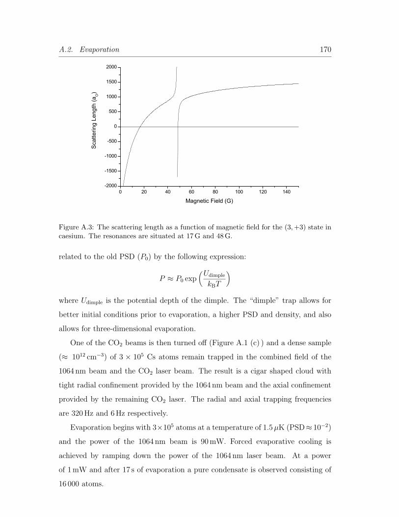
A.2. Evaporation 170
0 20 40 60 80 100 120 140-2000
-1500
-1000
-500
0
500
1000
1500
2000
Sca
tterin
g Le
ngth
(aO)
Magnetic Field (G)
Figure A.3: The scattering length as a function of magnetic field for the (3, +3) state incaesium. The resonances are situated at 17 G and 48 G.
related to the old PSD (P0) by the following expression:
P ≈ P0 exp(
Udimple
kBT
)
where Udimple is the potential depth of the dimple. The “dimple” trap allows for
better initial conditions prior to evaporation, a higher PSD and density, and also
allows for three-dimensional evaporation.
One of the CO2 beams is then turned off (Figure A.1 (c) ) and a dense sample
(≈ 1012 cm−3) of 3 × 10⁵ Cs atoms remain trapped in the combined field of the
1064 nm beam and the CO2 laser beam. The result is a cigar shaped cloud with
tight radial confinement provided by the 1064 nm beam and the axial confinement
provided by the remaining CO2 laser. The radial and axial trapping frequencies
are 320 Hz and 6Hz respectively.
Evaporation begins with 3×10⁵ atoms at a temperature of 1.5 µK (PSD≈ 10−2)
and the power of the 1064 nm beam is 90 mW. Forced evaporative cooling is
achieved by ramping down the power of the 1064 nm laser beam. At a power
of 1mW and after 17 s of evaporation a pure condensate is observed consisting of
16 000 atoms.

A.3. Comparison 171
The creation of a BEC of caesium was achieved at a bias magnetic field of 23G
(a = 300 a0). It was only possible to condense at magnetic fields between 21 and
25G. Below 21 G the elastic collision cross-section was too small, whereas for mag-
netic fields greater than 25 G the increase in scattering length leads to an increase
in three-body collisions and the entry of the cloud into the hydrodynamic regime.
Figure A.3 illustrates the resonance structure of the (3,+3) state in caesium.
A.3 Comparison
Even though the Oxford and Innsbruck experiments operate in different traps and
magnetic states, both face similar problems. One-dimensional evaporation is an
inherent problem in both traps and the temperature dependence of the elastic
collisional cross-section leads to an increase in the rethermalization time. The
main difference between both experiments is the magnetic states that are trapped.
Innsbruck trap the (3, +3) state which is the stable against two-body inelastic colli-
sions, whereas in Oxford the (3,−3) state is trapped magnetically. Their dominant
collisions are three-body recombination whereas our dominant loss process is due
to two-body inelastic collisions.
Figure A.4 illustrates our results and the experimental results of the caesium
experiment at Innsbruck. Their original results with one-dimensional evaporation
are comparable to our results, and it is only when they implemented efficient
three-dimensional evaporation that they succeeded in Bose-condensing Cs.5
5In the summer of 2002 there were many conferences at which both experiments were rep-resented. This lead to many collaborative discussions about the problems in each experiment.We were already trying to implement a three-dimensional evaporation scheme. It is difficult toimplement three-dimensional evaporation successfully in a magnetic trap, however it was possiblein an optical trap to implement the “dimple” trap to allow three-dimensional evaporation.

A.3. Comparison 172
103 104 105 106 107 10810-7
10-6
10-5
10-4
10-3
10-2
10-1
100
1D 3D
Phas
e Sp
ace
Den
sity
Number
Figure A.4: The evaporation trajectory for 133Cs atoms in our magnetic trap at Oxford(from Figure 7.9) and the optical trap at Innsbruck. The Innsbruck results are denotedby ? (one-dimensional evaporation) and ¦ (three-dimensional evaporation).

Appendix B
Experimental Equipment Details
B.1 Computer Control Boards
The computer boards are from ‘National Instruments’. The control computer
contains three different boards (see below) which are all controlled by the Labview
software program.
PCI-GPIB A high-performance GPIB interface. The rf values from the Labview
control program to the frequency-generator are transferred via GPIB.
PCI-6713 A 12-Bit, 1 MS/s per channel analog output board. It consists of 8
analogue channels and 8 digital channels. The analogue channels are used
for the magnetic trap Labview input voltages (Figure 5.14, Chapter 5).
PCI-DIO-32HS A high-speed pattern I/O and handshaking board. This board
consists of 32 digital outputs and it generates the TTL signals required to
control the experiment.
173
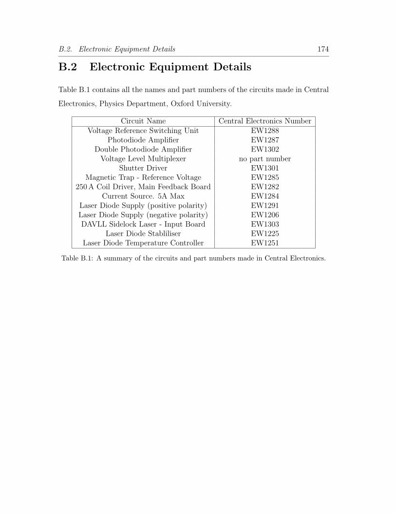
B.2. Electronic Equipment Details 174
B.2 Electronic Equipment Details
Table B.1 contains all the names and part numbers of the circuits made in Central
Electronics, Physics Department, Oxford University.
Circuit Name Central Electronics NumberVoltage Reference Switching Unit EW1288
Photodiode Amplifier EW1287Double Photodiode Amplifier EW1302
Voltage Level Multiplexer no part numberShutter Driver EW1301
Magnetic Trap - Reference Voltage EW1285250A Coil Driver, Main Feedback Board EW1282
Current Source. 5A Max EW1284Laser Diode Supply (positive polarity) EW1291Laser Diode Supply (negative polarity) EW1206DAVLL Sidelock Laser - Input Board EW1303
Laser Diode Stabliliser EW1225Laser Diode Temperature Controller EW1251
Table B.1: A summary of the circuits and part numbers made in Central Electronics.

Appendix C
Caesium Atomic Data andExperimental Equations
C.1 Atomic Parameters
Name Symbol Value UnitResistivity ρE 1.72×10⁻⁸ ΩmDensity ρ 8920 kgm−3
Specific heat of copper C 3.9×10² J kg−1 K−1
Specific heat of water C 4.2×10³ J kg−1 K−1
Wavelength λ 852 nmNatural linewidth of 6P3/2 Γ 2π× 5.22 MHzSaturation intensity for IS 1.1 mWcm2
6S1/2|4, 4 >−→ 6P3/2|5, 5 >Nuclear Spin I 7/2
∗ Nuclear Gyromagnetic Ratio gI 0.00039885395(52)† Electron Gyromagnetic Ratio gJ 2.0023193043718(75)
Ground State Hyperfine Splitting υHFS 9.192631770 ×10⁹ GHz
Table C.1: ∗ and † constants obtained from Reference [128] and [129] respectively.
C.2 Magnetic Field Calculations
The on-axis field produced by a single coil of radius R is given by:
Bz =µ0
2
nIR2
(A2 + R2)32
(C.1)
175

C.3. Number of Atoms 176
where n is the number of turns, I is the magnitude of the current flowing through
the coil, and A is the distance along the axis of the coil from the centre
The field gradient for a pair of coils in an anti-Helmholtz arrangement with
with radius R and separation 2A is given by:
∂B
∂z
∣∣∣∣∣z=0
=3nIR2Aµ0
(A2 + R2)52
(C.2)
For the experimental setup described in the thesis, Table C.2 states all the
relevant parameters of the quadrupole and shim coils.
Number Dimensions Separation / Distan- Bof Turns (cm) ce from atoms (cm) ( G cm−1 )
Pyramid Quad 15 R = 5.6 2A = 5 0.51G/cm/APyramid Shim 100 R = 7.8 A = 10 1.87G/A
2nd MOT Quad 80 R = 2.5 2A = 7 4.48G/cm/A2nd MOT Shim 50 R = 18 A = 9 1.25G/A
Table C.2: A summary of the magnetic coil parameters on the experiment
C.3 Number of Atoms
The number of atoms in a MOT can be calculated from the fluorescence measure-
ment [68]. A summary of the required equations are given below.
The power radiated by an atom in a MOT is given by:
Pat =hωLΓ
2
C21Ω2
tot/2
δ2 + Γ2/4 + C22Ω2
tot/2(C.3)
where
Ω2tot =
Γ2
2
I
Is
(C.4)
The constants C1 and C2 are determined experimentally [68]:
C21 = C2
2 = 0.73(10)
Substituting Equation C.4 into Equation C.3 yields the result:
Pat =hωLΓ
2
C21I/Is
1 + C22I/Is + 4δ2/Γ2
(C.5)

C.3. Number of Atoms 177
The power incident on the photodiode is:1
P = NPatΩ
4π(C.6)
where Ω is the solid angle subtended by the collection lens and is equal to
πd2
4x2(C.7)
d is the diameter of the collection lens and x is the distance from the atoms to the
collection lens.
The light incident on the photodiode gives rise to a signal S given by:
S(V ) = PR(λ)Rload (C.8)
where R(λ) is the responsivity of the photodiode and Rload is the load resistance.
Combining Equations C.7 and C.8, we obtain the following expression for N:
N =S(V )
R(λ)Rload
16x2
d2
1
Pat
(C.9)
where Pat is as stated in Equation C.5.
1Due to the limited solid angle of the collection optics the power incident on the photodiodeis a fraction of the actual power radiated by the atoms.

Bibliography
[1] M. H. Anderson, J. R. Ensher, M. R. Matthews, C. E. Wieman,
and E. A. Cornell, “Observation of Bose-Einstein condensation in a di-
lute atomic vapor”, Science 269, 198 (1995).
[2] K. B. Davis, M.-O. Mewes, M. R. Andrews, N. J. van Druten,
D. S. Durfee, D. M. Kurn, and W. Ketterle, “Bose-Einstein con-
densation in a gas of sodium atoms”, Phys. Rev. Lett. 75, 3969 (1995).
[3] C. C. Bradley, C. A. Sackett, J. J. Tollett, and R. G. Hulet,
“Evidence of Bose-Einstein condensation in an atomic gas with attractive
interactions”, Phys. Rev. Lett. 75, 1687 (1995), ibid. 79 , 1170 (1997) .
[4] S. L. Cornish, N. R. Claussen, J. L. Roberts, E. A. Cornell,
and C. E. Wieman, “Stable 85Rb Bose-Einstein condensates with widely
tunable interactions”, Phys. Rev. Lett. 85, 1795 (2000).
[5] S. Jochim, M. Bartenstein, A. Altmeyer, G. Hendl, S. Riedl, C.
Chin, J. H. Denschlag, and R. Grimm, “Bose–Einstein condensation
of molecules”, Science 302, 2101 (2003).
[6] M. Zwierlein, C. Stan, C. Schunk, S. Raupach, S. Gupta, Z. Hadz-
ibabic, and W. Ketterle, “Observation of Bose–Einstein condensation
of molecules”, Phys. Rev. Lett. 91, 250401 (2003).
[7] D. Fried, T. Killian, L. Willmann, D. Landhuis, S. Moss, D.
Kleppner, and T. Greytak, “Bose-Einstein condensation of atomic hy-
drogen”, Phys. Rev. Lett. 81, 3811 (1998).
178

BIBLIOGRAPHY 179
[8] A. Robert, O. Sirjean, A. Browaeys, J. Poupard, S. Nowak, D.
Boiron, C. I. Westbrook, and A. Aspect, “A Bose-Einstein conden-
sate of metastable atoms”, Science 292, 461 (2001).
[9] F. P. D. Santos et al., “Bose-Einstein condensation of metastable helium”,
Phys. Rev. Lett. 86, 3459 (2001).
[10] G. Modugno, G. Ferrari, G. Roati, R. J. Brecha, A. Simoni, and
M. Inguscio, “Bose-Einstein condensation of potassium atoms by sympa-
thetic cooling”, Science 294, 1320 (2001).
[11] C. Regal, M. Greiner, and D. Jin, “Observation of resonance conden-
sation of fermionic atom pairs”, Phys. Rev. Lett. 92, 040403 (2004).
[12] T. Weber, J. Herbig, M. Mark, H.-C. Nagerl, and R. Grimm,
“Bose-Einstein condensation of cesium”, Science 299, 232 (2003).
[13] S. Bose, “Plancks Gesetz und Lichtquantenhypothese”, Z. Phys. 26, 178
(1924).
[14] A. Einstein, “Quantentheorie des einatomigen idealen Gases. Zweite Ab-
handlung”, Sitzungber. Preuss. Akad. Wiss. 1925, 3 (1925).
[15] M.-O. Mewes, M. R. Andrews, D. M. Kurn, D. S. Durfee, C. G.
Townsend, and W. Ketterle, “Output coupler for Bose-Einstein con-
densed atoms”, Phys. Rev. Lett. 78, 582 (1997).
[16] S. Inouye, M. R. Andrews, J. Stenger, H.-J. Miesner, D. M.
Stamper-Kurn, and W. Ketterle, “Observation of Feshbach reso-
nances in a Bose-Einstein condensate”, Nature 392, 151 (1998).
[17] J. L. Roberts, N. R. Claussen, S. L. Cornish, E. A. Donley, E. A.
Cornell, and C. E. Wieman, “Controlled collapse of a Bose-Einstein
condensate”, Phys. Rev. Lett. 86, 4211 (2001).

BIBLIOGRAPHY 180
[18] E. Donley, N. Claussen, S. Cornish, J. Roberts, E. Cornell,
and C. Wieman, “Dynamics of collapsing and exploding Bose-Einstein
condensates”, Nature 412, 295 (2001).
[19] E. Donley, N. Claussen, S. Thompson, and C. Wieman, “Atom-
molecule coherence in a Bose-Einstein condensate”, Nature 417, 529 (2002).
[20] M. Greiner, C. Regal, and D. Jin, “A molecular Bose–Einstein con-
densate emerges from a Fermi sea”, Nature 426, 537 (2003).
[21] K. Gibble and S. Chu, “Future slow–atom frequency standards”, Metrol.
29, 201 (1992).
[22] P. Julienne and F. Mies, “Collisions of ultracold trapped atoms”, Phys.
Rev. A 6, 2257 (1989).
[23] E. Tiesinga, A. Moerdijk, B. J. Verhaar, and H. T. C. Stoof,
“Conditions for Bose-Einstein condensation in magnetically trapped atomic
cesium”, Phys. Rev. A 46, R1167 (1992).
[24] J. Soding, D. Guery-Odelin, P. Desbiolles, G. Ferrari, and J.
Dalibard, “Giant spin relaxation of an ultracold cesium gas”, Phys. Rev.
Lett. 80, 1869 (1998).
[25] M. Arndt, M. B. Dahan, D. Guery-Odelin, M. W. Reynolds, and
J. Dalibard, “Observation of a zero-energy resonance in Cs-Cs collisions”,
Phys. Rev. Lett. 79, 625 (1997).
[26] P. Bance, Evaporative Cooling of Caesium in a TOP Trap: Prospects for
BEC, Ph.D. thesis, University of Oxford, 1998.
[27] A. J. Moerdijk and B. J. Verhaar, “Collisional two-and three-body
decay rates of dilute quantum gases at ultralow temperatures”, Phys. Rev.
A 53, R19 (1996).

BIBLIOGRAPHY 181
[28] H. Boesten, A. Moerdijk, and B. Verhaar, “Dipolar decay in two re-
cent Bose-Einstein condensation experiments”, Phys. Rev. A 54, R29 (1996).
[29] C. J. Myatt, E. A. Burt, R. W. Ghrist, E. A. Cornell, and
C. E. Wieman, “Production of two overlapping Bose-Einstein condensates
by sympathetic cooling”, Phys. Rev. Lett. 78, 586 (1997).
[30] E. Tiesinga, B. J. Verhaar, and H. T. C. Stoof, “Threshold and
resonance phenomena in ultracold ground-state collisions”, Phys. Rev. A 47,
4114 (1993).
[31] J. Arlt, P. Bance, S. Hopkins, J. Martin, S. Webster, A. Wilson,
K. Zetie, and C. J. Foot, “Suppression of collisional loss from a magnetic
trap”, J. Phys. B 31, L321 (1998).
[32] C. R. Monroe, E. A. Cornell, C. A. Sackett, C. J. Myatt, and
C. E. Wieman, “Measurement of Cs-Cs elastic scattering at T = 30µK”,
Phys. Rev. Lett. 70, 414 (1993).
[33] D. Guery-Odelin, J. Soding, P. Desbiolles, and J. Dalibard,
“Strong evaporative cooling of a trapped cesium gas”, Opt. Express 2, 323
(1998).
[34] O. Luiten, M. Reynolds, and J. Walraven, “Kinetic theory of the
evaporative cooling of a trapped gas”, Phys. Rev. A 53, 381 (1996).
[35] D. Guery-Odelin, J. Soding, P. Desbiolles, and J. Dalibard, “Is
Bose-Einstein condensation of atomic cesium possible?”, Europhys. Lett. 44,
26 (1998).
[36] S. J. J. M. F. Kokkelmans, B. J. Verhaar, and K. Gibble,
“Prospects for Bose-Einstein condensation in cesium”, Phys. Rev. Lett. 81,
951 (1998).
[37] P. Leo, C. Williams, and P. Julienne, “Collision properties of ultracold
133Cs atoms”, Phys. Rev. Lett. 85, 2721 (2000).

BIBLIOGRAPHY 182
[38] C. Chin, V. Vuletic, A. Kerman, and S. Chu, “High resolution Fes-
hbach spectroscopy of cesium”, Phys. Rev. Lett. 85, 2717 (2000).
[39] H. Perrin, A. Kuhn, I. Bouchoule, T. Pfau, and C. Salomon,
“Raman cooling of spin-polarized cesium atoms in a crossed dipole trap”,
Europhys. Lett. 46, 141 (1999).
[40] A. Kerman, V. Vuletic, C. Chin, and S. Chu, “Beyond optical mo-
lasses: 3D Raman sideband cooling of atomic cesium to high phase-space
density”, Phys. Rev. Lett. 84, 439 (2000).
[41] D. Han, M. DePue, and D. Weiss, “Loading and compressing Cs atoms
in a very far-off-resonant light trap”, Phys. Rev. A 63, 023405 (2001).
[42] M. Hammes, D. Rychtarik, V. Druzhinina, U. Moslener, I.
Manek-Honninger, and R. Grimm, “Optical and evaporative cooling
of caesium atoms in the gravito-optical surface trap”, Journal of Modern
Optics 47, 2755 (2000).
[43] Y. Castin, J. I. Cirac, and M. Lewenstein, “Reabsorption of light by
trapped atoms”, Phys. Rev. Lett. 80, 5305 (1998).
[44] Y. B. Ovchinnikov, I. Manek, and R. Grimm, “Surface trap for Cs
atoms based on evanescent–wave cooling”, Phys. Rev. Lett. 79, 2225 (1997).
[45] Y. B. Ovchinnikov, S. Shul’ga, and V. Balykin, “An atomic trap
based on evanescent light waves”, J. Phys. B: At. Mol. Opt. Phys. 24, 3173
(1991).
[46] P. W. H. Pinkse, A. Mosk, M. Weidemuller, M. W. Reynolds,
T. W. Hijmans, and J. T. M. Walraven, “One-dimensional evaporative
cooling of magnetically trapped atomic hydrogen”, Phys. Rev. A 57, 4747
(1998).

BIBLIOGRAPHY 183
[47] A. Derevianko, W. Johnson, M. Safronova, and J. Babb, “High-
precision calculations of dispersion coefficients, static dipole polarizabilities,
and atom–wall interaction constants for alkali–metal atoms”, Phys. Rev. Lett.
82, 3589 (1999).
[48] F. Mies, C. Williams, P. Julienne, and M. Krauss, “Estimating
bounds on collisional relaxation rates of spin-polarized 87Rb atoms at ultra-
cold temperatures”, J. Res. Natl. Inst. Stand. Tech. 101, 521 (1996).
[49] P. Leo, E. Tiesinga, P. Julienne, D. Walter, S. Kadlecek, and
T. Walker, “Elastic and inelastic collisions of cold spin–polarized 133Cs
atoms”, Phys. Rev. Lett. 81, 1389 (1998).
[50] P. Julienne and co-workers at NIST Gaithersburg, Private communication.
[51] A. Thomas, S. Hopkins, S. Cornish, and C. Foot, “Strong evapora-
tive cooling towards Bose-Einstein condensation of a magnetically trapped
caesium gas”, J. Opt. B: Quantum Semiclass. Opt. 5, S107 (2003).
[52] Z.-Y. Ma, A. Thomas, C. Foot, and S. Cornish, “The evaporative
cooling of a gas of caesium atoms in the hydrodynamic regime”, J. Phys. B
36, 3533 (2003).
[53] W. Ketterle, K. Davis, M. Joffe, A. Martin, and D. Pritchard,
“High densities of cold atoms in a dark spontaneous-force optical trap”, Phys.
Rev. Lett. 70, 2253 (1993).
[54] S. Chu, J. E. Bjorkholm, A. Ashkin, and A. Cable, “Experimental
observation of optically trapped atoms”, Phys. Rev. Lett. 57, 314 (1986).
[55] R. Grimm, M. Weidemuller, and Y. Ovchinnikov, “Optical dipole
traps for neutral atoms”, Adv. At. Mol. Opt. Phys. 42, 95 (2000).
[56] W. Ketterle and D. Pritchard, “Atom cooling by time-dependent
potentials”, Phys. Rev. A 46, 4051 (1992).

BIBLIOGRAPHY 184
[57] T. W. Hansch and A. L. Schawlow, “Cooling of gases by laser radia-
tion”, Opt. Commun. 13, 68 (1975).
[58] S. Chu, L. Hollberg, J. Bjorkholm, A. Cable, and A. Ashkin,
“Three-dimensional viscous confinement and cooling of atoms by resonance
radiation pressure”, Phys. Rev. Lett. 55, 48 (1985).
[59] J. Prodan and W. Phillips, “Chirping the light fantastic - recent NBS
atom cooling experiments”, Prog. Quant. Elect. 8, 231 (1984).
[60] W. Ertmer, R. Blatt, J. L. Hall, and M. Zhu, “Laser manipulation
of atomic beam velocities: Demonstration of stopped atoms and velocity
reversal”, Phys. Rev. Lett. 54, 996 (1985).
[61] R. Watts and C. Wieman, “Manipulating atomic velocities using diode
lasers”, Opt. Lett. 11, 291 (1986).
[62] V. S. Bagnato, G. P. Lafyatis, A. G. Martin, E. L. Raab, R. N.
Ahmad-Bitar, and D. E. Pritchard, “Continuous stopping and trap-
ping of neutral atoms”, Phys. Rev. Lett. 58, 2194 (1987).
[63] W. Phillips and H. Metcalf, “Laser deceleration of an atomic beam”,
Phys. Rev. Lett. 48, 596 (1982).
[64] P. Lett, W. Phillips, S. Rolston, C. Tanner, R. Watts, and C.
Westbrook, “Optical molasses”, J. Opt. Soc. Am. B 6, 2084 (1989).
[65] J. Dalibard and C. Cohen-Tannoudji, “Laser cooling below the
Doppler limit by polarization gradients: simple theoretical models”, J. Opt.
Soc. Am. B 6, 2023 (1989).
[66] E. L. Raab, M. Prentiss, A. Cable, S. Chu, and D. E. Pritchard,
“Trapping of neutral sodium atoms with radiation pressure”, Phys. Rev. Lett.
59, 2631 (1987).
BIBLIOGRAPHY 185
[67] K. Lindquist, M. Stephens, and C. Wieman, “Experimental and the-
oretical study of the vapor-cell Zeeman optical trap”, Phys. Rev. A 46, 4082
(1992).
[68] C. G. Townsend et al., “Phase-space density in the magneto-optical trap”,
Phys. Rev. A 52, 1423 (1995).
[69] C. G. Townsend, N. H. Edwards, K. P. Zetie, C. J. Cooper, J.
Rink, and C. J. Foot, “High-density trapping of cesium atoms in a dark
magneto-optical trap”, Phys. Rev. A 53, 1702 (1996).
[70] C. Monroe, W. Swann, H. Robinson, and C. Wieman, “Very cold
trapped atoms in a vapor cell”, Phys. Rev. Lett. 65, 1571 (1990).
[71] F. Shimizu, K. Shimizu, and H. Takuma, “Four-beam laser trap of
neutral atoms”, Opt. Lett. 16, 339 (1991).
[72] K. Lee, J. Kim, H. Noh, and W. Jhe, “Single-beam atom trap in a
pyramidal and conical hollow mirror”, Opt. Lett. 21, 1177 (1996).
[73] J. Reichel, W. Hansel, and T. Hansch, “Atomic micromanipulation
with magnetic surface traps”, Phys. Rev. Lett. 83, 3398 (1999).
[74] J. Arlt, O. Marago, S. Webster, S. Hopkins, and C. Foot, “A
pyramidal magneto-optical trap as a source of slow atoms”, Opt. Comm.
157, 303 (1998).
[75] E. Fischer, “The three dimensional stabilizing of charge particles in a
quadropole field”, Zeitschrift fur Physik 156, 1 (1959).
[76] A. L. Migdall, J. V. Prodan, W. D. Phillips, T. H. Bergeman,
and H. J. Metcalf, “First observation of magnetically trapped neutral
atoms”, Phys. Rev. Lett. 54, 2596 (1985).
[77] W. Wing, “On neutral particle trapping in quasistatic electromagnetic
fields”, Prog. Quant. Elec. 8, 181 (1984).

BIBLIOGRAPHY 186
[78] G. Breit and I. Rabi, “Measurement of nuclear spin”, Phys. Rev. 38,
2082 (1931).
[79] E. Majorana, “Atomi orientati in campo magnetico variabile”, Nuovo Ci-
mento 9, 43 (1932).
[80] W. Petrich, M. Anderson, J. Ensher, and E. Cornell, “Stable,
tightly confining magnetic trap for evaporative cooling of neutral atoms”,
Phys. Rev. Lett. 74, 3352 (1995).
[81] T. Bergeman, G. Erez, and H. Metcalf, “Magnetostatic trapping
fields for neutral atoms”, Phys. Rev. A 35, 1535 (1987).
[82] J. Roberts, Bose-Einstein Condensates with Tunable Atom-atom Interac-
tions: The first experiments with 85Rb BECs, Ph.D. thesis, University of
Colorado, 2001.
[83] M.-O. Mewes, M. R. Andrews, N. J. van Druten, D. M. Kurn,
D. S. Durfee, and W. Ketterle, “Bose-Einstein condensation in a
tightly confining dc magnetic trap”, Phys. Rev. Lett. 77, 416 (1996).
[84] H. Metcalf and P. van der Straten, Laser Cooling and Trapping
(Springer, 1999).
[85] H. F. Hess, “Evaporative cooling of magnetically trapped and compressed
spin-polarized hydrogen”, Phys. Rev. B 34, 3476 (1986).
[86] N. Masuhara, J. Doyle, J. Sandberg, D. Kleppner, T. Grey-
tak, H. Hess, and G. Kochanski, “Evaporative cooling of spin-polarized
atomic hydrogen”, Phys. Rev. Lett. 61, 935 (1988).
[87] K. Davis, M. Mewes, M. Joffe, and W. Ketterle, in Fourteenth
International Conference on Atomic Physics (ICAP XIV), edited by D.
Wineland, C. Wieman, and S. Smith (Springer-Verlag, 1994), Book of
Abstracts, 1M–3.
BIBLIOGRAPHY 187
[88] W. Petrich, M. Anderson, J. Ensher, and E. Cornell, in Four-
teenth International Conference on Atomic Physics (ICAP XIV), edited
by D. Wineland, C. Wieman, and S. Smith (Springer-Verlag, 1994),
Book of Abstracts, 1M–7.
[89] J. Doyle, J. Sandberg, I. Yu, C. Cesar, D. Kleppner, and T.
Greytak, “Hydrogen in the submillikelvin regime: Sticking probability on
superfluid 4He”, Phys. Rev. Lett. 67, 603 (1991).
[90] O. J. Luiten, H. G. C. Werij, I. D. Setija, M. W. Reynolds, T. W.
Hijmans, and J. T. M. Walraven, “Lyman-α spectroscopy of magneti-
cally trapped atomic hydrogen”, Phys. Rev. Lett. 70, 544 (1993).
[91] I. Setija, H. Werij, O. Luiten, M. Reynolds, T. Hijmans, and J.
Walraven, “Optical cooling of atomic hydrogen in a magnetic trap”, Phys.
Rev. Lett. 70, 2257 (1993).
[92] K. Davis, M.-O. Mewes, M. Joffe, M. Andrews, and W. Ketterle,
“Evaporative cooling of sodium atoms”, Phys. Rev. Lett. 74, 5202 (1995).
[93] B. Desruelle, V. Boyer, S. G. Murdoch, G. Delannoy, P.
Bouyer, and A. Aspect, “Interrupted evaporative cooling of 87Rb atoms
trapped in a high magnetic field”, Phys. Rev. A 60, R1759 (1999).
[94] E. Surkov, J. Walraven, and G. Shlyapnikov, “Collisionless motion
and evaporative cooling of atoms in magnetic traps”, Phys. Rev. A 53, 3403
(1996).
[95] D. Manolopoulos, “Quantum Scattering Dynamics” lecture notes,
http://physchem.ox.ac.uk/ mano/.
[96] C. Pethick and H. Smith, Bose-Einstein Condenstation in Dilute Gases
(Cambridge, 2002).

BIBLIOGRAPHY 188
[97] R. Feynman, R. Leighton, and M. Sands, The Feynman Lectures
on Physics, Vol. III (Addison-Wesley Publishing, Reading, Massachusetts,
1965).
[98] R. Newton, “Analytic properties of radial wave functions”, J. Math. Phys.
1, 319 (1960).
[99] C. Ramsauer, “Uber den wirkungsquerschnitt der gasmolekule gegenuber
langsamen elektronen”, Ann. d. Physik 64, 513 (1921).
[100] J. Townsend and V. Bailey, “The motion of electrons in argon”, Philos.
Mag. 43, 593 (1922).
[101] A. Kerman, Raman Sideband Cooling and Cold Atomic Collisions in Op-
tical Lattices, Ph.D. thesis, University of Stanford, 2002.
[102] J. Roberts, N. Claussen, J. Burke Jr., C. Greene, E. Cornell,
and C. Wieman, “Resonant magnetic field control of elastic scattering of
cold 85Rb”, Phys. Rev. Lett. 81, 5109 (1998).
[103] A. Marte, T. Volz, J. Schuster, S. Durr, G. Rempe, E. van Kem-
pen, and B. Verhaar, “Feshbach resonances in rubidium 87: Precision
measurement and analysis”, Phys. Rev. Lett. 89, 283202 (2002).
[104] M. Houbiers, H. T. C. Stoof, W. I. McAlexander, and R. G.
Hulet, “Elastic and inelastic collisions of Li-6 atoms in magnetic and optical
traps”, Phys. Rev. A 57, R1497 (1998).
[105] K. O’Hara, S. Hemmer, S. Granade, M. Gehm, J. Thomas, V. Ven-
turi, E. Tiesinga, and C. Williams, “Measurement of the zero cross-
ing in a Feshbach resonance of fermionic 6Li”, Phys. Rev. A 66, 041401(R)
(2002).
[106] T. Loftus, C. A. Regal, C. Ticknor, J. L. Bohn, and D. S. Jin,
“Resonant control of elastic collisions in an optically trapped Fermi gas of
atoms”, Phys. Rev. Lett. 88, 173201 (2002).

BIBLIOGRAPHY 189
[107] H. Wu and C. Foot, “Direct simulation of evaporative cooling”, J. Phys.
B 29, L321 (1996).
[108] M. Holland, J. Williams, K. Coakley, and J. Cooper, “Trajectory
simulation of kinetic equations for classical systems”, Quantum Semiclass.
Opt. 8, 571 (1996).
[109] H. Wu, E. Arimondo, and C. Foot, “Dynamics of evaporative cooling
for Bose-Einstein condensation”, Phys. Rev. A 56, 560 (1997).
[110] C. A. Sackett, C. C. Bradley, and R. G. Hulet, “Optimization of
evaporative cooling”, Phys. Rev. A 55, 3797 (1997).
[111] W. Ketterle, M. R. Andrews, K. B. Davis, D. S. Durfee, D. M.
Kurn, M.-O. Mewes, and N. J. van Druten, “Bose-Einstein conden-
sation of ultracold atomic gases”, Phys. Scr. T66, 31 (1996).
[112] L. Landau and E. Lifshitz, Mechanics, 3rd Ed. (Pergamon Press, Oxford,
1976).
[113] J. Doyle, J. Sandberg, I. Yu, C. Cesar, D. Kleppner, and T.
Greytak, “Evaporative cooling of atomic hydrogen: Theory of cooling
and progress towards the Bose-Einstein transition”, Physica B 194-196, 13
(1994).
[114] G. Bird, Molecular Gas Dynamics and the Direct Simulation of Gas Flows
(Oxford: Oxford Science Publications, 1998).
[115] T. Weber, J. Herbig, M. Mark, H.-C. Nagerl, and R. Grimm,
“Three-body recombination at large scattering lengths in an ultracold atomic
gas”, Phys. Rev. Lett. 91, 123201 (2003).
[116] C. Wieman and L. Hollberg, “Using diode lasers for atomic physics”,
Rev. Sci. Instrum. 62, 1 (1991).

BIBLIOGRAPHY 190
[117] K. B. MacAdam, A. Steinbach, and C. Wieman, “A narrow band
tunable diode laser system with grating feedback, and a saturated absorption
spectrometer for Cs and Rb”, Am. J. Phys. 60, 1098 (1992).
[118] W. Demtroder, Laser Spectroscopy (Springer-Verlag, New York, 1996).
[119] K. Corwin, Z.-T. Lu, C. Hand, J. Epstein, and C. Wieman,
“Frequency-stabilized diode laser with the zeeman shift in an atomic vapor”,
Appl. Opt. 37, 3295 (1998).
[120] The Labview control program was written by M. Buchner and S.L. Cornish
with modifications by A.M. Thomas.
[121] C. Chin, Cooling, Collisions and Coherence of Cold Cesium Atoms in a
Trap, Ph.D. thesis, Stanford University, 2001.
[122] K. B. Davis, M.-O. Mewes, and W. Ketterle, “An analytical model
for evaporative cooling of atoms”, Appl. Phys. B 60, 155 (1995).
[123] V. Boyer, S. Murdoch, Y. L. Coq, G. Delannoy, P. Bouyer, and
A. Aspect, “Multifrequency evaporative cooling to Bose-Einstein conden-
sation in a high magnetic field”, Phys. Rev. A 62, 021601(R) (2000).
[124] The simulation was written by Z.–Y. Ma and S.L. Cornish.
[125] P. O. Fedichev, Y. Kagan, G. V. Shlyapnikov, and J. T. M. Wal-
raven, “Influence of nearly resonant light on the scattering length in low-
temperature atomic gases”, Phys. Rev. Lett. 77, 2913 (1996).
[126] P. W. H. Pinkse, A. Mosk, M. Weidemuller, M. W. Reynolds,
T. W. Hijmans, and J. T. M. Walraven, “Adiabatically changing the
phase-space density of a trapped Bose gas”, Phys. Rev. Lett. 78, 990 (1997).
[127] D. M. Stamper-Kurn, H.-J. Miesner, A. P. Chikkatur, S. Inouye,
J. Stenger, and W. Ketterle, “Reversible formation of a Bose-Einstein
condensate”, Phys. Rev. Lett. 81, 2194 (1998).

BIBLIOGRAPHY 191
[128] E. Arimondo, M. Inguscio, and P. Violino, “Experimental determi-
nations of the hyperfine structure in the alkali atoms”, Rev. Mod. Phys. 49,
31 (1977).
[129] http://physics.nist.gov/cuu/constants/index.html.