INFORMATION TO USERS

This manuscript has been reproduced from the microfilm master. UMI

films the text directly from the original or copy submitted. Thus, some

thesis and dissertation copies are in typewriter face, while others may

be from any type of computer printer.

The quality of this reproduction is dependent upon the quality of thecopy submitted. Broken or indistinct print, colored or poor qualityillustrations and photographs, print bleedthrough, substandard margins,

and improper alignment can adverselyaffect reproduction.

In the unlikely event that the author did not send UMI a complete

manuscript and there are missing pages, these will be noted. Also, if

unauthorized copyright material had to be removed, a note will indicate

the deletion.

Oversize materials (e.g., maps, drawings, charts) are reproduced by

sectioning the original, beginning at the upper left-hand corner and

continuing from left to right in equal sections with small overlaps. Each

original is also photographed in one exposure and is included in

reduced form at the back of the book.

Photographs included in the original manuscript have been reproducedxerographically in this copy. Higher quality 6" x 9" black and white

photographic prints are available for any photographs or illustrations

appearing in this copy for an additional charge. Contact UMI directlyto order.

U·M·IUniversity Microfilms International

A Bell & Howell Information Company300 North Zeeb Road. Ann Arbor. MI 48106-1346 USA

3131761·4700 800:521·0600

Order ~UInber 9230512

A covering space approach to (d,k) constrained codes

Perry, Patrick Neil, Ph.D.

University of Hawaii, 1992

V·M·I300 N. ZeebRd.Ann Arbor,MI48106

A COVERING SPACE APPROACH

TO (d,k) CONSTRAINED CODES

A DISSERTATION SUBMITTED TO THE GRADUATE DIVISION OFTHE UNIVERSITY OF HAWAII IN PARTIAL FULFILLMENT OF THE

REQUIREMENTS FOR. THE DEGREE OF

DOCTOR OF PHILOSOPHY

IN

MATHEMATICS

MAY 1992

By

Patrick Neil Perry

Dissertation Committee:

H. M. Hilden, ChairmanK. H. Dovermann

R.. D. LittleL. J. WallenE. J. Weldon

Abstract

The capacity of the (rl, k) constrained codes and of the (fl, I,:)L level charge

constrained codes is considered. The case of rational capacity is examined. and an

error in the literature is corrected. This leads to an interesting (0,3)L = 4 level

charge constrained code. The error control for this code is done using the finite

field GF(3). A table of the ternary convolutional codes of greatest free distance is

given for possible applications.

The topological properties of the (d, k) constraint graphs are examined. The

fundamental group of a constraint graph and covering spaces of a constraint graph

are discussed. A constructive process for building a covering space of a constraint

graph is given.

The construction of (d, k) constrained block codes from covering spaces of the

(d, I.~) constraint graph is examined. Several types of block codes are introduced.

The base point codes consist of the (d, I.:) constrained sequences whose associated

edge paths in the covering space are loops at a specified vertex. The parity point

cocles consist of the (d, k) constrained sequences whose associated edge paths in

the covering space conned two specified vertices. It is shown that an ['11" h:] cyclic

code can be constructed as a base point code for a 271- ],; fold covering of the (0,00)

constraint graph.

iii

Systematic (d, k) constrained block codes are constructed for detecting all single

shift errors, drop in errors, and drop out errors. The average probability of an un­

detected error for the systematic (d. k) constrained block codes is shown to decrease

exponentially with the parity length times the capacity of a (d, k) constrained code.

iv

Table of Contents

Abstract 0 •••••••• 0 •••••• 0 • 0 •••••• 0 •••••• 0 •••••••• 0 •• 0 •••• 0 ••• 0 •• 0 0 • 0 • onl

List of Tables .... 0 ••••••••• 0 0 ••••• 0 • 0 •••• 0 •• 0 •••••• 0 0 ••••• 0 •••••••• 0 ••••••• vii

List of Figures .... 0 •••••••• 0 •••••• 0 •••••• 0 • 0 •••• 0 • 0 0 ••••• 0 ••••• 0 •••••••• 0 • viii

1. Capacity for the (d, k) Constrained Codes 0 0 1

1.1 Introduction 0 •••••••••••• 0 •••••••• 0 •••••• 0 •••• o' o 1

1.2 Capacity 0 ••• 0 0 ••• 0 •• 0 0 0 •••••••••••••••••••••••••• 0 • 0 •••• 00 ••••••• 0 0 •••• 1

1.3 (£1, k)L Level Charge Constrained Codes ..... 0 ••••••• 0 ••••••• 0 •••••••••• 7

1.4 Rational Capacity 0 •••••••••••• 0 ••••••• 0 •••• 0 0 ••••••••• , •••• 0 •••• 13

1.5 A (0, 3)L = 4 Level Charge Constrained Coding Scheme ... 0 •• , •• 00 ••••• 26

1.6 Conclusion 0 •••••••••••••• , ••••• 0 ••••••••• , ••••••••• 31

2. Topological Properties of the (d, k) Constraint Graphs . 0 •• 0 ••••• 0 0 • 32

2.1 Introduction .... 0 ••••••• 0 ••• 0 •• 0 •••••••••• 0 ••••••••••••••••••••••• 0 • 0 • 32

2.2 The Fundamental Group of a (d. k) Constraint Graph 0 • 0 •••• o 32

2.3 Covering Spaces for the (d. 1..:) Constraint Graphs .... 0 0 •••••••••••• 0 ••• 43

2.4 Construction of Covering Spaces

for the (d. k) Constraint Graphs .... 0 ••••• 0 ••••••••••• 0 • 0 •••••••••• 0 •• GO

2.5 Conclusion .. , 0 ••••• 0 •••••••••••••••• 0 •••••••••••••••••••••••• 0 •••••••• 60

3. (d, k) Constrained Block Codes From Covering Spaces. 0 ••••• 0 ••••• 61

3.1 Introduction 0 •••••••• 0 •••• 0 ••••• 0 ••••• 0 ••••••••• 61

v

3.2 Introduction to (d, k) Constrained Block Codes 61

3.3 Base Point Codes 64

3.4 Parity Point Codes 76

3.5 Error Check Codes 82

3.6 Probability of an Undetected Error for the

Systematic (d, k) Constrained Block Codes 89

3.7 Conclusion 96

Appendix: Algorithm to find the Free Distance

of a Ternary Convolutional Codes 98

Bibliography 102

VI

List of Tables

Table Page

1.1 Encoding Table for (0, 1) Constrained Code 19

1.2 Next State Table for H Code 22

1.3 Output Table for H Code 23

1.4 Decoding Table for H Code 23

1.5 Possible Bit/Trit Converters 28

1.6 Possible Coding Rates Using Block Codes 29

1.7 Rate 1/2 Ternary Convolutional Codes With Largest dfrcc 30

1.8 Coding Rates When Using Rate 1/2 Ternary Convolutional Code 30

2.1 Maximal Trees for the (1,3) Constraint Graph " 37

2.2 Maximal Trees for the (2,00) Constraint Graph 37

2.3 Splitting Complexes for the (1,3) Constraint Graph 39

2.4 Splitting Complexes for the (2,00) Constraint Graph 40

3.1 Parity Point Codes for E Covering of the (0,2) Constraint Graph 78

3.2 Error Check Encoder for the (1,3) Constraints 87

3.3 Error Check Encoder for the (2, 7) Constraints 88

3.4 Error Check Encoder for the (1, 7) Constraints 89

vii

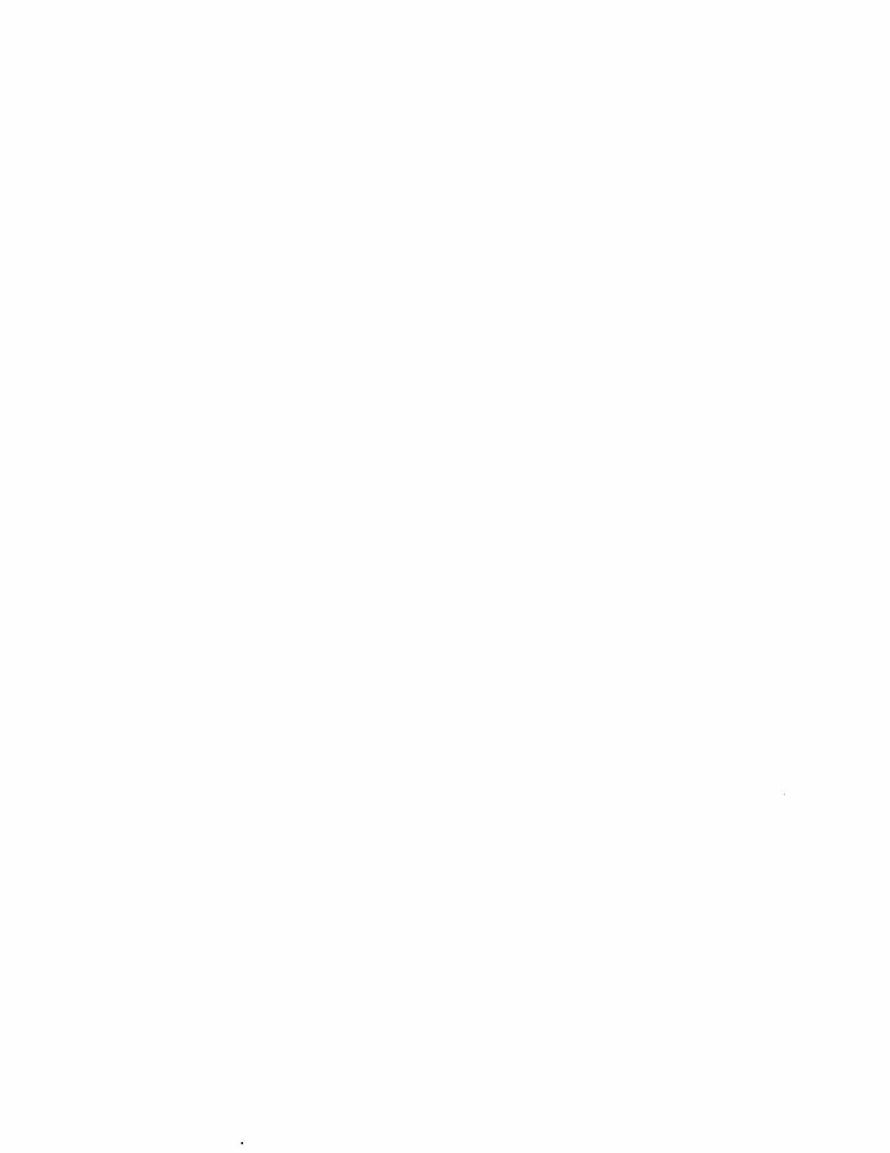
List Of Figures

Figure

1.1 (1,3) Constraint Graph 3

1.2 (2,00) Constraint Graph 6

1.3 Diagram of Rectangular Wave Form 7

1.4 (1,3)£ = 5 Level Charge Constraint Graph 10

1.5 (0,1)£ = 2 Level Charge Constraint Graph 18

1.6 Paths of Length Two Graph 18

1.7 (0,3)£ = 4 Level Charge Constraint Graph 20

1.8 Paths of Length Two Graph 21

1.9 Reduced Paths of Length Two Graph 22

1.10 Coding Scheme Using H Code , 26

2.1 Covering Space of (0,00) Constraint Graph 45

2.2 Covering Space of (1,3) Constraint Graph '" .. 45

2.3 Split Figure GK 57

2.4 Four Fold Covering of (1,3) Constraint Graph 59

3.1 Conventional Coding Scheme , , G2

3.2 Three Fold Covering of (1,2) Constraint Graph G7

3.3 Eight Fold Covering of (0,2) Constraint Graph 69

3.4 Eight Fold Covering of (0,00) Constraint Graph 71

viii

3.5 Shift Register for Dividing by g(x) 75

3.6 Error Check Covering for (1,3) Constraint Graph 86

A.1 Algorithm for Finding dfr ee of a Ternary Convolutional Code 100

ix

Chapter 1

Capacity for the (d, k) Constrained Codes

1.1 INTRODUCTION

In this chapter, the capacity of the (d, k) constrained codes is discussed. We de­

rive an equation for the capacity of the (d, k) L level charge constrained codes. The

case of rational capacity is considered and we point out an errol' in the literature.

This leads to an interesting new code for the (0.3) L = 4 level chargc constraints.

The last part of the chapter deals with possible implementations for this code,

1.2 CAPACITY

A (d, k) constrained sequence is a binary sequence in which two consecutive ones

are separated by at least d zeros and at most I.: zeros.

A (d, k) constrained code is a mapping of binary sequences to thc set of (d, h:) con­

strained sequences. These codes are also refercd to in the literature as run-length

limited codes. They have attracted much recent interest as they are important for

magnetic and optical recording. The paper of Siegel provides a good introduction

to the (d, k) constrained codes. Other references arc given in the bibliography.

Shannon showed that there is an upper bound for the rate of a constrained code.

This bound is called the capacity of the code. In the literature, the term capacity

has been used with some ambiguity. In [ZW], the capacity of the (d, h:) constrained

codes is found, in [8] and [TB], the capacity of the channel is found when using a

(d, k) constrained code, and in [AS], the capacity of the (d, h:) constrained systems

is found. In each instance, they are talking about the same thing. We will use the

description "capacity of the (d, k) constrained codes" in this paper.

. . . . log N(TI,)From Shannon, we see the capacity IS given by c = lim where N (n)

n-oo 'II,

is the number of constrained sequences of length u, If the base of the logarithm is

taken to be b. then we say that c is the base b capacity of the constrained code.

The capacity of the (d, k) constrained codes has been derived several times in

the literature. In [TB], the capacity of the (d. k) constrained codes is found by

counting the number of constrained sequences. In [ZW], the capacity is found

using a probabilistic approach. And in [ACH] it is found using the state transition

matrix of the (d. k) constraint graph. We follow the later approach to rederive the

capacity of the (d, k) constrained codes.

Associated with the (d, k) constrained sequences is a id; k) constraint graph.

Thc (d, h;) constraint graph has h: + 1 vertices and 2k - d + 1 edges. Labeling the

vertices ai, 1 :::; .; :::; l: + 1, we get that the edges arc:

(1) for 1 :::; i :::; k,

for d + 1 :::; i :::; k + 1,

The edges of the graph that enter vertex (1,1 are labeled with a one. All other edges

are labeled with zero. For example, the (1,3) constraint graph is shown below. The

2

study of the (d, 1.:) constrained sequences using thc associated constraint graph was

introduced by Shannon.

o o o

Figure 1.1: (1,3) Constraint Graph

Let T be the state transition matrix for a (d, Ii,) constraint graph. The entry

tij is one if there is an edge in the graph from the i t h vertex to the ph vertex.

Otherwise the entry is zero. The state transition matrix is a square matrix whose

entries are nonnegative. For example, the state transition matrix for the (L 3)

constraint graph is shown below.

(2)(

0 1 0 0 )T= 1010

100 1

100 °Wc digress now to the Perron-Frobenius theory of nonnegative matrices. The

necessary facts can be found in [V].

A nonnegative square matrix T is irreducible if for all i and i. there is a positive

intcger n such that t~j) > 0 where tg1) is the ilh entry of T": The state transition

matrix for a (d, l.:) constraint graph is an irreducible matrix.

3

The Perron-Frobenius theorem for nonnegative matrices, as found III [V]. IS

shown below.

Theorem 1. (Perron-Frobenius). Let T be an irreducible nouuegetive square

matrix. Tlwll

1. T has a positive real eigeuvslue A. witl: A ~ I//,I for all oilier

eigeuvelucs Il ofT.

2. To A there corresponds an eigenvector '(/I whose entries arc positive reels.

3. A is a simple eigenvalue ofT.

The dominant real eigenvalue will be referred to as the Perron eigenvalue.

The base b capacity of the (d, h~) constrained codes, according to Shannon, is

equal to Iog, A where A is the Perron eigenvalue of the state transition matrix for

the (d, k) constraint graph.

We rederivc the capacity for the (d, k) constrained codes starting from the eigen­

vector equation Tic = AW. We call the entry ui; of the eigenvector, the weight of

the state i. The eigenvector equation then says that the sum of the weights of the

successors for a state will equal A times the weight of the state. Or alternatively,

A-1 times the weight of the successors is equal to the weight of the state.

Starting from the first vertex of the id: k) constraint graph, and following all

possible paths until they return to the first vertex gives the equation:

(3)

4

From the Perron-Frobenius theorem. we know that 'WI IS nonzero. Dividing by

'lUI and rearranging gives the equation:

(4)

The Perron eigenvalue is the largest real solution of this equation and the capacity

of the id, k) constrained codes is the logarithm of this eigenvalue.

The same expression for the capacity of the (d. k) constrained codes has appeared

many times in the literature. for instance [ACH], [TB]. [AS], and [NB].

If no k constraint is imposed, we get the (d. 00) constraints. A binary sequence

satisfies the (d, 00) constraints if two consecutive ones are separated by at least

d zeros. No limit is imposed on the number of consecutive zeros. According to

Shannon, the capacity for the (d, 00) constrained codes can be calculated in the

same way as above for the (d, k) constrained codes. We start with the (d, 00)

constraint graph and use the eigenvector equation for the state transition matrix

to find the Perron eigenvalue of the state transition matrix. The (d, 00) constraint

graph has d+ 1 vertices and d + 2 edges. If we index the vertices from one to d +1,

the the edges will be:

(5) for 1 ~ 'i ~ d,

for z = d + 1,

5

The edge in the graph that enters vertex a1 is labeled with a one. All other

edges are labeled with zero. As an example of the (d, 00) constraint graph. the

(2,00) constraint graph is shown below.

o

Figure 1.2: (2,00) Constraint Graph

To solve the eigenvector equation, we use the fact that the weight of a state is

equal to A-1 times the weight of its successors. Starting from the last state of the

(d, 00) constraint graph, this becomes 'lVd+1 = A -lw,H1 + >. -(d+l)Wd+1' Rearrang­

ing gives the equation A d+1 - Ad - 1 = O. The capacity of the (d, 00) constrained

code is equal to the logarithm of the largest real solution of the equation. This has

appeared before in [ACH] and [TB].

We note here that the capacity of the (d, 00) constrained codes is larger than

the capacity of any (d, k) constrained code for the same d. This follows as there

are more sequences if no k constraint is imposed than if there is a k constraint

imposed. We will use this fact later in the next section.

6

1.3 (d, k)L LEVEL CHARGE CONSTRAINED CODES

An important subclass of the (d. I.:) constraintcd codes is the (d. k) charge con­

strained codes. These codes have been previously considered in [AS] and [ NB].

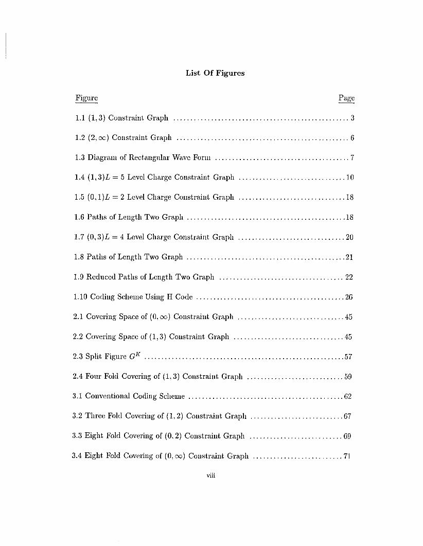
To motivate the definition of a charge constrained sequence. consider a (d, k)

constrained sequence v. Associated with v is a rectangular wave form l,,(t) which

represents the current when transmitting the sequence '/1. The ones in u represent

the transitions of Iv(t) and the zeros represent no transition. A diagram of this

process is shown below. The clock is assumed to tick at integer intervals and the

transitions to occur at times I.~ + ~, k E Z.

info

clock

o 0 000 0 o 0 0 0 o 0 o 0

-I~-I I tFigure 1.3: Diagram of Rectangular Wave Forni

The charge that a capacitor accumulates from the wave form Iv(t) is given by

J2 l,,(t)dt. It is very desirable for the accumulated charge to be bounded. As

7

noted in [AS], the accumulated charge being bounded ensures that the code has a

spectral null at de.

A (d, k) constrained sequence satisfies the L level charge constraint if there is a

nonnegative integcr 7 ~ L such that for all to. t1 , the accumulated charge satisfies:

(6)

A (d, k) constrained code is said to be a (d, k)L level charge constrained code if

there is a nonnegative integer 7 ~ L such that all code sequences satisfy the L level

charge constraint for the integer 7.

We can calculate the charge accumulation for a (d, A:) constrained sequence by

calculating its running digital sum. This is noted in [AS]. To understand the

running digital SUIll, consider v a (d, k) constrained sequence. Parse 'U into blocks

of length between d + 1 and k + 1, each block ending in a one. Let b, be the number

of zeros in the i t h block of the parsed sequence. The running digital sum for the

sequence 'U is then I:~~I(-I)ib'i' This is useful. as for the rectangular wave form

in the first ti blocks of the parsed sequence. Thus, an equivalent condition for a

sequence to satisfy the L level charge constraint is for its running digital sum to

be bounded between -7 and L +d - 7.

We want to derive an equation for the capacity of the (d, k)L level charge con-

strained codes. Wc usc a directed graph for the (d. k) L level charge constrained

8

codes, and follow the method used ill the previous section for finding the capacity

of the (d, k) constrained codes.

The (d, It;)L level charge constraint graph will consist of vertices labeled with a

double index i and j. The index i corresponds to the state the sequence would be

in for the (d, It;) constraint graph, and the j corresponds to the charge level. The

indices are required to satisfy 1 ::; -£ ::; It; + 1, 1 ::; j ::; L + a, and 0 ::; .i - i < L.

The edges for the graph are then:

(7) for 1 ::; i <k;

for d + 1 ::; i ::; It; + 1

(Li.j ---t (Li+l,j+l

The edges of the graph that enter a state whose i index is one are labeled with a

one. All other edges are labeled with a zero. As an example, the (1, 3)L = 5 level

charge constraint graph is shown below.

1 • to aj 1

6 6 6,

6

to a 1 2,

5

to a 1 3,

4

jto a 1 4index ,

3

to al 5,

24

3

2 iindex

Figure 1.4: (1, 3)L = 5 Level Charge Constraint Graph

10

It is clear that a sequence generated from the (d, k)L level charge constraint

graph, which starts in vertex eLi). will have its running digital sum bounded between

- j and L + d - j. Thus, the sequence will be a (d, k)L level charge constrained

sequence.

The capacity of the (d, 1.~)L level charge constrained codes, as it was for the

(d, k) constrained codes, will be the logarithm of the Perron eigenvalue for the

state transition matrix of the constraint graph. An equation for the capacity of

the (d, k)L level charge constrained codes when L + d is even is derived in [NB].

We derive a similar equation for the (d, 1.~)L level charge constrained codes.

To find the Perron eigenvalue, we start with the eigenvector equation Tio = Xu).

This says that the weight of a state is equal to >.. -1 times the weight of its successors.

Using the L states whose i index is one, we get the set of L equations shown below.

Only the j index is used to denote the weight of the state 'WI,j:

'WI = >..-Cd+I)'WL +>..-(tl+2)WL_I + +>..-C!.:+I)'WL+d_k

'W2 = >.. -Cd+I)'WL_I + >.. -(d+2)'WL_2 + + >.. -Ck+I)'WL+d_k_I

(8)

'WL-I = >..-Cd+I)W2 + >..-C'J+2)WI

'WL = >..-Cd+I)WI

Writing these as a matrix equation gives 'Ill = A,\'llI, or (A,\ - I)'IlI = O. For this

to occur, the determinant of A,\ - I must equal zero. We state this as a theorem.

11

Theorem 2. The capacity of the (d, k)L level charge constrained codes will be

equal to the logarithm of the largest real solution of the equation detA = O. where

tile matrix A has its iph enity es A-(i+j+l-L) f(i +j + 1 - L) - 6ij witu (iij the

{I for d + 1 < p < k + 1

Kroetiicket delta function and f (p) = . - - .ootherwise

To illustrate the theorem, we work out as an example the capacity for the

(1, 3)L = 5 level charge constrained codes. The constraint graph for the (1, 3)L = 5

level charge constraints is shown above. Using the five vertices whose i index is

one and the fact that the weight of a state is equal to A-I times the weight of its

successors, we get the five equations shown below:

(9)

\ -2W5 = /\ WI

Combining these into a matrix equation, we get the equation (AA - I)w = O.

This equation has a solution only when det( AA - 1) = O. This equation is shown

below:

-1 0 A-4 A-3 A-2

0 A-4 -1 A-3 A-2 0(10) det >.-4 A-3 >. -2 _ 1 0 0 =0

A-3 x-2 0 -1 0>.-2 0 0 0 -1

12

Working out the determinant gives us the equation (1-2>, -2)(1 +). -2 )(1-), -4) =

O. The largest real solution of this is clearly..j2. The binary capacity for the

(1, 3)L = 5 level charge constrained codes is then c = log2 12= ~.

We point out that for the cases where L +d is even, the equation for the Perron

eigenvalue in [NB] reduces to the same equation as in the theorem.

1.4 RATIONAL CAPACITY

We want to determine which (d, k)L level charge constrained codes have ration­

al capacity. This was considered in [AS], where the codes with L + d even are

examined. We extend their results to all the (d,k)L level charge constrained codes

and point out an error in a statement of theirs. The development of this section

follows that of [AS].

The key to determining if the (d, l.:)L level charge constrained code has rational

capacity is the relationship between the capacity of the constrained codc and the

period of the constraint graph. The period of a graph is equal to the greatest

common divisor of the lengths of all the loops in the graph. We first determine the

period of the (d, k)L level charge constraint graphs.

Lemma 3. TIle period of tlie (d, h:)L level cluitge constraint gtnpl: divides two.

])7'001. Starting from the vertex all, the path determined by the sequence of d zeros

followed by a one, repeated twice, will he a loop in the graph.

13

Similarly, the sequence of d +1 zeros followed by a one. repeated twice. will be

a loop in the graph.

Since the period of the graph divides the length of each loop, we see that the

period must divide 2(d + 1) and 2(d + 2). This occurs only if the period divides

two. 0

Theorem 4. The (d, k)L level charge constraint gtepl: has period one if L + d is

odd.

J)1·OO/. Suppose L + d is odd. We will show that there is a loop in the constraint

graph of odd length.

If L is odd, then consider the path in the graph starting from vertex a1,[.[;.J+1

and determined by the binary sequence of d zeros followed by a one. The path

will be in vertex ad+l,[1tJ+d+1 after the d zeros. The one will send the path to the

vertex a1,m where m. = L + d + 1 - ([~] + d -I- 1) = L - [tJ = [~J + 1. Thus the

path is a loop in the graph and its length is tl + 1. The period of the graph must

divide the length of any loop, so the period will divide d + 1. Since L is odd and

L + d is odd, d + 1 will be odd. The lemma says that the period divides two, and

we have shown that the period divides an odd number. Thus the period is one.

If L is even, then consider the path in the graph starting from the vertex a 1,-{t

and determined by the binary sequence of d + 1 zeros followed by a one. The path

will be in vertex ad+ 2,d+I+1t after the zeros and in vertex rLl,m after the one, where

14

ni = L + d + 1 - (d + 1 + t) = t. Thus the path is a loop in the graph of length

d + 2. Since L + d is odd and L is even, d +2 is odd. Thus by the same reasoning

as above, the period of the graph is one. 0

Theorem 5. TIle (d, k)L level cluuge coustteitit graph has period two i[ L +d is

even.

]JTOOf. Suppose that L + d is even. We show that all loops have even length.

Let Va be the set of vertices in the graph whose j index is even, and let VI be

the set of vertices whose j index is odd. An edge in the graph connects two vertices

in opposite sets. A path in the graph which starts from a vertex in Va will end in a

vertex from VI if the path is odd length. Similarly, a path which starts in a vertex

in VI will end in vertex from Va if the path is odd length. Thus, any loop must be

of even length.

The lemma showed that the period divides two and we have shown that all loops

have even length. Therefore, the period for the graph is two. 0

We digress again for a moment to the Perrou-Frobenius theory for nonnegative

matrices. The necessary facts are found in Varga. We condense them into the

following theorem.

Theorem 6. TIle state trensition matrix [or a grepl: whose period is p will luivo

''2rrl

p eigetivelues oi maximum modulus. Tuese eigeuvelues will be of the form AC I P .

[or 0 ::; l ::; p - 1, wuete A is tlie Perron eigeuvelue oi the stnie tteusitiou matrix.

15

We use this theorem to show the possible rational capacities for the (rl, I.:) L level

charge constrained codes. The key lemma from Ashley-Siegel shows how the period

of the constraint graph is related to the capacity of the constrained codes.

Lemma 7. (Ashley-Siegel). If tile (d, k)L level cluuge cousireiued code lies

rational cepecity' f for any base b. tiicu tlie period of tlie (d, k)L level clutrge gtepl:

is a multiple of s.

P1'Oof. Since c = ~, the Perron eigenvalue of the state transition matrix T will be

b~, where b is the base of the capacity. This eigenvalue is a root of the polynomial

m,(x) = x" - v, which is. irreducible. So Tn(x) must divide the characteristic

polynomial of T. Thus, the roots of m(x) are eigenvalues for T. where the roots

t '21:'1are b. e1

· - s for 0 ::; l ::; s - 1.

Theorem six shows that for a constraint graph with period p, there are p eigen-

values of maximum modulus for the state transition matrix T. These eigenvalues

'27d

being of the form >.e1p-, for 0 ::; l ::; p - 1.

Equating these two facts, we sec that for some lo,

only if fa = s, thus showing the lemma. 0

i 2rr/Qe p This occurs

We combine this lemma with the theorems for the period of the (d, k)L level

charge constraint graphs to show which rational capacities arc possible.

Theorem 8. TIle only possible tetiousl capacities for tlu: (d. k)L level chnige

constrained codes are bituuy tete 1/2 and tC1'11alY rate 1/2 wIlen L + d iH even.

16

proo]. If L +d is odd, the period of the (d, k)L level charge constraint graph is one,

So by the lemma, the only possible rational capacities arc of the form 'In/I. Since

this is greater than one, and the capacity of a constrained code is less than one,

we see that no such codes with rational capacity can exist,

If L + d is even, the period of the (d, k)L level charge constraint graph is two.

So by the lemma, the possible rational capacities are of the form '117,/2. Only the

case with 111 = 1 will give a capacity less than one.

If the base b capacity were 1/2, then the binary capacity will be log2 b~. Only

the cases for b = 2 and b = 3 will have binary capacities less than one, 0

We work some examples of (d, k)L level charge constrained codes which have

rational capacity.

The first case we consider is for the (0, l)L = 2 level charge constraints. The

equation for determining the capacity of the (0, l)L = 2 level charge constrained

codes is found from theorem two to be:

(11)1

,,\ - 2 -1det ,,\-1

,,\-1 I=0-1

The determinant in the equation reduces to 1 - 2), -2 which has largest real root

equal to J2. The binary capacity is then equal to log2 J2= 1/2.

To get a (0, l)L = 2 level charge constrained code, we examine the (0, l)L = 2

level charge constraint graph. The constraint graph and the graph of paths of

length two are shown below.

17

Figure 1.5: (0, l)L = 2 Level Charge Constraint Graph

al,2 10 a2,2

11~....~__-~ 1011

Figure 1.6: Paths of Length Two Graph

We can design an encoder by choosing a connected component of the paths of

length two graph. Taking the component consisting of the single vertex, we get

an encoder by labeling the 01 edge with 0 and labeling the 11 edge with 1. The

encoding/decoding table for this code arc shown below.

18

Table 1.1: Encoding Table for (0,1) Constrained Code

input outputbit block

o1

0111

This code is called frequency modulation or phase encoding. As noted by [AS],

it was an early standard in magnetic recording.

As a second example, we consider the (1. 3)L = 5 level charge constrained codes.

As we showed earlier, the (1, 3)L = 5levcl charge constrained codes will have binary

capacity rate 1/2. Unfortunately, the method for designing an encoder used for the

first example does not work for the (1,3)L = 5 level charge constraints. In fact,

there does not appear to be a simple way to encode for these constraints at rate

1/2.

As a final example, we consider the (0. 3)L = 4 level charge constrained codes.

The equation for determining the capacity of the (0,3)L = 4 level charge con-

strained codes is found from theorem two to be:

(12) det =0

The determinant in the equation reduces to (1 - 3>' -2)(1 + >. -2), which has

largest real root equal to J3. The ternary capacity of the (0. 3)L = 4 level charge

constrained codes is equal to log3 /3 = ~.

10

The method used ill the first example does work for the(O. 3)£ = 4 level charge

constrained codes to give an encoder. We start with the (0,3)£ = 4 level charge

constraint graph and look at the graph of paths of length two. The constraint

graph and the paths of length two graph are shown below.

_--__--_---__~~ to all,

jindex

4

3

2

2

3

iindex

'----a~ to a 1 2,4

to a 1 3,

to a 1 4,

Figure 1.7: (0,3)£ = 4 Level Charge Constraint Graph

20

11

Figure 1.8: Paths of Length Two Graph

Now notice that the vertices a2.3 and a3,3 have the same successors in the graph

of paths of length two. Also note that each has the same binary pattern for the

edges with the same terminal vertex. So, we merge the two vertices together. This

gives the reduced paths of length two graph shown below.

21

11 a 100C ,_3_1O ~~_

'0-

Figure 1.9: R.educed Paths of Length Two Graph

This graph has three edges outgoing from each vertex and three edges incoming

to each vertex. By using the ternary field GF(3) we can design all encoder from

the reduced graph. The encoder will be obtained by labeling the 01 edges with

1, labeling the 11 edges with 2, and labeling the 00 and 10 edges with O. The

resulting encoding tables are shown below. We will call this (0,3)L = 4 level

charge constrained code the H code.

Table 1.2: Next State Table for H Code

illput trit

0 1 2present all x 0,13 all

state a13 x all (£13

x ;c all 0,13

22

Table 1.3: Output Table for H Code

input trit

present

state

o001010

1010101

2111111

By the choice of the labels, the decoder will be independent of tho state that the

sequence is in. This property will ensure that errors induced by the channel will

not be propagated by the decoder. This is a very desirable property for practical

applications. The decoder table for the code is shown below:

Table 1.4: Decoding Table for H Code

Input TernaryOutput

00011011

o1o2

In the final section of this chapter, we will examine possible applications of the

H code.

We note that the (0,3) charge constrained codes have been previously considered

in the literature. The article of Patel describes a (0.3) charge constrained code

constructed in a manner different from the H code. The code of Patel turns out to

be a (0,3)£ = 10 level charge constrained code.

23

These three codes are the only id, J.:)L level charge constrained codes which have

rational capacity for any base. This generalizes the main result from Ashley-Siegel.

Theorem 9. TIle only (d, k)L level cllarge constrained codes whicll luive tniiounl

capacity are tlie (0, l)L = 2 and tue (1, 3)L = 5 level charge constrained codes

at biuery capacity rete 1/2 end the (0, 3)L = 4 level cluugc coustmiued code at

tenuuy rate 1/2.

proof. The examples above show that each code has the capacity claimed by the

theorem.

Recall that the capacity of the (d, (0) constrained codes will always be larger

than the capacity of any (d, k)L level charge constrained code with the same d. We

use this to show that no other (d, k)L level charge constrained codes with rational

capacity exist.

First consider the capacity of the (1, (0) constrained codes. The polynomial

for the Perron eigenvalue of the (1, (0) constraint graph state transition matrix

is >. 2 - >. - 1. It is easily checked that the largest real root of this polynomial is

less than J3. This implies that no (d, k)L level charge constrained code for d 2: 1

can have ternary capacity rate 1/2. The case where d = 0 gives the (0,3)L = 4

level charge constrained code shown above. This shows that no other td, I.:)L level

charge constrained codes exist with ternary capacity rate 1/2.

24

Now consider the capacity of the (3, x) constrained codes, The polynomial

for the Perron eigenvalue of the (3, 00) constraint graph state transition matrix is

>.4 - >.3 - 1. It is easily checked that the largest real root of this polynomial is

less than J2, This implies that no (d, k)L level charge constrained code for d ~ 3

can have binary capacity rate 1/2. The cases where d = 0 and d = 1 give the

(0, I)L = 2 and the (1, 3)L = 5 level charge constrained codes mentioned above.

The case where d = 2 must be considered separately. If L is odd. then by the

theorem eight there will be no (2, k)L level charge constrained code with rational

capacity. If L is even, then by examining the table from [NB], we sec that no

(2,k)L level charge constrained code with binary capacity rate 1/2 exists. 0

This completes showing all the (d, I.;) L level charge constrained codes which have

rational capacity. In [AS], they consider the td, k)L level charge constrained codes

for which L + d is even. They use the notation .,(d. k; c) charge constrained system"

to represent what we are calling the (d, k)L = 2c - d level charge constrained code.

The theorem corrects a statement in the article [AS], where it is claimed that

"the only (d, k; c) charge constrained systems with rational base b capacity are

the (0,1; 1) and (1,3; 3) charge constrained systems where the base is a power of

two." The additional code for the (0,3)£ = 4 level charge constraints corrects their

statement.

25

1.5 A (0,3)L = 4 LEVEL CHARGE CONSTRAINED CODING SCHEME

We examine possible applications using the H code. The encoding and decoding

tables for this code were shown above. The encoder takes a ternary sequence and

outputs a binary sequence that satisfies the (0, 3)L = 4 level charge constraints. In

typical applications, the information to be encoded is binary, not ternary. Thus to

use the H code, we must first convert the binary sequence into a ternary sequence.

Then the H code can be implemented to give a binary (0,3)L = 4 level charge

constrained sequence. A coding scheme for this process is shown below.

ErrorH Code- b i tI tr it - ControI -- conver t ..

Code - Encoder

, w

channe 1

bi tI tr i t ECC H Code~ - - -inver t - Decoder -- Decoder --

Figure 1.10: Coding Scheme Using H Code

Notice that the error-control code can be put between the bit-trit converter and

the H code encoder. The error-control code will be a code using the ternary field

GF(3). Recall that we earlier showed that the H code does not propagate errors.

26

Thus, errors in the channel will reach the error-control code without effecting the

adjacent trits in the ternary sequence. This is a very desirable property.

First we consider the bit-trit converter. We want an arbitrary binary sequence

to have a representation as a ternary sequence. This will be possible at a rate of

piq as long as there are more binary sequences of length p than there are ternary

sequences oflength q. The limiting rate, as we prove below, for the bit-trit converter

will be log2 3.

Lemma 10. A rate plq bit-ttit converter exists for all rl« less tlieu log2 3.

]J1'Oof. If piq ~ log23, then 2P ~ 3Q• This says that there are more ternary sc-

quences of length q than there are binary sequences of length p. This is exactly

what is needed for there to be a bit-trit converter of rate E. 0Q

So, the limiting rate for a bit-trit converter will be log2 3 = 1.58496. For practical

purposes, it is necessary to keep p and q small. Consider if we use a bit-trit converter

that converts binary sequences of length p into ternary sequences of length q. If

an uncorrected error occurs in the ternary sequence, then this error will affect the

entire length p binary sequence. Thus the p represents the length an uncorrected

error can propagate in the output sequence.

27

Possibilities for the bit-trit converter with small p and 'l are:

Table 1.5: Possible Bit/Trit Converters

plq p q3/2 = 1.5 3 2

11/7 = 1.57 11 719/12 = 1.58 19 12

We now consider possible ternary error-control codes. There are two well de-

veloped types of error-control codes, block codes and convolutional codes. We

examine the possibilities for both types of codes.

A block code partitions the information sequence into blocks of length k, Each

block is encoded independently into a block of length n. See [SM], [LC]. or [PW]

for an introduction to block codes.

The rate using the coding scheme will always be less than the capacity of the

(0,3)L = 4 level charge constrained code, which in binary terms is log2 J3 = .7925.

Suppose that in the coding scheme. we use a rate ~ bit-trit converter and a rate

s. block code. For pk input bits, the bit-trit converter outputs qk trits. The ternaryn

error-control code takes the qk trits, and outputs qn. trits, The H code encoder

takes the qn trits, and sends 2qn bits to the channel. The rate of the coding scheme

pkis then --.

2qn

For comparison. we present the rate for the coding scheme using various cornbi-

nations of bit-trit converters and ternary block codes. The rates were found using

the formula above.

28

Table 1.6: Possible Coding Rates Using Block Codes

Ternary Block Code Bit/Trit Converter Rate

Golay [11,6,5]

Hamming [26,23,3]

3/2 .40911/7 .428

19/12 .431

3/2 .66311/7 .695

19/12 .700

The other type of commonly used error-control codes are the convolutional codes.

Convolutional codes are popular because simple encoding and decoding techniques

exist. A rate s. convolutional code partitions the input sequence into blocks of11.

length k and outputs a block of length 17" formed as a linear combination of the

input block and the m previous input blocks. For an introduction to convolutional

codes, see [LC] or [PW].

There docs not appear to have been any published list of ternary convolutional

codes in the literature. This can be explained since most practical situations use

binary codes. For possible applications of the H code. it desirable to have a table of

ternary convolutional codes. The table below shows the rate 1/2 noncatastrophic

ternary convolutional codes of largest free distance. These codes were found using

a computer search that implements a modified version of the algorithm in [L]. In

the appendix, the algorithm is discussed.

29

Table 1.7: Rate 1/2 Ternary Convolutional Codes With Largest dfree

memory 91 92 dfrcc

2345678

(1,2,2) (1,1,1) G(1,1,1,2) (1.0,1.1) 7

(1,1.1,2,1) (1,0,2,1,1) 9(1,0,1,2,2,1) (1,0,1,1,2,2,) 10

(1,1,1,0,2,1,1) (1,0,2,1,2,2,1) 12(1,0,2,1,1,0,2,2) (1,0,1,2,1,1,1,2) 13

(1,1,0,2,2,1,1,1,2) (1,0,2,1,2,0,2,1,1) 15

Suppose that in the coding scheme, we use a rate ~ bit-trit converter and a rate

1/2 ternary convolutional code. For p input bits, the bit-trit converter outputs q

trits. The ternary convolutional code takes the q trits and outputs 2q trits. The

H code takes the 2q trits, and sends 4q bits to the channel. The rate of the coding

scheme using a rate ~ bit-trit converter and <L rate 1/2 ternary convolutional code

is then ;fq.

Possible rates for the coding scheme using a rate E bit-trit converter and a rateq

1/2 ternary convolutional code are presented in the table below:

Table 1.8: Coding Rates When Using Rate 1/2 Ternary Convolutional Code

Bit/Trit Converter Rate of Coding Scheme

3/211/7

19/12

30

.375

.392

.395

1.6 CONCLUSION

In this chapter, we have introduced the (d. k) constrained codes and the (d, k)L

level charge constrained codes. An equation is derived to compute the capacity of

the (d, k)L level charge constrained codes. It is shown that the only (d, k)L level

charge constrained codes with rational capacity arc the (0, l)L = 2 and (1, 3)L = 5

level charge constrained codes at binary capacity rate ~ and the (0,3)L = 4 level

charge constrained code at ternary capacity rate ~. The last section of the chapter

examines possible applications of the (0.3)L = 4 level charge constrained code.

31

Chapter 2

Topological Properties of

the (d, k) Constraint Graphs

2.1 INTRODUCTION

In this chapter, we discuss the topological properties of the (d, k) constraint

graphs. The chapter is intended as an introduction, for the nonexpert, to some

basic topological facts. In the first section, the fundamental group is defined. In

the second section, a covering space is defined and some basic properties of covering

spaces are examined. In the last section of the chapter, a constructive proof is given

for building a covering space for a (d, k) constraint graph.

2.2 THE FUNDAMENTAL GROUP OF A (d, k) CONSTRAINT GRAPH

The (d, k) constraint graph has k + 1 vertices and 2k - d + 1 edges. Labeling

the vertices, ai, 1 ~ i ~ k: + 1, the edges are:

for 1 ~ i ~ k,

(1)for d + 1 ~ i ~ k +1, ai -t al

The edges in the graph that enter vertex al are labeled with a one. All other

edges are labeled with zero. The (d, k) constraint graphs were introduced in the

previous chapter.

32

We also want to consider the (d. (0) constraint graphs. The (d.x) constraint

graph has d + 1 vertices and d + 2 edges. Labeling the vertices tu, 1 :s; i S d + 1.

the edges are:

(2)for i = d + 1, a'1+I --t al and ad+1

The edge in the graph that enters vertex al is labeled with a onc. All other

edges are labeled with zero. The (d, (0) constraint graphs were introduced in the

previous chapter.

We will use the term "constraint graph" to mean a (d, k) constraint graph or a

(d, (0) constraint graph. We will work only with constraint graphs ill this chapter,

but we note that the development works for finite graphs.

For an edge in a constraint graph, we use c- I to represent the reversed edge of

the edge e. That is, if e is an edge from vertex c; to vertex aj, then the reversed

edge is the edge from vertex aj to vertex a; obtained by reversing the direction of

the edge e. We call e a proper edge and e- I a reversed edge.

An edge path in a constraint graph is a sequence of edges, P = (PI, P2 . . . . •Pn),

where each Pi is a proper edge or a reversed edge in the constraint graph G. and

for each i, the terminal vertex of Pi is the initial vertex of PHI. Ifrz is the initial

vertex of PI and u is the terminal vertex of pn, then we say P is an eclge path from

'/1, to v. An edge path from a vertex '/1, to itself will be called a loop at the vertex u.

33

A reduced edge path will be an edge path such that for each i, the edge Pi is

not the reversed edge of the edge Pi+I. An edge path p = (PI ~ P2, ...• Pn) which is

not a reduced edge path has an associated reduced edge path. If Pi is the reversed

edge of the edge Pi+I, then a reduction of P can be done by removing the edges Pi

and Pi+I from the edge path. This reduction process is repeated on the resulting

edge path until a reduced edge path is reached. The edge path obtained will be

called the reduced edge path associated with the edge path p. We note that the

reduced edge path associated with an edge path is unique.

If each edge Pi from the edge path P is a propel' edge from the constraint graph.

then we say that P is a proper edge path for the constraint graph. For a proper

edge path P = (PI, P2, ... , Pn), there is an associated (d, k) constrained sequence

s = (SI' S2, ... , 8n ), where Si is the binary label of the edge Pi in the constraint

graph. In the next chapter, we will construct (d. k) constrained codes using the set

of proper edge paths for the (d, k) constraint graph. Note that a proper edge path

for a constraint graph will be a reduced edge path.

The length of an edge path P = (PI, P2, ... , (In) will be the number of edges in

the edge path. For instance, the length of P is n.

Let 'U be a vertex from the constraint graph G. Let W u be the set of all finite

length reduced edge paths which are loops at the vertex 'U. We define a product

on W u which makes W u into a group.

34

Suppose P = (PI,P2, ... ,Pn) and T = (TI,T2, ... ,Trn) are clements of W/L' To

define the product pr, we find the smallest integer i such that the cdge Ti is

not the reversed edge of the edge (Ju+I-i. The product (JT is then defined to

be (PI, ... , Pn+I-i, Ti, .. . ,Tm). It can be verified that the product pr is a reduced

edge path which is a loop at u, Thus pr is an element of W'/L' To show that Wu is

a group with this product, we have to show that there is an identity clement and

that for each P in W/L' there is an inverse element p-I in W'/L'

Consider the empty sequence. This represents the loop at 'IL which never leaves

the vertex 'U. We use 1 to represent the empty sequence. It is easily verified that

1 is an identity for the set W/L with the product defined.

For an element P = (PI.P2, ... ,Pn), consider the element p-I = (p;;I"",PI I),

where pi! is the reversed edge of the edge Pi. The product of P and p- I will then

be equal to empty sequence L showing that p- I is an inverse for p in W/l'

The edge paths (pT)O' and p(7(J) will both be equal to the reduced edge path

associated with the edge path obtained by concatenating Tonto p and then con­

catenating 0' onto the resulting edge path. Since the reduced edge path is unique,

the associative property holds.

This suffices to show that W/L is a group with the product defined. This group

IS called the fundamental group of the constraint graph at the vertex '/1,. The

fundamental group of the constraint graph at the vertex u. will be denoted as

7r( G, 'U). The fundamental group of a space is well known ill topology. For an

35

introduction to the fundamental group presented in greater generality, the reader

is referred to [M] or [GH].

We want to show that the fundamental group of a constraint graph is a free

group. It is a well known fact that the fundamental group of any graph is a free

group. See [M] for a proof of this. We rederive the fundamental group of a (d, k)

constraint graph. The development of this section follows that in [M].

We start out by determining what a maximal tree for a constraint graph is. A

tree is a connected graph with one more vertex than edge. A maximal tree for a

constraint graph is a subgraph which is a tree and is contained in no other subgraph

that is a tree. It turns out to be easy to determine if a tree is a maximal tree for

a constraint graph.

Theorem 1. Let G be a constraint graph and let t a subgtnpl) of G wliicl: is a

tree. Then t is a maximal tree for G if and only if t contains all t11C vertices of G.

]JTOOf. If t contains all the vertices of G. then any additional edge would connect

two vertices of t. Thus the additional edge would give a graph which is not a tree.

So, the subgraph t is a maximal tree for G.

If t does not contain a vcrtcxv in G, then let P be the set of edge paths in G

that connect a vertex of t to the vertex u. Since G is connected, we know that P

is a uonempty set. Let p be the edge path in P of shortest length. Let X be the

subgraph of G whose edges are the edges from the edge path p, It is easily verified

36

that the subgraph X U t will be a tree which contains t. Thus t is contained in

another subgraph which is a tree. So t is not a maximal tree for G. This completes

the proof of the theorem. 0

There are typically several different maximal trees for a constraint graph. The

maximal trees for the (1,3) constraint graph and for the (2, (0) constraint graph

are shown below as examples:

Table 2.1: Maximal Trees for the (1,3) Constraint Graph

tl ={a1 a2,(L2(L3,a3 a4}

t2 ={ (L1a2, (L2(L3, a4(L1}

t3 ={(L1a2,a3(L4,a4ad

t 4 ={ 0,20,3, a3a4, a4 a1}

Table 2.2: Maximal Trees for the (2,00) Constraint Graph

t 1 ={a1 az,a2 a3}

t2 ={a1(L2.a3ad

t3 ={ (LZ a3, (L3 ad

For the (1,3) constraint graph there are four maximal trees and for the (2.00)

constraint graph there are three maximal trees. It is easily verified that. the (d, k)

constraint graph will have I.: +1 maximal trees and that the (d, (0) constraint graph

will have d + 1 maximal trees.

We consider the fundamental group of a tree. Let t be a tree and 'U, a vertex

of t. Consider a nonempty loop p at the vertex u, We show that the edge path

37

P can be reduced. Let 'IJ be the vertex in t incident to the edge path P which is

the largest number of edges away from the vertex 'U in t. Then the sequence of

edges (PI, P2, ... , Pn) that make up the edge path P will have some i such that the

edge Pi has 'U as its terminal vertex, the edge P'i+l has 'U as its initial vertex. and

the edge Pi+l is the reversed edge of the edge Pi. By the reduction process. we

can remove these two edges from the original edge path p. Since no assumptions

were made about the original edge path p, and we showed that it can be reduced.

we can continue the reduction process until the empty sequence is reached. This

shows that the only reduced edge path which is a loop at the vertex u is the empty

sequence. Recall that the fundamental group nit: 'It) is the set of reduced edge

paths which are loops at the vertex 'It. So, we have shown that the fundamental

group 7f(t, 'It) is the trivial group with one element. We summarize this below.

Theorem 2. The iundeuieutel group 7f(t. 'u) for a tree t is the trivial group wiiu

one element.

Let t be a maximal tree for the constraint graph G. The edges of G which

are not contained in t are important in determining the fundamental group of the

constraint graph. We use the term "splitting complex" to represent the edges of G

which are not contained in the maximal tree t. The motivation for this term will

become clear in the last section of this chapter. We formalize the definition of a

splitting complex with the definition below.

38

Definition 1. Let M be tlie set of midpoints of tile edges in tile constraint gtnpl:

G. A splitting complex K for G will be a subset of M such that the subgrepli of

G consisting of tile edges wliicl: do not intersect K is a maximal tree for G.

For each point A of the splitting complex K, there is an edge e>. which contains

the point A as its midpoint. The edge e>. is not contained in the maximal tree

associated with the splitting complex K that contains A. The points of the splitting

complex index the edges of the constraint graph which are not contained in the

maximal tree associated with the splitting complex K.

As an example, all the splitting complexes for the (1,3) constraint graph and

for the (2,00) constraint graph arc shown below:

Table 2.3: Splitting Complexes for the (1,3) Constraint Graph

[(1 ={8,E,'l/'}[(2 ={8, E, '"Y}

[(3 ={8.E,a}

[(4 ={8, E. fJ}

The point a is the midpoint of the edge (L1 (L2, the point fJ is the midpoint of the

edge a2a3, the point / is the midpoint of the edge (L3a4, the point (i is the midpoint

of the edge aZal, the point E is the midpoint of the edge (L3(L1. and the point '1/' is

the midpoint of the edge a4(L1.

39

Table 2.4: Splitting Complexes For the (2,00) Constraint Graph

[(1 ={" O'}[(2 ={{,,B}

[(3={{,ex}

The point ex is the midpoint of the edge a1 a2, the point (j is the midpoint of

the edge a2a3, the point 8 is the midpoint of the edge (J,3a1, and the point, is the

midpoint of the loop at (L3.

There are four splitting complexes for the (1,3) constraint graph and there are

three splitting complexes for the (2,00) constraint graph. Since each splitting

complex is associated with a maximal tree, we have from the results above for the

maximal trees in a constraint graph that there are k+1 splitting complexes for the

(d, k) constraint graph and that there are d + 1 splitting complexes for the (d. 00)

constraint graph.

From theorem one, we see that a maximal tree for a (d, h~) constraint graph has

l: edges and that a maximal tree for a (d. 00) constraint graph has d edges. Since

the (d, k) constraint graph has 2k - d + 1 edges, we see that a splitting complex

for the (d, k) constraint graph has (2k - d + 1) - h: = k - d + 1 points. Since the

(d, 00) constraint graph has d + 2 edges, we see that a splitting complex for the

(d; 00) constraint graph has (rl + 2) - d = 2 points.

40

We summarize the results of the two previous paragraphs in the theorem below.

Theorem 3. The (d, k) cousttniut gtnpl: has k +1 splitting complexes, witu encu

splitting complex containing l: - d + 1 points. The (d, 00) constraint graph has

d + 1 splitting complexes, each splitting' complex cotiteiuiug two points.

We want to show how the fundamental group of a constraint graph is related to

a splitting complex for the graph. Let J{ he a splitting complex for the constraint

graph G and let t be the maximal tree associated with K. For each point A in K,

let e,\ be the edge in G that contains A as its midpoint. Let A,\ be the edge path

in the maximal tree t of smallest length from the vertex 'U to the initial vertex of

e,\. Similarly, let B,\ be the edge path in t of smallest length from the terminal

vertex of e,\ to the vertex u. We define the loop ll>. at 'U to be edge path consisting

of following A,\, then following c>.. and then following B,\. The loop ll>. will be

called the loop at 'U associated with the point A of the splitting complex K. By

the construction of ll>., the loop will be a reduced edge path for each point of the

splitting complex.

The theorem below shows how the fundamental group is related to a splitting

complex. The fundamental group tU1'11S out to be a free group.

A free group on a set {a:'i} is the set of formal products :r"\ ... ;r~rn where eacht_) 'Zm

e, is 1 or -1 and for all j with 'ij = i j +I , we have ej = ej+I. Such a product is

called a reduced word. The product of two elements x and y is obtained by placing

41

the formal products together and then removing from the expression all pairs of

the form xix.il and x.ilxi' The reduced word obtained is unique and is called the

product of x and y. Free groups are discussed in [M] and in [J].

Theorem 4. TIle Iutulementel group 7f( G. 'U) f01' a constraint grnpl1 G is a free

group. If K is a splitting complex for G, tliet: the generators of 7f( G, 10 can be

taken to be {a A I). E K} where n A is tlie loop nt 'U associated with the point). ill

the splitting complex K.

sketch of proo], A detailed proof of this theorem can be found in [M], For the reader

who is not familiar with topology, their proof may be difficult to understand. We

present a sketch of the proof here,

The basic idea is to show that the fundamental group 7f(G, 'U) is isomorphic to

the free group generated by the set {aAI). E K}, For any loop P = (Pl, ... ,Pn)

at the vertex 'U, let Pil , Pi2 , •• , • Pi/. with 'il < i 2 < '" < il, be the edges of P

which intersect the splitting complex K. We define Ei j to be -1 if the edge Pi} is

a reversed edge in the constraint graph and to be 1 if the edge Pi} is a proper edge

in the constraint graph. Let ).j be the point of the splitting complex K which is

the midpoint of the edge Pij'

42

(3)

Now we define the mapping:

<jJ: 7r(G,'IJ,) ~< {aAi>, E K} >

by:

(4)

The details of the proof go on to show that the mapping <jJ is an isomorphism.

This shows that the fundamental group is the free group generated by the set

Theorems three and four imply that the fundamental group of a (d, A:) constraint

graph is a free group with k - d + 1 generators and that the fundamental group of

a (d, (0) constraint graph is a free group with two generators.

2.3 COVERING SPACES FOR THE (d, k) CONSTRAINT GRAPHS

A graph mapping p is a map of a graph E onto a graph G such that p maps the

vertices of E onto the vertices of G, p maps the edges of E onto the edges of G,

and for each edge e in E, if 'W is the initial vertex of e and z is the terminal vertex

of e, then p(w) is the initial vertex of p(e) and p(z) is the terminal vertex of p(e).

Suppose p is a graph mapping of the graph E onto the graph G. If 'U is a vertex

of G, then the set p-l (tz ) is the set of vertices in E which are mapped by ponto

the vertex u. Similarly, if e is an edge of G, then the set p-l (c) is the set of edges

in E which are mapped by p onto the edge c.

43

We want to define a covering space of it constraint graph. Covering spaces are

used extensively in topology. For all introduction to covering spaces, sec [M] or

[GH].

Definition 2. Let G be a finite gtnpu, A graph E is a covering space of tlie {!,'rapll

G if there is a graph mapping p of E onto G tluu. satisfies:

1. for each vertex u. in G. eeci: vertex in the set p-l ('U) lies the same tuuubct of

incoming and outgoing edges as tile vertex u,

2. for each edge e in G. 110 two edges in the set p-l (e) hevc the same initial

vertex ill E, and no two edges in the set p-l (e) luive the same terminal vertex ill

E.

In this section, we want to examine some properties of covering spaces of con­

straint graphs. Before proceeding, we consider some examples of covering spaces.

As a first example, consider the graph E shown below. The graph E is a covering

space of the (0,00) constraint graph. The map p is obtained by dropping the indices

from the vertices and the edges.

44

o~ 1 00'G) 4 GJ

1~/eo

Figure 2.1: Covering Space of (0,00) Constraint Graph

As a second example, consider the graph E shown below. The graph E is a

covering of the (1,3) constraint graph. The map p is obtained by dropping the

indices on the vertices and the edges.

Figure 2.2: Covering Space of (1. 3) Constraint Graph

45

A covering space E of a constraint graph G is called an N fold covering if for

all points x E G, we have Ip-1 (x)1 = N. In the first example above. the graph E is

a three fold covering of the (0, 00) constraint graph. In the second example above.

the graph E is a two fold covering of the (L 3) constraint graph. We show that all

finite graphs which are coverings for a constraint graph are N fold coverings.

Theorem 5. If E is a finite graph which is a covering space of a constraint graph

G, tlieu E is an N fold covering for some positive integer N.

proof. Consider a vertex 'U of the constraint graph G. By counting the total number

of outgoing edges from the vertices in the set p-1('U,), we get that Ip-1(u)1 = Ip-1(e)1

for each edge e whose initial vertex is 'U. Similarly, we get Ip-1 (u) I = Ip-1 (e)I for

each edge e whose terminal vertex is 'U.

Since the constraint graph is connected, the condition that all edges which are

incoming or outgoing to a vertex u satisfy Ip-1(v)1 = Ip-1(e)1 implies that all edges

e and all vertices v satisfy Ip-1(u)1 = Ip-1(e)1 = Ip-1(v)/.

This is the definition of an N fold covering where N = \p-1 ('lL)I. 0

We want to examine edge paths in a covering space. The question we want to

look at is if p is an edge path in a constraint graph G, what can we say about

the edge paths in an N fold covering of G that are mapped by ponto p'! It turns

out that the edge paths in E that are mapped onto fi are characterized by their

initial vertex. This characterization is a special case of the path lifting theorem for

46

covering spaces. See [M] or [GH] for a proof of the path lifting theorem for covering

spaces.

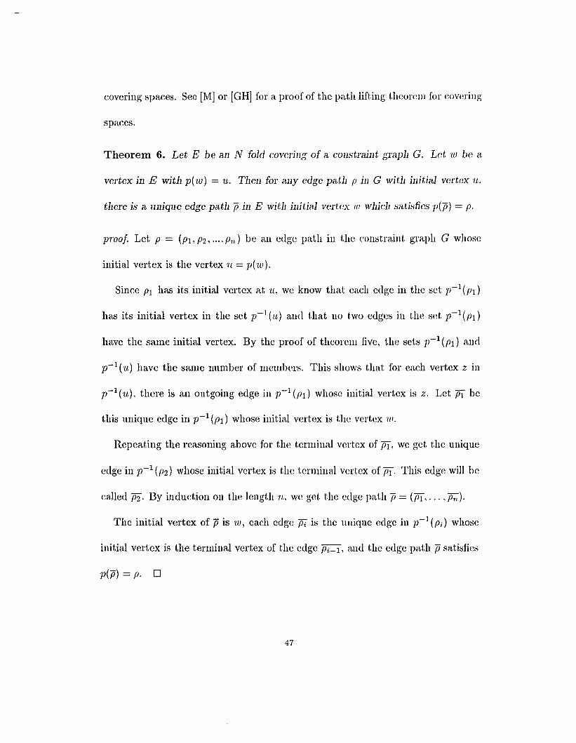
Theorem 6. Let E be an N fold covering of a constraint grapb G. Let in be a

vertex in E Wit11 p(w) = 'It. Tlieu for <tny edge path P in G witu initial vertex 'It.

there is a nuiqne edge patll (5 in E wiili iuitiel vertex '/lJ wbicu satisfics p((5) = p.

proof. Let P = (PI, P2, ..., Pn) be an edge path in the constraint graph G whose

initial vertex is the vertex '/1, = p(w).

Since PI has its initial vertex at '11., we know that each edge in the set p-I (PI)

has its initial vertex in the set p-I ('It) and that no two edges in the set p-I (pd

have the same initial vertex. By the proof of theorem five, the sets p-1 (PI) and

p-I (-u) have the same number of members. This shows that for each vertex z in

p-I('U), there is an outgoing edge in p-I(pd whose initial vertex is z. Let PI be

this unique edge in p-1 (PI) whose initial vertex is the vertex 'W.

Repeating the reasoning above for the terminal vertex of PI, we get the unique

edge in p-1 (P2) whose initial vertex is the terminal vertex of Pl. This edge will be

called P2. By induction on the length n, we get the edge path (5 = (PI, . . . •Pn).

The initial vertex of (5 is 'lV, each edge Pi is the unique edge in p-I (Pi) whose

initial vertex is the terminal vertex of the edge Pi-I, and the edge path (5 satisfies

p(p) = p, 0

47

We will refer to this theorem as the edge path lifting theorem. In the next

chapter, the edge path lifting theorem will be important for the construction of

(d, It,) constrained codes from a covering space of the (d. It,) constraint graph.

Recall that a proper edge path P = (PI, ... , Pn) in a constraint graph G is an

edge path for which each edge Pi is a proper edge from G. For a proper edge path

P in a (d, It:) constraint graph, there is an associated (d, h:) constrained sequence

obtained by using the binary labels for the edges in the edge path. The (d. k)

constrained sequence associated with the proper edge path P = (PI, ... , Pn) will

be 3 = (31,'" ,3n ) where 3; is the binary label ill the constraint graph G for the

edge Pi. By the edge path lifting theorem, if ui is a vertex of E with p(w) the

initial vertex of the edge PI, then there is a unique edge path p in the covering

space E whose initial vertex is tu and which satisfies p(p) = p. The edge path

p is determined by its initial vertex and by the (d. It,) constrained sequence which

is associated with the edge path p. This association of edge paths in a covering

space with (d, It,) constrained sequences will be a key in the construction of (d. k)

constrained codes introduced in the next chapter.

We want to consider how the fundamental group of a covering space of a con­

straint graph is related to the fundamental group of the constraint graph. Let E

be a covering space of the constraint graph G and let u: be a vertex in E with

'U = p(w). Suppose p = (PI, ...• Pn) is a reduced edge path in E which is a loop

at 'W. Then the loop p is an element of the fundamental group 1r(E. 'W). We define

48

the mapping p'": n(E.w) --t n(G,u) by p*(p) = (p(PI)'''',P(Pn))' The mapping

p" maps the fundamental group of the covering space to the fundamental group of

the constraint graph.

We want to show that p* is a monomorphism of n( E, 'IV) into n( G, 'U.). If P

and "7 are elements of n(E,w), then their product pT is the reduced edge path

obtained from the edge path p concatenated with the edge path "7. That is. fJT =

(PI,' .. , pn+l-i, Ti, ... , Tm) where 'l is the smallest positive integer such that Ti is

not the reversed edge of the edge Pn+l-i. The mapping p* then satisfies:

(5)

p*(pT) =(p(pt}, 'P(Pn+l-d,P(Td···· ,p(Tm ) )

=(p(pt}, ,P(Pn),P(Td,··· ,p(Tm ))

=p* (p)p* ("7)

Thus showing that p* is a homomorphism.

To show that p* is one-to-one, suppose (j and "7 are reduced edge paths which

are elements of n( E, '/lJ) and which satisfy p*(a) = p*("7) = p. By the edge path

lifting theorem, there is a unique edge path p in E with initial vertex 'llJ and with

p*(p) = p. But the two edge path 0' and "7 have initial vertex 'IV and satisfy

p = p" (0') = p*(7). Thus the two edge paths 0' and "7 must be equal, showing that

p* is one-to-one.

49

We summarize these results in the theorem below.

Theorem 7. Tlio uuippiugp" : 7r(E,w) ---t 7r(G,'U) defined by

(6) p*(p) = (p(pd,··· ,P(Pn))

is a monomorphism of tlie fundamental group 7r(E, 'Ill) of tlie covering space into

the fundamental gJ'OUp 1f(G. 'U) of the constraint graph

This is a well known result for covering spaces. See [M] or [ GH] for a proof of

the general case of this theorem.

2.4 CONSTRUCTION OF COVERING SPACES

FOR. THE (d, k) CONSTRAINT GRAPHS

In this section, a constructive process for building a covering space of a id, I..~)

constraint graph is given. The topological properties of the (d. k) constraint graphs

presented in the previous sections will be used to develop the construction. The

construction of covering spaces presented here follows the the construction pre­

sented in [N].

Let G be a constraint graph. either a (d, k) constraint graph or a (d. (0) con­

straint graph. We start by choosing a splitting complex for the constraint graph.

Recall that a splitting complex K is a subset of the set of midpoints for the edges in

G such that the subgraph of G consisting of the edges in G which do not intersect

K is a maximal tree for the constraint graph G. In the first section of this chapter.

50

some properties of splitting complexes are presented. By theorem three, there are

k +1 splitting complexes for the (d, k) constraint graph and there are d+1 splitting

complexes for the (d, 00) constraint graph. We pick K to be a splitting complex

for the constraint graph G.

Consider the constraint graph G. For each point >. of the splitting complex

K, let e,\ be the edge in the constraint graph which contains the point >. as its

midpoint. We form the figure GK from the constraint graph G by splitting the

edge e,\ at each point>. of the splitting complex K. That is, for each point>. of

the splitting complex K, we break the edge e,\ at the point >.. The direction of the

break is maintained, so that one side of the break is incoming to the break and the

other side is outgoing to the break. The resulting figure, after each point of the

splitting complex K is split, will be the split figure GK .

Let e be a finite set. For the examples we will consider, the set e will be the

integers from 1 to N. or will be a set of binary polynomials. Let N be the number

of elements in the set e. The covering space to be constructed using the set e will

be an N fold covering of the constraint graph G. The set ewill be used as labels

for the N copies of the split figure GK. The covering space is obtained by gluing

the N copies of the split figure GK together.

To build the covering space from the N copies of the split figure GK , we need a

set of permutations 011 the set e. For each point>. of the splitting complex K. we

pick a permutation P>. from the symmetric group on the set e. The permutation ]1,\

51

will be called the permutation associated with the point A of the splitting complex

K.

The permutations PA are chosen so that the subgroup generated by the set

{PAIA E K} is a transitive subgroup of the symmetric group on the set e. A

subgroup H of the symmetric group on the set e is a transitive subgroup if for

each pair 'Y and ti of elements from e. there is a permutation in the subgroup

H which sends 'Y to 8. See [J] for more on transitive subgroups. The condition

that the subgroup generated by the permutations {PAIA E K} be a transitive

subgroup ensures that the constructed covering space is a connected graph. A

set of permutations {PAIA E K} from the symmetric group on the set e, which

generates a transitive subgroup, will be called a set of defining permutations for

the splitting complex K.

We want to build an N = lei fold covering of the constraint graph G. The

construction process is taken from [N], where it is done in greater generality, To

build a covering space of G, we start by taking N copies of the split figure GK . We

label the copies of the figure GK using the set e. The set of defining permutations

{PAjA E K} is used to reconnect tho split figures GK . The permutation PA is used

as a guide for which levels to glue together for the break at the point >. of the

splitting complex K. That is, we identify the incoming side of the break at the

point >. in the figure labeled by the element 'Y with the ontgoing side of the break

at the point A in the figure labeled by the element b, whenever the permutation

52

PA sends the element 'Y to the element 8. This process of identifying sides of the

breaks at the N copies of the point>. is continued until the breaks at all the copies

of the point ,,\ have been reconnected. We repeat this process for all the points of

the splitting complex K. The resulting figure, after all the split edges have been

reconnected, is a connected graph, which we call E.

The graph E, constructed in the manner above, is an N fold covering of the

constraint graph G. We summarize the results of the construction in the theorem

below.

Theorem 8. To every set of defining permutations for a splitting complex K of

the constraint grepl: G, there corresponds a covering spece E of the constraint

graph G.

]JTOo]. The construction of the graph E is described in the paragraphs above. The

graph mapping P of E onto G sends each level of the split figure GK onto the

constraint graph G in the natural way. It can be verified that p satisfies the

conditions in the definition of a covering space. 0

In the covering space E, the defining permutations {PA/"\ E K} are used as

a guide for which levels of the split figure GK to glue together at the points of

the splitting complex K. We want to define a mapping of the fundamental group

1r(G,u) into the group of permutations generated by the set of defining permuta­

tions. To define the mapping, recall that each element p of the fundamental group

53

7r(G, 'u) can be written as a product Q~I 0:';2 •• , a~m where Q>. is the loop at '/L as-/\};'\2 Am I

sociated with the point Ai of the splitting complex K and e, is either -lor 1. Wc

where p is equal to the product Q~l a~2 ... a~TIl . The mapping 4' is a group homo-1\1 "'2 Am

morphism.

We use Pp to represent the permutation 4'(p), The permutation Pp will be called

the permutation associated with the edge path p.

Lemma 9. Let p be an edge patil in 7r( G, 'It) and let p be an edge patil lifting of

the edge peili p to tile covering space E. If tile initial level ofp is tile level labeled

by /, then the terminal level of p will be tlie level labeled by Pp(r). where Pp is

tlie permutation sssocieted witli tile edge pei]: p,

proof. Notice that the first time the edge path p crosses a point of the splitting

complex K, the edge path p goes from the level labeled by / to the level labeled

by p~\ (r). This process repeats for each point of the splitting complex K that the

edge path p crosses, giving that the edge path p goes from the level labeled by /

to the level labeled by p~m p~rn-l " .p~2 p~l (r). But this is exactly the action of theAm Am -1 /\2 Al

permutation Pp on /. 0

This lemma is useful for finding the fundamental group 7r( E, '/l1) of the covering

space E constructed above. Suppose / is the clement from the set f) used as a label

for the level which contains the vertex ui. We take S to be the set of clements

54

from the fundamental group 7f(G, 'u) whose associated permutations fix the label

'Y. That is, s is in the set S if and only if P,~(f) = 'Y where P, is the permutation

associated with the edge path s. The set S is a subgroup of the fundamental group

7f(G,'u). We want to show that the fundamental group 7f(E,w) is isomorphic to

the subgroup S.

Recall that the group homomorphism p* induced by the graph mapping p is

a monomorphism of the fundamental group 7f(E, 'W) into the fundamental group

7f(G,'/1.). We show now that p* is an isomorphism between the subgroup S and the

fundamental group 1r(E, w).

Consider an edge path p in the subgroup S. By the edge path lifting theorem,

there is a unique edge path p in E with initial vertex 'Wand with p* (p) = p. By the

lemma, p will end in the level labeled by Pp(f). Since p is in the subgroup S, this

gives PrA'Y) = 'Y. The vertex on the level labeled with 'Y and in the set p-l(n) is

the vertex 'W. This shows that p is a loop at the vertex wand so S C p" (7f( E, w)).

Now consider an edge path Ii in 7f( E, 'W). Since 75 begins and ends on the level

labeled with 'Y, the lemma implies that the permutation associated with p*(p) will

fix the label 'Y. This is the condition for p* (p) to be in the subgroup S and so

p*(7f(E, w)) c S.

This completes showing that the subgroup S is isomorphic to the fundamental

group 7f(E, w). We summarize this below.

55

Theorem 10. Tile Iuudesueutel group 1f( E, 'IV) of tile covering space E coustructed

above is isomorphic to tile subgroup 8 of tile Iutuuuucntel group 1f( G, 'lL) wucte S

consists of the edge paths wiiose associated permutations fix the label, of the level

whicu contains the veriex ui.

Suppose 8y is a right coset of the subgroup 8 = p* (1f( E, 'Ill)) in the fundamental

group 1f(G,'u). Consider two elements 819 and 829 of the right coset, with PSlf!

and P,~2g being their associated permutations. If 'Y is the label for the level which

contains the vertex 'W, then P,~lg(f) = PgPs 1 (,) = Pg(, ) = PgP'q 2('Y ) = P.~2g(f).

This shows that the associated permutation for each edge path in the coset Sf] will

send the label , to the label Pg (,).

Now consider the two right cosets Sli and 8y of the subgroup S. Suppose that

the associated permutations for two elements 819 and 8211. from the respective coscts

satisfy P.~lg(f) = PS2h(f). Then it follows that Ps1gb) = P'Q2hb) = P/iP S2('Y) =

Ph(')· Or by rearranging that 'Y = p,-;1P,9Iyb) = Ph-IP.~lg(f) = P'qlf/h-I(,). This

shows that the permutation associated with the edge path sl,qh- 1 fixes the Iabel y.

Thus, the edge path slgh-1 is in the subgroup S. That is, 8gh-1 = 8 or Sg = 811.,

showing that the two cosets are equal.

We have shown that the cosets of the subgroup 8 are determined by the action

of their associated permutations on the label 'Y. We summarize the two previous

paragraphs in the theorem below.

56

Theorem 11. For each :1; E e. tlie set of edge paths in 7r( G. 'u) which have associ­

ated permutations tllat send I to the label x will be a right coset of tile subgroup

s = p*(7r(E,w)).

These two theorems will be used when we examine the constrained codes con­

structed from the covering space E.

To conclude this section, we present an example of the construction of a covering

space. We begin with the (1,3) constraint graph G. The splitting complex J( will

be the midpoints of the three edges that are incoming to the vertex aI. It is dear

that J( is a splitting complex for G, as the subgraph of G which does not intersect

J( is a maximal tree for G. We label the points of the splitting complex J( as a,

(3, and 8. The edges in the (1,3) constraint graph are split at the points a, (3, and

I) to give the split figure GK . The split figure GK is shown below.

Figure 2.3: Split Figure GK

57

The set e used to index the levels of the split figure GJ( will be the integers from

one to four. The defining permutations will then be from the symmetric group

34 , We choose the defining permutations as Po. = (1. 2, 3), Pf3 = (1. 2)(3, 4), and

Po = (2,3). The defining permutations are used to connect together the four copies

of the split figure GJ( together.

To reconnect the four copies of the point a, we use the permutation Po. = (1,2,3).

This is done by identifying the incoming side of the break at al with the outgoing

side of the break at a2, identifying the incoming side of the break at a2 with the

ou tgoing side of the break at (}:3, and identifying the incoming side of the break at

a3 with the outgoing side of the break at al. The incoming side and outgoing side

of the break at a4 are identified.

This process of reconnecting the split edges is repeated for the points (3 and 8

using the permutations P(3 = (1. 2)(3, 4) and Po = (2,3). The resulting graph E is

shown below. The graph E is a four fold covering of the (1,3) constraint graph.

58

Figure 2.4: Four Fold Covering of (1,3) Constraint Graph

5D

2.5 CONCLUSION

In this chapter, the topological properties of the (d, k) constraint graphs and

of the (d, (0) constraint graphs are examined. The first section deals with the

fundamental group of a constraint graph. The second section deals with covering

spaces of constraint graphs. The final section contains a construction for building

covering spaces of a constraint graph. This chapter is intended as an introduction

for the nonexpert to some basic topological facts about constraint graphs.

60

Chapter 3

(d, I.~) Constrained Block

Codes From Covering Spaces

3.1 INTRODUCTION

In this chapter, (d, k) constrained codes constructed from covering spaces of

the (d. I.:) constraint graph are examined. Examples of (d, I.:) constrained codes and

id, (0) codes are given. Systematic codes for detecting all single errors are given for

possible applications. In the final section, the average probability of an undetected

error for the family of systematic (d, k) constrained block codes is shown to decrease

exponentially.

3.2 INTRODUCTION TO (d, k) CONSTR.AINED BLOCK CODES

The (d, k) constrained codes and the (d, (0) constrained codes were introduced

in the first chapter. We will use the term "constrained code" to mean either a

id: k) constrained code or a (d. (0) constrained code.

A practical method for constructing constrained codes in given in [ACH]. An

excellent introduction to these codes is given in [Silo The constrained codes they

construct are called sliding block codes. Other constructions of constrained codes

are given in [TB] and [Lee].

61

The conventional coding scheme in magnetic recording concatenates an error-

control code with a constrained code. For instance. see [HHW]. The input binary

sequence is first encoded using an error-control code. The encoded sequence is then

further encoded using a constrained code to obtain a constrained sequence. The

constrained sequence is then sent to the channel. A diagram of this coding scheme

is shown below.

Error Constraint- Control - CodeCode Encoder

, r

channel

ECC Constraint... Decoder Code --- Decoder -

Figure 3.1: Conventional Coding Scheme

The sequence received from the channel is first decoded using the constrained

code decoder. This gives an unconstrained sequence which is then decoded using

the error-control code decoder. The binary sequence obtained from the error-

control code is an estimate of the original input sequence.

62

As noted in [HHW], this coding scheme is not entirely satisfactory. The problem

IS that for all known constrained codes, errors which occur in the channel are

multiplied by the constrained code. The constrained code decoder will turn a single

error into a burst of errors. This is an undesirable property. The codes presented

in this chapter are an attempt to alleviate this difficulty with the standard coding

scheme.

The codes that we will construct are (d, k) constrained block codes. A (d. k)

constrained block code is a set of (d, /':) constrained sequences of fixed length n

such that for any pair of code sequences x and y, the length 211, sequence obtained

by concatenating x onto y will be a (d, k) constrained sequence. See [LW] or [FL]

for examples of (d, k) constrained block codes. We present some new constructions

for (d, k) constrained block codes.

We will also consider (d, 00) constrained block codes. The definition will be the

same as for the (d, k) constrained block codes. The term "constrained block code"

will be used to mean a (d, k) constrained block code or a (d. 00) constrained block

code.

The idea is to construct constrained block codes which provide some error pro­

tection against errors which occur in the channel. In [H], the errors which occur in

magnetic recording are analyzed. The errors are categorized as either shift errors,

drop in errors, or drop out errors. A shift error is said to occur when a one in the

i t h position is shifted to the i-I th position or to the i + 1th position. A drop in/out

63

error is said to occur when a one is changed to a zero or a zero is changed to a one.

In magnetic recording, shift errors and drop in/out errors occur simultaneously.

The shift distance between two constrained sequences will be the minimum num­

ber of shift errors required to change one sequence into the other. Similarly. the

Hamming distance between two constrained sequences will be the minimum num­

ber of drop in/out errors required to change one sequence into the other. The

minimum shift distance of a constrained block code will be the minimum shift

distance attained by considering all possible pairs of nouequal code sequences.

Similarly, the minimum Hamming distance of a constrained block code will be the

minimum Hamming distance attained by considering all possible pairs of nonequal

code sequences.

For each code presented in the next section, we will give its minimum shift

distance and its minimum Hamming distance.

3.3 BASE POINT CODES

In chapter two, covering spaces for the (d, k) constraint graphs were introduced.

We want to usc covering spaces of a (d, k) constraint graph to construct (fl, k)

constrained block codes. Before proceeding, we review the relavent facts about

constraint, graphs and covering spaces.

To each proper edge path in the (d, k) constraint graph, there is an associated

(d, k) constrained sequence obtained by using the binary labels of the edges in the

64

edge path. Suppose E is a covering space of the constraint graph G. By the edge

path lifting theorem, to each edge path p in the constraint graph whose initial

vertex is 'IL, there corresponds. for each vertex ui in »:' ell), a unique edge path p

in the covering space E such that the initial vertex of p is wand p* (p) = p. The

fundamental group 1f(G, u) is the set of reduced edge paths in the constraint graph

G which are loops at the vertex u. The set of proper edge paths in the constraint

graph which are loops at the vertex u is a subset of the fundamental group 1f( G, u).

For constructing the base point codes from a covering space E, we use the fact

that to each (d, k) constrained sequence associated with a proper edge path from

1f(G, 'IL), there is a unique edge path in the covering space with a specified initial

vertex.

Definition 1. Suppose E is a covering space of the (d, k) constraint gtepli G and

let w be a vertex in the E witu p(w) = u. The lengtli n. basc point code for the

covering space E at the vertex 'W is the set of (d, k) constrained sequences associated

with the set of proper edge pnth« in the fundamental group 1f(G, u) wliiclt lift to

edge petus in tile coveting E t1lat are loops at the vertex 'W.

We will also consider base point codes for covering spaces of the (d, (0) con­

straint graphs. The definition of base point codes for covering spaces of the (rl, (0)

constraint graph will be the same as the definition of base point codes for covering

spaces of the (d, 11,) constraint graph.

65

For a base point code, we use C to represent the set of constrained sequences

that comprise the code, C to represent the set of proper edge paths from 7r(G.'u)

whose associated sequences form the code C, and C to represent the edgc paths in

the covering space E determined by lifting the edge paths in C.

The definition of the base point codes for a covering space says that C is the set

of constrained sequences such that C is a subset of the fundamental grou p 7r(E. 'Ill)0

We want to consider some examples of base point codes for covering spaces of

the (d, k) constraint graphs and of the (d, 00) constraint graphs.

Before proceeding, we review some facts about the construction of covering

spaces for constraint graphs.

Recall that a covering space E of a constraint graph G is determined by a set

of indices e and a set {PAIA E K} of defining permutations for a splitting complex

K of the constraint graph. The permutations PA are chosen from the symmetric

group on the set eo The covering space E will be a lei fold covering of the constraint

graph Go See chapter two for the details of the construction.

The splitting complex used in the construction of a covering space of a (d. /,~)

constraint graph will be taken to be the midpoints of the k - d +1 edges that are

incoming to the vertex alo The splitting complex used in the construction of a

covering space of a (d, 00) constraint graph will bc taken to be the midpoints of

the two edges that are outgoing to the vertex ad+lo These conventions are made

to make the analysis of the constructed covering spaces easier.

66

As a first example, we construct a length twelve (1,2) constrained block code

which is a base point code for a. three fold covering of the (1. 2) constraint graph.

The set e is taken to be the integers from one to three. The set of defining permu­

tations is taken from the symmetric group 8 3 . Let 0: be the midpoint of the edge

from vertex 0,2 to vertex 0,1 and let f3 be the midpoint of the edge from vertex 0,3 to

vertex 0,1. The defining permutations are chosen as Pc< = (1. 2) and P13 = (2. 3). The

set {Po, P13} is a set of defining permutations for the splitting complex K = {0:,,6}.

The three fold covering constructed with the set {Pa, P/3} is shown below.

Figure 3.2: Three Fold Covering of (1,2) Constraint Graph

We consider the base point code at the vertex 'W. where '/lI is the vertex 0,1 in the

level of the covering space indexed by a one. The length twelve base point code

67

at 'IV will consist of the five (1. 2) constrained sequences whose corresponding edge

paths in the covering space are loops at the vertex ui. The base point code C is

shown below:

c= {OlOlOlOlOlOl,OlOlOOlOlOOl.OOlOlOlOlOOl(1)

OOlOlOOlOlOl,OOlOOlOOlOOl}

. . log2/ C!The rate of the base point code C IS R = = .1934, its minimum shift

12

distance is two, and its minimum Hamming distance is three. For comparison. we

note that the capacity of the (1,2) constrained codes is .4057.

As a second example, we construct a length eight (0.2) constrained block code

which is a base point code for an eight fold covering of the (0,2) constraint graph.

The set e is taken to be the integers from one to eight. The set of defining pcrum-

tations is taken from the symmetric group S8. Let a be the midpoint of the edge

which is a loop at the vertex aI, let fJ be the midpoint of the edge from vertex a2 to

vertex al. and let I be the midpoint of the edge from vertex a3 to vertex al' The

defining permutations are chosen as Per. = (1,2,3,4.5.6.7), Pf; = (1, 2, 7, 3. 8, 5, 4),

and p-y = (1,2,6,4,3,5,8). The set {Per.,Pr;,P-y} is a set of defining permutations

for the splitting complex K = {a, fJ, I}' The eight fold covering constructed with

the set {Per., Pf3, p-y} is shown below.

68

...---......aJ----....~

Figure 3.3: Eight Fold Covering of (0,2) Constraint Graph

69

We consider the base point code at the vertex ui. where ut is the vertex 0,1 in

the level of the covering space indexed by a one. The length eight base point code

at 'W will consist of the ten (0.2) constrained sequences whose corresponding edge

paths in the covering space arc loops at the vertex 'W. The base point code C is

shown below:

C = {OI111111.01010011,OI101001,OOI0011I,10111011(2)

11001111,11011001,10101101.10010111.11110101}

The rate of the base point code C is R = log~ ICI = .4152. its minimum shift

distance is three, and its minimum Hamming distance is three. For comparison.

the capacity of a (0,2) constrained code is .8792.

As a third example, we construct a length seven (0,00) constrained block code

which is a base point code for an eight fold covering of the (0.00) constraint graph.

The set () is taken to be the set of binary polynomials whose degree is less than

three. The set of defining permutations are taken from the symmetric group on the

set of binary polynomials whose degree is less than three. Let a be the midpoint

of the edge labeled with a one and let (3 be the midpoint of the edgo labeled with

a zero. The defining permutations are chosen as:

Pc. :11,0 + h1x + h2x 2-t (1 + 11,2) + (11,0 + h2 )J:+ 11. 1;[; 2

(3)

PfJ :11.0 + h1x + h2 J;2 -t h2 + (ho + h2 )x + h1:r; 2

The set {Pc., P.e} is a set of defining permutations for the splitting complex

J( = {a, (3}. The eight fold covering of the (0. 00) constraint graph is shown below.

70

Figure 3.4: Eight Fold Covering of (0,00) Constraint Graph

We consider the base point code at the vertex 'W, where 'Ill is the vertex labeled

with the zero polynomial. The length seven base point code at the vertex in will

consist of the sixteen binary sequences whose corresponding edge paths in the

covering space are loops at the vertex 'W. The base point code C is shown below:

C = {0000000,0001011,0010110,0101100,1011000,0110001,

(4) 1100010.1000101,1101001,1010011,0100111.

1001110,0011101,0111010,1110100,1111111}

71

The rate of the base point code C is R = log~ICI = 4/7, its minimum shift

distance is three, and its minimum Hamming distance is three. The base point

code C is the well known Hamming [7,4] cyclic code.(See [Lej, [PW], or [SM])

The examples above show that a base point code for a covering space of the

(d, I.:) constraint graph is a (d. I.:) constrained block code. We prove this now.

Theorem 1. Suppose C is ;L base point code for <L covering' spec» of the (d. k)

constraint graph. Then C is a (d, I.:) constrained block code.

proof. We need only show that C satisfies the concatenability condition. Suppose z

and y be sequences in the base point code C and with x and y their associated edge

paths in7r(G, ·u). Since the edge paths x and yare proper edge paths, their product

xy will also be a proper edge path. The (d, k) constrained sequence associated with

the proper edge path xy will be the sequence x concatenated by y. This shows

that the base point code C is a (d, k) constrained block code. 0

The third example above showed that the Hamming [7,4] cyclic code is a base

point code for an eight fold covering of the (0,00) constraint graph, We show in

theorem two that an [n, k] cyclic code is a base point codc for an 211-

k fold covering

of the (0,00) constraint graph. Before proving the theorem. we review some basic

facts concerning cyclic codes.

A binary polynomial has an associated binary sequence obtained by taking the

coefficients of the polynomial. An ['11" kJ cyclic code C has a distinguished binary

72

polynomial g(x) of degree n - I.:. The polynomial g(x) is called the generator

polynomial of the cyclic code. The code C consists of the length ti binary sequences

whose associated binary polynomials are divisible by g(x). See [LC], [PW] , or [SM]

for a comprehensive treatment of cyclic codes. A further note is that the generator

polynomial g(x) divides the polynomial x n + 1.

Theorem 2. An [n, k] cyclic code is a base point code for a 2n - k fold covering of

the (0, (0) constrain t grepli.

proof. Suppose g(x) is the generator polynomial of an [n, k] cyclic code C. We use

g(x) to get a set of defining permutations. The set e used to index the levels of

the covering space is taken to be the set of binary polynomials of degree less than

2n - k • The set of defining permutations are taken from the symmetric group on the

set of binary polynomials whose degree is less than 2n-

k . Let n be the midpoint

of the edge labeled with a one and let (3 be the midpoint of the edge labeled with

a zero.

The defining permutations are chosen as:

Po: :h(x) ---+ x· h(x) +hn - k - 1 . g(x) + 1 modulo ;r;n-k

(5)

P/3 :h(x) ---+ x· h(x) + hn - k - 1 • g(x) modulo xn -k

where hn - k - 1 is the coefficient of xn - k - 1 in h(x).

73

To see that these mappings are actually permutations on the set of binary poly­

nomials of degree less than ri - k, suppose that two polynomials '1'(:[;) and q(:c) are

sent to the same state by POI.' That is, r( x) and q(:z:) satisfy:

(6) u:> r(x) + '''71.-k-1 . g(x) + 1 = x· q(x) + q71.-I.:-1 . g(x) + 1 modulo :z:n-k

or rearranging gives:

(7) x' (q(:r;) - ',,(x)) + (qn-k-l - '''n-k-1)' g(x) = 0 modulo :cn-

k

Now consider the two cases, whether qn-k-1 = rn-k-l or qn-k-l =f. Tn- k- 1.

First, if qn-k-1 = 7'n- k- l , then equation seven reduces to ;r; . (q(x) - 7'(;r;)) =

omodulo xn-k. The polynomial q(x)-r(x) has degree less than '11,-1.:-1, since their

leading coefficients are equal. So, the equation x· (q(:r:) - T(:C)) = 0 modulo ,Tn- k

implies that the polynomial q(x) - T(X) is zero. Showing that q(:c) = 7'(X).

If qn-k-1 =f. rn-k-l, then equation seven reduces to :c· (q(x) - T(X)) + g(x) =

omodulo x n - k . Since g(x) divides x n +l , its constant term is one. The polynomial

x· (q(,T) - p(x)) has constant term zero. Thus the left side has constant term one,

hut the right side has constant term zero. This contradiction shows that this case

call not occur.

Hence, we have that POI. is a permutation OIl the set of binary polynomials whose

degree less than n - k. The proof that P!3 is a permutation is the same as the

proof for Pa' Thus, we have that {POl' Pld is a set of defining permutations for the

splitting complex {a.{3}.

74

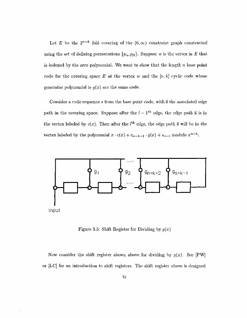
Let E be the 2n - k fold covering of the (0, (0) constraint graph constructed

using the set of defining permutations {Pa,P,B}' Suppose 'W is the vertex in E that

is indexed by the zero polynomial. We want to show that the length n base point

code for the covering space E at the vertex 'IV and the ['17.,1.:] cyclic code whose

generator polynomial is g(x) are the same code.

Consider a code sequence s from the base point code, with s the associated edge

path in the covering space. Suppose after the 1- 1til edge, the edge path s is in

the vertex labeled by c(x ). Then after the [til edge, the edge path s will he in the

vertex labeled by the polynomial x· c(x) + Cn-k-l . g(x) + 87/-1 modulo x n-

k.

input

Figure 3.5: Shift Register for Dividing by g(x)

Now consider the shift register shown above for dividing by g(x). Sec [PW]

or [LC] for an introduction to shift registers. The shift register above is designed

75

to divide bit by bit, the input polynomial by g(:r:). After the coefficients of a

polynomial 11,( x) are input, the contents of the shift register will be the remainder

of h(x)jg(x). Suppose the contents of the shift register, after the l - Ith input bit

are c(x). Then, after the lth input bit, the contents of the shift register will be

;E' c(x) + Cn-k-l . g(x) + hn-l modulo x n-

k.

Comparing the two previous paragraphs shows that the contents of the shift

register correspond to the state in the covering space that the edge path is in.

Since a sequence is in the base point code when its associated edge path is a loop

at the vertex ui, we see that a sequence from the base point code when inputed

into the shift register will put the contents of the register to zero. This is the same

condition for a sequence to be in the cyclic code generated by g(x). Therefore, the

two codes are the same. 0

The example of the Hamming [7,4] cyclic code above is derived using this the-

orem.

The covering space E constructed in the theorem will be called the cyclic cov­

ering generated by g(x).

3.4 PARITY POINT CODES

A base point code for covering space E is a set of (d, h:) constrained sequences

whose associated edge paths in E arc loops at a specified vertex. We get different

codes if the edge paths are required to connect two specified vertices. Suppose 'W

76

and z are two vertices in the set p-l(n). We get a (d, k) constrained block code

by taking the (d, l.~) constrained sequences whose associated edge paths have initial

vertex wand terminal vertex z.

Definition 2. Suppose E is a covering space of ilie (d, I.:) constraint gtnpl: G and

let io and z he a two vertices ill the set p-l('U). Tile leugtli ti parity point code

for tile covering space E from tu to z will he the set of (d, k) constrained sequences

whose associated edge peih« in E llave initial vettex ui and terminal vertex z.

As usual, the definition for the (d, 00) constrained sequences will be the same,

We note that the base point codes are parity point codes where the initial vertex

and the terminal vertex are the same. We now consider some examples of parity

point codes.

As a first example, we consider the eight fold covering of the (0,2) constraint

graph that was used in the second example above. The initial vertex is chosen

to be the vertex alan the level indexed by one. The code length is chosen to bc

eight. The various parity point codes are listecl below by the terminal vertex used

to generate the code. We usc aij) to represent the vertex a, on the level j.

77

Parity Point Codes

Table 3.1: Parity Point Codes for E Covering of the (0,2) Constraint Graph

Terminal

Vertex

ap) {01111111, 01010011,01101001,00100111, 1011101l.

11001111,11011001,10101101,10010111.11110101}

a~2) {00110111,01111001,11110011,11100101, 11011111,01101111.

01010101,11001001,10101011,11011111,10111101}

a~3) {IOII0111.11111001.01100101,01011111,00101011,10011011.

11010101,01110011, 11101111,00111101,01001001}

a~4) {00101101, 01011001,11111111,00111011. 0111010l.

11101001,11010011,10100111,01001111.10011101}

a~5) {11010111,11101101,10011001,00111111,01001011,

11111011,10110101,00101001,01100111,01011101}

a~6) {01110111,01001101, 00111001. 10100101, 10011111,

11101011,01011011,10110011,00101111, 11111101}

a~7) {11110111, 11001101, 10111001,00100101,01101011,

10010101,00110011,10101111,01111101}

a~8) {01010111, 01101101,10111111,11001011, 0111101l.

00110101,10101001,10010011,11100111. 11011101}

78

The parity point codes vary in size from nine to eleven code sequences. Each

parity point code has shift distance at least three and Hamming distance at least

three. The code rates range from .3962 to .4324. For comparison, the capacity of

a (0,2) constrained code is .8792.

There are eighty-one sequences of length eight which satisfy the (0,2) constraints

and whose associated edge paths in G are loops at the vertex al. The parity point

codes partition these sequences into eight disjoint subsets.

As a second example, we consider the eight fold covering of the (0,00) constraint

graph that was used in the third example above. The initial vertex is chosen to be

the vertex indexed by the zero polynomial. The code length is chosen to be seven.

For each vertex in the covering, we get a different parity point code. The parity

point code with the terminal vertex being the vertex indexed by the polynomial :r:

is shown below:

(8)

C = {0000010,0001001,0010100,0101110,1011010,0110011,

1100000,1000111,1101011,1010001,0100101,

1001100,0011111,0111000,1110110,1111101}

The parity point code is a coset of the Hamming [7,4] cyclic code. The rate of

the code is 4/7, its minimum shift distance is three, and its minimum Hamming

distance is three. The covering space of this example is the cyclic covering generated

by g(:1:) = x 3 +:1: + 1.

79

The parity point codes for the cyclic covering generated by a polynomial g(:r:)

will always be the cosets of the cyclic code generated by g(x). As a corollary of

theorem two, we prove this fact. The idea is that the index of an edge path's

terminal vertex in the covering space determines the coset the binary sequence will

be in.

Corollary 3. Suppose E is tile cyclic covering generated by g(x). Let 11,( J:) be

a polynomial of degree less than n - k and let 11, be the leugtli 17, sequence corre-

spotiditig to 11,( x). Then the parity point code from the vertex indexed by tlie zero

polynomial to the vertex indexed by 11,( x) will be the coset 11, +C of tile cyclic code

C generated by the polynomie! g(x).

proof. Suppose s is a sequence from the parity point code. In the proof of theorem

two, it was shown that the state polynomial h(x) of the terminal vertex for the

edge path s is the remainder from dividing the polynomial s(x) by the generator

polynomial g(x ).

Consider the coset h-e C of the cyclic code C generated by g(x). Suppose h s-c is

a sequence from this coset. Since g(;1;) divides the polynomial c(:c) and the degree

of h(x) is less than the degree of g(x), we see that the remainder of the division

h(x)+c(x) mb· I ( )g(x) WI e), x .

This shows that the parity point code and the coset 11, +C are the same. 0

80

The examples above show that the parity point code for a covering of the (d. k)

constraint graph are (d, /':) constrained block codes. The proof of this is the same

as the proof of theorem one. We omit repeating the proof.

Theorem 4. Suppose C is a parity point code for a covering of the (d, k) constraint

graph. Tlieu C is a (d, k) constrained block code.

We want consider what conditions on the covering space ensure that an error in

transmission will be detected by the parity point codes for the covering. Consider

the covering E of the (d, k) constraint graph G, constructed with the standard

splitting complex K and the set {p>.l>' E K} of defining permutations. In chapter

two, we showed that each edge path x in the fundamental group 7f( G, tt) has an

associated permutation Px , formed as a product of the defining permutations.

Suppose x is the edge path in E which has initial vertex on the level indexed

by , and which satisfies p(x) = x. By theorem eleven of chapter two, the edge

path x has its terminal vertex on the level indexed by Px(f). We use this fact to

show which errors are detected by the parity point codes for the covering space E.

Lemma 5. Suppose x and y arc two proper edge paths in 7f(G,'It) such that the

peimutetiou p;-l Py is fixed point free. Then the error pattern wliicli changes the

sequence x into the sequence y will be detected for all parity point codes for the

covering space E.

81

proof. Suppose axb and ayb are two sequences in the same parity point code. where

axb is the sequence a concatenated by the sequence x, which is further concatenated

by the sequence b. Then the permutations associated with the cdge paths axb and

ayb will satisfy P(Lxb(f) = PayfA'y) , where i is the index of the initial vertex of

the parity point code. This becomes PbPxP(L(ry) = PbPyPa(f). and rearranging

Pa(i) = p;lPyPa (, ). Showing that the permutation r;' Py has a fixed point at

Thus, if we assume that pJ-; l Py is fixed point free. then it follows that no two

sequences of the form axb and ayb will be in the same parity point code for the

covering E. Hence, the error pattern that changes the sequence x into the sequence

y will be detected. 0

This lemma shows that parity point codes are natural for detecting errors. In the

next section, we construct practical codes for dctecting all single errors. Leuuna

five will be used to help choose the defining permutations for constructing the

covermg space.

3.5 ERROR. CHECK CODES

In practice, systematic codes are generally preferred. The idea of a systematic

code is as follows. An input sequence of length l is encoded by concatenating a

length 7' sequence onto it. The length l input sequence is called the information

and the length 7' sequence used to concatenate is called the parity. To decode

82

the received sequence, the sequence is checked to see if it is a code sequence. If

the received sequence is a code sequence, then the parity is discarded to give the

estimate of the information. The ease of encoding and decoding makes systematic

codes popular.

We want to construct systematic td, /':) constrained block codes which will detect

all single errors. We want to detect shift errors and to detect drop in/out errors.

The idea is to construct a covering space E of the (d, k) constraint graph such that

the parity point codes for the covering are single error detecting. The systematic

(d, k) constrained block code will be chosen as a subset of a parity point code for

E.

We take Qi to be the loop in G at the vertex al determined by the sequence

of i zeros followed by a one. We express the single error patterns in terms of the

Qi'S. The drop out errors which do not violate the (d, k) constraints will change the

sequence associated with the edge path QiQj into the sequence associated with the

edge path Qi+J+l. The drop ill errors which do not violate the (d,k) constraints

will change the sequence associated with the edge path Qi+j+l into the sequence

associated with the edge path QiQj. The shift errors which do not violate the (d, l,:)

constraints will change the sequence associated with the edge path O'.iQj into the

sequence associated with the edge path Q'i-l Qj+l or associated with the edge path

83

We use lemma five to find conditions on the defining permutations for the parity

point codes to be single error detecting. The drop out errors will be detected if the

permutations of the form P;;:~~jPCti+J+l are fixed point free. The drop in errors will

be detected if the permutations of the form p;:l. Po ·o · are fixed point free. The~I+)+l .)

shift errors will be detected if the permutations of the form P~~:tjPOi-laJ+l and of

We can reduce the number of single error detecting conditions by setting Pi = a

for i even and Pi = b for i odd. The drop out errors will be detected if permutations

of the form a-2b, a-1b-Ia, and b are fixed point free. The drop in errors will be

detected if same permutations are fixed point free. The shift errors will be detected

if permutations of the form a-2b 2 and a-1b-1ab are fixed point free.

We want to find permutations a and b which satisfy the five conditions above.

Consider a = (2,3) and b = (1,2,3). The permutations desired to be fixed point

free are then a-2b = (1,2,3), a-Ib-1a = (1,2,3), b = (1, 2, 3), a-2b2 = (1, 3, 2),

and a-Ib-Iab = (1,3,2). Thus, setting POi = (2,3) for i even and Pa ; = (1.2,3)

for i odd, all the single error detecting conditions will be satisfied.

We use the set {Pa i Id ::; i ::; h:} to construct a three fold covering of the (d. k)

constraint graph G. Suppose J( is the standard splitting complex of the (d. k)

constraint graph. The intersection of the splitting complex J( with the edge path

a; will be the midpoint of the edge ai+l ---? al' This associates a permutation from

the set {Pa i Id ::; i ::; k} with each point of the splitting complex J(. So, the set

84

{Pet; Id :S i :S k} is a set of defining permutations for the splitting complex K. By

the construction process from chapter two. we can build a three fold covering E

of the (d, k) constraint graph using this set of defining permutations. We call this

covering the error check covering for the (d, k) constraint graph.

Theorem 6. Suppose E is tlie enol' check covering for the (d, k) constraint gtepl:

and suppose C is a parity point code for E. Tlieu the code C will detect all single

errors.

proof. By lemma fivc and the discussion above, the theorem follows. 0

As noted earlier, we want to construct systematic codes which are a subset of a

parity point code for E. We consider some examples for the (1,3) constraint graph,

for the (2, 7) constraint graph. and for the (1,7) constraint graph.

As a first example, we consider the (1,3) constraint graph. There are three shift

errors, one drop in error, and one drop out error which do not violate the (1,3)

constraints. The error check covering is constructed using the standard splitting

complex and the defining permutation Pal = Pa a = (1,2,3) and P(:>2 = (2,3). We

show the error check covering below.

85

Figure 3.6: Error Check Covering for (1,3) Constraint Graph

We want to construct a systematic id; k) constrained block code using the error

check covering. The parity is chosen so that each edge path associated with a code

sequence is a loop at the vertex alan the level indexed by a one. The resulting

code will then be a subset of the base point code at the vertex al on the level

indexed by a one. Thus, by theorem six, the code will be single error detecting.

86

Suppose 'W is the vertex 0,1 on the level indexed by a one. To encode au infer-

mation sequence, the edge path associated with the sequence is traced out in the

covering space to find the terminal vertex. The parity is chosen such that each

edge path will be forced back to the vertex 'Ill. The parity length is the smallest

number r such that there is an edge path of length r from every vertex in the

covering to the vertex 'W. The parity length for the (1,3) constrained code is eight.

An encoding table using the error check covering is shown below. We use a~J) to

represent the vertex a; on the level j.

Table 3.2: Error Check Encoder for the (1,3) Constraints

Final State Parity Bits

ap), a~l) 01000101

a~2), a~2) 00101001

(3) (3)0,1 ,0,3 01001001

all) 0,(1) 10101001. 2 ' 4

a~3), ai3) 10100101

(2) (2)0,3 ,0,4 10001001

To decode, the edge path associated with received sequence is traced out in the

error check covering. If the edge path is a loop at the vertex 'W, it is assumed that

no error occurred. The parity is dropped and the estimated information is sent to

the constraincd code decoder. If the edge path is not a loop, an error has been

detected. Corrective measures such as retransmission or rereading can be taken.

87

As other examples, we consider the (2,7) constraint graph and the (1. 7) con-

straint graph. There are twenty-five shift errors, six drop in errors, and six drop

out errors which do not violate the (2,7) constraints. There are thirty-six shift

errors, fifteen drop in errors, and fifteen drop out errors which do not violate the

(1, 7) constraints. The parity length for the (2,7) constrained code will be nine

and the parity length for the (1,7) constrained code will be six. Encoding tables

for the codes arc shown below.

Table 3.3: Error Check Encoder for the (2,7) Constraints

Final State Parity Bits(1) (3) (1) (3) (1)

a1 ,0.2 ,0.3 ,0.4 ' as(2) (2) (2) (2)

0.1 ,0.2 ,0.3 ,0.4

(3) (1) (3)0.1 ,0.2 ,0.3

(1) (1) (1)0.4 ,0.6 ' as

(2) (2) (2) (2)as ,0.6 ,a7 ,as

(3) (3)as ,a7

(3) (1) (3)a6 ' 0.7 ' as

88

001001001

000010001

000001001

100010001

100000001

010000001

100001001

Table 3.4: Error Check Encoder for the (1,7) Constraints

Final State Parity Bits

(P) a(l) a(3) a(l) 0101011 ' 3 ' 5 .. 7

a~2). a~Z), a~2) • aiZ) , a~Z) 000101

a~3), a~3) 000001

(1) (1) (1) (1) (3) (3)aZ ,a4 laG ,as .a5 ,a7 100101

a(3) a(3) a(3) (P) 100001Z ' 4 ' 6 . S

a~Z), a~2) I a~2) 101001

Encoding and decoding for these codes is done ill the same manner as for the

(1, 3) constrained error check code.

The codes presented detect single shift errors and single drop in/out errors. The

ease of encoding and decoding makes these codes practical for applications.

3.6 PROBABILITY OF AN UNDETECTED ERROR FOR THE

SYSTEMATIC (d; k) CONSTRAINED BLOCK CODES

We want now to compute the average probability of an undetected error for the

family of systematic (d, k) constrained block codes. We will get an upper bound

on the probability which decreases exponentially and is independent of the channel

model chosen. The method for this proof is the standard trick of averaging over a

large family of codes.

89

First we discuss what is meant by systematic (d, k) constrained block codes. The

systematic codes were discussed in the previous section. The idea of a systematic

code is as follows. An input sequence of length l is made into a code sequence

by concatenating a sequence of length r onto it. The length l sequence is called

the information and the length T sequence is called the parity. This gives code

sequences of length l + r.

The (d, k) constrained block codes were introduced in the first section of this

chapter. All information sequences, for the codes we consider here, are assumed to

have an associated edge path in the (d, I.~) constraint graph whose initial vertex is

a specified vertex u, Also, all parity sequences for the code are assumed to have

an associated edge path in the (d, k) constraint graph whose terminal vertex is the

vertex u, These conditions on the information and parity ensures that the code

satisfies the concatenability condition for a id, 1.:) constrained block code.

The error check codes of the previous section are examples of systematic (d, I.:)

constrained block codes.

We want to compute the average probability of an undetected error for the

systematic (d, k) constrained block described above. We take 'U to be the initial

vertex of the information and the terminal vertex of the parity.

Take aI, az .. . . , ak+l to be the vertices of the (d, 1.:) constraint graph.

Now let N, be the set of information sequences whose associated edge paths in

the constraint graph start in vertex 'It and end in vertex ai. Similarly. let .N be the

90

set of parity sequences of length r whose associated edge paths iu the constraint

graph start in vertex c; and end in vertex u,

The size of a code will be: ICI = L7~11 INd

Let F be the family of all systematic (d, k) constrained block codes with infor-

mation length l and parity length r, The size of F is: IFI = rr~~i liNPN.I

The number of possible code sequences whose associated edge paths have their

information sequence ending in vertex a; is: JNi/ liNI

Now let x and y be two possible code sequences with different information sc-

quences. Let F(x, y) be the subset of F which consists of all the codes which

contain both .r, and y. The size of F(x, y) is then:

(9) IF(x,y)1 =

rr;~: I'1NJlNqIJiN/IN.I-2, :r: and y E Ni'1=/-'i

rrkq'=+ ll 1(1NIINq!I'I',NIIN.I-1 IJ'NllNi1-1. ENd EN,:1: i an Y j'

'1=/-i'1=/-j

Since the size of F (x, y) depends only upon where the edge paths associated with

x and y have their information sequences ending, we let F ij he the size of Ft », y)

whenever x E N, and y E Nj.

So, this gives for any i and j that:

(10)

This will be used later on.

91

Now we compute the average probability of an undetected error for the family of

codes F. Actually. we obtain an upper bound which is independent of the channel

model used. We start with the average probability of an undetected error:

(11) P(C,p) = L P(C) L P(x) :L P(ylx)PerrUj,X,C)all CEF all xEC all

rcccivcdy

Now assume that each code is equally likely to occur. and that in a given code.

each codeword is equally likely to occur. That is:

(12)

So it follows that:

1 1P(C) = TFI and P(:l:) = iCT

(13)1

P(C,p) = IFIICI L L L P(ylx)Pen·(;II,X, C)all CEF all xEC all

rcceivodu

We consider that an undetected error occurs when the code sequence sent to the

channel is changed into a sequence ;II, and the change is undetected. The error will

be undetected only when the received sequence y is a code sequence for the code

being used. So, the probability that an undetected error occurs will be:

(14){

LPen·(Y, X, C) = O.

:r; and y E C

otherwise

This gives the average probability as:

(15) P(C,p) = JFJ~CI L :L :L P(yJ:c)all CEF all xEC all yEG

'IIi-x

92

Rearranging summations gives:

(16)1

P(C,p) = IFIICI Lall x all u

info y=/:info x

L P(ylx)all Cwith

x,yEC

By all z, we mean that x is a length l + r sequence which is a code sequence for

some code C E F. By info y :f. info z. we mean that the information portion of

x is not equal to the information portion of y. Breaking the summations up by

which vertex the information portion ends in gives:

(17)1 HI

P(C,p) = IFIICI ~ L1.-1 xENj

k+l

L Lj=1 yENj

info y=/:info x

L P(ylx)C:x,yEC

Now, the inner sum will be counted Fij times. This gives:

(18)k+l

1P(C,p) = IFIICI t;

xEN;

k+l

L L FijP(yl:r)j=1 yENj

info'll=/:info x

F. . 1Now recall by equation ten, that IF1. ,)" = So we have:

liNlljNj'

(19)1 '.:+1

P(C,p) = ICI t;xEN j

L P(yl:I:)yENj

info y=/:info x

which becomes:

(20)xEN j

93

"'+1 1L-I:NIj=1 )

L P(yl:r;)

YEN)info Y=/:info ;1:

Now the inner term l,i~1 can be taken outside the summations, by maximizing of

j. This gives:

(21)1 1 HI 1

P(C,p):::;. -I:­llllllq IqNI/CI i=1 liNI xENi

k+l

I: L P(ylx)j=1 yEN)

info y::j:.info x

Up to this point, no assumptions have been made about the channel model. In

practice, the errors in transmission appear as a mixture of shift errors. drop in

errors, and drop out errors. To give all expression for P(ylx), we would need to

chose a model for the error probabilities. This does not appear to be easy to do.

However, we can get an upper bound all the probability of an undetected error by

observing:

(22)k+l

I: I: P(ylx) :::; L P(ylx) = 1j=1 yENj 1111 Y

So, for any channel we get that:

(23)1 1 k+l 1

P(C,p):::; .' -2:- 2: 1lllIllq IqNllCI '_ liNI. .

~-1 xEN,

Now recall that thc number of admissible code sequences which have the edge

paths associated with their information portion ending in vertex (Li is INi I liNI.

This gives:

(24)1 1 HI 1

P(C,p):::; . I Nj-/C/ L "NI ·INill·iNInUllq q i=1 't

But the summation is equal to ICI, so we have:

(25)

94

We summarize the discussion above in the theorem below.

Theorem 7. Tile probability of an undetected error averaged over tlse family of

systematic (d, k) constrained block codes is less tlieu . I, NI'mlllq q

This theorem shows that systematic (d, I.~) constrained block codes exist with

small probability of an undetected error. The theorem suffers from the standard

defect of such theorems, in that it is nonconstructive.

We want to obtain an upper bound in terms of the capacity of the (d. k) con-

strained codes. In chapter one, the capacity of the (d, k) constrained codes is

. . . logz N(n)introduced. The capacity IS equal to c = hm n -+ oc = log2'\' where N(n)

n

is the number of (d, k) constrained sequences of length 71. and ,\ is the Perron eigen-

value of state transition matrix for the (d, I.:) constraint graph. So we see that there

are constants A and B such that for all 71., A,\n ~ N(n) ~ BXn.

Now let qN(r) be the set of length r (d, k) constrained sequences whose asso-

dated edge paths in the (d, k) constraint graph have initial vertex CLq and have

terminal vertex 'IL. Take t to be the minimum number such that there are length

t proper edge paths in the (d, I.:) constraint graph from the vertex {},q to each of

the vertices in the graph. Take s to be the minimum number such that there are

length s proper edge paths in the (d, I.:) constraint graph from each of the vertices

in the graph to the vertex 'U.. Then IqN(r)1 ~ N(r - s - t) ~ A,\n-.~-t.

95

Since q was 110t specified. this shows that there is a constant u such that for all

q and all r, al/j N (7' )1;::=: AT. We use this to prove theorem eight.

Theorem 8. The probability of an undetected error averaged over the family of

systematic (d, k) constrained block codes is less tluui a2-CT• whcie a is a constant

for all 7', C is ilie capacity of tlie (d, k) constrained codes, and r is the parity length

of the codes.

P7'0of. The probability of an undetected error satisfies the following string of in-

equalities:

(26)

o

1 a aP(C,p) :::; m:x IqNI :::; AT = 2CT

This shows that the probability of an undetected error decreases exponentially.

with the capacity times the parity length.

3.7 CONCLUSION

In this chapter, we introduced (d, k) constrained block codes that are constructed

using a covering space of the (d, k) constraint graph. The base point codes consist

of the (d, k) constrained sequences whose associated edge paths in the covering

space are loops at a specified vertex. The parity point codes consist of the (d. k)

constrained sequences whose associated edge paths in the covering space connect

two specified vertices. The (d, k) constrained error check code is a systematic

96

(d, k) constrained block code constructed from a three fold covering of the (d. I.:)

constraint graph. The error check codes detect all single shift errors. drop ill errors.

and drop out errors.

In the final section, an upper bound on the average probability for an undetected

error, when using a systematic (d, k) constrained block code is fonnd.

97

Appendix

Algorithm to find the Free Distance

of a Ternary Convolutional Code

The rate 1/2 ternary convolutional codes presented in table 1.7 are the non­

catastrophic codes of largest free distance. The codes were found by a computer

search. The algorithm used in the search is a slight modification of the algorithm

in [L]. In this appendix. we briefly discuss the algori tluu.

The algorithm to find the free distance of a convolutional code, uses the state

diagram of the convolutional code. See [LC] for an introduction to the state diagram

for a convolutional code. The state diagram of a ternary convolutional code with

memory 117., is a directed graph with 3m vertices. Each vertex has three outgoing

edges and each vertex has three incoming edges. The three outgoing edges to a

vertex correspond to the three possible ternary inputs when the encoder is in the

state associated with the vertex. Each edge is labeled with a triple :r: /;1} z of ternary

elements. The rc corresponds to the input and the :IJZ correspond to the output.

The Hamming weight of an edge will be the Hamming weight of the pair yz.

Each code sequence from the convolutional code has a corresponding proper

cdge path in the state diagram, with the initial vertex being the zero vertex. The

Hamming weight of the code sequence will be the sum of the weights of the edges

in the edge path corresponding to the sequence. The algorithm for finding the free

98

distance searches for the edge path which is a loop at the zero vertex and which

has minimum weight for all loops at the zero vertex. The weight of this edgc path

will be the free distance of the convolutional code.

The algorithm proceeds by examining proper edge paths and reversed edge paths

simultaneously. The difference in the algorithm for ternary codes and the algorithm

in [LJ for binary codes is that each vertex has three edges leaving it in the state

diagram. This leads to a modification of the initialization and to an extra edge

path to consider when extending each vertex. A diagram of this process is shown

below. The notation used is explained below:

Tm typc of edge path used to reach the vertex (propcr=l or reversedeZ)

positive if the vertex has not been extended and negative if it has

W m minimum weight of all the edge path which have reached the vertex

ui" present estimate of the free distance

99

find lowest wgtstate 8m

make E extension;then E=E+1

yes

yes

stop

no

2

Figure A.I: Algorithm for Finding dfl'()c of a Ternary Convolutional Code

100

yes

search forstate Sk=Sm

store state Sm'~........~

type, and weight

wk = wm and type

equal to type of 8m

Figure A.I: (continued) Algorithm for Finding dfrce of aTernary Convolutional Code

101

Bibliography

[ACH] R. Adler, D. Coppersmith and M. Hassner, Algorithms [or Sliding Block

Codes, IEEE Trans. on Inform. Theory IT-29 (1983), 5-22.

[AS] .1. .1. Ashley and P. H. Siegel, A note on the Shannon Capacity of Runlength

Limited Codes, IEEE Trans. on Inform. Theory IT-33 (1987), 601-605.

[FL] H.C. Ferreira and S. Lin, Error and Erasure Control (d, k) Block Codes,

IEEE Trans. Inform. Theory IT-37 (1991), 1399-1408.

[GH] Greenburg and Harper, Algebraic Topology: A First Course, Benjamin-

Cummings Publishing Company, Inc., Menlo Park, California, 1981.

[HHW] H. M. Hilden, D. G. Howe, and E. .1. Weldon, Error-Correctinq Modulation

Codes, preprint.

[H] T. D. Howell, Analysis of Correctable Er'T01'S in the IBM 3380 Disk File,

IBM Jour. Res. Dev. 28.2 (1984), 206-210.

[.1] N. Jacobson, Basic Alqebra I, W. H. Freeman and Co.. New York, 1985.

[LC] S. Lin and D. .1. Costello .11', Error Control Coding: Fundamentals and

Applications, Prentice-Hall Inc., Englewood Cliffs, NJ, 1983.

[Lee] A. Lempel and M. Cohn, Look-ahead Coding for Input Restricted Channels,

IEEE Trans. Inform. Theory IT-28 (1982), 933-937.

102

[LW] P. Lee and .J. K. Wolf, A General ErT01'-C01Tecting Code Construction f01'

Runlength Limited Bisiaru Channels, IEEE Trans. Inform. Theory 11'-35

(1989), 1330-1335.

[1] K. Larsen, Comments on An Efficient Algorithm for Computing Free Dis­

tance, IEEE Trans. Inform. Theory 11'-19 (1973), 577-579.

[M] W. S. Massey, Algebraic Topology: An Introduction, Harcourt, Brace, and

World Inc., 1967.

[NB] K. Norris and D. Bloomberg, Channel Capacity of Charqe-Constrcuied

Run-Length Limited Codes, IEEE Trans. Magnetics MAG-17 (1981),

3452-3455.

[N] L. P. Neuwirth, Knot GTOupS, vol. 56, Princeton University Press, New

Jersey, 1965.

[PW] W. W. Peterson and E. J . .T. Weldon, ErTOT-C01Tecting Codes, MIT Press,

second ed., 1972.

[P] A. M. Patel, Ctuirqe-Constrained Byte-Oriented (0,3) Code, IBM Tech.

Dis. Bul. 19, No. 7 (1976), 2715-2724.

[Sh] C. E. Shannon, A Mathematical The01'y of Communication, The Bell Sys.

Tech. Jour. XXVII (1948), 379-423.

[Si] P. H. Siegel, Recording Codes f01' Digital Magnetic Storage, IEEE Trans.

Magnetics MAG-21 (1985), 1344-1349.

103

[SM] N. J. A. Sloane and F. J. MacWilliams. The The?TY of E1T01'-C01Tecting

Codes, North Holland, Amsterdam, The Netherlands, 1977.

[TB] D. Tang and 1. Bahl, Block Codes [or a Class of Constrained Noiseless

Channels, Info. Control 17 (1970), 436-461.

[V] R. S. Varga, Matrix Iterative Analysis, Prentice-Hall Inc .. Englewood Cliffs,

NJ, 1967.

[ZW] E. Zehavi and J. Wolf, On Run-Length Limited Codes, IEEE Trans. on

Inform. Theory IT-34 (1988), 45-54.

104