Atmospheric Research 137 (2014) 145–166

Contents lists available at ScienceDirect

Atmospheric Research

j ourna l homepage: www.e lsev ie r .com/ locate /atmos

Uncertainty analysis of bias from satellite rainfall estimatesusing copula method

Saber Moazami a,d,⁎, Saeed Golian b, M. Reza Kavianpour a, Yang Hong c,d

a School of Civil Engineering, K.N. Toosi University of Technology, 470 Mirdamad Ave. West, 19697, Tehran 19697 64499, Iranb Civil Engineering Department, Shahrood Univerity of Technology, Shahrood 36199 95161, Iranc School of Civil Engineering and Environmental Sciences, University of Oklahoma, Norman, OK 73072, USAd Advanced Radar Research Center, University of Oklahoma, 120 David L. Boren Blvd., Suite 4610, Norman, OK 73072, USA

a r t i c l e i n f o

⁎ Corresponding author at: NationalWeather Center, AdCenter, Suite 4636, 120 David L. Boren Blvd., Norman,Tel.: +1 404 858 1991.

E-mail addresses: saber.moazami@ou.edu, saber.m(S. Moazami).

0169-8095/$ – see front matter © 2013 Elsevier B.V. Ahttp://dx.doi.org/10.1016/j.atmosres.2013.08.016

a b s t r a c t

Article history:Received 20 December 2012Received in revised form 16 August 2013Accepted 20 August 2013Available online 30 September 2013

The aim of this study is to develop a copula-based ensemble simulation method for analyzingthe uncertainty and adjusting the bias of two high resolution satellite precipitation products(PERSIANN and TMPA-3B42). First, a set of sixty daily rainfall events that each of them occursconcurrently over twenty 0.25° × 0.25° pixels (corresponding to both PERSIANN and TMPAspatial resolution) is determined to perform the simulations and validations. Next, for anumber of fifty-four out of sixty (90%) selected events, the differences between rain gaugemeasurements as reference surface rainfall data and satellite rainfall estimates (SREs) areconsidered and termed as observed biases. Then, a multivariate Gaussian copula constructedfrom the multivariate normal distribution is fitted to the observed biases. Afterward, thecopula is employed to generate multiple bias fields randomly based on the observed biases. Infact, copula is invariant to monotonic transformations of random variables and thus thegenerated bias fields have the same spatial dependence structure as that of the observedbiases. Finally, the simulated biases are imposed over the original satellite rainfall estimates inorder to obtain an ensemble of bias-adjusted rainfall realizations of satellite estimates. Thestudy area selected for the implementation of the proposed methodology is a region in thesouthwestern part of Iran. The reliability and performance of the developed model in regard tobias correction of SREs are examined for a number of six out of those sixty (10%) daily rainfallevents. Note that these six selected events have not participated in the steps of bias generation.In addition, three statistical indices including bias, root mean square error (RMSE), andcorrelation coefficient (CC) are used to evaluate the model. The results indicate that RMSE isimproved by 35.42% and 36.66%, CC by 17.24% and 14.89%, and bias by 88.41% and 64.10% forbias-adjusted PERSIANN and TMPA-3B42 estimates, respectively.

© 2013 Elsevier B.V. All rights reserved.

Keywords:Satellite rainfall estimatesPERSIANNTMPA-3B42Bias-adjustmentCopulaUncertainty

1. Introduction

High resolution satellite rainfall estimates (SREs) providea useful source of data (i.e. uninterrupted and globalcoverage) for hydrological applications and water resourcesplanning, particularly over developing regions in which

vancedRadar ResearchOK 73072-7303, USA.

oazami@gmail.com

ll rights reserved.

ground-based observations are usually sparse or unevenlydistributed. However, using satellite products is subject toerror and uncertainty due to the indirect nature of theirestimates. On the other hand, reliable estimation of precip-itation is essential for hydrologists, as the uncertaintiesassociated with rainfall estimates will propagate in hydro-logic modeling predictions (Aghakouchak, 2010). Therefore,in this study, the authors focus on the bias simulation andadjustment of two widely used high resolution satelliteproducts (PERSIANN and TMPA-3B42) over a region in thesouthwest of Iran.

146 S. Moazami et al. / Atmospheric Research 137 (2014) 145–166

The evaluation of the accuracy of SREs has been carried outat different spatial and temporal resolutions in several studiesin the last years (Tian et al., 2007; Hong et al., 2007; Su et al.,2008; Li et al., 2009; AghaKouchak et al., 2009, 2012; Hirpa etal., 2010; Dinku et al., 2010; Behrangi et al., 2011; Bitew andGebremichael, 2011; Yong et al., 2012). However, the applica-bility of SREs in hydrologic predictions and water resourcesmanagement is limited, due to a lack of quantitative informationregarding the uncertainties of satellite precipitation estimates atrequired spatial and temporal resolution (Sorooshian et al.,2000).

One way to assess spatio-temporal uncertainties ofsatellite precipitation products is to simulate an ensembleof precipitation fields which consists of a large number ofrealizations; each realization represents a possible rainfallevent (Aghakouchak, 2010). Hossain and Anagnostou(2006) developed a two-dimensional satellite rainfall errormodel (SREM2D) for simulating ensembles of satellite rainfields. They characterized the joint spatial probability ofsuccessful delineation of rainy and non-rainy areas usingBernoulli trials of the uniform distribution with a correlatedstructure generated based on Gaussian random fields. Theyalso generated random error fields of SREs by Monte Carlosimulation of given realizations. Bellerby and Sun (2005)proposed a methodology to quantify the uncertainty presentin high-resolution satellite precipitation estimates by generat-ing probabilistic and ensemble representations of the mea-sured precipitation field. Teo and Grimes (2007) described anapproach for estimating the uncertainty on satellite-basedrainfall values using ensemble generation of rainfall fieldsbased on the stochastic calibration. They obtained the correctspatial correlation structure within each ensemble member bythe use of geostatistical sequential simulation. Hong et al.(2006a,b) developed an uncertainty analysis framework toquantify PERSIANN-CCS precipitation estimates error charac-teristics into a range of discrete temporal (1, 3, 6, 12, and 24 h)and spatial (0.04°, 0.12°, 0.24°, 0.48°, and 0.96°) scales. Theyalso generated ensemble members of precipitation data asforcing input to a conceptual rainfall-runoff hydrologic modelusing Monte Carlo simulation to examine the influence ofprecipitation estimation error on the uncertainty of hydrolog-ical response.

Note that in the aforementioned studies, the geostatisticalapproaches and Monte Carlo simulation were used to generatespatially correlated random fields and ensemble members ofprecipitation estimation error. Compared with a single bestestimate, such ensemble-based models can provide moreaccurate quantification of precipitation uncertainty; however,geostatistical based methods (e.g. a simple variogram model ora covariancematrix) have some limitations. For example in dataanalysis by geostatistical models, the data should have threefeatures including dependency, stationarity, and Gaussiandistribution (Johnston, 2004). Also, in models like geostatisticalsequential simulation which uses classical families of multivar-iate distributions such as bivariate normal, log-normal andgamma, dependence structure between variables is not inde-pendent on the choice of themarginal distributions (Genest andFavre, 2007). Therefore, using such models may lead tounrealistic simulations (Germann et al., 2006). Therefore, as analternative approach, copulas that are joint cumulative distri-bution functions can be employed to describe the dependence

structure of variables as well as to model multivariate randomvariables with different marginal distributions. In fact, describ-ing the dependence structure independent of the marginaldistribution is one of themost attractive features of copulas (Joe,1997; Nelsen, 2006; Aghakouchak, 2010).

In recent years, several studies in regard to applications ofdifferent families of copula in hydrological and meteorolog-ical processes have been reported by Grimaldi and Serinaldi(2006), Renard and Lang (2007), Zhang and Singh (2007),Evin and Favre (2008), Serinaldi (2009a,b), Wang et al.(2010), Aghakouchak et al. (2010a,b,c), and Vandenberghe etal. (2010). In this study, we assess the uncertainty and adjustthe bias of PERSIANN and TMPA-3B42 products using acopula-based ensemble generation method. For this reason, amultivariate Gaussian copula is employed to describe thedependence structure and to simulate multivariate satelliterainfall bias fields based on the observed biases of daily rainfallevents over twenty 0.25° × 0.25° pixels. It is pointed out thatthe daily resolution of SREs is used in this paper because thereference rain gauge data are based on the daily measurements.Indeed, there doesn't exist a reliable set of sub-daily ground dataacross the study area.

The approach presented here is similar to that ofAghakouchak et al. (2010a,b,c) since it makes use of copulatechnique to generate an ensemble of rainfall realizations.However, in the proposedmodel by Aghakouchak et al. (2010a,b,c), the intention was to use copula-based simulation ofmultivariate error fields for radar rainfall estimates in order togenerate an ensemble of rainfall realizations, while the aim ofthis study is to develop a bias correction model for satelliteprecipitation estimates. For this purpose, multiple bias fieldsare generated based on the observed biases of fifty-four dailyrainfall events over twenty 0.25° × 0.25° pixels. Then, thegenerated biases are imposed over the original SREs in order tosimulate an ensemble of bias-adjusted rainfall realizations ofsatellite estimates. To examine the reliability and performanceof the developed model, the generated biases are also imposedover the six daily rainfall events which have not been involvedin the steps of bias simulation. It is noted that these six selectedevents have occurred over the same pixels as those fifty-fourevents. In addition, the model presented here uses anuncertainty analysis technique (see Section 3.5) to select amore accurate set of biases among the several randomlygenerated sets which would result in better estimates.

It is worth pointing out that the 3B42 version of TMPAproducts presents the bias reduction data of precipitationestimates using the gauge data based on theGlobal PrecipitationClimatology Project (GPCP) monthly rain gauge analysis(Rudolf, 1993). The gauge adjustment process involves aggre-gating both the gauge and the 3-hourly 3B42 estimates to amonthly scale and then applying the ratio of the 3B42/gaugemonthly totals to each 3-hourly time step (Habib et al., 2009).However, several studies have reported the uncertainty associ-ated with the TMPA-3B42 product over different regions (Jianget al., 2012; AghaKouchak et al., 2009, 2011; Habib et al., 2009;Yong et al., 2012). Compared with TMPA-3B42 algorithm thatassumes the precipitation estimation error as a fixed ratio of rainrates, the framework proposed based on the simulatedensembles of SREs bias fields provides more realistic quantifi-cation of uncertainties associatedwith different kinds of satelliteprecipitation products (Hong et al., 2006a,b).

147S. Moazami et al. / Atmospheric Research 137 (2014) 145–166

The present work is organized as follows: Section 2introduces the study area and data resources used; Section 3describes the suggested methodology for adjusting the bias ofSREs; Section 4 details the results and discussion; and Section 5presents the conclusions and recommendations.

2. Study area and data resources

2.1. Study area

Khuzestan Province (30°–33° latitude, 47.7°–50.5° longi-tude) is one of the 31 provinces of Iran in the southwesternpart of country with a total area of 63,238 km2 (Fig. 1).Khuzestan contains more than 30% of the total surface waterresources of the country, due to several prominent rivers(Karun, Karkheh, Dez, Jarahi and Arvand Rud) which flowover the entire territory of this province. On the other hand,the geography of Khuzestan encompasses terrain rangingfrom plains in the southern to mountains in the northernparts of the province. The northern parts covered by ZagrosMountains have temperate weather in the summer and coldweather in the winter season. The type of precipitation in thisarea with mountainous climate is orographic and the meanannual precipitation is around 700 mm. However, in thesouthern parts close to the Persian Gulf with mid-latitude, aswell as tropical humid climate, most precipitation appears tobe convective. Also, in this area with warm weather, themean annual rainfall is less than 250 mm. The central parts ofKhuzestan with semiarid climate are covered by steppe. Overthis area the average value of rainfall has been reported in therange between 250 to 400 mm. In general, because of climateconditions governing in Khuzestan, there are long-durationand intense precipitation events across this region. Further-more, overflowing great rivers after incessant heavy rainleads to major floods over the Khuzestan. Therefore, highresolution spatiotemporal information of rainfall as the mostimportant input variable into hydrologic models is essentialin order to simulate and analyze extreme events reliably.However, the availability of a dense network of ground-basedrainfall measurements is relatively limited across the Khuzestanprovince. Then, as a possible alternative, high resolution satelliteprecipitation products can be employed in this area.

Khuzestan consists of around one hundred 0.25° ×0.25° pixels (corresponding to those PERSIANN and TMPApixels); as well as there are eighty rain gauges across thisregion. To determine the appropriate pixels for this study,at the first step, forty pixels out of one hundred that eachof them contains at least one rain gauge are determined.Then, a set of twenty pixels out of fortywith the largest numberof reference ground data associated with the daily rainfallevents during the study period (2003–2006) is selected(Fig. 1c). It is noted that to perform the simulation andvalidation fields, a number of sixty daily rainfall events areselected, each of which is concurrent over all the twenty pixels.Consequently, the analyses are implemented for the sixty dailyevents over the twenty pixels in the study area.

2.2. Data resources

The true reference data set employed in the present workis based on the daily rain gauge observations provided by

Iran Water Resources Management Co. (IWRM) (Fig. 1b). Thegauge observed rainfall datasets have been quality checkedand screened by IWRM prior to making it available. Theyanalyze the rainfall data by using a multivariate regressionmethod between adjacent rain gauges. Then, statistical testsare conducted to check the data consistency. It is noted that thequality assurance of rain gauge data is beyond the scope of thisresearch, and thus, is not addressed here. The interestedreaders are referred to the publications discussed by Draperand Smith (1998), You et al. (2007), and Mathes et al. (2008).

The required surface rainfall data are derived from forty raingauges distributed across the twenty pixels of the study area toevaluate satellite precipitation products during the sixty rainydays in the period from 22 November 2003 to 22 May 2006.Note that all the sixty events occur in the winter and springwhich are the rainy seasons over Khuzestan. Hence, the studyperiod consists of eighteenmonths including six months of thewinter and spring seasons at each year (2003–2006).

It should be noted that the satellite-retrieved precipita-tion is continuous and represents an areal rain rate at eachpixel, while the gauge observed rainfall is at a particular pointin a location. Therefore, to make comparisons between thetwo sources, pixels where gauges are available are selectedacross the study area. The areal reference rainfall over a pixelsize is considered the rainfall value measured by the raingauge located within that pixel. Also, for a pixel with two ormore rain gauges, the areal reference rainfall is obtainedbased on the average value of those rain gauges locatedwithin that pixel.

The satellite rainfall products used in this study are basedon Precipitation Estimation from Remote Sensing Informationusing Artificial Neural Network (PERSIANN) (Sorooshian et al.,2000) and Tropical Rainfall Measuring Mission (TRMM)Multi-satellite Precipitation Analysis (TMPA) adjusted product(3B42). The PERSIANN system uses neural network functionclassification/approximation procedures to compute an esti-mate of rainfall rate at each 0.25° × 0.25° pixel of the infraredbrightness temperature image provided by geostationarysatellites. An adaptive training feature facilitates updating ofthe network parameters whenever independent estimates ofrainfall are available. The PERSIANN system was based ongeostationary infrared imagery and later extended to includethe use of both infrared and daytime visible imagery. Rainfallproducts are available from 50°S to 50°N globally.

TMPA provides global precipitation estimates from a widevariety of meteorological satellites (Huffman et al., 2010).Indeed, the TMPA estimates are available in the form of twoproducts, a near real-time version (3B42RT) (about 6 h afterreal time) covering the global latitude belt from 60°N to 60°Sand a gauge-adjusted post-real-time research version (3B42)(approximately 10–15 days after the end of eachmonth)withinthe global latitude belt ranging between 50°N and 50°S. Both3B42RT and 3B42 have 3-hour temporal and 0.25° × 0.25°spatial resolution. The 3B42RT uses the TRMM CombinedInstrument (TCI) dataset, which includes the TRMM precipita-tion radar (PR) andTRMMMicrowave Imager (TMI), to calibrateprecipitation estimates derived from available Low Earth Orbit(LEO) microwave (MW) radiometers. The 3B42RT then mergesall of the estimates at 3-hour intervals; and the gaps in theanalyses are filled using Geostationary Earth Orbit (GEO)infrared (IR) data regionally calibrated to the merged MW

148 S. Moazami et al. / Atmospheric Research 137 (2014) 145–166

product. The 3B42 adjusts the monthly accumulations of the3-hour fields from 3B42RT based on a monthly gauge analysis,including the Global Precipitation Climatology Project (GPCP)

Fig. 1. Study area: (a) Khuzestan Province in the southwest of Iran, (b) rain gaugesstudy over Khuzestan Province.

(Gebremichael et al., 2005) 1° × 1° monthly rain gaugeanalysis and the Climate Assessment and MonitoringSystem (CAMS) 5° × 5° monthly rain gauge analysis (Jiang

and satellite pixels over Khuzestan Province, (c) selected satellite pixels for

149S. Moazami et al. / Atmospheric Research 137 (2014) 145–166

et al., 2012). Note that the daily satellite rainfall dataemployed in the current work are computed by aggregating3-hour temporal resolution data over 24-h for both PERSIANNand TMPA-3B42 products.

It is worth pointing out that the SREs at any given pointare dependent on a number of factors, some of which areindependent of geography. For example, TMPA-3B42RTemploys multiple microwave sensor combinations with gapsfilledwith IR-based estimates, while PERSIANN ismainly basedon one input data set (Infrared (IR) brightness temperaturecalibrated with microwave observations). Thus, PERSIANN isexpected to have more homogeneous errors than TMPA-3B42RT (Aghakouchak et al., 2012).

3. Methodology

In the presented model, at first, the multiple uncertaintyfields associated with satellite rainfall estimates are simulat-ed using copula-based random generation of observed biases.Then, in order to obtain an ensemble of bias-adjusted rainfallrealizations of satellite estimates, the simulated multipleuncertainty fields are imposed over the original satelliteestimates. Fig. 2 provides a general overview of the proposedmodel; however, all the steps of simulation are presentedbriefly as follows:

1) A number of sixty daily rainfall events are selected, each ofwhich is concurrent over the twenty 0.25° × 0.25° pixels.All the sixty events show a positive value of rain rateaccording to the rain gauge observations. It is noted thatthe fifty-four out of sixty (90%) events in all the twentypixels are employed in order to simulate the ensembles ofbias fields and a number of six events (10%) are left toexamine the reliability of the simulated model.

2) The difference between rain gauge measurements asreference surface rainfall data and SRE at each pixel isconsidered and termed as observed bias. The value ofobserved bias is obtained for each event at each selectedpixel separately. Now, we have a 54-by-20 matrix ofobserved bias values.

3) The best probability distribution function (PDF) is fittedto the observed bias values of each pixel; subsequently,the cumulative distribution functions (CDFs) of thebiases are computed for each pixel (a 54-by-20 matrixof values in the open interval (0,1) for twenty pixels).

4) The n-dimensional multivariate Gaussian copula is fittedto the computed CDF from the previous step. Sincethe bias at each pixel is assumed as a variable, thedimensionality (n) of the Gaussian copula for the twentypixels used in this study is twenty. Indeed, copula canmodel the dependencies by describing the joint multi-variate distribution; hence, the spatial dependencestructure of bias values among different pixels can bemodeled by copula.

5) Gaussian copula is employed to generate an ensemble ofCDFs randomly based on the observed CDFs.

6) Ensembles of bias fields that are equal to inverse valuesof randomly generated CDFs are obtained. Using copula,one can simulate random variables (here random biasesfromdifferent pixels)with the sameprobability distributionas that of the input data (here observed biases from

different pixels), while preserving the dependencestructure of the variables (Nelsen, 2006).

7) The outlier data of the randomly generated ensembles ofbiases are detected and removed.

8) The simulated multiple random bias fields are imposedover the original satellite estimates of an event in orderto obtain an ensemble of bias-adjusted realizations ofSREs for that event.

9) An uncertainty analysis technique (see Section 3.5) isemployed in order tomeasure the strength of the simulatedensembles with respect to uncertainty prediction.

10) As mentioned before, a number of six daily events whichhave not participated in the ensembles simulation ofbias fields are employed to examine the reliability andperformance of the developed model. Furthermore, thesimulated realizations are evaluated using three statis-tical indices including bias, root mean square error(RMSE), and correlation coefficient (CC).

Further explanations of the above-mentioned steps arediscussed in the following sections.

3.1. Evaluation of SREs bias

The bias of SREs is calculated by comparing the rainfallestimates derived from the satellite algorithms (PERSIANN andTMPA-3B42) with the rain gauge observations as referencedata. The evaluation is conducted over a domain including thetwenty 0.25° × 0.25° pixels. The required statistical indices toevaluate SREs are computed at each selected pixel by Eqs. (1) to(4).

Bias ¼

XNi¼1

POi−PSi

� �

Nð1Þ

RMSE ¼

XNi¼1

PSi−POi

� �2

N

266664

377775

1=2

ð2Þ

CC ¼

XNi¼1

PSi−PS

� �POi

−PO

� �ffiffiffiffiffiffiffiffiffiffiffiffiffiffiffiffiffiffiffiffiffiffiffiffiffiffiffiffiffiffiXNi¼1

PSi−PS

� �2vuut

ffiffiffiffiffiffiffiffiffiffiffiffiffiffiffiffiffiffiffiffiffiffiffiffiffiffiffiffiffiffiffiffiXNi¼1

POi−PO

� �2

vuutð3Þ

RBias ¼

XNi¼1

POi−PSi

� �

XNi¼1

POi

� 100% ð4Þ

Where PSi and POi, respectively, are the values of SRE and

rain gauge observation for the ith event, N is the number ofdaily events, PS and PO, respectively, are the average value of

Obtaint he SREs bias of determineddaily events over selected pixels

Fit a multivariate Gaussiancopula to observed biases

Using copula to generateensembles of bias fields

randomly

Impose the generated multiple biases over satelliteestimates in order to simulate an ensemble of bias-

adjusted satellite rain fall realizations

Evaluate the model using three statisticalindices including RMSE, CC, and Bias

Test the reliability of model for a number ofdaily events that have not participated in

the ensembles simulation of bias fields

Gauge the strength of simulated ensembleswith respect to uncertainty prediction

based on the P and R factors

Fig. 2. Flowchart of research procedure.

150 S. Moazami et al. / Atmospheric Research 137 (2014) 145–166

SREs and rain gauge observations for N daily events overeach pixel.

3.2. General concept of copula

Copulas are joint cumulative distribution functions thatdescribe dependencies among variables independent of theirmarginal (Joe, 1997; Nelsen, 2006). Consider p uniformu(0,1) random dependence variables U1, …, Up. The relation-ship between these random variables is defined through theirjoint distribution function as follows:

C u1;…;up

� �¼ Pr U1≤u1;…;Up≤up

� �: ð5Þ

Function C is called a copula. To complete the definition, let(X1, …,Xp) indicate a set of n random variables and (xi, …,xp) arealization of it. Then copula is a function that links themultivariate distribution F(x1,…,xp) to its univariate marginalsFXi xið Þ. Sklar (1959) demonstrated that:

C FX1x1ð Þ;…; FXp

xp� �� �

¼ F x1;…; xp� �

ð6Þ

C : 0;1½ �n→ 0;1½ �: ð7Þ

In the copula model defined in Eq. (6), it is possible tointegrate different families of probability distributions foreach outcome. This is the main advantage of this approachcompared to standard multivariate models used in practice(Favre et al., 2004). In addition, copula can preserve thedependencies among variables that are described with acorrelation n-by-nmatrix where n is the number of variables.Fig. 3 illustrates the concept of copula schematically.

3.2.1. Gaussian copulaGaussian copula as a member of the Elliptical copula is the

most commonly used copula family, especially to modeldependence structures. The key advantage of Gaussian copulais that one can specify different levels of correlation betweenthe marginals. In addition, it is practically manageable andsimple (Fang, 2012). This copula uses a symmetric and positivedefinite matrix in order to model dependence. The elements ofthis matrix can be interpreted as dependence measuresbetween couples of variables, leading to an analogy with thecorrelations used in the case of multivariate Gaussian distribu-tions. This model is thus convenient when the number ofdimensions ismore than two or three (Renard and Lang, 2007).Several studies also have highlighted the application ofGaussian copula to describe the dependence between variablesin multivariate distributions (Song, 2000; Renard and Lang,2007; Madsen, 2009; Song et al., 2009; Aghakouchak et al.,2010a,b,c; Fang, 2012). However, since the Gaussian copuladoes not have upper or lower tail dependence, it may not be asuitable choice for modeling the dependencies of extremes(Schmidt, 2005; Frahm et al, 2005; Schmidt and Stadtmuller,2006; Serinaldi, 2009a,b; Aghakouchak, 2010). If tail depen-dence is observed in the data, alternative copula families, forinstance the t-copula may be more appropriate. In principle, thechoice of the more suitable copula for modeling a data set is notstraightforward, especially if the data set is not informativeenough to provide relevant indications about the asymptotic

dependence properties (Renard and Lang, 2007). Consequently,in this study, as a first attempt to quantify and adjust theuncertainty associated with SREs over a developing region inIran with inadequately informative data set of observations, amultivariate Gaussian copula that is relatively easy to handle is

Joint Distribution

Copulas

Fig. 3. A schematic diagram of copula (Favre et al., 2004).

151S. Moazami et al. / Atmospheric Research 137 (2014) 145–166

employed to describe the dependence structures and to simulatemultivariate satellite rainfall bias fields. The n-dimensionalmultivariate Gaussian copula is derived from the multivar-iate normal distribution (Nelsen, 2006) and described with acorrelation matrix ρn × n (n is the number of variables) asfollows:

Cnρ u1;…;unð Þ ¼ Fnρ F−1 u1ð Þ;…; F−1 unð Þ

h ið8Þ

Where ui is the ith random vector and Fρn is multivariate

standard Gaussian distribution function whose densityfunction is:

c u1;…;unð Þ ¼ 1ffiffiffiffiffiffiffiffiffiffiffiffiffiffidet ρð Þ

p exp −12y uð Þ′ ρ−1−I

� �y uð Þ

� �ð9Þ

Where y(ui) = F−1(ui), det is determinant, and ! is transposeoperation.

3.3. Copula-based simulation

Let Cn be the copula of a multivariate n-dimensionaldistribution H ≡ (H1, …,Hn) where H1, …, Hn are themarginal distributions. In order to obtain a simulated fieldof x ≡ (x1, …,xn) with marginals of H1, …, Hn, the followingthree steps are required:

1) Estimate the parameter of the copula Cn.2) Simulate uniform random variables u(u1, …,un) using the

copula Cn.3) Transform the univariate marginals to H1, …, Hn using

Sklar's theorem (Sklar, 1959): xi = Hi−1(ui).

It is noted thatH1,…,Hn do not necessarily need to have thesame distribution family (Aghakouchak, 2010). As mentionedpreviously, since copula is invariant to monotonic transforma-tions of the variables, the simulated random variableswill havethe same spatial dependence structure as that of input data.This is one of the main advantages of copula in the simulationof spatially dependent random fields. In the present study, thecopula parameter is estimated based on the observed biases ateach pixel.

3.4. Simulation of an ensemble of bias-adjusted rainfall realizations

In this research, as mentioned before, the observed biasesof fifty-four daily rainfall events over twenty pixels areemployed as input data to copula-based model. The bias ateach pixel is considered as a variable, and thus a multivariatetwenty-dimensional Gaussian copula for twenty pixels isimplemented in order to generate multiple random bias fields.The marginal distribution of each variable is constructed basedon a parametric approximation which uses Anderson–Darlinggoodness-of-fit test in order to fit the best probabilitydistribution function (PDF) to each variable. This criterion hasdemonstrated good skills in hydrological applications (Laio,2004; Laio et al., 2009; Di Baldassarre et al., 2009). Also, theparameters of each distribution are obtained by using Maxi-mum Likelihood Estimation (MLE) method. The specific PDFassociated with the observed biases at each pixel and therelated values of parameters are provided in Appendix A.

The correlation parameter of multivariate Gaussian cop-ula is estimated based on the observed biases as follows:

(1) Estimate the marginal cumulative distribution func-tions as described before.

(2) Generate Gaussian values by applying the inverse ofthe normal distribution to the empirical distributionfunctions.

(3) Compute the linear correlationmatrix of the transformeddata (Cherubini et al., 2004).

Using multivariate Gaussian copula, a set of one thousandmembers of bias fields is generated randomly for each pixel.Then, the outlier data are removed from the generated biases.The outlier data are detected based on the statistical methodsfor multivariate outlier detection. These methods oftenindicate the outliers as those data that are located relativelyfar from the center of the data distribution. Several distancemeasures can be implemented for such a task. In this studythe Mahalanobis distance as a well-known criterion for thedetection of multivariate outliers is used. The Mahalanobisdistance depends on estimated parameters of the multivar-iate distribution (Ben-Gal, 2005). Since the focus of this studyis on the performance of the copula-based bias adjustmentmodel, the details of outlier detection procedure are notincluded here. The interested readers are referred to theoriginal publications discussed by Werner (2003), Hodge

152 S. Moazami et al. / Atmospheric Research 137 (2014) 145–166

and Austin (2004), Ben-Gal (2005), and Filzmoser (2005).After the outliers were detected and removed, the generatedbiases are imposed on the original satellite rainfall estimate(hereafter OSRE that refers to rainfall estimate by satelliteproducts (PERSIANN and TMPA-3B42) before any adjustmentof bias through the developed model in the current study) inorder to obtain an ensemble of bias-adjusted rainfall realizationsof satellite estimate (hereafter BASRE that refers to bias-adjusted satellite rainfall estimation products using developedmodel in this study) at each pixel.

Eq. (10) describes the general formulation of the presentedmethod:

PBASREi¼ POSREi

þ Biasi ð10Þ

Where PBASREi is an ensemble of bias-adjusted satelliterainfall realizations at ith pixel, POSREi is the OSRE at ith pixel,and Biasi is the randomly generated bias fields based on thefifty-four observed biases (POi

−PSi , see Eq. (1)) at ith pixel. Itis pointing out that two types of error models including theadditive error (Bias) model and the multiplicative error(Mbias) model are commonly used for the study ofprecipitation measurements. Many studies of satellite-basedprecipitation data products have used the additive error model

(Bias ¼ 1N∑

N

i¼1POi

−PSi

� �(Shrestha, 2011)) (Ebert et al., 2007;

Habib et al., 2009; Roca et al., 2010; Aghakouchak et al., 2012),while other studies such as Hossain and Anagnostou (2006),Ciach et al. (2007), and Villarini et al. (2009) have used the

multiplicative model (Mbias ¼1N∑

Ni¼1PSi

1N∑

Ni¼1POi

(Shrestha, 2011)) to

quantify or simulate errors in radar- or satellite-basedmeasurements. In fact, the use of different error models leadsto different definitions and calculations of uncertainties (Tianet al., 2013). In the current study the additive bias model isemployed to simulate biases of satellite-based rainfall esti-mates (the rainfall uncertainty is assumed to be an additiveterm). Note that in the framework proposed here, for a single“hit” (both rain gauge and satellite report positive rainfallvalues) event, one can correct the bias value by using both theadditive and multiplicative models. However, for a single“miss” (rain gauge reports positive rainfall value,while satellitereports zero value) event, using the multiplicative modelresults in an indeterminate form (0/0) of bias-adjusted field.Therefore, in the case of “miss” event, the additive model maylead tomore accurate estimation of bias-adjusted rainfall value.It should be noted that in this study, all the selected dailyevents have positive values of observed rainfall; however, thesatellite data can be either positive or zero. Also, if the rainfallvalue becomes negative after bias adjustment, it will be set tozero.

3.5. Calibration and uncertainty analysis procedure

In this study an ensemble approach is used to describe theuncertainty associated with BASRE. The output uncertainty isquantified by the 80 percentage prediction uncertainty band(80PPU) calculated at the 10% lower and 90% upper limitlevels of the simulated ensemble. The 80PPU band is usedhere, because we expect that the observed data fall within

this band and not consider 20% of the inappropriatesimulations. It is noted that in the several literatures(Abbaspour et al., 2004, 2007; Schuol et al., 2008; Yang etal., 2008) the 95PPU band calculated at the 2.5% lower and97.5% upper limit levels of the output variables was used;however, in our case after a trade-off between differentpercentages, the 80PPU was selected as an appropriate band.

In stochastic simulations that predicted output is given bya prediction uncertainty band two different indices includingP-factor and R-factor can be used to compare observationswith simulations (Abbaspour et al., 2007). In the presentresearch, P-factor and R-factor are computed in order togauge the strength of the simulated ensembles with respectto uncertainty prediction. Here, the P-factor is the percentageof pixels bracketed by the 80PPU band. For example, theP-factor of 50% indicates that the 80PPU band of simulatedensemble brackets the observed values of ten pixels (here,the total number of studied pixels is twenty). The maximumvalue for the P-factor is 100% that ideally brackets all theobserved data in the 80PPU band. The R-factor is calculated asthe ratio between the average thickness of the 80PPU bandand the standard deviation of the observed data. It expressesthe width of the uncertainty interval and the smaller R-factorimplies that the simulations are closer to the observations.Indeed, R-factor indicates the strength of the simulation andideally can be smaller than 1; however, in the practicalstudies the reasonable value for R-factor is 1 that demon-strates the simulated fields match best with the standarddeviation of observed data. The R-factor is calculated as:

R−factor ¼1n

Xni¼1

Yi;90%−Yi;10%

� �σobs

Where Yi,90% and Yi,10% represent the upper and lowerboundary of the 80PPU at each pixel, n is the number of pixels(here 20), and σobs stands for the standard deviation of theobserved rainfall value of a single daily event for all thetwenty pixels (Abbaspour et al., 2007).

The goodness of calibration and prediction uncertainty isjudged based on the closeness of the average value of P-factorto 100% and R-factor to 1 (Schuol et al., 2008; Yang et al.,2008). As a larger P-factor leads to a larger R-factor, often atrade-off between the two must be sought.

It is noted that, both P and R factors are calculated for asimulated ensemble of BASRE associated with a single dailyevent. However, there are fifty-four daily events here as inputdata to copula-based model; thus, after computing the valuesof P-factor and R-factor for each simulated ensemble of a dailyevent, one can obtain the average value of each factor forfifty-four daily events. In the model presented here, theabove-mentioned steps are implemented for several sets ofrandomly generated bias fields; consequently, for each set ofgenerated biases the average values of P-factor and R-factor forfifty-four simulated ensembles are computed. Therefore, theseveral pairs of averaged P and R factors are obtained. Then, anappropriate set among the different sets of randomly generatedbiases is selected based on the best values of both P and Rfactors. In fact, the selected set can simulate an ensemble ofBASRE that has two features simultaneously: (Abbaspour et al.,2007) The 80PPU band brackets most of the observed data

153S. Moazami et al. / Atmospheric Research 137 (2014) 145–166

(closer P-factor to 100%), and (AghaKouchak et al., 2009) theaverage distance between the upper (at 90% level) and lower(at 10% level) parts of the 80PPU is as small as permissible thatindicates a better correspondence between simulation andobservation fields (closer R-factor to 1).

4. Results and discussion

The main objective of this study is to develop a model foradjusting biases of two widely-used SRE products over animportant region in Iran. However, before displaying anyanalysis results of the proposed model, a brief evaluation ofboth satellite precipitation products across the study area ispresented. The evaluation is implemented during a period ofthree years (2003–2006) including six rainymonths (winter andspring seasons) in each year over twenty 0.25° × 0.25° pixels.Fig. 4, compares the time series of daily precipitation for bothSREs and rain gauge observations during the six rainy monthsin each year of the three years studied period separately. In thisfigure, the rainfall value for each day is the average value oftwenty pixels in that day (vertical axis). As seen in Fig. 4,TMPA-3B42 demonstrates better estimates than PERSIANN. Inaddition, three continuous statistical indices including RMSE,CC, and RBias (Eqs. (2) to (4)) are computed in order toevaluate both satellite rainfall products over the study area.Also, in order to assess the rain detecting skill of SREs, twocategorical statistical indices (Wilks, 2006) including theprobability of detection (POD) and false alarm ratio (FAR) areused (Eqs. (12) and (13)). The POD represents the ratio of thecorrect identifications number of rainfall by satellite product tothe total number of rainfall occurrences observed by referencedata. FAR denotes the fraction of cases in which the satelliterecords rainfall when the rain gauges do not. POD and FARrange from 0 to 1, with 1 being a perfect POD while 0 being aperfect FAR. In this section, both continuous and categoricalstatistical indices are obtained based on the daily precipitationsduring the eighteen months.

POD ¼ tHtH þ tM

ð12Þ

FAR ¼ t FtH þ t F

ð13Þ

Where H, M, and F are different cases: H, observed raincorrectly detected; M, observed rain not detected; F, raindetected but not observed; and tH, tM, and tF are the times ofoccurrence of the corresponding case (Jiang et al., 2012). It isnoted that in this study, a threshold of 1.0 mm/day is used todistinguish between rain and no rain. Fig. 5 displays thescatterplots of daily SREs versus gauge observations duringeighteen months. The statistical indices shown in this figureare the daily averaged value during eighteen months overthe twenty selected pixels. As seen in Fig. 5, the values of CCand RBias for TMPA-3B42 are better than PERSIANN, but interms of RMSE, POD, and FAR, both products representsimilar results. In general, based on the obtained results inthis section, TMPA-3B42 indicates more accurate estimatesthan PERSIANN. Note that the results presented in bothFigs. 4 and 5 are based on the comparison between original

SREs (before any adjustment of bias through the developedmodel in the current study) and rain gauge data. Since thefocus of this study is on the assessment of the copula-basedbias adjustment model, the related results are presented inthe following sections.

4.1. Evaluation of bias-adjusted SREs

In order to assess the accuracy of the simulated ensem-bles, three types of continuous statistical indices includingBias, RMSE, and CC are used. These indices are computed forboth original (OSRE) and bias-adjusted (BASRE) estimates ofsatellite precipitation products separately by comparingthem with the rain gauge observations as reference data.Figs. 6 and 7 provide the values of three indices for bothPERSIANN and TMPA-3B42 products, respectively. Note thatall the three indices in this section are computed for thefifty-four daily events over the twenty pixels. As discussedbefore, an ensemble of BASRE of a daily event is simulated byimposing copula-based randomly generated bias fields overthe OSRE of that event. Thus, for fifty-four selected dailyevents, a set of fifty-four ensembles will be simulated, each ofwhich consists of a large number of realizations. Each ofrealizations represents a possible daily rainfall event that canoccur over the studied domain. Consequently, in Figs. 6 and 7,the values of three indices (Bias, RMSE, and CC) associatedwith the original estimates (OSRE) are the average values offifty-four daily events over each pixel, also, the valuesassociated with the bias-adjusted estimates (BASRE) are theaverage values of 50% quantiles of fifty-four bias-adjustedensembles (each ensemble with around one thousandmembers has a value of 50% quantile) over each pixel. Asseen in Figs. 6 and 7, for all three indices the estimates ofboth PERSIANN and TMPA-3B42 are improved after biasadjustment. Table 1 contains the average values of statisticalindices over twenty pixels and shows the improvementpercentage of each index for both PERSIANN and TMPA-3B42products.

It should be noted that throughout this paper, in order tosimulate an ensemble of BASRE, the outliers are removedfrom the randomly generated biases before they are imposedover OSRE (see Section 3.4).

4.2. Copula-based bias simulation

As previouslymentioned, in this study, a twenty-dimensionalmultivariate Gaussian copula is employed to generate bias fieldsof SREs randomly over twenty pixels. Since copulas are invariantto monotonic transformations, the simulated random biases willhave the same spatial dependence structure as that of theobserved biases. To show the spatial dependency preserved bycopula, a comparison between the scatterplots of the observedand copula-based randomly generated biases for two pixelswiththe highest and lowest correlation coefficient is displayed inFigs. 8 and 9. Moreover, the CC values of bias between each pairof pixels for all the twenty pixels are provided in Tables B1 andB2 of Appendix B. With respect to the PERSIANN product, thehighest CC values between twopixels (pixels number 6 and12 inTable B1) for the observed and generated biases are 0.96 and0.97, respectively,while these values for TMPA-3B42 product are0.89 and 0.91 (pixels number 10 and 11 in Table B2). However,

Fig. 4. Average daily variations of rainfall over twenty pixels, derived from rain gauges and estimates by PERSIANN and TMPA-3B42 products during six rainymonths of: (a) the first year, (b) of the second year, and (c) of the third year of study period.

154 S. Moazami et al. / Atmospheric Research 137 (2014) 145–166

for PERSIANN the lowest CCs between two pixels for theobserved and generated biases are 0.43 and 0.49 (pixels number2 and 19 in Table B1), respectively, and for TMPA-3B42 they are

0.09 and 0.16 (pixels number 8 and 20 in Table B2). As shown inthese figures, the correlations between the observed biases(marked with red symbols) are reasonably preserved in the

Fig. 5. Scatterplots of daily SREs versus gauge observations, spatially averaged over twenty pixels during eighteen rainy months of the three years study period:(a) PERSIANN estimates versus rain gauges observations (b) TMPA-3B42 estimates versus rain gauge observations.

155S. Moazami et al. / Atmospheric Research 137 (2014) 145–166

generated biases (marked with blue symbols) for bothhighest and lowest values of CC between two pixels.Furthermore, the scatterplots of the bias values betweenpreviously mentioned pixels for the six validation events arepresented in Figs. 8 and 9 (marked with green symbols).Note that the values of CC associated with the six validation

Fig. 6. Comparison between OSRE and BASRE (the 50% quantile of simulated realizarainfall events over each pixel for PERSIANN product.

events for PERSIANN in Fig. 8a and b are 0.97 and 0.78,respectively, while for TMPA-3B42 in Fig. 9a and b, they are0.76 and 0.31. Considering the obtained results in thissection, one can conclude that the copula simulation isdone properly as the correlation is similar to that of theobservations.

tions) of average values of (a) Bias, (b) RMSE, and (c) CC for fifty-four daily

Fig. 7. Comparison between OSRE and BASRE (the 50% quantile of simulated realizations) of average values of (a) Bias, (b) RMSE, and (c) CC for fifty-four dailyrainfall events over each pixel for TMPA-3B42 product.

156 S. Moazami et al. / Atmospheric Research 137 (2014) 145–166

4.3. Testing the developed model and uncertainty analysis

The reliability of copula-based bias adjustment modelproposed in this study is tested for the six daily rainfallevents which have not participated in the ensemblessimulation. For this purpose, an appropriate set of generatedbiases (see Sections 3.4 and 3.5) is imposed on the OSREassociated with the six events in order to simulate sixensembles of BASRE of those events. It is noted that theaverage values of P and R factors for the selected set ofgenerated biases are 65% and 1.85 for PERSIANN product, and70% and 1.65 for TMPA-3B42 product. Then, for each event,the simulated ensemble is compared with the rain gaugeobservations. Tables 2 and 3 represent the average values of

Table 1Comparison of the average values of statistical indices of fifty-four daily rainfall evenrealizations).

Satelliteproducts

Bias(OSRE)

Bias(BASRE)

ImprovedBias (%)

RMSE(OSRE)

RM(B

PERSIANN 10.01 1.16 88.41 22.73 14TMPA-3B42 −1.95 0.70 64.10 25.18 15

RMSE and CC of the six evaluated events over each pixel forPERSIANN and TMPA-3B42 products, respectively. Also, thebias value associated with each tested event at each pixel forboth satellite products is exhibited in Tables 4 and 5. Theseindices are obtained for OSRE and BASRE by comparing themwith rain gauge data separately. Notice that the indices forBASRE are computed based on the 50% quantile values of thesimulated ensembles. As seen, all three indices are improvedafter bias adjustment of the satellite estimates. With respectto the values of P and R factors (Table 6) which areconsidered as a criteria to examine the strength of thesimulated ensembles, one can see that the simulatedrealizations of BASREs of Event 3 (Plot (c)) among the sixtested events demonstrate better agreement with the

ts over twenty pixels for the OSRE and BASRE (the 50% quantile of simulated

SEASRE)

ImprovedRMSE (%)

CC(OSRE) CC(BASRE) ImprovedCC (%)

.68 35.42 0.29 0.34 17.24

.95 36.66 0.47 0.54 14.89

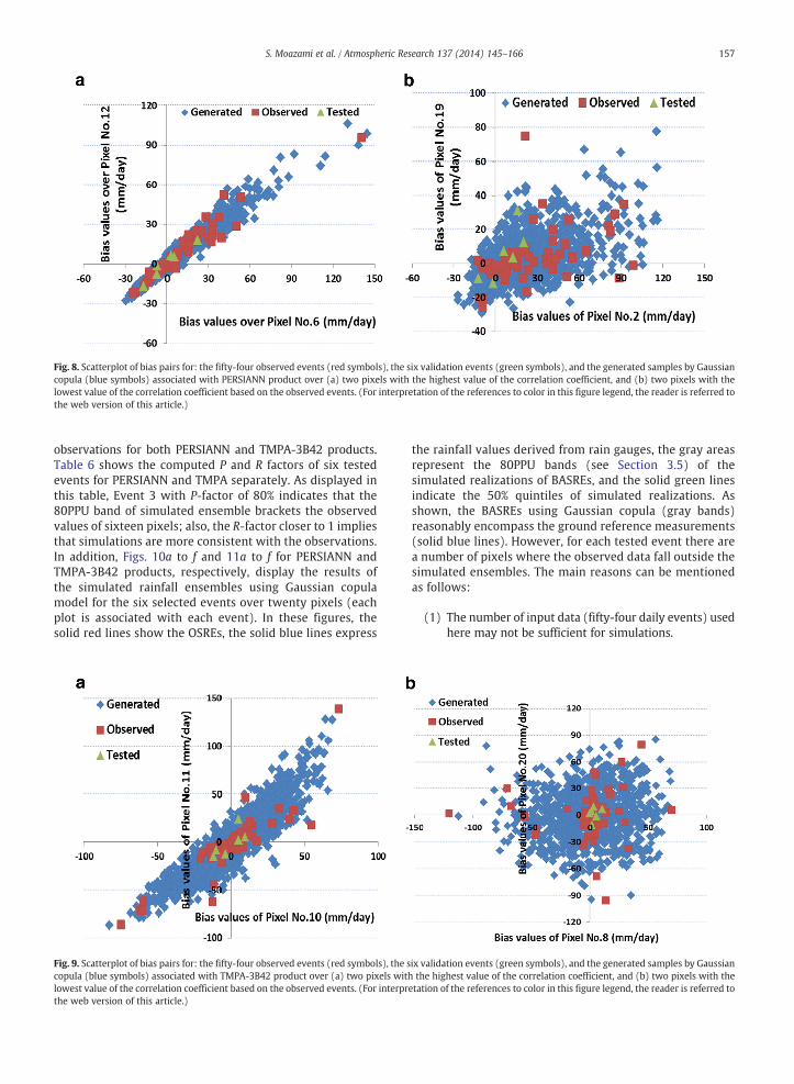
Fig. 8. Scatterplot of bias pairs for: the fifty-four observed events (red symbols), the six validation events (green symbols), and the generated samples by Gaussiancopula (blue symbols) associated with PERSIANN product over (a) two pixels with the highest value of the correlation coefficient, and (b) two pixels with thelowest value of the correlation coefficient based on the observed events. (For interpretation of the references to color in this figure legend, the reader is referred tothe web version of this article.)

157S. Moazami et al. / Atmospheric Research 137 (2014) 145–166

observations for both PERSIANN and TMPA-3B42 products.Table 6 shows the computed P and R factors of six testedevents for PERSIANN and TMPA separately. As displayed inthis table, Event 3 with P-factor of 80% indicates that the80PPU band of simulated ensemble brackets the observedvalues of sixteen pixels; also, the R-factor closer to 1 impliesthat simulations are more consistent with the observations.In addition, Figs. 10a to f and 11a to f for PERSIANN andTMPA-3B42 products, respectively, display the results ofthe simulated rainfall ensembles using Gaussian copulamodel for the six selected events over twenty pixels (eachplot is associated with each event). In these figures, thesolid red lines show the OSREs, the solid blue lines express

Fig. 9. Scatterplot of bias pairs for: the fifty-four observed events (red symbols), the scopula (blue symbols) associated with TMPA-3B42 product over (a) two pixels withlowest value of the correlation coefficient based on the observed events. (For interprthe web version of this article.)

the rainfall values derived from rain gauges, the gray areasrepresent the 80PPU bands (see Section 3.5) of thesimulated realizations of BASREs, and the solid green linesindicate the 50% quintiles of simulated realizations. Asshown, the BASREs using Gaussian copula (gray bands)reasonably encompass the ground reference measurements(solid blue lines). However, for each tested event there area number of pixels where the observed data fall outside thesimulated ensembles. The main reasons can be mentionedas follows:

(1) The number of input data (fifty-four daily events) usedhere may not be sufficient for simulations.

ix validation events (green symbols), and the generated samples by Gaussianthe highest value of the correlation coefficient, and (b) two pixels with the

etation of the references to color in this figure legend, the reader is referred to

Table 2Results of the average values of statistical indices of the six tested eventsover each pixel, comparison between the OSRE and BASRE (the 50% quantileof simulated realizations) for PERSIANN product.

Results of tested events (PERSIANN)

Pixel. no RMSE(BASRE) RMSE(OSRE) CC(BASRE) CC(OSRE)

1 7.59 14.10 0.82 0.242 8.93 11.87 0.19 0.343 2.57 7.68 0.87 0.284 1.93 6.48 0.86 0.335 1.79 9.04 0.93 0.166 5.34 8.32 0.93 0.477 6.09 10.71 0.69 0.418 3.83 5.07 0.42 0.729 3.50 6.59 −0.13 0.5610 1.75 7.24 0.83 0.2911 4.43 6.31 0.70 0.4412 5.64 9.80 0.32 −0.0613 7.01 9.72 0.37 0.1714 6.69 6.65 −0.16 −0.1015 1.30 8.52 0.95 0.1316 2.93 6.68 0.84 0.5417 8.15 3.62 0.56 0.9218 10.30 8.97 0.66 0.7919 7.64 6.56 0.43 0.7120 5.63 4.78 0.10 0.69Average 5.15 7.94 0.56 0.40

158 S. Moazami et al. / Atmospheric Research 137 (2014) 145–166

(2) Input data are associated with two different seasons(winter and spring) which may lead to different typesof storms.

(3) The quality assurance procedure employed on raingauge data may also have played a role.

Therefore, to improve the simulation, one can implementthe developed model by using a more reliable dataset of

Table 3Results of the average values of statistical indices of the six tested eventsover each pixel, comparison between the OSRE and BASRE (the 50% quantileof simulated realizations) for TMPA-3B42 product.

Results of tested events (TMPA-3B42)

Pixel. no RMSE(BASRE) RMSE(OSRE) CC(BASRE) CC(OSRE)

1 6.10 9.45 0.85 0.382 4.68 12.17 0.95 0.843 3.07 3.84 0.79 0.344 2.19 6.21 0.93 0.485 1.44 5.81 0.97 0.216 1.68 9.96 0.99 0.937 7.18 20.47 0.74 0.248 5.44 6.66 0.16 −0.329 4.42 6.65 −0.60 −0.2510 2.86 6.47 0.67 0.1211 2.43 7.46 0.89 0.6612 5.28 14.58 0.88 0.7513 6.50 15.57 0.42 0.2314 7.97 8.25 0.72 0.5115 1.46 3.58 0.94 0.4416 2.18 9.10 0.93 0.6517 2.14 5.33 0.98 0.8518 6.11 9.81 0.93 0.6819 7.15 7.10 0.68 0.7620 5.92 6.30 0.78 0.56Average 4.31 8.74 0.73 0.45

similar types of the rainfall observations at a fine temporalresolution (e.g. sub-daily) as input data.

5. Conclusions and recommendations

Reliable estimates of precipitation are essential forhydrologic applications and water resources planning, sinceuncertainties of precipitation as a major input data canpropagate into hydrological and meteorological models.Furthermore, detailed information of rainfall and a betterunderstanding of its spatial and temporal distributions areimportantly needed for predicting the available waterresources and optimal planning to use them effectively. Infact, precipitation is a key component of the global hydro-logical cycle; also, understanding the underlying processes inthe hydrological cycle is fundamental to water resourcesmanagement and climate studies. Therefore, satellite-basedprecipitation-estimate techniques which provide extendedprecipitation coverage beyond ground in situ data areincreasingly applied to atmospheric and hydrological appli-cations at different space-time scales (Hong et al., 2006a,b).Nevertheless, satellite-retrieved precipitations are less directthan ground-based data and lead to uncertainty in estimates.

In this study, the uncertainties associated with two highresolution satellite precipitation products (PERSIANN andTMPA-3B42) were described and adjusted through copula-based model. Since it is well known that rainfall data aredependent in both space and time, similar spatial structurebetween generations and observation fields can be animportant feature of rainfall simulation models. Therefore, acopula-based model that preserves the spatial dependencyamong variables independent of their marginal would be auseful method in the simulation of multivariate randomfields. Here, a multivariate Gaussian copula was developed inorder to simulate ensembles of bias-adjusted rainfall realiza-tions of SREs. In order to measure the robustness of thesimulated realizations of BASREs, two factors (P and R) werecomputed for each simulated ensemble by comparing it withthe observed data. In fact, using P and R, one can predict theuncertainty associated with the BASREs quantitatively. Fur-thermore, since each set of randomly generated biasesresulted in an individual pair of P and R factors for simulatedensemble, several sets of bias fieldswere generated randomly,a more appropriate set then was selected based on a betterpairs of P and R values. This procedure can lead to a moreaccurate simulation of ensembles. With respect to the threestatistical indices (Bias, RMSE, and CC) employed to evaluatethe performance of the bias-adjusted realizations, one canargue that the developed model was able to improve thesatellite rainfall estimates considerably. In addition, thevalidation results implied that the bias-adjusted band of thesimulated realizations encompassed the observed datareasonably.

It is worth remembering that the uncertainty analysisframework presented here was based on the simulatedensembles of bias fields. In future research, it would beinteresting to see how the technique reproduces the fulldistribution of bias using additional measures of reliability ofthe simulated ensembles. Various methods for the evaluationof ensemble-based forecasts can be found in the reviewby Tothet al. (2003). Moreover, using ensemble analysis instead of a

Table 4Results of Bias of the six tested events over each pixel, comparison between the OSRE and BASRE (the 50% quantile of simulated realizations) for PERSIANNproduct.

Bias of tested events (PERSIANN)

Event 1 Event 2 Event 3 Event 4 Event 5 Event 6

Pixel no Bias(OSRE)

Bias(BASRE)

Bias(OSRE)

Bias(BASRE)

Bias(OSRE)

Bias(BASRE)

Bias(OSRE)

Bias(BASRE)

Bias(OSRE)

Bias(BASRE)

Bias(OSRE)

Bias(BASRE)

1 13.4 2.5 −3.3 −1.5 −5.8 −1.5 −8.4 −9.9 25.6 14.5 −16.1 −2.72 7.3 −6.3 12.7 12.2 13.8 16.2 6.2 −1.6 16.0 −2.0 −12.2 −2.43 10.0 −1.8 −0.4 3.0 −3.1 1.4 7.1 2.5 17.0 3.2 −13.2 0.04 7.9 −1.5 −3.6 0.6 −7.4 −2.8 1.9 −1.3 13.2 3.0 −9.9 1.05 8.0 0.0 −6.7 −2.5 −4.5 0.8 −0.3 −1.5 12.3 1.2 −15.9 −0.96 8.2 3.0 −7.2 −2.3 −7.7 0.0 2.7 −1.9 21.9 11.8 −14.5 −0.67 3.5 −0.5 −6.6 −2.5 −17.6 −8.5 8.1 2.3 24.3 12.0 −15.8 −2.08 10.6 3.8 −5.0 −0.5 −7.5 −1.2 3.7 1.1 1.7 −8.2 −6.7 2.99 3.1 −2.1 −6.2 2.0 −5.3 2.1 5.4 2.2 1.8 −7.3 −10.2 2.310 4.9 2.0 −7.8 −1.6 −7.2 0.4 4.3 1.7 5.3 −3.6 −11.5 0.611 4.0 0.7 0.8 4.4 −11.6 −2.3 4.0 1.5 17.5 8.9 −8.4 2.912 4.5 6.8 −1.3 1.3 −8.2 0.2 6.5 −6.7 11.1 −6.0 −16.5 −6.113 3.0 −3.0 2.9 4.5 −8.7 −1.3 21.4 15.6 17.5 2.3 −12.2 −1.214 2.7 10.3 4.9 9.4 −7.9 4.5 5.4 0.8 11.5 −3.7 −10.3 −1.715 1.5 −0.3 −3.0 0.4 −8.3 −0.7 1.3 −2.8 10.0 −0.3 −14.3 −1.816 1.1 −0.9 0.6 2.2 −2.3 5.5 4.0 −0.8 13.0 3.7 −14.0 −1.317 −2.5 −8.6 −0.9 −0.5 −6.2 1.8 2.4 −2.0 31.8 16.6 0.4 4.218 7.0 −1.5 4.0 2.6 −8.7 −5.0 7.0 1.7 38.8 24.3 1.5 2.419 −4.0 −4.5 3.5 3.8 −11.2 −2.6 7.2 3.0 25.5 15.7 −7.2 −0.320 2.4 5.0 3.1 3.2 −5.6 2.4 7.4 −1.8 12.8 −5.0 1.9 −10.8Average 4.8 0.2 −1.0 1.9 −6.6 0.5 4.9 0.1 16.4 4.1 −10.2 −0.8

159S. Moazami et al. / Atmospheric Research 137 (2014) 145–166

single realization, one can improve the uncertainty assessmentof the error propagation from the precipitation input into thehydrological models and water resources simulations. Also,with respect to the extremeprecipitation events, i.e., floods anddroughts, using ensemble-based models, one can evaluate

Table 5Results of Bias of the six tested events over each pixel, comparison between the Oproduct.

Bias of tested events (TMPA-3B42)

Event 1 Event 2 Event 3

Pixel no Bias(OSRE)

Bias(BASRE)

Bias(OSRE)

Bias(BASRE)

Bias(OSRE)

Bias(BASRE)

1 −6.6 −0.5 0.4 0.2 −0.6 1.02 11.9 −0.2 −20.3 −7.7 −10.1 −2.93 4.6 −1.5 1.9 5.9 −2.0 0.84 9.4 −0.2 1.5 0.1 2.7 −3.85 7.8 −1.2 −2.4 −1.9 −9.4 −2.06 −13.5 −2.0 −7.3 −1.9 −15.4 −1.37 −1.7 −3.5 −35.1 −7.2 −32.3 −13.08 13.9 3.0 0.1 −1.9 4.8 −1.49 7.3 −1.9 3.7 2.7 7.8 1.610 8.2 0.4 −12.1 −2.0 4.1 −0.511 −0.2 −2.5 −15.0 0.8 −7.8 −5.112 −23.8 5.1 −6.1 6.0 −21.2 6.313 −5.6 −5.0 −3.7 5.0 −26.4 −3.614 −7.2 6.5 −3.0 11.5 −14.4 9.215 5.9 1.0 −0.6 −0.4 2.8 0.016 −7.8 −0.7 −0.7 0.6 −19.4 −0.717 3.2 −2.0 −1.2 0.0 −11.0 0.518 4.4 −0.2 4.0 4.0 −11.3 −3.619 3.0 −0.5 4.3 2.4 −1.0 1.220 0.7 1.8 1.8 7.0 −9.8 7.7Average 0.7 −0.2 −4.5 1.2 −8.5 −0.5

extreme prediction uncertainty and its associated risks for aspecified precipitation.

In this study as a first attempt to quantify and adjust theuncertainty associated with two major satellite-based pre-cipitation products over a developing region in Iran, a simple

SRE and BASRE (the 50% quantile of simulated realizations) for TMPA-3B42

Event 4 Event 5 Event 6

Bias(OSRE)

Bias(BASRE)

Bias(OSRE)

Bias(BASRE)

Bias(OSRE)

Bias(BASRE)

−9.9 −6.5 16.4 12.9 −12.0 −0.45.8 −1.0 12.8 0.0 5.9 6.3

−1.4 3.5 11.4 2.2 −7.2 1.4−0.8 −2.0 13.7 −1.0 −10.7 −0.9

2.0 −2.1 11.8 −1.8 −6.5 −0.90.3 −2.1 −10.7 −2.5 −2.5 2.1

−0.8 0.1 8.6 −0.3 −2.0 −0.13.5 −0.8 1.6 −12.8 5.9 0.96.4 3.1 2.0 −11.9 −9.6 −0.15.0 0.8 5.0 −8.8 −5.9 −1.42.4 −0.4 18.9 3.5 −2.0 2.35.2 7.5 −13.5 3.4 −3.7 1.5

13.6 14.5 13.4 −0.8 3.9 −0.92.2 9.0 11.2 4.0 3.3 5.1

−0.2 −2.6 10.2 −1.1 −5.9 −1.13.5 −1.0 7.0 0.5 −0.6 0.02.2 −0.8 4.9 3.3 3.1 0.94.9 3.2 19.7 13.3 1.7 −0.87.4 3.4 24.4 15.7 −1.2 −1.99.6 9.7 2.1 2.7 1.2 2.53.0 1.8 8.5 1.0 −2.2 0.7

Table 6Results of the P and R-factors of the six tested events for both PERSIANN and TMPA-3B42 products.

Satellite products PERSIANN TMPA-3B42

Tested events Event 1 Event 2 Event 3 Event 4 Event 5 Event 6 Event 1 Event 2 Event 3 Event 4 Event 5 Event 6

P-factor 65% 65% 80% 75% 50% 65% 80% 70% 80% 70% 70% 70%R-factor 2.16 1.28 1.14 1.35 1.07 1.59 1.94 1.57 1.12 1.22 0.98 1.22

Fig. 10. Comparison between original PERSIANN rainfall estimates (red line), rain gauge observations (blue line), and 80% confidence band associated withbias-adjusted rainfall estimates (gray band) of the six tested daily events (a, b, c, d, e, f) over twenty studied pixels (vertical and horizontal axes represent therainfall value (mm/day) and the number of pixel, respectively). (For interpretation of the references to color in this figure legend, the reader is referred to the webversion of this article.)

160 S. Moazami et al. / Atmospheric Research 137 (2014) 145–166

Fig. 11. Comparison between original TMPA-3B42 rainfall estimates (red line), rain gauge observations (blue line), and 80% confidence band associated withbias-adjusted rainfall estimates (gray band) of the six tested daily events (a, b, c, d, e, f) over twenty studied pixels (vertical and horizontal axes represent therainfall value (mm/day) and the number of pixel, respectively). (For interpretation of the references to color in this figure legend, the reader is referred to the webversion of this article.)

161S. Moazami et al. / Atmospheric Research 137 (2014) 145–166

copula (Gaussian) was selected to simulations. However, forfuture research, one can implement the method presentedhere using t-copula as another elliptical copula.

Themodel proposed herewas subject to various limitationssuch as unevenly distributed rain gauges over the study area.

Indeed, 50% of the selected pixels contained one rain gauge thatmay be inadequate to have an accurate simulation. However,to alleviate the effect of gauge uncertainties, pixels with aminimum of three rain gauges are required (Habib et al.,2009). Additionally, unreliable surface gauge measurements

Table A1Parametric distributions at each pixel for PERSIANN product.

Pixel no Distribution Parameter values

1 GEV k = −0.098 σ = 14.83 μ = 1.92 GEV 0.06 21.7 11.163 Logistic 11.46 12.814 Normal 19.9 8.175 GEV −0.027 14.01 −0.316 GEV 0.14 14.87 −0.5777 GEV 0.145 16.03 1.348 Normal 16.24 5.929 Logistic 8.85 5.4110 GEV 0.09 11.27 −1.02911 Logistic 13.1 8.112 GEV 0.084 13.5 −0.24713 Normal 22.98 14.7514 Normal 22.97 17.9115 GEV 0.184 11.44 −3.0416 Logistic 7.72 5.0717 GEV 0.176 15.75 3.18318 Normal 25.44 19.419 Normal 15.33 3.9120 GEV 0.243 12.32 −1.43

Table A2Parametric distributions at each pixel for TMPA-3B42 product.

Pixel no Distribution Parameter values

1 GEV k = −0.59 σ = 23.9 μ = −4.462 Normal 23 16.53 GEV −0.53 27.4 −4.434 Normal 30.03 −1.025 GEV −0.7 26.7 −3.156 GEV −0.4 32.16 −11.267 GEV −0.65 37.3 −9.048 GEV −0.71 26.9 −4.19 GEV −0.45 19.8 −3.0810 Logistic 13.87 1.0611 GEV −0.42 28.02 −8.512 Logistic 12.46 −0.11613 Logistic 18.99 −0.80514 GEV −0.65 31.6 −0.6615 GEV −0.31 18.3 −4.9116 Normal 23.74 −1.9617 Logistic 15.37 4.7418 GEV −0.28 22.2 2.619 GEV −0.14 14.6 −2.820 Normal 27.14 1.72

162 S. Moazami et al. / Atmospheric Research 137 (2014) 145–166

would result in erroneous parameter estimation, andconsequently unrealistic ensembles of uncertainty fields.Therefore, to verify the appropriateness of the presentedmodel, further investigations including simulations overregions with a dense rain gauge network, as well as in a finetemporal resolution (e.g. sub-daily) are required. Also, thepresented approach in this paper cannot be applied directlyto ungauged pixels without ground truth. In this case, thebias (observed or generated) could be extrapolated overungauged pixels using geostatistical techniques, e.g. InverseDistance Weighted (IDW) and Kriging (Shrestha, 2011).

Overall, the obtained results of this study indicated thatthe presented framework was able to adjust the uncertaintyassociated with the satellite precipitation products consid-erably. Moreover, the simulated biases and uncertaintybands here can be generalized over the ungauged basinswhere suffer from a lack of ground-based rainfall measure-ments considering the similarities in topography, physiog-raphy and climate conditions.

Acknowledgments

The authors would like to thank the two anonymousreviewers whose comments helped to improve the presen-tation significantly.

Appendix A. Probability distribution function of SREs bias

The fitted probability distribution function of fifty-fourobserved biases at each pixel is shown for PERSIANN andTMPA-3B42 products, respectively in Tables A1 and A2.Also, the related values of parameters for each marginaldistribution are presented in these tables. Note that “GEV”in Tables A1 and A2 refers to Generalized Extreme Valuedistribution. The GEV distribution is a flexible three-parameter model that combines the Gumbel, Fréchet, andWeibull maximum extreme value distributions. It has thefollowing PDF:

fx ¼1σ

exp − 1þ kzð Þ−1=k� �

1þ kzð Þ−1−1=k k≠1σ

exp −z− exp −zð Þð Þ k ¼ 0

8><>: ðA1Þ

Where z = (x − μ)/σ, x is the variable (here the value ofbias), and k, σ, μ are the shape, scale, and location parametersrespectively. The scale must be positive (sigma N 0), theshape and location can take on any real value. The range ofdefinition of the GEV distribution depends on k:

1þ kx−μð Þσ

N0 for k≠0

−∞ b x b þ ∞ for k ¼ 0ðA2Þ

Various values of the shape parameter yield the extremevalue type I, II, and III distributions. Specifically, the threecases k = 0, k N 0, and k b 0 correspond, respectively, to the

Gumbel, Fréchet, and Weibull families (Kotz and Nadarajah,2000).

Appendix B. Correlation coefficient of SREs bias

In this section the CC values of SREs bias between eachpair of twenty pixels are presented for both PERSIANN andTMPA-3B42 products, respectively in Tables B1 and B2. Inthese tables, “Obs”, “Gen”, and “Tes”, respectively, refer to thefifty-four observed, one thousand generated, and six testedevents. As shown the randomly generated biases retain thecorrelation imposed in the copula model which was derivedfrom the observed values.

Table B1The CC values of the bias between each pair of twenty pixels for PERSIANN product based on the fifty-four observed (Obs), one thousand generated (Gen), and sixtested (Tes) events.

Event Pixel 1 2 3 4 5 6 7 8 9 10 11 12 13 14 15 16 17 18 19 20

Obs 1 1.00 0.76 0.85 0.80 0.86 0.77 0.69 0.77 0.77 0.79 0.71 0.79 0.72 0.60 0.76 0.82 0.52 0.55 0.52 0.48Gen 1.00 0.75 0.87 0.85 0.88 0.83 0.68 0.78 0.77 0.82 0.78 0.82 0.71 0.63 0.79 0.82 0.59 0.55 0.65 0.57Tes 1.00 0.83 0.90 0.92 0.93 0.87 0.75 0.66 0.69 0.78 0.84 0.82 0.33 0.76 0.82 0.64 0.74 0.79 0.81 0.57Obs 2 0.76 1.00 0.82 0.75 0.76 0.65 0.70 0.68 0.69 0.65 0.64 0.72 0.78 0.73 0.64 0.71 0.64 0.62 0.43 0.58Gen 0.75 1.00 0.78 0.70 0.71 0.68 0.63 0.62 0.61 0.64 0.62 0.70 0.76 0.77 0.63 0.68 0.70 0.59 0.49 0.64Tes 0.83 1.00 0.90 0.83 0.84 0.74 0.67 0.70 0.80 0.83 0.81 0.83 0.62 0.79 0.91 0.88 0.63 0.64 0.78 0.66Obs 3 0.85 0.82 1.00 0.92 0.93 0.79 0.73 0.79 0.85 0.84 0.77 0.86 0.80 0.66 0.84 0.76 0.59 0.68 0.57 0.65Gen 0.87 0.78 1.00 0.93 0.94 0.86 0.76 0.82 0.85 0.87 0.85 0.89 0.82 0.73 0.88 0.80 0.72 0.70 0.71 0.71Tes 0.90 0.90 1.00 0.95 0.97 0.90 0.83 0.86 0.92 0.97 0.87 0.92 0.65 0.81 0.95 0.83 0.74 0.75 0.85 0.71Obs 4 0.80 0.75 0.92 1.00 0.92 0.88 0.74 0.87 0.91 0.92 0.90 0.93 0.83 0.61 0.89 0.79 0.56 0.70 0.62 0.67Gen 0.85 0.70 0.93 1.00 0.95 0.89 0.74 0.87 0.91 0.93 0.92 0.92 0.79 0.67 0.91 0.81 0.66 0.67 0.75 0.69Tes 0.92 0.83 0.95 1.00 1.00 0.95 0.88 0.72 0.83 0.89 0.91 0.94 0.63 0.85 0.92 0.81 0.66 0.76 0.84 0.63Obs 5 0.86 0.76 0.93 0.92 1.00 0.83 0.71 0.85 0.90 0.91 0.81 0.88 0.77 0.61 0.85 0.79 0.58 0.66 0.60 0.66Gen 0.88 0.71 0.94 0.95 1.00 0.89 0.75 0.87 0.91 0.94 0.90 0.91 0.77 0.66 0.90 0.81 0.67 0.66 0.74 0.70Tes 0.93 0.84 0.97 1.00 1.00 0.93 0.85 0.78 0.86 0.91 0.88 0.92 0.60 0.81 0.91 0.79 0.66 0.73 0.81 0.60Obs 6 0.77 0.65 0.79 0.88 0.83 1.00 0.72 0.87 0.82 0.90 0.93 0.96 0.80 0.53 0.81 0.80 0.55 0.62 0.60 0.52Gen 0.83 0.68 0.86 0.89 0.89 1.00 0.82 0.89 0.85 0.91 0.92 0.97 0.78 0.65 0.85 0.80 0.71 0.66 0.75 0.70Tes 0.87 0.74 0.90 0.95 0.93 1.00 0.97 0.61 0.72 0.83 0.97 0.97 0.63 0.92 0.92 0.80 0.81 0.90 0.94 0.79Obs 7 0.69 0.70 0.73 0.74 0.71 0.72 1.00 0.83 0.71 0.72 0.70 0.78 0.83 0.72 0.68 0.66 0.73 0.70 0.49 0.67Gen 0.68 0.63 0.76 0.74 0.75 0.82 1.00 0.83 0.73 0.78 0.76 0.82 0.80 0.73 0.72 0.67 0.83 0.75 0.62 0.78Tes 0.75 0.67 0.83 0.88 0.85 0.97 1.00 0.53 0.67 0.79 0.97 0.97 0.72 0.94 0.90 0.83 0.80 0.90 0.94 0.86Obs 8 0.77 0.68 0.79 0.87 0.85 0.87 0.83 1.00 0.88 0.89 0.84 0.90 0.83 0.63 0.78 0.79 0.68 0.71 0.63 0.66Gen 0.78 0.62 0.82 0.87 0.87 0.89 0.83 1.00 0.88 0.90 0.88 0.91 0.78 0.69 0.83 0.78 0.74 0.71 0.75 0.71Tes 0.66 0.70 0.86 0.72 0.78 0.61 0.53 1.00 0.95 0.93 0.51 0.62 0.52 0.41 0.71 0.58 0.49 0.40 0.51 0.43Obs 9 0.77 0.69 0.85 0.91 0.90 0.82 0.71 0.88 1.00 0.93 0.80 0.87 0.76 0.60 0.76 0.74 0.60 0.73 0.58 0.64Gen 0.77 0.61 0.85 0.91 0.91 0.85 0.73 0.88 1.00 0.95 0.84 0.87 0.72 0.64 0.82 0.73 0.66 0.70 0.74 0.67Tes 0.69 0.80 0.92 0.83 0.86 0.72 0.67 0.95 1.00 0.98 0.67 0.78 0.74 0.60 0.85 0.79 0.48 0.46 0.62 0.53Obs 10 0.79 0.65 0.84 0.92 0.91 0.90 0.72 0.89 0.93 1.00 0.91 0.93 0.80 0.57 0.89 0.77 0.58 0.70 0.61 0.65Gen 0.82 0.64 0.87 0.93 0.94 0.91 0.78 0.90 0.95 1.00 0.92 0.92 0.76 0.65 0.90 0.76 0.68 0.72 0.74 0.70Tes 0.78 0.83 0.97 0.89 0.91 0.83 0.79 0.93 0.98 1.00 0.78 0.87 0.73 0.71 0.91 0.82 0.64 0.63 0.76 0.66Obs 11 0.71 0.64 0.77 0.90 0.81 0.93 0.70 0.84 0.80 0.91 1.00 0.94 0.82 0.50 0.88 0.78 0.50 0.61 0.59 0.54Gen 0.78 0.62 0.85 0.92 0.90 0.92 0.76 0.88 0.84 0.92 1.00 0.94 0.79 0.65 0.92 0.80 0.66 0.64 0.74 0.65Tes 0.84 0.81 0.87 0.91 0.88 0.97 0.97 0.51 0.67 0.78 1.00 0.98 0.68 0.99 0.95 0.87 0.81 0.91 0.97 0.85Obs 12 0.79 0.72 0.86 0.93 0.88 0.96 0.78 0.90 0.87 0.93 0.94 1.00 0.84 0.62 0.86 0.82 0.61 0.68 0.69 0.64Gen 0.82 0.70 0.89 0.92 0.91 0.97 0.82 0.91 0.87 0.92 0.94 1.00 0.81 0.70 0.88 0.83 0.74 0.68 0.80 0.72Tes 0.82 0.83 0.92 0.94 0.92 0.97 0.97 0.62 0.78 0.87 0.98 1.00 0.78 0.96 0.98 0.92 0.76 0.85 0.94 0.83Obs 13 0.72 0.78 0.80 0.83 0.77 0.80 0.83 0.83 0.76 0.80 0.82 0.84 1.00 0.78 0.75 0.78 0.80 0.78 0.56 0.72Gen 0.71 0.76 0.82 0.79 0.77 0.78 0.80 0.78 0.72 0.76 0.79 0.81 1.00 0.85 0.79 0.75 0.88 0.77 0.65 0.81Tes 0.33 0.62 0.65 0.63 0.60 0.63 0.72 0.52 0.74 0.73 0.68 0.78 1.00 0.71 0.80 0.90 0.34 0.42 0.61 0.65Obs 14 0.60 0.73 0.66 0.61 0.61 0.53 0.72 0.63 0.60 0.57 0.50 0.62 0.78 1.00 0.55 0.63 0.82 0.75 0.44 0.64Gen 0.63 0.77 0.73 0.67 0.66 0.65 0.73 0.69 0.64 0.65 0.65 0.70 0.85 1.00 0.65 0.66 0.87 0.80 0.53 0.71Tes 0.76 0.79 0.81 0.85 0.81 0.92 0.94 0.41 0.60 0.71 0.99 0.96 0.71 1.00 0.93 0.90 0.76 0.88 0.95 0.85Obs 15 0.76 0.64 0.84 0.89 0.85 0.81 0.68 0.78 0.76 0.89 0.88 0.86 0.75 0.55 1.00 0.74 0.49 0.60 0.63 0.66Gen 0.79 0.63 0.88 0.91 0.90 0.85 0.72 0.83 0.82 0.90 0.92 0.88 0.79 0.65 1.00 0.80 0.64 0.63 0.78 0.69Tes 0.82 0.91 0.95 0.92 0.91 0.92 0.90 0.71 0.85 0.91 0.95 0.98 0.80 0.93 1.00 0.95 0.74 0.79 0.92 0.82Obs 16 0.82 0.71 0.76 0.79 0.79 0.80 0.66 0.79 0.74 0.77 0.78 0.82 0.78 0.63 0.74 1.00 0.65 0.58 0.62 0.50Gen 0.82 0.68 0.80 0.81 0.81 0.80 0.67 0.78 0.73 0.76 0.80 0.83 0.75 0.66 0.80 1.00 0.69 0.55 0.75 0.62Tes 0.64 0.88 0.83 0.81 0.79 0.80 0.83 0.58 0.79 0.82 0.87 0.92 0.90 0.90 0.95 1.00 0.57 0.65 0.82 0.77Obs 17 0.52 0.64 0.59 0.56 0.58 0.55 0.73 0.68 0.60 0.58 0.50 0.61 0.80 0.82 0.49 0.65 1.00 0.87 0.51 0.81Gen 0.59 0.70 0.72 0.66 0.67 0.71 0.83 0.74 0.66 0.68 0.66 0.74 0.88 0.87 0.64 0.69 1.00 0.87 0.59 0.88Tes 0.74 0.63 0.74 0.66 0.66 0.81 0.80 0.49 0.48 0.64 0.81 0.76 0.34 0.76 0.74 0.57 1.00 0.96 0.92 0.90Obs 18 0.55 0.62 0.68 0.70 0.66 0.62 0.70 0.71 0.73 0.70 0.61 0.68 0.78 0.75 0.60 0.58 0.87 1.00 0.49 0.81Gen 0.55 0.59 0.70 0.67 0.66 0.66 0.75 0.71 0.70 0.72 0.64 0.68 0.77 0.80 0.63 0.55 0.87 1.00 0.50 0.78Tes 0.79 0.64 0.75 0.76 0.73 0.90 0.90 0.40 0.46 0.63 0.91 0.85 0.42 0.88 0.79 0.65 0.96 1.00 0.97 0.90Obs 19 0.52 0.43 0.57 0.62 0.60 0.60 0.49 0.63 0.58 0.61 0.59 0.69 0.56 0.44 0.63 0.62 0.51 0.49 1.00 0.50Gen 0.65 0.49 0.71 0.75 0.74 0.75 0.62 0.75 0.74 0.74 0.74 0.80 0.65 0.53 0.78 0.75 0.59 0.50 1.00 0.57Tes 0.81 0.78 0.85 0.84 0.81 0.94 0.94 0.51 0.62 0.76 0.97 0.94 0.61 0.95 0.92 0.82 0.92 0.97 1.00 0.93Obs 20 0.48 0.58 0.65 0.67 0.66 0.52 0.67 0.66 0.64 0.65 0.54 0.64 0.72 0.64 0.66 0.50 0.81 0.81 0.50 1.00Gen 0.57 0.64 0.71 0.69 0.70 0.70 0.78 0.71 0.67 0.70 0.65 0.72 0.81 0.71 0.69 0.62 0.88 0.78 0.57 1.00Tes 0.57 0.66 0.71 0.63 0.60 0.79 0.86 0.43 0.53 0.66 0.85 0.83 0.65 0.85 0.82 0.77 0.90 0.90 0.93 1.00

163S. Moazami et al. / Atmospheric Research 137 (2014) 145–166

References

Abbaspour, K.C., Johnson, C.A., Van Genuchten, M. Th., 2004. Estimatinguncertain flow and transport parameters using a sequential uncertaintyfitting procedure. Vadose Zone J. 3, 1340–1352.

Abbaspour, K.C., Yang, J., Maximov, I., Siber, R., Bogner, K., Mieleitner, J.,Zobrist, J., Srinivasan, R., 2007. Spatiallydistributed modelling of

hydrology and water quality in the pre-alpine/alpine Thur watershedusing SWAT. J. Hydrol. 333, 413–430.

AghaKouchak, A., 2010. Simulation of Remotely Sensed Rainfall Fields UsingCopulas. Institut für Wasserbau der Universität Stuttgart.

AghaKouchak, A., Nasrollahi, N., Habib, E., 2009. Accounting for uncertainties ofthe TRMM satellite estimates. J. Remote Sens. 1, 606–619. http://dx.doi.org/10.3390/rs1030606.

Table B2The CC values of the bias between each pair of twenty pixels for TMPA-3B42 product based on the fifty-four observed (Obs), one thousand generated (Gen), andsix tested (Tes) events.

Event Pixel 1 2 3 4 5 6 7 8 9 10 11 12 13 14 15 16 17 18 19 20

Obs 1 1.00 0.33 0.65 0.62 0.51 0.45 0.41 0.56 0.43 0.36 0.42 0.42 0.41 0.20 0.38 0.34 0.33 0.20 0.27 0.43Gen 1.00 0.34 0.65 0.62 0.55 0.47 0.41 0.61 0.47 0.40 0.41 0.44 0.44 0.25 0.41 0.36 0.31 0.22 0.29 0.43Tes 1.00 0.36 0.98 0.75 0.84 0.51 0.34 0.34 0.58 0.59 0.69 0.53 0.39 0.74 0.90 0.57 0.74 0.91 0.84 0.60Obs 2 0.33 1.00 0.53 0.29 0.44 0.38 0.46 0.32 0.41 0.45 0.45 0.53 0.47 0.52 0.41 0.39 0.46 0.31 0.29 0.37Gen 0.34 1.00 0.57 0.28 0.46 0.36 0.43 0.35 0.40 0.44 0.42 0.51 0.44 0.52 0.42 0.35 0.45 0.30 0.23 0.37Tes 0.36 1.00 0.45 0.23 0.51 0.25 0.93 0.69 0.10 0.80 0.67 0.23 0.28 0.37 0.32 0.08 0.60 0.43 0.41 0.23Obs 3 0.65 0.53 1.00 0.69 0.78 0.61 0.47 0.49 0.49 0.52 0.57 0.62 0.41 0.38 0.59 0.49 0.45 0.30 0.37 0.54Gen 0.65 0.57 1.00 0.71 0.80 0.59 0.47 0.54 0.51 0.57 0.59 0.65 0.41 0.38 0.62 0.48 0.46 0.32 0.33 0.59Tes 0.98 0.45 1.00 0.75 0.85 0.53 0.38 0.46 0.66 0.69 0.66 0.52 0.37 0.64 0.87 0.53 0.79 0.85 0.77 0.59Obs 4 0.62 0.29 0.69 1.00 0.74 0.67 0.26 0.70 0.60 0.62 0.66 0.52 0.33 0.19 0.55 0.34 0.31 0.41 0.42 0.40Gen 0.62 0.28 0.71 1.00 0.76 0.66 0.26 0.72 0.60 0.64 0.63 0.50 0.31 0.21 0.54 0.36 0.26 0.42 0.41 0.44Tes 0.75 0.23 0.75 1.00 0.93 0.03 0.18 0.11 0.77 0.63 0.65 0.02 0.10 0.51 0.89 0.16 0.21 0.67 0.79 0.28Obs 5 0.51 0.44 0.78 0.74 1.00 0.69 0.40 0.50 0.57 0.74 0.69 0.73 0.41 0.39 0.72 0.64 0.44 0.37 0.50 0.46Gen 0.55 0.46 0.80 0.76 1.00 0.70 0.40 0.58 0.63 0.79 0.73 0.76 0.44 0.38 0.75 0.65 0.42 0.38 0.49 0.47Tes 0.84 0.51 0.85 0.93 1.00 0.23 0.50 0.15 0.73 0.83 0.85 0.29 0.38 0.69 0.96 0.37 0.48 0.83 0.90 0.51Obs 6 0.45 0.38 0.61 0.67 0.69 1.00 0.46 0.59 0.59 0.68 0.75 0.71 0.53 0.38 0.73 0.60 0.37 0.33 0.55 0.20Gen 0.47 0.36 0.59 0.66 0.70 1.00 0.44 0.64 0.60 0.68 0.73 0.70 0.51 0.38 0.71 0.63 0.32 0.31 0.55 0.19Tes 0.51 0.25 0.53 0.03 0.23 1.00 0.33 0.61 0.28 0.37 0.28 0.98 0.82 0.48 0.35 0.91 0.83 0.51 0.29 0.89Obs 7 0.41 0.46 0.47 0.26 0.40 0.46 1.00 0.23 0.30 0.34 0.41 0.58 0.79 0.74 0.31 0.64 0.80 0.52 0.35 0.57Gen 0.41 0.43 0.47 0.26 0.40 0.44 1.00 0.30 0.34 0.34 0.39 0.57 0.74 0.64 0.31 0.59 0.77 0.48 0.40 0.54Tes 0.34 0.93 0.38 0.18 0.50 0.33 1.00 0.51 0.02 0.73 0.80 0.36 0.50 0.60 0.38 0.27 0.56 0.56 0.54 0.39Obs 8 0.56 0.32 0.49 0.70 0.50 0.59 0.23 1.00 0.82 0.66 0.63 0.50 0.32 0.15 0.59 0.30 0.22 0.22 0.38 0.09Gen 0.61 0.35 0.54 0.72 0.58 0.64 0.30 1.00 0.83 0.69 0.65 0.54 0.36 0.21 0.58 0.39 0.25 0.28 0.44 0.16Tes 0.34 0.69 0.46 0.11 0.15 0.61 0.51 1.00 0.11 0.51 0.16 0.48 0.24 0.04 0.04 0.25 0.83 0.20 0.00 0.31Obs 9 0.43 0.41 0.49 0.60 0.57 0.59 0.30 0.82 1.00 0.77 0.69 0.69 0.44 0.35 0.64 0.41 0.32 0.34 0.46 0.15Gen 0.47 0.40 0.51 0.60 0.63 0.60 0.34 0.83 1.00 0.78 0.68 0.70 0.45 0.37 0.59 0.46 0.33 0.37 0.52 0.18Tes 0.58 0.10 0.66 0.77 0.73 0.28 0.02 0.11 1.00 0.65 0.31 0.27 0.30 0.19 0.69 0.34 0.30 0.39 0.45 0.50Obs 10 0.36 0.45 0.52 0.62 0.74 0.68 0.34 0.66 0.77 1.00 0.89 0.85 0.53 0.39 0.77 0.50 0.41 0.38 0.48 0.24Gen 0.40 0.44 0.57 0.64 0.79 0.68 0.34 0.69 0.78 1.00 0.91 0.85 0.51 0.40 0.76 0.54 0.40 0.38 0.48 0.27Tes 0.59 0.80 0.69 0.63 0.83 0.37 0.73 0.51 0.65 1.00 0.76 0.37 0.49 0.47 0.68 0.33 0.59 0.60 0.63 0.54Obs 11 0.42 0.45 0.57 0.66 0.69 0.75 0.41 0.63 0.69 0.89 1.00 0.89 0.57 0.42 0.76 0.62 0.41 0.35 0.49 0.19Gen 0.41 0.42 0.59 0.63 0.73 0.73 0.39 0.65 0.68 0.91 1.00 0.90 0.52 0.40 0.77 0.64 0.37 0.32 0.48 0.21Tes 0.69 0.67 0.66 0.65 0.85 0.28 0.80 0.16 0.31 0.76 1.00 0.38 0.54 0.88 0.83 0.43 0.49 0.88 0.93 0.54Obs 12 0.42 0.53 0.62 0.52 0.73 0.71 0.58 0.50 0.69 0.85 0.89 1.00 0.65 0.55 0.71 0.74 0.52 0.36 0.53 0.29Gen 0.44 0.51 0.65 0.50 0.76 0.70 0.57 0.54 0.70 0.85 0.90 1.00 0.64 0.51 0.73 0.75 0.49 0.34 0.52 0.30Tes 0.53 0.23 0.52 0.02 0.29 0.98 0.36 0.48 0.27 0.37 0.38 1.00 0.89 0.60 0.43 0.96 0.78 0.59 0.40 0.94Obs 13 0.41 0.47 0.41 0.33 0.41 0.53 0.79 0.32 0.44 0.53 0.57 0.65 1.00 0.79 0.52 0.53 0.76 0.54 0.29 0.47Gen 0.44 0.44 0.41 0.31 0.44 0.51 0.74 0.36 0.45 0.51 0.52 0.64 1.00 0.72 0.52 0.55 0.73 0.54 0.28 0.47Tes 0.39 0.28 0.37 0.10 0.38 0.82 0.50 0.24 0.30 0.49 0.54 0.89 1.00 0.67 0.48 0.91 0.55 0.58 0.49 0.95Obs 14 0.20 0.52 0.38 0.19 0.39 0.38 0.74 0.15 0.35 0.39 0.42 0.55 0.79 1.00 0.45 0.56 0.83 0.59 0.22 0.52Gen 0.25 0.52 0.38 0.21 0.38 0.38 0.64 0.21 0.37 0.40 0.40 0.51 0.72 1.00 0.43 0.49 0.80 0.58 0.25 0.48Tes 0.74 0.37 0.64 0.51 0.69 0.48 0.60 0.04 0.19 0.47 0.88 0.60 0.67 1.00 0.81 0.69 0.53 0.95 0.92 0.69Obs 15 0.38 0.41 0.59 0.55 0.72 0.73 0.31 0.59 0.64 0.77 0.76 0.71 0.52 0.45 1.00 0.57 0.46 0.37 0.53 0.28Gen 0.41 0.42 0.62 0.54 0.75 0.71 0.31 0.58 0.59 0.76 0.77 0.73 0.52 0.43 1.00 0.62 0.45 0.33 0.48 0.30Tes 0.90 0.32 0.87 0.89 0.96 0.35 0.38 0.04 0.69 0.68 0.83 0.43 0.48 0.81 1.00 0.55 0.49 0.91 0.95 0.63Obs 16 0.34 0.39 0.49 0.34 0.64 0.60 0.64 0.30 0.41 0.50 0.62 0.74 0.53 0.56 0.57 1.00 0.58 0.40 0.43 0.28Gen 0.36 0.35 0.48 0.36 0.65 0.63 0.59 0.39 0.46 0.54 0.64 0.75 0.55 0.49 0.62 1.00 0.52 0.38 0.47 0.23Tes 0.57 0.08 0.53 0.16 0.37 0.91 0.27 0.25 0.34 0.33 0.43 0.96 0.91 0.69 0.55 1.00 0.65 0.66 0.51 0.97Obs 17 0.33 0.46 0.45 0.31 0.44 0.37 0.80 0.22 0.32 0.41 0.41 0.52 0.76 0.83 0.46 0.58 1.00 0.75 0.33 0.67Gen 0.31 0.45 0.46 0.26 0.42 0.32 0.77 0.25 0.33 0.40 0.37 0.49 0.73 0.80 0.45 0.52 1.00 0.73 0.30 0.66Tes 0.74 0.60 0.79 0.21 0.48 0.83 0.56 0.83 0.30 0.59 0.49 0.78 0.55 0.53 0.49 0.65 1.00 0.67 0.46 0.68Obs 18 0.20 0.31 0.30 0.41 0.37 0.33 0.52 0.22 0.34 0.38 0.35 0.36 0.54 0.59 0.37 0.40 0.75 1.00 0.36 0.72Gen 0.22 0.30 0.32 0.42 0.38 0.31 0.48 0.28 0.37 0.38 0.32 0.34 0.54 0.58 0.33 0.38 0.73 1.00 0.36 0.71Tes 0.91 0.43 0.85 0.67 0.83 0.51 0.56 0.20 0.39 0.60 0.88 0.59 0.58 0.95 0.91 0.66 0.67 1.00 0.96 0.69Obs 19 0.27 0.29 0.37 0.42 0.50 0.55 0.35 0.38 0.46 0.48 0.49 0.53 0.29 0.22 0.53 0.43 0.33 0.36 1.00 0.31Gen 0.29 0.23 0.33 0.41 0.49 0.55 0.40 0.44 0.52 0.48 0.48 0.52 0.28 0.25 0.48 0.47 0.30 0.36 1.00 0.29Tes 0.84 0.41 0.77 0.79 0.90 0.29 0.54 0.00 0.45 0.63 0.93 0.40 0.49 0.92 0.95 0.51 0.46 0.96 1.00 0.57Obs 20 0.43 0.37 0.54 0.40 0.46 0.20 0.57 0.09 0.15 0.24 0.19 0.29 0.47 0.52 0.28 0.28 0.67 0.72 0.31 1.00Gen 0.43 0.37 0.59 0.44 0.47 0.19 0.54 0.16 0.18 0.27 0.21 0.30 0.47 0.48 0.30 0.23 0.66 0.71 0.29 1.00Tes 0.60 0.23 0.59 0.28 0.51 0.89 0.39 0.31 0.50 0.54 0.54 0.94 0.95 0.69 0.63 0.97 0.68 0.69 0.57 1.00

164 S. Moazami et al. / Atmospheric Research 137 (2014) 145–166

Aghakouchak, A., Habib, E., Bárdossy, A., 2010a. A comparison of threeremotely sensed rainfall ensemble generators. Atmos. Res. 02234,13.

AghaKouchak, A., Bárdossy, A., Habib, E., 2010b. Conditional simulation ofremotely sensed rainfall data using a non-Gaussian v-transformedcopula. Adv. Water Resour. 33, 624–634.

AghaKouchak, A., Bárdossy, A., Habib, E., 2010c. Copula-based uncertaintymodelling: application to multisensor precipitation estimates. Hydrol.Process. 24, 2111–2124. http://dx.doi.org/10.1002/hyp.7632.

AghaKouchak, A., Behrangi, A., Sorooshian, S., Hsu, K., Amitai, E., 2011. Evaluation ofsatellite‐retrieved extreme precipitation rates across the central United States.J. Geophys. Res. 116, D02115. http://dx.doi.org/10.1029/2010JD014741.

165S. Moazami et al. / Atmospheric Research 137 (2014) 145–166

AghaKouchak, A., Mehran, A., Norouzi, H., Behrangi, A., 2012. Systematic andrandom error components in satellite precipitation data sets. Geophys.Res. Lett. 39, L09406. http://dx.doi.org/10.1029/2012GL051592.

Behrangi, A., Khakbaz, B., JaW, T.C., AghaKouchak, A., Hsu, K., Sorooshian,S., 2011. Hydrologic evaluation of satellite precipitation products overa mid-size basin. J. Hydrol. 397, 225–237. http://dx.doi.org/10.1016/j.jhydrol.11.043.

Bellerby, T., Sun, J., 2005. Probabilistic and ensemble representations ofthe uncertainty in an IR/microwave satellite precipitation product.J. Hydrometeorol. 6, 1032–1044.

Ben-Gal, I., 2005. Outlier detection. In: Maimon, O., Rockach, L. (Eds.), DataMining and Knowledge Discovery Handbook: A Complete Guide forPractitioners and Researchers. Kluwer Academic Publishers. ISBN: 0-387-24435-2.

Bitew, M.M., Gebremichael, M., 2011. Evaluation of satellite rainfall productsthrough hydrologic simulation in a fully distributed hydrologic model.Water Resour. Res. 47, W06526. http://dx.doi.org/10.1029/WR009917.

Cherubini, U., Luciano, E., Vecchiato, W., 2004. Copula Methods in Finance.John Wiley & Sons Ltd., The Atrium, Southern Gate, Chichester,WestSussex PO19 8SQ, England0-470-86344-7.

Ciach, G.J., Krajewski, W.F., Villarini, G., 2007. Product-error-drivenuncertainty model for probabilistic quantitative precipitation estimationwith NEXRAD data. J. Hydrometeorol. 8, 1325–1347. http://dx.doi.org/10.1175/2007JHM814.1.

Di Baldassarre, G., Laio, F., Montanari, A., 2009. Design flood estimation usingmodel selection criteria. Phys. Chem. Earth 34 (10–12), 606–611.

Dinku, T., Connor, S.J., Ceccato, P., 2010. Comparison of CMORPH and TRMM-3B42 over mountainous regions of Africa and South America. In:Gebremichael, M., Hossaim, F. (Eds.), Satellite Rainfall Applications forSurface Hydrology. Springer Science+Business Media B.V., pp. 193–204.

Draper, N.R., Smith, H., 1998. Applied Regression Analysis, 3rd edition. WileySeries in Probability and Statistics (ISBN-13: 978-0471170822).

Ebert, E.E., Janowiak, J.E., Kidd, C., 2007. Comparison of near-real-timeprecipitation estimates from satellite observations and numerical models.Bull. Am. Meteorol. Soc. 88, 47–64. http://dx.doi.org/10.1175/BAMS-88-1-47.

Evin, G., Favre, A.C., 2008. A new rainfall model based on the Neyman–Scottprocess using cubic copulas. Water Resour. Res. 44, W03433. http://dx.doi.org/10.1029/2007WR006054.

Fang, Y., 2012. Extensions to Gaussian Copula Models (A dissertation submittedto Oregon State University in partial fulfillment of the requirements for thedegree of Doctor of Philosophy).

Favre, A.C., El Adlouni, S., Perreault, L., Thie'monge, N., Bobe'e, B., 2004.Multivariate hydrological frequency analysis using copulas. WaterResour. Res. W01101. http://dx.doi.org/10.1029/2003WR002456.

Filzmoser, P., 2005. A multivariate outlier detection method. Technical report.Department of Statistics and Probability Theory, Vienna, AUSTRIA.

Frahm, G., Junker, M., Schmidt, R., 2005. Estimating the tail-dependencecoefficient: properties and pitfalls. Insur. Math. Econ. 37, 80–100.

Gebremichael, M., Krajewski, W.F., Morrissey, M.L., Huffman, G.J., Adler, R.F.,2005. A detailed evaluation of GPCP one-degree daily rainfall estimatesover the Mississippi River Basin. J. Appl. Meteorol. 44 (5), 665–681.

Genest, C., Favre, A.-C., 2007. Everything you always wanted to know aboutcopula modeling but were afraid to ask. J. Hydrol. Eng. 12 (4), 347–368.

Germann, U., Berenguer, M., Sempere-Torres, D., Salvade, G., 2006. Ensembleradar precipitation — a new topic on the radar horizon. Proceeding ofthe 4th European Conference on Radar in Meteorology and HydrologyERAD, Barcelona, 18–22 September 2006.

Grimaldi, S., Serinaldi, F., 2006. Asymmetric copula in multivariate floodfrequency analysis. Adv. Water Resour. 29, 1155–1167.

Habib, E., Henschke, A., Adler, R., 2009. Evaluation of TMPA satellite-basedresearch and real-time rainfall estimates during six tropical-relatedheavy rainfall events over Louisiana, USA. Atmos. Res. http://dx.doi.org/10.1016/j.atmosres.2009.06.015.

Hirpa, F.A., Gebremichael, M., Hopson, T., 2010. Evaluation of high resolutionsatellite precipitation products over very complex terrain in Ethiopia.J. Appl. Meteorol. Climatol. 49, 1044–1051. http://dx.doi.org/10.1175/JAMC2298.1.

Hodge, V.J., and Austin, J., 2004. A Survey of Outlier Detection Methodolo-gies. Dept. of Computer Science, University of York, York, UK, KluwerAcademic Publishers.

Hong, Y., Adler, R., Huffman, G., 2006a. Evaluation of the potential of NASAmulti-satellite precipitation analysis in global landslide hazard assess-ment. Geophys. Res. Lett. 33, L22402. http://dx.doi.org/10.1029/GL028010.

Hong, Y., Hsu, K., Moradkhani, H., Sorooshian, S., 2006b. Uncertaintyquantification of satellite precipitation estimation and Monte Carloassessment of the error propagation into hydrologic response. WaterResour. Res. 42, W08421. http://dx.doi.org/10.1029/WR004398.

Hong, Y., Gochis, D., Cheng, J., Hsu, K., Sorooshian, S., 2007. Evaluation ofPERSIANN-CCS rainfall measurement using the NAME event rain gauge

network. J. Hydrometeorol. 8 (3), 469–482. http://dx.doi.org/10.1175/JHM574.1.

Hossain, F., Anagnostou, E.N., 2006. A two-dimensional satellite rainfall errormodel. IEEE Trans. Geosci. Remote Sens. 44 (6), 1511 (June 2006).

Huffman, G.J., Adler, R.F., Bolvin, D.T., Nelkin, E.J., 2010. The TRMMmultisatelliteprecipitation analysis (TMPA). In: Hossain, F., Gebremichael, M. (Eds.),Chapter in Satellite Applications for Surface Hydrology. Springer.

Jiang, S., Ren, L., Hong, Y., Yong, B., Yang, X., Yuan, F., Ma, M., 2012.Comprehensive evaluation of multi-satellite precipitation products witha dense rain gauge network and optimally merging their simulatedhydrological flows using the Bayesian model averaging method. J. Hydrol.452–453, 213–225.

Joe, H., 1997. Multivariate Models and Dependence Concepts. Chapman Hall,London.

Johnston, K., 2004. ArcGIS 9: Using ArcGIS Geostatistical Analyst. Esri Press.Kotz, S., Nadarajah, S., 2000. Extreme Value Distributions: Theory and

Applications. Imperial College Press, London.Laio, F., 2004. Cramer–von Mises and Anderson-Darling goodness of fit tests

for extreme value distributions with unknown parameters. WaterResour. Res. 40, W09308. http://dx.doi.org/10.1029/2004WR003204.

Laio, F., Di Baldassarre, G., Montanari, A., 2009. Model selection techniquesfor the frequency analysis of hydrological extremes. Water Resour. Res.45, 7. http://dx.doi.org/10.1029/WR006666.

Li, L., Hong, Y., Wang, J., Adler, R.F., Policelli, F.S., Habib, S., Irwn, D., Korme, T.,Okello, L., 2009. Evaluation of the real-time TRMMbased multi-satelliteprecipitation analysis for an operational flood prediction system in NzoiaBasin, Lake Victoria, Africa. Nat. Hazards 50, 109–123. http://dx.doi.org/10.1007/s11069-008-9324-5.

Madsen, L., 2009. Maximum likelihood estimation of regression parameterswith spatially dependent discrete data. J. Agric. Biol. Environ. Stat. 14,375–391.

Mathes, A., Friederichs, P., Hense, A., 2008. Towards a quality control ofprecipitation data. Meteorol. Z. 17 (6), 733–749.

Nelsen, R., 2006. An Introduction to Copulas (Springer Series in Statistics).Springer Verlag, New York.

Renard, B., Lang, M., 2007. Use of a Gaussian copula for multivariate extremevalue analysis: some case studies in hydrology. Adv. Water Resour. 30,897–912.

Roca, R., Chambon, P., Jobard, I., Kirstetter, P.E., Gosset, M., Bergès, J.C., 2010.Comparing satellite and surface rainfall products over West Africa atmeteorologically relevant scales during the AMMA campaign using errorestimates. J. Appl. Meteorol. Climatol. 49, 715–731. http://dx.doi.org/10.1175/2009JAMC2318.1.

Rudolf, B., 1993. Management and analysis of precipitation data on a routinebasis. In: Sevruk, B., Lapin, M. (Eds.), Proceedings of InternationalSymposium on Precipitation and Evaporation, vol. 1. InSlovak Hydrome-teorology Institution, pp. 69–76.

Schmidt, R., 2005. Tail dependence. In: Cizek, P., Ha¨rdle, W., Weron, R.(Eds.), Statistical Tools in Finance and Insurance. Springer, New York.

Schmidt, R., Stadtmuller, U., 2006. Non-parametric estimation of taildependence. Scand. J. Stat. 33, 307–335.

Schuol, J., Abbaspour, K.C., Yang, H., Srinivasan, R., Zehnder, A.G.B., 2008.Modeling blue and green water availability in Africa. Water Resour. Res.44, W07406. http://dx.doi.org/10.1029/2007WR006609.

Serinaldi, F., 2009a. Copula-based mixed models for bivariate rainfall data:an empirical study in regression perspective. Stoch. Environ. Res. RiskAssess. 23, 677–693.

Serinaldi, F., 2009b. A multisite daily rainfall generator driven by bivariatecopula-based mixed distributions. J. Geophys. Res. 114, D10103. http://dx.doi.org/10.1029/2008JD011258.

Shrestha, M.S., 2011. Bias-Adjustment of Satellite-Based Rainfall Estimatesover the Central Himalayas of Nepal for Flood Prediction. A Dissertationfor the Degree of Doctor of Engineering Department of Civil and EarthResources Engineering, Kyoto University, Japan.

Sklar, A., 1959. Fonctions de R´epartition `a n Dimensions et Leurs Marges,vol. 8. Publications de l'Institut de Statistique de L'Universit'e de: Paris,pp. 229–231.

Song, P.X.-K., 2000. Multivariate dispersion models generated from Gaussiancopula. Scand. J. Stat. 27, 305–320.

Song, P.X.-K., Li, M., Yuan, Y., 2009. Joint regression analysis of correlateddata using Gaussian copulas. Biometrics 65, 60–68.

Sorooshian, S., Hsu, K., Gao, X., Gupta, H.V., Imam, B., Braithwaite, D., 2000.Evaluation of the PERSIANN system satellite-based estimates of tropicalrainfall. Bull. Am. Meteorol. Soc. 81 (9), 2035–2046.

Su, F., Hong, Y., Lettenmaier, D.P., 2008. Evaluation of TRMM MultisatellitePrecipitation Analysis (TMPA) and its utility in hydrologic prediction inthe La Plata basin. J. Hydrometeorol. 9 (4), 622–640. http://dx.doi.org/10.1175/JHM944.1.

Teo, C.K., Grimes, D.I.F., 2007. Stochastic modelling of rainfall from satellitedata. J. Hydrol. 346 (1–2), 33–50.

166 S. Moazami et al. / Atmospheric Research 137 (2014) 145–166

Tian, Y., Lidard-Peters, C.D., Choudhury, B.J., Garcia, M., 2007. Multitemporalanalysis of TRMM-based satellite precipitation products for land dataassimilation applications. J. Hydrometeorol. 8 (6), 1165–1183. http://dx.doi.org/10.1175/2007JHM859.1.

Tian, Y., Huffman, G.J., Adler, R.F., Tang, L., Sapiano, M., Maggioni, V., Wu, H.,2013. Modeling errors in daily precipitation measurements: additive ormultiplicative? Geophys. Res. Lett. 2013.

Toth, Z., Talagrand, O., Candille, G., Zhu, Y., 2003. Probability and ensembleforecasts. In: Jolliffe, I.T., Stephenson, D.B. (Eds.), Forecast Verification.Wiley, Chichester, UK, pp. 137–164.

Vandenberghe, S., Verhoest, N.E.C., Baets, B.De., 2010. Fitting bivariatecopulas to the dependence structure between storm characteristics: adetailed analysis based on 105 year 10 min rainfall. Water Resour. Res.46, W01512. http://dx.doi.org/10.1029/2009WR007857.

Villarini, G., Krajewski,W.F., Ciach, J.G., Zimmerman, D.L., 2009. Product-error-drivengenerator of probable rainfall conditioned onWSR-88D precipitation estimates.Water Resour. Res. 45, W01404. http://dx.doi.org/10.1029/2008WR006946.

Wang, X., Gebremichael, M., Yan, J., 2010. Weighted likelihood copula modelingof extreme rainfall events in Connecticut. J. Hydrol. 390, 108–115.

Werner, M., 2003. Identification of multivariate outliers in large data sets. Athesis submitted to the University of Colorado at Denver in partialfulfillment of the requirements for the degree of Doctor of PhilosophyAppl. Math 12–41.

Wilks, D.S., 2006. Statistical Methods in the Atmospheric Sciences, 2ndedition. Academic Press, Burlington, MA (627 pp.).

Yang, J., Reichert, P., Abbaspour, K.C., Xia, J., Yang, H., 2008. Comparinguncertainty analysis techniques for a SWAT application to the ChaoheBasin in China. J. Hydrol. 358, 1–23.

Yong, B., Hong, Y., Ren, L.L., Gourley, J.J., Huffman, G.J., Chen, X., Wang, W.,Khan, S.I., 2012. Assessment of evolving TRMM-based multisatellite real-time precipitation estimation methods and their impacts on hydrologicprediction in a high latitude basin. J. Geophys. Res. 117, D09108. http://dx.doi.org/10.1029/2011JD017069.

You, J., Hubbard, K.G., Nadarajah, S., Kunkel, K.E., 2007. Performance ofquality assurance procedures on daily precipitation. J. Atmos. Ocean.Technol. 24, 821–834.

Zhang, L., Singh, V.P., 2007. Bivariate rainfall frequency distributions usingArchimedean copulas. J. Hydrol. 332, 93–109.