Uncertainty in Visual Processes Predicts

Geometrical Optical Illusions

Cornelia Fermuller1 and Henrik Malm2

1Computer Vision LaboratoryCenter for Automation ResearchDepartment of Computer Science

Institute for Advanced Computer StudiesUniversity of Maryland

College Park, MD 20742-32752Mathematical Imaging Group (MIG)Department of Mathematics (LTH)

Lund Institute of Technology/Lund UniversityP.O. Box 118

S-221 00 Lund, Sweden

Abstract

It is proposed in this paper that many geometrical optical illusions, as well asillusory patterns due to motion signals in line drawings, are due to the statisticsof visual computations. The interpretation of image patterns is preceded by a stepwhere image features such as lines, intersections of lines, or local image movementmust be derived. However, there are many sources of noise or uncertainty in theformation and processing of images, and they cause problems in the estimation ofthese features; in particular, they cause bias. As a result, the locations of featuresare perceived erroneously and the appearance of the patterns is altered. The biasoccurs with any visual processing of line features; under average conditions it is notlarge enough to be noticeable, but illusory patterns are such that the bias is highlypronounced. Thus, the broader message of this paper is that there is a generaluncertainty principle which governs the workings of vision systems, and opticalillusions are an artifact of this principle.

Key words: optical illusions, motion perception, bias, estimation processes, noise

The support of this research by the National Science Foundation under grantIIS-00-8-1365 is gratefully acknowledged.

Preprint submitted to Elsevier Preprint 11 September 2003

1 Introduction

Optical illusions are fascinating to almost everyone, and recently with a surgein interest in the study of the mind, they have been very much popularized.Some optical illusions, such as the distortion effects in architectural structuresof large extent, or the moon illusion, have been known since the antiquity.Some illusions, such as the Muller-Lyer illusion or the Penrose triangle, by noware considered classic and are taught in schools. Many new illusory patternshave been created in the last few years. Some of these are aesthetically pleasingvariations of known effects, but others introduced new effects, prominently inmotion and lightness.

Scientific work on optical illusions started in the nineteenth century, whenscientists engaged in systematically studying perception, and since then therehas been an enduring interest. What is it that has caused this long-standingeffort? Clearly, they reveal something about human limitations and by theirnature are obscure and thus fascinating. But this has not been the sole reasonfor scientific interest. For theorists of perception they have been used as testinstruments for theory, an effort that originated from the founders of theGestalt school. An important strategy in finding out how correct perceptionoperates is to observe situations in which misperception occurs. Any theory,to be influential, must be consistent with the facts of correct perception butalso must be capable of predicting the failures of the perceptual system. Inthe past the study of illusions has mostly been carried out by psychologistswho have tried to gain insight into the principles of perception by carefullyaltering the stimuli and testing the changes in visual performance. In recentdecades they have been joined by scientists of other mind-related fields such asneurology, physiology, philosophy, and the computational sciences, examiningthe problem from different viewpoints with the use of different tools (Gillam,1998; Palmer, 1999).

The best known and most studied of all illusions are the geometrical opti-cal illusions. The term is a translation of the German geometrisch-optischeTauschungen and has been used for any illusion seen in line drawings. It wascoined by Oppel (1855) in a paper about the overestimation of an interruptedas compared with an uninterrupted extent, later called the Oppel-Kundt il-lusion (Kundt, 1863). Some other famous illusions in this class include theMuller-Lyer (Muller-Lyer, 1896), Poggendorff, the Zollner illusions (Zollner,1860), the Fraser spiral (Fraser, 1908), and the contrast effect (Oyama, 1960).The number of illusory patterns that fall in this class is very large, and theperceptual phenomena seem to be quite diverse. This is reflected in a cornu-copia of explanations one can find in the literature, most of them concernedwith only one, or a small number of illusions (Robinson, 1972).

2

In this paper we propose a theory that predicts a large number of geometricaloptical illusions. This theory states that the statistics of visual computationsis the cause or one of the major causes underlying geometrical optical illusions,and also by extension, illusory patterns due to motion signals in line drawings.In a nutshell, when interpreting a pattern, features in the image such as lines,intersections of lines, or local image motion must be derived, that is, they mustbe estimated from the input data. Because of noise, systematic errors occurin the estimation of the features; in statistical terms we say the estimationsare biased. As a result, the locations of features are perceived erroneouslyand the appearance of the pattern is altered. The bias occurs with any visualprocessing of features; under average conditions it is not large enough to benoticeable, but illusory patterns are such that the bias is strongly pronounced.

In somewhat more detail, the proposed theory is as follows: Our eyes receiveas input a sequence of images. The early visual processing apparatus extractsfrom the images local image measurements. We consider three kinds: the in-tensity value of image points; small edge elements (edgels); and image motionperpendicular to local edges (normal flow). These image measurements canonly be derived within a range of accuracy. In other words, there is noise in theintensity of image points, in the positions and orientations of edge elements,and in the directions and lengths of normal flow vectors. The first interpre-tation processes estimate local edges from image intensities, intersections oflines from edgels, and local 2D image motion from normal flow measurements.These estimation processes are biased. Thus the perceived positions of edgelsare shifted, their directions are tilted, and the intersection of edges and theimage movement are estimated wrongly. The local edgel and image motion es-timates serve as input to the next higher level interpretation processes. Longstraight lines or general curves are fitted to the edgels and this gives rise totilted and displaced straight lines and distorted curves as perceived in manyillusory patterns. In the case of motion, the local image measurements arecombined in segmentation and 3D motion estimation processes, and becauseof largely different biases in separated regions, this gives rise to the perceptionof different motions.

The noise originates from a variety of sources. First, there is uncertainty in theimages perceived on the retina of an eye because of physical limitations; thelenses cause blurring and there are errors due to quantization and discretiza-tion. There is uncertainty in the position since images taken at different timesneed to be combined, and errors occur in the geometric compensation for loca-tion. Even if we view a static pattern our eyes perform movements (Carpenter,1988) and gather a series of images (either by moving the eyes freely over thepattern or by fixating at some point on it). Next, these noisy images have tobe processed to extract edges and their movement. This is done through someform of differentiation process, which also causes noise. Evidence suggests thatin the human visual system orientation-selective cells in the cortex respond

3

to edges in different directions (Hubel and Wiesel, 1961, 1968; Blasdel, 1992),and thus errors occur due to quantization. Because of these different sources,there is noise or uncertainty in the image data used in early visual processes,that is, in the image intensity values and their differences in space time, i.e.,the spatial and temporal derivatives.

Other authors have discussed uncertainty in measurements before, and arguedthat optical or neural blur are a cause of some geometrical illusions (Grossbergand Mingolla, 1985b,a; Ginsburg, 1975, 1984; Glass, 1970). Most related to ourwork are the seminal studies of Morgan and coworkers (Morgan and Moulden,1986; Morgan and Casco, 1990; Morgan, 1999) and subsequent studies byothers (Bulatov et al., 1997; Earle and Maskell, 1993) which propose models ofband-pass filtering to account for a number of illusions. These studies invokedin intuitive terms the concept of noise, since band-pass filtering also constitutesa statistical model of edge detection in noisy gray-level images. This will beelaborated in the next section. However, the model of band-pass filtering is notpowerful enough to explain the estimation of features, different from edges.For this we need to employ point estimation models. Thus, the theme of ourstudy is that band-pass filtering is a special case of a more general principle—namely, uncertainty or noise causes bias in the estimation of image features—and this principle accounts for a large number of geometrical optical illusionsthat previously have been considered unrelated.

We should stress here, that we use the term bias in the statistical sense.In the psychophysical literature the term has been used informally to referto consistent deviations from the veridical, but not with the meaning of anunderlying cause.

Bias in the statistical sense means, we have available noisy measurementsand we use a procedure—which we call the estimator—to derive from thesemeasurements a quantity, let’s call it parameter x. Any particular small set ofmeasurements leads to a different estimated value for parameter x. Assume weperform the estimation of x using different sets of measurements many times.The mean of the estimates of x (that is, the average of an infinite numberof values) is called the expected value of x. If the expected value is equal tothe true value, the estimate is called unbiased, otherwise it is biased. In theinterpretation of images a significant amount of data is used. Features areextracted by means of estimation processes, for which the mean and the biasare characteristics. This justifies the use of the bias in analysing the perceptionof features.

The following three sections provide a detailed analysis of the bias in theestimation of the three basic features, the line, the point and the movementof points. (The line and point are the elementary units of the plane, thus theyshould be the basic features of static images; the movement of points is the

4

elementary unit of sequences of images). In particular, section 2 models theestimation of edgels from gray values, section 3 models the estimation of pointsas intersection of edgels and section 4 models the estimation of optic flow fromimage derivatives. For each model we discuss a number of illusions that arebest explained by it. We should emphasize that our goal is to model generalcomputations, but not the specifics of the human vision system. Our visionsystem probably uses for many interpretation processes different kinds of data.The estimators which are analyzed are linear procedures as these constitutethe simplest ways to estimate features in the absence of knowledge about thescene, but we will discuss in section 5 that other more elaborate estimationprocesses, assuming the noise parameters are not known, are biased as well.The final section 6 discusses the relationship to other theories of illusions, anddiscusses that the bias is a general problem of estimation from noisy data, andthus it affects other visual computations as well.

2 Bias in edge elements

Consider viewing a static scene such as the pattern in Figure 2. Let the irra-diance signal coming from the scene parameterized by image position (x, y)be I(x, y). The image received on the retina can be thought of as a noisy ver-sion of the ideal signal. There are two kinds of noise sources to be considered.First, there is noise in the value of the intensity. Assuming this noise is addi-tive, independently and identically distributed, it does not effect the locationof edges. Second, there is noise in the spatial location. In other words there isuncertainty in the position—the ideal signal is at location (x, y) in the image,the noisy signal with large probability is at (x, y), but with smaller probabilityit could also be at location (x + δx, y + δy). Let the error in position have aGaussian probability distribution. The expected value of the image then isobtained by convolving the ideal signal with a Gaussian kernel g(x, y, σp) withσp the standard deviation of the positional noise, that is the expected intensityat an image point amounts to

E(I(x, y)) = I(x, y) ? g(x, y, σp).

Gaussian smoothing of static images has been intensively studied in the liter-ature on linear scale space (Koenderink, 1984; Lindeberg, 1994; Witkin, 1983;Yuille and Poggio, 1986), and we can apply the theoretical results derivedthere.

Edge detection mathematically amounts to localizing the extrema of the first-order derivatives (Canny, 1986) or the zero crossings of second-order deriva-tives (the Laplacian) (Marr and Hildreth, 1980) of the image intensity func-tion. We are interested in the positions of edges, or the change in positions

5

of edges with variation of the smoothing parameter. Lindeberg (1994) derivedformulae for that change in edge position or equivalently the instantaneousvelocity of edge points in the direction normal to edges, which he called thedrift velocity. We will refer to it as edge displacement.

Consider at every edge point P0 a local orthonormal coordinate system (u, v)with the v-axis parallel to the spatial gradient direction at P0 and the u-axisperpendicular to it. If edges are given as the zero-crossings of the Laplacian theedge displacement (∂tu, ∂tv) (where t denotes the scale parameter) amountsto

(∂tu, ∂tv) = − ∇2 (∇2I)

2((∇2Iu)

2 + (∇2Iv)2) (∇2Iu,∇2Iv

)(1)

For a straight edge, where all the directional derivatives in the u-direction arezero, it simplifies to

(∂tu, ∂tv) = −1

2

Ivvvv

Ivvv

(0, 1) (2)

A similar formula is derived in (Lindeberg, 1994) for edges defined as extremaof first order derivatives. The edge displacement represents the tendency ofthe movement of edges in scale space. If the scale interval is small the edgedisplacement in the smoothed image provides a sufficient approximation tothe total displacement of the edge, and this is what we will show in laterillustrations.

The scale space behavior of straight edges is illustrated in Figure 1. There arethree kinds of edges: Edges of type (a) between a dark and a bright regionwhich do not change location under scale space smoothing. Edges of type (b)at the boundaries of a bright line, or bar, in a dark region (or, equivalently,a dark line in a bright region) which drift apart, assuming the smoothingparameter is large enough that the whole bar affects the edges. Edges of type(c) at the boundary of a line of medium brightness next to a bright and a darkregion which move toward each other. These observations suffice to explain anumber of illusions.

The Figure in 2a (Kitaoka, 2003) shows a black square grid on a white back-ground with small black squares superimposed. It gives the impression of thestraight grid lines being concave and convex curves. The effect can be ex-plained using the above observation. The grid consists of lines (or bars), andthe effect of smoothing on the bars is to drift the two edges (of type (b))apart. At the locations, however, where a square is aligned with the grid,there is only one edge (type (a)), and this edge stays in place. The net effectof smoothing is that edges of grid lines are no longer straight as is illustrated.

6

(a) (b) (c)

Fig. 1. A schematic description of the behavior of edge movement in scale space.The first row shows the intensity functions of the three different edge configurations,and the second row shows the profiles of the (smoothed) functions with the dotsdenoting the location of edges: (a) no movement, (b) drifting apart, (c) gettingcloser.

Figure 2b shows a small part of the figure magnified. The black squares in thecenter of the grid all have been removed for clarity, as they do not notablyaffect the illusory perception. Figure 2c shows the results of edge detection onthe raw image using the Laplacian of a Gaussian (LoG). Figure 2d shows thesmoothed image which results from filtering with a Gaussian with standarddeviation 5/4 times the width of the bars and Figure 2e shows the result ofedge detection on the smoothed image using a LoG. (This is clearly the sameas performing edge detection on the raw image with a LoG of larger standarddeviation.)

Figure 3a shows an even more impressive pattern from (Kitaoka, 2003): a blackand white checkerboard with little white squares superimposed in corners ofthe black tiles close to the edges, which gives the impression of wavy lines.In this pattern, next to the white squares short bars are created—a whitearea (from a little square) next to a black bar (from a black checkerboardtile) next to a white area (from a white checkerboard tile). The edges of thesebars (edges of type (b)) drift apart under smoothing. The other edges (of type(a))—between the black and white tiles of the checkerboard—stay in place.As a result the edges near the locations of the white squares appear bumpedoutward toward the white checkerboard tiles. This is illustrated in Figure 3bwhich shows the combined effect of smoothing and edge detection for a partof the pattern. Figures 3c and d zoom in on the edge movement.

Another illusory pattern in this category is the “cafe wall” illusion shown inFigure 4a. It consists of a black and white checkerboard pattern with alternaterows shifted one half-cycle and with thin mortar lines, mid-way in luminance

7

(a)

(b) (c)

(d) (e)

Fig. 2. (a) Illusory pattern: “spring” (from (Kitaoka, 2003)) (b) Small part of thefigure to which (c) edge detection, (d) Gaussian smoothing, and (e) smoothing andedge detection have been applied.

between the black and white squares, separating the rows. At the locationswhere a mortar line borders both a dark tile and a bright tile the two edgesmove toward each other, and for thin lines it takes a relatively small amountof smoothing for the two edges to merge into one. Where the mortar line is

8

(a) (b)

(c) (d)

Fig. 3. (a) Illusory pattern: “waves” (from (Kitaoka, 2003)) (b) The result of smooth-ing and edge detection on a part of the pattern. (c) and (d) The drift velocity atedges in the smoothed image logarithmically scaled for parts of the pattern.

between two bright regions or where it is between two dark regions the edgesmove away from each other. The results of smoothing and edge detectionare shown in Figure 4c for a small part of the pattern as in Figure 4b. Themovement of edges under scale space smoothing is illustrated in Figures 4d.

We can counteract the effect of bias by introducing additional elements asshown in Figure 5a; the additional white and black squares put in the cornersof the tiles greatly reduce the illusory effect. As illustrated in Figure 5c theinserted squares partly compensate for the drifting of edges in opposite direc-tions. As a result slightly wavy edgels are obtained; but the “waviness” is tooweak to be perceived (low amplitude, high frequency).

9

(a)

(b) (c) (d)

Fig. 4. (a) Cafe wall illusion. (b) Small part of the figure. (c) Result of smoothingand edge detection. (d) Zoom-in on the edge movement.

A full account of the perception of lines in the above illusions requires addi-tional explanation. The lines are derived in two (or more) processing stages.In the first stage local edge elements are computed which are tilted becauseof bias. The second stage consists of the integration of these local elementsinto longer lines. Our hypothesis is that this integration is computationally anapproximation of the longer lines using as input the positions and orientationsof the edge elements. If the linking of edge elements is carried out this waytilted lines will be computed in the cafe wall pattern and curved lines willbe derived in the pattern “waves.” Line fitting possibly could be realized assmoothing in orientation space ((Morgan and Hoptopf, 1989)) implemented ina multi-resolution architecture. At every resolution the average of the direc-tions of neighboring elements is computed, and all the computations are local.In the case of general curves increasingly larger segments of increasingly highercomplexity could be fitted to smaller segments; computationally it amountsto a form of spline fitting.

An integration process of this form also explains one of the most forceful ofall illusions, the Fraser spiral pattern, which consists of circles made of blackand white elements which together form something rather like a twisted cord,

10

(a)

(b) (c)

Fig. 5. Modified cafe wall pattern. The additional black and white squares changethe edges in the filtered image, which counteracts the illusory effect.

on a checkerboard background. The twisted cord gives the perception of beingspiral-shaped, rather than a set of circles. The individual black and whiteelements which make up the cord are sections of spirals, thus also the edgesat the borders of the black and white lines are along theses directions and theapproximation process will fit spirals to them.

The concept of blurring has been invoked before by several authors as anexplanation of some geometrical optical illusions (Chiang, 1968; Ginsburg,1984; Glass, 1970). In particular, the cafe wall illusion has been explainedby means of band-pass filtering in the visual system (Morgan and Moulden,1986; Earle and Maskell, 1993). Fraser (1908) already related the effect inthe Munsterberg illusion to his own twisted cord phenomenon. (Morgan andMoulden, 1986) showed that a pattern like the twisted cords is revealed inthe mortar lines if the cafe wall figure is processed with a band-pass spatialfrequency filter (smoothed Laplacians and difference of Gaussians). The cordsconsist of the peaks and troughs (maxima and minima) in the filtered image.We referred to the zero crossings. But essentially our explanation for the causein the tilt in the edgels in the cafe wall illusion is not different from the onein (Morgan and Moulden, 1986). This is, because the effect of noise in grayvalues on edge detection is computationally like band-pass filtering.

11

Within our framework the interpretation of band-pass filtering is different. Wedo not say that edge detection is carried out by band-pass filtering, althoughthis may be the case. We say that the expected image (that is the imageestimated from noisy input) is like a smoothed image, and edges in smoothedimages are biased. In other words, their location does not correspond to thelocation in the perfect image. It does not matter what the source of the noise,and it does not matter how edges are computed, with Laplacians or as maximaof first order derivatives.

The perceptual effect at intersecting lines is illustrated in Figure 6. It can beshown with the model introduced in this section that the intersection point oftwo lines which intersect at an acute angle is displaced. The effect is obtainedby smoothing the image and then detecting edges using non-maximum sup-pression (see Figure 7). A more detailed analysis of the behavior of intersectinglines is the topic of the next section.

Fig. 6. (from (Helmholtz, 1962, chap. 28)) The fine line as shown in A appears tobe bent in the vicinity of the broader black line, as indicated in exaggeration in B.

(a) (b) (c)

Fig. 7. (a) A line intersecting a bar at an angle of fifteen degrees. (b) The imagehas been smoothed and the maxima of the gray level function have been detectedand marked with stars. (c) Magnification of intersection area.

12

),(ii yx

II

),(00 ii

yx

),(ii yx

II

),(00 ii

yx

),( yx

s

(a) (b)

Fig. 8. (a) The inputs are edge elements parameterized by the position of theircenters (x0i , y0i) and the image gradient (Ixi , Iyi). (b) The intersection of straightlines is estimated as the point closest to all the “imaginary” lines passing throughthe edge elements.

3 Bias in intersection points

There is a large group of illusions in which lines intersecting at angles, partic-ularly acute angles, are a decisive factor in the illusion. Wundt (1898) drew at-tention to this; acute angles are overestimated, and obtuse angles are slightlyunderestimated (although regarding the latter there has been controversy).We predict that these phenomena are due to the bias in the estimation of theintersection point.

We adopt in this section a slightly different noise model, with the noise beingdefined directly on the edge elements. Noise in gray level values results in noisein the estimated edge elements, but also the differentiation process createsnoise. The problem of finding the intersection points then can be formulatedas solving a system of linear equations. This allows for a clean analysis of theinfluences of the different parameters on the solutions, and thus provides apowerful predictive model.

Consider the input to be edge elements, parameterized by the image gradient(a vector in the direction normal to the edge) (Ix, Iy) and the position of thecenter of the edge element (x0, y0). The edge elements are noisy (see Figure8a). There is noise in the position (which as will be shown, however, does notcontribute to the bias) and there is noise in the orientation. To obtain theintersection of straight lines, imagine a line through every edge element, andcompute the point closest to all the lines (Figure 8b).

In algebraic terms: Consider additive, independently and identically distributed

13

(i.i.d.) zero-mean noise in the parameters of the edgels. In the sequel unprimedletters are used to denote estimates, primed letters to denote actual values,and δ’s to denote errors, where Ix = I ′x + δIx, Iy = I ′y + δIy, x0 = x′0 + δx0 andy0 = y′0 + δy0.

For every point (x, y) on the lines the following equation holds:

I ′xx + I ′yy = I ′xx′0 + I ′yy

′0 (3)

This equation is approximated by the measurements. Let n be the number ofedge elements. Each edgel measurement i defines a line given by the equation

Ixix + Iyi

y = Ixix0i

+ Iyiy0i

(4)

and we obtain a system of equations which is represented in matrix form as

Is~x = ~c

Here Is is the n-by-2 matrix which incorporates the data in the Ixiand Iyi

,and ~c is the n-dimensional vector with components Ixi

x0i+ Iyi

y0i. The vector

~x denotes the intersection point whose components are x and y. The solutionto the intersection point using standard least square (LS) estimation is givenby

~x = (ITs Is)

−1ITs ~c (5)

where superscript T denotes the transpose of a matrix. It is well known thatthe LS solution to a linear system of the form A~x = ~b with errors in themeasurement matrix A is biased (Fuller, 1987). The statistics for the case of

i.i.d. noise in the parameters of A and ~b can be looked up in books. Our case isslightly different, as ~b is the product of terms in A and two other noisy terms.

To simplify the analysis, let the variance of the noise in the spatial derivativesin the x and y directions be the same, let it be σ2

s . Assuming the expectedvalues of higher- (than second) order terms to be negligible, the expected valueof ~x is found by developing (5) into a second-order Taylor expansion at zeronoise (as derived in appendix A). It converges in probability to

limn→∞

E(~x) = ~x′ + σ2s( lim

n→∞(1

nM ′))−1(~x′0 − ~x′), (6)

14

where

M ′ = Is′T Is

′ =

∑ni=1 I ′2xi

∑ni=1 I ′xi

I ′yi∑ni=1 I ′xi

I ′yi

∑ni=1 I ′2yi

~x′ is the actual intersection point, ~x′0 =

1n

∑ni=1 x′0i

1n

∑ni=1 y′0i

is the mean of the ~x′0i,

and n denotes the number of edge elements.

Using (6) allows for an interpretation of the bias. The estimated intersectionpoint is shifted by a term which is proportional to the product of matrix M ′−1

and the difference vector ( ~x′0 − ~x′). Vector (~x′0 − ~x′) extends from the actualintersection point to the mean position of the edge elements. Thus it is themass center of the edgels that determines this vector. M ′ depends only on thespatial gradient distribution. As a real symmetric matrix its two eigenvectorsare orthogonal, and the direction of the eigenvector of the larger eigenvalueis dominated by the major direction of gradient measurements. M ′−1 has thesame eigenvectors as M ′ and inverse eigenvalues and therefore, the influenceof M ′−1 is strongest in the direction of the smallest eigenvalue of M ′. Considerthe case of two intersecting lines, and thus two gradient directions; the effect ofM ′−1 is more bias in the direction of fewer image gradients and less bias in thedirection of more gradients. This means more displacement of the intersectionpoint in the direction perpendicular to the line with fewer edge elements.

Figure 9a shows the most common version of the Poggendorff illusion (asdescribed by Zollner (1860)). The upper-left portion of the interrupted, tiltedstraight line in this figure is apparently not the continuation of the lowerportion on the right, but is too high. Another version of this illusion is shown inFigure 9b. Here it appears that the middle portion of the inclined (interrupted)line is not in the same direction as the two outer patterns, but is turnedclockwise with respect to them.

Referring to Figure 9a, the intersection point of the left vertical with the uppertilted line is moved up and to the left, and the intersection point of the rightvertical with the lower tilted line is moved down and to the right. This shouldbe a contributing factor in the illusion. However, there are most likely othercauses to this illusion, maybe biases in higher level processes which analyselarger regions of the image to compare the different line segments.

From parametric studies it is known that the illusory effect decreases withan increase in the acute angle (Cameron and Steele, 1905; Wagner, 1969).Our model predicts this, as can be deduced from Figure 10. For a tilted lineintersecting a vertical line at its midpoint in an angle φ, we plotted the value

15

(a) (b)

Fig. 9. Poggendorff illusion.

of the bias in x- and y-direction as a function of the angle φ. As can be seen,as the angle increases, the bias in both components decreases.

φ

φ1.210.80.60.4

-0.02

-0.03

-0.04

-0.05

-0.06

bias in x

x

φ1.210.80.60.4

0.7

0.6

0.5

0.4

0.3

0.2

0.1

0

bias in y

y

(a) (b) (c)

Fig. 10. (a) A tilted line intersects a vertical line at its mid point at an angle φ. Thedata used was as follows: The tilted line had length 1, the vertical had length 2, andthe edge elements with noise in the spatial derivatives of σ = 0.08 were distributedat equal distances. (b) Bias perpendicular to the vertical and (c) bias parallel to thevertical.

Figure 11 shows two versions of the well-known Zollner illusion (Zollner, 1860).The vertical bands in Figure 11a and the diagonal lines in Figure 11b (Her-ing, 1861) are all parallel, but they look convergent or divergent. Our theorypredicts that in these patterns the biases in the intersection points of the longlines (or edges of bands) with the short line segments cause the edges alongthe long lines between intersection points to be tilted. The estimation is il-lustrated in Figure 12 for a pattern as in Figure 11a with 45 degrees between

16

the vertical and the tilted bars. In a second computational step, long lines arecomputed as an approximation to these small edge pieces. If, as discussed inthe previous section, the positions and orientations of the line elements areused in the approximation, tilted lines or bars will be computed which are inthe same direction as perceived by the visual system.

(a) (b)

Fig. 11. (a) Zollner pattern (b) Hering’s version of the Zollner pattern gives increasedillusory effect.

Fig. 12. The estimation of edges in the Zollner pattern: The edge elements werefound by connecting two consecutive intersection points, resulting from the inter-section of edges of two consecutive tilted bars with the edge of the vertical bar (onein an obtuse and one in an acute angle). As input we used edge elements uniformlydistributed on the vertical and on the tilted lines with 1.5 times more elements onthe vertical.

In experiments with this illusion it has also been found that the effect decreaseswith an increasingly acute angle between the main line and the obliques, whichcan be explained as before using Figures 10b and c (or, similarly, Figure 15).The value where the maximum occurs varies among different studies. It issomewhere between 10 and 30 degrees; below that, some counteracting effectsseem to take place (Morinaga, 1933; Wallace and Crampin, 1969).

17

Other parametric studies have been conducted on the effect of altering theorientations of the Poggendorff and Zollner figures. The Poggendorff illusionwas found to be strongest with the parallel lines vertical or horizontal (Greenand Hoyle, 1964; Leibowitz and Toffey, 1966). The Zollner illusion, on theother hand, was found to be maximal when the judged lines were at 45 degrees(Judd and Courten, 1905; Morinaga, 1933), as in Figure 11b.

The term “spatial norms” is used to refer to the vertical and horizontal direc-tions: We generally see better in these orientations (Howard and Templeton,1966). There also is evidence from brain imaging techniques for more activityin early visual areas (V1) for horizontal and vertical than for oblique orien-tations (Furmanski and Engel, 2000). Based on these findings we can assumethere is more data for horizontal and vertical lines, that is, more edge elementsare estimated in these and nearby directions. This in turn amounts to higheraccuracy in the estimation of quantities in this direction. Intuitively, in a di-rection where there are more estimates there is a larger signal to noise ratio,and this results in greater accuracy in this direction.

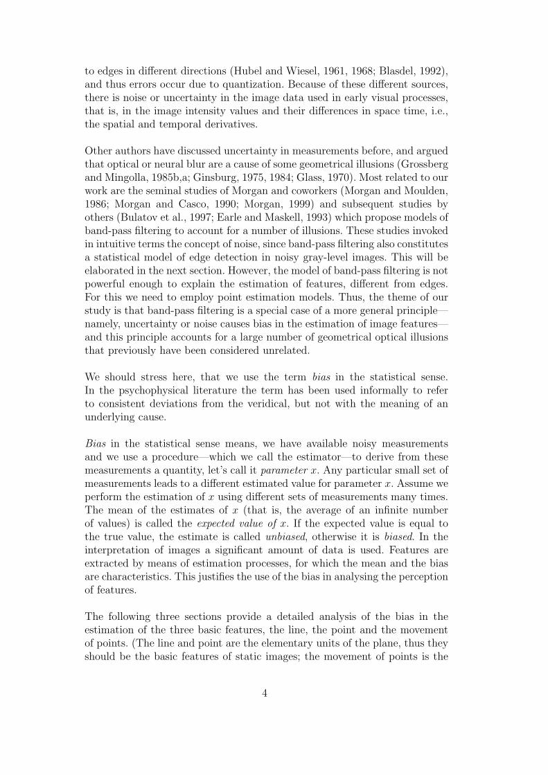
Expressed in our formalism of equation (6), this takes the following form. Theeffect of the gradient distribution on the bias is strongest in the direction of theeigenvector corresponding to the smaller eigenvalue of M ′ and weakest in theorthogonal direction. Changing the ratio of measurements (edgels) along thedifferent lines changes the bias. Figure 13 illustrates, for the case of a verticalline intersecting an oblique line at an angle of 30 degrees, the bias in the x- andy-directions as a function of the ratio of edge elements. It can be seen that asthe ratio of vertical to oblique elements increases, the bias in the x-directiondecreases and the bias in the y-direction increases. The Poggendorff illusion isstronger when the parallel lines are vertical or horizontal, because in this casethe bias parallel to the lines (along the y-axis in the plot) is larger, and theZollner illusion is stronger when the small lines are horizontal and vertical andthe main lines are tilted, as in this case the bias perpendicular to the mainlines (along the x-axis in the plot) is larger.

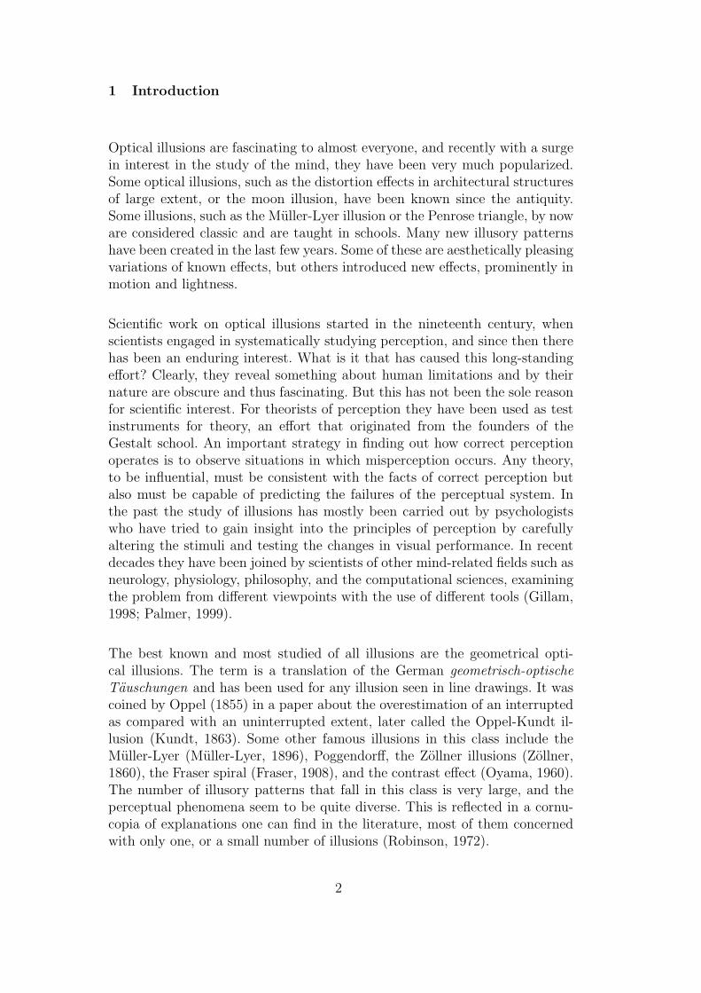
Many other well-known illusions can be explained on the basis of biased lineintersection. Examples are the Orbison figures (Orbison, 1939), Wundt’s figure(Wundt, 1898), and the patterns of Hering (1861) and Lukiesh (1922). In thesepatterns geometrical entities such as straight lines, circles, triangles or squaresare superimposed on differently tilted lines, and they appear to be distorted.This distortion can be accounted for by the erroneous estimation of the tiltin the line elements between intersection points and the subsequent fitting ofcurves to these line elements.

Figure 14 illustrates the estimation of the curve in the Luckiesh pattern. Eachline has two edges, and we computed the intersection between any backgroundedge and circle edge (using configurations such as those in Figure 13a). This

18

φ

ratio

x

654321

-0.05

-0.06

-0.07

-0.08

bias in x, φ = π/6

ratio

y

654321

0.6

0.55

0.5

0.45

0.4

0.35

0.3

bias in y, φ = π/6

(a) (b) (c)

Fig. 13. (a) A vertical line intersecting a tilted line at an angle φ = π/6 (the lengthof the vertical and the tilted line is one unit and σ = 0.06). (b) Bias perpendicularto the vertical as a function of the ratio of edge elements on the vertical and tiltedlines. (c) Bias parallel to the vertical.

provided for every intersection of the circle with a straight line four intersectionpoints, two corresponding to the inner edges of the circle and two to theouter ones. Arcs on the circle between two consecutive background lines wereapproximated by straight lines. (The ratio of elements between the circle andthe background edge was 2:1 (resulting in a configuration similar to that ofFigure 15 with the arc corresponding to the vertical.) – Note, other ratios givequalitatively similar results.) Consecutive intersection points—one originatingfrom an obtuse and one from an acute angle—were connected with straightline segments. Bezier splines were then fitted to the outer line segments. Thisresulted in a curve like the one we perceive, with the circle being bulbed outon the upper and lower left and bulbed in on the upper and lower right.

Next, let us look at the erroneous estimation of angles. Assuming that theerroneously estimated intersection point has a distorting effect on the arms(Wallace, 1969), the bias discussed for the above illusions will result in theoverestimation of acute angles. The underestimation of obtuse angles can beexplained if we assume an unequal amount of edgel data on the two arcs.Figure 15 illustrates the bias for acute and obtuse angles for the case of moreedge elements on the vertical than on the tilted line. The bias in the x-directionchanges sign and the bias in the y-direction increases (with increasing angle)for obtuse angles, and this results in a small underestimation of obtuse angles.

We used the intersection point as main criterion to explain the illusions dis-cussed in this section. But very likely many of these illusions are due to theestimation of multiple features. In particular, for illusions involving many smallline segments, such as the Zollner pattern, estimation of edges and estimationof intersection points would have very similar results.

Illusions of intersecting lines have been intensely studied, and there are alsomodels that employ in some form the concept of noise. Morgan and Casco(1990) propose as explanation of the Zollner and Judd illusion bandpass fil-

19

(a) (b)

(c) (d)

Fig. 14. Estimation of Luckiesh pattern: (a) the pattern: a circle superimposed on abackground of differently arranged parallel lines, (b) fitting of arcs to the circle, (c)magnified upper left part of pattern with fitted arcs superimposed, (d) intersectionpoints and fitting of segments to outer intersections.

φ2.521.510.5

0.02

0x

-0.02

-0.04

-0.06

bias in x, ratio = 3

φ

y

2.521.510.5

0.8

0.6

0.4

0.2

bias in y, ratio = 3

Fig. 15. A vertical line and a tilted line of length 1 intersecting at an angle φ; Theratio of vertical to tilted edge elements is 3 : 1; σ = 0.06 (a) Bias perpendicular tothe vertical. (b) Bias parallel to the vertical.

20

tering followed by feature extraction in second stage filters. The features arethe extrema in the band-pass filtered image, which correspond to the inter-section points. Morgan (1999) studied the Poggendorff illusion and suggestssmoothing in second stage filters as the main cause.

4 Bias in motion

When processing image sequences some representation of image motion mustbe derived as a first stage. It is believed that the human visual system com-putes two-dimensional image measurements which correspond to velocity mea-surements of image patterns, called optical flow. The resulting field of mea-surements, the optical flow field, represents an approximation to the projectionof the field of motion vectors of 3D scene points on the image.

Optical flow is derived in a two-stage process. In a first stage the velocitycomponents perpendicular to linear features are computed from local imagemeasurements. This one-dimensional velocity component is referred to as “nor-mal flow” and the ambiguity in the velocity component parallel to the edgeis referred to as the “aperture problem.” In a second stage the optical flow isestimated by combining, in a small region of the image, normal flow measure-ments from features in different directions, but this estimate is biased.

We consider a gradient-based approach to deriving the normal flow. The basicassumption is that image gray level does not change over a small time interval.Denoting the spatial derivatives of the image gray level I(x, y, t) by Ix, Iy, thetemporal derivative by It, and the velocity of an image point in the x- andy-directions by ~u = (u, v), the following constraint is obtained:

Ixu + Iyv + It = 0 (7)

This equation, called the optical flow constraint equation, defines the com-ponent of the flow in the direction of the gradient (Horn, 1986). We assumethe optical flow to be constant within a region. Each of the n measurementsin the region provides an equation of the form (7) and thus we obtain theover-determined system of equations

Is~u + ~It = 0, (8)

where Is denotes, as before, the matrix of spatial gradients (Ixi, Iyi

), ~It thevector of temporal derivatives, and ~u = (u, v) the optical flow. The least-squares solution to (8) is given by

~u = −(I tsIs)

−1ITs

~It. (9)

21

As a noise model we consider zero-mean i.i.d. noise in the spatial and temporalderivatives, and for simplicity, equal variance σ2

s for the noise in the spatialderivatives.

The statistics of (9) are well understood, as these are the classical linear equa-tions. The expected value of the flow, using a second-order Taylor expansion,is derived in appendix A; it converges to

limn→∞

E(~u) = ~u′ − σ2s( lim

n→∞(1

nM ′))−1~u′, (10)

where, as before, the actual values are denoted by primes.

Equation (10) is very similar to eq. (6) and the interpretation given thereapplies here as well. It shows that the bias depends on the gradient distribution(that is, the texture) in the region. Large biases are due to large variance,ill-conditioned M , or an ~u which is close to the eigenvector of the smallesteigenvalue of M . The estimated flow is always underestimated in length, andit is closer in direction to the direction of the majority of normal flow vectorsthan the veridical.

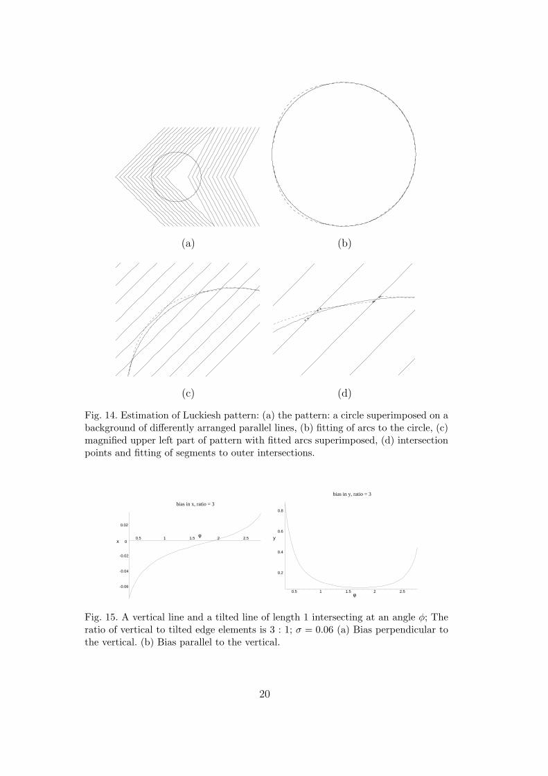
Figure 16 shows a variant of a pattern created by Ouchi (1977). The pat-tern consists of two rectangular checkerboard patterns oriented in orthogonaldirections—a background orientation surrounding an inner ring. Small retinalmotions, or slight movements of the paper, cause a segmentation of the insetpattern, and motion of the inset relative to the surround. This illusion hasbeen discussed in detail in (Fermuller et al., 2000). We will thus only give ashort description here.

The tiles used to make up the pattern are longer than they are wide leadingto a gradient distribution in a small region with many more normal flow mea-surements in one direction than the other. Since the tiles in the two regionsof the figure have different orientations, the estimated regional optical flowvectors are different. The difference between the bias in the inset and the biasin the surrounding region is interpreted as motion of the ring. An illustrationis given in Figure 17 for the case of motion along the first meridian (to theright and up). In addition to computing flow, the visual system also performssegmentation, which is why a clear relative motion of the inset is seen.

Another impressive illusory pattern from (Pinna and Brelstaff, 2000) is shownin Figure 18. If fixating on the center and moving the page (or the head ) alongthe optical axis back and forth the inner circle appears to rotate—clockwisewith a motion of the paper away from the eyes. For a backward motion ofthe paper the motion vectors are along lines through the image center, point-ing away from the center. The normal flow vectors are perpendicular to theedges of the parallelograms. Thus the estimated flow vectors are biased in the

22

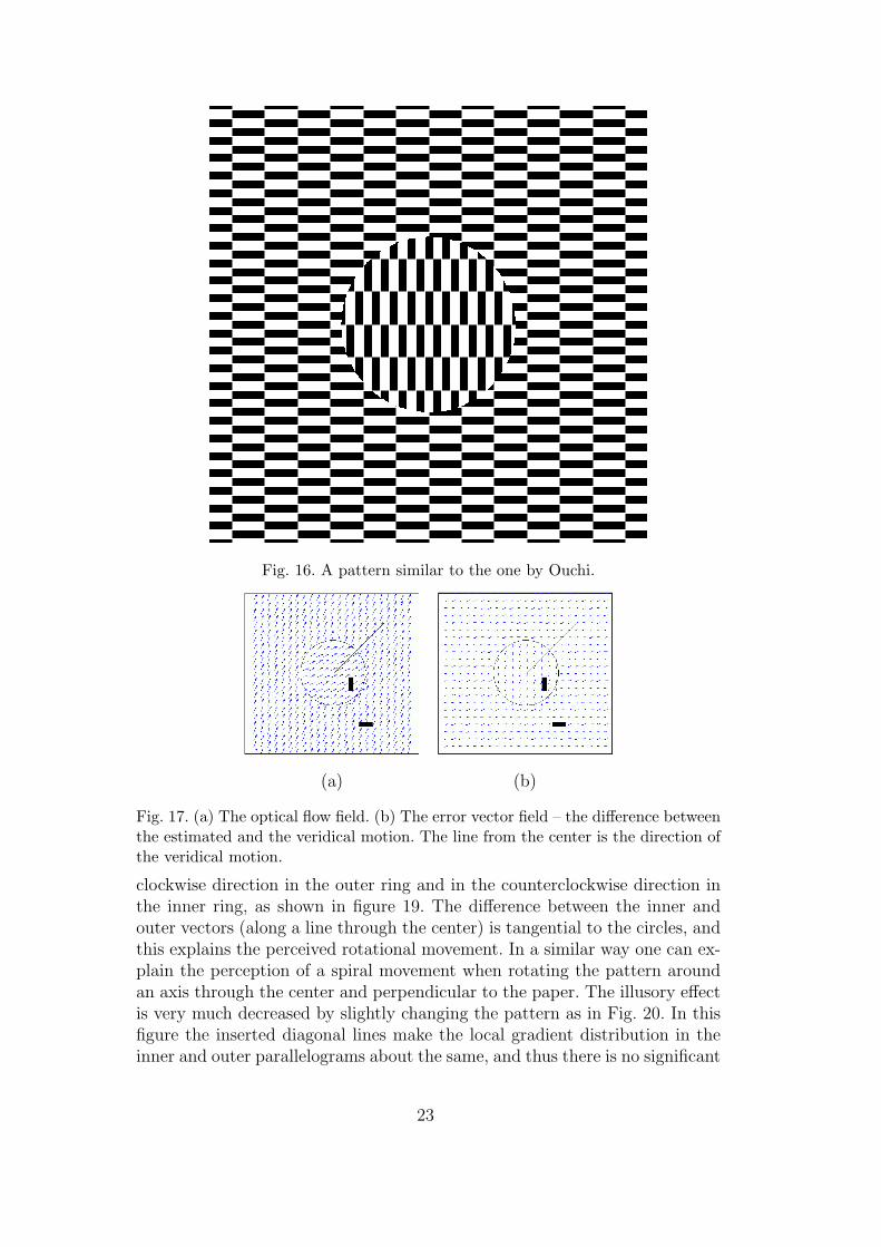
Fig. 16. A pattern similar to the one by Ouchi.

(a) (b)

Fig. 17. (a) The optical flow field. (b) The error vector field – the difference betweenthe estimated and the veridical motion. The line from the center is the direction ofthe veridical motion.

clockwise direction in the outer ring and in the counterclockwise direction inthe inner ring, as shown in figure 19. The difference between the inner andouter vectors (along a line through the center) is tangential to the circles, andthis explains the perceived rotational movement. In a similar way one can ex-plain the perception of a spiral movement when rotating the pattern aroundan axis through the center and perpendicular to the paper. The illusory effectis very much decreased by slightly changing the pattern as in Fig. 20. In thisfigure the inserted diagonal lines make the local gradient distribution in theinner and outer parallelograms about the same, and thus there is no significant

23

Fig. 18. If fixating on the center and moving the paper along the line of sight, theinner circle appears to rotate.

Fig. 19. Flow field computed from Figure 18.

difference in bias which could cause the perception of motion.

To be more rigorous, the estimation is somewhat more elaborate. The visionsystem not only computes normal flow and flow on the basis of the raw image.It also smoothes, or blurs, the image and computes normal flow and flow fromthe blurred image. That is, the vision system utilizes flow at different levelsof resolution. For the pattern here the flow vectors at different resolutions arein the same orientation, thus there will be no difference whether the systemused multiple resolutions or not. However, one may modify the pattern by

24

Fig. 20. Modification of Figure 18 reduces the illusory motion.

changing the black and white in the edges, thus creating bias in one directionat high resolution and bias in the other direction at low resolution, and thisway reduce the illusion (as in Figure 6 in (Pinna and Brelstaff, 2000)).

Helmholtz (1962) describes an experiment with the Zollner pattern whichcauses illusory motion. When the point of a needle is made to traverse Zollner’spattern (Figure 11a) horizontally from right to left, its motion being followedby the eye, a perception of motion in the bands occurs. The first, third, fifthand seventh black bands ascend, while the second, fourth, and sixth descend;it is just the opposite when the direction of the motion is reversed.

The bias predicts this effect as follows: A motion of the eyes from right to leftgives rise to optical flow from left to right. For each band there are two differ-ent gradient directions, i.e., there are two different normal flow componentsin each neighborhood. For the odd bands the two normal flow componentsare in the direction of the flow and diagonally to the right and up. Thus theestimated flow makes a positive angle with the actual flow (that is, it has apositive y-component), and this component along the y-axis is perceived asupward motion of the bands (see Figure 21). For even bands the estimatedflow is biased downward, causing the perception of descent of the bands. Sim-ilarly, if the motion of the eye is reversed the estimated flow has a negativey-component in the odd bands and a positive y-component in the even bands,leading to a reversal in the perceived motions of the bands.

We need to clarify here two issues. First, the simple model of constant flow in aneighborhood in general is not adequate to model image motion. We have used

25

u

n1n2

u′

Fig. 21. The eye motion gives rise to flow u′ and normal flow vectors n1 and n2.The estimated flow, u, has a positive y-component, which causes illusory motionupward in the band.

this model here for the purpose of a simple analysis. This model is sufficientonly for translational motions parallel to the image plane. In the general casewe have to segment the flow field at the discontinuities and within coherentregions allow for spatially smooth variation of the flow (Horn and Schunk,1981; Hildreth, 1983). Smoothness may be modeled by describing the flow asa smooth function of position, or by minimizing, in addition to the deviationfrom the flow constraint equation, a function of the spatial derivatives of theflow. But the principle of bias is still there (Fermuller et al., 2001).

Second, there are three models for computing optical flow in the literature.Besides gradient-based models there are frequency domain and correlationmodels, but computationally they are not very different. In all the modelsthere is a stage in which smoothness assumptions are made and measure-ments within a region are combined. At this stage noisy estimates lead tobias (Fermuller et al., 2001).

There is a large number of motion experiments that also can be explained byour model.

A significant body of work on the integration of local velocity signals hasbeen conducted in the context of moving plaids. Plaids are combinations oftwo wave gratings of different orientation, each moving with a constant speed.For any such “moving plaid” there is always some planar velocity the wholepattern can undergo which would produce exactly the same retinal stimulus.Depending on the parameters of the component gratings, the perception is ofone coherent motion of the plaid or of two different motions of the gratings.

The motion of a coherent pattern can be found theoretically with the inter-section of constraint model (IOC) – the vector component obtained from eachindividual grating constrains the local velocity vector to lie upon a line invelocity space, the intersection of the lines defines the motion of the plaid(Adelson and Movshon, 1982). However, often the perceived motion is differ-ent from the veridical. The error is influenced by factors including orientationof the gratings, frequency, and contrast.

26

Ferrera and Wilson (1987) made a distinction between two kinds of plaids; intype I plaids the common motion is between the components motions of thetwo gratings, and in type II plaids the common motion lies outside the compo-nent directions. In case of equal contrast and frequency, for type II plaids thevelocity is perceived towards the average of the component vectors (the VA)(Ferrera and Wilson, 1990, 1991; Burke and Wenderoth, 1993), whereas fortype I plaids the estimate is largely veridical. For type I plaids if the contrastof the gratings is different the perceived velocity is closer in direction to thecomponent of the grating of higher contrast (Stoner et al., 1990; Kooi et al.,1992). If the spatial frequency of the gratings differs (Smith and Edgar, 1991),the perceived motion is closer in direction to the gradients of higher spatialfrequency than the IOC velocity. In no case is there an overestimate of theplaid velocity when compared to the IOC prediction.

Recalling that the plaid velocity is biased in direction toward the eigenvectorof the larger eigenvalue of M

′, we can predict the expected bias from changes

in the plaid pattern. For components of equal contrast and frequency, themajor eigenvector is in the direction of the vector average of the componentmotion vectors. In type II plaids this results in an estimated flow towards theVA direction. If the contrast of one grating increases, the major eigenvectormoves towards the direction of motion of that grating explaining the findingsof (Stoner et al., 1990; Kooi et al., 1992). Higher frequencies in a directionamount to more measurements in that direction. In the case of orthogonalgratings, as in (Smith and Edgar, 1991) this results in an estimated flow closerin direction to the motion of the higher frequency.

Mingolla et al. (1992) studied stimuli consisting of lines moving behind aper-tures. The lines had one of two different orientations. For a motion to theright, and lines at orientation of 15◦ and 45◦ from the vertical, that is whenthe normal flow components were in the first quadrant (upwards and right)the motion appeared upward biased. With the normal flow components in thesecond quadrant (downwards and right – the lines at −15◦ and −45◦ from thevertical) the motion appeared downward biased and for symmetric lines (+15◦

and −15◦) the motion was perceived as horizontal. As in the case of type IIplaids, this can be predicted from the bias in flow estimation which changesthe direction of the estimated flow towards the vector average direction.

Circular figures rotating in the image plane may not give the perception of arigid rotation (Musatti, 1924; Wallach, 1935). The effect is well known for thespiral which appears to contract or expand depending whether the rotationis clockwise or counterclockwise. For a rotation around the spiral’s center themotion vectors are tangential to circles and the normal flow vectors are closeto the radial direction. This situation creates large bias in the regional estima-tion of flow and thus an additional motion component in the radial directionas illustrated in Fig.22. This illusion, among many others, has been explained

27

by Hildreth (1983) by means of a model of smooth flow. The smoothness con-straint also contributes to radial motion as it penalizes positional change inflow. As discussed above, a complete flow model also needs to consider varia-tion in the flow. However, even with small amounts of noise, the contributionof the bias to the radial motion component will be larger than the contributionfrom smoothness.

Fig. 22. A spiral rotating in the clockwise direction gives rise to a flow field withradially inward pointing vectors. The flow was derived using LS estimation withinsmall circular regions. (No smoothness constraints were enforced.)

Noise in the normal flow measurements has been discussed before as a pos-sible cause for misperceived motion. In (Nakayama and Silverman, 1988a,b)and (Ferrera and Wilson, 1991) Monte Carlo experiments were performed todetermine the expected value and variance of velocity calculated with the IOCmethod. The experiments proceeded by creating one-dimensional motion com-ponents which were corrupted with error of Gaussian distribution, and thencomputing for pairs of local velocity measurements the motion vector with theIOC model. The distribution of estimates created with this method was notfound to be significantly biased away from the IOC prediction (Ferrera andWilson, 1991) for the case of plaids, but the variance of these estimates wasfound to be correlated with the accuracy of directional perception (Nakayamaand Silverman, 1988a).

Nakayama and Silverman (Nakayama and Silverman, 1988a,b) found thatsmooth curves, including sinusoids, Gaussians and sigmoids may be perceivedto deform non-rigidly when translated in the image plane. For example, a si-nusoid with low curvature (due to low amplitude or low frequency) movingwith horizontal translation appears to deform non-rigidly, while the same mo-tion for a sinusoid of high curvature appears veridical. In this case the maindifference between the two curves lies in the amount of biased regional flowestimates as illustrated in Figure 23. The flow field in Figures 23a and b were

28

(a) (b)

(c) (d)

Fig. 23. (a) and (b) Regional LS estimation of flow. (c) and (d) Flow estimationusing smoothness constraints.

estimated using LS estimation within small regions. As can be seen, in regionsnext to the inflexion point the flow vectors are biased upward on one sideand downward on the other, and these regions are much smaller in the curvewith larger curvature. The flow fields in Figures 23c and d were estimated byenforcing in addition smoothness constraints. The smoothness propagates thebias, resulting in vertical flow components which are upward in half of the lowcurvature sinusoid and downward in the other half. In comparison the bias ismuch less in the high curvature sinusoid, effecting only the areas at the centerof the curve.

Nakayama and Silverman (1988a) attributed the phenomenon to the largevariance in the distribution of flow estimates. Clearly, the bias in regionalflow estimates and the variance of the distribution of all the estimates arecorrelated; the larger the bias, the larger the variance. As Nakayama andSilverman (1988a) point out, the variance should be a good measure for theprocess of segmentation, that is to decide on coherence or non-coherence.

29

Simoncelli et al. (1991) and Weiss and Adelson (1998) also discuss noise in thenormal flow estimates, but they only consider noise in the temporal derivatives.These noise terms do not cause bias; it is the noise in the spatial derivatives(i.e. the orientation of the local image velocity components) which causes bias.Weiss and Adelson, however, conclude bias in flow estimation using Bayesianmodeling. Their explanation is based on the assumption that there is an a pri-ori preference for small flow values. It is easily understood that this preferenceresults in an increase in the a posteriori probabilty of small flow values andthus a bias towards underestimation of the flow, and thus a flow estimationsimilar to ours. Note, thus, in the Bayesian model the bias is in effect assumed,whereas in our model it is not. 1

5 The theoretical question

The natural question to ask is whether the bias is due to the particular com-putations we described, or whether it is an inherent problem. In other words,is the estimation of features biased in whatever way it is conducted, or is biasa feature only of linear estimation? Are there other methods which don’t suf-fer from bias to begin with, or is it maybe possible to estimate the bias andthen correct for it? Our answer is, in general it is not. This section is a briefstatistical discussion explaining what could be done, why it is very hard tocorrect for the bias and that the theoretically best thing to do is to partiallycorrect for it.

The mathematical problem at hand (for edge intersection and flow estimation)is to find a solution to an over-determined system of equation of the formA~x = ~b. The observations A and ~b are corrupted by noise, i.e. A = A′ + δAand ~b = ~b′ + δ~b. In addition there is system error, ~ε (because the equations

are only approximations), and thus A′~x = ~b′ +~ε. We are dealing with, what iscalled in statistical regression the errors in variable (EIV) model.

It is well know, that the least squares (LS) estimator is biased (Fuller, 1987).

The LS solution, which is linear in ~b, is an asymptotically unbiased estimatoronly, when the errors δA are zero and the errors δ~b are independent.

The classical way to address the problem is by means of the corrected leastsquares (CLS) estimator. If the statistics of the noise, that is the covariancematrix of δA, were known, an asymptotically unbiased linear estimation couldbe obtained. The problem is that for small amounts of data, accurate estima-tion of the variance of the noise is a very difficult problem. In this case, the

1 The Non-Bayesian method of LS estimation implicitly also assumes priors; itassumes that all solutions have equal probability.

30

estimation of the variance is not accurate, leading to large variance for CLS.

In recent years the technique of total least squares (TLS) has received a lotof attention. The basic idea underlying this nonlinear technique is to dealwith the errors in A and ~b symmetrically. If all the errors in δA and δ~b areidentical and independent, TLS is asymptotically unbiased. In the case theyare not, one would need to whiten the data. But this requires the estimationof the ratio of the error variances δA and δ~b, which is at least as hard asobtaining the variance of δA. An incorrect value of the ratio often results inan unacceptably large over correction for the bias. However, the main problemfor TLS is system error. Theoretically one can use multiple tests to obtain themeasurement errors, like re-measuring or re-sampling; but unless the exactparameters of the model are known, one cannot test for system error.

Resampling techniques, such as bootstrap and Jacknife have been discussedfor bias correction. These techniques can correct for the error term which isinverse proportional to the number of data points (i.e. O( 1

n)), and thus they

can improve the estimate of the mean for unbiased estimators. However, thesetechniques cannot correct for the bias (Efron and Tibshirani, 1993). They areuseful for estimating the variance in order to provide confidence intervals.

Why is it so difficult to obtain accurate estimates of the noise parameters?To acquire a good noise statistic a lot of data is required, so data needs to betaken from large spatial areas acquired over a period of time, but the modelsused for the estimation can only be assumed to hold locally. Thus to integratemore data, models of the scene need to be acquired. Specifically, in the caseof intersecting lines, first long edges and bars need to be detected, and in thecase of motion, first discontinuities due to changes in depth and differentlymoving entities need to be detected and the scene segmented. If the noiseparameters stayed fixed for extended periods of time it would be possible toacquire enough data to closely approximate these parameters, but usually thenoise parameters do not stay fixed long enough. Sensor characteristics maystay fixed, but there are many other sources of noise besides sensor noise. Thelighting conditions, the physical properties of the objects being viewed, theorientation of the viewer in 3D space, and the sequence of eye movements allhave influences on the noise.

Clearly, bias is not the only thing that matters. There is a trade-off betweenbias and variance. Generally, an estimator correcting for bias increases thevariance while decreasing the bias. Very often, the mean squared error (MSE)is used as a criterion for the performance of an estimator. It is the expectedvalue of the square of the difference between the estimated and the true value.If x′ is used to denote the actual value, x to denote the estimate, and E(.) todenote the expected values, the MSE is defined as

31

MSE(x) = E((x− x′)2) = (E(x)− x′)2 + E(x′ − E(x))2

= bias2(x) + cov(x), (11)

that is, as the sum of the square of the bias (denoted as bias(x)) and thevariance (denoted as cov(x)). Based on the criterion of minimizing the MSE,there are compromised estimators which outperform both uncorrected biasedestimators and corrected unbiased estimators. The ideal linear estimator wouldperform a partial bias correction using CLS. In appendix B we derive howmuch this correction (theoretically) should be. It depends on the covarianceof the LS estimates. The larger the covariance, the less correction.

This brings us to the point of a psychometric function describing quantitativelythe effects of noise on the perception. We should assume that our vision systemis doing its best and thus has learned to correct whenever it has data availableto obtain estimates of the noise. Since the correction should depend on thevariance, a measure of misestimation should involve both the bias and thevariance of the LS estimator; we suggest to investigate a weighted sum of thesetwo components. Such a measure may explain why the illusory perceptionin some of the patterns weakens after extended viewing, in particular whensubjects are asked to fixate ((Helmholtz, 1962; Yo and Wilson, 1992). In thiscase, we can assume the noise parameters stay fixed, and the visual systemcan reasonably well estimate them. Furthermore, such a measure would predictthat the density of a pattern should have an influence on the perception, withslightly more accurate estimates for denser patterns.

Finally, one may think there are ways to correct the bias without using statis-tics. The bias depends on the gradient distribution, that is the directions ofedgels or motion measurements. Since an uneven distribution (correspondingto an ill-conditioned matrix M) leads to a large bias, one may want to nor-malize for direction. We could do so, if we had very large amounts of data.However, with few measurements we cannot. Consider that there are only twodirections. It would mean that we give more weight to the direction with fewmeasurements, which has large variance, and lesser weight to the other direc-tion which has smaller variance. With few measurements only, this could leadto large over-correction.

Also, it should be clear that in our models of feature estimation, we cannotemploy higher level knowledge about the structure of the scene. For example,computing the intersection of lines by first estimating the average directionof each individual line and then intersecting the lines, would not give bias.But, this would require that the noisy elements are classified first into twocategories. The same applies for the flow in plaids. If we wanted to estimate themotion of the individual gratings, we would first need to understand that thereare exactly two different directions and classify the motion components. If, as

32

in (Ferrera and Wilson, 1991) pairs of noisy measurements are intersected,and the elements are randomly sampled (without classifying them first) therewill be a bias in the direction of the flow component with more measurements.If the elements are segmented and each pair has an element of either grating,there should be a slight overestimation in magnitude. This is, because theunderestimation in LS results from the asymptotic behavior; terms linear in1n

or higher do not effect the bias, but these terms for very few measurements,i.e two in this case, cause a bias in the opposite direction.

6 Discussion

6.1 Theories of Illusions

Theories about illusions have been formulated ever since their discovery. Manyof the theories are aimed only at one specific illusion and most of the earlytheories would be seen nowadays as adding little to a mere description ofthe illusion. Most theories which attempt to explain a broad spectrum ofillusions are based on a specific sort of mechanism which has been suggested toexplain the workings of human visual perception. These mechanisms are eitherhypothetical, based on physical analogies, or general observations about thephysiology and architecture of the brain (for example, lateral inhibition). Thetheory proposed here is of a mathematical nature based on the geometry andstatistics of capturing light rays and computing their properties (gray valuesand spatio-temporal derivatives), and thus it applies to any vision system,artificial or biological. However, one might find that our theory resemblessome existing theories if they are put in a statistical framework.

Chiang (1968) proposed a retinal theory that applies to patterns in which linesrunning close together affect one another. He likened the light coming into theeye from two lines to the light falling onto a screen from two slit sources inthe study of diffraction patterns. This is because of the blurring and diffusingeffect of the medium and the construction of the eye. The perceived loca-tions of the lines are at the peaks of their distributions; thus two close linesinfluence each other’s locations and become one when the sum of their distri-butions forms a single peak. This leads to an overestimation of acute angles,and provides an explanation of the Zollner, Poggendorff, and related illusionsas well as the Muller-Lyer effect. Glass (1970) discussed optical blurring asa cause for the perceptual enlargement of acute angles as it fills in the angleat line intersections and he proposed this as an explanation of the Zollnerand Poggendorff effect. Ginsburg argued that neural blurring occurs becauseof lateral inhibition and this has the effect of spatial frequency filtering. In(Ginsburg, 1975) he suggested that low frequency attenuation contributes to

33

the formation of the illusory Kanizsa triangle and in (Ginsburg, 1984) he dis-cussed filtering processes as a cause for the Muller-Lyer illusion. In a number ofrecent studies band-pass filtering has been proposed as a cause of geometricaloptical illusions; Morgan and Moulden (1986), and Earle and Maskell (1993)discuss linear band-pass filters as a cause of the cafe wall illusion. Morganand Casco (1990) discuss band-pass filtering in conjunction with second-orderstage filters that extract features in the Zollner and Judd illusion. Bulatovet al. (1997) propose an elaborate neurophysiological model and they discussthe Muller-Lyer and Oppel-Kundt illusion. (Morgan, 1999) suggests blurringin second stage filters as the main cause of the Poggendorff illusion and (Mor-gan and Glennerster, 1991; Morgan et al., 1990) discuss large receptive secondstage eclectic units, which obtain as input heterogeneous features from smallersubfields, as cause for the Muller-Lyer illusion.

The diffraction in Chiang’s model, the optical and neural blurring in latermodels, amounts to uncertainty in the location of the perceived gray levelvalues, or they can be interpreted as noise occurring somewhere in the imageformation or the image processing. Thus the concept of uncertainty is invokedin vague ways in these studies. The models that have been discussed are,however, very restricted. They apply to particular processes, either on theretina or the neural hardware.

There are a number of theories in which eye movements are advanced asan important causative factor in illusions. Our theory also proposes that eyemovements play a role because they are a relevant source of noise. The partic-ular eye movements made in looking at a pattern influence the noise distribu-tion and thus the bias perceived, but there are other noise sources besides eyemovements, and this predicts the existence of illusory effects for some patternseven under fixation or tachistoscopic viewing.

Helmholtz (1962) suggested that ocular movements are of importance in someillusions, but he also expressed doubt that they could be the main source, asother illusions are not influenced by them. Carr (1935) proposed that the eyesreact to accessory lines and as a result pass more easily over unfilled than filledelements. In the Muller-Lyer figures the eyes move more freely over the figurewith outgoing fins than over the one with ingoing fins, and in the Poggendorffand Zollner figures deflections and hesitations in the eye movements are asso-ciated with the intersections of the long lines with the obliques. Piaget (1961)proposed a “law of relative centrations.” By “centration” he refers to a kindof centering of attention which is very much related to fixation. Centrationon part of the field causes an overestimation of that part relative to the restof the field. Virsu (1971) suggested that a tendency to eye movements, thatis, instructions for eye movements, has a perceptual effect. He suggests thatthe eye movements most readily made are linear and rectilinear, horizontalor vertical. When viewing lines which lie off the vertical or horizontal, an

34

eye movement correction must take place and this can give rise to perceptualdistortion.

Other theories include those whose main objective was the explanation offigural aftereffects applied to illusions (Ganz, 1966; Kohler and Wallach, 1944).In these theories interference between nearby lines occurs because of satiationin the cortex or lateral inhibition processes. There are also theories based onthe assumption that the perceptual system interprets illusory patterns as flatprojections of three-dimensional displays (Tausch, 1954; Thiery, 1896). Themost detailed and most popular such theory is due to Gregory (1963), whoinvokes “size constancy scaling,” which can be triggered in two different ways,either unconsciously or by higher-level awareness.

6.2 Illusions of size

Following Boring (Boring, 1942), patterns which are called geometrical op-tical illusions may be classified roughly into two categories: illusions of di-rection (where orientation of a line or figure is misjudged) and illusions ofextent (where size or length is misjudged). The patterns discussed so far arein the first class. They have been explained on the basis of noise in the localmeasurements. Most illusions in the second class could be explained if noisewere present in the representations of quantities which cover larger regions.Such noise may be attributed to the processing in the visual system. Fromevidence we have about the varying size of receptive fields, it is understoodthat images are processed at multiple levels of resolution (Zeki, 1993). Sincethe higher-level processes of segmentation and recognition need informationfrom large parts of the image, there must be processes that combine informa-tion from local neighborhoods into representations of global information, andthese processes may carry uncertainty.

Intuitively, noise effecting regions of larger spatial extent, causes blurring overthese regions. Thus, neighboring parts in a figure influence each other and as aresult they are perceived closer in distance. This observation can explain mostof the significant illusions in the second class which are: the contrast effect;the illusion of filled and unfilled extent, that is, the effect that a filled extentis overestimated when compared with an unfilled extent (an example is theOppel-Kundt illusion (Kundt, 1863)); the framing effect, that is, the overes-timation of framed objects; and the flattening of arcs, that is, the effect thatshort arcs are perceptually flattened. Take as an example the Delboeuf illu-sion (Delboeuf, 1892)—two concentric circles with the outer one perceptuallydecreased and the inner one increased. Blurring which effects both circles willcause the inner one to expand and the outer one to contract. Another exampleis the famous Muller-Lyer illusion. Bias in the intersection points due to noise

35

in local measurements can account for a small size change in the vertical lines,but it requires noise in larger regions to account for significant size changes asexperienced with this pattern. Similarly, such noise will increase the effect inthe Poggendorff illusion, and it may account for the perception in variationsof this pattern.

6.3 Bias in 3D

Many other computations in the visual system, besides feature extraction, areestimation processes. Clearly, the visual recovery processes are estimations –that is, the computations which extract physical and geometrical propertiesof the scene by inverting the (optical and geometrical) image formation. Ex-amples are the estimations of the light source, the motion, the structure andshape of the scene and the material properties of surfaces.

We recently started investigating these computations. Results are availablefor shape from motion, stereo and texture from all three known cues, that isforeshortening, scaling and position (Hui and Fermuller, 2003). We analyzedthe bias and found that it is consistent with what is empirically known aboutthe estimation of shape. It has been observed from computational as well aspsychophysical experiments, that for many configurations there is a tendencyto underestimate the slant. (The slant refers to the angle between the surfacenormal and the optical axis.) In other words, the scene appears compressed inthe depth dimension. The bias predicts this underestimation of slant.

We created an illusory display demonstrating the effect for 3D motion whichcan be viewed at (Fermuller, 2003). It shows a plane with two textures, one inthe upper half, one in the lower half. The camera moves around the plane whilefixating on its center. Because the bias in the upper texture is much largerthan in the lower one, the plane appears to be segmented into two parts, withthe upper part of much smaller slant. This should demonstrate our point. Thebias not only is a problem of 2D vision, but of 3D vision as well.

A Expected Value of the Least Squares Solution

In this section a second-order Taylor expansion of the expected values of theleast squares solution for both the intersection point (Section 3) and the flow(Section 4) is given.

Let ~y be the vector to be estimated, that is, either the intersection point ~xor the flow ~u. Is is the matrix consisting of the spatial derivatives Ixi

, Iyi. ~c

36

in Section 3 is the vector of temporal derivatives Iti and ~c in Section 4 is thevector whose elements are Ixi

x0i+ Iyi

y0i.

The expected value E(~y) of the least squares solution is given by

E(~y) = E((IT

s Is)−1(IT

s ~c))

As the noise is assumed to be independent and zero-mean, the first-order termsas well as the second-order terms in the noise of the temporal derivatives (orthe positional parameters) vanish. This means that it is only the noise in thespatial derivatives which causes bias in the mean. The expansion at pointsN = 0 (i.e., δIxi

= δIyi= δIti = 0 or δIxi

= δIyi= δx0i

= δy0i= 0) can be

written as

E(~y) = ~y′ +∑

i

(∂2~y

∂δI2xi

⌋N=0

E(δI2xi

)

2+

∂2~y

∂δI2yi

cN=0

E(δI2yi

)

2

)

For notational simplicity, we define

M = ITs Is and ~b = IT

s ~c

M ′ = I ′sT I ′s

~b′ = I ′sT ~c′

To compute the partial derivatives, the explicit terms of the matrix M are

M =

∑i

(I ′xi

+ δIxi

)2 ∑i

(I ′xi

+ δIxi

) (I ′yi

+ δIyi

)∑

i

(I ′xi

+ δIxi

) (I ′yi

+ δIyi

) ∑i

(I ′yi

+ δIyi

)2

and the terms of ~b are

~b =

∑i

(I ′xi

+ δIxi

) (I ′ti + δIti

)∑

i

(I ′yi

+ δIyi

) (I ′ti + δIti

)

and

~b =

∑i

(I ′xi

+ δIxi

)2 (x′0i

+ δx0i

)+(I ′xi

+ δIxi

) (I ′yi

+ δIyi

) (y′0i

+ δy0i

)∑

i

(I ′xi

+ δIxi

) (I ′yi

+ δIyi

) (x′0i

+ δx0i

)+(I ′yi

+ δIyi

)2 (y′0i

+ δy0i

)

Using the fact that for an arbitrary matrix Q

−∂Q−1

∂x= Q−1∂Q

∂xQ−1

37

we find the first-order and second-order derivatives to be

∂~y∂δIxi

= −M−1

[2Ixi

Iyi

Iyi0

]M−1~b + M−1 ∂~b

∂δIxi

∂2~y∂δI2

xi

= 2M−1

[2Ixi

Iyi

Iyi0

]M−1

[2Ixi

Iyi

Iyi0

]M−1~b

−M−1

[2 0

0 0

]M−1~b

−2M−1

[2Ixi

Iyi

Iyi0

]M−1 ∂~b

∂δIxi+ M−1 ∂2~b

∂δI2xi

and similarly we have symmetric expressions for

∂~y

∂δIyi

and∂2~y

∂δI2yi

Since we assume E(δI2xi

) = E(δI2yi

) = σ2s , the expansion can thus be simpli-

fied to

E(~y) = ~y′ − nM ′−1~y′σ2s +

∑ni=1 M ′−1

(∂2~b

∂δI2xi

+ ∂2~b∂δI2

yi

)⌋N=0

σ2s

2

+∑

i

{M ′−1

([2I ′xi

I ′yi

I ′yi0

]M ′−1

[2I ′xi

I ′yi

I ′yi0

]

+

[0 I ′xi

I ′xi2I ′yi

]M ′−1

[0 I ′xi

Ixi2I ′yi

])~y′

−M ′−1

([2I ′xi

I ′yi

I ′yi0

]M ′−1 ∂~b

∂δIxi

⌋N=0

+

[0 I ′xi

I ′xi2I ′yi

]M ′−1 ∂~b

∂δIyi

⌋N=0

)}σ2

s

where we have underlined the terms that do not depend on n (where n is thenumber of measurements being combined in a region). These terms will givea consistent, statistically constant response. The rest of the terms diminishproportionally to 1

n. Informal experiments show that these terms become neg-

ligible for n > 5, a number clearly smaller than the number of terms likely tobe combined in any real system.

38

In the analysis of Section 3, the elements of ~c are Ixix0i

+ Iyiy0i

; thus

∂~b∂δIxi

⌋N=0

=

2I ′xix′0i

+ I ′yiy′0i

I ′yix′0i

∂2~b∂δI2

xi

⌋N=0

=

2x′0i

0

∂~b

∂δIyi

⌋N=0

=

I ′xiy′0i

I ′xix′0i

+ 2I ′yiy′0i

∂2~b∂δI2

yi

⌋N=0

=

0

2y′0i

and the main terms in the expected value of the intersection point E(~x) are

E(~x) = ~x′ − nM ′−1~x′σ2s + M ′−1

[Σx′0i

Σy′0i

]σ2

s

or

E(~x) = ~x′ + nM ′−1(~x′0 − ~x′)σ2s ,

where ~x′0 denotes the mean of the values ~x′0i.

In the analysis in Section 4 the elements of ~c are Iti . Thus the first-orderderivatives are

∂~b

∂δIxi

⌋N=0

=

[I ′ti

0

]and

∂~b

∂δIyi

⌋N=0

=

[0

I ′ti

],

and the second-order derivatives vanish. The expected value of the flow E(~u)simplifies to

E(~u) = ~u′ − nM ′−1~u′σ2s .

B Bias Correction

Let us write the equation system as A~x = ~b. Let ~xLS denote the LS estimatorfor the errors in variable model. It’s expected bias amounts to

bias(~xLS) = limn→∞

E(~xLS − ~x′) = −σ2( limn→∞

(1

nA′T A′))−1~x′.

39

Assuming the variance of the error δA is known, the bias can be removed withthe CLS estimator, which amounts to

~xCLS = (AT A− nσ2I)−1(AT~b),

and can be rewritten as

~xCLS = (I − nσ2(AT A)−1)−1~xLS.

Denoting the variance as cov(.), the variance of ~xCLS amounts to

cov(~xCLS) = (I − nσ2(AT A)−1)−2cov(~xLS).

Let us now investigate what the theoretically best linear estimator should be.We have to adjust the corrected least squares estimator, such that we achievesmaller MSE (as defined in equation (11)). Let xα = α~xCLS + (1 − α)~xLS

denote the adjusted CLS estimator.

Then we have that

MSE(xα) = α2cov(~xCLS) + (1− α)2bias2(~xLS)

= α2(I − nσ2(AT A)−1)−2cov(~xLS) + (1− α)2bias2(~xLS).

which is a quadratic expression. Thus, the MSE minimum is achieved for

α =bias2(~xLS)

bias2(~xLS) + cov(~xLS)(I − nσ2(AT A)−1)−2.

This shows that according to the MSE criterion a less bias corrected xα isbetter than a bias corrected ~xCLS. The larger the variance of the LS estimates,the less the correction should be.

References

Adelson, E. H., Movshon, J. A., December 1982. Phenomenal coherence ofmoving visual patterns. Nature 300, 523–525.

Blasdel, G. G., 1992. Differential imaging of ocular dominance and orientationselectivity in monkey striate cortex. Journal of Neuroscience 12, 3115–3138.

Boring, E. G., 1942. Sensation and perception in the history of experimentalpsychology. Appleton-Century-Crofts, New York.

Bulatov, A., Bertulis, A., Mickiene, L., 1997. Geometrical illusions: Study andmodelling. Biological Cybernetics 77, 395–406.

40

Burke, D., Wenderoth, P., 1993. The effect of interactions betwen one-dimensional component gratings on two-dimensional motion perception. Vi-sion Research 33, 343–350.

Cameron, E., Steele, W., 1905. The Poggendorff illusion. Psychol. Monogr. 7,83–107.

Canny, J., 1986. A computational approach to edge detection. IEEE Transac-tions on Pattern Analysis and Machine Intelligence 8, 679–698.

Carpenter, R. H. S., 1988. Movements of the Eye. Pion, London.Carr, H. A., 1935. An Introduction to Space Perception. Longmans, Green,

New York.Chiang, C., 1968. A new theory to explain geometrical illusions produced by

crossing lines. Percept. Psychophys. 3, 174–176.Delboeuf, J. L. R., 1892. Sur une nouvelle illusion d’optique. Bull. de l’Acad.

roy. de Belg. 24, 545–58.Earle, D. C., Maskell, S., 1993. Fraser cords and reversal of the cafe wall

illusion. Perception 22, 383–390.Efron, B., Tibshirani, R., 1993. An introduction to the boostrap. Chapman &

Hall.Fermuller, C., 2003. http://www.optical-illusions.org.Fermuller, C., Pless, R., Aloimonos, Y., 2000. The Ouchi illusion as an artifact

of biased flow estimation. Vision Research 40, 77–96.Fermuller, C., Shulman, D., Aloimonos, Y., 2001. The statistics of optical flow.

Computer Vision and Image Understanding 82, 1–32.Ferrera, V. P., Wilson, H. R., 1987. Direction specific masking and the analysis

of motion in two dimenions. Vision Research 27, 1783–1796.Ferrera, V. P., Wilson, H. R., 1990. Perceived direction of two-dimensional

moving patterns. Vision Research 30, 273–287.Ferrera, V. P., Wilson, H. R., 1991. Perceived speed of moving two-dimensional

patterns. Vision Research 31, 877–893.Fraser, J., 1908. A new visual illusion of direction. Brit. J. Psychol. 2, 307–320.Fuller, W., 1987. Measurement Error Models. Wiley, New York.Furmanski, C., Engel, S., 2000. An oblique effect in human primary visual

cortex. Nature Neuroscience 3, 535–536.Ganz, L., 1966. Mechanism of the F.A.E.’s. Psychol. Rev. 73, 128–150.Gillam, B., 1998. Perception and Cognition at Century’s End. Academic Press,

Ch. Illusions at Century’s End, pp. 95–136.Ginsburg, A. P., 1975. Is the illusory triangle physical or imaginary? Nature

257, 219–220.Ginsburg, A. P., 1984. Visual form perception based on biological filtering. In:

Spillman, L., Wooton, B. R. (Eds.), Sensory Experience, Adaptation andPerception. L. Erlbaum, New Jersey, pp. 53–72.

Glass, L., 1970. Effect of blurring on perception of a simple geometric pattern.Nature 228, 1341–1342.

Green, R., Hoyle, G., 1964. Adaptation level and the optic-geometric illusions.Nature 201, 1200–1201.

41

Gregory, R. L., 1963. Distortion of visual space as inappropriate constancyscaling. Nature 119, 678.

Grossberg, S., Mingolla, E., 1985a. Neural dynamics of form perception:Boundary completion, illusory figures, and neon color spreading. Psycho-logical Review 92 (2), 173–211.

Grossberg, S., Mingolla, E., 1985b. Neural dynamics of perceptual grouping:Textures, boundaries and emergent segmentations. Perception and Psy-chophysics 38 (2), 141–171.

Helmholtz, H. L. F. V., 1962. Treatise on Physiological Optics. Vol. III. Dover,New York, translated from the Third German Edition by J. P. C. Southall.

Hering, E., 1861. Beitrage zur Psychologie. Vol. 1. Engelman, Leipzig.Hildreth, E., 1983. The Measurement of Visual Motion. MIT Press, Cam-

bridge, Massachusets.Horn, B. K. P., 1986. Robot Vision. McGraw Hill, New York.Horn, B. K. P., Schunk, B. G., 1981. Determining optical flow. Artificial In-

telligence 17, 185–203.Howard, I., Templeton, W., 1966. Human Spatial Orientation. Wiley, New

York.Hubel, D., Wiesel, T., 1968. Receptive fields and functional architecture of the

monkey striate cortex. J. Physiol. (Lond.) 195, 215–243.Hubel, D. H., Wiesel, T. N., 1961. Integrative action in the cat’s lateral genic-

ulate body. J. Physiol. (Lond.) 155, 385–398.Hui, J., Fermuller, C., 2003. Uncertainty in 3d shape estimation. In: Proc.

3rd International Workshop on Statistical and Computational Theories ofVision. p. to appear.

Judd, C., Courten, H., 1905. The Zollner illusion. Psychol. Monogr. 7, 112–139.Kitaoka, A., 2003. http://www.ritsumei.ac.jp/~akitaoka/index-e.html.Koenderink, J. J., 1984. The structure of images. Biological Cybernetics 50,

363–370.Kohler, W., Wallach, H., 1944. Figural after-effects: An investigation of visual

processes. Proc. Amer. Philos. Soc. 88, 269–357.Kooi, F. L., Valois, K. K. D., Grosof, D. H., Valois, R. L. D., 1992. Properties of

the recombination of one-dimensional motion signals into a pattern motionsignal. Perception and Psychophysics 52, 415–424.

Kundt, A., 1863. Untersuchungen uber Augenmaß und optische Tauschungen.Pogg. Ann. 120, 118–158.

Leibowitz, H., Toffey, S., 1966. The effects of rotation and tilt on the magni-tude of the Poggendorf illusion. Vision Research 6, 101–103.

Lindeberg, T., 1994. Scale-Space Theory in Computer Vision. Kluwer, Boston.Lukiesh, M., 1922. Visual illusions. Dover, New York.Marr, D., Hildreth, E. C., 1980. A theory of edge detection. Proc. Royal So-

ciety, London B 207, 187–217.Mingolla, J., Todd, J., Norman, J., 1992. The perception of globally coherent

motion. Vision Research 32, 1015–1031.Morgan, M. J., 1999. The Poggendorff illusion: a bias in the estimation of

42

the orientation of virtual lines by second-stage filters. Vision Research 39,2361–2380.

Morgan, M. J., Casco, C., 1990. Spatial filtering and spatial primitives in earlyvision: An explanation of the Zollner-Judd class of geometrical illusions.Proc. Royal Society, London B 242, 1–10.

Morgan, M. J., Glennerster, A., 1991. Efficiency of locating centres of dotclusters by human observers. Vision Research 31, 2075–2083.

Morgan, M. J., Hole, G., Glennerster, A., 1990. Biases and sensitivities in thegeometrical illusions. Vision Research 30, 1793–1810.

Morgan, M. J., Hoptopf, N., 1989. Perceived diagonals in grids and lattices.Vision Research 29, 1005–1015.

Morgan, M. J., Moulden, B., 1986. The Munsterberg figure and twisted cords.Vision Research 26 (11), 1793–1800.

Morinaga, S., 1933. Untersuchungen uber die Zollnersche Tauschung. Jap. J.Psychol. 8, 195–242.

Muller-Lyer, F. C., 1896. Zur Lehre von den optischen Tauschungen: UberKontrast und Konfluxion. Z. Psychologie 9, 1–16.

Musatti, C., 1924. Sui fenomeni stereocinetici. Archivio Italiano di Psicologia3.

Nakayama, K., Silverman, G. H., 1988a. The aperture problem - I. Perceptionof nonrigidity and motion direction in translating sinusoidal lines. VisionResearch 28, 739–746.

Nakayama, K., Silverman, G. H., 1988b. The aperture problem - II: Spatialintegration of velocity information along contours. Vision Research 28.

Oppel, J. J., 1855. Uber geometrisch-optische Tauschungen. JahresberichtPhys. Ver. Frankfurt , 37–47.

Orbison, W., 1939. Shape as a function of the vector field. Amer. J. Psychol.52.

Ouchi, H., 1977. Japanese and Geometrical Art. Dover, New York.Oyama, T., 1960. Japanese studies on the so-called geometrical-optical illu-

sions. Psychologia 3, 7–20.Palmer, S. E., 1999. Vision Science: Photons to Phenomenology. MIT Press,

Cambridge, MA.Piaget, J., 1961. Les Mechanismes Perceptifs. Presses Universitaires de Gravee,

translated by G. N. Seagrim as The Mechanisms of Perception, Routledge& Kegan Paul, London, 1969.

Pinna, B., Brelstaff, G. J., 2000. A new visual illusion of relative motion.Vision Research 40 (16), 2091–2096.

Robinson, J. O., 1972. The Psychology of Visual Illusion. Hutchinson, London.Simoncelli, E. P., Adelson, E. H., Heeger, D. J., 1991. Probability distributions

of optical flow. In: Proc. IEEE Conference on Computer Vision and PatternRecognition. Maui, Hawaii, pp. 310–315.

Smith, A. T., Edgar, G. K., 1991. Perceived speed and direction of complexgratings and plaids. Journal of the Optical Society of America 8, 1161–1171.

Stoner, G. R., Albright, T. D., Ramachandran, V. S., 1990. Transparency and

43

coherence in human motion perception. Nature 344, 153–155.Tausch, R., 1954. Optische Tauschungen als artifizielle Effekte der

Gestaltungsprozesse von Großen und Formkonstanz in der naturlichenRaumwahrnehmung. Psychol. Forsch. 24, 299–348.

Thiery, A., 1896. Uber geometrisch optische Tauschungen. Phil. Stud. 12, 67–126.

Virsu, V., 1971. Tendencies to eye movement, and misperception of curvature,direction and length. Percept. Psychophys. 9, 65–72.

Wagner, H., 1969. Simultaneous and successive contour displacements. Ph.D.thesis, University of Wales.

Wallace, G., 1969. The critical distance of interaction in the Zollner illusion.Percept. Psychophys. 5, 261–264.

Wallace, G., Crampin, D., 1969. The effects of background density on theZollner illusion. Vision Research 9, 167–177.

Wallach, H., 1935. Uber visuell wahrgenommene Bewegungsrichtung. Psychol-ogische Forschung 20, 325–380.

Weiss, Y., Adelson, E. H., 1998. Slow and smooth, a Bayesian theory for thecombination of local motion signals in human vision. AI Memo 1616, MIT.

Witkin, A. P., 1983. Scale-space filtering. In: Proc. International Joint Con-ference on Artificial Intelligence. pp. 1019–1022.

Wundt, W., 1898. Die geometrisch-optischen Tauschungen. Abhandl. math-phys. der sachs. Ges. Wiss. 24, 53–178.

Yo, C., Wilson, H. R., 1992. Moving 2D patterns capture the perceived di-rection of both lower and higher spatial frequencies. Vision Research 32,1263–1270.

Yuille, A., Poggio, T., 1986. Scaling theorems for zero-crossings. IEEE Trans-actions on Pattern Analysis and Machine Intelligence 8, 15–25.

Zeki, S. M., 1993. A Vision of the Brain. Blackwell, London.Zollner, F., 1860. Uber eine neue Art von Pseudokopie und ihre Beziehungen

zu den von Plateau and Oppel beschriebenen Bewegungsphanomenen. Ann.Phys. Chem. 186, 500–523.

44