Unemployment Insurance asan Economic Stabilizer:Evidence of Effectiveness Over Three Decades Unemployment InsuranceOccasional Paper 99-8

U.S. Department of LaborAlexis M. Herman, Secretary

Employment and Training AdministrationRaymond L. Bramucci, Assistant Secretary

Unemployment Insurance ServiceGrace A. Kilbane, Director

Division of Research and PolicyEsther R. Johnson, Chief

1999

This report was prepared for the U.S. Department of Labor, Employment and Training Administration, Unemployment Insurance Service by Coffey Communications, LLC under contract number G-5914-6-00-87-30 (5). Its authors are Lawrence Chimerine, Theodore S. Black, and Lester Coffey. Since contractors conducting research and evaluation projects under government sponsorship are encouraged to express their own judgement freely, this report does not necessarily represent the official opinion or policy of the 4U.S. Department of Labor. The UIOP Series presents research findings and analyses dealing with unemployment insurance issues. Papers are prepared by research contractors,staff members of the unemployment insurancesystem, or individual researchers. Manuscripts and comments from interested individuals are welcome. All correspondence should be sent to:

UI Occasional PapersUnemployment Insurance ServiceFrances Perkins Building, Room S-4231200 Constitution Avenue, N.W.Washington, DC 20210email: UIOPapers@doleta.gov

Unemployment Insurance as an Automatic Stabilizer:Evidence of Effectiveness Over Three Decades

Lawrence Chimerine, Theodore S. Black, and Lester CoffeyCoffey Communications, LLC

Martha K. Matzke, Editor

July 1999

TABLE OF CONTENTS

Chapter Page

EXECUTIVE SUMMARY 4

INTRODUCTION 10

I THE UI PROGRAM AND ECONOMIC STABILIZATION 11

II UI AS AN AUTOMATIC STABILIZER: DESCRIPTIVE ANALYSIS 16

III REVIEW OF RECENT LITERATURE 27

IV IS THE BUSINESS CYCLE OBSOLETE? 37

V EVIDENCE OF THE ABSOLUTE EFFECTIVENESS OF UI

AS AN AUTOMATIC STABILIZER: A SIMULATION ANALYSIS 60

VI EVIDENCE OF THE RELATIVE EFFECTIVENESS OF UI

AS AN AUTOMATIC STABILIZER FOR THE U.S. ECONOMY 79

VII CONCLUSIONS AND RECOMMENDATIONS 84

APPENDICES

A The Unemployment Insurance Equation 87

B The WEFA Model 88

C Simulation Results 91

D Estimates of Relation Between UI and the Economy 96

E Interpolation of Federal Supplemental Benefits (FSB) by Quarter 100

F Estimates of Relation Between Net UI Financial Flows and the Changes in Federal Tax Receipts 102

G Bibliography 106

H Glossary of Terms 119

LIST OF FIGURES AND TABLES

Chapter Page

II UI AS AN AUTOMATIC STABILIZER: DESCRIPTIVE ANALYSIS 16 Table 1 Regular Unemployment Taxes and Benefits 17Figure 1 UI Benefit Expenditures 19Figure 2 Percentage of Workers Covered vs. Percentage

of Wages Subject to UI Tax 22Figure 3 Unemployment Insurance Claimants 24Figure 4 Total Recipiency: Regular, Extended,

Supplemental 25

IV IS THE BUSINESS CYCLE OBSOLETE? 37Figure 1 Average Length of Business Cycle Expansion 48Figure 2 Inventory/Sales Ratio 49Table 1 Postwar Recessions 50Figure 3 Service Industry Employment as a Percentage

of Total Jobs 51Figure 4 Distribution of Wealth, 1983-95 52Table 2 Percent of Total Assets by Wealth Class, 1995 53Figure 5 Share of Total Stock Market Gains, 1989-97,

by Wealth Class 54Table 3 Selected Measures of Household Income

Dispersion 55Figure 6 Share of Aggregate Household Income

by Quintile 56Figure 7 Percent Change in Household Gini Coefficients 57Table 4 After Tax Distribution of Income 58Figure 8 Family Income Average Annual Change 59

V EVIDENCE OF THE ABSOLUTE EFFECTIVENESS OF UI AS AN AUTOMATIC STABILIZER 60Table 1 Recession Dates 62Table 2 Ratio of Lost UI Benefits to Lost GDP

by Recession 63

Figure 1 GDP Loss Prevented by UI Program 64Figure 2 UI Impacts on Real GDP Due to Monetary

Shocks 65Figure 3 Average Difference in Real GDP From Baseline 66

Figure 4 Percent of Simulated GDP Recession Loss Offsetby UI: Average of All Monetary Shock ScenarioReplicates 67

Table 3 Income Expansion Multipliers and Job Impacts 68Table 4 GDP and Real UI Benefit Impact 69Figure 5 Net UI vs. Delta GDP 70Table 5 Ratio of Change in Net UI to Change in GDP 71Table 6 UI Equation Results 76Table 7 Coefficient Equivalence Tests 77

VI EVIDENCE OF THE RELATIVE EFFECTIVENESS OF UI

AS AN AUTOMATIC STABILIZER FOR THE U.S. ECONOMY 79

Table 1 Peak-to-Trough Changes 80Figure 1 Net UI vs. Delta Fed Tax 82

APPENDIX ATable A-1 The WEFA Unemployment Insurance Equation 87

APPENDIX CTable C-1 Impact of Monetary Policy Experiments 91Table C-2 Recession Without Unemployment Insurance

Actual vs. Simulation 94APPENDIX D

Table D-1 UI Equation Results 97Table D-2 Chapter V Model Equation Results 98Table D-3 Coefficient Equivalence Tests 98

APPENDIX ETable E-1 Estimates of FSB Participants 101

APPENDIX FFigure F-1 Net UI vs. Delta Fed Tax [Lagged 3 Quarters] 103

ACKNOWLEDGMENTS

Several individuals made significant contributions to this project. Dr. Esther Johnson of the

U.S. Department of Labor, Employment and Training Administration, Unemployment Insurance

Service (UIS) was extraordinarily insightful in providing guidance on appropriate ways to address

policy considerations. In addition, she gave the authors the latitude to experiment with innovative

approaches and offered prompt and careful feedback on several alternatives considered, as well as on

preliminary drafts of the report. Tom Stengle of UIS did a superb job in supplying necessary

Unemployment Insurance data and information and in explaining some of the subtleties in the UI data.

John Heinberg, also of UIS, offered many useful suggestions for maintaining an audience-friendly focus

in the crafting of the report.

Daniel Bachman of WEFA, Inc., ran the macro-economic simulations for this study and

supplied much helpful analytical and technical background information.

At Coffey Communications, LLC, Amy Coffey assisted with proofreading and providing a

reality check for non-economists. Nick Liu provided vital data and graphics support. Randall T.

Ferrell contributed computer and research skills that helped immensely.

EXECUTIVE SUMMARY

In recent years, some economists and policymakers have come to believe that the federal-state

unemployment insurance (UI) system plays an ever-diminishing role as a stabilizing force in the U.S.

economy. This report takes a fresh look at UI’s effectiveness and relative importance as an automatic

economic stabilizer. The report reviews the arguments made by critics of the program, updates previous

quantitative studies of UI’s economic stabilization effect, and introduces a new, expanded model to test

the program’s effectiveness over the last 25 years. The report concludes there is no evidence to support

the view that the structure of the economy has changed in any way that diminishes the effectiveness of the

UI program. This conclusion is demonstrated by the econometric analyses, simulations, and other statistical

measurements undertaken in this study.

Most analysts who argue that UI holds declining importance as a countercyclical economic

stabilizer base their conclusions on qualitative indicators that they perceive to reflect fundamental changes

in the U.S. economy. They point to the dampening of business cycles since World War II and the huge

increase in household wealth, for example, as evidence of diminishing need for UI’s countercyclical role.

This study argues that such an interpretation ignores key evidence of widening inequality in income

distribution, rising consumer debt, continuing downsizing and layoffs, and growing needs for worker

retraining, to name only some of the factors that make the need for UI as a countercyclical safety net as

great today as it has ever been.

To demonstrate UI’s effectiveness, the study undertakes a major quantitative analysis of the

program’s countercyclical cushioning impact. It examines this effect on an absolute basis using the

historical data, and on a relative basis, compared against federal tax receipts. This analysis goes beyond

previous work on this subject in several regards: It includes data from the 1990-91 recession; it includes

both absolute and relative measurements of UI’s effectiveness; and it offers both aggregate findings on the

overall UI program and findings on the effectiveness of UI’s individual component programs (regular,

extended, and supplemental).

Specifically, this study shows that:

1) The argument that structural changes, including a dampening of the business cycle,

have reduced the need for the countercyclical unemployment insurance program is not supported

by the evidence.

a) Some analysts cite the rapid rise in household wealth as a sign of the declining usefulness of

unemployment insurance. They argue that family savings now act as a powerful economic

cushion during lean times. This study contends that the rise in wealth is, itself, cyclical to some

extent, reflecting the rise in stock prices of recent years. This paper wealth can be reduced

suddenly, as it was during the market correction of mid-1998. More important, the rise in

wealth has been lopsidedly in the top tier of household income (Federal Reserve data show

that the share of household wealth declined between 1983 and 1995 for all but the wealthiest

1 percent of the population). Growing consumer debt levels across the income spectrum also

suggest that the family wealth hypothesis for weathering recessions is exaggerated. Moreover,

those who lose, or cannot get, jobs tend disproportionately to be those with little or no savings

or wealth in the first place.

b) Some analysts argue that the rise of the service sector over manufacturing is contributing to the

virtual elimination of business cycles. But the evidence shows that the emergence of the service

sector began long before the current era and has not prevented recessionary cycles.

Moreover, during the post-World War II period, a period often cited as one of milder

recessions than those of pre-World War II, there have been several very steep economic

declines accompanied by high unemployment. In virtually all of these recessions, the

unemployment rate rose even after the trough in GDP. Further, many jobs in the manufacturing

sector have migrated into manufacturing services as a result of outsourcing. These jobs, not

counted in manufacturing employment statistics, are nonetheless heavily impacted by any

weakness in manufacturing.

c) Another contention is that the less-severe post-World War II recessions are themselves

evidence that underlying structural changes are dampening business cycles. This study argues,

as have most students of business cycles, that government safety-net programs -- including the

countercyclical UI program -- are one major reason for the dampening phenomenon, not

fundamental changes in the structure of the U.S. economy. Moreover, increased economic

globalization is likely to give policymakers less control over the economy in the future than has

been the case in the past; in particular, such factors as recessions in other countries, sharp

changes in exchange rates that affect trade flows, sudden shifts in capital flows, oil shocks, and

other global supply shocks increase the potential for recessions caused by events external to

the U.S. economy. Steep oil-price increases largely caused the economic downturns in 1973

and 1980, but some downplay the importance of these events by noting that the oil-related

recession of 1990-91 was milder. That recession, however, was part of a prolonged period

of near-stagnant growth that was among the lowest-growth periods since World War II. There

is no real evidence on the record that recessions would be milder in the absence of the array

of federal programs providing stabilization.

2) UI continues to be an effective automatic stabilizer in the U.S. economy.

Like the last major study of UI as an economic stabilizer (Dunson, et al, 1990, known as the Metrica

study), this study employs econometric models of the economy to examine changes in the countercyclical

effectiveness of UI and to determine the magnitude of those changes. Wharton Econometric Forecasting’s

Quarterly Model (the WEFA Model) was adopted because of its capabilities in modeling complex macro-

economic relationships involving multiple variables, and because the WEFA Model has established a

remarkable track record in the accuracy of its predictions.

Two types of analysis were performed to measure UIs effectiveness over time, with the

following findings:

a) Five historical recessions beginning in 1969 were examined using counter-factual simulations.

These recession scenarios were studied with and without the effects of UI. The simulations

showed that the UI program mitigated the loss in real GDP by about 15 percent over all the

quarters in each recession. When multipliers were calculated (the expansionary effect of each

UI dollar added to the economy) for each recession, the impact of UI in the 1990=s recession

was found to be more robust than in the 1980's recession, although less so than in the 1970's

recession. The WEFA model showed that over the five recessionary periods, the average

peak annual number of jobs saved was 131,000. While the simulations showed a decline in

annual jobs saved during the 1980s as compared with the prior decade, the number rose

slightly in the 1990s.

b) A single descriptive equation was also estimated to measure the effectiveness of UI and the

supplemental programs in the recessions of the 1970s, 1980s (this period includes the short

recession of 1980 and the deeper one of 1981-82), and early 1990s. The results indicate that

the UI program exhibits a substantial and statistically significant countercyclical effect on

changes in real GDP throughout these decades. The equation showed that the recessions over

the three decades, as measured by the decline in real GDP, would have been an average of

17 percent deeper if the UI program did not exist. This result is comparable to the 15 percent

produced by the WEFA analysis. Likewise, the evidence for the supplemental programs of UI

suggests that, while they were most effective in the 1970s and their effectiveness declined in

the 1980s, during the 1990s their effectiveness rebounded.

c) A current what if simulation of a recession beginning in November 1998 showed that by the

middle of the year 2000, UI would be pumping $10 billion to $15 billion a year (in 1992

dollars, the baseline currently used by WEFA) into the macro-economy, moderating the

recession and speeding up the recovery. This simulation corroborated the historical evidence

that UI’s impact as an automatic stabilizer has not decreased significantly over time and that

it would remain important in a future recession.

These findings counter the conclusion of the 1990 Metrica study B on the basis of evidence from

the recessions of the 1970s and 1980s that UI probably was becoming significantly less effective as an

automatic stabilizer over time. The two wholly separate analytical techniques (simulations and descriptive

equation) applied in the current study produced closely aligned results showing continuity in UI effectiveness

over three decades.

The current study’s finding of a greater cushioning effect by UI, as compared with the Metrica

study, reflects a variety of differences in the approaches of the two studies. A key distinction is that the

current study focuses on the total macro-economic stimulus represented by all UI expenditures during

recessions (including UI’s extended and supplemental benefits programs as well as its regular benefits

program). Although the extended and supplemental benefits admittedly are not wholly automatic, the

perspective of this study is that the UI program’s effectiveness as an economic stabilizer is a function of

the totality of the economic stimulus it provides to shore up the economy during economic downturns. To

assess that overall stimulus, the current study analyzes for the first time the aggregate economic impact of

all three tiers of UI benefits (regular, extended, and supplemental), as well as the individual economic stimuli

provided by the supplemental benefits programs enacted during the last three recessions. There were major

discontinuities in the historical data on extended benefits in the Metrica data sets, and the study did not

include data on the supplemental UI programs.

In addition, the two studies used different econometric models, with different structures and inherent

multipliers, although it is difficult to quantify the precise effects of these factors. Part of the difference also

may be explained by the fact that Metrica measured UI’s cushioning effect based on one data point during

each recession. The current study uses an average of data points over time, considering that a more

effective approach. The findings of this study are in fact more consistent with the findings of prior analyses

-- for example, those of von Furstenburg (1976), de Leeuw, et al (1980), and McGibany (1983).

Other differences between the two studies include the economic specification for the benefit

equation used in the simulations, the use of GNP in Metrica and GDP in the current study, and the fact that

more timely and complete data sets were available for the current study.

Despite these differences, however, both the Metrica study and this study found evidence of

decreased UI effectiveness in the 1980s. But up to now, discussion of the effectiveness of UI as an

automatic stabilizer has been based primarily on work completed prior to the 1990-91 recession. This

study includes an examination of that recession, which provides significant new evidence that the program’s

countercyclical impact remains robust. This appears to reflect a slowing in the decline of the recipiency rate

for UI benefits.

3) The argument that UI has become less effective because other economic stabilizers

have become more effective or more important, is not supported by this study. UI may become

the primary automatic stabilizer in the years ahead.

One analytical test performed in this study produced suggestive evidence that the importance of

the UI program has increased relative to one of the primary fiscal-policy instruments for automatic

stabilization, changes in federal tax receipts. The analysis found that fluctuations in levels of federal tax

receipts have measurably diminished during recent recessionary episodes (most markedly in the 1990s),

when declines in real GDP would be expected to engender substantial reductions in automatic (progressive)

income tax receipts.

Holding discretionary monetary policy constant, such changes may mean that this historically

important countercyclical instrument is becoming less effective in its automatic stabilization role. The reasons

probably include the increasing importance of Social Security taxation, the tax treatment of capital gains,

and the declining progressivity of the income tax (realized compared to statutory) at the top end of the

income distribution, although research on this question is beyond the scope of this study.

It is not clear to what degree this finding, produced in the course of the analyses of the UI program’s

functioning in the macro-economy, predicts the pattern of future fluctuations in federal tax receipts. But the

finding represents at least preliminary evidence that the relative importance of the UI program as an

automatic stabilizer is increasing.

4) It may be possible to make the UI program even more effective as an automatic stabilizer by

refining its triggering and funding mechanisms.

Because the burden of automatic stabilization appears to be shifting to the UI program, this study

concludes it is imperative to examine ways to modify the aspects of the UI program that could make it more

effective as a stabilizer during economic downturns. In particular, such considerations would include finding

ways to: (1) Expand the basis of UI recipiency; (2) Make the UI extended and supplemental programs

(extension of benefits) more automatic and less subject to the political process, to ensure that they are not

only available, but available more quickly in the recessionary cycle, and (3) Strengthen the adequacy of the

programs financing mechanisms.

10

INTRODUCTION

The countercyclical effectiveness of the UI program reflects the capability to dampen fluctuations

in GDP during recessions and booms. In recent years, increasing attention has been directed towards the

UI program, questioning its relevance for current federal policy and the need for UI in today’s modern

global economy, and disputing the effectiveness of the program.

This study examines conceptual and empirical evidence regarding the countercyclical effectiveness

of the UI program. A set of absolute measures of effectiveness is developed and presented to show how

the UI program has functioned historically and to examine its current posture. In addition, the role UI plays

as an economic stabilizer is evaluated relative to federal tax receipts -- perhaps the major automatic

stabilizer in the economy.

An econometric analysis of the UI program is presented to assess the two permanent (regular and

extended) programs and the temporary supplemental programs enacted during recent recessions. The

WEFA macro-econometric model of the economy is used to obtain a set of simulations of the UI

program’s effectiveness. (In econometric methodology, simulations are said to be “counter-factual” in

nature. That is, they are hypothetical scenarios set up to depict structural characteristics of the economy

and the impacts of fiscal policy.) Other econometric results are presented to show aspects of both absolute

effectiveness and relative importance.

The study begins, in Chapter I, with a discussion of the theory of automatic economic stabilizers,

a description of UI as an economic stabilizer, and a brief history of the program. Chapter II examines the

historical evidence of UI’s countercyclical effectiveness over three decades and discusses key attributes

of the program. Chapter III reviews recent literature on UI as an economic stabilizer.

Chapter IV presents the main arguments by critics of the program and refutes them on the basis

of a variety of current economic events. It argues that the same structural shifts in the economy cited as

indicating the diminishing need for UI as a countercyclical stabilizer actually represent dangers to stability

that UI is uniquely positioned to counter. It concludes that the UI program not only is still necessary as a

component of U.S. economic policy, but also is more necessary than ever.

In Chapter V, findings are presented on absolute measures of UI’s effectiveness. Chapter VI

presents the evidence on relative measures of UI effectiveness. Chapter VII summarizes the study’s

conclusions and recommendations.

11

I. THE UI PROGRAM AND STABILIZATION

What Is an Automatic Stabilizer?

In principle, an automatic stabilizer acts to dampen fluctuations in the level of economic activity.

Automatic countercyclical programs are designed to ensure that fiscal injections or withdrawals occur in

a timely fashion, without design or implementation delays that accompany discretionary policy.

As an automatic stabilizer, a fiscal instrument works with no discretionary policy decisions required.

Recessionary declines in economic activity are met with expansionary levels of fiscal expenditure and

reduced taxes. Potential inflationary expansions are slowed by the increased levels of taxes and reduced

expenditure.

On balance, the tax and expenditure impacts work simultaneously. Although the momentum of each

instrument is in an opposite direction (one increases while the other declines), the effect on GDP is in the

same direction.

Taxes as Automatic Stabilizers

The effect of a tax in the economy may be described in macro-economic theory as a leakage of

expenditure. Taxes reduce the level of expenditure that may be sustained with a given level of income.

Changing the level of taxes levied on the economy will have an effect on the level of income in the opposite

direction.

Reducing taxation leads to increased aggregate expenditure for any level of pretax income. This

increased level of expenditure will have multiplier effects on the equilibrium level of pretax income. Thus

lowering taxation is expansionary.

Increases in the level of taxation have the opposite effect. Higher taxes reduce the level of

expenditure that may be attained for any level of income. The reduced level of expenditure has a multiplier

effect and consequently tax increases are likely to slow down the level of economic activity.

Fiscal Expenditures as Automatic Stabilizers

Public expenditures act as fiscal injections in the macro-economy. Fiscal injections also act on the

economy with a multiplier effect. Changes in government expenditures lead to changes in the level of

economic activity in the same direction.

Increasing public expenditure adds to the level of aggregate demand for a given level of

income. Macro-economic multiplier effects of the increased government expenditures work through the

economy and lead to increases in the level of income.

12

Decreased public expenditure slows the economy. Reducing government spending for a given level

of income reduces aggregate demand and aggregate expenditure. Multiplier effects amplify the initial

reduction and the level of equilibrium income will fall by more than the reduction in the level of public

expenditure.

Objectives of the Automatic Stabilizer

The application of an automatic stabilizer results in dampened fluctuations in the level of economic

activity. The swings of the business cycles are lessened. The severity of recessions is reduced and the

inflationary risks are reduced for an economy overheating during booms.

Why UI Works as an Automatic Stabilizer

The expenditures and taxes of the UI program act in tandem as an automatic stabilizer.

In the core UI program (regular and extended benefits), expenditures and taxes operate without external

intervention. That is, during periods of expansion and rising employment, taxes are collected automatically

according to pre-established guidelines. During economic contractions, employment levels fall, tax

collections slow, and benefit payouts rise to UI claimants under pre-established terms and conditions.

Consistent with the theory and empirical evidence of automatic economic stabilizers, these attributes

serve as counterbalances to the direction of the economy: During an expansion, UI taxation rises and UI

benefits fall, dampening inflationary pressures of economic growth. During a contraction, injections of UI

benefits flow into the economy and UI taxation decreases, moderating the contraction’s severity.

In addition, this countercyclical UI framework provides a positive psychological and stabilizing

benefit to the macro-economy. Because that impact is not quantifiable, however, the cushioning effect of

UI measured by this study probably underStates the overall stabilization impact of the program. The

ongoing payments of benefits and taxes through the UI system give all of its stakeholders--potential

recipients, employers, consumers, investors, and policymakers--the confidence to maintain their

consumption and investment patterns, knowing that the UI safety net is in place. The safety net thus relieves

stress, mitigates against overcautiousness in spending, and prevents large increases in the savings rate in

periods of economic volatility. Particularly during an economic downturn, sustaining confidence and

expectations prevents the recession from feeding on itself.

Moreover, even in a moderate recession, UI benefits relieve hardship for individuals. And the

evidence of this study confirms previous findings suggesting that the injection of UI benefits into the

economy during a recession helps turn the cycle upward again.

The UI program is not completely automatic in its economic stabilization role. There are currently

1 U.S. Department of Labor, Bureau of Employment Security 1950b, p.1

13

three tiers of UI benefits, each with a different level of automaticity. The regular benefits program is the

most fully automatic: regular UI benefits flow to qualified unemployed workers immediately, without any

external policy intervention required. Extended benefits, which flow to qualified claimants who have

exhausted their regular benefits, are less automatic: they become available when unemployment reaches a

specified “trigger” level. Supplemental UI benefit programs are the least automatic tier of UI benefits: they

become available only by an act of the U.S. Congress.

But all three tiers produce economic stabilization once they are in play. This study examines the

impact of benefit dollars from all three tiers of the UI program on the macro-economy.

History of the Federal-State UI Partnership

Since the depths of the Great Depression, the nation’s unemployment insurance program has

provided American workers with temporary income support during periods of involuntary unemployment.

Established under the Social Security Act of 1935 and subsequent state actions, the program finances

payments to unemployed individuals primarily through taxes on employers.

Though the Social Security Act contained no formal statement of the purposes for unemployment

insurance, early commentaries stressed protection against the hazard of unemployment, “regularization of

employment” (by having employers foot the costs through taxation), facilitating return to employment, and

maintenance of purchasing power -- and thus economic stability -- during contractions in the economy.

The Bureau of Employment Security described this latter purpose in a 1950 document as follows: “By

maintaining essential consumer purchasing power, on which production plans are based, the program

provides a brake on downturns in business activity, helps to stabilize employment, and lessens the

momentum of deflation during periods of recession.”1

The general framework of the Federal-State partnership undergirding the unemployment insurance

system has remained standing for nearly 65 years, although the details of the federal and state roles -- and

the balance between them -- have been constantly in evolution. Under the program, employers pay state

and federal employment taxes on employee wages. Within broad federal guidelines, States basically shape

and administer their programs individually, setting state taxation rules, eligibility criteria, and benefit levels.

State and federal UI tax receipts are held in a federal unemployment trust fund until they are needed.

Major milestones in the development of the UI program include federal actions from the 1950s to

the 1980s to extend coverage to most civilian workers and provide additional and emergency temporary

14

benefits for severe recessionary conditions. The first federal action to provide so-called “extended benefits”

came during the recession of 1958, when the Congress enacted a temporary extended benefits program

for workers who had exhausted their regular benefits. States could participate on a voluntary basis,

borrowing federal funds to make payments and returning the sums interest-free to the federal trust fund.

Proposals to make extended benefits a permanent part of the UI program were debated in the

1960s, but the concept did not become law until 1970. The Extended Benefits program allowed claimants

to receive additional benefits for up to 13 more weeks, or 50 percent of the duration of their original

coverage period. The cost was shared 50-50 by States and the federal government, and the federal

unemployment tax was raised by 0.1 percent to fund the federal government’s share. Under the law,

extended benefits were to be triggered when the unemployment level in a state reached a specified point;

the program could be triggered nationwide if the national insured unemployed rate reached a specified level.

Despite the addition of the Extended Benefits program to UI, the recessions of the 1970s, 1980s

(includes two recessions), and 1990s left severe long-term unemployment in their wake, with hundreds of

thousands of individuals having exhausted both regular and extended benefits. In each of these economic

contractions, federal lawmakers enacted temporary supplemental benefit programs financed solely by the

federal government. These emergency benefits programs, which provided payments beyond the 39th week

of unemployment, were tied to state unemployment rates as triggers. (Amendments to federal legislation

in the 1990s, however, made it possible for States to move more quickly to federal supplemental funds.)

The Federal Supplemental Benefits (FSB) program, enacted in late 1974, ran through March 1977. In the

next decade, the Federal Supplemental Compensation (FSC) program was enacted in September 1982

and was maintained until March of 1985. During the last recession examined in this study, that of 1990-91,

the Emergency Unemployment Compensation (EUC) program went into effect in November of 1991 and

ended in April of 1994.

Conclusions

Previous studies, as noted in this study’s literature review, have shown that the relative health of

the U.S. economy in recent decades may, at least in part, be attributed to the effectiveness of federal

economic policies designed to sustain the economy’s performance over time. The automatic stabilizers,

including the UI program, that dampen cyclical changes in the level of economic activity are among the

array of policy instruments contributing to this prosperity.

In their 1990 study of the federal unemployment insurance system, Dunson, et al, (Metrica study)

offered a variety of descriptive indicators of UI’s effectiveness as an automatic stabilizer over time. The

15

study concluded, however, that the evidence was at best ambiguous and seemed to point to a decrease in

UI’s effectiveness in the 1980s. But Metrica’s work did not cover the recession of the 1990s, and the

study’s analyses did not include either the Extended Benefits program or the temporary supplemental

programs.

This study presents historical and analytical evidence demonstrating that, during the last three

recessionary periods (1973-75, 1980-82 and 1990-91), the UI program performed as expected, with

evidence of some weakening of effectiveness in the 1980s but with a rebound of effectiveness in the 1990s.

The findings confirm the theory and prior empirical evidence of the impact of automatic stabilizers on the

economy, and show the continued effectiveness of UI in this regard.

16

II. UI AS AN AUTOMATIC STABILIZER: DESCRIPTIVE ANALYSIS

For the UI program to serve as an automatic stabilizer, without any intervention of government, it

should increase benefit expenditures during recessions and collect more UI taxes during recoveries.

Because the program is not 100 percent automatic, however, empirical evidence must be gathered and

analyzed to monitor the degree to which it helps smooth the fluctuations in business cycles over time. UI

is not completely automatic because its temporary components are activated only by Congressional action,

and because some of the governing regulations of its permanent components are determined by state

lawmaking.

In this review of the historical evidence of how the UI program functions in the macro-economy,

the focus is on whether the program exhibits the countercyclical responses that characterize an automatic

stabilizer. The review also examines related labor force trends and discusses possible implications of these

data.

The review begins with the rise and fall of regular benefits and UI taxes collected, highlighting the

action of these variables during the peaks and troughs of recessionary periods. The cyclical financial inputs

of the Extended Benefits program and the temporary UI programs enacted by the Congress -- Federal

Supplemental Benefits, Federal Supplemental Compensation, and Emergency Unemployment

Compensation -- over the course of the 1970s, 1980s, and 1990s recessions are also described.

Regular Benefits

Table 1 shows, in nominal and in 1992 dollars, taxes collected, regular benefits paid, and the

corresponding deficit or surplus for the period 1960 through 1996. During a peak year (height of

expansion), UI benefits paid should be less than the benefits paid in the related trough year that follows the

peak year. Further, the corresponding deficit should be larger during the trough year or the year

immediately following the trough. Total UI benefits paid out in trough years over the last 35 years averaged

$12.4 billion, the data show. Total UI deficits in these trough years averaged $5.6 billion.

In the 1960-61 recession, the UI deficit was higher in 1961 (trough) than in 1960 (peak).

Although 1960 was a peak year, the economy was not strong and unemployment remained high.

Accordingly, 1960 showed a deficit of $0.4 billion in nominal dollars, but that was still less than half of

the 1961 deficit of $1.0 billion in nominal dollars.

The 1969-70 recession was more typical of the expected countercyclical pattern, in that

17

Chapter II – Table 1

Regular Unemployment Taxes and Benefits

Taxes Collected Benefits Paid Deficit or Surplus Taxes Collected Benefits Paid Deficit or Surplus

Peak/ (in nominal (in nominal (in nominal (in 1992 (in 1992 (in 1992

Year Trough $ Billion) $ Billion) $ Billion) $ Billion) $ Billion) $ Billion)

1960 P 2.288 2.727 (0.439) 9.868 11.762 (1.893)1961 T 2.450 3.423 (0.973) 10.450 14.600 (4.150)1962 2.952 2.676 0.276 12.460 11.295 1.165 1963 3.018 2.775 0.243 12.580 11.567 1.013 1964 3.047 2.522 0.525 12.533 10.374 2.159 1965 3.054 2.166 0.888 12.369 8.772 3.596 1966 3.030 1.771 1.259 11.958 6.989 4.969 1967 2.678 2.092 0.586 10.296 8.043 2.253 1968 2.552 2.030 0.522 9.437 7.506 1.930 1969 P 2.545 2.126 0.419 9.039 7.551 1.488 1970 T 2.506 3.847 (1.341) 8.498 13.045 (4.547)1971 2.637 4.952 (2.315) 8.558 16.072 (7.513)1972 3.897 4.482 (0.585) 12.216 14.050 (1.834)1973 P 4.995 4.005 0.990 14.856 11.912 2.944 1974 5.219 5.977 (0.758) 14.094 16.141 (2.047)1975 T 5.211 11.754 (6.543) 13.013 29.353 (16.340)1976 7.532 8.973 (1.441) 17.796 21.200 (3.405)1977 9.171 8.346 0.825 20.322 18.494 1.828 1978 11.193 7.722 3.471 23.124 15.953 7.171 1979 12.095 8.557 3.538 22.922 16.217 6.705 1980 P-T 11.415 13.768 (2.353) 19.515 23.537 (4.023)1981 P 11.625 13.222 (1.597) 18.242 20.748 (2.506)1982 T 12.206 20.650 (8.444) 18.110 30.639 (12.529)1983 14.549 17.755 (3.206) 20.648 25.198 (4.550)1984 18.758 12.598 6.160 25.646 17.224 8.422 1985 19.297 14.124 5.173 25.446 18.625 6.821 1986 18.111 15.403 2.708 23.220 19.748 3.472 1987 17.577 13.617 3.960 21.711 16.819 4.891 1988 17.721 12.580 5.141 21.017 14.920 6.097 1989 16.452 13.642 2.810 18.603 15.425 3.177 1990 P 15.221 17.321 (2.100) 16.382 18.642 (2.260)1991 T 14.511 24.582 (10.071) 14.988 25.390 (10.402)1992 16.973 23.957 (6.984) 16.973 23.958 (6.984)1993 19.831 20.688 (0.857) 19.317 20.152 (0.835)1994 21.802 20.434 1.368 20.735 19.434 1.301 1995 21.971 20.122 1.849 20.366 18.652 1.714 1996 21.578 20.635 0.943 19.535 18.681 0.854

Source: U.S. Department of Labor, Unemployment Insurance Service, ET Handbook No. 394.

The "P" and "T" refer to the peak and trough of the business cycle as determined by the

National Bureau of Economic Research.

18

there was a UI surplus of $0.4 billion in nominal dollars in 1969 (peak). During the trough of 1970, the

deficit in nominal dollars was $1.3 billion. Even though the trough was reached in that year, the deficit

ballooned to $2.3 billion in 1971.

The 1973-75 recession followed a similar pattern. The peak occurred in November 1973 and the

trough was not reached until March 1975. However, the deficit was largest in 1975, and this represented

the largest increase in benefits paid relative to the peak year. The fluctuation in GDP followed precisely

the same pattern, peaking in the fourth quarter of 1973 at $3.9 trillion (real GDP, in 1992 dollars) and

dropping to $3.8 trillion in the last quarter of 1975.

The brief 1980 recession started in January (peak) and ended in July (trough), producing a deficit

in UI taxes of $2.4 billion. The economy reached a new peak a year later, in July of 1981, followed by

a second trough in November of 1982. GDP (in real 1992 dollars) was at $4.8 trillion in July of 1981, and

fell to a trough of $4.6 trillion in November 1982. The UI deficit shrank to $1.6 billion during the 1981

economic growth, but then expanded to $8.4 billion in 1982. Because the second recession was deeper,

the UI deficit remained above its 1980 recession level in 1983, when it totaled $3.2 billion. The first surplus

in UI taxes since 1979 occurred in 1984, when the surplus reached $6.2 billion in nominal dollars. That

figure marked the high point in UI surpluses (in nominal dollars) over the entire period from 1960 to 1996.

The recession of 1990-91 saw the countercyclical UI activity eliminate a 1989 surplus of $2.8

billion in UI taxes and replace it with a deficit of $2.1 billion in 1990, a year in which the economy peaked

in July and then moved downward. The economic trough was reached in March of 1991, and the UI

deficit climbed rapidly to $10.1 billion in nominal dollars that year. The deficit continued, but at declining

levels, until 1994, when UI taxes showed a surplus of $1.4 billion. GDP in this recession peaked in the first

quarter of 1990 at $6.1 trillion, then fell to $6 trillion in the third quarter of that year. It did not exceed the

1990 peak until the third quarter of 1991, when it climbed to $6.2 trillion.

It can be observed from this history of UI inflows and outflows during recessionary periods

between 1960 and 1996 that the program’s action is clearly countercyclical vis a vis economic peaks and

troughs. Figure 1, below, also shows the new evidence from the recession of the early 1990s that the

countercyclical effect of UI was as robust in this recessionary period as it had been in the 1981-82

recession.

Extended and Supplemental Benefits

19

UI Benefit Expenditures - Nominal DollarsTemporary and Permanent Programs

0

2,000,000

4,000,000

6,000,000

8,000,000

10,000,000

12,000,000

14,000,000

3/31

/71

9/30

/72

3/31

/74

9/30

/75

3/31

/77

9/30

/78

3/31

/80

9/30

/81

3/31

/83

9/30

/84

3/31

/86

9/30

/87

3/31

/89

9/30

/90

3/31

/92

9/30

/93

3/31

/95

9/30

/96

3/31

/98

Quarter

$ (1

000'

s)

Permanent Regular

Permanent Extended

TemporarySupplemental

Total Expenditures

Figure 1 depicts the historic patterns of benefits provided, in nominal dollars, during recessionary

periods over the last three decades by the UI regular, extended, and temporary supplemental programs.

Chapter II – Figure 1

During the 1973-75 recession, UI’s new permanent Extended Benefits (EB) program began paying

out benefits in the first quarter of 1974. EB payouts rose to a peak quarterly level of $798 million in the

fourth quarter of 1975. EB quarterly payouts then declined slowly, remaining above $500 million over the

next six quarters and in the third quarter of 1979 reaching their lowest point since the first quarter of 1974.

The Federal Supplemental Benefits (FSB) program, enacted in response to the increasing severity of the

recession in 1975, went into operation in the first quarter of that year, with payouts rising to $868 million

in the fourth quarter. FSB benefits peaked the next quarter, the first quarter of 1976, at $952 million, but

then dropped to around the $500-million quarterly level by the third quarter of that year. The last FSB

payouts, totaling $125 million, came in the third quarter of 1977.

In the short 1980 recession, no supplemental programs were activated and only EB played a role,

rising from $105 million in the first quarter of 1980 to a peak of $806 million by the end of that year, and

20

dropping to a low of $72 million in the fourth quarter of 1981.

As the deeper recession of 1981-82 developed, EB payouts began to rise again in the first quarter

of 1982, rising quickly to a peak of $798 million in the second quarter. EB payouts remained above $600

million for the next three quarters and almost reached the peak level again in the second quarter of 1983,

when payouts totaled $796 million. Quarterly benefit payments dropped steeply to $136 million the

following quarter, and then to below $100 million throughout the rest of the decade.

The Federal Supplementary Compensation (FSC) program came into play in the third quarter of

1982, triggered by the severity of the recession as reflected in the rising number of exhaustees. In the fourth

quarter of that year, FSC payouts totaled $1.2 billion. The FSC payouts peaked in the second quarter of

1983 at $1.9 billion, before dropping to about $1 billion by the last quarter of that year and declining to

under $100 million in the second quarter of 1985. The last quarter in which FSC benefits were paid was

the fourth quarter of 1986.

The EB program played a small role in the 1990-91 recession because unemployment rates in only

a handful of States reached levels triggering the program, and federal legislative actions permitted States

to use federal emergency benefits instead of EB. In the last quarter of 1991, the federal Emergency

Unemployment Compensation program (EUC) went into operation, contributing $782 million in benefits

that quarter. By the second quarter of 1992, EUC payouts had jumped to their peak level for the

recession, $3.7 billion. EUC payouts remained above $3 billion over the next five quarters, dropping to

$1.3 billion in the first quarter of 1994, to $386 million the next quarter, and then to $2.9 million in the third

quarter.

In the 1990’s recession, EB benefits peaked at $213 million in the second quarter of 1991 but then

immediately dropped below $100 million the next quarter, falling to almost nothing by the third quarter of

1993. EB benefit payouts rose again to $80 million in the first quarter of 1994, but have stayed in the tens

of millions or less since that time.

The data on benefit flows of the extended and supplemental UI programs over three decades show

the same countercyclical pattern that is seen in the regular program. (The changed pattern in the flow of

extended benefits in the 1990-91 recession is discussed further in the next section.)

UI Taxation Issues

The structure and operation of the Federal-State UI taxation system are large-scale, complex topics that

21

lie outside the scope of this study. But the history of inflows to and outflows from the UI trust fund

demonstrates that UI taxation patterns have changed over time. Taxes act as part of the UI stabilizer. The

application of the tax instruments has direct consequences on the adequacy of the program’s finances.

In the recession of 1990-91, for example, Extended Benefits payouts were dramatically lower than

during the prior two recessions. Blaustein (1993) points out that, because the federally funded EUC

program gave States the option to terminate their Extended Benefits program while EUC was payable,

States chose to stop EB and go with the EUC program. That meant they were not using their own UI

reserves but relying completely on federal funding. Figure 1 suggests that States may have been happy to

rely on EUC during the 1990’s recession because their reserves were weak at that time. But Blaustein also

emphasizes that the more restrictive trigger requirements set in the 1980s for the EB program limited

activation of the program in the 1990-91 recession to about a fifth of the States.

Corson, Needels, and Nicholson’s study (1998) of EUC in this decade notes the stark diminution

of EB’s role in the 1990’s recession and underscores the importance of the issue of trigger requirements

in curtailing the program. The study states: “Although there was a minor increase in EB shortly after the

trough in 1991, implementation of EUC in combination with longstanding difficulties with the EB trigger

mechanism severely constrained the responsiveness of the permanent program.” The study points out that

the shift to EUC produced significant savings to State reserves.

The larger context for this phenomenon, as Blaustein, Vroman and others have noted, is the

persistent problem of insolvency among state unemployment funds since the recession of the mid-1970s.

By mid-1983, Blaustein found, the majority of States were insolvent and the entire Federal-State system

was in a negative balance position. Much legislative activity involving UI since the 1970s has concerned

the state deficits and indebtedness to the federal trust fund. Although all States had returned to solvency

by the end of the 1980s, few met the previously used standard for adequacy (having a reserve equal to one

and a half times the State’s highest 12-month rate of benefit costs), according to Blaustein.

After the recession of 1990-91, Miller, Pavosevich, and Vroman (1997) note, while state net

reserves (total reserve less Federal debt) at the end of 1994 had risen again to $31.3 billion, or 1.3 percent

of covered payrolls, the annual accumulation rate of $2.6 billion was less than half of what it had been

during the recovery period of the late 1980s -- a finding that they suggest “has obvious implications for

potential borrowing by the States in the next recession.”

22

Increasing Percentage of Workers Covered vs Decreasing Percentage of Wages Subject to UI Tax

0%

10%

20%

30%

40%

50%

60%

70%

80%

90%

100%

1950

1953

1956

1959

1962

1965

1968

1971

1974

1977

1980

1983

1986

1989

1992

1995

Years

Per

cent

Portion of UI asTotal Wages

Share ofCoveredEmployment

Source: ET Handbook No. 394 (Wages); Economic Report of the President, Feb. 1999 (Share)

Indeed, the historical data in Table 1 point to a widening year-to-year gap over the period 1960-

1996 between UI tax surpluses and the ongoing levels of benefits paid out, particularly in the last decade.

The figures for 1994-96 -- showing annual UI surpluses of well under $2 billion and ongoing benefit

payouts of over $20 billion -- indicate that underlying structural issues in the UI finance system remain

unresolved.

Relevant Labor Force Changes

The portion of the civilian labor force covered by unemployment insurance has grown from nearly

60 percent in 1950 to about 90 percent in 1997. The upward trend was fueled by key changes in Federal

unemployment law in the 1970s that extended coverage to small businesses, nonprofit organizations, state

and local employees, and agricultural employees.

Chapter II - Figure 2

At the same time that the percentage of workers covered by UI has been rising, the

proportion of total wages subject to the UI tax has been gradually declining. As Figure 2 shows, the ratio

of UI wages subject to tax to total wages has dropped from 79 percent in 1950 to 34 percent in 1996.

Levine, Vroman and others have noted that total wages have risen steeply over the last three decades,

while the proportion of wages on which employers pay UI taxes (the taxable wage base) has not been

correspondingly adjusted. That means that the amount of UI tax revenues collected by States is growing

23

smaller and smaller compared to total wages paid. The likely result, according to Levine (1997), is that

“the current system of UI financing will drift towards insolvency,” since benefits tend to rise with inflation

but UI taxes do not.

Another related trend is indicated in the comparison of the insured unemployment rate over time with the

overall civilian unemployment rate. The two unemployment rates began to diverge at the beginning of the

1960s, and the gap began to widen after the recession of the 1970s. At the height of that recession, May

1975, the civilian unemployment rate peaked at a seasonally adjusted rate of 9 percent and the insured

unemployment rate reached 6.9 percent. Since that time, the insured unemployment rate has been on a

downward trendline, while the civilian unemployment rate exceeded its 1975 high in 1982, peaking at 10.8

percent in December of that year, more than double the rate of insured unemployment then. In general,

the total unemployment rate has remained more than double the insured unemployment rate since the

beginning of the 1980s, with some narrowing of the gap occurring in the mid-1990s.

Bassi and McMurrer (1997) note that the ratio of the insured unemployment rate (those covered

by the UI system) to the total civilian unemployment rate (all unemployed workers, including those not

covered by UI) and the ratio of UI claimants to the total number of unemployed (the “recipiency” rate) have

both declined over the past three decades.

Bassi and McMurrer ascribe these declines in the insured unemployed and recipiency rates to four

primary factors: (1) Federal and State policy changes, (2) population shifts to States with traditionally low

UI claims rates, (3) the decline in the unionized percentage of the workforce, and (4) the decline in the

manufacturing sector of the economy. They also agree with the earlier findings of Burtless and Saks (1985)

that the changing composition of the workforce -- with growing numbers of women and young workers,

as well as two-wage-earner families -- has influenced the recipiency decline. And it has been noted by

Blaustein and others that some of the largest insured sectors (government employees, for example) are also

the most stable, while the growing low-wage service sectors are both more volatile in employment patterns

and have a larger proportion of uninsured workers. Figure 3, below, shows participation rates in the

various UI programs over the last three decades. These participation numbers show that, at the depth of

each of the major recessions of the 1970s, 1980s, and 1990s, UI benefits reached about 5 million people.

UI benefits reached the greatest number of recipients -- 5.3 million -- in the second quarter of 1975, just

before the economy hit its trough in the 1973-75 recession. In the EB program, the number of participants

peaked in the third quarter of that year at 1.3 million, and the peak number of FSB recipients -- 808,144 --

24

Unemployment Insurance Claimants: Permanent and Temporary Programs

0

1,000,000

2,000,000

3,000,000

4,000,000

5,000,000

6,000,000

Quarter

Per

son

s Regular

Extended

Supplemental

Total

was reached in the last quarter of 1975.

Chapter II - Figure 3

In the 1980 contraction, overall UI participation peaked in the third quarter at 3.4 million. EB

peaked in the next quarter at 904,731, and FSC was not activated. In the deeper recession that followed,

overall UI recipiency reached 5.13 million in the first quarter of 1983. EB recipiency had reached its high

point for the recession -- 678,095 -- in the third quarter of 1982. Individuals began to receive FSC in that

quarter, and FSC recipiency peaked in the fourth quarter of 1982, at 1.5 million participants. FSC

recipients in the last quarter in which the benefits were paid, the fourth quarter of 1986, numbered 49,000.

Individuals continued to receive EB throughout the decade, but the level had dropped to 1,000 persons

by the end of 1989.

In the recession of the early 1990s, UI recipiency over all reached a peak of 4.7 million individuals

in the first quarter of 1992. EUC benefits first kicked in in the fourth quarter of 1991, reaching 1.12 million

people in that quarter and peaking at 1.8 million in the first quarter of 1992. EUC recipiency rates stayed

25

Total Recipiency: Regular, Extended and Supplemental

0%

10%

20%

30%

40%

50%

60%

70%

80%

10/1

/71

7/1/

73

4/1/

75

1/1/

77

10/1

/78

7/1/

80

4/1/

82

1/1/

84

10/1

/85

7/1/

87

4/1/

89

1/1/

91

10/1

/92

7/1/

94

4/1/

96

Quarter

Rec

ipie

ncy

Rat

e

Total Recipiency

4Q Moving Avg

above or close to one million for the next six quarters, dropping to 790,349 in the fourth quarter of 1993,

and from 400,851 in the first quarter of 1994 to 254 in the final quarter.

As noted above, the EB program played a much smaller role in the 1990’s recession than it had

in the recessions of the prior two decades. EB recipiency peaked in the second quarter of 1991 at

173,335 people; the numbers then dropped from 39,492 in the third quarter of 1991 to 7 persons in the

third quarter of 1993. The EB numbers rose to 52,759 in the last quarter of 1993, and climbed to 55,600

in the first quarter of 1994, but dropped from there to 16,303 in the last quarter of that year. The number

of recipients generally remained below 20,000 through 1998.

By contrast with Figure 3, which shows the numerical relationship of all UI beneficiaries (regular,

extended, and supplemental) across three recession periods, Figure 4 shows the declining ratio of all UI

beneficiaries to all civilian unemployed persons over the same period.

Chapter II – Figure 4

The average of this ratio for the 1970s is 38.92 percent; it drops to 30.17 percent in the

1980s, and shows a slight rise to 30.58 percent in the 1990s. While this study utilizes a different measure

of recipiency, the pattern observed is consistent with the Metrica study’s finding that a sharp drop in UI

recipiency rates during the 1980s diminished the program’s effectiveness as an economic stabilizer in that

26

decade, as well as the research cited above pointing to the factors, including a tightening of program

restrictions, that contributed to the recipiency decline.

Conclusions

The historical record of UI’s performance demonstrates the program’s countercyclical movement,

in terms of both financial inflows and outflows and the rise and fall of participation rates. Certain factors --

such as changing workforce characteristics, the UI tax structure, and regulatory actions affecting eligibility

of UI claimants -- may limit the effectiveness of UI as an automatic stabilizer. But these limiting effects are

not attributable to the countercyclical functioning of UI itself. They are exogenous, and their negative

impact on UI’s effectiveness as an automatic stabilizer may be modifiable through public policy actions.

27

III. Review of Recent Literature

Overview

Over the last decade, the dynamics of the unemployment insurance system have not been a primary

focus of attention for many economists in this country. That is not surprising, given the fact that the 1990’s

have provided one of the longest periods of uninterrupted economic growth in our history. Indeed, this era

of economic expansion has fueled the argument that business cycles and their resulting dislocations are a

thing of the past. Similarly, the macro-economic features of cycles -- rapid swings in GDP and

employment levels, insurance provisions for the unemployed, and economic stabilization factors -- are not

currently subjects that stir the economic profession’s blood.

This study takes notice of these views and recognizes their influence. But it argues that economic

stabilizers, including UI, can be empirically shown to be effective in dampening economic fluctuations.

What is more important, it contends not only that future serious fluctuations are likely, but that UI may be

the primary automatic stabilizer available when a downturn occurs. The lack of attention to automatic

stabilizers in general, and to UI as an automatic stabilizer in particular, merely serves to sharpen the focus

on the vital significance of UI’s economic role in times of need.

Empirical work done prior to 1990 confirmed the countercyclical effectiveness of properly crafted

automatic stabilizers. Eilbott demonstrated the effectiveness of automatic stabilizers in preventing changes

in national income for the period 1948-1960 when government spending on goods and services was held

constant. Blinder and Solow reviewed prior studies on automatic stabilizers and concluded that the tax

system provided most of the fiscal policy stabilization. Erban found that automatic stabilizers respond

rapidly in their effect on economic activity. It is worth noting here that the characteristics and effectiveness

of automatic stabilizers are of greater interest today to economists studying the emerging European Union,

and the findings of U.S. economists typically serve as underpinnings for their work.

Von Furstenburg (1976) made significant contributions to the examination of UI as a macro-

economic influence in his application of sophisticated modeling and measurement techniques. Von

Furstenburg provides the first consistent systems approach to the econometric modeling that supports

countercyclical policy claims about the UI program. His analysis extends the previous use of benchmarking

the efficacy of UI relative to the federal tax system. The macro-econometric modeling approach ensures

28

that the techniques to measure UI impacts are not biased by external economic policy changes or

exogenous shocks to the dynamic path of the economy.

In general, literature on the countercyclical effects of the unemployment insurance program focuses

on either aggregate income/spending or labor market behavior. This review looks at work on both topics,

with an emphasis on research conducted over the past decade.

Dunson, et al (the Metrica study)

In this decade, Dunson, et al, (1990) made the first full-scale attempt to summarize the findings of

previous studies of the effectiveness of UI as a macro-economic stabilizer and to conduct empirical tests

for UI effectiveness. This study examined both of the central strands of research on the countercyclical

action of UI -- labor market behavior and aggregate income/spending patterns. The authors presented

detailed discussion of the theories and empirical findings of prior studies. The research literature and the

historical UI data, the authors found, did not offer “clear cut” evidence of either effectiveness or

ineffectiveness. But they concluded that, on balance, both labor-market and aggregate-spending data

pointed to a decline in UI’s effectiveness as an economic stabilizer between the 1970s and the 1981-82

recession (the last recessionary period included in the Metrica study).

The study offered several new econometric tests of UI’s functioning, including a vector

autoregression analysis (VAR) for the period 1960-89 and counter-factual simulations, using the DRI

macro-economic model, for the periods 1977-91 and 1991-2001 (a “what-if” scenario), to evaluate

change in the dynamic relationship between UI and the economy over time.

In the VAR analyses, the Metrica team sought to assess the relationships over time among a series

of quarterly variables (both with and without lags), including UI benefits and taxes, GNP, insured

unemployment rates, total unemployment rates, and total civilian labor force. The examination also extended

to a comparison of the relation of these variables within a subset of four states. The aim of the analysis was

to test the hypothesis that a change in the effects of the UI program occurred between the 1970s and the

1980s. The principal finding of these tests indicated, the authors wrote, “that the relation between UI

benefits and taxes in the United States with the state of the economy has indeed changed in recent years.”

The DRI macro-economic model’s counter-factual simulation imposed a 2 percent downward

monetary shock in nonborrowed reserves, phased in over four quarters beginning in the first quarter of

1977. The model, which included an equation for UI benefits per unemployed person (modeled as a linear

function of two specified variables), was solved through the end of 1987. The 1991-2001 “what if”

scenario used the same formulations, with a small adjustment to reflect the taxation of UI benefits starting

29

in 1987. The DRI simulations indicated that “changes in the UI program during the early 1980s have

reduced its effectiveness as a cyclical stabilizer to about two-thirds of what it was in the 1970s.” In the

prior decade, the study found, UI could offset 5.4 percent of the maximum loss in real GNP caused by a

monetary contraction; as of the 1980s, UI could offset only 3.7 percent of the GNP loss; and the future

simulation suggested that UI would offset only 2.9 percent of GNP loss in a 1990’s recession. The study

ascribed the decline in effectiveness primarily to “the reduction in the proportion of job losers who receive

benefits.” It noted that contributing factors also included the absence of growth in real benefits per UI

recipient and introduction of taxation of UI benefits, rather than any structural change in the economy.

Metrica’s exploration of empirical, theoretical, and policy-related questions about the

countercyclical role of the UI program in the economy highlighted the complexity of the subject and

measured the influence of key variables weighing on the effectiveness of the program as an automatic

economic stabilizer. But it is important to recognize that the study was conducted at a point in time that may

turn out to be the low ebb in UI’s economic effectiveness. The context of declining program indicators at

the time affected the study’s overall finding of diminishing UI effectiveness.

Metrica’s results did not control for structural or systemic changes in the global economy. It can

be hypothesized that the dawn of the information age and the permanent decline of Rust Belt industries,

among other factors, exacerbated the severity of the 1980’s recession in ways that extended beyond the

available statistical measures. These factors would contribute to the marked declines in effectiveness

detected by Metrica’s models.

Aggregate Income and Spending

Uri, Mixon and Kyer (1989) examined patterns in the relationships of personal taxes, personal

income, and transfer payments to the overall economy over a period of nearly five decades. They sought

to determine if the quantitative impact of taxes and transfer payments on economic activity had changed

over the period 1939 through 1986. Their structural relationships defined (1) personal tax receipts as being

primarily influenced by personal income, the marginal tax rate, and the number of taxpayers and (2) transfer

payments as a function of personal income, the unemployment rate, and the consumer price index. They

acknowledged, and indeed found evidence, that personal income is determined jointly with federal personal

income taxes and transfer payments. UI benefits are included in federal transfer payments.

They found that “the relationship between personal tax receipts and personal income, the marginal

tax rate and the number of taxpayers” did not appear to change over the time period. Additionally, they

reported that a 1 percent (point estimate) increase in personal income resulted in a 1.2 percent rise in

30

personal tax which was consistent with the 1.25 percent increase that Eilbott (1966) reported if a

confidence interval were placed on their point estimate.

However, the second structural relationship (between transfer payments and personal income, the

unemployment rate, and the consumer price index) became unstable in 1964. After correcting for the

destabilization using a time-varying parameter specification to allow one set of coefficients for the

explanatory variables before 1964 and another set after 1964, they concluded that the impact of personal

income on transfer payments has increased over time. Specifically:

“…between 1939 and 1964, a one-dollar rise in personal income was associated with a ten-cent

fall in transfer payments while between 1964 and 1986, personal income increased its dampening

influence on transfer payments by nine cents for each dollar increase in personal income. The net

result of a one-dollar increase in personal income in the economy over the period was a nineteen-

cents (ten cents plus nine cents) fall in transfer payments.”

Uri, Mixon and Kyer noted that a 1 percent increase in the unemployment prior to 1964 increased

transfer payments by $2.61 billion (in 1982 dollars) while a similar increase caused the post-1963 transfer

payments to increase by $3.77 billion (in 1982 dollars). Cost-of-living adjustments to welfare and social

security programs, but not unemployment, recipients significantly influenced transfer payments since 1963.

These programs included initiatives associated with the Great Society Program, Economic Opportunity Act

of 1964, and the Food Stamp Act of 1964. Additionally, coverage and benefits were expanded under

Medicaid, Aid to Families with Dependent Children and Supplemental Security Income of Social Security.

Uri did not address the issue of significant changes that have been instituted on specific transfer

programs during the period between 1975-85. As discussed in the section covering UI program changes,

some of the benefits and qualifying provisions have worked to effectively reduce both coverage and

recipiency.

Vroman (1998) used regular UIB data between 1967 and 1995 to compute a payout as a percent

of GDP. He also computed the corresponding ratios for the Federal-State Extended Benefit Program (13

weeks) and the Emergency Unemployment Compensation (between November 1991 and April 1994).

Vroman used the total unemployment rate (TUR); the TUR lagged one year, and a dummy variable to

identify post-1981 years to explain the UI benefit payouts as a percent of GDP. The coefficients were

positive for the TUR (0.1115) and negative for both the lagged TUR and the post-1981 dummy variable.

His key finding was that the coefficient for regular UI benefit payments fell 21 percent after 1981 due to

31

a drop in recipiency beginning in the 1980s. The downward shift in the coefficients for all three tiers was

34 percent.

In a study of UI payouts in the 1980s and 1990s, Vroman (1998) analyzed the sharp decline in UI

recipiency rates that began in the 1980s. Vroman’s study extends the evidence of previous work by

Burtless and Saks (1984), Corson and Nicholson (1988), and Blank and Card (1989) documenting this

trend.

Labor Market Behavior

Card and Levine (1992) demonstrated in their probability-driven model that the experience rating

element of the UI system helps serve as an automatic stabilizer because employers are required to repay

a portion of the benefits received by laid-off employees. Hence employers will or should look at the

marginal tax cost associated with laying off employees. The effect of their finding is that employers are

slower to lay off workers in a downturn and somewhat slower to hire during an expansion. Further, they

believe that an imperfect versus a perfect experience rating system increases use of temporary layoffs during

downturns.

Anderson and Meyer (1997) examined the determinants of UI takeup using specific level and

duration of benefits data relevant to a potential claimant. They found that the takeup rate would increase

by 2 to 2.5 percentage points in response to a 10 percent increase in the weekly benefit amount. The

increase in the takeup rate as a result of a 10 percent increase in the potential duration of benefits was less

than 1 percent.

Researchers have relied on standard labor market (employment) data, including program changes,

to explain movement in the unemployment rate or to describe some element of UI. Prakash Loungani and

Bharat Trehan (1997) have taken a leading indicator approach by relying on stock market and money

market variables to explain the behavior of the unemployment rate. Specifically, they used a five-variable

Vector Autoregression (VAR) to estimate the usefulness of sectoral shocks (as opposed to monetary, oil,

or defense shocks, for example) in explaining the behavior of the civilian unemployment rate. The five

variables used were a stock market dispersion index, real GDP, the civilian unemployment rate, the Federal

funds rate, and the S&P index.

Loungani and Trehan (1997) updated the dispersion of stock returns used by Loungani, Rush and

Tave (1990). The logic behind this dispersion index is that distribution of stock returns by industries is a

good measure of investors’ outlook for the respective industries, hence shifts among sectors. Moreover,

when permanent negative changes are anticipated for certain sectors, labor and other reallocations are

32

expected to take place and the market returns reflect forthcoming adjustment. The industry data were taken

from the Standard and Poor’s Compustat PDE file. The sectoral shift or weighted average standard

deviation of return was defined as the square root of the sum (over all industries) of the product of the

squared difference in the growth rates (between the respective industry and the S&P500) and the industry’s

share of overall employment.

Loungani and Trehan found that based on their model covering the period 1971-1995, “the

unemployment rate begins to increase about four to five quarters after a shock to the dispersion index and

continues to go up for about two more years before beginning a gradual decline.” Their five-variable VAR

showed that at the 1 percent marginal significance level, over a 20-quarter period, the dispersion index

explained 28 percent of the variation in unemployment while the funds rate explained 52 percent of the

variation.

With respect to using sectoral shifts to explain long-duration unemployment (exceeding 26 weeks

over 40 quarters), Loungani and Trehan found the dispersion to account for 43 percent of forecast error

variance and the funds rated to account for 28 percent of the variance. For unemployment durations under

15 weeks, the funds rate was a better predictor. Essentially, the authors concluded that recessions are

influenced by different variables at different times. For example, sectoral shocks played a large part in the

1975 recession while monetary policy played a more influential role in the 1982 recession, but neither

played a significant role in the 1990 recession. A significant contribution by the authors and others, such

as Perry and Schultze (1993) Brainand and Cutler (1993) and Black (1995), is that they have gone beyond

labor market to financial market data to help explain the behavior of the unemployment rate and duration.

Their study looks not just at fiscal but also monetary policy. While more research is needed, some

interesting results are being realized.

Shin uses a theoretical formulation of a general equilibrium model of a two-sector economy in an

attempt to explain the drop in employment when the magnitude of an increasing number of shocks is held

constant. Shin, Davis and Haltiwaner (1992) and Neal (1995) argue that the movement costs limit

unemployed workers from freely moving to new industries (incomplete reallocation of labor). Some

barriers include job search, training, and relocation costs. Certain workers may possess skills that are fairly

specific to a small group of firms. This can preclude some reallocation. Shin looked at two policies for

increasing employment. One was to increase the mobility of workers by subsidizing the movers across

industries, which led to better reallocation and greater income (social welfare) protection. The second one

was to “eliminate the partial insurance due to profit sharing by distributing the profits only to the sectors

33

from which they are collected.” Thus total employment in the shock sector would increase from reinvested

profits but social welfare would decrease because the investment would result in increased production

inefficiency.

Gunter Schmid (1995) found that in 1990 the beneficiary rate (the proportion of those unemployed

who receive UIB) for Germany was 72 percent for men and 55 percent for women and for the U.S. 38

percent for both men and women. During the 1973-75 recession, the respective percentages for Germany

were 79 and 73 percent and 75 percent for the U.S. Additionally, the wage replacement rate in Germany

has remained fairly constant between 1975 and 1988. During this period, the corresponding rate for the

U.S. has declined.

Schmid observed that because the U.S. UI system is primarily decentralized through the individual

states, UI cannot serve as a stabilizer of regional demand. Through Federal loans, the states can make UIB

payments even when their trust fund balance is negative, however, the loans must be repaid, sometimes with

interest. Reissert (1993) thinks that firms in the U.S. may make location decisions based on low

unemployment and low contribution rates. Fisher and Peters (1998) documented States’ and cities’ use

of industrial incentives to lure businesses. They show that the competition for firms is global, not just

restricted to American cities for American firms.

According to Schmid, the UI system may need tighter Federal regulations to maintain discipline on

contributions and benefits to strengthen the income protection and stabilization capacity of UI. He also

argues that the U.S. probably needs to spend more directly on labor market initiatives such as training and

public job creation rather than subsidizing the UI funds of individual states. Compared to Sweden, the U.S.

devotes a small portion of its labor market budget to active labor market policy. Schmid also advances

a work financing concept for the self-employed. Limited financing or subsidies could be made available

to new entrepreneurs or self-employed (that would be brought into the UI system). The U.S. DOL has

funded a small number of self-employment demonstration programs to investigate their applicability as an

alternative to receiving traditional unemployment. Unemployment Insurance Occasional Paper 95-4 looked

at the impact of self-employment demonstration programs for Washington State and Massachusetts. The

latter appeared to offer a cost-effective model for using UI to fund self-employment work.

State Responses

Blaustein divides the era of UI into two parts: the pre-1970 period, when Federal actions were

focused mainly on helping states administer their individual UI programs more effectively, and the post-

1970 period, when Federal actions imposed more controls on state programs. Some of the post-1970

34

regulatory changes were aimed at ensuring equitable and uniform treatment of unemployed persons in every

state; others were designed to curb the financial problems developing in the system (Levine, 1997; West

and Hildebrand, 1997).

In the post-1970 era, state regulatory activity involving UI programs responded either to these

Federal mandates or to complex fiscal and administrative pressures inside state borders. As West and

Hildebrand note of the states: “Each has its own legislature, UI advisory councils, business and labor

organizations that protect the interests of their constituents, and state courts. Like the Federal partner, the

state partner comprises different entities with widely divergent interests and opinions.”

Likewise, because no two state UI programs are exactly alike, there has been a vast assortment

of legislative and regulatory activity on UI at the state level since 1970. Allowing for the wide variations

in local political, labor market, and fiscal issues, there are nonetheless key commonalities in States’

regulation of UI in this period. Major issues for all States have included:

UI Taxation. UI taxes are levied against a set proportion of the taxable wage base, determined by

each state. But as wages rise, the taxable wage base shrinks in proportion to total wage earnings.

This places an increasingly disproportionate tax burden on the wages of low-wage workers, while

shrinking the state trust fund in relation to potential total payouts during recessions (Levine, 1997).

States are constantly refining the parameters of taxation, but Levine, Vroman and others suggest

that fundamental structural questions remain to be addressed.

Experience Rating. States must implement experience rating in order for employers paying taxes in that

state to be eligible for a certain tax credit on their Federal UI tax. States assign tax rates to

companies on the basis of their experience with unemployment. States use varied rating systems.

In the most common, businesses have a “bank account” that holds their prior UI tax payments; and

a reserve ratio is calculated from the level of reserves in relation to the average payroll over a set

period of time. Firms with high ratios -- that is, they have not paid out much in unemployment

benefits -- are taxed less than firms whose ratio is lower. The work of Card and Levine, cited

above, suggests that experience rating influences employer behavior vis a vis laying off workers.

Qualifying Requirements. Most States have tightened eligibility requirements for UI claimants since the

1970s, and States frequently adjust this area of their programs. Eligibility definitions typically

include assessments of previous time worked, wage level, and reasons for job loss. States also

have work-search and availability-for-work requirements. All States address the reduction of UI

35

benefits due to pension, Social Security, or other income received (such as severance or lump-sum

payments). And in recent years, most States have moved to consider severance or lump-sum

payments as wages.

Duration and Weekly Benefit Level. In the belt-tightening years from the late 1970s on, States

developed formulas to calculate benefits as a percentage of prior wages, using a variety of criteria

for establishing the prior wage rate. States also acted to limit duration of benefits to a specific

percentage of previous time on the job.

Significant 1986 changes to Federal UI law also affected the state programs, by subjecting UI benefits

to taxation and requiring States to reduce unemployment benefits to workers also receiving pension or

Social Security income.

Hit with a recession again in the 1990s, most States took one or more actions to bolster their

programs, including provisions to increase and extend benefits; raise the taxable wage base and/or impose

special employer taxes; and temporarily eliminate or modify certain eligibility restrictions (Runner, 1990-

94). States, as noted in the previous chapter, also took advantage of a 1992 amendment to the Federal

Emergency Unemployment Compensation Act of 1991 that allowed Federal supplemental benefits (the

EUC program) to be triggered by a State’s total unemployment figure, rather than its total number of

insured unemployed, and gave States the option of overriding their extended benefits programs in favor of

the emergency Federal program. This effectively enabled States to tap into the Federal funding immediately

after the expiration of their regular benefit provisions.

By 1994, a growing number of States were also making adjustments to their UI programs in

response to an emerging structural issue in the economy: permanent job loss in traditionally labor-intensive

sectors. Clearly reflecting the growing recognition that unemployment benefits alone do not address this

issue, many States -- 19 in 1995 alone -- enacted re-employment program requirements for participants

in state UI benefit programs. These provisions required UI recipients to participate in defined activities,

such as job-search assistance. In an interesting reflection of the growing interest in entrepreneurial solutions

to structural job loss, a number of States also enacted self-employment assistance provisions. These

programs provided for the continuation of unemployment benefits to individuals engaged in setting up small

businesses or preparing for self-employment.

Blaustein and Levine both conclude that, although States did liberalize their programs to cope with

the 1990-1991 recession, the overall trend since the 1970s has been toward tighter eligibility rules, less

generous weekly benefits, and erosion in state surpluses.

36

Conclusions

The countercyclical action of the unemployment insurance system as a source of stabilization in the

macro-economy is occupying a lot less attention today than it did 15-20 years ago, and the level of

literature devoted to this topic has dropped off in recent years. But the existing literature basically confirms

the theory of automatic stabilizers, and some researchers are focusing now on particular aspects of the UI

dynamics to see how the program might be improved. Other recent economic literature has been devoted

to the argument that macro-economic stabilization is no longer relevant in the contemporary economy.

These arguments are refuted in the following chapter.

2 See for example, “Solving Problems in Unemployment Insurance,” by Stephen N. Colarelli and Lawrence Brunner,The Mackinac Center for Public Policy, May 1994; “Unemployment Compensation: None of the Government’sBusiness,” by Dave Honigman and George Leef, The Future of Freedom Foundation, November 1995; and“Unemployment Insurance Reform,” Secchia Commission, Michigan, 1996.

37

IV. IS THE BUSINESS CYCLE OBSOLETE?

The need for countercyclical unemployment insurance, as well as other safety-net programs, isbeing questioned now more than ever before. Some opinion leaders, in fact, are arguing that theseprograms should be scaled back or eliminated completely.2 While those who hold this view are frequentlyconservatives who believe the government’s role in the economy should be reduced, others argue thatchanges in the structure of the U.S. economy have reduced the need for these programs. Their argumentsinclude the following:

1) The record appears to show that the business cycle has been dampened since World War II.In fact, there appears to be a clear trend towards longer expansions (see Figure 1, p. 48) --the three longest expansions in our history have all occurred in the last thirty years (in the1960s, the 1980s and the 1990s). And recessions have been far milder than was the case inthe first half of this century and, to the extent information is available, in the previous century.It is argued that milder and shorter recessions mean less hardship and less need for incomeassistance than was the case when recessions were deeper and lasted longer.

Those who believe in this hypothesis of a new era, with less economic cyclicality, point toa number of structural changes that they believe account for this trend, and which, in their view,will continue to move us toward an even less cyclical economy in the future. These structuralchanges allegedly include the following:

a) The rising share of the less cyclically sensitive service sector, as compared withmanufacturing.

b) Better inventory management, reflecting the increased use of sophisticated computerinventory control techniques, coupled with just-in-time and other inventorymanagement methods, which have reduced desired inventory-sales ratios (see Figure2, p. 49) and supposedly reduced the risk of over-stockpiling that was a key factorin many earlier recessions.

c) The increasingly anticipatory behavior of long-term interest rates, which, in effect, hasmade the bond market an automatic stabilizer. Thus, when the economy appears tobe on the verge of slowing, bond prices rise, and long-term interest rates decline, inanticipation of Federal Reserve Board loosening to fuel the economy. These marketactions tend to stimulate the economy by improving the affordability of housing andother big-ticket items frequently purchased on credit. In fact, the economy nowappears to be even more sensitive to interest rates than in the past, because of theincreased use of adjustable rate mortgages and the increased propensity to refinancehome mortgages of all types. Thus, when mortgage rates now decline, a wave ofrefinancing, and widespread downward re-pricing of adjustable rate mortgages, istriggered, which increases discretionary purchasing power and stimulates consumerspending. Similarly, when rates rise, this slows refinancing and pushes up rates onadjustable mortgages, raising mortgage payments, squeezing purchasing power andslowing consumer spending. These impacts come on top of the more direct effects ofchanges in long-term interest rates on spending patterns.

3 See, for example, Colarelli and Brunner, Ibid.4 See, for example, Honigman and Leef, Ibid.5 See, for example, “The Cyclical Effects of the Unemployment Insurance (UI) Program: Final Report,” prepared byMetrica, Inc., December 31, 1990.6 Ibid.

38

2) Others suggest that the huge increase in consumer wealth, and increased access to consumercredit, in recent decades have also reduced the need for public, cyclically-oriented incomesupplement programs, because most families now have their own safety net. Thus, unemployedworkers can draw down their savings, liquidate financial assets, and/or tap their credit lines totide them over until they become re-employed.

3) Some claim that a growing portion of unemployment is now the result of structural shifts in theeconomy, rather than being due to the cyclical swings that the program was allegedly designedto mitigate.3

4) Many argue that unemployment insurance programs, in particular, are not needed, becausethey have become less effective than in earlier periods, and no longer cushion recessions to asignificant extent. Some critics in fact believe that unemployment insurance actually has anegative impact on economic performance, by perversely affecting income distribution becauselow wage workers subsidize higher wage workers; by lowering national savings becauseunemployment insurance reduces the need to “save for a rainy day”; by reducing the laborforce by discouraging job search among the unemployed; and by disguising the true size ofFederal budget imbalances.4

As will be discussed below, careful analysis suggests that most of these arguments are either grosslyexaggerated or misleading, and that many other recent changes in the U.S. economy suggest that incomesupplement programs are just as important as in the past. Thus, the conclusion that unemploymentinsurance should be sharply pared back is misguided.

The key reasons are as follows:1) Almost every student of business cycles has concluded that the major reason why recessions

since World War II have been on average far milder than the deep recessions and depressionsthat occurred in earlier periods is the increased use of government countercyclical policies andprograms, including monetary and fiscal policy, as well as the very safety-net programs that arenow being questioned. In particular, even those who claim that the cushioning effect ofunemployment insurance has diminished to some extent agree that, without it and otherprograms such as food stamps, Medicaid, Aid to Families with Dependent Children, etc.,recessions during the last fifty years would have been considerably deeper than they havebeen,5 since there is still a significant cushioning effect.6 We still need programs to limit declinesin economic activity that may not be anticipated, that perhaps cannot be limited with traditionalmacroeconomic policy measures, and that could potentially feed on themselves and developinto sharp downward spirals. The unemployment insurance program helps reduce the risk ofsuch self-reinforcing downturns. Furthermore, it is automatic. It does not depend on newpolicy measures, which may not be possible, or which may be enacted far too late, whenunanticipated recessions develop.

2) While recessions, on average, have been milder since World War II, there have nonethelessbeen several very steep economic declines (see Table 1, p.50), accompanied by very highunemployment, since that time. In virtually all of these recessions, the unemployment rate rose

39

even further after the trough in GDP -- this is not shown in the table. The two most obviousexamples are the 1973-75 recession, after which the unemployment rate reached a peak of 9percent, and the 1981-82 recession, during which the unemployment rate exceeded 10percent, and after which unemployment remained in double digits for almost six months. Bothrecessions would likely have been considerably worse if not for the fact that over eleven millionindividuals in 1973-75, and twelve million people in 1981-82, received some benefits from theunemployment insurance program.

3) While it is true that the more cyclically sensitive manufacturing sector is a declining share of theeconomy, at least as measured by jobs, this is somewhat misleading. First, the decline in recentyears to some extent reflects the increasing trend toward outsourcing in this country. Manyemployees who were once categorized as employed in the manufacturing sector are nowemployed by firms that are counted in the official employment statistics as part of the servicesector, even though they are performing essentially the same function. Second, the demandfor many services is heavily dependent on manufacturing activity. Weakness in manufacturingcould cause sizable job cutbacks in those service industries. Third, the trend toward risingservice employment as a share of total jobs in the United States has not only been in placesince World War II (see Figure 3, p. 51), but has been occurring since the end of the industrialrevolution in the 1920s, yet there have been many severe recessions since that time.

4) While household wealth has risen dramatically during the 1990s, this does not mean thatunemployment insurance is now less needed than was the case decades ago. First, the rise inwealth to some extent is cyclical itself. It largely reflects the surge in stock prices, in responseto strong growth in corporate earnings, which has occurred during the 1990’s expansion.These gains could be reversed if the economy slips into a recession in the years ahead.Second, the rise in wealth has not been equally shared. In fact, the distribution of householdwealth has become dramatically more uneven in recent years. Federal Reserve data indicatethat the share of total household wealth between 1983 and 1995 declined for all but thewealthiest 1 percent of the population (see Figure 4, p. 52) -- wealth for the lowest quintilewas actually negative at the end of the period. Furthermore, as Table 2 (p. 53) shows, the top10 percent of the population by wealth has increased their ownership of virtually all assetclasses, and accounted for about 85 percent of all stock market gains which occurred between1989 and 1997 (see Figure 5, p. 54). The unemployment insurance program was designedlargely for those with limited wealth. In fact, most job losers during recessionary periods tendto be relatively young and/or unskilled, and have accumulated little if any wealth. Thus, theydo not have their own safety net.

5) The distribution of income in the United States has also become sharply more unequal duringthe last two decades. This can be seen in Table 3 (p. 55), which shows the shares of aggregateincome received by households when divided into quintiles, and the GINI coefficient (or indexof income concentration). The share data show that the share of income of the top quintile hasrisen sharply in recent years, while the shares of each of the other four quintiles has declined(this can be seen graphically in Figure 6, p. 56). The GINI coefficient attempts to summarizethe share data into one measure, which measures the dispersion of income across the fullincome distribution. It potentially could range from zero (everyone has the same income) toone (all income is received by one group of recipients). As can be seen in Figure 7 (p. 57),the GINI coefficient has been trending higher during the last twenty years, especially during thelast ten years, indicating widening income inequality. This appears to reverse the pattern duringthe 1950s and 1960s, for which the limited information available indicates that income

7 Most of the widely used macro-econometric models, including the WEFA model, the DRI model, and others, haveshort-term income multipliers in the range of 1.0-1.5. But this probably under states the multiplier effect of a higherlevel of unemployment benefits, because the marginal propensity to consume is higher for lower income groups,where unemployment benefits tend to be concentrated.

40

dispersion was on a downward trend in the U.S. Furthermore, an analysis of international dataindicates that income inequality is higher in the U.S. than in any other major industrializedcountry (see Table 4, p. 58). These shifting patterns in the U.S. can be seen from the raw income data. As shown in Figure

8 (p. 59), real family income rose slightly faster for those at the bottom of the income scale than forother groups during the 1967-79 period. Since that time, real income has been relatively stagnant,or has declined, for all quintiles except for the highest income group. Furthermore, as indicatedearlier, low-income individuals are the most susceptible to job loss during recessions.

This more unequal distribution of income and wealth would suggest that, if anything, safety-netprograms are more needed now than ever, despite the business cycle patterns referred to earlier.Furthermore, low income individuals and families still have a relatively high marginal propensity toconsume, suggesting that job losses during recessions will still create significant additionaldownward pressure on consumer spending unless the lost income is replaced.

Moreover, those directly affected will suffer significant personal hardships if and when theybecome unemployed, precisely because they have little wealth and relatively low living standards.One additional reason to maintain the unemployment insurance program, and even to strengthenit, is to mitigate these personal hardships. There is absolutely nothing in recent economicperformance to suggest that such hardships are less now than in the past. Moreover, the still highmarginal propensity to consume for people with relatively low incomes indicates that unemploymentbenefits will have a significant positive effect on spending, not only to cushion and reduce themagnitude of possible recessions, but also to potentially jump start the economy during suchperiods.6) As will be demonstrated in the chapters that follow, the cushioning effect of unemployment

insurance has not changed much over time, and is still very significant, despite some wateringdown of the program. This suggests that economic factors such as rising household wealthhave not reduced the usefulness or effectiveness of the program. A more robust programwould make recessions even milder still, at a modest cost, given the still sizable short-termmacro multiplier which still exists.7

7) The increased globalization of the U.S. economy, and our growing dependence on foreign oil,have created new risks for the U.S. economy, and are likely to give U.S. policymakers lesscontrol over the economy in the future than has been the case in the past. In particular, suchfactors as recessions in foreign countries, or sharp changes in exchange rates, which couldcause large shifts in U.S. trade flows; dramatic and sudden shifts in capital flows; oil shocks;other global supply shocks; etc., have increased the potential for recessions caused by factorslargely external to the U.S. economy. The downturns in 1973-75 and 1980, in fact, werecaused largely by sharp increases in oil prices, resulting from declines in oil production in theMiddle East.

8) Some are downplaying this concern by pointing to the fact that the most recent recession whichcoincided with an oil shock, in 1990-91, was much milder than the two oil-shock recessionsreferred to above, and that this is consistent with the view that recessions are now milder thanin the past, even when caused by unanticipated external shocks. However, the recession in

8 Worker Displacement, 1995-1997, U.S. Bureau of Labor Statistics, August 1998.

41

the early 1990s was part of a prolonged period of slow growth, or near-stagnation, whichbegan in mid-1988 and continued through late-1992 -- average economic growth during thatperiod was among the slowest of any period of that length since World War II. Furthermore,the effect on the macro economy of the Gulf War in the early 1990s was much smaller thanthose in the earlier recessions referred to above, because there was a much smaller decline inMiddle East oil production, and smaller and more temporary increases in oil prices, in the latterperiod than during the two oil shocks in the 1970s. And, of course, our dependence on foreignoil actually declined in the 1980s because the earlier price increases triggered widespread andsizable energy conservation (this of course is now going in the other direction). If anything, the period comprising the late 1980s and early 1990s is an example of why

unemployment insurance programs are needed, not one that would suggest the programs shouldbe scrapped or scaled back. It was characterized by relatively high unemployment, stagnantwages, and widespread corporate downsizing, which caused significant economic hardship. Andthe current financial and economic crisis in Asia is already having sizable spillover effects on theUnited States economy -- the increase in the U.S. trade deficit in the first half of 1998, reflectinga sharp decline in exports to Asian countries, and rising imports from Asia, reduced overalleconomic growth by 2 percent. And continued weakness in Asian economies and currencies,coupled with the spreading of the crisis to Russia, Latin America, and other emerging markets,suggests that the drag from trade could increase in the months ahead, substantially increasing therisk of stagnation or recession in the U.S.9) There are currently major domestic risks to the United States as well. First, the expansion

during the last eight years has partly been supported by an increase in consumer debt. Whiledebt levels do not appear to be dangerously high, it is unlikely that consumers can continue tofinance as much new spending in the years ahead by borrowing as has been in the case inrecent years. Furthermore, any downturn that might be caused by other factors, such asspillovers from the Asian crisis, could feed on itself as consumers are forced to curtail spendingto service debt, causing a deeper than would otherwise occur retrenchment in consumerspending. Second, consumer spending has also been supported by the rise in equity prices,but as suggested by the sharp sell off during the late summer of 1998, this could easily bereversed -- this could cause additional spending cutbacks. Finally, the global overcapacity innumerous industries that has resulted from the huge overinvestment in Asia, coupled with weakdomestic demand in most emerging markets and some other countries, is likely to underminethe boom in capital spending which has also fueled the U.S. expansion of the 1990s.

10) Another factor that strongly indicates a continued need for the unemployment insuranceprogram is the still high level of corporate downsizing and layoffs. This is shown in a recentBLS survey8, the conclusions of which can be summarized as follows:

a) Despite healthy economic growth, low inflation, and sharp increases in corporateprofits, 8 million job holders were involuntarily terminated during the 1995-97period—this amounts to 1 out of 15 adult job holders.

b) While this was down from the ratio of one of every 12 workers in the prior three-yearperiod (1992-94), it is still considerably higher than in the latter stages of the economicexpansion in the 1980s, when the ratio was 1 for every 18 job holders.

42

c) The difference with past performance can be seen in another way -- downsizingdropped very sharply over the course of the 1980s after a jump during the 1981-82recession. Permanent layoffs rose sharply again in the 1990-91 recession, but thenfailed to decline in the early years of the current expansion.

d) While there are many factors that account for the continued high rate of downsizing,the mega-mergers of recent years, the growing pressure on corporations to meet WallStreet quarterly earnings expectations, plant closings as a result of declining marketsor competition, and the need to increase productivity in order to become morecompetitive in the current price-constrained environment appear to be among themajor ones.

e) Permanent layoffs are no longer as concentrated in manufacturing as was the case inthe past, but have now spread to other industries and to white collar workers as well.

f) Only about three quarters of displaced workers with three years of tenure in the periodof the most recent Bureau of Labor Statistics (BLS) survey found themselves re-employed in full-time jobs as of the time the survey was taken in February 1998, eventhough some had been unemployed for as much as three years.

g) Average wages of those who were re-employed were 10 percent or more lower intheir new jobs relative to the earnings in the jobs that they lost. And 25 percent of full-timers actually took a pay cut of 20 percent or more. Furthermore, while 55 percentof the re-employed earned as much as in their former jobs, this was down from 60percent in the late-1980s. These data not only demonstrate that the job market is less secure than in the past, but

that many victims of downsizing still have a difficult time finding new jobs even whenunemployment is generally low, and that a significant portion who do get re-employed takea sizable income cut. This has potentially created the risk of deeper recessions, since earlyand large job cutbacks could cause declines in spending, which may reduce profitsexpectations even further, and also suggests that there is now more job turnover andchurning even during economic growth periods than was the case historically.

11) To the extent that unemployment insurance helps provide a vehicle for unemployed workersto become retrained and acquire new skills, it is also more essential now than ever before. Thisreflects the widely held view that a significant portion of recent job losses reflects the impactof technology and trade, rather than business-cycle-related declines in domestic demand.Many workers who are now losing jobs have little prospect of becoming re-employed unlessthey learn new job skills. This shows up in higher duration of unemployment and higherexhaustion rates for unemployment benefits. Unemployment insurance programs can help inthis process, by effectively linking benefits with job training, and also by providing a survivalincome to enable many individuals to return to school or enroll in training programs to betterprepare themselves for the modern job market. This country has always believed in providingan opportunity for a fresh start. It is for this reason that many of our public safety-net programs,as well as public training programs, current bankruptcy laws, etc., are part of our economiclandscape.

In effect, the Unemployment Insurance program plays an important role over and aboveits objectives of reducing cyclical unemployment and limiting personal hardship. It is a usefultool in dealing with structural unemployment as well. Skill mismatches may not only contributeto higher levels of unemployment, but, as indicated above, frequently result in longer periods

43

of unemployment for many Americans, during which hardships compound very rapidly, againsuggesting the need for programs that provide a safety net.

12) Finally, the negative supply-side or incentive effects that several critics of unemploymentinsurance programs have cited are way off the mark:

44

8) Unemployment insurance programs may in fact shift the distribution of income from what wouldotherwise occur, especially in recessionary periods. But there is no evidence that the shift ismoving in the wrong direction -- quite the contrary, its purpose is to reduce income loss forpeople who would otherwise suffer severe hardships during recessionary periods.Furthermore, the arguments that payroll taxes that finance the system are passed on toemployees in the form of lower wages, and that this is offsetting some of the cushioning effectof unemployment benefits, are not proven.

9) There is no evidence to support the view that the existence of unemployment insuranceprograms has eliminated the need for precautionary saving, and in the process reduced thepersonal saving rate. In fact, the saving rate has declined sharply over the last 20 years at atime when unemployment insurance programs have been scaled back, the opposite of therelationship alleged by the program’s critics. Furthermore, many of the people who are eligiblefor unemployment benefits could not save more even if they wanted to because their earningsare relatively low -- cutting spending to save more as a precaution against becomingunemployed would reduce already low living standards, and itself could cause significanthardship for these individuals.

10) With respect to the budgetary impact, while surpluses in the unemployment insurance systemare included in the unified budget, these surpluses are generally too small to have a majorimpact on the overall budget, unlike the effect, for example, of the social security trust funds.Furthermore, these surpluses rise during expansion periods and fall during recessions, exactlythe type of counter-cyclical policy that tends to smooth out the business cycle over time.

ConclusionsThe bottom line is that arguments to support a phasing out or scaling back of the Unemployment

Insurance program are generally weak. In fact, the opposite appears to be the case. First, the business

cycle is not dead. Second, structural unemployment is now a bigger problem in the United States than in

earlier decades. Third, despite the long expansion in the 1990s, there is no evidence to suggest that a safety

net is less needed now than was the case earlier. Fourth, recessions cannot always be forecast, nor can

policy actions always be implemented swiftly enough to limit their depth when they occur, in view of both

the recognition lag and the lag between enactment of various stabilization actions and their effects on the

economy. The beauty of unemployment insurance is that it kicks in when it is needed the most, does so

automatically, and has a relatively small impact on overall government spending.

60

V. EVIDENCE OF THE ABSOLUTE EFFECTIVENESS OF UIAS AN AUTOMATIC STABILIZER: A SIMULATION ANALYSIS

Overview

The preceding chapters have described the theory and empirical evidence of the role that automatic

economic stabilizers play in mitigating the severity of fluctuations in the economy, and have discussed the

historical evidence of UI’s cyclical activity over time. Now the study turns to more detailed demonstrations

to confirm that the UI system has functioned as an automatic stabilizer over three decades, despite

undergoing substantial evolution during the period.

In this chapter, the focus is on absolute measures of UI’s impact as an automatic stabilizer in the

macro-economy. Absolute measures are those derived from analyzing only the characteristics of the UI

program itself to see more precisely how they function in the economy over time. Several aspects of the

program’s performance are analyzed to show how UI financing acts as an automatic stabilizer on the

macro-economy, with expenditure and tax patterns that are strongly countercyclical. The discussion of

UI’s absolute countercyclical effectiveness begins with evidence derived from the WEFA simulation model.

The model’s macro-economic simulations of several sets of scenarios demonstrate the impact of UI in

dampening fluctuations in the level of economic activity during recessions. These scenarios provide a large-

scale analytical framework that recognizes the complexities of fiscal policy issues -- that is, they set the

actions of the UI system within the broader patterns of the overall economy. The scenarios are based on

simulated recession conditions devised to depict key aspects of the countercyclical effectiveness of the UI

program. The model includes an equation to represent unemployment insurance payments in the simulation

series (see Appendix A, p. 92, for details).

The WEFA simulations present a macro-economic picture of UI’s performance. Next, that

performance is depicted through the lens of historical statistical evidence. Then simple aggregate statistics

are rendered to measure certain obvious events seen in the data. In addition, a descriptive equation is

estimated to quantify the observations and provide a preliminary estimate of the magnitude and significance

of the results, as well as their statistical probability.

The analysis of absolute effectiveness concludes with an examination of UI’s component programs

on a disaggregated basis, to assess their individual contributions to economic stabilization.

Both the WEFA and the other absolute measures presented assess the performance of the program

in attaining its goals and objectives as an automatic stabilizer, as well as changes in the program’s

61

performance over the last several decades. The econometric techniques used produce a variety of

evidence, including graphical depictions of events, statistical results from single equations, and simulation

results. The counter-factual simulation results generally cover multiple time periods and the presentation

of the impacts reflects several measurement perspectives.

Macro-econometric Simulation Modeling

The modeling approach follows von Furstenburg’s paradigm for analyzing fiscal policy impacts at

the macro level. According to this approach, using a macro simulation model allows the analysis to have

an architecture that controls for exogenous shocks in the economy that can bias studies with less complete

analytical formats. The WEFA model provides a robust and complete framework that reflects the

complexities and interrelated economic and financial links in the U.S. economy.

The macro simulation framework allows the analysis to evaluate the impacts of the UI program on

the economy under a variety of scenarios. Each scenario includes a basic premise about the events it

reflects, to which is added a set of measurements about the impacts of UI under the specified conditions.

The objective of the simulation modeling exercise is to evaluate the countercyclical effectiveness of the UI

program, by depicting the magnitude of the impact of UI expenditures and taxes on the level of economic

activity.

The WEFA Model

WEFA’s Quarterly Model is a large-scale macro-econometric model of the U.S. economy. The

model reflects current macro-economic research. It has Keynesian characteristics in the short run,

monetarist characteristics in the medium run, and operates as a neo-classical growth model in the long run.

WEFA staff has used up-to-date econometrics and economic theory to specify and estimate the model.

(See Appendix B, p. 93, for more details about the WEFA model.)

The WEFA simulation model provides a convenient method to assess the countercyclical

effectiveness of the UI program. It is used is to evaluate the magnitude of the impacts of UI expenditures

and taxes in reducing fluctuations in the level of real GDP, as well as how the magnitude has changed over

time.

Structure of the Simulations

The simulations illustrate the countercyclical effectiveness of the UI program as an automatic

stabilizer. Scenarios are analyzed that demonstrate how the UI program reduces fluctuations in the level

of real GDP, especially during recessions.

Counter-factual Simulations

62

The counter-factual simulations are based upon a set of scenarios designed to show the dampening

effects of the UI program on fluctuations in the level of real GDP. Two varieties of counter-factual

simulations are examined. Each one presents results about UI’s countercyclical effectiveness.

Past Recession Episodes

Past recession episodes in the last 30 years are examined using a counter-factual premise about

UI. It evaluates the effects on the economy that would have been observed if the UI program did not

respond to the decline. That is, it examines what would happen to real GDP if the UI program were not

an automatic stabilizer and did not provide increases in benefit expenditures and reductions in UI taxes that

respond to economic downturns.

Monetary Shock Experiments

The counter-factual simulations examine the hypothetical effects of a recession induced by a

monetary shock. A two percent reduction in non-borrowed reserves is phased in over four quarters and

the impacts induce a recession. This monetary shock is repeated over the simulation period once every

five years.

Non-borrowed reserves are a key policy instrument of the Federal Reserve Bank. The induced

recession is then compared to the baseline, given that the UI system is allowed to operate via the UI

equation. This result is compared with the alternative scenario, where the real level of UI is not changed

from the observer levels.

Chapter V – Table 1

Recession Dates

Peak (Beginning of Recession) Trough (End of Recession)December-1969 February-1970November-1973 March-1975

January-1980 July-1980July-1981 November-1982July-1990 March-1991

Past Recession Counter-factuals

One set of counter-factual simulations compares actual recession results with simulation results. The

economy has gone into recession five times since the mid-1960s, as shown in Table 1. For each recession,

the simulations assumed that UI benefits did not respond as they actually did, and grew at the rate of

inflation over the period. Under these circumstances, personal income and consumer spending were both

63

lower in the counter-factual simulation than during the actual recession.

The recessions differ in length and severity, so it is not appropriate to compare the counter-factual

simulations in terms of actual GDP losses. Instead, Table 2 (p. 62), below, is constructed from the ratio

of the reduction in real UI benefit payments to the reduction in real GDP in each recession when UI

expenditures are frozen in real terms. This provides an estimate of the multiplier effect of each dollar of real

UI benefits during each of these recessionary periods.

The table shows a somewhat surprising result: that the impact of a dollar of real UI benefits

payments has not necessarily declined over time. While the pattern over time differs from recession to

recession, the maximum impact is as high or higher in the 1990 recession as in previous recessions. There

does not appear to be any falling off in the “bang for the buck” of the unemployment insurance system over

this period.

Chapter V – Table 2

Ratio of Lost UI Benefits to Lost GDP by Recession

Recession

Quarter 1969 1973 1980 1982 19901 0.02 0.03 0.15 0.12 0.142 0.11 0.13 0.18 0.14 0.16

3 0.14 0.14 (0.05) 0.18 0.18

4 0.15 0.15 0.10 0.20 0.20

5 0.18 0.17 0.16 (0.09) 0.25

6 0.20 0.22 0.22 0.09 0.24

7 0.22 0.27 0.03 0.16 0.21

8 0.23 0.34 0.13 0.21 0.25

9 0.26 0.44 0.17 0.25 0.31

10 0.25 0.52 0.18 0.29 0.35

11 0.26 0.59 0.22 0.32 0.40

12 0.24 0.59 0.25 0.31 0.39

Monetary Shock Experiments

WEFA simulated a set of monetary experiments based on those described in the Metrica study,

“The Cyclical Effects of the Unemployment Insurance (UI) Program” (Unemployment Insurance

Occasional Paper 91-3, p. 72). These are designed as a two percent reduction in the level of nonborrowed

64

reserves over four quarters. The model assumed that the level of non-borrowed reserves fell an additional

0.5 percent from the baseline in each of the first quarters of each simulation, and that the level of

nonborrowed reserves remained exactly two percent below the baseline level for the remainder of the

simulation.

Counter-factual simulations of this type were run at five-year intervals starting in 1972, and solved

the model for five years. In each case, two simulations were run. The first assumed that the Unemployment

Insurance program operated according to the UI program equation [A-1] (see Appendix A, p. 92). The

second assumed that UI payments would simply rise at the prevailing rate of inflation (so that the rising

unemployment from the monetary tightening would have no impact on UI benefit payments).

Figure 1, below, compares the results for each of the shocks. To obtain the percentages in Figure

1, GDP loss was compared with the UI program operating and without the program. In all cases, the GDP

loss was larger without the UI program. The figure shows the reduction in loss (given the monetary

experiment) of GDP associated with the operation of the UI program. Thus 20 percent shows that GDP

fell 20 percent less when the UI program was operating. Note that the shock takes several quarters to

affect the economy, so the large percentages recorded in the first few quarters should be ignored.

Chapter V - Figure 1

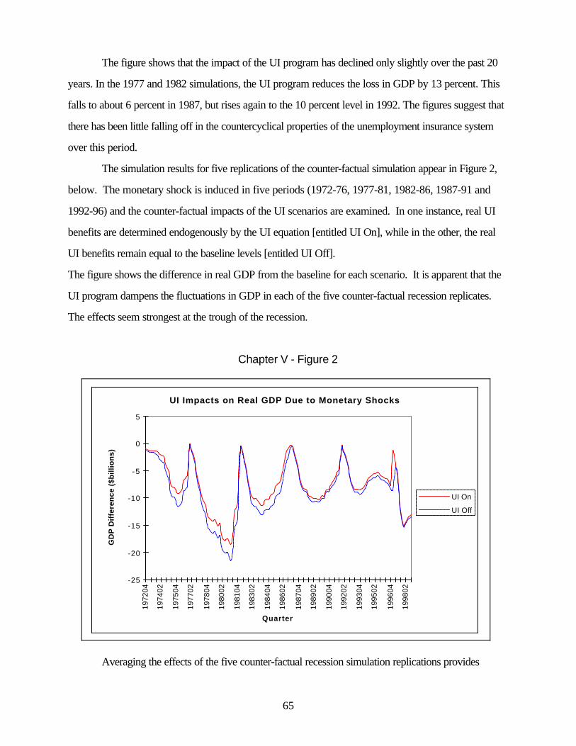
65

UI Impacts on Real GDP Due to Monetary Shocks

-25

-20

-15

-10

-5

0

5

1972

04

1974

02

1975

04

1977

02

1978

04

1980

02

1981

04

1983

02

1984

04

1986

02

1987

04

1989

02

1990

04

1992

02

1993

04

1995

02

1996

04

1998

02

Quarter

GD

P D

iffe

ren

ce (

$bill

ion

s)

UI On

UI Off

The figure shows that the impact of the UI program has declined only slightly over the past 20

years. In the 1977 and 1982 simulations, the UI program reduces the loss in GDP by 13 percent. This

falls to about 6 percent in 1987, but rises again to the 10 percent level in 1992. The figures suggest that

there has been little falling off in the countercyclical properties of the unemployment insurance system

over this period.

The simulation results for five replications of the counter-factual simulation appear in Figure 2,

below. The monetary shock is induced in five periods (1972-76, 1977-81, 1982-86, 1987-91 and

1992-96) and the counter-factual impacts of the UI scenarios are examined. In one instance, real UI

benefits are determined endogenously by the UI equation [entitled UI On], while in the other, the real

UI benefits remain equal to the baseline levels [entitled UI Off].

The figure shows the difference in real GDP from the baseline for each scenario. It is apparent that the

UI program dampens the fluctuations in GDP in each of the five counter-factual recession replicates.

The effects seem strongest at the trough of the recession.

Chapter V - Figure 2

Averaging the effects of the five counter-factual recession simulation replications provides

66

Average Difference In Real GDP from Baseline

-12.00

-10.00

-8.00

-6.00

-4.00

-2.00

0.00

1 2 3 4 5 6 7 8 9 10 11 12 13 14 15 16 17 18 19 20

Elapsed Quarter from Monetary Shock

GD

P D

Iffe

ren

ce ($

Bill

ion

s)

UI On

UI Off

another view of the impacts. The average impact of the five replicates appears in Figure 3 (p. 65)

below. The figure shows that the UI program offsets the decline in real GDP throughout the 20

quarters of real GDP decline induced by the monetary shock (the 2 percent decline in non-borrowed

reserves continues during the entire simulation).

After 15 quarters, the economy begins to recover in each scenario. Each counter-factual

simulation replicate ends after five years and is replaced by the next replicate. As the figure shows, the

decline in real GDP is reversed as recovery begins.

The percentage of real GDP loss offset by the UI program in each of the five counter-factual

scenario replicates is shown in Figure 3. Differences in the business cycle adjustments to the monetary

shock result in the different paths of recovery shown in the graph.

Chapter V - Figure 3

The average percentage of real GDP offset by the UI program appears in Figure 4 (p. 66) below.

The impacts of the monetary shock take five quarters to fully take effect and the economy’s recovery

adjustments occur over a longer period. Hence, the measurement of the full impacts might best be assessed

over the entire simulation period.

67

Percent of Simulated GDP Recession Loss Offset by UI: Average of All Monetary Shock Scenario Replicates

0%

5%

10%

15%

20%

25%

30%

35%

1 2 3 4 5 6 7 8 9 10 11 12 13 14 15 16 17 18 19 20

Elapsed Quarters from Monetary Shock

Per

cent

Chapter V – Figure 4

Over all five counter-factual simulation replicates, UI expenditures offset an average of about 15

percent of the change in real GDP. Using an unweighted average of each quarter, the UI program offset

16.43 percent of the loss in real GDP over the five periods; the weighted average offset (adjusts for

changes in UI and the economy since the 1970s) is 13.21 percent of real GDP.

Multipliers

The income expansion multipliers for each of the monetary shock experiment’s simulation replicates

appear in Table 3 (p. 67), below. During each of the counter-factual simulations, the impact of the UI

program leads to a significant countercyclical effect on real GDP. The average multiplier is 2.15 and ranges

from 1.54 to 3.07. This means that each UI benefit dollar going to a claimant ultimately expands overall

68

GDP by between $1.54 and $3.07. The average growth in overall GDP generated by a dollar of UI

benefits is $2.15.

Chapter V – Table 3

Income Expansion Multipliers and Job Impacts

Multiplier Summary Unadjusted Jobs

1972-76 3.07 4.13 150,3851977-81 1.78 2.33 205,2761982-86 2.38 7.06 122,8521987-91 1.65 2.57 47,7471992-96 2.48 2.92 47,9211997-01 1.54 2.39Average 2.15 3.56 131,565

The multiplier values are quite sensitive to the number of time periods included in the simulation

episode. If three of the outlier quarters are excluded from the measure, the volatility of the multipliers is

dramatically reduced. Since the simulation replicates are phased in over several quarters, most of these

outlier quarters occur during the phase-in of the monetary shock and it is probably best to exclude

them.

The adjusted values of the multipliers appear in the first column, while the unadjusted multipliers

appear in the second column. Using these multipliers as empirical proxy measures for the

countercyclical effectiveness of the UI program, the recession of the 1990s appeared to have had the

most effective impacts since the recession of the 1970s. However, the dynamic stability of the model

and the architecture of the simulation scenarios may be causing unintended effects and this issue is the

subject of future research.

The jobs impact also appears in Table 3. The average peak annual job savings during a recession

replicate is 131,000. However, there is significant variance and the jobs impact appears to have declined

69

in the 1980s and flattened out in the 1990s.

Current Recession Simulation

A “what-if” simulation was run to determine the importance of the unemployment insurance system

in a recession under current conditions. The exercise is based on WEFA’s global recession scenario from

November 1998. This scenario, used for planning purposes by WEFA’s corporate subscribers, assumes

that foreign economies slow considerably in 1999 and that the U.S. economy suffers from a significant

recession because of the foreign slowdown. As a result of the recession, unemployment insurance payments

in 1992 dollars jump to about $40 billion from $18 billion at the end of 1998.

The simulation used the same recession assumptions, but assumed that unemployment insurance

payments grew only at the rate of inflation to create a second recession scenario. Table 4, below,

compares the difference in real GDP between the WEFA recession (with the UI program) and the

scenario without the UI program. The table shows that by the middle of 2000, the UI program would

pump about $10 billion to $15 billion in real income into the economy, income that would not get into

the hands of consumers without the existence of the program. The impact on GDP is delayed somewhat

(because of the lag between the receipt of income and its impact on spending in the model). However,

by 2001, the additional $25 billion in UI benefits payments raises GDP significantly.

Chapter V – Table 4

GDP and Real UI Benefit ImpactWEFA Recession vs. No UI Program Scenario

UI Benefit Payments Ratio, GDP to UI

Quarter GDP Difference Difference Benefits1999 Q1 0.0 (0.1) 0.1

1999 Q2 (0.1) (0.4) 0.2 1999 Q3 (0.3) (1.2) 0.2 1999 Q4 (0.7) (3.0) 0.2 2000 Q1 (1.5) (5.9) 0.3 2000 Q2 (2.8) (10.2) 0.3 2000 Q3 (4.5) (15.3) 0.3 2000 Q4 (6.4) (20.3) 0.3 2001 Q1 (8.1) (23.9) 0.3 2001 Q2 (9.3) (25.1) 0.4 2001 Q3 (9.9) (23.8) 0.4

70

2001 Q4 (10.1) (20.7) 0.5

However, the current study focuses on the total macro-economic stimulus represented by all UI

expenditures during recessions (including UI’s extended and supplemental benefits programs as well as its

regular benefits program). To assess that overall stimulus, the current study analyzes for the first time the

aggregate economic impact of all three tiers of UI benefits (regular, extended, and supplemental), as well

as the individual economic stimuli provided by the supplemental benefits programs enacted during the last

three recessions. There were major discontinuities in the historical data on extended benefits in the Metrica

data sets, and the study did not include data on the supplemental UI programs.

In addition, the two studies used different econometric models, with different structures and inherent

multipliers, although it is difficult to quantify the precise effects of these factors. Part of the difference also

may be explained by the fact that Metrica measured UI’s cushioning effect based on one data point during

each recession. The current study uses an average of data points over time, considering that a more

effective approach. The findings of this study are in fact more consistent with the findings of prior analyses

-- for example, those of von Furstenburg (1976), de Leeuw, et al (1980), and McGibany (1983).

Other differences between the two studies include the economic specification for the benefit

equation used in the simulations, the use of GNP in Metrica and GDP in the current study, and the fact that

more timely and complete data sets were available for the current study.

Other Absolute Measures of the Effectiveness of UI

The WEFA model demonstrates the dynamics of UI’s economic stabilization role within the macro-

economy over time. The fundamentals of this macro-economic model may also be described by a single

descriptive equation that relates the UI stimulus to fluctuations in GDP. This measures UI effectiveness in

absolute terms by measuring its impact on changes in GDP in percentage terms.

Chapter V - Figure 5

71

Net UI vs. Delta GDP [lagged 3 quarters]

-15,000,000-10,000,000-5,000,000

05,000,000

10,000,00015,000,00020,000,00025,000,00030,000,000

12/3

1/71

9/30

/73

6/30

/75

3/31

/77

12/3

1/78

9/30

/80

6/30

/82

3/31

/84

12/3

1/85

9/30

/87

6/30

/89

3/31

/91

12/3

1/92

9/30

/94

6/30

/96

3/31

/98

Quarter

$100

0 Net UI

Delta GDP

The role of UI as an automatic stabilizer is visualized in Figure 5, above. For the purposes of the analyses

here and in Chapter VI, a UI characteristic called “Net UI” is applied. Net UI in this study always refers

to total UI benefits (regular, extended, and supplemental) less employer-paid UI taxes. Recent levels of

Net UI financial flows may be compared to changes in GDP during three recessions in the 1970s, 1980s

and 1990s. Both measures are four-quarter moving averages presented in real 1992 dollars per quarter,

with GDP lagged three quarters. A four-quarter moving average (using the prior four quarters) is adopted

to adjust for seasonal fluctuations that could distort the underlying economic parameters. The phase

adjustments in GDP (three-quarter lag) are made in this analysis because the single equation specification

requires a contemporaneous relationship between the right-hand-side and the left-hand-side variables.

Figure 5 clearly demonstrates that there is a difference between the peaks of Net UI and the troughs of

changes in GDP. Countercyclical impacts of UI are obvious: Net UI flows peak during recessions and

999999999 To illustrate the delta GDP variable, suppose GDP is $8 trillion annually, or about $2 trillion quarterly. If a recession ofextraordinary severity were to lead to a 2 percent reduction in GDP per quarter, this would amount to a $40-billion quarterly decline inGDP (Delta GDP= -$40 billion). For comparison, at the peak of the 1990’s recession, the second quarter of 1992, annualized UI benefitexpenditures exceeded $40 billion.

72

decline during booms. 999999999

In Figure 5, the magnitude of the difference in the change in GDP from peak to trough is measured

in each of the last three recessions. For example, in the 1970s the magnitude of the peak-to-trough

difference in the change in GDP is $24.65 billion. Delta GDP is te first difference in the four-quarter

moving average.

Chapter V – Table 5

Ratio of Change in Net UI to Change in GDP

Recession Peak to Trough Change ($Billions) Net UI UI Benefits

Net UI Delta GDP UI Benefits Ratio Ratio

1970’s 7.69 24.65 7.50 0.3119 0.30411980’s 7.11 21.59 7.52 0.3291 0.34831990’s 6.9 20.64 7.28 0.3345 0.3529

Quantification of these patterns may be seen in Table 5, above, which presents the ratio of the

change in Net UI (from peak to trough) to the change in GDP (from peak to trough) in the last three

recessions. The Net UI ratio is an empirical measure defining the relationship between the severity of GDP

downturns and Net UI program financial expenditures (macro-economic countercyclical stimulus). (Net

UI ratio = peak-to-trough change in Net UI expenditures/peak-to-trough fluctuation in the change in real

GDP.) Net UI is not first-differenced, since it already represents a change in fiscal spending.

The data in the table show that in the 1970s, the peak-to-trough change in Net UI payments totaled

$7.69 billion -- representing 31.19 percent of the magnitude of the peak-to-trough difference in the change

in GDP. In the 1980s this ratio increased to 32.91 percent, and in the 1990s the ratio increased slightly

to 33.45 percent. Table 5 also shows the same ratios for UI benefits alone, with the same patterns

emerging. Despite the measure’s crudeness, the ratios suggest that over the three recessionary periods

examined, the Net UI countercyclical stimulus may have played a growing role in mitigating the severity of

73

GDP downward fluctuations.

This peak-to-trough ratio is descriptive -- based on the visualization of the countercyclical patterns

in Figure 5. The ratio does not offer any consistent, rigorous, conceptual measure of effectiveness. It is a

quantitative counterpart of the correlation depicted in the graph, but does not provide any assessment of

the countercyclical impacts of UI relative to changes in GDP.

A Descriptive Equation for the Absolute Measure of UI Effectiveness

To determine the statistical significance of the effectiveness of UI using the absolute measures

discussed above, a descriptive equation is established that estimates the level of Net UI (total UI benefits

less employer-paid taxes). The equation [1], below, describes Net UI expenditures controlling for changes

in GDP, and includes right-hand-side dummy variables for each of the three supplemental UI programs

enacted since the 1970s. It shows how Net UI responds to changes in GDP and the effects of the

supplemental programs during recessions. The equation is estimated using quarterly data from 1971 through

the last quarter of 1998:

NetUI = a + b * Delta_GDP + c1 * D_FSB + c2 * D_FSC + c3 * D_EUC [1]

1.94 -.170 3.33 .940 3.14

(9.22) (10.99) (9.35) (3.24) (9.06) (t- statistics)

R2 = .79 F=91 df=100

where: NetUI = UI benefits – employer-paid UI taxes

four-quarter moving average

Delta_GDP = changes in real GDP (annual four-quarter moving

average, lagged three quarters)

D_FSB = Dummy variable measuring the impact of FSB

= 1 if FSB supplemental funding in effect; 0 otherwise.

D_FSC = Dummy variable measuring the impact of FSC

74

= 1 if FSC supplemental funding in effect; 0 otherwise.

D_EUC = Dummy variable measuring the impact of EUC

= 1 if EUC supplemental funding in effect; 0 otherwise.

The results are robust. Every coefficient is significant and has the expected sign. The coefficient

on the change in GDP is -.170, suggesting that over the period examined, on average, every one dollar

quarterly movement in the change in GDP was associated with a quarterly movement of 17 cents in the UI

program (benefits less taxes) in the opposite direction. Further, during the quarters they were operative,

the FSB program added net outlays of $3.33 billion, the FSC program $0.94 billion, and the EUC program

$3.14 billion each quarter. (The values in parentheses under the coefficients are t- statistics.) The

coefficients of each of the supplemental programs suggest that the effectiveness of the UI program declined

in the 1980s -- relative to the 1970s -- but exhibited an increase in effectiveness in the 1990s, at least in

terms of expenditure levels (controlling for changes in GDP).

These results are descriptive only; they do not provide the theoretical rigor of the simulation model.

Nor is the relationship depicted a proxy for the percentage decline in GDP (cited in Ch. IV – Table 1).

Rather, these results show UI’s performance relative to the pace and depth of GDP decline -- that is, the

severity of a recession. But they use real rather than simulated data and are quantitative counterparts of

the visual evidence presented in the preceding graph.

While the simulations and the equation represent wholly separate tests of UI’s effectiveness as a

stabilizer, it is notable that the equation’s results are statistically significant as well as surprisingly similar to

the results of the simulations. That is, the coefficient on Delta GDP is similar to the results obtained in the

simulations.

Permanent and Temporary UI Programs: Regular, Extended and Supplemental

If the permanent and temporary UI programs have similar effectiveness, a dollar of regular benefits

should have economic impacts similar to those of a dollar of extended or supplemental benefits.

This analysis examines the permanent and temporary UI programs separately to see what

similarities and differences exist with regard to their impact on the economy. The equation used in the

WEFA econometric simulation model provides a specification to estimate separate equations for each of

the UI programs. This equation provides measures of each program’s effectiveness and the statistical

significance of parameters for tests of hypotheses about the similarities and differences among the programs.

75

Empirical Evidence about the Permanent and Temporary UI Programs

This approach to the empirical analysis of the UI model uses a form of the UI equation from the

econometric model used for the counter-factual (what-if) simulations. The labor equation for the whole

program in the larger econometric model provides a convenient template to model each component of the

permanent and temporary UI programs (Regular, Extended, and Supplemental).

The labor equation shows that:

B* = a0 * IU b0 [2]

where: B* = real UI benefits

IU = proxy for the number of insured unemployed

IU = U * (TW/W)

U = total unemployed

TW = taxable wages

W = total wages.

a0 = constant term

b0 = elasticity of benefits with respect to the

number of insured unemployed

The coefficient on the number of insured unemployed [b0] is an elasticity term that describes the

responsiveness of UI benefits to changes in the level of insured unemployed. The elasticity is defined as

the percentage change in UI benefits divided by the percentage change in the number of insured

unemployed. This coefficient is significant at the 99 percent level of confidence, and is equal to .98 for the

total program, 1.00 for the regular program, 1.06 for extended benefits, and .97 for the temporary

supplemental program.

For each of the permanent and temporary UI programs, the same specification is used. The

variables U (total unemployed), TW (taxable wages), and W (total wages) are used in the equation for the

simulation model. These variables, when taken as a product term (shown in the equation as the variable

IU), represent a proxy variable for the number of insured unemployed. Since these data are not available

for the individual UI programs, the actual level of insured unemployed is used for each individual program.

A set of statistical hypotheses is specified to examine the similarities and differences between the

overall UI program and the individual program components of UI. One expects to find that the program

76

characteristics that create economic impacts are quite similar, although timing differences in their application

are anticipated. Public finance theory would suggest that a dollar of expenditure of each program leads to

similar impacts, but that the effects of each program are additive when they operate contemporaneously.

The results for the UI program labor equation and the temporary program equations appear in

Table 6 (next page). The estimators for the parameters are shown along with their t-statistics. The R2 for

each equation is also shown along with the corresponding F-statistic and the degrees of freedom. The

equation results show that each of UI’s component programs (regular, extended, and supplemental) and

the total program all exhibit the same degree of responsiveness to the level of insured unemployed.

Chapter V - Table 6

UI Equation Results

Left-Hand Side Variable

a b

Total coefficient -3.36 0.98[2-1A] t-ratio (-9.88) (42.14)

R2=0.95 F=1775.41

df=103Regular coefficient -3.62 1.00

[2-2] t-ratio (-7.66) (30.64)R2=0.90

F=938.71

77

df=103Extended coefficient -4.98 1.06

[2-3] t-ratio (-38.40) (86.37)R2=0.99

F=7459.32df=94

Supplemental coefficient -3.55 0.97[2-4] t-ratio (-14.68) (45.83)

R2=0.98F=2100.77

df=49

The estimations shown above use the level of insured unemployment on the right-hand side, instead

of the proxy variable used in the UI simulation equation. Equation [2-1A] represents the equivalent

specification, and when estimated over the same time period, the results are similar (see Appendix D, p.

101, for details).

The use of the level of insured unemployed in the equation allows for estimation of each the UI

equations for each permanent or temporary UI program.

Table 7, below, presents the results for the tests of hypotheses about the similarities and differences

of the permanent and temporary UI programs, relative to the overall program. As can be seen from the

test statistics, (F critical value of 1.25) there is no evidence at the 95 percent level of significance to suggest

the key program parameters (the exponent term “b” in equation [2]) are different. Thus, it appears that

both the permanent and temporary UI programs conform to the same specification, which explains the level

of benefits for each UI program as a function of the number of insured unemployed in that program.

Chapter V – Table 7

Coefficient Equivalence Tests

a1 = a2 a1 = a3 a1 = a4 a2 = a3 a2 = a4 a3 = a40.93 0.67 0.95 1.38 0.98 1.40

F crit. = 1.25 (98%)

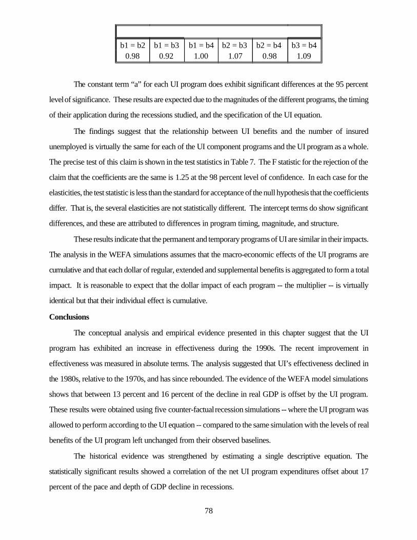
78

b1 = b2 b1 = b3 b1 = b4 b2 = b3 b2 = b4 b3 = b40.98 0.92 1.00 1.07 0.98 1.09

The constant term “a” for each UI program does exhibit significant differences at the 95 percent

level of significance. These results are expected due to the magnitudes of the different programs, the timing

of their application during the recessions studied, and the specification of the UI equation.

The findings suggest that the relationship between UI benefits and the number of insured

unemployed is virtually the same for each of the UI component programs and the UI program as a whole.

The precise test of this claim is shown in the test statistics in Table 7. The F statistic for the rejection of the

claim that the coefficients are the same is 1.25 at the 98 percent level of confidence. In each case for the

elasticities, the test statistic is less than the standard for acceptance of the null hypothesis that the coefficients

differ. That is, the several elasticities are not statistically different. The intercept terms do show significant

differences, and these are attributed to differences in program timing, magnitude, and structure.

These results indicate that the permanent and temporary programs of UI are similar in their impacts.

The analysis in the WEFA simulations assumes that the macro-economic effects of the UI programs are

cumulative and that each dollar of regular, extended and supplemental benefits is aggregated to form a total

impact. It is reasonable to expect that the dollar impact of each program -- the multiplier -- is virtually

identical but that their individual effect is cumulative.

Conclusions

The conceptual analysis and empirical evidence presented in this chapter suggest that the UI

program has exhibited an increase in effectiveness during the 1990s. The recent improvement in

effectiveness was measured in absolute terms. The analysis suggested that UI’s effectiveness declined in

the 1980s, relative to the 1970s, and has since rebounded. The evidence of the WEFA model simulations

shows that between 13 percent and 16 percent of the decline in real GDP is offset by the UI program.

These results were obtained using five counter-factual recession simulations -- where the UI program was

allowed to perform according to the UI equation -- compared to the same simulation with the levels of real

benefits of the UI program left unchanged from their observed baselines.

The historical evidence was strengthened by estimating a single descriptive equation. The

statistically significant results showed a correlation of the net UI program expenditures offset about 17

percent of the pace and depth of GDP decline in recessions.

79

In the UI program equations based on the WEFA econometric model, the regular, extended, and

supplemental UI programs were not shown to exhibit any statistically significant differences in their benefit

elasticities. The constant terms did display statistically significant differences due to the varied magnitudes

of the programs, the timing of their application, and the selection of the mathematical form of the UI

equation.

VI. EVIDENCE OF THE RELATIVE EFFECTIVENESS OF UIAS AN AUTOMATIC STABILIZER FOR THE U.S. ECONOMY

Overview

One way to look at the question of how effectively the UI program performs as a stabilizer is to

compare its economic patterns with those of another major automatic stabilizer in the U.S. economy. In

other words, if UI helps to dampen the severity of economic fluctuations, how effective is UI’s dampening

action relative to another component of the economy that is said to play a similar but even more significant

role?

The analysis presented in this chapter uses changes in Federal tax receipts (includes all forms of

Federal tax receipts) as the point of comparison. Federal tax receipts are generally understood to be one

of the economy’s primary automatic stabilizers: That is, reductions in taxation have a stimulative effect on

income and spending, while tax increases dampen economic growth. Furthermore, the heavy reliance on

80

income taxes has an automatic stabilizing effect because tax liabilities automatically go down in recessions

and rise in expansion periods. The changes in Federal tax receipts over time thus provide a baseline against

which the relative impact and effectiveness of UI benefits over the same period can be measured. This

approach follows von Furstenburg’s measurement technique, which used counterfactual simulation of full-

employment GDP to measure the impacts of the UI program with comparisons to changes in Federal tax

receipts.

In examining UI’s effectiveness relative to changes in Federal tax receipts, the analysis applies the

comparison separately to UI’s permanent and temporary programs. The permanent UI programs include

Regular Benefits (RB) and Extended Benefits (EB). The temporary programs include Federal Supplemental

Benefits (FSB) in 1974-75, Federal Supplemental Compensation (FSC) in 1982-86, and Emergency

Unemployment Compensation (EUC) in 1992-94. The analysis presents measures of the contribution of

each permanent and temporary program to the effectiveness of the entire UI program and examines the

similarities and differences between them. (The sources and method used to derive FSB levels are

explained in Appendix E, p. 100.)

A simple conceptual framework is developed to show how the importance of the UI program has

changed, and empirical evidence is presented to show how the role of the program has evolved in recent

decades relative to that of the Federal tax system. The changes in Federal tax receipts depicted in this

review may be due to changes attributed to stabilization policy, discretionary tax changes or other statutory

changes outside the scope of this study, as well as those caused by shifts in the level of economic activity.

Relative Measures of the Effectiveness of UI

The question of whether UI’s role in stabilizing the economy has changed relative to the stabilization

role played by changes in Federal tax receipts was not the principal focus of this analysis initially. But

evidence that significant change has taken place over time in the relationship of UI to Federal tax receipts

emerged during the course of the study. The evidence suggests that UI’s importance as an automatic

stabilizer in the economy is growing more pivotal rather than less so. The following discussion examines

how the importance of UI may be offset by recent factors affecting personal tax receipts, including the

progressivity of tax rates, the treatment of capital gains, and the increasing importance of Social Security

taxes.

Table 1 (p. 80) shows the changes in Federal tax receipts from peak to trough as well as changes in Net

Unemployment Insurance (Net UI) from peak to trough for three recessions in the 1970s, 1980s and

81

1990s. Net UI is the difference between UI benefits and UI employer-paid taxes. (See Appendix F, p.

102, for explanation.) The data in the table show that in the 1970s, the ratio of the peak-to-trough change

in Federal taxes to the peak-to-trough difference in the change in GDP was .427, meaning that 42.7

percent of the peak-to-trough difference in the change in GDP (see Ch. V - Figure 5, p. 70) was related

to the change in Federal tax receipts, including UI. In the 1980s this ratio increased to .557, or 55.7

percent of the peak-to-trough change in GDP, and was dramatically reduced to .202 in the 1990s.

The data in the table suggest that the effectiveness of the Federal tax system as an automatic

stabilizer in the economy has declined in recent years The decline in the Federal tax ratio in the 1990s

shows that tax receipts did not exhibit the countercyclical characteristic they had in the prior two recessions

– that is, the fiscal stimulus anticipated never materialized. Meanwhile, as the findings in Chapter V indicate,

UI’s effectiveness remained intact.

Chapter VI - Table 1

Peak-to-Trough Changes

Recession Peak to Trough Change($Billions)

Fed tax UI Bene-fits

Fedtaxes

Delta GDP UI Benefits Ratio To FedTax

1970s 10.53 24.65 7.50 0.4272 0.71181980s 12.02 21.59 7.52 0.5567 0.62561990s 4.17 20.64 7.28 0.2018 1.7489The ratio of the peak-to-trough change in UI benefits to the peak-to-trough difference in the change

in Federal tax receipts provides even more compelling evidence of the need to maintain UI as an automatic

stabilizer. In the 1970s, this ratio was .712; in the 1980s it declined to .626; and by the 1990s, it had

dramatically increased to 1.75. This means that in the 1990's recession the UI program accounted for 75

percent more fiscal stimulus than the Federal tax system -- a level of relative importance greater than any

period in the last three decades. In the 1990s, the bulk of the “heavy lifting” for automatic stabilization now

rests with the UI program, despite the long-term decline in recipiency rates (which leveled off in the 1990s).

In the next section, a theoretical or conceptual framework is presented to demonstrate the

interaction between tax receipts and automatic stabilization within the economy.

A Conceptual View of Changes in the Federal Tax System’s Effectiveness

Progressive Federal tax rates provide “built-in” automatic stabilizers that change Federal tax

82

receipts in a countercyclical fashion. During recessions, changes in Federal tax receipts decline faster than

the drop in income; during booms, they grow faster than the increase in income. This feature of Federal

tax policy provides an effective automatic stabilizer.

The Federal tax structure has changed due to a number of factors. Statutory changes, such as

those related to the declining progressivity of taxation at the upper end of the income distribution and the

treatment of capital gains, have diminished progressivity. These changes can be observed. But the purpose

of this demonstration is not to examine the determinants of tax policy changes or the merits of a debate

about Federal tax policy. Rather, the impact of the changes in Federal tax receipts represents an important

reference point to establish in relation to the overall role of Federal automatic stabilizers in the economy.

The Recent Evidence

In Figure 1 below, changes in the level of Federal tax receipts are charted along with the net

financial flows of the UI program (Net UI). The countercyclical effect of Federal tax policy is apparent

during the three recessionary periods (including a lag of three quarters). In each recession period, changes

in Federal tax receipts “spike” downward -- clearly illustrating the countercyclical effects of the Federal

tax system. The net UI injections move in the opposite direction. It is important to note that the UI

measure is an imperfect proxy for receipts: It excludes changes in state trust fund balances and ignores

borrowing from general revenue.

Chapter VI - Figure 1

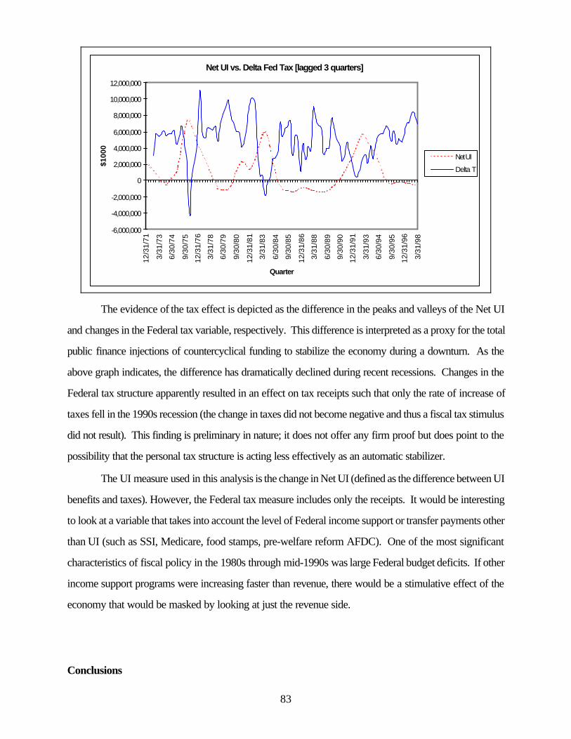
83

Net UI vs. Delta Fed Tax [lagged 3 quarters]

-6,000,000

-4,000,000

-2,000,000

0

2,000,000

4,000,000

6,000,000

8,000,000

10,000,000

12,000,000

12/3

1/71

3/31

/73

6/30

/74

9/30

/75

12/3

1/76

3/31

/78

6/30

/79

9/30

/80

12/3

1/81

3/31

/83

6/30

/84

9/30

/85

12/3

1/86

3/31

/88

6/30

/89

9/30

/90

12/3

1/91

3/31

/93

6/30

/94

9/30

/95

12/3

1/96

3/31

/98

Quarter

$100

0

Net UI

Delta T

The evidence of the tax effect is depicted as the difference in the peaks and valleys of the Net UI

and changes in the Federal tax variable, respectively. This difference is interpreted as a proxy for the total

public finance injections of countercyclical funding to stabilize the economy during a downturn. As the

above graph indicates, the difference has dramatically declined during recent recessions. Changes in the

Federal tax structure apparently resulted in an effect on tax receipts such that only the rate of increase of

taxes fell in the 1990s recession (the change in taxes did not become negative and thus a fiscal tax stimulus

did not result). This finding is preliminary in nature; it does not offer any firm proof but does point to the

possibility that the personal tax structure is acting less effectively as an automatic stabilizer.

The UI measure used in this analysis is the change in Net UI (defined as the difference between UI

benefits and taxes). However, the Federal tax measure includes only the receipts. It would be interesting

to look at a variable that takes into account the level of Federal income support or transfer payments other

than UI (such as SSI, Medicare, food stamps, pre-welfare reform AFDC). One of the most significant

characteristics of fiscal policy in the 1980s through mid-1990s was large Federal budget deficits. If other

income support programs were increasing faster than revenue, there would be a stimulative effect of the

economy that would be masked by looking at just the revenue side.

Conclusions

84

This chapter presents evidence that changes over time in the rise and fall of Federal tax receipts

may be diminishing the importance of this historically powerful automatic stabilizer in the economy. The

finding was reached by examining: (1) the increasing ratio of Net UI program benefits to changes in Federal

tax receipts, and (2) the declining proportion of fluctuations in GDP accounted for by changes in Federal

tax receipts.

By contrast, the evidence shows that, although the absolute level of UI effectiveness varies by

recession, the countercyclical action of the program as an economic stabilizer has remained consistent over

time. The declining stabilization role of Federal tax receipts suggests that UI should not be reduced but

should instead be strengthened as a stabilization mechanism during periods of economic volatility. These

findings emerged unexpectedly out of the study’s analyses. The study did not examine reasons for the

observed changes in Federal tax receipts and offers no evidence on future fluctuations. But the changing

relationship noted between UI and Federal tax receipts seems a suggestive indication of a pattern worth

examining in greater depth.

85

VII. CONCLUSIONS AND RECOMMENDATIONS

Conclusions

The findings described in this study demonstrate that the Federal-State unemployment insurance

system continues to work as an effective economic stabilizer in the U.S. economy. The UI program has

measurably and consistently mitigated the severity of downward fluctuations in GDP during economic

contractions over the last three decades.

Further, while the business cycle has been dampened over time, there is no evidence that structural

changes in the economy have eliminated the possibility of severe recessions in the future. In fact, the more

favorable business cycle pattern over the last 50 years appears, in part, to reflect the very existence of

automatic stabilizer programs. Business cycles are not a thing of the past, and neither is the need for

countercyclical forces that act automatically to stabilize the economy, particularly during periods of

economic contraction.

Highlighted, this study’s findings show that:

• The stabilizing impact of each UI benefits dollar injected into the economy has not changed

substantially over the past 25 years. Recessions -- as measured by declines in real GDP --

would be about 15 percent deeper if the UI program did not exist.

• The cushioning impact of UI during recessions results not only from the direct injection of UI

benefit dollars, but also from the spread of those dollars through the economy -- the multiplier

effect. Each dollar in UI benefits added to the economy ultimately increases overall GDP by

an average of $2.15. Moreover, because much of the multiplier effect comes after the

downturn in GDP, its result is to speed the recovery.

• Without UI, an average of 131,000 more jobs per year would be lost during recessions.

• Simulations of a future recession suggest that the effectiveness of UI in countering the downturn

in GDP will remain essentially the same.

Possible reasons for the observed improvement in UI’s performance as an economic stabilizer in

the 1990s may include the leveling off of recipiency rates, administrative changes in the management of the

UI program that improved the flow of benefit dollars, the timing of the injection of supplemental benefits

(EUC), and the nature of the recession. The study notes that the long-term downward trend in the

proportions of total unemployed and insured unemployed people who actually receive UI benefits

86

diminishes the program’s effectiveness as an automatic stabilizer. This is because declining recipiency rates

mean that fewer benefit dollars (relative to overall GDP) flow into the economy in a given economic

downturn. Although the decline appears to have halted in the 1990s, a continuation of the downward trend

would diminish the usefulness of the UI program as an automatic stabilizer in the future.

The study also notes that while the UI program’s countercyclical impact appears to be intact, a

variety of factors have changed over the time period studied. Some of these directly affect how the

program operates and others affect the larger economy.

Most surprising among these factors is the declining role of changes in federal tax receipts as an

automatic stabilizer. Historically viewed as one of the most powerful automatic stabilizers in the U.S.

economy, federal tax receipts are shown in this study to be playing a diminishing role in dampening cyclical

fluctuations in GDP. The UI program, by contrast, is shown to play a consistent stabilization role over time.

Consequently, the study concludes, the UI program has become even more important, and is probably one

of the most effective automatic stabilizers available in the economy to dampen the severity of downturns

in GDP. Recent cutbacks and changes in the federal welfare and food-stamp programs have probably

diminished the effectiveness of these programs as automatic stabilizers as well, further increasing the need

to maintain an effective unemployment insurance program.

The study also cites the imperfect automaticity of UI -- that is, key components (the temporary

supplemental programs) of UI are activated only by acts of Congress, and others depend on state

lawmaking -- and structural problems in the adequacy of financing for the Federal-State UI partnership as

issues that could also limit the effectiveness of UI as an economic stabilizer in the future.

But despite the limitations imposed on UI by these factors, the authors of this study conclude that the

program plays a significant, and now almost singular, macro-economic role in stabilizing the U.S. economy

during periods of volatility.

Recommendations

The authors recommend that UI be strengthened and improved to bolster its automatic stabilization role.

It should not be allowed to wither through lack of attention to needed policy changes. As the nation’s

eight-year economic expansion continues and the federal budget situation improves dramatically, now

would seem to be a good time to assure the long-term future of the UI program. But further analytical work

is needed to shed light on the three key problems that potentially weigh on the program’s effectiveness as

an automatic stabilizer. To make UI more effective, measures are needed to: (1) increase recipiency rates;

87

(2) make the program more fully automatic; and, (3) raise the levels of funding supporting the UI system.

The recommendations on these subjects are the following:

1) Several researchers in recent years have examined the causes and characteristics of the

declining UI recipiency rates. The next step should be to examine possible means of

expanding UI recipiency and the alternative impacts of various policy changes, utilizing this

research to the extent possible.

2) Research should be undertaken to analyze alternative economic indicators that can be used

as triggers to activate the Extended Benefits component of the UI program. The aim of this

analysis should be to illuminate disparate impacts of various indicators and to identify which

triggers make the program more automatic in the most timely manner. This would result

in shallower recessions because UI benefits would be pumped into the economy more

quickly.

3) Proposals to encourage stabilization in the UI tax structure should be advanced that enable

States and the Federal government, working together, to raise solvency rates in the UI trust

fund.

The authors also recommend that two broader avenues of research be pursued:

1) Studies of how to make job-training programs more effective in equipping unemployed

workers with the skills employers need in the contemporary economy. It is likely that

current public policies encouraging work over welfare will produce a substantial wave of

“last hired, first fired” unemployment in a future economic contraction. The more skills

workers possess, the better able they will be to survive employment volatility and the better

positioned the workforce as a whole will be to compete in the emerging global economy.

2) Further examination of automatic stabilizers generally and individually as a type of

economic influence on the macro-economy. Just as it is presumed that Federal income tax

receipts operate to reduce volatility in GDP, it is also assumed that public investments in

welfare, food stamps, and other social support programs act as automatic stabilizers. It

may be useful to analyze the functioning of all of these stabilizers over time to see whether

they continue to play an economic stabilization role, and how that role has changed as the

economy has evolved and these programs have been restructured in recent years. In

addition, policy options that will make certain that effective automatic stabilizers exist in the

88

Table A-1The WEFA Unemployment Insurance Equation

log(trpgfuib/pdcce) [A-1]

= 1.50143 * log(nun*uiwr) - 3.15239 (26.7342) (55.3887)

Sum Sq 5.8224 Std Err 0.1970 LHS Mean -1.6920 R Sq 0.8265 R Bar Sq 0.8254 F 1,150 714.718 D.W.( 1) 0.1425 D.W.( 4) 0.5740

TRPGFUIB: UNEMPLOYMENT INSURANCE PAYMENTS, $ BILLIONSPDCCE: CHAIN-WEIGHTED CONSUMPTION DEFLATOR, 1990-100NUN: NUMBER OF UNEMPLOYED, MILLIONSUIWR: PERCENTAGE OF TOTAL WAGES SUBJECT TO TAX

future should be examined.

Appendix A

The Unemployment Insurance Equation

WEFA includes an equation to account for the effects of unemployment insurance payments in its

model. The data series is defined by the Bureau of Economic Analysis in its estimation of personal income

(Federal transfer payments for unemployment insurance, NIPA table 2.1). The equation used in the model

estimated real payment of unemployment insurance based on the number of unemployed and the portion

of wages subject to the unemployment insurance tax. Table A-1, below, shows the equation.

According to the equation, an additional 1 percent rise in the number of unemployed persons will

raise real benefits payments by 1.5 percent if all wages are covered. (The average portion of wages subject

to UI tax over this period was close to 50 percent.) As the portion of wages taxed falls, the impact of the

average unemployed person on the benefits payout also falls, however.

89

Appendix B

The WEFA Model

WEFA’s Quarterly Model of the U.S. economy is a large-scale macro-econometric model of the

U.S. economy. The model reflects current macro-economics research. It has Keynesian characteristics in

the short-run, monetarist characteristics in the medium run, and operates as a neo-classical growth model

in the long run. WEFA staff has used up-to-date econometrics and economic theory to specify and estimate

the model. (See Bachman, et al [1999] for a more complete description of the model.)

Model Structure

Data embodied in the core of the U.S. Model are organized around the National Income and

Product Accounts (NIPA). These data show how the final expenditures on consumption, investment,

government, exports, and imports add up to the gross domestic product. The other side of the account is

incomes earned by type. In addition to the NIPA data, many other sets of variables are embodied, such

as data on the consumer and producer price indices, the index of industrial production, employment by

industry, etc. Conceptually, the model portrays the aggregate demand and aggregate supply of the U.S.

economy with endogenous monetary policy and exogenous fiscal policy.

Aggregate Demand

Product Markets include detailed final demand categories as published in the National Income and

Product Accounts. Money Markets include a monetary policy reaction function for the Federal funds rate,

detailed short- and long-term interest rate structure, and monetary aggregates.

Aggregate Supply

Labor market sector contains industry employment details and wage rates. Income side includes

detailed national income distribution; and household, federal, and state government income accounts. There

are several industry categories that cut across both aggregate demand and aggregate supply: agriculture,

autos, energy, and housing.

The components of final demand are modeled from the bottom up using standard approaches which

employ various measures of permanent income, output, and relative prices. Relative price variables for

investment goods incorporate the detailed cost of capital specifications, which include a variety of tax policy

90

levers such as investment tax credit, depreciation method, and corporate profit tax rate. In addition to

detailed consumption, fixed investment, and inventory sectors, the model contains fully specified housing,

auto, and energy sectors.

The model also includes a detailed trade sector in which eleven categories (nine of goods and two of

services) of both exports and imports are modeled individually. Each is related to appropriate

income/demand variables as well as to relative prices. The demand and domestic price variables in the

import equations are aligned with the corresponding final demand terms.

Industry-specific input-output weights are applied to the components of spending to construct

measures of output produced by each of the one-digit industries. These industry output variables determine

labor and capital requirements by industry. Employment, wage rates, and interest rates are key

determinants in income distribution. The price sector employs a stage-of-processing approach, which starts

with unit labor costs and other input prices to determine producer prices. Producer prices are major

determinants of the various implicit price deflators, which then finally determine the consumer price indexes.

The process is simultaneous, however, since the deflators (along with a measure of labor market tightness)

are also determinants of the key wage index via an augmented Phillips curve equation.

The model captures important linkages between the financial (LM curve) and real sectors (IS curve)

of the economy. Outcomes in the economy affect the Federal funds rate through a Federal Reserve

reaction function. Long-term interest rates are modeled as functions of short-term rates, inflation

expectations, and the federal budget deficit. In addition to their impacts on the flows of interest payments

and receipts, interest rates affect user cost of capital variables, relative prices of consumer durables, and

the consumer sentiment index, all of which influence investment and consumption.

Key fiscal policy levers, demographics, oil and food prices, inflation and growth in the rest of the

world, and seasonal patterns are exogenous variables.

Estimation Method

All stochastic or behavioral equations were estimated using ordinary least squares (OLS). While

simultaneous equation techniques are available for estimating economy-wide models, most large-scale

models are estimated using OLS. The parameters of models estimated using more advanced techniques

seldom differ very much from those produced using OLS. Re-estimating or re-specifying existing equations

or adding new equations occurs frequently enough to make simultaneous equation techniques cumbersome.

91

The model makes extensive use of error correction models (ECM’s) in the equations for aggregate

demand. This technique allows differential short- and long-term elasticities, and in many cases allows for

both more efficient estimation of the individual equations, and greater assurance that the entire model is

stable.

92

Appendix C: Simulation Results

Table C1: Impact of Monetary Policy Experiments

Monetary Contraction Beginning in 1972

Difference From Historical Baseline1972 1972 1972 1972 1973 1973 1973 1973 1974 1974 1974 1974 1975 1975 1975 1975

I II II IV I II III IV I II III IV I II III IVReal GDP, $ 1992 Billions

Monetary Contraction with UI 0.0 -0.1 -0.4 -0.9 -1.1 -1.2 -1.2 -1.3 -1.6 -2.1 -2.4 -4.1 -5.3 -7.7 -8.2 -9.1Monetary Contraction withoutUI

-0.1 -0.3 -0.6 -1.1 -1.4 -1.6 -1.6 -1.9 -2.4 -3.2 -3.6 -5.4 -6.8 -9.6 -10.0 -11.2

Unemployment Insurance Expenditures, $ MillionsMonetary Contraction with UI 2 3 8 21 32 41 45 46 62 83 103 168 239 348 401 456Monetary Contraction withoutUI

0 0 0 0 0 0 0 0 0 0 0 0 0 0 0 0

Federal Deficit, $ BillionsMonetary Contraction with UI 0.0 0.0 -0.1 -0.2 -0.2 -0.3 -0.3 -0.4 -0.6 -0.8 -0.9 -1.3 -1.6 -1.8 -2.0 -2.3Monetary Contraction withoutUI

0.0 0.0 -0.1 -0.2 -0.3 -0.3 -0.4 -0.5 -0.7 -0.9 -1.1 -1.4 -1.6 -1.7 -1.9 -2.1

Monetary Contraction Beginning in 1977Difference From Historical Baseline

1977 1977 1977 1977 1978 1978 1978 1978 1979 1979 1979 1979 1980 1980 1980 1980I II II IV I II III IV I II III IV I II III IV

Real GDP, $ 1992 BillionsMonetary Contraction with UI -0.2 -1.1 -2.8 -5.6 -7.9 -10.2 -11.2 -13.0 -13.8 -14.3 -14.0 -15.1 -14.6 -17.3 -17.7 -17.5Monetary Contraction withoutUI

-0.3 -1.4 -3.2 -6.1 -9.0 -11.4 -12.8 -14.9 -15.9 -16.4 -16.2 -17.4 -16.9 -19.6 -20.1 -20.0

Unemployment Insurance Expenditures, $ MillionsMonetary Contraction with UI 7 27 83 200 358 504 613 699 720 733 706 718 720 831 889 857Monetary Contraction withoutUI

0 0 0 0 0 0 0 0 0 0 0 0 0 0 0 0

Federal Deficit, $ BillionsMonetary Contraction with UI 0.0 -0.3 -0.7 -1.4 -2.0 -2.5 -3.0 -3.7 -4.1 -4.5 -4.7 -5.2 -5.3 -6.1 -6.2 -6.2Monetary Contraction withoutUI

-0.1 -0.4 -0.8 -1.5 -1.9 -2.4 -2.7 -3.3 -3.8 -4.1 -4.3 -4.8 -4.9 -5.5 -5.6 -5.6

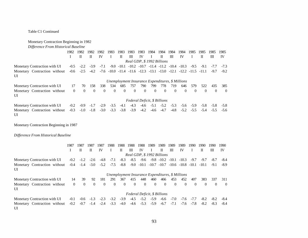
93

Table C1 Continued

Monetary Contraction Beginning in 1982Difference From Historical Baseline

1982 1982 1982 1982 1983 1983 1983 1983 1984 1984 1984 1984 1985 1985 1985 1985I II II IV I II III IV I II III IV I II III IV

Real GDP, $ 1992 BillionsMonetary Contraction with UI -0.5 -2.2 -3.9 -7.1 -9.0 -10.1 -10.2 -10.7 -11.4 -11.2 -10.4 -10.3 -9.5 -9.1 -7.7 -7.3Monetary Contraction withoutUI

-0.6 -2.5 -4.2 -7.6 -10.0 -11.4 -11.6 -12.3 -13.1 -13.0 -12.1 -12.2 -11.5 -11.1 -9.7 -9.2

Unemployment Insurance Expenditures, $ MillionsMonetary Contraction with UI 17 70 158 338 534 685 757 790 799 778 719 646 579 522 435 385Monetary Contraction withoutUI

0 0 0 0 0 0 0 0 0 0 0 0 0 0 0 0

Federal Deficit, $ BillionsMonetary Contraction with UI -0.2 -0.9 -1.7 -2.9 -3.5 -4.1 -4.3 -4.6 -5.1 -5.2 -5.3 -5.6 -5.9 -5.8 -5.8 -5.8Monetary Contraction withoutUI

-0.3 -1.0 -1.8 -3.0 -3.3 -3.8 -3.9 -4.2 -4.6 -4.7 -4.8 -5.2 -5.5 -5.4 -5.5 -5.6

Monetary Contraction Beginning in 1987

Difference From Historical Baseline

1987 1987 1987 1987 1988 1988 1988 1988 1989 1989 1989 1989 1990 1990 1990 1990I II II IV I II III IV I II III IV I II III IV

Real GDP, $ 1992 BillionsMonetary Contraction with UI -0.2 -1.2 -2.6 -4.8 -7.1 -8.3 -8.5 -9.6 -9.8 -10.2 -10.1 -10.3 -9.7 -9.7 -8.7 -8.4Monetary Contraction withoutUI

-0.4 -1.4 -3.0 -5.2 -7.5 -8.8 -9.0 -10.1 -10.7 -10.7 -10.6 -10.8 -10.1 -10.1 -9.1 -8.9

Unemployment Insurance Expenditures, $ MillionsMonetary Contraction with UI 14 39 92 181 291 367 415 448 460 466 453 452 407 383 337 311Monetary Contraction withoutUI

0 0 0 0 0 0 0 0 0 0 0 0 0 0 0 0

Federal Deficit, $ BillionsMonetary Contraction with UI -0.1 -0.6 -1.3 -2.3 -3.2 -3.9 -4.5 -5.2 -5.9 -6.6 -7.0 -7.6 -7.7 -8.2 -8.2 -8.4Monetary Contraction withoutUI

-0.2 -0.7 -1.4 -2.4 -3.3 -4.0 -4.6 -5.3 -5.9 -6.7 -7.1 -7.6 -7.8 -8.2 -8.3 -8.4

94

95

Table C1 ContinuedMonetary Contraction Beginning in 1992Difference From Historical Baseline

1992 1992 1992 1992 1993 1993 1993 1993 1994 1994 1994 1994 1995 1995 1995 1995I II II IV I II III IV I II III IV I II III IV

Real GDP, $ 1992 BillionsMonetary Contraction with UI -0.4 -1.8 -3.6 -5.8 -7.3 -8.3 -8.4 -8.5 -8.2 -7.7 -6.7 -6.2 -5.7 -5.7 -5.4 -5.8Monetary Contraction withoutUI

-0.5 -1.9 -3.8 -6.1 -7.7 -9.0 -9.0 -9.3 -9.1 -8.3 -7.2 -6.8 -6.4 -6.3 -6.0 -6.5

Unemployment Insurance Expenditures, $ MillionsMonetary Contraction with UI 20 69 151 274 394 487 517 525 495 417 333 246 184 158 134 143Monetary Contraction withoutUI

0 0 0 0 0 0 0 0 0 0 0 0 0 0 0 0

Federal Deficit, $ BillionsMonetary Contraction with UI -0.2 -1.3 -2.7 -4.2 -5.4 -6.3 -6.7 -7.1 -7.3 -7.3 -7.1 -7.1 -7.1 -7.4 -7.4 -7.7Monetary Contraction withoutUI

-0.4 -1.4 -2.8 -4.3 -5.5 -6.1 -6.5 -7.0 -7.1 -7.4 -7.2 -7.1 -7.2 -7.4 -7.5 -7.8

96

Table C2: Recessions Without Unemployment Insurance, Actual vs. Simulation

1973 Recession1973 1974 1974 1974 1974 1975 1975 1975 1975 1976 1976 1976 1976 1977 1977 1977IV I II III IV I II III IV I II III IV I II III

Real GDP, $1992 BillionsActual 3946 3907 3922 3879 3853 3800 3834 3907 3952 4044 4071 4088 4125 4176 4259 4329Without UI Program 3946 3907 3922 3878 3852 3795 3825 3894 3938 4029 4057 4074 4112 4164 4251 4325

Unemployment Insurance Payments, $ BillionsActual 4.6 5.6 6.5 6.6 8.3 13.8 18.9 19.6 18.2 17.0 15.7 15.5 14.9 14.9 12.8 11.5Without UI Program 4.4 4.5 4.6 4.8 4.9 5.0 5.0 5.1 5.2 5.3 5.3 5.4 5.5 5.6 5.7 5.8

Federal Deficit, $ BillionsActual -20 -29 39 -6 -48 -72 -48 -74 -106 -91 9 -51 -91 -75 34 -49Without UI Program -20 -28 41 -5 -45 -64 -37 -62 -95 -81 18 -42 -83 -66 42 -42

1980 Recession1980 1980 1980 1980 1981 1981 1981 1981 1982 1982 1982 1982 1983 1983 1983 1983

I II III IV I II III IV I II III IV I II III IVReal GDP, $1992 Billions

Actual 4678 4566 4561 4651 4738 4696 4752 4693 4615 4634 4611 4618 4663 4763 4849 4939Without UI Program 4678 4566 4561 4651 4738 4697 4753 4693 4615 4633 4609 4615 4659 4758 4846 4937

Unemployment Insurance Payments, $ BillionsActual 11.9 15.7 18.9 17.8 16.4 15.5 14.9 16.6 19.1 23.9 26.0 31.8 30.1 31.9 23.2 19.8Without UI Program 11.9 15.7 16.1 16.4 16.9 17.1 17.5 17.7 18.0 18.1 18.4 18.6 18.8 19.0 19.3 19.4

Federal Deficit, $ BillionsActual -108 32 -61 -134 -128 65 -34 -193 -95 -10 -145 -273 -244 -117 -148 -253Without UI Program -108 32 -59 -133 -128 64 -36 -194 -94 -5 -139 -262 -234 -106 -144 -252

97

Table C2 Continued1981 Recession

1981 1981 1982 1982 1982 1982 1983 1983 1983 1983 1984 1984 1984 1984 1985 1985III IV I II III IV I II III IV I II III IV I II

Real GDP, $1992 BillionsActual 4752 4693 4615 4634 4611 4618 4663 4763 4849 4939 5053 5133 5170 5203 5257 5283Without UI Program 4678 4566 4561 4651 4738 4697 4753 4693 4615 4633 4609 4615 4659 4758 4846 4937

Unemployment Insurance Payments, $ BillionsActual 14.9 16.6 19.1 23.9 26.0 31.8 30.1 31.9 23.2 19.8 17.1 15.6 15.0 15.7 16.7 15.8Without UI Program 11.9 15.7 16.1 16.4 16.9 17.1 17.5 17.7 18.0 18.1 18.4 18.6 18.8 19.0 19.3 19.4

Federal Deficit, $ BillionsActual -34 -193 -95 -10 -145 -273 -244 -117 -148 -253 -218 -98 -132 -286 -234 -128Without UI Program -108 32 -59 -133 -128 64 -36 -194 -94 -5 -139 -262 -234 -106 -144 -252

1990 Recession1990 1990 1990 1990 1991 1991 1991 1991 1992 1992 1992 1992 1993 1993 1993 1993

I II III IV I II III IV I II III IV I II III IVReal GDP, $1992 Billions

Actual 6142 6079 6047 6074 6090 6105 6176 6214 6261 6327 6328 6360 6393 6477 6525 6600Without UI Program 6142 6078 6046 6072 6088 6103 6171 6209 6254 6320 6322 6354 6388 6472 6521 6599

Unemployment Insurance Payments, $ BillionsActual 18.2 20.9 24.5 27.7 26.0 29.2 39.2 40.4 38.7 37.1 34.5 34.4 34.7 32.6 27.7 23.9Without UI Program 17.3 17.6 17.8 17.9 18.0 18.2 18.3 18.5 18.6 18.8 18.9 19.0 19.1 19.2 19.3 19.4

Federal Deficit, $ BillionsActual -231 -345 -262 -103 -365 -335 -462 -113 -250 -482 -249 -71 -217 -366 -235 1Without UI Program -231 -342 -256 -94 -358 -325 -444 -94 -232 -465 -235 -56 -202 -353 -225 7

98

Appendix DEstimates of Relation Between UI and the Economy

The labor equation used to evaluate the counterfactual simulations in Chapter V is used here as a

model for each UI component program. The labor equation [2], identical to the one in Chapter V, shows

that

B* = a1 * IU b1 [2]where: B* = real UI benefits

IU = proxy for the number of insured unem-ployed

IU = U * (TW/W)U = total unemployed

TW = taxable wagesW = total wages

For each of the permanent and temporary UI programs (Regular, Extended and Supplemental),

the same specification is used, but instead of a proxy for the number of insured, the actual number of

insured receiving benefits is used on the right-hand side. Thus, the system of equations estimated is:

Regular: RB* = a2 * RIU b2 [2-2]Extended: EB* = a3 * EIU b3 [2-3]Supplemental: SB* = a4 * SIU b4 [2-4]

where: RB* = real Regular benefitsRIU = number of unemployed receiving Regular

Program benefitsEB* = real Extended benefitsEIU = number of unemployed receiving

Extended Program benefits

SB* = real Supplemental benefitsSIU = number of unemployed receiving

Supplemental Program benefits

Estimates of the Contributions of UI Regular, Extended and Supplemental Benefits

The results for the UI program labor equation and the component program equations appear in

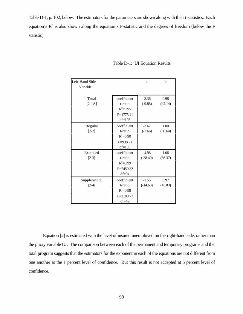
99

Table D-1, p. 102, below. The estimators for the parameters are shown along with their t-statistics. Each

equation’s R2 is also shown along the equation’s F-statistic and the degrees of freedom (below the F

statistic).

Table D-1: UI Equation Results

Left-Hand Side Variable

a b

Total coefficient -3.36 0.98[2-1A] t-ratio (-9.88) (42.14)

R2=0.95 F=1775.41

df=103

Regular coefficient -3.62 1.00[2-2] t-ratio (-7.66) (30.64)

R2=0.90F=938.71df=103

Extended coefficient -4.98 1.06[2-3] t-ratio (-38.40) (86.37)

R2=0.99F=7459.32

df=94

Supplemental coefficient -3.55 0.97[2-4] t-ratio (-14.68) (45.83)

R2=0.98F=2100.77

df=49

Equation [2] is estimated with the level of insured unemployed on the right-hand side, rather than

the proxy variable IU. The comparison between each of the permanent and temporary programs and the

total program suggests that the estimators for the exponent in each of the equations are not different from

one another at the 1 percent level of confidence. But this result is not accepted at 5 percent level of

confidence.

100

The results for the model used in Chapter V appear below:

Table D-2: Chapter V Model Equation Results

Model

proxy for IU

1962-1998

[2-1B]

coefficient

t-ratio

R2

F

-3.15

(-55.39)

0.83

714.80

1.50

(26.74)

150

Model

proxy for IU

1971-1998

[2-1C]

coefficient

t-ratio

R2

F

-4.32

(-36.21)

0.60

156.86

1.33

(12.52)

103

The results are those for the model used in Chapter V and are estimated using data for equation

[2] from 1961-1998, shown as [2-1B] in Table D-1 above. In order to have comparable results, this

equation for the total UI program is re-estimated from the period 1971-1998 and appears as [2-1C].

Examining the standard errors for the exponent terms suggests that, at the 95 percent level of significance,

the exponents of the UI component programs are within the confidence interval for the proxy form of the

UI equation.

A hypothesis is tested to examine the relation between the entire program equation and the sub-

program equations.

Test I: a1 = a2 = a3 = a4

Test II: b1 = b2 = b3 = b4

Table D-3: Coefficient Equivalence Tests

a1=a2 a1=a3 a1=a4 a2=a3 a2=a4 a3=a40.93 0.67 0.95 1.38 0.98 1.40

F crit. = 1.25 (95%)b1=b2 b1=b3 b1=b4 b2=b3 b2=b4 b3=b40.98 0.92 1.00 1.07 0.98 1.09

The evidence from simple equivalence tests for the coefficients allows us to test whether the

101

estimators are the same for each of the UI programs (Total [2-1], Regular [2-2], Extended [2-3] and

Supplemental [2-4]). The test values shown in Table D-3 are F-statistics.

The tests for equivalence are conducted at the 95 percent level of significance. The crucial

exponential term, conceptually the most important factor impacting the marginal effects and macro-

economic multipliers, is virtually identical across all equations. There is no evidence to suggest that the

estimators for these parameters are different from one another.

It is clear that the constant term “a” is significantly different across each of the UI programs. This

result is not surprising since the magnitudes of the programs differ and the equation is in the log-linear form.

Moreover, there are significant differences in the timing of the programs’ implementation and these factors

contribute to the observed differences.

102

Appendix E

Interpolation of Federal Supplemental Benefits (FSB) by Quarter

Several sources of data were used to calculate the number of FSB recipients. The FSB program

operated from the beginning of 1975 through the end of 1977. Three sources of data were available:

1) The Federal Supplemental Benefits Program, An Appraisal of Emergency Unemployment Benefits, by Walter Corson, MPR and Walter Nicholson. Table V.2 p 74

2) Extending Benefits During Recessions: Lessons From the FSB Experience, by Walter Corson and Walter Nicholson, Unemployment Compensation: Studies and Research. Table 3, p. 136

3) Key Facts: Federal Supplemental Benefits, hand-written table from USDL, ETA, UIS, ORLP, Actuarial Services August 23, 1978

Levels of FSB Recipients by Quarter

Using annual data from (3), a linear regression was developed to estimate monthly levels of weeks

compensated. The monthly estimates of weeks compensated were divided by quarterly counts of first

payments from (1) to obtain an estimate of duration (duration is estimated as an annual average equal to

the sum of weeks compensated for the past four quarters divided by the sum of first payments for the

previous four quarters).

The estimate of duration is then used to calculate the estimate for the number of FSB recipients.

The number of recipients is equal to the estimated number of weeks compensated for the quarter divided

by the annualized average duration.

103

The resulting estimates of FSB recipients are shown in Table E-1 below.

Table E-1

Estimates of FSB Participants

Summary

Quarter FSB3/31/75 435,0006/30/75 527,7749/30/75 622,24312/31/75 708,8003/31/76 791,4656/30/76 808,1449/30/76 651,13712/31/76 468,1543/31/77 357,0496/30/77 269,4969/30/77 219,95112/31/77 135,732

104

Appendix F

Estimates of Relation Between Net UI Financial Flowsand the Changes in Federal Tax Receipts

This appendix discusses some evidence about the relation between Net UI financial flows (benefits

less UI taxes) and changes in Federal tax receipts (Delta Tax) -- relative measures of the UI program’s

effectiveness (vis a vis other automatic stabilizers).

First, the historical evidence about the two variables (Net UI and changes in Federal tax receipts)

is discussed and specific measures are defined. From these two variables, a “difference” variable is

developed to determine the overall fiscal stimulus provided by Net UI and Delta Tax. Second, an

econometric equation is estimated that statistically illustrates the effectiveness of the UI program as an

automatic stabilizer in the 1990-91 recession.

Net UI Financial Flows

The difference between UI benefits and UI taxes reflects the net financial flow of resources as a

countercyclical policy instrument. UI benefits include funding for the regular UI programs, including

extended benefits, and supplemental benefits (activated by Federal legislation on a temporary basis).

UI taxes are the taxes paid by employers for covered employees. UI taxes are countercyclical ---

increasing in booms and declining in recessions. The difference between UI benefits received and UI taxes

paid is the Net UI financial flow, analyzed below.

Changes in Federal Tax Receipts

The change in Federal tax receipts is viewed as the primary source of financial flows acting as an

automatic stabilizer in the economy. During a recession, tax withdrawals from the economy (Federal tax

receipts or payments to the Federal government) decline, dampening the decline in aggregate macro-

economic expenditure. During a boom, tax withdrawals increase, dampening the inflationary increase in

macro-economic expenditure and moderating economic growth.

The “Difference” Variable: Countercyclical Macro-Economic Financial Injections

The “difference” variable is defined as Net UI benefits less the changes in Federal tax receipts

(Delta Tax). Difference is positive in a recession, indicating that Net UI benefits are positive and Federal

tax changes are negative. This means that during a recession the UI system is injecting dollars into the

economy, but so, in effect, is the Federal tax system. That is because the reductions in the overall tax bite

105

Net UI vs. Delta Fed Tax [lagged 3 quarters]

-6,000,000

-4,000,000

-2,000,000

0

2,000,000

4,000,000

6,000,000

8,000,000

10,000,000

12,000,000

12/3

1/71

3/31

/73

6/30

/74

9/30

/75

12/3

1/76

3/31

/78

6/30

/79

9/30

/80

12/3

1/81

3/31

/83

6/30

/84

9/30

/85

12/3

1/86

3/31

/88

6/30

/89

9/30

/90

12/3

1/91

3/31

/93

6/30

/94

9/30

/95

12/3

1/96

3/31

/98

Quarter

$100

0

Net UI

Delta T

that accompany recessionary times operate as a positive stimulus on the economy. Clearly, during a

recession, the larger the magnitude of these financial flows, the greater the financial injection of macro-

economic stabilizers.

Data and Adjustments

All UI data were provided by the Unemployment Insurance Service of the U.S. Department of

Labor-Employment and Training Administration. All dollar amounts are measured in real terms (using a

chain-weighted consumption deflator in 1992 dollars). Each series is taken as an annual moving average

over four quarters. The changes in Federal tax receipts are lagged three quarters to illustrate the

correspondence between these two stabilizer instruments.

Historical Evidence

The graph (Figure F-1) below illustrates the historical trend in the level of Net UI benefits and the

changes in Federal tax receipts.

Figure F-1

The historical evidence shows that Net UI and Delta Tax are closely linked as automatic stabilizers.

The gap between these two variables in the graph -- the “difference” -- appears to grow smaller, especially

during the recession in the early 1990s. The magnitude of the “difference,” or total fiscal injection into the

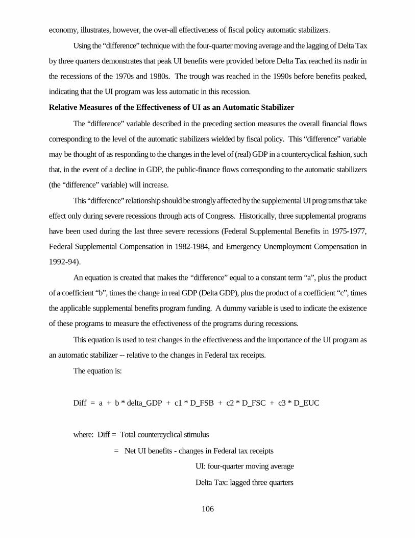
106

economy, illustrates, however, the over-all effectiveness of fiscal policy automatic stabilizers.

Using the “difference” technique with the four-quarter moving average and the lagging of Delta Tax

by three quarters demonstrates that peak UI benefits were provided before Delta Tax reached its nadir in

the recessions of the 1970s and 1980s. The trough was reached in the 1990s before benefits peaked,

indicating that the UI program was less automatic in this recession.

Relative Measures of the Effectiveness of UI as an Automatic Stabilizer

The “difference” variable described in the preceding section measures the overall financial flows

corresponding to the level of the automatic stabilizers wielded by fiscal policy. This “difference” variable

may be thought of as responding to the changes in the level of (real) GDP in a countercyclical fashion, such

that, in the event of a decline in GDP, the public-finance flows corresponding to the automatic stabilizers

(the “difference” variable) will increase.

This “difference” relationship should be strongly affected by the supplemental UI programs that take

effect only during severe recessions through acts of Congress. Historically, three supplemental programs

have been used during the last three severe recessions (Federal Supplemental Benefits in 1975-1977,

Federal Supplemental Compensation in 1982-1984, and Emergency Unemployment Compensation in

1992-94).

An equation is created that makes the “difference” equal to a constant term “a”, plus the product

of a coefficient “b”, times the change in real GDP (Delta GDP), plus the product of a coefficient “c”, times

the applicable supplemental benefits program funding. A dummy variable is used to indicate the existence

of these programs to measure the effectiveness of the programs during recessions.

This equation is used to test changes in the effectiveness and the importance of the UI program as

an automatic stabilizer -- relative to the changes in Federal tax receipts.

The equation is:

Diff = a + b * delta_GDP + c1 * D_FSB + c2 * D_FSC + c3 * D_EUC

where: Diff = Total countercyclical stimulus

= Net UI benefits - changes in Federal tax receipts

UI: four-quarter moving average

Delta Tax: lagged three quarters

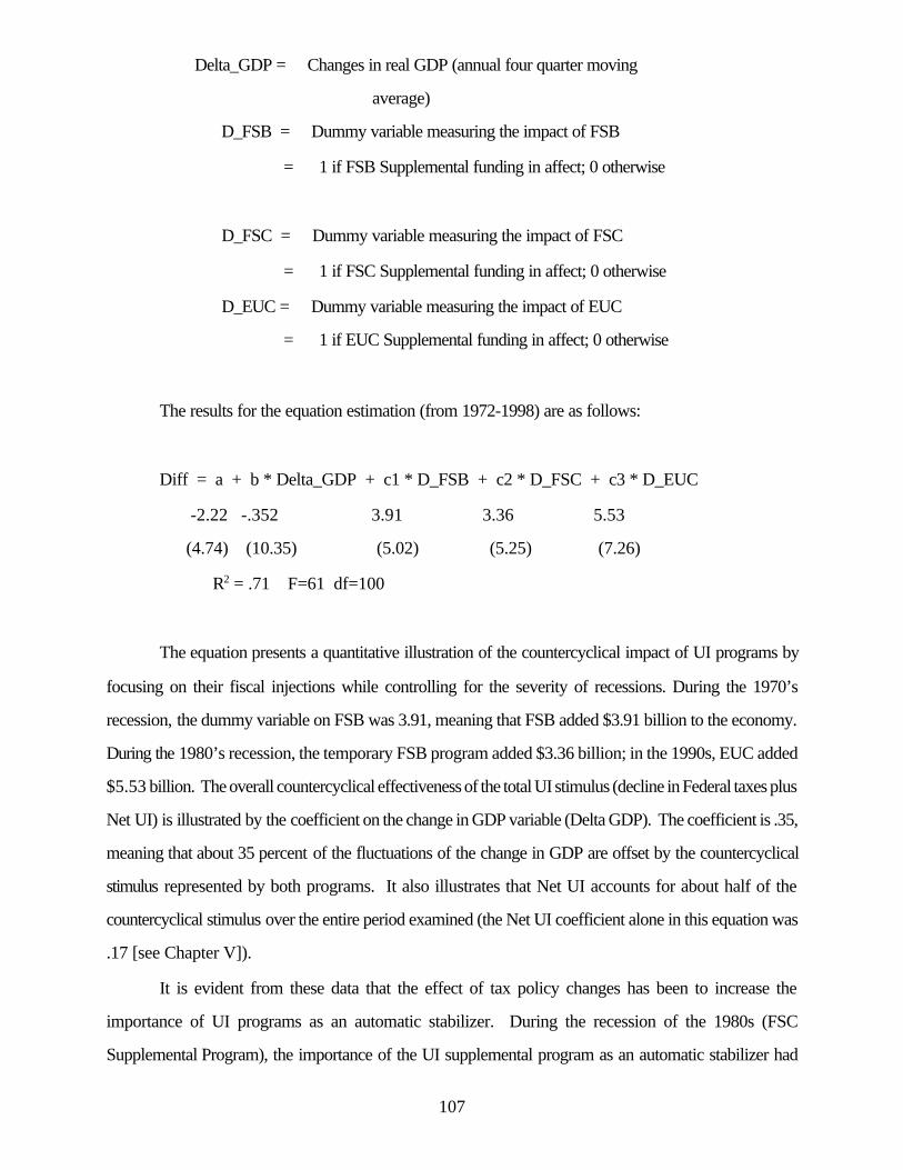
107

Delta_GDP = Changes in real GDP (annual four quarter moving

average)

D_FSB = Dummy variable measuring the impact of FSB

= 1 if FSB Supplemental funding in affect; 0 otherwise

D_FSC = Dummy variable measuring the impact of FSC

= 1 if FSC Supplemental funding in affect; 0 otherwise

D_EUC = Dummy variable measuring the impact of EUC

= 1 if EUC Supplemental funding in affect; 0 otherwise

The results for the equation estimation (from 1972-1998) are as follows:

Diff = a + b * Delta_GDP + c1 * D_FSB + c2 * D_FSC + c3 * D_EUC

-2.22 -.352 3.91 3.36 5.53

(4.74) (10.35) (5.02) (5.25) (7.26)

R2 = .71 F=61 df=100

The equation presents a quantitative illustration of the countercyclical impact of UI programs by

focusing on their fiscal injections while controlling for the severity of recessions. During the 1970’s

recession, the dummy variable on FSB was 3.91, meaning that FSB added $3.91 billion to the economy.

During the 1980’s recession, the temporary FSB program added $3.36 billion; in the 1990s, EUC added

$5.53 billion. The overall countercyclical effectiveness of the total UI stimulus (decline in Federal taxes plus

Net UI) is illustrated by the coefficient on the change in GDP variable (Delta GDP). The coefficient is .35,

meaning that about 35 percent of the fluctuations of the change in GDP are offset by the countercyclical

stimulus represented by both programs. It also illustrates that Net UI accounts for about half of the

countercyclical stimulus over the entire period examined (the Net UI coefficient alone in this equation was

.17 [see Chapter V]).

It is evident from these data that the effect of tax policy changes has been to increase the

importance of UI programs as an automatic stabilizer. During the recession of the 1980s (FSC

Supplemental Program), the importance of the UI supplemental program as an automatic stabilizer had

108

started to decline (probably due to declining recipiency). By the 1990s, the full effect of the tax policy

change is felt, increasing the coefficient of the EUC supplemental program -- indicating that the importance

of UI as an automatic stabilizer has measurably increased in the 1990s.

Appendix G

BIBLIOGRAPHY

Addison, John T. & Blackburn, McKinley L. (1997) A Puzzling Aspect of the Effect of Advance

Notice on Unemployment. Industrial and Labor Relations Review. Vol. 50, No. 2, 268-288.

Anderson, Patricia M. & Meyer, Bruce D. (August 1997) Unemployment Insurance Takeup Rates and

the After-Tax Value of Benefits. Quarterly Journal of Economics. Vol. 112, 913-937.

Anderson, Patricia M. & Meyer, Bruce D. (1995) Using a Natural Experiment to Estimate the

Effects of the Unemployment Insurance Payroll Tax on Layoffs, Employment and Wages.

Mimeo, Northwestern University.

Anderson, Patricia M. & Meyer, Bruce D. (1994) The Effect of Unemployment Insurance Taxes and

Benefits on Layoffs Using Firm and Individual Data. NBER Working Paper No. 4960.

Anderson, Patricia M. & Meyer, Bruce D. (1993) Unemployment Insurance in the United States:

Layoff Incentives and Cross Subsidies. Journal of Labor Economics. Vol. 11, No. 1.

Appelbaum, E. & Schettkat, R. (1991) Employment and Industrial Restructuring in the United States

and West Germany. Beyond Keynesianism, E. Matzner & W. Streeck (Eds.), Aldershot,

England, 137-160.

109

Atkinson, Anthony B. & Micklewright, John. (December 1991) Unemployment Compensation and

Labor Market Transitions: A Critical Review. Journal of Economic Literature 29: 1679-1727.

Bachman, et al, (1999) WEFA’s Quarterly Model. Wharton Econometric Forecasting Unit, WEFA, Inc.,

Eddystone, Pa.

Baker, Michael & Rea, Samuel A. Jr. (January 1997) Employment Spells and Unemployment

Insurance Eligibility Requirements. The Review of Economics and Statistics.

Baldwin, Marc & McHugh, Richard. (1992) Unprepared for Recession: The Erosion of State

Unemployment Insurance Coverage Fostered by Public Policy in the 1980s. Economic Policy

Institute working paper BP29.

Bassi, Laurie J. & McMurrer, Daniel P. (1997) Coverage and Recipiency. Unemployment Insurance

in the United States: Analysis of Policy Issues. W.E. Upjohn Institute for Policy Research.

Belzil, Christian. (1995) Unemployment Insurance and Unemployment Over Time: An Analysis With

Event History Data. The Review of Economics and Statistics.

Belzil, Christian. (1992) On the Empirical Relationship Between Unemployment Insurance,

Unemployment Duration and Voluntary Unemployment. Economics Letters 39, 235-240.

Bernanke, Ben & Blinder, Alan. (1992) The Federal Funds Rate and the Channels of Monetary

Transmission. American Economic Review (September), 901-921.

Black, Fisher. (1995) Exploring General Equilibrium. Cambridge: MIT Press.

Blank, Rebecca M. & Card, David E. (November 1991) Recent Trends in Insured and

Uninsured Unemployment: Is There an Explanation? Quarterly Journal of Economics. Vol.

106, No. 4, 1157-1189.

110

Blaustein, Saul J. (1993) Unemployment Insurance in the United States. W.E Upjohn Institute for

Employment Research.

Borjas, George J.; Freeman, Richard B. & Katz, Lawrence F. (1992) On the Labor Market Effects of

Immigration and Trade. Immigration and the Work Force. Chicago: University of Chicago

Press, 213-44.

Brainard, S. L. & Cutler, D. M. (1993) Sectoral Shifts and Cyclical Unemployment Reconsidered.

Quarterly Journal of Economics 108, 219-243.

Brechling, Frank P. (1995) Permanent Job Loss and the U.S. System of Financing Unemployment

Insurance. W. E. Upjohn Institute for Employment Research.

Budd, John W. & McCall, Brian P. (1997) The Effect of Unions on Receipt of Unemployment

Insurance Benefits. Industrial and Labor Relations Review forthcoming.

Burdett, Kenneth & Wright, Randall. (1989) Unemployment Insurance and Short-Time

Compensation: The Effects on Layoffs, Hours per Worker, and Wages. Journal of Political

Economy. Vol. 97, No. 6.

Burtless, Gary S. (1983) Why is Insured Unemployment So Low? Brookings Papers on

Economic Activity, 1, 225-49.

Burtless, Gary S., and Saks, Daniel. (1984) The Decline in Insured Unemployment During the 1980’s.

Washington, DC: The Brookings Institute.

Card, David & Levine, Phillip B. (January 1994) Unemployment Insurance Taxes and the Cyclical

Seasonal Properties of Unemployment. Journal of Public Economics. Vol. 53, 1-29.

111

Chesher, Andrew. (1984) Testing for Neglected Heterogeneity. Econometrica 52, 865-872.

Christiano, Lawrence J. & Harrison, Sharon G. (1996) Chaos, Sunspots, and Automatic Stabilizers.

NBER Working Paper No. 5703.

Christofides, Louis N. & McKenna, Chris J. (April 1996) Unemployment Insurance and

Employment Patterns in Canada. The Canadian Journal of Economics. Vol. 29.

Clark, Kim B. & Summers, Lawrence H. (1979) Labor Market Dynamics and Unemployment: A

Reconsideration. Brookings Papers on Economic Activity 13-60.

Clement, M. O. (1960) The Quantitative Impact of Automatic Stabilizers. Review of Economics and

Statistics 42, No. 1: 56-61.

Cochrane, John H. (1994) Shocks. NBER Working Paper No. 4698.

Corson, Walter & Decker, Paul T. (1989) The Impact of Reemployment Services on

Unemployment Insurance Benefits: Findings from the New Jersey Unemployment Insurance

Reemployment Demonstration. Unpub. Mss., Mathematica Policy Research.

Corson, Walter; Needels, Karen & Nicholson, Walter. (1998) Emergency Unemployment Compensa-

tion: The 1990’s Experience. Unemployment Insurance Occasional Paper 98-1, Washington,

DC, U.S. Department of Labor-ETA.

Corson, Walter & Nicholson, Walter. (1988) An Examination of Declining UI Claims During the

1980's. Unemployment Insurance Occasional Paper 88-3, Washington, DC; U.S. Department

of Labor-ETA.

Cremer, H.; Marchand, M. & Pestieau, P. (December 1995) The Optimal Level of

Unemployment Insurance Benefits in a Model of Employment Mismatch. (December 1995)

Labour Economics. Vol. 2, No. 4.

112

Davidson, Carl & Woodbury, Stephen A. (1997) Optimal Unemployment Insurance. Journal of Public

Economics. Vol. 74 No. 3, 359-87.

Davis, S. & Haltiwanger, J. (1992) Gross Job Creation, Gross Job Destruction, and Employment

Reallocation. Quarterly Journal of Economics 107, 819-863.

Deere, Donald R. (October 1991) Unemployment Insurance and Employment. Journal of Labor

Economics. Vol. 9, No. 4. University of Chicago.

DeLeeuw, Frank, et al. (November 1980) The High-Employment Budget: New Estimates, 1955-80.

Survey of Current Business: 13-44.

Dungan, D. Peter & Murphy, Steve. (1995) The UI System as an Automatic Stabilizer in Canada. Human

Resources Development Canada.

Dunson, Bruce, Maurice, S. Charles & Dwyer, Gerald. (1991) The Cyclical Effects of the Unemploy-

ment (UI) Program, Unemployment Insurance Occasional Paper 91-3, Washington, D.C.: U.S.

Department of Labor-ETA.

Ehrenberg, Ronald G. & Oaxaca, Ronald L. (December 1976) UI, Duration of Unemployment, and

Subsequent Wage Gain. American Economic Review 66: 754-66.

Eilbott, Peter. (1966) The Effectiveness of Automatic Stabilizers. American Economic Review 56, No.

3: 450-465.

Epstein, Gene. (1995) Economic Beat: Unemployment Insurance: Lay Off the Old, Bring in the New.

Barron’s, Vol. 75 No. 49, 44.

Erban, S.N., (1986) Inflationary Finance of Budget Deficits as an Automatic Stabilizer. Journal of

113

Monetary Economics, Vol. 18, 197-204.

Ferrall, Christopher. (1997) Unemployment Insurance Eligibility and the School-to-Work Transition

in Canada and the United States. (1997) Journal of Business and Economic Statistics, Vol. 15

No. 2, 115-29.

Fisher, Peter S. & Peters, Alan H. (1998) Industrial Incentives--Competition Among American States and

Cities. W.E. Upjohn Institute for Employment Research, Kalamazoo, Michigan.

Flinn, C. & Heckman, James. (1982) New Methods for Analyzing Structural Models of Labor Force

Dynamics. Journal of Econometrics.

Freeman, R. B. (1988) Evaluating the View That the United States Has No Unemployment

Problems. American Economic Review, 78, 294-299.

Freeman, R. B. (1988) Labor Market Institutions and Economic Performance. Economic Policy,

April, 64-80.

Green, David A. & Riddell, W. Craig. (January 1997) Qualifying for Unemployment Insurance: An

Empirical Analysis. The Economic Journal, 67-84.

Gustafson, Cynthia K. & Levine, Phillip B. (1998) Less-Skilled Workers, Welfare Reform, and the

Unemployment Insurance.

Hairault, Jean-Oliver & Henin, Pierre-Yves. (1997) Business Cycles and Macroeconomic Stability:

Should We Rebuild Built-in Stabilizers? Kluwer Academic Publishers.

Hall, Robert E. (1995) Lost Jobs. Brookings Papers on Economic Activity, No. 1, 221-256.

Han, Aaron & Hausman, Jerry. (January-March 1990) Flexible Parametric Estimation of Duration

114

and Competing Risk Models. Journal of Applied Econometrics 5: 1-28.

Hansen, Gary D. (November 1985) Indivisible Labor and the Business Cycle. Journal of Monetary

Economics 16: 309-27.

Hansen, Gary D. & Imrohoroglu, Ayse. (February 1992) The Role of Unemployment Insurance in an

Economy With Liquidity Constraints and Moral Hazard. Journal of Political Economy. Vol.

100, No. 1, 118-142.

Hasimoto, M., & Raisian, J. (1992) Aspects of Labor Market Flexibility in Japan and the United

States. Employment Security and Labor Market Flexibility, Detroit, Michigan: Wayne State

University Press, 78-101.

Hausman, Jerry. (1984) Tax Policy and Unemployment Insurance Effects on Labor Policy.

Philadelphia: University of Pennsylvania Press, 70-96.

Heckman, James & Singer, Burton. (March 1984) A Method for Minimizing the Impact of

Distributional Assumptions in Econometrics Models for Duration Data. Econometrica. 52:

271-320.

Hinde, Kevin. (November 1994) Labour Market Experiences Following Plant Closure: The Case of

Sunderland’s Shipyard Workers. Regional Studies. Vol. 28, No. 7, 713-24.

Hopenhayn, Hugo A. & Nicolini, Juan Pablo. (1997) Optimal Unemployment Insurance. Journal of

Political Economy. Vol. 105, No. 2; The University of Chicago.

Hunt, Jennifer. (January 1995) The Effect of Unemployment Compensation on Unemployment

Duration in Germany. Journal of Labor Economics. Vol. 13 No. 1, 88-120.

Janoski, T. (1990) The Political Economy of Unemployment: Active Labor Market Policy in West

115

Germany and the United States. Berkeley, California: University of California Press.

Karanassou, Marika & Snower, Dennis J. (1995) A Contribution to Unemployment Dynamics. Centre

for Economic Policy Research, Discussion Paper 1176.

Katz, Lawrence F. & Meyer, Bruce D. (February 1990) The Impact of the Potential Duration of

Unemployment Benefits on the Duration of Unemployment. Journal of Public Economics.

Vol. 41, No. 1, 45-72.

Katz, Lawrence F. & Meyer, Bruce D. (November 1990) Unemployment Insurance, Recall

Expectations, and Unemployment Outcomes. Quarterly Journal of Economics. 105(4), 973-

1002.

Kelly, A. (1997) The Performance of Illinois’ Unemployment Insurance System Over Business

Cycles. International Journal of Public Administration. Vol. 20, No. 8/9.

Lancaster, Tony. (July 1979) Econometrics Methods for the Duration of Unemployment.

Econometrica. 47: 939-56.

Larson, Tom & Ong, Paul M. (March 1994) Imbalance in Part-time Employment . Journal of

Economic Issues. Vol. 28 No. 1, 187-196.

Levin-Waldman, Oren (1997) Unemployment Insurance for a New Age; Reform of the

Unemployment Insurance System. Jerome Levy Economics Institute of Bard College, Vol. 40,

No. 2.

Levin-Waldman, Oren. (1996) Making Unemployment Insurance Work: Reforming

Unemployment Insurance: Toward Greater Employment. Annandale on Hudson: Jerome Levy

Economics Institute of Bard College. Public Policy Brief: Vol. 26.

116

Levin-Waldman, Oren. (April 1995) The Deficiencies of the Unemployment Insurance System: What

Are the Alternatives? Working Paper No. 140. The Jerome Levy Economics Institute.

Levine, P. (1993) Spillover Effects Between the Insured and Uninsured Unemployed. Industrialand

Labor Relations Review 47, 73-86.

Levine, Philip B. (1994) Unemployment Insurance Taxes and the Cyclical Seasonal Properties of

Unemployment. Journal of Public Economics. Vol. 53, No. 1.

Levine, Philip B. (1997) Financing Benefit Payments. Unemployment Insurance in the United States:

Analysis of Policy Issues. W.E. Upjohn Institute for Policy Research.

Loungani, Prakash & Trehan, Bharat. (1997) Explaining Unemployment: Sectoral vs. Aggregate

Shocks. FRBSF Economic Review. No. 1, 3-15.

MaCoy, Ramelle & Morand, Martin J. (1984) Work Sharing and Short-Time Compensation: An

Overview in Short-Time Compensation: A Formula for Work Sharing. New York: Pergamon.

Mandy, David M. (1989) Forecasting Unemployment Insurance Trust Funds: The Case of

Tennessee. International Journal of Forecasting. Vol. 5, No. 3.

Maranville, Deborah. (1995) Changing Economy, Changing Lives: Unemployment Insurance and

the Contingent Workforce. The Boston University Public Interest Law Journal. Vol. 4, No. 2.

Marceau, Nicolas. (September 1993) Unemployment Insurance and Market Structure. Journal of

Public Economics. Vol. 52, No. 2.

McCall, Brian. (April 1995) The Impact of Unemployment-Insurance Benefit Levels on

Recipiency. Journal of Business and Economic Statistics 12, 189-198.

117

McCall, Brian. (May 1996) Unemployment Insurance Rules, Joblessness, and Part-Time Work.

Econometrica. Vol. 64, No. 3, 647-682.

McGibany, James M. (1983) An Econometric Analysis of the Stabilization Effectiveness of the

Unemployment Insurance Program. University Microfilms International, 300 N. Zeeb Road,

Ann Arbor, MI 48106.

Meyer, Bruce D. (March 1995) Lessons from the U. S. Unemployment Insurance Experiments.

Journal of Economic Literature. Vol. 33, No. 1.

Meyer, Bruce D. (Winter 1995/6) The Economic Effects of Unemployment Insurance. NBER

Reporter.

Meyer, Bruce D. & Rosenbau, Dan T. (January 1996) Repeat Use of Unemployment Insurance.

National Bureau of Economic Research, NBER Working Paper Series 5423.

Milbourne, Ross D.; Purvis, Douglas D.; & Scoones, W. David. (November 1991)

Unemployment Insurance and Unemployment Dynamics. The Canadian Journal of Economics.

Vol. 24, No. 4.

Miller, Mike, Pavosevich, Robert, & Vroman, Wayne. (1997) Trends in Unemployment Benefit

Financing. Unemployment Insurance in the United States: Analysis of Policy Issues. W.E.

Upjohn Institute for Policy Research.

Mortensen, Dale T. (December 1970) Job Search, the Duration of Unemployment, and the Phillips

Curve. American Economic Review 60: 847-62.

Narendranathan, Wiji & Stewart, Mark B. (1993) How Does the Benefit Effect Vary as

Unemployment Spells Lengthen? Journal of Applied Econometrics 8, 361-381.

118

Neal, D. (1995) Industry-Specific Human Capital: Evidence from Displaced Workers. Journal of

Labor Economics 13, 653-677.

Palley, Thomas I. The Forces Making for an Economic Collapse. The Atlantic Monthly, July,

1996, Volume 278, No. 1, 44-58.

Palumbi, John R. (April 1994) The Business Economist at Work: An Unemployment Insurance

Actuary. Business Economics. Vol. 29 No. 2, 53-56.

Phelps, E. S. (1992) A Review of Unemployment. Journal of Economic Literature. Vol. XXX, 1476-

1490.

Poirier, Dale J. (1976) The Econometrics of Structural Change. Amsterdam: North Holland Publishing.

Portugal, Pedro & Addison, John. (April 1990) Problems of Sample Construction in Studies of the

Effects of Unemployment Insurance on Unemployment Duration. Industrial and Labor

Relations Review 43: 463-77.

Poterba, James M. & Summers, Lawrence H. (May 1995) Unemployment Benefits and Labor Market

Transitions: A Multinomial Logic Model With Errors in Classification. Review of Economics

and Statistics. Vol. 77 No. 2, 207-216.

Prescott, Edward C. (Fall 1986) Theory Ahead of Business Cycle Measurement. Federal Reserve

Bank Minneapolis Quarterly Review 10: 9-22.

Reissert, B. (1993) The Regional Impact of Unemployment Insurance and Active Labor Market

Policy--An International Comparison. Creating Economic Opportunities: The Role of Labour

Standards in Industrial Restructuring. Geneva: ILO Publications, 117-136.

Runner, Diana (January 1991-98) Changes in Unemployment Insurance Legislation. Monthly Labor

119

Review.

Schmid, Gunther. (Spring 1995) Institutional Incentives to Prevent Unemployment:

Unemployment Insurance and Active Labor Market Policy in a Comparative Perspective.

The Journal of Socio-Economics. Vol. 24, No. 1, 51-103.

Schmid, Gunther. (1992) Unemployment Insurance and Active Labor Market Policy: An International

Comparison of Financing Systems. Detroit: Wayne State University Press.

Schubert, Walt. (1989) Unemployment Insurance Costs: Issues and Dilemmas. International Journal

of Social Economics 16,8: 60-67.

Shin, Kwanho. (1997) Sectoral Shocks and Movement Costs: Effects on Employment and Welfare.

Journal of Economic Dynamics and Control. Vol. 21 No. 2, 3, 449-471.

Smyth, D.J. (August 1966) Built-In Flexibility of Taxation and Automatic Stabilization. Journal of

Political Economy.

Snower, Dennis J. & de la Dehessa, Guillermo. (1997) Unemployment Policy: Government Options for

the Labour Market. Cambridge; New York and Melbourne: Cambridge University Press.

Solon, Gary. (1984) The Effects of Unemployment Insurance Eligibility Rules on Job Quitting

Behavior. Journal of Human Resources 19, 118-125.

Solow, R. M. (1990) The Labor Market as a Social Institution. Oxford, England: Basil Blackwell.

Stokes, Ernie. (1995) Canada’s Unemployment Insurance Program as an Economic Stabilizer.

Human Resources Development Canada.

Tannenwald, Robert & O’Leary, Christopher J. (May/June 1997) Unemployment Insurance Policy in

120

New England: Background and Issues. New England Economic Review, 3-22.

Thomas, Jonathan. (1996) An Empirical Model of Sectoral Movements by Unemployed Workers.

Journal of Labor Economics (January), 126-153.

Topel, Robert H. (1990) Financing Unemployment Insurance: History, Incentive, Reform.

Unemployment Insurance. Madison: University of Wisconsin Press.

Tullock, Gordon. (1997) Economics of Income Redistribution. Kluwer Academic Publishers.

Uri, Noel D., Mixon, J. Wilson & Kyer, Ben L. Automatic Stabilizers Reconsidered. (1989) Public

Finance, Vol. 44, No. 3, 476, Finances Publiques.

U.S. Department of Labor, Bureau of Labor Statistics, Labstat Data Base accessible through the internet

at http://stats.bls.gov.

von Furstenberg, George M. (April 1976) Stabilization Characteristics of Unemployment Insurance.

Industrial and Labor Relations Review 29: 363-76.

Vroman, Wayne. (1986) The Funding Crisis in State Unemployment Insurance. W. E. Upjohn Institute

for Employment Research.

Vroman, Wayne. (1990) Unemployment Insurance Trust Fund Adequacy in the 1990’s. W.E. Upjohn

Institute for Employment Research.

Vroman, Wayne. (1998) Labor Market Changes and Unemployment Insurance Benefit Availability.

Report prepared for the U.S. Department of Labor under Contract No. F-5532-5-00-80-30.

Wang, Cheng & Williamson, Stephen D. (1996) Unemployment Insurance With Moral Hazard in a

Dynamic Economy. Carnegie-Rochester Conference Series on Public Policy; vol. 44, 1-41.

121

Washington Post editorial. (February 5, 1997) Protecting the Jobless.

Weber, Steven. (July 1997) The End of the Business Cycle? Foreign Affairs, Vol. 76 No. 4, 65-82.

West, Thomas E. & Hildebrand, Gerard. (1997) Federal-State Relations. Unemployment Insurance in

the United States: Analysis of Policy Issues. W.E. Upjohn Institute for Policy Research.

Wunnava, P.V. & Mehdi, S.A.R. (July 1994) The Effect of Unemployment Insurance on Unemploy-

ment Rate and Average Duration: Evidence from Pooled Cross-Sectional Time-Series Data.

Applied Economics Letters. Vol. 1, No. 7.

122

Appendix H

Glossary of Terms

Automatic stabilizer

An economic stabilizer is a fiscal or monetary instrument that acts on the economy to lessenfluctuations in the level of economic activity. A stabilizer is considered automatic if its action on theeconomy occurs without requiring external regulatory or policymaking interventions. The rise and fall ofincome-tax receipts, for example, occur automatically in relation to the rise and fall of income.

CountercyclicalAn economic stabilizer is countercyclical if its action on the economy moves in the opposite

direction from that of overall economic activity. The UI system is countercyclical because unemploy-ment benefits inject dollars into the economy at a time when economic activity as a whole is contracting,thus mitigating the severity of the economic contraction. Tax receipts, on the other hand, are anautomatic stabilizer but are not countercyclical – when the economy is contracting, the level of taxreceipts also contracts, moving in the same direction as overall economic activity.

Counter-factual

Counter-factual means contrary to the actual case, a hypothetical or “what if” formulation. In thisstudy, counter-factual scenarios are established to examine what would happen to the economy if ahypothetical state of recession were induced and the UI system were not allowed to respond as it doesordinarily. In other scenarios, UI is allowed to respond to the induced recession. These “what if” counter-factual simulations make it possible to demonstrate the dynamics of macro-economic forces without havingto experience them in reality.

Dummy variable

A dummy variable is an artificial variable used in econometric equations to equal one whenever anevent occurs and to equal zero at all other times. Dummy variables were used in this study, for example,to capture the times that supplemental benefits were in operation.

Extended benefitsIn the state-federal unemployment insurance program, extended benefits represent an additional

level of support, up to 13 weeks, for unemployed persons who have exhausted their original 26 weeks ofregular UI benefits. The cost of extended benefits is shared by the states and the federal government. Stateextended benefits programs are governed by specific unemployment-level “triggers” and become availableto claimants only when those trigger levels have been reached.

Experience ratingExperience rating is the term describing the system by which states assign unemployment-tax rates

to companies. States use various methods to calculate businesses’ experience rating. Typically, firms thathave not paid out much in unemployment benefits are taxed less than firms that have paid out more.GINI coefficient

123

A GINI coefficient is a measure of the degree of income inequality by percentiles – for example,across households nationally.

Gross Domestic Product (GDP) GDP is the measure of the market value of all final goods and services produced in a country in a

given year.

Macro-economic model A macro-economic model is a large-scale system of variables that together make up the workings

of a total economy. The WEFA model used in this study replicates the U.S. economy. Macro-economicmodels such as the WEFA model enable economists to test how the economy will function when thevariables are manipulated.

Monetary shockA monetary shock refers to a sudden change in the money supply. In this study, the macro-

economic model was used to impose a 2 percent downward shock in the level of nonborrowed reserves.This monetary shock represents, in effect, a laboratory-induced recession.

Multiplier Multiplier is the term used to indicate the change in an induced variable (e.g. GDP) per unit of

change in an external variable, such as government spending or bank reserves. A multiplier is a way ofshowing the economic impact of a dollar as it moves through the economy.

National Income and Product Accounts (NIPA)NIPA is a set of accounts that measures periodic spending, income, and output for the nation.

Nominal GDP Nominal GDP is GDP measured in actual market prices, not adjusted for inflation.

Real GDP Real GDP is GDP measured in constant prices, such as 1992 prices.

RECIPIENCY RATE Recipiency rate is the term used by UI professionals to describe the ratio of UI claimants at a

particular time to the total number of unemployed persons at that time. The recipiency rate is significantbecause it is commonly used as a proxy for the relative effectiveness of the UI program as a whole.

Regular benefitsRegular benefits, paid by the state, are the core permanent component of the unemployment

insurance system. Regular benefits are available for 26 weeks to any qualified unemployed person in anystate.

124

Supplemental benefits Supplemental UI benefits, paid by the federal government, are those made available to unemployed

persons only through an act of Congress. Congress has acted three times in the last three decades to fundthese benefits, designed to support long-term unemployed persons after they have exhausted their regularand extended benefits. In the recession of the 1970’s, Congress enacted the Federal Supplemental Benefits program (1974 –77); in the 1980’s, it passed the FederalSupplemental Compensation program (1982-85); and in the 1990’s, it enacted the EmergencyUnemployment Compensation program (1991-94).

Vector autoregression (VAR) Vector autoregression analysis is an econometric method of solving simultaneous equations that

makes all variables endogenous, in part by using lagged values. The technique is based on the theory thatin economic equilibrium analysis all variables will affect all other variables.