How Income Changes During Unemployment: Evidencefrom Tax Return Data∗

Laura Kawano†

Office of Tax AnalysisU.S. Department of the Treasury

Sara LaLumia‡

Department of EconomicsWilliams College

July 29, 2015

Abstract

We use a panel of tax returns spanning 1999 to 2011 to provide new evidence on house-

hold experiences during unemployment. A period of unemployment is associated with

roughly a 20% reduction in annual household wage earnings. Unemployment insurance

compensates for half of these wage losses. Households also partially compensate by us-

ing a variety of income sources. Distributions from retirement accounts increase in the

short run. Self-employment income and disability insurance payments increase over

longer periods. More generous UI benefits crowd out wage income and are associated

with increased distributions from retirement accounts. This combination of responses

is consistent with UI benefits lengthening unemployment spells.

∗We are grateful for feedback from Jim Cilke, Judith Hellerstein, Ann Huff Stevens,Dan Silverman, and Mel Stephens; conference participants at the 2014 Allied Social ScienceAssociation Annual Meeting, the 2014 International Conference of the Association for PublicPolicy Analysis and Management, the 2012 National Tax Association Annual Meeting andMichigan Tax Invitational; seminar participants at Williams College and the Office of TaxAnalysis; and several anonymous referees. The views expressed in this paper are those ofthe authors and do not necessarily reflect the policy of the US Department of Treasury.†Postal Address: 1500 Pennsylvania Ave. #4217-A, Washington, D.C., 20220. Work

Telephone: 202-622-5186. Email: Laura.Kawano@treasury.gov‡Corresponding author. Postal Address: 24 Hopkins Hall Drive. Williamstown, MA

01267. Work Telephone: 413-597-4886. Email: Sara.Lalumia@williams.edu.

Designing policies to help workers after job loss requires information about the extent

of financial hardship they face. Numerous studies have documented an immediate negative

impact of job loss on an individual’s earnings, with most estimates suggesting a 10% to

25% decline in wage income, as well as persistently lower wage income for several years

(Jacobson, LaLonde and Sullivan 1993, Farber 1997, Stevens 1997, von Wachter, Handwerker

and Hildreth 2008, Couch and Placzek 2010). Consumption also declines as a result of

job loss, but by much less than wage income (Dynarski and Gruber 1997, Stephens 2001).

Unemployment insurance (UI) compensation can facilitate consumption smoothing but, to

the extent that this smoothing is incomplete, households may turn to other income sources.

Understanding which income sources are utilized, and how the reliance on such funds is

related to the UI system, has important public policy implications.

This paper uses individual tax return data spanning 1999 to 2011 to provide further evi-

dence on how income evolves over the course of unemployment. We provide new estimates of

the wage losses associated with unemployment, and explore the extent to which households

use non-wage income sources to smooth consumption through an unemployment spell. In

this paper we consider capital gains realizations, self-employment income, distributions from

retirement accounts, and disability insurance income. In a companion paper (Kawano and

LaLumia 2014) we examine the labor income earned by spouses of the unemployed. Con-

sidering these different dimensions of compensatory behavior broadens our understanding of

how households cope with unemployment. This topic is of particular interest in the wake of

the Great Recession, and our analysis compares responses before and during this era of high

unemployment.

We construct a panel of income tax returns for households that have evidence of an un-

employment spell. We rely on UI compensation being taxable income and thus reported on a

tax return to identify unemployment. We estimate fixed effects regressions comparing income

amounts in years with UI benefit receipt to income amounts in other years. We find that un-

employment spells are associated with substantial declines in household- and individual-level

1

wage income, equivalent to about 17% of pre-unemployment household earnings and about

23% of pre-unemployment individual earnings. Wage losses are the largest for those who

suffer their first job loss during the Great Recession. Next, we consider the use of non-wage

income sources during unemployment.1 We find that UI benefits, on average, compensate

for half of lost household-level wages. Other non-wage income sources together compensate

for an additional 11% of lost wage income. The largest short-run response to unemployment

is an increase in distributions from retirement accounts. Households display an increased

propensity to realize capital gains, but we do not detect a significant increase in net capital

gains. Income from self-employment increases for several years after unemployment. We

find some evidence of long-run transitions into the disability insurance system in the years

following unemployment, consistent with individuals turning to this alternative safety net

program after they exhaust UI benefits. Although wage income losses during unemployment

are larger in the Great Recession, we find that the reliance on non-wage income sources

is fairly consistent before and after the Great Recession. These differences may reflect the

extensions and enhancements to the UI system that were implemented during this period.

We also consider the extent to which the UI system distorts household responses to

unemployment spells. Naturally, when unemployment duration is longer the income losses

associated with unemployment will be larger.2 We find that more generous UI programs

crowd out annual wage income. Increasing the dollar value of the state-specific maximum

weekly UI benefit amount by 10% is associated with about a 0.6% reduction in annual

household-level wage income upon initial entry into unemployment. The crowd-out of annual

1This analysis complements previous research, also using tax return data, showing that jobloss is associated with an increased probability of taking a penalized early withdrawal froman IRA (Amromin and Smith 2003). Researchers have used other data sources to show thatunemployment is associated with increased informal transfers from family members (Schoeni2002, Bentolila and Ichino 2008), with increased borrowing by households in the middle ofthe wealth distribution (Sullivan 2008), and with an increased probability of refinancing ahome (Hurst and Stafford 2004).

2This effect could be mitigated if longer time spent searching for a job eventually producesa higher-quality match, but evidence suggests that the wage gains from longer search timesare minimal (Addison and Blackburn 2000).

2

wage income is greater during subsequent spells for households that experience multiple

unemployment spells. If forward-looking individuals anticipate UI receipt during a potential

future unemployment spell, they may engage in less precautionary saving under a more

generous UI system. We find relatively little evidence that more generous UI crowds out

non-wage income realization during unemployment. In fact, we find that more generous UI

is associated with larger retirement distributions.

To the best of our knowledge, tax return data have not previously been used to estimate

changes in income associated with unemployment.3 A major advantage of these data is

that they measure most income sources with a very high degree of accuracy. Many survey

respondents (for example, more than one quarter of CPS respondents) do not provide any

information about wage income, and their wages are imputed (Lillard, Smith and Welch

1986, Bollinger and Hirsch 2006). Even when willing to report wages, recall is not perfect.

Workers who have been laid off recall a job paying about 5% more per year, on average,

than it actually did (Oyer 2004). In contrast, wage income on a tax return is never imputed

and is verified by third-party information returns, the W-2 forms that employers file on

behalf of their employees. Approximately 99% of the wage income that should be reported

to the IRS is in fact reported (Slemrod 2007). The presence and amount of unemployment

compensation is also measured more accurately in tax return data. We show that 96% of

all UI payments are captured in tax returns. In contrast, comparisons of data from multiple

sources show that many unemployment spells, particularly short ones, are unreported in

survey data (Mathiowetz and Duncan 1988) and that only about 70% of aggregate dollars

spent on UI are reported (Meyer, Mok and Sullivan 2009).

Our results contribute to the literature estimating the wage losses experienced by dis-

placed workers.4 These estimates have relied on administrative data from state unem-

3Hilger (2014) uses tax return data to examine the impact of a father’s job loss on achild’s college attainment and early adult earnings.

4Kletzer (1998) defines displaced workers as individuals with an established history oflabor force attachment, who have lost jobs for structural reasons such as plant closures orlayoffs, and who are unlikely to return to their pre-unemployment jobs. Similarities between

3

ployment offices (e.g. Jacobson et al. 1993, Couch and Placzek 2010, Schoeni and Dardia

1996, Kodrzycki 2007), on Social Security earnings histories (e.g. von Wachter, Song and

Manchester 2009, Davis and von Wachter 2011), on retrospective survey data from the Dis-

placed Worker Survey (DWS) supplement to the Current Population Survey (e.g. Farber

1997), or on longitudinal data from surveys such as the PSID (e.g. Stevens 1997). Generally,

these studies find wage losses between 10–30% of annual earnings with effects that persist for

several years after displacement. In an effort to reconcile estimates from different sources,

von Wachter et al. (2008) match DWS and UI administrative data for workers in California.

They find that the DWS survey data suffer from recall errors, and that the larger estimates

from administrative data are more reliable. Our paper also contributes to the literature

on potential distortions created by the UI system. Models of job search predict that more

generous UI reduces search effort, lowering the probability of exiting from unemployment.

Atkinson (1987) and Krueger and Meyer (2002) review empirical work establishing that

more generous UI programs increase unemployment durations.5 Other authors have found

that more generous UI benefits crowd out the reliance on personal savings during unem-

ployment (Gruber 2001), the accumulation of savings prior to unemployment (Engen and

Gruber 2001), and the 401(k) contributions of younger workers (Love 2006).

The paper proceeds as follows. Section 1 describes the construction of our dataset,

including discussion of the coverage of UI income within tax return data. Section 2 outlines

our empirical strategy. Section 3 presents the main empirical results, including a comparison

of how unemployment-related income shocks compare across the Great Recession and earlier

years. Section 4 presents evidence on how UI recipients in tax return data compare to UI

recipients in the Survey of Income and Program Participation. We also present survey-based

comparisons of UI recipients and non-recipients. Section 5 concludes.

the definition of displaced workers and the eligibility requirements for UI suggest that oursample of UI recipients is comparable to displaced worker samples studied previously.

5Estimates of the elasticity of unemployment duration with respect to UI benefit gen-erosity range from 0.5 to 0.8 (Meyer 1990, Chetty 2008, Kroft and Notowidigdo 2011).

4

1 Data

We use the Continuous Work History Sample (CWHS), collected by the Statistics of Income

division of the Internal Revenue Service. The CWHS is a random sample of tax returns,

selected on the basis of the last four digits of the primary filer’s Social Security number. We

construct a panel of tax returns for taxpayers in the CWHS spanning years 1999 to 2011. In

addition to the income data and limited demographic data available on a tax return itself

(marital status and number of dependent children living at home), we obtain date of birth

and gender of the primary and secondary filers from Social Security Administration (SSA)

records. We match tax returns with information returns filed by third parties: (1) wage

income from employer-provided W-2 forms; (2) unemployment insurance benefits on 1099-G

forms filed by state unemployment offices; and (3) disability insurance payments on SSA-

1099 forms filed by the SSA. All monetary amounts are converted to real 2011 dollars using

the CPI and are winsorized at the 99th percentile of the distribution of positive values.6

The presence of UI income indicates that a household experiences a layoff.7 Tax returns

include self-reported UI income at the household level, but we use 1099-G data to assign

UI amounts to individuals. We impose several sample restrictions. We exclude filers with

addresses outside of the 50 states or Washington D.C., returns filed by dependents, and

returns with a filing status other than single, married filing jointly, or head of household.

We keep returns with primary filers between ages 25 and 60.8 About 34% of filing units

meeting other sample restrictions receive UI income at some point during the 13-year panel.

We further restrict our sample to households observed entering unemployment, defined

as reporting UI income in one year conditional on having no UI income in the previous year.

6Our results are robust to winsorizing at the 95% level.7UI income has been fully taxable since 1987. The one exception is that the first $2400

was not taxable in 2009, but total amounts are reported on 1099-G forms.8Our choice of 60 as an upper bound on age reduces the possibility that individuals in

our sample are retiring in response to an unemployment spell. Chan and Stevens (2001) findthat workers displaced in their 50s have about a 75% chance of returning to work in the twoyears after job loss, while workers displaced in their 60s return to work at lower rates.

5

This definition excludes households reporting UI in the first year they appear in the data,

as we cannot determine the year in which these unemployment spells began. Approximately

75% of sample households experience just one spell of UI receipt over the course of the

panel. We define the first unemployment spell as either the first year with any UI income, if

a household reports zero UI income in the next year, or as the first two consecutive years with

UI receipt. Over most of our sample period, the maximum duration of UI benefit receipt was

26 weeks. A single spell of UI receipt that began towards the end of one calendar year could

involve benefit receipt in two calendar years.9 When the maximum benefit duration exceeds

53 weeks, as it did in some states beginning in November 2008, a continuous spell could result

in UI income receipt in three consecutive years (Rothstein 2011). However, we classify the

third and any later years with UI income as subsequent unemployment spells. Using these

definitions, approximately 20% of households in our sample experience two unemployment

spells. The greatest observed number of entries into unemployment is five. Because our

annual data make it impossible to identify cases where a household experiences two or more

distinct spells of unemployment during a given calendar year, though, our sample may very

well include households with more than five unemployment spells.

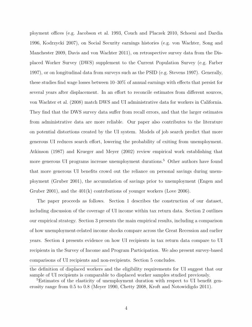
An appealing feature of our data is that, unlike survey data, tax return data provide

highly accurate coverage of UI income. The solid line in Figure 1 plots the annual amount

of all UI payments made, as reported by the Department of Labor. The dotted line with

diamond markers plots the imputed annual amount of UI income reported to the IRS. This

amount is computed by summing over reported UI amounts for the CWHS sample, and then

scaling up to reflect the random sampling of the CWHS.10 Figure 1 depicts the remarkable

quality of tax return data. Between 1999 and 2011, the weighted sum of UI income in all

CWHS tax returns accounts for over 96% of total UI payments. The dotted line with square

9 UI receipt in a single year could represent multiple short spells. SIPP data indicatethat, among households receiving UI income at any point during full calendar years observedin the 2001, 2004, or 2008 panels, 20% experience multiple spells of unemployment.

10We take the maximum amount of UI reported on either the 1040 or the collection of1099-G forms associated with a particular filing unit.

6

markers represents the imputed sum of UI income reported by households that meet all of our

sample restrictions. While each sample restriction lowers the share of UI payments captured

in the analysis sample, restricting to primary filers 60 or younger has the greatest impact.

This age restriction matters the most during the Great Recession. Averaged across all years,

the imputed UI income represented in our analysis sample is 64% of all UI payments made.

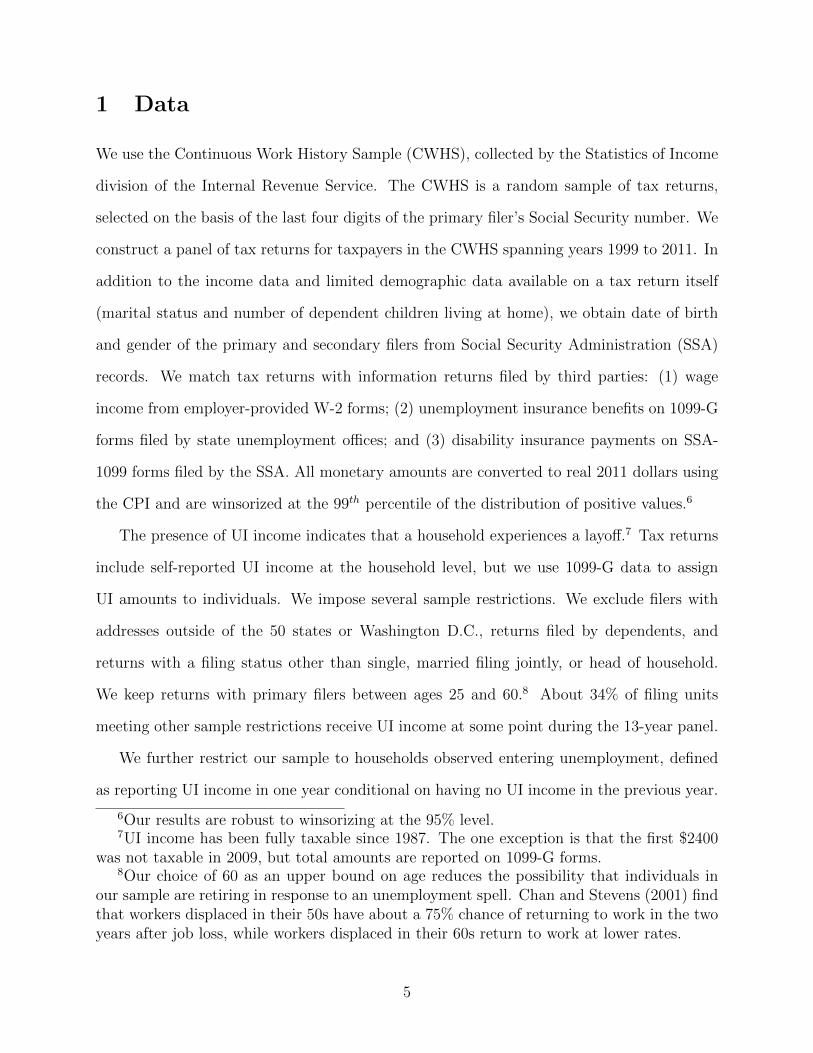
A potential concern is that UI recipients are not representative of the full unemployed

population. We consider this issue in detail in section 4, but here we show that broad

trends in the unemployment rate are replicated in tax data. Figure 2 compares the annual

unemployment rate, as computed by the Bureau of Labor Statistics, to the annual percentage

of primary and secondary filers in the CWHS sample reporting any UI income. The two series

move together, with both increasing during recessions. Their correlation is 0.939. This offers

some assurance that aggregate unemployment trends are represented in tax return data.11

We analyze wage income and various types of non-wage income. Complete variable

definitions are in the Data Appendix, but we provide some description of our income variables

here. Wage income is reported at the household level on a tax return. We construct the

wages of the unemployed individual as the wage income of the person within a household

for whom a 1099-G has been filed.12 We define a composite measure of non-wage income as

total taxable income net of wages and UI benefits. Components of this measure that we also

analyze separately are net capital gains realizations, self-employment income from Schedule

C, and gross distributions from retirement accounts.13 Social Security Disability Insurance

(SSDI) income is not taxable, but is observable from information returns.14

11The ratio of the number of unemployed individuals to the civilian population follows asimilar pattern over time.

12If both the primary and secondary filers receive UI benefits in the same year, we definethe wages of the unemployed individual as the sum of primary and secondary wage income.This occurs in only 1.6% of household-years with UI receipt.

13Individuals in our sample (no older than 60) will in many cases trigger a penalty whentaking distributions from a retirement account. We have examined this penalty amount asan additional dependent variable, finding that it closely tracks retirement distributions.

14Other potentially interesting outcomes not reported on a tax return are net wealth,savings account balances, in-kind or cash transfers in the form of food stamps or welfare, or

7

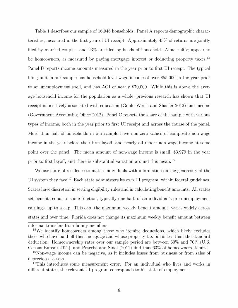
Table 1 describes our sample of 16,946 households. Panel A reports demographic charac-

teristics, measured in the first year of UI receipt. Approximately 43% of returns are jointly

filed by married couples, and 23% are filed by heads of household. Almost 40% appear to

be homeowners, as measured by paying mortgage interest or deducting property taxes.15

Panel B reports income amounts measured in the year prior to first UI receipt. The typical

filing unit in our sample has household-level wage income of over $55,000 in the year prior

to an unemployment spell, and has AGI of nearly $70,000. While this is above the aver-

age household income for the population as a whole, previous research has shown that UI

receipt is positively associated with education (Gould-Werth and Shaefer 2012) and income

(Government Accounting Office 2012). Panel C reports the share of the sample with various

types of income, both in the year prior to first UI receipt and across the course of the panel.

More than half of households in our sample have non-zero values of composite non-wage

income in the year before their first layoff, and nearly all report non-wage income at some

point over the panel. The mean amount of non-wage income is small, $3,979 in the year

prior to first layoff, and there is substantial variation around this mean.16

We use state of residence to match individuals with information on the generosity of the

UI system they face.17 Each state administers its own UI program, within federal guidelines.

States have discretion in setting eligibility rules and in calculating benefit amounts. All states

set benefits equal to some fraction, typically one half, of an individual’s pre-unemployment

earnings, up to a cap. This cap, the maximum weekly benefit amount, varies widely across

states and over time. Florida does not change its maximum weekly benefit amount between

informal transfers from family members.15We identify homeowners among those who itemize deductions, which likely excludes

those who have paid off their mortgage and whose property tax bill is less than the standarddeduction. Homeownership rates over our sample period are between 60% and 70% (U.S.Census Bureau 2012), and Poterba and Sinai (2011) find that 63% of homeowners itemize.

16Non-wage income can be negative, as it includes losses from business or from sales ofdepreciated assets.

17This introduces some measurement error. For an individual who lives and works indifferent states, the relevant UI program corresponds to his state of employment.

8

1999 and 2011, but all other states make a change at some point. Most states change the

maximum benefit amount several times. The mean number of changes is seven, and 19 states

provide a different maximum benefit amount in every year of our analysis. As is standard in

the UI literature, we use the maximum weekly benefit amount at the time of an individual’s

entry into unemployment as a summary measure of the benefit generosity he faces.

Because behavior may differ in short and long spells, it would be useful to know un-

employment spell length. However, we observe only annual UI income. We impute the

number of weeks of UI receipt by dividing annual UI income by a predicted weekly benefit

amount. We have coded the state- and year-specific benefit calculation formulas, as described

in the Department of Labor’s annual Comparison of State Unemployment Insurance Laws.

Each state’s benefit calculation is an increasing function of earnings in a pre-unemployment

base period. We use wage income from the year before UI receipt as our measure of pre-

unemployment earnings and assume that this wage income was spread evenly throughout the

year.18 This procedure, though imperfect, captures business-cycle variation in the average

length of unemployment spells. The average imputed spell length is substantially higher in

2009 through 2011 and is elevated during the recession of the early 2000s.

2 Estimation Strategy

We first consider how wage and salary income changes through unemployment. We estimate

a fixed effects regression model of the following form:

WageIncit = β0 + β1FirstUnempit + β2PostUnempit + β3LaterUnempit

+XitΩ + αi + γt + εit, (1)

18Many state formulas use the highest quarterly earnings in calculating benefits. If wageincome is unevenly spread across the year, we will understate highest quarterly earnings,downward-biasing predicted weekly benefits and upward-biasing imputed weeks of UI receipt.Consistent with this possibility, 9% of primary filers’ UI spells and 16% of secondary filers’UI spells are imputed to involve more than 52 weeks within a calendar year.

9

where i indicates filing unit and t indicates tax year. In some specifications wage and salary

income is measured at the household level, and in other cases it refers to the wage income of

the individual who receives UI. The variable FirstUnemp is an indicator equal to one during

the first unemployment spell and zero otherwise. The variable PostUnemp is a dummy

variable that equals one in all years after the first unemployment spell that the household

does not receive UI. The LaterUnemp term equals one in years with UI receipt after the first

spell of unemployment and zero otherwise. The vector X includes the age and age squared

of the primary filer. The terms αi and γt are filing unit and year fixed effects. Standard

errors are clustered at the tax filing unit level.

Our estimation strategy makes use of variation over time within a filing unit. The coeffi-

cient on FirstUnemp represents the change in income in the first unemployment spell relative

to a filing unit’s average income in pre-unemployment years. We expect that β1 < 0. If wage

income does not recover within our time frame, then β2 would also be negative to reflect a

longer-run reduction in household wage income. Households may experience multiple layoffs

over the course of the panel. The coefficient on LaterUnemp represents the change in wage

income experienced in second and all subsequent unemployment spells relative to the wage

income reported prior to the first observed entry into unemployment. We expect that β3 < 0.

Previous research has shown that the generosity of UI benefits may crowd out job search

efforts of the unemployed, thereby prolonging unemployment spells. Although we do not

observe unemployment duration or search effort in tax return data, we can still estimate

the extent to which more generous benefits alter behavior. Longer unemployment spells will

produce lower values of annual wage income. To measure potential crowd-out, we augment

Equation 1 with three new variables as follows:

WageIncit = β0 + β1FirstUnempit + β2PostUnempit + β3LaterUnempit + β4MaxWBA

+ β5MaxWBA · FirstUnempit + β6MaxWBA · LaterUnempit

+XitΩ + αi + γt + εit, (2)

10

where MaxWBA measures the statutory maximum weekly UI benefit amount an individual

could receive. This term varies with state of residence and year of entry into unemployment,

but not with an individual’s own past wage history.19 Thus, while actual UI benefits depend

on an individual’s pre-unemployment wages, our generosity measure relies only on variation

in benefit generosity that is exogenous to individual characteristics. The interaction terms of

MaxWBA and unemployment spell indicators allow us to estimate the extent to which more

generous UI benefits affect the level of wage income reported during a spell of unemployment.

Negative estimates of β5 and β6 indicate crowd-out; when UI benefits are more generous, wage

income falls more during an unemployment spell than when UI benefits are less generous.

Additionally, we estimate a more flexible specification that accounts for the possibility

that wage income may start to decline prior to the start of unemployment and may recover

only slowly afterwards. Closely following a specification adopted by Jacobson et al. (1993)

and widely used in the subsequent literature, we include a series of dummies measuring the

number of years elapsed since an unemployment spell:

WageIncomeit =9∑

k=−2

(δk ·Dkit) +XitΩ + αi + γt + εit. (3)

In this equation the dummy variables Dk, k = −2, ..., 9, indicate that an observation occurs

k years after a household’s first observed layoff.20 Negative values indicate years prior to first

UI receipt. The D0 dummy is equivalent to the FirstUnemp dummy included in Equation

1. Because households can experience multiple layoffs, positive values, denoting years after

the first spell of UI receipt, may include years with UI receipt. With the smallest value of

k equal to -2, the estimates of δk can be interpreted as the change in wages k years after

entering unemployment, relative to wage income averaged over the observations more than

19Benefit generosity is determined at the start of a spell, and remains constant over thatspell.

20In Jacobson et al. (1993), each time period is a quarter rather than a year. Because wehave annual data, our estimates of wage dynamics around the time of layoff are not directlycomparable to theirs.

11

two years prior to the first layoff.

To investigate whether and to what extent households turn to non-wage income during

an unemployment spell, we use both Equations 1 and 3, changing the dependent variable to

the measures of non-wage income described in Section 1. Although we have estimated both

equations for each type of non-wage income, we present a subset of results. Equation 1 is

appropriate for types of income that can be adjusted very quickly, contemporaneous with

layoff. Equation 3 is most suited to income types that can only be adjusted more slowly.

A state’s UI generosity may influence the utilization of non-wage income sources. To

explore these potential effects, we estimate Equation 2 for non-wage income measures. The

predicted impact of UI generosity on non-wage income is ambiguous. UI benefits may sub-

stitute for other non-wage income sources as a means of smoothing consumption over an

unemployment spell. The larger the share of wage losses that are covered through the UI

system, the less likely a household may be to rely on other income sources. In this case,

more generous UI would crowd out the utilization of non-wage income. Alternatively, if more

generous UI benefits reduce job search effort and lengthen unemployment, households may

be more reliant on non-wage income after job loss. In other words, the crowding out of an

individual’s search effort and wage income by more generous UI benefits could be associated

with the “crowding in” of non-wage income during unemployment spells.

We examine several potential sources of heterogeneity. We split the sample by pre-

unemployment AGI, by household demographic characteristics (age of the primary filer, mar-

ital status, gender, and the presence of children in the household), by imputed spell length,

and by economic conditions that a household faced when it first entered unemployment.

For pre-unemployment AGI and age, we split the sample into those with above-median and

below-median values in the year prior to the first unemployment spell. For spell length, we

split the sample into those with above-median and below-median spell lengths during their

first unemployment spell. Previous research documents that displacements involve much

larger wage losses during a recession than in an expansion (Davis and von Wachter 2011).

12

Therefore we also split the sample into those facing above-median and below-median state

unemployment rates, and we consider whether responses to unemployment were different

before and after the Great Recession began.

3 Results

3.1 Wage Income

Before turning to our regression results, Figure 3 presents graphical evidence on the time

path of wage income in years before and after unemployment. The left panel plots average

annual household-level wage and salary income from eight years before the first UI receipt

to eight years after the first UI receipt. The right panel plots average total income. In these

figures, zero indicates the first year(s) in which a household receives UI income. For spells

that occur over two years, both of these years are included in t = 0. Because households can

enter unemployment spells in different calendar years, characterized by different aggregate

economic conditions, we plot average income net of year fixed effects. Households may

experience multiple unemployment spells, so years included in t > 0 may also be associated

with UI receipt. There are significant wage declines in the year that a household member

becomes unemployed. On average, wage income falls by about $13,000 in that year. Declines

in wage income appear to begin in the year prior to the first receipt of UI. This pattern could

reflect a delay between becoming unemployed and applying for UI, or it could reflect a wage

decline in advance of a future job loss. When a household enters unemployment, total income

falls sharply, with an average decline of over $6,000. The decline in total income is smaller

than the decline in wage income both because UI payments partially compensate for lost

wages, and because non-wage income increases.

Table 2 presents results from fixed-effects regressions describing how wage income changes

during unemployment. The first two columns correspond to Equation 1, with the dependent

variable of annual wage and salary income measured at the household level in column 1

13

and for the unemployed individual in column 2.21 Both columns show a similar pattern. A

first unemployment spell is associated with declines of about $9,300 in annual wage income,

relative to wages in pre-unemployment years. These losses are large; relative to the average

wage income amounts in the year prior to an unemployment spell, these changes represent

a 17% percent decline in annual household wage income and a 23% decline in annual wage

income for the individual who becomes unemployed. Wage income remains significantly

depressed in later years, as shown by the negative coefficient on PostUnemp. On average,

years following an initial unemployment spell are characterized by wage income at least

$8,000 lower than pre-unemployment average annual earnings. Relative to the year prior to

the first unemployment spell, later spells of unemployment are associated with annual wage

losses of over $10,000 at the household level and about $8,700 at the individual level.22

Figure 4 presents the results of estimating Equation 3. The first panel considers annual

household-level wage income, and the second considers annual wages of the unemployed

individual. The coefficients on the D−2 through D9 dummies show the change in annual wage

income relative to wages averaged over observations three or more years prior to entering

unemployment. These results show evidence of substantial declines in wage income in years

of first UI receipt, followed by very slow recovery. It takes six years for household-level

wage income to recover to its pre-unemployment level. Individual-level wage income does

not recover until nine years after unemployment entry. In interpreting these results, it is

important to note that only the first unemployment spell is counted as t = 0. A major reason

that average wage income is low in subsequent years is that some individuals experience

additional unemployment spells.23 The long-run negative wage impacts we document here,

21We also estimate these equations using log annual wages as our dependent variable.For log of household-level wage income, the coefficient on FirstUnemp is -0.35, statisticallysignificant at the 1% level (N = 133,501). We present level specifications of our non-wageregressions because many households do not have certain types of income. Thus we focus onthe level specification when considering wage income to facilitate comparison of estimatedcoefficients across specifications.

22Results are robust to including state fixed effects, as are results in all subsequent tables.23In a previous version of this paper, we analyzed only filing units experiencing a single

14

while substantial, are not as severe as earlier estimates. Jacobson et al. (1993) estimate that

six years after job displacement, earnings losses are 25% of pre-displacement earnings. Couch

and Placzek (2010) estimate earnings losses of 12% to 15% measured six years after mass

layoff. We find that individual-level earnings six years after a first layoff are $2,830 lower

than average pre-unemployment earnings, representing a loss of 7%. It must be noted that

results are not perfectly comparable across studies, as we observe wage income at annual

frequency and previous authors observed quarterly earnings.

Columns 3 and 4 of Table 2 add measures of state UI generosity to investigate the

extent to which UI benefits crowd out wage income. Again, results are similar when wage

income is measured at the household level and at the individual level. Wage income declines

substantially during a first unemployment spell, and it declines by more in cases where

UI benefits are more generous. If UI benefits were zero, a first unemployment spell would

be associated with average wage losses of about $6,600. Each additional hundred dollars

of maximum weekly benefit amount is associated with about $725 less in individual-level

annual wage income during a first unemployment spell ($758 less at the household level).

To put this in context, we compute an elasticity showing the percentage change in annual

wage income associated with a 1% change in the maximum weekly UI benefit. In our

sample, the average wage income of unemployed individuals in the year before a first layoff

is $39,735 and the average maximum weekly benefit amount during a first spell is $368. The

corresponding elasticity of individual wage income with respect to weekly benefit generosity

is −725/39,735100/368

= −0.067. In other words, a 10% increase in benefit generosity is associated

with a 0.67% reduction in annual wage income.

The crowd-out associated with subsequent UI receipt is substantially larger. In these

spells, an additional $100 of maximum weekly UI benefit reduces annual individual-level

wage income by $1,831. Given the average WBA of $381 for later spells, the implied elastic-

ity indicates that a 10% increase in benefit generosity during a second or later spell reduces

spell of UI receipt over the sample period. For that group, wage income had recovered topre-unemployment levels by four to five years after layoff.

15

annual wage income by 1.6%. The greater degree of crowd-out for later spells could be a

result of differences in a behavioral parameter, the elasticity of unemployment duration with

respect to benefit generosity, across those who experience just one unemployment spell and

those with multiple spells. It could also reflect the fact that, by definition, later spells tend

to occur towards the end of the panel. About 55% of second and subsequent unemploy-

ment spells occur during the last four years of our sample. These Great Recession years are

characterized by both high levels of UI benefit generosity and particularly long average un-

employment duration, and Card, Johnston, Leung, Mas and Pei (2015) find a high elasticity

of unemployment duration with respect to benefit generosity during the Great Recession.

There are numerous estimates in the literature of the extent to which greater generosity

of UI benefits increases the duration of unemployment spells. Making some assumptions,

these estimates can be converted to an implied effect on annual wage income, useful for

checking whether our results are of plausible magnitude. Meyer (1990) estimates that a 10%

increase in UI benefit generosity is associated with an 8% increase in unemployment duration.

Individuals in his sample receive UI benefits for an average of 13 weeks, so an 8% increase

in duration corresponds to roughly one additional week of unemployment. This is 1/52, or

1.9%, of the available time in a year. Assuming that wage income is spread evenly over the

year, and that weekly wages are similar pre- and post-unemployment, this suggests that a

10% increase in UI benefit generosity would be associated with a 1.9% reduction in annual

wage income. This is substantially larger than our imputed elasticity for first unemployment

spells, but very close to our elasticity estimate for subsequent spells.

Figure 5 presents evidence on how the size of the wage loss associated with a layoff varies

when wage equations, corresponding to Equation 1, are estimated separately for different

subsamples. The horizontal axis represents the dollar value of wage loss, with more negative

values to the left. Point estimates of the coefficient on FirstUnemp are plotted as circles,

and 95% confidence intervals are plotted as horizontal lines. Not surprisingly, the dollar

value of unemployment-related wage losses is larger for high-AGI filers. Shorter spells are

16

associated with smaller wage losses. The difference between short and long spells persists

when we consider the log of wage income instead of wage levels. Unmarried filers experience

larger wage losses than married filers, both in levels and in logs. Other differences apparent

in Figure 5, particularly the larger wage losses for men than for women and the larger wage

losses for those with some previous receipt of non-wage income, are much less pronounced

when wages are measured in logs. All log income results are available upon request.

3.2 Non-Wage Income

Our results confirm that wage losses associated with unemployment are substantial. The

financial assistance provided by the UI system compensates for only a portion of household

wage losses experienced during unemployment. Average annual UI income is $4,470 during

first unemployment spells and $5,137 during subsequent spells. These values correspond

to 48% of household-level wage losses in first spells and 51% of losses in subsequent spells.

Thus, even with the UI safety net in place, there remain substantial income losses with which

households must cope, either by reducing consumption or by finding income elsewhere.

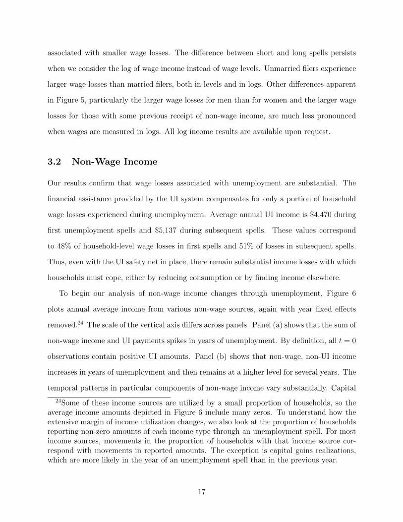
To begin our analysis of non-wage income changes through unemployment, Figure 6

plots annual average income from various non-wage sources, again with year fixed effects

removed.24 The scale of the vertical axis differs across panels. Panel (a) shows that the sum of

non-wage income and UI payments spikes in years of unemployment. By definition, all t = 0

observations contain positive UI amounts. Panel (b) shows that non-wage, non-UI income

increases in years of unemployment and then remains at a higher level for several years. The

temporal patterns in particular components of non-wage income vary substantially. Capital

24Some of these income sources are utilized by a small proportion of households, so theaverage income amounts depicted in Figure 6 include many zeros. To understand how theextensive margin of income utilization changes, we also look at the proportion of householdsreporting non-zero amounts of each income type through an unemployment spell. For mostincome sources, movements in the proportion of households with that income source cor-respond with movements in reported amounts. The exception is capital gains realizations,which are more likely in the year of an unemployment spell than in the previous year.

17

gains realizations display no striking change at the time of unemployment. Distributions

from retirement accounts increase sharply during unemployment and then quickly fall to

slightly above average pre-unemployment levels. In contrast, self-employment income and

disability insurance income show long-run increases. For self-employment income, there is

an immediate but small increase followed by continued growth, while the increase in SSDI

income occurs with a lag after entry into unemployment.

Results showing how several types of non-wage income are adjusted during a spell of

unemployment are shown in Table 3.25 Each column corresponds to a different dependent

variable, using the specification described by Equation 1. The first column considers to-

tal non-wage, non-UI income. This includes specific components considered below (capital

gains, self-employment income, and retirement income) as well as less-frequently observed

types of income such as alimony payments, income from partnerships or S corporations, and

farm income. This composite measure of non-wage income increases by $1,024 in a first

spell of unemployment. Comparing this to the household-level wage loss of $9,331, from

column 1 of Table 2, we see that increased non-wage, non-UI income compensates for about

11% of the wage loss associated with a layoff. Non-wage income remains elevated in the

following years, but does not increase any further during subsequent spells of UI receipt.

This characterizes the average non-wage response, and responses may differ for households

entering unemployment spells expected to be temporary and for households entering what

they expect to be very long spells. We expect that households for whom UI receipt triggers

a permanent decline in income are less likely to smooth consumption by selling assets or

borrowing from retirement accounts, but we are unable to test this hypothesis empirically.

Next, we consider specific components of non-wage income to disentangle which drive

the overall response. Column 2 shows no evidence that capital gains realizations increase

25As we explain later, SSDI income cannot be adjusted as quickly as other types of income.Estimates of Equation 1 using SSDI as a dependent variable confirm this short-run non-responsiveness. Thus, we focus on the dynamic estimation model for SSDI.

18

during or after unemployment.26 One reason that the average response is small is that capital

gains realizations are zero for most of the sample. Only 28% of filing units in our sample

ever report non-zero capital gains. In a regression predicting whether a return includes any

capital gains, we find that receiving UI is associated with a 0.5% increase in the probability

of capital gains realization and this increase is statistically significant at the 5% level. A

second potential reason for the small average effect is that capital gains can be negative

when households sell assets at a loss. If households are simultaneously selling assets that

have appreciated and depreciated, net capital gains realizations will not adequately measure

the resources transferred out of equity portfolios during unemployment. To investigate this

possibility we also estimate regressions in which the dependent variable is net proceeds from

equity sales. We find that net proceeds from equity sales increase during first and subsequent

unemployment spells, but by small amounts not significantly different from zero.

In results not presented, we additionally examine two other sources of investment income:

interest income and dividend income. Interest income is related to the stock of wealth

accumulated in traditional savings accounts, and in principle might proxy for savings account

balances. If individuals respond to a layoff by withdrawing funds from savings accounts,

we would expect to see lower levels of interest income during and after an unemployment

spell. We find virtually no change in interest income during and after unemployment. The

non-responsiveness of interest income likely reflects that interest is an imperfect proxy for

wealth. We also find no evidence that dividend income changes significantly during or after

unemployment. This is likely explained by the limited control an individual has over the

timing of dividend distributions.

Column 3 of Table 3 considers self-employment income, which can encompass a wide range

26The timing of capital gains realizations has been shown to be quite sensitive to taxtreatment (Burman and Randolph 1994). Given that the maximum statutory rate on long-term capital gains fell from 20% to 15% in May 2003, we might expect to see a discretechange in capital gains realizations partway through the panel. The inclusion of year fixedeffects in our regression will account for any effect of this statutory rate change that wasconstant across states.

19

of activities, including starting up a formal business or taking on temporary assignments

as a consultant. The relationship between unemployment and self-employment income is

uncertain, a priori. On one hand, job loss could encourage new participation in the self-

employment sector. On the other hand, periods of high unemployment are also periods of

low aggregate demand, when the probability of small business failure may be particularly

high.27 We find a small negative response in reported self-employment income during years

of unemployment, with a larger positive response in years following a first layoff. Our self-

employment income variable likely measures only a portion of the actual involvement in

self-employment because of under-the-table payments that are not reported to the IRS. An

extensive literature documents higher levels of tax evasion among self-employed individuals

than among those working for employers (Slemrod 2007). Thus, the response we estimate

along the self-employment margin may be thought of as a lower bound on the true self-

employment response.

As foreshadowed by our graphical evidence, by far the largest short-run source of non-

wage income during unemployment is retirement distributions, shown in column 4. On

average, retirement distributions are $4,119 higher during a first unemployment spell than

in years before. In post-unemployment years, retirement distributions continue to be ele-

vated above pre-unemployment levels, by about $550. There is a $1,902 average increase in

retirement distributions during subsequent unemployment spells. We do not observe retire-

ment account balances in our data, but data from the Survey of Consumer Finances provide

a relevant point of comparison. About half of households had retirement accounts in 2010.

Conditional on having a retirement account, the median 2010 balance (expressed in 2011

dollars, for comparability with our estimates) was $45,575 (Federal Reserve Bulletin 2014).

Thus, the average distribution taken during unemployment is not trivial relative to typi-

27Fairlie (2013) analyzes a time period overlapping with our analysis, 1996 to 2009, andfinds a positive relationship between local unemployment rates and entry into entrepreneur-ship, but evidence from earlier time periods and using different data and empirical specifi-cations presents a mixed picture (Evans and Leighton 1989, Parker 2004).

20

cal account balances. Households taking early distributions face an immediate cost in the

form of a penalty owed to the IRS. In our sample, the average penalty paid by a household

taking a retirement distribution in a year with UI income is $545. Households also face a

longer-term cost in the form of lower accumulated savings at the time of retirement. Our

data are not particularly well suited to estimating this longer-term cost. A study of a much

broader range of factors contributing to retirement account “leakage,” of which penalized

early withdrawals are one type, finds that aggregate 401(k) and IRA wealth is about 20%

lower than it would be in the absence of any leakage at all (Munnell and Webb 2015).

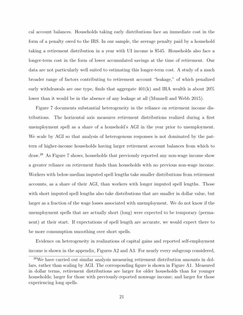
Figure 7 documents substantial heterogeneity in the reliance on retirement income dis-

tributions. The horizontal axis measures retirement distributions realized during a first

unemployment spell as a share of a household’s AGI in the year prior to unemployment.

We scale by AGI so that analysis of heterogenous responses is not dominated by the pat-

tern of higher-income households having larger retirement account balances from which to

draw.28 As Figure 7 shows, households that previously reported any non-wage income show

a greater reliance on retirement funds than households with no previous non-wage income.

Workers with below-median imputed spell lengths take smaller distributions from retirement

accounts, as a share of their AGI, than workers with longer imputed spell lengths. Those

with short imputed spell lengths also take distributions that are smaller in dollar value, but

larger as a fraction of the wage losses associated with unemployment. We do not know if the

unemployment spells that are actually short (long) were expected to be temporary (perma-

nent) at their start. If expectations of spell length are accurate, we would expect there to

be more consumption smoothing over short spells.

Evidence on heterogeneity in realizations of capital gains and reported self-employment

income is shown in the appendix, Figures A2 and A3. For nearly every subgroup considered,

28We have carried out similar analysis measuring retirement distribution amounts in dol-lars, rather than scaling by AGI. The corresponding figure is shown in Figure A1. Measuredin dollar terms, retirement distributions are larger for older households than for youngerhouseholds; larger for those with previously-reported nonwage income; and larger for thoseexperiencing long spells.

21

capital gains realizations are not statistically different from zero. Comparing those with

short imputed spell length to those with long imputed spell length, there is no significant

difference in realizations of capital gains. Considering self-employment income, the most

noteworthy difference across groups appears when we split the sample on the presence of

any non-wage income prior to unemployment. Those with no previous non-wage income

report significantly more self-employment income during a first unemployment spell. There

is very little difference in the self-employment income response of those with short and long

spells. This may reflect the fact that when a person enters into a spell of unemployment, she

does not know if it is going to be temporary or permanent, and so it may be difficult to know

whether incurring the start-up costs of entering into self-employment will be worthwhile.

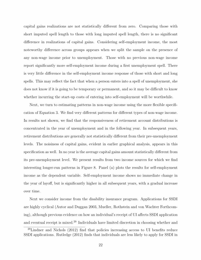
Next, we turn to estimating patterns in non-wage income using the more flexible specifi-

cation of Equation 3. We find very different patterns for different types of non-wage income.

In results not shown, we find that the responsiveness of retirement account distributions is

concentrated in the year of unemployment and in the following year. In subsequent years,

retirement distributions are generally not statistically different from their pre-unemployment

levels. The noisiness of capital gains, evident in earlier graphical analysis, appears in this

specification as well. In no year is the average capital gains amount statistically different from

its pre-unemployment level. We present results from two income sources for which we find

interesting longer-run patterns in Figure 8. Panel (a) plots the results for self-employment

income as the dependent variable. Self-employment income shows no immediate change in

the year of layoff, but is significantly higher in all subsequent years, with a gradual increase

over time.

Next we consider income from the disability insurance program. Applications for SSDI

are highly cyclical (Autor and Duggan 2003, Mueller, Rothstein and von Wachter Forthcom-

ing), although previous evidence on how an individual’s receipt of UI affects SSDI application

and eventual receipt is mixed.29 Individuals have limited discretion in choosing whether and

29Lindner and Nichols (2012) find that policies increasing access to UI benefits reduceSSDI applications. Rutledge (2012) finds that individuals are less likely to apply for SSDI in

22

when to receive SSDI income. Even if the initial decision to apply for benefits is responsive

to unemployment, applications go through a five-step review process that includes review by

medical examiners. Only about 26% of applications are approved when first considered. Re-

jected applicants can appeal, and approximately 41% of applications are ultimately approved

(Social Security Administration 2013). This process makes it likely that any relationship be-

tween job displacement and SSDI receipt occurs with a lag. Panel (b) of Figure 8 documents

how SSDI income evolves over time in our sample. There is no change in SSDI income con-

current with the first receipt of UI income. In every subsequent year, average SSDI income is

significantly above its pre-unemployment average level, and SSDI income continues to grow

over time. This pattern is driven by changes in receipt of any SSDI, rather than changes

in the amount of SSDI conditional on receipt. The percentage of our sample receiving any

SSDI is less than 1% in years prior to unemployment, before eventually growing to approxi-

mately 4%. Our results can be reconciled with the findings of Mueller et al. (Forthcoming).

Using aggregate data, they find essentially no contemporaneous relationship between rates

of UI exhaustion and rates of SSDI application, nor do they find evidence of increased SSDI

applications up to three months after UI exhaustion. Using administrative-level data, they

find little or no effect of UI extensions on SSDI applications up to four weeks following a UI

extension. Our ability to consider longer-run responses is an important advantage of using

tax return data to measure SSDI receipt.

Table 4 provides estimates of Equation 2 for non-wage income, investigating how UI

generosity affects reliance on non-wage income. We find no evidence that UI generosity

impacts total non-wage, non-UI income or net capital gains realizations. In the case of self-

employment income, raising the maximum weekly UI benefit amount by $100 is associated

with a $187 smaller change in Schedule C income during a first layoff. The strongest evi-

dence of an interaction between UI benefit generosity and non-wage income is in the case of

months when UI benefits are extended, and are more likely to apply in months when benefitsare exhausted. In contrast, Mueller et al. (Forthcoming) find no evidence that UI benefitexhaustion is associated with an increased rate of SSDI application.

23

retirement distributions. The UI generosity interaction terms are positive, indicating that

households facing more generous UI benefits take greater distributions from their retirement

accounts during an unemployment spell. Although this is a surprising result, it might be

explained by changes in job search behavior with respect to UI generosity. Previous research

has shown that more generous UI benefits are associated with longer unemployment dura-

tions. Longer unemployment spells may be precisely the situations that prompt individuals

to take distributions from retirement accounts. Indeed, Figure 7 shows this to be the case.

Comparing the dollar amounts of additional wage loss and additional retirement distribu-

tions associated with more generous UI benefits shows similar orders of magnitude. For a

first unemployment spell, an additional $100 of weekly maximum UI benefit amount is as-

sociated with a further $758 decline in household-level annual wage income (see column 3 of

Table 2) and an additional $1008 of retirement distributions. These amounts are not entirely

dissimilar, and could result from households using withdrawals from retirement accounts to

perfectly smooth consumption during an unemployment spell. This pattern would be consis-

tent with evidence from Browning and Crossley (2001) that households with financial assets

have almost no change in consumption at the time of job loss.30 For subsequent spells, the

additional annual wage loss associated with an extra $100 of maximum weekly benefits is

larger ($1831) than the associated additional retirement distribution ($707). A retirement

account that has already been tapped during a first unemployment spell would plausibly

provide less consumption smoothing during subsequent spells.

3.3 The Great Recession

Our panel provides an opportunity to examine whether and to what extent the Great Re-

cession, which spanned December 2007 through June 2009, changed household experiences

30In additional analysis, we have investigated whether the overall positive relationshipbetween UI benefit generosity and retirement distributions varies across age groups. We finda positive relationship for both younger and older households, with a larger magnitude forolder households. The coefficients and standard errors on the MaxWBA · First Unemp termare $405 (150) for the younger group and $1498 (406) for the older group.

24

during unemployment. To begin, we investigate whether there are differences in the charac-

teristics of individuals experiencing unemployment at different points in time. Table 5 shows

that those receiving UI in 2008 or later are less likely to be married, more likely to be single

men, have fewer children, and are slightly older.31 Perhaps due to the increase in home-

ownership rates through the housing market boom, those who are unemployed in the later

period are more likely to be homeowners. There are statistically significant differences in

household incomes, with those unemployed in 2008 or later having lower pre-unemployment

AGI, but this largely reflects differences in marital status. Controlling for marital status, the

difference between earlier and later household AGI drops by 15% but remains statistically

significant.

To understand how the wage losses from unemployment have varied over time, we esti-

mate the following equation:

WageIncomeit = α +2011∑

j=2000

βjUnempit × (UnempY ear = j) +XitΩ + αi + γt + εit. (4)

In this specification, the indicator variables (UnempY ear = j) equal one if the household

receives UI benefits in year j and zero otherwise. The coefficients, βj, thus capture the

income changes in an unemployment spell in year j relative to income in other years. These

coefficients combine income changes that occur in first unemployment spells and later un-

employment spells.

Figure 9 plots the wage income loss for unemployment spells in 2000 through 2011. The

severity of wage loss appears to vary with the business cycle. Those experiencing unemploy-

ment during the economic boom of 2000 have particularly small wage losses associated with

unemployment. Those who are unemployed between 2009 and 2011 have significantly larger

wage losses than those who are unemployed in pre-Great Recession years.

31We exclude 2007 from this comparison because it contains months before and after thestart of the Great Recession. The summary statistics are very similar when we include 2007as a Recession year.

25

We next examine whether the utilization of non-wage income sources changed through

the Great Recession, estimating versions of Equation 4 with non-wage income amounts

as dependent variables. Although one might expect that unemployment spells involving

the largest wage losses would involve the greatest reliance on non-wage income, we find a

somewhat different pattern. Most income sources display no economically or statistically

different response before and after the Great Recession. In Figure 10, we plot two non-wage

income measures of particular interest given the average responses documented above. The

first panel plots the increase in all non-wage, non-UI income associated with unemployment

spells that occur in each year. There is not a particularly strong reliance on non-wage income

in Great Recession years. Most estimates are not significantly different from zero, which is

not surprising because these estimates pool together first and later spells, and Table 3 showed

little change in aggregate non-wage income during later spells.32 The second panel of Figure

10 shows that, regardless of when an unemployment spell occurs, the reliance on retirement

distributions is substantial. This behavior looks quite similar during Great Recession years

and in earlier years.

The combination of larger wage losses with no discernable increase in the realization of

non-wage income during the Great Recession may be reconciled by an increased reliance on

the social safety net. Bitler and Hoynes (2013) document that major safety net programs

did not provide more protection to the most disadvantaged during the Great Recession, but

those elements of the safety net of greatest importance to higher-income individuals, like

the tax filers in our sample, did provide more protection. The maximum duration of UI

benefit receipt rose to 99 weeks (Rothstein 2011), and recent evidence suggests that the

length of unemployment spells became more sensitive to UI benefit generosity during the

Great Recession (Card et al. 2015). In our data set, we find that annual UI income is

almost exactly 50% of annual wage losses associated with unemployment, both before and

32If we restrict attention to first unemployment spells only, again we find that unemploy-ment spells occurring in the Great Recession years do not involve particularly large relianceon non-wage income.

26

during the Great Recession. In addition, the number of people receiving SNAP benefits

rose from 9% of the population on the eve of the Great Recession to 15% in July 2011, and

most of this increase can be explained by changes in local unemployment rates (Ganong and

Liebman 2013). Either the increase in safety net programs such as UI and SNAP mitigated

the need for individuals to turn to private options, individuals simply did not have the

capacity to increase reliance on assets such as retirement accounts, or consumption fell by

more during unemployment in this more recent period.

4 Selection Into UI Receipt

Our analysis examines households that receive UI benefits, a subset of all unemployed indi-

viduals. Some unemployed individuals are ineligible for UI, either because pre-unemployment

earnings or hours of work fall below eligibility thresholds or because they voluntarily quit

or were fired. Among those who are eligible for UI, not all choose to take up benefits.33

Ebenstein and Stange (2010) calculate UI receipt rates for 1989 to 2006, and find that 47%

of all unemployed individuals are eligible for UI and that 36% receive UI, implying a take-

up rate of 79%. Particularly relevant for our analysis is evidence that the decision to take

up UI benefits is positively correlated with education and with pre-unemployment earnings

(Government Accounting Office 2006, Shaefer 2010). If UI-recipient households have higher

permanent income than unemployed households not receiving UI, then the potential to turn

to non-wage income sources will be higher within our sample than for the population. Sim-

ilarly, if UI recipients have longer unemployment spells involving greater-than-average wage

losses, then we would expect our estimated reliance on non-wage income to be an upper

bound on estimates for a broader sample of unemployed individuals.

We compare unemployed UI recipients and non-recipients using data from the 2001, 2004,

and 2008 panels of the Survey of Income and Program Participation (SIPP). Conducted by

33Important work explaining the factors associated with UI take-up includes Blank andCard (1991) and Anderson and Meyer (1997).

27

the U.S. Census Bureau, the SIPP is a longitudinal survey gathering detailed information

on various sources of earned and transfer income. Each SIPP panel follows individuals

for up to three or four years, with interviews every four months. Information on weekly

employment status is collected, allowing very precise measurement of transitions into and

out of unemployment. Individuals also report income received from UI benefits. We identify

all spells of unemployment experienced by SIPP respondents, and compare spells with and

without receipt of UI income.

We define the start of an unemployment spell as a transition from an employment status of

either working for pay or being temporarily absent from a job without pay, to an employment

status of being on temporary layoff, having no job and looking for work, or having no job

and not looking for work. We define the end of an unemployment spell as four consecutive

weeks of work. We drop spells in which a person’s employment status was always without

a job and not looking for work, as this behavior is considered being out of the labor force

rather than being unemployed. The exception is that we keep a spell if it involved receipt

of UI benefits, even if this person never reported looking for work.34 We restrict attention

to individuals between the ages of 25 and 60.

Summary statistics for the set of unemployment spells meeting these criteria are shown in

columns 1 through 3 of Table 6. Column 1 includes unemployment spells that do not involve

UI receipt. Column 2 focuses on the subset of spells in column 1 that appear eligible for UI

benefits despite not involving benefit receipt.35 Column 3 includes spells in which UI income

is received. Comparing the number of observations in columns 1 and 3, approximately 30% of

spells involve receipt of UI benefits. Spells involving UI receipt are longer, with a mean length

34There are relatively few such spells, 6.4% of all spells involving UI receipt.35Eligibility depends on pre-unemployment earnings and the reason for job separation.

Information on the reason for job separation is unavailable for many unemployment spellsin the SIPP. It is not collected when the reporting of a job separation occurs at the verybeginning of a new reference period (that is, “on the seam” between SIPP interviews). Inthe SIPP, changes in employment status are heavily concentrated on the seam. If there is noinformation available on the reason for job separation, we do not classify an unemploymentspell as UI-eligible.

28

of almost 30 weeks, relative to a mean length of 19.6 weeks for spells without UI receipt. The

mean imputed unemployment spell length in our tax sample, reported in column 4, shows

that the spells identified in tax data are similar in length to spells reported by UI recipients

in the SIPP. We hypothesize that longer spells are more likely to exhaust liquid assets and to

necessitate turning towards assets such as retirement accounts. Compared to non-recipients,

UI recipients are older, more likely to be married, and more likely to be homeowners.

Panel B compares annual income amounts from the SIPP and from tax return data

(shown in column 4 of Table 6, repeated from Table 1). It offers some reassurance about the

reliability of our main estimates, while highlighting the importance of using multiple data

sources to understand responses to unemployment. In tax return data, these amounts are

measured in the calendar year before the year in which UI income is first received. In the

SIPP, annual amounts were computed by aggregating over the 12 months prior to unemploy-

ment entry.36 UI recipients in the SIPP have higher levels of earnings than non-recipients

of UI. Pre-unemployment wage and salary amounts, measured either for the unemployed

individual or for the family including that individual, are similar for UI recipients in the

SIPP and for UI recipients in tax data. The average amount of family-level business in-

come is higher in the SIPP than in tax return data, and the annual amount of distributed

income from retirement accounts is substantially higher in tax return data. Both patterns

are plausible based on what is known about the under-reporting of self-employment income

to tax authorities and the potential to forget infrequently realized income when responding

to a survey. Panel C shows the share of families reporting any income of a particular type,

again measured in the 12 months (SIPP) or calendar year (tax data) prior to unemployment

entry. Values for wage and business income are fairly similar for UI recipients in tax return

data and UI recipients in the SIPP, and are also similar for UI recipients and non-recipients

in the SIPP. There is a difference in the reported receipt of retirement distributions, with

13% of observations in the tax data including retirement distribution income and only 4%

36With fewer than 12 months of earnings data, we scaled up to annual amounts.

29

of SIPP observations reporting retirement distribution income.

The amount of wage income lost during an unemployment spell is likely an important

determinant of reliance on non-wage income. Figure 11 plots average monthly earned income

around the time of entry into unemployment, with panel A showing individual-level earnings

and panel B showing earnings at the household level. The scale on the vertical axis differs

across panels. The drop in monthly earnings is greater for UI recipients than for non-

recipients. The recovery over the following months is slightly greater in absolute terms for

UI recipients, but eleven months after entering unemployment the UI recipients are earning

a lower fraction of their pre-unemployment monthly earnings than the non-recipients are.

We interpret this pattern as additional evidence that the unemployment spells we identify

in tax return data are likely associated with greater reliance on non-wage income than the

unemployment spells we fail to detect.

This analysis is useful for putting our tax-based estimates into context with respect to

the experiences of all households that suffer a job loss. If we are concerned about job losers

with significant labor market attachment, then it appears we are able to identify a large and

representative sample of such spells in tax return data. The observable differences between

UI recipients and those who do not take up UI generally suggest that our estimates represent

an upper bound on the extent to which the full population of unemployed households rely

on non-wage income during unemployment.

5 Conclusions

Unemployment imposes large financial costs on households. By providing comprehensive

measures of income from wages and from non-wage sources, tax return data can offer new

insights into how households cope with the strain of unemployment. Using a panel of tax

return data spanning 1999 to 2011, this paper first estimates the wage losses associated with

unemployment. We find that unemployment is associated with annual wage income declines

30

of about 17% when measured at the household level and about 23% when measured at the

individual level. Wages remain depressed for some time, returning to pre-unemployment lev-

els only after several years. The wage losses associated with a first unemployment spell were

particularly large in 2009-2011, reflecting continued weakness in the labor market following

the Great Recession.

We provide new evidence on the utilization of non-wage income sources by households

through unemployment. The UI system, on average, buffers recipient households from

roughly half of the wage income losses associated with a job loss. Other non-wage, non-

UI income sources compensate for an additional 11% of the wage losses experienced in a

first unemployment spell, but provide much less of a buffer in later unemployment spells.

Tapping into retirement savings is by far the most prevalent short-run response to unemploy-

ment, despite the penalties incurred by taking early distributions from retirement accounts.

This finding suggests that traditional savings balances are insufficient for coping with the

negative income shocks associated with layoffs. We also find evidence of longer-run increases

in income from self-employment and from SSDI after unemployment.

One concern about the UI program is that more generous benefits reduce job search effort.

Consistent with the large literature showing that more generous UI benefits are associated

with longer unemployment spells, we find that more generous benefits are associated with

lower annual wage income. We find smaller crowd-out of wage income in first observed

unemployment spells than in later spells. Overall, we find little evidence that the generosity

of the UI system influences the extent to which households utilize other income sources. The

exception is that more generous UI is associated with an increased reliance on retirement

savings. Coupled with the crowd out of job search effort, this result indicates that a more

generous UI system may lead households to rely even more heavily on savings that have been

set aside for retirement. This interaction should be of concern for policy-makers evaluating

the recent increases in UI generosity, if such expansions of the UI system result in recipients

finding themselves less financially prepared for retirement in the future.

31

References

Addison, John T. and McKinley L. Blackburn, “The Effects of Unemployment Insur-ance on Postunemployment Earnings,” Labour Economics, 2000, 7 (1), 21–53.

Amromin, Gene and Paul Smith, “What Explains Early Withdrawals from RetirementAccounts? Evidence from a Panel of Taxpayers,” National Tax Journal, 2003, 56 (3),595–612.

Anderson, Patricia and Bruce Meyer, “Unemployment Insurance Take-Up Rates andthe After-Tax Value of Benefits,” Quarterly Journal of Economics, 1997, 112, 913–937.

Atkinson, A. B., “Income Maintenance and Social Insurance,” in Alan J. Auerbach andMartin Feldstein, eds., Handbook of Public Economics, Elsevier, 1987, pp. 780–908.

Autor, David H. and Mark G. Duggan, “The Rise in the Disability Rolls and theDecline in Unemployment,” Quarterly Journal of Economics, 2003, 118 (1), 157—206.

Bentolila, Samuel and Andrea Ichino, “Unemployment and Consumption Near andFar Away from the Mediterranean,” Journal of Population Economics, 2008, 21 (2),255–280.

Bitler, Marianne and Hilary Hoynes, “The More Things Change, the More They Staythe Same? The Safety Net and Poverty in the Great Recession,” NBER Working Paper19449 2013.

Blank, Rebecca M. and David E. Card, “Recent Trends in Insured and UninsuredUnemployment: Is There an Explanation?,” Quarterly Journal of Economics, 1991,106 (4), 1157–1189.

Bollinger, Christopher R. and Barry T. Hirsch, “Match Bias from Earnings Imputa-tion in the Current Population Survey: The Case of Imperfect Matching,” Journal ofLabor Economics, 2006, 24 (3), 489–506.

Browning, Martin and Thomas F. Crossley, “Unemployment Insurance Benefit Levelsand Consumption Changes,” Journal of Public Economics, 2001, 80 (1), 1–23.

Burman, Leonard E. and William C. Randolph, “Measuring Permanent Responses toCapital-Gains Tax Changes in Panel Data,” American Economic Review, 1994, 84 (4),794—809.

Card, David, Andrew Johnston, Pauline Leung, Alexandre Mas, and Zhuan Pei,“The Effect of Unemployment Benefits on the Duration of Unemployment InsuranceReceipt: New Evidence from a Regression Kink Design in Missouri, 2003-2013,” NBERWorking Paper 20869 2015.

Chan, Sewin and Ann Huff Stevens, “Job Loss and Employment Patterns of OlderWorkers,” Journal of Labor Economics, 2001, 19 (2), 484–521.

32

Chetty, Raj, “Moral Hazard versus Liquidity and Optimal Unemployment Insurance,”Journal of Political Economy, 2008, 116 (2), 173–234.

Couch, Kenneth A. and Dana W. Placzek, “Earnings Losses of Displaced WorkersRevisited,” American Economic Review, 2010, 100 (1), 572–589.

Davis, Steven J. and Till von Wachter, “Recessions and the Costs of Job Loss,” Brook-ings Papers on Economic Activity, 2011, 43 (2), 1–72.

Dynarski, Susan and Jonathan Gruber, “Can Families Smooth Variable Earnings?,”Brookings Papers on Economic Activity, 1997, 1, 229–303.

Ebenstein, Avraham and Kevin Stange, “Does Inconvenience Explain Low Take-Up?Evidence from Unemployment Insurance,” Journal of Policy Analysis and Management,2010, 29 (1), 111–136.

Engen, Eric M. and Jonathan Gruber, “Unemployment Insurance and PrecautionarySaving,” Journal of Monetary Economics, 2001, 47 (3), 545–579.

Evans, David S. and Linda S. Leighton, “Some Empirical Aspects of Entrepreneurship,”American Economic Revies, 1989, 79 (3), 519–535.

Fairlie, Robert W., “Entrepreneurship, Economic Conditions, and the Great Recession,”Journal of Economics and Management Strategy, 2013, 22 (2), 207–231.

Farber, Henry S., “The Changing Face of Job Loss in the United States, 1981-1995,”Brookings Papers on Economic Activity, Microeconomics, 1997, 1997, 55–128.

Federal Reserve Bulletin, “Changes in U.S. Family Finances from 2010 to 2013: Evidencefrom the Survey of Consumer Finances,” Technical Report 2014.

Ganong, Peter and Jeffrey B. Liebman, “The Decline, Rebound, and Further Rise inSNAP Enrollment: Disentangling Business Cycle Fluctuations and Policy Changes,”NBER Working Paper 19363 2013.

Gould-Werth, Alix and H. Luke Shaefer, “Unemployment Insurance Participation byEducation and by Race and Ethnicity,” Monthly Labor Review, 2012, 135 (10), 28–41.

Government Accounting Office, “Unemployment Insurance: Factors Associated WithBenefit Receipt,” GAO-06-341 2006.

, “Economic Cicumstances of Individuals Who Exhausted Benefits,” GAO-12-408 2012.

Gruber, Jonathan, “The Wealth of the Unemployed,” Industrial and Labor RelationsReview, 2001, 55 (1), 79–94.

Hilger, Nathaniel, “Parental Job Loss and Children’s Long-Term Outcomes: Evidencefrom 7 Million Fathers’ Layoffs,” 2014.

33

Hurst, Erik and Frank Stafford, “Home is Where the Equity Is: Mortgage Refinancingand Household Consumption,” Journal of Money, Credit, and Banking, 2004, 36 (6),985–1014.

Jacobson, Louis S., Robert J. LaLonde, and Daniel G. Sullivan, “Earnings Lossesof Displaced Workers,” American Economic Review, 1993, 83 (4), 685–709.

Kawano, Laura and Sara LaLumia, “The Added Worker Effect: Differential Responsesby Husbands and Wives,” 2014.

Kletzer, Lori G., “Job Displacement,” Journal of Economic Perspectives, 1998, 12 (1),115–136.

Kodrzycki, Yolanda K., “Using Unexpected Recalls to Examine the Long-Term EarningsEffects of Job Displacement,” Federal Reserve Bank of Boston Working Paper 2007.

Kroft, Kory and Matthew J. Notowidigdo, “Should Unemployment Insurance Varywith the Unemployment Rate? Theory and Evidence,” Working Paper 2011.

Krueger, Alan B. and Bruce D. Meyer, “Labor Supply Effects of Social Insurance,” inAlan J. Auerbach and Martin Feldstein, eds., Handbook of Public Economics, Elsevier,2002, pp. 2327–2392.

Lillard, Lee, James P. Smith, and Finis Welch, “What Do We Really Know aboutWages? The Importance of Nonreporting and Census Imputation,” Journal of PoliticalEconomy, 1986, 94 (3, part 1), 489–506.

Lindner, Stephan and Austin Nichols, “The Impact of Temporary Assistance Programson Disability Rolls and Re-Employment,” Working Paper 2012.

Love, David, “Buffer Stock Saving in Retirement Accounts,” Journal of Monetary Eco-nomics, 2006, 53 (7), 1473–1492.

Mathiowetz, Nancy A. and Greg J. Duncan, “Out of Work, Out of Mind: ResponseErrors in Retrospective Reports of Unemployment,” Journal of Business and EconomicStatistics, 1988, 6 (2), 221–229.

Meyer, Bruce D., “Unemployment Insurance and Unemployment Spells,” Econometrica,1990, 58 (4), 757–782.

, Wallace K. C. Mok, and James X Sullivan, “The Under-Reporting of Transfersin Household Surveys: Its Nature and Consequences,” NBER Working Paper 151812009.

Mueller, Andreas I., Jesse Rothstein, and Till M. von Wachter, “Unemployment In-surance and Disability Insurance in the Great Recession,” Journal of Labor Economics,Forthcoming.

Munnell, Alicia H. and Anthony Webb, “The Impact of Leakages from 401(k)s andIRAs,” Center for Retirement Research Working Paper 2015-2 2015.

34

Oyer, Paul, “Recall Bias Among Displaced Workers,” Economics Letters, 2004, 82 (3),397–402.

Parker, Simon C., The Economics of Self-Employment and Entrepreneurship 2004.

Poterba, James and Todd Sinai, “Revenue Costs and Incentive Effects of the MortgageInterest Deduction for Owner-Occupied Housing,” National Tax Journal, 2011, 64 (2),531–564.

Rothstein, Jesse, “Unemployment Insurance and Job Search in the Great Recession,”Brookings Papers on Economic Activity, 2011, Fall, 143–196.

Rutledge, Matthew, “The Impact of Unemployment Insurance Extensions on DisabilityInsurance Application and Allowance Rates,” Working Paper No. 2011-17, Center forRetirement Research at Boston College 2012.

Schoeni, Robert, “Does Unemployment Insurance Displace Familial Assistance?,” PublicChoice, 2002, 110 (1-2), 99–119.

Schoeni, Robert F. and Michael Dardia, “Wage Losses of Displaced Workers in the1990s,” RAND Working Paper 1996.

Shaefer, H. Luke, “Identifying Key Barriers to Unemployment Insurance for Disadvan-taged Workers in the United States,” Journal of Social Policy, 2010, 39 (3), 439–460.

Slemrod, Joel, “Cheating Ourselves: The Economics of Tax Evasion,” Journal of EconomicPerspectives, 2007, 21 (1), 25–48.

Social Security Administration, “Annual Statistical Report on the Social Security Dis-ability Insurance Program, 2012,” Technical Report 2013.

Stephens, Melvin Jr., “The Long-Run Consumption Effects of Earnings Shocks,” Reviewof Economics and Statistics, 2001, 83 (1), 28–36.

Stevens, Ann Huff, “Persistent Effects of Job Displacement: The Importance of MultipleJob Losses,” Journal of Labor Economics, 1997, 15 (1, part 1), 165–188.

Sullivan, James X., “Borrowing During Unemployment: Unsecured Debt as a Safety Net,”Journal of Human Resources, 2008, 43 (2), 383–412.

U.S. Census Bureau, “Statistical Abstract of the United States: 2012,” Technical Report2012.

von Wachter, Till, Jae Song, and Joyce Manchester, “Long-Term Earnings Lossesdue to Mass Layoffs During the 1982 Recession: An Analysis Using U.S. AdministrativeData from 1974 to 2004,” Working Paper 2009.

von Wachter, Till M., Elizabeth Weber Handwerker, and Andrew K. G. Hildreth,“Estimating the ‘True’ Cost of Job Loss: Evidence using Matched Data from California1991-2000,” Working Paper 2008.

35

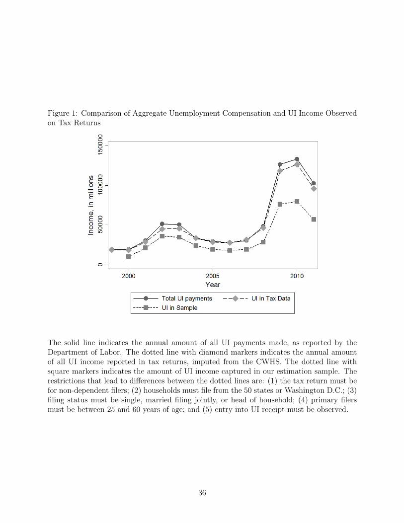
Figure 1: Comparison of Aggregate Unemployment Compensation and UI Income Observedon Tax Returns

The solid line indicates the annual amount of all UI payments made, as reported by theDepartment of Labor. The dotted line with diamond markers indicates the annual amountof all UI income reported in tax returns, imputed from the CWHS. The dotted line withsquare markers indicates the amount of UI income captured in our estimation sample. Therestrictions that lead to differences between the dotted lines are: (1) the tax return must befor non-dependent filers; (2) households must file from the 50 states or Washington D.C.; (3)filing status must be single, married filing jointly, or head of household; (4) primary filersmust be between 25 and 60 years of age; and (5) entry into UI receipt must be observed.

36

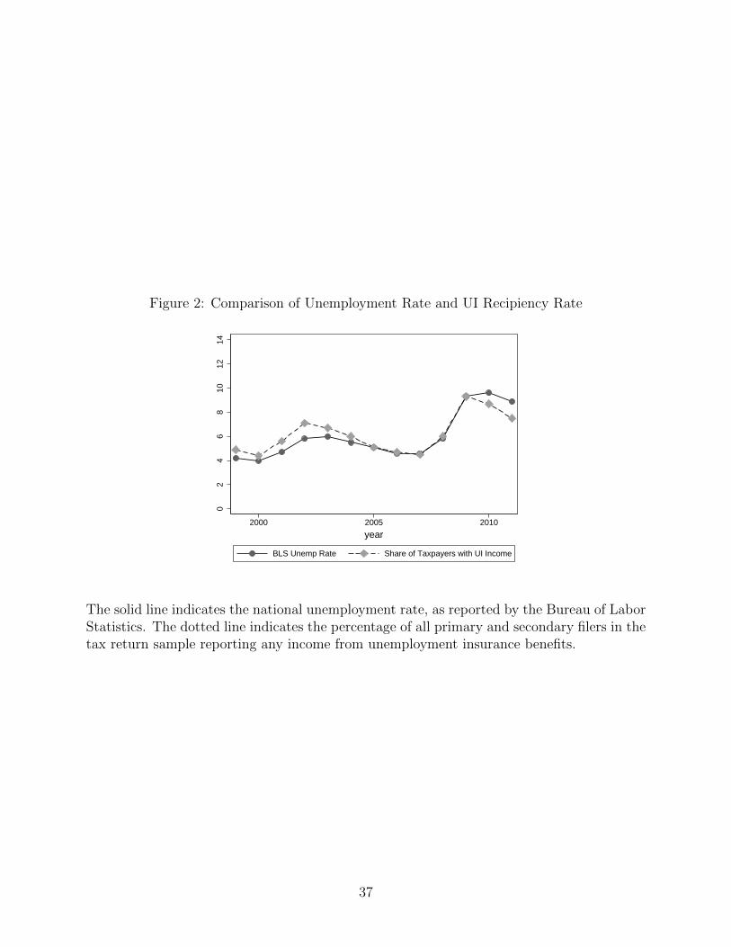
Figure 2: Comparison of Unemployment Rate and UI Recipiency Rate

02

46

810

1214

2000 2005 2010

year

BLS Unemp Rate Share of Taxpayers with UI Income

The solid line indicates the national unemployment rate, as reported by the Bureau of LaborStatistics. The dotted line indicates the percentage of all primary and secondary filers in thetax return sample reporting any income from unemployment insurance benefits.

37

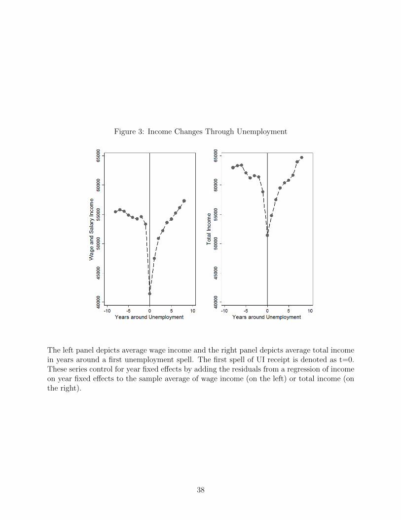
Figure 3: Income Changes Through Unemployment

The left panel depicts average wage income and the right panel depicts average total incomein years around a first unemployment spell. The first spell of UI receipt is denoted as t=0.These series control for year fixed effects by adding the residuals from a regression of incomeon year fixed effects to the sample average of wage income (on the left) or total income (onthe right).

38

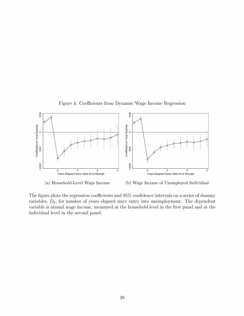
Figure 4: Coefficients from Dynamic Wage Income Regression

−10

000

−50

000

5000

Coe

ffici

ent o

n Y

ear

Dum

my

0 3 6 9

Years Elapsed Since Start of UI Receipt

(a) Household-Level Wage Income

−10

000

−50

000

5000

Coe

ffici

ent o

n Y

ear

Dum

my

0 3 6 9

Years Elapsed Since Start of UI Receipt

(b) Wage Income of Unemployed Individual

The figure plots the regression coefficients and 95% confidence intervals on a series of dummyvariables, Dk, for number of years elapsed since entry into unemployment. The dependentvariable is annual wage income, measured at the household level in the first panel and at theindividual level in the second panel.

39

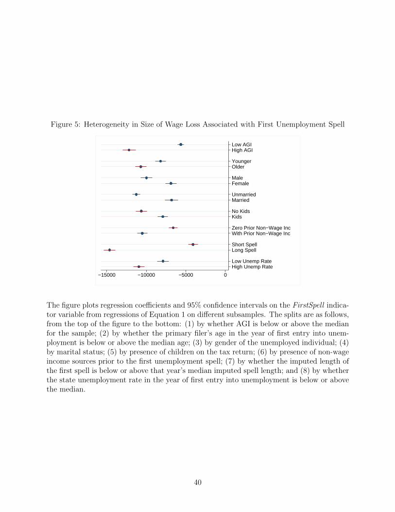
Figure 5: Heterogeneity in Size of Wage Loss Associated with First Unemployment Spell

Low AGIHigh AGI

YoungerOlder

MaleFemale

UnmarriedMarried

No KidsKids

Zero Prior Non−Wage IncWith Prior Non−Wage Inc

Short SpellLong Spell

Low Unemp RateHigh Unemp Rate

−15000 −10000 −5000 0

The figure plots regression coefficients and 95% confidence intervals on the FirstSpell indica-tor variable from regressions of Equation 1 on different subsamples. The splits are as follows,from the top of the figure to the bottom: (1) by whether AGI is below or above the medianfor the sample; (2) by whether the primary filer’s age in the year of first entry into unem-ployment is below or above the median age; (3) by gender of the unemployed individual; (4)by marital status; (5) by presence of children on the tax return; (6) by presence of non-wageincome sources prior to the first unemployment spell; (7) by whether the imputed length ofthe first spell is below or above that year’s median imputed spell length; and (8) by whetherthe state unemployment rate in the year of first entry into unemployment is below or abovethe median.

40

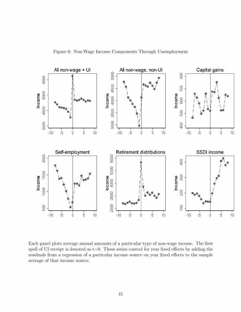
Figure 6: Non-Wage Income Components Through Unemployment

Each panel plots average annual amounts of a particular type of non-wage income. The firstspell of UI receipt is denoted as t=0. These series control for year fixed effects by adding theresiduals from a regression of a particular income source on year fixed effects to the sampleaverage of that income source.

41

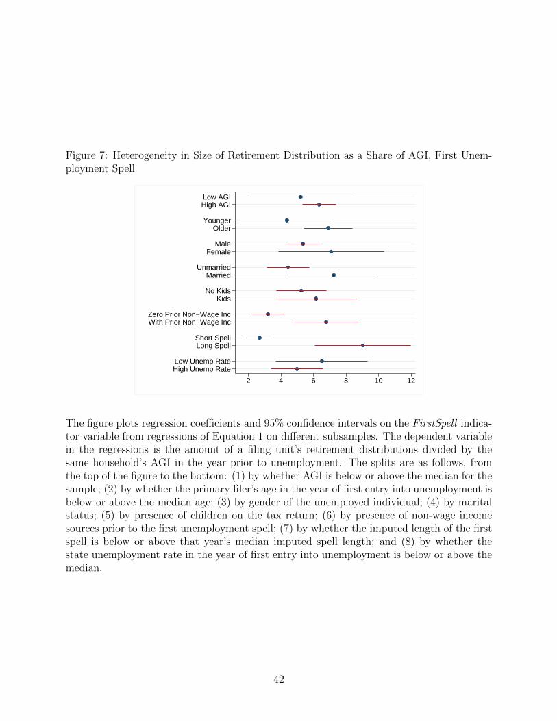
Figure 7: Heterogeneity in Size of Retirement Distribution as a Share of AGI, First Unem-ployment Spell

Low AGIHigh AGI

YoungerOlder

MaleFemale

UnmarriedMarried

No KidsKids

Zero Prior Non−Wage IncWith Prior Non−Wage Inc

Short SpellLong Spell

Low Unemp RateHigh Unemp Rate

2 4 6 8 10 12

The figure plots regression coefficients and 95% confidence intervals on the FirstSpell indica-tor variable from regressions of Equation 1 on different subsamples. The dependent variablein the regressions is the amount of a filing unit’s retirement distributions divided by thesame household’s AGI in the year prior to unemployment. The splits are as follows, fromthe top of the figure to the bottom: (1) by whether AGI is below or above the median for thesample; (2) by whether the primary filer’s age in the year of first entry into unemployment isbelow or above the median age; (3) by gender of the unemployed individual; (4) by maritalstatus; (5) by presence of children on the tax return; (6) by presence of non-wage incomesources prior to the first unemployment spell; (7) by whether the imputed length of the firstspell is below or above that year’s median imputed spell length; and (8) by whether thestate unemployment rate in the year of first entry into unemployment is below or above themedian.

42

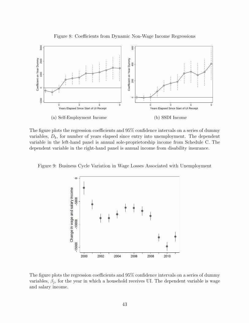
Figure 8: Coefficients from Dynamic Non-Wage Income Regressions−

1000

010

0020

0030

00

Coe

ffici

ent o

n Y

ear

Dum

my

0 3 6 9

Years Elapsed Since Start of UI Receipt

(a) Self-Employment Income

020

040

060

0

Coe

ffici

ent o

n Y

ear

Dum

my

0 3 6 9

Years Elapsed Since Start of UI Receipt

(b) SSDI Income

The figure plots the regression coefficients and 95% confidence intervals on a series of dummyvariables, Dk, for number of years elapsed since entry into unemployment. The dependentvariable in the left-hand panel is annual sole-proprietorship income from Schedule C. Thedependent variable in the right-hand panel is annual income from disability insurance.

Figure 9: Business Cycle Variation in Wage Losses Associated with Unemployment

The figure plots the regression coefficients and 95% confidence intervals on a series of dummyvariables, βj, for the year in which a household receives UI. The dependent variable is wageand salary income.

43

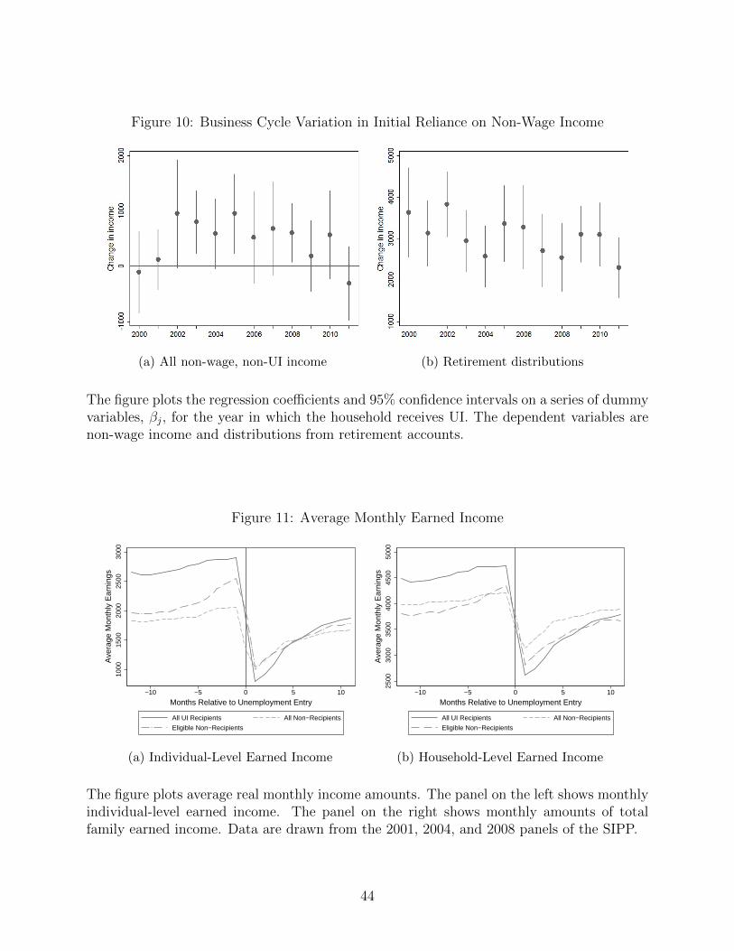
Figure 10: Business Cycle Variation in Initial Reliance on Non-Wage Income

(a) All non-wage, non-UI income (b) Retirement distributions

The figure plots the regression coefficients and 95% confidence intervals on a series of dummyvariables, βj, for the year in which the household receives UI. The dependent variables arenon-wage income and distributions from retirement accounts.

Figure 11: Average Monthly Earned Income

1000

1500

2000

2500

3000

Ave

rage

Mon

thly

Ear

ning

s

−10 −5 0 5 10

Months Relative to Unemployment Entry

All UI Recipients All Non−Recipients

Eligible Non−Recipients

(a) Individual-Level Earned Income

2500

3000

3500

4000

4500

5000

Ave

rage

Mon

thly

Ear

ning

s

−10 −5 0 5 10

Months Relative to Unemployment Entry

All UI Recipients All Non−Recipients

Eligible Non−Recipients

(b) Household-Level Earned Income

The figure plots average real monthly income amounts. The panel on the left shows monthlyindividual-level earned income. The panel on the right shows monthly amounts of totalfamily earned income. Data are drawn from the 2001, 2004, and 2008 panels of the SIPP.

44

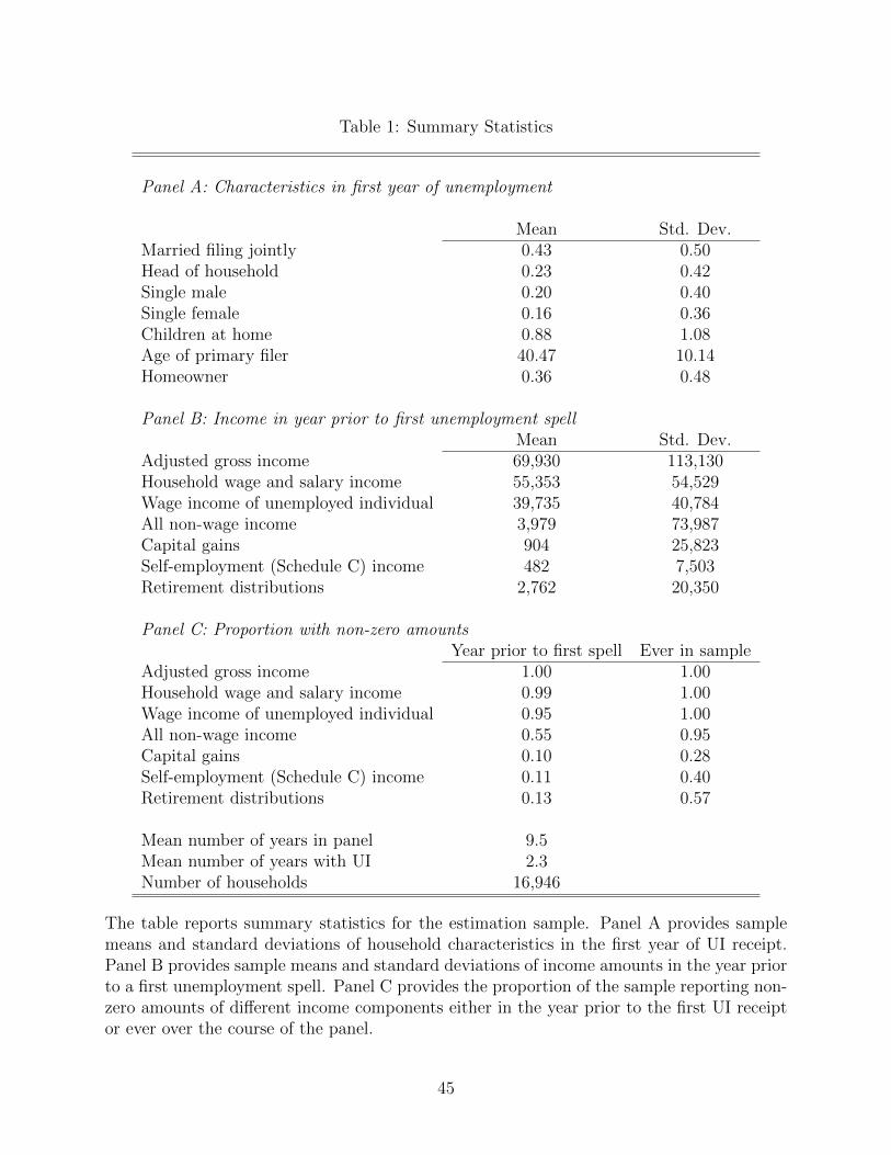
Table 1: Summary Statistics

Panel A: Characteristics in first year of unemployment

Mean Std. Dev.Married filing jointly 0.43 0.50Head of household 0.23 0.42Single male 0.20 0.40Single female 0.16 0.36Children at home 0.88 1.08Age of primary filer 40.47 10.14Homeowner 0.36 0.48

Panel B: Income in year prior to first unemployment spellMean Std. Dev.

Adjusted gross income 69,930 113,130Household wage and salary income 55,353 54,529Wage income of unemployed individual 39,735 40,784All non-wage income 3,979 73,987Capital gains 904 25,823Self-employment (Schedule C) income 482 7,503Retirement distributions 2,762 20,350

Panel C: Proportion with non-zero amountsYear prior to first spell Ever in sample

Adjusted gross income 1.00 1.00Household wage and salary income 0.99 1.00Wage income of unemployed individual 0.95 1.00All non-wage income 0.55 0.95Capital gains 0.10 0.28Self-employment (Schedule C) income 0.11 0.40Retirement distributions 0.13 0.57

Mean number of years in panel 9.5Mean number of years with UI 2.3Number of households 16,946

The table reports summary statistics for the estimation sample. Panel A provides samplemeans and standard deviations of household characteristics in the first year of UI receipt.Panel B provides sample means and standard deviations of income amounts in the year priorto a first unemployment spell. Panel C provides the proportion of the sample reporting non-zero amounts of different income components either in the year prior to the first UI receiptor ever over the course of the panel.

45

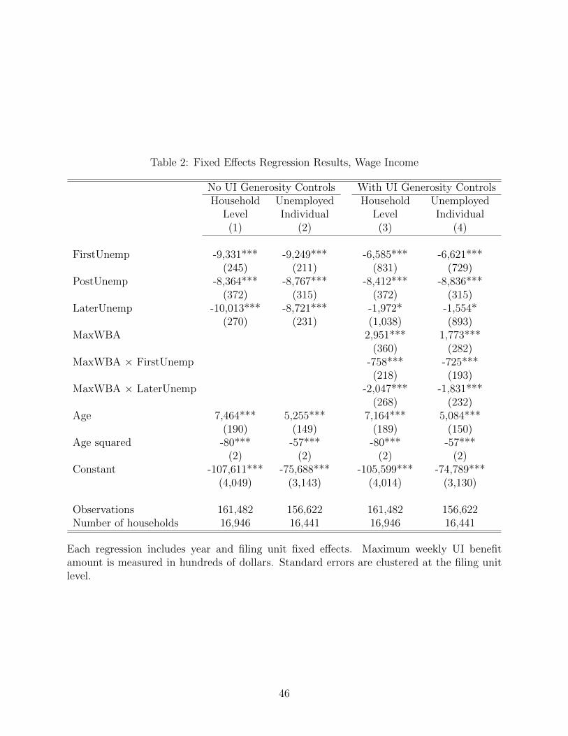
Table 2: Fixed Effects Regression Results, Wage Income

No UI Generosity Controls With UI Generosity ControlsHousehold Unemployed Household Unemployed

Level Individual Level Individual(1) (2) (3) (4)

FirstUnemp -9,331*** -9,249*** -6,585*** -6,621***(245) (211) (831) (729)

PostUnemp -8,364*** -8,767*** -8,412*** -8,836***(372) (315) (372) (315)

LaterUnemp -10,013*** -8,721*** -1,972* -1,554*(270) (231) (1,038) (893)

MaxWBA 2,951*** 1,773***(360) (282)

MaxWBA × FirstUnemp -758*** -725***(218) (193)

MaxWBA × LaterUnemp -2,047*** -1,831***(268) (232)

Age 7,464*** 5,255*** 7,164*** 5,084***(190) (149) (189) (150)

Age squared -80*** -57*** -80*** -57***(2) (2) (2) (2)

Constant -107,611*** -75,688*** -105,599*** -74,789***(4,049) (3,143) (4,014) (3,130)

Observations 161,482 156,622 161,482 156,622Number of households 16,946 16,441 16,946 16,441

Each regression includes year and filing unit fixed effects. Maximum weekly UI benefitamount is measured in hundreds of dollars. Standard errors are clustered at the filing unitlevel.

46

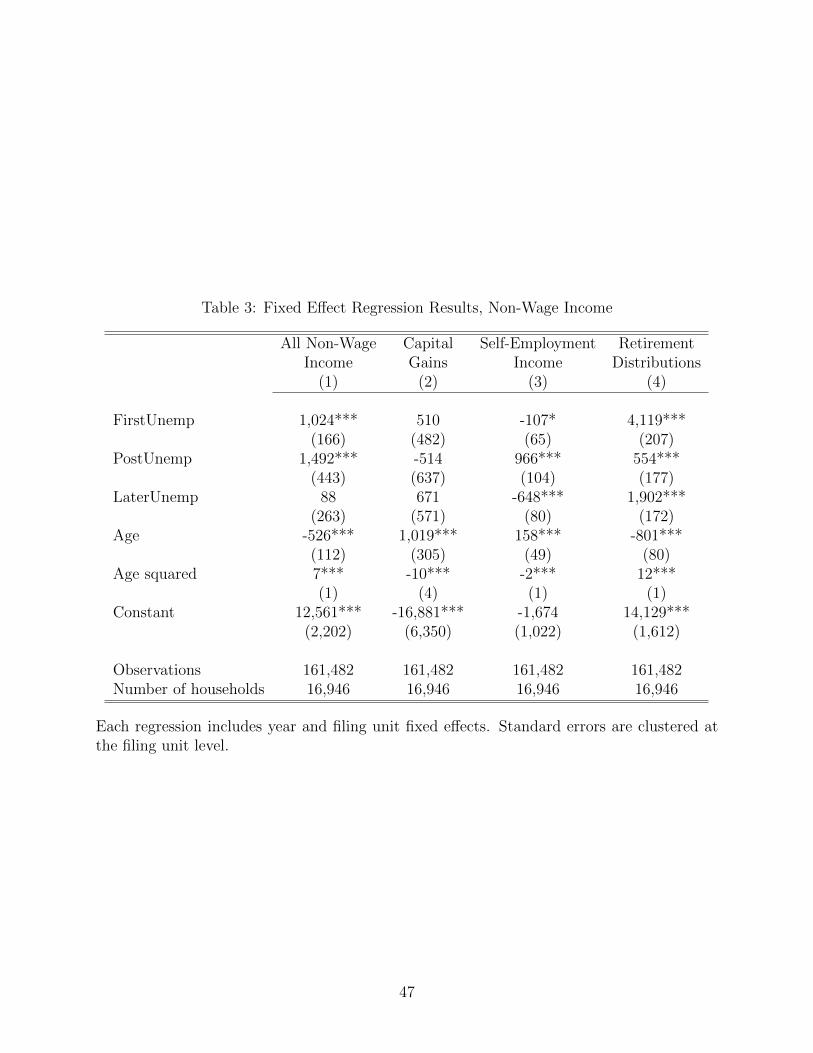
Table 3: Fixed Effect Regression Results, Non-Wage Income

All Non-Wage Capital Self-Employment RetirementIncome Gains Income Distributions

(1) (2) (3) (4)

FirstUnemp 1,024*** 510 -107* 4,119***(166) (482) (65) (207)

PostUnemp 1,492*** -514 966*** 554***(443) (637) (104) (177)

LaterUnemp 88 671 -648*** 1,902***(263) (571) (80) (172)

Age -526*** 1,019*** 158*** -801***(112) (305) (49) (80)

Age squared 7*** -10*** -2*** 12***(1) (4) (1) (1)

Constant 12,561*** -16,881*** -1,674 14,129***(2,202) (6,350) (1,022) (1,612)

Observations 161,482 161,482 161,482 161,482Number of households 16,946 16,946 16,946 16,946

Each regression includes year and filing unit fixed effects. Standard errors are clustered atthe filing unit level.

47

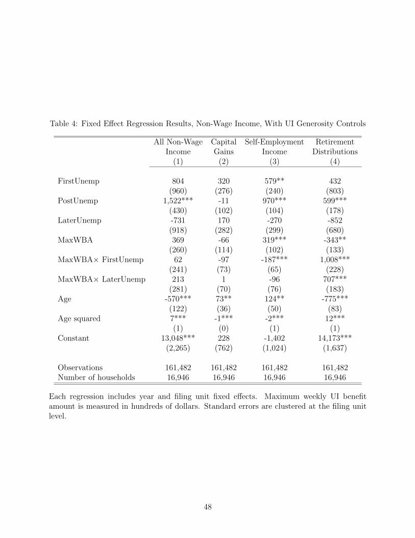
Table 4: Fixed Effect Regression Results, Non-Wage Income, With UI Generosity Controls

All Non-Wage Capital Self-Employment RetirementIncome Gains Income Distributions

(1) (2) (3) (4)

FirstUnemp 804 320 579** 432(960) (276) (240) (803)

PostUnemp 1,522*** -11 970*** 599***(430) (102) (104) (178)

LaterUnemp -731 170 -270 -852(918) (282) (299) (680)

MaxWBA 369 -66 319*** -343**(260) (114) (102) (133)

MaxWBA× FirstUnemp 62 -97 -187*** 1,008***(241) (73) (65) (228)

MaxWBA× LaterUnemp 213 1 -96 707***(281) (70) (76) (183)

Age -570*** 73** 124** -775***(122) (36) (50) (83)

Age squared 7*** -1*** -2*** 12***(1) (0) (1) (1)

Constant 13,048*** 228 -1,402 14,173***(2,265) (762) (1,024) (1,637)

Observations 161,482 161,482 161,482 161,482Number of households 16,946 16,946 16,946 16,946

Each regression includes year and filing unit fixed effects. Maximum weekly UI benefitamount is measured in hundreds of dollars. Standard errors are clustered at the filing unitlevel.

48

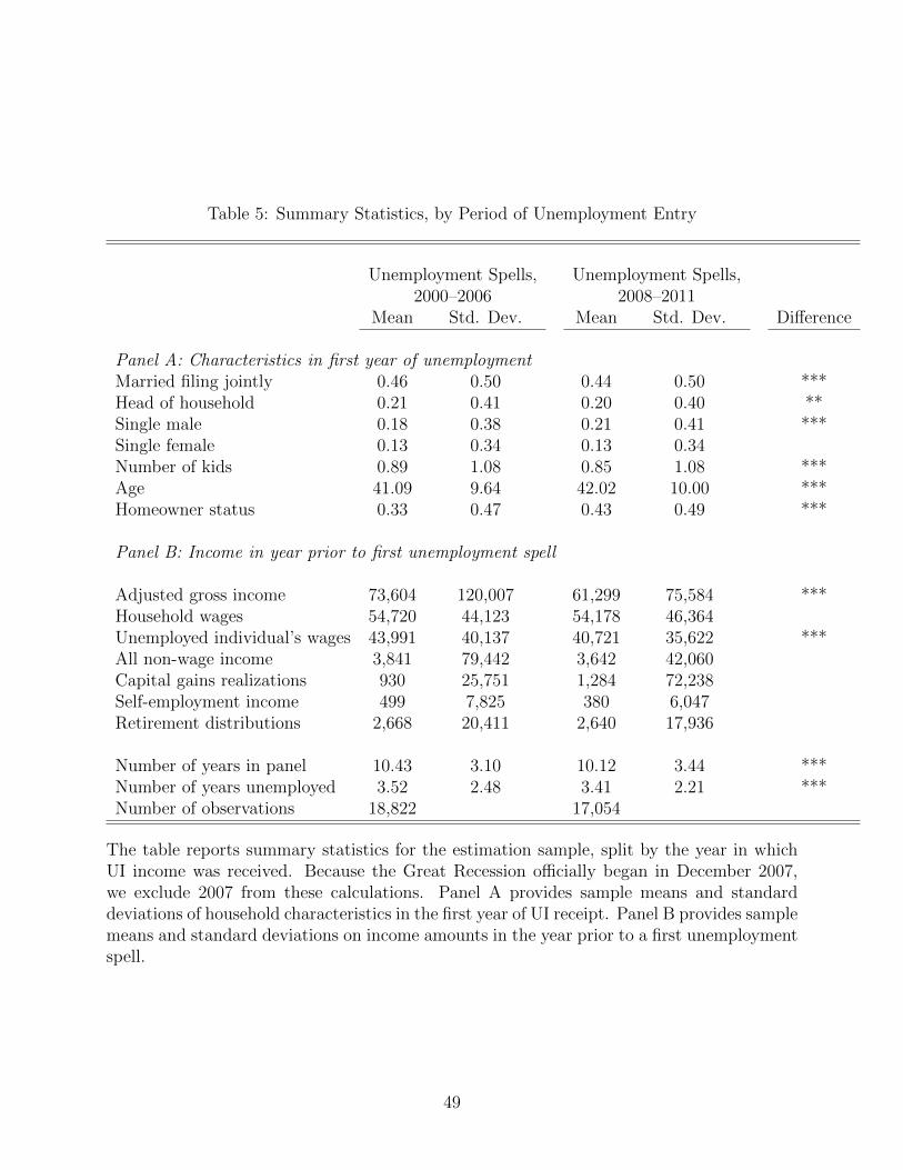
Table 5: Summary Statistics, by Period of Unemployment Entry

Unemployment Spells, Unemployment Spells,2000–2006 2008–2011

Mean Std. Dev. Mean Std. Dev. Difference

Panel A: Characteristics in first year of unemploymentMarried filing jointly 0.46 0.50 0.44 0.50 ***Head of household 0.21 0.41 0.20 0.40 **Single male 0.18 0.38 0.21 0.41 ***Single female 0.13 0.34 0.13 0.34Number of kids 0.89 1.08 0.85 1.08 ***Age 41.09 9.64 42.02 10.00 ***Homeowner status 0.33 0.47 0.43 0.49 ***

Panel B: Income in year prior to first unemployment spell

Adjusted gross income 73,604 120,007 61,299 75,584 ***Household wages 54,720 44,123 54,178 46,364Unemployed individual’s wages 43,991 40,137 40,721 35,622 ***All non-wage income 3,841 79,442 3,642 42,060Capital gains realizations 930 25,751 1,284 72,238Self-employment income 499 7,825 380 6,047Retirement distributions 2,668 20,411 2,640 17,936

Number of years in panel 10.43 3.10 10.12 3.44 ***Number of years unemployed 3.52 2.48 3.41 2.21 ***Number of observations 18,822 17,054

The table reports summary statistics for the estimation sample, split by the year in whichUI income was received. Because the Great Recession officially began in December 2007,we exclude 2007 from these calculations. Panel A provides sample means and standarddeviations of household characteristics in the first year of UI receipt. Panel B provides samplemeans and standard deviations on income amounts in the year prior to a first unemploymentspell.

49

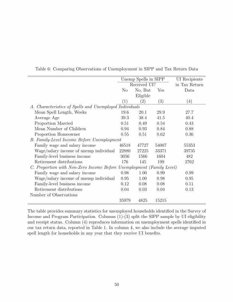
Table 6: Comparing Observations of Unemployment in SIPP and Tax Return Data

Unemp Spells in SIPP UI RecipientsReceived UI? in Tax Return

No No, But Yes DataEligible

(1) (2) (3) (4)A. Characteristics of Spells and Unemployed Individuals

Mean Spell Length, Weeks 19.6 20.1 29.9 27.7Average Age 39.3 38.4 41.5 40.4Proportion Married 0.51 0.49 0.54 0.43Mean Number of Children 0.94 0.93 0.84 0.88Proportion Homeowner 0.55 0.51 0.62 0.36

B. Family-Level Income Before UnemploymentFamily wage and salary income 46518 47727 54007 55353Wage/salary income of unemp individual 22880 27225 33371 39735Family-level business income 3056 1566 1604 482Retirement distributions 176 145 199 2762

C. Proportion with Non-Zero Income Before Unemployment (Family Level)Family wage and salary income 0.98 1.00 0.99 0.99Wage/salary income of unemp individual 0.95 1.00 0.98 0.95Family-level business income 0.12 0.08 0.08 0.11Retirement distributions 0.04 0.03 0.04 0.13

Number of Observations35979 4825 15215

The table provides summary statistics for unemployed households identified in the Survey ofIncome and Program Participation. Columns (1)-(3) split the SIPP sample by UI eligibilityand receipt status. Column (4) reproduces information on unemployment spells identified inour tax return data, reported in Table 1. In column 4, we also include the average imputedspell length for households in any year that they receive UI benefits.

50

A Data Appendix

Household wage and salary income: Household-level wage and salary income is reportedon line 7 on IRS Form 1040.

Individual-level wage and salary income: Wage income earned at each job is reportedon a W-2 form filed by the employer. We sum over all W-2s for each person in each yearto compute individual-level annual wage and salary income. For approximately 92% ofour sample, the difference between wages reported on the 1040 and wages derived fromW-2 filings is less than or equal to $25. There are several reasons why the wage andsalary amount reported on a filer’s tax return can differ from W-2 wages. The tax returnamount will be larger if the individual received scholarship or fellowship income, tipincome, certain employer-provided adoption benefits, or excess salary deferrals. TheW-2 amount will be larger if the individual is a statutory employee with business-related expenses to deduct. These individuals report W-2 amounts on Schedule C, noton the wage line of the tax return. For all tax filers not married filing jointly, we definewage income as the larger of the 1040-based amount and the sum of W-2 amounts. Fortax filers who are married filing jointly, we assign individual wages according to W-2records and split any positive difference between tax return earnings and combinedW-2 earnings equally between the primary and secondary filers.

All non-wage income: This composite measure is defined as total income (line 22 onForm 1040) less wage and salary income (line 7 on Form 1040) and UI benefits (line19 on Form 1040).

Capital gains realizations: Net capital gains is reported on line 13 on Form 1040 andis defined as the amount of taxable gains reported on the 1040, which aggregates long-term and short-term gains and losses. This variable can take on either positive ornegative values. Negative values occur when assets are sold at a loss. This measureincludes capital gains distributions paid out to holders of mutual fund shares. Thechoice of when to realize capital gains distributions from mutual funds is not withinthe control of the taxpayer, and thus will not be a particularly easy margin along whichto adjust during unemployment.

Self-employment income: Self-employment income is reported on line 12 on Form 1040and defined as net Schedule C income. These data likely only measure a portion of theactual involvement in self-employment. Some forms of temporary work may result inunder-the-table payments that are not reported to the IRS.

Gross distributions from retirement savings: Gross distributions from retirement sav-ings sums all withdrawals from IRAs (line 15a on Form 1040) and income from pensionsand annuities (line 16a on Form 1040).

Retirement penalty: The retirement penalty variable combines the 10% tax paid onany penalized early withdrawals from an IRA or employer-sponsored retirement plan(line 30 on Form 1040), as well as penalties paid on excess IRA contributions (line59 on Form 1040). Withdrawals from traditional IRA accounts generally trigger a

51

10% tax on the amount distributed if the IRA holder is under age 59.5. There area number of special cases under which an early IRA withdrawal is not subject tothe 10% penalty. Withdrawals used for first-time home purchases or for qualifiedhigher education expenses are exempt from the penalty. Most relevant for our analysis,withdrawals used to pay health insurance premiums are exempt for individuals whohave lost their jobs. Individuals who have held Roth IRAs for less than five yearsare subject to the same rules for early withdrawals as are holders of traditional IRAs,while those who set up a Roth IRA at least five years earlier are able to take tax-freewithdrawals at any time. Withdrawals from an employer-sponsored retirement plan,most often a 401(k), are typically subject to the 10% tax if the account holder is underage 55.

Social Security Disability Insurance (SSDI):

Although this income is not taxable, it is reported on the SSA-1099 information re-turns that the Social Security Administration provides to the IRS. This form does notdistinguish between payments made from different elements of the Social Security Ad-ministration’s Old Age and Survivor’s Insurance (OASI) and Disability Insurance (DI)programs. However, the age restrictions that we have imposed, 25 to 60, mean thateveryone in our sample is too young to be receiving Social Security retirement benefitsfrom OASI and too old to be receiving survivor benefits paid to children. This leavesSSDI payments and survivor benefits paid to widowed parents caring for children underage 16. Over the years that we analyze, SSDI payments account for more than 97%of these two types of payments. We have calculated this percentage using Social Se-curity Administration data from http://www.ssa.gov/oact/STATS/table4a4.html

and http://www.ssa.gov/oact/STATS/table4a5.html. We sum SSA-1099 paymentsto primary and secondary filers to get an aggregate measure of SSDI income for thehousehold.

Maximum Weekly Benefit Amount (MaxWBA):

The maximum weekly benefit amount available under the UI system is a summarymeasure of benefit generosity. Details on state programs come from the semi-annual“Significant Provisions of State Unemployment Insurance Laws” published by the De-partment of Labor’s Employment and Training Administration. Historical reportsare available at http://www.ows.doleta.gov/unemploy/statelaws.asp. States canchange their policies mid-year, and in cases where the January and July Departmentof Labor reports show different maximum benefit amounts, we use the simple averageof the two. A small number of states offer a larger maximum weekly benefit amountfor claimants with dependents. Results presented here use the benefit amount for afiler with no dependents, but we have checked that the patterns of results are robustto using the maximum weekly benefit amount including dependent allowances.

52

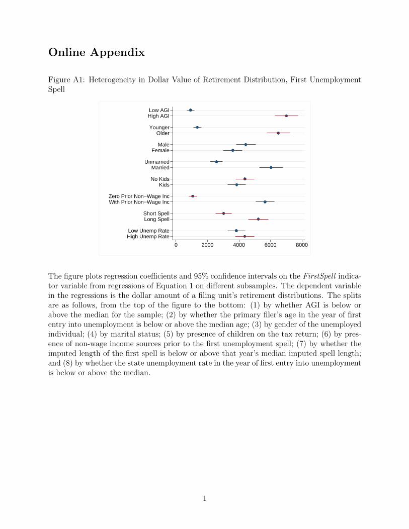
Online Appendix

Figure A1: Heterogeneity in Dollar Value of Retirement Distribution, First UnemploymentSpell

Low AGIHigh AGI

YoungerOlder

MaleFemale

UnmarriedMarried

No KidsKids

Zero Prior Non−Wage IncWith Prior Non−Wage Inc

Short SpellLong Spell

Low Unemp RateHigh Unemp Rate

0 2000 4000 6000 8000

The figure plots regression coefficients and 95% confidence intervals on the FirstSpell indica-tor variable from regressions of Equation 1 on different subsamples. The dependent variablein the regressions is the dollar amount of a filing unit’s retirement distributions. The splitsare as follows, from the top of the figure to the bottom: (1) by whether AGI is below orabove the median for the sample; (2) by whether the primary filer’s age in the year of firstentry into unemployment is below or above the median age; (3) by gender of the unemployedindividual; (4) by marital status; (5) by presence of children on the tax return; (6) by pres-ence of non-wage income sources prior to the first unemployment spell; (7) by whether theimputed length of the first spell is below or above that year’s median imputed spell length;and (8) by whether the state unemployment rate in the year of first entry into unemploymentis below or above the median.

1

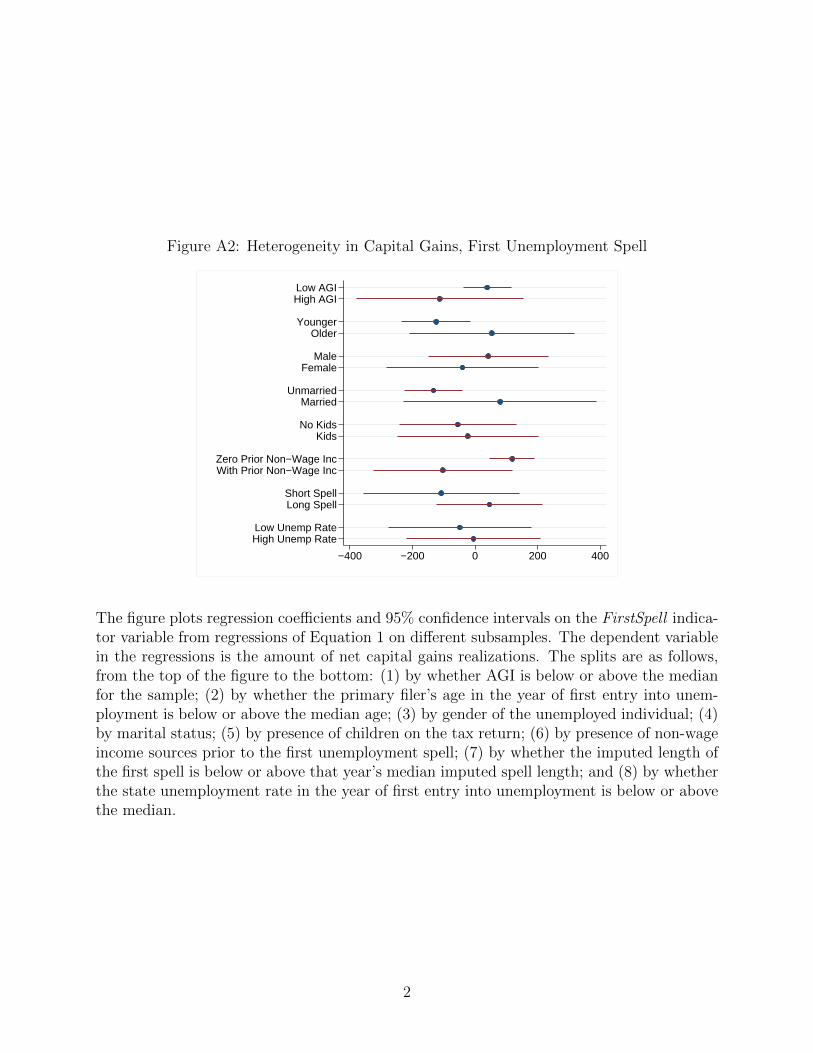
Figure A2: Heterogeneity in Capital Gains, First Unemployment Spell

Low AGIHigh AGI

YoungerOlder

MaleFemale

UnmarriedMarried

No KidsKids

Zero Prior Non−Wage IncWith Prior Non−Wage Inc

Short SpellLong Spell

Low Unemp RateHigh Unemp Rate

−400 −200 0 200 400

The figure plots regression coefficients and 95% confidence intervals on the FirstSpell indica-tor variable from regressions of Equation 1 on different subsamples. The dependent variablein the regressions is the amount of net capital gains realizations. The splits are as follows,from the top of the figure to the bottom: (1) by whether AGI is below or above the medianfor the sample; (2) by whether the primary filer’s age in the year of first entry into unem-ployment is below or above the median age; (3) by gender of the unemployed individual; (4)by marital status; (5) by presence of children on the tax return; (6) by presence of non-wageincome sources prior to the first unemployment spell; (7) by whether the imputed length ofthe first spell is below or above that year’s median imputed spell length; and (8) by whetherthe state unemployment rate in the year of first entry into unemployment is below or abovethe median.

2

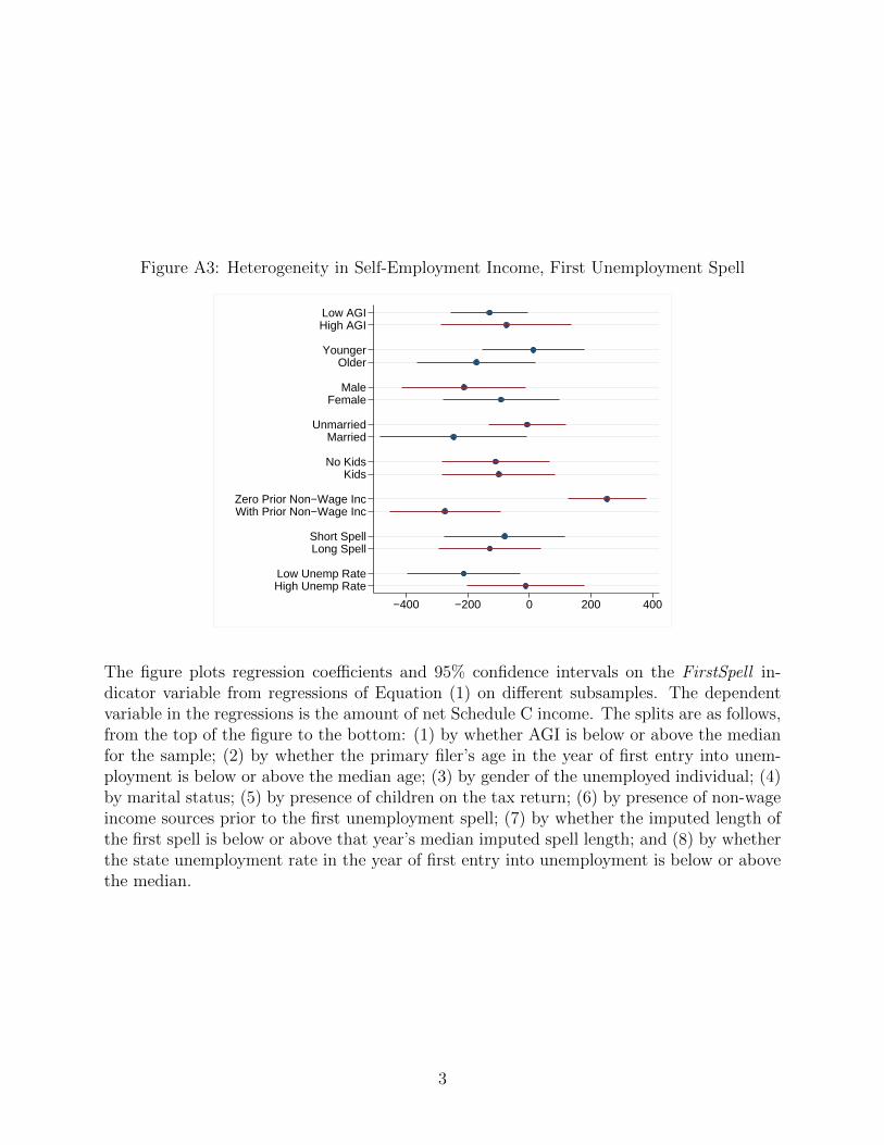
Figure A3: Heterogeneity in Self-Employment Income, First Unemployment Spell

Low AGIHigh AGI

YoungerOlder

MaleFemale

UnmarriedMarried

No KidsKids

Zero Prior Non−Wage IncWith Prior Non−Wage Inc

Short SpellLong Spell

Low Unemp RateHigh Unemp Rate

−400 −200 0 200 400

The figure plots regression coefficients and 95% confidence intervals on the FirstSpell in-dicator variable from regressions of Equation (1) on different subsamples. The dependentvariable in the regressions is the amount of net Schedule C income. The splits are as follows,from the top of the figure to the bottom: (1) by whether AGI is below or above the medianfor the sample; (2) by whether the primary filer’s age in the year of first entry into unem-ployment is below or above the median age; (3) by gender of the unemployed individual; (4)by marital status; (5) by presence of children on the tax return; (6) by presence of non-wageincome sources prior to the first unemployment spell; (7) by whether the imputed length ofthe first spell is below or above that year’s median imputed spell length; and (8) by whetherthe state unemployment rate in the year of first entry into unemployment is below or abovethe median.

3