Risk-based Selection in Unemployment Insurance:

Evidence and Implications

Camille Landais

LSE

Arash Nekoei

Stockholm University

Peter Nilsson

Stockholm University

David Seim

Stockholm University

Johannes Spinnewijn∗

LSE

November 11, 2020

Abstract

This paper studies whether adverse selection can rationalize a universal mandate for unem-

ployment insurance (UI). Building on a unique feature of the unemployment policy in Sweden,

where workers can opt for supplemental UI coverage above a minimum mandate, we provide the

first direct evidence for adverse selection in UI and derive its implications for UI design. We

find that the unemployment risk is more than twice as high for workers who buy supplemental

coverage. Exploiting variation in risk and prices, we show how 25-30% of this correlation is

driven by risk-based selection, with the remainder driven by moral hazard. Due to the moral

hazard and despite the adverse selection we find that mandating the supplemental coverage to

individuals with low willingness-to-pay would be sub-optimal. We show under which conditions

a design leaving choice to workers would dominate a UI system with a single mandate. In this

design, using a subsidy for supplemental coverage is optimal and complementary to the use of

a minimum mandate.

Keywords: Adverse Selection, Unemployment Insurance, Mandate, Subsidy

∗We thank Francesco Decarolis, Liran Einav, Itzik Fadlon, Amy Finkelstein, Francois Gerard, Nathan Hendren,Simon Jaeger, Henrik Kleven, Jonas Kolsrud, Neale Mahoney, Magne Mogstad, Emmanuel Saez, Frans Spinnewyn,Pietro Tebaldi, and seminar participants at Marseille, Stanford, Ecole Polytechnique, UCL, Cambridge, Bonn, Ein-audi, AEA Meetings, IFS, San Diego, NBER PF/Insurance Spring Meeting, Amsterdam, Zurich, CEPR Public PolicyMeeting, Wharton, BFI, Chicago Harris, and LSE for helpful comments and suggestions and our discussants AttilaLindner and Florian Scheuer for their valuable input. We also thank Arnaud Dyevre, Miguel Fajardo-Steinhauser,Alice Lapeyre, Will Parker, Yannick Schindler and Quirin von Blomberg for excellent research assistance. We ac-knowledge financial support from the ERC starting grants #679704 and #716485 and FORTE Grant #2015-00490.

1

1 Introduction

While unemployment insurance (UI) systems vary in many dimensions across countries (e.g., the

level and time profile of unemployment benefits), they share one striking similarity: employed

workers are mandated to participate in UI and are not given any choice. They are forced to pay

payroll taxes when employed and receive a set transfer when unemployed, which is not subject

to choice. Why do (almost) all countries mandate UI? Why is no coverage choice available? Are

these optimal features of UI design? Despite the large existing literature on UI, these fundamental

questions have so far been unanswered.

A universal mandate is seen as the canonical solution to the inefficiencies arising under adverse

selection [see Akerlof [1970], Chetty and Finkelstein [2013]]. Indeed, it is well-known that adverse

selection hinders efficient market function as low risks leave the market and put upward pressure

on equilibrium prices. While adverse selection is arguably the culprit in the context of UI, there are

two issues with this argument. First, since UI is universally mandated, the role of adverse selection

in UI cannot be directly tested. Second, even when adverse selection is present, the government

may do better by using alternative interventions that allow for choice. Our paper tries to address

both issues. We provide first-time evidence on the presence and severity of risk-based selection

into unemployment insurance and we develop a general framework to evaluate the desirability of a

universal mandate vs. choice-based interventions using this evidence.

We study this question in the Swedish context, where all workers are entitled to a minimum

benefit level when becoming unemployed, but can opt to buy more comprehensive UI at a uniform

premium set by the government. The combination of a mandate into basic coverage with a (subsi-

dized) option for more generous coverage is used in other Scandanivian UI programs and common

practice in other social insurance programs around the world.

We provide a theoretical framework - with both adverse selection and moral hazard - to evaluate

the design of social insurance programs allowing for choice. The policy levers in our framework are

the plan prices and coverage levels. When plan prices reflect the costs of individuals selecting those

plans, the concern is that workers will ‘under-insure’. In principle, both price and coverage levels

can be adjusted - with a universal mandate as an extreme case - to induce people to buy more

comprehensive coverage. The fiscal externality from steering workers from basic into comprehensive

coverage equals the difference between the price and cost differentials for workers at the margin.

This wedge will not only depend on how adversely selected plan choices are, but also on the moral

hazard response of these workers to the extra coverage. The fiscal externality for the marginal

workers needs to be compared to the welfare impact of the plan changes on the inframarginal

workers. We derive sufficient-statistic formulae, combining insights from the Einav-Finkelstein

[Einav et al. [2010b]] and Baily-Chetty [Baily [1978], Chetty [2006]] frameworks, that highlight the

central trade-offs and can be implemented empirically. In particular, we demonstrate how, on the

one hand, adverse selection in both the comprehensive and basic plan and, on the other hand,

moral hazard among workers on either the comprehensive or basic plan, are essential inputs to the

2

evaluation of the optimal price and coverage levels.

Our empirical analysis aims to provide estimates of these inputs, exploiting the combination of

the exceptional setting and rich administrative data in Sweden. In particular, we observe the UI

choice of the universe of Swedish workers and can link these choices to their unemployment histories

registered by the Public Employment Service. We also merge this data with a rich collection of

household and firm registers, providing extremely detailed information on the determinants of

workers’ unemployment risk and insurance choices. We present a set of empirical results, which

provide direct and robust evidence that workers have private information about their unemployment

risk, and act on this when making their unemployment insurance choice.

In a first step, we perform so-called positive correlation tests, assessing whether workers who

choose to buy comprehensive UI are more likely to be unemployed [see Chiappori and Salanie

[2000]]. Our estimates indicate that unemployment for workers buying the comprehensive coverage

is about 2.3 times more likely than for workers who choose to stay on basic coverage. This large

difference, however, reflects the combined impact of risk-based selection and moral hazard. To

separate the two, we build a rich predictive model of individuals’ ex ante unemployment risk,

leveraging various features of the Swedish labor market that provide variation in unemployment

risk beyond the direct control of individuals.1 Our decomposition implies that the difference in

ex post risk realizations driven by adverse selection is less than half of the wedge driven by moral

hazard. Moreover, the moral hazard response to supplemental coverage is estimated to be large

even for the workers who stick to basic coverage, unlike the “selection on moral hazard” findings

in Einav et al. [2013] and Shepard [2016].

In a second step, we provide direct evidence of risk-based selection following an approach in-

spired by Einav et al. [2010b], which consists in using price variation to identify marginal buyers

and compare their unemployment risk to inframarginal buyers of the same insurance plan. We

contribute to the standard approach by offering a methodology, based on panel data, that allows

for aggregate risk correlated with price variation. We exploit a large premium increase in 2007 and

find evidence of significant risk-based selection: the unemployment risk for the workers at the mar-

gin, who stopped buying comprehensive coverage when the price increased, is 20−40% higher than

for the inframarginal workers who did not buy comprehensive coverage, neither before nor after the

premium increase. Since their unemployment risk is measured under the same coverage, this differ-

ence cannot be driven by moral hazard. This difference in unemployment realizations between the

marginal and inframarginal workers disappears when conditioning on predictable unemployment

risk, which validates our earlier decomposition. In parallel to the price variation, we study how

changes in benefits affect demand and risk-based selection. We exploit the cap on the unemploy-

ment benefit level of the comprehensive plan in a regression kink design. Among the unemployed

workers, the share of workers on the comprehensive plan is increasing as the comprehensive benefit

level is higher, but their average unemployment risk is going down, providing additional evidence

1We also use these risk shifters more directly to test for the presence of risk-based selection, similar in spirit tothe unused observables test in Finkelstein and Poterba [2014].

3

of adverse selection.

In the final part of the paper we use our empirical estimates to evaluate a UI system with choice

of coverage:

First, despite the severe adverse selection, our estimates indicate that adverse selection by itself

cannot rationalize a universal mandate into comprehensive coverage in Sweden. The revealed value

for workers who choose not to buy the comprehensive coverage is exceeded by the insurance costs.

These costs are high due to the large estimated moral hazard response. As a result, mandating

those workers to buy the comprehensive coverage would decrease welfare. This is of course an

important conclusion in light of the universal mandates of comprehensive UI coverages in other

countries and the absence of prior tests whether adverse selection can make such policy desirable.2

Second, the estimated adverse selection indicates an important role for subsidizing comprehen-

sive coverage. Before the 2007 reform, the premium corresponded to only 31% of the difference

between the respective average costs of providing the comprehensive and basic plan. The large

subsidy encouraged around 86% of workers to buy the comprehensive plan. The 2007 price in-

crease eliminated this subsidy, but the demand response has been relatively inelastic. Our analysis

indicates that at the efficient price - at which the fiscal externality from encouraging workers to buy

comprehensive coverage is zero - still 83% percent of workers would buy it. The high pre-reform

subsidy, however, could still be rationalized by the redistributive gains away from workers on basic

coverage towards workers on comprehensive coverage.

Third, the optimal coverage differentiation crucially depends on the difference in moral hazard

costs. Our evidence suggests that for workers selecting the comprehensive coverage - who thus value

the extra coverage more - the moral hazard cost from providing the extra coverage is actually lower

than for workers selecting the basic coverage. This force suggests that maintaining a relatively large

difference in UI benefits across plans can be optimal. However, we note that these conclusions are

conditional on the level of prices: a decrease in the subsidy weakens the case for further coverage

differentiation. Put simply, a generous minimum mandate and a large subsidy for comprehensive

coverage are complementary policies.

Our work contributes to different strands of the literature. First, our work aims to contribute

to a large and rapidly growing empirical literature analyzing the role of adverse selection in in-

surance markets [see for example Einav et al. [2010a]], by highlighting the advantages of using

comprehensive, detailed and population-wide registry data and proposing new approaches to iden-

tify risk-based selection. Second, the lack of private markets and choices related to unemployment

insurance, makes that the role of adverse selection in UI specifically has been untested so far. Most

related to our paper is the work by Hendren [2017], who analyzes elicited beliefs about job loss

and finds that workers’ private information on their unemployment risk is sufficient to explain the

absence of a private market for supplemental unemployment insurance in the US (in addition to

the public UI policy in place). Our paper complements Hendren’s evidence with direct evidence

2Examples of countries mandating UI with similar replacement rates as the voluntary, comprehensive plan inSweden are Belgium, France, Luxembourg, Netherlands, Portugal, Spain and Switzerland. In other countries like theUS and the UK, UI is also compulsory, but at lower replacement rates.

4

based on actual insurance choices and studies the optimality of the public unemployment policy

itself. Finally, our work tries to bridge two strands of the social insurance literature, characterizing

optimal coverage policies under moral hazard [Baily [1978], Chetty [2006], Schmieder et al. [2012],

Kolsrud et al. [2018]] and characterizing optimal price policies under adverse selection [e.g., Hack-

mann et al. [2015], Tebaldi [2017], Finkelstein et al. [2019]]. Our conceptual framework provides

implementable insights for policy design, related to recent work by Veiga and Weyl [2016] and

Azevedo and Gottlieb [2017] who characterize equilibria with endogenous prices and coverages. In

comparison, we explicitly allow for moral hazard and potential selection on moral hazard like in

Einav et al. [2013] and Shepard [2016].

Our paper proceeds as follows. In Section 2 we describe the institutional background and the

data we use. Section 3 introduces our theoretical framework. In Section 4 we provide positive

correlation tests relating unemployment risk to UI coverage and decompose the positive correlation

between adverse selection and moral hazard using predictable risk. In Section 5 we use price

variation and benefit variation to provide evidence for risk-based selection and identify the statistics

necessary to identify the welfare consequences of various policy interventions. Section 6 puts things

together and determines the welfare impacts of various changes to the structure of the Swedish UI

system. Section 7 concludes.

2 Context and Data

2.1 Institutional Background

Sweden is with Iceland, Denmark and Finland, one of the only four countries in the world to have

a voluntary UI scheme, historically administered by trade union-linked funds (the so-called Ghent

system). This is the system many countries had in place before switching to compulsory insurance

overseen by the government [see Carroll [2005]]. The Swedish UI system consists of two parts:

The first part of the system is mandated and provides basic coverage funded by a payroll tax

(that we denote p0). The benefits that unemployed receive with this basic coverage (b0) are non-

contributory (i.e., do not depend on the unemployed earnings prior to displacement). The benefit

level of the basic coverage is low. During our period of analysis (2002-2009) the benefit level

remained at 320 SEK per day (≈35 USD) which corresponds to a replacement rate of a little less

than 20% for the median wage earner.3

The second part of the Swedish UI system is voluntary. By paying an insurance premium

p = p1 − p0 to UI funds (on top of the payroll tax p0), workers can opt for more comprehen-

sive coverage. Upon displacement, workers who have continuously contributed premia for the

comprehensive coverage during the past twelve months, get benefits b1, that replace 80% of pre-

unemployment earnings up to a cap, in lieu of the basic coverage b0.4 Apart from the benefit

3Benefits are paid per “working day”, which means that there are 5 days of benefits paid per week. Benefits of320 SEK a day therefore translate into 6960 SEK a month (≈765 USD).

4Enrolling in the supplemental coverage is done by filling out a form, which can be obtained online or in direct

5

level, there are no coverage differences between the basic and the comprehensive UI scheme. In

particular, the potential duration of benefits b0 and b1 is the same, and was unlimited during our

period of analysis. Moreover, to be eligible for either benefit upon unemployment, workers must

fulfil a labor market attachment criterion, which is that they need to have worked 80 hours per

month for six months during the prior year.5

The administration of the comprehensive UI coverage is done by 27 UI funds (so-called Kassa’s)

but the government, through the Swedish Unemployment Insurance Board (IAF), supervises and

coordinates the entire UI system. In particular, both the premia and benefit levels of the basic

and comprehensive coverage are fully determined by the government. To be clear, even though the

funds are in charge of implementing the system, they are all operating under the rules set by the

government, implying that Swedish UI is publicly provided.6 Importantly, the government does not

allow UI funds to charge different prices to different individuals. One exception are union members

who get a small rebate of ≈ 10% on the UI premium for the comprehensive coverage, so in our

empirical analysis, we always control for trade union membership to account for this.7 During our

period of study, the government also did not allow premia to differ across UI funds. Premia paid

by workers cover only a (small) fraction of benefits paid by the UI funds to eligible unemployed,

and the government subsidizes UI funds for the difference out of the general budget.

Until January 1st of 2007, the monthly premium p for the comprehensive coverage was ho-

mogeneous across UI funds, at around 100 SEK, and a 40% income tax credit was given for the

premia paid. In January 2007, the newly elected right-wing government increased the premium

substantially and removed the income tax credit on premia paid to UI funds. It also introduced an

additional fee that partly tied the premium of each UI fund to the average unemployment rate of

that fund, starting from July 2008. In our analysis, and partly due to data availability, we focus

on the period before July 2008 where insurance premia are homogeneous across UI funds.

The combination of a mandate into basic coverage with a (subsidized) option for more generous

coverage is not unique to the Swedish UI context, but commonly used in other social insurance

programs including health insurance, old-age pensions, disability insurance, etc. In the US health

contact with the UI funds. The premium is paid monthly and enrolled members can select between receiving monthlyinvoices or paying via direct debit. In case the fee is not paid for three consecutive months, despite monthly reminders,the membership is terminated (the neglected payments must still be paid). A cheaper way to opt out of the plan isto fill out a form, analogous to the procedure of opting in. There are no waiting periods associated with opting in orout, and the processing time for such requests are typically limited to a few days.

5Note that the self-employed are given the same option to get comprehensive coverage. To actually receive UIbenefits, they need to close their business [see Kolsrud [2018]]. In most countries, however, self-employed workers andthe growing share of workers under alternative work arrangements are not covered by the UI system - either becausethey don’t have access or are not mandated to participate [see OECD [2018]].

6Historically, with the “Ghent system” in place, labor and trade unions played an important role in providing unem-ployment insurance in Sweden. Today’s 27 UI funds, which broadly correspond to 27 different industries/occupations,originated from unemployment insurance funds set up by unions. However, since the government overtook the respon-sibility of supervising the entire UI system in 1948, the links between UI funds and unions have loosened progressively.

7The 10% rebate on UI premia for union members is a remnant of the “Ghent system”, but a large (≈ 20%) andgrowing share of workers are members of an unemployment fund without being members of a union, and a growingshare of union members (≈ 10%) do not buy unemployment insurance. Note that individuals can still continue tocontribute to UI funds while unemployed, for instance to build eligibility in case of a future unemployment spell, inwhich case they are also entitled to paying a reduced premium.

6

insurance market, for example, the recent Affordable Care Act involved the combined use of a

minimum mandate and subsidies. Social security design often combines public pension benefits

and tax-favored pension savings. To implement choice, a government may provide a menu of plan

options by itself, or alternatively provide or mandate only basic coverage and count on private

insurers to offer plans or top-ups.8

2.2 Data

We combine data from various administrative registers in Sweden. First, we use UI fund member-

ship information for the universe of workers in Sweden aged 18 and above, from 2002 to 2009, and

coming from two distinct sources. The first source is tax data for the period 2002 to 2006, during

which workers paying UI premia received a 40% tax credit. The UI funds sent information annually

to the Tax Authority about everyone who had contributed to the voluntary coverage plan within

the year. Our data contain the total amounts of UI premia paid for each individual and year, as

reported by the UI funds to the Tax Authority. From this source, we define a dummy variable D

for buying the comprehensive coverage in year t as reporting any positive amount of premia paid

in year t. For the analysis using the price variation of the 2007 reform in Section 5.1, we combine

this data with a second source of information, coming from UI fund data that Kassa’s sent to the

IAF. This data contain a dummy variable indicating whether an individual aged 18 and above in

Sweden is contributing premia for the comprehensive coverage as of December of each year from

2005 until 2009.

We add data on unemployment outcomes coming from the Swedish Public Employment Service,

with records for the universe of unemployment spells from 1990 to 2015, and we merge it with the

UI benefit registers from the IAF which provides information on all UI benefit payments (for

both the basic and comprehensive coverage), information on daily wage for benefit computation,

and Kassa membership information for all unemployed individuals. Based on this data, we define

unemployment as a spell of non-employment, following an involuntary job loss, and during which an

individual has zero earnings, receives unemployment benefits and reports searching for a full-time

job. To define the start date of an unemployment spell, we use the registration date at the PES. The

end of a spell is defined as finding any employment (part-time or full-time employment, entering a

PES program with subsidized work or training, etc.) or leaving the PES (labor force exit, exit to

another social insurance program such as disability insurance, etc.).9 We define displacement as an

involuntary job loss, due to a layoff or a quit following a ‘valid reason’.10 In the rest of the paper,

8See for example Cutler and Reber [1998] in the context of health insurance and Cabral and Cullen [2019] in thecontext of disability insurance.

9Note that UI benefits can be received forever in Sweden during the period 2002-2006 so the duration spentunemployed is identical to the duration spent receiving unemployment benefits.

10Valid reasons for quitting a job are defined as being sick or injured from working, being bullied at work, or notbeing paid out one’s wage by one’s employer. Quits are reviewed by the Public Employment Service at the momentan individual registers a new spell and if the quit is made because of a valid reason, the individual is eligible for UIand a notification is made in the PES data, allowing us to observe such quits under valid reasons. Involuntary quitsare a small fraction of unemployment spells in our sample: 95.0% of unemployment spells observed in our data aredue to layoffs. We exclude voluntary quits from our measure of unemployment and displacement.

7

we use the terms displacement and layoff as synonyms.

We complement the data with information on earnings, income, taxes and transfers and de-

mographics from the LISA register, and with information on wealth from the wealth tax registers.

We also exploit variation in unemployment risk across individuals due to Sweden’s employment-

protection law. In particular, we use the layoff-notification register (VARSEL) for years 2002 to

2012, which records the notifications by firms to the Public Employment Service as required by law

when intending to displace 5 or more workers. The list needs to follow the last-in-first-out (LIFO)

principle. For that, we use the matched employer-employee register (RAMS), from 1985 to 2015, to

compute tenure and tenure ranking for for the universe of individuals employed in establishments

of firms operating in Sweden.

2.3 Predictive Model of Unemployment Risk

We leverage the rich set of observables available in the Swedish registry data, and the various

institutional features of the Swedish labor market to build a predictive model of unemployment

risk. That is, the best predictor of future unemployment risk given all currently observed individual

characteristics. This measure will allow us to go beyond studying how realized risk in year t + 1

correlates with choice in t and also study how predictable risk in year t correlates with choices at

time t. This will prove important in separating adverse selection from moral hazard.

Our main measure of unemployment risk π throughout the paper, and the one relevant to the

UI system given insurance choices made in year t, is the number of days an individual is expected to

spend unemployed in t+1.11 To account for the fact that the distribution of days spent unemployed

is defined only over non-negative integers, and exhibits a significant mass at zero, throughout the

paper, we model π using a zero-inflated Poisson model. The expected number of days unemployed

conditional on a vector of characteristics X therefore takes the following form:

E(π|X) = (1− f(0|XI)) exp(X ′Cβ)

For the zero-inflated part of the process, we parametrize the probability f(0) using a logit: f(0|XI) =

exp(X ′Iβ)/(1+exp(X ′Iβ)). We will allow the set of risk predictors XI and XC , entering respectively

the inflated part and the count part, to differ.

The richness of the Swedish registry data allows us to observe many predictors of unemployment

risk such as age, education, location, occupation, industry, earnings, etc. The Swedish institutional

context also creates significant variation in unemployment risk that is arguably beyond the control

of individuals. In Appendix A, we present evidence showing the importance of three risk shifters

in particular, which will figure prominently in our vector X of risk predictors. The first risk shifter

is the average (i.e. “leave-out mean”) firm layoff rate. The second is layoff notifications: the risk

11If an individual has bought the comprehensive coverage throughout year t, then the days she spends unemployedin year t+ 1 will be covered by the comprehensive benefits. In that sense, the relevant risk to determine the cost ofproviding the comprehensive coverage to an individual buying that coverage in year t is the expected number of daysshe will spend unemployed in year t+ 1.

8

of unemployment increases significantly following layoff notifications. Finally, the enforcement of

the Last-In-First-Out principle creates significant variation in unemployment risk within firm over

time across individuals with different tenure levels.

In terms of model selection, we discipline the choice of the many potential regressors by using the

adaptive Lasso procedure for a zero-inflated Poisson model proposed by Banerjee et al. [2018], that

we detail in Appendix A.2. The regressors we allow to initially enter the model are individual log

earnings, family type, nine age bins, gender, twelve dummies for education level, year fixed effects,

region fixed effects, industry fixed effects, dummies for the past layoff history of the individual,

dummies for the layoff notification history of the firm, the leave-out mean of firm layoff risk, union

membership, tenure rank, interactions between tenure ranking and firm layoff risk and interactions

between tenure ranking and layoff notification history of the firm. The Lasso procedure ends up

mostly picking up the “institutional” risk shifters (i.e. layoff notification, tenure, etc.) in predicting

displacement risk, while other demographics such as education or region also play an important role

in the count part of the model. In Appendix A.2, we provide all further details on the estimation

procedure.

To account for moral hazard, we allow the risk of individuals with similar characteristics X to

differ if they are observed under the basic coverage or under the comprehensive coverage. To this

purpose, we estimate separately two models of predicted risk. The first model is the predicted risk

given X under the basic coverage π0 = E(π0|X). This model is estimated on individuals who are

observed under the basic coverage in t. The second model is the predicted risk given X under the

comprehensive coverage π1 = E(π1|X), which we estimate on individuals who are observed under

the comprehensive coverage in t.

To assess the quality of the model fit, Figure 1 shows bin scatters of the relationship between

predicted risk under basic (resp. comprehensive) coverage and actual realized risk for individuals

under basic (resp. comprehensive) coverage. In both panels, the relationship is close to the 45-

degree line indicating that the model does a good job at predicting the average realization of

unemployment risk. However, the model slightly under-predicts very long unemployment spells

for workers under comprehensive coverage (see Panel B). Comparing both panels, we also see that

individuals under basic coverage have lower realized unemployment risk, and thus lower predicted

risk than individuals in the comprehensive coverage. We provide additional elements of diagnostics

on the quality of our model fit and summary statistics on the distribution of predicted risk in

Appendix A.2. In general, we find significantly less dispersion in our predicted measure of risk

than in realized risk. This confirms that there still remains a substantial dimension of idiosyncratic

unemployment risk beyond what can be predicted even using a very rich set of observables.

2.4 Summary Statistics

In Table 1, we characterize the empirical setting by providing summary statistics for our main

sample of interest over the period 2002 to 2006. The sample consists of individuals aged between

18 and 60 and who have been working for at least 6 months. The average probability to be displaced

9

in year t + 1 conditional on working in year t is 3.0% over the period 2002 to 2006. The average

probability to be unemployed in year t+1 (unconditional on employment status in year t) is higher,

at 3.6%. The average (unconditional) number of days unemployed in t+ 1 is 5.28. Workers in our

sample are predicted to spend on average 3.57 days in t+1 if under the basic coverage and 5.83 days

if under the comprehensive coverage. Note also that the fraction of individuals who are members of

a UI fund (i.e., buying the comprehensive UI coverage) is large during the 2002-2006 period, at 86%.

The Table shows that there is also limited switching over time across coverages over the period

2002 to 2006. In Appendix Table B.3 we provide further summary statistics breaking down the

sample between individuals observed under the basic coverage and individuals observed under the

comprehensive coverage. The Table shows that individuals under the basic coverage are younger,

are more likely to be men and to be single, and hold significantly larger wealth and liquid assets

than individuals under comprehensive coverage.

3 Conceptual Framework

This section presents a conceptual framework that accounts for adverse selection and moral hazard

and underpins our empirical and welfare analysis. We first set up a model of UI choice in Sweden,

where a minimum benefit level is mandated, but workers can opt for comprehensive coverage. We

then use the framework to characterize the key trade-offs when setting prices and coverages as a

function of estimable moments. A universal mandate - with no choice offered - can be considered as

an extreme case of setting prices and/or coverages such that all individuals are on the same plan.12

3.1 Setup

Workers are offered the choice between two plans that differ in the coverage they provide against

unemployment risk: a basic plan (b0, p0) and a comprehensive plan (b1, p1). They can opt for

a higher UI benefit level b1 ≥ b0, but this comes at a higher price p1 ≥ p0. The coverages and

prices are the levers of the government’s unemployment policy. These policy levers affect workers’

selection of plans and their unemployment risk. The setup encompasses a universal mandate, when

(b0, p0) = (b1, p1) and no choice is allowed for.

The key micro-foundations for our analysis are workers’ plan valuations and the government’s

costs and how both change with the plans’ prices and coverage levels. Worker i chooses the plan

providing the highest utility ui (bj , pj). She will thus opt for the comprehensive plan when

ui (b1, p1) ≥ ui (b0, p0) . (1)

We will use short-hand notation u1, u0 and u = u1 − u0 respectively. A worker’s unemployment

risk depends on her type and the actions she undertakes given her coverage. For tractability, we

assume that workers’ preferences are quasi-linear in prices so that an individual’s risk, conditional

12See Appendix F for further discussion and proofs.

10

on plan choice j, does not depend on prices and neither does the ranking of individuals’ valuations

ui. Individual i’s unemployment risk under coverage bj is denoted by πi (bj) (or πj in short). The

average unemployment risk for workers who opt for coverage j if they are under plan j′ equals

Ej(πj′)

= E(πi(bj′)|ui (bj , pj) ≥ ui (b−j , p−j)

). (2)

The worker’s unemployment risk determines the cost to the government of providing coverage,

denoted by ci (bj) = πi (bj) bj .

3.2 Social Insurance Design

Our aim is to characterize how to set prices and coverages when both adverse selection and moral

hazard are present. Both forces have been the subject of large, but surprisingly parallel literatures

in social insurance. As is well known, adverse selection makes it inefficient to price insurance plans

at average cost, while moral hazard makes it inefficient to provide complete coverage.

We assume a concave and differentiable social welfare function,

W ≡∫ui≥0

ω (ui (b1, p1)) di+

∫ui<0

ω (ui (b0, p0)) di+ λ {F1 [p1 − E1 (π1) b1] + F0 [p0 − E0 (π0) b0]} ,

where the function ω (·) maps individuals’ utility into social welfare, λ equals the marginal cost of

public funds, which pre-multiplies the fiscal cost of the unemployment policy, and Fj denotes the

share of individuals buying plan j for given coverages and prices.

Our main focus is on the fiscal externalities of workers’ choices and how they change with

prices and coverages. We ignore the presence of other frictions or inefficiencies, but revisit later

the potential role of choice frictions due to behavioral biases [see Spinnewijn [2017]] and the ex-

ante value of insurance [see Hendren [Forthcoming]], which can both drive a wedge between the

welfare-relevant utility and the decision utility at the time a decision is made.

PCT Decomposition We first provide two complementary ways to quantify the respective

roles of adverse selection and moral hazard, which relate directly to the fiscal externalities from

changing the prices and coverage levels as derived below. Both adverse selection and moral hazard

increase the correlation between unemployment risk and coverage, E1 (π1)−E0 (π0). A first decom-

position of this PCT statistic is into the difference in risks for the two groups under comprehensive

coverage and the difference in risks under the two plans for the group selecting basic coverage,

E1 (π1)− E0 (π0) = E1 (π1)− E0 (π1)︸ ︷︷ ︸AS1

+ E0 (π1 − π0)︸ ︷︷ ︸MH0

. (3)

The former term captures adverse selection into the comprehensive plan (AS1), while the latter term

captures moral hazard for the group selecting basic coverage (MH0). The alternative decomposition

is into moral hazard for the group selecting comprehensive coverage (MH1) and adverse selection

11

into the basic plan (AS0),

E1 (π1)− E0 (π0) = E1 (π1 − π0)︸ ︷︷ ︸MH1

+ E1 (π0)− E0 (π0)︸ ︷︷ ︸AS0

. (4)

Differences in moral hazard among the individuals on comprehensive and basic coverage relate

mechanically to differences in adverse selection in the comprehensive and basic plan. Appendix

Figure F.1 provides a graphical illustration of these relations, linking this to the textbook analysis

of selection and treatment effects.13

Price Policy We now characterize the impact of a price change dpj on social welfare. We

consider a small deviation, so that we can invoke the envelope theorem: the impact on individuals’

welfare depends on the direct effect of the policy change, but not on the behavioral response and

re-sorting of individuals at the margin. The direct welfare effect of a price change dpj on the

buyers of plan j depends on the marginal social value of income for these workers, for which we use

short-hand notation Ej

(∂ωj∂pj

). This welfare effect should be compared to the fiscal impact of the

price change, which depends on both the direct revenue change dpj for the share of (inframarginal)

workers buying plan j and on the fiscal externality of the share of (marginal) workers switching in

or out of comprehensive coverage.

The fiscal externality due to the selection response depends on the difference between the price

differential p = p1 − p0 and cost of providing comprehensive instead of basic coverage to the

marginal buyers. This corresponds to the well-known result in Einav et al. [2010b]. Denoting the

unemployment risk of the marginal buyers by EM(p) (πj) = E (πj |u = 0), we obtain

FEASp ≡ [p1 − p0]−[EM(p) (π1) b1 − EM(p) (π0) b0

], (5)

=[E1 (π1)− EM(p) (π1)

]b1 +

[EM(p) (π0)− E0 (π0)

]b0 − S, (6)

where S = [E1 (π1) b1 − E0 (π0) b0] − [p1 − p0] denotes the subsidy for supplemental coverage cap-

turing how much the price differential differs from the average cost differential.

Equation (6) demonstrates how in our binary choice setting the fiscal externality accounts for

risk-based selection in both the comprehensive and basic plan. When both plans are priced at aver-

age cost and thus S = 0, adverse selection typically causes the fiscal externality to be positive. To be

more precise, if the marginal buyer is less risky than the average buyer of the comprehensive cover-

age and more risky than the average buyer of the basic coverage, the government will gain twice from

inducing this marginal buyer to switch from basic to comprehensive coverage.14 Approximating

13The differences in AS and MH generally relate to topics of heterogeneous treatment effects and selection intotreatment [e.g. Kowalski [2016]; Kline and Walters [2019]]. So-called selection on moral hazard [Einav et al. [2013]]can be interpreted as MH1 −MH0 > 0. The opposite can happen as well, but requires the difference in risks underbasic coverage to be larger than the difference in risks under comprehensive coverage, AS0 − AS1 > 0. Indeed,MH1 −MH0 = AS1 −AS0 immediately follows from decompositions (3) and (4).

14The expression for the fiscal externality in equation (6) also shows that selection and not moral hazard itselfdrives the inefficiency of average-cost pricing. The impact of moral hazard on the cost differential would be priced

12

E1 (π1)−EM(p) (π1) ≈ F1× [E1 (π1)− E0 (π1)] and EM(p) (π0)−E0 (π0) ≈ F0× [E1 (π0)− E0 (π0)],

the fiscal externality can be linked to the adverse selection terms in the PCT decompositions, (3)

and (4),

FEASp ≈ F1AS1b1 + F0AS0b0 − S, (7)

confirming that the fiscal externality depends on risk-based selection in both the comprehensive

and basic plan.15

Comparing the welfare effects from changing prices of the respective plans, we can state:

Proposition 1. For given coverage levels, the prices p0 and p1 are optimal only if

E1

(∂ω1∂p1

)E0

(∂ω0∂p0

) =1 + FEASp

∂ lnF1∂p1

1− FEASp∂ lnF0∂p0

.

The left-hand side of Proposition 1 captures the redistributive gain from transferring a marginal

dollar from individuals on the basic plan to those buying the comprehensive plan. The right-hand

side equals the fiscal return of these transfers due to the change in plan selection. For example,

a reduction in the premium for comprehensive coverage induces more workers to buy it and the

return to this selection effect is positive as long as the fiscal externality is positive (FEASp > 0).

In the absence of redistributive motives, the optimal subsidy is such that the fiscal externality

equals zero (FEASp = 0). The price differential then exactly reflects the cost of providing the

supplementary coverage to individuals at the margin. Increasing the subsidy further would cause

the fiscal externality to be negative (FEASp < 0), but could be justified by valuing redistribution

from workers on basic coverage towards workers on comprehensive coverage.

Coverage Policy We now turn to the impact of a change in coverage dbj . An increase in

coverage provides more insurance to the group of workers selecting this plan, but also reduces

their incentives to avoid unemployment. This standard trade-off between insurance and incentives

is captured by the well-known Baily-Chetty formula [Baily [1978], Chetty [2006]] applied to the

workers selecting a given plan.

Like in the Baily-Chetty formula, the fiscal externality of providing extra coverage depends on

the moral hazard response by these workers, captured by the increase in their unemployment risk

as coverage increases,

FEMHbj

= Ej

(∂πj∂bj

)bj

Ej (πj). (8)

However, a key difference with the standard Baily-Chetty formula comes from the extra fiscal gain

efficiently under average-cost pricing if the moral hazard impact were constant across workers.15The approximation would be exact under rank-linearity E (πj |u) = αj + βjG (u) for G(·) the cdf. This for

example holds when demand and cost curves are linear as in Einav et al. [2010b].

13

or cost due to the selection response to a coverage change. Like for a price change, we need to

account for the share of switchers into or out of comprehensive coverage. The corresponding fiscal

externality equals

FEASbj ≡ [p1 − p0]−[EM(bj) (π1) b1 − EM(bj) (π0) b0

], (9)

where EM(bj) (πk) = E(πk

∂uj∂bj|u = 0

)/E(∂uj∂bj|u = 0

)is a weighted average of the unemployment

risk among the marginal buyers under plan k. In comparison with the fiscal externality of a

price change FEASp , higher weight is given to the risk of the marginal buyers who value the extra

coverage more as they are more likely to switch.16 Of course, the coverage levels are no stand-

alone instruments and can be used in combination with subsidies. For example, setting a more

generous basic coverage level b0 will worsen the adverse selection into comprehensive coverage, but

the worsened adverse selection can be addressed with a more generous subsidy. In particular, a

higher subsidy will reduce the corresponding fiscal externality in equation (9).17

Comparing the welfare effects from changing coverages of the respective plans, we can highlight

the value of differentiating the coverages among which workers can choose:

Proposition 2. For given prices, the coverage levels b0 and b1 are optimal only if

E1

(∂ω1∂b1

)/E1 (π1)

E0

(∂ω0∂b0

)/E0 (π0)

=1 + FEMH

b1− FEASb1

∂ lnF1∂b1

/E1 (π1)

1 + FEMHb0

+ FEASb0∂ lnF0∂b0

/E0 (π0).

The left-hand side of Proposition 2 equals the ratio of the insurance gain from increasing the

coverage of the comprehensive vs. the basic plan. The value from extra coverage for workers on

either plan, Ej

(∂ωj∂bj

), depends on their marginal value from extra UI when unemployed.18 The

right-hand side equals the relative fiscal cost of increasing the coverages, depending on both the

moral hazard responses and the selection responses discussed above. The value of differentiating

the coverage levels b1 vs. b0 thus comes from the fact that individuals who value extra coverage

can opt for it. By revealed preference, we expect individuals who opt for extra coverage to value

it more, but the returns to differentiation are decreasing as workers are risk averse. The cost of

differentiating the coverage levels depends on how high the moral hazard cost is among workers

selecting comprehensive vs. basic coverage, but also on the fiscal return to encouraging more

individuals to opt for comprehensive coverage.

16The differential selection depending on plan characteristics has been studied for example in Veiga and Weyl[2016], but also relates to the difference in LATE’s depending on the instruments used [e.g., Kline and Walters[2019]; Mogstad et al. [2019]]. We show this formally in Appendix F.1. Note that if workers differ only along aone-dimensional index, the marginal buyers responding to a change in coverage or in price would be the same, aswould the corresponding fiscal externalities.

17The worsening selection in response to a generous minimum mandate has been studied before in Azevedo andGottlieb [2017] (see also Finkelstein [2004] and Chetty and Saez [2010]), but also provides a different perspective onthe absence of private UI (see Hendren [2017]), which is conditional on the mandated public UI that is already inplace.

18With expected utility and utilitarian social welfare, the scaled value term Ej(∂ωj

∂bj

)/Ej(πj) simplifies to the

average marginal utility of consumption when unemployed, just like in the standard expressions of the Baily-Chettyformula, but now for the workers on plan j.

14

Just like for the adverse selection externality, we can link the moral hazard externality back to

our earlier PCT decompositions,

FEMHbj≈MHj ×

bj[b1 − b0]Ej (πj)

.

Here we approximate the relevant marginal moral hazard response using the unemployment risk

response to a switch between comprehensive and basic coverage. This approximation indicates

that so-called selection on moral hazard (i.e., MH1 > MH0), where the moral hazard response is

larger for workers on comprehensive coverage, would weaken the argument for more differentiation.

Risk-based selection, however, either in the comprehensive plan (AS1) or in the basic plan (AS0),

would increase the fiscal return from inducing workers to switch to comprehensive coverage and

tends to strengthen the argument for more differentiation in coverage levels.

Universal Mandate Our analysis sheds light on the value of offering choice more generally.

The most common policy in the context of UI is to impose a universal mandate, not allowing

for any choice. The key question is whether introducing choice is desirable when starting from

a universal mandate. Or alternatively, when starting from a differentiated schedule, whether less

differentiation in coverages is desirable. Proposition 2 identifies the moments that allow answering

this question and helps deriving a simple non-parametric test to evaluate whether a universal

mandate into one of the coverage levels would be desirable. For example, we can evaluate the welfare

gains from a universal mandate into b1 by considering the corresponding coverage increase for the

workers under basic coverage. In line with the proposition, this is simply the sum of the insurance

gains net of moral hazard costs from the incremental coverage increases going from the basic to

comprehensive coverage, highlighting again that a potential impediment to mandating workers into

comprehensive coverage is moral hazard among those who value the comprehensive coverage the

least. Alternatively, we can consider a (sufficiently) large increase in p0 (or decrease in p1) such

that all workers under the basic plan switch to the comprehensive plan. In terms of efficiency

consequences, the conclusions are exactly the same. In line with Proposition 1, the efficiency gain

from such a universal mandate is simply the sum of the fiscal externalities ASp corresponding to the

required marginal price changes. Following Einav et al. [2010b], this corresponds to the valuation of

the supplemental coverage to the workers under the basic coverage relative to the cost of providing

it. Using a standard revealed preference argument, we can bound the valuation of the supplemental

coverage for these workers from above by the price differential p1 − p0 (which they are not willing

to pay). Hence, the earlier PCT decomposition in (3) allows for a simple, non-parametric test

for the desirability of a universal mandate. Mandating all workers into comprehensive coverage is

inefficient if

p1 − p0 ≤ b1E0 (π1)− b0E0 (π0) , (10)

= (b1 − b0)E0 (π0) + b1MH0. (11)

15

This test again underlines the importance of the moral hazard among the buyers of basic coverage,

but it does set the redistributive consequences aside and also assumes the absence of other frictions

that may justify a universal mandate.

Empirical Implementation. In the next two sections we turn to the empirical identification of

the various AS and MH terms determining the desirability of a mandate, and the welfare conse-

quences of changes to the price and benefit of UI policies in the Swedish context. We proceed in

three steps. First, we start with positive correlation tests and propose a decomposition of the test

statistic using predictable risk, separating the AS and MH terms. This allows, under some testable

assumption, for the identification of the desirability of a mandate. We then use variation in price.

This allows to identify AS terms directly, and enables the validation of our decomposition between

AS and MH terms. With this evidence, the welfare consequences of changes to the price structure

can be evaluated. We finally focus on benefit variation, which enables the identification of demand

responses to coverage levels and of AS for individuals at the margin of benefit variation. With this

evidence, the welfare consequences of changes to the benefit structure can be evaluated.

4 Positive Correlation Tests

A natural first step to investigate adverse selection is to produce correlation tests. We therefore

start by showing the presence of a strong positive correlation between an individual’s choice of UI

coverage and her unemployment risk. But correlation tests cannot disentangle the respective role of

adverse selection and moral hazard. Using our predicted risk model, we then show the presence of a

positive correlation between UI choices and predictable risk. These correlations confirm the presence

of significant adverse selection in both the basic (AS0 > 0) and comprehensive coverage (AS1 > 0).

We then use predictable risk to propose a decomposition of the positive correlation between selection

and moral hazard, the validity of which depends on a testable assumption. This decomposition

also allows for the identification of MH0, the moral hazard cost created by individuals who would

be moved to the comprehensive coverage by a mandate.

4.1 Positive Correlation Tests in Realized Risk

The correlation test consists in comparing the expected risk of individuals conditional on their

insurance coverage choice. In particular, we test for E1(π1|Z) > E0(π0|Z), where the vector

Z controls for characteristics that affect the unemployment insurance contracts available to an

individual.19 Over our baseline period of interest (2002-2006), UI contracts only differ according

to three dimensions.

19Controlling for these characteristics guarantees that we compare individuals who are facing the same options sothat the correlation is driven by demand rather than by supply (different individuals being offered different contractsby the Kassa). As explained in Section 2.1 above, characteristics affecting the premia and benefits under eachcoverage are strictly regulated by the government.

16

The first dimension is employment history. Coverage depends on whether individuals meet a

work eligibility requirement or not, for which they need to have worked for at least 6 calendar

months within the past 12 months prior to displacement. We therefore include in vector Z an

indicator for having worked at least 6 months in year t.20

The second dimension of contract differentiation is earnings. As explained in section 2.1, due

to the presence of a benefit cap, the additional daily benefits b ≡ b1− b0 that individuals get when

buying the supplemental coverage is a kinked function of daily earnings w. Formally, b = F (w) =

(.8 ∗w− 320) · 1[400 ≤ w < 850] + 360 · 1[850 ≤ w]. We therefore include the supplemental benefit

function F (w) as a control function in Z to make sure that we compare individuals facing the same

benefit level per unit of premium paid.

The last dimension of contract differentiation is that union members pay a slightly lower pre-

mium than non-union members for the supplemental coverage. We therefore include in Z an

indicator variable for union membership. We also include year fixed effects in Z to account for

small adjustments to the premium in January every year over the period 2002-2006.

To test in practice for E1(π|Z) > E0(π|Z), we use our baseline measure of risk π, which is the

total duration (in days) spent unemployed in year t + 1. And we correlate this measure of risk

with insurance choices made in year t. In practice, we estimate the following zero-inflated Poisson

process specification:

E(π|Z) = (1− f(0|Z,D)) exp(Z ′β + α · 1[D = 1]), (12)

where D ≡ δ(u ≥ 0) is an indicator for buying the comprehensive coverage.21 We estimate

specification (12) on the pooled sample of all individual i × year t observations between 2002 and

2006.

The first bar of Figure 2 reports the semi-elasticity of days unemployed in t+ 1 with respect to

insurance choice in t, estimated from model (12):

SemiPCT =E(π|Z,D = 1)− E(π|Z,D = 0)

E(π|Z,D = 0). (13)

Results indicate a strong and significant positive correlation between realized risk and UI coverage

choice: Individuals who buy the comprehensive coverage in t spend 135% more days in unemploy-

ment in t + 1 than individuals who stick to the basic coverage in t. Our results are robust to the

use of alternative measures of unemployment risk and to functional form specifications, as shown

in Appendix B.

20Note that eligibility requires individuals to have worked at least 80 hours per month for 6 calendar months withinthe past 12 months. While we do not have precise data on monthly hours, to be conservative, we also include adummy for having earnings above 80 hours × 6 months × the negotiated janitor wage. In the absence of an official,legally binding minimum wage in Sweden, the janitor wage is often considered the effective minimum wage in thelabor market.

21As explained above, the bolded notation ui refers to the difference in expected indirect utility between plan 1and plan 0 for individual i.

17

4.2 Selection on Predictable Risk

The predicted risk model presented in section 2.3 allows us to test how much UI coverage choices

correlate with predictable risk at time t, rather than realized risk at t + 1. This approach is akin

to the “unused observables” test of Finkelstein and Poterba [2014], and provides evidence that the

PCTs are not just driven by moral hazard but also by risk-based selection.

In the spirit of that test, we first gauge how the selection into coverage depends on specific insti-

tutional risk shifters, which enter the predicted risk model and are arguably beyond the control of

individuals. In Appendix C, we show that UI coverage choice is strongly correlated with average firm

layoff risk in the cross-section. Moreover, using a firm switcher design, we find that the probability

to buy comprehensive UI increases significantly when moving to a firm with a higher turnover risk.

Finally, within a firm, workers are more likely to start buying the comprehensive coverage when

the layoff risk increases as proxied by the firm’s sending of a layoff notification to the PES, and this

effect is strongest among individuals with lower relative tenure within occupation×establishment

cells, as predicted by the application of LIFO rules. The identifying variation and affected workers

differ for the three strategies, but the large and significant responses of UI coverage choice indicate

significant risk-based selection into UI.

By using the predicted risk model, we can leverage the variation in predictable risk in a com-

prehensive way and study the corresponding adverse selection. We use our baseline sample over

the period 2002-2006, and follow a specification similar to (12). We start by using as an outcome

the risk measure π0, which corresponds to the unemployment risk (in days) that an individual is

predicted to face in t+ 1 given her characteristics in t, were she to be under the basic coverage in

t. Results are presented in Figure 2. The second bar of the graph reports the semi-elasticity of π0

with respect to insurance choice defined in (13). It reveals that the group of individuals observed

choosing the comprehensive coverage in t are predicted to have ≈ 30% more days unemployed in

t+ 1 than individuals who do not buy, if both groups were hypothetically observed under the same

basic coverage.

We then turn to using π1 as an outcome, which corresponds to the unemployment risk predicted

under the comprehensive coverage. The third bar of Figure 2 reports the semi-elasticity of π1, with

respect to insurance choice in t. We find again a strong and significant positive correlation between

insurance choice and predicted risk. We note that the semi-elasticity of both measures of predicted

unemployment duration π0 and π1 are significantly smaller than the semi-elasticity for realized

unemployment duration in t+ 1 (first bar of Figure 2). As explained below, this difference can be

explained by the presence of significant moral hazard.22

4.3 Decomposition of PCT between Selection and MH

Under the assumption that there is no residual unobserved risk correlated with UI choice, all relevant

adverse selection in the basic and in the comprehensive coverage is identified by the difference in

22Appendix C provides further non-parametric evidence on the relationship between predicted risk and insurancechoice.

18

predictable risk between individuals observed in the comprehensive and in the basic coverage.

Formally, under the assumption that E1[π1|π1] = E0[π1|π1] (i.e., conditional on the predicted

risk, the average risk under comprehensive coverage is the same for both groups), selection in the

comprehensive coverage is:

AS1 ≡ E1 (π1)− E0 (π1) = E1 (π1)− E0 (π1) . (14)

Equivalently, under the assumption that E1[π0|π0] = E0[π0|π0] then selection in the basic coverage

is:

AS0 ≡ E1 (π0)− E0 (π0) = E1 (π0)− E0 (π0) . (15)

Importantly, the assumption underpinning (14) and (15) can be tested. In section 5.2, we use price

variation to identify willingness-to-pay, and we validate that there is no residual variation in risk

correlated with willingness-to-pay, when conditioning on our predicted risk measure.

Based on (14) and (15), we can get estimates of adverse selection into comprehensive (AS1)

and basic coverage (AS0) from our predicted risk model, and then use these estimates to provide

decompositions of the PCT, between selection and moral hazard. Following formula (3), we can

decompose the PCT between AS1 and moral hazard for individuals selecting into the basic coverage

MH0. Alternatively, we can decompose the PCT between AS0 and MH1, i.e., moral hazard for

individuals selecting into the comprehensive coverage, using formula (4).

We implement these decompositions in Figure 3 using our main sample over the period 2002-

2006, when on average 86% of individuals buy comprehensive coverage.

The decomposition shows large differences in predicted risk under comprehensive vs. basic

coverage. Despite the presence of significant adverse selection, most of the positive correlation

between risk and insurance choices is driven by moral hazard. The share equals 62 and 75 percent

respectively for the two alternative decompositions. The exercise also indicates the presence of

some small selection on moral hazard (i.e., MH1 > MH0), but that conclusion is reversed when

expressing the unemployment risk responses proportionally to the risk under basic coverage for

the respective groups (which is how the moral hazard terms enter the welfare characterizations in

Proposition 2).23 As stated before, the decompositions rely on the assumption that our predicted

risk model absorbs all variation in risk correlated with willingness-to-pay. If for instance, there

is adverse selection in the residual unemployment risk conditional on predictable risk, then, our

exercise will provide a lower bound on adverse selection, and an upper bound on moral hazard. We

now turn to using price and coverage variation to identify selection and we also use this to validate

our decomposition.

23The corresponding moral hazard elasticities are respectively .77 for individuals under comprehensive, and .94for individuals under basic coverage. The finding of substantive moral hazard is in line with the large literatureestimating the elasticity of unemployment durations/exit rates with respect to unemployment benefits: Schmiederand von Wachter [2016] summarize estimates from 18 studies from 5 different countries, and find a median of estimateof 0.53. Kolsrud et al. [2018] find an even larger elasticity of 1.53(.13) in the Swedish context.

19

5 Identifying Risk-based Selection using Plan Variation

In this section we exploit variation in both price and coverage levels to provide direct evidence

on risk-based selection, building on Einav et al. [2010b]. The selection effects determine the fiscal

externality of price and coverage interventions, following the welfare framework of Section 3. We

also use the price variation to test and validate the assumption underlying our earlier decomposition

between moral hazard and adverse selection.

5.1 The 2007 Price Reform

We first exploit a sudden and unanticipated increase in the premia paid to get the supplemental

coverage in 2007. The reform followed the surprise ousting of the Social Democrats from govern-

ment after the September 2006 general election. With this reform, monthly premia, which had been

remarkably stable over the previous years, suddenly increased from 100 SEK to around 320 SEK on

January 1st, 2007, as shown in Figure 4. The Figure also shows that the take-up of comprehensive

coverage responded significantly to this sharp surge in prices. After staying almost constant around

86%, the fraction of the eligible population buying the comprehensive coverage abruptly dropped to

78% right after the reform. Interestingly, Figure 4 displays little sign of pre-trends or anticipation

in the take-up rate of the comprehensive coverage, adding credibility to the assumption that this

sudden increase in premia, following the surprise change in political majority, was arguably exoge-

nous to individuals’ willingness-to-pay for the comprehensive coverage. The unemployment rate

was also smoothly decreasing throughout the period, so that the increase in p cannot be explained

by an endogenous pricing response to an increase in the underlying costs of the comprehensive

coverage.24

5.2 Risk-Based Selection Response to Prices

The 2007 reform created significant variation in price and in the fraction buying the comprehensive

coverage. Following Einav et al. [2010b], this variation could be exploited to identify adverse

selection by simply comparing average costs of providing comprehensive coverage across the different

price levels, i.e. before vs after the reform. Yet, in our context, variation in average costs may

also reflect realizations of some aggregate unemployment risk, which may vary over time, and will

therefore correlate with the price variation. More generally, if there is some aggregate component

to risk, and if there is correlation between aggregate risk variation and price variation, direct

comparisons of average costs across price observations as in Einav et al. [2010b] will not identify

adverse selection. This can be an issue in insurance contexts, where most of the variation in price

24If anything, the 2007 premia reform was combined with a minor legislated decrease in the benefits received in thecomprehensive coverage. On January 1st 2007, the cap on the benefits b1 was slightly decreased for benefits receivedin the first 20 weeks of an unemployment spell. Given this reform had only a negligible effect on average benefitsreceived, we neglect it in the welfare implementation.

20

available comes from variation over time, or across places and groups of individuals.25

We propose a simple method to address this issue and identify adverse selection. We use the

fact that with panel data, exogenous price variation allows for the identification of marginals, who

switch coverage in response to the price change. We can then rank individuals in three groups,

ordered in terms of their valuation of the supplemental coverage (u). First, we define group 1

as the group of individuals insured in the comprehensive coverage both in 2006 and 2007: they

were buying the supplemental coverage in 2006 under the low premia and continue to buy the

supplemental coverage under the high premia, and therefore have the highest valuation of the

comprehensive coverage (u > 0). We then define the group of marginals M(p), who were buying the

comprehensive coverage in 2006 but switch out in 2007 when premia p increase: these individuals

have a lower willingness-to-pay for supplemental insurance than individuals from group 1 and are

close to indifferent between the two coverages at current prices (u ≈ 0). Finally, individuals who

were neither buying the comprehensive coverage in 2006 nor in 2007, and are therefore always

under the basic coverage are defined as group 0: they have the lowest willingness-to-pay for the

supplemental coverage (u < 0).26

Using this ranking, we can now perform direct non-parametric tests for risk-based selection, by

correlating willingness-to-pay with measures of unemployment risk π. Because the marginals and

the individuals from group 0 are now observed under the same basic UI coverage, the comparison of

the average realized risk of these two groups under basic coverage (EM(p)(π0)−E0(π0)) is immune

to moral hazard and provides a direct estimate of risk-based selection.27 Because individuals

are compared under the same aggregate conditions, this test is also immune to aggregate risk

realizations correlated with the price variation.28

Figure 5 presents the results of such non-parametric tests and provides direct evidence of the

presence of risk-based selection into UI. Panel A starts by reporting the average number of days

spent unemployed in 2008 for each group. We condition again on the vector Z of controls for

contract differentiation, similar to what we did in the positive correlation tests. We define the

variable D as taking value 1 for group 1, M for marginals, and 0 for group 0. We then estimate

25For example, Hackmann et al. [2015] use price variation over time in the context of health insurance using adifference-in-differences design.

26Note that our partition of the population ignores a negligible fourth group of individuals, who were not buyingthe comprehensive plan in 2006, but switched in the comprehensive plan in 2007. The size of this group is seven timessmaller than the group of individuals switching out of the comprehensive plan in 2007. The reason we exclude thisgroup of workers from the analysis is that their ranking in terms of willingness-to-pay is ambiguous, as we discuss inAppendix D.

27It is worth re-emphasizing the timing of the Swedish UI policy: one needs to contribute for at least 12 months inorder to become eligible to the comprehensive benefits b1. Marginals and individuals from group 0 in 2007 did notcontribute any premium to the comprehensive plan in 2007. In 2008, if they become unemployed they will thereforeget the basic benefits b0 irrespective of their insurance choice in 2008. In other words, because of their insurancechoice in 2007, marginals and group 0 individuals face the exact same coverage in 2008. The difference in theirunemployment risk in 2008 cannot be driven by moral hazard due to different coverage choices in 2008.

28In a similar spirit, Shepard [2016]compares the costs of individuals staying and switching out of a plan in responseto a change in plan characteristics in the year before the change, when both groups were under the same plan.

21

specification:

Ej(π|Z) = (1− f(0|Z,D)) exp(Z ′β +∑j

αj1[D = j]). (16)

For each panel of Figure 5, we report E(π|Z = Z0, D = j), the average realized risk outcome π of

each group j = 1,M, 0, evaluated at the average value of Z for group 0.

Panel A shows that the average realized unemployment risk in 2008 of the marginals is signifi-

cantly higher (22%) than that of individuals who are always under the basic coverage, while both

groups are eligible to the same coverage in 2008. This is direct evidence of risk-based selection.

That is, a positive correlation between risk and willingness-to-pay for the supplemental coverage.

We can also see in panel A that there is a large and significant difference in the average realized risk

of the marginals and individuals from group 1. Because individuals from group 1 and the marginals

are now observed under different coverages, this difference identifies E1(π1) − EM(p)(π0) and is a

combination of selection and moral hazard.

In the last two panels of Figure 5, we report the relationship between willingness-to-pay and

predictable risk, using our predictive model of days spent unemployed. Panel B plots the average

predicted risk under basic coverage Ej(π0|Z) for the three groups j ∈ {1,M, 0}, where we use

the same method as in panel A to control for the vector Z of characteristics affecting contract

differentiation. Similarly, panel C plots the average predicted risk under comprehensive coverage

Ej(π1|Z) for the same three groups. Note that in both panels, we use the risk π0 and π1 predicted

by our model using individuals’ observable characteristics as of 2006.29 Comparing the predictable

risk of marginals individuals (j = M) to individuals with the lowest valuation of the comprehensive

coverage (j = 0), we find in both panels B and C the presence of significant adverse selection.

In Appendix D, we provide further results and probe into the robustness of our results. In

particular, we investigate the robustness to using alternative measures of risk and address poten-

tial concerns, such as inertia, to the validity of our ranking of individuals by willingness-to-pay.

We also provide additional results showing that our ranking of willingness-to-pay for the compre-

hensive coverage correlates strongly with determinants of the insurance value and proxies for risk

preferences.

Validation of PCT decomposition The evidence leveraging the price variation shows the

presence of significant adverse selection, but also suggests the presence of sizeable moral hazard. For

each group of workers - even those with the lowest willingness-to-pay for insurance - the predicted

unemployment risk is much larger in the comprehensive coverage than in the basic coverage, as

shown in the last two panels of Figure 5. Like for the decomposition of the PCT in section 4.3,

the separation between adverse selection and moral hazard requires that, once we condition on

our measure of predicted risk, there is no residual unobserved heterogeneity in risk correlated

with insurance choices. The price variation offers the possibility to test this assumption directly.

29We fix observable characteristics as of 2006, prior to the price change, as individuals might have changed thesecharacteristics endogenously in 2007 based on their new insurance coverage choice, which would reintroduce potentialmoral hazard. Fixing observable characteristics as of 2007 instead gives nevertheless very similar results.

22

Because we observe the risk under the basic coverage π0 of groups j = M and j = 0, we can test

for EM(p)(π0|π0) = E0(π0|π0).

Figure 6 displays the results. The left bar in the graph starts by reporting the difference in

realized risk in 2008 for the marginals (j = M) and for the individuals always in the basic coverage

(j = 0) when simply controlling for the vector of observables Z affecting the contract space. To

control for these observables, we use specification (16) above, and report on the graph:

SemiBaselineM(p) =E(π|Z,D = M)− E(π|Z,D = 0)

E(π|Z,D = 0),

This is the estimated semi-elasticity of the average realized risk under basic coverage for the

marginals M relative to the individuals always under basic coverage in 2006 and 2007.

To determine whether any correlation between risk and willingness-to-pay survives when con-

trolling for predicted risk, we now compute the residual semi-elasticity:

SemiResidualM(p) =EM(p)(π0|Z, π0)− E0(π0|Z, π0)

E0(π0|Z, π0),

where we condition on predictable risk by including in specification (16) twenty dummies for the

ventiles of predicted unemployment risk under basic coverage in both the inflated and count part

of the model.

Results, displayed in Figure 6, show that the semi-elasticity SemiResidualM(p) drops to a tightly

estimated zero when adding predicted risk as a control so that we cannot reject that EM(p)(π0|π0) =

E0(π0|π0). This evidence indicates that there is no significant residual correlation left between

realized risk and willingness-to-pay when we fully control for predicted unemployment risk using

the rich set of predictors from our predicted risk model. In other words, conditional on our predicted

risk score, if there remains any unobservable idiosyncratic component to risk, it is uncorrelated with

willingness-to-pay.

This result is particularly interesting. It suggests that little private information is left once

we condition on this very detailed set of proxies for unemployment risk. In the second column of

Figure 6, we investigate how much private information would be left if instead of controlling for

our predicted risk score, we controlled non-parametrically for a rich set of observable demographic

characteristics. We do so by including in specification (16) a set of dummies for age, gender, marital

status, education (four categories), industry (1-digit code) and wealth level (quartiles). Interest-

ingly, the semi-elasticity increases compared to our baseline when including these controls. This

suggests that these characteristics provide advantageous selection on average, such that if con-

tracts were differentiated along these observable dimensions, adverse selection into comprehensive

coverage would actually be more severe.30

30An important point to note is that when layoff decisions are mandated by rules at the govt level like theLIFO principle in Sweden, those rules can affect the extent to which unemployment risk depends on observable vs.unobservable charateristics. A corollary of this point is that the above result that observables capture all dimensionsof risk correlated with insurance choices in Sweden may not generalize to other labor markets like the US where firms

23

5.3 Regression Kink Design in UI Benefits

We now turn to variation in coverage levels and investigate the presence of adverse selection along

the benefit margin. To obtain benefit variation, we leverage the kinked schedule of UI benefits b1 in

the comprehensive plan as a function of pre-unemployment earnings. Workers in the comprehensive

plan receive daily unemployment benefits equal to 80% of their daily wage prior to unemployment,

up to a cap. Over the period 2002 to 2007, this cap in daily UI benefits was fixed at 680SEK,

meaning that the relationship between b1 and daily wage w exhibited a kink at w = 850SEK.31

We identify the effect of variation in b1 on demand and risk using a RK design, taking advantage

of the kinky schedule of b1 as a function of the daily wage. Our identifying variation is displayed

in Figure 7 panel A, which plots a bin-scatter of the relationship between the daily wage and

the observed average replacement rate for unemployed individuals in year t who have bought the

comprehensive coverage in t − 1 ∈ [2002; 2006]. The replacement rate is computed as the average

benefit received during unemployment from the IAF data divided by the daily wage. The graph

shows first that the replacement rate for b1 is close to exactly 80% on the left hand side.32 The

graph also displays a clear kink at w = 850SEK, with the replacement rate declining sharply,

as benefits are capped. We use this kinked relationship and treat it as a fuzzy RKD around the

850SEK threshold.

To implement this RK design, we use a measure of the daily wage coming from the IAF data.

Unfortunately, this measure is only available for individuals who become unemployed, and for whom

the IAF has to systematically collect this information to determine daily UI benefits. There does

not exist a corresponding measure of the daily wage for the universe of workers in the registry

data. For this part of the analysis, we therefore restrict our sample to individuals who become

unemployed in year t ∈ [2003; 2007] and were employed in year t − 1. For these individuals, we

relate their daily wage in year t − 1 to their insurance choice in t − 1 as well as their predictable

risk in t − 1. A consequence of this sample restriction is that individuals in this sample have a

higher average risk than in our original sample, as riskier individuals in t− 1 are more likely to be

observed unemployed in t (see Appendix Table E.2). We note however that this does not affect the

internal validity of our quasi-experimental analysis within this sample.

The key identifying assumption of the RK design is the existence of a smooth relationship at the

threshold w = 850SEK between the assignment variable and any pre-determined characteristics

affecting the demand for insurance. We assess the credibility of this assumption by conducting two

types of analysis in Appendix E. Considering the probability density function of the assignment

variable, we do not detect lack of smoothness around the kink that would indicate the presence of

selection. However, we find limited selection along observable characteristics around the kink, but

show robustness of our results when controlling for the corresponding vector of characteristics X.

have more flexibility in determining who they let go.31A daily wage of 850SEK corresponds to about 468USD a week using the average exchange rate over the period

2002 to 2007 of 1SEK ≈ 0.11USD.32Note that the reason why the replacement rate is slightly below 80% is that some workers have their UI benefits

reduced due to sanctions.

24

Like for the price variation, we first show that the demand for comprehensive coverage responds

positively to the level of UI benefits b1 offered in the comprehensive plan. Our RK estimand of the

demand response is given by:

δ =limw− dE[D|w]/dw − limw+ dE[D|w]/dw

limw− dE[b1|w]/dw − limw+ dE[b1|w]/dw, (17)

where D is, as in section 4 above, an indicator variable for buying the comprehensive coverage. We

estimate the numerator of the estimand based on the following specification:

D = β0 · (w − k) + β1 · (w − k) · 1[w > k] + Z ′γZ +X ′γX , (18)

where the coefficient β1 corresponds to the numerator in (17). The vector Z controls, as before,

for the characteristics that affect the premium paid for the comprehensive coverage over the period

2002 to 2006. It includes a dummy for union membership, a dummy for eligibility based on past

employment history, and year fixed effects.

Figure 7 panel B provides a graphical representation of our results, using a bandwidth of

350SEK. It plots the average fraction of individuals who bought the comprehensive coverage in a

given year, by bins of daily wage in that year. The relationship exhibits a sharp and significant

downward kink at the w = 850SEK wage threshold, which mirrors the sharp downward kink in the

relationship between daily wage and benefits in panel A. This indicates that the demand for the

comprehensive coverage responds negatively to a decline in the level of benefits b1 in that coverage.

We report on the graph the corresponding estimate of β1 ∗ 100 = −.016(.001) along with its robust

standard error. Based on the Delta-method, we obtain from this estimate a 95 % confidence interval

for the elasticity of comprehensive coverage with respect to benefits ∂1−G(0)∂b1

· b11−G(0) ∈ [.13; .19].

5.4 Risk-Based Selection Response to Coverages

We now test for the presence of adverse selection along the benefit margin. Like with adverse

selection along the price margin, we expect the marginals, who opt out of the comprehensive

coverage as benefits b1 decrease, to have lower risk π1 in the comprehensive coverage than the

individuals who stay in the comprehensive coverage: E1(π1) > EM(b)(π1). Hence, a direct test

for adverse selection in the comprehensive coverage a la Einav et al. [2010b] is therefore that the

average risk of individuals in the comprehensive coverage goes up in response to the decrease in

demand for comprehensive coverage at the kink. Formally, we test for a significant positive change

in slope at w = k in the relationship between the daily wage and the average risk in comprehensive

coverage of the individuals observed in that coverage.

To implement this test, we conduct a RK analysis using our predicted risk measure π1 under

comprehensive coverage, which we first residualize on the same vectors Z and X as in (18).33 Panel

33As in sections 4 and 5 above, we use a zero-inflated Poisson structure to model the role of covariates Z and Xon risk πi, i ∈ {0, 1}:

E(πi|Z,X) = (1− f(0|Z,X)) exp(Z′γZ +X ′γX).

25

D of Figure 7 plots the relationship between the daily wage and the average residual risk measure˜π1 = π1 −E(π1|Z,X) among individuals in the comprehensive coverage.34 The panel suggests the

presence of adverse selection: the average predicted risk in the comprehensive coverage is somehow

flat as a function of daily wage on the left-hand side of the kink, but does increase significantly on

the right hand side, kinking upwards around w = 850. To formalize the test, we collapse ˜π1 at the

daily wage bin level, and run the following RK specification:

˜π1 = β0 · (w − k) + β1 · (w − k) · 1[w > k] (19)

using the number of observations per bin as analytical weights. We report the estimate of 100∗β1 =

.279 (.109) on the panel, which confirms the existence of a significant positive change in slope. We

obtain from these estimates a 95 % confidence interval for the elasticity of the average predicted

risk in the comprehensive coverage w.r.t to b1: ∂E[π1]∂b1

· b1E[π1] ∈ [.07; .48].

These results indicate that individuals do adversely select in the comprehensive coverage in

response to benefit variation. The average cost of providing the comprehensive coverage is therefore

decreasing as we expand the share of individuals in that coverage through increasing benefits b1,

which is important for evaluating the welfare impact of changing coverages, following Proposition

2.

We can replicate this analysis for the average risk under the basic coverage. Risk-based selection

implies that marginals switching into the basic coverage at the kink are riskier than individuals

who were already in the basic coverage: EM(b)(π0) > E0(π0). Panel C of Figure 7 plots the

relationship between the daily wage and the average residual risk measure ˜π0 = π0 − E(π0|Z,X)

among individuals in the basic coverage. Despite the lack of precision, due to the much more limited

number of individuals observed in the basic coverage, the graph does indicate again the presence

of an upward kink with an estimated change in slope: 100 ∗ β1 = .204 (.144).

In Appendix E, we further investigate the robustness of our results. We show that our estimates

are stable across bandwidth choices. We also document that the inclusion of the controls X has

little effect on the overall results. Finally, we perform permutation tests for inference, using placebo

kinks a la Ganong and Jager [2018], and confirm the presence of significant adverse selection.

6 Policy Implications

This section uses our empirical estimates to evaluate the policy instruments introduced in Section

3. In particular, the Swedish setting allows us to test for the first time whether adverse selection

can rationalize a generous UI mandate, which is commonplace in other countries. We also leverage

our estimates to evaluate the fiscal externalities from changing the price and coverage levels.

34For readability, we rescale the residual by the average predicted risk at the average values for covariates Z andX of individuals at the kink (w = k). So formally, the panel plots: π1 − E(π1|Z,X) + E(π1|Zw=k, Xw=k).

26

Universal mandate The high replacement rate in the comprehensive plan in Sweden is com-

parable to the replacement rates of UI mandates in many other countries, especially in Europe. As

shown in Section 3, we can test for the desirability of mandating all workers into the comprehen-

sive coverage by comparing the price of the extra coverage to its cost for workers choosing basic

coverage. To that purpose, we obtain cost estimates by converting the predicted days spent unem-

ployed (in Figure see Figure 5) using E0 (cj) = E0(πj) · bj for both plans j = 1, 0.35 The difference

between the two gives an estimate for the cost of providing the extra coverage of 1, 712SEK to

workers choosing the basic plan. This estimate reflects the large predicted moral hazard response

when these workers opting for basic coverage would be put under comprehensive coverage. In

comparison, before the 2007 reform in Sweden, workers had to pay a net premium of 720SEK

per year, accounting for the 40 percent tax credit. By revealed preference, this provides an upper

bound on the valuation of workers opting for basic coverage, which is nevertheless substantially

below the corresponding costs. As these workers value the coverage less than it costs, their choice

not to buy comprehensive coverage is efficient. Imposing a universal mandate that forces them to

buy the comprehensive coverage would be inefficient. This observation, reflecting the strong moral

hazard response for workers with low valuation, raises the question whether a universal mandate

of generous UI coverage observed in many other countries is socially desirable.

Setting Prices While a universal mandate may not be desirable, prices can still be used to

overcome adverse selection by encouraging more workers into comprehensive coverage. Before the

price increase in 2007, comprehensive coverage was heavily subsidized with the premium paying for

only 31% of the difference in average costs. To calculate the fiscal externality form inducing workers

to buy comprehensive coverage instead of basic coverage, following Proposition 1, we construct

cost curves in the spirit of Einav et al. [2010b]. As discussed in Section 5, the price increase itself

identifies individuals at the margin between the two plans and allows us to study how the cost of

providing coverage changes with willingness-to-pay.

To construct cost curves, we convert the predicted risks (see Figure 5) into cost estimates, using

Ej(cj′)

= E0(πj′) · bj′ for the three groups of individuals j = 1,M, 0 and for both plans j′ = 1, 0.

We then position the three groups on the x-axis according to their willingness-to-pay, as shown

in Panel A of Figure 8. Individuals who choose the basic coverage (0) both in 2006 and 2007

have the lowest valuation and are on the right hand side, while individuals who always buy the

comprehensive coverage (1) are on the left-hand side of the graph. The marginals correspond to

the group in between, and their share is given in Figure 4, where we see the fraction of individuals

on comprehensive coverage dropping from 86 to 78% with the 2007 price increase. We then use

a linear extrapolation to obtain marginal cost curves for providing the comprehensive and basic

coverage respectively.36 Reflecting the earlier results on predicted risks, the cost of the marginals

35To account for the taxes paid on the unemployment benefits received, we scale down the costs by .20, whichcorresponds to the empirical average tax rate paid by the unemployed (see Kolsrud et al. [2018]).

36We locate the estimated costs for the three groups at the midpoint of the ranges of the corresponding valuationquantiles and then use a piece-wise linear interpolation to construct the cost curves. Appendix Figure F.2 plots

27

is in between the cost for those with higher and lower valuation, both under comprehensive and

under basic coverage.

We can now evaluate the fiscal externality from inducing workers to switch from basic to compre-

hensive coverage, i.e., the difference between the price and cost of providing supplemental coverage.

This is shown in Panel B of Figure 8. The black triangles correspond to the difference in costs from

providing the comprehensive and basic coverage, shown in Panel A. Providing the extra coverage

is on average more costly for the workers who value it more, but the extrapolation suggests that

for the group of switchers the cost stays between 1, 929SEK and 2, 051SEK.37 The grey triangles

show the pre- and post-reform prices and the corresponding take-up of comprehensive coverage.

By revealed preference, the valuation of the extra coverage for the group of switchers is bounded

between the pre-reform price of 720SEK and the post-reform price of 4, 116SEK. The difference

between revealed value and cost is negative for the marginal workers at the pre-reform price, indi-

cating that is was efficient for them to buy comprehensive coverage. The opposite is true at the

post-reform price. The fiscal externality is thus expected to be zero for some price in between.

Assuming a linear demand curve, as plotted in Panel B, the premium at which value and cost

coincide equals 2, 022SEK. 83 percent of workers would buy insurance at this efficient price.

While our estimates thus suggest that the large pre-reform subsidy induced too many individuals

to buy comprehensive coverage, setting the subsidy as high can be rationalized by valuing the

redistribution towards workers buying the comprehensive coverage. Evaluating the fiscal externality

per marginal worker FEASp at the pre-reform price, the right-hand side of Proposition 1 equals

1 + FEASp∂ lnF1∂p1

1− FEASp∂ lnF0∂p0

= 1.29,

using estimated price elasticities based on the demand response to the 2007 price increase (e.g.,∂ lnF0∂ ln p0

= .12, see Figure 4). Hence, the large pre-reform subsidy would be optimal if the return from

redistributing from workers under basic coverage to workers under comprehensive coverage equals

29%.38

Setting Coverages In Sweden the minimum UI benefit equals 320SEK (≈ 35USD) a day,

which is about half of the average benefit level under the comprehensive plan. Proposition 2

characterized the welfare impact from further differentiating these coverage levels, showing that

the corresponding risk curves under comprehensive and basic coverage and shows how comparable the realized vs.predicted risks are for the group of marginal buyers under basic coverage.

37Note the slope of this marginal cost curve - capturing the cost of providing supplemental coverage - does nolonger provide a test for adverse selection as in Einav et al. [2010b]. E.g., this curve can be upward sloping, whileboth the cost curve under comprehensive coverage and under basic coverage are downward sloping.

38Hendren [Forthcoming] proposes an approximation of the redistributive gain, given by E1

(∂ω1∂p1

)/E0

(∂ω0∂p0

)≈

1+ u′′(c)u′(c) × [p− E0 (p)], where the right-hand side depends on the curvature of utility in consumption and the average

willingness-to-pay for comprehensive coverage for those under basic coverage, E0 (p). Using the linear demand curve,the implied redistributive gain is less than 5% for CARA = 5 × 10−4 (expressing values in USD) or for CRRA = 3(for an average annual consumption level of 150, 000SEK).

28

the corresponding fiscal externality depends on two major forces.

The first force is the relative magnitude of the moral hazard costs, MHb1 and MHb0 , depending

on the unemployment risk response to a marginal change in the benefit level of workers who are

in the comprehensive and basic coverage respectively. We measure these two terms using the

arch-elasticity approximation:

FEMHbj≈MHj ×

bj[b1 − b0]Ej (πj)

.

where MHj is our estimate of the moral hazard response to a change in benefit from b0 to b1 for

individuals under coverage j. We find that: FEMHb0

= .94 > FEMHb1

= .77. In other words, the

moral hazard externality of increasing benefits at the margin is lower for individuals under the

comprehensive coverage than for individuals under the basic coverage. This force therefore pushes

in favor of differentiating the benefit coverages.

The second force shaping the fiscal externality in Proposition 2 comes from the selection re-

sponses. In an adversely selected market, we expect these selection responses to strengthen the

argument for benefit differentiation by decreasing the average risk of workers in both plans. Our

estimates in section 5.4 indeed suggest that an increase in the comprehensive coverage attracts

more workers in the comprehensive plan and reduces simultaneously the average costs of the com-

prehensive and of the basic plans. (A decrease in the benefit level of the basic coverage is expected

to do the same.) However, the fiscal externality depends not only on the risk-based selection re-

sponses, but also on the level of the subsidy for the comprehensive coverage (cf. formula (6)).

When the subsidy is high, the fiscal externality can be small or even negative despite significant

adverse selection, as the cost of providing the extra subsidy outweighs the gains from the decrease

in the costs of providing the coverages.

Evaluated again at the pre-reform price, we find that the fiscal externality of increasing the

coverage in the comprehensive plan relative to the basic plan equals:

1 + FEMHb1− FEASb1

∂ lnF1∂b1

/E1 (π1)

1 + FEMHb0

+ FEASb0∂ lnF0∂b0

/E0 (π0)≈ 1 + .77 + .06

1 + .94− .51= 1.27.

For this computation, we assume (i) that the demand response to a change in basic coverage is

the same as the response to a change in comprehensive coverage and (ii) that the switchers are the

same when considering variations in p, b0 or b1.39,40

The fiscal externalities in Proposition 2 need to be traded off against the relative consumption

39The first assumption can be formally stated as: ∂F1∂b1

/EM (π1) ≈ ∂F0∂b0

/EM (π0), evaluated for workers at the margin.This approximation would be exact under risk-neutrality.

40The second assumption always holds when the heterogeneity across agents can be captured by a one-dimensionalindex. The reason for relying on the second assumption is that we unfortunately lack power to credibly infer thepredicted risk for the marginal buyers with respect to the coverage levels from the RKD estimates of the change indemand and average costs, which are both imprecisely estimated. Assuming FEASb1 ≈ FEASb0 ≈ FEASp , we can useour fiscal externality estimates from the price variation exercise of section 5.

29

smoothing gains from extra coverages:E1

(∂ω1∂b1

)/E1(π1)

E0

(∂ω0∂b0

)/E0(π0)

. Further differentiation would therefore

be socially valuable if the marginal utility of an increase in benefits for individuals under the

comprehensive coverage is worth at least 27% more than the marginal utility of an increase in

benefits for individuals under the basic coverage. A back-of-the-envelope calculation based on recent

estimates from Landais and Spinnewijn [Forthcoming] in the same Swedish UI context suggests that

the value of extra coverage would be around twice as high for workers under comprehensive coverage

compared to workers under basic coverage, even when evaluated at b1 and b0 respectively.41 This

would imply that further differentiation in coverage levels enhances welfare and that providing the

right choice to workers also dominates a UI system with a single mandate.

Finally, we note that the welfare implications of coverage differentiation are conditional on

prices. At the current prices, the fiscal externality of inducing further individuals to switch to the

comprehensive coverage is negative because the subsidy is too generous. By the same token, the

selection response to a more generous minimum mandate would generate a positive fiscal external-

ity. Instead, when the subsidy were to be lowered, the resulting changes in the adverse selection

externalities would strengthen the case for further differentiation of the coverage levels.

Frictions and Timing of Choice Our welfare analysis has assumed that workers’ willingness-

to-pay for extra coverage reveals their valuation. We briefly discuss how choice frictions and the

timing of choice can affect the above policy implications.

First, choice frictions drive a wedge between workers’ willingness-to-pay and their welfare-

relevant valuation (Spinnewijn [2017]). For example, the workers choosing not take the compre-

hensive coverage may well underestimate its value. The price (720SEK) is only just above the

mechanical cost of providing the extra coverage (686SEK), not accounting for the cost increase

due to the unemployment response (i.e., E0(π0)[b1 − b0]). The pricing is thus close to - and for

the workers with lower risk better than - actuarially fair. One potential explanation why these

workers still choose not to buy is that they underestimate their unemployment risk or simply un-

derestimate the coverage they would get from comprehensive coverage.42 Another explanation is

that these workers over-estimate the price by not fully accounting for the 40% tax credit, but focus

on the before-tax premium of 1200SEK instead. If the revealed preference approach makes us

under-estimate the value of comprehensive coverage, the optimal subsidy should be higher and a

universal mandate may become desirable. Our findings, however, still imply that in Sweden the

severe adverse selection by itself is not sufficient to rationalize making the generous comprehensive

41In Appendix F we provide further detail on the evidence in Landais and Spinnewijn [Forthcoming] and thecorresponding back-of-the-envelope calculation, which crucially depends on two forces: heterogeneity in the value ofinsurance, conditional on risk, and diminishing marginal utility of consumption. People who buy the comprehensivecoverage b1 may do so because they value an additional kroner of consumption when unemployed more, conditionalon risk. However, diminishing marginal utility of consumption makes the value of an additional kroner lower whenevaluated at b1 than at b0.

42See Landais and Spinnewijn [Forthcoming] for more evidence and discussion on the role of risk perceptions inthis context, which is, however, inconclusive on the sign of the wedge between willingess-to-pay and welfare-relevantvaluation.

30

coverage compulsory. Moreover, given the large moral hazard response, the choice frictions have to

be substantial to change that conclusion.

Second, the presence of frictions may affect the estimated responses to changes in prices and

coverage.43 The 2007 reform increased the premium dramatically and, in fact, set it above the

difference in average cost of providing comprehensive and basic coverage respectively. While the

implied subsidy was thus eliminated, more than 3 out of 4 workers continued to buy comprehensive

insurance. Interestingly, this suggests that the inelastic demand could hold this adversely selected

market together when privatizing this market.44 The inelastic response may, however, be due to

inertia [e.g., Handel [2013], Polyakova [2016]]. To gauge this further, we study the insurance choice

of workers who switch firms and arguably face a more active choice environment. Appendix Figure

D.5 shows a comparable drop in demand for the comprehensive plan in the year after the premium

increase among firm switchers. The decrease in take-up extends to the next year among workers

who switch employers, while it flattens out for those who do not. We also investigated differences

in adverse selection for workers in a more vs. less active choice environment. Appendix Figure D.6

shows that the job switchers who switched out of comprehensive coverage in 2007 are again more

risky than the job switchers who were already in basic coverage in 2006. The semi-elasticities are of

comparable magnitude for those who switched employers and those who did not. While this does

not exclude the potential role of other frictions, it suggests that for the large 2007 reform inertia

has played a small role.

Third, related to choice frictions, the timing of choice may affect welfare calculations as well

(see Hendren [Forthcoming]). This will be particularly important in the presence of aggregate

risk, as this affects whether workers’ willingness-to-pay and their costs are sufficient to evaluate

welfare. The extent to which aggregate risk affects the identification of the welfare-relevant curves

depends on the timing of choice, that is, on the amount of aggregate risk that is realized at the time

individuals make their choice. From the cost side, if aggregate unemployment risk is not realized by

the time that individuals choose to buy insurance, using ex post realized costs rather than expected

cost at the time of insurance choice would bias the welfare conclusions. In our implementation, to

proxy for the expected cost at the time of the insurance choice in 2007, we use the predicted costs

based on our prediction model estimated on the 2002-2006 data. However, this would be a lower

bound on the expected cost if the increase in unemployment in 2008 at the start of the recession

was anticipated. From the demand side, if aggregate unemployment risk is realized by the time that

individuals choose to buy insurance, we would miss the ex-ante value of insurance against those

aggregate risks by using the observed willingness-to-pay. Incorporating this ex-ante value as in

Hendren [Forthcoming] would thus increase the average welfare-relevant value from extra coverage

43See Handel et al. [2019] for a welfare analysis that combines frictional demand and pricing inefficiencies due toadverse selection.

44As mentioned before, Hendren [2017] finds that adverse selection in the US context is sufficiently strong to explainthe absence of private insurance markets. In general, this prediction depends on the minimum mandate in place (seefootnote 3.2), which is more generous in the US than in Sweden. Note also that Hendren [2017]’s test does notaccount for other sources of heterogeneity that may reduce the correlation between risk and willingness-to-pay, whichwe show to be relevant in the Swedish context.

31

relative to the estimated demand curve.

7 Conclusion

Seventy five years ago, the Beveridge Report, in its attempt at increasing welfare for all, recom-

mended a new set of revolutionary social insurance policies and insisted that these insurance policies

“must be achieved by co-operation between the State and the individual. (...) The state should

not stifle incentive, opportunity, responsibility; in establishing a national minimum, it should leave

room and encouragement for voluntary action by each individual to provide more than that min-

imum for himself and his family”.45 In the context of unemployment insurance though, generous

mandates have left very little room for choice and voluntary actions by individuals, under the

(untested) presumption that offering choice would trigger risk-based selection. Our paper provides

the first direct evidence for risk-based selection into unemployment insurance and offers new in-

sights on how to reconcile social insurance design with individual choice in such a context of adverse

selection.

Using various empirical strategies and different sources of variation, we robustly find that work-

ers who face higher (ex-ante) unemployment risk select into more comprehensive coverage. Despite

the severe adverse selection, we find that mandating all workers into comprehensive coverage is not

the best policy response. The Swedish workers who choose not buy the comprehensive coverage

value it below its cost, which is high due to moral hazard. This is an important result, given an

ongoing policy debate in Sweden regarding a fully mandated unemployment insurance system, but

also given the universal mandates of comprehensive UI that are in place around the world – the

desirability of which has never been tested before. Moreover, the ubiquitous absence of private

markets for UI may be precisely because of the mandated public programs in place and the adverse

selection into supplemental coverage they cause. As our analysis shows, the impact of adverse se-

lection can be mitigated by subsidizing the premia for more comprehensive coverage, which would

increase the desirability of a more generous minimum mandate.

Importantly, the value of providing choice in social insurance programs does rely on individuals

using this choice in their best interest. This is an assumption we have maintained throughout to

focus our analysis. A rapidly growing literature documents the importance of frictions distorting

households’ insurance choices. This introduces another important caveat when introducing choice,

closely related to the potential for adverse selection. We leave this challenging, but important issue

for future research.

45Beveridge [1942]

32

References

Akerlof, George, “The Market for ‘Lemons’: Quality Uncertainty and the Market Mechanism,”

Quarterly Journal of Economics, 1970, 84 (3), 488–500.

Azevedo, Eduardo M. and Daniel Gottlieb, “Perfect Competition in Markets With Adverse Selec-

tion,” Econometrica, 2017, 85 (1), 67–105.

Baily, Martin N., “Some Aspects of Optimal Unemployment Insurance,” Journal of Public Eco-

nomics, 1978, 10 (3), 379–402.

Banerjee, Prithish, Broti Garai, Himel Mallick, Shrabanti Chowdhury, and Saptarshi Chatterjee,

“A Note on the Adaptive LASSO for Zero-Inflated Poisson Regression,” Journal of Probability

and Statistics, 2018.

Beveridge, William Henry, Social Insurance And Allied Services, HM Stationery Office London,

1942.

Cabral, Marika and Mark R. Cullen, “Estimating the Value of Public Insurance Using Complemen-

tary Private Insurance,” American Economic Journal: Economic Policy, August 2019, 11 (3),

88–129.

Carroll, Eero, “Voluntary State-Subsidized Social Insurance in the Advanced Industrialized World

since the 1890s: The Nordic Experience in Comparative Perspective,” in Olli Kangas and Joakim

Palme, eds., Social Policy and Economic Development in the Nordic Countries, London: Palgrave

Macmillan UK, 2005, pp. 60–87.

Chetty, Raj, “A General Formula for the Optimal Level of Social Insurance,” Journal of Public

Economics, 2006, 90 (10-11), 1879–1901.

and Amy Finkelstein, “Social Insurance: Connecting Theory to Data,” in Martin Feldstein Alan

J. Auerbach, Raj Chetty and Emmanuel Saez, eds., Handbook of Public Economics, Vol. 5 of

Handbook of Public Economics, Elsevier, 2013, chapter 3, pp. 111 – 193.

and Emmanuel Saez, “Optimal Taxation and Social Insurance with Endogenous Private Insur-

ance,” American Economic Journal: Economic Policy, May 2010, 2 (2), 85–114.

Chiappori, Pierre-Andre and Bernard Salanie, “Testing for asymmetric information in insurance

markets,” Journal of Political Economy, 2000, 108 (1), 56–78.

Cutler, David and Sarah Reber, “Paying for Health Insurance: The Trade-Off between Competition

and Adverse Selection,” The Quarterly Journal of Economics, 1998, 113 (2), 433–466.

Einav, Liran, Amy Finkelstein, and Jonathan Levin, “Beyond Testing: Empirical Models of Insur-

ance Markets,” Annual Review of Economics, 2010, 2, 311–336.

, , and Mark Cullen, “Estimating Welfare in Insurance Markets Using Variation in Prices,”

Quarterly Journal of Economics, 2010, 125 (3), 877–921.

, , Stephen Ryan, Paul Schrimpf, and Mark Cullen, “Selection on Moral Hazard in Health

Insurance,” American Economic Review, 2013, 103 (1), 178–219.

33

Ericson, Keith Marzilli, Philipp Kircher, Johannes Spinnewijn, and Amanda Starc, “Inferring Risk

Perceptions and Preferences using Choice from Insurance Menus: Theory and Evidence,” The

Economic Journal, Forthcoming.

Finkelstein, Amy, “Minimum standards, insurance regulation and adverse selection: evidence from

the Medigap market,” Journal of Public Economics, 2004, 88 (12), 2515 – 2547.

and James Poterba, “Testing for asymmetric information using “unused observables” in insur-

ance markets: Evidence from the UK annuity market,” Journal of Risk and Insurance, 2014, 81

(4), 709–734.

, Nathaniel Hendren, and Mark Shepard, “Subsidizing Health Insurance for Low-Income Adults:

Evidence from Massachusetts,” American Economic Review, 2019, 109 (4), 1530–1567.

Ganong, Peter and Simon Jager, “A Permutation Test for the Regression Kink Design,” Journal

of the American Statistical Association, 2018, 113 (522), 494–504.

Hackmann, Martin B., Jonathan T. Kolstad, and Amanda E. Kowalski, “Adverse Selection and an

Individual Mandate: When Theory Meets Practice,” American Economic Review, 2015, 105 (3),

1030–1060.

Handel, Benjamin, “Adverse Selection and Inertia in Health Insurance Markets: When Nudging

Hurts,” American Economic Review, 2013, 103 (7), 2643–2682.

, Jonathan T. Kolstad, and Johannes Spinnewijn, “Information Frictions and Adverse Selection:

Policy Interventions in Health Insurance Markets,” The Review of Economics and Statistics,

2019, 101 (2), 326–340.

Hendren, Nathaniel, “Private information and insurance rejections,” Econometrica, 2013, 81 (5),

1713–1762.

, “Knowledge of Future Job Loss and Implications for Unemployment Insurance,” American

Economic Review, 2017, 107 (7), 1778–1823. Replication code and files.

, “Measuring Ex-Ante Welfare in Insurance Markets,” Review of Economic Studies, Forthcoming.

Kline, Patrick and Christopher R. Walters, “On Heckits, LATE, and Numerical Equivalence,”

Econometrica, March 2019, 82 (2), 677–696.

Kolsrud, Jonas, “Chapter 8 - Sweden: Voluntary Unemployment Insurance,” in OECD, ed., The

Future of Social Protection, 2018.

, Camille Landais, Peter Nilsson, and Johannes Spinnewijn, “The Optimal Timing of Unemploy-

ment Benefits: Theory and Evidence from Sweden,” American Economic Review, April 2018,

108 (4-5), 985–1033.

Kowalski, Amanda E., “Doing More When You’re Running LATE: Applying Marginal Treatment

Effect Methods to Examine Treatment Effect Heterogeneity in Experiments,” Working Paper

22363, National Bureau of Economic Research June 2016.

Landais, Camille and Johannes Spinnewijn, “The Value of Unemployment Insurance,” Review of

Economic Studies, Forthcoming.

34

Mogstad, Magne, Alexander Torgovitsky, and Christopher Walters, “Identification of Causal Effects

with Multiple Instruments: Problems and Some Solutions,” NBER Working Paper No. 25691,

March 2019, pp. 677–696.

OECD, The Future of Social Protection 2018.

Polyakova, Maria, “Regulation of Insurance with Adverse Selection and Switching Costs: Evidence

from Medicare Part D,” American Economic Journal: Applied Economics, July 2016, 8 (3),

165–95.

Rothschild, Michael and Joseph Stiglitz, “Equilibrium in Competitive Insurance Markets: An Essay

on the Economics of Imperfect Information,” Quarterly Journal of Economics, 1976, 90, 630–649.

Schmieder, Johannes F. and Till von Wachter, “The Effects of Unemployment Insurance Benefits:

New Evidence and Interpretation,” Annual Review of Economics, 2016, 8, 547–581.

, , and Stefan Bender, “The Effects of Extended Unemployment Insurance Over the Business

Cycle: Evidence from Regression Discontinuity Estimates Over 20 Years,” The Quarterly Journal

of Economics, 2012, 127 (2), 701–752.

Shepard, Mark, “Hospital Network Competition and Adverse Selection: Evidence from the Mas-

sachusetts Health Insurance Exchange,” 2016. NBER Working Paper No. 22600.

Spinnewijn, Johannes, “Heterogeneity, Demand for Insurance and Adverse Selection,” American

Economic Journal: Economic Policy, 2017, 9 (1), 308–343.

Tebaldi, Pietro, “Estimating Equilibrium in Health Insurance Exchanges: Price Competition and

Subsidy Design under the ACA,” 2017. Becker Friedman Institute for Research in Economics

Working Paper No. 2017-05.

Veiga, Andre and E. Glen Weyl, “Product Design in Selection Markets,” The Quarterly Journal of

Economics, 2016, 131 (2), 1007–1056.

35

Figure 1: Predicted Unemployment Risk: Model Fit

A. Predicted vs Realized Risk Under Basic Coverage

-2

0

2

4

6

8

10

12

14D

ays

Une

mpl

oyed

in Y

ear t

+1

0 2 4 6 8 10Predicted Days Unemployed under 0 in Year t+1

45 degree line Linear fit

B. Predicted vs Realized Risk Under Comprehensive Coverage

-6

-4

-2

0

2

4

6

8

10

12

14

16

Day

s U

nem

ploy

ed in

Yea

r t+1

0 2 4 6 8 10Predicted Days Unemployed under 1 in Year t+1

45 degree line Linear fit

Notes: The Figure reports binscatters correlating realized unemployment risk and measures of predicted unem-ployment risk, from the model presented in Section 2.3. The model combines flexibly all observable sources of risk,including institutional shifters of risk such as the full history of the firm layoff notifications, and the relative tenureranking of the individual. Model selection is based on the Lasso approach for zero-inflated poisson suggested byBanerjee et al. [2018]. To allow for moral hazard, we estimate a model of risk for individuals under the basic cover-age, and a separate model of risk for individuals under the comprehensive coverage. The model predicts the numberof days spent unemployed in year t + 1 based on observable characteristics in year t. Panel A correlates predictedunemployment risk under the basic coverage (π0) with realized unemployment risk in t + 1 for individuals observedunder basic coverage in year t. Panel B correlates predicted unemployment risk under the comprehensive coverage(π1) with realized unemployment risk in t+ 1 for individuals observed under comprehensive coverage in year t.

Figure 2: Positive Correlation Tests: Results

0.2

5.5

.75

11.

251.

5Se

mi-E

last

icity

of R

isk

Mea

sure

w.r.

t Ins

uran

ce C

hoic

e

UnemploymentDuration

Predicted Risk UnderBasic Coverage

Predicted Risk UnderComprehensive Coverage

Notes: The Figure reports estimates of positive correlation tests following specification (12) estimated over the period2002-2006 for three different risk outcomes: total duration spent unemployed in t+ 1 (π), predicted risk under basiccoverage (π0), and predicted risk under comprehensive coverage (π1). Specification (12) controls for year fixed effectsand for the limited set of characteristics that affect the unemployment insurance coverage available to individuals: adummy for whether individuals meet the work eligibility requirement, a dummy for union membership, and earningslevel. For each outcome, the chart displays the semi-elasticity of the risk outcomes with respect to insurance choicesin t defined in (13). See text for details.

37

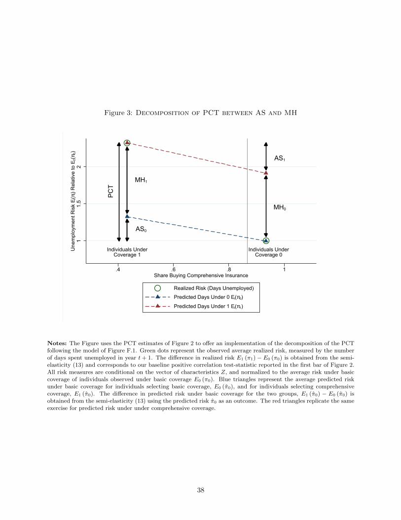
Figure 3: Decomposition of PCT between AS and MH

Individuals UnderCoverage 1

Individuals UnderCoverage 0

AS1

MH1

MH0

AS0

PCT

11.

52

Une

mpl

oym

ent R

isk

Ε i(π

i) R

elat

ive

to Ε

0(π0)

.4 .6 .8 1Share Buying Comprehensive Insurance

Realized Risk (Days Unemployed)Predicted Days Under 0 Εi(π0)

Predicted Days Under 1 Εi(π1)

Notes: The Figure uses the PCT estimates of Figure 2 to offer an implementation of the decomposition of the PCTfollowing the model of Figure F.1. Green dots represent the observed average realized risk, measured by the numberof days spent unemployed in year t + 1. The difference in realized risk E1 (π1) − E0 (π0) is obtained from the semi-elasticity (13) and corresponds to our baseline positive correlation test-statistic reported in the first bar of Figure 2.All risk measures are conditional on the vector of characteristics Z, and normalized to the average risk under basiccoverage of individuals observed under basic coverage E0 (π0). Blue triangles represent the average predicted riskunder basic coverage for individuals selecting basic coverage, E0 (π0), and for individuals selecting comprehensivecoverage, E1 (π0). The difference in predicted risk under basic coverage for the two groups, E1 (π0) − E0 (π0) isobtained from the semi-elasticity (13) using the predicted risk π0 as an outcome. The red triangles replicate the sameexercise for predicted risk under under comprehensive coverage.

38

Figure 4: Price Variation: Evolution of Premia p and of the Fraction of WorkersBuying the Comprehensive Coverage Around the 2007 Reform

100

150

200

250

300

350

Mon

thly

UI F

und

Prem

ium

(SEK

)(fo

r Em

ploy

ed U

nion

ized

Wor

kers

)

.76

.78

.8.8

2.8

4.8

6Fr

actio

n Bu

ying

Com

preh

ensi

ve C

over

age

2002 2003 2004 2005 2006 2007 2008 2009

Share members UI premium

Notes: The Figure reports the evolution of monthly premium for the supplemental UI coverage over time. Asexplained in Section 2.1, there are no sources of premium differentiation up to 2008, apart from small rebates forunion members and for unemployed individuals. Here, we report the value of the premium for employed unionmembers. The Figure shows a large and sudden increase in the premia paid for the supplemental coverage in 2007.This increase followed the surprise ousting of the Social Democrats from government after the September 2006 generalelection. Note that from July 2008 on, premia started to be differentiated across UI funds. For 2008 and 2009 wetherefore report the average monthly premium among unemployed union members across all UI funds. The Figurealso shows the evolution of the take-up of the comprehensive UI coverage, measured as the sum of all individualsbuying the comprehensive coverage divided by the total number of individuals aged 25 to 55 meeting the eligibilitycriteria for receiving UI benefits.

39

Figure 5: Price Variation: Unemployment Risk by Willingness-To-Pay

0

1

2

3

4

5

6

7D

ays

Spen

t Une

mpl

oyed

in 2

008

Group 1Under Comprehensive

in 2006 & 2007

MarginalsUnder Comprehensive

in 2006 only

Group 0Under Basic

in 2006 & 2007

A. Total Unemployment Duration in 2008

0

1

2

3

4

5

6

7

Day

s Sp

ent U

nem

ploy

ed in

200

8

Group 1Under Comprehensive

in 2006 & 2007

MarginalsUnder Comprehensive

in 2006 only

Group 0Under Basic

in 2006 & 2007

B. Predicted Risk Under Basic

0

1

2

3

4

5

6

7

Day

s Sp

ent U

nem

ploy

ed in

200

8

Group 1Under Comprehensive

in 2006 & 2007

MarginalsUnder Comprehensive

in 2006 only

Group 0Under Basic

in 2006 & 2007

C. Predicted Risk Under Comprehensive

Notes: The Figure reports average risk for three groups of individuals defined by descending order of willingness-to-pay. Group 1 individuals are in the comprehensive coverage both in 2006 and 2007: they have the highest valuationof the supplemental coverage (u > 0). Marginals M(p) were buying the comprehensive coverage in 2006 but switchout in 2007 when premia p increase: they are close to indifferent between the two coverages at current prices (u ≈ 0).Individuals from group 0 were neither buying the comprehensive coverage in 2006 nor in 2007, and have the lowestwillingness-to-pay for the supplemental coverage (u < 0). For each panel, we report E(π|Z = Z0, D = j), theaverage risk outcome π of each group j = 1,M, 0 estimated at the average value of Z for group 0. The vector Z arecharacteristics affecting contract differentiation. Panel A reports the average number of days spent unemployed in2008 for each group. Panel B plots the average predicted risk under basic coverage, and panel C the average predictedrisk under comprehensive coverage. See text for details.

Figure 6: Price Variation: Test of Residual Private Information

0.5

11.

52

2.5

33.

5Se

mi-E

last

icity

of R

isk

Mea

sure

w.r.

t Ins

uran

ce C

hoic

e

Baseline Baseline +Demog. Controls

Baseline +Pred. Risk

under Basic

Notes: The Figure uses the 2007 price reform to estimate how much adverse selection is left when controlling forobservable characteristics. The graph first reports the baseline semi-elasticity SemiBaselineM(p) of realized risk for themarginals M relative to the individuals always in the basic coverage. The second bar shows the same semi-elasticitywhere we include in specification (16) a set of dummies for age, gender, marital status, education (four categories),industry (1-digit code) and wealth level (quartiles). Interestingly, the semi-elasticity increases compared to ourbaseline when including these controls. This suggests these characteristics provide advantageous selection on average,such that if contracts were differentiated along these observable dimensions, adverse selection into comprehensivecoverage would actually be more severe. The third bar reports the semi-elasticity SemiResidualM(p) where we condition onpredictable risk by including in specification (16) twenty dummies for the predicted unemployment risk score underbasic coverage in both the inflated and count part of the model. Results indicate that there is no significant residualcorrelation left between realized risk and willingness-to-pay when we control for predicted unemployment risk. Seetext for details.

Figure 7: Benefit Variation: Regression Kink Design Analysis of Demand Responsesand Risk Based Selection

A. Replacement Rate B. Fraction BuyingUnder Comprehensive Coverage Comprehensive Coverage

.55

.6

.65

.7

.75

.8

Bene

fits

as fr

actio

n of

wag

e

500 600 700 800 900 1000 1100 1200Daily wage (SEK)

Estimated Change in Slopeβ1*100 = -.016 (.001)

.78

.8

.82

.84

.86

Pr. o

f Buy

ing

Com

preh

ensi

ve U

I500 600 700 800 900 1000 1100 1200

Daily Wage (SEK)

C. Predicted Risk D. Predicted RiskUnder Basic Coverage Under Comprehensive Coverage

Estimated Change in Slopeβ1*100 = .204 (.144)

1.5

22.

53

3.5

4Pr

edic

ted

Day

s of

Une

mpl

oym

ent

500 600 700 800 900 1000 1100 1200Daily Wage (SEK)

Estimated Change in Slopeβ1*100 = .279 (.105)

88.

59

9.5

1010

.5Pr

edic

ted

Day

s of

Une

mpl

oym

ent

500 600 700 800 900 1000 1100 1200Daily Wage (SEK)

Notes: The Figure presents the regression kink design based on the kinked schedule of benefits b1 in the compre-hensive coverage. The sample consists of all individuals from our baseline sample who become unemployed in yeart ∈ [2003; 2007] and were employed in year t − 1. Panel A shows the relationship between the daily wage prior tounemployment and the replacement rate, defined as average daily benefit received during unemployment from theIAF data divided by the daily wage. The panel shows that the relationship exhibits a sharp kink at w = 850SEK,the level of the cap in b1. Panel B plots the average fraction of individuals who bought the comprehensive coveragein year t by bins of the daily wage in year t. The data is residualized on the vectors of characteristics Z whichaffect the contract space and on the vector X which includes age, gender, level of education, region, family type andindustry. We report on the graph the linear fit and the estimate β1 corresponding to specification (18) estimatedusing a bandwidth of 350SEK. Panels C and D produce RKD graphs similar to panel B, using as outcomes predictedrisk under basic coverage in year t and predicted risk under comprehensive coverage in year t respectively.

Figure 8: Welfare Analysis

A. Cost Curves for Comprehensive and Basic Plan

E j(c

1-c0)

E1(c1)

E1(c0)

E0(c1)

E0(c0)

Group 1 Marginals Group 0

01,

000

2,00

03,

000

Cov

erag

e C

osts

(in

SEK)

.3 .4 .5 .6 .7 .8 .9 1Share Buying Comprehensive Insurance

B. Demand vs. Cost of Supplemental Coverage

p - Ep(c1-c0)

Group 1 Marginals Group 0

01,

500

3,00

04,

500

Valu

e an

d C

osts

(in

SEK)

.3 .4 .5 .6 .7 .8 .9 1Share Buying Comprehensive Insurance

Notes: The figure shows the demand and cost curves underlying the welfare implementation in Section 6. Panel Aplots the cost curves for the comprehensive and basic plan. For the basic (comprehensive) cost curve, we convertthe predicted days spent unemployed under basic (comprehensive) coverage in Figure (5) into the expected cost ofproviding basic (comprehensive) coverage for individuals from group 1, marginals and individuals from group 0 definedusing the 2007 price change. Following Figure (F.2), we locate the estimated average costs for the three groups atthe midpoint of the ranges of the corresponding valuation quantiles and then use a piece-wise linear interpolation toconstruct the cost curves. Panel B compares the willingness-to-pay and cost c of providing supplemental coverage fordifferent workers ranked based on their valuation u. The black triangles correspond to the difference between the costof providing the comprehensive plan and the basic plan (plotted separately in Panel A) for each of the three groups.The supplemental cost curve is then constructed using a piece-wise linear interpolation. The linear demand curveis an extrapolation of the share of individuals taking up the comprehensive plan at the pre- and post-reform prices(grey circles). The vertical distance between the demand and cost curves in Panel B denotes the fiscal externalityper marginal worker FEASp = [p1 − p0]−

[EM(p) (π1) b1 − EM(p) (π0) b0

]for different prices p.

Table 1: Summary Statistics

Mean P10 P50 P90

I. Unemployment

Displacement probability 3.05% - - -Displacement probability (exc. quits) 2.85% - - -Unemployment probability 3.65% - - -Days unemployed (unconditional) 5.28 0 0 0Unemployment spell duration (days) (if > 0) 147.39 22 91 305Predicted days unemployed under Basic 3.57 2.14 2.72 4.02Predicted days unemployed under Comprehen-sive

5.83 3.63 4.77 7.17

Fraction receiving layoff notification .05 - - -Fraction switching firms .09 - - -

II. Union andUI Fund Membership

Union membership .75 - - -UI fund membership (D) .86 - - -Fraction switching from coverage 0 to 1 .02 - - -Fraction switching from coverage 1 to 0 .01 - - -

III. Demographics

Age 40.88 28 40 52Years of education 12.86 11 12 16Fraction men .52 - - -Fraction married .44 - - -

IV. Income and WealthSEK 2003(K)

Gross earnings 249 100.3 231.2 388.8Net wealth 385.9 -160.8 90.9 1127.7Bank holdings 49.3 0 0 122.1

N 17,761,796

Notes: The Table provides summary statistics for our baseline sample over the period 2002 to 2006. The samplecomprises individuals who are between 18 and 60 years of age and have been working for at least 6 months. Itcontains 17.8 million worker × year observations. Unemployment is defined as a spell of non-employment, followingan involuntary job loss, and during which an individual has zero earnings, receives unemployment benefits andreports searching for a full time job. We define displacement as an involuntary job loss, due to a layoff or a quitfollowing a ‘valid reason’. Voluntary quits are not included in our measures of displacement and unemployment. Theprobability of displacement is the probability to be displaced in year t + 1 conditional on working in year t. Theunemployment probability is the probability to be unemployed in year t+ 1 unconditional on employment status inyear t. The fraction of workers receiving layoff notification comes from the layoff-notification register (VARSEL) andis defined as the fraction of workers that are employed in an establishment emitting a layoff notification in year t.The employer-employee matched data (RAMS) registers all existing labor contracts on a monthly basis. We definea “firm switch” as moving from having a labor contract with firm j to having a contract with firm k, without anyrecorded non-employment spell between these two contracts. UI fund membership information comes from tax datafor the period 2002 to 2006, during which premia were eligible for a 40% tax credit. The dummy variable D forbuying the comprehensive coverage in year t is defined as reporting any positive amount of premia paid in year t. Allearnings, income and asset level measures are from wealth and income registers, and are yearly measures in constantk2003SEK. All assets are aggregated at the household level and estimated at their market value. 1SEK2003 ≈ 0.11USD2003

Appendix A Observable Risk & Predicted Risk Model:

Further Material

In this appendix:

(i) we present the relationship in the Swedish labor market, between a series of observable risk

shifters, that are credibly exogenous to individuals’ own actions, and individuals’ unemploy-

ment risk.

(ii) we then present a model of predicted unemployment risk that combines all risk shifters to-

gether.

A.1 Observable Risk Shifters in the Swedish Labor Market

The institutional context and the richness of the Swedish registry data allows us to observe deter-

minants of unemployment risks that are arguably beyond the control of individuals. We present

here three such observable sources of risk variation and show how they correlate with individuals’

realized unemployment risk.

Average Firm Layoff Rates The first observable source of variation in unemployment risk

stems from firm level risk. Firm level risk can vary cross-sectionally, due to permanent differences

in turnover across firms, or over time, due to firms experiencing temporary shocks. We focus,

to start with, on the permanent component of firm level risk, and explore how this permanent

component correlates with an individual’s displacement probability.

For each individual i working in firm j, we define average firm displacement risk π−i,j as the

average probability of displacement of all other workers within the firm excluding individual i over

all years where the firm is observed active between 1990 and 2015.46 We then plot, in Figure A.1

panel A, our measure of average firm risk π−i,j in 20 bins of equal population size, against πi,j ,

the individual probability of displacement in t + 1, for all individuals ever employed during the

period 2002-2007. The figure shows first that there is significant heterogeneity in firms’ average

separation rates. Second, the figure provides clear evidence that individuals’ unemployment risk is

very strongly correlated with average firm level risk.

Layoff Notifications The second observable source of variation in unemployment risk stems

from variation in firm level risk over time. We leverage the fact that under Sweden’s employment-

46For this purpose we match the employer-employee registry (RAMS) from 1985 to 2015 with the Public Employ-ment Service (PES) registry for all years 1990-2015.

45

protection law, firms subject to a shock and intending to displace 5 or more workers simultaneously

must notify the Public Employment Service in advance. Once a notification is emitted, employers

need to come up with the list and dates for the intended layoffs. These layoffs may happen up

to 2 years after the original notification has been sent. The layoff notifications provide a source

of observable variation in firm displacement risk. In Figure A.2 we report the evolution of the

displacement probability of workers around the first layoff notification event in the history of the

firm. We define event year n as the year to/since the firm emits its first layoff notification and follow

an event study approach around that event. Our sample is the panel of workers who are employed

in the firm at the date this layoff notification is emitted to the PES. The graph shows that a layoff

notification is indeed associated with a sudden and large increase in the displacement probability

of workers. Immediately following the layoff notification, the displacement rate of workers jumps

by 6 percentage points compared to pre-notification levels, and remains high for about two years,

before decreasing and converging back to pre-notification levels.

Because the panel of workers is selected based on being employed in the firm in year n = 0, one

may worry that this surge in displacement rates is mechanical, as displacement can only increase

after year 0 conditional on all workers being employed in year 0. To mitigate this concern, we follow

a matching strategy and create a control panel of workers selected along the same procedure as the

original panel. We use nearest-neighbor matching to select a set of firms that are similar, along a

set of observable characteristics, to the firms emitting a layoff notification, but never emit a layoff

notification.47 We allocate to the matched firm in the control group a placebo event date equal to

the layoff notification date of her nearest-neighbor in the treated group of firms. We then select

workers that are in the control firm at the time of the placebo event date to create our matched

control panel. Results in Figure A.2 show that, pre-event, the displacement risk is very similar in

the control and treated groups, and that it evolves smoothly in the control firms around the event.

This evidence suggests that layoff notifications are a significant shifter of individuals’ unem-

ployment risk, as they immediately double the baseline displacement probability of workers.

Relative Tenure The third source of observable (and credibly exogenous) risk variation is at

the individual level and stems from the strict enforcement of the Last-In-First-Out (LIFO) prin-

ciple. When a firm wants to downsize within an establishment, the legal system prescribes that

displacement occurs by descending order of tenure within the establishment. In practice, workers

are divided into groups, defined by collective bargaining agreements in the establishment, and then

a tenure ranking within each group is constructed. The tenure ranking of an individual within her

establishment and collective bargaining agreement (CBA) group directly determines her probability

to be separated. A limitation of our data is that workers’ collective bargaining agreements are not

directly observed. Instead, we use detailed occupation codes as proxies for the CBAs, which is a

good approximation as most CBAs are done at the occupation level.

Figure A.1 panel B plots the probability of being displaced in t+ 1 among individuals working

47The covariates used for matching are the number of employees, the 4 digit sector codes of the firm, the averageearnings and average years of education of workers in the firm.

46

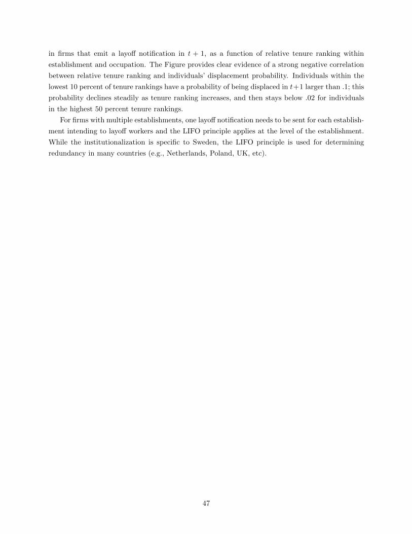
in firms that emit a layoff notification in t + 1, as a function of relative tenure ranking within

establishment and occupation. The Figure provides clear evidence of a strong negative correlation

between relative tenure ranking and individuals’ displacement probability. Individuals within the

lowest 10 percent of tenure rankings have a probability of being displaced in t+1 larger than .1; this

probability declines steadily as tenure ranking increases, and then stays below .02 for individuals

in the highest 50 percent tenure rankings.

For firms with multiple establishments, one layoff notification needs to be sent for each establish-

ment intending to layoff workers and the LIFO principle applies at the level of the establishment.

While the institutionalization is specific to Sweden, the LIFO principle is used for determining

redundancy in many countries (e.g., Netherlands, Poland, UK, etc).

47

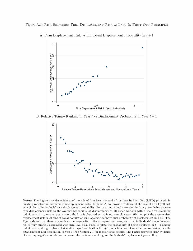
Figure A.1: Risk Shifters: Firm Displacement Risk & Last-In-First-Out Principle

A. Firm Displacement Risk vs Individual Displacement Probability in t+ 1

0.0

2.0

4.0

6.0

8.1

Indi

vidu

al D

ispl

acem

ent R

isk

in t+

1

0 .05 .1Firm Displacement Risk in t (exc. individual)

B. Relative Tenure Ranking in Year t vs Displacement Probability in Year t+ 1

0.0

5.1

.15

Dis

plac

emen

t Pro

babi

lity

in Y

ear t

+1

0 .2 .4 .6 .8 1Relative Tenure Rank Within Establishment and Occupation in Year t

Notes: The Figure provides evidence of the role of firm level risk and of the Last-In-First-Out (LIFO) principle increating variation in individuals’ unemployment risks. In panel A, we provide evidence of the role of firm layoff riskas a shifter of individuals’ own displacement probability. For each individual i working in firm j, we define averagefirm displacement risk as the average probability of displacement of all other workers within the firm excludingindividual i, π−i,j over all years where the firm is observed active in our sample years. We then plot the average firmdisplacement risk in 20 bins of equal population size, against the individual probability of displacement in t+ 1. TheFigure shows that there is significant heterogeneity in firms’ separation rates, and that individuals’ unemploymentrisk is very strongly correlated with firm level risk. Panel B plots the probability of being displaced in t + 1 amongindividuals working in firms that emit a layoff notification in t + 1, as a function of relative tenure ranking withinestablishment and occupation in year t. See Section 2.1 for institutional details. The Figure provides clear evidenceof a strong negative correlation between relative tenure ranking and individuals’ displacement probability.

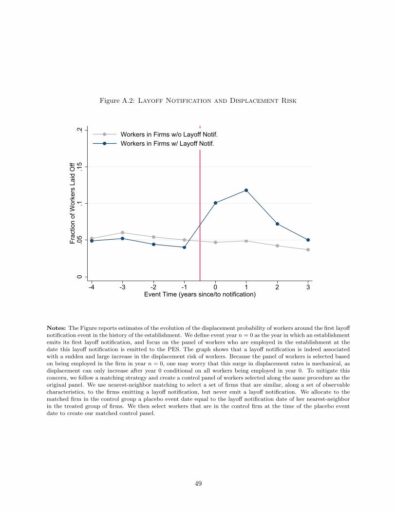
Figure A.2: Layoff Notification and Displacement Risk

0.0

5.1

.15

.2Fr

actio

n of

Wor

kers

Lai

d O

ff

-4 -3 -2 -1 0 1 2 3Event Time (years since/to notification)

Workers in Firms w/o Layoff Notif.Workers in Firms w/ Layoff Notif.

Notes: The Figure reports estimates of the evolution of the displacement probability of workers around the first layoffnotification event in the history of the establishment. We define event year n = 0 as the year in which an establishmentemits its first layoff notification, and focus on the panel of workers who are employed in the establishment at thedate this layoff notification is emitted to the PES. The graph shows that a layoff notification is indeed associatedwith a sudden and large increase in the displacement risk of workers. Because the panel of workers is selected basedon being employed in the firm in year n = 0, one may worry that this surge in displacement rates is mechanical, asdisplacement can only increase after year 0 conditional on all workers being employed in year 0. To mitigate thisconcern, we follow a matching strategy and create a control panel of workers selected along the same procedure as theoriginal panel. We use nearest-neighbor matching to select a set of firms that are similar, along a set of observablecharacteristics, to the firms emitting a layoff notification, but never emit a layoff notification. We allocate to thematched firm in the control group a placebo event date equal to the layoff notification date of her nearest-neighborin the treated group of firms. We then select workers that are in the control firm at the time of the placebo eventdate to create our matched control panel.

49

A.2 Predicting Risk Using Observable Risk Shifters: a Zero-Inflated-Poisson

Model of Unemployment Risk

We now present the model we use to compute the best predictor of future unemployment risk given

all currently observed individual characteristics. To do so, we leverage the rich set of observables

available in the Swedish registry data, and the various institutional features of the Swedish labor

market.

Setup The measure of unemployment risk π that we model is the number of days an individual

is expected of spending unemployed in t+ 1. This is the relevant measure of risk to the UI system

given insurance choices made in year t.48

The distribution of days spent unemployed is defined only over non-negative integers, and

exhibits a significant mass at zero. To account for these facts, we model π using a zero-inflated

Poisson model. The expected number of days unemployed conditional on a vector of characteristics

X therefore takes the following form:

E(π|X) = (1− f(0|XI)) exp(XC′βC)

For the zero-inflated part of the process, we parametrize the probability f(0) using a logit: f(0|XI) =

exp(XI′βI)/(1 + exp(XI′βI)). We will allow for the set of risk predictors XI and XC entering re-

spectively the inflated part and the count part, to differ.

To account for moral hazard, we allow the risk of individuals with similar characteristics X to

differ if they are observed under the basic coverage or under the comprehensive coverage. To this

purpose, we estimate separately two models of predicted risk. The first model is the predicted risk

given X under the basic coverage π0 = E(π0|X). This model is estimated on individuals who are

observed under the basic coverage in t. The second model is the predicted risk given X under the

comprehensive coverage π1 = E(π1|X), which we estimate on individuals who are observed under

the comprehensive coverage in t.

Lasso Penalization In terms of model selection, we discipline the choice of the many potential

regressors by using the adaptive Lasso procedure for a zero-inflated Poisson (ZIP) model proposed

by Banerjee et al. [2018]. The ZIP Log Likelihood function with LASSO penalty works in the

following way.

Let XC = {xC1 , ..., xCK} be the set of K regressors associated with predicting the number of

days unemployed, conditional on some unemployment, according to a Poisson distribution. The

corresponding coefficients are: {βC1 , ..., βCK}. Let XI = {xI1, ..., xIJ} be the set of J regressors associ-

ated with predicting some unemployment, according to a logistic distribution. The corresponding

48If an individual has bought the comprehensive coverage throughout year t, then the days she spends unemployedin year t+ 1 will be covered by the comprehensive benefits. In that sense, the relevant risk to determine the cost ofproviding the comprehensive coverage to an individual buying that coverage in year t is the expected number of daysshe will spend unemployed in year t+ 1.

50

coefficients are: {βI1 , ..., βIJ}. The number of days (integers) spent unemployed by individual i is

πi. Then we can write down the ZIP Log Likelihood function with LASSO penalty as follows:

L = L1 + L2 − L3 − PC − PI

Where each of the L1, L2, L3 components are defined as follows:

L1 =n∑

i:πi=0

log[exp(X ′Ii βI) + exp(− exp(X ′Ci β

C))]

L2 =n∑

i:πi>0

{πiX ′Ci βC + exp(−X ′Ci βC)− ln(πi!)}

L3 =

n∑i=1

log[1 + exp(X ′Ii βI)]

And the PC , PI components are defined as follows,

PC = λC

K∑k=1

|βCk |

PI = λI

J∑j=1

|βIj |

Estimation We can then estimate the model for various levels of penalization for the count part

λC and the inflated part of the model λI . In practice, we draw 50 pairs of λC and λI . The largest

pair is chosen so that all variables except the constant are set to zero. This corresponds to the

largest penalization.

We then randomly select a subset of observations from our sample to obtain a training sample,

the rest of the observation is considered our test sample. We estimate the model on the training

sample for all 50 pairs of λC and λI . We then compute the MSE on the test sample for all 50

models, and select the lambda pair associated with the smallest MSE on the test sample.

Predictors The regressors we allow to initially enter the model are individual log earnings, family

type, nine age bins, gender, twelve dummies for education level, year fixed effects, region fixed

effects, industry fixed effects, dummies for the past layoff history of the individual, dummies for

the layoff notification history of the firm, the leave-out mean of firm layoff risk, union membership,

tenure rank, interactions between tenure ranking and firm layoff risk and interactions between

tenure ranking and layoff notification history of the firm. We allow all these predictors to enter in

both the count and inflated part.

When varying the level of penalization in the model, starting from the highest penalization,

we can see what variables are the strongest predictors of the inflate and count part of unemploy-

51

ment risk. For the inflate component, the first variables to become significant are firm layoff risk,

layoff notification dummies, and relative rank. This confirms the important role played by the

institutional features of the Swedish labor market in determining unemployment risk. For the

count component, the first variables to become significant (by order) are those associated with age,

gender, education level, income, regions and years

The results show that the optimal penalization factors λ associated with the count component

are smaller while those associated with the zero component are higher, thus penalizing the inclusion

of variables in the latter more. As a result, in our preferred model of predicted risk, in the zero

component, a large share of variables have a coefficient set to zero.

Model fit As explained in section 2.3, we first assess the quality of the model fit in Figure 1 by

plotting bin scatters of the relationship between predicted risk under basic (resp. comprehensive)

coverage and actual realized risk for individuals under basic (resp. comprehensive) coverage. In

both panels, the relationship is close to the 45 degree line indicating that the model does a good

job at predicting the average realization of unemployment risk. In Table A.1 below, we provide

further summary statistics on the distribution of predicted risk according to our model. In Panel

A, we focus on individuals observed under the basic coverage, and compare the distribution of their

realized risk π0 to the distribution of their predicted risk under basic coverage π0. The average

risk predicted by the model (2.95) is very close to the average realized risk (2.83). In Panel B,

we do a similar exercise, focusing on individuals observed under the comprehensive coverage. We

compare the distribution of their realized risk π1 to the distribution of their predicted risk under

basic coverage π1. We find again that the average risk predicted by the model (5.90) is very close

to the average realized risk (5.65). In both panels, we find that there is much less dispersion in

predicted risk than in realized risk. The standard deviation of predicted risk is roughly six times

smaller than that of realized risk. This confirms that there still remains a significant dimension

of idiosyncratic unemployment risk beyond what can be predicted by even our very rich set of

observables.

52

Table A.1: Distribution of Realized and Predicted Risk for Individuals under Basic and underComprehensive Coverage

Panel A. Predictable Risk Under Basic

π0 π0

P25 0 2P50 0 3P75 0 3P90 0 4P99 107 13P99.9 346 32Mean 2.84 2.95s.d. 22.54 2.47

N 2,2296,727 2,232,136

Panel B. Predictable Risk Under Comprehensive

π1 π1

P25 0 4P50 0 5P75 0 6P90 0 7P99 184 30P99.9 365 80Mean 5.65 5.91s.d. 33.17 5.86

N 15,003,779 14,879,543

Notes: The table reports moments of the distribution of predicted risk and realized risk from our sample of workersfor years 2002 to 2006. Panel A focuses on individuals who are observed under the basic coverage in t. The firstcolumn reports moments of the distribution of their realized risk π0 while the second column reports moments of thedistribution of our measure of predicted risk under basic coverage π0. Panel B focuses on individuals who are observedunder the comprehensive coverage in t. The first column reports moments of the distribution of their realized risk π1

while the second column reports moments of the distribution of our measure of predicted risk under comprehensivecoverage π1.

53

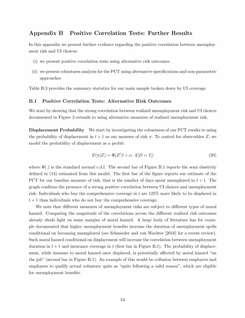
Appendix B Positive Correlation Tests: Further Results

In this appendix we present further evidence regarding the positive correlation between unemploy-

ment risk and UI choices:

(i) we present positive correlation tests using alternative risk outcomes.

(ii) we present robustness analysis for the PCT using alternative specifications and non-parametric

approaches

Table B.3 provides the summary statistics for our main sample broken down by UI coverage.

B.1 Positive Correlation Tests: Alternative Risk Outcomes

We start by showing that the strong correlation between realized unemployment risk and UI choices

documented in Figure 2 extends to using alternative measures of realized unemployment risk.

Displacement Probability We start by investigating the robustness of our PCT results to using

the probability of displacement in t+ 1 as our measure of risk π. To control for observables Z, we

model the probability of displacement as a probit:

E(π|Z) = Φ(Z ′β + α · 1[D = 1]) (20)

where Φ(.) is the standard normal c.d.f. The second bar of Figure B.1 reports the semi elasticity

defined in (13) estimated from this model. The first bar of the figure reports our estimate of the

PCT for our baseline measure of risk, that is the number of days spent unemployed in t+ 1. The

graph confirms the presence of a strong positive correlation between UI choices and unemployment

risk: Individuals who buy the comprehensive coverage in t are 125% more likely to be displaced in

t+ 1 than individuals who do not buy the comprehensive coverage.

We note that different measures of unemployment risks are subject to different types of moral

hazard. Comparing the magnitude of the correlations across the different realized risk outcomes

already sheds light on some margins of moral hazard. A large body of literature has for exam-

ple documented that higher unemployment benefits increase the duration of unemployment spells

conditional on becoming unemployed (see Schmieder and von Wachter [2016] for a recent review).

Such moral hazard conditional on displacement will increase the correlation between unemployment

duration in t+ 1 and insurance coverage in t (first bar in Figure B.1). The probability of displace-

ment, while immune to moral hazard once displaced, is potentially affected by moral hazard “on

the job” (second bar in Figure B.1). An example of this would be collusion between employers and

employees to qualify actual voluntary quits as “quits following a valid reason”, which are eligible

for unemployment benefits.

54

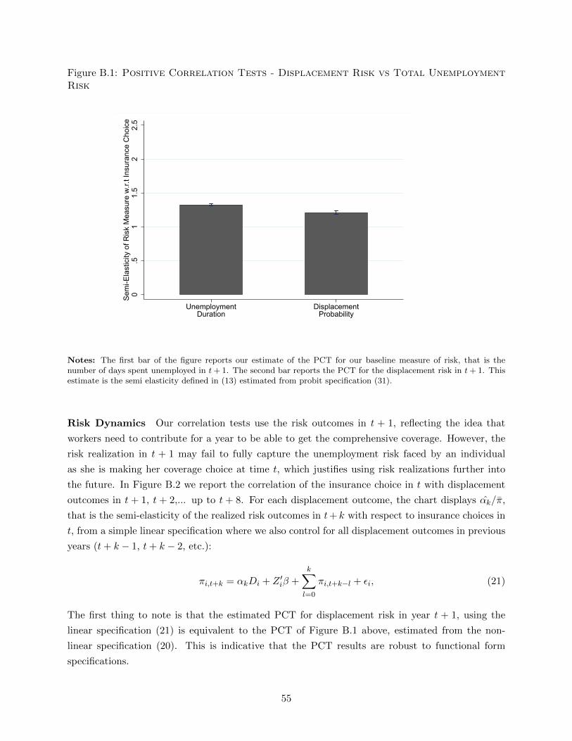
Figure B.1: Positive Correlation Tests - Displacement Risk vs Total UnemploymentRisk

0.5

11.

52

2.5

Sem

i-Ela

stic

ity o

f Ris

k M

easu

re w

.r.t I

nsur

ance

Cho

ice

UnemploymentDuration

DisplacementProbability

Notes: The first bar of the figure reports our estimate of the PCT for our baseline measure of risk, that is thenumber of days spent unemployed in t+ 1. The second bar reports the PCT for the displacement risk in t+ 1. Thisestimate is the semi elasticity defined in (13) estimated from probit specification (31).

Risk Dynamics Our correlation tests use the risk outcomes in t + 1, reflecting the idea that

workers need to contribute for a year to be able to get the comprehensive coverage. However, the

risk realization in t + 1 may fail to fully capture the unemployment risk faced by an individual

as she is making her coverage choice at time t, which justifies using risk realizations further into

the future. In Figure B.2 we report the correlation of the insurance choice in t with displacement

outcomes in t + 1, t + 2,... up to t + 8. For each displacement outcome, the chart displays αk/π,

that is the semi-elasticity of the realized risk outcomes in t+ k with respect to insurance choices in

t, from a simple linear specification where we also control for all displacement outcomes in previous

years (t+ k − 1, t+ k − 2, etc.):

πi,t+k = αkDi + Z ′iβ +k∑l=0

πi,t+k−l + εi, (21)

The first thing to note is that the estimated PCT for displacement risk in year t + 1, using the

linear specification (21) is equivalent to the PCT of Figure B.1 above, estimated from the non-

linear specification (20). This is indicative that the PCT results are robust to functional form

specifications.

55

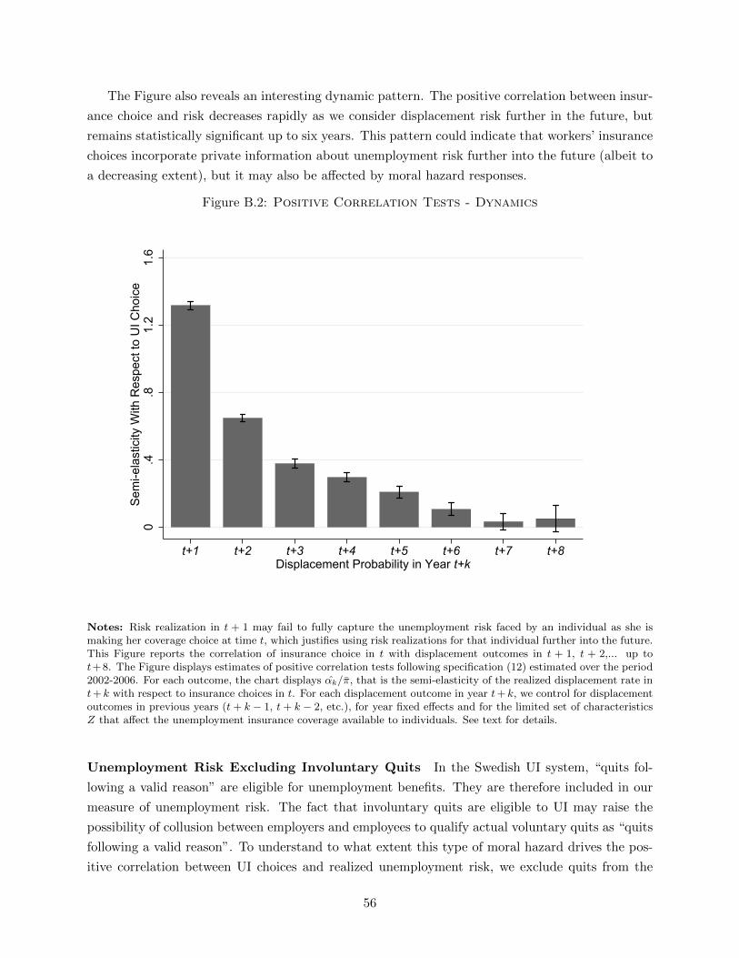
The Figure also reveals an interesting dynamic pattern. The positive correlation between insur-

ance choice and risk decreases rapidly as we consider displacement risk further in the future, but

remains statistically significant up to six years. This pattern could indicate that workers’ insurance

choices incorporate private information about unemployment risk further into the future (albeit to

a decreasing extent), but it may also be affected by moral hazard responses.

Figure B.2: Positive Correlation Tests - Dynamics

0.4

.81.

21.

6Se

mi-e

last

icity

With

Res

pect

to U

I Cho

ice

t+1 t+2 t+3 t+4 t+5 t+6 t+7 t+8Displacement Probability in Year t+k

Notes: Risk realization in t + 1 may fail to fully capture the unemployment risk faced by an individual as she ismaking her coverage choice at time t, which justifies using risk realizations for that individual further into the future.This Figure reports the correlation of insurance choice in t with displacement outcomes in t + 1, t + 2,... up tot+8. The Figure displays estimates of positive correlation tests following specification (12) estimated over the period2002-2006. For each outcome, the chart displays αk/π, that is the semi-elasticity of the realized displacement rate int+ k with respect to insurance choices in t. For each displacement outcome in year t+ k, we control for displacementoutcomes in previous years (t+ k − 1, t+ k − 2, etc.), for year fixed effects and for the limited set of characteristicsZ that affect the unemployment insurance coverage available to individuals. See text for details.

Unemployment Risk Excluding Involuntary Quits In the Swedish UI system, “quits fol-

lowing a valid reason” are eligible for unemployment benefits. They are therefore included in our

measure of unemployment risk. The fact that involuntary quits are eligible to UI may raise the

possibility of collusion between employers and employees to qualify actual voluntary quits as “quits

following a valid reason”. To understand to what extent this type of moral hazard drives the pos-

itive correlation between UI choices and realized unemployment risk, we exclude quits from the

56

definition of unemployment. To do this, we use the fact that in the IAF data, a variable indicates

whether an unemployment spell starts following a “quit for a valid reason”.

We use again a simple linear specification:

πi = αDi + Z ′iβ + εi, (22)

In Figure B.3, we report α/π, that is the semi-elasticity of the realized risk outcome in t+ 1 with

respect to the insurance choice in t from this specification. We first use as an outcome π the total

number of days spent unemployed in t + 1, when including quits (first bar). Then, in the second

bar, we report results where we use as an outcome π the total duration spent unemployed in t+ 1

when excluding involuntary quits from the definition of unemployment risk. We then replicate this

exercize using as an outcome the probability of displacement in t + 1 when including quits (third

bar) and when excluding involuntary quits (fourth bar) from the definition of displacement risk.

The figure shows that the positive correlation between unemployment risk and UI choices is almost

unaffected by the inclusion or exclusion of involuntary quits.

57

Figure B.3: Positive Correlation Tests: Risk Outcomes Including and ExcludingInvoluntary Quits

0.5

11.

52

Sem

i-Ela

stic

ity o

f Ris

k M

easu

re w

.r.t I

nsur

ance

Cho

ice

UnemploymentDuration

UnemploymentDuration

Excl. Quits

DisplacementProbability

DisplacementProbabilityExcl. Quits

Notes: This Figure reports the correlation of insurance choice in t with risk outcomes in t+ 1. The Figure displaysestimates of positive correlation tests following specification (22) estimated over the period 2002-2006. For eachoutcome, the chart displays α/π, that is the semi-elasticity of the realized risk with respect to insurance choices int. For each outcome, we control for year fixed effects and for the limited set of characteristics Z that affect theunemployment insurance coverage available to individuals. See text for details.

58

B.2 Bivariate Probit & Non-parametric Tests

We now further investigate functional form restrictions and provide correct inference for the corre-

lation tests.

First, we provide results of bivariate probit tests, popularized by Chiappori and Salanie [2000].

We specify both the choice of insurance coverage and the realization of our binary measure of

unemployment risk (i.e., the probability of displacement) as probit models:

ui = 1[Z ′α1 + ε > 0]

πi = 1[Z ′α2 + η > 0](23)

where ui = ui,1 − ui,0 is the short-hand notation for the difference in indirect expected utility

for individual i between being in the comprehensive plan and being in the basic plan. We allow

for correlation ρ between the two error terms ε and η. The vector of controls Z contains the same

variables as in specification (12). We provide in Table B.1 estimates of ρ and formal tests of the null

that ρ = 0. Results confirm the presence of a strong and significant correlation between insurance

choices and realized unemployment risk.

The functional forms involved in the bivariate probit tests are still restricted to the latent models

being linear and the errors normal, excluding cross-effects or more complicated non-linear functions

of the variables in Z. We therefore also produce results from non-parametric tests as in Chiappori

and Salanie [2000]. The procedure of the test consists in partitioning the data into cells where

all observations in a given cell have the same value for the variables in Z. The procedure then

computes within each cell a Pearson’s χ2 test statistic for independence between u and π. This

test statistic is asymptotically distributed as a χ2(1) under the null hypothesis that u and π are

statistically independent (within the cell). We report in the first column of Table B.2 results from

this non-parametric procedure when cells are defined using the same controls Z as in specification

(12) and where our risk measure π is the probability of displacement. Results again strongly confirm

the presence of a positive correlation between insurance choices and unemployment probability. In

Figure B.4 panel 1, we display the empirical distribution of the Pearson’s χ2 test statistics computed

from all the cells to allow for comparison with a theoretical χ2(1) distribution. Taking the largest

absolute difference between the theoretical and the empirical distribution gives the Kolmogorov-

Smirnov test statistic reported in Table B.2.

In columns (2) to (4) of Table B.2, we explore the robustness of the positive correlation test

to adding more observable characteristics in the vector Z. In other words, we want to explore

how much positive correlation would remain if the UI policy was allowed to differentiate coverage

or prices along obvious observable dimensions that do not currently enter the UI policy schedule

(such as age, gender, etc.). To this effect, we reproduce the non-parametric Kolmogorov-Smirnov

test adding sequentially more observable characteristics to the vector Z when partitioning the

data into cells. We start in column (2) of Table B.2 by adding demographic controls : age, then

gender, and marital status. The Kolmogorov-Smirnov test statistic increases sharply, indicating

that demographics may offer advantageous selection. Yet, we can still strongly reject the null

59

Table B.1: Positive Correlation Tests: Bivariate Probits

Test ρ = 0

ρ s.d. χ2 P-Value

Proba. of displacement .3047 .0030 8842.4 0.00

Proba. of displacement excl. quits .3056 .0031 8493.9 0.00

Notes: The Table reports positive correlation estimates between insurance and risk using bivariate probit models.We specify both the choice of insurance coverage and the probability of displacement as probit models allowing forcorrelation ρ between the two error terms ε and η. The Table reports estimates of ρ and its standard error. We alsoreport results of formal tests of the null that ρ = 0. In the first row, we consider the probability of displacement. Inthe second row we consider the probability of displacement excluding quits, as some quits may be eligible for UIafter a waiting period. See text for details.

of no positive correlation between risk and insurance choice. In column (3), we add controls for

education (four categories), and industry (1-digit code). The Kolmogorov-Smirnov test statistic

does not seem to be affected much by the inclusion of these controls for skills and other labor

market characteristics. In column (4), we finally add controls for past unemployment history

(dummies for having been unemployed in t− 1, t− 2 and up to t− 8). The Kolmogorov-Smirnov

test statistic decreases as a result, suggesting that past unemployment history creates significant

adverse selection.

For all specifications of columns (1) to (4) of Table B.2, the corresponding panels 1 to 4 of

Figure B.4 display the empirical distribution of the Pearson’s χ2 test statistics computed from all

the cells to allow for comparison with a theoretical χ2(1) distribution.

60

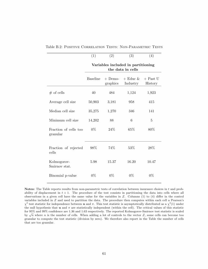
Table B.2: Positive Correlation Tests: Non-Parametric Tests

(1) (2) (3) (4)

Variables included in partitioningthe data in cells

Baseline + Demo- + Educ & + Past Ugraphics Industry History

# of cells 40 484 1,124 1,923

Average cell size 50,903 3,181 958 415

Median cell size 35,275 1,270 346 141

Minimum cell size 14,202 88 6 5

Fraction of cells toogranular

0% 24% 65% 80%

Fraction of rejectedcells

98% 74% 53% 28%

Kolmogorov-Smirnov stat.

5.98 15.37 16.20 10.47

Binomial p-value 0% 0% 0% 0%

Notes: The Table reports results from non-parametric tests of correlation between insurance choices in t and prob-ability of displacement in t + 1. The procedure of the test consists in partitioning the data into cells where allobservations in a given cell have the same value for the variables in Z. Columns (1) to (4) differ in the controlvariables included in Z and used to partition the data. The procedure then computes within each cell a Pearson’sχ2 test statistic for independence between u and π. This test statistic is asymptotically distributed as a χ2(1) underthe null hypothesis that u and π are statistically independent (within the cell). The critical values of this statisticfor 95% and 99% confidence are 1.36 and 1.63 respectively. The reported Kolmogorov-Smirnov test statistic is scaledby√n where n is the number of cells. When adding a lot of controls to the vector Z, some cells can become too

granular to compute the test statistic (division by zero). We therefore also report in the Table the number of cellsthat are too granular.

61

Figure B.4: Positive Correlation Tests - Distribution of χ2 test statistics from allcells vs Theoretical χ2(1) distribution - Additional Controls

1. Baseline 2. + Demographics

0.2

.4.6

.81

0 200 400 600T Statistic

Empirical DistributionTheoretical Distribution 0

.2.4

.6.8

1

0 100 200 300 400 500T Statistic

Empirical DistributionTheoretical Distribution

3. + Educ/Industry 4. + Past U History

0.2

.4.6

.81

0 50 100 150 200 250T Statistic

Empirical DistributionTheoretical Distribution 0

.2.4

.6.8

1

0 50 100 150 200T Statistic

Empirical DistributionTheoretical Distribution

Notes: The Figure displays the empirical distribution of the Pearson’s χ2 test statistics for independence betweenu (UI choices) and π, the probability of layoff in t + 1, computed from all the cells where we split individuals incells corresponding to various observable characteristics. In panel 1, we only use priced characteristics (baselinecontrols of the positive correlation tests), corresponding to the test implemented in column (1) of Table B.2. Inpanel 2, we add controls for demographics (cf. column (2) of Table B.2). Panel 3 and 4 add education, industry andpast unemployment history controls (cf. column (3) and (4) of Table B.2). The χ2 test statistic is asymptoticallydistributed as a χ2(1) under the null hypothesis that u and π are statistically independent (within the cell). Wetherefore compare this distribution with a theoretical χ2(1) distribution. Taking the largest absolute differencebetween the theoretical and the empirical distribution gives the Kolmogorov-Smirnov test statistic reported in TableB.2.

Table B.3: Summary Statistics - By Coverage

A. Under Basic B. Under Comprehensive

Mean P10 P50 P90 Mean P10 P50 P90

I. Unemployment

Displacement probability 1.96% - - - 3.21% - - -Displacement probability (exc. quits) 1.81% - - - 3% - - -Unemployment probability 2.29% - - - 3.85% - - -Days unemployed 2.84 0 0 0 5.65 0 0 0Predicted days unemployed under Basic 2.96 1.89 2.58 3.68 3.66 2.18 2.74 4.09Predicted days unemployed under Compre-hensive

5.34 3.45 4.67 6.82 5.91 3.66 4.78 7.24

Unemployment spell duration (days) 137.57 26 90 283 148.26 22 91 307Fraction receiving layoff notification .04 - - - .06 - - -Fraction switching firms .1 - - - .09 - - -

II. Union and UI Fund Membership

Union membership .13 - - - .84 - - -Switch from coverage 0 to 1 - - - - .02 - - -Switch from coverage 1 to 0 .01 - - - - - - -

III. Demographics

Age 35.52 25 33 55 41.7 27 42 55Years of education 12.97 11 12 16 12.84 11 12 16Fraction men .63 - - - .51 - - -Fraction married .32 - - - .46 - - -

IV. Income and Wealth, SEK 2003(K)

Gross earnings 233.8 65.3 186.7 416 251.5 115 234.9 385.4Net wealth 649.6 -195.1 25.7 1521.7 343.5 -155.5 102.4 1083.5Bank holdings 73.9 0 0 135.8 45.3 0 0 120.4

N 2,296,727 15,003,779

Notes: The Table breaks down the summary statistics by UI coverage for our main sample of interest over the period2002 to 2006. See Table 1.

63

Appendix C Impact of Predictable Risk on UI Choice: Further

Evidence

In this appendix we present further evidence regarding the relationship between predictable risk

and UI choices:

(i) we present non-parametric evidence of the relationship linking UI choices to both π0 and π1

(ii) we present quasi-experimental evidence showing how the various institutional risk shifters

detailed in Appendix A, which enter our predicted risk model, separately affect selection into

coverage.

C.1 Non-Parametric Evidence on the Relationship between Predicted Risk and

Insurance Choice

The positive correlation tests between predicted risk and UI choice from section 4.2 shows clearly

that individuals buying the supplemental coverage have a higher predictable risk on average in

both the basic coverage (E1[π0] > E0[π0]) and the comprehensive coverage (E1[π1] > E0[π1]). We

provide here more detailed non-parametric evidence on the relationship between insurance choice

and predicted risk in both coverages.

For this purpose, Figure C.1 offers a bin scatter correlating the probability to buy the com-

prehensive UI coverage in year t with the predicted number of days unemployed of individual i,

respectively under the basic coverage π0 and under the comprehensive coverage π1, based on her

observable characteristics year t. The graph confirms evidence from the positive correlation tests

of a strong positive correlation between individuals’ predictable risk and their probability to buy

the comprehensive UI coverage. Interestingly, the graph also suggests that the strong positive cor-

relation between risk and insurance coverage is mostly driven by what happens at the bottom of

the predicted risk distribution. Only about a half of individuals at the bottom of the predicted risk

distribution (π1 < 2 days) buy the comprehensive coverage. But this fraction quickly rises as the

predicted risk increases. It is then very stable, at around 85 to 90% for individuals with predicted

risk π1 < 5 days. Note finally that conditional on the fraction buying the comprehensive coverage,

the difference between predicted risk under basic and under comprehensive coverage captures the

presence of moral hazard.

C.2 Risk Shifter & UI Choices I: Average Firm Layoff Risk

The previous evidence focuses on risk measures from our predicted risk model. This model folds

all sources of variations of observable risk together into a unique measure of predictable risk. We

now also shed light on how the various institutional risk shifters that enter the predicted risk model

individually affect selection into coverage.

The first source of risk variation is average firm level risk. We define again the average firm

displacement risk π−i,j of worker i working in firm j as the average probability of displacement

64

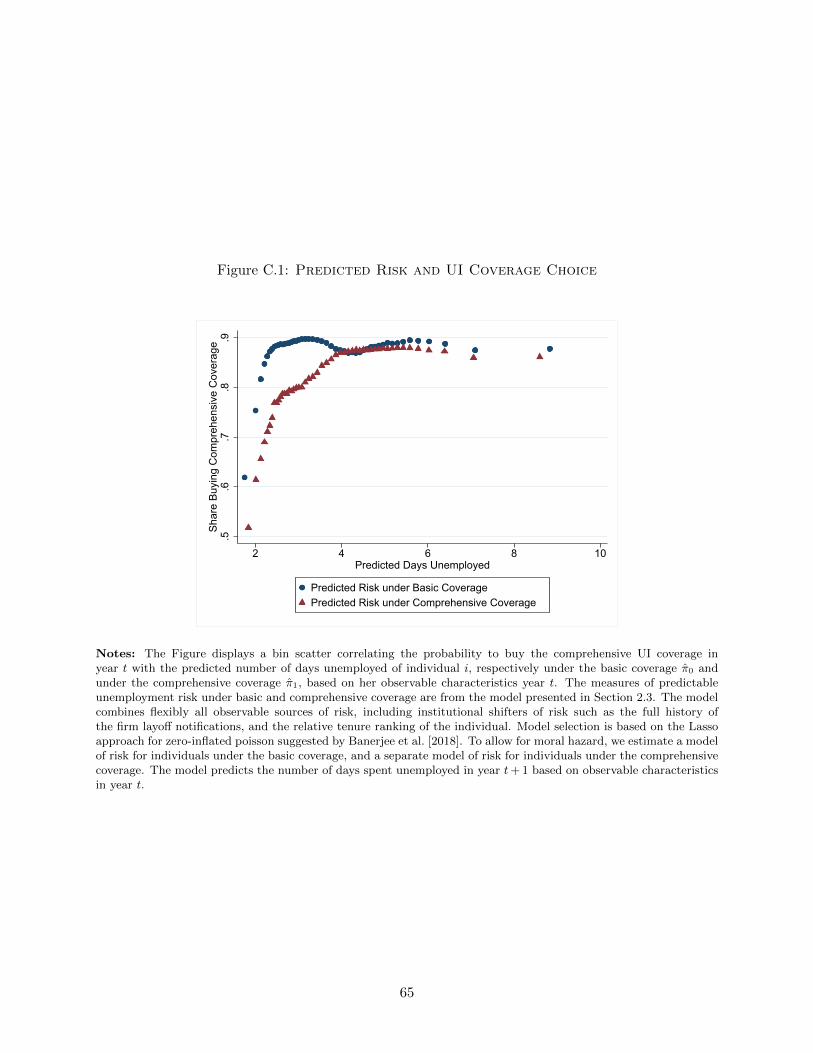
Figure C.1: Predicted Risk and UI Coverage Choice

.5.6

.7.8

.9Sh

are

Buyi

ng C

ompr

ehen

sive

Cov

erag

e

2 4 6 8 10Predicted Days Unemployed

Predicted Risk under Basic CoveragePredicted Risk under Comprehensive Coverage

Notes: The Figure displays a bin scatter correlating the probability to buy the comprehensive UI coverage inyear t with the predicted number of days unemployed of individual i, respectively under the basic coverage π0 andunder the comprehensive coverage π1, based on her observable characteristics year t. The measures of predictableunemployment risk under basic and comprehensive coverage are from the model presented in Section 2.3. The modelcombines flexibly all observable sources of risk, including institutional shifters of risk such as the full history ofthe firm layoff notifications, and the relative tenure ranking of the individual. Model selection is based on the Lassoapproach for zero-inflated poisson suggested by Banerjee et al. [2018]. To allow for moral hazard, we estimate a modelof risk for individuals under the basic coverage, and a separate model of risk for individuals under the comprehensivecoverage. The model predicts the number of days spent unemployed in year t+ 1 based on observable characteristicsin year t.

65

of all other workers within firm j excluding individual i over all years where the firm is observed

active in our sample years.

In section Appendix A we showed that there is significant heterogeneity in these average firms’

separation rates, and that individuals’ unemployment risk is very strongly correlated with this

average firm level risk (panel A of Figure A.1).

We now investigate how average firm level risk correlates with unemployment insurance choices.

Cross-Sectional Evidence The first strategy consists in simply using the cross-sectional varia-

tion in displacement risk across firms. In Figure C.2 panel A, we group individuals in 50 equal size

bins of firm layoff risk, and plot their average firm layoff risk against their average probability of

buying supplemental coverage, residualized on the same vector Z of baseline controls affecting UI

contracts used in the positive correlation test of Section 4.1.

The graph displays a strong positive correlation between firm layoff risk and individuals’ prob-

ability to buy the comprehensive UI coverage

We then estimate the correlation between average firm level risk π−i,j and willingness-to-pay

by running the following two-stage least square specification:

Di = β2SLS · πi + Z ′iα1 + ε

πi = ζ · π−i,j + Z ′iα2 + η(24)

where Di is our indicator variable for buying the supplemental coverage. This specification instru-

ments individual realized risk by the average firm layoff risk and therefore exploits only variation

in predictable risk coming from average firm layoff risk. For useful comparison, we also report the

coefficient estimate βOLS of the following OLS specification correlating D with individual risk:

Di = βOLS · πi + Z ′iα+ ν (25)

We estimate both models on our baseline sample of workers pooling all observations for years

2002 to 2006. We use as a measure of realized risk πi the realized displacement risk excluding quits

in year t + 1. We find a positive and strongly significant coefficient β2SLS = .50 (.01) indicating

that workers who work in firms that exhibit higher turnover rates are significantly more likely to

buy the comprehensive coverage.

We also find that β2SLS is much larger than βOLS , which is also informative. Clearly, the two-

stage least square procedure removes potential attenuation bias from measurement error in βOLS .

But the two-stage least square, by projecting choices only on the average firm layoff dimension

of displacement risk introduces some potential selection, if Cov(π−i,j , ε) 6= 0. In other words, if

workers who self-select into riskier firms are different along observed or unobserved characteristics

correlated with willingness-to-pay for insurance, β2SLS will capture this additional selection effect.

In panel B of Figure C.2, we explore the importance of such selection along observable charac-

teristics in explaining the magnitude of β2SLS . We introduce in the vector Z of specifications (24)

and (25) a rich set of additional controls: age, gender, marital status, education (four categories),

66

industry (1-digit code), occupation (1-digit code), wealth level (quartiles) and past unemployment

history (dummies for having been unemployed in t−1, t−2 and up to t−8). We still find a strong

positive correlation between insurance choices and firm layoff risk (β2SLS = .245). But adding these

controls decreases the magnitude of the correlation between risk and UI choices significantly.

Even with this rich set of controls, β2SLS might still be picking some correlation between average

layoff risk and unobserved characteristics affecting UI choices. This will be the case if workers who

select to work in riskier firms have different preferences for insurance and/or if the there is an

unobserved effect of riskier firm environments on insurance choices: firms with high turnover may

have different prevalence of collective bargaining, different firm cultures that can affect individuals’

UI choices for instance.

Decomposing the error term in specification (24) ε = κi + ρj into an individual specific compo-

nent κi and a firm specific component ρj , we can think of the the selection introduced by average

layoff risk as the combination of individual fixed effects and firm fixed effects. We first move to a

firm switcher design that allow us to control more directly for the unobserved individual specific

component κi. In subsection C.3 we then show how to deal with both the individual specific (κi)

and firm specific (ρj) sources of potential selection.

67

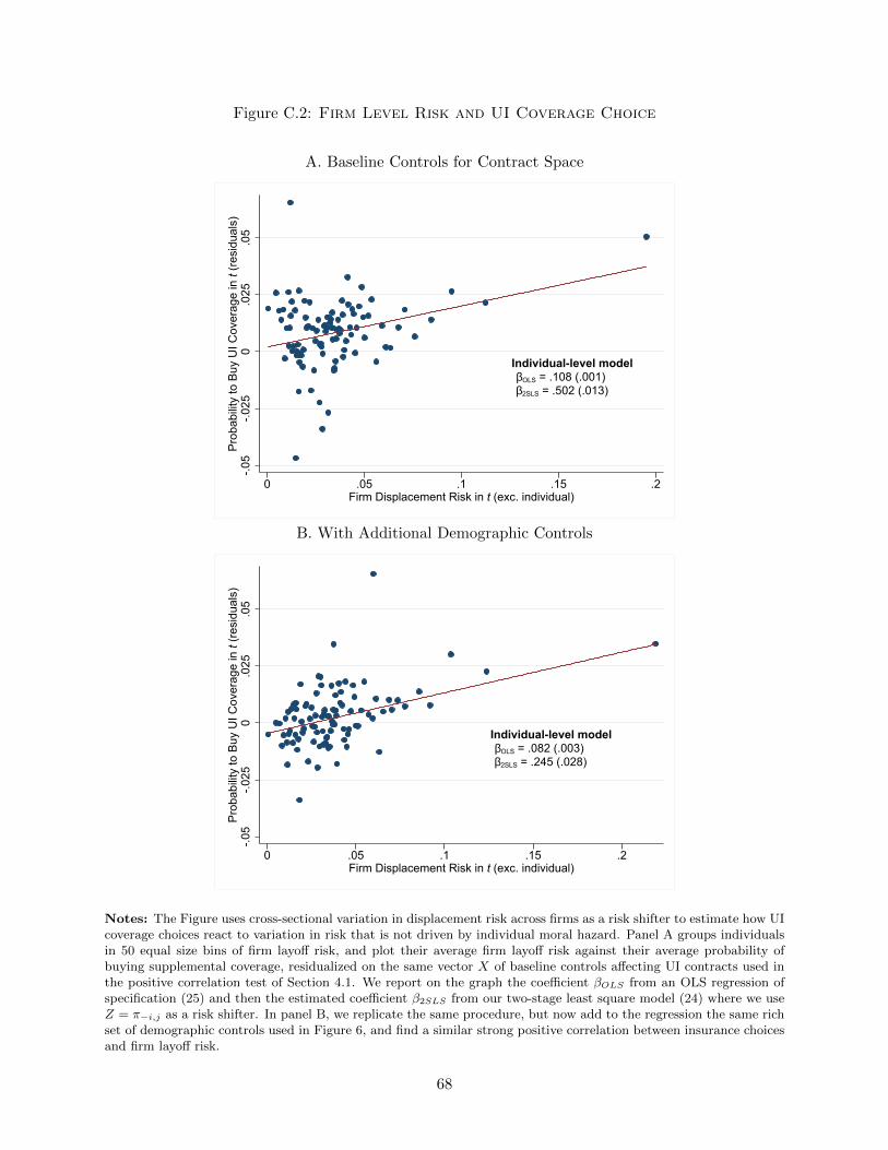
Figure C.2: Firm Level Risk and UI Coverage Choice

A. Baseline Controls for Contract Space

Individual-level modelβOLS = .108 (.001)β2SLS = .502 (.013)

-.05

-.025

0.0

25.0

5Pr

obab

ility

to B

uy U

I Cov

erag

e in

t (re

sidu

als)

0 .05 .1 .15 .2Firm Displacement Risk in t (exc. individual)

B. With Additional Demographic Controls

Individual-level modelβOLS = .082 (.003)β2SLS = .245 (.028)

-.05

-.025

0.0

25.0

5Pr

obab

ility

to B

uy U

I Cov

erag

e in

t (re

sidu

als)

0 .05 .1 .15 .2Firm Displacement Risk in t (exc. individual)

Notes: The Figure uses cross-sectional variation in displacement risk across firms as a risk shifter to estimate how UIcoverage choices react to variation in risk that is not driven by individual moral hazard. Panel A groups individualsin 50 equal size bins of firm layoff risk, and plot their average firm layoff risk against their average probability ofbuying supplemental coverage, residualized on the same vector X of baseline controls affecting UI contracts used inthe positive correlation test of Section 4.1. We report on the graph the coefficient βOLS from an OLS regression ofspecification (25) and then the estimated coefficient β2SLS from our two-stage least square model (24) where we useZ = π−i,j as a risk shifter. In panel B, we replicate the same procedure, but now add to the regression the same richset of demographic controls used in Figure 6, and find a similar strong positive correlation between insurance choicesand firm layoff risk.

68

Firm Switcher Design In this strategy, we use the panel dimension of the data to control for

the selection introduced by individual specific heterogeneity κi.

To this end, we focus on individuals who change firms (“switchers”). The employer-employee

matched data (RAMS ) registers all existing labor contracts on a monthly basis. We define a switch

as moving from having a labor contract with firm j (the origin firm) to having a contract with firm

k (the destination firm), without any recorded non-employment spell between these two contracts.

We focus on individuals with more than 1 year of tenure in the origin firm. Switchers experience

a change in their layoff risk coming from underlying variation in two risk shifters: their tenure

ranking changes, and so does their underlying firm layoff risk.

First, switchers experience a reduction in their relative tenure ranking, as they become the

“last-in” when they move to the destination firm. To document the magnitude of the variation in

relative tenure ranking and corresponding layoff risk, following a firm switch, we define year n = 0

as the year of a firm switch, and run, on the sample of firm switchers, event studies of the form:

Ti,n =∑k

δk · 1[n = k] + Z′iα+ εi,n (26)

where Tn denotes the tenure ranking of individual i in event year n, 1[n = k] are a set of event

time dummies, and Z is the vector of baseline controls affecting UI contracts defined in section

4.1. Figure C.3 displays the evolution of relative tenure ranking of switchers as a function of event

time by plotting the coefficients δk, taking event time n = −1 as the omitted category. The graph

confirms that relative tenure ranking decreases sharply at the moment of the firm switch.

Figure C.4 panel A explores how this variation in relative tenure ranking affects the probability

of displacement over event time n. To this effect, we estimate a similar event study specification

as in (26) where we use the probability of displacement πi in year t+ 1 as an outcome. The graph

shows that the displacement rate one year ahead increases sharply and significantly at the time of

the firm switch.

In Figure C.5 panel A, we run a similar event study specification with Di, a dummy for buying

the comprehensive UI coverage as an outcome. The figure shows that the probability of buying

the comprehensive coverage increases sharply by about 2.2 percentage points at the time of the

firm switch. On the graph, we also display the coefficient from the following two-stage least square

specification:

Di,n = κi + β2SLS · πi,n + Z′i,nα1 + εi,n

πi,n = νi + ζ · 1[n ≥ 0] + Z′i,nα2 + ηi,n(27)

where we use a dummy for having switched firm (1[n ≥ 0]) as risk shifter for individual displacement

probability πi,n and control for individual fixed-effects. This specification is estimated on the sample

of all workers who ever experience a firm switch between 2002 and 2006 and who have more than

1 year of tenure in the origin firm. β2SLS is positive and strongly significant, which again indicates

that the positive correlation tests are not simply picking up moral hazard responses to insurance

69

coverage.

While these event study specifications control for fixed underlying heterogeneity across individ-

uals that may affect their UI choices (κi), one concern with this original implementation of the firm

switchers design is that individuals are somewhat inert, and decide to reoptimize their UI choices

only at specific times, like, for instance, when they switch firm.

To mitigate the concern that the surge in UI coverage at the time of the switch is the result of

the specific timing of UI choices and not a response to the change in underlying risk, we exploit

additional variation in risk in the switchers design coming from changes in underlying firm layoff

risk. While all switchers experience an increase in their displacement probability due to the decline

in their tenure ranking, the effect of a switch on individual displacement probability exhibits large

differences according to whether their destination firm is much riskier (“positive shock”) or a lot

less risky (“negative shock”) than their origin firm. We therefore split the population of switchers

according to their rank in the distribution of ∆j,j′ π−i = π−i,j′−π−i,j , the change in their underlying

average firm layoff risk when moving from firm j to firm j′. In Figure C.4 panel B, we contrast

individuals in the bottom decile of ∆j,j′ π−i (large negative shock, i.e., individuals who experience

a large negative decline in their firm layoff risk, going from a high risk to a low risk firm), and

individuals in the top decile of ∆j,j′ π−i (large positive shock, i.e., individuals who experience a large

increase in their firm layoff risk going from a low risk to a high risk firm). The Figure confirms that

individuals experiencing a large positive shock in their firm layoff risk exhibit a significantly larger

increase, of about 2 percentage point, in their displacement probability at the time of the switch,

relative to individuals experiencing a large negative shock.

In panel B of Figure C.5, we now compare the evolution of insurance choices around firm switch

for individuals experiencing large positive vs large negative shocks. We run event study specification

(26) with Di, a dummy for buying the comprehensive UI coverage as an outcome, separately for

the sample of individuals experiencing large positive shocks and for the sample of individuals

experiencing large negative shocks. The graph indicates that the increase in the probability to buy

UI around firm switch is significantly larger (by about 1.5 percentage point) among individuals

moving to significantly more risky firms relative to those moving to less risky firms. We also report

on the graph the estimated coefficient β2SLS = .57 (.08) of the two-stage model:

Di,n = κi + β2SLS · πi,n +∑

k δk · 1[n = k] + Z′i,nα1 + εi,n

πi,n = νi + ζ · 1[n ≥ 0] ·∆π−i,j + Z′i,nα2 + ηi,n(28)

This model uses firm switch interacted with the change in average firm level layoff risk ∆π−i,j

as risk shifter for individual displacement probability. This model estimated on the sample of all

workers who ever experience a firm switch between 2002 and 2006 and who have more than 1 year

of tenure in the origin firm. The results suggest that the probability to buy the comprehensive

coverage is strongly correlated with average firm layoff risk, even after controlling for individual

unobserved heterogeneity with this switcher design strategy.

70

Figure C.3: Switchers Design: Relative Tenure Ranking as a Function of Event Time

Individualswitches firm

-.15

-.1-.0

50

.05

Rel

ativ

e Te

nure

Ran

k

-4 -3 -2 -1 0 1 2 3Event Time (years since/to switch)

Notes: The Figure focuses on “firm switchers”, i.e. individuals moving from having a labor contract with firm j tohaving a contract with firm k, without any recorded non-employment spell between these two contracts. We focuson individuals with more than 1 year of tenure in the origin firm. In this Figure we show that switchers experiencea variation in their layoff risk coming from underlying variation in their relative tenure ranking. Relative tenureranking affects displacement probability due to the strict enforcement of the Last-In-First-Out (LIFO) principle inSwedish labor laws. To follow the rules pertaining to the application of LIFO, relative tenure ranking is definedwithin each establishment times occupation group using the RAMS employer-employee data since 1985. The chartdisplays estimates of the event study specification (26) using relative tenure ranking as an outcome. The graph showsthat relative tenure ranking drops abruptly at the time of the firm switch. Panel A of Figure C.4 shows that thisdrop in tenure ranking translates in a significant increase in displacement risk.

71

Figure C.4: Firm Switchers - Displacement Rate in t+1 as a Function of Time to/sinceFirm Switch

A. All Switchers

Individualswitches firm

0.0

1.0

2.0

3.0

4.0

5D

ispl

acem

ent P

roba

bilit

y in

t+1

-4 -3 -2 -1 0 1 2 3Event Time (years since/to switch)

B. Switchers Experiencing Large Positive Firm Layoff Risk Shockvs Large Negative Firm Layoff Risk Shock

Individualswitches firm

0.0

2.0

4.0

6.0

8D

ispl

acem

ent P

roba

bilit

y in

t+1

-4 -3 -2 -1 0 1 2 3Event Time (years since/to switch)

Large negative shockLarge positive shock

Notes: The Figure focuses on “firm switchers”, i.e. individuals moving from having a labor contract with firm j tohaving a contract with firm k, without any recorded non-employment spell between these two contracts. We focuson individuals with more than 1 year of tenure in the origin firm. Switchers experience a variation in their layoff riskcoming from underlying variation in both risk shifters: their tenure ranking changes, and so does their underlyingfirm layoff risk. In panel A, we display estimates of the event study specification (26) using displacement risk int + 1 as an outcome. The graph shows that the displacement risk increases sharply and significantly at the timeof the firm switch. In panel B, we split the population of switchers according to their rank in the distribution of∆j,j′π−i = π−i,j′ − π−i,j , the change in their underlying firm risk when moving from firm j to firm j′. We focus onindividuals in the bottom decile of ∆j,j′π−i (large negative shock, i.e., individuals going from a high risk to a lowrisk firm), and individuals in the top decile of ∆j,j′π−i (large positive shock).

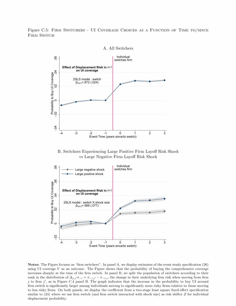
Figure C.5: Firm Switchers - UI Coverage Choices as a Function of Time to/sinceFirm Switch

A. All Switchers

Individualswitches firm

Effect of Displacement Risk in t+1on UI coverage

2SLS model : switchβ2SLS=.872 (.024)

-.04

-.02

0.0

2.0

4.0

6Pr

obab

ility

to B

uy U

I Cov

erag

e

-4 -3 -2 -1 0 1 2 3Event Time (years since/to switch)

B. Switchers Experiencing Large Positive Firm Layoff Risk Shockvs Large Negative Firm Layoff Risk Shock

Individualswitches firm

Effect of Displacement Risk in t+1on UI coverage

2SLS model : switch X shock size β2SLS=.569 (.077)

-.02

0.0

2.0

4.0

6.0

8Pr

obab

ility

to B

uy U

I Cov

erag

e

-4 -3 -2 -1 0 1 2 3Event Time (years since/to switch)

Large negative shockLarge positive shock

Notes: The Figure focuses on “firm switchers”. In panel A, we display estimates of the event study specification (26)using UI coverage V as an outcome. The Figure shows that the probability of buying the comprehensive coverageincreases sharply at the time of the firm switch. In panel B, we split the population of switchers according to theirrank in the distribution of ∆j,j′π−i = π−i,j′ − π−i,j , the change in their underlying firm risk when moving from firmj to firm j′, as in Figure C.4 panel B. The graph indicates that the increase in the probability to buy UI aroundfirm switch is significantly larger among individuals moving to significantly more risky firms relative to those movingto less risky firms. On both panels, we display the coefficient from a two-stage least square fixed-effect specificationsimilar to (24) where we use firm switch (and firm switch interacted with shock size) as risk shifter Z for individualdisplacement probability.

C.3 Risk Shifter & UI Choices II: Layoff Notifications and LIFO

The previous section suggests a strong correlation between firm layoff risk and UI choices, indicative

of the presence of significant adverse selection. As explained above though, firm layoff risk may be

correlated with willingness-to-pay for UI, either through unobserved individual specific heterogene-

ity (κi) or unobserved firm specific heterogeneity (ρj). The firm switcher design above deals with

individual specific heterogeneity (κi), but may still pick up selection on firm level heterogeneity ρj

if firm heterogeneity is correlated with ∆π−i,j .

We now show how layoff notifications and the application of the Last-In-First-Out (LIFO)

principle enables to identify the effect of predictable risk on UI choices controlling jointly for

firm level heterogeneity ρj and individual level heterogeneity κi. We leverage the fact that layoff

notifications and LIFO creates variation in layoff risk both within firm and across individuals over

time.

In section 2.1, we described the institutional details of the layoff notification system and its

interaction with the LIFO rule. We also explained and demonstrated in Appendix A, that layoff

notifications signal a significant change in a firm layoff risk. In particular, we reported in Figure

A.2 that the displacement probability of workers increases sharply and significantly around the first

layoff notification event in the history of the firm. We also showed in Figure A.1 panel B that the

effect of a layoff notification on displacement probability is strongly heterogenous depending on

the relative tenure ranking of workers. Workers with relative tenure ranking below .5 have a much

higher probability of being laid-off following a layoff notification than workers with relative tenure

ranking above .5.

We now show how UI choices correlate with this variation in risk stemming from the interaction

between a notification event and relative tenure ranking. We follow the same event study empirical

approach as in section Appendix A around the event of a layoff notification. We define event year

n as the year to/since the firm emits its first layoff notification.

Our sample is the panel of workers who are employed in the firm at the date this layoff notifi-

cation is emitted to the PES. All these workers constitute our treatment group. We follow, as in

Appendix A a matching strategy and create a control panel of workers. To do this, we use nearest-

neighbor matching to select a set of firms that are similar, along a set of observable characteristics,

to the firms emitting a layoff notification, but never emit a layoff notification.49 We allocate to the

matched firm in the control group a placebo event date equal to the layoff notification date of her

nearest-neighbor in the treated group of firms. We then select workers that are in the control firm

at the time of the placebo event date to create our matched panel of control individuals.

In Figure C.6 we split the sample by tenure ranking at the time the layoff notification is emitted

and report the evolution of the average fraction of individuals buying the supplemental coverage

in our treatment group and in the matched control group.50 Panel A of Figure C.6 reports the

49The covariates used for matching are the number of employees, the 4 digit sector codes of the firm, the averageearnings and average years of education of workers in the firm.

50For control workers we use their tenure ranking at the time of the placebo layoff notification.

74

evolution of the fraction buying the supplemental UI coverage for workers with relative tenure

ranking below 50% in year n = 0. The graph shows that UI coverage increases significantly

among the treated group, starting one year before the layoff notification is sent, which suggests

the existence of some degree of private information among workers regarding the timing of the

layoff notification. In panel B, we report the evolution of UI choices for the sample of workers with

relative tenure ranking above 50% in year n = 0. The graph displays no sign of variation in the

fraction of individuals buying the comprehensive coverage around the notification event.

On both panels, we also report estimates β of the reduced form specification:

Di,n = κi + ρj + β · 1[n ≥ 0] · 1[T = 1] + θ · 1[n ≥ 0] + Z′i,nα1 + εi,n (29)

as well as estimates β2SLS from the following two-stage specification:

Di,n = κi + ρj + β2SLS · πi,n +∑

k δk · 1[n = k] + Z′i,nα1 + εi,n

πi,n = νi + γj + ζ · 1[n ≥ 0] · 1[T = 1] + θ · 1[n ≥ 0] + Z′i,nα2 + ηi,n(30)

The above two-stage model specification uses variation in risk stemming from being in a firm

having emitted a layoff notification, and controls for both individual fixed effects (κi) and firm

fixed effects (ρj). The comparison between the estimates for the low vs high tenure ranking sample

further exploits the additional layer of variation in displacement risk coming from the interaction

between a notification event and relative tenure ranking. Results show that individuals with low

tenure ranking strongly respond to the variation in risk arising from a layoff notification and are

significantly more likely to buy the comprehensive coverage as a result: β2SLS = .84 (.21). To the

contrary, the UI choices of individuals with high tenure ranking do not significantly respond to a

layoff notification.

Summary of evidence Taken together, the evidence from this appendix strongly suggests that

UI choices do significantly respond to the various sources of variations in individuals’ predictable

unemployment risk. The different strategies clearly differ in terms of the way they control for

underlying selection on unobserved heterogeneity into the comprehensive coverage, as well as in

terms of the population of compliers. Yet, we systematically find a strong positive and significant

relationship between the probability to buy the comprehensive coverage and the observable risk

shifters entering our predicted risk model. This overall confirms that the strong correlation between

predictable risk and UI choices documented in section 4.2 does capture the presence of significant

adverse selection into the comprehensive coverage.

75

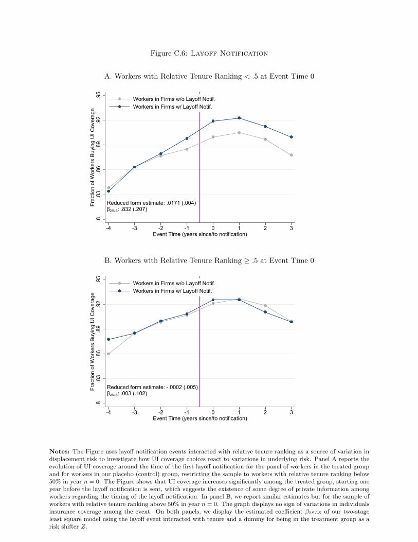
Figure C.6: Layoff Notification

A. Workers with Relative Tenure Ranking < .5 at Event Time 0

Reduced form estimate: .0171 (.004)β2SLS: .832 (.207)

.8.8

3.8

6.8

9.9

2.9

5Fr

actio

n of

Wor

kers

Buy

ing

UI C

over

age

-4 -3 -2 -1 0 1 2 3Event Time (years since/to notification)

Workers in Firms w/o Layoff Notif.Workers in Firms w/ Layoff Notif.

B. Workers with Relative Tenure Ranking ≥ .5 at Event Time 0

Reduced form estimate: -.0002 (.005)β2SLS: .003 (.102)

.8.8

3.8

6.8

9.9

2.9

5Fr

actio

n of

Wor

kers

Buy

ing

UI C

over

age

-4 -3 -2 -1 0 1 2 3Event Time (years since/to notification)

Workers in Firms w/o Layoff Notif.Workers in Firms w/ Layoff Notif.

Notes: The Figure uses layoff notification events interacted with relative tenure ranking as a source of variation indisplacement risk to investigate how UI coverage choices react to variations in underlying risk. Panel A reports theevolution of UI coverage around the time of the first layoff notification for the panel of workers in the treated groupand for workers in our placebo (control) group, restricting the sample to workers with relative tenure ranking below50% in year n = 0. The Figure shows that UI coverage increases significantly among the treated group, starting oneyear before the layoff notification is sent, which suggests the existence of some degree of private information amongworkers regarding the timing of the layoff notification. In panel B, we report similar estimates but for the sample ofworkers with relative tenure ranking above 50% in year n = 0. The graph displays no sign of variations in individualsinsurance coverage among the event. On both panels, we display the estimated coefficient β2SLS of our two-stageleast square model using the layoff event interacted with tenure and a dummy for being in the treatment group as arisk shifter Z.

Appendix D Price Variation: Additional Material

In this appendix we present additional results using the 2007 price variation to identify adverse

selection:

(i) we present further non-parametric evidence of adverse selection using additional risk outcomes

(ii) we show how adverse selection would survive the inclusion of many unused demographic

observables in the Swedish UI policy

(iii) we provide evidence showing that our ranking of willingness-to-pay for the comprehensive

coverage correlates strongly with proxies for the value of unemployment insurance and for

risk preferences.

(iv) we address potential concerns, such as inertia, to the validity of our ranking of individuals by

willingness-to-pay.

Alternative risk outcomes In our baseline analysis of the 2007 reform in section 5, we use total

number of days unemployed in 2008 as our main outcome. Here, we show that our estimates of

adverse selection are again robust to using alternative risk outcomes. We look at the displacement

probability in t+1, t+2,... up to t+5. To control for observables Z, we model the probability of

displacement as a probit:

E(π|Z) = Φ(Z ′β +∑j

αj · 1[D = j]) (31)

where Φ(.) is the standard normal c.d.f.

In Figure D.1 we report the correlation between willingness-to-pay in 2007 and displacement

outcomes in t+1, t+2,... up to t+5. We report for each year the semi elasticity

Semit+kM(p) =E(πt+k|Z,D = M)− E(πt+k|Z,D = 0)

E(πt+k|Z,D = 0)

of the displacement probability in t+ k for the marginals D = M relative to the individuals in the

basic coverage throughout D = 0. The figure reveals that the correlation between unemployment

risk and willingness-to-pay decreases rapidly as we consider later years, but remains statistically

significant up to five years.

Role of Unpriced Heterogeneity The 2007 price reform allows us to investigate how much of

the risk-based selection is driven by selection on specific unpriced observables correlated with risk.

We do so by sequentially including in specification (16) a set of controlsX: dummies for age, gen-

der, marital status, education (four categories), industry (1-digit code) and and wealth level (quar-

tiles). We then report for each specification the semi-elasticity SemiXM(p) = E(π|Z,X,D=M)−E(π|Z,X,D=0)E(π|Z,X,D=0) .

Interestingly, the semi-elasticity increases compared to our baseline when including age as a

control. Age is therefore a driver of advantageous selection into UI. Adding rich sets of controls

77

Figure D.1: Price Variation: Using Displacement Probability as a Risk Outcome

0.2

5.5

.75

11

.25

Se

mi−

ela

sticity R

ela

tive

to

Alw

ays U

nin

su

red

2008 2009 2010 2011 2012Year of Displacement Probability

Notes: The Figure reports the correlation between willingness-to-pay in 2007 and realized displacement outcomesin 2008, 2009,.. up to 2012. We report for each year, the semi-elasticity Semit+kM(p) of the displacement probability inyear t+ k for the marginals M relative to the individuals from group 0.

78

for education, industry, occupation and wealth decreases the estimated correlation only slightly,

indicating that there is little risk-related selection along these margins.

Overall, this suggests that demographic characteristics, and age especially, provide advantageous

selection on average, such that if contracts were differentiated along these observable dimensions,

adverse selection into comprehensive coverage would actually be more severe.

Furthermore, controlling for these unpriced observables does not exhaust risk-based selection

in the supplemental UI coverage. In other words, even if the supplemental coverage policy were

to price this rich set of observable characteristics, a significant amount of adverse selection would

remain.

Figure D.2: Price Variation: Role of Unpriced Heterogeneity

0.5

11.

52

2.5

Sem

i-Ela

stic

ity o

f Ris

k M

easu

re w

.r.t I

nsur

ance

Cho

ice

Baseline + Age + Gender + FamilyType

+ Education + Industry + Occupation + NetWealth

Notes: The Figure explores to what extent estimated adverse selection using the 2007 price variation is driven byselection on observable characteristics that are unpriced in the Swedish UI system. We report the semi-elasticitySemiXM(p) of the number of days spent unemployed in 2008 for the marginals M relative to the individuals from group0. We start with the baseline estimate only controlling for the characteristics affecting the actual UI policy, and showhow the semi-elasticity evolves as we add sequentially more characteristics to the vector of controls X. We start byadding demographic controls (age, then gender, and marital status), then controls for skills and other labor marketcharacteristics (controls for education (four categories), industry (1-digit code), occupation (1-digit code) and wealthlevel (quartiles).

79

Selection on preferences and value of UI The 2007 price reform also allows to investigate

patterns of selection along dimensions other than risk. In Figure D.3, we examine how character-

istics that determine the value of unemployment insurance and proxy for risk preferences correlate

with willingness-to-pay for insurance revealed by the 2007 price variation. Panel A correlates the

level of individuals’ net wealth in 2006 in thousands of SEK with their willingness-to-pay control-

ling for age. Individuals with larger net wealth have more means to smooth consumption in case

of displacement, and as a result, should value extra coverage less. The graph indeed confirms the

presence of a clear monotonic relationship between net wealth and willingness-to-pay: individuals

from group 0 have significantly larger net wealth than the marginals M , who have significantly

more net wealth than the individuals from group 1. In panel B, we probe into the potential amount

of selection based on risk-preferences. To proxy for risk aversion, we use the fraction of total net

wealth invested in risky assets (stocks). The graph shows that the individuals in comprehensive

coverage have a significantly larger fraction of risky assets in their portfolio than the marginals and

the individuals in basic coverage, conditional on net wealth. This evidence is in line with more

risk-averse individuals valuing the extra coverage more.

80

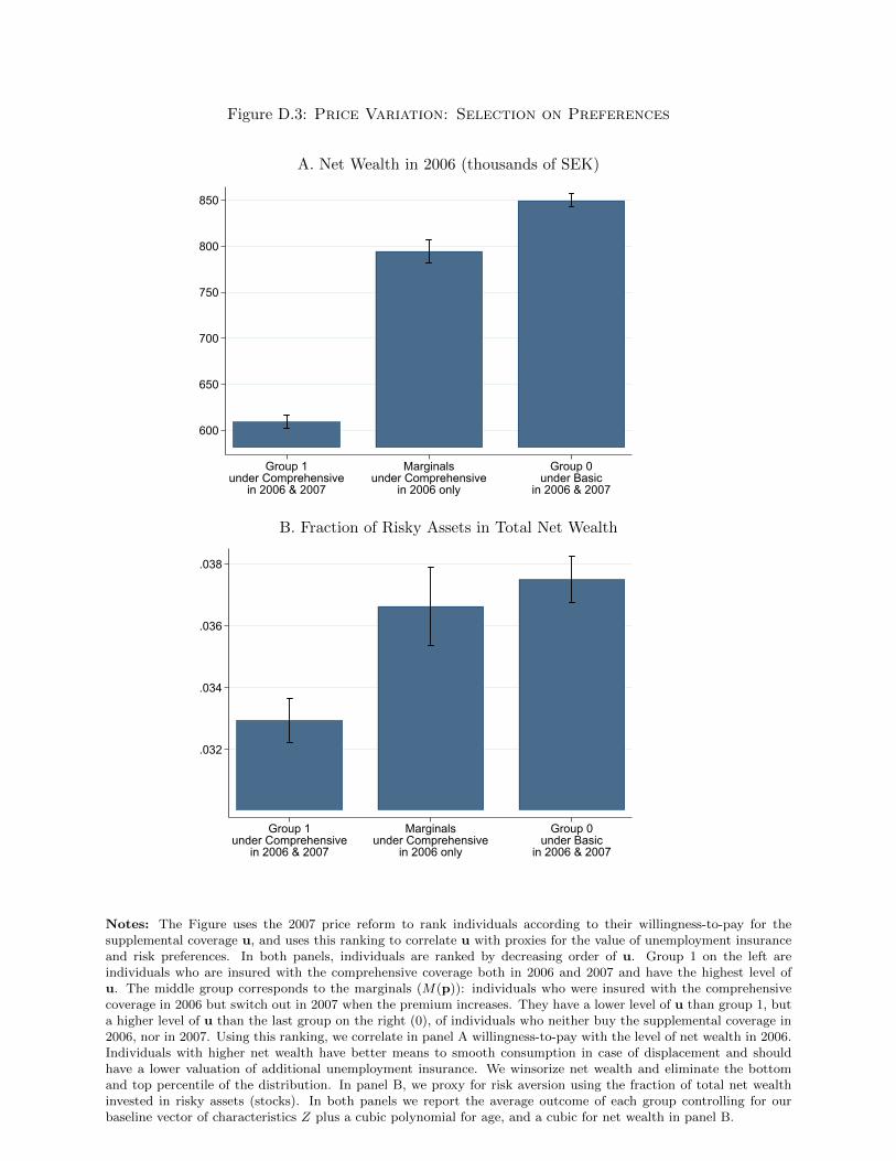
Figure D.3: Price Variation: Selection on Preferences

A. Net Wealth in 2006 (thousands of SEK)

600

650

700

750

800

850

Group 1under Comprehensive

in 2006 & 2007

Marginalsunder Comprehensive

in 2006 only

Group 0under Basic

in 2006 & 2007

B. Fraction of Risky Assets in Total Net Wealth

.032

.034

.036

.038

Group 1under Comprehensive

in 2006 & 2007

Marginalsunder Comprehensive

in 2006 only

Group 0under Basic

in 2006 & 2007

Notes: The Figure uses the 2007 price reform to rank individuals according to their willingness-to-pay for thesupplemental coverage u, and uses this ranking to correlate u with proxies for the value of unemployment insuranceand risk preferences. In both panels, individuals are ranked by decreasing order of u. Group 1 on the left areindividuals who are insured with the comprehensive coverage both in 2006 and 2007 and have the highest level ofu. The middle group corresponds to the marginals (M(p)): individuals who were insured with the comprehensivecoverage in 2006 but switch out in 2007 when the premium increases. They have a lower level of u than group 1, buta higher level of u than the last group on the right (0), of individuals who neither buy the supplemental coverage in2006, nor in 2007. Using this ranking, we correlate in panel A willingness-to-pay with the level of net wealth in 2006.Individuals with higher net wealth have better means to smooth consumption in case of displacement and shouldhave a lower valuation of additional unemployment insurance. We winsorize net wealth and eliminate the bottomand top percentile of the distribution. In panel B, we proxy for risk aversion using the fraction of total net wealthinvested in risky assets (stocks). In both panels we report the average outcome of each group controlling for ourbaseline vector of characteristics Z plus a cubic polynomial for age, and a cubic for net wealth in panel B.

Robustness Our partition of the population in terms of willingness-to-pay implicitly assumes

that u is constant over time, or to be more precise that the ranking of individuals’ willingness-

to-pay is the same in 2006 and 2007. In practice u may change over time, due for instance to

idiosyncratic shocks to risk, or preferences, thus creating a flow of individuals switching out of the

comprehensive plan, even absent price changes. Appendix Figure D.4 provides evidence that the

flow of individuals who switch out of the supplemental coverage was in fact very small prior to the

2007 price reform, but experienced a sudden surge in 2007. This alleviates the concern that our

ranking of individuals by willingness-to-pay is confounded by underlying changes in individuals’

preferences or risks.

We also note that our partition of the population ignores a negligible fourth group of individuals,

who were not buying the comprehensive plan in 2006, but switched in the comprehensive plan in

2007. The size of this group is seven times smaller than the group of individuals switching out of

the comprehensive plan in 2007. The ranking of this fourth group in terms of willingness-to-pay

is also ambiguous, as one would need to include idiosyncratic shocks to u to account for the fact

that these individuals switched in the comprehensive coverage in 2007 despite the increase in prices

p. We display in Appendix Figure D.4 the evolution of the flow of individuals not buying the

comprehensive plan in t − 1 but switching in the comprehensive plan in t. The graph shows that

this flow of individuals was small prior to 2007, and equivalent in size to the flow of individuals

switching out, hence the stability in the fraction of individuals insured. The flow of individuals

switching in seems to decrease with the 2007 reform, but only slightly. The average unemployment

risk of the workers switching into the comprehensive plan was the highest among the four groups

throughout this period.

82

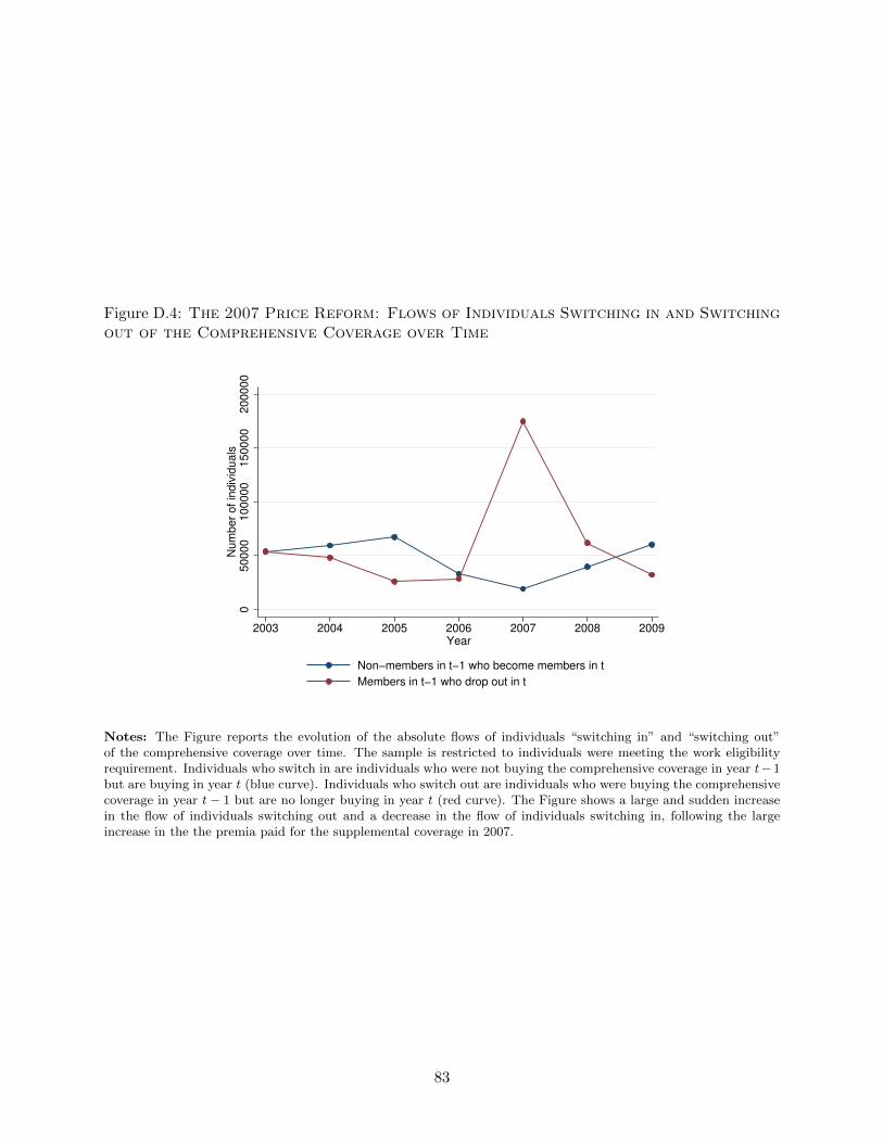
Figure D.4: The 2007 Price Reform: Flows of Individuals Switching in and Switchingout of the Comprehensive Coverage over Time

050000

100000

150000

200000

Num

ber

of in

div

iduals

2003 2004 2005 2006 2007 2008 2009Year

Non−members in t−1 who become members in t

Members in t−1 who drop out in t

Notes: The Figure reports the evolution of the absolute flows of individuals “switching in” and “switching out”of the comprehensive coverage over time. The sample is restricted to individuals were meeting the work eligibilityrequirement. Individuals who switch in are individuals who were not buying the comprehensive coverage in year t−1but are buying in year t (blue curve). Individuals who switch out are individuals who were buying the comprehensivecoverage in year t− 1 but are no longer buying in year t (red curve). The Figure shows a large and sudden increasein the flow of individuals switching out and a decrease in the flow of individuals switching in, following the largeincrease in the the premia paid for the supplemental coverage in 2007.

83

Inertia Inertia is a potentially important behavioral friction, which has been shown to be ex-

tremely relevant in other social insurance contexts, such as health insurance. We investigate here

the role of inertia and how it affects adverse selection identified in the context of the 2007 price

variation. In line with the existing the literature (e.g., Handel (2013)), we use job switchers to

proxy for differential exposure to inertia. New employees in a firm arguably face a more active

choice environment than existing employees. The former have to reoptimize many choices, while

the latter remain in a more passive choice environment. In practice, Figure C.7 above confirms

that switching job is indeed associated with a significant change in insurance choices.

In Figure D.5 below, we start by looking at how the price reform of 2007 affected insurance

choices for individuals in active choice environments (job switchers) relative to individuals in passive

choice environments (job stayers). We find that the 2007 price reform immediately decreased the

demand for the comprehensive coverage, in similar proportions, in both the active and the more

passive choice environment. But we do find a larger response one year after (in 2008) for job

switchers than for non-switchers, which suggests the presence of inertia. Overall, though, the

graph suggest that inertia plays a relatively limited role in our setting: individuals in passive choice

environments reacted strongly to the reform, and their long run demand response is quite similar

to that of individuals facing more active choice environments.

In Figure D.6, we further investigate whether the adverse selection created by these demand

responses is different for individuals in active vs passive choice environments. We report the semi-

elasticity of the predicted risk πj , j ∈ {0, 1} of marginals versus individuals always in the basic

coverage, splitting the sample by active vs passive choice environment in 2007:

SemiπjM(p) =

E(πj |Z,D = M)− E(πj |Z,D = 0)

E(πj |Z,D = 0)

where Z is a vector of characteristics affecting the contract space. We find that the adverse selection

identified by the 2007 price reform is slightly larger for predicted risk in the basic coverage for

workers observed in active compared to workers observed in passive choice environment. But we

do not find any significant difference in adverse selection for risk in the comprehensive coverage.

Put together, this evidence suggests that inertia does not seem to critically affect our estimates

of the demand and marginal cost curves. It is worth noting though that the relatively modest

inertia we find is likely due to the fact that the 2007 reform was large, and salient.

84

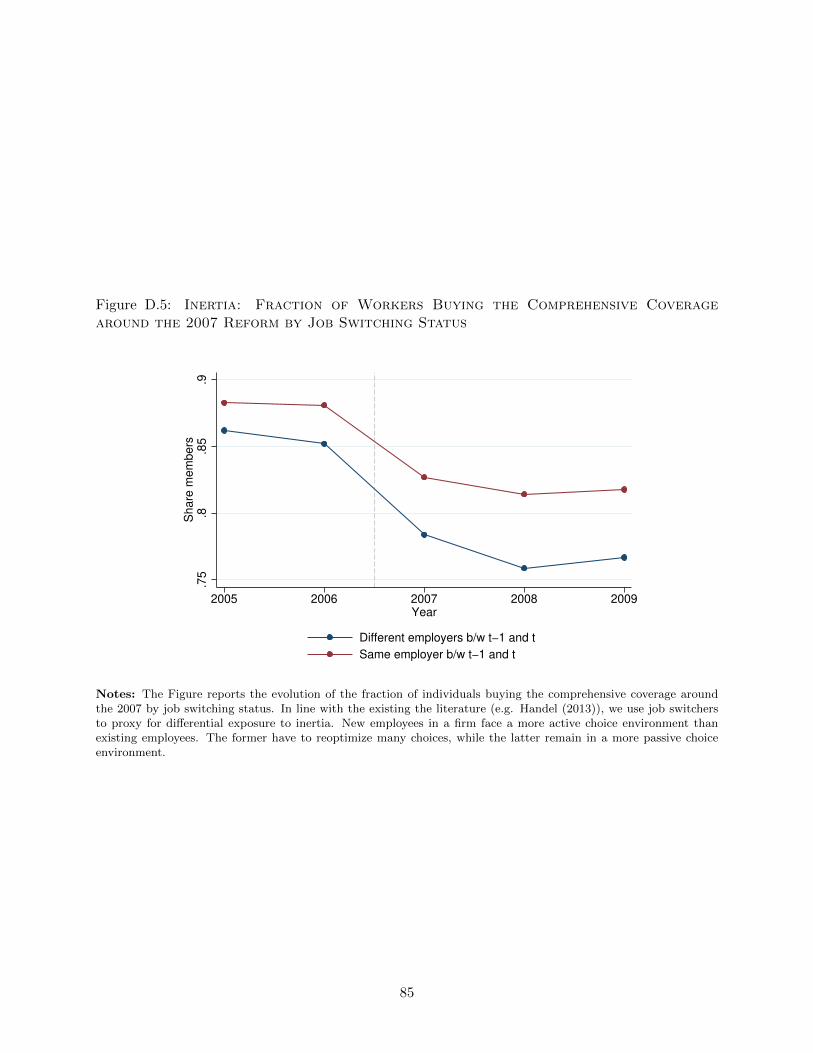
Figure D.5: Inertia: Fraction of Workers Buying the Comprehensive Coveragearound the 2007 Reform by Job Switching Status

.75

.8.8

5.9

Share

mem

bers

2005 2006 2007 2008 2009Year

Different employers b/w t−1 and t

Same employer b/w t−1 and t

Sample: Workers employed in t−1 and t, ages 25−60 in year t.Share switchers: .135

Notes: The Figure reports the evolution of the fraction of individuals buying the comprehensive coverage aroundthe 2007 by job switching status. In line with the existing the literature (e.g. Handel (2013)), we use job switchersto proxy for differential exposure to inertia. New employees in a firm face a more active choice environment thanexisting employees. The former have to reoptimize many choices, while the latter remain in a more passive choiceenvironment.

85

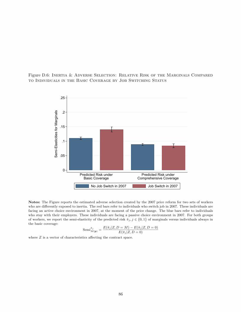
Figure D.6: Inertia & Adverse Selection: Relative Risk of the Marginals Comparedto Individuals in the Basic Coverage by Job Switching Status

0

.05

.1

.15

.2

.25

Sem

i-Ela

stic

ities

for M

argi

nals

Predicted Risk underBasic Coverage

Predicted Risk underComprehensive Coverage

No Job Switch in 2007 Job Switch in 2007

Notes: The Figure reports the estimated adverse selection created by the 2007 price reform for two sets of workerswho are differently exposed to inertia. The red bars refer to individuals who switch job in 2007. These individuals arefacing an active choice environment in 2007, at the moment of the price change. The blue bars refer to individualswho stay with their employers. These individuals are facing a passive choice environment in 2007. For both groupsof workers, we report the semi-elasticity of the predicted risk πj , j ∈ {0, 1} of marginals versus individuals always inthe basic coverage:

Semiπj

M(p) =E(πj |Z,D = M)− E(πj |Z,D = 0)

E(πj |Z,D = 0)

where Z is a vector of characteristics affecting the contract space.

86

Appendix E Benefit Variation: Additional Material

In this appendix we provide additional material regarding our RKD estimation of the effect of

benefit variation on insurance choices and risk-based selection:

(i) we present results assessing the validity of our RK design.

(ii) we present results assessing the sensitivity of our RKD estimates.

Table E.2 provides the summary statistics for the sample used for the RKD analysis.

E.1 Assessing Validity of the RK Design

The key identifying assumption of the RK design is the existence of a smooth relationship at the

threshold w = 850SEK between the assignment variable and any pre-determined characteristics

affecting the demand for insurance. To assess the credibility of this assumption, we conduct two

types of analysis [see also Kolsrud et al. [2018]].

Smoothness of the distribution of the assignment variable at the kink First, we focus

on the probability density function of the assignment variable, to detect manipulation or lack of

smoothness around the kink that could indicate the presence of selection. Figure E.1 shows that

the pdf of daily wage does not exhibit a discontinuity nor lack of smoothness at the kink, which is

confirmed by the results of formal McCrary tests.

Covariate Tests Second, we investigate the presence of potential selection along observable char-

acteristics around the kink. For this purpose, instead of looking at each characteristics in isolation,

we aggregate them in a covariate index. The index is a linear combination of a vector of charac-

teristics X that correlate with our outcomes of interest for the RKD, which includes age, gender,

level of education, region, family type and industry. The coefficients in the linear combination are

obtained from a regression of the outcome variable on these covariates. In Figure E.2, we display

the relationship between this covariate index and the assignment variable for our three outcomes

of interest: the choice of coverage, and the predicted risk under basic and comprehensive coverage.

The relationship between the index and daily wage appears smooth around the 850SEK threshold.

Yet, formal tests of non-linearity suggest the presence of a significant (although economically small)

kink at the threshold for insurance choice. But for predicted risk, we do not find any significant

non-linearity in the covariate index at the kink.

87

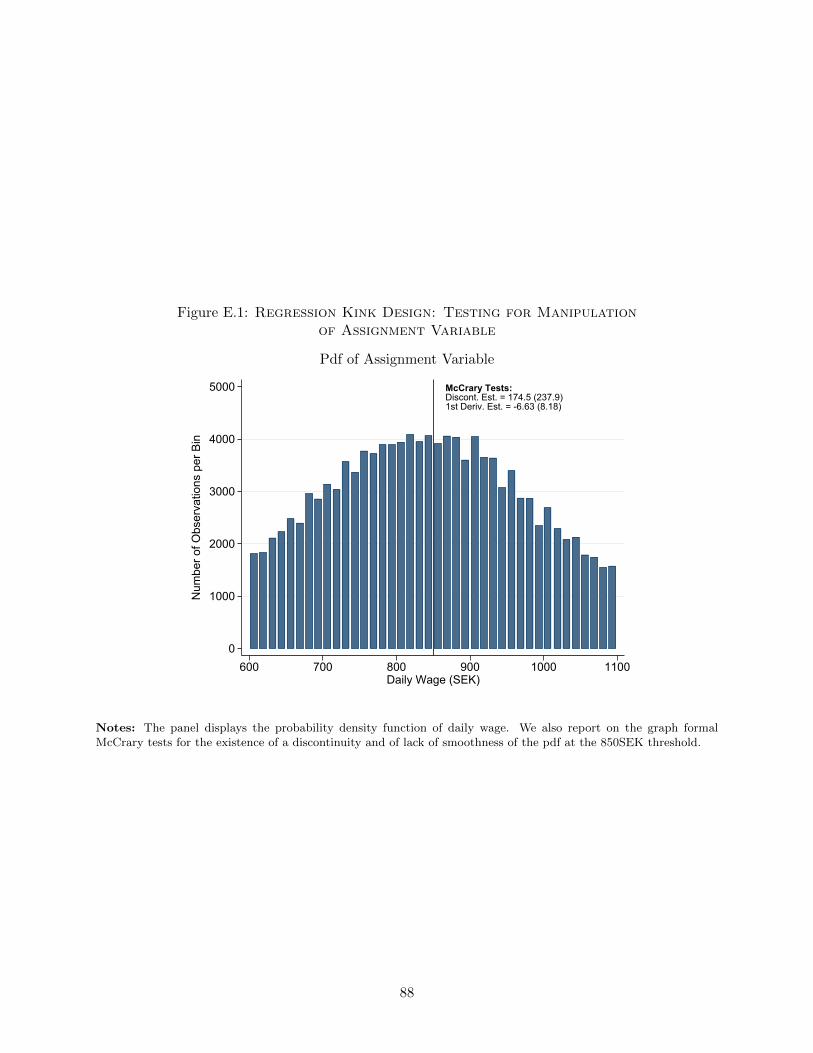
Figure E.1: Regression Kink Design: Testing for Manipulationof Assignment Variable

Pdf of Assignment Variable

McCrary Tests:Discont. Est. = 174.5 (237.9)1st Deriv. Est. = -6.63 (8.18)

0

1000

2000

3000

4000

5000

Num

ber o

f Obs

erva

tions

per

Bin

600 700 800 900 1000 1100Daily Wage (SEK)

Notes: The panel displays the probability density function of daily wage. We also report on the graph formalMcCrary tests for the existence of a discontinuity and of lack of smoothness of the pdf at the 850SEK threshold.

88

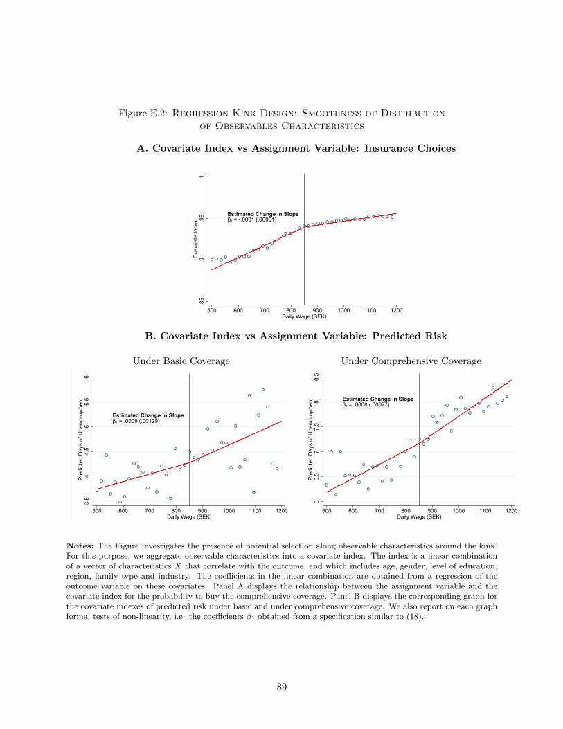
Figure E.2: Regression Kink Design: Smoothness of Distributionof Observables Characteristics

A. Covariate Index vs Assignment Variable: Insurance Choices

Estimated Change in Slopeβ1 = -.0001 (.00001)

.85

.9.9

51

Coa

vria

te In

dex

500 600 700 800 900 1000 1100 1200Daily Wage (SEK)

B. Covariate Index vs Assignment Variable: Predicted Risk

Under Basic Coverage Under Comprehensive Coverage

Estimated Change in Slopeβ1 = .0009 (.00129)

3.5

44.

55

5.5

6Pr

edic

ted

Day

s of

Une

mpl

oym

ent

500 600 700 800 900 1000 1100 1200Daily Wage (SEK)

Estimated Change in Slopeβ1 = .0008 (.00077)

66.

57

7.5

88.

5Pr

edic

ted

Day

s of

Une

mpl

oym

ent

500 600 700 800 900 1000 1100 1200Daily Wage (SEK)

Notes: The Figure investigates the presence of potential selection along observable characteristics around the kink.For this purpose, we aggregate observable characteristics into a covariate index. The index is a linear combinationof a vector of characteristics X that correlate with the outcome, and which includes age, gender, level of education,region, family type and industry. The coefficients in the linear combination are obtained from a regression of theoutcome variable on these covariates. Panel A displays the relationship between the assignment variable and thecovariate index for the probability to buy the comprehensive coverage. Panel B displays the corresponding graph forthe covariate indexes of predicted risk under basic and under comprehensive coverage. We also report on each graphformal tests of non-linearity, i.e. the coefficients β1 obtained from a specification similar to (18).

89

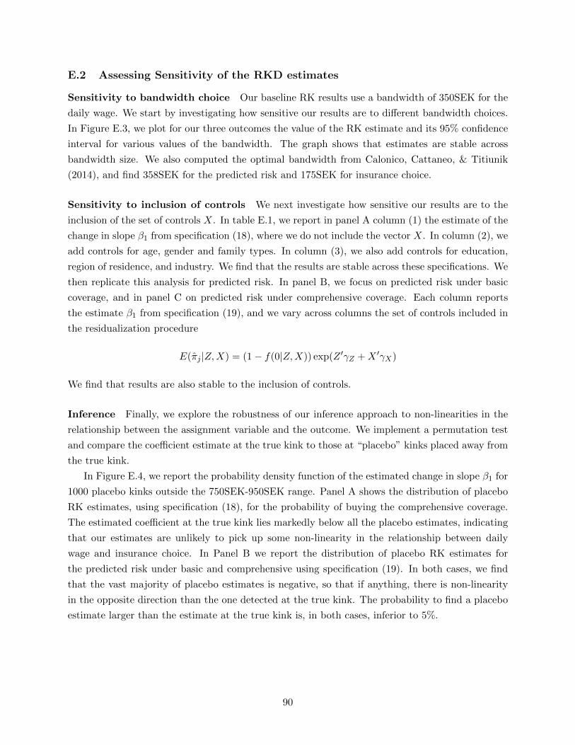
E.2 Assessing Sensitivity of the RKD estimates

Sensitivity to bandwidth choice Our baseline RK results use a bandwidth of 350SEK for the

daily wage. We start by investigating how sensitive our results are to different bandwidth choices.

In Figure E.3, we plot for our three outcomes the value of the RK estimate and its 95% confidence

interval for various values of the bandwidth. The graph shows that estimates are stable across

bandwidth size. We also computed the optimal bandwidth from Calonico, Cattaneo, & Titiunik

(2014), and find 358SEK for the predicted risk and 175SEK for insurance choice.

Sensitivity to inclusion of controls We next investigate how sensitive our results are to the

inclusion of the set of controls X. In table E.1, we report in panel A column (1) the estimate of the

change in slope β1 from specification (18), where we do not include the vector X. In column (2), we

add controls for age, gender and family types. In column (3), we also add controls for education,

region of residence, and industry. We find that the results are stable across these specifications. We

then replicate this analysis for predicted risk. In panel B, we focus on predicted risk under basic

coverage, and in panel C on predicted risk under comprehensive coverage. Each column reports

the estimate β1 from specification (19), and we vary across columns the set of controls included in

the residualization procedure

E(πj |Z,X) = (1− f(0|Z,X)) exp(Z ′γZ +X ′γX)

We find that results are also stable to the inclusion of controls.

Inference Finally, we explore the robustness of our inference approach to non-linearities in the

relationship between the assignment variable and the outcome. We implement a permutation test

and compare the coefficient estimate at the true kink to those at “placebo” kinks placed away from

the true kink.

In Figure E.4, we report the probability density function of the estimated change in slope β1 for

1000 placebo kinks outside the 750SEK-950SEK range. Panel A shows the distribution of placebo

RK estimates, using specification (18), for the probability of buying the comprehensive coverage.

The estimated coefficient at the true kink lies markedly below all the placebo estimates, indicating

that our estimates are unlikely to pick up some non-linearity in the relationship between daily

wage and insurance choice. In Panel B we report the distribution of placebo RK estimates for

the predicted risk under basic and comprehensive using specification (19). In both cases, we find

that the vast majority of placebo estimates is negative, so that if anything, there is non-linearity

in the opposite direction than the one detected at the true kink. The probability to find a placebo

estimate larger than the estimate at the true kink is, in both cases, inferior to 5%.

90

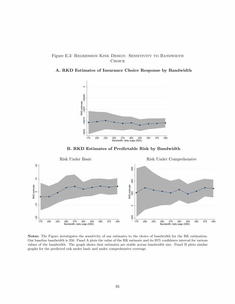
Figure E.3: Regression Kink Design: Sensitivity to BandwidthChoice

A. RKD Estimates of Insurance Choice Response by Bandwidth

-.000

2-.0

0015

-.000

1-.0

0005

0R

KD e

stim

ate

175 200 225 250 275 300 325 350 375 400Bandwidth: daily wage (SEK)

B. RKD Estimates of Predictable Risk by Bandwidth

Risk Under Basic Risk Under Comprehensive

-.02

-.01

0.0

1.0

2R

KD e

stim

ate

175 200 225 250 275 300 325 350 375 400Bandwidth: daily wage (SEK)

-.002

0.0

02.0

04.0

06R

KD e

stim

ate

175 200 225 250 275 300 325 350 375 400Bandwidth: daily wage (SEK)

Notes: The Figure investigates the sensitivity of our estimates to the choice of bandwidth for the RK estimation.Our baseline bandwidth is 350. Panel A plots the value of the RK estimate and its 95% confidence interval for variousvalues of the bandwidth. The graph shows that estimates are stable across bandwidth size. Panel B plots similargraphs for the predicted risk under basic and under comprehensive coverage.

91

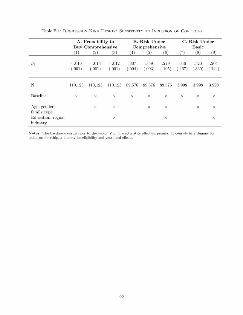
Table E.1: Regression Kink Design: Sensitivity to Inclusion of Controls

A. Probability to B. Risk Under C. Risk UnderBuy Comprehensive Comprehensive Basic(1) (2) (3) (4) (5) (6) (7) (8) (9)

β1 - .016 - .013 - .012 .307 .359 .279 .646 .520 .204(.001) (.001) (.001) (.094) (.093) (.105) (.467) (.330) (.144)

N 110,123 110,123 110,123 89,576 89,576 89,576 3,998 3,998 3,998

Baseline × × × × × × × × ×

Age, gender × × × × × ×family typeEducation, region × × ×industry

Notes: The baseline controls refer to the vector Z of characteristics affecting premia. It consists in a dummy forunion membership, a dummy for eligibility and year fixed effects.

92

Figure E.4: Regression Kink Design: Permutation-BasedInference

A. Distribution of Placebo Estimates of Insurance Choice Response

Estimate at True Kink,Bandwidth=350:-.00012

0

50

100

150

200C

ount

of P

lace

bo E

stim

ates

-.00015 -.0001 -.00005 0 .00005 .0001 .00015Placebo Estimate of RKD

Prob[Placebo>True] = 1

A. Distribution of Placebo Estimates of Predicted Risk

Risk Under Basic Risk Under Comprehensive

Estimate at True Kink,Bandwidth=350:.0043

0

100

200

300

400

Cou

nt o

f Pla

cebo

Est

imat

es

-.2 -.15 -.1 -.05 0 .05 .1 .15 .2Placebo Estimate of RKD

Prob[Placebo>True] = 0

Estimate at True Kink,Bandwidth=350:.0024

0

200

400

600

Cou

nt o

f Pla

cebo

Est

imat

es

-.2 -.15 -.1 -.05 0 .05 .1 .15 .2Placebo Estimate of RKD

Prob[Placebo>True] = .038

Notes: The Figure reports the probability density function of the estimated change in slope β1 for 1000 placebokinks outside the 750SEK-950SEK range. Panel A shows the distribution of placebo RK estimates for the probabilityof buying the comprehensive coverage. Panel B reports the distribution of placebo RK estimates for the predictedrisk under basic and comprehensive. We also report on all three graphs the probability to find a placebo estimatelarger than the estimate at the true kink.

93

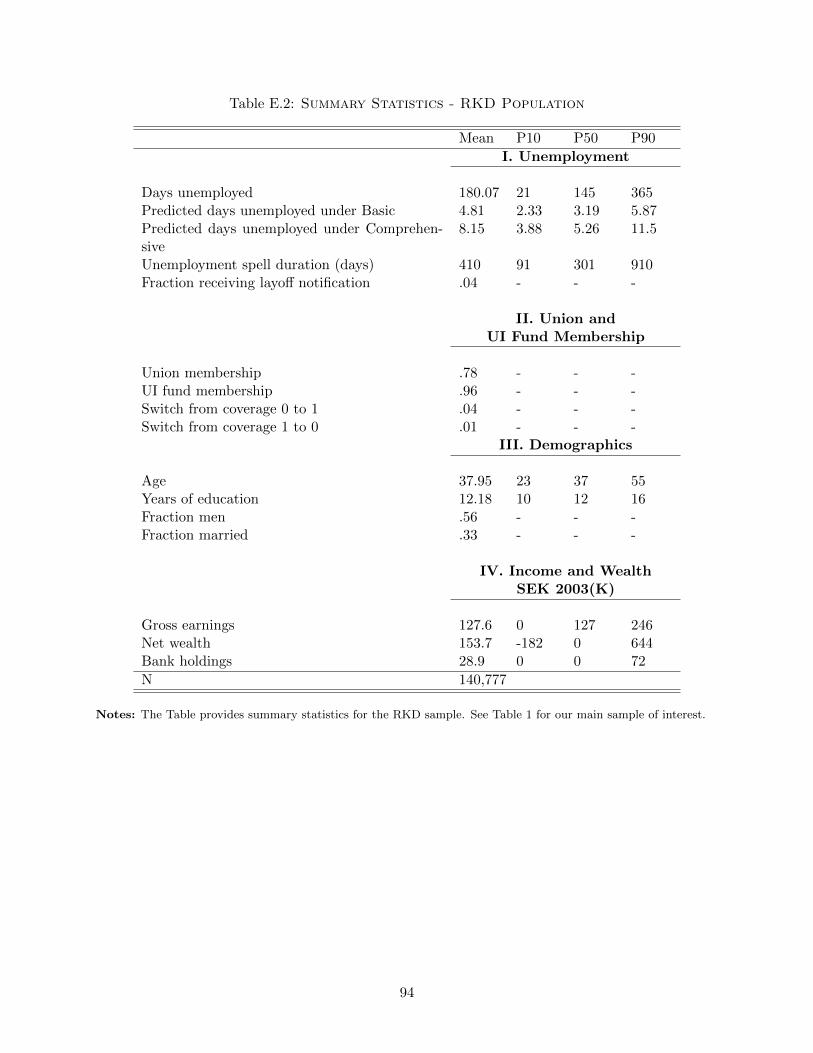
Table E.2: Summary Statistics - RKD Population

Mean P10 P50 P90

I. Unemployment

Days unemployed 180.07 21 145 365Predicted days unemployed under Basic 4.81 2.33 3.19 5.87Predicted days unemployed under Comprehen-sive

8.15 3.88 5.26 11.5

Unemployment spell duration (days) 410 91 301 910Fraction receiving layoff notification .04 - - -

II. Union andUI Fund Membership

Union membership .78 - - -UI fund membership .96 - - -Switch from coverage 0 to 1 .04 - - -Switch from coverage 1 to 0 .01 - - -

III. Demographics

Age 37.95 23 37 55Years of education 12.18 10 12 16Fraction men .56 - - -Fraction married .33 - - -

IV. Income and WealthSEK 2003(K)

Gross earnings 127.6 0 127 246Net wealth 153.7 -182 0 644Bank holdings 28.9 0 0 72

N 140,777

Notes: The Table provides summary statistics for the RKD sample. See Table 1 for our main sample of interest.

94

Appendix F Welfare Analysis: Additional Material

This appendix provides further detail and derivations for the theoretical analysis in Section 3 and

supporting material for the empirical implementation in Section 6.

F.1 Conceptual Framework: Further Details

To evaluate the design of the social insurance system allowing for choice, we characterized the

welfare impact of small changes in prices and coverages with two plan options, {(bj , pj)}j=1,0. This

relies on the social welfare function being concave and differentiable so that we can characterize

the optimal contract using first-order conditions. We also assumed that workers’ preferences are

quasi-linear in prices so that an individual’s risk πj , conditional on plan choice j, does not depend

on prices and neither does the ranking of individuals’ valuations ui. This is a standard assumption

in the insurance literature, but the implications from relaxing it are evident from the analysis of

coverage changes.

Regarding the timing of the model, we stick closely to the structure of the Swedish UI system

where individuals become eligible to receive the supplemental benefits when they have been con-

tributing for one year to the comprehensive coverage, and can opt in and out of the comprehensive

plan at any time. As a consequence, the value utj of plan j in year t depends on unemployment risk

πt+1, the expected number of days spent unemployed in year t + 1. With this in mind, we have

dropped time subscripts, but u (π) always refers to ut (πt+1), unless otherwise specified.

Our framework is highly stylized, but allows for multi-dimensional heterogeneity and endogenous

actions. Following a recent tradition in the social insurance literature [see Chetty and Finkelstein

[2013]], we choose not to explicitly model the underlying heterogeneity and actions. The key micro-

foundations for our analysis are the resulting plan valuations and costs and how they change with

the plans’ prices and coverage levels. For example, in a setting with expected utility and binary

unemployment risk, the value of a plan to a worker equals

ui (bj , pj) = maxa′

π(a′|θi

)u(bj − pj , a′|µi

)+(1− π

(a′|θi

))u(wi − pj , a′|µi

), (32)

while the insurer’s cost equals ci (bj , pj) = π(a′|θi)bj . The value and cost are interdependent

through the risk parameter θ and the effort choice a, which in turn depends on the preference

parameter µ that also affects the valuation. In general, a worker’s expected utility depends both on

the probability of job loss and the time spent unemployed. The government’s expected cost would

depend only on the expected number of days spent unemployed when the benefit profile is flat.

Sorting Effect The fiscal externality in both Propositions 1 and 2 depends on how many

individuals change in response to the policy (as captured by the demand elasticity) and the cost

characteristics of those who switch. We develop here formally why the cost characteristics of the

switchers in response to a change in coverage are different than for a change in price under multi-

95

dimensional heterogeneity.

We first re-write the social welfare function, ranking individuals based on their utility gain of

the comprehensive relative to the basic plan,

W ≡∫ui≥0

ω (ui (b1, p1)) di+

∫ui<0

ω (ui (b0, p0)) di+ λ {F1 [p1 − E1 (π1) b1] + F0 [p0 − E0 (π0) b0]} ,

=

∫u≥0

E(ω (u (b1, p1)) |u)dG (u) +

∫u<0

E(ω (u (b0, p0)) |u)dG (u)

+λ {(1−G (0)) [p1 − E1 (π1) b1] +G (0) [p0 − E0 (π0) b0]} .

Here G(·) is the distribution of u = u1 − u0, which depends on the plan characteristics, with

G(0) = F0 and 1 − G(0) = F1. Following the derivation in Veiga and Weyl [2016] and Handel et

al. [2019], we then find

∂

∂xj[(1−G (0))E1 (z1)] = E

z1

∂u∂xj

E(∂u∂xj|u = 0

) |u = 0

∂ (1−G (0))

∂xj. (33)

assuming no direct effect of the policy variable xj on the outcome z1.

The argument proceeds as following. First, using iterated expectations and introducing notation

u′ ≡ ∂u∂xj

, we can write

∂

∂xj[(1−G (0))E1 (z1)] =

∂

∂xj

[∫u≥0

E (z1|u) dG (u)

]=

∂

∂xj

[∫u≥0

∫E(z1|u,u′

)f(u′|u

)g (u) du′du

]=

∫∂

∂xj

[∫uε≥−u′×[xj−xε]

E(z1|uε,u′

)gε(uε|u′

)duε

]f(u′)du′

The last equality follows from (1) using f (u′|u) g (u) = g(u|u′

)f (u′), (2) approximating u (bj)∼= u (bε)+

u′ × [bj − bε], and substituting the variable in the integral u (bj)(≡ u) by u (bε)(≡ uε), where

du = duε, conditional on u′.

We can then apply Leibniz rule and find after re-substituting,

∂

∂xj

[∫u≥0

E (z1|u) dG (u)

]=

∫ [E(z1u′|u = 0,u′

)f(u′|u = 0

)du′]g (0)

= E

(z1∂u

∂xj|u = 0

)g (0) .

= E (z1|u = 0)E

(∂u

∂xj|u = 0

)g (0) + cov

(z1,

∂u

∂xj|u = 0

)

96

Note also that the effect on the share of individuals buying comprehensive coverage equals

∂ [1−G (0)]

∂xj=

∂

∂xj

[∫u≥0

dG (u)

]= E

(∂u

∂xj|u = 0

)g (0) .

Taken together, we can then indeed write

∂

∂xj[(1−G (0))E1 (z1)] = E

z1

∂u∂xj

E(∂u∂xj|u = 0

) |u = 0

∂ (1−G)

∂xj.

Similarly, we can find

∂

∂xj[G (0)E0 (z0)] = E

z0

∂u∂xj

E(∂u∂xj|u = 0

) |u = 0

∂G

∂xj

Applying this now to the difference in average risk for switchers in response to a coverage and

price change, we find

EM(bj)(πk)− EM(p)(πk) =cov

(πk,

∂uj∂bj|u = 0

)E(∂uj∂bj|u = 0

) .

Individuals with higher unemployment risk tend to value extra coverage more. However, with

heterogeneity in risk aversion (in addition to risk heterogeneity), the correlation between risks and

the marginal value of coverage among the marginal buyers can become negative [Ericson et al.

[Forthcoming]]. Relatedly, the risk-based selection into supplemental coverage may well worsen as

the basic coverage level increases. The reason is that the variation in willingness-to-pay coming

from heterogeneity in risk aversion, which would mute the risk-based selection, decreases as the

basic coverage becomes more generous [see Ericson et al. [Forthcoming]].

F.2 Proof of Proposition 1

We denote again by p and c, the difference in prices and costs between the two plans, e.g. p =

p1 − p0.

Proof. Differentiating the social welfare with respect to p0, we get:

∂W∂p0

= G (0)E0

(∂ω0

∂p0

)+ λ

{G (0)− ∂G (0)

∂p0p−∂ [(1−G (0))E1 (c1) +G (0)E0 (c0)]

∂p0

}.

Here, we are invoking the envelope theorem for the resorting of marginal individuals, ui (b1, p1) =

97

ui (b0, p0). We can rewrite this expression as

∂W∂p0

= G (0)E0

(∂ω0

∂p0

)+ λ

{G (0)− (p− EM (c))

∂G (0)

∂p0

}using the result in equation (33),

∂ [(1−G (0))E1 (c1) +G (0)E0 (c0)]

∂p0= EM (c1)

∂ [1−G (0)]

∂p0+ EM (c0)

∂G (0)

∂p0

= −EM (c)∂G (0)

∂p0.

Note that the quasi-linear assumption implies that prices do not cause any moral hazard response,

E0

(∂c0∂p0

)= E0

(b0∂π0∂p0

)= 0. Hence, the only impact on the budget constraint is the re-sorting

response. This response itself also simplifies due to the quasi-linearity assumption. Since ∂u∂p0

is constant, it depends on the demand response ∂G(0)∂p0

multiplied by the cost of providing the

supplemental coverage to workers at the margin, which simplifies to the unweighted average among

the marginals, EM (c) = E (c|u = 0). Using ∂G(0)∂p0

= −∂G(0)∂p , we then find that the FOC with

respect to the price of basic coverage, ∂W∂p0

= 0, is equivalent to

−E0

(∂ω0

∂p0

)= λ

{1 +ASp

∂ lnG (0)

∂p

}.

In a similar way, we can get the FOC for the price of the comprehensive plan

−E1

(∂ω1

∂p1

)= λ

{1 +ASp

∂ ln (1−G (0))

∂p

}Putting the two FOCs together, we get the expression in the Proposition.

F.3 Proof of Proposition 2

Proof. We consider the welfare impact of an increase in b0, for given prices and coverage b1. The

impact of a change in b0 on the government’s budget depends both on the change in selection into

both plans and the direct effect from increasing the coverage,

∂

∂b0

[∫u≥0

[p1 − E (c1|u)] dG (u) +

∫u<0

[p0 − E (c0|u)] dG (u)

]

=

p−E

c×∂u∂b0

E(∂u∂b0|u = 0

) |u = 0

∂(1−G (0))

∂b0−G (0)

∂E0c0

∂b0

≡ −[p−EM(b0) (c)

] ∂G (0)

∂b0−G (0)

∂E0c0

∂b0

98

By analogy to the subsidy change, we decompose the change in cost from providing coverage due to

the change in selection as the demand effect ∂G∂b0

multiplied by the fiscal externality p−EM(b0) (c),

caused by the switching of individuals who respond to the coverage change. This fiscal externality

differs from the fiscal externality of the subsidy as different individuals respond to a change in

coverage depending on their marginal value of basic coverage ∂u∂b0

, explaining the weights put on

the costs of the different marginals with u = 0. This is discussed in detail in Appendix F.1. In

addition to the selection response, an increase in coverage of the basic plan affects the government’s

expenditures directly, but also indirectly through a moral hazard response. That is,

∂E0c0

∂b0= E0 (π0) + E0

(∂π0

∂b0

)b0 = E0 (π0)

[1 + FEMH

b0

].

Invoking now the envelope condition for the individuals at the margin (i.e., u = 0), we find

dW = G (0)E0

(∂ω0

∂b0

)− λG (0)E0 (π0)

[1 + FEMH

b0

]− λ

[p− EM(b0) (c)

] ∂G∂b0

,

where

E0

(∂ω0

∂b0

)=

1

G (0)

∫u<0

E

(ω′ (u0)

∂u (b0, p0)

∂b0|u)dG (u)

Hence, at an (interior) optimum, we need dW =0 and thus

E0

(∂ω0

∂b0

)/E0 (π0) = λ

{1 + FEMH

b0 +[p− EM(b0) (c)

] ∂ lnG

∂b0/E0 (π0)

}.

In a similar way, we can get the FOC for the coverage of the comprehensive plan,

E1

(∂ω1

∂b1

)/E1 (π1) = λ

{1 + FEMH

b1 −[p− EM(b1) (c)

] ∂ ln (1−G)

∂b1/E1 (π1)

}.

Putting the two FOCs together, we get the expression in the Proposition.

99

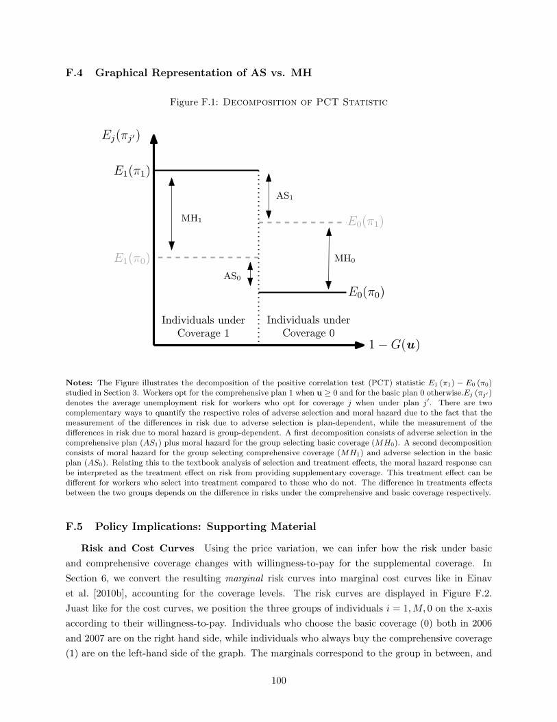
F.4 Graphical Representation of AS vs. MH

Figure F.1: Decomposition of PCT Statistic

Ej(πj′)

E1(π1)

MH1

E1(π0)

E0(π1)

MH0

AS0

E0(π0)

1−G(u)

Individuals under

Coverage 1

Individuals under

Coverage 0

AS1

Notes: The Figure illustrates the decomposition of the positive correlation test (PCT) statistic E1 (π1) − E0 (π0)studied in Section 3. Workers opt for the comprehensive plan 1 when u ≥ 0 and for the basic plan 0 otherwise.Ej (πj′)denotes the average unemployment risk for workers who opt for coverage j when under plan j′. There are twocomplementary ways to quantify the respective roles of adverse selection and moral hazard due to the fact that themeasurement of the differences in risk due to adverse selection is plan-dependent, while the measurement of thedifferences in risk due to moral hazard is group-dependent. A first decomposition consists of adverse selection in thecomprehensive plan (AS1) plus moral hazard for the group selecting basic coverage (MH0). A second decompositionconsists of moral hazard for the group selecting comprehensive coverage (MH1) and adverse selection in the basicplan (AS0). Relating this to the textbook analysis of selection and treatment effects, the moral hazard response canbe interpreted as the treatment effect on risk from providing supplementary coverage. This treatment effect can bedifferent for workers who select into treatment compared to those who do not. The difference in treatments effectsbetween the two groups depends on the difference in risks under the comprehensive and basic coverage respectively.

F.5 Policy Implications: Supporting Material

Risk and Cost Curves Using the price variation, we can infer how the risk under basic

and comprehensive coverage changes with willingness-to-pay for the supplemental coverage. In

Section 6, we convert the resulting marginal risk curves into marginal cost curves like in Einav

et al. [2010b], accounting for the coverage levels. The risk curves are displayed in Figure F.2.

Juast like for the cost curves, we position the three groups of individuals i = 1,M, 0 on the x-axis

according to their willingness-to-pay. Individuals who choose the basic coverage (0) both in 2006

and 2007 are on the right hand side, while individuals who always buy the comprehensive coverage

(1) are on the left-hand side of the graph. The marginals correspond to the group in between, and

100

their share is given in Figure 4, where we see the fraction of individuals buying dropping from 86

to 78% with the 2007 price increase. We plot with green dots the observed average realized risk,

measured by the number of days spent unemployed in year 2008, for the three groups. Note that

all risk measures in Figure F.2 are conditional on the vector of characteristics Z, and normalized

to the average risk under basic coverage of individuals observed under basic coverage E0 (π0). The

difference in realized risk (green dots) between the marginals and group 0 is therefore equivalent

to our semi-elasticity estimate SemiBaselineM(p) .

We then plot with blue triangles the average predicted risk under basic coverage and with red

triangles the average predicted risk under comprehensive coverage for all three groups. The blue

triangles identify the marginal risk curve in the basic coverage, while the red triangles plot the

marginal risk curve in the comprehensive coverage. These two curves provide all the information

necessary to compute the fiscal externality term FEASp that determines the optimal price level in

Proposition 1. Moreover, the difference between the red and blue triangles for each group identifies

the moral hazard of moving these individuals from basic to comprehensive coverage.

Consumption Smoothing Gains When considering to further differentiate the coverage

levels following Proposition 2, the fiscal externalities need to be traded off against the relative

consumption smoothing gains from extra coverages:E1

(∂ω1∂b1

)/E1(π1)

E0

(∂ω0∂b0

)/E0(π0)

. Given our estimates of the

fiscal externalities, further differentiation would therefore be socially valuable if the marginal utility

of an increase in benefits for individuals under the comprehensive coverage is worth at least 27%

more than the marginal utility of an increase in benefits for individuals under the basic coverage.

To estimate the magnitude of the relative consumption smoothing gains, we need to know

about the two basic forces that underlie them. The first is heterogeneity in the value of insurance,

conditional on risk: people who buy the comprehensive coverage may do so because they value an

additional kroner of consumption when unemployed more. Landais and Spinnewijn [Forthcoming]

find in the Swedish context that the mark-up workers under comprehensive coverage are willing

to pay for the supplemental coverage is 160% larger compared to workers under basic coverage,

conditional on their risk: E1(MRSb0,b1) = 2.6 ·E0(MRSb0,b1).51 This number underlines that there

is indeed significant heterogeneity in willingness-to-pay for insurance conditional on risk, which is

a strong force pushing for coverage differentiation.

The second force is diminishing marginal utility of consumption. The marginal utility of fur-

ther coverage should be estimated at coverage level b1 for individuals buying the comprehensive

coverage and at coverage level b0 for individuals in the basic plan. Diminishing marginal utility of

consumption makes the value of an additional kroner lower when evaluated at b1 than at b0.

Using a Taylor approximation, we can provide a back-of-the envelope calculation of the relative

consumption smoothing gains from extra coverage. We can indeed write that: Ej

(∂ωj∂bj

)/Ej (πj (bj)) ≡

51The mark-up MRSb0,b1 is defined as the average marginal rate of substitution between consumption whenemployed and unemployed evaluated between coverage level b0 and b1. These estimates come from the model ofTable 3 column (2), for which they find E1

(MRSb0,b1

)= 2.92, E0

(MRSb0,b1

)= 1.12

101

Figure F.2: Price Variation: Decomposition and Marginal Risk Curves

Group 1 Marginals Group 0

11.

52

2.5

33.

5U

nem

ploy

men

t Ris

k Ε i

(πi)

Rel

ativ

e to

Ε0(π

0)

.3 .4 .5 .6 .7 .8 .9 1Share Buying Comprehensive Insurance

Realized Risk (Days Unemployed)Predicted Days Under 0 Εi(π0)Predicted Days Under 1 Εi(π1)

Notes: The Figure uses estimates of Figure 5 to trace out the marginal risk curves under basic coverage andcomprehensive coverage using the sample of all eligible workers observed in 2006 and 2007. We start by positioningthe three groups of individuals j = 1,M, 0 on the x-axis according to their willingness-to-pay. Individuals whochoose the basic coverage (0) both in 2006 and 2007 are on the right hand side, while individuals who always buy thecomprehensive coverage (1) are on the left-hand side of the graph. The marginals correspond to the group in between,and their share is given in Figure 4, where we see the fraction of individuals buying dropping from 86 to 78% withthe 2007 price increase. We plot with green dots the observed average realized risk, measured by the number of daysspent unemployed in year t+1, for the three groups. All risk measures are conditional on the vector of characteristicsZ, and normalized to the average risk under basic coverage of individuals observed under basic coverage E0 (π0). Thedifference in realized risk (green dots) between the marginals and group 0 is therefore equivalent to our semi-elasticityestimate SemiBaselineM(p) . We then plot with blue triangles the average predicted risk under basic coverage and with redtriangles the average predicted risk under comprehensive coverage for all three groups. The blue triangles identify themarginal risk curve in the basic coverage, while the red triangles plot the marginal risk curve in the comprehensivecoverage. The difference between the red and blue triangles for each group identifies the moral hazard of movingthese individuals from coverage 0 to coverage 1. These two curves provide all the information necessary to computethe fiscal externality term FEASp that determines the optimal price level in Proposition 1.

102

Ej (u′ (cu (bj)) /u′ (ce (bj))) ∼= 1 + γ × Ej

(∆cc (bj)

), where cu and ce denote the consumption levels

when unemployed and employed, and γ = u′′(c)cu′(c) is the parameter of relative risk aversion. Sim-

ilarly, using a linear approximation for the mark-up, we have that: Ej(MRSb0,b1

) ∼= 1 + γ ×Ej(

∆cc (b0) + ∆c

c (b1))/2. This allows to link the average mark-up MRSb0,b1 estimated in Landais

and Spinnewijn [Forthcoming], to the marginal mark-ups evaluated at b0 and b1 respectively. In

practice, note that we unfortunately cannot observe the counterfactual consumption wedge between

employment and unemployment(

∆cc (bj)

)for workers when put under a different plan j. However,

we can easily provide bounds for these counterfactual drops. Assuming the consumption drop were

to double when changing from comprehensive to basic coverage (i.e. Ej(∆cc (b1)) = Ej(

∆cc (b0))/2),

we get a value of 1.97 for the left-hand side in Proposition 2. Note that Landais and Spinnewijn

[Forthcoming] find that the difference in consumption wedges for workers under comprehensive

and basic coverage is actually quite small.52 Assuming that the consumption drop doubles when

changing from comprehensive to basic coverage is therefore a conservative upper bound. In other

words, estimates from Landais and Spinnewijn [Forthcoming] suggest that the value of extra cov-

erage is likely much more than 27% larger for workers under comprehensive coverage compared to

workers under basic coverage, even when evaluated at b1 and b0 respectively. It follows that further

differentiation in coverage levels would probably enhance welfare.

52They indeed find that E0∆cc

(b0) = −.178(.25) and E1∆cc

(b1) = −.138(.036).

103