uniï¬ed constitutive modeling of rubber-like materials under
TRANSCRIPT

Unified constitutive modeling of rubber-like materials under diverse loadingconditions
Gerard-Philippe Zehila,∗, Henri P. Gavina
aDepartment of Civil and Environmental Engineering, Duke University, 121 Hudson Hall, Box 90287, Research Drive, Durham, NC 27708-0287,United States
Abstract
This paper presents a new constitutive model that unifies the behavioral characterizations of rubber-like materials ina broad range of loading regimes. The proposed model combines a selection of existing components that are knownto reflect, with suitable accuracy, two fundamental aspects of rubber behavior in finite strain: (i) rate-independentsoftening under deformation, also known as the Mullins effect, and (ii) hyper-viscoelasticity, including at high strainrates. The evolution model is further generalized to account for multiple rates of internal dissipation (or materialtime-scales). Suitable means of identifying the system’s parameters from simple uniaxial extension tests are explored.Several aspects of the model’s behavior are shown in virtual experiments of uniaxial extension, at different stretchrates. A possible directional approach extending the model to handle softening induced anisotropy is briefly discussed.
Keywords: Finite strain, nonlinear viscoelasticity, stress-softening, constitutive modeling, rubber-like materials.
1. Introduction and background
Several classes of models have been proposed to characterize the constitutive behavior of rubber-like materials(e.g. Boyce and Arruda, 2000). Micro-mechanical models are founded on the physics of polymer chain networks andstatistical methods (e.g. Arruda and Boyce, 1993; Drozdov and Dorfmann, 2004). Alternatively, phenomenologicalmodels rely on mathematical developments that are associated with conceptual representations or analogies with thepurpose of replicating the material’s behavior as observed at the macroscopic scale (e.g. Dorfmann and Ogden, 2004;Dorfmann and Pancheri, 2012; Gent, 1996; Hoo Fatt and Ouyang, 2007, 2008; Huber and Tsakmakis, 2000; Liu, 2010;Liu and Hoo Fatt, 2011; Ogden and Roxburgh, 1999; Pioletti et al., 1998). In some mixed approaches, constitutiveequations are founded on macroscopic models that contain statistical parameters reflecting a certain representation ofthe microscopic structure (e.g. D’Ambrosio et al., 2008; De Tommasi et al., 2006; Horgan et al., 2004).
Most existing material descriptions were developed under specific loading conditions. For instance, in the workof Brown (1997), the nonlinear dynamic behavior of filled elastomers is characterized at small strain amplitudes.Alternatively, Hoo Fatt and Ouyang (2008) propose a finite strain constitutive model for virgin Styrene Butadienerubber subjected to a high strain rate monotonic loading. Furthermore, Liu and Hoo Fatt (2011) present constitutiveequations, in finite strain, for the dynamic response of rubber under cyclic loading while D’Ambrosio et al. (2008),De Tommasi et al. (2006) and many others (e.g Chagnon et al., 2004, 2006; Dorfmann and Ogden, 2004; Dorfmannand Pancheri, 2012; Horgan et al., 2004; Marckmann et al., 2002; Ogden and Roxburgh, 1999) focus on character-izing main features of the rate independent softening behavior of elastomers, i.e. the Mullins effect (Mullins, 1969).Valuable reviews of the Mullins effect as well as of existing viscoelastic and hyperelastic constitutive laws were pro-vided by Diani et al. (2009), Boyce and Arruda (2000); Drapaca et al. (2007) and Marckmann and Verron (2006)respectively.
A careful inspection of the relevant literature furthermore reveals that a pertinent distinction can be made between:(i) models focusing on the rate independent softening behavior of the virgin material (e.g. D’Ambrosio et al., 2008;
∗Corresponding authorEmail address: [email protected] (Gerard-Philippe Zehil)
Preprint submitted to Elsevier July 16, 2013

De Tommasi et al., 2006), (ii) models describing its instantaneous response at high strain rates (e.g. Hoo Fatt andOuyang, 2007, 2008), and (iii) models relating the repeatable dynamic behavior of the non-virgin material undercyclic loading (e.g. Liu and Hoo Fatt, 2011).
However, in many applications, rubbers are exposed to diverse loading conditions acting on the material in differ-ent states. This is the case, for instance, of elastomeric structural bearings and expansion joints which are subjectedto prescribed displacements and tractions of various origins. While applied loads of increasing amplitude damage thepolymer chain network and cause material softening, intermittent unloading conditions associated with temperaturefluctuations can induce partial healing of the network and material stiffening by reentanglement and recross-linkingof the chains. At an appropriate time scale, part of the applied load is monotonic and, depending on the previousloading history, may be acting on a partially-healed polymeric network. Conversely, cyclic loads typically engage arepeatable behavior of the non-virgin material. Both monotonic and cyclic loads can be slowly varying thus gener-ating an equilibrium behavior (e.g. prescribed displacements due to material shrinking, creep, or thermal strains), orchange rapidly hence engaging an instantaneous and rate-dependent response (e.g. passing train, emergency breaking,accidental shock, wind gust, or earthquake).
When rubber-like materials are subjected to mechanical loading cycles, their hyper-viscoelastic response expe-riences stiffness and damping degradations. Alternatively, full or partial recovery of the material’s initial propertiescan occur following favorable changes in temperature and pressure. In many applications, the accurate predictionof such variations in the material’s behavior is of paramount importance in addressing system reliability as well ashuman safety issues. Failing to account for such changes in behavior, with sufficient accuracy, can result in tragic out-comes with potentially disastrous consequences. Unfortunately, existing constitutive models have a restrictive rangeof application and limited predictive ability. Because in engineering practice material characterizations are often usedunconnectedly while most viscoelastic models do not track the variations in the material’s behavior, current designsinvolving rate dependent responses tend to overlook the Mullins effect and therefore rely on inaccurate predictionsof the levels of degradation. This trend is further enhanced by the fact that, despite the abundance of tentative theo-ries, consensus has not yet been reached on the actual physical sources of the Mullins effect (e.g. Diani et al., 2009).Consequently, the softening of rubbers under first deformation is frequently eluded in practical applications and nodistinction is made between the primary response of the virgin material and its repeatable behavior under subsequentloadings.
In the current state of engineering practice, the prediction of a system’s response under combined loading regimes,engaging a rate-dependent response and a softening behavior simultaneously, requires combining separate materialmodels, each addressing a different aspect of material behavior. However, constitutive model libraries in commercialcodes are far from exhaustive. Model combination rules and modalities are also limited, sometimes poorly doc-umented and therefore opaque to the user. These facts often result in poorly-controlled modeling approximationswhich undermine prediction reliability and accuracy.
There are currently very few predictive models for the behavior of elastomers that also account for their degrada-tion and can therefore be considered as potential candidates to be used for the safe design of engineered components.Three-dimensional finite strain behavioral laws comprising hyperelastic, viscoelastic and elastoplastic componentswere proposed by Lin and Schomburg (2003), Lion (1996) and Miehe and Keck (2000). These formulations arebased on the theory of thermodynamics with internal state variables (Coleman and Gurtin, 1967) and retain differentchoices of such variables to characterize the evolution of internal dissipative processes. The Mullins stress-softeningeffect is assumed to act isotropically on all their components and it is accounted for within the framework of contin-uum damage mechanics (Kachanov, 1986; Lemaıtre, 1996) using a unique damage parameter. Despite their relativerheological completeness, these elaborate models continue to show notable imperfections in replicating true rubberbehavior: common shortcomings in modeling the Mullins effect are described for instance by Diani et al. (2009)while further predictive limitations can be directly seen upon comparing observed and fitted behaviors (e.g. Lin andSchomburg (2003, figure 8);Lion (1996, figures 2.1 and 4.1)). Clearly, more alternatives are needed as much remainsto be done in modeling elastomers.
2. Objective
In the absence of a unique and perfectly-accurate behavioral characterization of rubber-like materials, it is clearthat significant improvements in design efficiency as well as substantial reductions in engineering resources and com-
2
putational costs may be achieved by the provision of a greater number of unified formulations, valid under multipleloading conditions. Developing such models further would also contribute to reaching higher levels of accuracy byeliminating the need for approximate prediction combination techniques.
In order to address these goals, alternative constitutive formulations must be considered and their modeling capa-bilities explored. Building on the current state of knowledge in modeling elastomers, this paper puts forward a new,mixed, three-dimensional, constitutive description of rubbers, in finite strain. The proposed model is based on a care-ful selection of preexisting components accurately reflecting key rubber behavior in two different loading regimes: (i)the rate-independent softening under deformation, also known as the Mullins effect, and (ii) hyper-viscoelasticity, in-cluding high strain rates. This new model complements the set of existing mixed formulations and is believed to havea significant potential in meeting the aforementioned needs, particularly in applications involving those two regimes.
3. Proposed model
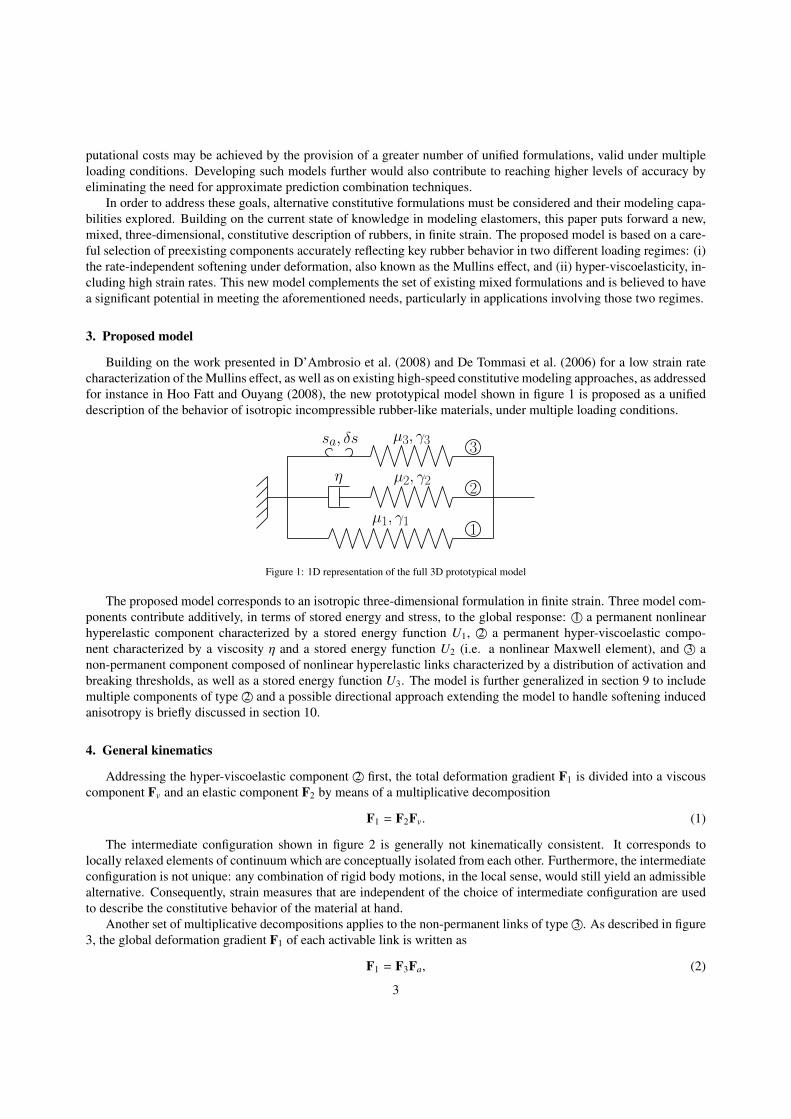
Building on the work presented in D’Ambrosio et al. (2008) and De Tommasi et al. (2006) for a low strain ratecharacterization of the Mullins effect, as well as on existing high-speed constitutive modeling approaches, as addressedfor instance in Hoo Fatt and Ouyang (2008), the new prototypical model shown in figure 1 is proposed as a unifieddescription of the behavior of isotropic incompressible rubber-like materials, under multiple loading conditions.
η
µ1, γ1
µ2, γ2
µ3, γ3sa, δs
1
2
3
Figure 1: 1D representation of the full 3D prototypical model
The proposed model corresponds to an isotropic three-dimensional formulation in finite strain. Three model com-ponents contribute additively, in terms of stored energy and stress, to the global response: 1© a permanent nonlinearhyperelastic component characterized by a stored energy function U1, 2© a permanent hyper-viscoelastic compo-nent characterized by a viscosity η and a stored energy function U2 (i.e. a nonlinear Maxwell element), and 3© anon-permanent component composed of nonlinear hyperelastic links characterized by a distribution of activation andbreaking thresholds, as well as a stored energy function U3. The model is further generalized in section 9 to includemultiple components of type 2© and a possible directional approach extending the model to handle softening inducedanisotropy is briefly discussed in section 10.
4. General kinematics
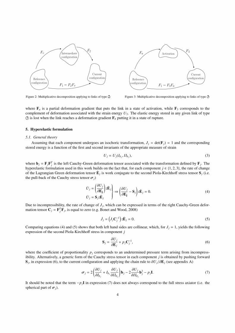
Addressing the hyper-viscoelastic component 2© first, the total deformation gradient F1 is divided into a viscouscomponent Fv and an elastic component F2 by means of a multiplicative decomposition
F1 = F2Fv. (1)
The intermediate configuration shown in figure 2 is generally not kinematically consistent. It corresponds tolocally relaxed elements of continuum which are conceptually isolated from each other. Furthermore, the intermediateconfiguration is not unique: any combination of rigid body motions, in the local sense, would still yield an admissiblealternative. Consequently, strain measures that are independent of the choice of intermediate configuration are usedto describe the constitutive behavior of the material at hand.
Another set of multiplicative decompositions applies to the non-permanent links of type 3©. As described in figure3, the global deformation gradient F1 of each activable link is written as
F1 = F3Fa, (2)
3
Referenceconfiguration
Intermediateconfiguration
Currentconfiguration
FvF2
F1 = F2Fv
Figure 2: Multiplicative decomposition applying to links of type 2©
Referenceconfiguration
Activation
Currentconfiguration
FaF3
F1 = F3Fa
Figure 3: Multiplicative decomposition applying to links of type 3©
where Fa is a partial deformation gradient that puts the link in a state of activation, while F3 corresponds to thecomplement of deformation associated with the strain energy U3. The elastic energy stored in any given link of type3© is lost when the link reaches a deformation gradient Fb putting it in a state of rupture.
5. Hyperelastic formulation
5.1. General theoryAssuming that each component undergoes an isochoric transformation, J j = det(F j) = 1 and the corresponding
stored energy is a function of the first and second invariants of the appropriate measure of strain
U j = U j(Ib j , IIb j ), (3)
where b j = F jFTj is the left Cauchy-Green deformation tensor associated with the transformation defined by F j. The
hyperelastic formulation used in this work builds on the fact that, for each component j ∈ {1, 2, 3}, the rate of changeof the Lagrangian Green deformation tensor E j is work conjugate to the second Piola-Kirchhoff stress tensor S j (i.e.the pull-back of the Cauchy stress tensor σ j)
U j =
(∂U j
∂Ej
):E j
U j = S j:E j
⇒(∂U j
∂Ej− S j
):E j = 0. (4)
Due to incompressibility, the rate of change of J j, which can be expressed in terms of the right Cauchy-Green defor-mation tensor C j = FT
j F j, is equal to zero (e.g. Bonet and Wood, 2008)
J j =(J jC−1
j
):E j = 0. (5)
Comparing equations (4) and (5) shows that both left hand sides are collinear, which, for J j = 1, yields the followingexpression of the second Piola-Kirchhoff stress in component j
S j =∂U j
∂E j+ p jC−1
j , (6)
where the coefficient of proportionality p j corresponds to an undetermined pressure term arising from incompress-ibility. Alternatively, a generic form of the Cauchy stress tensor in each component j is obtained by pushing forwardS j, in expression (6), to the current configuration and applying the chain rule to ∂U j/∂E j (see appendix A)
σ j = 2(∂U j
∂Ib j
+ Ib j
∂U j
∂IIb j
)b j − 2
∂U j
∂IIb j
b2j − p jI. (7)
It should be noted that the term −p jI in expression (7) does not always correspond to the full stress axiator (i.e. thespherical part of σ j).
4
5.2. Specialized formulationNumerous expressions of stored energy density functions are proposed in the literature (e.g. Marckmann and
Verron, 2006). The dependence of Ui on Ibi was found to be dominant in the case of incompressible rubber-likematerials (e.g. Yeoh, 1990). The following form will be retained for the purposes of this work
U j = µ j
(Ib j − 3
)γ j, (8)
where µ j and γ j are constant parameters, with j ∈ {1, 2, 3}. The underlying expression in (8) was reported capableof capturing the initially-stiff behavior of the material at high strain rates, without oscillating in the range of largedeformations by Hoo Fatt and Ouyang (2008). Substituting (8) into (7) yields the corresponding Cauchy stress ineach component
σ j = 2µ jγ j
(Ib j − 3
)γ j−1b j − p jI. (9)
6. Characterization of the non-permanent links
For simplicity, scalar activation and breaking criteria are retained for the non-permanent links: letting s(F1) be ascalar function of the global deformation gradient F1, each link is activated when s(F1) reaches its activation thresholdsa and breaks when s(F1) exceeds its breaking threshold sb ≥ sa. The active range of a non-permanent link is thereforecharacterized by the following expression
sa = s(F1 = Fa) ≤ s(F1) ≤ s(F1 = Fb) = sb, (10)
where Fa and Fb correspond to the values taken by F1 when s(F1) = sa and s(F1) = sb, respectively. Referring backto equation (2), the elastic deformation incurred by an active link is characterized by the partial deformation gradientF3 = F1F−1
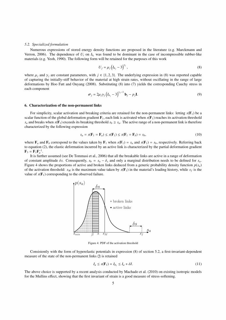
a .It is further assumed (see De Tommasi et al., 2006) that all the breakable links are active in a range of deformation
of constant amplitude δs. Consequently, sb = sa − δs and only a marginal distribution needs to be defined for sa.Figure 4 shows the proportions of active and broken links deduced from a generic probability density function p(sa)of the activation threshold: sM is the maximum value taken by s(F1) in the material’s loading history, while s f is thevalue of s(F1) corresponding to the observed failure.
sa
p(sa)
δs
sfsM
δs
s
broken links
active links
smin β
Figure 4: PDF of the activation threshold
Consistently with the form of hyperelastic potentials in expression (8) of section 5.2, a first-invariant-dependentmeasure of the state of the non-permanent links 3© is retained
Ia ≤ s(F1) = Ib1 ≤ Ia + δI. (11)
The above choice is supported by a recent analysis conducted by Machado et al. (2010) on existing isotropic modelsfor the Mullins effect, showing that the first invariant of strain is a good measure of stress-softening.
5

7. Global response
Components 1©, 2© and 3© of the proposed model (figure 1) contribute additively, in terms of internal energy andstress, to the global material response. The total stored energy density U and Cauchy stress σ are given by
U = U1 + U2 + U3, (12)σ = σ1 + σ2 + σ3. (13)
where U3 and σ3 correspond to the total contributions of the active links of type 3©, obtained following De Tommasiet al. (2006) by integration over the active range
[β, s
](see figure 4), with β = min{s,max{smin,max{s, sM} − δs}}, i.e.
U3 =
∫ s
β
U3 p(sa)dsa, (14)
σ3 =
∫ s
β
σ3 p(sa)dsa. (15)
8. Identification of model parameters
A feasible procedure is sought to determine the model parameters from simple uniaxial tension tests. In addition tothe unknown probability density function p(sa) of the activation threshold for the links of type 3©, relevant parametersare: η, δs, µ j and γ j for j ∈ {1, 2, 3}. In isochoric uniaxial tension, the generic deformation gradient F j writes
F j =
λ j 0 00 1√
λ j0
0 0 1√λ j
, (16)
where λ j is the principal stretch in the direction of the applied traction σ j. Substituting expression (16) into equation(9) and eliminating the pressure term p j yields the generic scalar expression for σ j
σ j = 2µ jγ j
(λ2
j −1λ j
) (Ib j − 3
)(γ j−1), (17)
where Ib j and λ j are in one to one correspondence, since Ib j = λ2j + 2/λ j increases monotonically with the stretch
λ j ≥ 1.
8.1. Low strain rate responseThe material’s quasi-static behavior is first examined in order to determine the parameters characterizing the dis-
tribution of activable links of type 3©. When deformation occurs at a sufficiently low strain rate, the hyper-viscoelasticcomponent 2© flows while remaining fully relaxed. As shown in figure 5, the conceptual representation correspondingto this case reduces to branches 1© and 3© of the prototypical model.
µ1, γ1
µ3, γ3sa, δs
1
3
Figure 5: Reduced model at low strain rate
To simplify notations, let λ = λ1 and I(λ) = Ib1 (λ). A virgin dumbbell-shaped sample of rubber is loaded andunloaded, at a sufficiently low constant strain rate, up to increasing values of the maximum stretch λM correspondingto IM = I(λM). This may be done following the increasing triangular strain-history profile shown in figure 11(a) while
6
I(λ)
σ(I)
primary loading path
I∗MIMδI
Figure 6: δI corresponds to the global elastic range of the virginmaterial
λ
σ(λ)
primary loading curve
generic path
σ1(λ) + σ3(λ)
σ1(λ)
λM
σ3(λ)
Figure 7: Illustration of material softening at low strain rate: σ(λ) =
σ1(λ) + σ3(λ)
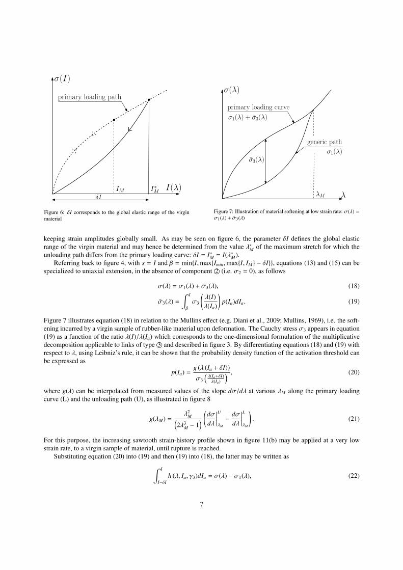
keeping strain amplitudes globally small. As may be seen on figure 6, the parameter δI defines the global elasticrange of the virgin material and may hence be determined from the value λ∗M of the maximum stretch for which theunloading path differs from the primary loading curve: δI = I∗M = I(λ∗M).
Referring back to figure 4, with s = I and β = min{I,max{Imin,max{I, IM} − δI}}, equations (13) and (15) can bespecialized to uniaxial extension, in the absence of component 2© (i.e. σ2 = 0), as follows
σ(λ) = σ1(λ) + σ3(λ), (18)
σ3(λ) =
∫ I
β
σ3
(λ(I)λ(Ia)
)p(Ia)dIa. (19)
Figure 7 illustrates equation (18) in relation to the Mullins effect (e.g. Diani et al., 2009; Mullins, 1969), i.e. the soft-ening incurred by a virgin sample of rubber-like material upon deformation. The Cauchy stress σ3 appears in equation(19) as a function of the ratio λ(I)/λ(Ia) which corresponds to the one-dimensional formulation of the multiplicativedecomposition applicable to links of type 3© and described in figure 3. By differentiating equations (18) and (19) withrespect to λ, using Leibniz’s rule, it can be shown that the probability density function of the activation threshold canbe expressed as
p(Ia) =g (λ (Ia + δI))
σ3
(λ(Ia+δI)λ(Ia)
) , (20)
where g(λ) can be interpolated from measured values of the slope dσ/dλ at various λM along the primary loadingcurve (L) and the unloading path (U), as illustrated in figure 8
g(λM) =λ2
M(2λ3
M − 1) (
dσdλ
∣∣∣∣∣UλM
−dσdλ
∣∣∣∣∣LλM
). (21)
For this purpose, the increasing sawtooth strain-history profile shown in figure 11(b) may be applied at a very lowstrain rate, to a virgin sample of material, until rupture is reached.
Substituting equation (20) into (19) and then (19) into (18), the latter may be written as∫ I
I−δIh (λ, Ia, γ3)dIa = σ(λ) − σ1(λ), (22)
7

λ
σ(λ)primary loading curve
λM1 λM2 λMiλMn
(L)
(U1)
dσdλ
∣∣∣∣L
λM1
(U2)
(Ui)
(Un)
dσdλ
∣∣∣∣U1
λM1
dσdλ
∣∣∣∣L
λM2
dσdλ
∣∣∣∣U2
λM2
dσdλ
∣∣∣∣L
λMi
dσdλ
∣∣∣∣Ui
λMi
dσdλ
∣∣∣∣L
λMn
dσdλ
∣∣∣∣Un
λMn
Figure 8: Determining data points(λMi , g
(λMi
))
where the quantity on the right-hand-side can be deduced from the measured data (see figure 7). The parameter µ3simplifies in the expression of h (λ, Ia, γ3), which is given by the ratio
h (λ, Ia, γ3)g (λ (Ia + δI))
=σ3
(λ(I)λ(Ia)
)σ3
(λ(Ia+δI)λ(Ia)
) . (23)
The parameter γ3 can be obtained from equation (22) by prediction error minimization. Once γ3 is known, equation(20) can be normalized such that
∫ I f−δIImin
p(Ia)dIa = 1 which yields the parameter µ3.It may hence be concluded that all the parameters characterizing the distribution of activable links of type 3©,
including the probability density function of their activation threshold, can be determined by performing a multistageuniaxial tension test, at low strain rate, on a sample of virgin rubber. It remains to determine the parameters governingthe behavior of the links of type 1© and 2©, which is precisely the goal of the following section.
8.2. Repeatable responseIn this section, we consider the constitutive behavior of the non-virgin material in a range of deformation such
that all remaining non-permanent links of type 3© are kept below their activation threshold. As shown in figure 9 theconceptual representation corresponding to this case reduces to branches 1© and 2© of the prototypical model.
η
µ1, γ1
µ2, γ2
1
2
Figure 9: Reduced model in the repeatable range
8.2.1. Nonlinear hyper-viscoelastic formulationWith j ∈ {1, 2, v}, let C j = FT
j F j and b j = F jFTj be right and left Cauchy-Green deformation tensors and denote by
E j and e j the corresponding Green and Almansi strain tensors, respectively. Furthermore, let T and Γ be intermediatemeasures of the global stress and strain, i.e.
T = FvSFTv = F−1
2 σF−T2 , (24)
Γ = F−Tv E1F−1
v = FT2 e1F2. (25)
8

The tensors S and σ in expression (24) correspond to measures of the global stress in the reference and currentconfigurations respectively. Alternatively, Γ may be written as
Γ =12
(FT
2 F2 − I)
+12
(I − F−T
v F−1v
)= E2 + ev, (26)
where E2 and ev are seen as intermediate measures of strain associated with the hyperelastic and viscous parts ofcomponent 2©, respectively. Differentiating (26) with respect to time yields the relationship between the correspondingstrain rates
Γ = E2 + ev. (27)
The Lie derivative Γ of Γ corresponds to the push-forward of E1 to the intermediate frame, i.e.
Γ , F−Tv E1F−1
v = Γ + lTv Γ + Γlv, (28)
where lv is the velocity gradient in the intermediate system of coordinates xv, i.e.
lv ,∂v∂xv
= FvF−1v . (29)
Let Dint be the internal power dissipation due to the viscous effects. The second law of thermodynamics may beexpressed pointwise, in the reference frame, by means of the Clausius-Planck inequality (e.g. Holzapfel, 2000)
Dint = S:E1 − U − SΘ ≥ 0, (30)
where S is the entropy density, Θ denotes the rate of change in temperature and U corresponds to the rate of changein free energy density. Assuming a constant temperature, inequality (30) specializes into
Dint = S:E1 − U ≥ 0. (31)
Expression (31) may be pushed forward to the intermediate frame as
T:Γ − U ≥ 0. (32)
The total Helmholtz free energy density U is then written as the sum of the energy densities stored in the hyperelasticportions of components 1© and 2©, each depending on the appropriate measure of strain
U = U1(E1) + U2(E2). (33)
The rates of change of U1 and U2 may now be expressed as follows
U1 =∂U1
∂E1:E1, (34)
U2 =∂U2
∂E2:E2. (35)
Inverting equation (28) for E1 and substituting into equation (34) yields the rate of change in U1 as
U1 =
(Fv∂U1
∂E1FT
v
):Γ. (36)
On the other hand, manipulating equations (27) and (28) it can be shown that E2 satisfies
E2 = Γ − dv − lTv E2 − E2lv, (37)
where dv is the rate of deformation of the viscous component in 2©
dv =12
(lv + lTv
)= ev + lTv ev + evlv. (38)
9

Comparing the right-hand-sides of expressions (28) and (38) shows that dv is the Lie derivative of ev. Pluggingequation (38) into (37) and then (37) into (35) yields the rate of change in U2 as
U2 =∂U2
∂E2:Γ −
(C2
∂U2
∂E2
):dv, (39)
where, in the case of an isotropic material, the Mendel stress (C2∂U2/∂E2) is symmetric. Defining intermediatemeasures of partial stress in components 1© and 2© respectively as
T1 = Fv∂U1
∂E1FT
v and T2 =∂U2
∂E2, (40)
then substituting equation (36) and (39) into (32) yields the following inequality (e.g. Hoo Fatt and Ouyang, 2008;Huber and Tsakmakis, 2000)
Dint = [T − (T1 + T2)] :Γ + [C2T2] :dv ≥ 0, (41)
where the history of the global deformation gradient F1, and hence the tensorial quantity Γ, can be chosen arbitrarily.A standard procedure due to Coleman and Noll (1963); Coleman and Gurtin (1967) is applied to satisfy inequality(41):
• In the particular case where the rate of deformation of the viscous component is equal to zero (i.e. dv = 0), thetransformation process is reversible and inequality (41) reduces to
Dint = [T − (T1 + T2)] :Γ = 0. (42)
Equality (42) is satisfied for every choice of F1 if and only if
T = T1 + T2 ⇐⇒ σ = σ1 + σ2. (43)
• Assuming that local equilibrium (43) is satisfied in the general case where dv , 0, expression (41) reduces to
(C2T2) :dv ≥ 0. (44)
It is noteworthy that inequality (44) is independent of the choice of intermediate configuration. For an isotropicmaterial, the “Mandel” stress tensor C2T2 is symmetric. The following evolution law was proposed by Huber andTsakmakis (2000) as a simple condition that satisfies inequality (44)
dv =1η
(C2T2)d , (45)
where the superscript (.)d denotes a deviatoric component. Using (45) and denoting the velocity gradients by l j =
F jF−1j , it can be shown that
b2 = l1b2 + b2lT1 −2η
b2σd2. (46)
8.2.2. Practical subsystem identification (saturation method)Following a procedure proposed by Hoo Fatt and Ouyang (2008), the parameters µ1 and γ1 can be determined first
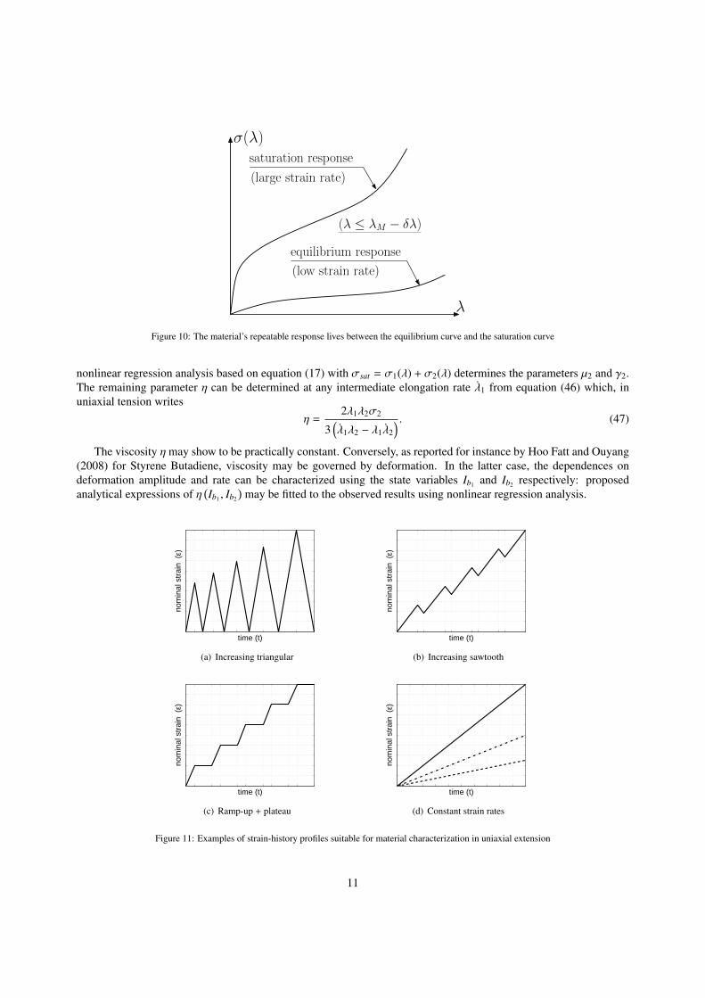
by a nonlinear regression analysis based on equation (17) with j = 1. The corresponding equilibrium response σ1 (seefigure 10) is obtained by loading a non-virgin material sample in uniaxial extension at a suitably low constant strainrate (ramp-up) and holding it at increasing values of constant strain (plateau) to allow for relaxation of the overstressσ2 in component 2©. This combined constant strain rate and incremental stress relaxation test is illustrated in figure11(c). Intervals of constant strain must be adjusted according to the material’s relaxation spectrum.
The subsystem in figure 9 may be further identified using monotonic strain-history profiles of (preferably) constantstrain rates (see figure 11(d)). Subjecting the sample to a sufficiently high strain rate will induce locking of the viscouscomponent (i.e. λv = 0) and yield the saturation response σsat (see figure 10) corresponding to λ1 = λ2 = λ. A
10
λ
σ(λ)saturation response
(large strain rate)
equilibrium response
(low strain rate)
(λ ≤ λM − δλ)
Figure 10: The material’s repeatable response lives between the equilibrium curve and the saturation curve
nonlinear regression analysis based on equation (17) with σsat = σ1(λ) + σ2(λ) determines the parameters µ2 and γ2.The remaining parameter η can be determined at any intermediate elongation rate λ1 from equation (46) which, inuniaxial tension writes
η =2λ1λ2σ2
3(λ1λ2 − λ1λ2
) . (47)
The viscosity η may show to be practically constant. Conversely, as reported for instance by Hoo Fatt and Ouyang(2008) for Styrene Butadiene, viscosity may be governed by deformation. In the latter case, the dependences ondeformation amplitude and rate can be characterized using the state variables Ib1 and Ib2 respectively: proposedanalytical expressions of η
(Ib1 , Ib2
)may be fitted to the observed results using nonlinear regression analysis.
time (t)
nom
inal
str
ain
(ε)
(a) Increasing triangular
time (t)
nom
inal
str
ain
(ε)
(b) Increasing sawtooth
time (t)
nom
inal
str
ain
(ε)
(c) Ramp-up + plateau
time (t)
nom
inal
str
ain
(ε)
(d) Constant strain rates
Figure 11: Examples of strain-history profiles suitable for material characterization in uniaxial extension
11

8.2.3. Practical subsystem identification (PEM method)The methodology described in section 8.2.2 relies on an ability to achieve sufficiently high (constant) strain rates,
in order to provoke saturation of the viscous component. Practically obtainable rates using commercially availableservohydraulic test machines are limited. Higher rates in traction can be acheived with specifically-designed testingapparatus like the modified Charpy impact machine described by Hoo Fatt and Ouyang (2008) or the falling weightapparatus proposed by Roland (2006).
In case technical difficulties are encountered in this regard, one alternative approach would be to determine theparameters of components 1© and 2© simultaneously, by prediction error minimization (PEM) with respect to therepeatable behavior, as observed within the range of achievable strain rates. Indeed, expressions for the overstress σ2resulting from equations (17) and (47) may be equated to obtain a nonlinear ordinary differential equation (ODE) inthe elastic component of the stretch λ2(t) in branch 2©. For the purpose of numerical computations, a convenient ODEformulation is obtained in terms of the proxy variable y = λ1/λ2, i.e.
dydt
=2y3ησ2
(λ1
y
). (48)
Given a global stretch history λ1(t) = λ(t), the aforementioned ODE can be solved for λ2(t) using current iteratesfor the model’s parameters. The predicted history of the total stress σ(t) is obtained by adding its two componentsevaluated using expressions ((17) with j ∈ {1, 2}) and compared, at each iteration, to the observed response.
9. Generalized model
The prototypical model shown in figure 1 can be generalized further to include a number n ≥ 1 of nonlinear hyper-viscoelastic Maxwell elements of type 2©. The procedure described in section 8.1 for characterizing the low strain rateresponse remains unchanged. However, for n > 1, the saturation method of section 8.2.2 cannot be applied to identifythe repeatable behavior. A generalized version of the alternative method based on prediction error minimization (seesection 8.2.3) may be used instead.
The ith type 2©Maxwell element (1 ≤ i ≤ n) is characterized by a viscosity ηi and a free energy density U2,i. It isfurther associated with a proper intermediate configuration Ii and the corresponding multiplicative decomposition
F1 = F2,iFv,i. (49)
Following a similar derivation to the one presented in section 8.2.1, it can be shown that inequality (41) generalizesinto a set of n equivalent inequalities of the formTi −
Ti1 +
n∑j=1
Ti2, j
:Γi +
n∑j=1
(C2, jT j
2, j
):dv, j ≥ 0, (50)
where the partial stress Ti2, j in the jth hyperelastic component and the total stress Ti are expressed in Ii. The quantity
Γi corresponds to the Lie derivative of the ith intermediate measure of global strain and dv, j denotes the rate ofdeformation of the jth viscous component, expressed in I j. Following the Coleman-Noll procedure, expression (50)reveals the general additivity of partial stresses, i.e.
Ti = Ti1 +
n∑j=1
Ti2, j (∀ j) ⇐⇒ σ = σ1 +
n∑j=1
σ2, j, (51)
as well as a generalized dissipation inequality:
Dint =
n∑j=1
(C2, jT j
2, j
):dv, j ≥ 0. (52)
12

Inequality (52) can be satisfied simply, by retaining for the n viscous components, uncoupled evolution laws of theform given by expression (45), i.e.
dv, j =1η j
(C2, jT j
2, j
)d. (53)
Using the laws in (53), expressions (46), (47) and (48) can be generalized to the jth component of type 2© as follows
b2, j = l1b2, j + b2, jlT1 −2η j
b2, jσd2, j, (54)
η j =2λ1λ2, jσ2, j
3(λ1λ2, j − λ1λ2, j
) , (55)
dy j
dt=
2y j
3η jσ2, j
(λ1
y j
). (56)
In a stretch-driven uniaxial extension test, the global stretch history λ1(t) = λ(t) is known. Assuming an initial guessfor the parameters characterizing component 1© and the components of type 2©, the n uncoupled ODE’s given byexpression (56) can be solved for the elastic portions λ2,i(t) of the stretch in each Maxwell element. The partialstress in each hyperelastic component can be determined from its constitutive equation, i.e. equation (17) in thepresent case. A predicted history of the total stress σ(t) is obtained by summation according to expression (51). Thedifference between the predicted response and the observed response can be minimized by iterating on the model’sparameters.
10. Mullins effect induced anisotropy
10.1. A brief overview
Based on considerations of material symmetry, but also on the implicit assumption of a directional network alter-ation (as opposed to an isotropic one), Horgan et al. (2004) argue that the damage associated with the Mullins effectis inherently anisotropic and briefly discuss a tensorial approach to account for this anisotropy. Experimental data(e.g. Dargazany and Itskov, 2009; Diani et al., 2006; Dorfmann and Pancheri, 2012; Itskov et al., 2006; Machadoet al., 2012) confirm that stress softening introduces some anisotropy in the material response. Diani et al. (2006) andDargazany and Itskov (2009) present micromechanical directional models to handle softening induced anisotropy. Thepotential of several finite-directional models in reflecting the behavioral anisotropy induced by the Mullins effect ininitially isotropic hyperelastic materials is tested by Gillibert et al. (2010), based on the models’ initial anisotropy andtheir ability to replicate the behavior of a full (i.e. infinite-directional) network. Dorfmann and Pancheri (2012) buildon the tensorial approach outlined by Horgan et al. (2004) and derive a simple phenomenological model accountingfor stress softening and changes in material symmetry. The model applies, in its current form, to pure homogeneousdeformations; however, it may be extended to more general loading conditions by the addition of an evolution law.
10.2. Outline of model extension
The formulation characterizing component 3© of the mixed model presented in this paper can also be extended,in several ways, to handle softening induced anisotropy. A possible directional approach, preserving the form ofstored energy density given by equation (8), with j = 3, as well as the scalar measure of the active range specified inexpression (11), is outlined hereafter.
To this end, component 3© can be considered as a collection of incompressible directional networks. Each networkN (u) has an elongated shape; it is oriented in a given direction of unit vector u and comprises a very large numberof activable/breakable links characterized by a distribution of activation thresholds similar to the one illustrated onfigure 4. It is further assumed that, under the global deformation gradient F = F1, each directional network N (u) ofcomponent 3© softens isotropically while subjected to a uniaxial deformation characterized by the stretch λ(u) resultingfrom F in direction u, i.e.
λ(u) =√
(Fu) . (Fu) =√
uT Cu, (57)
13

where C = FT F. Under these conditions, the scalar measure of deformation of network N (u) is given by the quantityI(u) = λ(u)2
+ 2/λ(u). As is usually the case in directional models, the number of spatial directionsN (u) can be finite orinfinite. An infinite-directional formulation is outlined below in analytical form, which can be numerically integratedon the surface of a unit sphere, for instance, using sets of collocation directions and weights determined by Bazantand Oh (1986).
The stored energy density and the principal Cauchy stress in the direction of the current unit vector Fu/λ(u),associated with an active link of network N (u), are given by
U(u)3 = µ3
(I(u)3 − 3
)γ3= µ3
λ(u)3
2+
2
λ(u)3
− 3
γ3
, (58)
σ(u)3 = λ(u)
3
dU(u)3
dλ(u)3
+ p(u)3 = 2
λ(u)3
2−
1
λ(u)3
dU(u)3
dI(u)3
+ p(u)3 , (59)
where p(u)3 is an undetermined pressure term arising from incompressibility. All active links in a given directional
networkN (u) contribute additively, in terms of stored energy density and stress, to the elastic response of the network.The latter is hence found by summation over the active range, i.e.
U(u)3 =
∫ I(u)3
β(u)U(u)
3 p(Ia)dIa, (60)
σ(u)3 =
1
λ(u)2
∫ I(u)3
β(u)σ(u)
3 p(Ia)dIa (Fu) ⊗ (Fu). (61)
Expressions for the total elastic response of component 3© are finally obtained by integrating equations (60) and (61)on the surface of a unit sphere S
U3 =1
4π
∫S
∫ I(u)3
β(u)U(u)
3 p(Ia)dIa
dS(u), (62)
σ3 = 2F
14π
∫S
∫ I(u)3
β(u)
1 − 1
λ(u)3
3
dU(u)3
dI(u)3
p(Ia)λ (Ia)2 dIa u ⊗ u
dS(u)
FT + p3I. (63)
Assuming a suitable analytical expression for p(Ia) in terms of parameters, the anisotropic stress response ofcomponent 3© to a given global deformation history F(t) can be predicted using equation (63). Consequently, themodel’s parameters can be fitted to experimental data by minimizing the prediction error.
11. Example
Referring to figure 1, with a single component of type 2©, the following set of numerical parameters is chosen toillustrate some aspects of the isotropic model’s behavior in uniaxial extension at different strain rates: µ1 = 1.1 MPa,γ1 = 0.8, µ2 = 3.3 MPa, γ2 = 1.1, µ3 = 19.8 MPa, γ3 = 0.7, η = 0.05 MPa.s and δI = 5. The activation threshold Ia
of the first invariant of global strain is taken to follow the probability density function of a beta distribution, which isbounded (see e.g. Ang and Tang, 2007), i.e.
p(Ia) =1
β(p, q)(Ia − Ia,min)p−1(Ia,max − Ia)q−1(
Ia,max − Ia,min)p+q−1 , (64)
where Ia ∈[Ia,min, Ia,max
]with Ia,min = 3 and Ia,max =
(I f − δI
)= 100. The standard beta function appearing in the
denominator of expression (64) is given by
β(p, q) =
∫ 1
0xp−1(1 − x)q−1dx. (65)
14

3 10 20 30 40 50 60 70 80 90 1000
0.01
0.02
0.03
0.04
0.05
Probability Density Function of Activation Threshold
activation threshold Ia
prob
abili
ty p
(Ia)
p(Ia) → β distribution
Figure 12: Assumed probability density function of the activationthreshold Ia characterizing the links of type 3©: p (Ia) follows a β-distribution with p = 3, q = 13 and Ia ∈ [1, 100].
0 4 8 14 20 28 361
1.5
2
2.5
3
3.5
4
4.5
5Normalized History of Applied Global Stretch
stretch rate × time
glob
al s
tret
ch λ
λλ
max
Figure 13: Virgin models are subjected, in uniaxial extension, to astandardized history of global stretch at different stretch rates: λ1 =
0.1 s−1, 200 s−1 and 600 s−1.
Figure 12 shows the probability density function of Ia for p = 2 and q = 13, which is positively skewed.The three-component model is subjected, uniaxially, to the normalized history of global stretch defined in figure
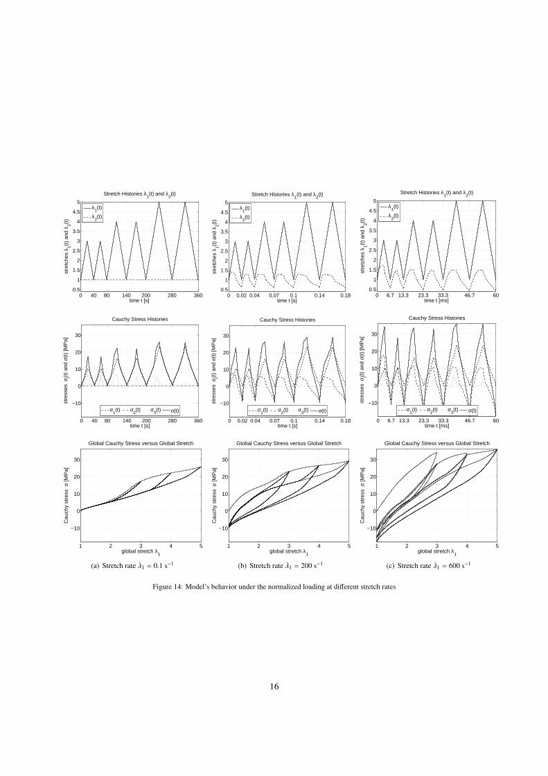
13: three sets of two stretch-driven loading cycles are applied to the virgin model, at increasing stretch amplitudesλM = 3, 4 and 5. This virtual experiment is repeated at three different stretch rates λ1 = 0.1 s−1, 200 s−1 and 600 s−1.
The model’s response to the lowest stretch rate λ1 = 0.1 s−1 can be seen on the set of figures 14(a). At this rate, thevirtual experiment is performed sufficiently slowly, with respect to the material’s internal time-scale, for the viscoussubcomponent to flow at nearly the same rate and undertake most of the applied stretch. Consequently, the elasticsubcomponent of element 2© remains unloaded with λ2 ≈ 0 and σ2 ≈ 0. On the other hand, the history of the stress incomponent 3© is consistent with the deterioration process to which the corresponding links are subjected to. It can benoted for instance that, over each set (i) of two successive loading cycles of same stretch amplitude λMi , σ3(t) has aweaker intensity preceding the instant at which the maximum applied stretch λMi occurs, and that it follows the samepattern past that point. When subjected to a sufficiently low rate of stretch, the system behaves as the reduced modelshown in figure 5 and hence undergoes a pure Mullins effect.
The sets of figures 14(b) and 14(c) show the model’s behavior at higher stretch rates: λ1 = 200 s−1 and 600s−1 respectively. The responses of components 1© and 3© in a stretch-driven experiment are clearly rate-independent.Element 2© however, behaves differently: the internal rate of dissipation of its viscous subcomponent being limited,the elastic subcomponent, which responds instantaneously, undertakes larger parts λ2 of the applied stretch λ1, atlarger stretch rates. Upon unloading, and despite a state of global extension with λ1 ≥ 1, the delayed viscous responseresults in the compression of component 2© with λ2 ≤ 1 and σ2 ≤ 0.
Further, it is interesting to note that, at sufficiently high strain rates, the peak in total stress σ(t) drops significantlybetween the first and the second loading cycles. In the present case, this is less apparent in subsequent sets of largerglobal stretch amplitude. However, the magnitude of such drops can be modulated by changing the stretch rate orintroducing time delays between successive loading sets. This phenomenon is clearly a manifestation of the model’sviscoelastic behavior and should not be mistaken with stress-softening or damage.
12. Conclusions
A new three-dimensional multi-regime evolution model for rubber-like materials is presented in this work. Theproposed model is based on a selection of existing components and unifies two major aspects of rubber behavior, inlarge deformations: nonlinear viscoelasticity and the Mullins effect. The prototypical formulation is further general-ized to include multiple nonlinear Maxwell elements accounting for several internal material time-scales. A detailedanalysis provides practical means of determining the model’s parameters from simple uniaxial extension tests. Anumerical example illustrates several aspects of the model’s behavior in uniaxial extension, at different stretch rates.A possible directional approach extending the model to handle Mullins effect induced anisotropy is briefly discussed.
15
0 40 80 140 200 280 3600.5
1
1.5
2
2.5
3
3.5
4
4.5
5
Stretch Histories λ1(t) and λ
2(t)
time t [s]
stre
tche
s λ 1(t
) an
d λ 2(t
)
λ1(t)
λ2(t)
0 0.02 0.04 0.07 0.1 0.14 0.180.5
1
1.5
2
2.5
3
3.5
4
4.5
5
Stretch Histories λ1(t) and λ
2(t)
time t [s]
stre
tche
s λ 1(t
) an
d λ 2(t
)
λ1(t)
λ2(t)
0 6.7 13.3 23.3 33.3 46.7 600.5
1
1.5
2
2.5
3
3.5
4
4.5
5
Stretch Histories λ1(t) and λ
2(t)
time t [ms]
stre
tche
s λ 1(t
) an
d λ 2(t
)
λ1(t)
λ2(t)
0 40 80 140 200 280 360
−10
0
10
20
30
Cauchy Stress Histories
time t [s]
stre
sses
σi(t
) an
d σ(
t) [M
Pa]
σ1(t) σ
2(t) σ
3(t) σ(t)
0 0.02 0.04 0.07 0.1 0.14 0.18
−10
0
10
20
30
Cauchy Stress Histories
time t [s]
stre
sses
σi(t
) an
d σ(
t) [M
Pa]
σ1(t) σ
2(t) σ
3(t) σ(t)
0 6.7 13.3 23.3 33.3 46.7 60
−10
0
10
20
30
Cauchy Stress Histories
time t [ms]
stre
sses
σi(t
) an
d σ(
t) [M
Pa]
σ1(t) σ
2(t) σ
3(t) σ(t)
1 2 3 4 5
−10
0
10
20
30
Global Cauchy Stress versus Global Stretch
global stretch λ1
Cau
chy
stre
ss σ
[MP
a]
(a) Stretch rate λ1 = 0.1 s−1
1 2 3 4 5
−10
0
10
20
30
Global Cauchy Stress versus Global Stretch
global stretch λ1
Cau
chy
stre
ss σ
[MP
a]
(b) Stretch rate λ1 = 200 s−1
1 2 3 4 5
−10
0
10
20
30
Global Cauchy Stress versus Global Stretch
global stretch λ1
Cau
chy
stre
ss σ
[MP
a]
(c) Stretch rate λ1 = 600 s−1
Figure 14: Model’s behavior under the normalized loading at different stretch rates
16

Appendix A
Intermediate steps between equations (6) and (7) are detailed hereafter: equation (6) is pushed forward to thecurrent configuration, in the usual way, to yield
σ j = F j∂U j
∂E jFT
j + p jI. (66)
The chain rule is then applied to ∂U j/∂E j, for instance in terms of the first two invariants of C j, i.e. IC j = trace(C j)and IIC j = 1
2
(I2C j− trace(C2
j )), as follows
∂U j
∂E j= 2
∂U j
∂C j= 2
∂U j
∂IC j
∂IC j
∂C j+ 2
∂U j
∂IIC j
∂IIC j
∂C j
= 2∂U j
∂IC j
I + 2∂U j
∂IIC j
(IC j I − C j
)= 2
(∂U j
∂IC j
+ IC j
∂U j
∂IIC j
)I − 2
∂U j
∂IIC j
C j. (67)
Recalling that tensors b j and C j have the same invariants, equation (7) is readily obtained by substituting expression(67) into (66) and rearranging terms.
Acknowledgments
This material is based upon work supported by the National Science Foundation under Grant No. NSF-CMMI-0900324. Any opinions, findings, and conclusions or recommendations expressed in this material are those of theauthors and do not necessarily reflect the views of the National Science Foundation.
References
Ang, A., Tang, W., 2007. Probability concepts in engineering: emphasis on applications in civil & environmental engineering. Wiley.Arruda, E. M., Boyce, M. C., 1993. A three-dimensional constitutive model for the large stretch behavior of rubber elastic materials. Journal of the
Mechanics and Physics of Solids 41 (2), 389 – 412.Bazant, P., Oh, B. H., 1986. Efficient numerical integration on the surface of a sphere. ZAMM - Journal of Applied Mathematics and Mechanics /
Zeitschrift fr Angewandte Mathematik und Mechanik 66 (1), 37 – 49.Bonet, J., Wood, R., 2008. Nonlinear Continuum Mechanics for Finite Element Analysis, 6th Edition. Cambridge University Press.Boyce, M. C., Arruda, E. M., 2000. Constitutive models of rubber elasticity: a review. Rubber Chemistry and Technology 73 (3), 504 – 523.Brown, J. D., 1997. Nonlinear dynamic behavior of filled elastomers at small strain amplitudes. Graduate Faculty of Rensselaer Polytechnic
Institute, Ph.D. dissertation.Chagnon, G., Verron, E., Gornet, L., Marckmann, G., Charrier, P., 2004. On the relevance of continuum damage mechanics as applied to the mullins
effect in elastomers. Journal of the Mechanics and Physics of Solids 52 (7), 1627 – 1650.Chagnon, G., Verron, E., Marckmann, G., Gornet, L., 2006. Development of new constitutive equations for the mullins effect in rubber using the
network alteration theory. International Journal of Solids and Structures 43 (2223), 6817 – 6831.Coleman, B. D., Gurtin, M. E., 1967. Thermodynamics with internal state variables. The Journal of Chemical Physics 47 (2), 597 – 613.Coleman, B. D., Noll, W., 1963. The thermodynamics of elastic materials with heat conduction and viscosity. Archive for Rational Mechanics and
Analysis 13, 167 – 178.D’Ambrosio, P., De Tommasi, D., Ferri, D., Puglisi, G., Apr. 2008. A phenomenological model for healing and hysteresis in rubber-like materials.
International Journal of Engineering Science 46 (4), 293 – 305.Dargazany, R., Itskov, M., 2009. A network evolution model for the anisotropic mullins effect in carbon black filled rubbers. International Journal
of Solids and Structures 46 (16), 2967 – 2977.De Tommasi, D., Puglisi, G., Saccomandi, G., 2006. A micromechanics-based model for the mullins effect. Journal of Rheology 50 (4), 495 – 512.Diani, J., Brieu, M., Vacherand, J., 2006. A damage directional constitutive model for mullins effect with permanent set and induced anisotropy.
European Journal of Mechanics - A/Solids 25 (3), 483 – 496.Diani, J., Fayolle, B., Gilormini, P., Mar. 2009. A review on the mullins effect. European Polymer Journal 45 (3), 601 – 612.Dorfmann, A., Ogden, R., 2004. A constitutive model for the mullins effect with permanent set in particle-reinforced rubber. International Journal
of Solids and Structures 41 (7), 1855 – 1878.Dorfmann, A., Pancheri, F., 2012. A constitutive model for the mullins effect with changes in material symmetry. International Journal of Non-
Linear Mechanics 47 (8), 874 – 887.
17
Drapaca, C. S., Sivaloganathan, S., Tenti, G., Oct. 2007. Nonlinear constitutive laws in viscoelasticity. Mathematics and Mechanics of Solids 12 (5),475 – 501.
Drozdov, A. D., Dorfmann, A., 2004. A constitutive model in finite viscoelasticity of particle-reinforced rubbers. Meccanica 39 (3), 245 – 270.Gent, A. N., 1996. A new constitutive relation for rubber. Rubber Chemistry and Technology 69 (1), 59 – 61.Gillibert, J., Brieu, M., Diani, J., 2010. Anisotropy of direction-based constitutive models for rubber-like materials. International Journal of Solids
and Structures 47 (5), 640 – 646.Holzapfel, G., 2000. Nonlinear solid mechanics: a continuum approach for engineering. Wiley.Hoo Fatt, M. S., Ouyang, X., 2007. Integral-based constitutive equation for rubber at high strain rates. International Journal of Solids and Structures
44 (20), 6491 – 6506.Hoo Fatt, M. S., Ouyang, X., 2008. Three-dimensional constitutive equations for styrene butadiene rubber at high strain rates. Mechanics of
Materials 40 (12), 1 – 16.Horgan, C. O., Ogden, R. W., Saccomandi, G., 2004. A theory of stress softening of elastomers based on finite chain extensibility. Proceedings of
the Royal Society of London. Series A: Mathematical, Physical and Engineering Sciences 460 (2046), 1737 – 1754.Huber, N., Tsakmakis, C., 2000. Finite deformation viscoelasticity laws. Mechanics of Materials 32 (1), 1 – 18.Itskov, M., Haberstroh, E., Ehret, A., Vhringer, M., 2006. Experimental observation of the deformation induced anisotropy of the mullins effect in
rubber. Kautschuk Gummi Kunststoffe 3, 93 – 96.Kachanov, L., 1986. Introduction to Continuum Damage Mechanics. Vol. 10 of Mechanics of Elastic Stability. Dordrecht, Boston: M. Nijhoff.Lemaıtre, J., 1996. A course on damage mechanics. Springer.Lin, R., Schomburg, U., 2003. A finite elastic-viscoelastic-elastoplastic material law with damage: theoretical and numerical aspects. Computer
Methods in Applied Mechanics and Engineering 192 (1314), 1591 – 1627.Lion, A., 1996. A constitutive model for carbon black filled rubber: Experimental investigations and mathematical representation. Continuum
Mechanics and Thermodynamics 8, 153 – 169.Liu, M., 2010. Constitutive equations for the dynamic response of rubber. The Graduate Faculty of The University of Akron, Ph.D. dissertation.Liu, M., Hoo Fatt, M. S., 2011. A constitutive equation for filled rubber under cyclic loading. International Journal of Non-Linear Mechanics 46 (2),
446 – 456.Machado, G., Chagnon, G., Favier, D., 2010. Analysis of the isotropic models of the mullins effect based on filled silicone rubber experimental
results. Mechanics of Materials 42 (9), 841 – 851.Machado, G., Chagnon, G., Favier, D., 2012. Induced anisotropy by the mullins effect in filled silicone rubber. Mechanics of Materials 50 (0), 70 –
80.Marckmann, G., Verron, E., 2006. Comparison of hyperelastic models for rubberlike materials. Rubber Chemistry and Technology 79 (5), 835 –
858.Marckmann, G., Verron, E., Gornet, L., Chagnon, G., Charrier, P., Fort, P., 2002. A theory of network alteration for the mullins effect. Journal of
the Mechanics and Physics of Solids 50 (9), 2011 – 2028.Miehe, C., Keck, J., 2000. Superimposed finite elasticviscoelasticplastoelastic stress response with damage in filled rubbery polymers. experiments,
modelling and algorithmic implementation. Journal of the Mechanics and Physics of Solids 48 (2), 323 – 365.Mullins, L., 1969. Softening of Rubber by Deformation. Rubber chemistry and technology. Rubber Division, American Chemical Society.Ogden, R. W., Roxburgh, D. G., 1999. A pseudoelastic model for the mullins effect in filled rubber. Proceedings of the Royal Society of London.
Series A: Mathematical, Physical and Engineering Sciences 455 (1988), 2861 – 2877.Pioletti, D. P., Rakotomanana, L. R., Benvenuti, J. F., Leyvraz, P. F., 1998. Viscoelastic constitutive law in large deformations: application to human
knee ligaments and tendons. Journal of Biomechanics 31 (8), 753 – 757.Roland, C. M., 2006. Mechanical behavior of rubber at high strain rates. Rubber Chemistry and Technology 79 (3), 429 – 459.Yeoh, O. H., 1990. Characterization of elastic properties of carbon-black-filled rubber vulcanizates. Rubber Chemistry and Technology 63 (5), 792
– 805.
18