Unit-1

Voltage sourceA Voltage source is a circuit element where the voltage across it is independent of the current through it.

A voltage source is the dual of a current source. In analysis, a voltage source supplies a constant DC or

AC potential between its terminals for any current flow through it. Real-world sources of electrical energy,

such as batteries, generators, or power systems, can be modeled for analysis purposes as a combination

of an ideal voltage source and additional combinations of impedance elements.

Ideal voltage sources

An ideal voltage source is a mathematical abstraction that simplifies the analysis of electric circuits. If

the voltage across an ideal voltage source can be specified independently of any other variable in a

circuit, it is called an independent voltage source. Conversely, if the voltage across an ideal voltage

source is determined by some other voltage or current in a circuit, it is called a dependent or controlled

voltage source. A mathematical model of an amplifier will include dependent voltage sources whose

magnitude is governed by some fixed relation to an input signal, for example.[1] In the analysis of faults on

electrical power systems, the whole network of interconnected sources and transmission lines can be

usefully replaced by an ideal (AC) voltage source and a single equivalent impedance.

Voltage Source Current Source

Controlled Voltage Source Controlled Current Source

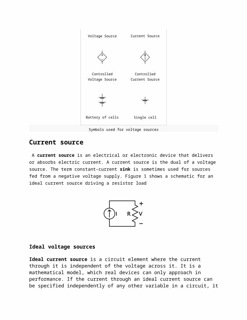
Battery of cells Single cell

Symbols used for voltage sources

Current source

A current source is an electrical or electronic device that delivers or absorbs electric current. A current source is the dual of a voltage source. The term constant-current sink is sometimes used for sources fed from a negative voltage supply. Figure 1 shows a schematic for an ideal current source driving a resistor load

Ideal voltage sources

Ideal current source is a circuit element where the current through it is independent of the voltage across it. It is a mathematical model, which real devices can only approach in performance. If the current through an ideal current source can be specified independently of any other variable in a circuit, it is called an independent current source. Conversely, if the current through an ideal current source is determined by some other voltage or current in a circuit, it is called a dependent or controlled current source. Symbols for these sources are shown in Figure 2.

An independent current source with zero current is identical to an ideal open circuit. For this reason, the internal resistance of an ideal current source is infinite. The voltage across an ideal current source is completely determined by the circuit it is connected to. When connected to a short circuit, there is zero voltage and thus zero power delivered. When connected to a load resistance, the voltage across the source approaches infinity as the load resistance approaches infinity (an open circuit). Thus, an ideal current source, if such a thing existed in reality, could supply unlimited power and so would represent an unlimited source of energy.

No real current source is ideal (no unlimited energy sources exist) and all have a finite internal resistance (none can supply unlimited voltage). However, the internal resistance of a physical current source is effectively modeled in circuit analysis by combining a non-zero resistance in parallel with an ideal current source (the Norton equivalent circuit). The connection of an ideal open circuit to an ideal non-zero current source does not represent any physically realizable system.

Independent and Dependent Sources

There are two principal types of source, namely voltage source   and current source.  Sources can be either independent or dependent upon some other quantities.

An independent voltage source  maintains a voltage (fixed or varying with time) which is not affected by any other quantity. Similarly an independent current source  maintains a current (fixed or time-varying) which is unaffected by any other quantity. The usual symbols are shown in figure 1.3.

Figure 1.3: Symbols for independent sources

Some voltage (current) sources have their voltage (current) values varying with some other variables. They are called dependent   voltage (current) sources or controlled voltage (current) sources , and their usual symbols are shown in figure 1.4.

Remarks -- It is not possible to force an independent voltage source to take up a voltage which is different from its defined value. Likewise, it is not possible to force an independent current source to take up a current which is different from its defined value. Two particular examples are short-circuiting an independent voltage source and open-circuiting an independent current source. Both are not permitted.

Figure 1.4: Symbols for dependent sources. Variables in brackets are the controlling variables whose values affect the value of the source.

Source transformation

Circuit solutions are often simplified, especially with mixed sources, by transforming a voltage into a current source, and vice versa.[1] This process is known as a source transformation, and is an application of Thevenin's theorem and Norton's theorem.

Process

Performing a source transformation is the process of using Ohms Law to take an existing voltage source in series with a resistance, and replace it with a current source in parallel with the same resistance. Remember that Ohms law states that a voltage in a material is equal to the material's resistance times the amount of current through it. Since source transformations are bilateral, one can be derived from the other. [2] Source transformations are not limited to resistive circuits however. They can be performed on a circuit involving capacitors and inductors, as long as the circuit is first put into the frequency domain. In general, the concept of source transformation is an application of Thevenin's theorem to a current source, or Norton's theorem to a voltage source.

Specifically, source transformations are used to exploit the equivalence of a real current source and a real voltage source, such as a battery. Application of Thevenin's theorem and Norton's theorem gives the quantities associated with the equivalence. Specifically, suppose we have a real current source I, which is an ideal current source in parallel with an impedance. If the ideal current source is rated at I amperes, and the parallel resistor has an impedance Z, then applying a source transformation gives an equivalent real voltage source, which is ideal, and in series with the impedance. This new voltage source V, has a value equal to the ideal current source's value times the resistance contained in the real current source . The impedance component of the real voltage source retains its real current source value.

In general, source transformations can be summarized by keeping two things in mind:

Ohm's Law Impedances remain the same

Example calculation

Figure 1. An example of a DC source transformation.

Kirchhoff's current law (KCL)

The current entering any junction is equal to the current leaving that junction. i1 + i4 = i2 + i3

This law is also called Kirchhoff's first law, Kirchhoff's point rule, Kirchhoff's junction rule (or nodal rule), and Kirchhoff's first rule.

The principle of conservation of electric charge implies that:

At any node (junction) in an electrical circuit, the sum of currents flowing into that node is equal to the sum of currents flowing out of that node.

or

The algebraic sum of currents in a network of conductors meeting at a point is zero.

Recalling that current is a signed (positive or negative) quantity reflecting direction towards or away from a node, this principle can be stated as:

n is the total number of branches with currents flowing towards or away from the node.

This formula is valid for complex currents:

The law is based on the conservation of charge whereby the charge (measured in coulombs) is the product of the current (in amperes) and the time (in seconds).

Kirchhoff's voltage law (KVL)

The sum of all the voltages around the loop is equal to zero. v1 + v2 + v3 - v4 = 0

This law is also called Kirchhoff's second law, Kirchhoff's loop (or mesh) rule, and Kirchhoff's second rule.

The principle of conservation of energy implies that

The directed sum of the electrical potential differences (voltage) around any closed circuit is zero.

or

More simply, the sum of the emfs in any closed loop is equivalent to the sum of the potential drops in that loop.

or

The algebraic sum of the products of the resistances of the conductors and the currents in them in a closed loop is equal to the total emf available in that loop.

Similarly to KCL, it can be stated as:

Here, n is the total number of voltages measured. The voltages may also be complex:

This law is based on the conservation of "energy given/taken by potential field" (not including energy taken by dissipation). Given a voltage potential, a charge which has completed a closed loop doesn't gain or lose energy as it has gone back to initial potential level.

Mesh analysis

Mesh current method is a method that is used to solve planar circuits for the voltage and currents at any place in the circuit. Planar circuits are circuits that can be drawn on a plane with no wires overlapping each other. Mesh analysis uses Kirchhoff’s voltage law to solve these planar circuits. The advantage of using mesh analysis is that it creates a systematic approach to solving planar circuits and reduces the number of equations needed to solve the circuit for all of the voltages and currents

The reason to use mesh currents instead of just using KCL and KVL to solve a problem is that the mesh currents can account for any unnecessary currents that may be drawn in when using KCL and KVL. Mesh analysis ensures that the least possible number of equations regarding currents is used, greatly simplifying the problem.

Setting up the equations

Figure 3: Simple Circuit using Mesh Analysis

If a voltage source is present within the mesh loop, the voltage at the source is either added or subtracted depending on if it is a voltage drop or a voltage rise in the direction of the mesh current. For a current source that is not contained between two meshes, the mesh current will take the positive or negative value of the current source depending on if the mesh current is in the same or opposite direction of the current source.[2] The following is the same circuit from above with the equations needed to solve for all the currents in the circuit.

Once the equations are found, the system of linear equations can be solved by using any technique to solve linear equations.

[edit] Special cases

There are two special cases in mesh current: supermesh and dependent sources.

[edit] Supermesh

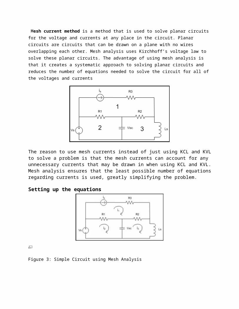
Figure 4: Circuit with a supermesh. Supermesh occurs because the current source is in between the essential meshes.

A supermesh occurs when a current source is contained between two essential meshes. To handle the supermesh, first treat the circuit as if the current source is not there. This leads to one equation that incorporates two mesh currents. Once this equation is formed, an equation is needed that relates the two mesh currents with the current source. This will be an equation where the current source is equal to one of the mesh currents minus the other. The following is a simple example of dealing with a supermesh.[1]

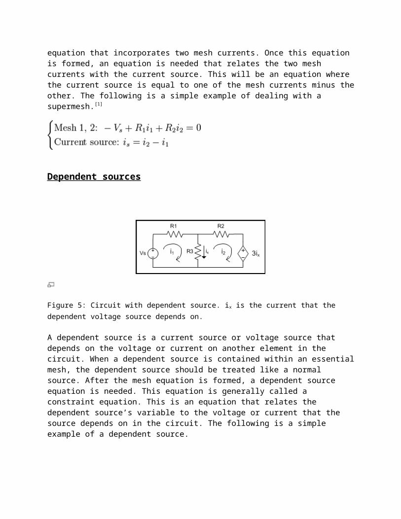
Dependent sources

Figure 5: Circuit with dependent source. ix is the current that the dependent voltage source depends on.

A dependent source is a current source or voltage source that depends on the voltage or current on another element in the circuit. When a dependent source is contained within an essential mesh, the dependent source should be treated like a normal source. After the mesh equation is formed, a dependent source equation is needed. This equation is generally called a constraint equation. This is an equation that relates the dependent source’s variable to the voltage or current that the source depends on in the circuit. The following is a simple example of a dependent source.

Nodal analysis

In electric circuits analysis, nodal analysis, node-voltage analysis, or the branch current method is a method of determining the voltage (potential difference) between "nodes" (points where elements or branches connect) in an electrical circuit in terms of the branch currents.

In analyzing a circuit using Kirchhoff's circuit laws, one can either do nodal analysis using Kirchhoff's current law (KCL) or mesh analysis using Kirchhoff's voltage law (KVL). Nodal analysis writes an equation at each electrical node, requiring that the branch currents incident at a node must sum to zero. The branch currents are written in terms of the circuit node voltages. As a consequence, each branch constitutive relation must give current as a function of voltage; an admittance representation. For instance, for a resistor, Ibranch = Vbranch * G, where G (=1/R) is the admittance (conductance) of the resistor.

Examples

Basic example circuit with one unknown voltage, V1.

The only unknown voltage in this circuit is V1. There are three connections to this node and consequently three currents to consider. The direction of the currents in calculations is chosen to be away from the node.

1. Current through resistor R1: (V1 - VS) / R1

2. Current through resistor R2: V1 / R2

3. Current through current source IS: -IS

With Kirchhoff's current law, we get:

This equation can be solved in respect to V1:

Finally, the unknown voltage can be solved by substituting numerical values for the symbols. Any unknown currents are easy to calculate after all the voltages in the circuit are known.

[edit] Supernodes

In this circuit, VA is between two unknown voltages, and is therefore a supernode.

In this circuit, we initially have two unknown voltages, V1 and V2. The voltage at V3 is already known to be VB because the other terminal of the voltage source is at ground potential.

The current going through voltage source VA cannot be directly calculated. Therefore we can not write the current equations for either V1 or V2. However, we know that the same current leaving

node V2 must enter node V1. Even though the nodes can not be individually solved, we know that the combined current of these two nodes is zero. This combining of the two nodes is called the supernode technique, and it requires one additional equation: V1 = V2 + VA.

The complete set of equations for this circuit is:

By substituting V1 to the first equation and solving in respect to V2, we get:

Thévenin's theorem

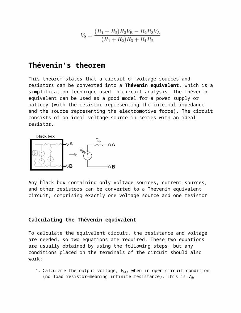
This theorem states that a circuit of voltage sources and resistors can be converted into a Thévenin equivalent, which is a simplification technique used in circuit analysis. The Thévenin equivalent can be used as a good model for a power supply or battery (with the resistor representing the internal impedance and the source representing the electromotive force). The circuit consists of an ideal voltage source in series with an ideal resistor.

Any black box containing only voltage sources, current sources, and other resistors can be converted to a Thévenin equivalent circuit, comprising exactly one voltage source and one resistor

Calculating the Thévenin equivalent

To calculate the equivalent circuit, the resistance and voltage are needed, so two equations are required. These two equations are usually obtained by using the following steps, but any conditions placed on the terminals of the circuit should also work:

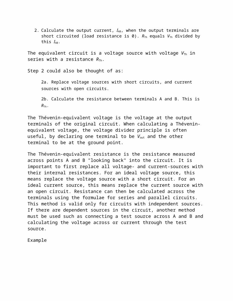
1. Calculate the output voltage, VAB, when in open circuit condition (no load resistor—meaning infinite resistance). This is VTh.

2. Calculate the output current, IAB, when the output terminals are short circuited (load resistance is 0). RTh equals VTh divided by this IAB.

The equivalent circuit is a voltage source with voltage VTh in series with a resistance RTh.

Step 2 could also be thought of as:

2a. Replace voltage sources with short circuits, and current sources with open circuits.

2b. Calculate the resistance between terminals A and B. This is RTh.

The Thévenin-equivalent voltage is the voltage at the output terminals of the original circuit. When calculating a Thévenin-equivalent voltage, the voltage divider principle is often useful, by declaring one terminal to be Vout and the other terminal to be at the ground point.

The Thévenin-equivalent resistance is the resistance measured across points A and B "looking back" into the circuit. It is important to first replace all voltage- and current-sources with their internal resistances. For an ideal voltage source, this means replace the voltage source with a short circuit. For an ideal current source, this means replace the current source with an open circuit. Resistance can then be calculated across the terminals using the formulae for series and parallel circuits. This method is valid only for circuits with independent sources. If there are dependent sources in the circuit, another method must be used such as connecting a test source across A and B and calculating the voltage across or current through the test source.

Example

Step 0: The original circuit

Step 1: Calculating the equivalent output voltage

Step 2: Calculating the equivalent resistance

Step 3: The equivalent circuit

In the example,

calculating the equivalent voltage:

(notice that R1 is not taken into consideration, as above calculations are done in an open circuit condition between A and B, therefore no current flows through this part, which means there is no current through R1 and therefore no voltage drop along this part)

Calculating equivalent resistance:

Conversion to a Norton equivalentMain article: Norton's theorem

A Norton equivalent circuit is related to the Thévenin equivalent by the following:

Norton's theorem

The Norton equivalent is used to represent any network of linear sources and impedances, at a given frequency. The circuit consists of an ideal current source in parallel with an ideal impedance (or resistor for non-reactive circuits).

Any black box containing only voltage sources, current sources, and resistors can be converted to a Norton equivalent circuit

[edit] Calculation of a Norton equivalent circuit

The Norton equivalent circuit is a current source with current INo in parallel with a resistance RNo. To find the equivalent,

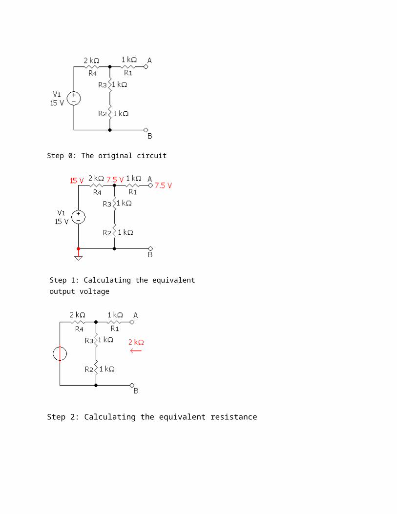
1. Find the Norton current INo. Calculate the output current, IAB, with a short circuit as the load (meaning 0 resistance between A and B). This is INo.

2. Find the Norton resistance RNo. When there are no dependent sources (i.e., all current and voltage sources are independent), there are two methods of determining the Norton impedance RNo.

Calculate the output voltage, VAB, when in open circuit condition (i.e., no load resistor — meaning infinite load resistance). RNo equals this VAB divided by INo.

or

Replace independent voltage sources with short circuits and independent current sources with open circuits. The total resistance across the output port is the Norton impedance RNo.

Example of a Norton equivalent circuit

Step 0: The original circuit

Step 1: Calculating the equivalent output current

Step 2: Calculating the equivalent resistance

Step 3: The equivalent circuit

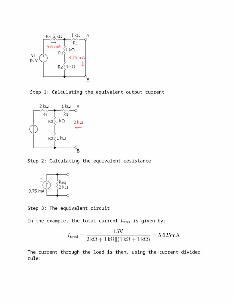
In the example, the total current Itotal is given by:

The current through the load is then, using the current divider rule:

And the equivalent resistance looking back into the circuit is:

So the equivalent circuit is a 3.75 mA current source in parallel with a 2 kΩ resistor

Conversion to a Thévenin equivalent

A Norton equivalent circuit is related to the Thévenin equivalent by the following equations:

Superposition theorem

The superposition theorem for electrical circuits states that the response (Voltage or Current) in any branch of a bilateral linear circuit having more than one independent source equals the algebraic sum of the responses caused by each independent source acting alone, while all other independent sources are replaced by their internal impedances.

To ascertain the contribution of each individual source, all of the other sources first must be "turned off" (set to zero) by:

1. Replacing all other independent voltage sources with a short circuit (thereby eliminating difference of potential. i.e. V=0, internal impedance of ideal voltage source is ZERO (short circuit)).

2. Replacing all other independent current sources with an open circuit (thereby eliminating current. i.e. I=0, internal impedance of ideal current source is infinite (open circuit).

This procedure is followed for each source in turn, then the resultant responses are added to determine the true operation of the circuit. The resultant circuit operation is the superposition of the various voltage and current sources.

The superposition theorem is very important in circuit analysis. It is used in converting any circuit into its Norton equivalent or Thevenin equivalent.

Applicable to linear networks (time varying or time invariant) consisting of independent sources, linear dependent sources, linear passive elements Resistors, Inductors, Capacitors and linear transformers.

Star to Delta Transforms

We can now solve simple series, parallel or bridge type resistive networks using Kirchoff´s

Circuit Laws, mesh current analysis or nodal voltage analysis techniques but in a balanced 3-

phase circuit we can use different mathematical techniques to simplify the analysis of the circuit

and thereby reduce the amount of math's involved which in itself is a good thing. Standard 3-

phase circuits or networks take on two major forms with names that represent the way in which

the resistances are connected, a Star connected network which has the symbol of the letter, Υ

(wye) and a Delta connected network which has the symbol of a triangle, Δ (delta). If a 3-phase,

3-wire supply or even a 3-phase load is connected in one type of configuration, it can be easily

transformed or changed it into an equivalent configuration of the other type by using either the

Star Delta Transformation or Delta Star Transformation process.

A resistive network consisting of three impedances can be connected together to form a T or "Tee" configuration but

the network can also be redrawn to form a Star or Υ type network as shown below.

T-connected and Equivalent Star Network

As we have already seen, we can redraw the T resistor network to produce an equivalent Star or

Υ type network. But we can also convert a Pi or π type resistor network into an equivalent Delta

or Δ type network as shown below.

Pi-connected and Equivalent Delta Network.

Having now defined exactly what is a Star and Delta connected network it is possible to

transform the Υ into an equivalent Δ circuit and also to convert a Δ into an equivalent Υ circuit

using a the transformation process. This process allows us to produce a mathematical

relationship between the various resistors giving us a Star Delta Transformation as well as a

Delta Star Transformation.

These transformations allow us to change the three connected resistances by their equivalents

measured between the terminals 1-2, 1-3 or 2-3 for either a star or delta connected circuit.

However, the resulting networks are only equivalent for voltages and currents external to the star

or delta networks, as internally the voltages and currents are different but each network will

consume the same amount of power and have the same power factor to each other.

Delta Star Transformation

To convert a delta network to an equivalent star network we need to derive a transformation

formula for equating the various resistors to each other between the various terminals. Consider

the circuit below.

Delta to Star Network.

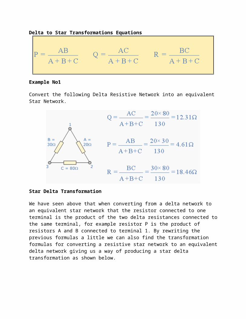
Delta to Star Transformations Equations

 

 

Example No1

Convert the following Delta Resistive Network into an equivalent Star Network.

Star Delta Transformation

We have seen above that when converting from a delta network to an equivalent star network

that the resistor connected to one terminal is the product of the two delta resistances connected to

the same terminal, for example resistor P is the product of resistors A and B connected to

terminal 1. By rewriting the previous formulas a little we can also find the transformation

formulas for converting a resistive star network to an equivalent delta network giving us a way of

producing a star delta transformation as shown below.

Star to Delta Network.

The value of the resistor on any one side of the delta, Δ network is the sum of all the two-product

combinations of resistors in the star network divide by the star resistor located "directly

opposite" the delta resistor being found. For example, resistor A is given as:

with respect to terminal 3 and resistor B is given as:

with respect to terminal 2 with resistor C given as:

with respect to terminal 1.By dividing out each equation by the value of the denominator we end

up with three separate transformation formulas that can be used to convert any Delta resistive

network into an equivalent star network as given below.

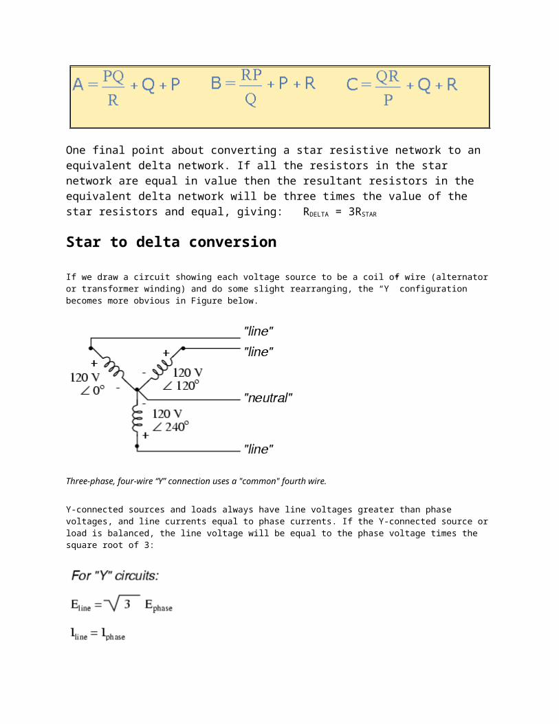
Star Delta Transformation Equations

 

 

One final point about converting a star resistive network to an equivalent delta network. If all the

resistors in the star network are equal in value then the resultant resistors in the equivalent delta

network will be three times the value of the star resistors and equal, giving:   RDELTA = 3RSTAR

Star to delta conversion

If we draw a circuit showing each voltage source to be a coil of wire (alternator or transformer winding) and do some slight rearranging, the “Y” configuration becomes more obvious in Figure below.

Three-phase, four-wire “Y” connection uses a "common" fourth wire.

Y-connected sources and loads always have line voltages greater than phase voltages, and line currents equal to phase currents. If the Y-connected source or load is balanced, the line voltage will be equal to the phase voltage times the square root of 3:

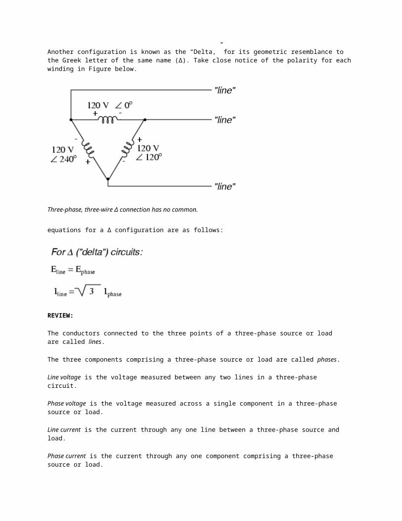
Another configuration is known as the “Delta,” for its geometric resemblance to the Greek letter of the same name (Δ). Take close notice of the polarity for each winding in Figure below.

Three-phase, three-wire Δ connection has no common.

equations for a Δ configuration are as follows:

REVIEW:

The conductors connected to the three points of a three-phase source or load are called lines.

The three components comprising a three-phase source or load are called phases.

Line voltage is the voltage measured between any two lines in a three-phase circuit.

Phase voltage is the voltage measured across a single component in a three-phase source or load.

Line current is the current through any one line between a three-phase source and load.

Phase current is the current through any one component comprising a three-phase source or load.

In balanced “Y” circuits, line voltage is equal to phase voltage times the square root of 3,

while line current is equal to phase current.

In balanced Δ circuits, line voltage is equal to phase voltage, while line current is equal to phase current times the square root of 3.

Δ-connected three-phase voltage sources give greater reliability in the event of winding failure than Y-connected sources. However, Y-connected sources can deliver the same amount of power with less line current than Δ-connected sources.

Real, reactive, and apparent powers

If the loads are purely reactive, then the voltage and current are 90 degrees out of phase. For half of each cycle, the product of voltage and current is positive, but on the other half of the cycle, the product is negative, indicating that on average, exactly as much energy flows toward the load as flows back. There is no net energy flow over one cycle. In this case, only reactive energy flows—there is no net transfer of energy to the load.

Practical loads have resistance, inductance, and capacitance, so both real and reactive power will flow to real loads. Power engineers measure apparent power as the magnitude of the vector sum of real and reactive power. Apparent power is the product of the root-mean-square of voltage and current.

The complex power is the vector sum of real and reactive power. The apparent power is the magnitude of the complex power.  Real power (P)  Reactive power (Q)  Complex power (S)  Apparent Power (|S|)  Phase of Current (φ)

Real power (P) or active power[1]: watt [W] Reactive power (Q): volt-ampere reactive [var] Complex power (S): volt-ampere [VA] Apparent Power (|S|), that is, the absolute value of complex power S: volt-ampere [VA] Phase of Current (φ), the angle of difference (in degrees) between voltage and current; Current

lagging Voltage (Quadrant I Vector), Current leading voltage (Quadrant IV Vector)

In the diagram, P is the real power, Q is the reactive power (in this case positive), S is the complex power and the length of S is the apparent power.

Reactive power does not transfer energy, so it is represented as the imaginary axis of the vector diagram. Real power moves energy, so it is the real axis.

Apparent power is conventionally expressed in volt-amperes (VA) since it is the product of rms voltage and rms current. The unit for reactive power is expressed as var, which stands for volt-amperes reactive. Since reactive power transfers no net energy to the load, it is sometimes called "wattless" power

Power factor

The ratio between real power and apparent power in a circuit is called the power factor. It's a practical measure of the efficiency of a power distribution system

The power factor is one when the voltage and current are in phase. It is zero when the current leads or lags the voltage by 90 degrees. Power factors are usually stated as "leading" or "lagging" to show the sign of the phase angle, where leading indicates a negative sign.

Purely capacitive circuits cause reactive power with the current waveform leading the voltage wave by 90 degrees, while purely inductive circuits cause reactive power with the current waveform lagging the voltage waveform by 90 degrees. The result of this is that capacitive and inductive circuit elements tend to cancel each other out.

Where the waveforms are purely sinusoidal, the power factor is the cosine of the phase angle (φ) between the current and voltage sinusoid waveforms. Equipment data sheets and nameplates often will abbreviate power factor as "cosφ" for this reason.

Example: The real power is 700 W and the phase angle between voltage and current is 45.6°. The power factor is cos(45.6°) = 0.700. The apparent power is then: 700 W / cos(45.6°) = 1000 VA.

Reactive powerthe portion of power flow that is temporarily stored in the form of electric or magnetic fields, due to inductive and capacitive network elements, and returned to source is known as the reactive power.

AC connected devices that store energy in the form of a magnetic field include inductive devices called reactors, which consist of a large coil of wire. When a voltage is initially placed across the coil a magnetic field builds up, and it takes a period of time for the current to reach full value. This causes the current to lag the voltage in phase, and hence these devices are said to absorb reactive power.

Unbalanced poly phase systems

While real power and reactive power are well defined in any system, the definition of apparent power for unbalanced polyphase systems is considered to be one of the most controversial topics in power engineering. Originally, apparent power arose merely as a figure of merit. Major delineations of the concept are attributed to Stanley's Phenomena of Retardation in the Induction

Coil (1888) and Steinmetz's Theoretical Elements of Engineering (1915). However, with the development of three phase power distribution, it became clear that the definition of apparent power and the power factor could not be applied to unbalanced poly phase systems. In 1920, a "Special Joint Committee of the AIEE and the National Electric Light Association" met to resolve the issue. They considered two definitions:

that is, the quotient of the sums of the real powers for each phase over the sum of the apparent power for each phase.

that is, the quotient of the sums of the real powers for each phase over the magnitude of the sum of the complex powers for each phase.

The 1920 committee found no consensus and the topic continued to dominate discussions. In 1930 another committee formed and once again failed to resolve the question. The transcripts of their discussions are the lengthiest and most controversial ever published by the AIEE (Emanuel, 1993). Further resolution of this debate did not come until the late 1990s.

Basic calculations using real numbers

A perfect resistor stores no energy, so current and voltage are in phase. Therefore there is no reactive power and P = S. Therefore for a perfect resistor

For a perfect capacitor or inductor there is no net power transfer, so all power is reactive. Therefore for a perfect capacitor or inductor:

Where X is the reactance of the capacitor or inductor.

If X is defined as being positive for an inductor and negative for a capacitor then we can remove the modulus signs from Q and X and get