MARCH 2003

UNIT OF ACTION KEY PERFORMANCE PARAMETER

(KPP) ANALYSIS FINAL REPORT

DEPARTMENT OF THE ARMY

UNIT OF ACTION MANEUVER BATTLE LABORATORY FORT KNOX, KENTUCKY 40121

20030812 122

REPORT DOCUMENTATION PAGE Form Approved 0MB No. 0704-0188

Public reporting burden for this collection of information is estimated to average 1 hour per response, including the time for reviewing instructions, searching existing data sources, gathering and maintaining the data needed, and completing and reviewing the collection of information. Send comments regarding this burden estimate or any other aspect of this collection of Information, Including suggestions for reducing this burden, to Washington Headquarters Services, Directorate for Information Operations and Reports, 1215 Jefferson Davis Highway, Suite 1204, Arlington, VA 22202-4302, and to the Office of Management and Budget, Paperwork Reduction Project (0704-0188), Washington, DC 20503.

1. AGENCY USE ONLY ILeave blank} 2. REPORT DATE March 2(X)3

3. REPORT TYPE AND DATES COVERED Final 27 January - March 20)3

4. TITLE AND SUBTITLE Unit of Action Key Performance Parameter (KPP) Analysis

AUTHOR(S) Mr. Lawrence G. Vowels Mr. Myron Spears

5. FUNDING NUMBERS

7. PERFORMING ORGANIZATION NAME(S) AND ADDRESS(ES) Unit of Action Maneuver Battle Laboratory Fort Knox, KY 40121

8. PERFORMING ORGANIZATION REPORT NUMBER

9. SPONSORING / MONITORING AGENCY NAME(S) AND ADDRESS(ES) 10. SPONSORING / MONITORING AGENCY REPORT NUMBER

11. SUPPLEMENTARY NOTES

12a. DISTRIBUTION / AVAILABILITY STATEMENT Approved for public release; distribution unlimited.

12b. DISTRIBUTION CODE

13. ABSTRACT (Maximum 200 words) The Unit of Action Maneuver Battle Laboratory (UAMBL) in conjimction with Computer Science Corporation and other TRADOC agencies and schools conducted an analysis on selected key performance parameters of the Future Combat System (PCS) in order to investigate threshold level of these parameters for the Operational Requirements Document (ORD). The UAMBL m conjimction with contractor and other TRADOC personnel conducted the analysis in the Maneuver Warfare Test Bed (MWTB) during the period 27 January - March 2(X)3. The objectives of the analysis was to determine the impact of situational awareness (SA) on battle outcome; to determine the situational awareness threshold necessary for mission accomplishment; to determine the impact of network dependability on battle outcome; and to determine the impact of reduced operational availability on battle outcome.

14. SUBJECT TERMS Unit of Action, Future Combat System, Key Performance Parameter, Situational Awareness, Operational Availability

17, SECURITY CLASSIFICATION OF REPORT

Unclassified

18. SECURITY CLASSIFICATION OF THIS PAGE

Unclassified

19. SECURITY CLASSIFICATION OF ABSTRACT

Unclassified

15. NUMBER OF PAGES 28

16. PRICE CODE

20. LIMITATION OF ABSTRACT

NSN 7540-01-280-5500 Standard Form 298 (Rev. 2-89) Prescribed by ANSI Std. Z39-18 298-102

USAPPCV1.00

NOTICES

DISTRIBUTION STATEMENT

Approved for public release; distribution is unlimited.

DISCLAIMER

The findings in this report are not to be construed as an official Department of the Army position, unless so designated by other authorized documents.

11

UNIT OF ACTION KPP ANALYSIS

STUDY GIST

THE REASON FOR PERFORMING THE ANALYSIS to conduct an analysis on selected key performance parameters of the Future Combat System (PCS) in order to investigate threshold levels of these parameters for the Operational Requirements Document (ORD).

THE PRINCIPAL RESULTS of this analysis are: The effect of situational awareness on battle outcome was significant. In two out of three measures examined the effect on battle outcome changed significantly when situational awareness dropped below 73% of total enemy detected. Network dependability had little effect on battle outcome. The effectiveness of the combined arms battalion drops significantly when the operational availability level drops from 95 to 92.5 percent.

SCOPE: The analysis focused on a single piece of Eastern European terrain. The terrain w^ in the Balkans and consists of the area near the Pristina airfield. The combined arms task force was battalion size. This battalion was supported by Comanche helicopters from the unit of action (UA) and a typical unit of employment (UE) slice of support weapons. The UE weapons were primarily non-line-of-sight (NLOS) platforms. A limited number of BEWSS iterations were produced for each examined case due to the limited time available for the analysis. The BEWSS simulation was unable to reproduce intermittent network failures. Consequently the network dependability was based strictly on the delay in messages getting through the network.

THE STUDY OBJECTIVES were: To determine the impact of situational awareness (SA) on battle outcome. Determine the situational awareness threshold necessary for mission accomplishment. Determine the impact of network dependability on battle outcome. Determine the impact of reduced operational availability on battle outcome.

THE BASIC APPROACH use to accomplish this evaluation was limited to examination of the operational effectiveness of the combined arms battalion within the BEWSS simulation,

THE STUDY PROPONENT/AGENCY was the Unit of Action Maneuver Battle Laboratory.

Ill

CONTENTS

SF 298 i

NOTICES ii

STUDY GIST iii

TABLE OF CONTENTS iv

LIST OF FIGURES v

ABSTRACT vi

INTRODUCTION 1

OBJECTIVES 1

SCOPE 1

METHODOLOGY 2

RUN MATRIX 2

SCENARIO 3

ANALYSIS 8

INSIGHTS AND CONCLUSIONS 22

IV

LIST OF FIGURES

Number 1 Analysis Methodology

2 Scenario (Phase 1)

3 Scenario (Phase 2)

4 Scenario (Phase 3)

5 Situational Awareness

6 LER Comparison

7 Standoff Range Comparison

8 Network Dependability Comparison

9 Standoff Range Comparison

10 Red Kills Over Time

11 Operational Availability Methodology

12 LER Comparison

13 Total Threat Kills

14 LER Comparison Engagement 2

15 Total Threat BCilled by Engagement 2

Page 2

6

7

8

9

10

10

11

12

13

14

16

18

19

21

ABSTRACT

The Unit of Action Maneuver Battle Laboratory (UAMBL) in conjunction with Computer Science Corporation and other TRADOC agencies and schools conducted an analysis on selected key performance parameters of the Future Combat System (FCS) in order to investigate threshold level of these parameters for the Operational Requirements Document (ORD). The UAMBL in conjunction with contractor and other TRADOC personnel conducted the analysis in the Maneuver Warfare Test Bed (MWTB) during the period 27 January - March 2003. The objectives of the analysis was to determine the impact of situational awareness (SA) on battle outcome; to determine the situational awareness threshold necessary for mission accomplishment; to determine the impact of network dependability on battle outcome; and to determine the impact of reduced operational availability on battle outcome.

VI

KEY PERFORMANCE PARAMETER ANALYSIS (U)

1. (U) INTRODUCTION.

a. (U) In January-March 2003, the Unit of Action Maneuver Battle Laboratory (UAMBL) in conjunction with Computer Science Corporation and other TRADOC agencies and schools conducted an analysis on selected key performance parameters of the Future Combat System (FCS) in order to investigate threshold levels of these parameters for the Operational Requirements Document (ORD).

b. (U) This report details the conduct of the BEWSS gaming that was performed at UAMBL, Fort Knox in support of this effort.

c. (U) The UAMBL, in concert with personnel from Computer Science Corporation and TRADOC Analysis Center personnel conducted the analysis in the Mounted Warfare Test Bed (MWTB) during the period 27 January - March 2003.

2. (U) OBJECTIVES.

a. (U) Determine the impact of situational awareness (SA) on battle outcome.

b. (U) Determine the situational awareness threshold necessary for mission accomplishment.

c. (U) Determine the impact of network dependability on battle outcome.

d. (U) Determine the impact of reduced operational availability on battle outcome.

3. (U) SCOPE.

a. (U) The analysis examined warfighting on a single piece of Eastern European terrain. The terrain was in the Balkans and consists of the area near the Pristina airfield.

b. (U) The combined arms task force was battalion size. This battalion was supported by Comanche helicopters from the unit of action (UA) and a typical unit of employment (UE) slice of support weapons. The UE weapons were primarily non-line- of-sight (NLOS) platforms.

c. (U) A limited number of BEWSS iterations were produced for each examined case due to the limited time available for the analysis.

d. (U) The BEWSS simulation was unable to reproduce intermittent network failures. Consequently the network dependability was based strictly on the delay in messages getting through the network.

4. (U) METHODOLOGY.

a. (U) The methodology used to accomplish this analysis using BEWSS is as follows.

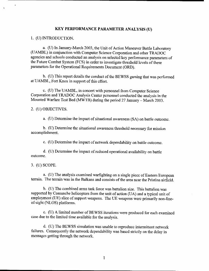
(1) (U) To examine the tenets of KPP #2 (Battle Command) which encompasses the first three objectives, the availability of Red units to detection was varied over time to create varying levels of Blue situational awareness. For these varying levels of situational awareness the network dependability was varied. This matrix of 12 runs enabled us to examine the level of situational awareness that is sufficient for mission accomplishment. These runs also allowed us to examine the network dependability. Figure 1 below portrays this methodology.

Figure 1. (U) Analysis Methodology

(2) (U) From these cases a base case was selected as necessary and sufficient to achieve success in this scenario. The last set of cases was designed to elicit understanding of KPP #5 (Sustainability). The effect of beginning operational availability on the outcome of the battle and the effects of combat damage to vehicles within the battalion were examined. The base case used 100% operational availability (AQ ). This set of cases examined the effect of entering the battle with less than 100% AQ. Specific cases examined included starting the battle at 95%) and 90%) Ao.

5. (U) RUN MATRIX. A run matrix is displayed in table 1 that shows the changes in organization and situational awareness capabilities that were made for each case.

Table 1. (U) Run Matrix

KPP Run ,^^, „'^'*7;:!'. "^"RangT"' "P'^'""*'™'" f""-"'» Level Dependability * Availability Battle

2

1 L I 90% None 100% All 2 II 90% None 100% All 3 III 90% None 100% All 4 IV 90% None 100% All 5 I 70% None 100% All 6 II 70% None 100% All 7 III 70% None 100% All 8 IV 70% None 100% All 9 I 50% None 100% All 10 II 50% None 100% All 11 III 50% None 100% All 12 IV 50% None 100% All

v^ J

Establish Base Case for Subsequent Runs

5 21 Base Base None > 95% All 22 Base Base None 95% All 23 Base Base None 92.5% All 24 Base Base None 90% All

6. (U) SCENARIO.

a. (U) General. The scenario consists ofa Blue Combined Arms Battalion (CAB) assaulting the remnants ofa Threat Mechanized Brigade after a shaping fight. The scenario takes place in Eastern Europe in an 80x80 kilometer box in the vicinity of Pristina, Yugoslavia, The weather was clear and the battle occurred during the day.

b, (U) Blue Forces. The Blue Combined Arms Battalion is augmented by systems from the UA brigade and the Unit of Employment (UE). Specifically, six 155mm cannon are fi-om the NLOS battalion and two RAH-66 helicopters from the aviation detachment are from the brigade. Three HIMARS systems and two Class IV UAV launcher/controller systems from the UE are also part of the Blue force. Table 2 displays the Blue forces that take part in this scenario.

Table 2. (U) Blue Forces

Blue Systems

Quantity Killer? Killing Systems

FCS Infantry Carrier (ICV) 24 X 24 LRP 32 X 32 Javelin 6 X 6 FCS Mounted Combat System 18 X 18 C2 Vehicle (C2V) 21 X 21 NLOS Mortar 8 X 8 FCS R&S V 9 X 9 Armed Robotic Veh (ARV) 9 0 FTTS-MS (Class III bulkA^) 2 0 FTTS-U 6 0 AVLB 9 0 ACE 2 0 FCS MED Veh 6 0 UAV CL I 5 0 UAV CL II 4 0 UAV CL III 10 0 NLOS-LS 12 X 12 GBS Radar 1 0 NLOS Cannon 6 X 6 HIMARS 3 X 3 RAH-66 4 X 4 UAV CL IV 4 0

201 143

c. (U) Threat Forces. Threat forces are a portion of a mechanized brigade that is defending a nearby airfield. The brigade has been attrited but remains quite capable of defending the territory. Table 3 shows the Threat systems that remain and are employed in the defense.

Tables. (U) Threat Forces

Red Systems

Quantity Killer? Killing Systems

1V16 12 0 2B9 5 X 5 2S19 21 X 21 2S6 19 X 19 2S9 45 X 45 BM21 3 X 3 BMP2 57 X 57 BMP3 5 X 5 BTR-80A 5 X 5 CMCB 2 0 D20 33 X 33 DRAEGA(DECOY) 9 0 FDC 10 0 GAZ 54 0 KA50 2 X 2 MRL300 3 X 3 SA-13 4 X 4 SA-17 4 X 4 AT-5 GNR 49 X 49 FO 71 X 71 RIFLEMAN 83 X 83 SCOUT 31 X 31 RUAV 2 0 SA-15 8 X 8 T-72 46 X 46 T-90S 6 X 6 RADAR GROUND 1 0

590 500

d. (U) Scenario Phases, This battle is divided into three separate phases. The first phase begins with the maneuver force beginning movement through sparse enemy to a position of advantage. The second phase is the maneuver companies occupying the position of advantage and attriting the enemy from a standoff range. While each of these two phases is taking place the indirect fires systems are shaping the area to be assaulted

and attrits the enemy indirect fire assets. The final phase is the close assault carried out by the maneuver companies.

(1) (U)ManeuverOutof Contact to a Posifion of Advantage. The first phase of the battle involved the tactical movement of the maneuver companies out of contact to a position of advantage. Preceding this movement the scouts have maneuvered forward and have secured posifions for non-line-of-sight (NLOS) systems. The unmatmed aerial vehicles are also out building situational awareness and providing targeting information to the NLOS systems. The NLOS systems are engaging enemy systems based on this information. Figure 2 displays this phase of the scenario on a map that has a 25 kilometer grid.

Figure 2. (U) Scenario (Phase 1) Maneuver Out of Contact to a Position of Advantage

(2) (U) Standoff Battle. In this second phase of the battle the maneuver close to the standoff position. The mortars with maneuver control systems and infantry carrier vehicles begin to engage the enemy from a standoff position. The NLOS systems continue to attrit the enemy from positions of advantage. This portion of the scenario is displayed in figure 3 below.

Figure 3. (U) Scenario (Phase 2) Attack from Standoff Position

(3) (U) Close Assault, The scenario is culminated in the third phase with the close assault by the maneuver companies. The maneuver control systems and infantry carrier systems continue to attack the enemy with line-of-sight (LOS) and beyond line-of-sight (BLOS) fires. The NLOS systems continue to engage the enemy formation throughout its depth. This phase is displayed in figure 4 shown below.

Figure 4. (U) Scenario (Phase 3) Close Assault

7. (U) ANALYSIS.

a. (U) Overall. The analysis performed was by design, short term. The objective was to obtain as much knowledge as possible about a number of key performance parameters (KPP) in a relatively short period of time. Everyone associated with the analysis acknowledged that the BEWSS simulation was not optimum for the investigation. It was believed that it offered the best chance of providing some insights on the KPP in the short time frame available.

b. (U) Key Performance Parameter #2. As previously stated in the methodology section, the examination of this KPP was undertaken through development of levels of situational awareness. After this development, network dependability was examined for each level of situational awareness.

(1) (U) Situational Awareness.

(a.) (U) General. The first step in the analysis was to develop differing levels of situational awareness. This was accomplished by varying the detectability of the Threat systems. The changes in detectability were made in both the optical and thermal bands. In the lower two levels of SA radar detection ranges were also altered. This permitted certain Threat systems to remain undetected for longer periods of time even though they were positioned in the open and susceptible to detection by UA assets.

The situational awareness was primarily driven by the Class III and IV unmanned aerial vehicle assets. The goal was to bound situational awareness at the levels of 50% and 80% of all Threat systems detected by the time the UA maneuver assets reached the standoff positions. Shown in figure 5 are the results of the base case situational awareness as measured in detections of Threat systems.

Levels of Situational Awareness

Percent Red Detected

Time (Seconds)

Figures. (U) Situational Awareness

As seen in this figure the situational awareness as measured in terms of Threat systems detected by the time the maneuver assets had reached the position of advantage achieved the bounding of situational awareness (SA) that was desired.

(b.) (U) Loss Exchange Ratio (LER). The first measure of effectiveness that w^ used to examine situational awareness was loss exchange ratio. Loss exchange ratio is defined as follows:

Total Red System Losses LOSS EXCHANGE RATIO = Total Blue System Losses

Investigation of endgame loss exchange ratio (LER) over the four levels of SA shows a significant drop in LER between SA levels II (73%) and III (58%). This drop is portrayed in figure 6.

Situational Awareness

LER vs. Situational Awareness Level Average of all Network Dependability Variants within SA Level

10

Average Loss g Exchange Ratio

(LER) 7

6

5 I n m IV

Situational Awareness Level

Figure 6. (U) LER Comparison

(c.) (U) The next measure of performance used to examine situational awareness was standoff range. Standoff range was defined as the difference in kill range for all UA and Threat systems. Standoff range displays a dramatic drop between SA levels I (87%) and II (73%). This reduction can be clearly seen in figure 7. The drop in standoff range is primarily attributable to the lack of beyond line-of-sight (BLOS) kills achieved by the mounted combat system (MCS).

Average Standoff Range Average Standoff Range vs. Situational Awareness

Level Ayerage of all Network Dependability Variants within SA Level

Average Standoff

Range (KM)

I II III IV

Situational Awareness Level

Figure 7. (U) Standoff Range Comparison

10

(d.) (U) Key System Losses. Other measures of performance examined in the analysis included the losses of key systems on both the Blue and Red side. On the Threat (Red) side the losses of T-72 tanks was examined. The trend was as situational awareness increased the losses in Threat T-72 tanks increased. The increase was dramatic when moving from SA level II (73%) to SA level I (87%). The increase in T-72 losses averaged nearly 7.5 vehicles due to the increased SA. Similarly the losses of Blue MCS systems increased as situational awareness decreased. The incre^ed losses were attributed to the Blue force not detecting as many Threat systems and attriting them prior to the assault phase. Thus during the assauh the MCS systems encoimtered more Threat systems and w^ forced to deal with them at close range. The range of MCS losses varied from three losses at SA level I (87%) to more than four and a half at SA level IV (51%).

(2) (U) Network Dependability.

(a.) (U) General. Network dependability was defined as the latency or loss of data via the network. Accordingly we varied network dependability by delaying information delivered by message. The values for the delay times were associated with levels of dependability varying between 50 and 90 percent. In the simulation all messages got through there was an increased latency factor as dependability moved from 90 to 50 percent. The same measures of effectiveness and performance were examined in the analysis of network dependability as with situational awareness,

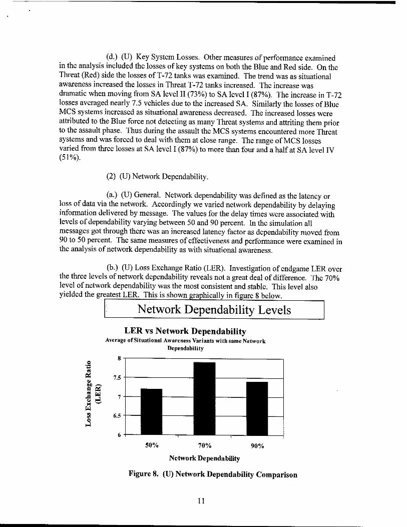
(b.) (U) Loss Exchange Ratio (LER). Investigation of endgame LER over the three levels of network dependability reveals not a great deal of difference. The 70% level of network dependability was the most consistent and stable. This level also yielded the greatest LER. This is shown graphically in figure 8 below.

Network Dependability Levels

LER vs Network Dependability Average of Situational Awareness Variants with same Network

Dependability

a -

"7 5-

<7 - ^ H

S ^ - 1 1

6 - 1 1 1

50% 70% 90%

Networii Dependability

Figure 8. (U) Network Dependability Comparison

11

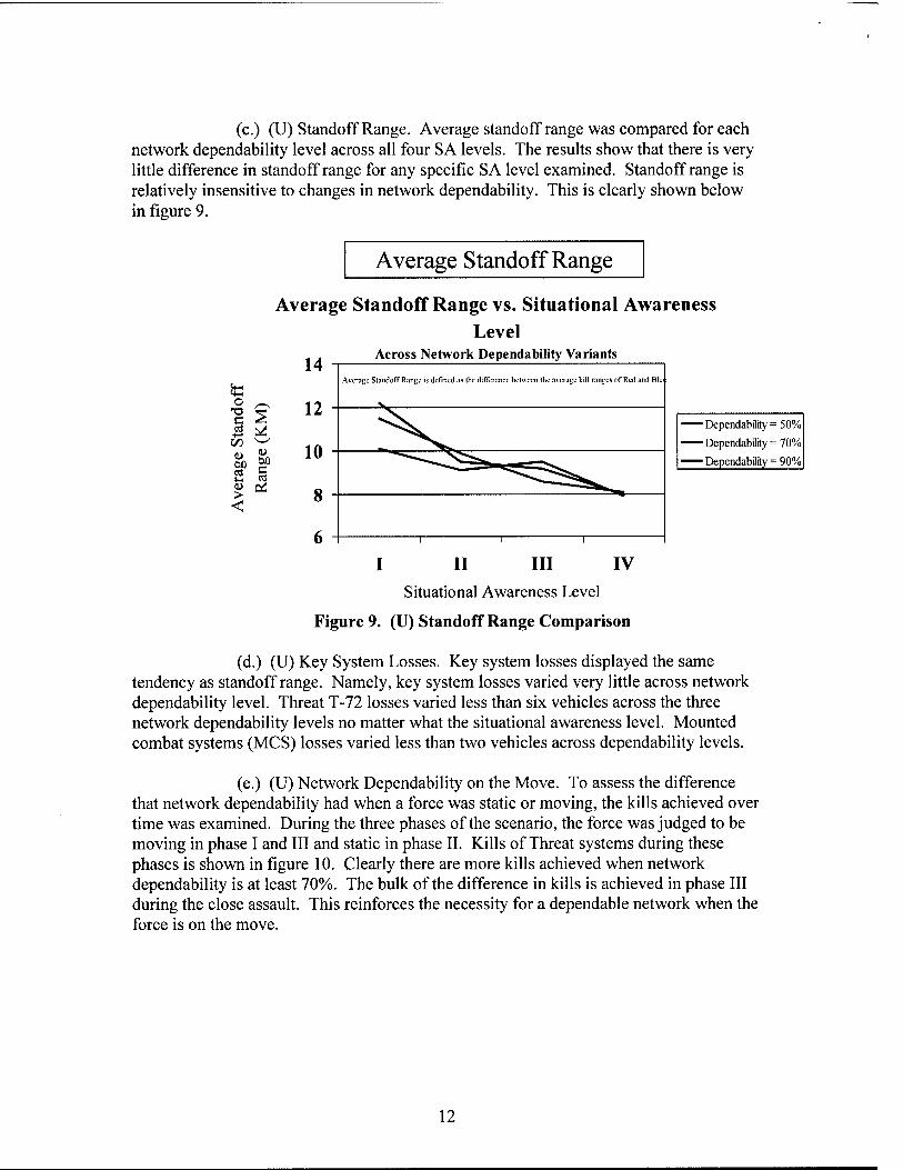
(c.) (U) Standoff Range. Average standoff range was compared for each network dependability level across all four SA levels. The results show that there is very little difference in standoff range for any specific SA level examined. Standoff range is relatively insensitive to changes in network dependability. This is clearly shown below in figure 9.

Average Standoff Range

Average Standoff Range vs. Situational Awareness Level

Across Network Dependability Variants 14

<4-( <+H o

T3 f 12 +-• ^ r/1 ^^

c 10

>J C3

> CC 8 <

A\cragc SlandofT Range is defined as the difference between the a\cragc kill ranges of Red and Blu

■Dependability =50%

■Dependability =70%

■ Dependability = 90%

I II III IV

Situational Awareness Level

Figure 9. (U) Standoff Range Comparison

(d.) (U) Key System Losses. Key system losses displayed the same tendency as standoff range. Namely, key system losses varied very little across network dependability level. Threat T-72 losses varied less than six vehicles across the three network dependability levels no matter what the situational awareness level. Mounted combat systems (MCS) losses varied less than two vehicles across dependability levels.

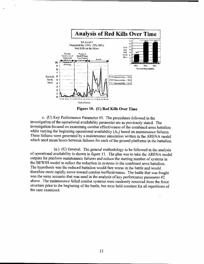
(e.) (U) Network Dependability on the Move. To assess the difference that network dependability had when a force was static or moving, the kills achieved over time was examined. During the three phases of the scenario, the force was judged to be moving in phase I and III and static in phase II. Kills of Threat systems during these phases is shown in figure 10. Clearly there are more kills achieved when network dependability is at least 70%. The bulk of the difference in kills is achieved in phase III during the close assault. This reinforces the necessity for a dependable network when the force is on the move.

12

Analysis of Red Kills Over Time SA Level I

Dependability (50%, 70%, 90%) Red Kills on the Move

50% 70% 90%

Network Dependability

- Dependability = 90%

^—Dependability = 70%

-Dependability ■= 50%

3.9 4JZ 4A 4.1 S S.3 iS 5.8 5.1 6.4 6.7 6.9 7.2 7.5 ?.g 8.1 83 8.6 S.»

Time (Hours)

Figure 10. (U) Red Kills Over Time

c. (U) Key Performance Parameter #5. The procedures followed in the investigation of the operational availability parameter are as previously stated. The investigation focused on examining combat effectiveness of the combined arms battalion while varying the beginning operational availability (Ao) based on maintenance failures. These failures were generated by a maintenance simulation written in the ARENA model which used mean hours between failures for each of the ground platforms in the battalion.

(a.) (U) General. The general methodology to be followed in the analysis of operational availability is shown in figure 11. The plan was to take the ARENA model outputs for platform maintenance failures and reduce the starting number of systems in the BEWSS model to reflect the reduction in systems in the combined arms battalion. The hypothesis was the reduced battalion would fare worse in the battle and would therefore more rapidly move toward combat ineffectiveness. The battle that was fought was the same scenario that w^ used in the analysis of key performance parameter #2 above. The maintenance failed combat systems were randomly removed from the force structure prior to the beginning of the battle, but were held constant for all repetitions of the case examined.

13

Varying Operational Availability (A^)

From a Parallel Operational Availability Analysis Effort Using ARENA:

Worst or(he i CAB'S

Operational Availability (A„) - Combat Power Impact [

UACAB ICV 25 MCS 18 C2V 20 NLOS Mori 8 RSV 9 MV 7 rrrs 37 RMV 2

ARV 21 MULE 18

NLOS Bn (sliceJ NLOS Cannon 6 1 NLOS LS J^

72 hr^ Pulse y

Vi>c\ ftiit incfudc

FCS Platform

Losses

NLOSCannnn

J"'alr- Comhnf Power

OBD Valiir

Aci > 95%

What is the impact of operational availability on battle outcome?

Assume the CAB has undergone 72 hours of continuous operations (out of enemy contact) prior to the attack

Vary the STARTEX conditions in the BEWSS/IDEAS model to reflect the Combat Power impact at three different A^ levels:

- >95%

- - 95%

- 90%

Make subsequent runs using the previous end of battle state as the STARTEX for the new battle

Determine at what point the CAB becomes combat ineffective at each A„ level

Figure 11. (U) Operational Availability Methodology

(b.) (U) ARENA Output. The output of the ARENA model that was used for input into BEWSS is displayed in table 4 below. The ARENA model was only run for three levels of operational availability. These levels were >95%, 95% and 90%. Table 4 shows entries for an operational availability level of 92.5%). These values were interpolated using the 90%) and 95%o levels. Subsequently the ARENA model was run at the 92.5%) level and the only value that was different from the values put into BEWSS was the NLOS carmon value of two maintenance losses. Based on the ARENA simulation this value should have been one maintenance loss at the 92.5%) operational availability level.

14

Table 4. (U) ARENA Model Inputs

FCS Platform

Losses Ao>95% Ao = 95% Ao = 92.5% Ao = 90%

ICV 1 3 4 5

MCS 1 2 3 4 C2V 1 2 3 4

NLOS Mort 1 1 2 2 RSV 1 1 2 2 MV 1 1 2 2

FTTS 2 4 6 8 RMV 0 1 1 1

ARV 1 1 2 2 MULE 1 2 3 4

NLOSC 1 1 Ci3i 2

NLOS LS 1 2 3 4 Total 12 21 33 40

Combat .93 .88 .81 .77

(c.) (U) First Engagement. The first portion of the analysis examines the results of the first engagement fought by the combined arms battalion.

(1.) (U) Loss Exchange Ratio (LER). The first measure examined in this portion of the analysis was loss exchange ratio. The loss exchange ratio was examined at the end of each phase of the battle. Figure 12 portrays the LER charted for each of the operational availability levels at the end of each battle phase. It is important to note that the LER at the end of phases II and III shows a decline between the Ao levels 95% and 92.5%. The approximately 30% decline in loss exchange ratio between these levels was also present between the Ao levels 95% and 90%.

15

Loss Exchange

Ratio (LER)

Snapshots of Loss Exchange Ratio (LER)

10-' _^^ 9-' 1 8-' ^ ■ _ 7-

1 « i n ■

6- 5- 4- i i -

■ After Phase I

■ After Phase II

D After Phase III

3-

2-

1-

0- r Base Case Ao>95% Ao = 95% Ao = 92.5% Ao = 90%

Figure 12. (U) LER Comparison

(2.) (U) Remaining Combat Power. The next measure used to examine Ao was battalion combat power remaining after the battle. This was measured by examining the top six killing systems with the UA combined arms battalion with the number that they entered the battle and the remaining force after the battle. A measure of failure for the battalion was preset at the loss of six MCS or six ICV. ft was felt by the leadership of UAMBL that losses of this magnitude would make the unit combat ineffective and not likely to enter into a subsequent battle until the combat power was at least partially restored. Table 5 displays the results of this measure. The blocks highlighted in red show where the battalion was judged combat ineffective after this engagement. The right column in the table shows the combat platforms remaining after the engagement. The combat losses recorded here represent the catastrophic (K) or mobility and firepower (M/F) kills. Mobility only and firepower only kills are not reflected in the combat losses column.

16

Table 5. (U) Remaining Combat Power

Remaining Combat Power

Ao S^tem Stalling Systein^

Maiiitenance Losses

Combat Losses

Total Losses

Remaining S^tems

100%

MCS 18 0 3 3 15 ICV 24 0 0.8 0.8 23.2 Mortar 8 0 0.4 0.4 7.6 C2V 21 0 3.1 3.1 17.9 NLOS Cannon 6 0 0 0 6 NLOS-LS 12 0 1.7 1.7 10.3

>95%

MCS

i

1 2 3 15 ICV 1 0.72 1.72 22.28 Mortar 1 0.2 1.2 6.8 C2V 1 3.8 4.8 16.2 MLOS Cannon 1 0 1 5 NLOS-LS 1 1.4 2.4 9.6

95%

MCS

-'

2 3.4 5.4 12.6 ICV 3 0.4 3.4 20.6 Mortar 1 0 1 7 C2V 1 3.2 4.2 16.8 HLOS Cannon 1 2 3 3 HLOS-LS 2 0 2 10

92.5%

MCS 3 2.6

^ 12.4

ICV 4 2.2 17.8 Mortar 2 0 2 6 C2V 2 2.2 4.2 16.8 HLOS Cannon 2 0 2 4 NDDS-LS 3 2.2 5.2 6.8

90%

MCS

}

4 2.4

^ 11.6

ICV 5 1.2 17,8 Mortar 2 0 2 6 C2V 2 1.6 3.6 17.4 NLOS Cannon 2 0 2 4 NLOS-LS 4 1.6 5.6 6.4

(3.) (U) Total Threat Kills, The next measure evaluated in the analysis was the total number of Threat systems killed by elements of the combined arms battalion. It was expected that the number of Threat systems killed would decrease as the Ao decreased. It was only logical that m the number of UA platforms present in the scenario declined due to maintenance failures that there would be fewer Threat systems killed. Figure 13 portrays a picture of Threat systems killed remaining relatively constant for Ao levels between 100% and 95% with a greater than 10% drop at the 92.5% level. This drop in the number of Threat systems killed w^ primarily due to the number of mounted combat system kills recorded.

17

Threat Killed by Blue

□ other

□ Mortar

■ NLOSC

■ ICV

■ HIMARS

■ NLOSLS

□ MCS

Base Case

Ao>95 Ao=95 Ao=92.5 Ao=90

Figure 13. (U) Total Threat Kills

(d.) (U) Second Engagement. A follow-on analysis was performed which examined the results of the combined arms battalion engaging the enemy again in the exact same scenario. This engagement took place with the combat losses from the first engagement added to the maintenance losses to arrive at the total reduction in starting systems for this second engagement.

(1.) (U) Loss Exchange Ratio. The first measure examined in this portion of the analysis was loss exchange ratio. The loss exchange ratio was examined at the end of each phase of the battle. Figure 14 portrays the LER charted for each of the operational availability levels at the end of each battle phase. Notice that the LER drops for each phase of the battle at the 92.5% level of operational availability.

18

Loss Exchange

Ratio (LER)

Loss Exchange Ratio (LER) After Engagement 2

■ After Phase I ■ After Phase II □ After Phase III

Base Case Ao > 95% Ao = 95% Ao = 92.5%

Figure 14. (U) LER Comparison Engagement 2

(2.) (U) Remaining Combat Power. The next measure examined in the analysis w^ the remaining combat power of the battahon. Table 6 below displays the remaining combat power of the battalion after the second engagement. Notice that the battalion at none of the Ao levels is able to survive the second engagement without losing six MCS. Only the 100% level was able to complete the second engagement without losing six ICV.

19

Table 6. (U) Remaining Combat Power Engagement 2

Remaining Combat Power Engagement 2

Ac

Starting Systems

Maintenance Losses

Combat Losses

Mobility Firepower

Losses

Cumm Losses

(w/MFL)

Cumm Losses

(w/o MFL)

100%

15 1.8 1.8 8.3 4.8 23.2 0.4 0 1.4 1.2 7.6 0 1.2 0.4 17.9 2 5.8 5.1

6 0 0.5 0 103 1.4 4.2 3.1

>95%

15 2.8 1 8 5.8 22.28 0.8 0 2.52 2.52

6.8 0 2 1.2 16.2 0.4 6 5.2

5 0 1.2 1 9.6 2 5.6 4.4

95%

12.6 1.4 0.6 8.8 5S

6.8 5.8 20.6 2.4 0

7 0 1.8 1 16.8 1.4 6 5.6

5 0 1.2 1 8 1.4 5.8 5.4

92.5%

12.4 2.5 1 10.9 7.95

8.1 7.95 17.8 1.75 0

6 0 2.4 2 16.8 2.25 6.85 6.45

4 0 2 2 6.8 1.5 7.9 6.7

90%

11.6 17.8

6 17.4

4 6.4

(3.) (U) Total Threat Kills. The next measure examined in the analysis is the total Threat systems killed by the combined arms battalion. Figure 15 displays the results from this examination. It should be noted that it is similar to the results from the first engagement. The total number of kills drops off at the 92.5% level AQ. Nearly all of the difference in Threat kills can be accounted for in the examination of kills achieved by the MCS.

20

180

Total Threat Killed by Blue Engagement 2

Base Case Ao>95 Ao=95

B Other D Mortar ■ NLOS C ■ ICV ■ HIMARS ■ NLOS LS OMCS

Ao=92.5

Figure 15. (U) Total Threat Killed by Blue Engagement 2

d. (U) Conclusions.

(1.) (U) Key Performance Parameter 2, The conclusions drawn about this performance parameter are as follows. The combined arms battalion combat performance drops significantly between situational awareness levels between 73 and 57 percent. The average kill range decreases as situational awareness levels drop. There is a significant drop in average kill range when the situational awareness level moves from 87 to 73 percent. Red tank (T72) losses decrease as situational awareness decreases. Red tank losses suffer a significant decrease when situational awareness goes from 87 to 73 percent. Unit of action MCS losses increase as situational awareness decreases. Network dependability shows no trend when examined using loss exchange ratio. Standoff range was also insensitive to changes in network dependability. Key system losses also did not react to changes in network dependability. The key finding under network dependability was a large change in kills on the move when network dependability was lowered below 70%.

(2.) (U) Key Performance Parameter 5, The conclusions drawn about this performance parameter are as follows. The effectiveness of the combined arms battaHon drops significantly when the operational availability level drops from 95 to 92.5 percent. The remaining combat power of the combined arms battalion w^ at an unacceptable after the battalion engagement when the operational availability was at the 92.5 and 90 percent levels. The total Threat systems killed by the battalion suffered significantly

21

when the operational availability level decreased from 95 to 92.5 percent. The kills achieved by the battalion MCS had the most effect on this decrease in Threat systems killed. These same conclusions could also be drawn when a second engagement was fought without replacing any of the maintenance failed or combat damaged systems from the first engagement.

8. (U) INSIGHTS AND CONCLUSIONS. The primary insights and conclusions to be drawn from this analysis are as follows. The effect of situational awareness on battle outcome was significant. In two out of three measures examined the effect on battle outcome changed significantly when situational awareness dropped below 73% of total enemy detected. Network dependability had little effect on battle outcome. The effectiveness of the combined arms battalion drops significantly when the operational availability level drops from 95 to 92.5 percent.

22