unit root time series econometrics 7777 - wordpress.com...augmented dickey-fuller (adf)unit root...
TRANSCRIPT

11/5/2013
1
5 November 2013Vijayamohan: CDS M Phil: Time Series 7 1
Time Series EconometricsTime Series EconometricsTime Series EconometricsTime Series Econometrics
7777
VijayamohananVijayamohananVijayamohananVijayamohanan PillaiPillaiPillaiPillai NNNN
5 November 2013Vijayamohan: CDS M Phil: Time Series 7 2
Unit Root Unit Root Unit Root Unit Root
TestsTestsTestsTests
5 November 2013Vijayamohan: CDS M Phil: Time Series 7 3
Unit Root Unit Root Unit Root Unit Root
TestsTestsTestsTests
‘Jack and Jill went up the hill, to look at the stars.“Do you see any unit roots there?”
Jack asks Jill who was using a telescope.“The stars all seem to be cointegrated”, replies Jill.’
G.S. Maddala (1998) ‘Recent Developments in Dynamic
Econometric Modelling: A Personal Viewpoint’,
Political Analysis; 7: 59-875 November 2013Vijayamohan: CDS MPhil: Time Series 5 4
Non-stationarity due to
(1)Integrated process: random walk:
Yt = Yt-1 + εt
Difference stationary process
Stochastic trend
(2) Trend: Trend stationary process
Both stochastic and deterministic trend
Non-stationarity
5 November 2013Vijayamohan: CDS MPhil: Time Series 5 5
Consequences of Non-stationarity
(1) With stationary series, possible to model the process via a fixed-coefficients equationestimated from past data.
Not possible if the structural relationship changes over time (if non-stationary).
(2) For non-stationary series, Var and Covs are functions of time:
so the conventional asymptotic theory cannotbe applied to these series.
5 November 2013Vijayamohan: CDS MPhil: Time Series 5 6
Consequences of Non-stationarity
(2) For non-stationary series, Var and Covs are functions of time: so the conventional asymptotic theory cannot be applied to these series.
For example: In a regression of Yt on Xt:
If Xt is non-stationary, Var(Xt) ↑↑↑↑ infinitely, and dominates the Cov(Yt, Xt):
Then the OLS estimator does not have an asymptotic distribution.
====ββββ̂ )(),( ttt XVarXYCov

11/5/2013
2
5 November 2013Vijayamohan: CDS MPhil: Time Series 5 7
Consider two unrelated RW processes:
Yt = Yt–1 + Ut; Ut ∼∼∼∼ IIN(0, σσσσU2)
Xt = Xt–1 + Vt; Vt ∼∼∼∼ IIN(0, σσσσV2);
Cov(Ut ,Vt) = 0.
Consequence of unit root (non-stationarity):
5 November 2013Vijayamohan: CDS MPhil: Time Series 5 8
Consequence of unit root (non-stationarity):
0 50 100 150 200 250 300
-10
-5
0
5
10
15
20y x
0 50 100 150 200 250 300
-10
-5
0
5
10
15
20y x
Yt = Yt–1 + Ut; Ut ∼∼∼∼ IIN(0, σσσσU2)
Xt = Xt–1 + Vt; Vt ∼∼∼∼ IIN(0, σσσσV2);
Cov(Ut ,Vt) = 0.
5 November 2013Vijayamohan: CDS MPhil: Time Series 5 9
Consequence of unit root (non-stationarity):
0 50 100 150 200 250 300
-3
-2
-1
0
1
2
3 eps ep
0 50 100 150 200 250 300
-3
-2
-1
0
1
2
3 eps ep
Ut ∼∼∼∼ IIN(0, σσσσU2)
Vt ∼∼∼∼ IIN(0, σσσσV2)
5 November 2013Vijayamohan: CDS MPhil: Time Series 5 10
Consequence of unit root (non-stationarity):
0 5 10
-0.75
-0.50
-0.25
0.00
0.25
0.50
0.75
1.00CCF-eps x ep CCF-ep x eps
0 5 10
-0.75
-0.50
-0.25
0.00
0.25
0.50
0.75
1.00CCF-eps x ep CCF-ep x eps
Cov(Ut , Vt) = 0.
Cross Correlation function
5 November 2013Vijayamohan: CDS MPhil: Time Series 5 11
Consequence of unit root (non-stationarity):
Now consider the regression:
Yt =ββββ 0 + ββββ 1 Xt + εεεεt.
We expect R2 from this regression would tend
to zero; BUT….
5 November 2013Vijayamohan: CDS MPhil: Time Series 5 12
Consequence of unit root (non-stationarity):

11/5/2013
3
5 November 2013Vijayamohan: CDS MPhil: Time Series 5 13
Consequence of unit root (non-stationarity):
5 November 2013Vijayamohan: CDS MPhil: Time Series 5 14
Granger and Newbold (1974):
High R2 and highly significant t,
but a low DW statistic.
When the regression was run
in first differences……
?
Consequence of unit root (non-stationarity):
5 November 2013Vijayamohan: CDS MPhil: Time Series 5 15
Consequence of unit root (non-stationarity):
5 November 2013Vijayamohan: CDS MPhil: Time Series 5 16
When the regression was run
in first differences,
R2 close to zero; DW close to 2: ⇒⇒⇒⇒
No relationship between Yt and Xt ; and
the high R2 obtained was ‘spurious’.
R2 > DW ⇒⇒⇒⇒ ‘Spurious Regression’.
Consequence of unit root (non-stationarity):
5 November 2013Vijayamohan: CDS MPhil: Time Series 5 17
So, check for stationarity of time series:
Classical: Autocorrelation function (ACF):
Correlogram
Fast-decreasing ACF ⇒⇒⇒⇒ Stationarity
Modern: Unit root tests:
(Augmented) Dickey-Fuller test;
Phillips-Perron non-parametric test; etc.
5 November 2013Vijayamohan: CDS MPhil: Time Series 5 18
If non-stationary series,
run regression in (first) differences as in
Classical (ARIMA) modelling
or check for Cointegration among the series
11/5/2013
4
5 November 2013Vijayamohan: CDS M Phil: Time Series 7 19
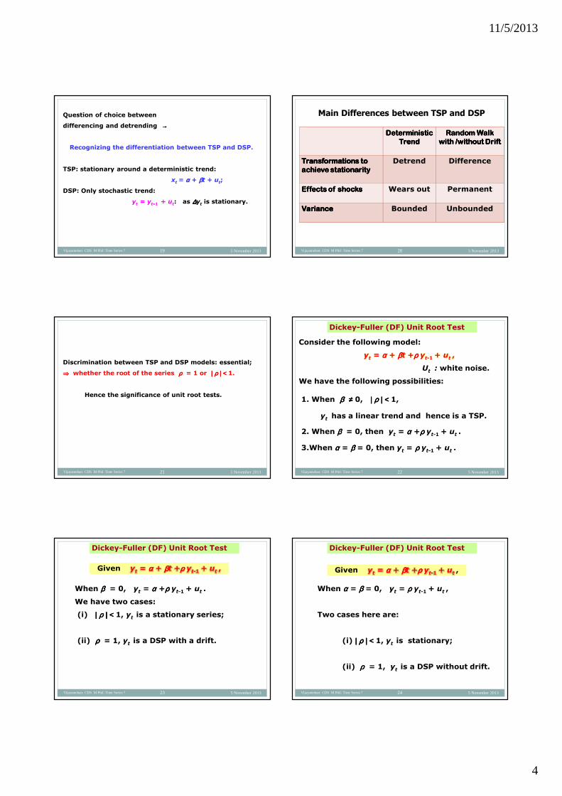
Question of choice between
differencing and detrending →→→→
Recognizing the differentiation between TSP and DSP.
TSP: stationary around a deterministic trend:
xt = αααα + ββββt + ut;
DSP: Only stochastic trend:
yt = yt−−−−1 + ut: as ∆∆∆∆yt is stationary.
5 November 2013Vijayamohan: CDS M Phil: Time Series 7 20
Deterministic Deterministic Deterministic Deterministic
Trend Trend Trend Trend
Random Walk Random Walk Random Walk Random Walk
with /without Driftwith /without Driftwith /without Driftwith /without Drift
Transformations to Transformations to Transformations to Transformations to
achieve achieve achieve achieve stationaritystationaritystationaritystationarity
Detrend Difference
Effects of shocksEffects of shocksEffects of shocksEffects of shocks Wears out Permanent
VarianceVarianceVarianceVariance Bounded Unbounded
Main Differences between TSP and DSP
5 November 2013Vijayamohan: CDS M Phil: Time Series 7 21
Discrimination between TSP and DSP models: essential;
⇒⇒⇒⇒ whether the root of the series ρρρρ = 1 or |||| ρρρρ |||| <<<< 1.
Hence the significance of unit root tests.
5 November 2013Vijayamohan: CDS M Phil: Time Series 7 22
Consider the following model:
yt = αααα + ββββt +ρρρρ yt-1+ ut ,
Ut : white noise.
We have the following possibilities:
1. When ββββ ≠≠≠≠ 0, |||| ρρρρ |||| <<<< 1,
yt has a linear trend and hence is a TSP.
2. When ββββ = 0, then yt = αααα +ρρρρ yt-1+ ut .
3.When αααα = ββββ = 0, then yt = ρρρρ yt-1+ ut .
Dickey-Fuller (DF) Unit Root Test
5 November 2013Vijayamohan: CDS M Phil: Time Series 7 23
When ββββ = 0, yt = αααα +ρρρρ yt-1+ ut .
We have two cases:
(i) |||| ρρρρ |||| <<<< 1, yt is a stationary series;
(ii) ρρρρ = 1, yt is a DSP with a drift.
Given yt = αααα + ββββt +ρρρρ yt-1+ ut ,
Dickey-Fuller (DF) Unit Root Test
5 November 2013Vijayamohan: CDS M Phil: Time Series 7 24
When αααα = ββββ = 0, yt = ρρρρ yt-1+ ut ,
Two cases here are:
(i) |||| ρρρρ |||| <<<< 1, yt is stationary;
(ii) ρρρρ = 1, yt is a DSP without drift.
Given yt = αααα + ββββt +ρρρρ yt-1+ ut ,
Dickey-Fuller (DF) Unit Root Test

11/5/2013
5
5 November 2013Vijayamohan: CDS M Phil: Time Series 7 25
Rewrite (1) yt = αααα + ββββt +ρρρρ yt-1+ ut as
∆∆∆∆ yt = αααα + ββββt +γγγγ yt-1+ ut ,
where γγγγ = (ρρρρ −−−−1).
Now, testing the null hypothesis
Ho: γγγγ = 0,
in the usual way is equivalent to testing
Ho: ρρρρ = 1.
Dickey-Fuller (DF) Unit Root Test
5 November 2013Vijayamohan: CDS M Phil: Time Series 7 26
||ly rewrite (2) yt = αααα +ρρρρ yt-1+ ut
as ∆∆∆∆ yt = αααα +γγγγ yt-1+ ut .
and (3) yt = ρρρρ yt-1+ ut ,
as ∆∆∆∆ yt = γγγγ yt-1+ ut .
Then test for Ho: γγγγ = 0,
vs. the one-sided alternative |||| ρρρρ |||| <<<< 1 .
Dickey-Fuller (DF) Unit Root Test
5 November 2013Vijayamohan: CDS M Phil: Time Series 7 27
Dickey-Fuller (DF) Unit Root Test: 3 DF Type Formulations
Note: In (1), ∆∆∆∆ yt = αααα + ββββt +γγγγ yt-1+ ut ,
where γγγγ = (ρρρρ −−−−1),
the model has both a constant and a trend;
Note: In (2), ∆∆∆∆ yt = αααα +γγγγ yt-1+ ut ,
the model has a constant; and
Note: In (3), ∆∆∆∆ yt = γγγγ yt-1+ ut ,
the model is without constant.
In a DF test all 3 formulations are considered.
5 November 2013Vijayamohan: CDS M Phil: Time Series 7 28
Dickey-Fuller (DF) Unit Root Test
But we cannot use the usual t-test to test
Ho: ρρρρ = 1,
because under the null, yt is I(1),
and hence the t-statistic does not have an asymptotic normal distribution (Dickey and Fuller 1979).
Its asymptotic distribution,
based on Wiener processes, is called
Dickey-Fuller distribution, and the statistic, Dickey-Fuller ττττ (tau) statistic.
5 November 2013Vijayamohan: CDS M Phil: Time Series 7 29
Norbert Wiener Norbert Wiener Norbert Wiener Norbert Wiener (1894 (1894 (1894 (1894 ––––1964,) 1964,) 1964,) 1964,)
American mathematician;American mathematician;American mathematician;American mathematician;
originator of cyberneticsoriginator of cyberneticsoriginator of cyberneticsoriginator of cybernetics: : : :
interdisciplinary study of the structure of interdisciplinary study of the structure of interdisciplinary study of the structure of interdisciplinary study of the structure of
regulatory systemsregulatory systemsregulatory systemsregulatory systems
Wiener process: a continuous-time stochastic processAlso called Brownian Motion
5 November 2013Vijayamohan: CDS M Phil: Time Series 7 30
Robert Brown (1773 – 1858) Scottish botanist
Brownian motion: 1827

11/5/2013
6
5 November 2013Vijayamohan: CDS M Phil: Time Series 7 31
Robert Brown (1773 – 1858) Scottish botanist
Graphs of Graphs of Graphs of Graphs of five five five five sampled sampled sampled sampled
Brownian motionsBrownian motionsBrownian motionsBrownian motions::::
5 November 2013Vijayamohan: CDS M Phil: Time Series 7 32
Critical values tabulated by Dickey and Fuller(1979) and MacKinnon (1990) for a wider range of sample.
Most of the statistic outcomes are negative;
Note: Ho: γγγγ = (ρρρρ −−−−1) = 0.
If the estimated ττττ–value is more negative
(i.e., less) than the critical value
at the chosen significance level, reject Ho.
Dickey-Fuller (DF) Unit Root Test
5 November 2013Vijayamohan: CDS M Phil: Time Series 7 33
Augmented Dickey-Fuller (ADF) Unit Root Test
In deriving the asymptotic distributions,Dickey and Fuller (1979, 1981) assumed:
ut ∼∼∼∼ iid(0,σσσσ2 ).
But, if the errors are non-orthogonal
(i.e., serially correlated),
the limiting distributions cease to beappropriate.
5 November 2013Vijayamohan: CDS M Phil: Time Series 7 34
Dickey and Fuller (1979) and
Said and Dickey (1984)
modified the DF test
by means of AR correction:
Adding lags to ‘whiten’ the residuals
gives ADF test.
Augmented Dickey-Fuller test (ADF)
Augmented Dickey-Fuller (ADF) Unit Root Test
5 November 2013Vijayamohan: CDS M Phil: Time Series 7 35
Augmented Dickey-Fuller test (ADF):
by estimating an autoregression of ∆∆∆∆yt on itsown lags and yt-1 using OLS:
When γγγγ = 0, ρρρρ = 1.
The (t -) test statistic follows the sameDF distribution (ττττ–statistic)
∑∑∑∑====
−−−−−−−− ++++∆∆∆∆++++====∆∆∆∆p
1ititi1tt .uyyy ββββγγγγ
Augmented Dickey-Fuller (ADF) Unit Root Test
5 November 2013Vijayamohan: CDS M Phil: Time Series 7 36
Test for a unit root in Yt ;
If the unit root null is not rejected
(if Yt appears I(1)),
test for a second unit root (see if Yt is I(2)):
Testing: (1):
Estimate the regression of ∆∆∆∆2Yt on a constant,
∆∆∆∆Yt–1, and the lagged values of ∆∆∆∆2Yt, and
compare the ‘t-ratio’ of the coefficient of ∆∆∆∆Yt–1
with the DF critical values.
Double Unit Roots TestingDouble Unit Roots TestingDouble Unit Roots TestingDouble Unit Roots Testing

11/5/2013
7
5 November 2013Vijayamohan: CDS M Phil: Time Series 7 37
Double Unit Roots TestingDouble Unit Roots TestingDouble Unit Roots TestingDouble Unit Roots Testing
Testing: (2):
Estimate the regression of ∆∆∆∆2Yt on Yt–1, ∆∆∆∆Yt–1,
and the lagged values of ∆∆∆∆2Yt, and
compute the usual F-statistic for testing the
joint significance of Yt–1 and ∆∆∆∆Yt–1,
using the critical values given as
ΦΦΦΦ1(2) by Hasza and Fuller (1979).
5 November 2013Vijayamohan: CDS M Phil: Time Series 7 38
Consumption
∆∆∆∆Consumption
Testing for Unit Root:(Augmented) Dickey - Fuller test:
5 November 2013Vijayamohan: CDS M Phil: Time Series 7 39
EQ( 1) Modelling ∆∆∆∆Ct by OLS (using Data.in7)The estimation sample is: 1953 (2) to 1992 (3)
Coefficient Std.Error t-value t-prob Constant 9.09221 11.46 0.793 0.429 Ct-1 -0.0106221 0.01308 -0.812 0.418
sigma 2.21251 RSS 763.648214R^2 0.00420671 F(1,156) = 0.659 [0.418]log-likelihood -348.658 DW 1.6no. of observations 158 no. of parameters 2
∆∆∆∆Ct = 9.092 – 0.0106 Ct – 1t = (0.793) (–0.812)
Critical values used in ADF test: 5%= -2.88, 1%= -3.473
Testing for Unit Root:(Augmented) Dickey - Fuller test:
5 November 2013Vijayamohan: CDS M Phil: Time Series 7 40
EQ( 1) Modelling ∆∆∆∆2Ct by OLS (using Data.in7)The estimation sample is: 1953 (3) to 1992 (3)
Coefficient Std.Error t-value t-prob Constant -0.148864 0.1736 -0.857 0.393
∆∆∆∆Ct -1 -0.813544 0.07824 -10.4 0.000
sigma 2.16501 RSS 726.524426R^2 0.410943 F(1,155) = 108.1 [0.000]**log-likelihood -343.037 DW 2.04no. of observations 157 no. of parameters 2
∆∆∆∆2Ct = –0.149 – 0.814 ∆∆∆∆Ct – 1
t = (–0.857) (–10.399)
Critical values used in ADF test: 5%=-2.88, 1%=-3.473
Testing for Unit Root:(Augmented) Dickey - Fuller test:
5 November 2013Vijayamohan: CDS M Phil: Time Series 7 41
Testing for Unit Root:(Augmented) Dickey - Fuller test:
Variable Ct in level
CONS: ADF tests (T=152, Constant; 5% = -2.88 1% = -3.47)
D-lag t-adf beta Y_1 sigma t-DY_lag t-prob AI C F-prob
5 -1.094 0.98551 2.123 -2.767 0.0064 1.551
4 -1.464 0.98038 2.171 1.253 0.2123 1.589 0.0064
3 -1.298 0.98274 2.176 1.448 0.1496 1.587 0.0110
2 -1.120 0.98516 2.184 1.687 0.0937 1.588 0.0112
1 -0.9317 0.98766 2.197 2.481 0.0142 1.594 0.0075
0 -0.6361 0.99149 2.234 1.621 0.0013
5 November 2013Vijayamohan: CDS M Phil: Time Series 7 42
Testing for Unit Root:(Augmented) Dickey - Fuller test:Variable Ct in First Difference
DCONS: ADF tests (T=152, Constant; 5% = -2.88 1% = -3.47)
D-lag t-adf beta Y_1 sigma t-DY_lag t-prob AIC F-prob
5 -4.870** 0.28208 2.132 0.06925 0.9449 1.559
4 -5.305** 0.28618 2.125 2.948 0.0037 1.546 0.9449
3 -4.448** 0.42488 2.180 -1.053 0.2941 1.591 0.0151
2 -5.313** 0.37033 2.181 -1.293 0.1981 1.585 0.0232
1 -6.801** 0.29538 2.185 -1.570 0.1185 1.583 0.0246
0 -10.08** 0.19164 2.196 1.586 0.0182

11/5/2013
8
5 November 2013Vijayamohan: CDS M Phil: Time Series 7 43
Unit Root Test for TSP vs. DSP:
Nelson and Plosser (1982)
The first ever attempt: Nelson and Plosser(1982), using the (augmented) Dickey-Fuller unit root tests:
H0: a time series belongs to DSP class against Ha: it belongs to TSP class.
Nelson and Plosser found that 13 out of 14 US macroeconomic time series that they analyzed belonged to the DSP class (the exception being the unemployment rate).
5 November 2013 Vijayamohan: CDS M Phil: Time Series 7 44
Results of Nelson and Plosser (1982, Table 5, p. 151): Critical value at 5% level: −−−−3.45
Series Sample size (T)
Lag (k) ττττ-value
Real GDP 62 2 −−−−2.99Nominal GDP 62 2 −−−−2.32Real per capita GNP 62 2 −−−−3.04Industrial production 111 6 −−−−2.53Employment 81 3 −−−−2.66Unemployment rate 81 4 −−−−3.55*GNP deflator 82 2 −−−−2.52Consumer prices 111 4 −−−−1.97Wages 71 3 −−−−2.09Real wages 71 2 −−−−3.04Money stock 82 2 −−−−3.08Velocity 102 1 −−−−1.66Interest rate 71 3 0.686
Common stock prices 100 3 −−−−2.05
5 November 2013Vijayamohan: CDS M Phil: Time Series 7 45
Other Unit Root Tests
Mushrooming of Unit root tests ever since N and P (1982) feat:
1. Sargan and Bhargava (1983): based on DW statistic;
2. Phillips and Perron (1988): non-parametric test;
3. Cochrane (1988): Variance ratio test;
4. Sims (1988): Bayesian approach to unit root testing;
5. Perron (1989): unit root test under structural break;
6. Pantula and Hall (1991): IV test in ARMA models;
7. Schmidt and Phillips (1992): LM test;
5 November 2013Vijayamohan: CDS M Phil: Time Series 7 46
8. Choi (1992): Pseudo-IV estimator test;9. Yap and Reinsel (1995): Likelihood ratio test in
ARMA models;
10. Leybourne (1995): based on forward and reverse DF regressions;
11. Park and Fuller (1995): Weighted symmetric estimator test;
12. Elliott, Rothenberg and Stock (1996): Dickey-Fuller GLS test;
Other Unit Root Tests
5 November 2013Vijayamohan: CDS M Phil: Time Series 7 47
Tests with stationarity as null:
1. Park (1990)’s J-test;
2. Kwiatkowski, Phillips, Schmidt and Shin (1992): (KPSS) test;
3. Bierens and Guo (1993): based on Cauchy distribution;
4. Leybourne and McCabe (1994): Modified KPSS test;
5. Choi (1994): based on testing for a MA unit root;
6. Arellano and Pantula (1995): based on testing for a MA unit root.
Other Unit Root Tests
5 November 2013Vijayamohan: CDS M Phil: Time Series 7 48
Panel data unit root tests:
• Levin and Lin (1993);
• Breitung and Meyer (1994)
• Quah (1994);
• Pesaran and Shin (1996);
Other Unit Root Tests

11/5/2013
9
5 November 2013Vijayamohan: CDS M Phil: Time Series 7 49
Empirical Studies by Model Unit Root
(withpossible
breaks)
Stationary
(withpossible
breaks)
Nelson and Plosser
(1982)
ADF test with no
break
13 1
Perron (1989)** Exogenous with
one break
3 11
Zivot and Andrews
(1992)*
Endogenous with
one break
10 3
Lumsdaine and
Papell (1997)*
Endogenous with
two breaks
8 5
Lee and Strazicich
(2003)**
Endogenous with
two breaks
10 4
* Assume no break(s) under the H0 of unit root.** Assume break(s) under both the null and the HA
Unit Root Tests with the Nelson and
Plosser’sData (1982) Set
5 November 2013Vijayamohan: CDS M Phil: Time Series 7 50
Time series in STATA
Tsset : Declare data to be time-series dataCopy-paste data in data editorGenerate a time variable by typing the command:
For monthly data starting with 1995 July:
. generate time = m(1995m7) + _n -1
. format t %tm
You can now tsset your data set. tsset time
time variable: time, 1995m7 to 2004m6delta: 1 month
5 November 2013Vijayamohan: CDS M Phil: Time Series 7 51
If the first observation is for the first quarter of 1990,
generate time = q(1990q1) + _n-1format time %tqtsset time
For yearly data starting at 1942 type:generate time = y(1942) + _n-1format time %tytsset time
For half yearly data starting at 1921h2 type:generate time = h(1921h2) + _n-1format time %thtsset time
5 November 2013Vijayamohan: CDS M Phil: Time Series 7 52
For weekly data starting at 1994w1 type:
. generate time = w(1994w1) + _n-1
. format time %tw
. tsset time
For daily data starting at 1jan1999 type:
. generate time = d(1jan1999) + _n-1
. format time %td
. tsset time
5 November 2013Vijayamohan: CDS M Phil: Time Series 7 53
. dfuller cons, lags(5)
Augmented Dickey-Fuller test for unit root Number of obs = 153
---------- Interpolated Dickey-Fuller ---------Test 1% Critical 5% Critical 10% Critical
Statistic Value Value Value------------------------------------------------------------------------------Z(t) -1.117 -3.492 -2.886 -2.576------------------------------------------------------------------------------MacKinnon approximate p-value for Z(t) = 0.7081
Unit Root Tests in STATA:Statistics →→→→
Time series →→→→Tests
5 November 2013Vijayamohan: CDS M Phil: Time Series 7 54
. dfuller D.cons, lags(5)
Augmented Dickey-Fuller test for unit root Number of obs = 152
---------- Interpolated Dickey-Fuller ---------Test 1% Critical 5% Critical 10% Critical
Statistic Value Value Value------------------------------------------------------------------------------Z(t) -4.870 -3.493 -2.887 -2.577------------------------------------------------------------------------------MacKinnon approximate p-value for Z(t) = 0.0000
11/5/2013
10
5 November 2013Vijayamohan: CDS M Phil: Time Series 7 55
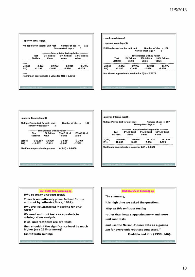
. pperron cons, lags(5)
Phillips-Perron test for unit root Number of obs = 158Newey-West lags = 5
---------- Interpolated Dickey-Fuller ---------Test 1% Critical 5% Critical 10% Critical
Statistic Value Value Value------------------------------------------------------------------------------Z(rho) -3.253 -19.993 -13.816 -11.077Z(t) -1.194 -3.491 -2.886 -2.576------------------------------------------------------------------------------MacKinnon approximate p-value for Z(t) = 0.6760
5 November 2013Vijayamohan: CDS M Phil: Time Series 7 56
. gen lcons=ln(cons)
. pperron lcons, lags(5)
Phillips-Perron test for unit root Number of obs = 158Newey-West lags = 5
---------- Interpolated Dickey-Fuller ---------Test 1% Critical 5% Critical 10% Critical
Statistic Value Value Value------------------------------------------------------------------------------Z(rho) -3.242 -19.993 -13.816 -11.077Z(t) -1.190 -3.491 -2.886 -2.576------------------------------------------------------------------------------MacKinnon approximate p-value for Z(t) = 0.6778
5 November 2013Vijayamohan: CDS M Phil: Time Series 7 57
. pperron D.cons, lags(5)
Phillips-Perron test for unit root Number of obs = 157Newey-West lags = 5
---------- Interpolated Dickey-Fuller ---------Test 1% Critical 5% Critical 10% CriticalStatistic Value Value Value
Z(rho) -146.107 -19.990 -13.814 -11.076Z(t) -10.662 -3.491 -2.886 -2.576
MacKinnon approximate p-value for Z(t) = 0.0000
5 November 2013Vijayamohan: CDS M Phil: Time Series 7 58
. pperron D.lcons, lags(5)
Phillips-Perron test for unit root Number of obs = 157Newey-West lags = 5
---------- Interpolated Dickey-Fuller ---------Test 1% Critical 5% Critical 10% Critical
Statistic Value Value Value------------------------------------------------------------------------------Z(rho) -146.064 -19.990 -13.814 -11.076Z(t) -10.656 -3.491 -2.886 -2.576------------------------------------------------------------------------------MacKinnon approximate p-value for Z(t) = 0.0000
5 November 2013Vijayamohan: CDS M Phil: Time Series 7 59
Unit Roots Test: Summing upUnit Roots Test: Summing upUnit Roots Test: Summing upUnit Roots Test: Summing up
Why so many unit root tests?
There is no uniformly powerful test for the unit root hypothesis (Stock, 1994).
Why are we interested in testing for unit roots?
We need unit root tests as a prelude to cointegration analysis.
If so, unit root tests are pre-tests;
then shouldn’t the significance level be much higher (say 25% or more)?
Isn't it Data-mining?
5 November 2013Vijayamohan: CDS M Phil: Time Series 7 60
Unit Roots Test: Summing upUnit Roots Test: Summing upUnit Roots Test: Summing upUnit Roots Test: Summing up
“In summary,
it is high time we asked the question:
Why all this unit root testing
rather than keep suggesting more and more
unit root tests
and use the Nelson-Plosser data as a guinea
pig for every unit root test suggested.”
Maddala and Kim (1998: 146).

11/5/2013
11
05 November 2013Vijayamohan: CDS MPhil: Time Series 8 61 05 November 2013Vijayamohan: CDS MPhil: Time Series 8 62
Regression of Integrated Variables
Yt
Deterministic Stochastic
Xt
Deterministic Regression valid
Spurious regression
Stochastic Spurious regression
Spurious regression
unless Xt and Yt are
cointegrated
05 November 2013Vijayamohan: CDS MPhil: Time Series 8 63
Spurious (Nonsense) regression with
integrated variables
→ using differenced variables in regression.
BUT…..
Solving non-stationarity problem via
differencing =
“Throwing the baby out with the bath water”
∵∵∵∵ differencing →→→→
“valuable long-run information being lost’’.
Cointegration
05 November 2013Vijayamohan: CDS MPhil: Time Series 8 64
∵∵∵∵ differencing →→→→ ‘valuable long-run information
being lost’’.
Regression in differences (∆∆∆∆Yt on ∆∆∆∆Xt):
short run only;
In the long run (in equilibrium): ∆∆∆∆Yt = 0 and ∆∆∆∆Xt = 0.
Most economic relationships are stated in
theory as long run relationships between
variables in their levels, not in their
differences.
Cointegration
5 November 2013Vijayamohan CDS Time Series: Introduction 65
Two seemingly irreconcilable objectives :
1. Avoid spurious regression of I(d) variables
and
2. Conserve the long-term relationship.
Hence Cointegration
(Granger 1981; Engle and Granger 1987).
05 November 2013Vijayamohan: CDS MPhil: Time Series 8 66
If two series yt and xt are both I(1),
then in general, any linear combination
of them will also be I(1);
e.g. Yt – Ct = St: All show upward trend.
Cointegration
Income
Consumption
Saving
11/5/2013
12
05 November 2013Vijayamohan: CDS MPhil: Time Series 8 67
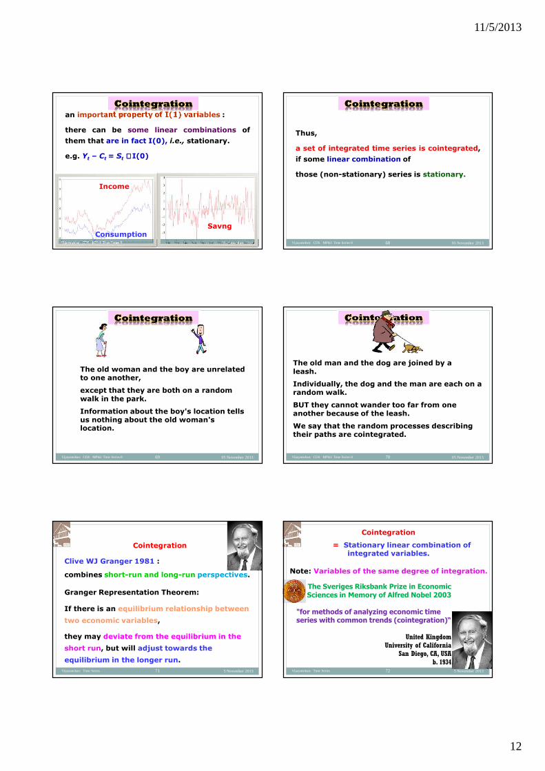
an important property of I(1) variables :
there can be some linear combinations of
them that are in fact I(0), i.e., stationary.
e.g. Yt – Ct = St ∼∼∼∼ I(0)
Cointegration
Consumption
Income
Savng
05 November 2013Vijayamohan: CDS MPhil: Time Series 8 68
Thus,
a set of integrated time series is cointegrated,
if some linear combination of
those (non-stationary) series is stationary.
Cointegration
05 November 2013Vijayamohan: CDS MPhil: Time Series 8 69
The old woman and the boy are unrelated to one another,
except that they are both on a random walk in the park.
Information about the boy's location tells us nothing about the old woman's location.
Cointegration
05 November 2013Vijayamohan: CDS MPhil: Time Series 8 70
The old man and the dog are joined by a leash.
Individually, the dog and the man are each on a random walk.
BUT they cannot wander too far from one another because of the leash.
We say that the random processes describing their paths are cointegrated.
Cointegration
5 November 2013Vijayamohan: Time Series 71
Cointegration
Clive WJ Granger 1981 :
combines short-run and long-run perspectives.
Granger Representation Theorem:
If there is an equilibrium relationship between
two economic variables,
they may deviate from the equilibrium in the
short run, but will adjust towards the
equilibrium in the longer run.
5 November 2013Vijayamohan: Time Series 72
Cointegration
= Stationary linear combination of integrated variables.
Note: Variables of the same degree of integration.
The Sveriges Riksbank Prize in Economic Sciences in Memory of Alfred Nobel 2003
"for methods of analyzing economic time series with common trends (cointegration)“
United KingdomUniversity of California San Diego, CA, USA
b. 1934

11/5/2013
13
05 November 2013Vijayamohan: CDS MPhil: Time Series 8 73
If there exists a relationship between two non
stationary I(1) series, Yt and Xt , such that the
residuals of the regression:
Yt = βXt + ut , that is, ut = Yt – βXt
are stationary, i.e., I(0), then the variables,
Yt and Xt , are said to be cointegrated.
The system is in long-run equilibrium when
E(Yt – βXt) = 0.
∴∴∴∴ ut = equilibrium error (deviation from long-
run equilibrium).
Cointegration
05 November 2013Vijayamohan: CDS MPhil: Time Series 8 74
The system is in long-run equilibrium when
E(Yt – βXt) = 0.
∴∴∴∴ ut = equilibrium error (deviation from long-
run equilibrium).
For the equilibrium to be meaningful,
equilibrium error process must be stationary.
β is called the constant of cointegration, and
the equation is called cointegrating regression
or Cointegrating vector (CV).
Cointegration
05 November 2013Vijayamohan: CDS MPhil: Time Series 8 75
Equilibrium Errors: (i.e. ut = Yt - βXt)
ut
0 timeError rarely drifts from zero
No tendency to return to zero
05 November 2013Vijayamohan: CDS MPhil: Time Series 8 76
Two series Yt and Xt are said to be cointegrated if:
1. Both are I(d), d ≠≠≠≠ 0 and the same for both series (having the same ‘wave length’); and
2. There is a linear combination of them that is I(0),
i.e., there exists ut = Yt – βXt that is I(0).
In this light, the regression of these two
variables, yt = ββββ xt + ut makes sense
(is not spurious).
Cointegration
05 November 2013Vijayamohan: CDS MPhil: Time Series 8 77
How can we distinguish between a genuine long-run relationship and a spurious regression? We need a test.
Two categories:
1. Single equation method: Residual-based test:
using (A)DF -statistic:Engle and Granger (1987): (A)EG test;
1. System (Multiple equation) method: Johansen and Juselius (1990): JJ test.
Cointegration
05 November 2013Vijayamohan: CDS MPhil: Time Series 8 78
Testing for Cointegration: Residual based tests
(1) After estimating the model, save residuals fro m static regression. Consider whether residuals are stationary.
0 90
10 20 30 40 50 60 70 80 100
-0.5
0.0
0.5
1.0
0 1 2 3 4 5 6 7 8 9 10 11 12
-0.5
0.0
0.5
1.0
residuals
ACF

11/5/2013
14
05 November 2013Vijayamohan: CDS MPhil: Time Series 8 79
We proceed in three steps :Step 1: Test that both variables have the same order
of integration , say, that they are both I(1). This can be
performed with the unit-root tests described before .
Step 2: Estimate a `long-run relationship by OLS:
yt =αααα + ββββ xt + ut
Step 3: Extract the residuals of this regression (ut )
and test for a unit-root in this series, using (A)DF test
statistic: ut has a unit root ⇒⇒⇒⇒ NO cointegration .
Testing for Cointegration: Residual based tests
(2): Cointegrating Regression (A)DF test: (Augmented) Engle-Granger test
05 November 2013Vijayamohan: CDS MPhil: Time Series 8 80
(A)EG test is a test of no-cointegration :
H0: No Cointegration (= unit root in ut)
Acceptance of a unit root in the residuals suggests that the residual term is non-stationary , which implies NO cointegration:
= Not rejecting H 0. That is,
If the estimated (A)DF ττττ–value is more negative(i.e., less) than the critical value at the chosen
significance level, reject Ho
= There IS cointegration.
Testing for Cointegration: Residual based tests:(Augmented) Engle-Granger test
05 November 2013Vijayamohan: CDS MPhil: Time Series 8 81
Testing for Cointegration: Residual based tests:(Augmented) Engle-Granger test
Step 1: Test for the order of integration of Xt and Yt:
Unit-root tests (using Data1)The sample is 4 - 300
X: ADF tests (T=297, Constant; 5% = -2.87; 1% = -3.45)D-lag t-adf beta Y_1 sigma t-DY_lag t-prob AIC F-prob2 1.941 1.0006 0.9939 -0.1358 0.8920 0.0010961 1.942 1.0006 0.9922 0.5127 0.6085 -0.005575 0.89200 2.028 1.0007 0.9910 -0.01142 0.8692
Y: ADF tests (T=297, Constant; 5%=-2.87 1%=-3.45)D-lag t-adf beta Y_1 sigma t-DY_lag t-prob AIC F-prob2 -0.9251 0.99935 0.9635 1.163 0.2459 -0.060911 -0.9554 0.99932 0.9641 -0.9526 0.3416 -0.06304 0.24590 -0.9305 0.99934 0.9640 -0.06669 0.3244
05 November 2013Vijayamohan: CDS MPhil: Time Series 8 82
Step 1: Test for the order of integration of Xt and Yt:
Testing for Cointegration: Residual based tests:(Augmented) Engle-Granger test
Unit-root tests (using Data1)The sample is 5 - 300
DX: ADF tests (T=296, Constant; 5% = -2.87; 1% = -3.45)D-lag t-adf beta Y_1 sigma t-DY_lag t-prob AIC F-prob2 -9.604** 0.057433 1.002 -0.1413 0.8878 0.017131 -11.77** 0.049579 1.000 -0.08180 0.9349 0.01045 0.88780 -16.39** 0.045016 0.9985 0.003713 0.9868
DY: ADF tests (T=296, Constant; 5% = -2.87; 1% = -3.45)D-lag t-adf beta Y_1 sigma t-DY_lag t-prob AIC F-prob2 -8.860** 0.099869 0.9527 -1.232 0.2191 -0.083491 -11.60** 0.028890 0.9535 -1.094 0.2749 -0.08507 0.21910 -18.02** -0.037637 0.9539 -0.08775 0.2589
05 November 2013Vijayamohan: CDS MPhil: Time Series 8 83
EQ( 1) Modelling Y by OLS (using Data1)The estimation sample is: 1 to 300
Coefficient Std.Error t-value t-prob Part.R^2Constant 4.85755 0.1375 35.3 0.000 0.9279X 1.00792 0.005081 198. 0.000 0.9975
sigma 0.564679 RSS 30.9296673R^2 0.997541 F(1,97) = 3.935e+004 [0.000]**log-likelihood -82.8864 DW 2.28no. of observations 99 no. of parameters 2
And save residuals.
Testing for Cointegration: Residual based tests:(Augmented) Engle-Granger test
Step 2: Estimate cointegrating regression
Yt = β0 + β1Xt + ut
05 November 2013Vijayamohan: CDS MPhil: Time Series 8 84
EQ( 6) Modelling Dresiduals by OLS (using Data1.in7)
The estimation sample is: 4 to 300
Coefficient Std.Error t-value t-prob Part.R^2residuals_1 -1.16140 0.1024 -11.3 0.000 0.5805
sigma 0.545133 RSS 27.6367834log-likelihood -75.8453 DW 1.95
Which means ∆ut = -1.161 ut-1 + et(-11.3)
CRDF test statistic = -11.3 << -3.39 = 1% Critical Value from MacKinnon.
Hence we reject null of no cointegration between X and Y.
Testing for Cointegration: Residual based tests:(Augmented) Engle-Granger test
Step 3: Check for unit root in the residuals:

11/5/2013
15
05 November 2013Vijayamohan: CDS MPhil: Time Series 8 85
Unit-root tests (using Data1)
The sample is 4 - 300
Residuals: ADF tests (T=297, Constant; 5% = -2.87; 1% = -3.39)
D-lag t-adf beta Y_1 sigma t-DY_lag t-prob AIC F-prob
2 -9.867** 0.016854 0.9869 0.4090 0.6828 -0.01308
1 -10.72** 0.040004 0.9855 -0.2931 0.7696 -0.01924 0.6828
0 -11.33** 1.16140 0.5451 -0.02568 0.8812
Testing for Cointegration: Residual based tests:(Augmented) Engle-Granger test
Step 3: Check for unit root in the residuals:
05 November 2013Vijayamohan: CDS MPhil: Time Series 8 86
Testing for Cointegration: Residual based tests:(Augmented) Engle-Granger test
Step 3: Check for stationarity (unit root) of the residuals:
0 50 100 150 200 250 300
-2.5
0.0
2.5
0 5 10
0
1
0 5 10
0
1
Residuals
ACF
PACF
05 November 2013Vijayamohan: CDS MPhil: Time Series 8 87
Testing for Cointegration: System method:Johansen – Juselius test
Most popular system method: JJ -test (Johansen1988; Johansen and Juselius 1990),
Provides two likelihood ratio (LR) tests.
(1)The trace test: tests the hypothesis that thereare at most r cointegrating vectors, and
(2) The maximum eigenvalue test: tests the nullhypothesis that there are r cointegratingvectors against the hypothesis that there arer+1 cointegrating vectors.
Johansen and Juselius (1990) recommend thesecond test as better.
05 November 2013Vijayamohan: CDS MPhil: Time Series 8 88
Testing for Cointegration: System method:Johansen – Juselius test
JJ-test is in the framework of VAR (Sims 1980)
In a VAR, all the variables are endogenous:
With two variables in a model, X and Y: two endogenous variables in VAR;
That is, two equations:
(1): Yt = a + b Xt; and (2): Xt = c + d Yt;
Thus two possible cointegrating vectors(CVs):
We need to identify the CVs.
05 November 2013Vijayamohan: CDS MPhil: Time Series 8 89
Trace test:
This tests the null hypothesis that there are at
most r (i.e., 0 ≤≤≤≤ r ≤≤≤≤ n) cointegrating vectors
(CVs)
Ho: r CVs against H1: >>>> r CVs.
Thus the first row tests Ho: r = 0 against
H1: r >>>> 0; if this is significant, Ho is rejected and
the next row is considered.
Thus the rank (r = number of CVs) is chosen as
the last significant statistic, or as zero if the first
is not significant.
Testing for Cointegration: System method:Johansen – Juselius test
05 November 2013Vijayamohan: CDS MPhil: Time Series 8 90
Testing for Cointegration: System method:Johansen – Juselius test
Maximum eigenvalue test:
This tests Ho: r CVs against H1: r + 1 CVs. Thus
the first row tests Ho: r = 0 against H1: r = 1; if
this is significant, Ho is rejected and the next
row is considered.
A potential problem with the size of these test statistics in small samples: that is, the JJprocedure tends to over-reject the null when it is true (Reimers 1992). Hence a small-sample correction is applied to these statistics, replacing T by T−−−− np, where T is the number of observations, n is the number of variables and pis the lag length of the VAR.
11/5/2013
16
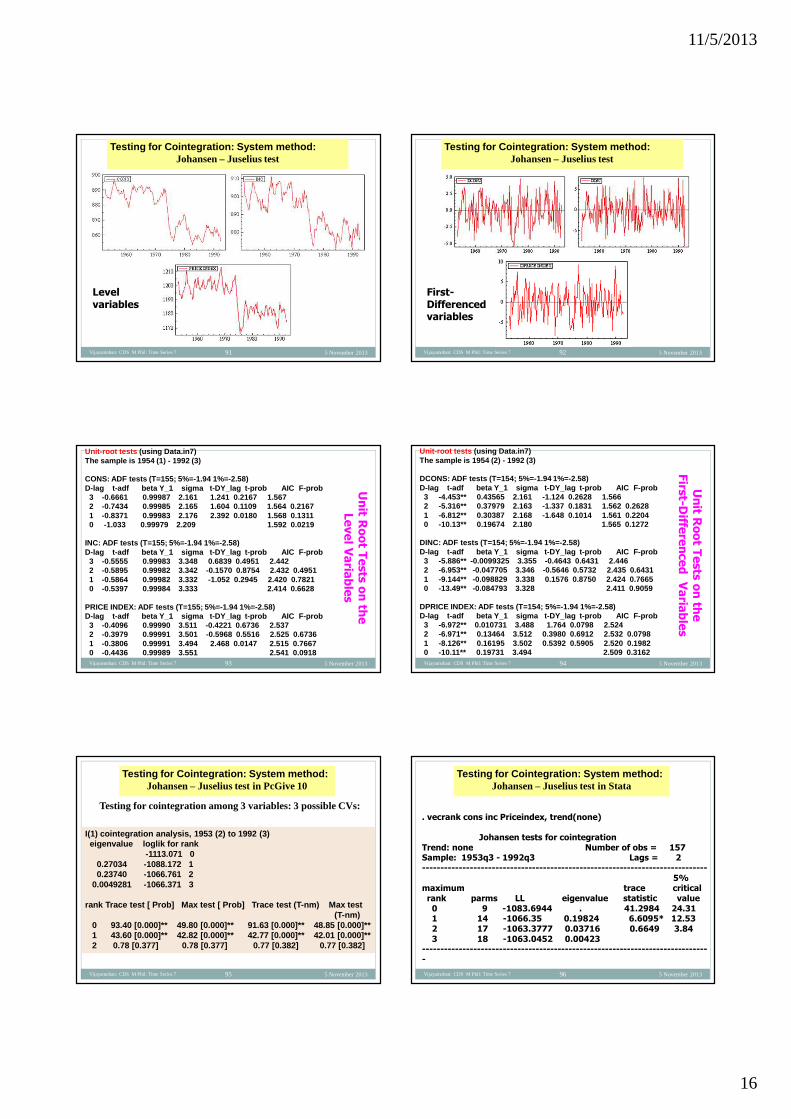
5 November 2013Vijayamohan: CDS M Phil: Time Series 7 91
Testing for Cointegration: System method:Johansen – Juselius test
Level variables
5 November 2013Vijayamohan: CDS M Phil: Time Series 7 92
Testing for Cointegration: System method:Johansen – Juselius test
First-Differenced variables
5 November 2013Vijayamohan: CDS M Phil: Time Series 7 93
Unit-root tests (using Data.in7)The sample is 1954 (1) - 1992 (3)
CONS: ADF tests (T=155; 5%=-1.94 1%=-2.58)D-lag t-adf beta Y_1 sigma t-DY_lag t-prob AIC F-prob
3 -0.6661 0.99987 2.161 1.241 0.2167 1.5672 -0.7434 0.99985 2.165 1.604 0.1109 1.564 0.21671 -0.8371 0.99983 2.176 2.392 0.0180 1.568 0.13110 -1.033 0.99979 2.209 1.592 0.0219
INC: ADF tests (T=155; 5%=-1.94 1%=-2.58)D-lag t-adf beta Y_1 sigma t-DY_lag t-prob AIC F-prob
3 -0.5555 0.99983 3.348 0.6839 0.4951 2.4422 -0.5895 0.99982 3.342 -0.1570 0.8754 2.432 0.49511 -0.5864 0.99982 3.332 -1.052 0.2945 2.420 0.78210 -0.5397 0.99984 3.333 2.414 0.6628
PRICE INDEX: ADF tests (T=155; 5%=-1.94 1%=-2.58)D-lag t-adf beta Y_1 sigma t-DY_lag t-prob AIC F-prob
3 -0.4096 0.99990 3.511 -0.4221 0.6736 2.5372 -0.3979 0.99991 3.501 -0.5968 0.5516 2.525 0.67361 -0.3806 0.99991 3.494 2.468 0.0147 2.515 0.76670 -0.4436 0.99989 3.551 2.541 0.0918
Unit R
oot Tests on th
e
Level Variables
5 November 2013Vijayamohan: CDS M Phil: Time Series 7 94
Unit-root tests (using Data.in7)The sample is 1954 (2) - 1992 (3)
DCONS: ADF tests (T=154; 5%=-1.94 1%=-2.58)D-lag t-adf beta Y_1 sigma t-DY_lag t-prob AIC F-prob
3 -4.453** 0.43565 2.161 -1.124 0.2628 1.5662 -5.316** 0.37979 2.163 -1.337 0.1831 1.562 0.26281 -6.812** 0.30387 2.168 -1.648 0.1014 1.561 0.22040 -10.13** 0.19674 2.180 1.565 0.1272
DINC: ADF tests (T=154; 5%=-1.94 1%=-2.58)D-lag t-adf beta Y_1 sigma t-DY_lag t-prob AIC F-prob
3 -5.886** -0.0099325 3.355 -0.4643 0.6431 2.4462 -6.953** -0.047705 3.346 -0.5646 0.5732 2.435 0.64311 -9.144** -0.098829 3.338 0.1576 0.8750 2.424 0.76650 -13.49** -0.084793 3.328 2.411 0.9059
DPRICE INDEX: ADF tests (T=154; 5%=-1.94 1%=-2.58)D-lag t-adf beta Y_1 sigma t-DY_lag t-prob AIC F-prob
3 -6.972** 0.010731 3.488 1.764 0.0798 2.5242 -6.971** 0.13464 3.512 0.3980 0.6912 2.532 0.07981 -8.126** 0.16195 3.502 0.5392 0.5905 2.520 0.19820 -10.11** 0.19731 3.494 2.509 0.3162
Unit R
oot Tests on th
e
First-D
ifferenced Variables
5 November 2013Vijayamohan: CDS M Phil: Time Series 7 95
Testing for Cointegration: System method:Johansen – Juselius test in PcGive 10
Testing for cointegration among 3 variables: 3 possible CVs:
I(1) cointegration analysis, 1953 (2) to 1992 (3)eigenvalue loglik for rank
-1113.071 00.27034 -1088.172 10.23740 -1066.761 2
0.0049281 -1066.371 3
rank Trace test [ Prob] Max test [ Prob] Trace test (T-nm) Max test (T-nm)
0 93.40 [0.000]** 49.80 [0.000]** 91.6 3 [0.000]** 48.85 [0.000]**1 43.60 [0.000]** 42.82 [0.000]** 42.7 7 [0.000]** 42.01 [0.000]**2 0.78 [0.377] 0.78 [0.377] 0. 77 [0.382] 0.77 [0.382]
5 November 2013Vijayamohan: CDS M Phil: Time Series 7 96
Testing for Cointegration: System method:Johansen – Juselius test in Stata
. vecrank cons inc Priceindex, trend(none)
Johansen tests for cointegrationTrend: none Number of obs = 157Sample: 1953q3 - 1992q3 Lags = 2------------------------------------------------------------------------------
5%maximum trace criticalrank parms LL eigenvalue statistic value0 9 -1083.6944 . 41.2984 24.311 14 -1066.35 0.19824 6.6095* 12.532 17 -1063.3777 0.03716 0.6649 3.843 18 -1063.0452 0.00423
-------------------------------------------------------------------------------

11/5/2013
17
5 November 2013Vijayamohan: CDS M Phil: Time Series 7 97
Testing for Cointegration: System method:Johansen – Juselius test in Stata
(input all the variables in the column for dependent variables)
In Stata
Statistics →→→→ Multivariate Time Series →→→→ Cointegrating rank of a VECM
05 November 2013Vijayamohan: CDS MPhil: Time Series 8 98
Summing Up: ‘Much Ado about Nothing’?
If ut = Yt – βXt is I(0),
yt and xt are cointegrated
(Both I(d), d ≠≠≠≠ 0 )
and the regression yt = ββββ xt + ut
is not spurious.
05 November 2013Vijayamohan: CDS MPhil: Time Series 8 99
Summing Up: ‘Full of Sound and Fury; Signifying Nothing’?
ut ~~~~ I(0) ⇒⇒⇒⇒ ut is white noise
⇒⇒⇒⇒ OLS assumptions satisfied!
So just see if OLS assumptions are satisfied!
No need for the pre-tests
(of unit root and cointegration)!
(See my book ‘Econometrics of Electricity Demand:
Questioning the Tradition’ 2010, Lambert Academic
Publishing, Germany)
5 November 2013Vijayamohan CDS Time Series: Introduction 100
Most macroeconomic variables : non stationary.
Non-stationarity problem:Consequence: Spurious Regression
Approaches: Classical Modern
Diagnosis: ACF tests Unit root tests
Solution: Differencing Differencing/Cointegration
Estimation: ARIMA (Box-Jenkins)/ VAR (Sims 1980)/MARIMA (V)ECM (Sargan 1964;(Harvey 1997) Davidson et al. 1978)/
GETS (Hendry 1987)
5 November 2013 Vijayamohan: CDS M Phil: Time Series 7
101